Testing the structure of the covariance matrix with

fewer observations than the dimensionI

Muni S. Srivastava, N. Reid

Department of Statistics100 St. George St.

Toronto Canada M5S 3G3

Abstract

We consider two hypothesis testing problems with N independent observa-tions on a single m-vector, when m > N , and the N observations on therandom m-vector are independently and identically distributed as multivari-ate normal with mean vector µ and covariance matrix Σ, both unknown. Inthe first problem, the m-vector is partitioned into two subvectors of dimen-sions m1 and m2, respectively, and we propose two tests for the independenceof the two sub-vectors that are valid as (m,N)→∞. The asymptotic distri-bution of the test statistics under the hypothesis of independence is shown tobe standard normal, and the power examined by simulations. The proposedtests perform better than the likelihood ratio test, although the latter canonly be used when m is smaller than N . The second problem addressed isthat of testing the hypothesis that the covariance matrix Σ is of the intraclasscorrelation structure. A statistic for testing this is proposed, and assessedvia simulations; again the proposed test statistic compares favorably withthe likelihood ratio test.

Keywords: attained significance level, false discovery rate, highdimensional data, independence of sub-vectors, intraclass correlation,multivariate normal distribution, p > n2000 MSC: 62H15, 62P10

IThis research was supported by the Natural Sciences and Engineering Research Coun-cil of Canada. We wish to thank Jingchunzi Shi and Xin Wang for computational assis-tance.

Email address: srivasta,reid@utstat.toronto.edu (Muni S. Srivastava, N. Reid)

Preprint submitted to Multivariate Analysis October 25, 2011

1. Introduction

Recent advances in technology to obtain DNA microarrays have madeit possible to measure quantitatively the expressions of thousands of genes.These expression levels within subjects may, however, be expected to becorrelated. Since the number of subjects, N , is usually quite small comparedto the number of genes, m, multivariate theory for the situation when m >>N needs to be developed: classical asymptotic theory requires m fixed sothat m/N → 0. Alternatively, some authors such as Dudoit et al. (2002)have suggested ordering the m genes by, for example, their sample meansand selecting a very small number of them, much smaller than N , so thatthe usual asymptotic theory can be applied. The implicit assumption is thatthe remaining genes have mean zero and thus should not have much effecton the analysis. But unless the selected set is distributed independently ofthe remaining set of variables for which the mean is zero, this remaining setcan provide significant information about the mean vector of the selected set;see, Srivastava and Khatri (1979, p. 115–118).

For example, consider the problem of classifying an individual with m-dimensional observed vector x, into two known groups with mean vectors µ,µ+δ, and common positive definite covariance matrix Σ. Using Fisher’s lin-ear discriminant rule, both errors of misclassification are equal and given byΦ(−δ′Σ−1δ/2), where Φ(·) is the cumulative distribution function for a stan-dard normal random variable. If we use only the first m1 components x1 of x,then the errors of misclassification are equal and given by Φ(−δ′1Σ−111 δ1/2),where δ and Σ have been partitioned according to the partitioning of x.Since

δ′Σ−1δ = δ′1Σ−111 δ1 + (δ2 − βδ1)′Σ−12.1(δ2 − βδ1),

where β = Σ−122 Σ′12 and Σ2.1 = Σ22−Σ′12Σ−111 Σ12, we have δ′1Σ

−1δ1 ≤ δ′Σ−1δ,even when δ2 = 0: equality holds if both δ2 = 0 and β = 0, or δ2 = βδ1.That is, unless the two sub-vectors x1 and x2 are independent, dropping x2

loses efficiency even when the mean is the same in both groups.Another problem of importance for the analysis of microarray data is

that of testing the hypothesis that the covariance matrix has an intraclasscorrelation structure when N ≤ m. Such a test is needed to select the differ-entially expressed genes using Benjamini and Hochberg’s (1995) procedure

2

to control the false discovery rate at a specified level. It is shown in Ben-jamini and Yekutieli (2001) that the false discovery rate can be controlled ata specified level if either the m genes are independently distributed, or thecovariance matrix of the m genes has an intraclass correlation structure withpositive correlation. Verification of intraclass correlation structure is veryimportant, because if it fails the overall level will be αΣm

j=1(1/j) rather thanα and adjustment for this will lead to a considerably less powerful procedure.

Tests for complete independence of all m genes can be obtained by testingthe diagonality of the covariance matrix, under the assumption of normality.Such tests have been proposed by Schott (2005) and Srivastava (2005, 2006).Tests for independence that do not require normality are proposed by Szekelyet al. (2009). The null distribution of these tests is based on simulation fromthe permutation distribution.

In this article tests for independence of two sub-vectors and for intraclasscorrelation structure are proposed. Both tests apply whether N ≤ m orN > m.

For the development of these tests we assume the response vector x followsan m-dimensional normal distribution with mean µ and covariance matrixΣ, and that we have a sample of N independent and identically distributedobservations x1, . . . ,xN from this distribution. The sufficient statistics for µand Σ are

x = N−1N∑i=1

xi ,

nS = V =N∑i=1

(xi − x)(xi − x)′ , where n = N − 1 . (1)

Since the testing problem described above remains invariant under the addi-tive group of transformations, x→ x + c, c 6= 0, we shall base our test on S,or equivalently, V .

To test the hypothesis of independence of two subvectors, we partition xas (x1,x2), of length m1, m2, respectively, and consider

H1 : Σ =

(Σ11 00 Σ22

)versus A1 : Σ =

(Σ11 Σ12

Σ′12 Σ22

),

or equivalentlyH1 : Σ12 = 0 versus A1 : Σ12 6= 0 , (2)

3

where Σ is partitioned compatibly with x.The hypothesis that the covariance matrix Σ is of the intraclass correla-

tion structure is

H2 : Σ = τ 2 [(1− ρ)Im + ρ1m1′m] vs A2 : Σ > 0, (3)

where Im is the m ×m identity matrix and 1m = (1, . . . , 1)′ is an m-vectorof 1’s. For convenience and simplicity, instead of V , we consider the m×mrandom matrix

W = GV G′ ∼ Wm(Ω, n), Ω = GΣG′ , (4)

where G is a known m×m orthogonal matrix, GG′ = G′G = Im, of Helmertform. The first column is (1m/

√m)′, and the remaining columns G2 =

(g2, . . . , gm) are given by

gi =

(1√

i(i− 1), . . . ,

1√i(i− 1)

,− i− 1√i(i− 1)

, 0, . . . , 0

)′. (5)

In §2 we propose two test statistics, T1 and T ∗1 , for the problem of testingindependence of two sub-vectors, (2). We show that the limiting distributionof T1 and T ∗1 are standard normal under H1, when (m,N)→∞, and studythe finite sample performance by simulations. In §3 we propose a test statis-tic, T2, for testing the hypothesis (3) that the covariance matrix Σ is of theintraclass correlation structure, show that T2 is asymptotically standard nor-mal under H2, and study its finite sample performance through simulations.We compare these test statistics to the relevant likelihood ratio tests, whichare only valid for m < N , and show that the performance of the proposedtests is generally better than that of the likelihood ratio test. The meth-ods of proof are similar in the two cases, and use results on invariance andasymptotic normality that are outlined in the Appendix. In §4, we illustratethe proposed tests on a microarray dataset.

2. Testing the independence of two sub-vectors

2.1. The proposed test statistics

Our proposed test statistics are based on consistent estimates of twoparametric measures of distance δ21, and δ22 which we now introduce. Asshown in the Appendix, for n < m no invariant test exists under the group

4

of non-singular linear transformations. We consider tests that are invariantunder a smaller group of transformations

x→(c1Γ1 0

0 c2Γ2

)x , (6)

where ci > 0, i = 1, 2, and Γ1 and Γ2 are orthogonal matrices. A distancefunction between the hypothesis H1 and the alternative A1, invariant underthis group of transformations, is

δ21 =1

2m√

2tr

[D−1

(Σ11 Σ12

Σ′12 Σ22

)−D−1

(Σ11 00 Σ22

)]2,

where D is a diagonal matrix in which the first m1 diagonal elements area1/22(1) and the remaining m2 diagonal elements are a

1/22(2), and

a2(1) = tr(Σ211)/m, a2(2) = tr(Σ2

22)/m , a(1,2) = tr(Σ12Σ′12)/m. (7)

It can be easily seen that

δ2 =1

2m√

2tr

(0 a

−1/22(1) Σ12

a−1/22(2) Σ′12 0

)2

=a(1,2)√

2a2(1)a2(2). (8)

Note that a(1,2) = 0 if and only if Σ12 = 0 and a(1,2) > 0, otherwise.Let

a(1,2) =n2

(n− 1)(n+ 2)m

[tr(S12S

′12)−

1

ntr(S11)tr(S22)

], (9)

a2(i) =n2

(n− 1)(n+ 2)m

[tr(S2

ii)−1

ntr(Sii)2

], i = 1, 2 , (10)

where S, defined at (1), is partitioned compatibly with Σ:

S =

(S11 S12

S ′12 S22

). (11)

Our first test statistic for H1 is

T1 = na(1,2)√

2a2(1)a2(2). (12)

5

A smaller group of transformations is given by the group of m×m non-singular diagonal matrices

x→ D∗x =

(D∗1 00 D∗2

)x , (13)

where D∗ = diag(d∗1, . . . , d∗m), with D∗1 = diag(d∗1, . . . , d

∗m1

), and D∗2 the re-maining components, where we assume 0 < d∗i <∞, i = 1, . . . ,m. Let

R11 = D∗−1/21 Σ11D

∗−1/21 , R22 = D

∗−1/22 Σ22D

∗−1/22 ,

R12 = D∗−1/21 Σ12D

∗−1/22 , a∗2(1) = tr(R2

11)/m, a∗2(2) = tr(R222)/m.

We choose

d∗i = (σii/a∗2(1))

1/2, i = 1, . . . ,m1; d∗i = (σii/a∗2(2))

1/2, , i = m1 + 1, . . . ,m,

and consider the distance measure between the hypothesis H1 and the alter-native A1 as

δ∗2 =1

2m√

2tr

[D∗−1

(Σ11 Σ12

Σ′12 Σ22

)−D∗−1

(Σ11 00 Σ22

)]2=

a∗(1,2)√2a∗2(1)a

∗2(2)

. (14)

Thus we need to obtain consistent estimators of a∗(1,2), a∗2(1), and a∗2(2).

Since diag(s11, . . . , smm) is a consistent estimator of (σ11, . . . , σmm), it followsthat consistent estimators are given respectively by

a∗(1,2) =1

mtr(R12R

′12)−

m1m2

m, (15)

a∗2(1) =1

mtr(R2

11)−m2

1

m, (16)

a∗2(2) =1

mtr(R2

22)−m2

2

m, (17)

where

R =

(R11 R12

R12′ R22

)= D∗−1/2s SD∗−1/2s ,

D∗s = diag(s11, . . . , smm).

6

Thus another test statistic T ∗1 is given by

T ∗1 = na∗(1,2)√

2a∗2(1)a∗2(2)

. (18)

In the next subsection we show that T1 is asymptotically normally distributedwith mean 0 and variance 1 under H1 : Σ12 = 0. From this result it alsofollows that T ∗1 is asymptotically distributed as a standard normal under H1:this is stated in Corollary 2.1. We require the following assumption, writingai = tr(Σi)/m:Assumption A:

(i) 0 < a0i = limm→∞

ai <∞, limm→∞

m−1a4 → 0, i = 1, 2

(ii) 0 < limm→∞

(mj/m) = cj <∞, j = 1, 2,

(iii) n = O(mδ), δ > 0 .

The following lemma is proved in Srivastava (2005, p.252, Lemma 2.1):

Lemma 2.1. Let V ∼ Wm(Σ, n) and ai = tr(Σi)/m, i = 1, . . . , 4. Thenunder Assumption A, unbiased and consistent estimators of a1 and a2 as(n,m)→∞ are given by

a1 =tr(V )

nm, a2 =

1

(n− 1)(n+ 2)m

[tr(V 2)− 1

ntr(V )2

]. (19)

2.2. Asymptotic Distribution of the Test Statistic T1

The proposed test statistic is based on consistent estimator of δ2, forwhich we need consistent estimators of a2(1), a2(2) and a(1,2). Note that

a2 =1

mtr(Σ2) =

1

mtr

[(Σ11 Σ12

Σ′12 Σ22

)(Σ11 Σ12

Σ′12 Σ22

)]= a2(1) + a2(2) + 2a(1,2) ,

where a2(i), i = 1, 2, and a(1,2) are defined in (7). From the definition of a(1,2)in (9), and a2(i) in (10), we can write

a2 =n2

(n− 1)(n+ 2)m

[tr(S2)− 1

ntr(S)2

]= a2(1) + a2(2) + 2a(1,2) .

7

Sincen2

(n− 1)(n+ 2)m

[tr(S2

ii)−1

ntr(Sii)2

], i = 1, 2 ,

are consistent and unbiased estimators of (1/m)tr(Σ2ii), i = 1, 2, by Lemma

2.1 a(1,2) is a consistent and unbiased estimator of a(1,2), under AssumptionA. In the next theorem, we give an expression for the asymptotic variance ofa(1,2).

Theorem 2.1. Let a(1,2) be as defined in (9). Then the variance of a(1,2)under the hypothesis H1 and assumption A is given by

Var(a(1,2)) =2

n2a2(1)a2(2) +O(

1

n3) .

Proof: Since V ∼ Wn(Σ, n), we can write V = nS = Y Y ′ , where Y =(y1, . . . ,yn), and y1, . . . ,yn are independent and identically distributed asNm(0,Σ), where we write Σ0 for the covariance matrix under H1 : Σ12 = 0.Let Γ be an m ×m orthogonal matrix given by Γ = diag(Γ1,Γ2), where Γ1

is m1 ×m1 and Γ2 is m2 ×m2, and

ΓΣ0Γ′ =

(Γ1Σ11Γ

′1 0

0 Γ2Σ22Γ′2

)=

(Dλ(1) 0

0 Dλ(2)

),

where Dλ(1) = diag(λ(1)1, . . . , λ(1)m1) and Dλ(2) = diag(λ(2)1, . . . , λ(2)m2) arediagonal matrices composed of the eigenvalues of Σ11 and Σ22. Thus, with

U = (U (1)′ , U (2)′)′ = Γ′Σ− 1

20 Y ,

V = Γ

D12

λ(1) 0

0 D12

λ(2)

( U (1)

U (2)

)(U (1)′ , U (2)′

) D12

λ(1) 0

0 D12

λ(2)

Γ′ .

The n columns of U are independently distributed as Nm(0, Im), U (1) andU (2) are independently distributed under H1, and the n columns of U (i) areindependently distributed as Nmi

(0, Imi), i = 1, 2. Writing

U (1)′ =(u

(1)1 , . . . ,u(1)

m1

), U (2)′ =

(u

(2)1 , . . . ,u(2)

m2

), (20)

then u(1)1 , . . . ,u

(1)m1 ,u

(2)1 , . . . ,u

(2)m2 are independent and identically distributed

8

as Nn(0, I) under H1 : Σ12 = 0. Using (9) we have

a(1,2) =1

m(n− 1)(n+ 2)

m1∑i=1

m2∑j=1

λ(1)iλ(2)j

[(u

(1)′

i u(2)j

)2− 1

n(u

(1)′

i u(1)i )(u

(2)′

j u(2)j )

],

' 1

mn2

m1∑i=1

m2∑j=1

λ(1)iλ(2)jzij, (21)

where

zij =(u

(1)′

i u(2)j

)2− 1

n(u

(1)′

i u(1)i )(u

(2)′

j u(2)j ),

= (w2ij − n)− 1

n(w

(1)ii w

(2)jj − n2), (22)

where wij = u(1)′

i u(2)j , and w

(1)ii = u

(1)′

i u(1)i and w

(2)jj = u

(2)′

j u(2)j are indepen-

dently and identically distributed under H1 for all i, j as χ2n random variables.

Hence, under H1, E(zij) = 0, Cov (zij, zkl) = 0 for all distinct (j, `) or (i, k)and Var (zij) = 2(n+ 2)(n− 1) . Hence, under H1, E(a(1,2)) = 0 and

Var(a(1,2)) '1

m2n4

m1∑i=1

m2∑j=1

λ2(1)iλ2(2)jVar(zij) =

2

n2a2(1)a2(2) ,

neglecting terms of O(n−3).

Theorem 2.2. Let a(1,2) and a2(i) be defined as in (9) and (10). Then T1defined in (12) is asymptotically normally distributed as (m,n) → ∞ underthe hypothesis H1 and Assumption A; i.e.,

lim(m,n)→∞

P0(T1 ≤ z) = Φ(z)

where Φ(·) is the distribution function of a standard normal random variableand P0 denotes the distribution under the null hypothesis.

Proof: As noted above a2(1) and a2(2) are consistent estimators of a2(1) anda2(2) respectively. Thus, we need to find the asymptotic distribution of na(1,2)where we use the asymptotic expression for a(1,2) given at (21).

We note that

Var

(1

mn3

m1∑i=1

m2∑j=1

λ(1)iλ(2)jw(1)ii w

(2)jj

)=

4

n4a2(1)a2(2) = O(n−4) .

9

Since this is of order O(n−4), the second term of na(1,2) converges in proba-bility to its expectation. Thus

a(1,2)d=

1

mn

m1∑i=1

m2∑j=1

λ(1)iλ(2)j[(w2

ij/n)− 1],

and the asymptotic distribution of na(1,2) as (m,n)→∞, is the same as thatof (m1m2

m2

) 12 1

(m1m2)12

m1∑i=1

m2∑j=1

λ(1)iλ(2)j[(η2ijν

2i /n)− 1]

whereν2i = u

(1)′

i u(1)i , and ηij = u

(1)′

i u(2)j /νi.

Given u(1)i , ηij has a normal distribution with mean 0 and variance 1 which

does not depend on u(1)i ; hence ηij are independently distributed of νi for all

i, j. Noting that ν2i /n = 1+Op(n− 1

2 ), we find that the asymptotic distribution

of na(1,2) is the same as that of [(m1m2)/m2]

12Q , where

Q =1

(m1m2)12

m1∑i=1

m2∑j=1

λ(1)iλ(2)j(η2ij − 1) .

Then

1

(m1m2)

m1∑i=1

m2∑j=1

λ2(1)iλ2(2)j

∫|γ|>ε√m1m2

γ2 dF(γ) ≤[m2

(m1m2)

]a2(1)a2(2)

[1

ε2m1m2

]E(η4ij).

which goes to zero, as (m1,m2) → ∞. Hence, from the Lyapunov centrallimit theorem, it follows that under H1

1

m

m1∑i=1

m2∑j=1

λ(1)iλ(2)j

[(u

(1)′

i u(2)j

)2− 1

]→ N(0, 2a2(1)a2(2)) .

This proves Theorem 2.2. An alternative proof can be obtained by usingLemma A.1 of the Appendix.

10

Corollary 2.1. Let a∗(1,2) and a∗2(i) be defined as in (15, 16, 17), respectively.

Then T ∗1 defined in (18) is asymptotically normally distributed as (m,n)→∞under the hypothesis H1 and Assumption A; i.e.,

lim(m,n)→∞

P0(T∗1 ≤ z) = Φ(z)

where Φ(·) is the distribution function of a standard normal random variableand P0 denotes the distribution under the null hypothesis.

It may be noted that following Srivastava (2005), where a test of inde-pendence of all components of x is given, another test can be proposed basedon the distance function

δ∗2 =

[tr(Σ2)

tr(Σ211) + tr(Σ2

22)− 1

]=

[a2

a2(1) + a2(2)− 1

],

which takes the value zero if and only if Σ12 = 0; otherwise δ∗2 > 0. A testbased on a consistent estimator of δ∗, namely

T1A =a2

a2(1) + a2(2)− 1

=a2(1) + a2(2) + 2a(1,2)

a2(1) + a2(2)− 1

=2a(1,2)

a2(1) + a2(2),

can also be proposed. However this test is also based on a(1,2), hence asymp-totically equivalent to the proposed test statistic T1, and thus needs no furtherconsideration.

2.3. Power of the Test of Independence and its Attained Significance Level

In this section we consider the performance of the test statistics T1 andT ∗1 in finite samples by simulation. We first examine the attained significancelevel of the test statistic compared to the nominal value α = 0.05. We use Σ =DRD,D = diag(d1, . . . , dm), R = (rij), rii = 1, rij = (−1)i+j(ρ)|i−j|

0.1, i 6=

j, i, j = 1, . . . ,m; and report results for the choices di = 2+(m−i+1)/m andD− i independently distributed as χ2

3. For the hypothesis, we make Σ12 = 0by taking Σ = diag(Σ11,Σ22), where Σ11 = D1R1D1, Σ22 = D2R2D2, D1

11

and R1 are the corresponding sub-matrices of D and R, and D2 and R2 aresimilarly defined.

The attained significance level (ASL) is αT = #(T1H > z1−α)/r whereT1H are values of the test statistic T1 (or T ∗1 ) computed from data simulatedunder H1, r is the number of replications and zα/2 is the 100(1− α)% pointof the standard normal distribution. The ASL assesses how close the nulldistribution of T1 (or T ∗1 ) is to its limiting null distribution. From the samesimulation, we also obtain zα as the 100(1− α)% point of the empirical nulldistribution, and define the attained power by βT = #(T1A > z1−α)/r , whereT1A are values of the T1 (or T ∗1 ) computed from data simulated under A1.

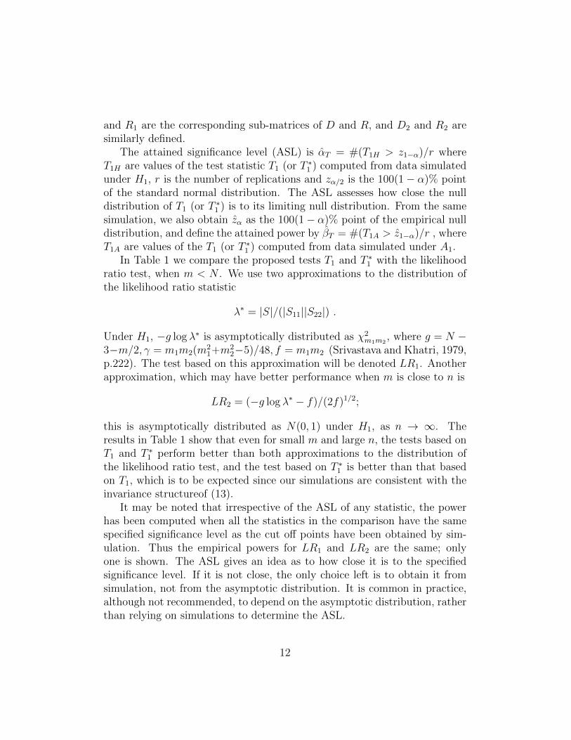
In Table 1 we compare the proposed tests T1 and T ∗1 with the likelihoodratio test, when m < N . We use two approximations to the distribution ofthe likelihood ratio statistic

λ∗ = |S|/(|S11||S22|) .

Under H1, −g log λ∗ is asymptotically distributed as χ2m1m2

, where g = N −3−m/2, γ = m1m2(m

21+m2

2−5)/48, f = m1m2 (Srivastava and Khatri, 1979,p.222). The test based on this approximation will be denoted LR1. Anotherapproximation, which may have better performance when m is close to n is

LR2 = (−g log λ∗ − f)/(2f)1/2;

this is asymptotically distributed as N(0, 1) under H1, as n → ∞. Theresults in Table 1 show that even for small m and large n, the tests based onT1 and T ∗1 perform better than both approximations to the distribution ofthe likelihood ratio test, and the test based on T ∗1 is better than that basedon T1, which is to be expected since our simulations are consistent with theinvariance structureof (13).

It may be noted that irrespective of the ASL of any statistic, the powerhas been computed when all the statistics in the comparison have the samespecified significance level as the cut off points have been obtained by sim-ulation. Thus the empirical powers for LR1 and LR2 are the same; onlyone is shown. The ASL gives an idea as to how close it is to the specifiedsignificance level. If it is not close, the only choice left is to obtain it fromsimulation, not from the asymptotic distribution. It is common in practice,although not recommended, to depend on the asymptotic distribution, ratherthan relying on simulations to determine the ASL.

12

Szekely et al. (2009) proposed a nonparametric test for independence;the p-value for their test statistic is estimated by using the permutationdistribution. Limited simulations, not shown here, indicated that comparedto the test based on T1 or T ∗1 , their test has size closer to nominal, althoughslightly less power, for N < m, and much lower power for N > m.

3. Testing intraclass correlation

3.1. The test statistic

In this section, we consider the problem of testing that the covariancematrix Σ has the intraclass correlation structure,

Σ = τ 2[(1− ρ)Im + ρ1m1′m], −1/(m− 1) < ρ < 1 . (23)

When Σ is of the form (3.1), from (1.5) we can write

Ω =

(Ω11 Ω′12Ω12 Ω22

)=

(λ2 00 σ2Im−1

), (24)

where λ2 = τ 2[1+(m−1)ρ] > 0, and σ2 = τ 2(1−ρ). Thus, we can re-expressH2 as

H2 : Ω11 = λ2, Ω12 = 0, Ω22 = σ2Im−1, σ2 > 0.

When n > m, the maximum likelihood estimate of Ω11 under A2 remains thesame as the maximum likelihood estimate of λ2 under H2, since both Ω11

and λ2 are unknown scalars. Thus H2 is equivalent to

H2 : Ω12 = 0, Ω22 = σ2Im−1, σ2 > 0 ,

with Ω11 a nuisance parameter in both H2 and A2. Under H2 we note that

σ2 = tr(Ω22)/(m− 1) ≡ a∗1(2) .

We also define

a∗2(1) =Ω2

11

m− 1, a∗2(2) =

tr(Ω222)

m− 1, a∗(1,2) =

Ω′12Ω12

m− 1, (25)

and make the following assumption:Assumption B:

13

Table 1: Attained significance level and attained power of the tests of Σ12 = 0 based onT1 and T ∗

1 given in (12) and (18), compared to two versions of the likelihood ratio test.The covariance matrix is constructed from D = diag(di) where di = 2+(m− i+1)/m.Thelikelihood ratio test can only be used when m < N . These tables are based on 1,000simulations; additional runs with 10,000 simulations for several cases gave very similarresults.

ASL under H1 Power (ρ = 0.2)N m1 m2 T1 T ∗1 LR1 LR2 T1 T ∗1 LR1 LR2

2 3 0.064 0.056 0.024 0.033 0.169 0.191 0.060 0.0765 5 0.075 0.064 0.019 0.027 0.235 0.217 0.034 0.04210 15 0.054 0.055 — — 0.373 0.347 — —

15 50 50 0.056 0.054 — — 0.612 0.595 — —50 100 0.051 0.054 — — 0.651 0.606 — —100 200 0.049 0.047 — — 0.704 0.675 — —200 300 0.055 0.059 — — 0.710 0.671 — —400 600 0.047 0.047 — — 0.745 0.733 — —2 3 0.059 0.054 0.034 0.059 0.315 0.343 0.151 0.1935 5 0.069 0.069 0.028 0.069 0.389 0.362 0.081 0.10210 15 0.067 0.066 — — 0.626 0.597 — —50 50 0.057 0.050 — — 0.845 0.852 — —

25 50 100 0.051 0.044 — — 0.891 0.882 — —100 200 0.071 0.066 — — 0.917 0.913 — —200 300 0.061 0.058 — — 0.909 0.904 — —400 600 0.066 0.067 — — 0.916 0.914 — —2 3 0.061 0.060 0.037 0.056 0.530 0.528 0.298 0.3565 5 0.054 0.056 0.035 0.042 0.780 0.782 0.324 0.35310 15 0.058 0.061 0.061 0.037 0.929 0.921 0.135 0.148

50 50 50 0.048 0.0571 — — 0.994 0.996 — —50 100 0.042 0.049 — — 0.999 0.998 — —100 200 0.059 0.058 — — 0.999 0.999 — —200 300 0.068 0.065 — — 0.999 0.999 — —400 600 0.061 0.059 — — 0.999 0.998 — —2 3 0.068 0.056 0.045 0.065 0.848 0.841 0.705 0.7505 5 0.058 0.064 0.039 0.055 0.972 0.972 0.746 0.77310 15 0.061 0.060 0.036 0.045 0.998 0.998 0.518 0.54250 50 0.051 0.045 — — 1 1 — —

100 50 100 0.064 0.061 — — 1 1 — —100 200 0.044 0.044 — — 1 1 — —200 300 0.060 0.059 — — 1 1 — —400 600 0.059 0.059 — — 1 1 — —14

Table 2: Attained significance level and attained power of the tests of Σ12 = 0 based onT1 and T ∗

1 given in (12) and (18), compared to two versions of the likelihood ratio test.The covariance matrix is constructed from D = diag(di) where di ≈ χ2

3. The likelihoodratio test can only be used when m < N . These tables are based on 1,000 simulations.

ASL under H1 Power (ρ = 0.2)N m1 m2 T1 T ∗1 LR1 LR2 T1 T ∗1 LR1 LR2

2 3 0.074 0.075 0.032 0.047 0.096 0.149 0.058 0.0815 5 0.055 0.047 0.020 0.024 0.124 0.276 0.035 0.04510 15 0.060 0.056 — — 0.141 0.385 — —

15 50 50 0.063 0.047 — — 0.188 0.585 — —50 100 0.064 0.047 — — 0.201 0.640 — —100 200 0.059 0.061 — — 0.258 0.625 — —200 300 0.038 0.051 — — 0.454 0.677 — —400 600 0.058 0.050 — — 0.480 0.712 — —2 3 0.065 0.048 0.028 0.038 0.202 0.312 0.129 0.1685 5 0.080 0.054 0.024 0.031 0.234 0.464 0.102 0.12110 15 0.072 0.052 — — 0.229 0.613 — —50 50 0.069 0.051 — — 0.344 0.844 — —

25 50 100 0.060 0.050 — — 0.479 0.858 — —100 200 0.054 0.056 — — 0.608 0.899 — —200 300 0.060 0.0548 — — 0.685 0.935 — —400 600 0.072 0.060 — — 0.682 0.910 — —2 3 0.066 0.066 0.044 0.055 0.250 0.504 0.325 0.3905 5 0.059 0.063 0.039 0.046 0.487 0.768 0.322 0.36610 15 0.057 0.058 0.035 0.039 0.782 0.931 0.152 0.164

50 50 50 0.062 0.056 — — 0.631 0.993 — —50 100 0.054 0.066 — — 0.837 0.996 — —100 200 0.052 0.062 — — 0.956 0.996 — —200 300 0.050 0.053 — — 0.969 0.999 — —400 600 0.055 0.055 — — 0.964 0.998 — —2 3 0.073 0.069 0.047 0.060 0.662 0.826 0.700 0.7505 5 0.073 0.060 0.049 0.060 0.704 0.974 0.732 0.76810 15 0.061 0.060 0.036 0.045 0.739 0.999 0.532 0.55050 50 0.070 0.062 — — 0.997 1 — —

100 50 100 0.068 0.057 — — 0.992 1 — —100 200 0.060 0.055 — — 0.997 1 — —200 300 0.069 0.064 — — 1 1 — —400 600 0.068 0.067 — — 1 1 — —

15

(i) 0 < limm→∞ a∗i(2) <∞, i = 1, 2,

(ii) 0 ≤ limm→∞ a∗(1,2) <∞,

(iii) n = O(mδ), δ > 0.

The parameters

F1 =a∗(1,2)√

2a∗2(1)a∗2(2)

and F2 =1

2

(1−

a∗21(2)a∗2(2)

), (26)

are invariant under the group of transformations

x→(c1 0′

0 c2Gm−1

)x , (27)

where Gm−1 is orthogonal and ci > 0, i = 1, 2. We consider a distancefunction that measures the difference between the hypothesis H2 and thealternative hypothesis A2 : Σ > 0. Let D be an m×m diagonal matrix givenby

D = diag

[1

2(2a∗2(1))

− 12 ,

1

2(a∗2(2))

− 12 Im−1

]= diag (d1, d2Im−1) .

We define a distance that measures the difference between the hypothesis H2

and A2 by

η2 =1

(m− 1)tr

[D

(Ω11 Ω′12Ω12 Ω22

)−D

(Ω11 00 a∗1(2)Im−1

)]2=

1

(m− 1)tr

[D

(0 Ω′12

Ω12

(Ω22 − a∗1(2)Im−1

) )]2

=1

(m− 1)tr

(0 d1Ω

′12

d2Ω12 d2

(Ω22 − a∗1(2)Im−1

) )2

=a∗(1,2)√

2a∗2(1)a∗2(2)

+1

2

[1− a∗21(2)a∗2(2)

]= F1 + F2

16

It may be noted that η2 = 0 if and only if H2 holds, otherwise η2 > 0. Thus,a test statistic based on a consistent estimator of η2 can be proposed.

We consider tests based on the sample covariance matrix S = n−1V , orequivalently on the m × m matrix W = GV G′ ∼ Wm(Ω, n), Ω = GΣG′,where G has the Helmert form described at (4), and W is partitioned toconform with the partition of Ω at (24).

The following results from Srivastava and Khatri (1979, p.80) hold whethern < m or n ≥ m:

(i) W2.1 = W22 −W−111 W 12W

′12 ∼ Wm−1(Ω2.1, n− 1)

is independently distributed of (W 12,W11)

(ii) W 12 given W11 ∼ Nm−1(βW11,W11Ω2.1) ,

(iii) W11 ∼ Ω11χ2n ,

whereβ = Ω−111 Ω12, and Ω2.1 = Ω22 − Ω−111 Ω12Ω

′12 .

We define

a∗(1,2) =1

(n− 1)(n+ 2)(m− 1)

[W ′

12W 12 −1

nW11 tr(W22)

], (28)

a∗1(2) =tr(W22)

n(m− 1), a∗1(1) =

W11

n(m− 1), (29)

a∗2(1) =W 2

11

(n− 1)(n+ 2)(m− 1), (30)

a∗2(2) =1

(n− 1)(n+ 2)(m− 1)

[tr(W 2

22)−1

ntr(W22)2

]. (31)

We propose the statistic

T2 =n√2

(F1 + F2

), (32)

where

F1 =a∗(1,2)√

2a∗2(1)a∗2(2)

= [(n− 1)(n+ 2)(m− 1)]1/2a∗(1,2)√

2a∗2(2)W11

(33)

, F2 =1

2

(1−

a∗21(2)a∗2(2)

), (34)

17

for testing the hypothesis H2 against the alternative A2. The statistic T2 isinvariant under the transformation:

W →(c1 00 c2Im−1

)W

(c1 00 c2Im−1

).

Hence, without any loss of generality, we may assume that the matrix Ω = Iwhen obtaining the distribution of T2 under the hypothesisH2 and calculatingits average significance level (ASL) or power; see the discussion of Tables 3and 4 below.

3.2. Asymptotic null distribution of T2Under H2,W ∼ Wm(Ω, n), where Ω = diag(λ2, σ2Im−1). Hence, we can

write W = (z1, Z2)′(z1, Z2), and

W = (z1, . . . ,zm)′(z1, . . . ,zm) =

(W11 W ′

12

W 12 W22

), (35)

where zi are independently distributed with z1 ∼ Nn(0, λIn) and z2, . . . ,zm ∼Nn(0, σ2In). Also W11 = z′1z1, W

′12 = z′1Z2, W22 = Z ′2Z2 . Hence,

na∗(1,2)√a∗2(1)

=1

(m− 1)1/2(z′1z1)

[z′1Z2Z

′2z1 −

1

n(z′1z1)tr(Z2Z

′2)

]

=σ2

(m− 1)1/2

m∑j=2

[(z′1zj)

2

σ2(z′1z1)− 1

nσ2(z′jzj)

]

By the law of large numbers, (nσ2)−1(z′jzj)p→ 1 as n→∞. Given z1, z

′1zj/σ(z′1z1)

1/2

is standard normal, so [(z′1zj)

2/σ2(z′1z1)]

is distributed as χ21, independently of z1. From Slutzky’s theorem and the

central limit theorem,

na∗(1,2)

σ2√

2a∗2(1)

=1

(m− 1)1/2

m∑j=2

1√2

[(z′1zj)

2

σ2(z′1z1)− 1

nσ2(z′jzj)

]→ N(0, 1) , (36)

as (m,n)→∞. A consistent estimator of σ2 is given by a∗1/22(2) . Hence, we get

the following theorem.

18

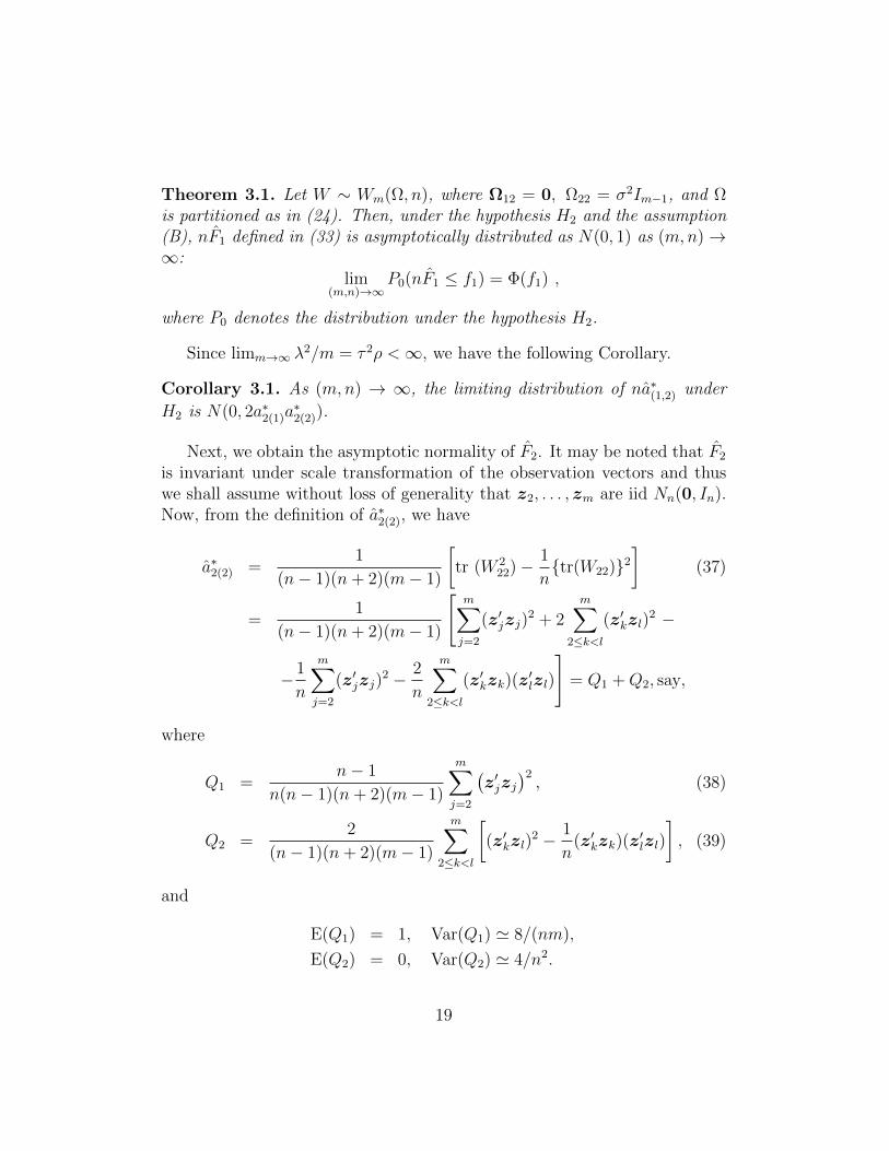
Theorem 3.1. Let W ∼ Wm(Ω, n), where Ω12 = 0, Ω22 = σ2Im−1, and Ωis partitioned as in (24). Then, under the hypothesis H2 and the assumption(B), nF1 defined in (33) is asymptotically distributed as N(0, 1) as (m,n)→∞:

lim(m,n)→∞

P0(nF1 ≤ f1) = Φ(f1) ,

where P0 denotes the distribution under the hypothesis H2.

Since limm→∞ λ2/m = τ 2ρ <∞, we have the following Corollary.

Corollary 3.1. As (m,n) → ∞, the limiting distribution of na∗(1,2) under

H2 is N(0, 2a∗2(1)a∗2(2)).

Next, we obtain the asymptotic normality of F2. It may be noted that F2

is invariant under scale transformation of the observation vectors and thuswe shall assume without loss of generality that z2, . . . ,zm are iid Nn(0, In).Now, from the definition of a∗2(2), we have

a∗2(2) =1

(n− 1)(n+ 2)(m− 1)

[tr (W 2

22)−1

ntr(W22)2

](37)

=1

(n− 1)(n+ 2)(m− 1)

[m∑j=2

(z′jzj)2 + 2

m∑2≤k<l

(z′kzl)2 −

− 1

n

m∑j=2

(z′jzj)2 − 2

n

m∑2≤k<l

(z′kzk)(z′lzl)

]= Q1 +Q2, say,

where

Q1 =n− 1

n(n− 1)(n+ 2)(m− 1)

m∑j=2

(z′jzj

)2, (38)

Q2 =2

(n− 1)(n+ 2)(m− 1)

m∑2≤k<l

[(z′kzl)

2 − 1

n(z′kzk)(z

′lzl)

], (39)

and

E(Q1) = 1, Var(Q1) ' 8/(nm),

E(Q2) = 0, Var(Q2) ' 4/n2.

19

It follows from the central limit theorem that as (m,n)→∞

√mn

(Q1

σ4− 1

)d→ N(0, 8),

where now we give the result for general σ2.To find the distribution of Q2, let

ηj =2

n(m− 1)

j−1∑i=2

[(z′izj)

2 − 1

n(z′izi)(z

′jzj)

], j = 3, . . . ,m− 1 (40)

ThenE(ηj|Fj−1) = 0, and E(η2j |Fj−1) <∞ .

where Fj is the σ-algebra generated by the random vectors z2, . . . ,zj. Let-ting z1 = 0, and F1 = (∅,X ), where Φ is the empty set, and X is the wholespace, we find that F1 ⊂ F2 ⊂, . . . ,⊂ Fm ⊂ F , and ηj,Fj is a sequence ofintegrable martingale differences. We note that

nQ2 'm∑j=3

ηj . (41)

We need to show that the Lindeberg condition

L =m∑j=3

E[η2j I(|ηj| > ε) | Fj−1

] p→ 0

is satisfied. From Markov’s inequality and the Cauchy-Schwarz inequality,as in the Appendix, we have

P (L > ξ) ≤m∑j=3

E(η4j)/ε2ξ.

As in §2, write

uij = (z′izj)2 − 1

n(z′izi)

(z′jzj

).

Then, it can be shown that

n4(m− 1)4m∑j=3

E(η4j)

= 16m∑j=3

E

(j−1∑i=2

u4ij + 6

j−1∑2≤k<l

u2kju2il

)= O

(m3n4

).

20

Thus, the Lindeberg condition is satisfied. We now show that

M =m∑j=3

E(η2j |Fj−1)p→ 4, and Var(M)→ 0.

The variance of M is

V2 = Var

[4

n2(m− 1)2

m∑j=3

(j−1∑i=2

b(j)in + 2

j−1∑2≤k<l

c(j)kln

)],

whereb(j)in = E(u2ij | Fj−1), c

(j)kln = E(uklulj | Fj−1).

It can be shown that

E

[m∑j=3

E(η2j | Fj−1)

]=

m∑j=3

E(η2j ) ' 4 .

As well,

Var

[4

n2(m− 1)2

m∑j=3

m−1∑i=2

b(j)in

]= O(m−1n−2) , and

Var

[8

n2(m− 1)2

m∑j=3

∑2≤k<l

c(j)kln

]= O(m−1n−2), so V2 → 0.

Hence, from Theorem 4 of Shiryayev (1984), as (m,n) → ∞, the limitingdistribution of nQ2 is N(0, 4). Next, we consider the joint distribution ofa∗1(2) and Q1, where

a∗1(2) =

∑mj=2(z

′jzj)

n(m− 1)and Q1

d=

n− 1

n2(m− 1)

m∑j=2

(z′jzj)2 .

As before, σ2 will be assumed to be one. Let ε1i = (z′izi − n) /√n, ε2i =

[(z′izi)2 − n(n + 2)] /

√n(n+ 2)(n+ 3) , i = 2, ...,m . Then E(ε1i) =

0, Var(ε1i) = 1, E(ε2i) = 0, Var(ε2i) = 1, and Cov(ε1i, ε2i) = 4δn, δn =√(n+ 2)/(n+ 3). The bivariate random vectors (ε1i, ε2i)

′ are independentand identically distributed with mean vector 0, and finite covariance matrix,

21

i = 2, . . . ,m. Hence, from the multivariate central limit theorem, it followsthat as (m,n)→∞ , in any manner,

√mn

(a∗1(2)Q1

)d→ N2

[(11

),

(2 44 8

)]It can easily be shown that Cov(a∗1(2), Q2) = 0. Now we apply Lemma A.1 in

the Appendix to conclude that a∗(1,2), a∗1(2)and a∗2(2) defined in (3.6) – (3.9) are

jointly normal. From this, it follows that a∗(1,2) and (a∗1(2), a∗2(2)) are asymptot-

ically independently distributed under H2. Since a∗2(2)p→ σ4 and a∗2(1)

p→ λ2, it

follows that F1 and F2 are asymptotically independently distributed. To findthe distribution of F2, we apply the delta method to the joint distribution ofa∗1(2) and a∗2(2), using

∂F2

∂a∗1(2)=

2a∗1(2)a∗2(2)

, and∂F2

∂a∗2(2)= −

a∗21(2)a∗22(2)

,

and

(2,−1)

(2nm

4nm

4nm

8nm

+ 4n2

)(2−1

)=

(0,− 4

n2

)(2−1

)=

4

n2.

Hence, as (m,n)→∞, (n/2)F2d→ N(0, 1), and we have the following:

Theorem 3.2. Let W ∼ Wm(Ω, n), where Ω12 = 0, Ω22 = σ2Im−1, Ω11 =

λ2, and limm→∞(λ2/m) < ∞. Then under H2 and assumption B, T2d→

N(0, 1), as m and n →∞ .

3.3. Power of the test T2 and its attained significance level

As in §2, we examine attained significance level (ASL) first. Since thestatistic T2 is invariant under scale transformations of the first componentand the remaining (m − 1) components, we shall assume without loss ofgenerality that Ω = GΣG′ = Im. For the alternative, we consider Ω =DRD, D = diag(d1, . . . , dm), di = 2 + (m − i + 1)/m, R = (rij), where

rii = 1, rij = (−1)i+j(ρ)|i−j|0.1

. . The ASL and power are defined in the samemanner as in §2.3.

We compare the performance of T2 with that of the likelihood ratio statis-tic

λ∗ =|W2.1|

[tr(W22)/(m− 1)]m−1,

22

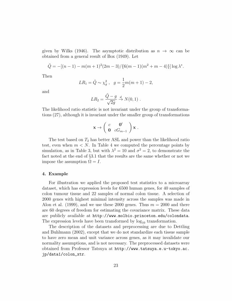
given by Wilks (1946). The asymptotic distribution as n → ∞ can beobtained from a general result of Box (1949). Let

Q = −[(n− 1)−m(m+ 1)2(2m− 3)/6(m− 1)(m2 +m− 4)] log λ∗.

Then

LR1 = Q ∼ χ2g , g =

1

2m(m+ 1)− 2,

and

LR2 =Q− g√

2g

d→ N(0, 1) .

The likelihood ratio statistic is not invariant under the group of transforma-tions (27), although it is invariant under the smaller group of transformations

x→(c 0′

0 cGm−1

)x .

The test based on T2 has better ASL and power than the likelihood ratiotest, even when m < N . In Table 4 we computed the percentage points bysimulation, as in Table 3, but with λ2 = 10 and σ2 = 2, to demonstrate thefact noted at the end of §3.1 that the results are the same whether or not weimpose the assumption Ω = I.

4. Example

For illustration we applied the proposed test statistics to a microarraydataset, which has expression levels for 6500 human genes, for 40 samples ofcolon tumour tissue and 22 samples of normal colon tissue. A selection of2000 genes with highest minimal intensity across the samples was made inAlon et al. (1999), and we use these 2000 genes. Thus m = 2000 and thereare 60 degrees of freedom for estimating the covariance matrix. These dataare publicly available at http://www.molbio.princeton.edu/colondata.The expression levels have been transformed by log10 transformation.

The description of the datasets and preprocessing are due to Dettlingand Buhlmann (2002), except that we do not standardize each tissue sampleto have zero mean and unit variance across genes, as it may invalidate ournormality assumptions, and is not necessary. The preprocessed datasets wereobtained from Professor Tatsuya at http://www.tatsuya.e.u-tokyo.ac.

jp/data1/colon_xtr.

23

Table 3: Attained significance level and attained power of the test of intraclass correlationbased on T2 given in (32), compared to two versions of the likelihood ratio test. Thecovariance matrix under H2 is the identity. The likelihood ratio test can only be usedwhen m < N . The number of simulations is 10,000.

ASL Under H Power (ρ=0.4)N m T2 LR1 LR2 T2 LR1

5 0.0408 0.0287 0.0262 0.6209 0.486620 0.0457 — — 0.9513 —

15 50 0.0450 — — 0.9934 —75 0.0464 — — 0.9971 —100 0.0464 — — 0.9988 —200 0.0467 — — 0.9999 —5 0.0404 0.0382 0.0345 0.8985 0.817420 0.0469 0.1683 0.1251 0.9988 0.9370

25 50 0.0470 — — 0.9999 —75 0.0447 — — 1 —100 0.0448 — — 1 —200 0.0468 — — 1 —5 0.0419 0.0445 0.0398 0.9975 0.994420 0.0533 0.0425 0.0504 1 1

50 50 0.0492 — — 1 —75 0.0461 — — 1 —100 0.0493 — — 1 —200 0.0474 — — 1 —5 0.0455 0.0457 0.0412 1 120 0.0503 0.0415 0.0456 1 1

100 50 0.0469 0.0922 0.0663 1 175 0.0486 0.7705 0.6772 1 1100 0.0487 — — 1 —200 0.0501 — — 1 —

24

Table 4: Attained significance level and attained power of the test of intraclass correlationbased on T2 given in (32), compared to two versions of the likelihood ratio test. Thecovariance matrix under H2 is the matrix at (24) with λ2 = 10 and σ2 = 2. The likelihoodratio test can only be used when m < N . The number of simulations is 10,000.

ASL Under H Power (ρ=0.2)N m T2 LR1 LR2 T2 LR1

5 0.0368 0.0289 0.0261 0.1679 0.124520 0.0446 — — 0.4546 —

15 50 0.0447 — — 0.6695 —75 0.0429 — — 0.7741 —100 0.0449 — — 0.8163 —200 0.0474 — — 0.9111 —5 0.0380 0.0385 0.0350 0.3116 0.245620 0.0447 0.1637 0.1288 0.7645 0.3122

25 50 0.0483 — — 0.9334 —75 0.0472 — — 0.9708 —100 0.0438 — — 0.9876 —200 0.0463 — — 0.9975 —5 0.0382 0.0442 0.0392 0.6664 0.597220 0.0447 0.0409 0.0475 0.9912 0.9554

50 50 0.0495 — — 1 —75 0.0449 — — 1 —100 0.0492 — — 1 —200 0.0453 — — 1 —5 0.0412 0.0502 0.0434 0.9635 0.944920 0.0506 0.0409 0.0479 1 1

100 50 0.0507 0.0863 0.0615 1 175 0.0492 0.7640 0.6741 1 1100 0.0494 — — 1 —200 0.0451 — — 1 —

25

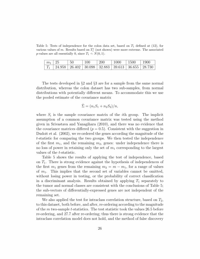
Table 5: Tests of independence for the colon data set, based on T1 defined at (12), forvarious values of m. Results based on T ∗

1 (not shown) were more extreme. The associatedp-values are all essentially 0, since T1

.∼ N(0, 1).

m1 25 50 100 200 1000 1500 1900T1 24.958 26.402 30.098 32.883 39.613 36.655 28.730

The tests developed in §2 and §3 are for a sample from the same normaldistribution, whereas the colon dataset has two sub-samples, from normaldistributions with potentially different means. To accommodate this we usethe pooled estimate of the covariance matrix

Σ = (n1S1 + n2S2)/n,

where Si is the sample covariance matrix of the ith group. The implicitassumption of a common covariance matrix was tested using the methodgiven in Srivastava and Yanagihara (2010), and there was no evidence thatthe covariance matrices differed (p = 0.5). Consistent with the suggestion inDudoit et al. (2002), we re-ordered the genes according the magnitude of thet-statistic for comparing the two groups. We then tested the independenceof the first m1, and the remaining m2, genes: under independence there isno loss of power in retaining only the set of m1 corresponding to the largestvalues of the t-statistic.

Table 5 shows the results of applying the test of independence, basedon T1. There is strong evidence against the hypothesis of independences ofthe first m1 genes from the remaining m2 = m −m1, for a range of valuesof m1. This implies that the second set of variables cannot be omitted,without losing power in testing, or the probability of correct classificationin a discriminant analysis. Results obtained by applying T1 separately tothe tumor and normal classes are consistent with the conclusions of Table 5;the sub-vectors of differentially-expressed genes are not independent of theremaining set.

We also applied the test for intraclass correlation structure, based on T2,to this dataset, both before, and after, re-ordering according to the magnitudeof the m two-sample t-statistics. The test statistic took the values 26.5 beforere-ordering, and 27.7 after re-ordering; thus there is strong evidence that theintraclass correlation model does not hold, and the method of false discovery

26

rates should no be applied for this dataset.

5. Concluding Remarks

In this paper, we propose test statistics for testing independence, as wellas for testing intraclass correlation structure, based on consistent estimatorsof the distance function between the hypothesis and the alternative. We havecompared the attained significance level with the nominal level α = 0.05. Itseems that the asymptotic null distributions provide good approximationsto the significance level, and the power of the tests are excellent. It may benoted that the proposed tests are valid for both m < N and m > N , andcan thus be recommended over the likelihood ratio test, which can only beused when m < N . Particularly when m is close to N , results in Tables 1and 2 indicate that the likelihood ratio test can have very poor power.

Appendix

In §2 and §3 we used invariance arguments and a central limit theoremfor independent but not identically distributed random variables. In thisappendix we present these results in general notation.

Assume that the sample of n observations x, i = 1, . . . , n are indepen-dent and identically distributed with mean 0 and positive definite covari-ance matrix Σ. Since n < m, the sample covariance matrix S as well asV = nS are singular. Consider two sample points X = (x1, . . . ,xn) andX∗ = (x∗1, . . . ,x

∗n) and let

Z = (X,X1) and Z∗ = (X∗, X∗1 )

where X1 and X∗1 are both m× (m− n) matrices of arbitrary values so thatthe m×m matrices Z and Z∗ are nonsingular. Let Ir denote the r×r identitymatrix. Then,

Im = (Z∗)−1Z∗ = (Z∗)−1(X∗, X∗1 )

=[(Z∗)−1X∗, (Z∗)−1X∗1

]=

(In 00 Im−n

).

Hence,

(Z∗)−1X∗ =

(In0

), and Z(Z∗)−1X∗ = (X,X1)

(In0

)= X,

27

and X = AX∗, A = Z(Z∗)−1, where A is nonsingular. Thus for any twopoints, there exists a nonsingular matrix taking one to the other; i.e. thewhole space is a single orbit. This implies that the group of nonsingulartransformations is transitive, and no invariant statistic exists.

For example, for testing the independence of two subvectors x1 and x2

where x′ = (x′1,x′2), no invariant test exists under the nonsingular group of

transformation

x→(A1 00 A2

)x ,

where A1 and A2 are m1×m1 and m2×m2, m1 +m2 = m are non singularmatrices. For this reason we consider in §2 and §3 the more restricted groupof transformations given at (2.1) and (3.5).

We now give a lemma to establish the joint asymptotic normality of thek statistics

t(n)i,m =

m∑j=1

x(n)ij , i = 1, ..., k.

where x(n)ij is a sequence of random variables which may depend on n. We

consider an arbitrary linear combination of these k statistics, namely,

t(n)m = c1t(n)1,m + ...+ ckt

(n)k,m =

m∑j=1

k∑i=1

cix(n)ij ≡

m∑j=1

y(n)j

where without any loss of generality, we assume that c21 + ...+ c2k = 1. Fromthe definition of multivariate normality, see Srivastava and Khatri (1979,

p. 43), joint normality of t(n)im , i = 1, ..., k, will follow if the normality of

t(n)m is established for all c1, . . . , ck . Let F (n)

` be the σ-algebra generated

by the random variables (x(n)1j , . . . , x

(n)kj ), j = 1, ..., `, ` = 1, ...,m. Then

F0 ⊂ F (n)1 ⊂ ... ⊂ F (n)

m ⊂ F , where (Ω,F , P ) is the probability space,F0 = ∅,Ω, ∅ is the null set and Ω is the whole space.

Lemma A.1 Let x(n)ij be a sequence of random variables, y

(n)j =

∑ki=1 cix

(n)ij ,

i = 1, . . . , k, j = 1, . . . ,m, and n = O(mδ), δ > 0. We assume that

(i) E(y(n)j | F

(n)j−1) = 0,

(ii) lim(n,m)→∞

E[(y(n)j )2] <∞,

28

(iii)m∑j=0

E[(y(n)j )2 | F (n)

j−1]p−→ σ2

0, as(n,m)→∞,

(iv) L ≡∑m

j=0E[(y(n)j )2 I(|y(n)j | > ε) | F (n)

j−1]p−→ 0, as (n,m)→∞,

Then

t(n)m =m∑j=1

y(n)j

d→ N(0, σ20), as (n,m)→∞.

The proof of this lemma follows from Theorem 4 of Shiryayev (1984, p. 511),

since the first two conditions imply that x(n)j ,F (n)j forms a sequence of in-

tegrable martingale differences. Condition (iv) is known as Lindeberg’s con-dition. To verify this condition, we note that from the Markov and Cauchy-Schwarz inequalities

P [L > δ] ≤m∑j=0

E[(y(n)j )2I(|y(n)j | > ε]/δ

≤m∑j=0

E[(y(n)j )4]/δε2 .

We also know that

E[(y(n)j )4] ≤ k3

k∑i=1

c4iE[(x(n)ij )4].

Hence, if∑m

j=0E[(x(n)ij )4]→ 0, for all i = 1, ..., k, the Lindeberg condition is

satisfied. It is rather simple to evaluate σ20 in most cases.

References

Alon, U., Barkai, N. Motterman, D. Gish, K., Mack, S. and Levine, J. (1999).Broad patterns of gene expression revealed by clustering analysis of tumorand normal colon tissues probed by oligonucleotide arrays. Proc. Nat. Acad.Sci. 96, 6745–6750.

Benjamini, Y. and Hochberg, Y. (1995). Controlling the false discovery rate:a practical and power approach to multiple testing. J. R. Statist. Soc. B57, 289–300.

29

Benjamini, Y. and Yekutieli, D. (2001). The control of the false discoveryrate in multiple testing under dependency. Ann. Statist. 29, 1165–1181.

Box, G.E.P. (1949). A general distribution theory for a class of likelihoodcriteria. Biometrika 36, 317–346.

Dettling, M. and Buhlmann, P. (2002). Boosting for tumor classification withgene expression data. Bioinformatics 19, 1061–1069.

Dudoit, S., Fridlyand, J., and Speed, T. P. (2002). Comparison of discrimi-nation methods for the classification of tumors using gene expression data.J. Am. Statist. Assoc. 97, 77–87.

Golub, T., Slonim, D., Tamayo, P., Huard, C., Gaasenbeek, M., Mesirov,J., Coller, H., Loh, M. and Downing, J. (1999). Molecular classification ofcancer: class discovery and class prediction by gene expression monitoring.Science 296, 531–537.

Schott, J.R. (2005). Testing for complete independence in high dimensions.Biometrika 92, 951–956.

Shiryayev, A.N. (1984). Probability. Springer-Verlag, New York.

Srivastava, M.S. (2005). Some tests concerning the covariance matrix in high-dimensional data. J. Japan Stat. Soc. 35, 251–272.

Srivastava, M.S. (2006). Some test criteria for the covariance matrix withfewer observations than the dimension. Acta et Commentations Universi-tatis Tartuensis de Mathematica 10, 77–93.

Srivastava, M.S., and Khatri, C.G. (1979). An Introduction to MultivariateStatistics. North-Holland, New York.

Srivastava, M.S. and Yanagihara, H. (2010). Testing the equality of severalcovariance matrices with fewer observations than the dimension. J. Mult.Anal. 101, 1310–1329.

Szekely, G.J. and Rizzo, M.L. (2009). Brownian distance covariance. Ann.Appl. Statist. 3, 1236–1265.

Wilks, S.S.(1946). Sample criteria for testing equality of means, equality ofvariances, and equality of covariances in a normal multivariate distribution.Ann. Statist. 17, 257–281.

30