arX

iv:m

ath/

0701

124v

1 [

mat

h.ST

] 4

Jan

200

7

High Dimensional Covariance Matrix Estimation

Using a Factor Model ∗

By Jianqing Fan, Yingying Fan and Jinchi Lv

Princeton University

August 12, 2006

High dimensionality comparable to sample size is common in many statis-

tical problems. We examine covariance matrix estimation in the asymptotic

framework that the dimensionality p tends to ∞ as the sample size n in-

creases. Motivated by the Arbitrage Pricing Theory in finance, a multi-factor

model is employed to reduce dimensionality and to estimate the covariance

matrix. The factors are observable and the number of factors K is allowed

to grow with p. We investigate impact of p and K on the performance of the

model-based covariance matrix estimator. Under mild assumptions, we have

established convergence rates and asymptotic normality of the model-based

estimator. Its performance is compared with that of the sample covariance

matrix. We identify situations under which the factor approach increases

performance substantially or marginally. The impacts of covariance matrix

estimation on portfolio allocation and risk management are studied. The

asymptotic results are supported by a thorough simulation study.

Short Title: Large Covariance Matrix Estimation.

AMS 2000 subject classifications. Primary 62F12, 62H12; secondary 62J05, 62E20.

Key words and phrases. Factor model, diverging dimensionality, covariance matrix

estimation, consistency, asymptotic normality, optimal portfolio, risk management.

∗Financial support from the NSF under grant DMS-0532370 is gratefully acknowledged. Address

for correspondence: Jinchi Lv, Department of Mathematics, Princeton University, Princeton, NJ 08544.

Phone: (609) 258-9433. E-mail: jlv@princeton.edu.

1

1. Introduction.

1.1. Background. Covariance matrix estimation is fundamental for almost all areas

of multivariate analysis and many other applied problems. In particular, covariance ma-

trices and their inverses play a central role in risk management and portfolio allocation.

For example, the smallest and largest eigenvalues of a covariance matrix are related to

the minimum and maximum variances of the selected portfolio, respectively, and the

eigenvectors are related to portfolio allocation. Therefore, we need a good covariance

matrix estimator inverting which does not excessively amplify the estimation error. See

Goldfarb and Iyengar (2003) for applications of covariance matrices to portfolio selec-

tions and Johnstone (2001) for their statistical implications.

Estimating high-dimensional covariance matrices is intrinsically challenging. For

example, in portfolio allocation and risk management, the number of stocks p, which is

typically of the same order as the sample size n, can well be in the order of hundreds.

In particular, when p = 200 there are more than 20,000 parameters in the covariance

matrix. Yet, the available sample size is usually in the order of hundreds or a few

thousands because longer time series (larger n) increases modeling bias. For instance,

by taking daily data of the past three years we have only roughly n = 750. So it is hard

or even unrealistic to estimate covariance matrices without imposing any structure (see

the rejoinder in Fan, 2005).

Factor models have been widely used both theoretically and empirically in economics

and finance. Derived by Ross (1976, 1977) using the Arbitrage Pricing Theory (APT)

and by Chamberlain and Rothschild (1983) in a large economy, the multi-factor model

states that the excessive return of any asset Yi over the risk-free interest rate satisfies

(1.1) Yi = bi1f1 + · · · + biKfK + εi, i = 1, · · · , p,

where f1, · · · , fK are the excessive returns of K factors, bij , i = 1, · · · , p, j = 1, · · · ,K,

are unknown factor loadings, and ε1, · · · , εp are p idiosyncratic errors uncorrelated given

f1, · · · , fK . In economics and finance literature, factors are implicitly assumed to be ob-

servable and there is a large literature contributed to construction of factors (e.g. Fama

and French, 1992, 1993). The factor models have been widely applied in economics and

finance. See, for example, Ross (1976, 1977), Engle and Watson (1981), Chamberlain

(1983), Chamberlain and Rothschild (1983), Diebold and Nerlove (1989), Fama and

French (1992, 1993), Aguilar and West (2000), and Stock and Watson (2005) and refer-

ences therein. These are extensions of the famous Capital Asset Pricing Model (CAPM)

and can be regarded as efforts to approximate the market portfolio in the CAPM.

2

Thanks to the multi-factor model (1.1), if a few factors can completely capture the

cross-sectional risks, the number of parameters in covariance matrix estimation can be

significantly reduced. For example, using the Fama-French three-factor model [Fama

and French (1992, 1993)], there are 4p instead of p(p+1)/2 parameters to be estimated.

Despite the popularity of factor models in the literature, the impact of dimensionality on

the estimation errors of covariance matrices and its applications to portfolio allocation

and risk management are poorly understood, so in this paper, determined efforts are

made on such an investigation. To make the multi-factor model more realistic, we allow

K to grow with the number of assets p and hence with the sample size n. As a result,

we also investigate the impact of the number of factors on the estimation of covariance

matrices, as well as its applications to portfolio allocation and risk management. To

appreciate the derived rates of convergence, we compare them with those without using

the factor structure. One natural candidate is the sample covariance matrix. This also

allows us to examine the impact of dimensionality on the performance of the sample

covariance matrix. Our results can also be regarded as an important step to understand

the performance of factor models with unobservable factors.

The factor model has been extensively studied in the literature [see, e.g. Scott (1966)

and (1969), Browne (1987), Browne and Shapiro (1987), and Yuan and Bentler (1997)],

but traditional work assumes the sample size n tends to infinity while the dimensionality

p and the number of factors K are fixed. There is a relatively small literature on studies

of models with a diverging number of parameters. See, for example, Huber (1973),

Yohai and Maronna (1979), Portnoy (1984, 1985), and Bai (2003). In particular, Fan

and Peng (2004) establish some asymptotic properties, as well as an oracle property,

for nonconcave penalized likelihood estimators in the presence of a diverging number of

parameters. One can further refer to seminal reviews by Donoho (2000) and Fan and Li

(2006) for challenges of high dimensionality. But it still remains open to examine factor

models with diverging dimensionality and growing number of factors for the purpose of

covariance matrix estimation.

The traditional covariance matrix estimator, the sample covariance matrix, is known

to be unbiased, and it is invertible when the dimensionality is no larger than the sample

size. See, for example, Eaton and Tyler (1991, 1994) for the asymptotic spectral distri-

butions of random matrices including sample covariance matrices and their statistical

implications. In the absence of prior information about the population covariance ma-

trix, the sample covariance matrix is certainly a natural candidate in the case of small

dimensionality, but no longer performs very well for moderate or large dimensionality

3

[see, e.g. Lin and Perlman (1985) and Johnstone (2001)]. Many approaches were pro-

posed in the literature to construct good covariance matrix estimators. Among them,

two main directions were taken. One is to remedy the sample covariance matrix and

construct a better one by using approaches such as shrinkage and the eigen-method,

etc. See, for example, Ledoit and Wolf (2004) and Stein (1975). The other one is to re-

duce dimensionality by imposing some structure on the data. Many structures, such as

sparsity, compound symmetry, and the autoregressive model, are widely used. Various

approaches were taken to seek a balance between the bias and variance of covariance

matrix estimators. See, for example, Dempster (1972), Leonard and Hsu (1992), Chiu,

Leonard and Tsui (1996), Diggle and Verbyla (1998), Pourahmadi (2000), Boik (2002),

Smith and Kohn (2002), Wong, Carter and Kohn (2003), Wu and Pourahmadi (2003),

Huang, Liu and Pourahmadi (2004), and Li and Gui (2005).

1.2. Covariance matrix estimation. We always denote by n the sample size, by p the

dimensionality, and by f1, · · · , fK the K observable factors, where p grows with sample

size n and K increases with dimensionality p. For ease of presentation, we rewrite factor

model (1.1) in matrix form

(1.2) y = Bnf + ε,

where y = (Y1, · · · , Yp)′, Bn = (b1, · · · ,bp)

′ with bi = (bn,i1, · · · , bn,iK)′, i = 1, · · · , p,f = (f1, · · · , fK)′, and ε = (ε1, · · · , εp)′. Throughout we assume that E(ε|f) = 0 and

cov(ε|f) = Σn,0 is diagonal. For brevity of notation, we suppress the first subscript n in

some situations where the dependence on n is self-evident.

Let (f1,y1), · · · , (fn,yn) be n independent and identically distributed (i.i.d.) samples

of (f,y). We introduce here some notation used throughout the paper. Let

Σn = cov(y), X = (f1, · · · , fn), Y = (y1, · · · ,yn) and E = (ε1, · · · , εn).

Under model (1.2), we have

(1.3) Σn = cov(Bnf) + cov(ε) = Bncov(f)B′n + Σn,0.

A natural idea for estimating Σn is to plug in the least-squares estimators of Bn, cov(f),

and Σn,0. Therefore, we have a substitution estimator

(1.4) Σn = Bncov(f)B′

n + Σn,0,

where Bn = YX′(XX′)−1 is the matrix of estimated regression coefficients, cov(f) =

(n − 1)−1XX′ − {n(n − 1)}−1X11′X′ is the sample covariance matrix of the factors f,

4

and

Σn,0 = diag(n−1EE

′)

is the diagonal matrix of n−1EE′

with E = Y − BX the matrix of residuals. If the

factor model is not employed, then we have the sample covariance matrix estimator

(1.5) Σsam = (n− 1)−1YY′ − {n (n− 1)}−1

Y11′Y′.

This paper mainly provides a theoretical understanding of the factor model with a

diverging dimensionality and growing number of factors for the purpose of covariance

matrix estimation; it does not aim to compare with other popular estimators. Through-

out the paper, we always contrast the performance of the covariance matrix estimator Σ

in (1.4) with that of the sample covariance matrix Σsam in (1.5). With prior information

of the true factor structure, the substitution estimator Σ is expected to perform better

than Σsam. However, this has not formally been shown, especially when p → ∞ and

K → ∞, and this is not always true. In addition, exact properties of this kind are not

well understood. As the problem is important for portfolio management, determined

efforts are devoted in regard to this. Our conclusion can be summarized as follows.

• Σ is always invertible, even if p > n, while Σsam suffers from the problem of

possibly being singular when dimensionality p is close to or larger than sample

size n.

• The advantage of the factor model lies in the estimation of the inverse of the

covariance matrix, not the estimation of the covariance matrix itself. When the

parameters involve the inverse of the covariance matrix, the factor model shows

substantial gains, whereas when the parameters involved the covariance matrix

directly, the factor model does not have much advantage. The latter is a surprise

to the conventional wisdom.

• Portfolio allocations involve the inverse of the covariance matrix and the factor-

model based estimates gain substantially, whereas the risk management involves

directly the covariance matrix and the gain is only marginally.

• Σ has asymptotic normality, while in general Σsam may not have asymptotic nor-

mality of the same kind.

These properties will be demonstrated in our paper as follows.

5

1.3. Outline of the paper. In section 2 we discuss some basic assumptions and present

the sampling properties of the estimator Σ, as well as those of Σsam. We study the im-

pacts of the covariance matrix estimation on portfolio allocation and risk management

in Section 3. A simulation study is presented in Section 4, which augments our theoret-

ical study. Section 5 contains some concluding remarks. The proofs of our results are

given in Section 6. All the technical lemmas are relegated to the Appendix.

2. Sampling properties. In this section we study the sampling properties of Σ

and Σsam with growing dimensionality and number of factors. We discuss some basic

assumptions in Section 2.1. The sampling properties are presented in Section 2.2.

In the presence of diverging dimensionality, we should carefully choose appropriate

norms for high dimensional matrices in different situations. We first introduce some

notation. We always denote by λ1(A), · · · , λq(A) the q eigenvalues of a q× q symmetric

matrix A in decreasing order. For any matrix A = (aij), its Frobenius norm is given by

(2.1) ‖A‖ ={tr(AA′)

}1/2.

In particular, if A is a q × q symmetric matrix, then ‖A‖ ={∑q

i=1 λi(A)2}1/2

. The

Frobenius norm as well as many other matrix norms [see Horn and Johnson (1985)] is

intrinsically related to the eigenvalues or singular values of matrices.

Despite its popularity, the Frobenius norm is not appropriate for understanding the

performance of the factor-model based estimation of the covariance matrix. To see this,

let us consider a simple example. Suppose we know ideally that B = 1 and cov (ε|f) = Ip

in model (1.2) with a single factor f . Then we have a substitution covariance matrix

estimator Σ = 1var(f)1′ + Ip as in (1.4). It is a classical result that

E |var(f) − var(f)|2 = O(n−1).

Thus by (1.3), we have

Σ− Σ = 1 [var(f) − var(f)]1′

and the Frobenius norm ‖Σ − Σ‖ = |var(f) − var(f)| p picks up and amplifies the

estimation error from var(f). Consequently,

E∥∥∥Σ− Σ

∥∥∥2

= O(n−1p2).

On the other hand, by assuming boundedness of the fourth moments of y across n, a

routine calculation reveals that

E∥∥∥Σsam − Σ

∥∥∥2

= O(n−1p2).

6

This shows that under Frobenius norm, Σ and Σsam have the same convergence rate

and perform roughly the same. Thus we should seek other norms that fully employ

the factor structure. By assuming the eigenvalues of Σ are bounded away from 0 and

var(f) > 0, routine calculations show that

∥∥∥Σ−1/2(Σsam − Σ

)Σ−1/2

∥∥∥ = OP (n−1/2p3/2),

whereas ‖Σ−1/2(Σ − Σ)Σ−1/2‖ = OP (n−1/2). Therefore, with prior information of the

true factor structure, Σ performs much better than Σsam from this point of view.

Motivated by the above example, we first fix a sequence of positive definite covariance

matrices Σn of dimensionality pn, n = 1, 2, · · · , and define a new norm

(2.2) ‖A‖Σn

= p−1/2n

∥∥∥Σ−1/2n AΣ−1/2

n

∥∥∥

for any pn × pn matrix A. In particular, we have ‖Σn‖Σn= p−1/2‖Ip‖ = 1. The

inclusion of a normalization factor p−1/2 above is not essential and we incorporate it

to take into account the diverging dimensionality. As seen below, under this new norm

‖ · ‖Σ, the consistency rate in the factor approach is better than that in the sample

approach. Equivalently, we are investigating convergence rates under the loss function

(2.3) L(Σ,Σ) = p1/2∥∥∥Σ − Σ

∥∥∥Σ

={

tr[ΣΣ−1 − I]2}1/2

.

The above definition of the norm ‖ · ‖Σ seems a bit artificial and involves the inverse of

the true covariance matrix, but it is very similar to the entropy loss function proposed

by James and Stein (1961). See Section 4 for further details. Intrinsically, this norm

takes into account and fully employs the factor structure. In fact, as shown in the above

example, the advantage of the factor structure lies in better performance of the inverse

Σ−1. We will see later in this section that Σ−1 is a much better estimator of Σ−1 than

Σ−1sam, and this advantage is carried further in portfolio allocation.

2.1. Some basic assumptions. Let bn = E‖y‖2, cn = max1≤i≤K E(f4i ), and dn =

max1≤i≤pE(ε4i ).

(A) (f1,y1), · · · , (fn,yn) are n i.i.d. samples of (f,y). E(ε|f) = 0 and cov(ε|f) = Σn,0 is

diagonal. Also, the distribution of f is continuous and K ≤ p.

The first and second parts are usual conditions, and it is realistic to put K ≤ p.

The assumption that f has a continuous distribution is made to ensure that the K ×K

matrix XX′ is invertible with probability one when n ≥ K. Clearly, the covariance

7

matrix estimator Σ is positive definite with probability one whenever n ≥ K. By the

assumption that the K factors capture the cross-sectional risks, the idiosyncratic noises

are uncorrelated, so Σn,0 is diagonal.

(B) bn = O(p) and the sequences cn and dn are bounded. Also, there exists a constant

σ1 > 0 such that λK(cov(f)) ≥ σ1 for all n.

This is a technical assumption. In view of E‖y‖2 =∑p

i=1Ey2i , bn = O(p) is a

reasonable condition. The assumption cn = O(1) shows that the fourth moments of f

are bounded across n, which facilitates the study of the sample covariance matrix of f.

The uniform lower bound imposed on the eigenvalues of cov(f) helps the study of the

inverse of the sample covariance matrix of f since K → ∞, and it along with bn = O(p)

entails that ‖Bn‖ = O(p1/2). It is evident from our theoretical analysis that λK(cov(f))

can be allowed to tend to zero at some rate, which results in slower convergence rates

of the estimators. But we do not pursue in this direction here.

(C) There exists a constant σ2 > 0 such that λp(Σn,0) ≥ σ2 for all n.

This is a reasonable assumption and ensures that all the eigenvalues of Σn’s are

bounded away from 0 in view of (1.3). In particular, we have ‖Σ−1n ‖ = O(p1/2). Our

theoretical analysis applies to the case where λp(Σn,0) tends to zero at some rate, but

we do not pursue along this direction for simplicity.

(D) The K factors f1, · · · , fK are fixed across n, and p−1B′nBn → A as n → ∞ for

some K ×K symmetric positive semidefinite matrix A.

This assumption is used only to establish asymptotic normality of the estimator Σ,

which facilitates statistical inferences. In view of p−1B′nBn = p−1(b1b

′1 + · · · + bpb

′p),

this assumption is reasonable when K is fixed.

2.2. Sampling properties.

Theorem 1 (Rates of convergence under Frobenius norm). Under conditions (A)

and (B), we have∥∥∥Σ − Σ

∥∥∥ = OP (n−1/2pK) and∥∥∥Σsam − Σ

∥∥∥ = OP (n−1/2pK). In

addition, we have

max1≤k≤p

∣∣∣λk(Σn) − λk(Σn)∣∣∣ = oP {(p2K2 log n/n)1/2}

and

max1≤k≤p

∣∣∣λk(Σsam) − λk(Σn)∣∣∣ = oP {(p2K2 log n/n)1/2}.

8

From this theorem, we see that under the Frobenius norm, the dimensionality reduces

rates of convergence by an order of pK, which is the order of the number of parameters.

The above rate of eigenvalues of Σ is optimal. To see it, let us extend the previous

example by including K factors f1, · · · , fK and setting B = (1, · · · ,1)p×K . Further

suppose we know ideally that cov(f) = var(f1)IK . Then we have

Σn = Ip + var(f1)K11′ and Σn = Ip + var(f1)K11′.

It is easy to see that λ1(Σn) = var(f1)pK + 1, λk(Σn) = 1, k = 2, · · · , p and λ1(Σn) =

var(f1)pK + 1, λk(Σn) = 1, k = 2, · · · , p. Thus,

max1≤k≤p

∣∣∣λk(Σn) − λk(Σn)∣∣∣ = |var(f1) − var(f1)| pK = OP (n−1/2pK).

Therefore, Σ here attains the optimal uniform weak convergence rate of eigenvalues.

Theorem 1 shows that the factor structure does not give much advantage in estimat-

ing Σ. The next theorem shows that when Σ−1 is involved, the rate of convergence is

improved.

Theorem 2 (Rates of convergence under norm ‖ · ‖Σ). Suppose that K = O(nα1)

and p = O(nα). Under conditions (A)–(C), we have∥∥∥Σ − Σ

∥∥∥Σ

= OP (n−β/2) with β =

min (1 − 2α1, 2 − α− α1) and∥∥∥Σsam − Σ

∥∥∥Σ

= OP (n−β1/2) with β1 = 1−max(α, 3α1/2,

3α1 − α).

It is easy to show that β > β1 whenever α > 2α1 and α1 < 1. Hence, the sample

covariance matrix Σsam has slower convergence. An interesting case is K = O(1). In

this case, under the norm ‖ · ‖Σ, Σ has convergence rate n−β/2 with β = min(1, 2 − α),

whereas Σsam has slower convergence rate n−β1/2 with β1 = 1 − α. In particular, when

α ≤ 1, Σ is root-n-consistent under ‖ · ‖Σ. This can be shown to be optimal by some

calculations using a specific factor model mentioned above.

Theorem 3 (Rates of convergence of inverse under Frobenius norm). Under condi-

tions (A)–(C), we have

∥∥∥Σ−1n − Σ−1

n

∥∥∥ = oP{(p2K4 log n/n)1/2},

whereas ∥∥∥Σ−1sam

− Σ−1n

∥∥∥ = oP{(p4K2 log n/n)1/2}.

9

From this theorem, we see that when K = o(p), Σ−1 performs much better than

Σ−1sam. As expected, they perform roughly the same in the extreme case where K is

proportional to p. It is very pleasing that under an additional assumption (C), Σ−1 has

a consistency rate slightly slower than Σ under the Frobenius norm, since Σ−1 involves

the inverse of the K×K sample covariance matrix of f. The consistency result of Σ−1sam is

implied by that of Σsam, thanks to a simple inequality in matrix theory on inverses under

perturbation. However, the consistency result of Σ−1 needs a very delicate analysis of

inverse matrices. This theorem will be used in Section 3.1 to examine the variance of a

mean-variance optimal portfolio.

Before going further, we first introduce some standard notation. Let A = (aij) be a

q × r matrix and denote by vec(A) the qr × 1 vector formed by stacking the r columns

of A underneath each other in the order from left to right. In particular, for any d× d

symmetric matrix A, we denote by vech(A) the d(d + 1)/2 × 1 vector obtained from

vec(A) by removing the above-diagonal entries of A. It is not difficult to see that there

exists a unique d2 × d(d+ 1)/2 matrix Dd of zeros and ones such that

Dd vech(A) = vec(A)

for any d × d symmetric matrix A. Dd is called the duplication matrix of order d.

Clearly, for any d× d symmetric matrix A, we have

PDvec(A) = vech(A),

where PD = (D′D)−1D′. For any q × r matrix A1 = (aij) and s × t matrix A2, we

define their Kronecker product A1 ⊗ A2 as the qs× rt matrix (aijA2).

Theorem 4 (Asymptotic normality). Under conditions (A), (B), and (D), if p→ ∞as n→ ∞, then the estimator Σ satisfies

√n vech

[p−2B′

n

(Σn − Σn

)Bn

]D−→ N (0, G) ,

where G = PD (A⊗ A)DHD′ (A⊗ A)P ′D, H = cov [vech (U)] with U = (uij)K×K and

cov (uij, ukl) = κijkl + κikκjl + κilκjk,

κi1···ir is the central moment E [(fi1 − Efi1) · · · (fir −Efir)] of f = (f1, · · · , fK)′, D is

the duplication matrix of order K, and PD = (D′D)−1D′.

10

When f has a K-variate normal distribution with covariance matrix (σij)K×K, the

matrix H in Theorem 4 is determined by

cov (uij, ukl) = σikσjl + σilσjk.

The diverging dimensionality takes care of a trouble term in establishing asymptotic

normality. However, in the finite dimensional setting, one can only show asymptotic

normality when f has mean 0, where cov(f) can be estimated as cov(f) = n−1XX′, and

in general, Σ may have no asymptotic normality because the term X11′X′ (XX′)−1

X

may not have a limiting behavior as n → ∞ (at least it is not clear now). This is an

interesting phenomenon in the presence of diverging dimensionality.

3. Impacts on portfolio allocation and risk management. In this section we

examine the impacts of covariance matrix estimation on portfolio allocation and risk

management, respectively.

3.1. Impact on portfolio allocation. For practical use in portfolio allocation, one would

expect that the optimal portfolio constructed from the covariance matrix estimated from

the history should not deviate too much from the true one. So we examine the behavior

of the optimal portfolio constructed using Σ estimated from historical data.

Markowitz (1952) defines the mean-variance optimal portfolio as the solution ξn ∈ Rp

to the following minimization problem

minξ

ξ′Σnξ(3.1)

Subject to ξ′1 = 1 and ξ′µn = γn,

where 1 is a p × 1 vector of ones, µn = E (y), and γn is the expected rate of return

imposed on the portfolio. It is well known that Markowitz’s optimal portfolio [see

Markowitz (1959), Cochrane (2001), or Campbell, Lo and MacKinlay (1997)] is

(3.2) ξn =φn − γnψn

ϕnφn − ψ2n

Σ−1n 1 +

γnϕn − ψn

ϕnφn − ψ2n

Σ−1n µn

with ϕn = 1′Σ−1n 1, ψn = 1′Σ−1

n µn, and φn = µ′nΣ

−1n µn, and its variance is

(3.3) ξ′nΣnξn =ϕnγ

2n − 2ψnγn + φn

ϕnφn − ψ2n

.

Denote by ξng the ξn in (3.2) with γn replaced by ψn/ϕn. The global minimum variance

without constraint on the expected return is

(3.4) ξ′ngΣnξng = ϕ−1n ,

11

which is attained in (3.3) when γn = ψn/ϕn.

Based on the history, we can construct Σn as before. Also, we have a substitution

estimator µn = Bnn−1(f1 + · · · + fn) of the mean vector µn. As above, we can define

estimators ξn, ξng and ϕn, ψn, φn with Σn and µn replaced by Σn and µn, respectively.

It is interesting to study the deviation of the constructed optimal portfolio ξn and

the globally optimal portfolio ξng from the theoretical ones, say, ξn and ξng. But here

we do not pursue in this direction because it is more valuable to study the risk associated

with them. Therefore, we only examine the behavior of the minimum variance ξ′

nΣnξn

and global minimum variance ξ′

ngΣnξng in this section.

Theorem 5 (Weak convergence of global minimum variance). Suppose that all the

ϕn’s are bounded away from zero. Under conditions (A)–(C), we have

ξ′

ngΣnξng − ξ′ngΣnξng = oP{(p4K4 log n/n)1/2},

whereas

ξ′

ngΣsamξng − ξ′ngΣnξng = oP {(p6K2 log n/n)1/2}.

Theorem 6 (Weak convergence to optimal portfolio). Suppose that ϕnφn −ψ2n are

bounded away from zero and ϕn/(ϕnφn −ψ2n), ψn/(ϕnφn −ψ2

n), φn/(ϕnφn −ψ2n), γn are

bounded. Under conditions (A)–(C), we have

ξ′

nΣnξn − ξ′nΣnξn = oP{(p4K4 log n/n)1/2},

whereas

ξ′

nΣsamξn − ξ′nΣnξn = oP {(p6K2 log n/n)1/2}.

The assumptions on ϕn, ψn and φn in Theorems 5 and 6 are technical and reasonable.

In view of (3.4), the assumption on ϕn in Theorem 5 amounts to saying that the global

minimum variances are bounded across n. The additional assumptions in Theorem 6

can be understood in a similar way in light of (3.3). From the above two theorems,

we see that when K = o(p), Σ performs much better than Σsam from the point of

view of portfolio allocation. On the other hand, we also see that dimensionality as

well as number of factors can only grow slowly with sample size so that the globally

optimal portfolio and the mean-variance optimal portfolio constructed using estimated

covariance matrix Σ or Σsam behave similarly to theoretical ones. So high dimensionality

does impose a great challenge on portfolio allocation.

Our study reveals that for a large number of stocks, additional structures are needed.

For example, we may group assets according to sectors and assume that the sector

12

correlations are weak and negligible. Hence, the covariance structure is block diagonal.

Our factor model approach can be used to estimate the covariance matrix within a block,

and our results continue to apply.

3.2. Impact on risk management. Risk management is a different story from portfolio

allocation. As mentioned in Section 1.1, the smallest and largest eigenvalues of the

covariance matrix are related to the minimum and maximum variances of the selected

portfolio, respectively. Throughout this section, we fix a sequence of selected portfolios

ξn ∈ Rp with ξ′n1 = 1 and ξn = O(1)1. Here we impose the condition ξn = O(1)1 to

avoid extreme short positions – that is, some large negative components in ξn. Then,

the variance of portfolio ξn is

var(ξ′ny) = ξ′ncov(y)ξn = ξ′nΣnξn.

The estimated risk associated with portfolio ξn is ξ′nΣnξn. For practical use in risk man-

agement, we need to examine the behavior of portfolio variance based on Σn estimated

from historical data.

Theorem 7 (Weak convergence of variance). Under conditions (A) and (B), we

have

ξ′nΣnξn − ξ′nΣnξn = oP {(p4K2 log n/n)1/2}

and

ξ′nΣsamξn − ξ′nΣnξn = oP {(p4K2 log n/n)1/2}.

On the other hand, if the portfolios ξn’s have no short positions, then we have

ξ′nΣnξn − ξ′nΣnξn = oP {(p2K2 log n/n)1/2}

and

ξ′nΣsamξn − ξ′nΣnξn = oP {(p2K2 log n/n)1/2}.

From this theorem, we see that Σ behaves roughly the same as the sample covariance

matrix estimator Σsam in risk management. This is essential for both covariance matrix

estimators, since risk management does not involve inverse of the covariance matrix, but

the covariance matrix itself. The above theorem is implied by consistency results of Σ

and Σsam under the Frobenius norm in Theorem 1.

4. A simulation study. In this section we use a simulation study to illustrate and

augment our theoretical results and to verify finite-sample performance of the estimator

13

Σ as well as Σ−1. To this end, we fix sample size n = 756, which is the practical

sample size of three-year daily financial data, and we let dimensionality p grow from low

to high and ultimately exceed sample size. As mentioned before, our primary concern

is a theoretical understanding of factor models with a diverging number of variables

and factors for the purpose of covariance matrix estimation, but not comparison with

other popular estimators. So we compare performance of the estimator Σ only to that

of sample covariance matrix Σsam. To contrast with Σsam, we examine the covariance

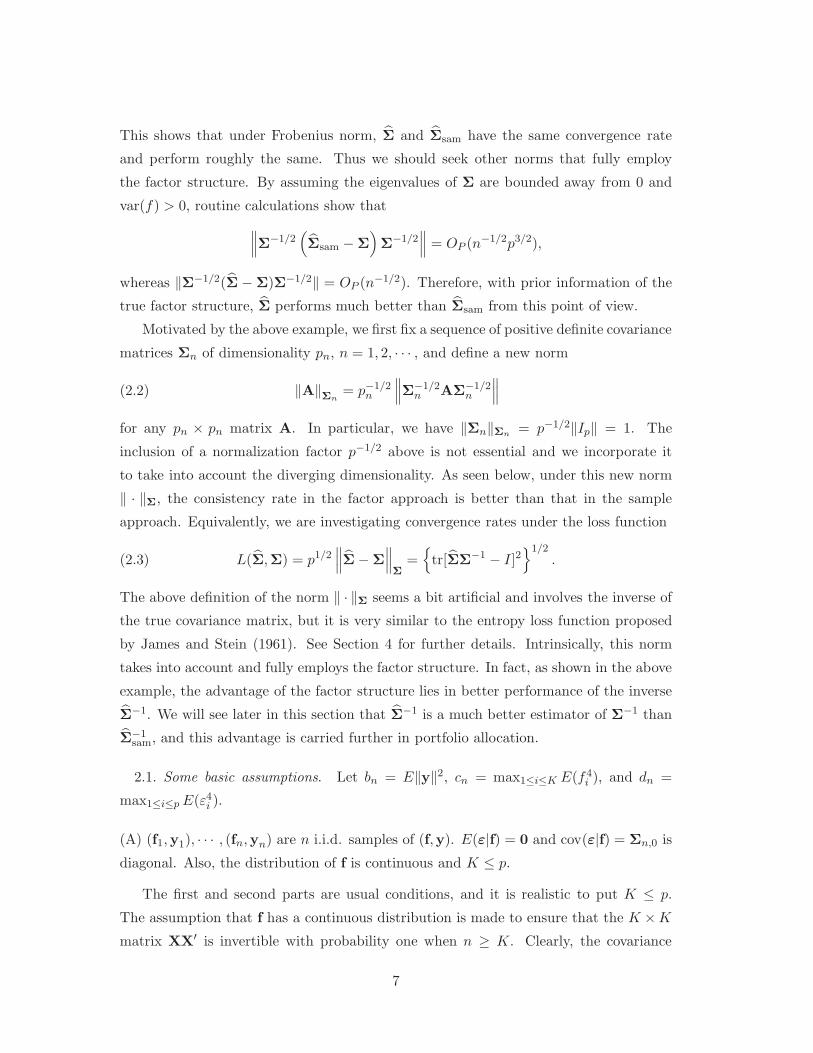
matrix estimation errors of Σ and Σsam under the Frobenius norm, the norm ‖ · ‖Σintroduced in Section 2, and the Stein (or entropy) loss function

L(Σ,Σ) = tr(ΣΣ−1

)− log

∣∣∣ΣΣ−1∣∣∣− p,

which was proposed by James and Stein (1961). Meanwhile, we compare estimation

errors of Σ−1 and Σ−1sam under the Frobenius norm. Furthermore, we evaluate estimated

variances of optimal portfolios with expected rate of return γn = 10% based on Σ

and Σsam by comparing their mean-squared errors (MSEs). For the estimated global

minimum variances, we also compare their MSEs. Moveover, we examine MSEs of

estimated variances of the equally weighted portfolio ξp = (1/p, · · · , 1/p), based on Σ

and Σsam, respectively.

For simplicity, we fix K = 3 in our simulation and consider the three-factor model

(4.1) Ypi = bpi1f1 + bpi2f2 + bpi3f3 + εi, i = 1, · · · , p.

Here, we use the first subscript p to stress that the three-factor model varies across

dimensionality p. As before, we let y = (Y1, · · · , Yp)′ and f = (f1, f2, f3)

′. The Fama-

French three-factor model [Fama and French (1993)] is a practical example of model

(4.1). To make our simulation more realistic, we take the parameters from a fit of the

Fama-French three-factor model.

In the Fama-French three-factor model, Yi is the excess return of the i-th stock or

portfolio, i = 1, · · · , p. The first factor f1 is the excess return of the proxy of the market

portfolio, which is the value-weighted return on all NYSE, AMEX and NASDAQ stocks

(from CRSP) minus the one-month Treasury bill rate (from Ibbotson Associates). The

other two factors are constructed using six value-weighted portfolios formed on size and

book-to-market. Specifically, the second factor f2, SMB (Small Minus Big),

SMB = 1/3 (Small Value + Small Neutral + Small Growth)

− 1/3 (Big Value + Big Neutral + Big Growth)

14

is the average return on the three small portfolios minus the average return on the three

big portfolios, and the third factor f3, HML (High Minus Low),

HML = 1/2 (Small Value + Big Value)

− 1/2 (Small Growth + Big Growth)

is the average return on the two value portfolios minus the average return on the two

growth portfolios. See their website http://mba.tuck.dartmouth.edu/pages/faculty

/ken.french/data_library.html for more details about their three factors and the

data sets of the three factors, risk free interest rates, and returns of many constructed

portfolios.

We first fit three-factor model (4.1) with n = 756 and p = 30 using the three-year

daily data of 30 Industry Portfolios from May 1, 2002 to Aug. 29, 2005, which are avail-

able at the above website. Then, as in (1.4), we get 30 estimated factor loading vectors

b1 = (b11, b12, b13), · · · , b30 = (b30,1, b30,2, b30,3) and 30 estimated standard deviations

σ1, · · · , σ30 of the errors, where bi and σi correspond to the i-th portfolio, i = 1, · · · , 30.The sample average of σ1, · · · , σ30 is 0.66081 with a sample standard deviation 0.3275.

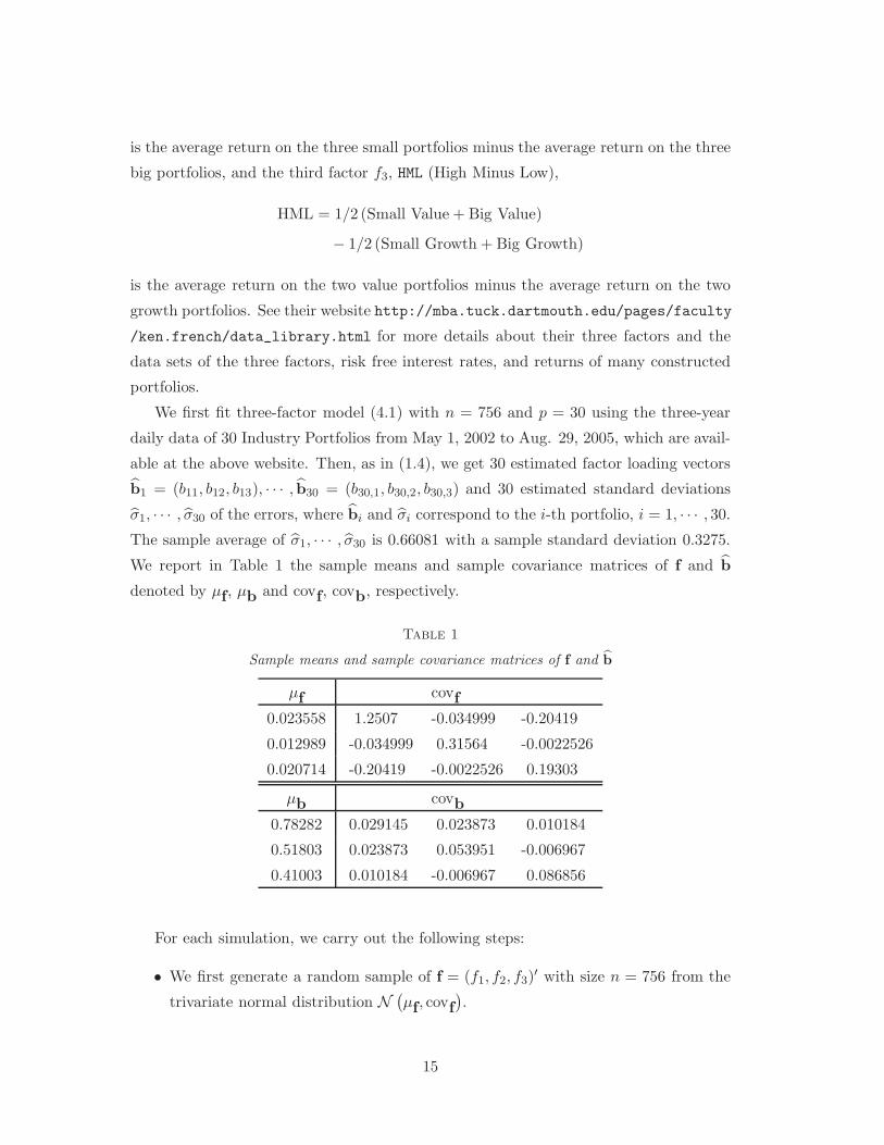
We report in Table 1 the sample means and sample covariance matrices of f and b

denoted by µf, µb and covf, covb, respectively.

Table 1

Sample means and sample covariance matrices of f and b

µf covf

0.023558 1.2507 -0.034999 -0.20419

0.012989 -0.034999 0.31564 -0.0022526

0.020714 -0.20419 -0.0022526 0.19303

µb covb

0.78282 0.029145 0.023873 0.010184

0.51803 0.023873 0.053951 -0.006967

0.41003 0.010184 -0.006967 0.086856

For each simulation, we carry out the following steps:

• We first generate a random sample of f = (f1, f2, f3)′ with size n = 756 from the

trivariate normal distribution N(µf, covf

).

15

• Then, for each dimensionality p increasing from 16 to 1000 with increment 20, we

do the following.

• Generate p factor loading vectors b1, · · · ,bp as a random sample of size p from

the trivariate normal distribution N(µb, covb

).

• Generate p standard deviations σ1, · · · , σp of the errors as a random sample of

size p from a gamma distribution G(α, β) conditional on being bounded below by

a threshold value. The threshold for the standard deviations of errors is required

in accordance with condition (C) in Section 2.1, and it is set to 0.1950 in our

simulation because we find min1≤i≤30 σi = 0.1950. Note that G(α, β) has mean

αβ and standard deviation α1/2β, and its conditional mean and conditional second

moment on falling above 0.1950 can be approximated respectively by

(αβ − 0.1950

2p

)/ (1 − p) and

(αβ2 + α2β2 − 0.19502

2p

)/ (1 − p) ,

where p is the probability of falling below 0.1950 under G(α, β). By matching the

mean 0.66081 and standard deviation 0.3275 for G(α0, β0), we obtain α0 = 4.0713

and β0 = 0.1623. Therefore, following the above approximations, by recursively

matching the conditional mean 0.66081 and conditional second moment 0.32752 +

0.660812 = 0.54393 for G(α, β), we finally get α = 3.3586 and β = 0.1876.

• After getting p standard deviations σ1, · · · , σp of the errors, we generate a random

sample of ε = (ε1, · · · , εp)′ with size n = 756 from the p-variate normal distribution

N(0,diag

(σ2

1, · · · , σ2p

)).

• Then from model (4.1), we get a random sample of y = (Y1, · · · , Yp)′ with size

n = 756.

• Finally, we compute estimated covariance matrices Σ and Σsam, as well as Σ−1

and Σ−1sam, and record the errors in the aforementioned measures. Meanwhile, we

calculate MSEs of estimated variances of the optimal portfolios with γn = 10%

as well as MSEs of estimated global minimum variances based on Σ and Σsam,

respectively. Also, we record MSEs of estimated variances of the equally weighted

portfolio based on Σ and Σsam, respectively.

We repeat the above simulation 500 times and report the mean-square errors as well as

the standard deviations of those errors.

16

0 200 400 600 800 10000

5

10

15

20

25

30

35

40

45

0 200 400 600 800 10000

0.2

0.4

0.6

0.8

1

1.2

1.4

(a) (b)

0 200 400 600 800 10000

0.2

0.4

0.6

0.8

1

1.2

1.4

0 200 400 600 800 10001

2

3

4

5

6

7

8

9

10x 10

−3

(c) (d)

0 50 100 150 200 250 300 350 400

0

20

40

60

80

100

120

140

0 50 100 150 200 250 300 350 4000

0.1

0.2

0.3

0.4

0.5

0.6

0.7

(e) (f)

Figure 1: (a), (c) and (e): The averages of errors over 500 simulations for bΣ (solid curve) and bΣsam (dashed

curve) against p under Frobenius norm, norm ‖ · ‖Σ and entropy losses, respectively. (b), (d) and (f): Corre-

sponding standard deviations of errors over 500 simulations for bΣ (solid curve) and bΣsam (dashed curve).

17

0 50 100 150 200 250 300 350 4000

50

100

150

200

250

300

0 50 100 150 200 250 300 350 4000

5

10

15

(a) (b)

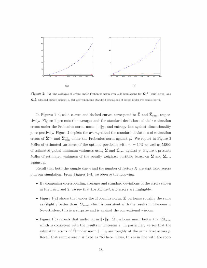
Figure 2: (a) The averages of errors under Frobenius norm over 500 simulations for bΣ−1 (solid curve) and

bΣ−1sam (dashed curve) against p. (b) Corresponding standard deviations of errors under Frobenius norm.

In Figures 1–4, solid curves and dashed curves correspond to Σ and Σsam, respec-

tively. Figure 1 presents the averages and the standard deviations of their estimation

errors under the Frobenius norm, norm ‖ · ‖Σ, and entropy loss against dimensionality

p, respectively. Figure 2 depicts the averages and the standard deviations of estimation

errors of Σ−1 and Σ−1sam under the Frobenius norm against p. We report in Figure 3

MSEs of estimated variances of the optimal portfolios with γn = 10% as well as MSEs

of estimated global minimum variances using Σ and Σsam against p. Figure 4 presents

MSEs of estimated variances of the equally weighted portfolio based on Σ and Σsam

against p.

Recall that both the sample size n and the number of factors K are kept fixed across

p in our simulation. From Figures 1–4, we observe the following:

• By comparing corresponding averages and standard deviations of the errors shown

in Figures 1 and 2, we see that the Monte-Carlo errors are negligible.

• Figure 1(a) shows that under the Frobenius norm, Σ performs roughly the same

as (slightly better than) Σsam, which is consistent with the results in Theorem 1.

Nevertheless, this is a surprise and is against the conventional wisdom.

• Figure 1(c) reveals that under norm ‖ · ‖Σ, Σ performs much better than Σsam,

which is consistent with the results in Theorem 2. In particular, we see that the

estimation errors of Σ under norm ‖ · ‖Σ are roughly at the same level across p.

Recall that sample size n is fixed as 756 here. Thus, this is in line with the root-

18

n-consistency of Σ under norm ‖ · ‖Σ when p = O(n) shown in Theorem 2. Also,

the apparent growth pattern of estimation errors in Σsam with p is in accordance

with its (n/p)1/2-consistency under norm ‖ · ‖Σ shown in Theorem 2.

• Figure 1(e) shows that under entropy loss, Σ significantly outperforms Σsam, which

strongly supports the factor-model based estimator Σ over the sample one Σsam.

We only report the results for p truncated at 400. This is because for larger

p, sample covariance matrices Σsam are nearly singular with a big chance in the

simulation, which results in extremely large entropy losses.

• From Figure 2(a), we see that under the Frobenius norm, the estimator Σ−1

significantly outperforms Σ−1sam, which is in line with the results in Theorem 3.

• Figures 3(a) and 3(b) demonstrate convincingly that Σ outperforms Σsam in port-

folio allocation. These results are in accordance with Theorems 5 and 6. One may

notice that in Figure 3(a), the MSEs are relatively large in magnitude for small

p and then tend to stabilize when p grows large. This is because in our settings

for the simulation, for small p the term ϕnφn − ψ2n is relatively small compared

to ϕnγ2n − 2ψnγn + φn, which results in large variance of the optimal portfolio.

The behavior of the MSEs for large p is essentially due to self-averaging in the

dimensionality. Figures 3(b) can be interpreted in the same way.

• Figure 4 reveals that the factor-model based approach and the sample approach

have almost the same performance in risk management, which is consistent with

Theorem 7. The high-dimensionality behavior is essentially due to self-averaging

as in Figure 3(a).

5. Concluding remarks. This paper investigates the impact of dimensionality on

the estimation of covariance matrices. Two estimators are singled out for studies and

comparisons: the sample covariance matrix and the factor-model based estimate. The

inverse of the covariance matrix takes advantage of the factor structure and hence can

be better estimated in the factor approach. As a result, when the parameters involve the

inverse of the population covariance, substantial gain can be made. On the other hand,

the covariance matrix itself does not take much advantage of the factor structure, and

hence its estimate can not be improved much in the factor approach. This is somewhat

surprising and is against the conventional wisdom.

19

0 200 400 600 800 10000

2

4

6

8

10

12

0 200 400 600 800 1000

0

1

2

3x 10

−4

(a) (b)

Figure 3: (a) The MSEs of estimated variances of the optimal portfolios with γn = 10% over 500 simulations

based on bΣ (solid curve) and bΣsam (dashed curve) against p. (b) The MSEs of estimated global minimum

variances over 500 simulations based on bΣ (solid curve) and bΣsam (dashed curve) against p.

0 200 400 600 800 10001

1.2

1.4

1.6

1.8

2

2.2

2.4

2.6x 10

−4

Figure 4: The MSEs of estimated variances of the equally weighted portfolio over 500 simulations based on bΣ

(solid curve) and bΣsam (dashed curve) against p.

20

Optimal portfolio allocation and minimum variance portfolio involve the inverse of

the covariance matrix. Hence, it is advantageous to employ the factor structure in

portfolio allocation. On the other hand, intrinsically the risk management does not

depend on the covariance structure and hence there is no advantage to appeal to the

factor model in risk management.

Our conclusion is also verified by an extensive simulation study, in which the param-

eters are taken in a neighborhood that is close to the reality. The choice of parameters

relies on a fit to the famous Fama-French three-factor model to the portfolios traded in

the market.

Our studies also reveal that the impact of dimensionality on the estimation of co-

variance matrices is severe. This should be taken into consideration in practical imple-

mentations.

6. Proofs of theorems. In this section, we give rigorous proofs of Theorems 1–7.

Proof of Theorem 1. (1) First, we prove (pK)−1 n1/2-consistency of Σ under

the Frobenius norm. To facilitate the presentation, we introduce here some notation

used throughout the rest of the paper. Let Cn = EX′(XX′)−1,

Dn ={(n− 1)−1

XX′ − [n(n− 1)]−1X11′X′

}− cov(f)

and

Fn = Ip ◦ n−1E (In − H)E′ − Σ0,

where H = X′ (XX′)−1

X is the n×n hat matrix and A1 ◦A2 stands for the Hadamard

product, i.e. the entrywise product, for any q × r matrices A1 and A2. Then we

have B = YX′ (XX′)−1

= B + Cn, cov(f) = (n− 1)−1XX′ − {n (n− 1)}−1

X11′X′ =

cov(f) + Dn, Σ0 = diag(n−1EE

′)

= Σ0 + Fn and

(6.1) Σ = Σ + BDnB′ +[Bcov(f)C′

n + Cncov(f)B′]+ Cncov(f)C′

n + Fn,

This shows that Σ is a four-term perturbation of the population covariance matrix,

and this representation is our key technical tool. By the Cauchy-Schwarz inequality, it

follows from (6.1) that

E‖Σ − Σ‖2 ≤ 4[E tr

{(BDnB

′)2}

+ E tr{[

Bcov(f)C′n + Cncov(f)B′

]2}

+ E tr{[

Cncov(f)C′n

]2}+ E tr

(F2

n

) ].

21

We will examine each of the above four terms on the right hand side separately. For

brevity of notation, we suppress the first subscript n in some situations where the

dependence on n is self-evident.

Before going further, let us bound ‖Bn‖. From assumption (B), we know that

cov(f) ≥ σ1IK , where for any symmetric positive semidefinite matrices A1 and A2,

A1 ≥ A2 means A1 −A2 is positive semidefinite. Thus it follows easily from (1.3) that

σ1BnB′n = Bn (σ1IK)B′

n ≤ Bncov(f)B′n ≤ Σn,

which along with bn = O(p) in assumption (B) shows that ‖Bn‖2 = tr (BnB′n) ≤

tr (Σn) /σ1 ≤ bn

σ1= O(p), i.e.

(6.2) ‖Bn‖ = O(p1/2).

Clearly, ‖B′nBn‖ = ‖BnB

′n‖, and by (A.1) in Lemma 1 and (6.2) we have

(6.3) ‖B′nBn‖ = ‖BnB

′n‖ ≤ ‖Bn‖‖B′

n‖ = ‖Bn‖2 = O(p).

This fact is a key observation that will be used very often, and as shown above, it is

entailed only by assumptions (A) and (B), which are valid throughout the paper.

Now we consider the first term, say E tr{(BDnB′)

2}. From cn = O(1) in assumption

(B), we see that the fourth moments of f are bounded across n, thus a routine calculation

reveals that

(6.4) E(‖Dn‖2

)= O(n−1K2),

which is an important fact that will be used very often and also helps study the inverse

cov(f)−1 by keeping in mind that K → ∞. By (A.2) in Lemma 1, (6.3), and (6.4), we

have

(6.5) E tr[(

BDnB′)2] ≤

∥∥B′B∥∥2E(‖Dn‖2

)= O(n−1(pK)2).

The remaining three terms are taken care of by Lemmas 2 and 3. Therefore, in view

of (6.3), combining (6.5) with (A.5)–(A.7) in Lemmas 2 and 3 gives

E∥∥∥Σ− Σ

∥∥∥2

= O(n−1(pK)2).

In particular, this implies that∥∥∥Σ − Σ

∥∥∥ = OP (n−1/2pK), which proves (pK)−1 n1/2-

consistency of the covariance matrix estimator Σ under Frobenius norm.

22

(2) Then, we show that Σsam is (pK)−1 n1/2-consistent under the Frobenius norm.

By (1.3) and (1.5), we have

Σsam = Σ + BDnB′ + Gn + (n− 1)−1 {

BXE′ + EX′B}

(6.6)

− [n (n− 1)]−1 {BX11′E′ + E11′X′B′

},

where Gn ={

(n− 1)−1EE′ − [n(n− 1)]−1

E11′E′}−Σ0. This shows that Σsam is also

a four-term perturbation of the population covariance matrix. By the Cauchy-Schwarz

inequality, it follows from (6.6) that

E∥∥∥Σsam − Σ

∥∥∥2≤ 4

[E∥∥BDnB

′∥∥2

+ E ‖Gn‖2 + 2 (n− 1)−2E∥∥BXE′

∥∥2

+ 2 [n (n− 1)]−2E∥∥BX11′E′

∥∥2].

As in part (1), we will examine each of the above four terms on the right hand side

separately. The first term E ‖BDnB′‖2

has been bounded in (6.5). Using the same

argument as in Lemma 6, we can show that E ‖Gn‖2 = O(n−1p2). In view of (6.3), it

is shown that

E∥∥BXE′

∥∥2= O(np2K)

in the proof of Lemma 2. Using the same argument as in Lemma 2 to boundE ‖BX11′HE′‖2,

we can easily get

E∥∥BX11′E′

∥∥2= O(n3p2K),

which along with (6.5) and the above results yields

E∥∥∥Σsam − Σ

∥∥∥2

= O(n−1(pK)2).

This proves (pK)−1 n1/2-consistency of Σsam under the Frobenius norm.

(3) Finally, we prove the uniform weak convergence of eigenvalues. It follows from

Corollary 6.3.8 of Horn and Johnson (1985) that

max1≤k≤p

∣∣∣λk(Σn) − λk(Σn)∣∣∣ ≤

{p∑

k=1

[λk(Σn) − λk(Σn)

]2}1/2

≤∥∥∥Σn − Σn

∥∥∥ .

Therefore, the uniform weak convergence of the eigenvalues of the Σn’s follows imme-

diately from the (pK)−1 n1/2-consistency of Σ under the Frobenius norm shown in part

(1). Similarly, by the (pK)−1 n1/2-consistency of Σsam under the Frobenius norm shown

in part (2), the same conclusion holds for Σsam. �

23

Proof of Theorem 2. (1) First, we show that Σ is nβ/2-consistent under norm

‖ · ‖Σ. The main idea of the proof is similar to that of Theorem 1, but the proof is more

tricky and involved here since the norm ‖ · ‖Σ involves the inverse of the covariance

matrix Σ. By the Cauchy-Schwarz inequality, it follows from (6.1) that

E∥∥∥Σ− Σ

∥∥∥2

Σ

≤ 4[E∥∥BDnB

′∥∥2

Σ+ E

∥∥Bcov(f)C′n + Cncov(f)B′

∥∥2

Σ

+ E∥∥Cncov(f)C′

n

∥∥2

Σ} + E ‖Fn‖2

Σ

].

As in the proof of Theorem 1, we will study each of the above four terms on the right

hand side separately.

Before going further, let us bound∥∥B′Σ−1B

∥∥. From (1.3), we know that Σ =

Σ0+Bcov(f)B′, which along with the Sherman-Morrison-Woodbury formula shows that

(6.7) Σ−1 = Σ−10 − Σ−1

0 B[cov(f)−1 + B′Σ−1

0 B]−1

B′Σ−10 .

Thus it follows that

B′Σ−1B = B′Σ−10 B− B′Σ−1

0 B[cov(f)−1 + B′Σ−1

0 B]−1

B′Σ−10 B

= B′Σ−10 B

[cov(f)−1 + B′Σ−1

0 B]−1

cov(f)−1

= cov(f)−1 − cov(f)−1[cov(f)−1 + B′Σ−1

0 B]−1

cov(f)−1,

which implies that

∥∥B′Σ−1B∥∥ ≤

∥∥cov(f)−1∥∥+

∥∥∥cov(f)−1[cov(f)−1 + B′Σ−1

0 B]−1

cov(f)−1∥∥∥ .

Note that cov(f)−1 is symmetric positive definite and B′Σ−10 B is symmetric positive

semidefinite. Thus, cov(f)−1+B′Σ−10 B ≥ cov(f)−1, which in turn implies that

[cov(f)−1 + B′Σ−1

0 B]−1 ≤

cov(f) and

cov(f)−1[cov(f)−1 + B′Σ−1

0 B]−1

cov(f)−1 ≤ cov(f)−1cov(f)cov(f)−1 = cov(f)−1.

In particular, this entails that

∥∥∥cov(f)−1[cov(f)−1 + B′Σ−1

0 B]−1

cov(f)−1∥∥∥ ≤

∥∥cov(f)−1∥∥ ,

so now the problem of bounding∥∥B′Σ−1B

∥∥ reduces to bounding∥∥cov(f)−1

∥∥. By as-

sumption (B), λK(cov(f)) ≥ σ1 for some constant σ1 > 0. Thus the largest eigenvalues

of cov(f)−1 are bounded across n, which easily implies that∥∥cov(f)−1

∥∥ = O(K1/2). This

together with the above results shows that

(6.8)∥∥B′Σ−1B

∥∥ = O(K1/2).

24

Now we are ready to examine the first term, say E ‖BDnB′‖2

Σ. By (A.1) in Lemma

1, we have

∥∥BDnB′∥∥2

Σ= p−1tr

[(DnB

′Σ−1B)2] ≤ p−1 ‖Dn‖2

∥∥B′Σ−1B∥∥2.

Therefore, it follows from (6.4) and (6.8) that

(6.9) E∥∥BDnB

′∥∥2

Σ= O(n−1p−1K3).

Then, we consider the second term E ‖Bcov(f)C′n + Cncov(f)B′‖2

Σ. Note that

E∥∥Bcov(f)C′

n + Cncov(f)B′∥∥2

Σ≤ 2

[E∥∥Bcov(f)C′

n

∥∥2

Σ+ E

∥∥Cncov(f)B′∥∥2

Σ

](6.10)

= 4 E∥∥Bcov(f)C′

n

∥∥2

Σ≤ 8[(n− 1)−2E

∥∥BXX′C′n

∥∥2

Σ

+ n−2 (n− 1)−2E∥∥BX11′X′C′

n

∥∥2

Σ

]

= 8 (n− 1)−2 L1 + 8n−2 (n− 1)−2 L2.

Since E(ε|f) = 0, conditioning on X gives

L1 = p−1E tr[XE

(E′Σ−1E|X

)X′B′Σ−1B

]

= p−1E tr[X tr

(Σ−1Σ0

)In X′B′Σ−1B

]

≤ p−1tr(Σ−1Σ0

)E(‖XX′‖

) ∥∥B′Σ−1B∥∥ .

In the proof of Lemma 2, it is shown that E(‖XX′‖2

)= O(n2K2), which implies that

E(‖XX′‖

)≤[E(‖XX′‖2

)]1/2= O(nK).

By (1.3) and assumptions (B) and (C), we can easily get

tr(Σ−1Σ0

)≤ tr

(Σ−1

)O(1) = O(p),

which along with (6.8) and the above results shows that

L1 = O(nK3/2).

Similarly, by conditioning on X we have

L2 = p−1E tr[X11′HE

(E′Σ−1E|X

)H11′X′B′Σ−1B

]

= p−1E tr[X11′H tr

(Σ−1Σ0

)In H11′X′B′Σ−1B

].

25

Then, applying (A.1)–(A.3) in Lemma 1 gives

L2 ≤ p−1tr(Σ−1Σ0

)E∥∥X11′H11′X′

∥∥∥∥B′Σ−1B∥∥

≤ p−1tr(Σ−1Σ0

)E ‖H‖

∥∥X′X∥∥ ∥∥11′11′

∥∥ ∥∥B′Σ−1B∥∥

= n2p−1K1/2tr(Σ−1Σ0

)E∥∥X′X

∥∥ ∥∥B′Σ−1B∥∥ ,

which together with the above results shows that

L2 = O(n3K2).

Thus, in view of (6.10) we have

(6.11) E∥∥Bcov(f)C′

n + Cncov(f)B′∥∥2

Σ= O(n−1K2).

The third and fourth terms are examined in Lemmas 4 and 5, respectively. Since

K ≤ p by assumption (A), combining (6.9) and (6.11) with (A.8) and (A.11) in Lemmas

4 and 5 results in

E∥∥∥Σ − Σ

∥∥∥2

Σ

= O(n−1K2) +O(n−2pK).

In particular, when K = O(nα1) and p = O(nα) for some 0 ≤ α1 < 1/2 and 0 ≤ α <

2 − α1, we have ∥∥∥Σ − Σ

∥∥∥Σ

= OP (n−β/2)

with β = min (1 − 2α1, 2 − α− α1), which proves nβ/2-consistency of covariance matrix

estimator Σ under norm ‖ · ‖Σ.

(2) Then, we prove the nβ1/2-consistency of Σsam under norm ‖·‖Σ. By the Cauchy-

Schwarz inequality, it follows from (6.6) that

E∥∥∥Σsam − Σ

∥∥∥2

Σ

≤ 4[E∥∥BDnB

′∥∥2

Σ+ E ‖Gn‖2

Σ+ 2 (n− 1)−2E

∥∥BXE′∥∥2

Σ

+ 2 [n (n− 1)]−2E∥∥BX11′E′

∥∥2

Σ

].

As in part (1), we will examine each of the above four terms on the right hand side

separately. The first term E ‖BDnB′‖2

Σhas been bounded in (6.9), and the second

term E ‖Gn‖2Σ

is considered in Lemma 6. The third term E ‖BXE′‖2Σ

is exactly L1 in

part (1) above. Using the same argument that was used in part (1) to prove L2, we can

easily get

E∥∥BX11′E′

∥∥2

Σ= O(n3K3/2).

Thus, by (6.9) and (A.12) in Lemma 6 along with the above results, we have

E∥∥∥Σsam − Σ

∥∥∥2

Σ

= O(n−1p−1K3) +O(n−1p) +O(n−1K3/2).

26

In particular, when K = O(nα1) and p = O(nα) for some 0 ≤ α < 1 and 0 ≤ α1 <

(1 + α) /3, we have ∥∥∥Σsam − Σ

∥∥∥Σ

= OP (n−β1/2)

with β1 = 1 − max(α, 3α1/2, 3α1 − α), which shows nβ1/2-consistency of Σsam under

norm ‖ · ‖Σ. �

Proof of Theorem 3. (1) First, we prove the weak convergence of Σ−1sam under

the Frobenius norm. Note that Σsam involves sample covariance matrix estimation of

Σ0, so the technique in part (2) below does not help. In general, the only available way

is as follows. We define Qn = Σsam −Σn. It is a basic fact in matrix theory that

(6.12)∥∥∥Σ−1

sam − Σ−1n

∥∥∥ ≤∥∥Σ−1

n

∥∥∥∥Σ−1

n Qn

∥∥1 −

∥∥Σ−1n Qn

∥∥ ≤∥∥Σ−1

n

∥∥2 ‖Qn‖1 −

∥∥Σ−1n

∥∥ ‖Qn‖

whenever∥∥Σ−1

n

∥∥ ‖Qn‖ < 1. From Theorem 1, we know that

‖Qn‖ = OP (n−1/2pK).

By (A.9), we have∥∥Σ−1

n

∥∥ = O(p1/2). Since pK1/2 = o((n/ log n)1/4) we see that

∥∥Σ−1n

∥∥ ‖Qn‖P−→ 0 and

√np−4K−2/ log n

∥∥Σ−1n

∥∥2 ‖Qn‖P−→ 0.

It follows easily that

√np−4K−2/ log n

∥∥Σ−1n

∥∥2 ‖Qn‖1 −

∥∥Σ−1n

∥∥ ‖Qn‖P−→ 0,

which along with (6.12) shows that

√np−4K−2/ log n

∥∥∥Σ−1sam − Σ−1

n

∥∥∥ P−→ 0 as n→ ∞.

(2) Then, we show the weak convergence of Σ−1 under the Frobenius norm. The

basic idea is to examine the estimation error for each term of Σ−1, which has an explicit

form thanks to the factor structure. From (1.4), we know that Σ = Bcov(f)B′+ Σ0,

which along with the Sherman-Morrison-Woodbury formula shows that

(6.13) Σ−1 = Σ−10 − Σ−1

0 B[cov(f)−1 + B

′Σ−1

0 B]−1

B′Σ−1

0 .

27

Thus by (6.7), we have

∥∥∥Σ−1 −Σ−1∥∥∥ ≤

∥∥∥Σ−10 −Σ−1

0

∥∥∥+

∥∥∥∥(Σ−1

0 − Σ−10

)B[cov(f)−1 + B

′Σ−1

0 B]−1

B′Σ−1

0

∥∥∥∥

(6.14)

+

∥∥∥∥Σ−10 B

[cov(f)−1 + B

′Σ−1

0 B]−1

B′(Σ−1

0 − Σ−10

)∥∥∥∥

+

∥∥∥∥Σ−10

(B− B

) [cov(f)−1 + B

′Σ−1

0 B]−1

B′Σ−1

0

∥∥∥∥

+

∥∥∥∥Σ−10 B

[cov(f)−1 + B

′Σ−1

0 B]−1 (

B′ − B′

)Σ−1

0

∥∥∥∥

+

∥∥∥∥Σ−10 B

{[cov(f)−1 + B

′Σ−1

0 B]−1

−[cov(f)−1 + B′Σ−1

0 B]−1}

B′Σ−10

∥∥∥∥

= K1 + K2 + K3 + K4 + K5 + K6.

To study∥∥∥Σ−1 − Σ−1

∥∥∥, we need to examine each of the above six terms K1, · · · ,K6

separately, so it would be lengthy work to check all the details here. Therefore, we only

sketch the idea of the proof and leave the details to the reader.

From assumption (C), we know that the diagonal entries of Σ0 are bounded away

from 0. Note that Σ0 and Σ0 are both diagonal, and thus, by the same argument as in

Lemma 5, we can easily show that

(6.15) K1 =∥∥∥Σ−1

0 − Σ−10

∥∥∥ = OP (n−1/2p1/2) +OP (n−1pK1/2) = OP (n−1/2p1/2),

since pK1/2 = o((n/ log n)1/2). Now we consider the second term K2. By (A.1) in

Lemma 1, we have

K2 ≤∥∥∥(Σ−1

0 − Σ−10

)Σ

1/20

∥∥∥∥∥∥∥Σ

−1/20 B

[cov(f)−1 + B

′Σ−1

0 B]−1

B′Σ

−1/20

∥∥∥∥∥∥∥Σ−1/2

0

∥∥∥

= L1L2

∥∥∥Σ−1/20

∥∥∥ ,

and we will examine each of the above two terms L1 and L2, as well as∥∥∥Σ−1/2

0

∥∥∥. Since

Σ0 and Σ0 are diagonal, a similar argument to that bounding K1 above applies to show

that ∥∥∥Σ−1/20

∥∥∥ = OP (p1/2) and L1 = OP (n−1/2p1/2).

Clearly, Σ−1/20 B

[cov(f)−1 + B

′Σ−1

0 B]−1

B′Σ

−1/20 is symmetric positive semidefinite with

rank at most K and Σ1/20 Σ−1Σ

1/20 ≥ 0. Thus it follows from (6.13) that

Σ−1/20 B

[cov(f)−1 + B

′Σ−1

0 B]−1

B′Σ

−1/20 = Ip − Σ

1/20 Σ−1Σ

1/20 ≤ Ip,

28

which implies that Σ−1/20 B

[cov(f)−1 + B

′Σ−1

0 B]−1

B′Σ

−1/20 has at most K positive

eigenvalues and all of them are bounded by one. This shows that L2 ≤ K1/2, which

along with the above results gives

(6.16) K2 = OP (n−1/2pK1/2).

Similarly, we can also show that

(6.17) K3 = OP (n−1/2pK1/2).

Then we consider terms K4 and K5. Clearly, cov(f)−1 + B′Σ−1

0 B ≥ cov(f)−1, which

in turn entails that[cov(f)−1 + B

′Σ−1

0 B]−1

≤ cov(f) and

∥∥∥∥[cov(f)−1 + B

′Σ−1

0 B]−1∥∥∥∥ ≤ ‖cov(f)‖ .

It is easy to show that ‖cov(f)‖ = OP (K). Thus we have

K4 ≤∥∥∥Σ−1

0

(B− B

)∥∥∥∥∥∥∥[cov(f)−1 + B

′Σ−1

0 B]−1∥∥∥∥∥∥∥B′

Σ−10

∥∥∥(6.18)

= OP (n−1p1/2)OP (K)OP (p1/2) = OP (n−1/2pK)

and

K5 ≤∥∥Σ−1

0 B∥∥∥∥∥∥[cov(f)−1 + B

′Σ−1

0 B]−1∥∥∥∥∥∥∥(B

′ − B′)Σ−1

0

∥∥∥(6.19)

= OP (p1/2)OP (K)OP (n−1p1/2K) = OP (n−1/2pK).

Finally, by the same argument as in part (1) above, we can show that

∥∥∥∥[cov(f)−1 + B

′Σ−1

0 B]−1

−[cov(f)−1 + B′Σ−1

0 B]−1∥∥∥∥ = oP ((n/ log n)−1/2K2).

Thus by (A.2) in Lemma 1, we have

K6 ≤∥∥∥∥[cov(f)−1 + B

′Σ−1

0 B]−1

−[cov(f)−1 + B′Σ−1

0 B]−1∥∥∥∥∥∥B′Σ−2

0 B∥∥(6.20)

= oP ((n/ log n)−1/2K2)O(p) = oP ((n/ log n)−1/2 pK2).

Therefore, it follows from (6.14)–(6.20) that

√np−2K−4/ log n

∥∥∥Σ−1n − Σ−1

n

∥∥∥ P−→ 0 as n→ ∞,

which completes the proof. �

29

Proof of Theorem 4. We aim at establishing asymptotic normality of the K×Kmatrix

√np−2B′

(Σ − Σ

)B, and only here are the K factors f1, · · · , fK assumed fixed

across n. The basic idea is to use its four-term decomposition below and to show that

the first term has asymptotic normality by the classical central limit theorem, while the

remaining three terms are all negligible, say oP (1), which along with Slutsky’s theorem

leads to the desired conclusion. In view of (6.1), we have

√np−2B′

(Σ − Σ

)B =

√np−2B′BDnB

′B +√np−2B′

{Bcov(f)C′

n + Cncov(f)B′}B

+√np−2B′Cncov(f)C′

nB +√np−2B′FnB

= A1 + A2 + A3 + A4.(6.21)

We will study each of the above four terms A1, · · · ,A4 separately.

First, we consider the term A1. Define

Hn =n

n− 1

(n−1

n∑

i=1

fi − Ef

)(n−1

n∑

i=1

f′i − Ef′

).

Then we have

(6.22) cov(f) = (n− 1)−1n∑

i=1

(fi − Ef)(f′i − Ef′

)−Hn.

By the classical central limit theorem, we know that

√n

(n−1

n∑

i=1

fi − Ef

)D−→ N (0, cov(f)) .

It follows from the law of large numbers that n−1∑n

i=1 fi−EfP−→ 0. Thus, by Slutsky’s

theorem we have√nHn

D−→ 0, which in turn implies that

√nHn

P−→ 0;

that is, Hn = oP (n−1/2). So in view of (6.22), we have

(6.23) cov(f) = n−1n∑

i=1

(fi − Ef)(f′i − Ef′

)+ oP (n−1/2).

Therefore, it follows easily from p−1B′nBn → A and (6.23) that

(6.24) A1 = A

{n−1/2

n∑

i=1

[(fi −Ef)

(f′i − Ef′

)− cov(f)

]}

A + oP (1).

30

We define

n−1/2n∑

i=1

[(fi − Ef)

(f′i − Ef′

)− cov(f)

]= Un = (uij)K×K .

By the classical central limit theorem, we know that [see, e.g. Muirhead (1982)]

(6.25) vech (Un)D−→ N (0,H) ,

where H is determined in an obvious way by

cov (uij, ukl) = κijkl + κikκjl + κilκjk,

with κi1···ir the central moment E [(fi1 −Efi1) · · · (fir − Efir)] of f = (f1, · · · , fK)′. It

follows easily from (6.24) and (6.25) that

(6.26) vech (A1)D−→ N (0, G) ,

where G = PD (A⊗ A)DHD′ (A⊗ A)P ′D, D is the duplication matrix of order K, and

PD = (D′D)−1D′.

Then, we examine the second term A2. From p−1B′nBn → A, we know that

(6.27)∥∥B′

nBn

∥∥ =∥∥BnB

′n

∥∥ = O(p),

which is in line with (6.3). It follows that

‖A2‖ ≤ 2∥∥√np−2B′Bcov(f)C′

nB∥∥ ≤ 2n1/2p−2

∥∥B′B∥∥ ∥∥cov(f)C′

nB∥∥(6.28)

≤ 2n1/2p−2∥∥B′B

∥∥{

(n− 1)−1∥∥XE′B

∥∥+ n−1 (n− 1)−1∥∥X11′HE′B

∥∥}

= O(n−1/2p−1)∥∥XE′B

∥∥+O(n−3/2p−1)∥∥X11′HE′B

∥∥ .

Since E(ε|f) = 0 and Σ0 is diagonal, conditioning on X gives

E∥∥XE′B

∥∥2= E tr

[XE

(E′BB′E|X

)X′]

= E tr[X tr

(BB′Σ0

)In X′

]

= tr(BB′Σ0

)E ‖X‖2 = O(p)O(n) = O(np).

Similarly, by conditioning on X we have

E∥∥X11′HE′B

∥∥2= E tr

[X11′HE

(E′BB′E′|X

)H11′X′

]

= E tr[X11′H tr

(BB′Σ0

)In H11′X′

]

31

and then applying (A.2) and (A.3) in Lemma 1 yields

E∥∥X11′Hε′B

∥∥2 ≤ tr(BB′Σ0

)E{∥∥X′X

∥∥ ∥∥11′11′∥∥ ‖H‖

}

≤ O(p)n2K1/2{E(‖X′X‖2

)}1/2= O(n3p).

It follows that ‖XE′B‖ = OP (n1/2p1/2) and ‖X11′HE′B‖ = OP (n3/2p1/2), which to-

gether with (6.28) shows that

(6.29) A2 = oP (1);

that is, A2 is a negligible term.

Finally, the third and fourth terms A3 and A4 can also be shown to be negligible by

invoking Lemma 3. By (6.27) and (A.6) and (A.7) in Lemma 3, we have

E∥∥B′Cncov(f)C′

nB∥∥2 ≤

∥∥BB′∥∥2E∥∥Cncov(f)C′

n

∥∥2

= O(p2)O(n−2p2) = O(n−2p4)

and

E∥∥B′FnB

∥∥2 ≤∥∥BB′

∥∥2E ‖Fn‖2 = O(p2)O(n−1p) = O(n−1p3).

It follows that ‖B′Cncov(f)C′nB‖ = OP (n−1p2) and ‖B′FnB‖ = OP (n−1/2p3/2), which

implies that

(6.30) A3 = oP (1) and A4 = oP (1).

Therefore, in view of (6.26), (6.29), and (6.30), applying Slutsky’s theorem gives

√n vech

[p−2B′

n

(Σn − Σn

)Bn

]D−→ N (0, G) ,

which proves the asymptotic normality of covariance matrix estimator Σ. �

Proof of Theorem 5. (1) First, we prove the weak convergence of the estimated

global minimum variance based on Σ. From Theorem 3, we know that

√np−2K−4/ log n

∥∥∥Σ−1 −Σ−1∥∥∥ P−→ 0.

Note that

|ϕn − ϕn| =∣∣∣1′(Σ−1 − Σ−1

)1

∣∣∣ =∣∣∣tr[(

Σ−1 − Σ−1)11′]∣∣∣

≤∥∥∥Σ−1 −Σ−1

∥∥∥∥∥11′

∥∥ = p∥∥∥Σ−1 − Σ−1

∥∥∥ .

32

Thus we have √n (pK)−4 / log n |ϕn − ϕn| P−→ 0.

Since all the ϕn’s are bounded away from zero, it follows easily that√n (pK)−4 / log n

∣∣∣ξ′ngΣnξng − ξ′ngΣnξng

∣∣∣ =

√n (pK)−4 / log n

∣∣ϕ−1n − ϕ−1

n

∣∣ P−→ 0.

(2) Then, we prove the conclusion for Σsam. From Theorem 3, we know that

√np−4K−2/ log n

∥∥∥Σ−1sam − Σ−1

∥∥∥ P−→ 0.

Therefore, the above argument in part (1) applies to show that

√np−6K−2/ log n

∣∣∣ξ′ngΣsamξng − ξ′ngΣnξng

∣∣∣ =√np−6K−2/ log n

∣∣ϕ−1n − ϕ−1

n

∣∣ P−→ 0. �

Proof of Theorem 6. (1) First, we prove the weak convergence of the estimated

variance of the optimal portfolio based on Σ. From Theorem 3, we know that

(6.31)√np−2K−4/ log n

∥∥∥Σ−1 −Σ−1∥∥∥ P−→ 0,

and from part (1) in the proof of Theorem 5, we see that

(6.32)

√n (pK)−4 / log n |ϕn − ϕn| P−→ 0.

Now we show the same rate for∣∣∣ψn − ψn

∣∣∣, say

(6.33)

√n (pK)−4 / log n

∣∣∣ψn − ψn

∣∣∣ P−→ 0.

By bn = O(p) in assumption (B), a routine calculation yields ‖µn‖ = O(p1/2) and

E ‖µn − µn‖2 = O(n−1p), and thus

‖µn − µn‖ = OP (n−1/2p1/2).

It follows that∣∣∣ψn − ψn

∣∣∣ ≤∣∣∣1′(Σ−1 − Σ−1

)µ

∣∣∣+∣∣1′Σ−1 (µ − µ)

∣∣ ≤∥∥1′∥∥∥∥∥Σ−1 −Σ−1

∥∥∥

· (‖µ‖ + ‖µ − µ‖) +∥∥1′∥∥ ∥∥Σ−1

∥∥ ‖µ − µ‖ .

Then we have∣∣∣ψn − ψn

∣∣∣ ≤ p1/2∥∥∥Σ−1 − Σ−1

∥∥∥[O(p1/2) +OP (n−1/2p1/2)

]

+ p1/2O(p1/2)OP (n−1/2p1/2)

=∥∥∥Σ−1 − Σ−1

∥∥∥O(p) +OP (n−1/2p3/2) =∥∥∥Σ−1 − Σ−1

∥∥∥O(p),

33

which together with (6.31) proves (6.32). Similarly, we can also show that

(6.34)

√n (pK)−4 / log n

∣∣∣φn − φn

∣∣∣ P−→ 0.

Since ϕnφn − ψ2n are bounded away from zero and ϕn/(ϕnφn − ψ2

n), ψn/(ϕnφn − ψ2n),

φn/(ϕnφn − ψ2n), γn are bounded, the conclusion follows from (3.3) and (6.32)–(6.34).

(2) Now we prove the conclusion for Σsam. From Theorem 3, we know that

√np−4K−2/ log n

∥∥∥Σ−1sam − Σ−1

∥∥∥ P−→ 0,

and from part (2) in the proof of Theorem 5, we see that

√np−6K−2/ log n |ϕn − ϕn| P−→ 0.

Since bn = O(p) by assumption (B), a routine calculation shows that

‖µsam − µn‖ = OP (n−1/2p1/2),

where µsam is the sample mean of µn. Therefore, the argument in part (1) above applies

to show that

√np−6K−2/ log n

∣∣∣ξ′nΣsamξn − ξ′nΣnξn

∣∣∣ P−→ 0 as n→ ∞. �

Proof of Theorem 7. Since ξn = O(1)1, the conclusion follows easily from

consistency results of Σ and Σsam under the Frobenius norm in Theorem 1. In particular,

when the portfolios ξn = (ξ1, · · · , ξp)′ have no short positions, we have

‖ξn‖ =√ξ21 + · · · + ξ2p ≤

√ξ1 + · · · + ξp = 1.

It therefore follows easily that√n (pK)−2 / log n

∣∣∣ξ′nΣnξn − ξ′nΣnξn

∣∣∣ P−→ 0 as n→ ∞

and √n (pK)−2 / log n

∣∣∣ξ′nΣsamξn − ξ′nΣnξn

∣∣∣ P−→ 0 as n→ ∞. �

APPENDIX

Throughout the paper, we denote by H the n× n hat matrix X′ (XX′)−1

X, which

is symmetric and positive semidefinite with probability one by assumption (A).

Lemma 1 (Basic facts).

34

(i) For any q × r matrix A1 and r × q matrix A2, we have

(A.1) |tr (A1A2)| ≤ ‖A1‖ ‖A2‖ and ‖A1A2‖ ≤ ‖A1‖ ‖A2‖ .

In particular, for any q × r matrix A1 and r × r symmetric matrix A2, we have

(A.2)∣∣tr(A1A2A

′1

)∣∣ ≤∥∥A′

1A1

∥∥ ‖A2‖ and∥∥A1A2A

′1

∥∥ ≤∥∥A′

1A1

∥∥ ‖A2‖ .

(ii) With probability one, the hat matrix H is idempotent with

(A.3) tr(H2)

= tr (H) = K,

and it satisfies

(A.4) 0 ≤ tr(H11′H

)≤ K1/2n and 0 ≤ tr

[(H11′H

)2] ≤ Kn2.

Proof. One can refer to Horn and Johnson (1990) for standard proofs of (A.1) and

(A.2). The fact that the hat matrix H is idempotent with (A.3) is known in multivariate

statistical analysis. Clearly, tr (H11′H) = 1′H1 ≥ 0. Thus by (A.1) and (A.3), we have

tr(H11′H

)= tr

(H11′

)≤ ‖H‖

∥∥11′∥∥ = K1/2n

and

tr[(

H11′H)2]

= tr[(

H11′)2] ≤

∥∥H11′∥∥2 ≤ ‖H‖2

∥∥11′∥∥2

= Kn2.

This completes the proof. �

The main trick in the proofs of the technical lemmas below is conditioning on X and

resorting to the basic facts from Lemma 1.

Lemma 2. Under conditions (A) and (B), we have

(A.5) E tr{[

Bcov(f)C′n + Cncov(f)B′

]2} ≤∥∥B′B

∥∥O(n−1pK3/2).

Proof. It follows from (A.1) that

E tr{[

Bcov(f)C′n + Cncov(f)B′

]2} ≤ 2 (n− 1)−2E tr{[

BXE′ + EX′B′]2}

+ 2n−2 (n− 1)−2E tr{[

BX11′HE′ + EH11′X′B′]2}

= 2 (n− 1)−2 A1 + 2n−2 (n− 1)−2 A2.

We will consider the above two terms A1 and A2 separately. By cn = O(1) in assumption

(B), we can easily get∥∥E(ff′)∥∥ = O(K) and E

(‖f‖4

)= O(K2).

35

Since E(E|f) = 0, by (A.1) and (A.2) conditioning on X results in

E∥∥BXE′

∥∥2= E tr

[BXE

(E′E|X

)X′B′

]= E tr

[BX tr (Σ0) In X′B′

]

= n tr (Σ0)E tr[Bff′B′

]= n tr (Σ0) tr

[BE

(ff′)B′]

≤ n tr (Σ0)∥∥B′B

∥∥∥∥E(ff′)∥∥ =

∥∥B′B∥∥ tr (Σ0)O(nK).

Similarly, by conditioning on X we have

E∥∥BX11′HE′

∥∥2= E tr

[BX11′HE

(E′E|X

)H11′X′B′

]

= E tr[BX11′H tr (Σ0) In H11′X′B′

],

and then applying (A.1) and (A.2) in Lemma 1 gives

E∥∥BX11′HE′

∥∥2 ≤ tr (Σ0) E{∥∥B′B

∥∥∥∥X′X∥∥ ∥∥11′11′

∥∥ ‖H‖}

≤ K1/2n2∥∥B′B

∥∥ tr (Σ0){E(∥∥X′X

∥∥2)}1/2

.

Note that E(‖X′X‖2

)= nE

(‖f‖4

)+ n (n− 1)

∥∥E(ff′)∥∥2

= O(n2K2). Thus,

E∥∥BX11′HE′

∥∥2 ≤∥∥B′B

∥∥ tr (Σ0)O(n3K3/2).

Therefore, by (A.1) we have

A1 ≤ 4E∥∥BXE′

∥∥2 ≤∥∥B′B

∥∥ tr (Σ0)O(nK)

and

A2 ≤ 4E∥∥BX11′HE′

∥∥2 ≤∥∥B′B

∥∥ tr (Σ0)O(n3K3/2),

which together yield (A.5) since clearly tr (Σ0) = O(p). �

Lemma 3. Under conditions (A) and (B), we have

(A.6) E tr{[

Cncov(f)C′n

]2}= O(n−2p2K)

and

(A.7) E tr(F2

n

)= O(n−1pK) +O(n−2p2K).

Proof. The proofs of (A.6) and (A.7) are similar to those in Lemmas 4 and 5

below, respectively. For brevity, we omit them here. �

Lemma 4. Under conditions (A)–(C), we have

(A.8) E∥∥Cncov(f)C′

n

∥∥2

Σ= O(n−2pK).

36

Proof. Note that

E∥∥Cncov(f)C′

n

∥∥2

Σ≤ 2 (n− 1)−2E

∥∥EHE′∥∥2

Σ+ 2n−2 (n− 1)−2E

∥∥EH11′HE′∥∥2

Σ

= 2 (n− 1)−2 K1 + 2n−2 (n− 1)−2 K2.

We will consider the above two terms K1 and K2 separately. First, we study the term

K1, which can further be decomposed into four terms. Since E (ε|f) = 0, by conditioning

on X we have

K1 = p−1E tr

E

n∑

i,j=1

Hijεiε′jΣ

−1n∑

k,l=1

Hklεkε′lΣ

−1|X

= p−1L1 + p−1L2 + p−1L3 + p−1L4,

where

L1 = E tr

{n∑

i=1

(Hii)2E[(

εiε′iΣ

−1)2]}, L2 = E tr

∑

i6=j

HiiHjjE(εiε

′iΣ

−1εjε′jΣ

−1) ,

L3 = E tr

∑

i6=j

(Hij)2E[(

εiε′jΣ

−1)2] , L4 = E tr

∑

i6=j

HijHjiE(εiε

′jΣ

−1εjε′iΣ

−1) ,

and Hij is the (i, j)-entry of the n × n hat matrix H. Then we consider each of these

four terms separately. By (1.3) and assumptions (C) and (B), it is easy to see that

(A.9) tr(Σ−1

)= O(p),

∥∥Σ−1∥∥ = O(p1/2), and tr

[(Σ0Σ

−1)2]

= O(p).

It follows from (A.3) and (A.9) that

L1 ≤ K E{

tr[(

εε′Σ−1)2]}

= K E

p∑

i,j=1

(Σ−1

)ijεiεj

p∑

k,l=1

(Σ−1

)klεkεl

= K

p∑

i=1

(Σ−1

)2iiE(ε4i)

+K∑

i6=j

(Σ−1

)ii

(Σ−1

)jjE(ε2i)E(ε2j)

+ 2K∑

i6=j

E(ε2i) (

Σ−1)ijE(ε2j) (

Σ−1)ji

≤[tr(Σ−1

)]2O(K) + tr

(Σ0Σ

−1Σ0Σ−1)O(K) = O(p2K)

and

L2 = E

∑

i6=j

HiiHjj tr[E(εε′)Σ−1E

(εε′)Σ−1

]

≤ tr[(

Σ0Σ−1)2]

E{[tr (H)]2

}= O(pK2).

37

Similarly, we have

L3 ≤ K tr{E[(

εη′Σ−1)2]}

= K E

p∑

i,j=1

(Σ−1)ij ηiεj

p∑

k,l=1

(Σ−1)kl ηkεl

= K

p∑

i=1

(Σ−1

)2iiE(η2

i

)E(ε2i)

+ 2K∑

i6=j

E(η2

i

) (Σ−1

)ijE(ε2j) (

Σ−1)ji

≤∥∥Σ−1

∥∥2O(K) + tr

(Σ0Σ

−1Σ0Σ−1)O(K) = O(pK)

and

L4 ≤ K tr[E(εη′Σ−1ηε′Σ−1

)]= K

[E(ε′Σ−1ε

)]2= K

[p∑

i=1

(Σ−1)iiE(ε2i )

]2

= K[tr(Σ−1

)O(1)

]2= O(p2K),

where η = (η1, · · · , ηp)′ is an independent copy of ε = (ε1, · · · , εp)′. Since K ≤ p by

assumption (A), combining L1, L2, L3, and L4 together gives

(A.10) K1 = E∥∥EHE′

∥∥2

Σ= O(pK).

Now we consider the second term K2. By (A.4), the same calculation as above

applies to show that

K2 = E∥∥EH11′HE′

∥∥2

Σ= O(n2pK).

Therefore, combining the above results together yields (A.8). �

Lemma 5. Under conditions (A)–(C), we have

(A.11) E‖Fn‖2Σ

= O(n−1) +O(n−2pK).

Proof. Note that

E‖Fn‖2Σ≤ 2E

∥∥Ip ◦ n−1EE′ − Σ0

∥∥2

Σ+ 2n−2E

∥∥Ip ◦ EHE′∥∥2

Σ.

Since E (ε) = 0 and cov (ε|f) = Σ0, we have

E∥∥Ip◦n−1EE′ − Σ0

∥∥2

Σ= p−1E

∥∥∥n−1Σ−1/2(Ip ◦EE′

)Σ−1/2 − Σ−1/2Σ0Σ

−1/2∥∥∥

2

Σ

= p−1n−1

[E∥∥∥Σ−1/2diag

(ε21, · · · , ε2p

)Σ−1/2

∥∥∥2−∥∥∥Σ−1/2Σ0Σ

−1/2∥∥∥

2]

≤ p−1n−1E tr

{[Σ−1/2diag

(ε21, · · · , ε2p

)Σ−1/2

]2}= p−1n−1L.

38

It follows from (A.9) that

L =

p∑

i,j=1

E[ε2i(Σ−1

)ijε2j(Σ−1

)ji

]=

p∑

i=1

(Σ−1

)2iiE(ε4)

+∑

i6=j

(Σ−1

)2ij

[E(ε2)]2

=∥∥Σ−1

∥∥2O(1) = O(p),

which shows that E∥∥Ip ◦ n−1EE′ − Σ0

∥∥2

Σ= O(n−1). The argument proving (A.10) in

Lemma 4 applies to show that

E∥∥Ip ◦ EHE′

∥∥2

Σ= O(pK).

Hence, combining the above results together gives (A.11). �

Lemma 6. Under conditions (A)–(C), we have

(A.12) E‖Gn‖2Σ

= O(n−1p).

Proof. Recall that Gn ={(n− 1)−1

EE′ − [n(n− 1)]−1E11′E′

}−Σ0, as defined

in part (2) of the proof of Theorem 1. Note that

E‖Gn‖2Σ≤ 3E

∥∥n−1EE′ −Σ0

∥∥2

Σ+ 3n−2 (n− 1)−2E

∥∥EE′∥∥2

Σ

+ 3n−2 (n− 1)−2E∥∥E11′E′

∥∥2

Σ.

From the proofs of L1 and L4 in Lemma 4, we know that

E{

tr[(

εε′Σ−1)2]}

= O(p2) and E[tr(εη′Σ−1ηε′Σ−1

)]= O(p2),

where η = (η1, · · · , ηp)′ is an independent copy of ε = (ε1, · · · , εp)′. Thus, we have

E∥∥n−1EE′ − Σ0

∥∥2

Σ= p−1E

∥∥∥n−1Σ−1/2EE′Σ−1/2 −Σ−1/2Σ0Σ−1/2

∥∥∥2

≤ p−1n−1E∥∥∥Σ−1/2εε′Σ−1/2

∥∥∥2

= p−1n−1E{

tr[(

εε′Σ−1)2]}

= O(n−1p).

Similarly, it follows that

E∥∥EE′

∥∥2

Σ= E

∥∥(ε1, · · · , εn) (ε1, · · · , εn)′∥∥2

Σ≤ np−1E

∥∥∥Σ−1/2εε′Σ−1/2∥∥∥

2

= np−1E{tr[(

εε′Σ−1)2]}

= O(np)

and

E∥∥E11′E′

∥∥2

Σ≤ np−1E

∥∥∥Σ−1/2εε′Σ−1/2∥∥∥

2+ n (n− 1) p−1E

∥∥∥Σ−1/2εη′Σ−1/2∥∥∥

2

≤ np−1E{tr[(

εε′Σ−1)2]}

+ n (n− 1) p−1E[tr(εη′Σ−1ηε′Σ−1

)]= O(n2p).

Therefore, combining the above results together proves (A.12). �

39

REFERENCES

Aguilar, O. and West, M. (2000). Bayesian dynamic factor models and port-

folio allocation. Journal of Business and Economic Statistics 18 338–357.

Bai, J. (2003). Inferential theory for factor models of large dimensions. Econo-

metrica 71 135–171.

Boik, R. J. (2002). Spectral models for covariance matrices. Biometrika 89

159–182.

Browne, M. W. (1987). Robustness of statistical inference in factor analysis and

related models. Biometrika 74 375–384.

Browne, M. W. and Shapiro, A. (1987). Adjustments for kurtosis in factor

analysis with elliptically distributed errors. J. Roy. Statist. Soc. Ser. B 49

346–352.

Campbell, J. Y., Lo, A. W. and MacKinlay, A. G. (1997). The Econometrics

of Financial Markets. Princeton University Press, New Jersey.

Chamberlain, G. (1983). Funds, factors and diversification in Arbitrage Pricing

Theory. Econometrica 51 1305–1323.

Chamberlain, G. and Rothschild, M. (1983). Arbitrage, factor structure, and

mean-variance analysis on large asset markets. Econometrica 51 1281–1304.

Chiu, T.Y.M., Leonard, T. and Tsui, K.W. (1996). The matrix-logarithm

covariance model. J. Amer. Statist. Assoc. 91 198–210.

Cochrane, J. H. (2001). Asset Pricing. Princeton University Press, New Jersey.

Dempster, A. P. (1972). Covariance selection. Biometrics 28 157–175.

Diebold, F. X. and Nerlove, M. (1989). The dynamics of exchange rate volatil-

ity: a multivariate latent-factor ARCH model. Journal of Applied Econometrics

4 1–22.

Diggle, P. J. and Verbyla, A. P. (1998). Nonparametric estimation of covari-

ance structure in longitudinal data. Biometrics 54 401–415.

40

Donoho, D. L. (2000). High-dimensional data analysis: The curses and bless-

ings of dimensionality. Aide-Memoire of a Lecture at AMS Conference on Math

Challenges of the 21st Century.

Eaton, M. L. and Tyler, D. E. (1991). On Wielandt’s inequality and its ap-

plication to the asymptotic distribution of the eigenvalues of a random symmetric

matrix. Ann. Statist. 19 260–271.

Eaton, M. L. and Tyler, D. E. (1994). The asymptotic distribution of singular

values with applications to canonical correlations and corresponding analysis. J.

Multiv. Anal. 50 238–264.

Engle, R. F. and Watson, M. W. (1981). A one-factor multivariate time series

model of metropolitan wage rates. J. Amer. Statist. Assoc. 76 774–781.

Fama, E. and French, K. (1992). The cross-section of expected stock returns.

Jour. Fin. 47 427–465.

Fama, E. and French, K. (1993). Common risk factors in the returns on stocks

and bonds. Jour. Fin. Econ. 33 3–56.

Fan, J. (2005). A selective overview of nonparametric methods in financial econo-

metrics (with discussion). Statist. Science, to appear.

Fan, J. and Li, R. (2006). Statistical challenges with high dimensionality: feature

selection in knowledge discovery. Proceedings of the Madrid International Congress

of Mathematicians 2006, to apepar.

Fan, J. and Peng, H. (2004). Nonconcave penalized likelihood with a diverging

number of parameters. Ann. Statist. 32 928–961.

Goldfarb, D. and Iyengar, G. (2003). Robust portfolio selection problems.

Math. Oper. Res. 28 1–38.

Horn, R. A. and Johnson, C. R. (1990). Matrix Analysis. Cambridge Univer-

sity Press, Cambridge.

Huang, J. Z., Liu, N. and Pourahmadi, M. (2004). Covariance selection and

esimation via penalized normal likelihood. Manuscript.

Huber, P. (1973). Robust regression: asymptotics, conjectures and Monte Carlo.

Ann. Statist. 1 799–821.

41

James, W. and Stein, C. (1961). Estimation with quadratic Loss. In Proc.

Fourth Berkeley Symp. Math. Statist. Probab. 1 361–379. Univ. California

Press, Berkeley.

Johnstone, I. M. (2001). On the distribution of the largest eigenvalue in prin-

cipal components analysis. Ann. Statist. 29 295–327.

Ledoit, O. and Wolf, M. (2004). A well conditioned estimator for large–

dimensional covariance matrices. J. Multiv. Anal. 88 365–411.

Leonard, T. and Hsu, J.S.J. (1992). Bayesian inference for a covariance matrix.

Ann. Statist. 20 1669–1696.

Li, H. and Gui, J. (2005). Gradient directed regularization for sparse Gaus-

sian concentration graphs, with applications to inference of genetic networks.

Manuscript.

Lin, S. P. and Perlman, M. D. (1985). A Monte Carlo comparison of four esti-

mators of a covariance matrix. In Multivariate Analysis 6, Ed. P. R. Krishnaiah,

411–429. Amsterdam, North-Holland.

Markowitz, H. M. (1952). Portfolio selection. Journal of Finance 7 77–91.

Markowitz, H. M. (1959). Portfolio Selection: Efficient Diversification of In-

vestments. John Wiley & Sons, New Jersey.

Muirhead, Robb J. (1982). Aspects of Multivariate Statistical Theory. John

Wiley & Sons, New York.

Portnoy, S. (1984). Asymptotic behavior of M-estimators of p regression pa-

rameters when p2/n is large. I. Consistency. Ann. Statist. 12 1298–1309.

Portnoy, S. (1985). Asymptotic behavior of M estimators of p regression param-

eters when p2/n is large. II. Normal approximation. Ann. Statist. 13 1403–1417.

Pourahmadi, M. (2000). Maximum likelihood estimation of generalized linear

models for multivariate normal covariance matrix. Biometrika 87 425–435.

Ross, S. A. (1976). The Arbitrage Theory of Capital Asset Pricing. Journal of

Economic Theory 13 341–360.

42

——– (1977). The Capital Asset Pricing Model (CAPM), short-sale restrictions

and related issues. Journal of Finance 32 177–183.

Scott, J. T. (1966). Factor analysis and regression. Econometrica 34 552–562.

Scott, J. T. (1969). Factor analysis regression revisited. Econometrica 37 719.

Smith, M. and Kohn, R. (2002). Parsimonious covariance matrix estimation for

longitudinal data. J. Amer. Statist. Assoc. 97 1141–1153.

Stein, C. (1975). Estimation of a covariance matrix. Rietz Lecture, 39th IMS

Annual Meeting, Atlanta, Georgia.

Stock, J. H. and Watson, M. W. (2005). Implications of dynamic factor models

for VAR analysis. Manuscript.

Wong, F., Carter, C. K. and Kohn, R. (2003). Efficient estimation of covari-

ance selection models. Biometrika 90 809–830.

Wu, W. B. and Pourahmadi, M. (2003). Nonparametric estimation of large

covariance matrices of longitudinal data. Biometrika 90 831–844.

Yohai, V. J. and Maronna, R. A. (1979). Asymptotic behavior of M-estimators

for the linear model. Ann. Statist. 7 258–268.

Yuan, K.-H. and Bentler, P. M. (1997). Mean and covariance structure anal-

ysis: theoretical and practical improvements. J. Amer. Statist. Assoc. 438

767–774.

Jianqing Fan Yingying Fan

Department of Operations Research Department of Operations Research

and Financial Engineering and Financial Engineering

Princeton University Princeton University

Princeton, New Jersey 08544 Princeton, New Jersey 08544

USA USA

E-mail: jqfan@princeton.edu E-mail: yingying@princeton.edu

Jinchi Lv

Department of Mathematics

Princeton University

Princeton, New Jersey 08544

USA

E-mail: jlv@princeton.edu

43