FINAL REPORT TONATIONAL COUNCIL FOR SOVIET AND EAST EUROPEAN RESEARCH

TITLE: Testing Soviet Economic Policies,1928-1940

AUTHOR: Holland Hunter andEverett J. Rutan, III

CONTRACTOR: Haverford College, Haverford, PA 19041

PRINCIPAL INVESTIGATOR: Holland. Hunter

COUNCIL CONTRACT NUMBER: 621-6

The work leading to this report was supported in whole or inpart from funds provided by the National Council for Sovietand East European Research.

TESTING SOVIET ECONOMIC POLICIES, 1928-1940

Holland Hunter and Everett J. Rutan, III

Executive Summary, September 1980

The USSR is thought by most of the world to have been transformed from a

backward agricultural country into a powerful industrial state during the

last fifty years. Impatient nationalist leaders in the Third World may

decide that by imitating Soviet methods they can achieve similar results.

But this project provides evidence that Soviet methods—especially the

forced collectivization of agriculture—were in fact tragically ineffi-

cient. The pre-war economic growth potential of the economy was under-

mined through unnecessary policy errors that imposed measurable costs on

the whole economy.

The Soviet regime expected collectivized agriculture to provide a surplus

which could be used to build heavy industry. Simultaneously, farming

could be modernized. Instead, fierce peasant resistance caused a drastic

shrinkage in available animal draft power; investment had to be shifted

away from industry in order to provide tractors, combines and trucks as

replacements. Agricultural output fell, the surplus disappeared and the

whole economy suffered. While these facts have long been understood in

the West, this project provides the first quantitative estimates of the

costs involved.

Our procedure involves fitting early Soviet data—not yet disturbed by

Stalinist pressures—into an input-output (national balances) framework

of ten producing sectors and six categories of final demand. We estab-

lish a baseline for the year 1928, and derive the parameters that

Gosplan apparently perceived as governing the economy's ability to

-2-

expand. The data are used to build a dynamic linear programming model

called KAPROST (from "kapitalnyi rost" or capital growth in Russian).

The solution to this model provides a complete set of national accounts

over six two-year time periods which shows how the economy might have

grown from 1929 through 1940 under "problem-free" conditions. The

economic potential inherent in a growing labor force combined with a

growing stock of fixed capital is thus revealed.

We then modify this problem-free reference solution by altering relevant

parameters to reflect several developments—depression, rearmament,

collectivization—that were not foreseen by Gosplan. The resulting

composite reconstruction produces an expansion path that appears to match

up quite closely with the actual historical record as pieced together by

Western students of the period. The differences between the problem-free

reference solution and the composite reconstruction can be attributed to

specific events and policies, and rough estimates of the size of indivi-

dual impacts can be derived.

The Soviet economy, as modeled by KAPROST in the problem-free solution,

undertakes substantial investment in fixed capital while undergoing

structural transformation and introducing new technology. Production

rises quite rapidly after 1928. By 1940 gross output is almost four

times as large as in the base year, and GNP proper is more than four

times as large as it was in 1928. Agricultural output doubles; industry

and construction produce eight times as much; services output rises by a

factor of 2.7. Moreover, this is accomplished without any belt tight-

ening: consumption never falls below 1928 levels, and by 1940 is over

two and one-half times as large.

These are extremely high rates of growth, perhaps implausibly high. They

reflect optimistic assumptions concerning all the technical parameters

governing production and capital formation, though none of the individual

—3—

parameters lies outside the bounds observable in other times and places.

Japan's record a quarter of a century later lends credence to the possi-

bility of expansion on this scale. It is surely reasonable, then, to

take our reference solution as indicating the upper limits of hypo-

thetically achievable growth.

In adjusting this problem-free reference solution to incorporate actual

developments, we begin by estimating the impact of world depression on

the Soviet economy. Given the extremely low ratio of foreign trade to

GNP in the USSR, it is not surprising to find that the impact was very

modest. The Soviet economy before 1929 had been relatively isolated from

the world economy. After a brief burst of high-technology imports in

1929-32, Soviet authorities spurned further technological transfer. If

pre-depression terms of trade had continued to be available, no doubt

Soviet exports and imports would not have fallen off so severely (though

it would have been very difficult to maintain grain exports after 1932).

History shows, nevertheless, that industrial expansion was not curtailed

by the cutbacks in Soviet imports.

Next we estimated the impact of Soviet rearmament. Toward the end of the

decade direct outlays on national defense became a heavy burden, cutting

sharply into household consumption and civilian fixed capital formation.

However, if one counts military hardware as capital, total capital stocks

are larger under rearmament than in the reference solution. The results

of a solution combining the effects of world trade depression and rear-

nataent are about the same.

The inpact of these two exogenous developments, forced on the USSR from

the outside, was far outweighed by the effects of collectivization.

After further adjusting KAPROST to reflect the actual levels of fixed

capital and output in both the field crops and livestock sectors, we find

that household consumption over the years 1929-1940 is 37% lower than in

-4-

the reference solution. In the worst years it is almost 50% below what

it might have been.

KAPROST also reveals that massive hidden underemployment must have

existed in the Soviet Union in the 1930's. In the model, the same labor

productivities are used in all simulation experiments. Under the pro-

blem-free solution, some of the available labor is not needed in the

early years, when sharp structural shifts are underway. Rearmament

delays full employment until the mid-1930's. But when the effects of

forced agricultural collectivization are added, unused labor rises from

14% to an average of nearly 30% for the decade. Successive constrictions

on the economy make more and more labor superfluous.

In fact, unemployment was not permitted. Soviet authorities kept every-

one at work: on factory payrolls, on collective farms, in the Gulag

archipelago. Average labor productivity in physical terms must have

fallen far enough to absorb the whole labor force (except for the "excess

deaths" which are not included in any of the solutions). Thus massive

unemployment was camouflaged in the USSR, in constrast to the explicitly

exposed unemployment in the West during the same period.

The Soviet drive for economic expansion was also adversely affected by

grim changes in the domestic political environment that are not easily

incorporated in a quantitative model. The purges and mass terror that

peaked in 1937-39 reflected, in part, external threats; but the domestic

tensions induced by forced collectivization of agriculture also seem to

have been a major cause. The purges wreaked havoc in the armed forces,

heavy industry and the railroads as morale was impaired and performance

deteriorated. These destructive influences contributed to the pervasive

way in which collectivization undermined Soviet growth.

-5-

The lesson for other countries is clear. Economic development involves

basic changes in agriculture, but Soviet experience shows how large the

cost of excessive haste can be. Our modeling procedures could be used

not only to examine more recent Soviet developments or to decompose the

past experience of other countries, but also to examine the current

policy choices facing governments. KAPROST is a flexible instrument for

modeling technological progress and structural change, combining a number

of analytic devices already familiar to economic development specialists.

Even those who have no interest in Soviet economic history will thus find

our report and its appendices to be useful.

FINAL REPORT TONATIONAL COUNCIL FOR SOVIET AND EAST EUROPEAN RESEARCH

TITLE:

AUTHORS:

Testing Soviet EconomicPolicies,

HollandEverett

1928 - 1940

Hunter andJ. Rutan, III

CONTRACTOR: Haverford College, Haverford, PA 19041

PRINCIPAL INVESTIGATOR: Holland Hunter

COUNCIL CONTRACT NUMBER: 621 - 6 July 1980

The work leading to this report was supported in whole or in part fromfunds provided by the National Council for Soviet and East European Research,

TABLE OF CONTENTS

Chapter

I Introduction and Summary

II The Economic Development Problem Facing the USSR

III A Computable Model for Analyzing Output Expansionans Structural Change

IV Calibrating the Model to Obtain a Reference Solution

V What Actually Happened

VI Decomposing the Record to Measure the Impact ofMajor Events

Appendices

A Statistical Foundations

B Logic and Algebra of the Model

C Data as Modified for Use by the KAPROST Model

D Programming and Computer Solution of the Model

Pag

1 -

1 -

1 -

1 -

1 -

es

13

12

15

62

26

1 - 6 2

1 - 3 7

1 - 20

1 - 2 5

1 - 3

Comments and criticism welcome.

Address correspondence to:Professor Holland HunterDepartment of EconomicsHaverford CollegeHaverford, PA 19041215-649-9600

Not to be cited without permission

July 1980

Chapter I. INTRODUCTION AND SUMMARY

This study uses new tools in order to dissect Soviet economic experience

during the crucial period from 1928 through 1940 when the foundations of the

present economy were laid. These years saw a massive effort to restructure

the whole economy by means of centralized controls focused on increasing

certain kinds of output at maximum speed. Very substantial output increases

were indeed achieved, and the control mechanism that came into being remains

at the core of the Soviet economy even today.

The purpose here is to obtain a fuller understanding of the steps by

which the Soviet economy was brought from its base-period situation in 1928

to the state that had been reached by the beginning of 1941. Output levels

were raised, some manyfold and others scarcely at all. Input flows were en-

larged and redirected. Sectoral proportions shifted markedly. The trans-

formation occurred very rapidly, under conditions involving great tension and

sacrifice. These were pioneering efforts in rapid economic development before

the concept and goal of systematic economy-wide economic development had spread

across the world. The prewar Soviet record thus has great significance, not

only in its own right, but also for the lessons — both positive and negative—

that it may have for other countries with similar objectives.

The main features of the record are already well established. Sub-

stantial studies, mainly by Western scholars, are already available. The

most fundamental are a set of meticulous analyses reconstructing national

income and product accounts for 1928, 1940, and the intervening year of 1937.

These benchmarks make it possible to compute growth rates over the intervening

periods, using alternative price weights. There are also detailed studies of

individual sectors of the economy, tracing their evolution in detail. Several

economic histories review the broad course of events and several insightful

1-2

analyses evaluate institutional changes. Major studies have investigated

planning theory and planning practice. As a result of all this research, a

fair measure of scholarly consensus exists concerning the broad outlines of

what happened.

Building on this material, it now appears possible to deepen our

understanding of the record by dissecting it and integrating it through

applying an intersectoral, intertemporal model. That is what is done by the

KAPROST (capital growth) model. KAPROST disaggregates the Soviet economy

into ten producing sectors and subdivides the period after 1928 into six two-

year periods. The model makes it possible to trace the direct and indirect

requirements laid on each producing sector in each period by the major forms

of final demand. KAPROST provides reconstructions for each period, not only

of final demand and value added, but also of intersectoral flows. The six

periods are linked together by the process of capital formation, which can be

followed in detail. One can also trace the pattern of structural change in

output and input use, period by period. The model imposes order on relations

among all the economy's parts in each period, while simultaneously enforcing

consistency as the economy moves from one period to the next.

This modeling effort allows the investigator to compare actual develcp-

ments with the economy's potential. Having assembled a consistent summary of

actual developments, we can see if the potential that lay in the Soviet economy

at the end of the 1920s was in fact realized thereafter. Through enlarging

the labor force and reassigning it, through building new capital plant and

equipment embodying advanced technology, and through altering the structure

of output, Soviet authorities were determined to uncover the potential lying

unrealized in the USSR. We attempt to measure this potential and compute a

problem-free reference solution for comparison with actual historical developments.

1-3

Differences between the expansion path traced out by the reference solution

and the sequence of developments that actually occurred reflect the impact

of several major events; our approach permits us to offer crude estimates of

the separate impact of each event. In effect, the actual record is decomposed

so that causal influences are measured.

Initial skepticism concerning the feasibility of estimating the Soviet

economy's potential is certainly in order. One can have doubts about both

the conceptual meaningfulness of a statistical framework capable of answering

the question and also have doubts about the availability of reliable evidence

from Soviet sources. Conceptual doubts can perhaps be removed through detailed

presentation of the model itself; we set this forth in Chapter III. Doubts

concerning the availability of reliable evidence are more easily dealt with.

The key point is that for measuring the economy's potential in the late 1920s

we can rely on ample, detailed Soviet data assembled before Stalinist pressures

distorted the evidence. In fact, Soviet planning agencies had, by 1929,

assembled data for most of the economy in volume and detail that would be the

envy of most developing-nation planning agencies today. As explained briefly

in Chapter II, the planners spent some eight or ten years building up a com-

prehensive data base reaching to all significant aspects of the economy.

Reservations concerning definition and coverage within national aggregates can

generally be removed through inspection of sectoral and regional detail. Though

Soviet standards for statistical explanation fell short of the best Western

practice, the availability of numerous alternative estimates permits an adequate

resolution of most interpretive issues.

Parameters derived from this base-period evidence embody the properties

of the 1928 economy, i.e., labor and capital productivities, input-output

coefficients, worker and peasant consumption patterns, fixed capital gestation

1-4

periods, etc. The first Five-Year Plan, supplemented by related Gosplan and

TsUNKhU material, provides data permitting derivation of the parameters that

can be seen as governing the process by which the economy could expand from

its 1928 starting point along the lines intended by the Party. The parameters

governing expansion are derived incrementally in a way that unhooks them from

the 1932/33 terminal year of the first Five-Year Plan, so that rates of feasible

expansion subject to these constraints can differ from the rates laid down in

the "optimal" version of the first FYP. (It was, in fact, discovery that the

first FYP was infeasible that led to the formulation of the KAPROST model as

an analytic device for uncovering the economy's feasible potential.) In order

to carry the test forward as far as 1940, it is also necessary to supply exogenous

estimates of the labor force, Soviet exports, and government purchases, together

with assumptions regarding a few parameters, all of which can be varied in order

to test their implications. With the addition of an objective function embodying

the purposes of the system's directors, this whole set of relations forms a

linear programming problem that can be easily solved on present-day computers.

Variation of key parameters or variables alters the solution values that make

up an answer. Through systematic experimentation one can feel out the contours

of the economic system constraining the expansion process, discovering also which

parameters and variables have the most decisive impact on the results.

The evidence available on actual Soviet developments comes partly from

official Soviet sources but mainly from Western scholars who have reconstructed

Soviet data in an effort to assure uniform coverage and stable price weights.

From the early 1930s through the mid-1950s, official Soviet data were either

withheld or issued in distorted or misleading forms. Over the last twenty years

or so, retrospective information on the 1928-1940 period has improved, as

official sources have released undistorted series, or as Soviet scholars have

1-5

made use of the underlying evidence available to them, but very little thorough

reconstruction of primary official evidence has been reported. In spite of

large remaining gaps, it has proved possible to assemble a record adequate to

the needs of this project.

The KAPROST model has several distinctive features, designed to make it

match up with the special character of the Soviet system. Like all linear

programming models it is purposive rather than passive, in the sense that its

activities are directed toward maximizing the value of an objective function.

In development modeling the maximand is usually household consumption, which

appears in the KAPROST objective function as well. Maximization of household

consumption over several periods requires that current resources go into fixed

capital formation in order to enlarge the capital stocks of sectors delivering

final demand to households. But since gross output is delivered to other forms

of final demand as well: public consumption, national defense, and non-defense

government final use, some capital formation is motivated by non-consumer

objectives. In the USSR the system's directors have seemed to attach independent

value to growing stocks of fixed capital as symbols of strength. In Marxian

terms, accumulation has at least equal weight with consumption as a goal of

economic activity. The KAPROST objective function therefore includes terms for

stocks of fixed capital in each of the ten sectors at the end of 1940, and the

weights on consumption terms and capital stock terms can be varied to reflect

alternative policy emphases.

The model includes both demand-side and supply-side constraints on out-

put expansion, but the relationships involving effective demand and the dis-

position of income are secondary, while the real, physical limitations on

activity levels and additions to capacity are the decisive constraints. In

this respect KAPROST accurately matches the Soviet system of the 1930s, when

1-6

through forced saving and taxation the authorities overrode any private un-

willingness to finance nonconsumption activities. In the same vein the model

provides flexible levers for manipulating the flows of output going separately

to workers and peasants so that the extent of belt-tightening can vary from

period to period for each part of the population. It is thus possible to

recreate the changes that occurred and compare them with hypothetical alterna-

tives .

Perhaps the most distinctive features of the model relate to the way

technological progress is brought into play. Each producing sector can draw

on two stocks of fixed capital plant and equipment. One stock is the old

capital on hand at the end of 1928, embodying prevailing technology. The

other stock existed at that time only as small amounts of unfinished new capital,

to be augmented thereafter through investment. This new capital embodies

advanced technology, in the literal sense that it incorporates the best practice

available from the West at the end of the 1920s. The old capital in each sector

simply depreciates, while new capital comes into use — after a specified

gestation period — in those sectors toward which investment is directed, at a

speed determined by the optimizing procedure. As advanced-technology capital

replaces old-technology capital in each sector, technological progress becomes

visible, in a pattern and at a rate of speed reflecting the purposes of the

regime interacting with the potentials in the situation. In addition to this

flexible procedure for modeling the transition to use of improved technology,

we add a parameter that reflects the fact that new capital does not produce at

100% of capacity until it has been "mastered."

This vintage approach to technological change is peculiarly appropriate

for Soviet experience in the 1930s because after an initial burst of imports

from Germany, the US, the UK, France, and a few other suppliers of machinery

1-7

and equipment, the USSR devoted the rest of the decade to "mastering technique",

importing very little and making only modest changes in the technology embodied

in their rapidly-growing stock of fixed capital.

In choosing an optimal degree of disaggregation for this project, we

were conscious of the desirability of reflecting major policy emphases and

alternatives while simultaneously holding down data requirements and preserving

interpretability. Classical input-output models often involve several dozen

sectors, but in a multi-period programming model this degree of disaggregation

quickly becomes unmanageable. On the other hand there was no need to be confined

to a two-sector model like that employed by Gisser and Jonas in their paper on

"Soviet Growth in Absence of Centralized Planning". Our concern for capital

formation suggested that a construction sector should play a distinct role,

and our stress on changes in the structure of capital suggested that sectors

with large stocks of fixed capital in 1923 should be recognized, perhaps even

subdivided.

For these reasons we have rearranged the underlying evidence so as to

form ten producing sectors. Agriculture is subdivided into field crops

(together with forestry) and livestock products (together with fishing and

hunting). Industry is subdivided into producer goods and consumer goods.

Production of electric power, at the very center of Party priorities, is kept

separate from producer-goods industry to form its own sector, and construction

is a separate sector as well, playing a key role. Transportation and

communications make up a large, capital-intensive sector, and housing (both

urban and rural), though given low priority by the Party, makes up another

distinct sector with a large stock of inherited capital. Finally, though

considered non-productive in Marxian terms, a trade-and-distribution sector

and a government services sector are recognized as significant users of labor

I-8

and capital. Though interindustry flows among branches of industry are not

traceable in any detail under this approach, our sectoral scheme suffices to

illuminate the key policy issues of the period.

To set the stage for a detailed reconstruction of the base period

situation, we begin in Chapter II with a brief summary of Soviet economic

goals, the resources available and two special factors that conditioned

Soviet efforts. These features of the Soviet situation, in turn, have influenced

the structure of the model we have designed to analyze the Soviet record.

First, as to goals, the fundamental economic aim was "to catch up with

and surpass the advanced countries." This meant primarily a drive to build non-

argicultural activities in order to achieve three sub-objectives. Modern

industry would enable the regime to win its contest with the peasantry through

supplying them with tractors, machinery, and the modern methods that would

wean them away from their petty bourgois ways. Building a strong heavy indus-

trial base would defend the country against hostile capitalist encirclement.

In long run terms, a modernized economy would generate high labor productivity

and living standards, thus demonstrating the superiority of the Soviet system.

In working toward these goals, the USSR could make use of an ample labor

force and a rich base of land and natural resources. There was also an im-

pressive stock of fixed capital already in existence, but, as shown below in

Table III-l, Soviet fixed capital in 1923 was chiefly in agriculture, transpor-

tation, and residential housing. Industry accounted for only 9% of the total,

suggesting that the drive to catch up with and surpass should be concentrated

on building industrial capital.

In seeking to formulate and carry out economic development plans, the

authorities could draw on almost a decade of data collection and

1-9

experience. Statistics with steadily expanding coverage provided base-period

evidence that could be used for projecting changes. Both government departments

and producing enterprises had gained some experience with efforts at operational

planning.

Two special factors conditioned interaction between these goals and the

wherewithal applied to them. One was the country's international political

situation. Moscow saw itself surrounded by hostile capitalist powers unwilling

to provide economic support except on the harshest commercial terms. The

Soviet authorities sought economic independence, even if it had to be achieved

through initial dependence on technology transfer from the West. Thus by

comparison with the practice of most developing nations today, Soviet plans

have from the beginning given only a small role to foreign trade.

A second conditioning factor was the Party's attitude toward prices and

markets. Since prices and markets were seen as the operational essence of

capitalism, Party members from top to bottom were suspicious of then. The

Party was predisposed instead toward using administrative, non-market instru-

ments for guiding economic activity. On ideological grounds, physical alloca-

tion of supplies, together with administrative allocation of budget funds, were

strongly preferred over responses to market demands.

Our model therefore provides much less detail on the economy's external

relations than is usually found in economic development models, though the

specification does permit some crude testing of the impact of world depression

on the Soviet economy. The model also stresses relationships that, conceptually

at least, run in real terms. Here, too, the emphasis is rather different from

that of the usual development model. In linear programming and input-output

economics, the real side and the value side are inextricably bound toghther,

but in moving the levers that determine model outcomes , we will be evaluating

I-1C

Soviet experience in manipulating the "real" levers.

In chapters III and IV we present the statistical evidence underlying

our effort to measure the economy's potential at the end of the 1920s and

explain how the KAPROST model was calibrated to match the data. We

ask: how rapidly could output be expanded, in the directions intended by

the Party, under problem-free conditions? Marked structural change in the

composition of output and inputs was sought, subject to the constraints

imposed by the existing situation and the time required to bring about

changes. We extract specific measures of the constraints through incremental

dissection of the data prepared by Gosplan and TsUNKhU for the first Five-

Year Plan, unhooking the parameters from the year 1932-33, when the first FYP

was supposed Co end, and making them part of a flexible analytic framework.

On the basis of this evidence, KAPROST computes a problem-free solution

showing in ten-sector detail how the Soviet economy might have expanded from

1928 through 1940 if planners' expectations had prevailed. In early 1929

they did not anticipate the collectivization of agriculture that swept across

the country in Che fall and winter of 1929-30. Nor d i d they anticipate the

world depression that turned the terms of trade sharply against Soviet

commodity exports and imports. Finally, chey made no provision for channeling

current output into defense procurement. We therefore obtain a reference

solution embodying the optimistic hopes of the system's directors in the absence

of these three negative developments, each of which made expansion more

difficult. In several respects the reference solution is perhaps unduly

optimistic, though it bears no resemblence to the widly unrealistic targets that

were bandied about in the early 1930s. It illustrates the upper range of

outcomes reflecting the economy's potential.

1-11

The central message of our reference solution is that the Soviet

economy in the 1928-1940 period contained a very substantial potential for

output expansion, under problem-free conditions, without much need for belt-

tightening. In view of the situation that prevailed in the base period, no

elaborate model is needed to suggest such a conclusion, since the resources

and growth possibilities were obviously at hand. The model provides systematic

and consistent estimates, however, of the gains that might have been achieved.

The Soviet gross national product, for example, might have risen more than four-

fold, and the stock of fixed capital at the beginning of 1941 might have been

five times larger that it was at the beginning of 1929. Consumption would have

increased some 2.7 fold while investment was rising from an index of 100 to

an index of 824.

Chapter V presents the best available current evidence on actual economic

developments, in continuous annual time series, over the 1928-1940 period, for

our ten sectors. The evidence is compiled mainly from Western sources, free of

the distortions that afflicted official Soviet figures. An appreciable margin

of error remains, no doubt, but the series appear to provide a workable basis

for appraising the course of events. These statistics of course reflect the

impact of agricultural collectivization, world depression, rearmament, and all

the other difficulties that struck the Societ economy. Can they be built into

KAPROST?

In chapter VI we show that they can. We begin by altering the export

and import parameters of the reference solution to incorporate the impact of

world depression on the domestic Soviet economy. It proves to be slight. We

then introduce Soviet rearmament into the model, taking account both of defense

procurement and of other claims by the armed forces on the economy. The defense

I -12

impact is appreciable, especially toward the end of the decade. We also test

the combined influence of world depression and rearmament, seeking to show the

joint influence of these two external forces on the Soviet system. 3y comparison

with the problem-free reference solution, we find that though total gross outputA

is not much affected, household consumption is reduced about 22% in the mid-

Thirties and about 43% at the and of the decade.

The greatest damage is caused, however, by agricultural collectivization.

Adjusting KAPROST to reflect collectivization lowers gross output substantially

throughout the whole period, while imposing a drastic cut in household con-

sumption, which is 32% lower in the mid-Thirties and 55% lower over the last

four years. The loss of draft animals and productive livestock due to collect-

ivization did far more than reduce the flow of livestock products to light

industry and to the population. It forced industry to deliver tractors and other

agricultural machinery to field-crops agriculture more promptly than had been

intended, thus making non-agricultural capital formation more difficult. It

also lowered labor productivity, both directly in agriculture and indirectly

throughout the economy, Probably the most important consequence of collec-

tivization, though it is not directly measurable by KAPROST, was the political

tension and pressure that this "second revolution" spread throughout Soviet

society, culminating in political purges and mass terror. This is the tragic

human story that lies behind the laconic figures in our computations.

Rearmament and collectivization, especially collectivization, also

prevent the economy from making effective use of the whole labor force. In

our problem-free reference solution, after structural shifts have been accom-

plished, KAPROST employs all workers and peasants from 1933 through 1940.

In our composite reconstruction, reflecting the impact of collectivization and

rearmament, somewhere between a fifth and a third of the labor force is super-

1-13

fluous, at least given the labor productivity that prevailed in 1928 and was

expected for the 1930s. The unemployment shown by KAPROST was in actuality

camouflaged by government policy. The Constitution of 1935 declared that

unemployment did not exist in the USSR, and in fact everyone was kept at work,

on payrolls or in kolkhozy or in corrective labor camps. Average labor produc-

tivity per person in physical terms fell far enough below its potential to absorb

the superfluous labor. Massive unemployment was thus concealed, by contrast

with the explicitly exposed unemployment in the West during the same period.

To summarize this exercise in ex post planning, we suggest that its

findings be taken with a grain of salt. The statistical evidence is fragile

and the model is rather crude. With better data and a more sophisticated

model, the results could be made more precise. It is not likely, however, that

their implications would be significantly altered. This period in Soviet

experience was a harsh one. Great sacrifices were made, whether necessary or

not, and much was accomplished, however wastefully. Let us hope that other

countries will be able to carry out these tasks at lower costs.

IV-1

Chapter IV. Calibrating the Model to Obtain a Problem-free solution

In this chapter we report on computations intended to uncover the

potentials that lay in the Soviet economy at the end of the 1920s, had it

expanded along the lines intended by the Party and spelled out in the first

FYP. We employ the data derived from the first plan and several related

Gosplan documents as described in the preceding chapter. These base-period

levels and associated parameters are fitted to the KAPROST model, which then

computes a complete set of values for output, employment, capital stocks,

etc., over the next six two-year periods through the end of 1940. After a

series of adjustments we obtain a problem-free solution which can then be

compared with actual historical developments in an effort to trace the impact

of major events on the economy.

The process of establishing a good reference solution itself requires

a series of adjustments. We found it necessary to restate the specification

of both our household consumption equations and our formulation of the post-

terminal constraints on capital formation and to modify somewhat our base-

period fixed capital estimates. After describing these calibration adjust-

ments, we present a reference solution, one designed to reflect a balanced

emphasis on both capital accumulation and household consumption. This base-

line solution is not meant to be optimal in a welfare sense, since we lack

the evidence required to form such a judgment. The baseline solution illus-

trates, however, the general dimensions of the expansion that might have un-

folded over the 1928-1940 period in the absence of any complications.

IV-2

Evolution of the Consumption Equations

The treatment of consumption and its structure in KAPROST is fairly

straightforward. However, experience forced us to modify an initially rigid

structure in order to obtain economically reasonable solutions. In this section

we describe the motivation for and precise forms of those changes.

Table IV-1 reproduces the model's consumption-related equations. Income

of both peasants and workers is determined by wage payments to those who are em-

ployed (equations 1.1 and 1.2). We relate total consumption to income by means

of an "average propensity to consume" parameter— <X for peasants, 23 for

workers—in equations 2.1 and 2.2. These parameters may also be viewed in

another way. Any KAPROST solution which emphasizes investment over consumption

will cause the constraints in equations 2.1 and 2.2 to be binding, that is

equalities. As we do not provide for private savings, (1- c<) and (1-/3 ) may be

considered inflation or taxation rates: the factors by which the government re-

duces the real value of wages paid. It is entirely consistent with the Soviet

record for the model to provide a parameter by which consumption may be lowered

in order to divert output to other uses.

Total consumption must be broken down into demands for the output of

specific producing sectors of the economy. Equation 3 was our initial speci-

fication. The parameters '"f^ and uJ were vectors representing how one ruble of

peasant and worker consumption (respectively) was allocated among the outputs

of the producing sectors. The shares were derived from actual 1928 and planned

1933 consumption figures (as described in Appendix C).

When the model was solved using equation 3 (with oC and /2> set at .7,

close to historically observed values) we obtained solutions which left large

amounts of unused capital and unused labor in all periods. This is totally at

variance with the full employment, full resource utilization policy of the

IV-3

Soviet Union. The computed outcome reflected a lack of capacity in two

sectors: housing and trade-and-distribution, both of which produce output

primarily for consumers. As worker and peasant income rose, the fixed pattern

of consumption placed rising demands on these sectors, and when capacity was

exhausted, no further employment was possible. This bottleneck could be

alleviated by lowering c< and p> to .5 or at times .3, thereby spreading the

output of the consumer - critical sectors more thinly. However, there was no

means for the model to increase worker and peasant consumption in other sectors

to compensate.

The Soviet (and most developing country) experience is that housing, trade

and distribution, civilian transport and communication—in sum the entire con-

sumer infrastructures—are allowed to be overcrowded and overutilized, even to

deteriorate, in the initial stages of growth. Consumers are at least partially

compensated by increased availability of food and manufactured items. Hence the

image of the Soviet worker who waits in lines to buy everything, and then takes

it back to his—by our standards—overcrowded apartment.

In modifying KAPROST, therefore, we needed a way to limit the portion of

consumption which was required to be satisfied in strict proportions. In some

sense these proportions represent consumer preference, as Soviet markets in

1928 were relatively free. (A second reason to retain their influence in the

model was to insure that peasants and workers received a minimal selection

from all sectors producing consumable goods.) But we also wanted to introduce

the capability for the solution to provide the unrestricted portion of total

consumption from any sector with slack capacity. Clearly this would have to

be examined for reasonableness in each solution; it would not make sense, for

example, to provide lopsided amounts of producers goods for consumption. These

two provisions, limiting the sector-restricted portion of consumption, and

IV-4

providing compensating consumables from other sectors, along with our ability

to control the real value of income in terms of total consumption, would give

us the flexibility appropriate to the situation we were modeling.

Equations 4.1 and 4.2 were finally used in KAPROST, reflecting these

desiderata. In 4.1, the consumption demand on any producing sector consists of

portion,p , of total peasant consumption CP multiplied by the consumption

structure vector "57"" ; a similar contribution for workers with V , CW and CJ ,

respectively; and an amount of optional consumption, OC. Equation 4.2 restricts

the sum of the fixed-proportion components of consumption ( y°, CP and § CW) plus

all optional consumption, to equal the total of worker and peasant consumption.

With this structure we could obtain model solutions which combined full-employment

with reasonable levels of consumption. By paying attention to capacity, and ad-

justing the oC 9 A , jQ and ~? parameters, we are able to provide the contribution

to optional consumption realistically from sectors such as agriculture, consumer

goods, etc. The reader will note that the model cannot allocate optional con-

sumption to workers and peasants directly, as two sets of OC variables would not

be independent.

IV-5

Table IV-1

Evolution of the Consumption Sector

YP = peasant incomeYW = worker incomew = wageL° = labor employed, old technology industryLn = labor employed, new technology industryCP = total peasant consumptionCW = total worker consumptionF = consumption demand to a particular sectorOC = optional consumption

IV-6

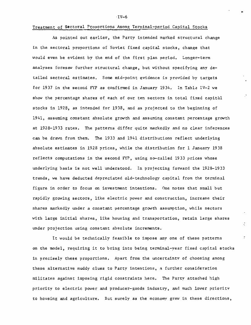
Treatment of Sectoral Proportions Among Terminal-period Capital Stocks

As pointed out earlier, the Party intended marked structural change

in the sectoral proportions of Soviet fixed capital stocks, change that

would even be evident by the end of the first plan period. Longer-term

analyses foresaw further structural change, but without specifying any de-

tailed sectoral estimates. Some mid-point evidence is provided by targets

for 1937 in the second FYP as confirmed in January 1934. In Table IV-2 we

show the percentage shares of each of our ten sectors in total fixed capital

stocks in 1928, as intended for 1938, and as projected to the beginning of

1941, assuming constant absolute growth and assuming constant percentage growth

at 1928-1933 rates. The patterns differ quite markedly and no clear inferences

can be drawn from them. The 1933 and 1941 distributions reflect underlying

absolute estimates in 1928 prices, while the distribution for 1 January 1938

reflects computations in the second FYP, using so-called 1933 prices whose

underlying basis is not well understood. In projecting forward the 1928-1933

trends, we have deducted depreciated old-technology capital from the terminal

figure in order to focus on investment intentions. One notes that small but

rapidly growing sectors, like electric power and construction, increase their

shares markedly under a constant percentage growth assumption, while sectors

with large ini t ial shares, like housing and transportation, retain large shares

under projection using constant absolute increments.

It would be technically feasible to impose any one of these patterns

on the model, requiring i t to bring into being terminal-year fixed capital stocks

in precisely these proportions. Apart from the uncertainty of choosing among

these alternative muddy clues to Party intentions, a further consideration

militates against imposing rigid constraints here. The Party attached high

priority to electric power and producer-goods industry, and much lower priority

to housing and agriculture. But surely as the economy grew in these directions,

IV-7

emerging opportunities would have been seized upon so that outcomes within a

reasonably wide range of variation would have been acceptable. Our modeling

procedures permit us to juggle weights to simulate a variety of computed out-

comes, choosing those with the most attractive composite results. This is

far preferable to imposing rigid proportions that would force the optimizing

procedure to meet specifications requiring needless sacrifices of output.

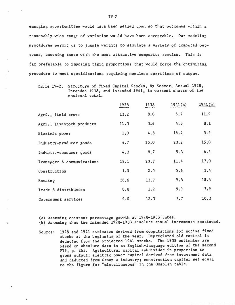
Table IV-2. Structure of Fixed Capital Stocks, By Sector, Actual 1928,Intended 1938, and Intended 1941, in percent shares of thenational total.

1928 1938 1941(a) 1941(b)

Agri., field crops 13.2 8.0

Agri., livestock products 11.3 3.6

Electric power 1.0 4.8

Industry-producer goods 4.7 25.0

Industry-consumer goods 4.3 8.7

Transport & communications 18.1 20.7

Construction 1.0 2.0

Housing 36.6 13.7

Trade & distribution 0.8 1.2

Government services 9.0 12.3

(a) Assuming constant percentage growth at 1928-1933 rates*(b) Assuming that the intended 1928-1933 absolute annual increments continued.

Source: 1928 and 1941 estimates derived from computations for active fixedstocks at the beginning of the year. Depreciated old capital isdeducted from the projected 1941 stocks. The 1938 estimates arebased on absolute data in an English-language edition of the secondFYP, p. 265. Agricultural capital subdivided in proportion togross output; electric power capital derived from investment dataand deducted from Group A industry; construction capital set equalto the figure for "miscellaneous" in the Gosplan table.

6.7

4 . 3

16.4

23.2

5.3

11.4

5.6

9.5

9.9

7.7

11.9

8 .1

5.5

15.0

6.5

17.0

3.4

18.4

3.9

10.3

IV- 8

Evolution of the Post-Terminal Constraint

Economists who have used dynamic optimizing models recognize the importance

of properly specifying terminal conditions. Unconstrained, the "optimizing devil"

will "eat, drink and make merry" in the end, making no provision for a tomorrow

which it does not know exists. In a growth model such as ours, this behavior

takes the form of a failure to invest during the terminal, and perhaps earlier,

periods.

The task of the terminal constraint in KAPROST is, therefore, to maintain

investment at economically reasonable levels even whan the resulting capital

stock will not improve the value of the objective function. If these reasonable

levels could be pre-specified, the form of the constraint would be very simple.

At a minimum, this suggests that it would be plausible to provide for enough

investment in new capacity to continue at the rate already achieved. Hence

the stringency of the terminal constraint will depend on the optimal solution

values, and its form must be built around them.

Table IV-3 lists the various forms of post-terminal constraints experimented

with at various times in KAPROST. The last equation is the one currently in

use. The naming conventions used are described fully in appendix B; the footnote

to the table is only intended as a reminder. Note that common to each form is a

post-terminal growth parameter. Q which allows us to tighten the constraints

parametrically. Further, all are in terms of the increment to capital stock in

the second post-terminal period. As the investment structure in KAPROST requires

two periods for building capital, this increment draws on fixed investment in the

terminal period. (The increment in period T+l contributes to the objective

function, so need not be maintained by constraint.)

Equation 1, the initial version of the constraint, requires that investment

be maintained at a level to cover total depreciation (plus whatever "extra" is

required by the Q parameter). This was felt to be unsatisfactorily low. Given

IV- 9.

Table IV-3

KAPROST Post-Terminal Constraints

increment in new technology capital stock,

for sector i, period t

new technology capital stock, sector i.

period t

as above, for old technology.

depreciation rate, new technology capital, sector i.

depreciation rate, old technology capital

post-terminal growth parameter.

IV-10

a high growth solution, with most of the increment to capital stock in the

final period, the increment provided for capital in period T+2 would be

significantly less than the increment in the previous period. While increasing

X could obviate this somewhat, one can't know how high to set o unless one

knows the solution values. However, altering Q changes the solution, and so

on. It is worth emphasizing that a parameter like 0 is meant to allow the

model user to tighter the constraint, and not to correct flaws in specification.

The second equation calls for the T+2 capital increment to cover the de-

preciation of new capital, and to provide for the same increase from period

T+l to T+2 as the solution calls for from period T to T+l. This is a "same

growth" requirement (with O ^ O indicating somewhat more than same growth),

seemingly very reasonable. However, the optimizer interpreted this quite

differently from the way we intended. Our solutions showed this constraint

raised the cost of increments to capital stock in period T+l so much that it

was optimal to build a very large stock by period T, and then allow it to

depreciate. Hence rather than maintaining investment in the last period, we

had inadvertently eliminated it in the last two periods!

Equation 3 gives our final version of the terminal constraint. The capital

increment in period T+2 must equal the average increment in the preceding six

periods, plus some fraction 0 of capital stock in T+l. The Q parameter is

set equal, initially, to the level of depreciation in each sector. Hence the

constraint requires the model to cover depreciation and to maintain the average

per-period increment in fixed capital. In practice this specification has

worked well. However, one might suggest a different pattern for the weights on

previous capital increments, instead of a simple average. We considered this,

until we realized that any altered set of weights would force investment arti-

ficially away from the periods with the large weights as these periods would be

contributing more heavily to the post-terminal burden. As we had succeeded in

IV-11

maintaining investment expenditure, we felt that the work involved in a more

sophisticated weighting scheme was not justified.

Adjustment of Initial Capital Stock and Capital Productivity

In KAPROST two periods or four years are required to add to capital stock.

This implies that maximum output and capital stock levels for the first two

periods are fixed by the choice of exogenous values for initial capital stock,

initial increments to capital stock, and output-capital ratios. Our initial

experience with values calculated from Soviet data (see Appendix C) revealed

two problems: in most sectors capital stock and productivity ratios would not

allow the model to produce output at historic levels; initial capital stock

and increments would not permit the model to attain historic capital stock

levels in the second period. This indicated shortcomings in the data, especially

the estimate of initial increments to capital, the projects in progress in 1928

before the start of the simulation.

Altering the output-capital ratios for the first two periods to allow the

model to achieve historic production levels is not a major problem. These

coefficients tend to fluctuate in any economy, and we know that in the early

1930's various productivity campaigns caused a sharp rise in output above

expectations. For the remaining four periods the output-capital ratios can be

reduced back to anticipated long-run values.

Altering initial capital stock levels, however, is, in essence, giving

the model extra resources at no cost. Higher levels of output are paid for

by direct demands on production through the input-output matrix, and indirect

demands on production through employment and consumption. Higher initial capital

stocks provide free increments in capacity throughout the model's simulation

horizon, diminished only gradually by depreciation. Clearly this is not acceptable.

We resolved the capital stock problem by increasing the initial increments

IV-12

to capital stock (variable 3 ) , the initial investment pipeline, and by

changing the constraint in which it appears from an equality to an inequality.

This is appropriate for three reasons. First, the increments, if large enough,

will allow the model to achieve historically observed capital stocks for the

second simulation period, 1931-1932. Second, by increasing the initial incre-

ment, rather than the initial stock, of capital, the added capacity can be

obtained only at a price. In terms of the investment dynamics in KAPROST, the

initial increment is in its second investment period (third and fourth year

of construction) in the first simulation period (years 1929-19°'")). As three-

fourths of the cost of investment is incurred in the second investment period,

the model solution must use three rubles of current output for every four rubles

of capital it chooses to build. Taken together with the fragile underlying

evidence on the volume of development projects in progress when the model

solution starts, this formulation appears quite plausible. Third, by requiring

the model to add at most the exogenously specified increment, rather than

exactly the increment, we allow some of these pre-plan projects to be left

forever unfinished. This allows the solution more of a choice in terms of

investment versus consumption in the first period. In actual practice, the

optimizing procedure always chose to invest in the increment, and would have

built even more capital if allowed.

Our precise adjustments are indicated in Tables IV-4 to IV-7. Table IV-4-

shows indices of fixed capital stock by sector on Jan. 1 of the years 1928,

1929 and 1931, with 1928 as a base year. In Table IV-5 we calculate the value

of the initial increment in capital stock needed to permit us to match the

historic levels implied by the indices in Table IV-4. To do this we calculate

the initial stocks of old and new technology capital, and subtract the sum

from the historic stock. In any sector where the required increment exceeds

IV-13

Table IV-4. Actual Fixed Capital Stock, January 1, in millions of rubles

Sector

- iAL

EP

PGi

CG

TC

CO

HO

TD

GS

1928Stock |

8 224

7 594

600

3 017

2 618

11 366

595

22 982

487

5 680

Index

100.0

100.0

100.0

100.0

100.0

100.0

100.0

100.0

100.0

100.0

1929Stock Index

8 553

7 898

676

3 399

2 570

11 583

670

23 478

508

5 920

104.00

104.00

112.67

112.67

98.17

101.91

112.67 ;

102.16

104.23

104.23

1931Stock

9 889

9 132

1 114

5 603

2 508

12 886

1 105

24 258

570

6 652

Index

120.25

120.25

185.72

185.72

95.79

113.37

185.72

105.55

117.12

117.12

Source: Compiled from primary Soviet sources and adjusted as explained

in Appendix A, pp. 23-27. Some of the figures here differ slightly

from those in Table 7 of Appendix A, which reflect recent revisions

and adjustments. Though recomputation of the reference solution

has not yet been carried through, it is not likely to alter

results appreciably.

Sector

AF

AL

EP

?G

CG

TC

CO

HO

TD

GS

(1)

0K1

7 509

701l

569

2 861

2 485

10 959

536

22 086

463

5 519

(2)

0K2

6 259

5 975

511

2 573

2 238

10 188

435

20 397

419

5 210

(3)

NK

1

9 79

954

248

524

452

649

131

1 404

164

246

(4)

Depr.NK1

837

814

223

478

411

603

109

1 305

148

233

(5)

(2)+(4)

7 096

6 789

734

3 051

2 649

10 791

544

21 702

567

5 443

(6)

K1931

9 889

9 132

1 114

5 603

2 508

12 886

1 105

24 258

570

6 652

(7)

AdjustedN32

2 793

2 343

380

2 552

- 141

2 095

561

2 556

3

1 209

(8)

OriginalN"22

315

1 140

194

1 308

697

331

159

479

74

213

(9)ReferenceSolution

N22

2 793

2 343

380

2 552

697

2 095

561

2 556

74

1 209

(1) Initial Stock of old technology capital, Appendix C, Table 6.(2) Column 1, depreciated by sector.

(3) Initial stock of new technology capital, Appendix C. Table 6.(4) Column 3, depreciated by sector.(5) - (2) + (4).(6) Historic 1931 capital stock, Table IV-4 above.(7) m (6) - (5), adjusted increments to capital in period 2.(8) Initial increments to capital in period 2 as originally calculated, Appendix C. Table 5.(9) - max ((7), (8)), increment to capital in period 2 used in reference solution.

Table IV-5. Adjusted Initial Increment to Capital Stock,

AF

AL

EP

PG

CG

TC

CO

HO

TD

GS*

3.15996

2.15026

1.35126

4.26434

5.53981

0.35464

13.07353

0.24250

3.87492

0.90313

979

954

248

524

452

649

131

1 404

164

246

3 094

2 051

335

2 235

2 504

230

1 713

340

635

222

22 752

10 320

1 649

42 032

15 189

5 878

13 068

3 606

6 043

7 710

19 658

8 269

1 314

39 797

12 685

5 648

11 355

3 266

5 408

7 488

7 509

7 01l

569

2 861

2 485

10 959

536

22 086

463

5 519

2.61793

1.17944

2.30931

13.91017

5.10463

0.51538

21.18470

0.14788

11.68035

1.35677

2.67558

1.62549

1.88666

9.72754

5.46371

0.36284

13.06891

0.14742

11.60164

1.04014

2.67558

1.62549

2.30931

13.91017

5.46371

0.51538

21.18470

0.14788

11.68035

1.35677

(1) New technology output-capital ratio, Appendix C, Table 17.(2) New technology capital in period 1, Appendix C, Table 6.(3) = (1) x (2) - New technology output in period one.(4) Historic output in period 1.(5) = (4) - (3) = Old technology output in period 1.(6) Old technology capital stock in period 1, Appendix C, Table 6.(7) = (5) ÷ 6 = adjusted old technology output capital ratio in period 1.(8) Originally calculated old technology output-capital ratio in period 1, Appendix C, Table 17.(9) • max ((7), (8)) - Old technology output-capital ratio used in reference solution periods 1 and 2.

* Government Services output levels are the linearly interpolated values from Appendix C, Table 3.

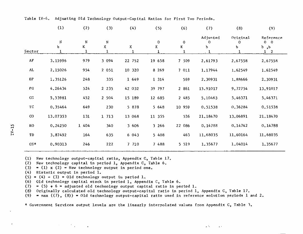
Table IV-6. Adjusting Old Technology Output-Capital Ratios for First Two Periods.

(1) (2) (3) (4) (5) (6) (7) (8) (9)

Adjusted Original ReferenceN N 0 0 0 0 00

b K X X K b b b , bSector 1 1 1 1 1 1_ 1 1 1 2

Table IV-7. Adjusted New Technology Output-Capital for Second Period

(1) (2) (3) (A) (5) (6) (7)

Sector

AF

AL

EP

PG

GG

TC

CO

HO

TD

GS*

X

0

216

7509710

1179

35787

12230

5251

9211

3016

4894

6196

X2

23599

7567

2738

53632

15512

8615

20587

3717

5429

9279

X

N

268490

1559

17845

3282

3364

11376701

534

3083

AvailableN

K2

2 792

2 454

489

2 264

899

2 070

502

3 094

200

1 079

AdjustedNb2

2.45308

—

3.18814

7.88207

3.65072

1.62512

22.66135

0.22657

2.67000

2.85728

OriginalNb2

3.15996

2.15026

1.35126

4.26434

5.53981

0.35464

13.07353

0.24250

3.87492

0.90313

ReferenceN

b2

3.15996

2.15026

3.18814

7.88207

5.53981

1.62512

22.66135

2.24250

3.87492

2.85728

(1) Old technology output in period two, obtained by depreciating values in Table IV-6, Column 5 above,(2) Historic output in period two.(3) = (2) - (1) = New technology output in period 2.(4) Available new technology capital stock in perios 2, obtained by depreciating values in Table IV-6,

Column 2 above, and adding in 70 percent of Table IV-5, Column 9 above (to allow for slowmastering of newly produced capital).

(5) = (3) • (4) = Adjusted new technology output-capital ratios for period two.(6) Originally calculated new technology output-capital ratios for period 2, Appendix C, Table 17.(7) = max ((5), (6)) - new technology output-capital ratios for second period used in reference

solutions.

* Government Services output levels are the linearly interpolated values from Appendix C, Table 3.

IV-17

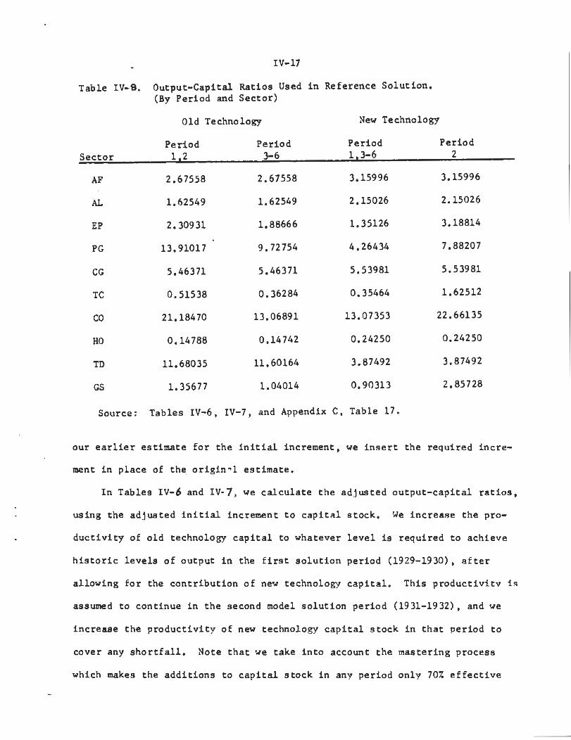
Table IV-9. Output-Capital Ratios Used in Reference Solution,(By Period and Sector)

Old Technology New Technology

Sector

AF

AL

EP

PG

CG

TC

CO

HO

TD

GS

Source:

Period1.2

2.67558

1.62549

2.30931

13.91017

5.46371

0.51538

21.18470

0.14788

11.68035

1.35677

Tables IV-6.

Period3-6

2.67558

1.62549

1.88666

9.72754

5.46371

0.36284

13.06891

0.14742

11.60164

1.04014

IV-7. and Append

Period1.3-6

3.15996

2.15026

1.35126

4.26434

5.53981

0.35464

13.07353

0.24250

3.87492

0.90313

ix C, Table 17.

Period2

3.15996

2.15026

3.18814

7.88207

5.53981

1.62512

22.66135

0.24250

3.87492

2.85728

our earlier estimate for the initial increment, we insert the required incre-

ment in place of the original estimate.

In Tables IV-6 and IV-7, we calculate the adjusted output-capital ratios,

using the adjusted initial increment to capital stock. We increase the pro-

ductivity of old technology capital to whatever level is required to achieve

historic levels of output in the first solution period (1929-1930), after

allowing for the contribution of new technology capital. This productivity is

assumed to continue in the second model solution period (1931-1932), and we

increase the productivity of new technology capital stock in that period to

cover any shortfall. Note that we take into account the mastering process

which makes the additions to capital stock in any period only 70% effective

IV-18

during its first two years. Note further that we never decrease output-

capital ratios below the values calculated in Appendix C. Finally, Table

IV-8 shows the output-capital ratios that are employed for the reference

solution. Note that adjustments occur only in periods one and two.

Desired Characteristics of the Reference Solution

The logical first step in developing a reference solution is to take

the adjusted equations and data, set reasonable values for the consumption

and income parameters, set all objective-function weights at 1.0, relative

to the final period (hence revising upward the weight on consumption in

earlier periods by an appropriate power of the social discount factor),

and then examine the result of the optimization algorithm. It should be

obvious, however, that we still have a great deal of freedom in determining

the characteristics of the solution in these last chosen parameters: average

propensity to consume, fraction of consumption obtained in desired propor-

tions, and objective function weights. Hence the first step, really, is to

attempt to define what properties a reference solution ought to have, and

then see if they can be achieved by varying these control parameters.

Note that we are not imposing a solution on the model; we are no longer

changing any given economic data. Rather we are selecting one out of an

infinite range of solutions inherent in the data. By varying, as Soviet

planners might, the real value of income, the proportion of consumption

satisfied according to consumer desires (as opposed to supply availability)

and the relative importance of consumption in any period versus consumption

in other periods and overall capital development, we can obtain quite different

results. But our range of choice is limited by initial stocks, productivities

IV-19

and the investment structure; these constraints cannot be circumvented.

Our reference, or baseline, solution ought to provide an idealized

illustration of the Soviet economy's potential at the beginning of 1929.

This would mean developing a solution which maintains total real consumption

at 1928 levels, preferably increasing steadily from that base. Further, it

would mean simultaneously building a capital stock by the end of our simulation

horizon in no way inferior to that actually achieved in Soviet experience,

and perhaps even superior to that standard. As should be clear from the

structure of our model, these two goals, higher consumption and higher

capital stock, must ultimately conflict. Hence developing the reference

solution is a process of varying the accessible parameters with a fine sense

of this balance in mind.

Developing the Reference Solution

We present a fairly detailed explaination of how the reference solution

was developed because the process is typical of how all the solutions

discussed below were developed. The cycle of solving the model, examining

the results, and adjusting the parameters for another go, is tedious, but

critical to the successful use of a model of this type. The user learns

how the model reacts, and develops confidence through the reasonableness of

those reactions (or goes back to respecifying the model if those reactions

are inappropriate). Hence we describe the procedure once, leaving the reader

to infer that the same procedure was used to develop solutions for the

historical scenarios on Chapter 6 below.

The logical starting point in a search for a reference solution is to

set the weights on all terms in the objective function equal to 1.0 in the

IV-20

final period. This implies raising the weights on consumption in earlier

periods by the appropriate power of the social discount rate, 10%, so that

consumption in 1929-1930 has a weight of 2.59. Further, the average propen-

sity to consume parameters were set at .5 for the first four periods, and

.7 for the last two periods. Thus real wages were only permitted to be half

nominal wages in the first period, etc. The fraction of consumption satisfied

in fixed proportions was .1, .1, .7, .9, .95 and .95 for periods one through

six respectively. Our previous experience with the model allowed us to

recognize that the solution would permit higher real wages, with consumption

more in line with peasant and worker preferences, in later rather than in

earlier periods. Table IV-9 lists these control parameter values for this

solution, #1, and for the other solutions leading up to and including the

reference solution.

The overall performance of the solution is quite good (see Table IV-10).

Over the 12 years, capital stock increase by a factor of 5, output by a

factor of 31/2 consumption by 21/2. However, the detailed results are clearly

unsatisfactory. There is a great deal of unemployed labor in the first four

periods, rising to almost 20% in the fourth period. More importantly, new

fixed capital is brought into production in sectors where the model finds it

least costly to invest, rather than in those sectors to which the Party

attached highest priority. Notice that the capital stock for the Government

Services sector is nearly half the total. If one examines Appendix C Table 11

one sees that investment in this sector requires a smaller proportion of

output from the Producer Goods sector than any other, and, as Producer Goods

Table IV-9. Parameter Values for Simulations Leading to the Reference Solution

Objective Function WeightsCapital Stocks, Jan. 1, 1941

Agriculture, Field CropsAgriculture, Livestock ProductsElectric PowerProducer Goods IndustryConsumer Goods Industry

Transport and CommunicationsConstructionHousingTrade and DistributionGovernment Services

Consumption1929 and 19301931 and 19321933 and 19341935 and 19361937 and 19381939 and 1940

Consumption ParametersAverage Propensity to Consume *

1929 and 19301931 and 19321933 and 19341935 and 19361937 and 19381939 and 1940

Fraction in Fixed Proportions *1929 and 19301931 and 19321933 and 19341935 and 19361937 and 19381939 and 1940

* These parameters were set identically for workers and peasants.

Table IV-10. Solution #1 Millions of Rubles (Labor Force in Thousands)

IV-23

is the limiting sector for investment, Government Services capital is the

"least expensive" capital that the model can produce. As the weighting of

the objective function values each sector's capital stock equally, the

optimizing algorithm's choice is algebraically impeccable.

In Solution #2 we chose to deal with the problem of the sectoral

distribution of investment. This was done by making a subjective estimate

reflecting the relative priority assigned to each sector by Soviet authorities

in the 1930's. The ten sectors can be grouped quite easily: first priority

went to the heavy industrial sectors, Producer Goods and Electric Power;

second rank went to the two agricultural sectors, field crops and livestock,

along with Consumer Goods (light industry), Transport and Communication, and

Construction; while Housing, Trade and Distribution, and Government Services

were put in a third category. We lowered the weights on the third group to

zero, that is, removed them from the objective function entirely. This

means that only enought capital stock will be built for these sectors to

enable them to provide the output required by exogenous demands and the needs

of more important sectors; in a sense these sectors will be dragged along

by the momentum in the model solution. The weights for the first group

were set to 3.0, making investment here more important than consumption.

The weights for the second group were set just above 2.0, making investment

in them more important than consumption in all but the first two periods

(see Table IV-9).

The summary report for Solution #2 is given in Table IV-11. The same

gross levels of investment, capital stock and output are achieved as in

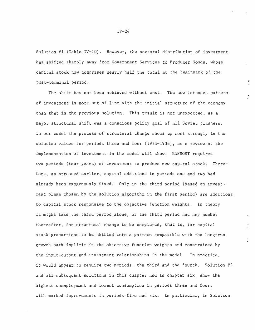
IV-24

Solution #1 (Table IV-10). However, the sectoral distribution of investment

has shifted sharply away from Government Services to Producer Goods, whose

capital stock now comprises nearly half the total at the beginning of the

post-terminal period.

The shift has not been achieved without cost. The new intended pattern

of investment is more out of line with the initial structure of the economy

than that in the previous solution. This result is not unexpected, as a

major structural shift was a conscious policy goal of all Soviet planners.

In our model the process of structural change shows up most strongly in the

solution values for periods three and four (1933-1936), as a review of the

implementation of investment in the model will show. KAPROST requires

two periods (four years) of investment to produce new capital stock. There-

fore, as stressed earlier, capital additions in periods one and two had

already been exogenously fixed. Only in the third period (based on invest-

ment plans chosen by the solution algorithm in the first period) are additions

to capital stock responsive to the objective function weights. In theory

it might take the third period alone, or the third period and any number

thereafter, for structural change to be completed, that is, for capital

stock proportions to be shifted into a pattern compatible with the long-run

growth path implicit in the objective function weights and constrained by

the input-output and investment relationships in the model. In practice,

it would appear to require two periods, the third and the fourth. Solution #2

and all subsequent solutions in this chapter and in chapter six, show the

highest unemployment and lowest consumption in periods three and four,

with marked improvements in periods five and six. In particular, in Solution

Table IV-11. Solution #2 Millions of Rubles (Labor Force in Thousands)

Table IV-12. Solution #3 Millions of Rubles (Labor Force in Thousands)

IV-27

#2, Table IV-11, unemployment in these periods rises above 20%, and peasant

consumption falls sharply from Solution #1.

In order to improve consumption in the two middle periods, a more

detailed examination of the second solution is required. We found that

capital stock utilization in several sectors which contribute to consumption

in fixed proportions, but not to investment - Housing in particular -

was 100%. This bottleneck, would not be removed by raising the objective

function weights. Rather, it is best resolved by lowering the fraction of

consumption which must be satisfied in fixed proportions. This "frees up"

the limited housing stock, which may now be distributed among the larger

number of workers which we expect the model to hire.

Solution #3, Table IV-12, shows the effect of lowering to 0.5 the

fixed proportion component of consumption in periods three and four. In

addition the weight on capital stock in the Electric Power sector was raised

to 3.5 to see if investment could be switched away from the Producer Goods

sector (all control parameter values are listed in Table IV-9) . This second

objective was clearly accomplished, as the largest sectoral capital stock is

now Electric Power.

Examining the consumption and unemployment levels in solution //3 we

see that our selection of control parameters was correct, even if not the

best that could be hoped for. Unemployment is slightly higher in period

three as compared to Solution #2 (24.3% vs 23.7%) but appreciably lower in

period four (22.0% vs 26.8%). Workers consumption for 1933-34 and 1935-36

changes similarly - 15 billion rubles vs 15.4 billion rubles, and 24.8

billion rubles vs 21.7 billion rubles. However, the peasants are virtually

Table IV-13. Solution #4 Millions of Rubles (Labor Force in Thousands)

Table IV-14. Solution #5 Millions of Rubles (Labor Force in Thousands)

Table IV-15. Solution #6 Millions of Rubles (Labor Force in Thousands)

IV-31

unaffected, and detailed examination reveals that capital in both agricul-

tural sectors is fully utilized. Peasant employment is limited by a lack of

farm implements. We decided to attack this problem first by raising the

weight on capital stock for the two agricultural sectors and then by raising

the weight on peasant consumption in the third and fourth periods.

Solutions #4, #5, and #6 are reproduced in summary Table IV-13,

IV-14, IV-15. The weights on capital in both agricultural sectors move

up to 2.5, 2.6 and 3.0, respectively, while that on capital in Electric

Power is lowered to 3.3, 3.2 and 3.2. In Solution #4, this change brings

about a fall in unemployment and a rise in peasant consumption in periods

three and four, when compared to Solution #3. However, Solutions #5 and #6

show no further changes in either employment or consumption. Similarly, the

initial fall in the weight on capital stock in Electric Power causes a drop

in the final capital stock in that sector and a rise in Producer Goods

capital. Solutions #4, #5 and #6 are virtually identical, indicating that

we have found a point on the edge of our convex, feasible set which is

insensitive to those parameters over the ranges we have tested.

As we did not wish to raise the priority of agriculture above that of

the heavy industry sector, we proceeded to the second strategy: increasing

the weights on third and fourth period peasant consumption directly. In

Solutions #7, #8 and #9 we raise these weights to 2.5 and 2.0, 3.0 and 3.0,

and 3.2 and 3.0, respectively. The summary reports for these solutions are

presented in Tables IV-16, IV-17 and IV-18.

Compared to Solution #6, Solution #7 shows little change. However, by

Table IV-16. Solution ill Millions of Rubles (Labor Force in Thousands)

Table IV-17. Solution //8 Millions of Rubles (Labor Force in Thousands)

Table IV-18. Solution #9 Millions of Rubles (Labor Force in Thousands)

IV-35

raising the third and fourth period consumption weights to 3.0 in Solution #8

we cross a threshhold, and succeed in eliminating unemployment in period

four (1935-36). This results in a sharp rise in fourth period peasant

consumption (13.3 to 24.7 billion rubles), at the cost of a small drop in

final capital stock (339.2 to 330.9 billion rubles). Finally, in Solution #9,

by pushing the weight on third period peasant consumption to 3.2, we eliminate

unemployment in that period also, and raise peasant consumption in 1933-34

to reasonable levels. Note here the cost is a further drop in final capital

stock of 4 billion rubles, and a loss of some fourth period consumption.

Solution #9 has most of the properties we listed above as desirable in

a reference solution. It is clear, however, that Producer Goods industry

as a whole would in practice require a larger stock of fixed capital than

Electric Power alone, even given Lenin's stress on electrification.

Our final adjustment, therefore, involves shifting the weights for capital

in these two sectors to 3.1 and 3.0 respectively. The result is a balanced

reference solution which deserves detailed examination.

A Balanced Reference Solution

We have now uncovered an expansion path, consistent with all the model's

parameters, that exhibits a realistic balance between consumption and

accumulation while at the same time drawing into use most of the economy's

productive capacity. Its details are set forth in the accompanying printout,

in the form of five post-solution reports. The five-page summary report

lists objective function elements and displays a number of totals over all

ten sectors for each of the two-year time periods: 1929 and 1930, ....,

1939 and 1940.

IV-36

It then shows gross output levels produced with old-technology capital by

each sector in each period, and similarly the output produced with new-

technology capital by each sector in each period. Another pair of panels

shows the expansion, sector by sector and period by period, of new-technology

stocks of fixed capital. These are primal solution values.

The summary report continues with dual values for capital stocks, by

technology, sector, and period, and for sectoral gross output levels, by

period. These values can be interpreted as indicators of the extent to

which a unit increase in the constraint could increase the value of the

objective function in that period. Large dual valuations are a sign of

bottlenecks. Finally, the summary report tabulates the deliveries to

optional consumption, by sector and period, as a measure of the extent to

which strain in the economy requires deviations from the standard pattern

of consumption by peasants and workers.

For each period the model generates a full set of flow-table entries

like those presented for 1928 and 1933 in Chapter III. These are displayed

for the first period as an interindustry flow report (for the northwest

quadrant), a final demand report (for the northeast quadrant), and a value

added report (for the southwest quadrant). Finally, there is a resource

utilization report giving details on capital and labor utilization in each

sector in each period. For periods after the first, the interindustry and

value added tables are not included in the accompanying material.

PAGE 1

PAGE 2

PAGE 3

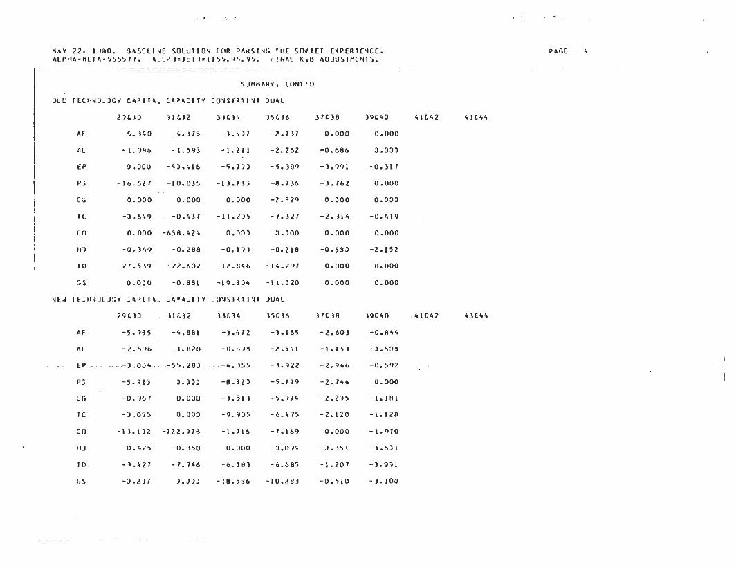
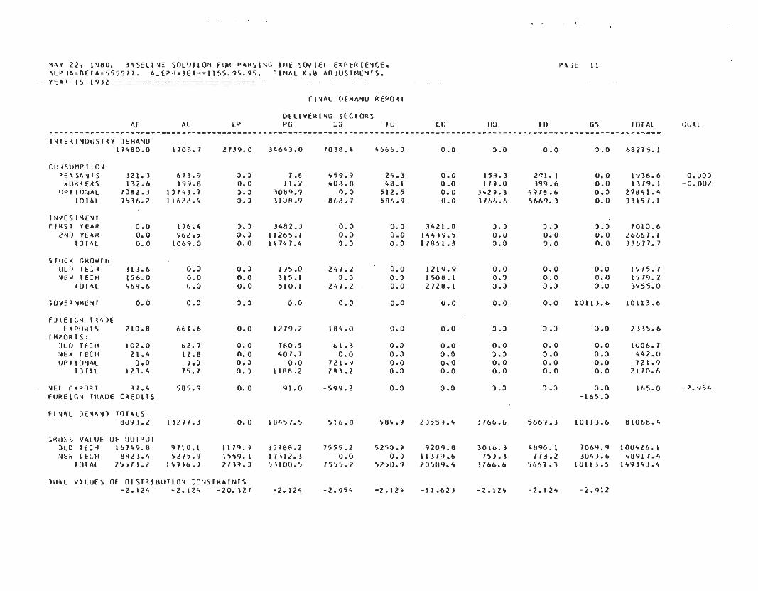
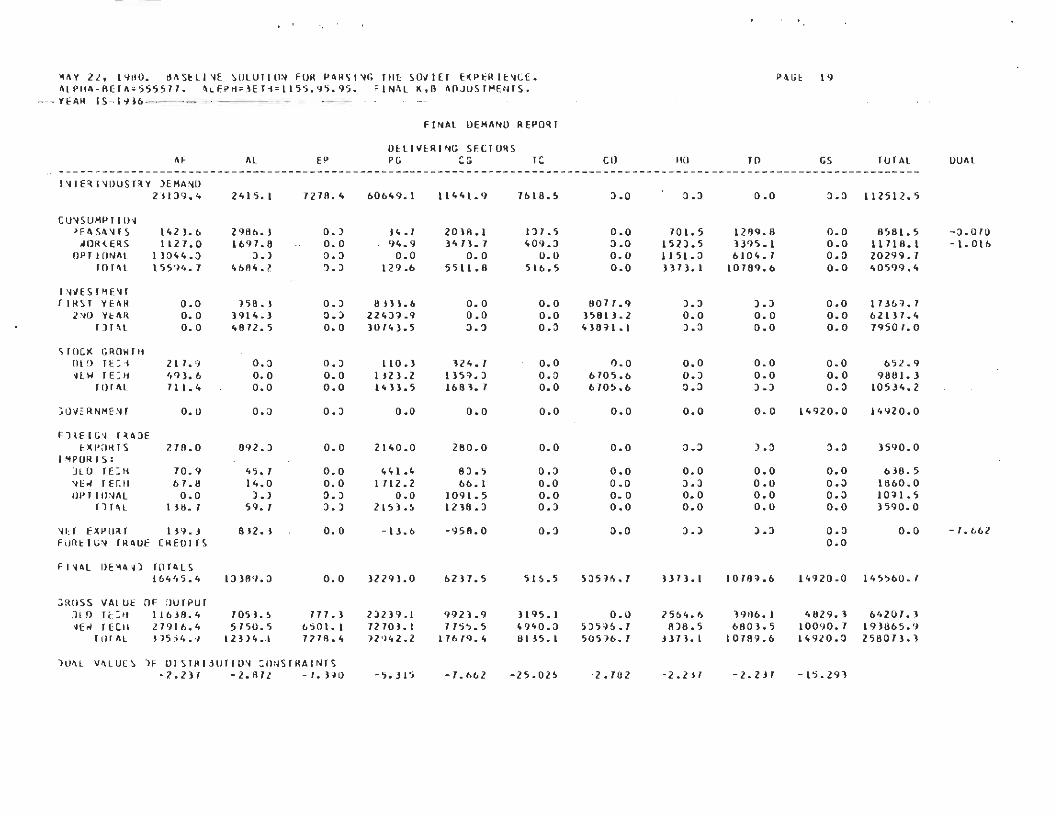
IV-56

The central message of this reference solution is that the Soviet economy

in the 1929-1940 period contained a very substantial potential for output ex-

pansion, under problem-free conditions, without much need for belt-tightening.

Given the base period situation, no model is needed to suggest such a conclusion,

since the resources and growth possibilities were obviously at hand. What the

model does make possible, however, to the extent that i ts assumptions and

calibrations are accepted, are at least some crude quantitative estimates of

the degree and kind of expansion that might have been possible in the absence

of any of the negative developments Chat actually occurred.

In summary form, the expansion path is marked out in the data of Table IV-19

and Chart IV-1. The economy's gross output in period six (1939 plus 1940) could

have been some 3.8 times as large as in Che base period (twice 1928), Deducting

interindustry deliveries, the GNP could have risen from an index of 100 to an

index of 424. Within these aggregates, consumption would have increased some

2.7-fold while investment was rising from an index of 100 to an index of 824.

The stock of fixed capital at the beginning of 1941 would have been five times

larger than i t was at the beginning of 1929. Deliveries to final demand from

the two agricultural sectors would have risen quickly, according to this

reference solution, from a two-year total of 15.0 billion rubles in the base

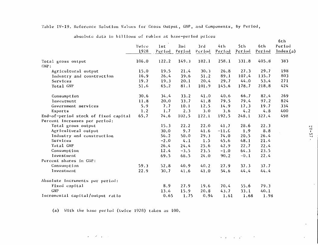
Table IV-19. Reference Solution Values for Gross Output, GNP, and Components, By Period,

absolute data in billions of rubles at base-period prices6th

Twice 1st 2nd 3rd 4th 5th 6th Period1928 Period Period Period Period Period Period Index(a)

Total gross output 106.0GNP:

Agricultural output 15.0Industry and construction 16.9Services 19.7Total GNP 51.6

Consumption 30.6Investment 11.8Government services 5.9Exports 1.2

End-of-period stock of fixed capital 65.7Percent Increases per period:

Total gross outputAgricultural outputIndustry and constructionServicesTotal GNPConsumptionInvestment

Percent shares in GNP:Consumption 59.3Investment 22.9

Absolute Increments per period:Fixed capitalGNP

Incremental capital/output ratio

122.2 149.3 182.1 258.1 331.8 405.8

19.526.419.365.2

34.420.07.71.774.6

15.330.056.2-2.026.412.469.5

52.830.7

21.439.620.181.1

33.233.710.12.3

102.5

22.29.750.04.124.4-3.568.5

40.941.6

8.9 27.913.6 15.90.65 1.75

30.351.220.4101.9

41.041.812.53.0

122.1

22.041.629.31.525.623.524.0

40.241.0

19.620.80.94

26.889.129.7145.6

40.679.514.93.6

192.5

41.7-11.674.045.642.9-1.090.2

27.954.6

70.443.71.61

27.3107.444.0178.7

66.779.417.34.2

248.1

28.61.920482264-0.1

37.344.4

29.7135.753.4218.8

82.497.219.74.8

327.4

22.38.826.421.422.423.522.4

37.744.4

383

198803271424

269824334400498

55.6 79.333.1 40.11.68 1.98

(a) With the base period (twice 1928) taken as 100.

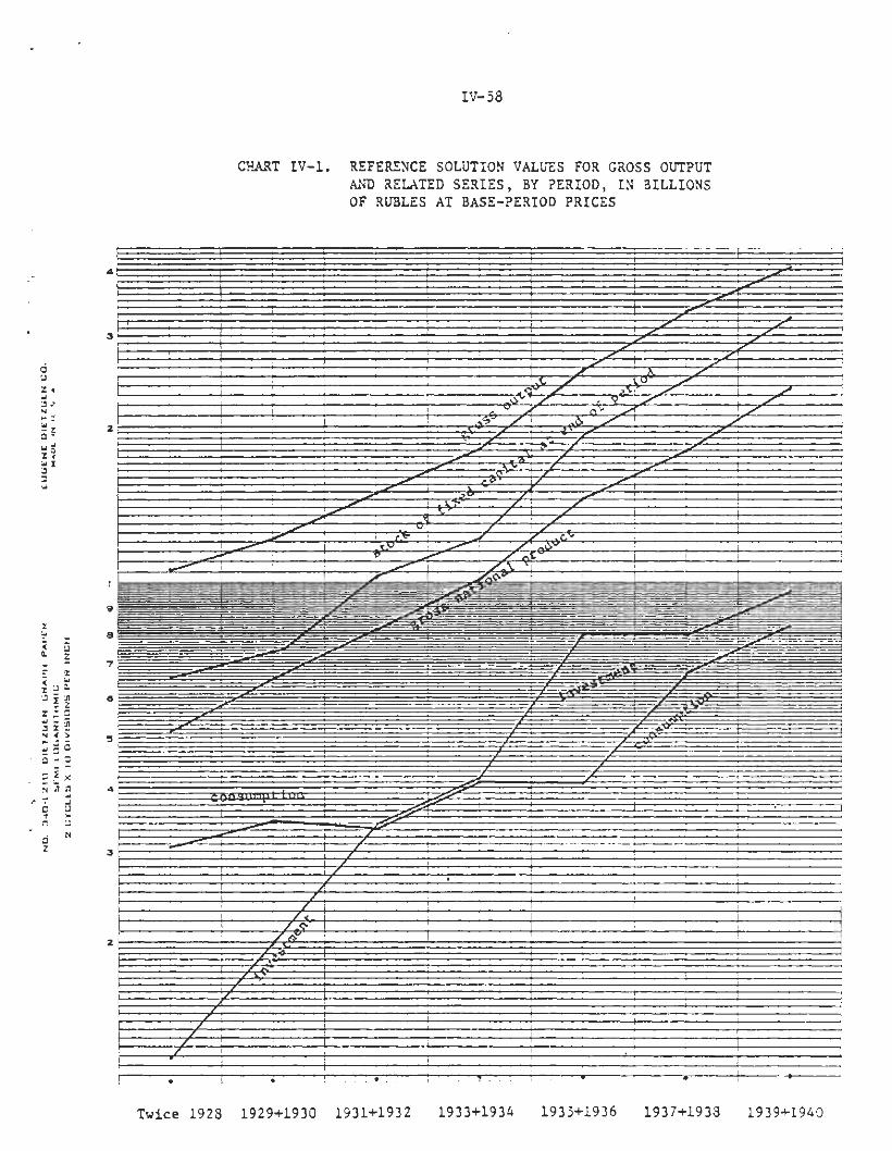
IV-58

CHART IV-1. REFERENCE SOLUTION VALUES FOR GROSS OUTPUTAND RELATED SERIES, BY PERIOD, IN BILLIONSOF RUBLES AT BASE-PERIOD PRICES

Twice 1923 1929+1930 1931+1932 1933+1934 1935+1936 1937+1933 1939+1940

IV-59

period to a total of 30.3 billion in period three, then fallen off slightly

to 27 billion in the next two periods and 30 billion in the sixth period —

double the initial level. Clearly so rapid a degree of improvement in agri-

culture is empirically rather unlikely. Over this same period the output of

the service sectors would have been rising from an index of 100 to an index

of 271, with the growth concentrated in the last three periods. Deliveries

to final demand by the two industry sectors and the construction sector would

have grown rapidly and continuously, reaching by the sixth period a level

eight times higher than the base-period level. Thus would the optimistic

hopes of the system's directors have been realised.

Expansion on this scale would have required a drastic shift away from

consumption and toward investment. Though the absolute level of consumption

would not have fallen, and in fact it would have risen from 30 to over 80

billion rubles, the share of consumption in GNP would have declined from .59%

in the base period to a low of 282 in the fourth period and an apparently

stable share of 37-382 in the last two periods. Conversely, the absolute

amount of investment would have risen from 12 billion rubles to almost 100,

and the investment share in GNP would have increased from 232 to 552 in

period four and 442 thereafter. This 3tress on capital formation would of

course have raised capital stocks very substantially, to more than three

times their size at the beginning of 1929. Comparison of period-to-period

increments in fixed capital and in GNP discloses erratic changes in the incre-

mental capital/output ratio, which rises from 0.65 in the first period to

1.98 in the sixth. These are very low values, by comparison with recent LDC

experience, especially in view of the sectors being stressed. Again it is

evident that this reference solution embodies optimistic parameters.

Given our way of projecting out to 1940 the Gosplan intentions for

IV-6Q

final-demand deliveries to exports and to government services during 1929-1933,

their shares of GNP show modest changes. Exports made up 2.4% of Soviet GNP

in 1928, and this share rises to 2.9% in periods two and three, only to fall

off to 2,2% in the sixth period. Similarly, government services account for

11.4% of the 1928 GNP, a share that would have risen to 12.5% in period two

and then declined to 9% by the sixth period.

Inspection of the dual valuations in this reference solution reveals a

crucially binding constraint in the construction sector in the second period.

It was here that limitations on the amount of fixed capital construction

begun before the plan period but not yet completed, together with the limita-

tion imposed by a two-period gestation period for new fixed capital, would

have placed an insurmountable barrier to further advance. Once past this bottle-

neck in the second period, the model generates construction-sector output

without strain and the dual values fall to negligible levels. There is also

an indication that electric power in the second period was under considerable

strain, but that the strain would have been relieved thereafter. The pattern

of dual valuations varies noticeably under experimentation since these values

are quite sensitive to the linear structure of the model. They are not to

be relied on for a precisely detailed account of sectoral and temporal strains

in this hypothetical reconstruction of a problem-free expansion path.

Through further juggling of weights on individual terms in the model's

objective function (peasant consumption in each period, worker consumption in

each period, and sectoral capital stocks in the final period), we could have

smoothed out some of the sharp fluctuations evident in this reference solution,

and tailored the capital pattern more closely to assumed Party intentions.

The analytic gain would be negligible. Sharp shifts are inherent in linear

programming. As long as one can assume convexity in the model's structure,

IV- 61

a linear combination of two neighboring solutions will be feasible by definition,

so gradual transitions are implicitly available, even if not strictly optimal.

This particular reference solution, for example, builds 161 billion rubles

worth of new-technology capital in the producer goods sector by January 1,

1941, and only 10.1 billion billion rubles worth for the electric power

sector. Examination of Table IV-18 above, recording Solution #9, shows

however that by reversing the weights on capital stock for these two sectors

we can reverse the proportions, creating 114 billion rubles worth of capital

stock in electric power, and 53.4 billion in producer goods. In practice,

the combined total of about 170 billion rubles could have been divided

between these two sectors in almost any desired proportions, within the

overall set of constraints forming the model. The linear programming model

tells us about the zone which bounds feasible territory; it need not be

interpreted as marking out a single, unique, fine-scale "optimal" solution.

It should also be noted that the feasibility of this problem-free refer-

ence solution is affected by its high degree of aggregation. A linear program-

ming approach treats the activities within each sector as completely homogeneous

so that intrasectoral flows are not constrained by technical coefficients, and

intermediate goods are completely substitutable for each other. "It is not

known in advance whether aggregation of sectors, on balance, overstates or

understates the potential achievements of a system. Aggregation permits full

substitution within sectors and thus may overstate production potential. On

the other hand, if as the result of aggregation the average input requirements

imposed in a particularly fast-growing part of the economy are higher than if

that sector were treated separately, the effect is to penalize growth." More-

IV-62

over our use of two-year time periods "...implies complete substitution within

each period. This provides "an additional degree of freedom in breaking

bottlenecks, which is not in fact present..." (though changing from one year to

two years cannot have a decisive influence on evolution over a twelve-year

horizon). "On the other hand there may be compensating disadvantages in tine

aggregation since it forces a kind of synchronization among sectors in each

aggregated time period which in actuality need not be present." Quotes from

R. S. Eckaus and K. S. Parikh, Planning for Growth (1968), p. 154.

In this chapter we have sought to obtain a multisectoral, multiperiod

picture of the way the Soviet economy might have expanded from 1928 through

1940 if the economy's potential had been drawn on as the Party intended and

no difficulties had intervened. Our reference solution appears to mark out

the upper limits of the possible. In historical actuality, however, the

economy suffered a number of serious blows, each leaving its mark on parts

of the system. After sketching the key developments in the next chapter,

we use the model in Chapter VI to decompose the actual record in order to

measure the impact of these events, thus accounting for the differences

between our reference solution and the actual course of events.

VI-1

VI. DECOMPOSING THE RECORD TO MEASURE THE IMPACT OF MAJOR EVENTS

Having compiled broad evidence concerning several major economic

developments in the USSR during the 1930s, we are now ready to insert these

data into the quantitative framework provided by our reference solution for

the 1928-1940 period. Each of the events had an obvious bearing on specific

aspects of the economy. Taken all together, the developments ought to account

for the observed differences between the actual path of the Soviet economy and

the problem-free path spelled out in our reference solution. In theory it

should be possible to derive quantitative estimates of the relative importance

of the individual events in affecting overall results. Ideally, therefore,

we might hope to decompose the actual record, identifying and measuring the

major causal factors at work. This would not be counterfactual history, trying

to estimate what did not happen, and thus should not offend those who, like

Edward Hallet Carr, call for a focus on the interacting complexities of events

as they in fact occurred.

For several reasons, caution is in order concerning the precision of

results to be expected. Soviet statistics for the 1930s were collected under

conditions that tended to produce exaggerations, and were reported in ways that

distorted the record. Even if these defects in the evidence can be overcome,

valuation issues during a period of marked structural transformation introduce

ambiguities that make single-valued answers impossible. In addition, our ten-

sector, six-period model is quite highly aggregated, and though its rigidities

are reduced by a number of technical features, results generated by the model

reflect its oversimplified design. Models with other properties would tell a

different story using the same evidence. We have found, nevertheless, that

extensive experimentation discloses some central tendencies that stand up under

VI-2

a variety of alternative assumptions and over a wide range of parametric

variations. The numerical pattern that emerges is, fortunately, fully in

accord with the qualitative impressions that prevail among most students of

the period. We assert, therefore, that our results provide useful illustrative

detail that throws illuminating light on the forces at work in a very important

and interesting period of structural change.

Of the seven developments in the Soviet economy described in Chapter V

above, the investment drive has already been built into our reference solution,

along with three of the four years of transport strain. The influence of two

other developments: (a) inflation, rationing, and consumer goods shortages,

and (b) political purges and mass terror, was indirect and not easily measured.

We focus, therefore, on the effects of the world depression, of rearmament, and

of agricultural collectivization, each of which can be easily translated into

linear constraints suitable for inclusion in KAPROST. The first two were

clearly exogenous influences; the Soviet government had no control over

the world-wide depression, and little choice but to rearm. However the

decision to collectivize, and its attendant effects, were solely the result of

internal policy decisions. Hence we will examine the impact of each of the

exogenous influences separately, and then combine them to evaluate the total

impact of external affairs on the Soviet economy. We then look at collecti-

vization by itself, as most scholars would agree this was the most critical of

Stalin's policy decisions. Finally we combine all three impacts, hoping to

see a model solution which tracks historical reality fairly well. The difference

between this composite solution and the actual record we attribute to those

influences we have not been able to quantify, and the limitations of our basic

model data.

As noted in Chapter IV, even with the constraints imposed by the model,

an essentially infinite variety of solutions exist. This implies that the results

we present are unavoidably influenced by our judgment as to what would be

VI-3

appropriate and reasonable. We have tried to guide our choices by those

goals which were nearly universal among Soviet policy makers: economic

development through capital investment, with consumption as a secondary

objective.

The Trade Impact of World-Wide Depression

Soviet foreign trade statistics for the 1930s are even more compli-

cated than those of other countries in normal times, as the economy was

undergoing structural change, and price movements were very marked during the

world depression. Many alternative weight years deserve consideration and

index number issues abound. Straightforward, unambiguous computations are not

possible. We take advantage of Michael R. Dohan's painstaking research, and

use his aggregate indices as presented in Table V-4 above.

Table VI-1 repeats Dohan's estimated volume index for Soviet foreign

trade, along with the officially compiled series. Both indexes are derived from

series in foreign-trade rubles, since the USSR does not release data on exports

and imports in domestic prices. The official series corrects for exchange-rate

changes but otherwise reflects current prices. Professor Dohan's series meticu-

lously applies price weights of 1927/28 to quantity data with, fuller and more

consistent coverage than previously employed. As discussed more fully in his

basic report, the corrected series show a smaller drop in imports and exports

after 1931 than displayed by the official series, since the latter reflect both

reduced quantities and lower prices.

While it is literally true that the money value of commodity trade

shrank in the 1930s for both price and volume reasons, the whole KAPROST project

is cast in constant-price terms. Hence we use Dohan's volume indexes to reflect

changes in physical imports and exports over the 1928-1940 period, measured at

VI-4

TABLE VI-1. Volume indexes for Soviet exports and imports,

by year, 1928-1940, 1929 = 100

YEAR

E X P O R T S

OFFICIAL DOHAN

I M P O R T S

OFFICIAL DOHAN

1928

1929

1930

1931

1932

1933

1934

1935

1936

1937

1938

1939

1940

85.7

100.0

112.2

87.8

62.3

53.7

45.3

39.8

33.6

40.8

31.7

14.4

33.1

77.5

100.0

149.5

164.0

128.2

124.6

117.9

105.6

83.7

87.3

78.0

(40.2)*

(138.3)*

107.4

100.0

120.2

125.5

80.0

39.6

26.4

27.4

35.1

33.1

35.5

24.3

35.5

101.1

100.0

123.1

146.1

107.0

66.2

59.7

66.8

68.0

62.2

69.2

(46.8)*

(68.4)*

Sources: Official index derived from absolute figures at the 1950 ruble

exchange rate in MVT, Vneshniaia Torgovlia SSSR ZA 1918-1940 gg

(1960), p.17. Dohan indexes from Michael Dohan and Edward Hewett,

Two Studies in Soviet Terms of Trade, 1918-1970 (Bloomington, Indiana:

Indiana Univ. Int. Development and Research Center, 1973), pp 24 and 27

* Our estimate, as described in text.

VI-5

constant prices. Our reference solution incorporates hypothetical export and

imports obtained by extending planners' intentions in a problem-free environ-

ment; we want to replace these trade figures with quantity flows reflecting

the physical changes that occurred. The additional impact of worsened terms

of trade is analyzed by Michael Dohan; no attempt to enter this range of issues

is made here.

The Dohan series ends in 1938, while our model requires data through

1940. The extension was accomplished by applying the proportionate changes in

the official series for 1939 and 1940 to the last number in Dohan's series.

These estimates are in parentheses in Table VI-1.

While in time it would be possible to derive disaggregated trade series

compatible with KAPROST's four trading sectors, we have initially limited our-

selves to applying aggregate indexes equally to trade in each sector. The model

requires exogenous estimates of exports by sector. Table IV-2 presents these on

a yearly basis for the four exporting sectors, obtained by applying the Dohan

index in Table IV-1 to the 1928 trade numbers in Table III-5. These are summed

in Table VI-3 to yield two-year exports compatible with KAPROST's structure.

Imports in KAPROST are derived first as a ratio of achieved output, and

second, if a net export surplus still exists, as discretionary increments to

critical sectors. We would like to limit total imports to those amounts given

in Tables VI-2 and VI-3. As the model requires net exports plus foreign trade

credits to balance in all periods, by setting foreign trade credits equal to net

imports, this result is achieved. Table VI-3 presents all the data needed for

the trade scenario.

Characteristics of the Trade Solution.

Application of the trade data with no further modifications has a

crippling effect on the KAPROST solution. Capital stock falls to 25% of the

reference solution, sixth period output to 30% of the reference. Examination

VI- 6

TABLE VI-2. Exports by Year and Sector, Total Imports

AGRICULTURE,FIELD CROPS

YEAR

1928 76

1929 98

1930 147

1931 161

1932 126

1933 122

1934 116

1935 104

1936 82

1937 86

1938 76

1939 31

1940 105

(Millions of Rubles

S E C T O R

E X P O R T S

AGRICULTURE,LIVESTOCKPRODUCTS

230

297

444

487

380

370

350

313

248

259

231

92

PRODUCERGOODSINDUSTRY

263

339

507

557

435

423

400

358

284

296

265

106

318 364

)

CONSUMERGOODS

INDUSTRY

50

65

96

106

83

80

76

68

54

56

50

20

69

EXPORT

TOTAL

619

799

1194

1310

1024 .

995

941

844

669

697

623

249

856

IMPORT

TOTAL

792

783

965

1144

838

519

468

524

533

487

542

371

542

1928 Values are from reconstructed input-output Table III-5.

Other values obtained by applying the Dohan index, Table V-l to the 1928 values

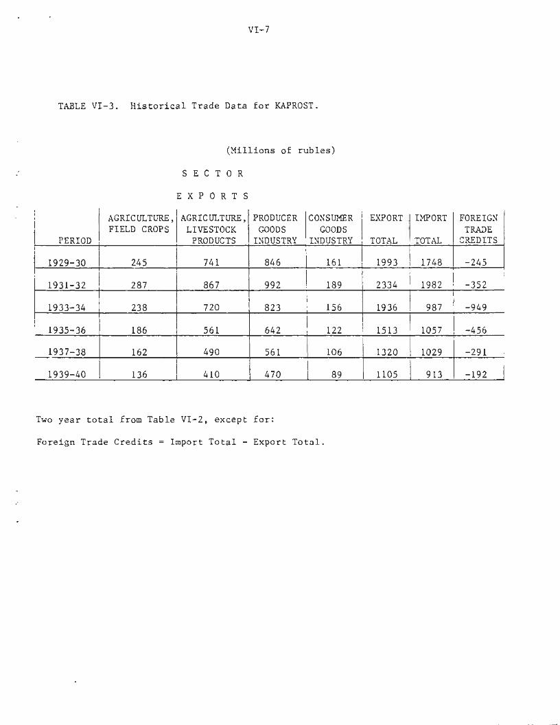
VI-7

TABLE VI-3. Historical Trade Data for KAPROST.

(Millions of rubles)

S E C T O R

E X P O R T S

PERIOD

1929-30

1931-32

1933-34

1935-36

1937-38

1939-40

AGRICULTURE,FIELD CROPS

245

287

238

186

162

136

AGRICULTURE,LIVESTOCKPRODUCTS

741

867

720

561

490

410

PRODUCERGOODSINDUSTRY

846

992

823

642

561

470

CONSUMERGOODS

INDUSTRY

161

189

156

122

106

89

EXPORT

TOTAL

1993

2334

1936

1513

1320

1105

IMPORT

TOTAL

1748

1982

987

1057

1029

913

FOREIGNTRADE

CREDITS

-245

-352

-949

-456

-291

-192

Two year total from Table VI-2, except for:

Foreign Trade Credits = Import Total - Export Total.

VI-8

of the detailed output showed clearly that, given the required import ratios,

the historical level of imports will not support any greater level of economic

activity. As this output is significantly below that which actually occurred

during the 1930s, an adjustment is obviously necessary.

The USSR made some emergency imports of raw cotton, steel, copper, and

a few consumer goods at the start of this period, and many of the early, one-

time imports of machinery and equipment embodied advanced technology that played

a key role in subsequent industrial expansion. But while world depression

clearly reduced planners' flexibility, there is no evidence that any significant

loss of output resulted from an inability to import goods after 1932. Some level

of required imports should be retained to assure that imports are distributed

among all importing sectors, but not so much as to significantly bind the system.

To make this descriptive result precise, the required import ratios were lowered

proportionately until: the largest dual valuation (shadow price) on the balance

of payments constraint is of the same magnitude as the dual value of other con-

straints; and that each period shows some amount of optional imports, but in some

period that number is relatively small.

Table VI-4 presents a comparison of the effect of imposing varying

fractions of the original required import ratios (Appendix C, Table 14) on the

reference solution. The trade data from Table VI-3 are used, but all other data

and parameters are as in the reference solution described in Chapter IV. Note

that as none of the objective function weights have been changed, the objective

function value is comparable across solutions.

Examination of Table VI-4 indicates that we want to impose between 20

and 25% of the original required import ratio. Between these two values, the

dual value of the most stringent balance of payments constraint rises sharply,

VI-9

Table VI-4. Effects of Varying the Required Import Ratios(Billions of Rubles)

Percent ofRequiredImport Ratio

100%

75%

50%

25%

20%

10%

0%

ReferenceSolution

(1)TotalCapitalStock

77.8

118.0

186.8

279.7

290.8

292.7

294.7

294.0

(2)6th PeriodTotalOutput

129.3

169.9

246.9

377.0

407.0

408.4

409.9

405.8

(3)LargestDualValue

219

211

210

?96

10

10

10

9

(4)LeastOptionalImports

0.0

0.0

0.0

0.0

.085

.497

.913

.236

(5)Value ofObjectiveFunction

807.2

934.5

1040.9

1133.2

1207.4

1211.6

1215.8

1219.4

(1) New technology capital stock, January 1, 1941.

(2) Total 1939 + 1940 output.

(3) Highest dual valuation on balance of payments constraintover all six periods, Objective-function increase per unit rise inconstraint.

(4) Smallest total of optional imports over all six periods.

(5) Calculated value of the objective function, summing consumption oversix periods and Jan. 1, 1941 capital stocks over ten sectors.

VI-10

and we begin to see a sharp deterioration in capital stock and output. Note

that with no required imports, or only 10% of the original ratio in force, the

trade scenario is comparable to the reference solution. Hence it is only by

diminishing the flexibility allowed to the optimizing algorithm (or Soviet

planners) that world depression has an important impact on the USSR.

The summary report for the "20% solution" is reproduced in Table VI-5,

and for the "25% solution" in Table VI-6.

The Effects of Rearmament.

Rearmament was felt in the Soviet economy only during the last half of

the 1930s. In evident recognition of the fact that military hardware cannot be

produced without a sizable heavy industry sector, the initial investment surge

focused on producer goods industry. However, military hardware requires military

manpower, and, then as now, the exact division of military expenditures among

branches of industry is difficult to ascertain. Hence we are forced to estimate

some components of military demand from manpower levels, assigning the remainder

to hardware.

Table V-6 above presents the Defense expenditures and Armed Forces man-

power levels for the Soviet Union over our simulation horizon. Note that for the

years 1928-1932 both figures are nearly constant (or unavailable). As a result

we decided to take this minimum force level, 560,000 men and their associated

costs, as implicit in the economy. Thus we assume no changes due to defense in

1929-1932, the first two simulation periods, and we subtract expenditure and

manpower requirements for these men from all later years before calculating the

impact of rearmament.

Where, then, is defense spending to be applied to the economy? We

assumed it would occur in basically two ways. First, troops need food, clothing,

shelter and other basic equipment, both for themselves and their dependents,

Table VI-5. Trade Scenario — 20% of Required-Import Ratio in Force

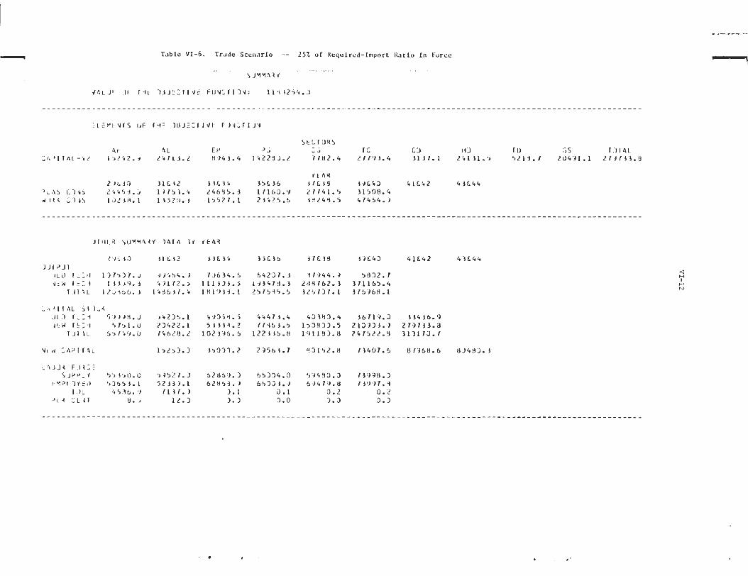
Table VI-6. Trade Scenario — 25% of Required-Import Ratio in Force

VI-13

which implies consumption demand and some capital investment not very different

from that of other sectors of the economy. Second, especially in the late

1930s, an army required deliveries of trucks, tanks, artillery, planes, ships,

etc., all of which come directly from the Producer Goods sector.

In order to provide for the soldiers, we simply employed them through

the Government Services sector of the economy. As shown in Table VI-7, we

take average armed forces manpower in model periods 3 through 6, subtract 560

thousand to determine the increase above minimum force levels and then, using

the output-labor ratio for new technology in the Government Services sector,

determine the increase in demand for such output needed to employ those men.

We add this to historical levels of Government Services output to obtain the

new value of government demand for Government Services in KAPROST. Note this

will not only employ labor equal to the growth in the armed forces, but will

also require the model to build more capital stock for that sector (government

office buildings and army barracks are presumed more or less equal). The wages

paid to the workers will generate increased demand for consumption (soldiers and

workers presumed more or less equal). Note that while army and civilian wages

were certainly not equal, it is real demand for goods we are trying to generate

by this scheme.

The demand for military hardware will be represented by a government

demand for deliveries from the Producer Goods sector. The magnitude will be

the total defense spending less that amount accounted for through increased

government demand for output of Government Services and consumption demand by

the soldiers so employed, as described above. These calculations are shown in

Table VI-8. Note the increased consumption demand by soldiers is obtained by

adjusting the wage payments by the average consumption coefficient, .5 in

periods 3 and 4, .7 in periods 5 and 6.

VI-14

TABLE VI-7. Increased Demand for Government Services

Due to Increased Size of Armed Forces

PERIOD

3

4

5

6

(1)

ARMED FORCES

SIZE

913

1184

1473

3534

(2)

ARMED FORCES

INCREMENT

353

524

913

2974

GOVERNMENT SERVICES(3)

INCREMENT

2871

5075

7425

24188

(4)HISTORIC

9867

11119

12664

14823

OUTPUT(5)

TOTAL

12738

16194

20089

39011

(1) Two year averages from Table V-6, in thousands

(2) = (1) - 560. 560 is the average 1929-1932 force level, in thousands.

(3) = (2) x 8.13315, thousands of rubles. 8.13315 is the output-labor

ratio for Government Services new technology production.

(4) Two year total from Table V-9, the row for Government Services sector,

in thousands of rubles.

(5) = (3) + (4), in thousands of rubles.

VI-15

One further adjustment is required. For the first two periods we

reduce government demand for Government Services to historical levels. In

keeping with the capital stock and capital productivity adjustments described

in Chapter IV we adjust both old and new technology output-capital ratios

in this sector to achieve exactly the historical output in periods 1 and 2

(Table VI-9). In the reference solution we had used linearly interpolated

values from 1928 actual and 1933 planned levels.

Developing a Solution with Rearmament.

As with the trade scenario, direct application of the rearmament data

to the reference solution does not have a salubrious effect; in fact, an in-

feasible solution results. All of the competing demands on output cannot be

satisfied simultaneously, so we proceeded in good Soviet fashion to lower

consumer demand. By lowering real wages to 50% of nominal wages, and reducing

the fraction of consumer demand satisfied in fixed proportions for the last

two periods to half, the model solved. This type of improvement is what one

would expect in a real economy: guns are possible when the amount and variety

of butter is reduced.

The solution still showed some undesirable characteristics: con-

sumption was too low in some periods, and in others included too much of one

sector's output but not enough of others; capital stock was low, and could have

been distributed better; etc. Further adjustments were made to the real wage

and consumption proportion parameters, and to the objective function weights for

capital in agriculture (livestock) and producer goods, as well as third period

peasant consumption. Table VI-10 lists the differences in parameter settings for

this solution versus the reference. Table VI-11 presents our "rearmament only"

solution.

VI-16

(1)

TABLE VI-8

Demand for Military Hardware

(2) (3)Military

(4)

Period

3

4

5

6

Total DefenseSpending

6440

23069

40632

95933

GovernmentServices

2871

5075

7425

24188

ConsumptionDemand

539

991

2180

6807

MilitaryHardware

3030

16995

31027

64983

All values in thousands of rubles.

(1) Two-year totals from Table V-6

(2) From Table VI-7, Column 3.

(3) Table VI-7, Column 1, multiplied by the Government Services wage rate for

each period (Appendix C, Table 10, minus 907.3 thousand rubles (the basic

wage cost for 560 thousand soldiers in 1929) all multiplied by the average

propensity to consume, .5 in periods 3 and 4, .7 in periods 5 and 6.

(4) = (1) - (2) - (3), the government demand for deliveries from the Producers

Goods sector.

VI-17

Table VI-9

Adjustments to Government ServicesOutput-Capital Ratios, Periods 1 and 2

(1) GS Output 1929-1930 6786

(2) New Technology 222

(3) Old Technology 6564

(4) GS Old Technology Capital 1929-1930 5519

(5) Adjusted Old Technology Output-Capital 1.18935Ratio for Periods 1 and 2

(6) GS Output 1930-1931 9279

(7) Old Technology 6196

(8) New Technology 3083

(9) GS Available New Technology Capital 1929-1930 1079

(10) Adjusted New Technology Output-Capital 2.85728Ratio for 1930-1931

All values in thousands of rubles except lines (5) and (10).

(1) Two-year total, Table V-9

(2) First period new technology capital stock (246) from Appendix C, Table 6,

multiplied by first period new technology output-capital ratio (0.90313)

(3) = (1) - (2)

(4) From Appendix C, Table 6

(5) = (3) ÷ (4)

(6) Two-year total, Table V-9

(7) = (3) depreciated one period

(8) - (6) - (7)

(9) From Table IV - 5

(10) = (8) ÷ (9).

VI-18

Table VI-10

Control Parameter Settings: Rearmament vs. Reference

Parameter Rearmament Reference

Objective Function WeightsCapital Stock, 1/1/41Agriculture: LivestockProducer Goods

Consumption1933-34

2.83.2

3.4

3.03.1

3.2

Average Propensity to Consume1929-301931-321933-341935-361937-381939-40

0.40.40.40.40.40.4

0.70.7

Fraction of Consumption inFixed Proportions

1933-341935-361937-381939-40

0.30.40.80.9

Reference solution parameter values from Table IV-8.

Parameters not listed are identical for both solutions

0.50.50.950.95

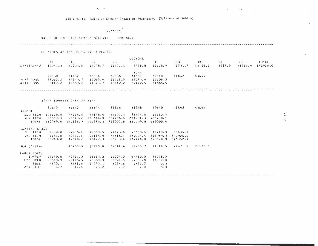
Table VI-11. Solution Showing Impact of Rearmament (Millions of Rubles)

VI-20

Superficially, the impact of rearmament on the Soviet economy

seems severe. Comparing Table VI-11 to the reference solution in Chapter IV,

final capital falls from 327 to 276 billion rubles, and unemployment and con-

sumption worsen in the final four periods. Despite a fair amount of effort, we

were not able to avoid the unemployment and consumption impact, especially the

severe third period result: 1933-34 unemployment of 23.2% versus 0% in the

reference; 1933-34 total consumption of 27.3 billion rubles versus 41.0 billion

rubles (twice the 1928 level of consumption is 30.5 billion rubles). The

capital stock, however does not include 109 billion rubles of military hardware

produced for defense (see Table VI-12 for the calculation of this figure).

Further total output in the sixth period (1939-40) is approximately equal for

both solutions: 405 billion rubles in the reference, 419 billion rubles with

rearmament. KAPROST seems to indicate that while rearmament had a mild cost in

terms of real income, it did not significantly halt development over the 1930s.

Clearly, if war had not intervened, progress in the 1940s would have slowed by

the reduced availability of productive capital, but the economic problems of

the 1930s cannot be blamed on the preparations for war.

VI-21

Table VI-12

Stock of Military Hardware, Jan. 1, 1941

Period

1933-34

1935-36

1937-38

1939-40

Total Milit

(1)Military-Hardware

Expenditures

3030

16995

31027

64983

ary Hardware, Jan. 1, 1941:

(2)Depreciation

Factor to1/1/41

.72723

.80869

.89927

1.0

(3)MilitaryHardware1/1/41

2203

13744

27902

64983

108832

(1) From Table VI-8, Column 4. millions of rubles.

(2) Appropriate power of (1-Depreciation Rate) for old technology

capital in the Producer-Goods sector.

(3) - (1) x (2).

VI-22

The Combined Impact of Trade and Defense

Of the three events whose impact we can quantify and introduce into

KAPROST, the deterioration of trade and the decision to rearm were driven

by exogenous factors. Hence it is of some interest to determine how much

these developments caused the Soviet economy to deviate from a more desirable

path. Table VI-13 combines the preceding adjustments in order to do just this.

All data modifications to implement the deterioration of trade (with 20% of the

required import ratios in force), and all defense expenditures have been in-

cluded. The consumption parameters and objective function weights are set as

in the rearmament solution just discussed.

In examining this solution four things ought to be noted. First, both

consumption and unemployment are maintained at reasonable levels - not as

desirable as the reference solution, to be sure, but not conspicuously poor

either. Second, while capital stock on Jan. 1, 1941 is significantly lower

than that achieved in the reference, this fall is illusory. As noted above,

the total does not include the military hardware produced. Third, sixth period

(1939-40) total output, at 401.6 billion rubles, is insignificantly less than

that achieved in the reference solution. Fourth, combined with the demands of

the military, the balance of payments constraint becomes sharply binding in the

sixth period, with a dual valuation of 284 to 1.

Collectivization in Agriculture

The effect of collectivization on agricultural output and capital stock

is modelled very directly in KAPROST. Actual historical levels of both production

and capital in agriculture are imposed as constraints on the model. We turn

first to estimating these values, then to adapting them to the model, searching

for a representative solution, and discussing the results.

Table VI-13. Combined Trade and Defense Scenario (Millions of Rubles)

VI-24

We have already described briefly the way that collectivization of

agriculture led to smaller herds of livestock and reduced availability

of animal draft power and livestock products, while at the same time raising

the share of agricultural output that was taken for off-farm use. The Soviet

diet, both urban and rural, deteriorated substantially. Detailed analysis is

beyond the scope of this study, but a few computations will illustrate some of

the changes and also supply data so that KAPROST can reflect their impacts.

The shrinkage of livestock herds was a very unfavorable development

but it had the incidental effect of releasing for human consumption some of

the grain and other feed that had been supporting livestock. Without attemp-

ting to trace consumption of vegetables, oilseed cake, etc., one can make crude

estimates of the shift in grain consumption on the basis of readily available

data. Before collectivization about half the total grain crop was consumed

directly as food while roughly a quarter of it went into feed for animals. The

big consumers were horses, especially those of working age, and hogs; smaller

amounts went to cattle, sheep and goats, and poultry. Using summary official

data for herd numbers together with feeding rates per animal as carefully

evaluated by Naum Jasny, Table VI-14 indicates the magnitude of the changes in

grain use by working horses, hogs, and cows (omitting young horses, beef cattle,

sheep and goats, and poultry). The first three columns show the size of the

absolute number, in millions of head, by which the January 1 animal count fell

short of the number on hand at the beginning of 1929, year by year through 1940.

For example, the 22.4 million working horses available in 1929 were reduced by

January 1, 1935, to 10.4 million, a decline of 12.4 million. After 1934 the

horse population rose again, reducing the shortfall. There was restoration in

the number of cows, too, and the number of hogs rose above the base-period level.

VI-25

Applying feeding rates of 450, 245, and 60 kilograms per animal per year,

column 4 shows the amount of grain, in millions of tons, that was released by

these declines in livestock herds. In a period when direct human grain con-

sumption was in the neighborhood of 35 to 40 million tons per year, something

like a fifth of it was made available this way. As Jerzy Karcz pointed out,

"...the entire increase in grain marketings between 1928 and 1933 can be

ascribed to the decline in livestock herds over that period. (The Economics

of Communist Agriculture, Bloomington, Indiana; International Development

Institute, 1980, p. 455).

Since labor was not a constraining input in agriculture, we can focus

on changes in fixed capital as a key factor associated with the output changes

reported in chapter V. Fixed capital in agriculture takes many forms: land,

livestock, barns and houses, wagons, plows, and other equipment, etc., and in

this project it has been subdivided between fieldcrop agriculture and livestock-

products agriculture in fairly summary fashion. It is important to note that in

Soviet agriculture at the beginning of the 1928-1940 period, draft power for

conducting all agricultural activity, in both divisions of agriculture, was

overwhelmingly animal power — horses together with oxen in the South and a few

camels in Soviet Central Asia. We have therefore assigned the value of the 32.6

million horses on hand at the beginning of 1929 — making up about 49% of the

total value of all livestock — to fieldcrop agriculture, leaving the cattle and

cows, hogs, sheep and goats, poultry, and bees to be part of the fixed capital

in the livestock-products division of the agricultural sector. Both stocks de-

clined and rose again, as shown in Table VI-14. The loss of animal draft power

was a major blow to agricultural operations, forcing the Party to provide first

imported and then domestically-produced tractors to fill the gap. In addition

a substantial volume of mechanized equipment in the form of reapers, harvesters,

VI-26

Table VI-14

Reduced numbers of working horses, hogs, and cows, and amount of grainreleased, by year 1929-1940, in millions of animals and metric tons.

Working Grainhorses Hogs Cows Released

On hand, 1 Jan 29 22.8 19.4 29.2

DecrementTo Jan. 1

1930

31

32

1933

34

35

36

1937

38

39

40

1941 8.1 -8.1 1.4 1.7

Sources: Derived from herd data in TsSU, Selskoe Khoziaistvo SSSR (1960), p. 263,

and feeding rates from Naum Jasny, "Soviet Grain Crops and Their Distri-

bution," International Affairs, Oct. 1952, p. 458. The ratio of working to

total horses was .732, .722, and .716 during 1927-29 (KTs 29/30, pp. 530-31).

FYP, II, 1, pp. 332-33 puts it at .696 for 1927/28 and .692 for 1932/33

(intended). The TsSU series for all horses is here multiplied by .7. See

also Jasny, Socialized Agriculture of the USSR, pp. 748-56, esp. p 751.

1.1

3.9

7.6

10.7

12.0

12.4

12.0

11.7

11.5

10.8

10.4

5.2

7.7

8.5

9.5

7.9

2.3

-6.5

-0.6

-6 .3

-5.8

-3 .1

0.7

4.7

6.9

9.8

10.2

10.2

9.2

8.3

6.5

5.2

6.4

1.8

4 .0

5.9

7.7

7.9

6.8

4.4

5.7

4 . 1

3.8

4.4

VI-27

steel plows, etc., was delivered to agriculture, along with a modest number

of trucks.

It has not been possible in this study to compile detailed estimates of

this capital, but a series for the value of tractors is presented in Table VI-15,

column 2. It will be seen that by 1934 the value of tractors on hand, in base-

period prices, had grown to exceed the value of the remaining horses. According

to Jasny's more comprehensive effort to assemble estimates for the sum of all

animal and mechanical power available in Soviet agriculture (displayed in the

graph above in chapter V, page V-6), the 1928 level of total draft power was

not regained until 1938. Though the timing of the changes is uncertain, it is

nevertheless clear that reduced draft power caused serious difficulties over

this period. As for other fixed assets, we have taken refuge in the crude

assumption that stocks remained constant from 1928 through 1940, i.e., that

neither destruction nor construction caused major changes in what was available.

We also make no effort to estimate the value of land as an input, following

established Soviet practice. A more detailed analysis of agriculture might well

distinguish a third subdivision for so-called technical crops (cotton, sugar beets,

oilseeds, etc.), but this too is put aside for another investigation. We are

left, then, with the two total asset series as devices for insertion into our

baseline solution to model the impact of collectivization.

Modifications to KAPROST for the Collectivization Scenario

Imposing on the model the actual levels of capital stock and output in

the two agricultural sectors will also fix investment in, and inter-industry

deliveries to, these sectors - exactly what we require. There are several ways

to incorporate these changes in KAPROST. Our choice was to add a new constraint

placing an upper limit on new technology capital stock, and then adjust capital

VI-28

Table VI-15

Actual fixed assets in fieldcrop and livestock-products agriculture, USSR, by-year, 1928-1940, in billions of rubles at base-priced prices.

Jan. 1

Fieldcrops Agriculture

Horses Tractors Other Total

Livestock-products Agriculture

Herds Other Total

1929

30

31

32

3

3

3

2

.8

.6

.1

.5

0.1

0.1

0.3

0.9

6.2

6.2

6.2

6.2

10.1

9.9

9.6

9.6

4.0

3.1

2.1

1.5

3.7

3.7

3.7

3.7

7.7

6.8

5.8

5.2

1933

34

35

36

2

1

1

1

.0

.8

.7

.8

1

2

4

6

.7

.8

.4

.3

6.2

6.2

6.2

6.2

9.9

10.8

12.3

14.3

1.3

1.5

2.0

2.9

3.7

3.7

3.7

3.7

5.0

5.2

5.7

6.6

1937

38

39

40

1

1

2

2

.8

.9

.0

.l(a)

7.9

7.2

6.7

6.0

6.2

6.2

6.2

6.2

15.9

15.3

14.9

14.3

3.0

3.3

3.6

3.7(a)

3.7

3.7

3.7

3.7

6.7

7.0

7.3

7.4

1941 2.1(a) 5.0 6.2 13.3 4.2(a) 3.7 7.9

(a) Including livestock on acquired territory.

Sources: The horse and non-horse livestock data are derived from estimates in Moorsteen

and Powell, The Soviet Capital Stock, 1928-1962, pp. 105, 107, and 337. The

tractor series is obtained by applying an assumed 5-year life to tractor pro-

duction figures for 1926-1940 in TsSU, Promyshlennosti SSSR, 1964, p. 279, and

linking the resulting stock series to a ruble value at the end of 1928 of 54

million rubles, in KTs 29/30, p. 446. Other assets are valued in 1929 as ex-

plained in Appendix A, and assumed unchanged thereafter.

VI-29

productivity so that if all possible capital stock is built and utilized,

just the historically observed output levels result. Note that this provides

the optimizing algorithm with the option of not building or not using some

portion of agricultural capital stock in any of the periods — with resulting

loss in output as final capital. In practice, however, agriculture is a

binding constraint on the solution and all capital allowed is built.

First we estimate the levels of capital stocks. As old technology

capital stock simply depreciates, and is never increased, its values can be

calculated for each period. New technology capital stock which is carried

over from each period (or which is already established) can be calculated re-

cursively by depreciating the previous years total new technology capital. The

sum of these two items, when subtracted from total capital, yield each period's

additions to new technology capital. Total new technology capital is the sum

of the established portion and additions, while the available new technology

capital counts only .7 of the additions in each period. These calculations are

presented in Table VI-16 for field crops and Table VI-17 for livestock. Note

that the reduction in herds is so great that it, strictly speaking, requires

negative increments to capital stock in the second and third periods. As the

MPS solution algorithm will not permit this type of outcome, we specify values

which lead to zero additions to capital by lowering old technology capital in

those two periods. This tends to underestimate the negative impact of collecti-

vization, as no investment is obviously less costly than positive investment

followed by destruction.

Given capital estimates, we adjust productivity in field crops by

assuming old technology capital productivity is constant, and altering new

technology productivity so that the available new technology capital will

produce the remainder. (See Table VI-18). For livestock, even after reducing

VI-30

Table VI-16

Capital Stock - Agriculture, Field Crops

Period

1

2

3

4

5

6

(1)

K°

7509

6259.3

5217.5

4349.2

3625.4

3153.1

In millions of rubles.

(1) Old technology capital

(2)Established

KN

2591

2215.5

2856.5

4003.9

6798.5

10495.6

(3)Total

K

10100

9600

9900

12300

15900

14900

stock, depreciated from

(A)

zN

-1125.2

1826

3946.9

5476.1

1251.3

1928 value

(5)

KN

2591

3340.7

4682.5

7950.8

12274.6

11746.9

(6)Available

KN

2591

3003.1

4134.7

6766.7

10631.8

11371.5

(2) New technology capital before including additions to capital for that period;depreciated value from previous period, column 5.

(3) Total capital stock, from Table VI-15, column 4.

(4) Additions to capital each period, = (3) -((1) + (2)).

(5) Total new technology capital stock = (2) + (4)

(6) New technology capital stock available = (2) + .7 x (4).

Period

1

2*

3*

4

5

6

(1)

K°

7011

5212.3(5975.5)

4498.6(5092.9)

4340.7

3699.6

3022

Table VI-17

Capital Stock - Agriculture,

(2)Established

KN

689

587.7

501.4

427.7

1159.5

2559.5

(3)Total

K

7700

5800

5000

5700

6700

7300

Livestock

(4)

zN

--

-

931.6

1840.9

1718.5

(5)

KN

689

587.7

501.4

1359.3

3000.4

4278

(6)Available

KN

689

587.7

501.4

1079.8

2448.1

3762.5

In millions of rubles(1) Old technology capital stock depreciated from 1928 value, except see * below.

(2) New technology capital before including additions to capital for that period; depre-ciated from the previous period, column 5.

(3) Total capital stock from Table VI-15, column 7.

(4) Additions to capital each period, = (3) -((1) + (2))).

(5) Total new technology capital = (2) + (4)

(6) New technology capital stock available for production = (2) + .7 x (4)* Value used differs from value obtained by depreciation (in parentheses) for reasons

explained in text.

VI-31

capital stock levels and forcing no additions for two periods, old technology-

capital at original productivity levels produces more than the observed output.

As a result, we summed old and available new technology capital, and divided

this total capital into total output to obtain a common productivity ratio

(Table Vl-19).

The Collectivization Solution

Adjusting the reference solution after applying these modifications

consisted of trying to raise consumption and lower unemployment as much as

possible within the new framework. The average propensity to consume was

lowered to .4 in all periods. The fraction of consumption required to be in

fixed proportions is raised in the fourth period to attain reasonable values

of optional consumption — too large a contribution from trade and distribution

arises otherwise — and lowered slightly in the last two periods to allow more

employment. These parameter changes are presented in Table VI-20.

The resulting solution appears in Table VI-21. Compared to the reference

solution, final capital stock actually increases to 358 billion rubles from 327

billion rubles. This is a reaction to the inability of the optimizing algorithm

to invest in agriculture or to produce output from sectors dependent on inputs

from agriculture, i.e., consumer goods. Producer-goods industry benefits. Of

course consumers pay the bill: consumption is down significantly in all periods

after the first; unemployment is up in all periods, and exceeds 25% in the last

four periods. It should be noted that this is not unemployment in the Western

sense, but indicates the presence of supernumerary laborers and a decline in

labor productivity throughout the economy. Finally, note that sixth period out-

put is down to 320 billion rubles from 406 in the reference solution, an indi-

cation that the lagging agricultural sectors are undermining the whole economy.

VI-32

Period

1

2

3

4

5

6

(1)

X°

18341.9

15289.2

12744.6

10623.6

8855.5

7381.2

Table VI-18

Productivity - Agriculture, Field

(2)Total

X

22752

23599

23126

24072

25393

26317

(3)

xN

4410.1

8309.8

10381.4

13448.4

16537.5

18935.8

Crops

(4)Available

2591

3003.1

4134.7

6766.7

10631.8

11371.5

(5)

6N

1.70209

2.76708

2.51080

1.98744

1.55548

1.66520

In millions of rubles

(1) Old technology output, obtained by depreciating 1928 values

(2) Total output, from Table V-9

(3) = (2) - (1)

(4) Available new technology capital stock, from Table VI-16, column 6

(5) = (3) ÷ (4), adjusted productivity for new technology capital.

Period

Table VI-19

Productivity, Livestock-Products, Agriculture

(1) (2) (3)Total Productive

X K

1

2

3

4

5

6

In millions of rubles

(1) Total output, from Table V-9.

(2) Total capital stock = Old technology capital from Table VI-17 column 1 plusavailable new technology capital from Table VI-17, column 6.

(3) = (l)÷(2), adjusted productivity for old and new technology capital

10320

7567

6172

8203

10320

10498

7700

5800

5000

5420.5

6147.7

6784.5

1.34026

1.34066

1.23440

1.51333

1.67868

1.54736

VI-3S

Table VI-20. Parameter Values: Collectivization versus

Reference Solution

Parameter

Average Propensityto Consume *

1929+19301931+19321933+19341935+19361937+19381939+1940

Fraction of Consumption inFixed Proportions *

1929+19301931+19321933+19341935+19361937+19381939+1940

CollectivizationScenario

0.40.40.40.40.40.4

0.10.10.50.70.850.85

ReferenceSolution

0.50.70.7

0.10.10.50.50.950.95

* These parameters are the same for both workers and peasants.

All other parameters and weights are the same for both solutions

Table VI-21. Solution Showing Impact of Agricultural Collectivization (Millions of Rubles)

VI-35

Trade, Defense and Collectivization

Combining all three influences to approach a composite reconstruction

proved much easier than we had expected. Starting with the combined trade and

defense solution, Table VI-13 above, the agricultural capital and output modi-

fications were added. The resulting solution had several problems: the sectoral

distribution of consumer demand was out of balance, final capital stock was very

low, unemployment was a bit high, and required imports were much too stringent

in the final period.

The necessary adjustments included lowering the required import ratios

to 15% of their initial level, from 20% in trade and defense solution. To

make consumption demand more reasonable, the fraction of consumption required

to be satisfied in fixed proportion was raised to .4 and .6 in periods three

and four (from .3 and .4) and lowered to .8 (from .9) in period six. All other

parameters, including the objective function weights, are identical with those

in the rearmament solution (table VI-11) and the defense and trade solution

(Table VI-13).

The composite reconstruction, combining trade, rearmament and collectiv-

ization is presented in Table VI-22. Note that here the capital stock figures

do not include military hardware. There are three general points to be made

regarding this solution. First, capital stock hold up very well. Second, the

sharp fall in consumption and rise in unemployment in period three appear to

be unavoidable; efforts to alter the model solution to alleviate this damage

were not successful for moderate costs in other objectives. Third, the very

small increment in capital stock in 1941-42 reflects the diversion of resources

away from capital formation and into defense procurement.

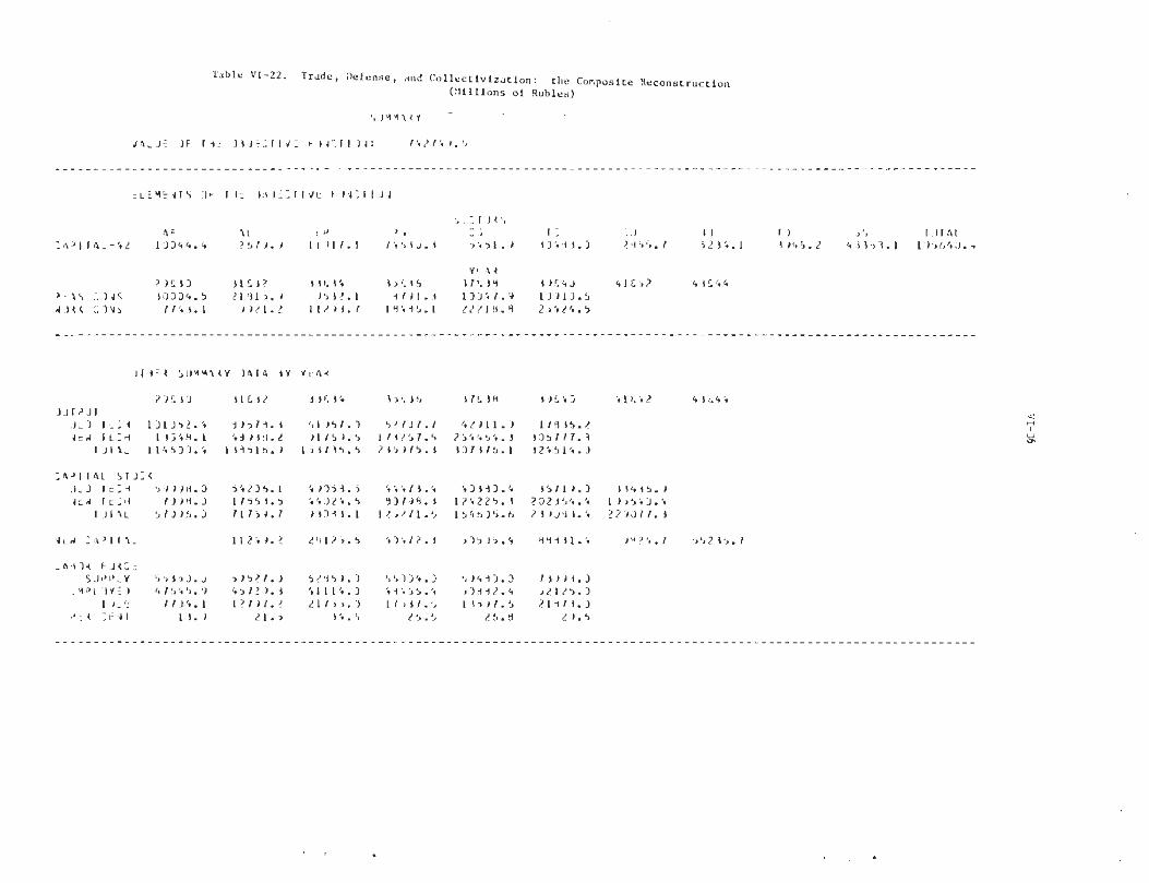
Table VI-22. Trade, Defense, and Collectivization: the Composite Reconstruction(Millions of Rubles)

VI-37

Comparing; These Solutions with the Actual Record

How closely does our composite reconstruction, reflecting the combined

impacts of collectivization, rearmament, and world depression, correspond to

the actual historical record? In many respects we cannot be sure, since important

aspects of the record remain uncertain. But some overall checks are available,

and they indicate that our composite reconstruction matches up fairly closely

with the historical record. For example, comparison of the economy-wide gross

output totals in our composite reconstruction with those compiled above in

chapter V and displayed in Table V-9 demonstrates that our estimates clearly

have the right dimensions. Data for the six periods appear in the first two

lines of the gross output panel in Table VI-23, where it will be seen that our

composite reconstruction starts out slightly below the historical level but

catches up and surpasses it.

This higher growth rate can be traced to two influences. First, the

optimizing algorithum has certain advantages that planners at the time were

unlikely to have had. This supra-normal efficiency we would expect to lead to a

higher growth rate. But it also leads to slack capacity in some sectors in the

first two periods; unaffected by the inertia which haunts real economic systems,

KAPROST does not produce anything it cannot use! Second, as noted above, many

of the negative impacts on the Soviet economy - the purges and terror, the

transportation bottleneck, the initial overinvestment and subsequent waste

were not quantifiable for inclusion in KAPROST. While some of these may have

been picked up in our data (the agricultural output and capital stocks, for

instance), failure to capture them fully will lead to better performance in the

model than in real life.

VI-38

A second confirmation of our composite reconstruction comes from the

correspondence between its capital stock series and the most reliable available

estimate of Societ capital stocks. We show in the first line of the panel

on capital stocks in Table VT-23 the index for gross capital in 1928 prices

compiled by Moorsteen and Powell (The Soviet Capital Stock, 1928-1962, Table

T-28, p. 322), chained to our 1928 ruble figure. The composite reconstruction

tracks the Moorsteen-Powell index closely, though again our estimates are

somewhat below the actual record in the early years and somewhat above it at

the end.

The drastic fall in consumption displayed by our composite reconstruction

from 38 billion rubles in 1929 and 1930 to 32 billion in the next two years and

only 21 billion in 1933 and 1934, cannot be checked against official or Western

estimates, since no continuous estimates are available. Professor Chapman long

ago demonstrated conclusively, however, that the non-agricultural real wage in

1937, after substantial recovery from the most difficult years around 1933, was

17% below its 1928 level (in terms of the 1928 price structure), or 43% below

its 1928 level (in terms of the 1937 price structure). Cf. Janet G. Chapman,

Real Wages in Soviet Russia Since 1928 (1963) , pp. 145-46.

Perhaps interactions within the composite reconstruction that push its

first period total consumption about the 34.4 billion rubles of the reference

solution should be discounted as unrealistic; perhaps even the rise of the

reference solution figure from 30.5 billion in the base period (twice in 1928

level) should be treated as unlikely. These increases reflect KAPROST's

dexterity in distributing output. As capital investment is limited by capacity

bottlenecks in the construction sector, extra output from the agricultural,

housing and consumer goods sectors is delivered to consumers. A more sophisticated

Table Vl-23. Comparing Solutions — Results for Gross Output and Total Capital Stocks,

By Period, in Billions of Rubles at Base Period PricesP E R I O D

GROSS OUTPUT

Actual (Table V-9)

Composite (Table VI-22)

Agricultural Collectivization (Table VI-21

Depression + Rearmament (Table VI-13)

Rearmament (Table VI-11)

World Depression (Table VI-5)

Reference Solution Table IV-19)

TOTAL CAPITAL STOCK, AT START OF YEAR

Actual

Composite

Excluding defense capitalIncluding defense capital

Agricultural Collectivization

Depression + RearmamentExcluding defense capitalIncluding defense capital

RearmamentExcluding defense capitalIncluding defense capital

World Depression

Reference Solution

1929+1930

127

115

)117

119

121

121

122

1929

67.3

67.167.1

1931+1932

151

139

140

148

149

149

149

1931

80.5

71.871.8

1933+1934

169

154

161

171

167

182

182

1933

100.9

93.193.1

1935+1936

231

236

244

250

252

257

258

1935

123.5

125.3128.3

1937+1938

281

307

311

331

340

330

332

1937

160.2

164.6184.3

1939+1940

307

324

320

402

419

407

406

1939

202.6

239.1287.9

1941

265.9

229.1337.9

67.1 71.8 95.7 123.9 183.3 273.0 358.1

65.765.7

65.765.7

65.7

65.7

74.674.6

74.674.6

74.6

74.6

98.098.0

96.296.2

102.4

102.5

125.5128.5

127.0130.0

121.8

122.1

171.1190.8

174.5194.2

191.4

192.5

244.7293.5

250.7299.5

244.9

248.1

262.3371.1

276.4385.2

324.2

327.4

Table VI-24. Comparing Solutions — Results for Total Consumption and Unemployment,By Period, in Billions of Rubles at Base-Period Prices, and Percent Unemployed

P E R I O D

TOTAL CONSUMPTION

Composite (Table VI-22)

Agricultural Collectivization (Table VI-21) 36.4

Depression + Rearmament (Table VI-13)

Rearmament (Table VI-11)

World Depression (Table VI-5)

Reference Solution (Table IV-19)

UNEMPLOYMENT (PERCENT)

Composite

Agricultural Collectivization

Depression + Rearmament

Rearmament

World Depression

Reference Solution

1929+1930

37.7

36.4

36.1

36.2

34.7

34.4

1931+1932

31.7

30.0

35.6

36.2

33.4

33.1

1933+1934

20.9

25.8

32.3

27.5

40.4

41.0

1935+1936

27.3

29.6

31.1

30.8

40.6

40.6

1937+1933

32.3

31.7

37.8

38.4

66.6

66.7

1939+1940

36.3

35.6

47.1

48.4

82.6

82.3

13.9

12.4

9.3

8.7

8.5

7.8

21.5

19.6

13.1

12.4

12.0

11.6

34.5

28.6

14.2

23.2

0.7

0.0

26.6

24.3

4.9

7.7

0.0

0.0

26.8

27.9

7.4

7.0

0.0

0.0

29.6

31.3

0.0

0.0

0.0

0.0

VI-41

model with inventory behavior might have held back some of this for use in

later periods, especially the producer goods. Alternatively, a less efficient

economic system might have lost some of it through waste.

In any case, the fall from 30.5 billion in the late 1920's to 20.9 billion

in 1933 and 1934 represents a 31.5% shrinkage in real consumption. If the 20.9

billion is compared with the third period level of 41.0 billion attained under

the problem-free conditions of the reference solution, the implication is a

49% shortfall in comparison to what might have been.

Another tragic feature of the composite reconstruction is the massive

volume of unemployed labor it involves. The unemployment is organically linked

to the shrinkage in real consumption. Since we have maintained the same physical

labor productivities throughout all the tests from the reference solution on,

the successive constrictions on the economy have made more and more labor

superfluous. The unemployment panel on Table VI-24 shows the results. By

comparison with the reference solution, which made use of all available labor

after the structural shifts of the first two periods were completed, rearmament

altered resource use in a way that generated unemployment in periods three, four,

and five as well. But the impact of agricultural collectivization was far more

severe, making between 24% and 31% of the total labor force unnecessary.

Combining collectivization with world depression and rearmament, our composite

reconstruction generates unemployment levels running from 14% in the first

period to 34.5% in the third, 27% in the fourth and fifth, and 30% at the end of

the decade.

Since by constitutional definition unemployment did not exist in the

USSR, government policy kept the whole labor force at work: on payrolls in

VI-42

non-agricultural occupations or in sovkhozy, as members of kolkhozy, or in

corrective labor camps. Average labor productivity per person in physical terms

fell far enough below its potential to absorb the superfluous labor. Massive

unemployment was thus camouflaged, by contrast with the explicitly exposed

unemployment in the West during the same period.

The results displayed in Tables VI-23 and VI-24 reveal instructive

contrasts. Beginning at the bottom of each panel, one can proceed upward from

the reference solution - our hypothetical best case - step by step to the

composite reconstruction, noting which factors had the strongest impact.

Inspection shows very clearly that agriculatural collectivization dealt the

most serious blow against the economy, far more crippling than the two external

factors of rearmament and world depression. The evidence is especially vivid

in terms of household consumption. Total household consumption over these

twelve years comes to 298 billion rubles in the reference solution; world

depression leaves the total unchanged. Rearmament lowers total consumption by

27%, to 218 billion, and the two exogenous factors in combination have the

effect of restricting consumption to 220 billion. But collectivization of

agriculture reduces the total by 37%, to 189 billion, and our composite

reconstruction shows a twelve-year total for household consumption of 186

billion rubles.

The loss of draft animals and productive livestock did far more than

reduce the flow of livestock products to the population. It forced industry to

deliver tractors and other agricultural machinery to field-crops agriculture

more promptly than had been intended, thus making non-agricultural capital

formation more difficult. It lowered labor productivity in agriculture directly,

and indirectly throughout the economy as well. One sees this in Table VI-23.

VI-43

where, though the total capital stock does not seem severly reduced by the

imposition of collectivization, gross output in 1939 and 1940 is 25% lower in

solutions including collectivization than in any of the others. The capital has

been delivered in less productive uses, and the shift is obtained also at the cost

of severly reduced consumption.

Probably the most important consequence of collectivization, though it

is not directly measurable by KAPROST, was the political tension and pressure

that this "second revolution" spread throughout Soviet society, culminating in

political purges and mass terror. This is the tragic human story that underlies

the laconic figures in our results.

To facilitate comparisons between our composite reconstruction, which is

meant to approximate what actually happened, and the reference solution set forth

at the end of chapter IV, we offer some overall data on GNP components and shares

in Table VI-25. Several striking contrasts are evident. The total GNP in our

composite reconstruction is smaller than in the reference solution over all six

periods, as is only to be expected. The shortfall is modest at first, but it is

15% in the 4th period, 11% in the 5th period, and 21% in the 6th period, as the

negative developments impose their combined effects. Consumption suffers markedly,

as we have seen, but these sacrifices do not serve to make investment larger

in the composite reconstruction than in the reference solution. Collectivization

and rearmament combine to hold investment down, especially in the last two years,

when procurement rises rapidly and fixed capital formation falls from 70 to 21

billion rubles.

The share of consumption in GNP declines from its starting point in both

solutions, as resources are shifted into capital formation. But the belt-

tightening is more severe in the composite reconstruction, where consumption

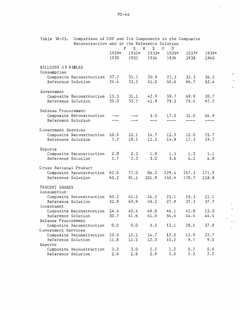
VI-44

Table VI -25 . Comparison of GNP and I t s Components in the CompositeReconstruction and in the Reference Solution

P E R I O D1929+ 1931+ 1933+ 1935+ 1937+ 1939+1930 1932 1934 1936 1938 1940

BILLIONS OF RUBLESConsumption

Composite ReconstructionReference Solution

InvestmentComposite ReconstructionReference Solution

Defense ProcurementComposite ReconstructionReference Solution

Government Services

37.734.4

15.320.0

31.7.33.2

31.133.7

20.941.0

42.941.8

27.340.6

59.779.5

32.366.7

69.979.4

36.382.4

20.797.2

3.0 17.0 31.0

PERCENT SHARESConsumption

Composite ReconstructionReference Solution

InvestmentComposite ReconstructionReference Solution

Defense ProcurementComposite Reconstruction

Government ServicesComposite ReconstructionReference Solution

ExportsComposite ReconstructionReference Solution

0.0 0.0 3.5 13.1 18.5

64.9

CompositeReference

ExportsCompositeReference

ReconstructionSolution

ReconstructionSolution

Gross National ProductComposite ReconstructionReference Solution

10.97.7

2.01.7

62.665.2

12.110.1

2.32.3

77.081.1

14.712.5

1.93.0

86.2101.9

12.514.9

1.53.6

129.4145.6

12.017.3

1.34.2

167.3178.7

22.719.7

1.14.8

171.9218.8

60.252.8

24.430.7

41.240.9

40.441.6

2440

4941

.2

.2

.8

.0

21.127.9

46.154.6

1937

4144

.3

.3

.8

.4

21.137.7

12.044.4

37.8

10.911.8

3.22.6

12.112.5

3.02.8

14.712.3

2.22.9

12.510.2

1.22.5

12.09.7

0.72.3

22.79.0

0.62.2

VI-45

accounts for only one-fifth of the GNP in the last three periods. This extra-

ordinarily low share excludes public consumption, i.e., health care, education,

and municipal services, which account for from 11% to 23% of the GNP, so it is

not quite so shocking. Nevertheless it is clear that the Soviet people bore

a very heavy burden during this period. Half the GNP was channeled into accum-

ulation in 1933 and 1934 under the composite reconstruction, but the investment

share fell off to 42% in the fifth period and dropped to 12% in the sixth, as

defense procurement rose to account for more than a third of the GNP in 1939

and 1940.

For those who may wish to examine further details, sector by sector and

period by period, we conclude this chapter by reproducing the five reports

generated by KAPROST for the composite reconstruction. These are the specific,

concrete estimates of output and resource use that should be compared with

available independent evidence in appraising the accuracy of the composite

reconstruction.

Table VI-26. Solution Values for the Composite Reconstruction. (Millions of Rubles)

Table VI-26. Solution Values for the Composite Reconstruction. (Millions of Rubles)

Table VI-26. Solution Values for the Composite Reconstruction. (Millions of Rubles)

Table VI-26. Solution Values for the Composite Reconstruction. (Millions of Rubles)

Table Vl-26. Solution Values for the Composite Reconstruction. (Millions of Rubles)

Table VI-26. Solution Values for the Composite Reconstruction. (Millions of Rubles)

Table VI-26. Solution Values for the Composite Reconstruction (Millions of Rubles)

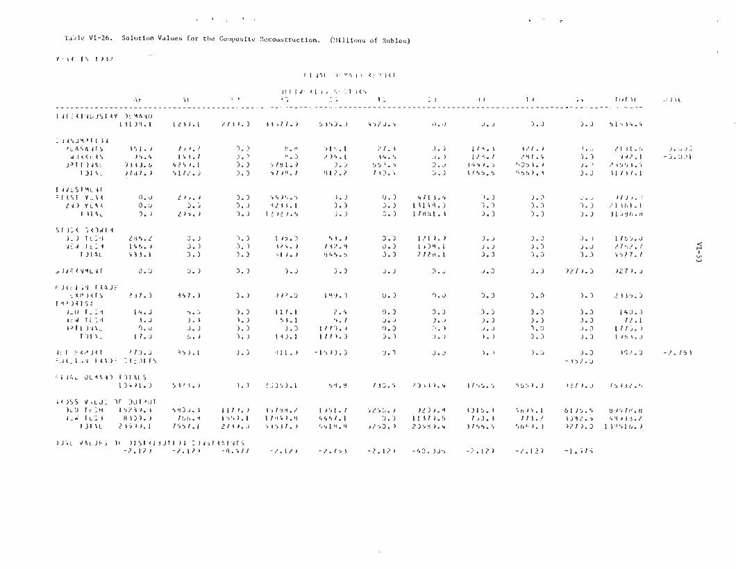
Table VI-26. Solution Values for the Composite Reconstruction. (Millions of Rubles)

Table VI-26. Solution Values for the Composite Reconstruction. (Millions of Rubles)

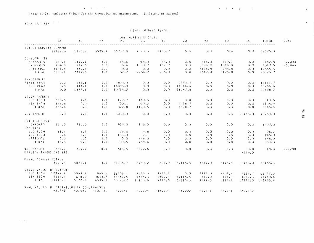
Table VI-26. Solution Values for the Composite Reconstruction. (Millions of Rubles)

Table VI-26. Solution Values for the Composite Reconstruction. (Millions of Rubles)

Table VI-26. Solution Values for the Composite Reconstruction. (Millions of Rubles)

Table VI-26. Solution Values for the Composite Reconstruction. (Millions of Rubles)

Table VI-26. Solution Values for the Composite Reconstruction. (Millions of Rubles)

Table VI-26. Solution Values for the Composite Reconstruction. (Millions of Rubles)

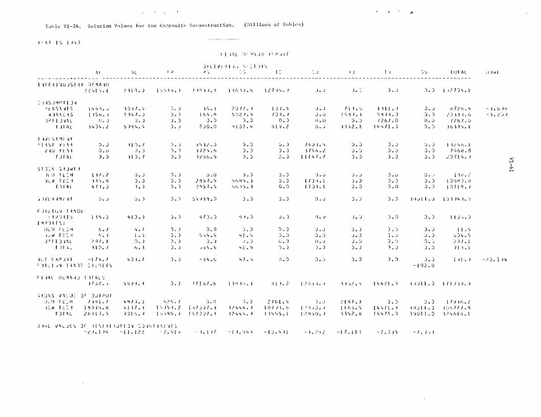
Table VI-26. Solution Values for Che Composite Reconstruction. (Millions of Rubles)

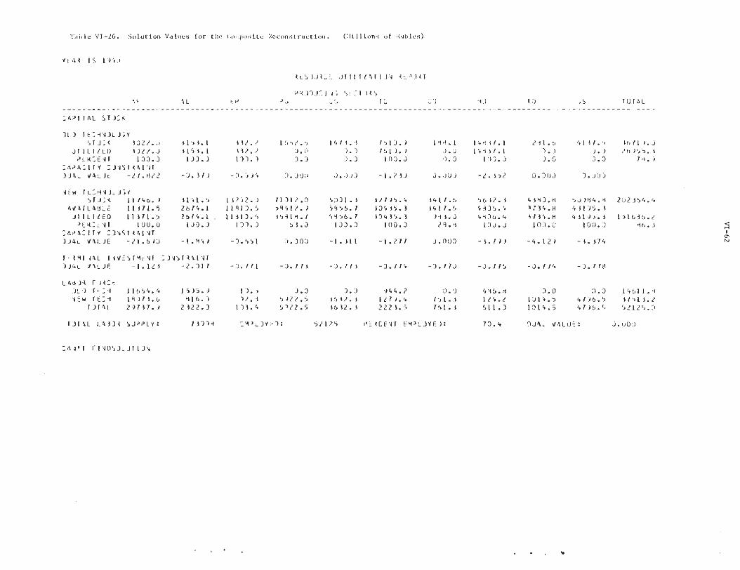
Table VI-26. Solution Values for the Composite Reconstruction. (Millions of Rubles)

Appendix A Statistical Foundations

Pages

A. Dimensions and coverage of the data 3-6

1. Prices2. Dates3. Sectors

B. The 1928 and 1933 flow tables 7 - 2 3

1. Agriculture: field crops and livestock products2. Industry: producer goods and consumer goods3. Electric power4. Transport and communications5. Construction6. Housing7. Trade and distribution3, Government services9. Deliveries to fixed capital

C. Capital stocks 2 3 - 2 7

1. Unadjusted data2. Separating out electric power and construction3. Deducting unfinished construction4. Depreciation

D. Population and labor force 27-341. Population aged 15-592. Sectoral employment, wage rates, and wage bills3. Consumption/income ratios

E. Foreign trade 35-37

1. Exports2. Required and optional imports3. Trade debts

-2-

Appendix table3

Page

1. Agricultural gross output, 1927/28, 1928, and 1932/33, alternativeversions, in millions of rubles. 8

2. Gross output of individual field crops and livestock products, 1928and Plan 1933, in millions of rubles at 1926/27 prices. 10

3. Gross output of census and small-scale industry, 1927/28, alternativereports, in millions of rubles at 1926/27 prices. 13

4. Summary national balance for 1928, as compiled in HP.332, pp. 184-207,in millions of rubles at 1928 prices. 14

5. Transport sector revenues, 1928 and 1933, by mode, in millions of rubles.19

6. Stocks of total fixed capital at the start of 1928, 1929, and 1933, bysector, in millions of rubles at 1925/26 prices. 25

stocks7. Adjusted^of completed and unfinished capital, by 3ector, in millionsof rubles at 1925/26 prices. 27

8. Projected additions to and subtractions from the population aged 16-59,by year, 1928-41, in thousands of persons. 29

9. Hypothetical population aged 16-59 and engaged labor force, by year, 311928-41, in thousands of persons.

10. Annual wage, labor force, and wage bill, by sector, 1928 and 1933. 33

-3-

Appendix A. Statistical Foundations

Dimensions and coverage of the data

Conceptually this study attempts to present its material in real terms,

but its aggregate data are necessarily ruble magnitudes. As much as

possible, they employ base period prices, usually in the form of "1926/27

rubles." Official Soviet statistics using "1926/27 rubles" became increas-

ingly dubious after 1930 or so, as Professor Bergson and many others have

shown. In this study, however, they are only used as measures of the base-

period situation in 1923, or as indicators of expansion intentions expressed

in the first FYP. Soviet prices in the late 1920s may have undervalued

fixed capital relative to current output, and underpriced manufactured goods

relative to primary products, but the general level only rose by two or

three percent from 1926/27 to 1927/28, and the "1926/27 rubles" seem to

provide an adequate set of weights for our purposes. Many targets for the

terminal year of the first FYP were estimated by Gosplan, not only in terms

of "1926/27 prices," but also in terms of values that would reflect sub-

stantial reductions in construction costs and production costs. These

targets in "reduced cost" prices understate the intended physical change in

outputs and inputs, mixing price and quantity changes in ways that would

confound orderly analysis. They are therefore ignored in this study.

In forward-looking planning, ex ante prices have to be employed. One

might conceive of a set of relative prices emerging as the dual to a

terminal-year solution for a vast linear programming problem incorporating

all intervening real structural changes in the economy, but the concept

itself was not available fifty years ago, nor would a sufficiently disaggre-

gated solution be readily obtainable even today. Application of late-year

price weights, reflecting the impact of structural change, is certainly

relevant in measuring growth rates, and if this project were on a larger

scale it could investigate the impact on measured structural change of late-

year weights. Constrained by resources, however, and since our purpose is

to investigate the Soviet economy's potential for producing a new, intended

bill of goods, we can take some analytic consolation from the late Richard

Moorsteen's finding that base-period weights are conceptually the most

appropriate weight3 for aggregation.

Most of the ruble data drawn on for this study were originally in

purchasers prices, including trade markups, freight charges, and excise

taxes, but other evidence, especially that contained in the Materialy po

balansu narodnogo khoziaistva SSR, issued by the Chief Administration for

K

National Accounts in October 1932, makes it possible to derive flow-table

estimates in producers prices for the rows of an input-output table. The

details are set forth below. As for data on capital stocks, Gosplan cots-

piled estimates in "1925/26 prices" for the first FYP, followed by estimates

in almost identical coverage in "1926/27 prices" for the 1929/30 Control

Figures. The national total for October 1, 1928, was put at 70,154 million

rubles in "1925/26 prices" and .69,483 million in "1926/27 prices," a

difference of less than one percent. As with output, the terminal-year, s

target for capital stocks employed here are those assuming no change in

prices, rather than those anticipating marked reductions in construction

costs.

The fiscal year in use at the start of the first FYP covered a twelve-

month period from October 1 through the following September 30. The base

year preceding the plan period therefore ran from October 1, 1927, through

- 5 -

September 1928; the terminal year ended September 30, 1933. In this study,

these two years are referred to as 1928 and 1933. During the plan period,

planning and administration were shifted to a fiscal year coinciding with

the calendar year, beginning with January 1, 1931; the "special quarter" at

the end of 1930 was made the occasion for extra campaigns for over-fulfillment

of plan targets. The shift does not, however, affect the computations in

this project.

The capital stocks on hand and intended are set forth in the FYP by year

and by sector, together with gross investment and annual depreciation estimates,

for the three pre-plan years 1925/26-1927/28 and for the full plan period,

1923/29-19 32/33. Following Eckaus and Parikh, I take the capital stocks on

hand at the beginning of a year as the constraints on that year's activity.

For base period output/capital ratios, therefore, I use active October 1,

1927 capital stocks in the denominator, and base year output levels in the

numerator for each sector. For terminal-year output/capital ratios, I deduce

the October 1, 1932 active stocks implied by growth toward the October 1, 1933

targets and compare them with intended terminal-year output levels. One could

center the capital stocks at midyear for elegance, but the impact on computa-

tions would be negligible.

Our purpose here is to trace large flows among the major sectors of the

economy, including the income and product flows of the usual national accounts, -

but covering also the entries in the northwest quadrant of an economy—wide

input-output table. Soviet research in this direction had already led to

publication of a set of national balances for 1923/24, and fragments of

similar elements and computations appear in the 1929-30 Control Figures and

-6-

in Che first FYP. The Soviet statistical concept of gross output is roughly

similar to gross output in the input-output sense. Plan data are incomplete

at various points, however, so substantial rearrangement and amplification

is required in order to build the two crude tables employed in this study.

The agricultural sector here is divided into field crops and livestock

products; forestry is included with field crops while fishing and hunting

are included with livestock products. Until the mid-1930s, Gosplan included

the construction industry, i.e., the erection of new capital plant and in-

stallation of new capital equipment, in the industrial sector, along with

the industry manufacturing construction materials. For this study I have

attempted to subtract out the fixed assets and current output of the construc-

tion sector to form a separate sector whose capital-forming activities play

a crucial role in the model. Gosplan documents, on the other hand, devote

substantial attention to electrification, and show the electric power

industry separately from other industry. Given its high priority, it is

thus informative to retain electric power as a separate industry. All

remaining industry is divided between producer goods and consumer goods as

explained below. Plan data on the communications sector are here combined

with data for the transportation sector to make up a single sector. Plan

data on capital stocks show very substantial amounts cf urban and rural resi-

dential capital, so a housing sector clearly requires recognition. The flow

of services from this capital must be crudely estimated, however, since Soviet

plan accounts do not recognize this form of output. Gosplan data on assets

make it possible to distinguish two other sectors, one for trade and distri-

bution, and another for government services: education, public health,

municipal services, and government administration. Output measures for these

two sectors are less certain, but the available clues are utilized.

— 7 —

The 1928 and 1933 flow tables

Table 1 presents summary data for several main categories in gross

agricultural output, illustrating the kind of coverage problem that is in-

volved in constructing flow tables for the Soviet economy. The first three

columns related to fiscal 1927/28; the fourth column to calendar 1928; and

the last two columns to the terminal year of the first five-year plan,

figures are reported in "1926/27 prices," except that the fourth column

figures are in 1928 current prices. A glance at the table discloses modest

differences in figures that appear to represent the same item, together with

several gaps. Column six shows the extent to which agricultural targets in

the "optimal variant" were more ambitious than the "basic variant" targest

(in column 5) for agriculture in the first FYP.

The central agricultural activities of growing field crops and producing

livestock products are surrounded by several peripheral activities whose

dimensions have to be deduced from inclusions and exclusions in Soviet sources.

In the FYP, for example, the all-inclusive totals for columns 2, 5, and 6

appear on pp. 162-65 of Vol. I, together with a smaller figure for zemledelie

("agriculture pro p e r " ) . Data for forestry appear in FYP, Vol. I I , part 1,

p, 372, so a residual I take to be for fishing and hunting is precipitated.

For 1927/28 it checks precisely with the fishing and hunting output given in

the 1928/29 control figures (Kontrol'nye tsifry nar, khoz. SSSR na 1923/29

god — hereafter KTs 28/29), p. 398. Further detail appears in KTs 28/29 at

p. 476, and, as entered in column 3, in the control figures for 1929/30

(KTs 29/30), at pp. 534-35 and 422-24. These make the entries in FYP, Vol. II,

part 1, pp. 334-35 more identifiable. All purport to be in 1926/27 producers'

prices, and the generally small variations are not further explained. The

column 4 figures are for calendar 1928 in 1928 prices, from Materialy no

. 8 ,

Table 1. Agricultural gross output, 1927/28, 1928, and Plan 1932/33,

alternative versions, in millions of rubles.

1928/29 First 1929/30control Five-year controlfigures Plan figures

1932balan-

ces

1933basic

targets

1933optimaltargets

Field crops;

All grainsVegetablesTechnical cropsMeadow grassForestry

Total field cropsand forestry

33

11

2

739751901953765

109)

33

11

(10

731032911542765

981)

34

21

(12

551596965105757

974)

42121

(11

449.4842.7046.6072.2411.3

822.2)

54112

(15

2 32649619912596

823)

55112

(17

618085854912596

065

Livestock products:

Meat, poultry, milkFish and gameRaw materialsGrowth of herdsManure

Total livestock products,hunting, and fishing

Total for agriculture,hunting, fishing, andforestry

114368545266244

NA368NA546NA

4 438391642-79350

4 449.2323.5623.2NANA

NA580NA

1 002NA

NA580NA

1 002NA

(5 537) (5 673)

17 646 16 659

(5 742)

18 716

(9 153.9

20 976.1

(8 050)

23 878

(8 741)

25 806

- 9 -

balansu nar. khoz. SSSR za 1923, 1929, i 19 30 g.g. — hereafter MPB, pp. 139,

109, and 185.

The figures in Table 2 provide greater detail on the items making up

the entries in Table 1. They reflect application of average annual 1925/27

prices (from KTs 29/30, pp. 581-32) to physical quantities. The 1923

quantities are drawn from MPB appendix tables, pp. 312-31 and 280-85 (for

timber and firevood). The "optimal variant" targets for 1932/33 are from

the FYP, The computed ruble amounts, in turn, are generally quite close to

those reported for 1927/28 KTs 28/29 and KTs 29/30 if they appear there.

The compilers of MPB assembled remarkable detail on the sources and

uses of all these items, showing physical amounts, ruble amounts, and quo-

tients (average prices) for all but a few cells, with the price varying,

cell by cell, across each row, I multiplied the physical quantities by the

average 1926/27 producer price of each gross output instead, and sunned the

resulting ruble values delivered to each receiving sector in order to obtain

flow-table rows for field crops (including timber and firewood) and for field

crops (including timber and firewood) and for livestock products (including

fish and game, but excluding growth of herds).

No such detail being available in the FYP, I applied the 1928 row struc-

ture to the 1932/33 gross output targets for each crop or product to obtain

an estimate of the anticipated flows to receiving sectors. Since the in-

tended increases of 1932/33 over 1927/28 varied from product to product —

see column 3 in Table 2 •— the composite structure of field-crop deliveries

and livestock product deliveries implied by the plan targets differed sorne-

what from the base-period structure.

-10-

Table 2. Gross output of individual field crops and livestock

products, 1928 and Plan 1933, in million of rubles at 1926/27 price3

All livestock products 5 301 8 185 5b

Sources: For 1928, see text. FYP, II, 1, pp. 338-39 for 1933 targets,

and KTs 29/30, pp. 581-82, for prices, except as noted, (a) FTP, II,

1, P. 335. (b) FYP total nongrain nontechnical minus above estimates for

potatoes and hay. (c) FYP} II, 1, p. 372. (d) FTP, I, pp. 162-65.

(e) 1928 figure raised in proportion to intended growth of herds.

(f) Totals less enumerated items.

-11-

Summary data on utilization of the grain crop, actual in 1927/23 and

intended in 1932/33, appear in a "bread-forage balance" in FTP, II, 1,

page 341. The amounts shown for livestock feed are treated in this project

as deliveries from fieldcrop agriculture to livestock-products agriculture,

except for the feed going to horses, which is an intrasectoral flow. For

the latter I have drawn on Naum Jasny, who analyzed grain crop utilization

in some detail in his Socialized Agriculture o_f_ the USSR (1949) , Note J,

pp. 748-60, supplemented by his paper, "Soviet Grain Crops and Their

Distribution," International Affairs, Oct. 1952, pp. 452-59. He shows annual

feeding rates for adult horses of 464, 593, 458, and 408 kilograms per head

from 1925/26 through 1928/29 on p. 753, and suggests an average for the

period of "about 450 kilograms" (p. 453), evidently considering 1926/27

atypical. Multiplying 21.4 million head of working horses (FYP, II, 1, p. 38)

by 458 yields 9.8 million tons of grain, 40.21% of the total used for feed

in 1927/28; the same share is assumed for 1933.

In connection with actual developments after 1928, one might assume

lower feeding rates under the stress of collectivization except that Jasny

notes (p. 458) "...a counteracting factor is the fact that large farms

generally tend to use more concentrated feed for their animals than small

farms...," and his further observation (p. 755) that "...the great shortage

of all kinds of draft power would have necessitated more work and more con-

centrated feed per work animal." Applying the same feeding rate and noting

the fall in the total number of horses from 32.6 million on Jan. 1, 1929 to

14.9 million on Jan. 1, 1935, suggests a proportionate fall in grain consumed

by working horses, thus releasing as much as 5.6 million tons of grain

annually for human consumption.

- 1 2 -

Five-Year Plan documents provide abundant data relating to industry

but, a s . with -agriculture, many i3sues of definition and coverage complicate

an effort to prepare unambiguous estimates for flow tables. The most de-

tailed stat is t ics came to Gosplan and TsUNKhU from so-called "census industry,"

especially those enterprises whose activities were planned by Vesenkha, There

were, however, enterprises in census industry not under the supervision of

Vesenkha, and there was a good deal of activity in so-called "small scale

industry." Table 3 records some gross output totals from our four principal

sources showing the diversity of summary data. Output figures are further

complicated by a distinction between gross output and net output (literally

translated as "the trade part"), which differed appreciably from source to

source , product to product to product, and year to year. Finally, industry

in the USSR has long been thought of as producing either producer goods

(Group A) or consumer goods (Group B), a distinction associated with the con-

trast between "heavy industry" and "light industry." Responsible Soviet

economists and statisticians readily recognized that some consumer goods were

produced in heavy industrial enterprises, and that some of the products of

light industry were consumed as intermediate inputs by industry, thus becoming

in fact producer's goods. They found in practice that neither classification—

by type of product or by type of producer — can be imposed and maintained

without overlap, ambiguity, and compromise.

The national balances released in 1932 employed a conceptual framework

providing a great deal of the structural information required for a present-

day input-output table. Within this framework a substantial volume of

detail is presented in appendix tables, extremely revealing for developments

in 1928, 1929, 1930, and (to some extent) 1931. Table A shows the main

categories appearing on both the sources and uses side of the annual balances;

-13-

Table 3. Gross Output of Census and Small-scale Industry, 1927/23,

Alternative Reports, in millions of rubles at 1926/27 prices.

Census industryPlanned by VSNKhOther

Small-scale IndustryAll industryExcise taxes

(1)1928/29 KTs

13 333

2 69516 5281 505

1310

23

161

(2)FYP

382909973034916396

(3)1929/30 KTs

14 13111 0673 0644 962

19 093

(4)(3) ad1.

14 11511 0673 0483 412

17 5271 402

(5)1932 Bal

19 245.0

5 868.725 113.71 463.0

Total incl . excise taxes 18 033 18 312 18 929

Sources: KTs 1928/29, pp. 400, 402; FTP, Vol. I I , pt. 2, pp. 84-85; KTs 1929/30,pp. 429, 592; MPB (1932), p. 185.

Note: The 1929/30 KTs data include flour millions, Col. 4 deducts estimates for flour-milling given in FYP, Vol. I I , pt. 2, pp. 120-21.

detailed entries for component elements are placed in the same format. At

the bottom of Table 4 is an indication of the adjustments decided on for use

in the present study. Losses (line 12) are subtracted from both sides of

the balance. Supplies on hand at the beginning of the year are. subtracted

from supplies on hand at the end of the year to obtain a measure of deliveries

to inventory. Total deliveries of domestic production (net of losses) to-

gether with imports are then traced as going to interindustry receivers (line 8)

and to the usual final demand claimants: households, government, investment,

exports, and inventory. The MPB s ta t i s t ic ians were meticulous in estimating

the incidence of trade-transport markups, excise taxe3, and import duties;

as a result deliveries in purchasers prices can be reduced to deliveries

in producers prices with fair precision. The MPB s ta t i s t ic ians placed hunting

and fishing with agriculture but placed forestry with industry; detailed data

on roundwood and firewood enabled me to shift forestry over to join the field-

crops part of agriculture. Following established Marxist-Leninist theory

-14-

Table 4: Summary national balance for 1928 as compiled in MPB 32, pp. 184-207, in

millions of rubles at 1928 prices.

Sources

1 Total supplies atbeginning of year

2 Annual productionat producers prices

3 Trade-transport markings

4 Excise taxes

5 Imports

6 Import duties

7 Total available atpurchasers prices

Uses

8 Total consumedin production

9 Total consumed bypopulation and institutions

10 Total delivered forfixed investment

11 Exports

12 Losses

13 Total supplies at endof year

14 Total distributed inpurchasers prices

15. Total supplies minusstarting supplies (13-1)

Total deliveries at purchasersprices (8+9+10+11+15)

Deductions (3+4+6)

Total deliveries at producers

prices (2+5-12)

Products Products of Products of Wholeof industry agriculture construction economy

-15-

the MPB statisticians did not, however, provide much information on the

output of nonmaterial economic activities; these had to be estimated in

ways explained below.

After a good deal of frustrating experiment i t has seemed best for

present purposes to make no use of Soviet figures for net output, relying

instead on the rather detailed appendix material in the 1932 MPB providing

breakdowns between "means of production" and "objects of consumption" as

they were , delivered to major sectors of the economy. Using these two cate-

gories, two rows can be developed for industry. Because of i ts high

priority, the electric power subsector of heavy industry is here separated

out from the producer goods row. At the same time i t is necessary to draw

as much as possible from the FYP itself for gross output figures relating

to actual 1927/28 and to intended 1932/33, since they provide the most con-

clusive evidence on the planners' own figures and intentions. These are

conveniently summarized in a table in FYP, I I , 2, pp. 78-79, shoving effective

demand for industrial goods, in millions of rubles at purchasers prices:

Demand for means of production:Agriculture and forestryIndustry and electrificationTransportCommunicationsTradeCommunal economyHousing construction"Nonproductive" commissariats

Total demand for means of production

Demand for means of consumption:Urban populationRural populationCollective consumption, by "nonproduc-tive" commissariats and other pro-organizations

Total demand for means of consumption

1927/28

7066 37292480290178460125

basicvariant1932/33targets

1 85210 3931 876103388350

866341

optimalvariant1932/33targets

1 95810 9002 280108481514

985408

9 135 16 169 17 634

33

1_

7

062318

010

390

45

1

11

474077

520

0.1

45

1

11

866441

617

924

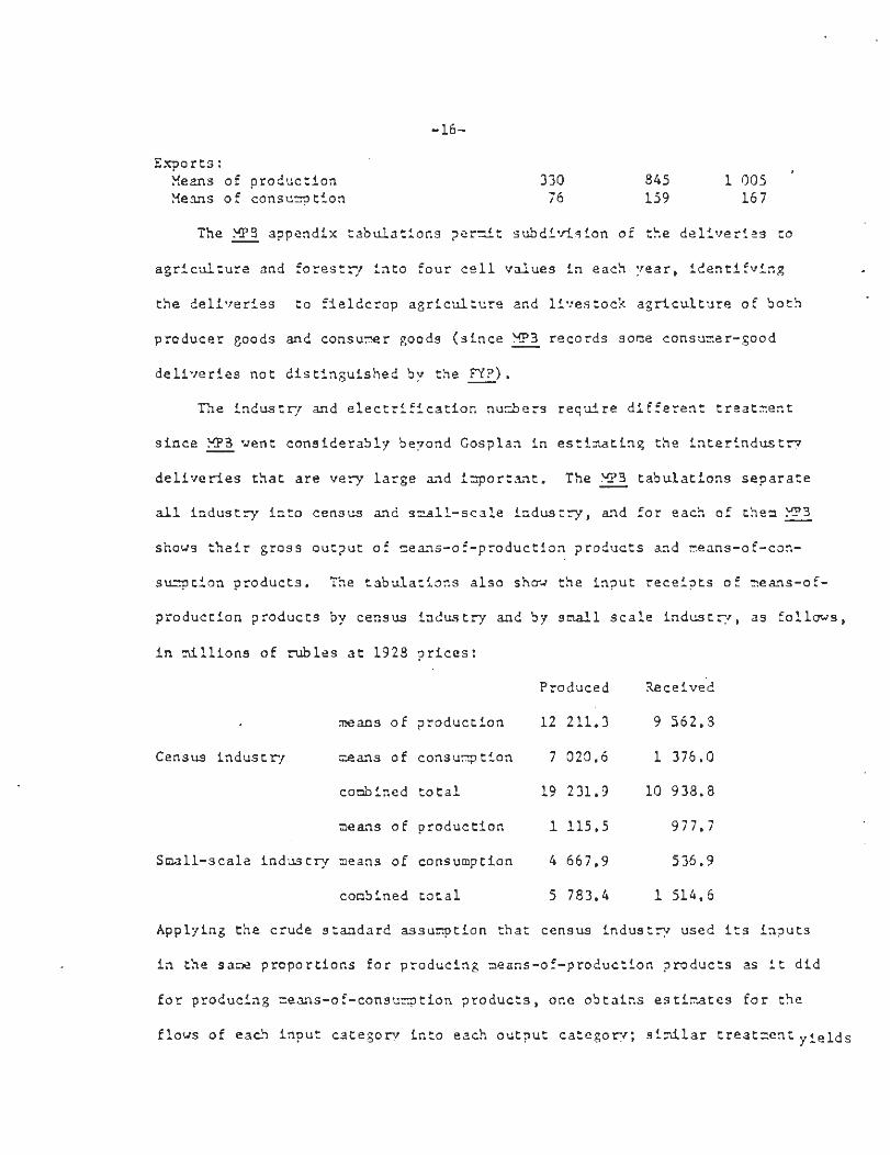
- 1 6 -

Exports:Means of production 330 345 1 005

Means of consumption 76 159 167

The MP3 appendix tabula t ions permit subdivision of the de l ive r i e s to

agr icu l tu re and forest ry into four c e l l values in each year , ident i fy ing

the de l ive r ies to fieldcrop agr icu l tu re and l ives tock ag r i cu l tu re of both

producer goods and consumer goods (since MP3 records some consumer-good

de l ive r i e s not dis t inguished by the FYP).

The industry and e l e c t r i f i c a t i o n numbers require d i f fe ren t treatment

since MPB went considerably beyond Gosplan in est imating the in t e r indus t ry

de l ive r i e s that are very large and important. The MP3 tabula t ions separate

a l l industry in to census and smal l -scale indus t ry , and for each of then MPB

shows the i r gross output of means-of-production products and means-of-con-

sumption products . The tabula t ions also show the input rece ip ts of means-of-

production products by census industry and by small scale indus t ry , as follows,

in mil l ions of rubles at 1928 p r i c e s :

Produced Received

means of production 12 211,3 9 562.8

Census industry means of consumption 7 020.6 1 376.0

combined t o t a l 19 231.9 10 938.8

means of production 1 115.5 977.7

Small-scale industry means of consumption 4 667.9 536.9

combined total 5 783.4 1 514.6

Applying the crude standard assumption that census industry used i ts inputs

in the sane proportions for producing means-of-production products as i t did

for producing means-of-consumption products, one obtains estimates for the

flows of each input category into each output category; similar treatment yields

-17-

flows in small-scale industry as well. Adding census industry and small

scale industry together yields the following deliveries:

toproducer

goods

toconsumergoods

From producer goods 6 261 4 280

From consumer goods 977 936

These total 12,454 million rubles, almost twice the 6,372 million Gosplan

shows for 1927/28, but the added amounts appear plausible as intrasectoral

flows and at least crude cell values are needed for the interindustry tech-

nology matrix. A cell value for electric power is derived below.

For transport and communications, MPB estimates provided a percent

division between producer and consumer goods that is applied to the FYP? fig-

ures. For the construction sector MPB estimates are used instead of the

FYP figure which is limited to housing construction alone. The FYP figure

for "communal economy" is accepted as applying to producer goods used in the

sector supplying housing services to the urban population. For trade, the

FYP? figure is divided in MP3 proportions. The two FYP figure3 for "unpro-

ductive commissariats" are taken as applying to the government services

sector. The urban and rural consumption figures are subdivided in MPB

proportions since here again the MPB statisticians had more thorough break-

downs. The FYP export data are accepted as given. An estimate for additions

to stock is derived from year-end figures for 1926/27 and 1927/28, sub-

divided in MPB proportions. Finally, since all these figures are for domestic

production plus imports, measured in purchasers prices including a trade-

transport markup and excise taxes, they have been reduced across each row

by uniform percentages derived from the detailed MPB appendix information.

-18-

Industry rows for the 1933 flow table are built on the gross output

targets for producer-goods and consumer-goods production, assigned in the

ways intended by Gosplan, but subdivided in the proportions uncovered for

1928 by the M?3 s ta t is t ic ians . This approach fails to capture some of the

structural change that lay within the aggregates published in the first FYP

but at least i t reflects the diverse growth intentions planned for combined

deliveries to individual receiving sectors.

Deliveries of electric power can be deducted from the producer goods

row on the basis of scattered information in the first FYP and elsehwere.

The MPB study presents an electric power balance for 1928 in kilowatt-hours

and in rubles (p. 267); i t s KWH figures conform closely to those in FYP, II ,

1, p. 66, as indicated in the following tabulation:

1928MPB FYP 1933 basic 1933 optimal

Receiving sector:

Agriculture

Census industry

Transport and communications

Communal and consumption uses

Station use and transmission losses

Total 5 003 5 050 17 000 22 000

The 1933 figures in parentheses distribute the unstated optimal residual in

basic-variant proportions. The deliveries to census industry can be divided

into deliveries for means-of-production industry and means-of-consumption

industry on the basis of detailed absolute estimates for 1927/28 in the

TsUNKhU s ta t i s t ica l handbook, Narodnoe khoz. SSR: stat . sprav. 1932, pp. 40-41.

The MPB ruble data are used for 1928 and a 1928 price of 91.2 rubles per

1000 KWH is used to get 1933 ruble estimates.

3

1

45

268

111

039

540

35

3 130

140

815

9 30

11

1

2

210

700

400

870

820

(254)

15 000

(484)

(2 262)

4 000

-19-

Entries for the input column of the electr ic power sector are not readily

available from plan documents, so I have applied the estimates developed by

the Indian S ta t i s t ica l Inst i tute for India in 1959/60, as resorted by Richard

S. Eckaus and Kirit S. Parikh in Planning for Growth (1963), p. 60. The

principal flows involve coal, ra i l transport of coal, and the diagonal cell

(including losses).

The f i rs t FYP lacks financial detail for a transport and communications

flow-table row, but some dimensional evidence is available from other sources,

especially a s t a t i s t i c a l publication issued by the transport commissariat

setting forth the plan's transport aspects (though mainly for the "basic

variant"), Actual and expected revenues from freight and passenger service

by the several carriers are set forth in Table 5; the dominant role of the

railroads is apparent.

Table 5. Transport sector revenues, 1928 and 1933, by mode, in millionsof rubles

CarrierRailroads (27/28State steamships (1928)Soviet trade fleet (1928)Caspian steamships (1928)Sea ports (27/28)Waterways 27/28)

Total, a l l carriers

Railroads (32/33State steamships (1933)Soviet trade fleet (1933)Caspian steamships (1933)Sea ports (32/33)Waterways (32/33)

All transport

All transport under"optimal variant"

1928Total operating

revenue1721.2

102.928.428.9

9 . 0.7

1891.1

19332699.5

197.261.837.319.7

1.13016.6(a)

Passengerservice317.8

20.23.91.3. . .

343.2

407.027.6

6 .81.2

442.6

Freightand other

1403.482.724.527.6

9 .0.7

1547.9

2292.5169.655.036.119.7

2574.0

3460.3. 507 .7 2952 .6

(a) Sum of componen t s ; c a r d 1 i n s o u r c e g i v e s 3 0 1 4 . 0 .S o u r c e : Nar . komm. p u t e i ' s o o b . , Tsen . p l a n , u p r a v . , o t d e l s t a t . i k a r t . ,

P i a t i l e t n i i p l a n t r a n s p o r t a na. 1928/29 — 1932 /33 g . g . (Moscow, 1 9 2 9 ) ,c a r d s 1 , 4 9 , 6 2 , 70 , 6 9 , and 6 1 .

-20-

The introduction to the transport commissariat plan document explains that the

optimal variant of the plan "actually does not change the basic lines of the

basic variant but only strengthens i t s several parts," Some of the major

railroad bench marks are shown in their optimal-variant form, and in particu-

lar, the anticipated 1933 total operating revenue figure of 2,699.5 million

rubles is raised in the optimal variant to 3,096.6 million, an increase of

14.71 percent. I have therefore applied this expansion factor to the a l l -

transport targets to obtain "optical variant" totals .

For both the 1928 and the 1933 flow tables, these freight revenues

must be allocated to various receiving sectors along the transport and com-

munications row. The composition of Soviet freight traffic was such that

the great bulk, of these charges was paid by industry on i t s inputs. Without

seeking to compile data on ton-kilometers carried and 1926/27 rates charged

for each commodity group, I draw on NKPS estimates for the percent composi-

tion of ra i l freight traffic in 1927/2S and in the basic variant for 1932/33

to obtain rough measures of deliveries to producer goods industry, consumer-

goods industry, and urban households. The commodity groups covering coal

and coke, o i l , timber, ores, and iron-and-steel accounted for 48.22 of

1927/28 ton-kilometers; their share was expected to be 41.0% in 1932/33.

These shares are applied to al l -carr ier freight revenues to yield entries

for producer-goods industry outlays on the transportation of their inputs.

Movement of grain and salt similarly accounted for 15.7% and 14,1% of ra i l

ton-kilometers, and these shares are used to obtain an estimate of outlays

by consumer-goods industry. The 5.6% and 4.0% of ra i l ton-kilometers in-

volving firewood reflects a large scale flow mainly sent to urban households.

The remaining one-third of freight traffic is not allocated under this

- 2 1 -

procedure, but parts of i t vent to each of the three principal recipient

sectors, so fuller information might not change the breakdown drastically,

A 1927/23 ruble figure for ra i l revenues earned by railroad administrations

carrying traffic for the account of other railroads ("company freight" in

U.S. ra i l records), is taken from A. M. IAkobi, Zheleznye dorogi SSSR v

tsifrakh (1935), pp. 64-65, and raised in proportion to all freight revenue

for 1932/33. By crude assumption I assign 50% of the outlays on passenger

transport to urban households, 30% to rural households, and 20% to govern-

ment travellers, placing these amounts in the relevant cells of the transport

and communications row. The f i rs t FYP, I I , 2, p. 318, puts operating revenues

for the communications sector at 171.8 and 262.1 million rubles for 1928 and

1933 respectively; in the absence of any detailed evidence I assume that 40*

of these charges were paid by government, 20% by urban households, 10% by

rural households, and 15% each by producer goods and consumer goods Industry.

The trade— and-distribution sector 's contribution to economic activity,

being nonmaterial, was not much noticed in the f irst FYP , but i t s role can

be traced in the records. I ts "net product" appears in the national income

accounts summarized in FYP? , Vol. I, at p. 158, where i t is equated with the

"trade markup" (vyruchka) and placed at 2,825 million rubles for 1923 and

5,958 for 1933. Since the services were delivered primarily in connection

with manufactured goods, I have divided these amounts between peasants and

workers in proportion to the outlays that each population category was ex-

pected to make on manufactured goods, drawn from the data in FYP t Vol. I I ,

part 2, pp. 72-75.

Another category of nonmaterial output whose role deserves recognition

in our input-output tables is government services. Total ruble outlays

were estimated in the first FYP as follows (in millions of rubles):

1

1

2

1928

029.0607.6

90.2127.4100.0954.2

1933basic

variant

2 3391 080

2011 460

1275 207

targetsoptimalvariant

2 5701 258

2991 485

1475 758

EducationHealth careSocial insuranceAdministration and defenseCourts and security

Total

Source: FTP, Vol. I I , part 2, pp. 258 and 388-89.

These services went partly to the rural and urban population (education,

health care, social security), and partly to the state (administration, de-

fense, courts, and security). Services directly to the public can be divided

between rural and urban consumers on the basis of a table in MPB (p. 164)

allocating "free socio-cultural services" for 1928 in 1923 prices. I have

applied the same proportions to the 1933 target.

The fixed capital column in the final-demand quadrant of the 1928 and

1933 flow tables records four types of delivery. The first reflects the

growth of the fixed capital stock in livestock-products agriculture, where

herds of catt le, horses, camels, and bullocks, together with flocks of sheep

and pigs, and even hives of bees, all made up a large and growing category

of capital. The second and third involve flows of equipment from producer

goods and consumer goods industry to go into the buildings and structures

coming into use. The fourth reflects the gross output of the construction

sector, at least the completed portion of i t . Unfinished plant is delivered

to the inventory column. Gross output totals for 1928 and 1933 are stated

in FYP, Vol. I I , part 1, pp. 452-53, for "outlays on construction of buildings

and structures (excluding equipment) in millions of rubles at 1926/27 prices":

-23-

3,887.7 and 13 726.1 respectively. The MPB tabulations for 1928 give a

total in 1928 prices of 4 239.1, of which 561.8 is an increase in inventory,

i . e . , unfinished construction. This proportion of unfinished to total con-

struction is applied to both the 1928 and the 1933 FYP

figures to obtain my flow table entries. The herd growth figure for 1928

is from MPB, p. 191. Their estimate is somewhat lower than the 1013 shown

in KTs 29/30, p. 448, which is in the same format and context as the FYP

figures (Vol. I I , part 2, pp. 68-69) of 1181 and 1619 for 1929 and 1933.

My 1933 entry enlarges the MPB 1928 estimate by the ratio 1619/1013.

In this model the housing sector is conceived as delivering a flow of

services to urban and rural households, derived mainly from the very large

stock of fixed capital on hand in 1928. The first FYP discusses the housing

problem, concentrating on urban housing, but contains no estimates of the

gross output of this nonmaterial form of production. Fragmentary data on

urban household expenditures suggest outlays of 894 million rubles in 1928

and 1,541 million rubles in 1933. The 1928 outlay implies a rate of return

on the existing urban housing stock of 7.17%. Applying i t to the existing

and intended rural housing stock yields estimates of 800 million rubles in

1928 and 1020 million rubles in 1933 for rural outlays, essentially imputed

rent on owner-occupied peasant housing.Capital stocks

The stocks of fixed capital on hand as of October 1, 1927 and October 1,

1928, together with those anticipated for October 1, 1932, were recorded

with a fair amount of sectoral detail in our four basic documents. The FYP,

Vol. I I , part 2, pp. 66-69, gives annual estimates for 1928-1933 in 1925/26

prices. Estimates for Oct. 1, 1927 in 1925/26 prices are in KTs 28/29, op.

-24-

426-29. After the FYP was published, KTs 29/30 presented estimates in

1926/27 prices—differing from the figures for Oct. 1, 1928, in 1925/26

prices by less than one percent—but instead of restating the Oct. 1, 1932

figures proportionately enlarged, so that output and capital would both be

in 1926/27 prices, I have retained the estimates that underlay Gosplan

computations in the FYP? itself. The estimates for Jan. 1, 1928 in MPB in

1928 prices suggest no significant changes but add very useful evidence

on unfinished capital.

Table 6 presents the unadjusted data. In assigning these capital stocks

to the ten KAPROST sectors, several subdivisions and adjustments are necessary,

While livestock herds are mainly capital for the livestock products sector,

horses provide draft power for the field crops sector, to which the capitalised

part of irrigation and land improvement outlays is also assigned. I have

arbitrarily divided the entries for economic structures 50-50 between the two

sectors and assumed that 3/4 of the "dead inventory" (plows, wagons, and other

agricultural equipment) relates to field crops; 1/4 to livestock products.

In rearranging the entries for industry, one must first deduct the

workers' housing attached to this account, then extend the split between

Group A and Group 3 so that it covers all planned industry, other state in-

dustry, and cooperative and private industry. It is also necessary to

project the 1928 proportions back to the preceding year. Among the branches

of Group A industry, Soviet statisticians included the production of building

materials (bricks, cement, etc.), but no separate sector for construction,

with its associated fixed capital, was recognized. I have had to assume that

the capital/output ratio estimated for India in 1959-60 and reported by Eckaus

& Parikh in Planning for Growth, p. 67, provides a relevant proxy for the

-25-

Table 6. Stocks of total fixed capital at the start of 1928, 1929, and

1933, by sector, in millions of rubles at 1925/26 prices.

1 Oct. 27

753

7

118

11

11

21110

66

632502089857

250

047008258540248253541952038641359886399

200

1 Oct. 28

853

743

119111

11

21110

70

001734280893

940550298814165059813011653286701974074656274971833

154

1 Oct. 32

9651

1912522123318

231131312

109

928762424504

044981330739514420203948263530592830819047765940635

190

Agriculture:Livestock herdsEconomic structuresDead inventoryIrrigation & land imp.

Industry:State industry, incl. housing

PlannedGroup AGroup 3

OtherHousing

Coop. & privateAll industryElectrificationTransportationCommunicationsTrade-warehousingEducationHealthAdministrationCommunal economyUrban housing excl. industryRural housing

Whole economy

capital/output ratio that prevailed in the USSR in 1928 and 1933. Multi-

plying the flow-table gross outputs of the construction sector by .153 yields

completed capital estimates which are deducted from the Soviet figures for

producer goods industry. The electrification figure for 1927 must be raised

to include the generating stations placed in the communal account (assumed

to have grown during 1928 at the same rate as regional and village stations);

the 155 million rubles involved are deducted from the communal account.

These fixed capital stocks include the value of unfinished projects, not

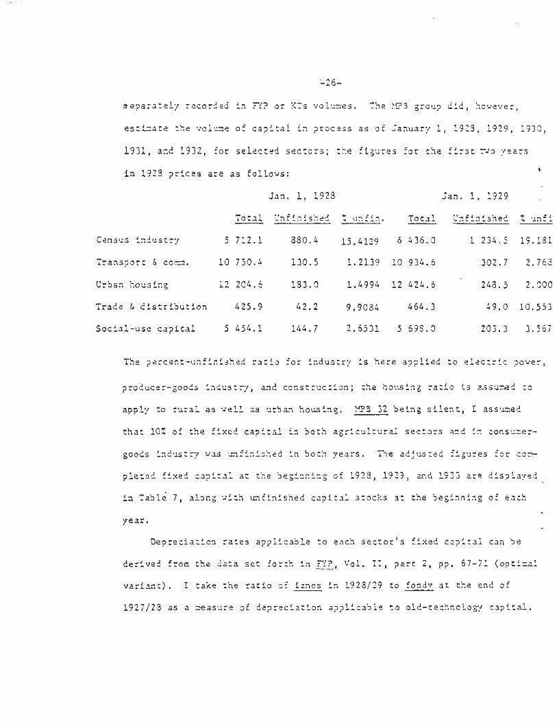
-26-

separately recorded in FYP? or KTs volumes. The MPB group did, however,

estimate the volume of capital in process as of January 1, 1928, 1929, 1930,

1931, and 1932, for selected sectors; Che figures for the first two years

in 1923 prices are as follows:

Jan. 1, 1923 Jan. 1, 1929

Total Unfinished % unfin. Total Unfinished %unfi

Census industry 5 712.1 880.4 15.4129 6 436.0 1 234.5 19.181

Transport & comm. 10 750.4 130.5 1.2139 10 934.6 302.7 2.763

Urban housing 12 204.6 183.0 1.4994 12 424.6 243.5 2.000

Trade & distribution 425.9 42.2 9.9084 464.3 49.0 10.553

Social-use capital 5 454.1 144.7 2.6531 5 698.0 203.3 3.567

The percent-unfinished ratio for industry is here applied to electric power,

producer-goods industry, and construction; the housing ratio is assumed to

apply to rural as ve i l as urban housing. MPB 32 being s i l en t , I assumed

that 10% of the fixed capital in both agricultural sectors and in consumer-

goods industry was unfinished in both years. The adjusted figures for com-

pleted fixed capital at the beginning of 1928, 1929, and 1933 are displayed

in Table 7, along with unfinished capital stocks at the beginning of each

year.

Depreciation rates applicable to each sector 's fixed capital can be

derived from the data set forth in FYP?, Vol. I I , part 2, pp. 67-71 (optimal

variant) . I take the ratio of iznos in 1923/29 to fondy at the end of

1927/23 as a treasure of depreciation applicable Co old-technology capital .

-27-

and the similar ratio for 1932/33 as a measure of depreciation rates appli-

cable to new-technology capital, without attempting an incremental computa-

tion. The sectoral rates are as follows:

Table 7, Adjusted stocks of completed and unfinished capital at the startof 1928, 1929, and 1933, by sector, in millions of rubies at1925/26 prices.

Completed fixed capital Unfinished capital

Population and labor force

Population and labor force estimates for the 1928-1940 period can be

constructed on the foundation of the 1926 Soviet population census, published

in substantial detail by 1929. The potential labor force was necessarily

related to the population aged 16-59; annual changes would reflect the entrance

-28-

of 16-year-olds and the exit of 60-year-olds. The first FYP reviewed many

details of labor force composition, focusing especially on the urban labor

force earning wages and salaries, and projecting changes in the role of the

proletariat vis-a-vis the bourgeoisie. 3ut for the KAPROST model, which

allocates labor to producing sectors as part of each solution, we can confine

ourselves to a measure of the potential labor force available in each year,

along with parameters controlling its allocation and specifying the resulting

earned incomes.

We begin, therefore, with Table 8, which shows estimates of the number

of people (males plus females) reaching age 16 and reaching age 60 for each

year from 1928 through 1941. In the absence of direct intercensal evidence,

these projections come from reported one-year cohorts in the 1926 census,

neglecting the normal mortality that would have thinned the ranks of each age

group after 1926, and thus exaggerating somewhat the labor force increments

hypothetically available. The unadjusted series is taken from the 1926 census

as transcribed in Frank Lorimer, The Population of the Soviet Union (Geneva:

League of Nations, 1946), pp. 231-32. Adjustments are required to smooth out

the pronounced bulges occurring at ages 12, 45, 50, and 55 as people mis-

report their ages. Careful smoothing for the young males was carried out by

Godfrey Baldwin of the Foreign Demographic Analysis Division of the U.S. Dept.

of Commerce in his Estimates and Projections of the Population of the USSR

(series P-91, No. 23, March 1973), p. 10, and I have merely applied his

corrective ratios to the male-female total. The corrections for those aged

45, 50, and 55 in 1926 are cruder. The peak year is assigned a figure repre-

senting the arithmetic mean of the five years centered on it; 352 of the

excess is transferred to the years immediately preceding and following the

-29-

Table 8.

Year ofbirth

191213141516

191718192021

1922232425

Projectedby year,

Age16 in

192829302132

193334353637

1938394041

additions to1928-1941, in

Unadjusted

3 6183 6664 2372 6692 901

2 3223 3353 0133 0583 543

3 6544 5434 4154 527

and subtractions fromthousands

Adjusted

3 6583 7253 7003 3032 976

2 8032 7452 8753 0543 373

3 9204.5334 4154 527

of persons.

Year ofbirth

186869707172

187374757677

1878798081

the population

Unadjusted

699659890

1 548630

750919568

2 175746

1 147952

1 0941 969

aged 16-5

Ad justed

699757

1 118895859

8481 079940

1 1111 118

1 3071 0461 3151 338

peak year; and 152 of the excess is assigned to the adjacent years. Chart 1, p. 30

shows that the smoothed results do not suppress all variation but do display

a more likely pattern than the unadjusted figures. Starting with a base-

period figure for the population aged 16-59 on April 1, 1928 (as set forth

in FYP, Vol. II, part 2, p. 164), we can add those entering at age 16 and

subtract those reaching 60 to bring forward an annual series to 1941.

The first FYP itself contains estimates of the population aged 16-59

from April 1, 1928 through April 1, 1933, together with estimates for the

engaged labor force (FYP, Vol. II, Part 2, p. 164). They imply the annual

increments set forth below, appreciably smaller than those derived above in

Table 8. It will be seen that Gosplan expected the ratio of engaged labor

to population aged 16-59 to rise from 63.06% to 67.76% by 1933.

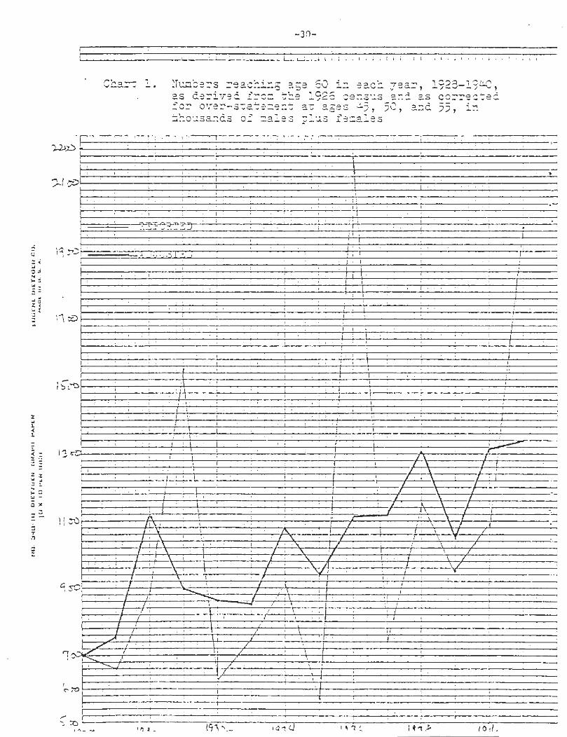
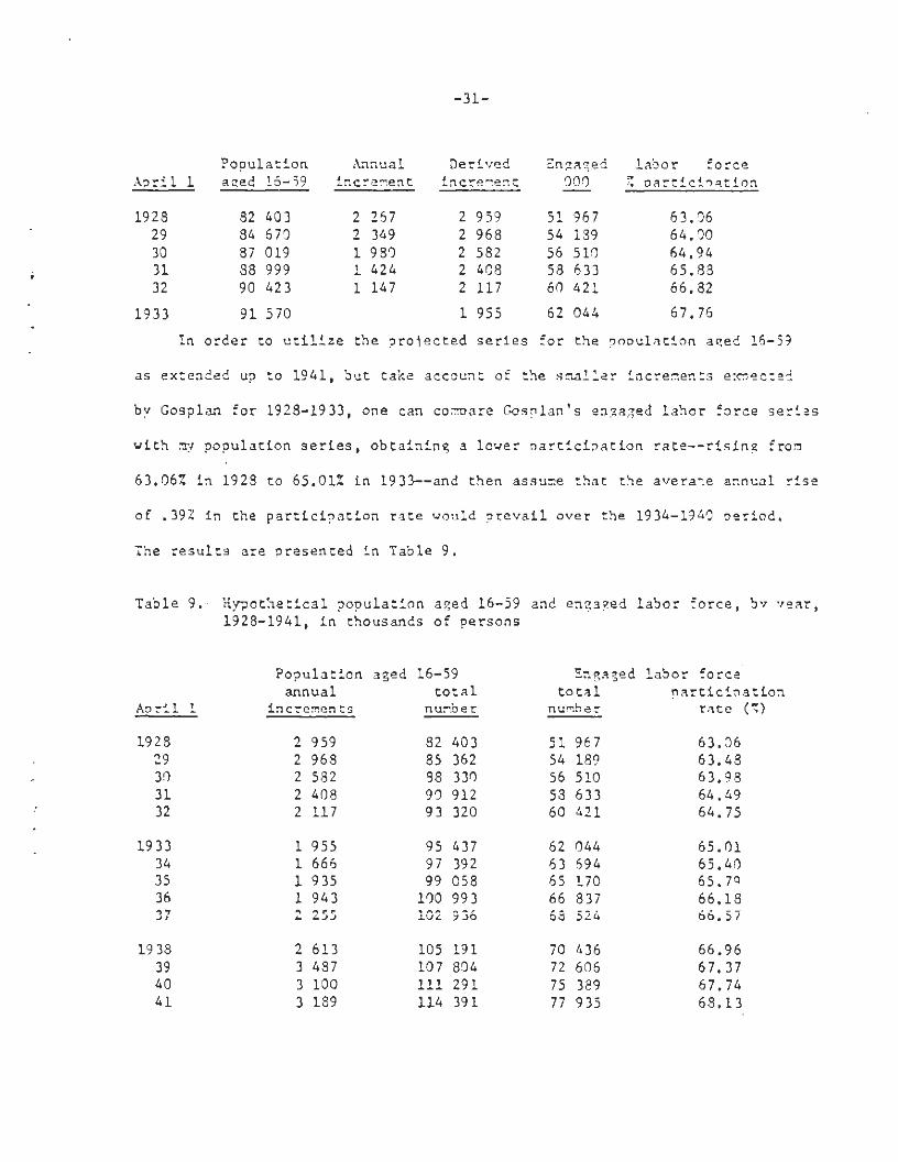
April 1

192829303132

Population.aged 16-59

82 40384 67087 01988 99990 423

Annualincrement

2 2672 3491 9801 4241 147

Derivedincrement

2 9592 9682 5822 4082 117

Engaged000

51 96754 18956 51053 63360 421

labor force% participation

63.0664.0064.9465.8366.32

1933 91 570 1 955 62 044 67,76

In order to util ize the projected series for the population aged 16-59

as extended up to 1941, but take account of the smaller increments expected

by Gosplan for 1928-1933, one can compare Gosplan's engaged labor force series

with my population series, obtaining a lover participation rate—rising from

63.06% in 1928 to 65.01% in 1933—and then assure that the average annual rise

of .39% in the participation rate would prevail over the 1934-1940 period.

The results are presented in Table 9.

Table 9. Hypothetical population aged 16-59 and engaged labor force, by year,1928-1941, in thousands of persons

April 1

Population aged 16-59annual total

increments number

Engaged labor forcetotal participation

number rate (%)

- 3 2 -

The scattered data on employment and wages in plan documents raise many

problems of interpretation and coverage but suffice to provide estimates that

seen adequate for present purposes. Sectoral data on annual wages and employ-

ment, actual for 1923 and intended for 1933, appear in FYP, Vol. I I , part 2,

especially on pages 206 and 208, but also on pp, 9, 13, 16-17, and 48. Besides

the hired labor force employed in state enterprises, other nonagricultural

labor earned incomes in private and cooperative enterprises or as individuals.

The massive and intr icate problem of estimating and projecting earnings and

employment In agriculture is very sketchily dealt with in the first FYP.

The wage and employment figures assembled below are firmest for producer

goods and consumer goods industry, for transport and communications, for trade

and distribution, and for government services. The electric power annual wage

is put at 150% of the 1928 censes-industry wage, on the basis of the relation

shown for 1929 in TsUNKhU, Narkhoz 19 32, p. 460; 192 8 employment Is taken from

Ibid. , p. 422. Employment planned for 1933 is derived from the intended out-

put and an assumed improvement in output-per-man of 110%, comparable to the

highest expected in other high priority branches (FYP?, Vol. I I , part 2, p. 192).

The construction sector used both hired and "other" labor; I have had to

assume that the annual wage for "other" labor was the same as that in ag r i cu l -

ture and forestry. In the absence of any attention to the labor employed in

operating urban residential faci l i t ies or their annual earnings, I have placed

in this sector the servants and day laborers appearing in Gosplan tabulations.

The total nonagricultural wage b i l l in 1928 in Table 10 comes to 9,367

rubles, not very different from the 9, 107 million rubles estimated for urban

incomes by Gosplan (PT?, Vol. I I , Part 2, pp, 72-73). Gosplan's estimates

for workers outlays in this balance of incomes and outlays are clearlv in

purchasers prices, and are incomplete regarding nonhired labor. If non-hired

-33-

Table 10. Annual wage, labor force, and wage bill, by sector, 1928 and 1933,in rubles at 1926/27 prices.

Sector

Agri., field cropsAgri., livestock productsElectric powerProducer goods industryConsumer goods industry

Transport & communicationsConstructionHousingTrade and distributionGovernment services

labor outlays were proportionate to those of hired labor, the 1928 worker con-

sumption total would be 8, 646 million. Deducting excise taxes of 1,396 million

yields a workers consumption estimate in producers prices of 7,250 million rubles,

not drastically different from my flow-table compilation of 6,769 million.

The tota l nonagricultural wage b i l l in 1933 in Table 10 comes to 18,138

million rubles, substantially above my flow-table estimate of 11,99 7 million

of workers consumption outlays in producer:prices. The indicated Gosplan figure

for outlays in purchasers prices is 14,145 million which, when excise taxes of

2,245 million are deducted leaves 11,900 million as an estimate with comparable

coverage.

Agricultural incomes are considerably less certain. The FYP estimates of

agricultural incomes and outlays (FYP, Vol. I I , oart 2, pp, 74-75), include

the following items: 1928 1933

246Gross saving 880

Less: Money credit 19 5

Statistical discrepancy 7

Net saving

Taxes

44

545

41723

440

940

1923

8 533

9 122

.9354

6 769

9 367

.7226

1933

13 729

15 109

.9087

11 997

18 138

..6614

- 3 4 -

I have therefore added 589 million rubles to my compiled flow-cable estimate

for 1928 peasant consumption to obtain an estimate for aggregate 1928 agricul-

tural incomes, and similarly added 1,330 million to the 1933 flow-table peasant

consumption total to get 1933 agricultural income. The indicated "propensities

to consume " are:

Peasants: Consumption

Income

C/Y

Workers Consumption

Income

C/Y

There is little basis in plan documents for subdividing aggregate agri-

cultural income between field crop activities and the production of livestock

products. The rural population earned incomes in many diverse activities and

in fact I have had to ignore the fact that a good deal of their income came

from seasonal jobs in construction or industry. The values of the two output

categories combine with the structure of interindustry flows to leave far less

room for value added in livestock products than in field crops. Thus if, in

the absence of any clues, I assume equal per capita earnings In each branch,

and follow the manpower assignment estimates in FYP , Vol. II, part 2, p. 9 ,

the 1928 flow table will show substantial losses in livestock products. Not

having firm support for any such finding I choose instead to divide the

slender nonwage value added equally between the two branches, thus precipitating

the numbers in lines 1 and 2 of Table 10 . The figures for number of people

in each branch are not intended to convey findings growing out of independent

evidence.

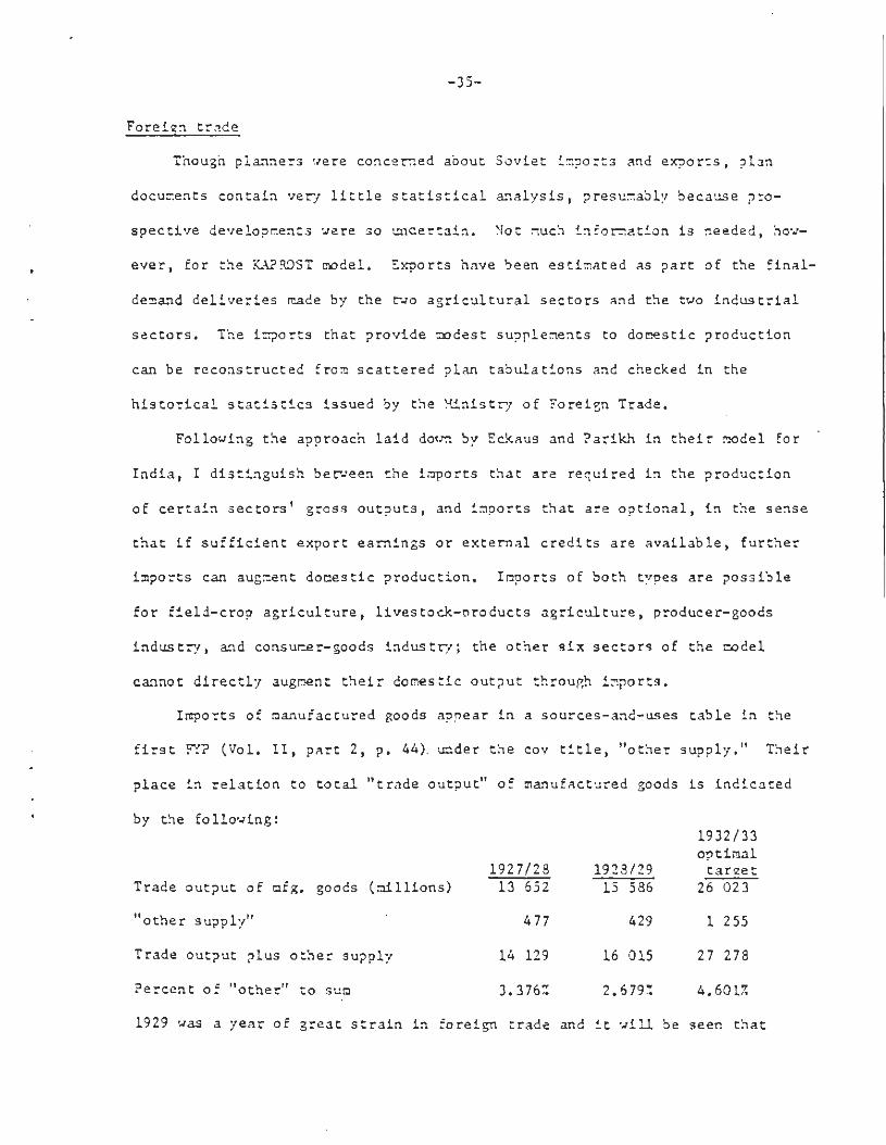
- 3 5 -

Foreign tirade

Though planners were concerned about Soviet imports and exports, plan

documents contain very l i t t l e s tat is t ical analysis, presumably because pro-

spective developments were so uncertain. Not much information is needed, how-

ever, for the KAPROST model. Exrports have been estimated as part of the final-

demand deliveries made by the two agricultural sectors and the two industrial

sectors. The imports that provide modest supplements to domestic production

can be reconstructed from scattered plan tabulations and checked in the

historical stat ist ics issued by the Ministry of Foreign Trade.

Following the approach laid down by Eckaus and Parikh in their model for

India, I distinguish between the imports that are required in the production

of certain sectors' gross outputs, and imports that are optional, in the sense

that if sufficient export earnings or external credits are available, further

imports can augment domestic production. Imports of both types are possible

for field-crop agriculture, livestock-products agriculture, producer-goods

industry, and consumer-goods industry; the other six sectors of the model

cannot directly augment their domestic output through imports.

Imports of manufactured goods appear in a sources-and-uses table in the

first FYP (Vol. I I , part 2, p. 44). under the coy t i t l e , "other supply." Their

place in relation to total "trade output" of manufactured goods is indicated

by the following:

Trade output of mfg. goods (millions)

"other supply"

Trade output plus other supply

Percent of "other" to sum

1929 was a year of great strain in foreign trade and i t will be seen that

1927/2813 652

477

14 129

3.376%

1928/2915 586

429

16 015

2.679%

1932/33optimaltarget

26 023

1 255

27 278

4.601%

-36-

imports fell below the 1923 level though domestic production increased. This

suggests that the 1929 ratio of imports to combined imports-plus-domestic

trade output indicates a minimum of required imports. Applying this ratio to

1928 shows that 378 of the 477 were required and 99 were optional. Applying

the same ratio to 1933 implies that 731 of the 1255 would be required, while

an increased share, namely 524, would be optional under plan intentions.

These estimated amounts may be subdivided between producer goods and consumer

goods on the basis of import data for 1928 in MPB, pp. 187 and 203, providing

shares which are assumed to prevail in 1933 as well. We then have the following

figures, in millions of rubles:

Required Optional Total

Producer goods

1928 Consumer goods

All mfg. goods

Producer goods

1933 Consumer goods

All mfg. goods

Relating these required imports to the flow-table gross outputs, including

interindustry deliveries, yields the following required-import ratios:

Required Imports Gross output Imports/output

1928 producer goods 320 14 676 .02180

1928 consumer goods 58 7 152 .00811

1933 producer goods 619 27 117 .02044

1933 consumer goods 112 13 405 .00836

320

58

378

619

112

731

84

15

99

444

80

524

404

73

477

1063

192

1255

5

5

17

574

259

108

6

6

21

535

402

253

6

6

20

556

349

098

-37-

A similar approach can be used to deduce required and optional imports

of agricultural commodities, though the base-period evidence has to come from

the 1929/30 Congrol Figures (KTs 29/30, pp. 566 and 424-25) and no clues are

available for 1933 plan intentions. A series for "trade output, including

imports, at producers prices" can be compared with another for "trade output

at current prices" (with no mention of imports, and unfortunately for agricul-

tural rather than fiscal years) to precipitate implied imports, as follows, in

millions of rubles:

1927/28 1928/29 1929/30

Including imports

Excluding imports

Gross agri. output, excluding herdgrowth, in current prices

Ratio of imports to gross output .01841 .006256 .01030

The 1928 figure of 315 compares well with a figure of 331 in Min. Vnesh.

Torg., Vneshnaia Torgovlia SSSR za 1928-1940 gg., p. 18. Of this total, some

273 million can be identified therein as involving the following major com-

modities:

Field crops: Cotton 154 Livestock products: wool 61

Vegetables & fruits 9 Large hides 39

Grain 8 Small hides __2

171 102

Applying these proportions to the total of 315 yields the following:

Required Optional Total

1928 field crops 67 130 197

1928 livestock products 40 78 118

Relating these required imports to my flow-table gross outputs produces ratios

of .00609 and .00649, which are assumed unchanged for 1933.

B.1

Appendix 3: Logic and Algebra of the Model

The KAPROST model exists in two forms. The first or structural form

is a familiar set of economic relationships derived from a complete, three-

quadrant input-output system, augmented by production and investment relation-

ships. This version is easy to understand, but contains a very large number of

variables and equations. In order to make the problem more manageable for

computer solution, a second, reduced form of the model was created. It is

derived from the first form by eliminating redundant variables and equations

through substitution. This version is more difficult to understand, but much

less costly to solve.

These aspects of KAPROST are described in three sections. The first

section explains the terminology and symbols used in the model. The second -

and third sections describe structural and reduced forms respectively.

1. Terminology and Symbols

Tables 1 through 4 present concise descriptions of the various terms,

variables and parameters used in the model. The input-output system upon which

KAPROST is based consists of ten productive sectors, listed in Table 1. Both

alphabetic abbreviations and numerical indices are used, the first because

they are easy to remember, the second because they are convenient in specifying

the model equations. The producing sectors may be further grouped as follows.

The agricultural sectors, field crops and livestock, are contrasted with all

other sectors in that our "peasant" and "worker" classification is defined in

of electric power, producer goods, consumer goods, transport and communications,

and, construction. Housing, trade and distribution, and government services

are the service sectors of the economy.

Table 2 relates the periods of the model to historic time. Our pre-

solution base year is 1923, corresponding to period 0. The model is defined

3.2

-28-

Table 1

Sector Names, Abbreviations and Indices

NAME Abbreviation Index

Agriculture-Field Crops

Agriculture-Livestock

Electric Power

Producer Goods

Consumer Goods

Transport and Communications

Construction

Housing

Trade and distribution

Government Services

Throughout the model coding, where an arbitrary sector is to be denoted, we

will use subscripts "i" and " j . "

AF

AL

EP

PG

CG

TC

CO

HO

TD

GS

1

2

3

4

5

6

7

8

9

10

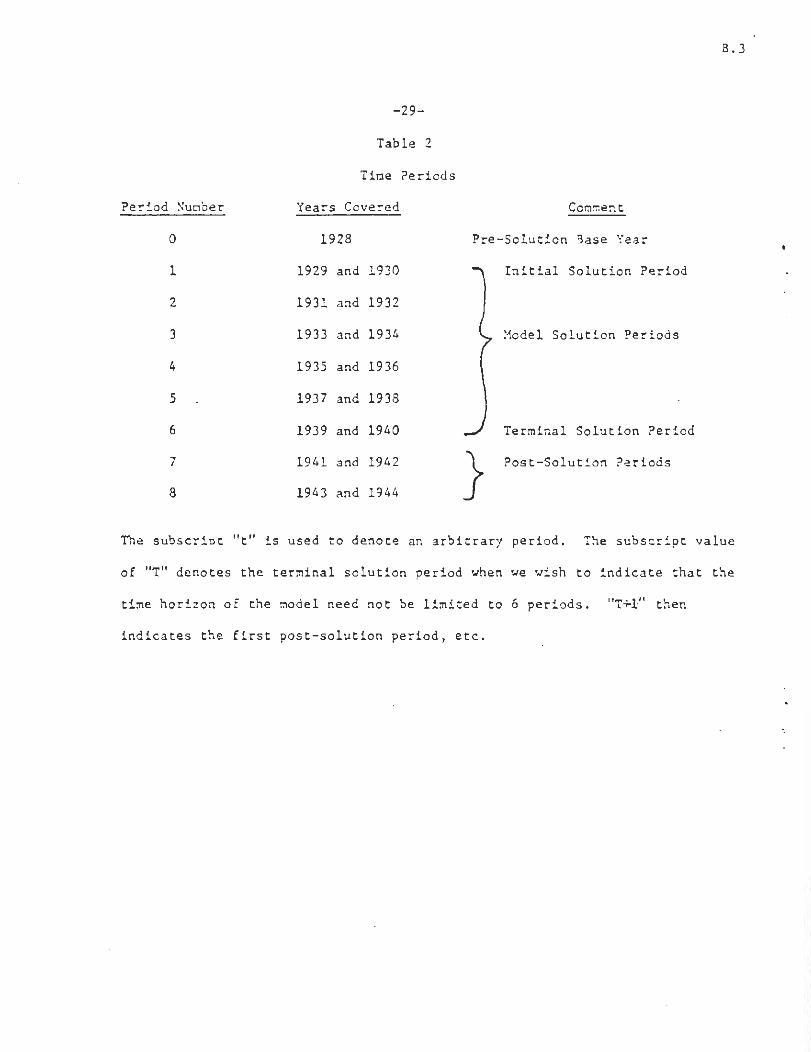
.3

Period Number

0

1

2

3

4

5 .

6

7

8

-29-

Table 2

Time Periods

Years Covered

1928

1929 and 1930

1931 and 1932

1933 and 1934

1935 and 1936

1937 and 1938

1939 and 1940

1941 and 1942

1943 and 1944

Comment

Pre-Solution Base Year

Initial Solution Period

Model Solution Periods

Terminal Solution Period

Post-Solution Periods

The subscript "t" is used to denote an arbitrary period. The subscript value

of "T" denotes the terminal solution period when we wish to indicate that the

time horizon of the model need not be limited to 6 periods. "T+l" then

indicates the first post-solution period, etc.

3.4

in terms of eight periods of two years each, of which the first six are fully

solved for all economic activity. The last two are post-solution periods,

but are of concern to the model in that investment decisions made in the last

two solution periods will affect additions made to capital stock in these post-

solution periods. Note that while our planning horizon is limited to six

periods or twelve years, there is no theoretical reason why this could not be

extended.

The variables used in the model are listed in Table 3 along with a

brief description. Note that all variables have implicit time subscripts and

technology superscripts. Further, some variables require a subscript indi-

cating producing sector, and four of the variables are exogenously specified.

A variable not specified exogenously is solved for by the linear programming

algorithm.

Table 4 describes the parameter and coefficient names, and their

appropriate sub-and superscripting. All of the values for these items are

specified exogenously, though the manner of their derivation differs. Most

parameters are derived from Soviet economic data as described in appendices

A and C. Some, however, are more appropriately considered control parameters,

in that their value is reset by the modeler in order to alter the character-

istics of the solution. The peasant and worker average propensities to consume

(CX., A ) , the post-terminal growth parameters (^), the social discount rate

(r) and the fractions of peasant and worker consumption which must be satisfied

in fixed proportions (D ,j^ ) are control rather than economically derived

parameters.

2. Structural Form of the KAPROST Model

The structural form of the KAPROST model equations are given in Table 5,

and our discussion below refers to the equation numbers used there.

3.5

-30-

Table 3

Glossary of Variable Names

Name

A

CP

cw

D

E

F

G

H

J

K

Description

Foreign Trade Credits (+) or Debits (-)

Total Peasant Consumption

Total Worker Consumption

Amortization Expenditure (Depreciation)

Exports

Consumption

Government Expenditures

Deliveries to Inventory

Inter-Industry Uses

Capital Stock

KAPIPOT Value of the Objective Function

L Labor Force in Use (Required)

M Imports (Required)

N Deliveries to Fixed Capital

0C Optional Consumption0M Optional/Discretionary Imports

S Available Labor Force

X Gross Output

YP Peasant Income

YW Worker Income

Z Additions to Capital Stock

Varies bySector ! Period

exogenousVariable

X

X

X

X

X

X

X

X

X

X

X

X

X

x

X

X

X

X

X

X

XX

X

X

X

X

X

X

X

X

X

X

A variable which varies by sector will have its sector index as its firstsubscript; the time period index will always be the last subscript.Thus "X " is the gross output of sector "l" in period "t"

Note the inter-industry flow variable, J, requires two sector indices; thefirst for the producing sector, the second for the consuming sector.

3.6

-31-

Thus "J " is the delivery of output from industry "i" to industryijt

" j " in period "t."

A superscript indicates type of technology: "0" for old, "N" for new.

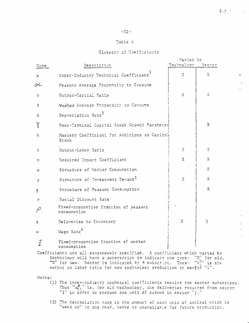
Name

a

-32-

Table 4

Glossary of Coefficients

Description

Inter-Industry Technical Coefficient

Peasant Average Propensity to Consume

Output-Capital Ratio

Worker Average Propensity to Consume

Depreciation Rate2

Varied byTechnology Sector

Post-Terminal Capital Stock Growth Parameter

Mastery Coefficient for Additions to CapitalStock

Output-Labor Ratio

Required Import Coefficienti

Structure of Worker Consumption

Structure of Investment Demand"3

Structure of Peasant Consumption

Social Discount RateFixed-proportion fraction of peasantconsumption

Deliveries to Inventory

Wage Rate

Fixed-proportion fraction of workerconsumption

Coefficients are all exogenously specified. A coefficient which varied bytechnology will have a superscript to indicate the type: "0" for old,"N" for new. Sector is indicated by a subscript. Thus: "XN" is theoutput to labor ratio for new technology production in sector "i".

Notes :(1) The inter-industry technical coefficients require two sector subscripts.

Thus lvaP^ ' is, for old technology, the deliveries required from sector"I" in order to produce one unit of output in sector " j . "

(2) The depreciation rate is the amount of each unit of capital which is"used up" in one year, hence is unavailable for future production..

3.8

-33-

Table 4 (cont'd.)

(3) Investment in capital follows a rigid, two-period (r year) schedule.

Thus "P " is the initial period deliveries to fixed capital from

sector "i" to eventually yield one unit of new capital in sectorVT

" j " , and "P* " is the second period deliveries.

(4) Wage rate varies by sector and by period. "W " is the wage paid

labor in sector "I" in period "t."

B.9

-34-

Table 5

Structural Equations

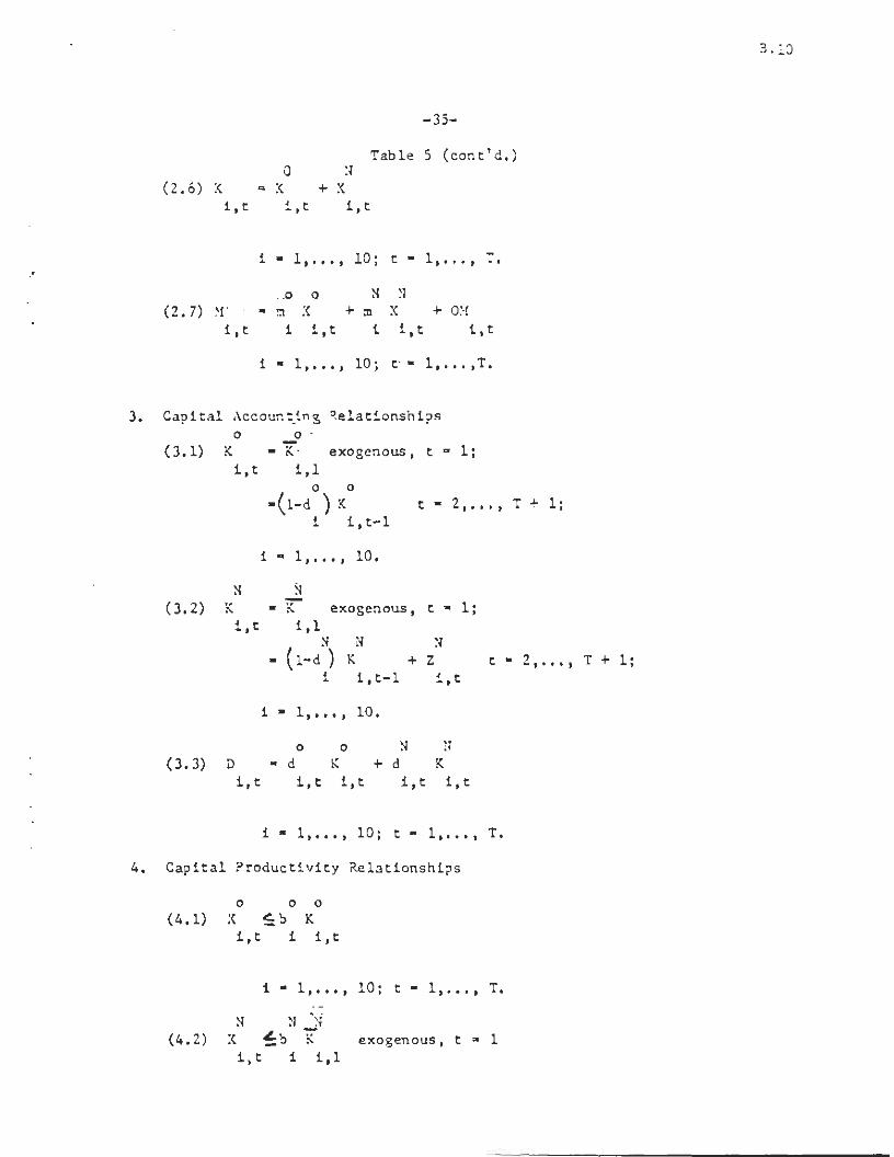
B.10

-35-

Table 5 (cont'd.)

4. Capital Productivity Relationships

3.11

- 3 6 -

Table 5 ( c o n t ' d . )

7. Balance of Payments Relationship

3.12

-37-

Table 5 (cont'd.)

8. Terminal Investment Requirement

B.13

A linear programming model is an optimizing model, and so requires an

objective function. Equation 1.0 presents an objective function which contains

peasant and worker consumption in each year, and new technology capital stock

in the first post-terminal year. The initial weighting scheme sets all weights

for the year 1940 to 1, and raises the weight on consumption in earlier years

by an appropriate power of the social discount rate in order to compensate for

the passage of time. Clearly these basic weights are only a starting point for

analysis, and in the course of simulation the coefficients on ail items in the

objective were changed in order to alter the characteristic of the solution.

Note that the objective function captures the primary dilemma of development:

the time pattern of consumption, investment and capital formation by sector.

The distribution relationships are composed of the row identity of

input-output system (2.1) which limits the sum of the uses of any sector in any

period to the sum of gross output and imports of that sector in chat period.

Equation (2.2) defines interindustry demand as a result of the gross output of

each sector times the appropriate technical coefficient, for old and new

technology production. Equation (2.3) shows the dependence of deliveries to

fixed capital on the increments to capital stock in the next two periods.

Capital requires a two period (four year) gestation period in KAPROST, with

coefficients for the investment which must occur in each of the two periods in

order for capital stock to increase.

Exports and government spending are exogenously specified. Equation

(2.4) shows the three components of consumption: the fractions of peasant and

worker consumption which must be satisfied in fixed proportions and optional

consumption. Our Soviet data shows a fairly stable pattern of actual 1928 con-

sumption and planned consumption in the first five year plan. We interpret this

as representing consumer preference and require part of the consumption demand

of peasants and workers to be satisfied according to the fixed proportions of

3.14

these patterns. The rest of their consumption may be optionally filled from

any sector at the discretion of the solution algorithm.

Production requires some level of inventories, and in equation (2.5)

deliveries to inventory are given as a fixed fraction of output. Similarly in

equation (2.6) imports required for production are given as a fixed fraction of

output, and total imports by sector and period are the sum of these and optional

imports. Note that required inventory and import levels vary by the producing

technology. Equation (2.6) indicates that gross output is the sum of that

produced under old and new technology.

The capital accounting relationships record the effects on initial

levels of capital stock of depreciation and new increments. Equation (3.1) an

(3.2) are for old technology and new technology capital respectively, with the

only difference in treatment due to our limiting investment to new technology

production. Equations (3.3) calculates total depreciation.

Production is limited to a fixed multiple of capital stock as indicated

in equations (4.1) and (4.2). The complexity of the relation for new technology

production results from the requirement that increments to capital stock are not

fully productive in the year they are made. Rather, only the fraction k of

additions to capital, plus the undepreciated fraction of the previous period's

capital stock are available for production. This specification is intended to

represent the lower productivity which occurs while new capital is mastered by

the labor forced, or worked in to use.

KAPROST uses the output-labor ratios to determine the required labor

force for the output produced in each sector (equations (5.1) and (5.2), subject

to the constraint of total labor force (equation (5.3)). Note that one result

of this specification is that unemployment, a phenomenon never observed in the

Soviet Union, is possible. Rather than interpreting unrequired workers as

3.1

unemployed, it is probably more accurate to consider them as supernumeraries

in their place of work..

Income is a result of wages to required labor, as given in equations

(6.1) and (6.2). Note that wages do not vary by technology. Equations (6.3)

and (6.4) express, for peasants and workers, the requirement that total con-

sumption be at least a given fraction of total income. These fractions may be

viewed as average propensities to consume, or as inflation factors relating

nominal income to real wage in consumption goods. In equation (6.5) we require

total consumption to be satisfied in part by a fraction which must be delivered

in fixed proportions of output from the producing sectors, and in part by

optional consumption delivered from any sector.

Equation (7.1) requires that the foreign trade accounts for each year

be in balance or in surplus.

Finally, the terminal investment requirement (equation (8.1)) forces

deliveries to investment in the last solution period be high enough to allow

additions to capital stock in the second post-terminal period to exceed average

additions over the model solution period, plus some fraction of the final capital

stock.

Note that each equation in Table 5 is simply a template. They must be

expanded into separate equations either for each sector or for each time period

or for every combination of sector and time period in order to completely

specify the model.

3. Reduced Form of the KAPROST Model

The reduced fora of the KAPROST model is presented in Table 6. It is

obtained by substituting the equalities of the structural form into the in-

equalities so as to eliminate redundant variables. Here we indicate the sub-

stitutions made.

B.16

Table 6

Reduced Form Equations

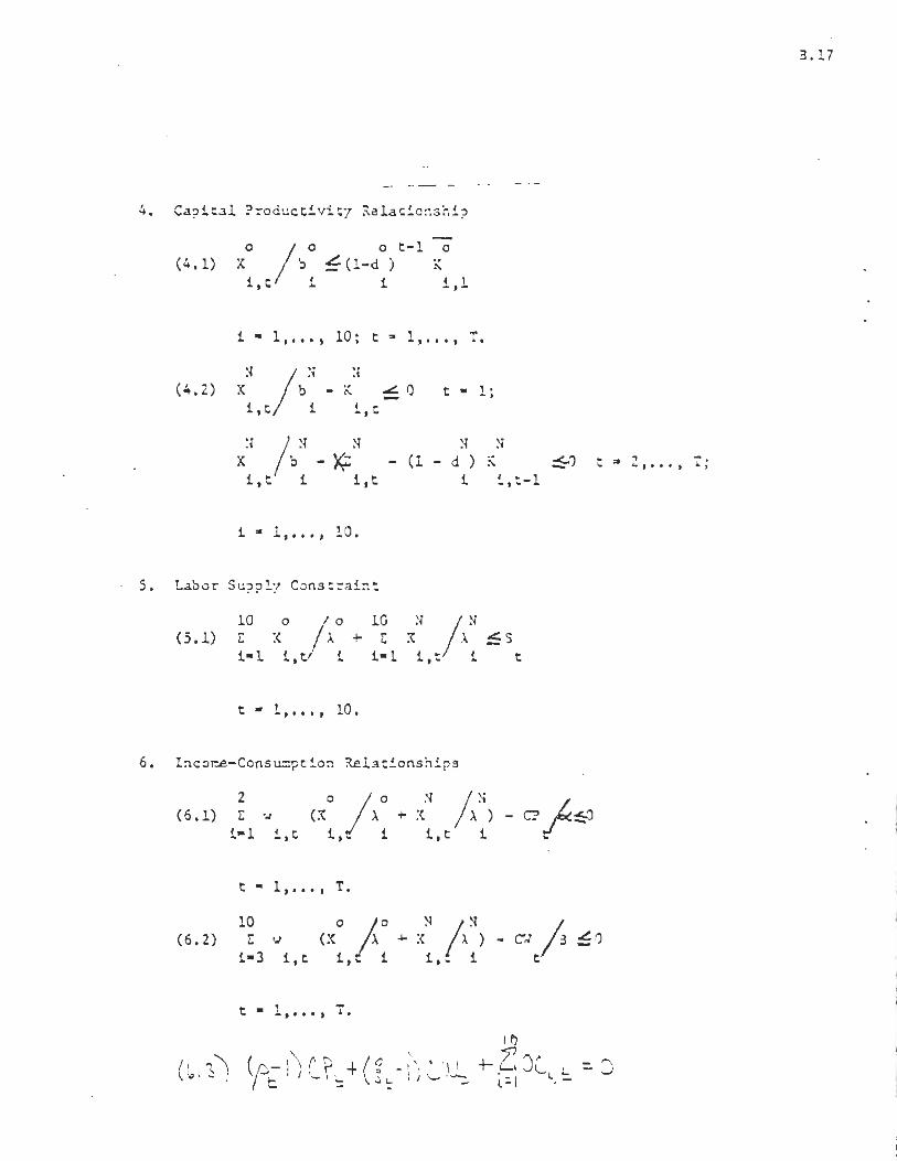
B.17

B.18

B.19

The objective function, equation (1.0) remains unchanged. The new

distribution relationship (2.1) is obtained by substituting the definitions

of each of the components of the input-output table row constraint into that

constraint, grouping common factors, and isolating all exogenous variables on

the right hand side. This last step normalizes the form of the problem for

the linear programming solution algorithm, and is done for all of the equations

below.

The capital accounting relationships (equations (3.1) and (3.2) repeat

the time progress of new technology capital as it appears in Table 5, making

explicit the exogenous setting of the initial period new technology capital stock,

and second period additions to new technology capital stock.

Accounting relationships for old technology capital stock may be disposed

of; no investment in old technology capital is permitted, the exogenously

specified initial value simply depreciates so that the stock for each year is

effectively exogenous. This is most evident in the productivity relationship

for old technology capital (equation (4.1)) where output from old technology

is limited by the remainder of the initial stock after the appropriate number

of years of depreciation. The relation for new technology in equation (4.2) ,

notes the effect of the mastering requirement for additions to capital. Note

that all variables in equations (4.2) appear on the left hand side as they are

all solved for by the model.

The labor supply constraint given in equation (5.1) is obtained by

substituting output divided by the output to labor ratio for labor. This sub-

stitution is also made in the income-consumption relationships (6.1) and (6.2)

to calculate income and then relate it to consumption by the average propensities

to consume. The requirement that total consumption be properly divided between

a part received in fixed proportions and an optional portion is normalized in

equation (6.3).

3.20

The balance of payments constraint in equation (7.1) shows the substi-

tution of the definition of required imports into the structural form in Table

5. The terminal investment constraint (equation (8.1)) has simply been

normalized.

As with the structural form equations in Table 5, the reduced form

equations in Table 6 are only templates. They must be expanded for all

appropriate sectors and time periods in order to yield a complete linear

programming problem.

C.I

Appendix C: Data as Modified for Use by the

KAPROST Model

The data estimates from Soviet and other sources presented in

Appendix A need to be reformulated in order to correspond with the KAPROST

model described in appendix B. These calculations, the motivating assumptions,

and the data used are described here. Note that this appendix presents the

data values which correspond exactly to the problem free solution. While most

of these values also underlie the historic simulations, the reader should be

aware of the distinction. The alternatives used for specific historic simula-

tions are described in the body of the report with the simulation results.

1, Exports

Soviet sources provide historic export levels for 1923, and those

forecast for 1933 by the first five year plan. The problem free solution is

assumed to provide these forecast amounts, and for years between 1928 and 1933,

and after 1933, amounts given by linear interpolation and extrapolation. Table 1

gives the yearly values so obtained. As the KAPROST time periods are two years

each, these values are summed appropriately to yield the exports for each of

the six solution periods of the model (Table 2). Note that only the agricultural,

(both field crops and livestock),producer goods and consumer goods sectors par-

ticipate in foreign trade.

2. Government Expenditures

The development of government expenditures is affected by our use of a

government services producing sector, which delivers output only to the govern-

ment. Our intention in doing this was to have all normal government expenditures

reflected in demand for the output of the government services sector, which

required interindustry deliveries from other producing sectors, and associated

that output with requirements for labor and capital stock. This provides,

C.2

Year

Table 1

Exports (millions of rubles)

Industry

AF AL PG CG

1928192919301931193219331934193519361937193819391940

7684.492.8

101.2109.6118126.4134.8143.2151.6160.0168.4176.8

230258.8287.6316.4345.2374402.8431.6460.4489.2518546.8575.6

263370.6478.2585.8693.4801908.6

1016.21123.81231.413391446.61554.2

50 -62748698110122134146158170182194

The 1928 values are actual exports; the 1933 values are those projectedby the first five year plan. All others are the result of linearinterpolation or extrapolation from the 1928 and 1933 figures.

AF: Agriculture, Field Crops

AL: Agriculture, Livestock

PG: Producer Goods

CG: Consumer Goods

C.3

Period

Table 2

Exports by KAPROST Period(millions of rubles)

AF

Industry

AL ?G CG

1929 and 1930

1931 and 1932

1933 and 1934

1935 and 1936

1937 and 1933

1939 and 1940

177.2

210.8

244.4

278.0

311.6

345.2

546.4

661.6

776.8

892.0

100 7.2

1122.4

843.3

1279.2

1709.6

2140.0

2570.4

3000.3

136

184

232

280

328

376

Values reflect two year totals from Table 1.

AT: Agriculture, Field Crops

AL: Agriculture, Livestock

PG: Producer Goods

CG: Consumer Goods

These numbers provide values for the variable "E" in KAPROST for sectors1 , 2, 4 and 5. Exports of all other sectors are zero.

C.4

again for normal government activity, a neat way of combining deliveries from

other sectors, labor force and productive capital stock, rather than associate

these with a final demand category directly. For other than normal scenarios,

e.g. rearmament, government demand for producers goods can be specified directly,

as tanks, planes, ships, etc., are produced by this sector yet do not enter

into capital stock, but are considered to be consumed. However, the labor force,

barracks, and common needs of soldiers can be provided for by increasing

government expenditure on the output of government services, as this increases

demands on all these items in proportion, plus forcing additional wage payments

and consumption demands to round out the non-heavy goods requirements of the

military.

For the problem free solution we again took actual 192S and projected

1933 government expenditures and obtained values for intervening and succeeding

years by linear interpolation and extrapolation. These were summed over two

year intervals to obtain the G10 variable in KAPROST. Direct government

expenditures on the output of all other sectors is zero. These results are

presented in table 3.

3. Labor Supply

Yearly labor force statistics must be converted to values appropriate

to KAPROST's two-year periods. This is done by taking the average labor force

over the two years, and is presented in table 4.

4. Initial Levels of Capital Stock

The basic data for capital stock consist of actual 1928 and 1929 levels,

plus an indication of additions to capital stock based on projects in progress

in 1928. These last provide direct estimates for Zl» additions to new tech-

nology capital in the second period, as given in table 5. We must therefore

c. 5

disentangle the 1923 and 1929 stock figures to provide estimates of initial

period capital stock of both technologies.

Our basic assumption is that all capital stock in 1928 is of the old

technology, and no additions are made to it so that the only process affecting

it is depreciation. Hence for each sector, the initial period stock of old

technology capital is equal to the 1923 stock of capital minus depreciation.

The initial period stock of new technology capital is the difference between

the total 1929 stock and the calculated initial stock cf old technology capital

These calculations are reproduced in table 6.

Year

Table 3

Government "Expenditures on Government Services(in mil l ions of rubles)

G10by Year Period G10

1923192919 301931193219331934193519361937193319 391940

2954.03554.84155.64756.25357.25958,06558.87159.67760.48361.28962.09562.3

10163.6

1929

1931

1933

1935

1937

19 39

and

and

and

and

and

and

1930

1932

1934

1936

1938

1940

7710.4

10113.6

12516.8

14920.0

17323.2

19726.4

G10 is the government expenditure on the output of sector 10,government services. Direct government expenditure on theoutput of all other sectors is zero (though indirectly, thproduction of G10 requires output from several sectors).

C6

Year

Table 4

Labor Supply (in thousands)

LaborSupply Period

Labor

1923192919 3019 31193219331934193519361937193319 391940

51967541895651058633604216204463694651706683768524704367260675339

1929

1931

1933

1935

1937

1939

and

and

and

and

and

and

1930

1932

1934

1936

1938

1940

55350

59527

62869

66004

69430

73998

The period labor supply is the average of the yearly labor suppliesin that period.

The last column data provide values for the variable S in KAPROST.

Table 5

Additions to New Technology Capital Stockin Period 2

Sector

(millions of rubles)

N

AFALEPPGCGTCCOHOTDGS

3151140194

1308697"33115947974

213

.7

Table 6

Initial Period Stocks of Capital(millions of rubles)

Sector

(1)

1928CapitalStock

(2)

DepreciationRate

(3)InitialPeriodOldTechnologyCapitalStock

(4)

1929CapitalStock

(5)InitialPeriodNewTechnologyCapitalStock

AFALEPPGCGTCCOHOTDGS

8224759460030172618

11366595

22982487

5680

.087

.0768

.0524

.0517

.0509

.0358

.0994

.039

.0485

.0284

7509701156928612485

10959536

220864635519

84887965817

33852937

11608667

23490627

5765

979954248524452649131

1404164246

Column 1 and 4 are historic values

Column 3 = (1-Column 2) * Column 1

Column 5 = Column 4 - Column 3

Column 3 provides the exogenous values for K_,

Column 5 provides the exogenous values for K?

,1

C.3

5. Depreciation Coefficients

The one-year depreciation rates obtained from Soviet data need to be

converted to the two-year model periods. As the depreciation rate gives the

proportion of each unit of capital used up in one year, one minus this rate

is the proportion remaining after one year. The square of the proportion

remaining after one year is the proportion remaining after two, and the

difference between this and one the two-year depreciation rate. These calcu-

lations are repeated in Table 7.

6. Fixed Proportion Structure of Consumption

The sector proportions in which peasants and workers would choose to

consume, given the opportunity, are based on actual 1923 consumption and planned

1933 consumption. As these proportions did not change significantly over the

five years, the consumption-weighted averages of the two observations were used.

Table 8 presents these calculations.

7. Wages

The actual 1928 wages and planned 1933 wages by sector are used to

linearly interpolate and extrapolate values for the remaining years (Table 9).

These values are summed over two-year intervals to provide the sector wages

for KAPROST (Table 10).

8. Investment Structure

The time pattern of deliveries from capital-goods producing sectors

to investment demand in order to eventually make a new unit of capital available

to a given sector is a combination of two sets of coefficients. Table 11 lists,

for each sector, the proportions of Livestock, Producers Goods and Construction

which go into one ruble of capital stock. It is then assumed that capital

is produced over two, two-year periods, with .2398 of the deliveries occurring

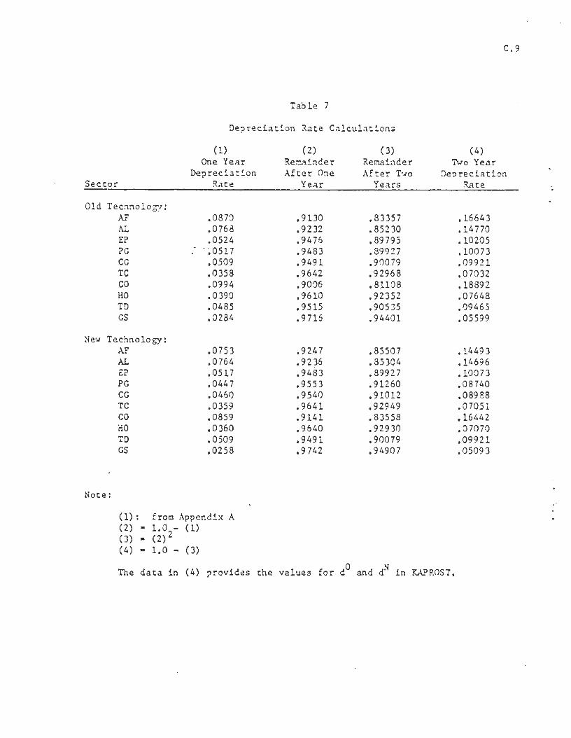
C.9

Table 7

Depreciations Rats Calculations

Sector

Old Technology:AFALEPPGCGTCCOHOTDGS

New Technology:AFALEPPGCGTCCOHOTDGS

(1)One Year

DepreciationRate

.0870

.0768

.0524

.0517

.0509

.0358

.0994

.0390

.0485

.0284

.0753

.0764

.0517

.0447

.0460

.0359

.0859

.0360

.0509

.0258

(2)RemainderAfter One

Year

.9130

.9232

.9476

.9483

.9491

.9642

.9006

.9610

.9515

.9716

.9247

.9236

.9483

.9553

.9540

.9641

.9141

.9640

.9491

.9742

(3)RemainderAfter Two

Years

.83357

.85230

.89795

.89927

.90079

.92968

.81108

.92352

.90535

.94401

.85507

.85304

.89927

.91260

.91012

.92949

.83558

.92930

.90079

.94907

(4)Two Year

DepreciationRate

.16643

.14770

.10205

.10073

.09921

.07032

.18892

.07648

.09465

.05599

.14493

.14696

.10073

.08740

.08988

.07051

.16442

.07070

.09921

.05093

Note:

( 1 ) : from Appendix A(2) = 1.0 - (1)(3) - ( 2 ) 2

(4) - 1.0 - (3)

The data in (4) provides the values for d and <f in KAPROST,

C.10

Table 8

Fixed Consumption Structure

(1)1923

Consumption

(2)1923

Shares

(3)1933

Consumption

(4)1933

Shares

(5)Total

Consumption

(6)AverageShares

Peasants

AFALEP?G.CGTCCOHOTDGS

Total

14002995—34

2003120—8001181—

SS33

.16407

.35099—

.00398

.23474

.01406—

.09375

.13840—

1.00000

22934752—56

3284159—10202165—

13729

.16702

.34613—

.00408

.23920

.01158—

.07430

.15770—

1.00000

36937747—90

5287279—18203346—

22262

.16589

.34799—

.00404

.23749

.01253—

.08175

.15030—

1.00000

AFALEPPGCGTCCOHOTDGS

tal

6361051—59

2149286—8941644—

6769

.10134

.15527—

.00872

.31748

.04225—

.13207

.24287—

1.00000

11191668—93

3414369—15413793—

1199 7

.09327

.13903—

.00775

.28457

.0307.6—

.12345

.31616—

1.00000

18052719—152

5563655—24355437—

13766

.09618

.14489—

.00810

.29644

.03490—

.12976

.29973——

1.00000

Note:(1)(2)(3)(4)(5)(6)

from Soviet 1928 data(1) divided by column totalfrom First Five Year Plan(3) divided by column total(1) + (3)

(5) divided by column total.

Ail calculations performed separately for Peasants and Workersyields values for * and w in KAPROST.

Column 6

flows in mil l ions of rubles.

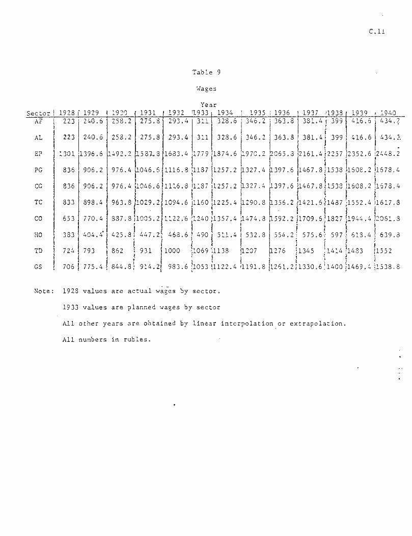
C.11

Table 9

Wages

Note: 1928 values are actual wages by sector.

1933 values are planned wages by sector

All other years are obtained by linear interpolation or extrapolation

All numbers in rubles.

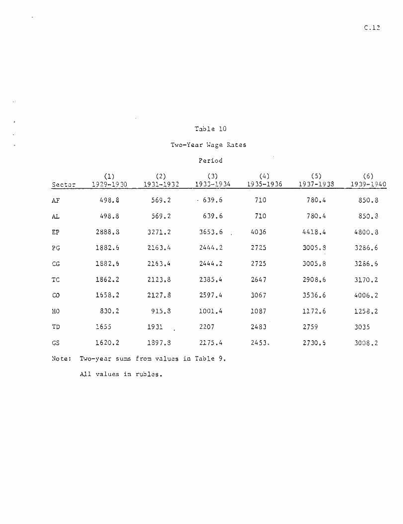
C.12

Sector

AF

AL

EP

?G

CG

TC

CO

HO

TD

GS

Note:

(1)1929-1930

A98.8

498.8

2888.8

1882.6

1882.6

1862.2

1658.2

830.2

1655

1620.2

Two-year sums

(2)1931-1932

569.2

569.2

3271.2

2163.4

2163.4

2123.8

2127.8

915.8

1931

1897.8

Table 10

(3)1933-1934

- 639.6

639.6

3653.6 .

2444.2

2444.2

2385.4

2597.4

1001.4

2207

2175.4

from values in Table 9.

(4)1935-1936

710

710

4036

2725

2725

2647

3067

1087

2483

2453.

(5)1937-1938

780.4

780.4

4418.4

3005.8

3005.8

2908.6

3536.6

1172.6

2759

2730.6

(6)1939-1940

850.8

850.8

4800.8

3286.6

3286.6

3170.2

4006.2

1258.2

3035

3008.2

All values in rubles.

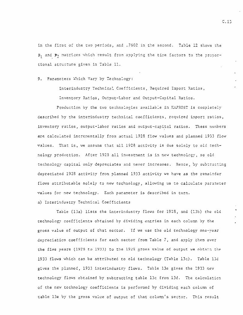
C.13

in the first of the two periods, and .7602 in the second. Table 12 shows the

p1 and p2 matrices which result from applying the time factors to the propor-

tional structure given in Table 11.

9. Parameters Which Vary by Technology:

Interindustry Technical Coefficients, Required Import Ratios,

Inventory Ratios, Output-Labor and Output-Capital Ratios.

Production by the two technologies available in KAPROST is completely

described by the interindustry technical coefficients, required import ratios,

inventory ratios, output-labor ratios and output-capital ratios. These numbers

are calculated incrementally from actual 1928 flow values and planned 1933 flow

values. That is, we assume that all 1928 activity is due solely to old tech-

nology production. After 1928 all investment is in new technology, so old

technology capital only depreciates and never increases. Hence, by subtracting

depreciated 1928 activity from planned 1933 activity we have as the remainder

flows attributable solely to new technology, allowing us to calculate parameter

values for new technology. Each parameter is described in turn.

a) Interindustry Technical Coefficients

Table (13a) lists the interindustry flows for 1928, and (13b) the old

technology coefficients obtained by dividing entries in each column by the

gross value of output of that sector. If we use the old technology one-year

depreciation coefficients for each sector from Table 7, and apply them over

the five years (1928 to 1933) to the 1928 gross value of output we obtain the

1933 flows which can be attributed to old technology (Table 13c). Table 13d

gives the planned, 1933 interindustry flows. Table 13e gives the 1933 new

technology flows obtained by subtracting table 13c from 13d. The calculation

of the new technology coefficients is performed by dividing each column of .

table 13e by the gross value of output of that column's sector. This result

C.14

Table 11

Investment Structure of Capital

SectorReceivingCapital

AF

AL

EP

PG

CG

TC

CO

HO

TD

GS

Capital Goods

AL

.1834

.6562

---

Producing Sector

PG

.5645

.1186

.6676

.4987

.4987

.4477

.7390

.3518

.4786

.1052

CO

.2501

.2252

.3324

.5013

.5013

.5523

.2610

.6842

.5214

.8948

Note: Each entry indicates the ruble value of deliveriesfrom a capital goods producing sector to investmentdemand to produce one ruble of capital in the sectorreceiving new capital.

C.15

SectorReceivingCapital

Table 12

Tine Structure of Capital Production

(1)First Period

(2)Second Period

Capital Producing Sector

AL PG CO

Capital Producing Sector

AL PG CO

AF

AL

EP

PG

CG

TC

CO

HO

TD

GS

.0445 .1354

.1574 .0284

.1601

.1196

.1196

.1074

---- .1772

.0757

.1148

.0252

.0600

.0540

.0797

.1202

.1202

.1324

.0626

.1641

.1250

.2146

.1409 .4291

.4988 .0902

.5075

.3791

.3791

.3403

.5618

.2401

.3638

.0800

.1901

.1712

.2527

.3811

.3811

.4199

.1984

.5201

.3964

.6802

Note: (1) = Table 11 x 0.2398

(2) - Table 11 x 0.7602

Ruble value of deliveries to investment to produce oneunit of capital available at the beginning of the. third period,

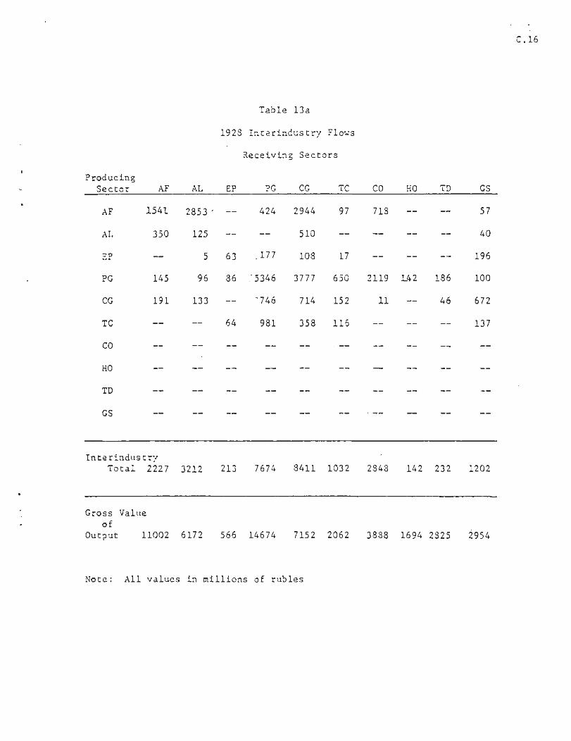
C.16

Table 13a

1928 Interindustry Flows

Receiving Sectors

ProducingSector

AF

AL

EP

PG

CG

TC

CO

HO

TD

GS

AF

154.1

350

—

145

191

—

—

—

—

—

AL

2853 '

125

5

96

133

—

—

—

—

—

EP

—

—

63

86

—

64

—

—

—

—

?G

424

—

.177

."5346

-746

981

—

—

—

—

CG

2944

510

108

3777

714

358

—

—

—

—

TC

97

—

17

650

152

116

—

—

—

CO

718

—

—

2119

11

—

—

—

—

- —

KO

—

—

—

142

—

—

—

—

—

—

TD

—

—

—

186

46

—

—

—

—

—

GS

57

40

196

100

672

137

—

—

—

—

InterindustryTotal 2227 3212 213 7674 8411 1032 2848 142 232 1202

Gross Valueof

Output 11002 6172 566 14674 7152 2062 3888 1694 2825 2954

Note: All values in millions of rubles

C.17

Table 13b

Old Technology Coefficients

Receiving Sectors

ProducingSectors

AF

AL

EP

PG

CG

TC

CO

HO

TD

GS

AF

.14007

.03181.

—

.01318

.01736

—

—

—

—

AL

.46225

.02025

.00081

.01555

.02155

—

—

—

—

EP

—

—

.11131

.15194

—

.11307

—

—

—

PG

.02889

—

.01206

.36432

.05084

.06685

—

—

—

.....

CG

.41163

.07131

.01510

.52810

.09983

.05006

—

—

—

TC

.04704

— ,

.00824

.31523

.07371

.05626

—

—

—

CO HO

.18467

—

—

.54501 .08383

.00283

—

—

—

—

__ __

TD

—

—

—

.06584

.01628

—

—

—

—

__

GS

.01930

.01354

.06635

.03385

.22749

.04638

—

—

—

Note: Obtained from table 13a by dividing each column by its gross value ofoutput.

0Provides a values in KAPROST.

. 10

Table 13c

Old Technology Flows in 1933

Receiving Sectors

Note: Obtained by depreciating table 13a overfive years. Rounded to nearest unit.Values in millions of rubles.

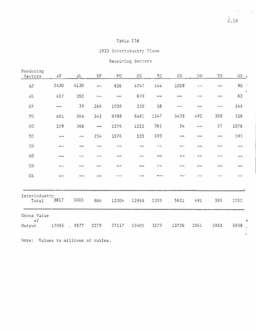
C.19

ProducingSectors

AF

AL

EP

?G

CG

TC

AF

2430

457

—

401

529

AL

4130

202

39

266

368

1933

EP

—

—

269

343

—

254

Table 13d

Interindustry F

Receiving

?G

626

—

1038

8788

1276

1576

lows

Sectors

CG

4747

670

330

6461

1222

535

TC

144

—

58

1547

361

193

CO

1059

—

—

5438

24

HO

—

—

—

492

—

__

TD

—

—

—

308

77

__

GS

90

62

545

326

1076

193

CO

HO

TD

GS

InterindustryTotal 3817 5005 866 13304 13965 2303 5621 492 385 2292

Gross Valueof

Output 17065 . 9577 2279 27117 13405 3279 13726 2561 5958 5958

Note: Values in millions of rubles.

C.20

Table 13e

New Technology Flows in 19 33

Receiving Sectors

InterindustryTotal 2404 2851 703 7419 7487 1442 3935 376 204 1250

Gross Value

of Output . 10086 5438 . 1847 15864 7897 1561 11423 1173 3755 3400

Note: (13e) = (13d) - (13c)

Values in millions of rubles.

C.21

is presented as table 13f.

b) Required Import Ratios

Table 14 lists the incremental calculations Co obtain the required

import ratios for old and new technology production.

c) Inventory Ratiosv

Table 15 lists the incremental calculations to obtain the inventory

ratios for old and new technology production.

d) Output-Labor Rat ios

The old technology output-labor ratios are obtained by dividing 1923

gross values of output by sector labor force. This is multiplied by two to obtain

productivity over the two-year KAPROST period. 1933 old technology labor force

equals 1933 old technology gross value of output multiplied by the one-year old

technology output-labor ratios. This is subtracted from total 1933 labor force.

We use this as the divisor for 1933 new technology gross value of output to

obtain new technology output-labor ratios. Again, multiplication by two adapts

the data to the two-year period of KAPROST. See Table 16.

e) Output-Capital Ratios

Table 17 shows the calculation of old and new technology output-capital

ratios. As this exactly parallels the calculation of the output-labor ratios

discussed above, no further concent is warranted.

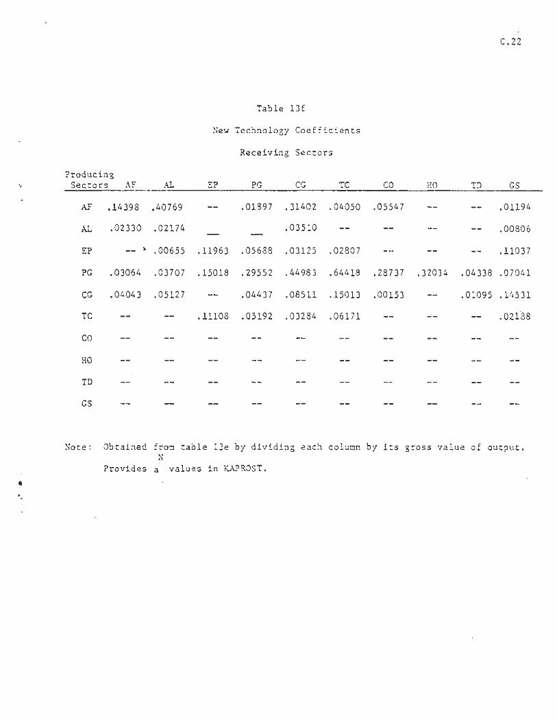
C.22

ProducingSectors

AF .:

AL

EP

PG

CG

TC

CO

HO

TD

GS

AF

L4398

02330

03064

04043

—

—

—

—

AL

.40769

.02174

.00655

.03707

.05127

—

—

—

—

New

EP

—

.11963

.15018

—

.11108

—

—

—

Table

Technology

Receiving

PG

.01897 .

.05688 .

.29552 .

.04437 .

.05192 .

—

—

—

13f

Coefficients

Sectors

CG

31402

03510

03125

44983

08511

03284

—

—

—

TC

.04050

—

.02807

.64418

.15013

.06171

—

—

—

CO

.05547

—

---

.28737

.00153

—

—

—

—

HO TD

—

—

—

.32034 .04338

.01095

—

—

—

—

GS

.01194

.00806

.11037

.07041

.14531

.02188

—

—

—

Note: Obtained from table 13e by dividing each column by its gross value of output.N

Provides a values in KAPROST.

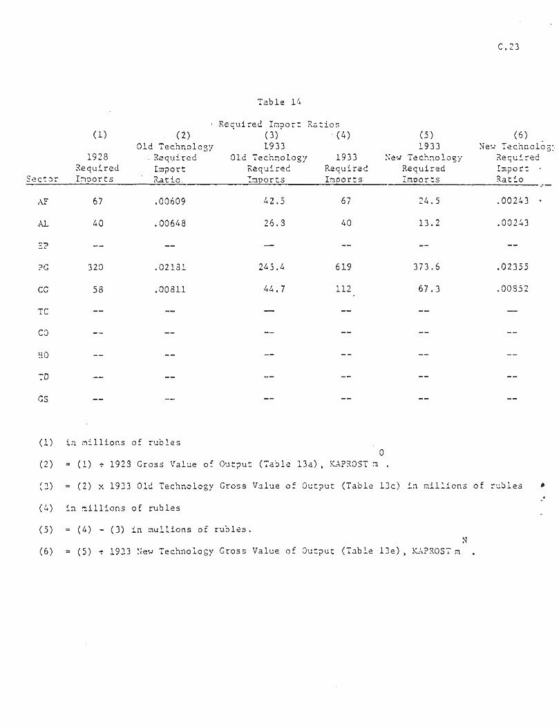
C.23

Table 14

• Required Import Ratios(1) - (2) (3)' (4)

Old Technology 1933Old Technology 1933

Required RequiredImports Importsctor

AF

AL

EP

?G

CG

TC

CO

HO

TD

GS

1928RequiredImports

67

40

—

320

58

—

—

—

—

. RequirImportRatio.

.00609

.00648

—

.02181

.00811

—

—

—

—

--

(5)1933

New TechnologyRequiredImports

(6)New Technology

RequiredImportRatio

42.5

26.8

245.4

44.7

67

40

619

112

24.5

13.2

373.6

67.3

.00243

.00243

.02355

.00852

(1) in millions of rubles0

(2) = (1) ÷ 1928 Gross Value of Output (Table 13a) , KAPROST m .

(3) = (2) x 1933 Old Technology Gross Value of Output (Table 13c) in millions of rubles

(4) in millions of rubles

(5) = (4) - (3) in millions of rubles.N

(6) = (5) ÷ 1933 New Technology Gross Value of Output (Table 13e) , KAPROST m .

C.24

Table 15

Inventory Ratios

(1) (2) (3) (4) (5) (6)Old 1933 Old 1933 New New

1928 Technology Technology 1933 Technology TechnologyDeliveries to Inventory Deliveries to Deliveries to Deliveries to Inventory

Sector Inventor' Ratios Inventory Inventory Inventory Ratios

AF

AL

EP

?G

CG

TC

CO

HO

TC

GS

206

—

—

30

234

—

515

—

—

.01872

—

—

.00545

.03272

—

.13246

—

—

__

130.6

—

—

61.3

180.2

—

305.1

—

—

__

309

—

—

350

1564

—

1819

—

—

178.3

—

—

288.7

1383.8

—

1513.9

—

—

.01768

—

—

.01820

.17523

—

.13253

—

—

(1) in millions of rubles0

(2) = (1) ÷ 1928 Gross Value of Output (Table 13a) , KAPROST s

(3) = (2) x 1933 Old Technology Gross Value of Output (Table 13c) in millions of rubles.

(4) in millions of rubles

(5) = (4) - (3) in millions of rubles

(6) = (5) ÷ 1933 New Technology Gross Value of Output (Table 13e) in millions of rubles,KAPROST sN

C.24

Table 16

Output-Labor Ratios

sect0

r

A?

AL

EP

?G

CG

TC

CO

HO

TD

GS

(1)

1928LaborForce

34770

3810

19

1767

3894

1410

1255

754

1065

2215

(2)One-Year

OldTechnology

Output-LaborRatio

.31642

1.61995

29.78947

8.30447

1.83667

1.46241

3.09801

2.24668

2.65258

1.33363

(3)Two-Year

OldTechnologyOutput-LaborRatio

.63284

3.23990

59.57895

16.60894

3.67334

2.92482

6.19602

4.49337

5.30516

2.66727

(4)

1933Old

TechnologyLaborForce

22058

2555

15

1355

2999

1175

744

618

831

1918

(5)

1933LaborForce

41310

4700

36

2754

4767

1545

209 7

868

1357

2754

(6)

1933New

TechnologyLaborForce

19252

2145

22

1399

1768

370

1354

250

526

836

(7)One—Year

NewTechnology

Output-LaborRatio

.52386

2.53532

85.95789

11.34034

4.46612

4.21836

8.43960

4.69041

7.13280

4.06658

(8)Two-Year

New;

TechnologyOutput-Labor'Ratio

1.04771

5.07063

171.91578

22.68068

8.93225

8.43672

16.37920

9.38082

14.26560

8.13315

(1) in thousands

(2) = 1928 Old Technology Gross Value of Output (Table 13a)* (1).

(3) 2.0 x (2) , KAPROST Xc

(4) = (2) x 1933 Old Technology Gross Value of Output

(Table 13c) in thousands

(5) in thousands

(6) = (5) - (4)

(7) - 1933 New Technology Gross Value of Output (TAble 13e)

(8) - 2.0 x (7) , KAPROST \n

* (6)

C.25

Table 17

Output-Capital Ratios

sector

AF

AL

EP

PG

CG

TC

CO

HO

TD

GS

(1)

1928Capital

Stock

8224

7594

600

3017

2618

11366

595

22982

487

5680

(2)One-Year

OldTechnologyOutput-CapitalRatio

1.338

.813

.94333

4.86377

2.73186

.18142

6.53445

.07371

5.80082

.52007

(3)Two-Year

OldTechnologyOutput-CapitalRatio

2.676

1.625

1.88666

9.72754

5.46371

.36284

13.06891

.14742

11.60164

1.04014

(4) (5)

1933Old

Technology 1933 .Capital CapitalStock Stock

5217

5093

458

2314

2016

9472

353

18837

380

2558

11600

10151

3191

9754

4867

18273

2100

28507

2318

10088

(6)

. 1933New

TechnologyCapitalStock

6383

5058

2733

7440

2851

8801

1748

9670

19 38

7530

(7)One-Year

NewTechnologyOutput-CapitalRatio

1.580

1.075

.67563

2.13217

2.76991

.17732

6.53677

.12125

1,93746

.45157

(8)Two-Year

NewTechnologyOutput-Capital

Ratio

3.160

2.150

1.35126

4.26434

5.53981

.35464

13.07353

.24250

3.87492

.90313

D.1

Appendix D: Programming and Computer Solution of the Model

The model described in Appendix 3 is an optimization model with linear

objective function and linear constraints, that is, it is a linear programming

model. We chose to use the IBM Mathematical Programming System (MPS) to

solve the model, both for reasons of availability and because it is one of the

most common linear programming packages in use. Our model was solved success-

fully by MPS on on IBM 360 Model 44 with 256 K of main storage. For a

detailed description of MPS please refer to the IBM publications listed at the

end of this appendix.

Use of MPS requires that all of the linear relations be formatted in

the MPS input language. A glance at the reduced form of the model (Appendix B,

Table 6) shows that the form of most relations is very regular, with entries

varying by industrial sector, time period or both. Further, even with the

economies in the reduced form description, the model still has over 300 con-

straints and over 600 variables, which would require a considerable amount of

keypunching to produce input acceptable to MPS. If this task were performed

only once, the direct keypunch approach would be feasible. However, our research

task required that we be able to vary parameter values quite often, and re-keying

changes would have been intolerable.

The regularity of the model, therefore, proved to be a blessing in

disguise, because it permitted us to write computer program which would accept

the parameters of the model as data, and then automatically generate the

appropriate input to MPS. This preliminary processing program, or PREL, was

written in the PL/I programming language, a choice dictated by the need for

character manipulation capabilities. PREL is highly idiosyncratic in that it

produces MPS input for only one model, KAPR0ST. For that reason we do not

describe it in detail (though a copy can be provided on request). However,

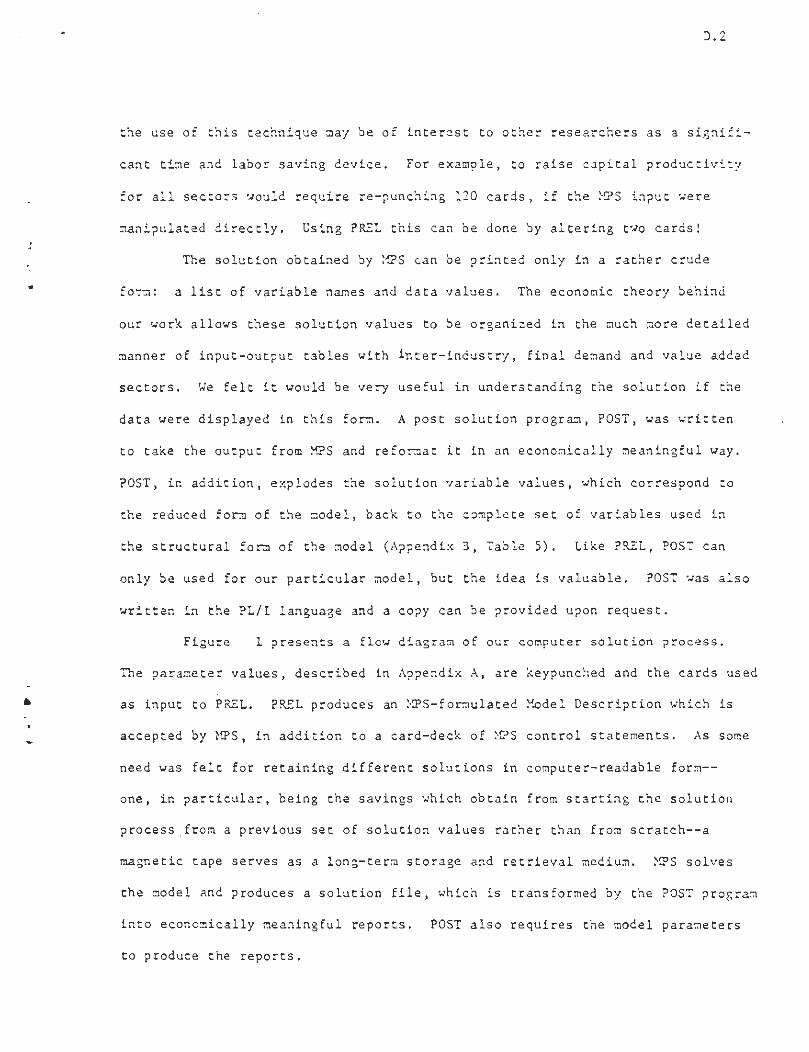
D.2

the use of this technique may be of interest to other researchers as a signifi-

cant time and labor saving device. For example, to raise capital productivity

for all sectors would require re-punching 120 cards, if the M?S input were

manipulated directly. Using PREL this can be done by altering two cards!

The solution obtained by MPS can be printed only in a rather crude

form: a list of variable names and data values. The economic theory behind

our work allows these solution values to be organized in the much more detailed

manner of input-output tables with inter-industry, final demand and value added

sectors. We felt it would be very useful in understanding the solution if the

data were displayed in this form. A post solution program, POST, was written

to take the output from MPS and reformat it in an economically meaningful way.

POST, in addition, explodes the solution variable values, which correspond to

the reduced form of the model, back to the complete set of variables used in

the structural form of the model (Appendix 3, Table 5). Like PREL, POST can

only be used for our particular model, but the idea is valuable. POST was also

written in the PL/I language and a copy can be provided upon request.

Figure 1 presents a flow diagram of our computer solution process.

The parameter values, described in Appendix A, are keypunched and the cards used

as input to PREL. PREL produces an MPS-formulated Model Description which is

accepted by MPS, in addition to a card-deck of MPS control statements. As some

need was felt for retaining different solutions in computer-readable form—

one, in particular, being the savings which obtain from starting the solution

process from a previous set of solution values rather than from scratch—a

magnetic tape serves as a long-term storage and retrieval medium. MPS solves

the model and produces a solution file, which is transformed by the POST program

into economically meaningful reports. POST also requires the model parameters

to produce the reports.