Testing for Altruism and Social Pressure in Charitable Giving∗

Stefano DellaVigna

UC Berkeley and NBER

John A. List

U Chicago and NBER

Ulrike Malmendier

UC Berkeley and NBER

This version: December 22, 2009.

(First version: May 2009)

Abstract

Every year, 90 percent of Americans give money to charities. Is such generosity necessar-

ily welfare enhancing for the giver? We present a theoretical framework that distinguishes

two types of motivation: individuals like to give, e.g., due to altruism or warm glow, and

individuals would rather not give but dislike saying no, e.g., due to social pressure. We

design a door-to-door fund-raising drive in which some households are informed about the

exact time of solicitation with a flyer on their door-knobs; thus, they can seek or avoid the

fund-raiser. We find that the flyer reduces the share of households opening the door by 10

to 25 percent and, if the flyer allows checking a ‘Do Not Disturb’ box, reduces giving by

30 percent. The latter decrease is concentrated among donations smaller than $10. These

findings suggest that social pressure is an important determinant of door-to-door giving.

Combining data from this and a complementary field experiment, we structurally estimate

the model. The estimated social pressure cost of saying no to a solicitor is $3.5 for an

in-state charity and $1.4 for an out-of-state charity. Our welfare calculations suggest that

our door-to-door fund-raising campaigns on average lower utility of the potential donors.

∗We thank Saurabh Bhargava, David Card, Constanca Esteves-Sorenson, Bryan Graham, Lawrence Katz,Patrick Kline, Stephan Meier, Klaus Schmidt, Daniel Sturm and the audiences at the Chicago Booth School

of Business, Columbia University, Harvard Business School, University of Arizona, UC Berkeley, UT Dallas,

University of Zurich, the 2009 San Francisco Applied Micro Conference, the 2009 Conference in Behavioral

Economics, the Munich Workshop on “Natural Experiments and Controlled Field Studies”, and the ASSA 2009

Meetings for helpful comments. We also thank Daniel Acland, Diane Alexander, Jim Cai, Matthew Levy, Xiaoyu

Xia, and especially Gautam Rao for excellent research assistance.

1 Introduction

In the U.S. alone, annual individual giving to charity exceeds 2 percent of GDP, with approxi-

mately 90% of people donating money. There is at least one capital campaign to raise $25 mil-

lion or more under way in virtually every major population center in North America. Smaller

capital campaigns are even more numerous, with phoneathons, door-to-door drives, and mail

solicitations increasing in popularity. While the stakes are clearly quite high, many economic

facts concerning the interrelationship between solicitors and solicitees remain unknown. De-

spite a substantial literature on charitable giving (see, e.g., the overview by Andreoni, 2006),

we still have an imperfect understanding about the motivations for different forms of giving.

In this paper, we consider two broad classes of motivations. First, individuals may give

because they enjoy giving. For example, they may care about a specific worthy cause or like

the warm glow of giving. Second, individuals may give despite not liking to give to the charity

because the solicitor effectively placed them under social pressure to give. Such givers would

rather have avoided the personal interaction with the solicitor, had they only been warned.

The two views have very different welfare implications. The altruism (or warm glow) model

(Fehr and Gaechter, 2000; Andreoni, 1989 and 1990) posits that giving is mostly supply-driven,

and that it is utility-maximizing for the giver to give. Under this model, the above transaction

increases the giver’s utility and represents an overall enhancement of societal welfare. The

social pressure model (Akerlof and Kranton, 2000) posits that giving is mostly demand-driven,

and that giving may be utility-reducing for the giver.

We test for these two types of motivations in the context of personal, unsolicited donation

requests. Building on a theoretical model, we design and implement a field experiment in an

actual marketplace for charitable giving. The model and the experimental design allow us to

distinguish whether giving is welfare-enhancing or welfare-reducing for the giver. Using the

reduced-form experimental evidence, we estimate the parameters of the model structurally.

This allows us to quantitatively evaluate the welfare effects for the giver and to decompose the

share of giving that is due to altruism versus social pressure. In this way, the empirics and

theory are intertwined in a manner that is rare in this literature.

Our field experiment revolves around a door-to-door fund-raising drive for two charities, a

local children’s hospital, which has a reputation as being a premier hospital for children, and

an out-of-state charity, that most solicitees are unaware of. We approached 7,668 households

in the towns surrounding Chicago in the period between April and October 2008. We view this

field experiment as just a first step towards better understanding the underpinnings for giving

more generally. While the door-to-door set-up is specific, it showcases a general methodology.

The crucial aspect of our experimental design is to allow individuals to sort, i.e., to either

seek or avoid the solicitor. In our first treatment, a flyer on the doorknob notifies households

one day in advance about the one-hour time interval in which a solicitor will arrive at their

1

home the next day. In the second treatment, ‘Opt-out’, the flyer also includes a box that can be

checked if the household does ‘not want to be disturbed’. We compare these two conditions to

a baseline treatment, wherein our solicitors approach households in the usual manner without

a flyer. We estimate the impact of the treatments on both the share of households that answer

the door and on the share of households that give.

This design allows for a simple test of the importance of (pure or impure) altruism and of

social pressure. If altruism is the main driver of giving, the flyer should increase both presence

at home and giving. Since giving is utility-enhancing, households should sort into staying at

home, provided alternative ways of giving to these charities require more effort. In addition,

households who intend to give in response to the flyer but who find it too costly to be at

home should give to the charity via other means. Conversely, if social pressure is the main

driver of giving, the flyer should lower both presence at home and giving. Since being asked to

give is welfare-diminishing, households should sort out of opening the door. In addition, the

households that are not at home during the visit of the solicitor will not give via other means,

such as mailing a check, since these forms of donation are not subject to social pressure.

We report four main reduced-form results. First, the flyer treatments lower the frequency of

opening the door substantially: relative to a baseline rate of 41 percentage points in the baseline

treatment, the share of households opening the door is 10 percent lower in the Flyer condition

and 25 percent lower in the Opt-Out condition. The effect is similar for both charities.

Second, the mere presence of a flyer on the door-knob has no effect on actual giving: 6.3

percent of all households give in both the baseline and the Flyer treatment. However, if the

flyer includes an opt-out checkbox, giving decreases by 30 percent relative to the baseline

group. The treatment effect is again similar for both charities, though the level of giving is

higher for the local charity in all conditions.

Third, the decrease in giving in the Opt-Out treatment is driven by small donations up to

$10. Donations above $10, instead, increase slightly (not significantly) in the treatments with

sorting relative to the baseline treatment.

Fourth, there is no effect on donations via mail or Internet. In contrast to the substantial

donation rates in person, only one contacted household out of 7,668 gave through these other

means.

Overall, our reduced form estimates indicate that both altruism and social pressure are

important determinants of giving in this setting, with stronger evidence for the role of social

pressure. The lower frequency of households opening the door to a solicitor after receiving a

flyer indicates that households are on average trying to avoid the solicitors, consistent with

social pressure. The lack of an effect of the baseline flyer on giving is consistent with opposing

effects of altruism and social pressure approximately cancelling each other out. The decrease

in giving after a flyer with opt-out box supports the role of social pressure: When the cost to

avoid the solicitor is lowered (a simple check on a box suffices), giving due to social pressure

2

decreases. This interpretation is consistent with the reduction occurring almost exclusively

among small donations, which are more likely due to social pressure than large donations. The

social pressure interpretation is also consistent with the lack of donations via mail or Internet.

To address the welfare effects of giving, we complement the reduced-form estimates with a

structural estimation of the parameters in the model. We combine data from the experimental

treatments discussed above with data from complementary field experiments on the value of

time run in the same areas in 2008 and 2009. In these experiments, we ask households to

complete a survey. We vary whether the surveys are announced (with a flyer, with or without

opt-out option), the payment ($0, $5, or $10), and the duration (5 or 10 minutes) of the survey.

We find that increased payment and shorter duration increase the presence at home by 5 to

15 percent. These same treatments significantly increase the share willing to undertake the

survey by 20 to 80 percent. The responsiveness with respect to a monetary incentive provide

information to identify the underlying parameters structurally.

We use a minimum-distance estimator on the combined data from the charity and the

survey experiments. The estimator minimizes the distance between the moments predicted by

the model and the observed moments. The moments are the probabilities of opening the door,

of giving different amounts, of completing a survey, and of opting out. Key parameters are the

mean and variance of the altruism distribution and the social pressure cost—the cost of saying

‘no’ in person to a solicitor. We estimate that on average potential donors are not altruistic,

but that 10 to 15 percent prefer to give a positive amount. The estimated social pressure cost

is $3.5 for the highly-liked, in-state charity and $1.4 (not significantly different from zero) for

the out-of-state charity.

We use the parameter estimates to decompose the observed giving and to compute welfare

effects for the baseline fund-raiser (without flyer). We estimate that 70 to 80 percent of donors

would have given even in absence of social pressure. However, a substantial share of these

donors gives more (due to social pressure) than they would have liked too. As a result, half of

donors derive negative utility from the fund-raising interaction, and would have preferred to

sort out. Still, the remaining half of givers derive positive warm-glow or altruism out of giving.

Given the large social pressure costs on all the non-givers, the door-to-door solicitations

in our sample lower utility of the households solicited on average. For the in-state charity,

a visit is estimated to lower welfare by $1.04, and to raise on net only about $0.35, for each

household contacted. If we take our fund-raising campaigns to be representative of door-to-door

solicitation, unsolicited campaigns lead to utility losses for the givers equivalent to hundreds

of millions of dollars.1

These results have implications for the optimal taxation regime of charitable giving. The

tax advantaged status of charitable giving has its roots in the assumption that giving increases

1The campaigns, of course, may still be welfare improving overall if the charities spend the money very

effectively.

3

societal welfare including, presumably, the welfare of the giver. This assumption is largely

untested. We provide evidence that welfare-decreasing motives to give are at least as important

in door-to-door solicitations as welfare-increasing motives. This suggests that tax subsidies may

be designed to provide a separate consideration for high social-pressure forms of giving, such

as door-to-door and phone giving.

These findings can also be used as an argument to introduce a do-not-solicit or do-not-call

list for charities. However, they also suggest a simple alternative: providing households with the

opportunity to sort or, even better, to opt out. Introducing sorting opportunities in fund-raising

limits, or eliminates altogether, the welfare losses for the solicitees. Interestingly, introducing

sorting can also increase charitable fund-raising, and be a win-win solution: even a limited

amount of sorting in of altruistic givers, who give larger amounts, is likely to counterbalance

the sorting out of givers motivated by social pressure, who give smaller amounts.

A methodological contribution of this paper is the close tie between a behavioral model and

a field experiment, allowing for structural estimation of the underlying parameters. Among

the behavioral field experiments (surveyed in Harrison and List, 2004 and DellaVigna, 2009),

we are only aware of Bellemare and Shearer (2009) which estimates a model of reciprocity

using data from a gift exchange field experiment. In other fields, Duflo, Hanna, and Ryan

(2009) among others combine field experiments and structural estimation. A small number

of behavioral papers structurally estimate models on observational data, including Laibson,

Repetto, and Tobacman (2007) and Conlin, O’Donoghue, and Vogelsang (2007).

Beyond its methodological contribution, our paper adds to several literatures. First, it

provides field evidence of behaviors that have been found to be important in laboratory exper-

iments (Fehr and Gachter, 2000, Charness and Rabin 2002, Dana, Weber, and Kuang, 2007).

Most closely related to this paper, a recent laboratory literature examines the impact of allow-

ing subjects to sort out of the giving situation and finds that this leads to a substantial decrease

in transfers (Dana, Caylain, and Dawes, 2006; Lazear, Malmendier, and Weber, 2009). We also

find a decrease in giving in response to sorting, but only when costs are lowered sufficiently

through an opt-out option.

Second, it complements the literature that explores optimal fund-raising approaches using

field experiments (e.g., List and Lucking-Reiley, 2002; Landry et al., 2006; Croson and Shang,

2009; Fong and Luttmer, 2009; Ariely, Bracha, and Meier, 2009), as well as to a theoretical

literature on the reasons for giving (see, e.g., Andreoni, 2004). The tighter link between the

model and the experimental design in our paper will hopefully help bridge the gap between

the theoretical and the empirical literature.

Third, it builds on a literature in psychology (Asch, 1951 and Milgram, 1963), in economics

(Garicano, Palacios-Huerta, and Prendergast, 2005; Falk and Ichino, 2006; Mas and Moretti,

2009), and in political science (Gerber, Green, and Larimer, 2008) on the effect of social

pressure. Our model of social pressure is a reduced-form representation of utility-diminishing

4

models of giving, whether social pressure, social norms (Bernheim, 1994), or self- and other-

signaling (Bodner and Prelec, 2002; Benabou and Tirole, 2006; Grossman, 2007). In this

respect, the evidence from the Opt-Out treatment suggests that self- and other-signaling is

unlikely to explain door-to-door giving, since checking a do-not-disturb box is presumably a

strong signal of unwillingness to give.

The rest of the paper proceeds as follows. In Section 2 we present a simple model of giving

with altruism and social pressure. We introduce the experimental design in Section 3 and

discuss the reduced-form results of the treatments in Section 4. In Section 5, we structurally

estimate the underlying parameters of the model, and in Section 6 we conclude.

2 Model

We model an individual’s response to a solicitor who visits a home and asks for a donation.

We distinguish between the standard case of an unanticipated visit and an anticipated visit

(household received a flyer). In the latter case, the giver can alter the probability of being

at home and opening the door to the solicitor. If the flyer has a do-not-disturb option, the

adjustment is costless; otherwise, it is costly.

Setup. We consider a two-stage game between a potential giver and a solicitor. For

convenience, we denote the potential giver, or solicitee, simply as ‘giver.’

In the first stage, the giver does or does not receive a notice of the upcoming visit of the

solicitor (flyer). The giver notices the flyer with probability r, with 0 < r ≤ 1. If she does notnotice the flyer (or does not receive one), she is at home and opens the door with probability

h0, with 0 < h0 < 1. If she notices the flyer, she chooses a probability h of being at home and

opening the door in the second stage, with 0 ≤ h ≤ 1. To adjust this probability from the

baseline h0 to h, she incurs a cost c (h), with c(h0) = 0, c0(h0) = 0, and c00(·) > 0. That is,

there is no cost of being at home with the baseline probability h0, and the marginal cost of

small adjustments is small, but larger adjustments have an increasingly large cost. We do not

require symmetry around h0 and we allow for corner solutions at h = 0 or h = 1.

In the second stage, the solicitor visits the home. With probability h, the giver is present

and donates an amount g ≥ 0. With probability 1− h, she is absent, in which case there is no

in-person donation (g = 0). The giver can donate an amount gm through other channels, such

as via mail or online, after learning about the charity from the solicitor or the flyer.

The giver has utility

U (g, gm) = u (W − g − gm) + av (g + θgm, G−i)− s (g) . (1)

Private consumption is the pre-giving wealthW minus the donation given to the solicitor g and

donations given through other channels gm. The private utility satisfies standard monotonicity

and concavity properties: u0(·) > 0 and u00(·) ≤ 0. The utility of giving in person to the

5

charity v can depend on the giving of others G−i and satisfies similar assumptions: v0g(·, ·) > 0,v00g,g(·, ·) < 0, and limg→∞ v0 (g, ·) = 0. We assume v(·) ≥ 0, that is, the utility of giving inperson is non-negative, and normalize the utility of no giving to zero: v(0, G−i) = 0. The utilityof giving via mail is a scaled-down version of the utility of giving in person, v (θgm,G−i) , with0 ≤ θ < 1. The assumption θ < 1 captures the costs to giving via mail, such as finding an

envelope and stamp, as well as the possibility that giving through an impersonal mean such

as mail yields lower utility.2

Expression (1) allows for both the case of pure altruism (Charness and Rabin 2002, Fehr

and Gachter, 2000) and impure altruism (warm glow, Andreoni, 2004). In the case of pure

altruism, the agent cares about the total contributions to the charity G−i+g+θgm, which are

used to provide a public good through a production function v (G−i + g + θgm) . This yields

utility av (G−i + g + θgm), where the parameter a captures the level of altruism, which can be

negative if the giver dislikes the charity. In the case of impure altruism, the agent cares about

the warm glow associated with giving g, implying that the utility v (·) does not necessarilydepend on the giving of others G−i. In this case, the parameter a captures the intensity of thewarm glow. Since our design does not separate pure from impure altruism but rather altruism

from social pressure, we use a specification that encompasses both forms of altruism.3

The final element in the utility function is social pressure. We assume that the giver pays

a utility cost s(g) = S(gs − g) · 1g<gs ≥ 0 if she gives g while the solicitor is present. The costis highest for the case of no donation (s(g) = Sgs), then decreases linearly with the donation

g, and is zero for donations of gs of higher. This captures the idea that the agent pays a

social pressure cost not only for not giving, but also for giving very small amounts. If the

giver is away from home during the fund-raising visit, she does not incur a social pressure cost.

This assumption captures a class of models that we broadly label ‘social pressure’: individuals

dislike to be seen as not giving, whether because of identity (Akerlof and Kranton, 2000), social

norms, or self-signalling (Bodner and Prelec, 2002; Grossman, 2007). Notice that the standard

model is a special case of this model for S = 0 (no social pressure) and a = 0 (no altruism or

warm glow). We further assume that the giver is aware of her own preferences and rationally

anticipates her response to social pressure.

Giving In Person. We solve the model working backward. In the second stage, con-

ditional on being at home and answering the door, the giver chooses the in-person giving g

to maximize (1). Notice that, conditional on answering the door, the giver always prefers an

in-person donation g to a mail donation gm, given that mail donations give lower utility than

an equivalent in-person donation (θ < 1), and given the social pressure to give in person.

We characterize the solution g∗ as a function of the parameters a and S (Figure 1). It is

2The key results generalize if we allow for a fixed cost of giving by mail, compared to giving in person, but

the algebra is substantially more complex.3The parameter a can also capture the belief of the donor about the quality of the charity.

6

useful to define the thresholds a ≡ (u0(W )− S) /v0(0, G−i), a ≡ (u0(W − gs)− S) /v0(gs, G−i)and a ≡ u0(W − gs)/v0(gs, G−i). Notice that a < a ≤ a and a = a for S = 0. The Proofs of all

Lemma and Propositions, unless stated otherwise, are in Appendix A.

Lemma 1a (Conditional Giving In Person). For any type a, there is a unique optimal

donation g∗ (a, S) (conditional on being at home), which is weakly increasing in a and takes

the form: (i) g∗ (a, S) = 0 for a ≤ a; (ii) 0 < g∗ (a, S) < gs for a < a < a; (iii) g∗ (a, S) = gs

for a ≤ a ≤ a; (iv) g∗ (a, S) > gs for a > a.

Giving is an increasing function of the altruism parameter a (Figure 1). When altruism

is sufficiently low (case (i)), the individual does not give to the charity. For a higher level

of altruism (case (ii)), the individual gives a positive amount, but less than gs. The level

of altruism that induces the individual to give a positive amount is a function of the social

pressure S. In the absence of social pressure, the individual gives a positive amount only for a

strictly positive level of altruism, that is, a > 0. If social pressure S is high enough, however,

the individual gives to the charity even for a negative altruism a: in this case, giving occurs

to avoid the social pressure cost. In the presence of social pressure, there is also bunching of

giving at g∗ = gs (case (iii)), since this is the lowest level of giving associated with no social

pressure cost. Finally, for large enough a (case (iv)), the donor gives more than gs. Notice that

any giving above gs is due to altruism (hence the threshold a does not depend on the social

pressure cost S), while donations smaller than gs may be due to altruism or social pressure.

Giving Via Mail. Conditional on not being at home, provided the giver was informed

about the fund-raising campaign via a flyer, the giver decides whether to give via mail gm.

This decision is simpler than the decision to give in person because the only reason to give

via mail is altruism. Define am = u0(W )/θv0(0;G−i), noticing that am equals a for S = 0 and

θ = 1.

Lemma 1b (Conditional Giving Via Mail). For any type a and provided θ > 0, there is

a unique optimal donation via mail g∗m (a) (conditional on not being at home), which is weaklyincreasing in a and takes the form: (i) g∗m(a) = 0 for a < am; (ii) g

∗m (a) > 0 for a ≥ am; (iii)

for all levels of a, g∗m (a) ≤ g∗(a;S). For θ = 0, g∗m (a) = 0 for all a.

The giving via mail is increasing in the level of altruism a, provided there is positive utility

from giving via mail, that is, θ is positive. The level of giving via mail will always be smaller

than the level of (conditional) giving in person. Notice that the threshold that determines

whether the individual gives by mail, am, does not depend on the social pressure cost S.

Being at Home. Turning to the first stage, we distinguish between unanticipated and

unanticipated visits. If the visit is unanticipated, which occurs in the No-Flyer treatment or

in the Flyer treatment with probability 1 − r, the potential giver cannot affect h and opens

the door with probability h0. If the visit is anticipated, however, the agent optimally chooses

h given her utility from being at home, u (W − g∗)+ av (g∗, G−i)− s (g∗), and her utility from

7

not being at home, u (W − g∗m) + av (θg∗m, G−i):

maxh∈[0,1]

h [u (W − g∗) + av (g∗, G−i)− s (g∗)] + (1− h) [u (W − g∗m) + av (θg∗m, G−i)]− c (h) .

Lemma 2 characterizes features of the solution for h∗ as a function of the parameters a and S.

Lemma 2 (Presence at Home). For any type a, there is a unique optimal probability of

being at home h∗(a, S) that is non-decreasing in a. For S = 0 (no social pressure), h∗ (a, 0) = h0

for a ≤ a and h∗ (a, 0) > h0 for a > a. For S > 0 (social pressure), there is a unique

a0 (S) ∈ (a, a) such that h∗ (a, S) < h0 for a < a0, h∗ (a0, S) = h0, and h∗ (a, S) > h0 for

a > a0. Moreover, the threshold a0 (S) is (weakly) increasing in S.

The optimal probability of being at home h∗(a, S) is (weakly) increasing in altruism: themore the giver cares about the charity (or about the warm glow), the more likely she is to be

at home. The exact pattern, however, depends on the degree of social pressure (Figure 1). In

the case of no social pressure (S = 0), there are two possibilities. First, the agent is sufficiently

altruistic, a > a, that she plans to give if at home, g > 0. In this case, she actively seeks to be

at home (h∗ > h0) given that the utility of giving in person is higher than the utility of giving

via mail (recall the assumption θ < 1). The probability of being at home is increasing in the

altruism parameter a up to the corner solution h = 1. Second, the agent is less altruistic, a ≤ a

and does not plan to give either at home or via other channels. In this case, she is indifferent

as to being at home or not, and hence she does not alter her probability of being at home from

the baseline h0. In neither case the agent seeks to avoid the fund-raiser.

In the case of social pressure (S > 0), this is no longer true. An agent with sufficiently low

altruism (a ≤ a) does not plan to give, and avoids the fund-raiser because she would pay a

social pressure cost for saying no. For somewhat larger altruism parameter values (a < a ≤ a0),

an agent gives a small amount but still prefers to avoid the fund-raiser: the giving is either

entirely due to social pressure, or is suboptimally high compared to the agent’s giving in the

absence of social pressure. Only an agent with a sufficiently large level of altruism (a > a0)

gives to the charity out of genuine concern and seeks the interaction with the fund-raiser.

Opt-Out. So far we have assumed that it is costly for the agent to reduce the probability

of being at home. We now allow for an ‘opt-out’ option that costlessly reduces the probability

of being at home to zero. Formally, c (0) = 0 and c (h) as above for h > 0.4 This is motivated

by the Opt-Out treatment in which solicitees receive a flyer with a do-not-disturb check box.

The presence of an Opt-Out option does not affect the giving decisions g∗(a) (conditionalon being at home) and g∗m (a) (conditional on not being at home) characterized in Lemmas 1aand 1b. It affects, however, the probability of being at home h∗ (a) of Lemma 2. The next

4While this option does not allow any reduction of h below h0, but only to h = 0, in our setting, this is not

a restriction because any agent that prefers to lower h below h0 (at a positive cost) will strictly prefer to lower

h to 0 at no cost.

8

Lemma refers to a0 (S) defined in Lemma 2. (We break ties by assuming that if the agent is

indifferent between h = h0 and h = 0, the agent will choose not to opt out, that is, h = h0.)

Lemma 3 (Opt-Out Decision). For S = 0 (no social pressure), the agent never opts

out. For S > 0 (social pressure), the agent opts out for sufficiently low altruism, a < a0 (S).

In the absence of social pressure, the agent has no reason to opt out, and the solution for

h∗ (a) is the same as without the opt-out option. In the presence of social pressure, however,the agent opts out to avoid all cases in which the interaction with the fund-raiser lowers utility,

that is, for a lower than a0 (S) For higher altruism levels, the agent derives positive utility from

giving and hence she does not opt out; the solution then is as in Lemma 2.

Thus far, we have assumed that checking the opt-out box has no cost to the agent, includ-

ing no social pressure cost. Models of self- and other-signalling (Benabou and Tirole, 2001;

Grossman, 2008) suggest, to the contrary, that checking a do-not-disturb box can be associ-

ated with a significant cost, since this option signals avoidance of giving. While we do not

analyze explicitly this case, if the agent has a very high opt-out cost, she would never utilize

the opt-out option, and the Opt-Out treatment would reduce to the simple Flyer treatment.

Testable Predictions. To complete the solution of the model, we assume that the pop-

ulation of agents is heterogeneous with respect to the altruism parameter a, which we assume

distributed with c.d.f. F . While we allow for any altruism distribution F and any social

pressure cost S ≥ 0, to focus ideas it helps to consider two special cases: (i) Altruism and No

Social Pressure (F (a) < 1 and S = 0); (ii) Social Pressure and Limited Altruism (S > 0 and

F (a) = 1). The first case corresponds to the standard model with no social pressure, but with

a positive share of altruistic individuals (that is, individuals with a > a). The second case

allows for social pressure, but assumes a zero-probability mass of altruistic individuals. We

compare the predictions for the three treatments of No Flyer (NF–no notice is provided, and

hence r = 0), Flyer (F–notice provided), and Opt-Out (OO–notice with costless opting-out).

We consider first the probability of being at home P (H) .

Proposition 1. The probability P (H) that the giver is at home in the No-Flyer (NF),

Flyer (F), and Opt-Out (OO) treatments is

P (H)NF =h0,

P (H)F =(1− r)h0 + r

Z ∞−∞

h∗(a, S)dF,

P (H)OO =(1− r)h0 + r

Z ∞aOO

h∗(a, S)dF,

where aOO = −∞ for S = 0 and aOO = a0 for S > 0. With Altruism and No Social Pressure

(F (a) < 1 and S = 0), the probability P (H) is higher with flyer than without: P (H)F =

P (H)OO > P (H)NF . With Social Pressure and Limited Altruism (S > 0 and F (a) = 1), the

probability P (H) is lower with flyer and lowest with opt-out: P (H)NF > P (H)F > P (H)OO.

9

Proof. Because h∗(a, S) ≥ 0 for all a < a0, P (H)F ≥ P (H)OO follows. The inequality is

strict when F (a0) > 0 and S > 0 (Lemma 3), and is an equality otherwise. (Remember a0 ≥ a

by Lemma 2.) In the case of Altruism and No Social Pressure, since S = 0, h∗(a;S) = h0 for

a ≤ a0 = a and h∗ (a, S) > h0 for a > a0 = a (Lemma 2). Given the assumption F (a) < 1, this

implies P (H)F > P (H)NF . In the case of Social Pressure and Limited Altruism, notice that

h∗(a, S) < h0 for all a < a (again, Lemma 2) since S > 0. Given the additional assumption

F³a´= 1, this implies P (H)NF > P (H)F .

In the case of Altruism and No Social Pressure, the flyer increases the presence at home

relative to the control group since the agent seeks to meet the solicitor. The opt-out option

has no differential effect since no one avoids the solicitor. Under Social Pressure and Limited

Altruism, the opposite is true: the flyer lowers the presence at home, as the agent seeks to

avoid the fund-raiser. In this case, the opt-out possibility lowers the presence at home further,

as it makes the avoidance costless. In the case in which both altruism and social pressure are

present, the probability of being at home is higher for the flyer group if the altruism force

dominates the social pressure force. In this general case, the opt-out option always lowers the

presence at home, as long as there is some social pressure and not everyone is altruistic.

The next Proposition illustrates the impact of the different treatments on the unconditional

probability of in-person giving P (G).

Proposition 2. The unconditional probability P (G) that the giver gives in the No-Flyer

(NF), Flyer (F), and Opt-Out (OO) treatments is

P (G)NF =[1− F (a)]h0

P (G)F =(1− r)[1− F (a)]h0 + r

Z ∞a

h∗(a, S)dF

P (G)OO =(1− r)[1− F (a)]h0 + r

Z ∞a0

h∗(a, S)dF

With Altruism and No Social Pressure (S = 0 and F³a´< 1), the probability P (G) is weakly

higher with flyer and opt-out: P (G)F = P (G)OO > P (G)NF . With Social Pressure and

Limited Altruism (S > 0 and F³a´= 1), the probability P (G) is weakly lower with flyer and

lowest with opt-out: P (G)NF > P (G)F > P (G)OO .

Proof. Because h∗(a, S) ≥ 0 for all a and a0 ≥ a, P (G)F ≥ P (G)OO follows. The

inequality is strict when F (a0) > 0 and S > 0 (Lemma 3), and is an equality otherwise.

(Remember a0 ≥ a by Lemma 2.) In the case of Altruism and No Social Pressure, since

S = 0, then h∗(a, 0) = h0 for a ≤ a0 = a and h∗(a, 0) > h0 for a > a0 = a (Lemma 2).

P (G)F > P (G)NF follows given F³a´< 1. In the case of Social Pressure and Limited

Altruism,R∞a h∗(a, S)dF = 0 given the assumption F

³a´= 1 and thus P (G)NF > P (G)F .

Under Altruism and No Social Pressure, the flyer and opt-out treatments lead to the same

probability of giving, since there is no reason to use the opt-out option in the absence of social

10

pressure. In addition, in this case the probability of giving is higher in the flyer treatment

than in the no-flyer treatment, since the agent seeks opportunities to stay at home. Under

Social Pressure and Limited Altruism, instead, the probability of giving is higher in the no-flyer

treatment than in the flyer treatment, and even lower in the opt-out treatment. In the presence

of both altruism and social pressure, the comparison between the control and advance notice

group depends on whether the giving is more due to real altruism (which works to increase

giving) or to social pressure (which has the opposite effect).

The third result on charitable giving, summarized by Proposition 3, regards the probability

of giving conditional on opening the door.

Proposition 3. The probability of giving conditional on being at home, P (G|H), ishigher in the Flyer (F) and Opt-Out (OO) treatment than in the No-Flyer (NF) treatment:

min (P (G|H)F , P (G|H)OO) ≥ P (G|H)NF .

Altruism and social pressure both lead to increases in the conditional probability of giving

with flyer: altruistic people who are more likely to be home, and non-givers who dislike the

social pressure cost of not giving sort away from home. Hence, conditionally on reaching an

agent who is home, giving is higher with the flyer (simple or with opt-out option) than without.

The next proposition focuses on gift size. We distinguish between large donation, defined

as g > gs, and small donations, g ≤ gs.

Proposition 4. (i) The unconditional probability of a large donation, P (GHI), satisfies

P (GHI)F = P (GHI)OO ≥ P (GHI)NF (with strict inequality if F (a) < 1). (ii) The uncondi-

tional probability of a small donation, P (GLO), satisfies P (GLO)F = P (GLO)OO if S = 0 and

P (GLO)F > P (GLO)OO if S > 0 and F (a0 (S))− F (a) > 0.

A flyer (with or without opt-out option) increases large donations given that only donors

motivated by altruism contribute more than gs. The impact of a flyer on small donations

is less obvious since small donations can reflect moderate altruism or social pressure. An

unambiguous results is that a flyer with opt-out lowers the probability of small donations

relative to the simple flyer treatment, provided the social pressure cost is positive. Only

individuals that would rather sort out take advantage of this option.

Next, we consider the impact of the treatments on the probability of giving via mail.

Proposition 5. The unconditional probability of a donation while not at home P (Gm)

satisfies 0 = P (Gm)NF ≤ P (Gm)F ≤ P (Gm)OO.

The giver never gives by mail when she can give in person. As a consequence, in the No-

Flyer condition, giving via mail is zero, since the giver is only informed about the fund-raiser if

she is at home. In the Flyer and Opt-Out treatments, however, the individuals receive a notice

of the fund-raiser and hence may give even if they are not at home, so long as their altruism

parameter a is above am. Giving via mail is at least as high under the Opt-Out condition than

in the Flyer condition because some of the individuals that opt out because they would have

11

given too much in person are happy to give a smaller amount via mail.

Survey. While the focus of the paper is on charitable giving, we do a similar analysis of

the request to complete a survey of varying duration and for varying pay. The purpose of these

treatments is to estimate the underlying social pressure and altruism parameters. We analyze

this case under two parametric assumption which we use in Section 5: (i) quadratic cost of

avoidance c (h) = (h− h0)2 /η2 and (ii) linear private utility of consumption u (c) = c. We

denote by SS the social pressure cost of saying no to a request of survey completion.

We assume that consumers have a baseline utility s of completing a 10-minute survey for

no monetary payment. The parameter s can be positive or negative to reflect that individuals

may be happy to contribute to surveys or may dislike surveys. In addition, individuals receive

utility from a payment m for completing the survey, and receive disutility from the time cost

c of the survey. Given the assumption of (locally) linear utility, we can add these terms and

obtain the overall utility from completing a survey: s+m− c. We assume that the willingness

to complete a survey s is distributed s ∼ FS, while m and c are deterministic.

The agent undertakes the survey if s +m − c is larger than −SS . The threshold sm,cS =

−SS − (m− c) is the lowest level of s such that individuals will accept to complete the survey

if asked. An increase in the social pressure SS or in the pay m, or a decrease in the cost of

time c will lower the threshold and hence increase the probability of survey completion. We

can write the decision problem of staying at home conditional on receiving a notice as

maxh∈[0,1]

hmax³s+m− c,−SS

´− (h− h0)

2

2η.

Taking into account corner solutions for h∗, this leads to a solution for the probability ofbeing at home: h∗ = max

hmin

hh0 + ηmax

³s+ (m− c) ,−SS

´, 1i, 0i. In Section 5, we com-

bine insights gained from the fund-raising and survey solicitations to obtain estimates of the

underlying parameters of the model.

3 Experimental Design

Charities. The two charities in the fund-raising treatments are La Rabida Children’s Hospital

and the East Carolina Hazard Center (ECU). While both charities are well-respected regional

charities, we chose them so that most households in our sample would prefer one (La Rabida)

to the other (ECU). To document these preferences, we included two questions in survey

treatments. The first question asks survey respondents to rank five charities, with rank coded

as a number from 1 (least liked) to 5 (most liked). The charity with the highest average rank

is the La Rabida Children’s Hospital (average rank 3.95) followed by Donate Life (rank 3.79),

the Seattle Children’s Hospital (rank 3.47). At the bottom of the rank, below the Chicago

Historical Society (rank 2.96), is the East Carolina Hazard Center (rank 2.54). We obtain

12

similar results when we ask the respondents to allocate $1 that ‘an anonymous sponsor has

pledged to give’ to one of the five charities.5 Out of 255 respondents, 147 pledge the donation

to the La Rabida charity, and only 7 choose the ECU charity. La Rabida appears to be highly

liked both because it is an in-state charity well-known to residents in the area around Chicago,

and also because it provides health benefits to children. ECU appears to be least liked both

because of its out-of-state status and because of its mission.

Door-To-Door Fund-Raising. The experimental design focuses on a door-to-door cam-

paign, rather than on a phone, mail, or in-person campaign, because it offers the easiest

implementation of the notice of upcoming visits. While door-to-door campaigns are both com-

mon and previously studied in economics (Landry et al., 2006), it is hard to quantify how much

money is raised through this channel.

To provide some evidence, we included questions in the survey asking respondents to recall

in the past 12 months, how many times have people ‘come to your door to raise money for a

charity’. We asked similarly phrased questions about giving via phone, via mail, and ‘through

other channels, such as employer or friends’. Of 177 respondents that answered these questions,

73 percent of respondents stated that they had received at least one such visit, and 46 percent

of respondents reported at least three such visits. This frequency is smaller but comparable to

other solicitation forms: phone (84 percent received at least one call), mail (95 percent received

at least one piece of mail) and other forms (85 percent had at least one such contact).

We also asked how much the respondents gave to these solicitors in total over the last 12

months. Of all the respondents, 40 percent reported giving a positive amount to a door-to-door

campaign, compared to 27 percent giving in response to phone, 53 percent in response to mail,

and 76 percent in response to other means. We can use this data also to estimate the average

amount given with each type of campaign. However, this estimate is very sensitive to a small

number of individuals reporting large sums given (in two cases $50,000 and $60,000) which

could be due to measurement error or self-aggrandizing claims. If we cap the donations at

$1,000, the average total door-to-door donation in the past 12 months (including non-donors)

is $26, compared to $59 by phone, $114 by mail, and $283 by other means. The numbers for

the uncapped donations are $26 by door-to-door, $89 by phone, $897 by mail, and $1,867 by

other means. Hence, door-to-door solicitations are quite common, at least in the area where

the survey took place, and they raise a smaller, but not negligible, amount of money.

Solicitor Recruitment. For the door-to-door field experiment, we employed 48 solicitors

and surveyors who were all assigned to multiple treatments. All solicitors elicited contributions

within at least two treatments, and most over multiple weekends. Each solicitor and surveyor’s

participation in the study typically followed four steps: (1) an invitation to work as a paid

volunteer for the research center, (2) an in-person interview, (3) a training session, and (4)

participation as a solicitor and/or surveyor in the door-to-door campaign.

5We followed up on the preferences and delivered the donations.

13

Solicitors and surveyors were recruited from the students at the University of Chicago, UIC,

and Chicago State University via flyers posted around campus, announcements on a university

electronic bulletin board, and email advertisements to student list hosts. All potential solicitors

were told that they would be paid $9.50 per hour during training and employment. Interested

solicitors were instructed to contact the research assistants to schedule an interview.

Initial fifteen-minute interviews were conducted in private offices in the Chicago Booth

School of Business. Upon arrival to the interview, students completed an application form

and a short survey questionnaire. In addition to questions about undergraduate major, GPA,

and previous work experience, the job application included categorical-response questions–

scaled from (1) strongly disagree to (5) strongly agree–providing information about person-

ality traits of the applicant: assertiveness, sociability, self-efficacy, performance motivation,

and self-confidence. Before the interview began, the interviewer explained the purpose of the

fund-raising campaign or survey and the nature of their work. The interview consisted of a

brief review of the applicants’ work experience, followed by questions relating to his or her

confidence in soliciting donations. All applicants were offered some form of employment.

Once hired, all solicitors and surveyors attended a 45-minute training session. Each training

session was conducted by the same researcher and covered either surveying or soliciting. The

soliciting training sessions provided background of the charities and reviewed the organization’s

mission statement. Solicitors were provided a copy of the informational brochure for each

charity in the study. Once solicitors were familiarized with the charities, the trainer reviewed

the data collection procedures. Solicitors were provided with a copy of the data record sheet

which included lines to record the race, gender, and approximate age of potential donors, along

with their contribution level. The trainer stressed the importance of recording contribution

and non-contribution data immediately upon conclusion of each household visit. Next, the

trainer reviewed the solicitation script. At the conclusion of the training session, the solicitors

practiced their script with a partner and finally in front of the trainer and the other solicitors.

Training sessions for surveyors followed a similar procedure. Surveyors were provided with

copies of the data record sheets. The trainer reviewed the data collection procedure and stressed

the importance of recording all responses immediately upon conclusion of each household

visit. The trainer then reviewed both the script and the survey that the surveyors would be

conducting. The surveyors then practiced the script and survey with the trainer.

Location and Randomization. The field experiment took place on Saturdays and Sun-

days between April 2008 and October 2009 in towns around Chicago–Burr Ridge, Flossmoor,

Kenilworth, Lemont, Libertyville, Oak Brook, Orland Park, Rolling Meadows, and Roselle–

for a total of 8,915 households reached for the charity treatments and 2,020 households reached

for the survey treatments. These towns are wealthy suburbs surrounding Chicago with average

household income from the 2000 Census of around $100,000. From this initial sample, we ex-

clude 841 observations in which the households displayed a no-solicitor sign (in which case the

14

solicitor did not contact the household) or the solicitor was not able to contact the household

for other reasons (including for example a lack of access to the front door or a dog blocking

the entrance). We also exclude 559 solicitor-day observations for 5 solicitors with substantial

inconsistencies in the recorded data.6 The final sample includes 7,669 households reached for

the charity treatments and 1,866 households reached for the survey treatments.

The randomization of the different treatments takes place within a solicitor-day observations

and is at the street level within a town. Each solicitor is assigned a list of typically 25 households

per hour, for a total daily workload of either 4 hours (10-12 and 1-3) or 6 hours (10-11 and

1-5). Every hour, the solicitor moves to a different street in the neighborhood and typically

enters a different treatment. The solicitor does not know whether the treatment involves a

flyer or not, although s/he can presumably learn that information from observing flyers on

doors. Randomization occurs conditional on the type of treatment: survey, La Rabida charity,

or ECU charity. That is, a solicitor that is assigned to La Rabida on a given day will only do

different treatments for La Rabida and similarly for a solicitor assigned to the ECU charity or

to the survey. Solicitors are trained to either do charity treatments or survey treatments, so

the randomization of the treatment takes place within the charity or survey treatment.

Treatments. In the treatments without flyer, solicitors visit households listed in the one-

hour time block, knock on the door or ring the bell and, if they reach a person, proceed through

the script (see Appendix B). In the fund-raising treatment, solicitors inform the household

about the charity (La Rabida or ECU), ask if they are willing to make a donation, and if

they receive a gift leave a receipt. In the survey treatment, the solicitor inquires whether

the household member is willing to respond to survey questions about charitable giving. The

solicitor informs the household member about the duration of the survey (5 or 10 minutes,

depending on the condition) and about the payment for the survey, if any ($10, $5, or none).

For the flyer treatments, the script for the solicitor’s visit is identical, but in addition, on

the day before the solicitation a different solicitor leaves a flyer on the door knob on the houses

in treatment. The flyer, which is professionally prepared, indicates the upcoming visit for a

fund-raising (or survey) with a one-hour time interval of visit. Figure 3 provides examples of

two flyers used for the fund-raising treatment and two flyers used for the survey treatment.7

In the fund-raising treatments with opt-out, the flyer has a box ‘Check this box if you do not

want to be disturbed’. If the solicitors find the box checked, then they do not knock on the

door. The treatments are summarized in Figure 2a.

The survey treatments are aimed at estimating the elasticity of the presence at home and

6These five solicitors indicate the presence of flyers on the door or on the floor also for households in the

no-flyer treatment.7For a small number of observations, the flyer does not indicate the exact time of the visit, but only that

there will be a visit in the next two weeks. Results for this sub-group are qualitatively similar to the results

for the flyer with the one-hour interval of visit. We therefore present the results combining these treatments.

Excluding the observations with the two-week window does not change any of the results.

15

of the response rate to the monetary payment and the duration of the survey. In Section 5,

we use these elasticities to estimate the social pressure and altruism parameters. The survey

questions are mostly about patterns of charitable giving, such as the ones cited above. The

survey treatments are as follows. Figure 2a summarizes the survey treatments run in 2008 and

Figure 2b the survey treatments run in 2009.

4 Reduced-Form Results

We report the differences across the treatments in the share of households answering the

door, the empirical counterpart of P (H), and the share of households giving to the charity

in person, corresponding to P (G). We also present results on giving conditional on being at

home, corresponding to P (G|H), on the frequency of small and large donations, P (GLO) and

P (GHI), and on giving via mail and Internet, P (Gm). We then turn to the survey treatments.

Table 1 presents the summary statistics on the key treatment outcomes. The average rate

at which the respondents answer the door varies between 41 and 42 percent in the Baseline

treatments for La Rabida, ECU, and in the 2008 survey treatment. Since households did not

know the task at hand, these averages ought, indeed, to be close. The share answering the

door is smaller for the Flyer treatment and smaller yet for the Opt-Out treatment. The share

of givers is substantially smaller for the ECU charity than for the La Rabida charity, consistent

with the survey evidence that ranks the La Rabida charity as more liked than the ECU charity.

For the ECU charity, the share of givers is substantially lower in the Opt-Out treatment than

in the other treatments. For the La Rabida charity, instead, the giving is somewhat higher in

the Opt-Out treatment. In the survey treatments, the share opening the door and the share

completing the survey are generally larger for the treatments with higher pay and shorter

duration both in the 2008 and 2009 runs.

While the summary statistics provide suggestive evidence on the impact of the treatments,

the raw statistics are potentially confounded with randomization fixed effects. As discussed in

Section 3, treatments were randomized within a date-solicitor time block, but not all treatments

were run in all time periods. Hence, estimates that do not control for the randomization fixed

effects may be confounded, for example, by time effects–we ran more La Rabida treatments

earlier in the sample when donation rates also happened to be higher. It turns out that all

directional effects indicated in the summary statistics, except for the higher giving to La Rabida

under Opt-Out, are confirmed once we add the randomization fixed effects.

We now present the benchmark empirical specification which controls for solicitor i and

day-town t fixed effects.8 As such, the identification comes from within-solicitor, within-day

variation in treatment. We include two additional control variables Xi,t,h: (i) six dummies for

8In almost all days, we visited only one town, so that the day-town fixed effects are essentially equivalent to

day fixed effects.

16

the hourly time blocks h starting at 10am, 11am, 1pm, 2pm, 3pm, and 4pm; (ii) dummies for

a subjective rating by the solicitor of the quality of the houses visited in that hour block on

a 0-10 scale. The latter control provides a rough measure of the wealth level of a street not

captured by the town fixed effects. We run the OLS regression

yi,j,t,h = α+ ΓTi,t,h + ηi + λt +BXi,j,t,h + εi,j,t,h (2)

where the dependent variable yi,j,t,h is, alternatively, an indicator for whether individual j

opened the door (yH), gave a positive amount to the charity (yG), gave a small amount

(yGLO), or gave a large amount (yGHI ). The treatment variables Ti,t,h are indicators for the

various fund-raising treatments, with the baseline No-Flyer treatment as the omitted group.

As such, the point estimates for Γ are to be interpreted as the effect of a treatment compared

to the Baseline.9 We cluster the standard errors at the solicitor×date level.We also estimate the impact of the fund-raising treatment separately for the two types of

charities (ECU and La Rabida), using the following OLS regression model:

yi,j,t,h = α+ ΓLaRTi,t,hdLaR + βECUdECU + ΓECUTi,t,hdECU + ηi + λt +BXi,j,t,h + εi,j,t,h

(3)

where dc is an indicator variable for charity c ∈ {LaR, ECU}. The omitted treatment inthis specification is the No-Flyer Treatment for the La Rabida charity. In Figures 4a-4b, we

plot the estimated coefficients from this specification. The estimated impact for the Baseline

No-Flyer treatment for La Rabida is α, estimated from specification (3) with no fixed effects

and controls. The estimated impact for the other treatments k for the La Rabida charity are

α+ γkLaR and for the ECU charity are α+ β + γkECU .

Answering the Door. Figure 4a presents the results on the probability the household

opens the door for the La Rabida and the ECU solicitor. For both charities, a flyer on the

door knob announcing the visit reduces the share of households opening the door by about

4 percentage points relative to the Baseline treatment with no flyer. As Table 2 shows, the

difference is statistically significant at conventional levels. The share of households opening

the door is further lowered, by an additional 5 to 6 percentage points, by the presence of an

opt-out condition (‘Check this box if you do not want to be disturbed’) on the flyer. Hence, the

Flyer and the Opt-Out conditions lower the probability of opening the door by, respectively,

10 percent and 25 percent, an economically large effect that is similar for both charities. We

interpret this evidence as suggestive of social pressure: when informed of a visit by a solicitor,

households attempt to avoid the interaction, especially when doing so has little cost, as in

9The specification assumes that the impact of the fixed effects on the relevant outcomes is additive. We

obtain essentially identical results using solicitor-time-date fixed effects. These fixed effects, however, do not

allow us to identify the difference in outcomes between La Rabida and ECU, since on any given date each

solicitor raised money for only one charity.

17

the Opt-Out treatment. Notice that the reduction in the probability of opening the door in

the presence of a flyer can be due to two factors: a lower probability of being at home, or a

lower probability of opening the door conditional on being at home. The variable we measure

captures the sum of these two effects.

Opting Out. Figure 4a also presents evidence on the share of subjects in the Opt-Out

treatment that check the Opt-Out box: 12 percent of all households for the La Rabida charity

and 9.9 percent for the ECU charity. A comparison of the Opt-Out treatment and the Flyer

treatment shows an interesting data pattern. The data suggest that households in the Flyer

treatment who are explicitly avoiding the solicitor by not answering the door use the Opt-out

option when available. This result is consistent with the assumption that checking the opt-out

box is a cheaper way to avoid a solicitor.

Unconditional Giving. Figure 4b present the results on the unconditional giving prob-

ability, including also the households that do not answer the door. Not surprisingly, giving is

higher for the La Rabida charity than for the ECU charity in each treatment. This difference

is to be expected since La Rabida is the preferred charity. Despite the different levels of giv-

ing, the pattern of effects across treatments is similar for the two charities. Compared to the

Baseline treatment, the Flyer treatment has essentially the same share of giving. The lack of a

difference between these treatments is estimated quite precisely because we overweighted the

Baseline and Flyer treatments. The Opt-Out treatment, instead, lowers giving by 2 percentage

points for both charities. This difference is statistically and economically significant (see Table

2): the effect amounts to a reduction in giving of about a third relative to the other treatments.

The first result–that the flyer per se does not affect giving–is consistent with the presence

of both social pressure and altruism as determinants of charitable giving. The advance notice

provided by the flyer increases the presence at home among the altruistic givers and lowers

the presence at home by the households that give due to social pressure. To the extent that

these two forces have about the same size, we expect no overall impact. Despite the apparent

inconsistency, this result does not contradict our previous finding that the flyer significantly

reduced the share of households opening the door. In the presence of social pressure costs, the

non-givers avoid being at home when notified with a flyer. This avoidance does not impact

the probability of giving, but it lowers the probability of home presence.

The second result–that the opt-out option significantly lowers giving–points to the im-

portance of social pressure: in the Opt-Out treatment the cost of avoiding the fund-raiser

is substantially lowered, and giving decreases proportionally. If giving was primarily due to

altruism, the opt-out option should not affect giving rates or levels.

Conditional Giving. Figure 4c presents the results for giving, conditional on answering

the door. The conditional giving for each treatment is the estimated unconditional giving,

Figure 4b, divided by the estimated share of households answering the door, Figure 4a. For

both charities, the conditional giving is higher in the treatments with flyer than in the Baseline

18

treatment. This increase is consistent with Proposition 3, since the flyer allows sorting in by

donors who want to give and allows sorting out by the individuals who do not want to give.

The conditional giving is instead lower in the Opt-Out treatment compared to the Baseline

treatment. This effect, which is inconsistent with Proposition 3, is however not statistically

significant at conventional significance levels.

Amount of Giving. In our model, individuals who give due to social pressure give the

least that they can without paying the social pressure cost, while individuals who give due to

altruism may contribute higher amounts. Hence, the flyer treatment, which increases sorting,

may both increase larger donations (sorting in of altruists) and decrease smaller donations

(sorting out of social-pressure givers). The opt-out treatment, which further facilitates sorting

out but not sorting in, should lower the share of small donations but not the share of larger

donations, as in Proposition 4.

To shed insights into these predictions, we split donations based on the median amount

given, $10, and label donations smaller than (or equal to) $10 as small and donations larger than

$10 large. Figure 5a presents the results. In the Baseline treatment, 4 percent of households

give small donations, and 2 percent give large donations. The percentage giving a small

donation decreases slightly in the Flyer treatment and decreases by 2.1 percentage points

in the Opt-Out treatment. Hence, the opt-out option more than halves the likelihood of a

small donation, a significant difference at conventional levels, as shown in Table 2. Behavioral

patterns are very different for larger donations. The flyer somewhat increases, though not

significantly, the incidence of larger donations, and the opt-out has no effect. This pattern is

consistent with Proposition 4. Smaller donations are more likely to be due to social pressure

and hence are lower in the presence of sorting out, especially when opting out is costless. The

larger donations are more likely to be due to altruism and hence are not altered, or somewhat

higher, in the presence of sorting in.

Figure 5b presents additional information on the distribution of the amount given across

treatments. The opt-out option induces a monotonic decrease in the donations up to $10, but

a modest increase for larger donations. The histogram also provides evidence of bunching at

$5 and $10. In the structural model, we use this information and consider $10 as the amount

that eliminates all social pressure from not giving, gs.

Giving Via Mail or Internet. While the analysis so far has focused on in-person dona-

tions, we also obtained data on the donations via mail and Internet coming from households

in our sample over the time period of the fund-raising campaign. The results are reported

in Columns (7) and (8) of Table 1: there was not a single donation to ECU, and only one

donation to La Rabida. This is striking when compared to 3 to 7 percent of households that

donate in person for the same charities. The near absence of donations provides evidence on

the motivations of giving. If giving was due to pure altruism, individuals who see the flyer

but cannot be at home during the fund-raiser would donate via mail or Internet. The fixed

19

costs of this form of giving, which in the model lowers θ, attenuates the share of givers, but

not likely to zero. A model of warm glow can better fit the data under the assumption that

the warm glow is interaction-specific: it arises only from an in-person donation (that is, θ is

close to zero). The lack of donations via mail or Internet is also consistent with social pressure:

giving arises only in situations with high social pressure.

Financial Crisis. While a majority of the observations for the field experiment are from

the month of May to August 2008, 22 percent of the observations date from September and

October 2008. Hence, the field experiment covers both the pre-financial crisis period and the

peak of the financial crisis, permitting a comparison of the results in the two periods. While

this comparison is obviously not experimental since other factors can differ in the pre- and

post-crisis period, it is still interesting to consider the heterogeneity of treatment effects.

The crisis may (i) reduce the giving due to altruism since it increases the marginal utility

from private consumption; and (ii) reduce the giving due to social pressure since it lowers the

social pressure cost of turning away a solicitor (‘sorry, the times are too tough’). Under the

first hypothesis, giving should decrease proportionally in all conditions and, in the presence

of social pressure, giving should still be lower in the Opt-Out condition. Under the second

hypothesis, giving should decrease, but not considerably in the Opt-Out group, where most

giving due to social pressure has already disappeared.

The financial crisis did not have much impact on the share of households that open the

door in the different treatment, but it lowered giving substantially (Columns (7) and (8) in

Table 2), in the Baseline treatment from 7 percent to 3 percent. Interestingly, though, giving

in the Opt-Out treatment does not decrease as much, consistent with an effect of the financial

crisis on the social pressure cost. It is, of course, difficult to test that no decrease occurred for

the latter group given that giving decreased for all charities.10

Survey. To estimate the effect of the survey treatments, we estimate a specification parallel

to equation (2) for the survey treatments separately for the 2008 and the 2009 field experiments.

The first result for the 2008 experiments (Figure 6a and Column (1) of Table 3) is that a flyer

announcing a $0, 10 minute survey reduces the share opening the door by 15 percent (though

not significantly), compared a $0-10-minute survey with no flyer. In addition, compared to

the $0-10-minute condition with Flyer, more attractive surveys with either shorter duration (5

minutes) or higher payment ($10) lead a 10 to 15 percent increase in the share of households

opening the door, though the difference is again not significant. On average, households sort

out of relatively long surveys without payment, but they are more willing to undertake shorter

survey or surveys with payment.

10An alternative interpretation of these results is that the solicitors raising funds in the last two months in

the sample are less able than the solicitors in the earlier month. While this is possible, this pattern does not

explain why the propensity to open the door does not vary in the pre- and post-period: if the givers appear

worse on observables such as attractiveness, one would expect lower rates of opening the door.

20

The share completing the survey is comparable (about 10 percent) for the $0-10-minute

conditions with and without flyer (Figure 6a and Column (2) of Table 3). Interestingly, the

willingness to complete an unpaid 10-minute survey is higher than the willingness to give money

even to an in-state charity. Also, compared to $0-10-minute survey with flyer, the surveys with

shorter duration or payment have a higher completion rate of 17-18 percent, a 70-80 percent

increase. The increase is very similar for the two groups, indicating a high value of time for

survey completion, consonant with the sample population characteristics discussed above.

Figure 6b and Columns (3) and (4) of Table 4 report the results for the 2009 survey

treatments. Within the survey treatments with flyer, the share answering the door is increasing

in the amount paid (from $0 to $5 to $10). In addition, the share answering is significantly lower

for the treatments with opt-out, especially the treatment with no payment. These findings are

consistent with the findings for 2008 and confirm a sizeable responsiveness of the presence at

home to the attractiveness of the task.

The 2009 treatments also report a strong response of survey completion with respect to

duration and payment. The survey completion rate in treatments with flyer increases monoton-

ically from 14.5 percent for a $0,10-minute survey to 25.4 percent for a $10, 5-minute survey.

The completion rate for the latter survey is remarkably high in that over 50 percent of the

people opening the door in this treatment took the survey.

5 Structural Estimation

Our fund-raising experiments provide evidence on the importance of both altruism and social

pressure, but they do not allow for a quantitative estimate of the underlying social preferences.

In this Section, we structurally estimate the model parameters, combining the results of the

fund-raising and the survey experiments.

Set-up. We use the model of Section 2, imposing six additional assumptions: First, the

private utility of consumption is linear, u (W − g) = W − g. This assumption is not very

restrictive since the utility should be locally linear with respect to small amounts of giving in

a standard expected utility framework. Second, we set the altruism function av (gi, G−i) =a log (G+ gi) , a function that is increasing and concave in giving gi. The parameter G is a

function of the giving of others, G−i, and governs the concavity of the altruism function: a

large G implies that the marginal utility of giving, given by a/ (G+ gi) , declines only slowly in

the individual giving gi, consistent with pure altruism—the individual cares about the overall

donation and her individual giving is only a small part in the value of the project. A small

G instead indicates that the marginal utility diminishes steeply with the individual giving,

more consistent with warm glow. Third, we assume that the altruism parameter a is normally

distributed, with mean μ and variance σ2. Fourth, the acceptable level of giving gS , from

which on there is no social pressure, is assumed to be $10, the median donation. Fifth, the

21

cost of leaving home c (h) is symmetric around h0 and quadratic: c (h) = (h− h0)2 /2η. Sixth,

there is no giving by mail (θ = 0), consistent with the observed behavior.

The parameters ξ that we estimate (Table 4) are: (i) h20080 and h20090 –the probability of

being at home and answering the door in the 2008 and 2009 no-flyer treatments, respectively;

(ii) r–the probability of observing (and remembering) the flyer; (iii) η–the responsiveness in

adjusting the probability of being at home (and answering the door) to changes in the utility

of being at home; (iv) μS–the mean of the distribution FS of the utility of completing a 10-

minute survey; (v) σS–the standard deviation of the distribution FS; (vi) vS –the value of

one hour of time spent completing a survey;.(vii) SS–the social pressure associated with saying

no to the request of completing a survey; (viii) μca (where c = LaR,Ecu)–the mean of the

distribution F from which the altruism parameter a is drawn; (ix) σca (with c = LaR,Ecu)–the

standard deviation of the distribution F (a) of altruism; (x) G–the curvature of the altruism

function, which is assumed to be the same for the two charities; (xi) Sc (c = LaR,Ecu)–the

social pressure cost. For convenience, the tables display the social pressure cost associated

with giving zero, SgS = 10S.

To estimate the model, we use a minimum-distance estimator. Denote by m (ξ) the vector

of moments predicted by the theory as a function of the parameters ξ, and by m the vector of

observed moments. The minimum-distance estimator chooses the parameters ξ that minimize

the distance (m (ξ)− m)0W (m (ξ)− m) , whereW is a weighting matrix. As weighting matrix

we use the diagonal of the inverse of the variance-covariance matrix. In this case, the minimum-

distance estimation reduces to the minimization of the sum of square distances, weighted by

the inverse variance of each moment.11 As a robustness check, we also use the identity matrix

as weight. While a part of the model is solved analytically, we compute numerically a0, ah∗=0

and ah∗=1 using a hybrid bisection-quadratic interpolation method, pre-implemented in Matlab

as the fzero routine.12 To calculate the theoretical moments for the probability of opening the

door and the probability of giving, we use a numerical integration algorithm based on adaptive

Simpson quadrature. The algorithm is pre-implemented in Matlab as the quad routine.

As moments m (ξ) to identify the model we use the following probabilities: (i) the prob-

ability of opening the door in the various charity treatments (P (H)cj , j = F,NF,OO, c =

LaR,Ecu); (ii) the probability of checking the opt-out box in the Opt-Out treatment (P (OO)cOO ,

c = LaR,Ecu); (iii) the unconditional probability of giving in the various charity treatments

(P (G)cj , j = F,NF,OO, c = LaR,Ecu); (iv) the probability of giving an amount of money in

different ranges (P (0 < G < 10)cj , P (G = gs = 10)cj , P (10 < G ≤ 20)cj , P (20 < G ≤ 50)cj , andP (G > 50)cj , for j = F,NF,OO, c = LaR,Ecu); (v) the probability of opening the door in

11Given the large number of the moments, weighting the estimates by the inverse of the full variance-covariance

matrix is problematic computationally.12The parameters ah∗=0 and ah∗=1 are the threshold values of altruism at which a household optimally sets

the probability of answering the door to 0 and 1, respectively.

22

the various survey treatments j (with varying dollar amounts, minutes, and flyer conditional),

P (H)Sj , run in 2008 and in 2009; (vi) the unconditional probability of filling in the survey

in the various survey treatments, P (SV )Sj , run in 2008 and in 2009; (vii) the probability of

checking the opt-out box in the survey Opt-Out treatments (P (OO)Sj ). The corresponding

empirical moments m are estimated in a first stage using the same controls as in the main

regressions, and are listed in Appendix Table 1.

To calculate the method of simulated moments estimate, we employ a common sequen-

tial quadratic programming algorithm (Powell, 1983) implemented in Matlab as the fmincon

routine. We impose the following constraints: Sc, SS ≥ 0 (social pressure non-negative),

a ∈ [−9999, 9999] (altruism finite), σ ≥ 0 (non-negative standard deviation of altruism),

h20080 , h20090 , r ∈ [0, 1] (probabilities between zero and one), and η ∈ [0, 9999] (finite elasticityof home presence). We begin each run of the optimization routine by randomly choosing a

starting point, drawn from a uniform distribution over the permitted parameter space. The

algorithm determines successive search directions by solving a quadratic programming sub-

problem based on an approximation of the Lagrangian of the optimization problem. To avoid

selecting a local minima, we choose the best (i.e. the lowest squared distance) of 1000 runs.13

Under standard conditions, the minimum-distance estimator using weighting matrix W

achieves asymptotic normality, with estimated variance (G0WG)−1(G0W ΛWG)(G0WG)−1/N ,where G ≡ N−1PN

i=1∇ξmi(ξ) and Λ ≡ V ar[m(ξ)] (Wooldridge,2002). We calculate ∇ξm(ξ)

numerically in Matlab using an adaptive finite difference algorithm.

Identification. While the parameters are estimated jointly, it is possible to gain some

intuition of the identification of the parameters, listed in Table 4. The baseline probabilities

of being at home and answering the door, h20080 and h20090 , are identified by the observed

probability of answering the door in treatments without flyer. The probability of observing

and remembering the flyer, r, is identified by two moments in the Opt-out treatment: the

fraction of households checking the opt-out box (10 to 12 percent), which equals rh0F (a0),

and similarly the fraction answering the door. The elasticity of answering the door η with

respect to incentives is identified off the variation in the fraction answering the door in the

survey treatments for different payments and survey durations. In addition, η is also identified

from the charity treatments by the amounts given in the different treatments.

The survey parameters (μS, σS , SS, and vS) are identified using the survey moments. The

survey completion rates for varying amounts of compensation identify the heterogeneity in the

willingness to do the survey, and hence σS . For example, the 7 percentage point increase in

the completion rate of the survey for a $10 increase in pay (Figure 6a) indicates that 7 percent

of the population assigns negative value to doing a survey for no payment, but assigns positive

value to completing a survey plus receiving $10. The survey completion rate also identifies

the mean willingness to complete a 10-minute survey, μS. The value of time vS is identified

13For the results presented here, the best estimate is achieved in about 90 percent of all runs.

23

off the comparison between pay increases for the survey (from $0 to $5 to $10) and duration

decreases (from 10 to 5 minutes). Finally, the social pressure SS is mostly identified by the

share answering the door in the survey treatments with flyer. To see this, consider a respondent

who dislikes answering a survey and hence will say no and incur the social pressure cost SS . In

the flyer treatment, she will choose to be at home with probability h0 − ηrSS (barring corner

solutions for h). Hence, knowing h0, η, and r, it is possible to identify SS .

Turning to the charity parameters, the information on the amounts given identifies the

standard deviation of altruism σca, mean altruism μca, and the curvature parameter G. To see

this, consider that, without social pressure, an individual with altruism a will give exactly

g dollars if the marginal utility of giving, av0 (g) = a/ (G+ g), equals the private marginal

utility of consumption, 1, and hence a = G+ g. Thus, in this example without social pressure,

the mass of households with altruism higher than G+ g, i.e., 1− F (g +G), has to equal the

observed share of households that give at least g. This pins down the empirical distribution

of a for a given G. Figure 7a illustrates the identification mechanism for the estimated value

of G = 12.27 and giving levels g of $0 and of $10. This example also illustrate that it is more

difficult to separately identify μa from G which is done using the overall structure.

Finally, the social pressure S is identified from two main sources of variation. First, the

difference in answering the door between the Baseline and Flyer treatments equals, to a first

approximation, −ηrSa and hence provides evidence on S, conditional on r and η. Second, the

social pressure is also estimated from the distribution of small giving. The higher the social

pressure, the more likely it is that we should observe small giving and in particular bunching

at gS (i.e., $10 in our parametrization).

Estimates. Column (1) of Table 4 reports the benchmark estimates of the parameters

along with the standard errors, and Column (2) shows that the results of the model estimation

are not sensitive to the choice of weighting matrix. The probability of being at home h0 is

very precisely estimated to be 41.4 percent in 2008 and 44.6 percent in 2009. The share r

of households that have seen (and remember) the flyer is estimated at 30.1 percent, with a

standard error of 1.0 percent. While the point estimate may appear low, this includes cases in

which the household is away for the weekend or cases in which one person in the household saw

the flyer but another person opens the door. The elasticity of home presence η with respect to

incentives is estimated at 0.050 (s.e. 0.015), implying that the cost of increasing the probability

of being at home and answering the door by 10 percentage points is 0.12/2η = $0.10.

The average utility for survey completion is estimated to equal −$26.23, implying that,on average, households dislike completing 10-minute surveys for no pay. There is, however,

significant heterogeneity in this willingness to do a survey (σS = $29.84), implying that a

significant share of respondents like doing surveys even for no pay. The value of time for one

hour of survey is estimated to be $74.58, which corresponds approximately to the value of time

24

for the households in the wealthy neighborhoods we reached.14 Finally, the social pressure cost

of turning down a request for a survey, SS, is estimated to be $4.22, a sizeable magnitude.

Turning to the charity parameters, the information on the quantity given identifies very

precisely the standard deviation σa of the altruism parameter and, with less precision, the mean

of the altruism parameter μa and the curvature parameter G. On average, the households do

not like giving to the charities (μ = −13.9 for La Rabida and μ = −10.6 for ECU); however,there is a substantial tail given the large σa. Figure 7a plots the implied distribution of the

altruism parameter a for the La Rabida and ECU charity: the share of households that derive

positive utility from giving and, in particular, from giving larger amounts is higher for La

Rabida than for ECU. Interestingly, G is quite small, implying a highly concave altruism

function, more consistent with warm glow than with pure altruism.

The social pressure parameters are quite precisely estimated. Turning down a door-to-door

giving request is associated with a social pressure cost of $3.53 (s.e. $0.61) for La Rabida

and $1.36 (s.e. $0.74) for ECU. That is, it is psychologically more costly to say no to a

local non-profit than to an out-of-state charity. The sizeable social pressure cost suggests that

the welfare implications of door-to-door campaigns can be large, as we further explore below.

These results imply that the data strongly reject the null hypothesis of no social pressure, at

least for the La Rabida charity. Indeed, while the model with social pressure does quite a good

job of fitting the observed moments (Appendix Table 1, Panel A), the same cannot be said of

a model with no social pressure. With S = 0, the model cannot explain opting out and the

decrease in the share answering the door in the Flyer treatment.

In Table 5, after reproducing the benchmark results in Column (1), we explore the robust-

ness of the estimates with a number of alternative model specifications, mostly by changing the

set of moments. Using more detailed information on the quantity given (that is, the moments

(0, 3], (3, 7], (0, 10], (10, 20], (20, 50], 50+, Column (2)) has a limited impact on the results.

Using a rougher set of giving moments, that does not account for bunching at $10, ((0, 10],

(10, 20], (20, 50], 50+, Column (3)) produces similar point estimates, but larger standard er-

rors, including on the social pressure parameters. Not surprisingly, the information contained

in the exact amount given, and especially the bunching at $10, helps provide identification.

In Columns (4) and (5) we use, respectively, only the charity moments and only the survey

moments. The survey moments suffice to identify both the survey parameters and the common

parameters. The charity moments suffice to identify the charity parameters, with similar

estimates to the benchmark ones in Column (1). This indicates that the survey moments

are useful, but not necessary to identify η.15 Interestingly, the two sets of estimates—using

14At an average income of about $100,000 per year, the implied hourly wage is $50.15With coarser giving moments (as in Column (3)), however, the charity moments cannot reliably identify η,

indicating that the identfication comes through the amount given for small magnitudes and in particular the

bunching at $10.

25

the charity moments and using the survey moments—yield very similar values for the common

parameters such as η and r, a positive specification check for the model.

Finally, in Column (6) we provide a glimpse at allowing for heterogeneity in social pressure.

We assume that, while a proportion p of the population is described by the model above, the

remaining proportion 1− p has no social preferences, i.e., does not exhibit altruism and does

not respond to social pressure (S = 0). We assume that this share 1−p neither gives to charitynor completes surveys.16 The data supports this type of heterogeneity, estimating a share p

of 0.622 (s.e. 0.071). In turn, this raises the estimated share of households that observed the

flyer r up to 0.55 and lowers the elasticity of the response η. Despite these changes, the social

pressure parameters for the charity hardly move, while the estimated social pressure for survey

completion increases. The added degree of freedom improves the fit of the model, in particular

regarding the giving moments in the Opt-out treatments.

Decomposition of Giving and Sorting. We now decompose the observed giving into

giving due to altruism and giving due to social pressure, an exercise that is not possible using

only the reduced form results. For the No-Flyer treatment, which is representative of a standard

door-to-door campaign, we compute the counterfactual giving with social pressure set to zero,

holding the other parameters at their benchmark estimates (Panel A of Table 6). Interestingly,

73.1 percent of the La Rabida donors and 83.6 percent of the ECU donors would give even

without social pressure. The relative proportions of average amounts given are similar.

One may be tempted to conclude that social pressure, while sizeable, accounts for at most

a quarter of observed giving. These measures, however, neglect an important effect of social

pressure: a respondent who would happily give, say, $2 in the absence of social pressure may

feel compelled by social pressure to instead give $5, which she finds worse than not giving

at all. This giver prefers to sort out. This distortion is sizeable: the share of givers who

assign positive overall utility to the fund-raiser is 51.0 percent for La Rabida and 51.7 percent

for ECU. This result–that about half of the observed donors are not ‘happy givers’–is very

robust (bottom rows in Table 5).

Next, we use the model to estimate the amount of sorting into, and out of, answering the

door in the Flyer treatment (Panel B of Table 6). Notice that the reduced-form estimates

only identify the sum of the two forces. Sorting in due to altruism is limited, contributing

on average to an increase in the probability of answering the door of only 0.7 percent for La

Rabida and 0.3 percent for ECU. Sorting out, instead, is substantial, equal to 4.8 percent for

La Rabida and 1.9 percent for ECU. (There is less sorting out for the less-liked charity because

the estimated social pressure is lower.)

Welfare. We evaluate the welfare associated with a standard no-flyer door-to-door drive.

16One needs to make an assumption about the completion of surveys with payment. To simplify, we assume

a deterministic value for doing the survey equal to the μS of the social-preference types. Given the estimated

values, these types will not compete a 5-minute survey even for pay of $10.

26

Figure 7b plots the utility for a household that opens the door (utility is zero for the other

households) as a function of the altruism a. The utility is negative and equal to the social

pressure cost for households with sufficiently low altruism a: these households dislike the charity

sufficiently that they say no to the giving request, and pay the cost S. Households with positive

but small altruism give small amounts, but still experience negative utility because they give

more than they would like to. As altruism increases, the utility becomes increasingly positive.17

On net, a fund-raising campaign can either increase or decrease welfare of the solicitees,

depending on which force dominates. A quick look at the estimated distribution of the altruism

(Figure 7a) makes clear that the social pressure effect dominates: a fund-raiser lowers the utility

for a large majority (the non-donors) while raising the welfare of only a small minority (the

half of donors who are happy givers). Indeed, the average welfare effect of a fund-raiser is

substantially negative (−$1.04) for La Rabida and smaller but still negative (−$0.42) for ECU(Panel C of Table 6).18 The finding of negative welfare effects is robust (bottom row of Table

5), with smaller magnitudes when allowing for types without social preferences. Door-to-door

fund-raising drives, therefore, are on average welfare-diminishing for the households targeted.

Counter-intuitively, this negative welfare effect is larger for the more liked charities, because

these charities induce a higher social pressure to give.

These welfare estimates do not account for the welfare of the recipient. If the money raised

is used very effectively, the net societal effect of the fund-raiser may still be positive. The

estimated money raised per household contacted is about $0.72 for La Rabida, or only $0.34

on net, after taking into account a solicitor wage of $9.50 per hour.19 Hence, the money raised

needs to be used very efficiently to generate positive societal welfare. After taking into account

labor costs, the money raised is negative for ECU, leaving by all means a negative welfare.

Next, we examine to what extent the presence of a flyer or of a flyer with opt-out changes

the welfare implications (Panel C of Table 6). We assume the estimated h0, but allow for full

observability of the flyer (r = 1) to capture the largest possible effects. Adding a flyer to a

fund-raiser has a double-benefit: it substantially tempers the negative welfare implications of

a fund-raiser for the households visited, given the opportunity to sort, and it increases the

amount of money raised. The latter result is counter-intuitive, since we observe much more

sorting out than sorting in. However, the households sorting in contribute substantially higher

amounts, generating a positive net effect on amount given in our estimates.

A flyer with opt-out is even more beneficial for the welfare of the households visited, since

the opt-out option eliminates the cost of sorting out, and still makes it possible to sort-in. In

17For larger values of altruism, the utility level for La Rabida and ECU is the same, since the only relevant

difference between the two charities is in social pressure, and social pressure does not affect larger donations.18These estimates refer to the effect per household contacted, including the ones that do not answer the door.

The effect exclusively on the households at home is larger by a factor of 1/0.4136.19On average a solicitor visits 25 households per hour.

27

addition, the amount raised, while slightly smaller than in the Flyer treatment, is still larger

than with a regular fund-raiser. Hence, providing information about an upcoming fund-raiser

can be a win-win solution for both the charity and the households visited.

6 Conclusion

Are gifts of time and money welfare-enhancing for the giver? We begin the discussion of this

issue by developing empirical strategies derived from theory to measure two major underlying

reasons for giving: altruism and social pressure. As an illustration of our approach, we present a

test based on a field experiment that has our solicitors approaching thousands of households in

a door-to-door fund-raising drive. By varying the extent to which the households are informed

of the fund-raising drive and a complementary survey that varies cash payments, we are able

to structurally estimate the parameters of interest.

We find evidence that both altruism and social pressure affect door-to-door charitable

giving. We estimate that about half of donors would prefer not to be contacted by the fund-

raiser either because they would prefer not to donate, or because they would prefer to donate

less. We estimate a social pressure cost of turning down a giving request of $1 to $4, depending

on the type of charity.

On average, we estimate the welfare effect of the door-to-door campaigns in our sample

to be negative. If we take our fund-raising campaigns to be representative of most forms of

door-to-door solicitation, our results indicate that unsolicited campaigns may lead to utility

losses equivalent to hundreds of millions of dollars for the givers.20 These results potentially

have implications for the optimal taxation regime of charitable giving, as they suggest that

high-social-pressure solicitations may be welfare-decreasing for the giver. While this could be

used as an argument to introduce a do-not-solicit or do-not-call list for charities, our findings

suggest that a simple alternative is to provide an opportunity to the households to sort or,

even better, to opt out.

In this paper we focus on only one form of giving–door-to-door fund-raising–to showcase

our approach. We conjecture that our results are likely to extend to other high-pressure

approaches to raise money, such as phone-athons, charity banquets, auctions, lotteries, etc., but

likely have less explanatory power with lower-pressure approaches, such as mail solicitations.

In addition to the substantive contribution, this paper also distinguishes itself because of

a methodological contribution of linking tightly a behavioral model with a field experiment

designed to test it. The structural estimates enable parameter estimates and welfare evalua-

tions that complement the reduced-form evidence. We hope that future research builds on this

strategy to provide more evidence on behavioral phenomena.

20The campaigns may still improve welfare overall if the charities spend the money very effectively.

28

A Appendix A - Mathematical Appendix

Proof of Lemma 1a. The function U (g) defined by (1) is globally (strictly) concave in g.Hence, there will be a unique solution to the maximization problem (if the solution exists,which we prove below). If a ≤ a, then U 0(0) ≤ 0 and hence, since U(·) is always decreasing onthe interval [0,∞) because of concavity, g∗ = 0 follows. If a < a < a, then U 0(0) > 0 and henceg∗ > 0 using the first inequality; using the second inequality, U 0−(gs) < 0 and hence g∗ < gs.If a ≤ a ≤ a, then U 0−(gs) ≥ 0 and U 0+(gs) ≤ 0 which by strict concavity of U implies g∗ = gs.Finally, if a > a, then U 0+(gs) > 0 which implies g∗ > gs; in addition, g∗ is finite given theassumption limg→∞ v0 (g,G−i) = 0. Finally, to show that g∗ is weakly increasing in a, noticethat in cases (ii) and (iv) where the solution is interior, the implicit function theorem implies

dg∗/da = −v0 (g∗,G−i) /³u00 (W − g∗) + av00g (g∗, G−i)

´> 0.

Proof of Lemma 1b. Parts (i) and (ii) of Lemma 1b follow the proof of Lemma 1a,with the difference that the relevant threshold to determine giving is am (which equals a forS = 0 and θ = 1). To show Part (iii) , that is, g∗m (a) ≤ g∗ (a, S) for all a and S, consider thatU 0 (g, 0) ≥ U 0 (0, g) for all g, given S ≥ 0 and θ < 1. It follows that g∗ (a) ≥ g∗m (a) . For Part(iv), note that, for θ = 0 U 0 (gm) < 0 for all gm and hence g∗m = 0.Proof of Lemma 2. The optimal probability of being at home (when interior) satisfies:

c0(h) = [u(W − g∗(a))− u(W − g∗m(a)) + av(g∗(a), G−i)− av(θg∗m(a), G−i)]− s(g∗(a))(4)

Because c0(h) is strictly increasing, this expression can be inverted to yield a unique solution,which we denote by H∗(a, S). Taking into account corner solutions, the solution is h∗(a, S) =max [min [H∗(a, S), 1] , 0] .For the case a < a, g∗(a) = 0 by Lemma 1a and g∗m(a) = 0 by Lemma 1b; hence, the term

in brackets is zero. If S = 0, then h∗(a, 0) = H∗(a, 0) = h0 for a ≤ a. If S > 0, then the secondterm is strictly negative and thus h∗(a, S) < h0 for a ≤ a.For the case a > a, we show that the right-hand-side expressions in (4), which is clearly

continuous in a, is also monotonically increasing in a for a > a by an application of the envelopetheorem. Differentiating it with respect to a, we obtain

dg∗

da

∙−u0 (W − g∗) + av0 (g∗)− ds(g∗)

dg∗

¸− dg∗m

da

£−u0 (W − g∗m) + aθv0 (θg∗m)¤

+ [v(g∗(a), G−i)− v(θg∗m(a), G−i)] (5)

The first term in (5) is zero because (a) at the interior solutions for g∗ (cases (ii) and (iv) ofLemma 1a), the term −u0 (W − g∗) + av0 (g∗) − ds(g∗)

dg∗ is zero by the f.o.c. for g∗, (b) in theregion for which g∗ = gs (case (iii) in Lemma 1a), dg

∗/da = 0. The second term in (5) isalso zero by virtue of −u0 (W − g∗m) + aθv0 (θg∗m) = 0 being the f.o.c. for g∗m. It follows thatexpression (5) equals the third term, which is positive because g∗(a) ≥ g∗m (a) by Lemma 1band θ < 1.Given that the right-hand-side expression in (4) is increasing in a, it follows that H∗ (a, S)

is also monotonically increasing in a, and hence h∗ (a, S) is non-decreasing in a. For the caseS = 0, given that h∗(a, 0) = h0 for a ≤ a, it follows that h∗(a, 0) > h0 for a > a. For the caseS = 0, it remains to prove that there exists a point a0 (S) ∈ (a, a) such that h∗ (a, S) < h0for a < a0, h

∗ (a0, S) = h0, and h∗ (a, S) > h0 for a > a0. (the uniqueness quickly follows

29

from the monotonicity of h∗ in a). To prove this, consider that for a ≥ a the right-hand-sideexpression in (4) is positive given that s (g∗) = 0. Given that the expression is negative fora ≤ a, the Intermediate Value Theorem implies that there exists a point a0 (S) ∈ (a, a) suchthat the right-hand-side expression in (4) is exactly zero. At such point h∗ (a0, S) = h0 and,by monotonicity of the expression in (4) with respect to a, h∗ (a, S) < h0 for a < a0 andh∗ (a, S) > h0 for a > a0 follow.Proof of Lemma 3. The agent opts out if and only if the expected utility from choos-

ing the optimal h∗ is less than the utility of not being home: h∗(a, S)[u(W − g∗(a;S)) +av(g∗(a;S), G−i) − s(g∗(a;S))] + (1 − h∗(a, S))[u(W − g∗m(a)) + av(θg∗m (a) , G−i)] − c (h∗) <u(W − g∗m(a)) + av(θg∗m (a) , G). That is, if u(W − g∗(a;S)) + av(g∗(a;S), G−i) − u(W −g∗m(a)) − av(θg∗m(a), G−i) − c (h∗) − s(g∗(a;S)) < 0. If S = 0, this condition is never metbecause maxg∈[0,∞) u(W − g) + av(g,G−i) > maxg∈[0,∞) u(W − g) + av(θg,G−i) given θ < 1and v0 > 0. If S > 0, this condition holds with equality at a0 (by definition and given h∗ = h0and c (h∗) = 0 for a = a0). Because the left-hand side is strictly increasing in a (using theEnvelope Theorem), the condition is met for all a < a0.Proof of Proposition 3. The conditional probability of giving in the NF treatment is

P (G|H)NF = 1− F (a). The conditional probability of giving in the F treatment is

P (G|H)F =(1− r)h0

³1− F (a)

´+ r

R∞a h∗(a, S)dF

(1− r)h0 + rR∞−∞ h∗(a, S)dF

.

The inequality P (G|H)F ≥ P (G|H)NF reduces toR∞a h∗(a, S)dF/

R∞a dF ≥ R∞

−∞ h∗(a, S)dFafter some simple algebra. That is, if the probability of being at home conditional on seeinga flyer and having a > a is greater than the probability of being at home conditional on justseeing a flyer. The inequality P (G|H)F ≥ P (G|H)NF follows because h

∗(·;S) is non-decreasingin a (Lemma 2). To prove P (G|H)OO ≥ P (G|H)NF , consider two cases: (i) for S = 0, theagent never opts out and hence P (G|H)OO = P (G|H)F ≥ P (G|H)NF ; (ii) for S > 0, the

inequality P (G|H)OO ≥ P (G|H)F can be rewritten as (1−r)h0³1− F (a)

´+r

R∞a0

h∗(a, S)dF ≥³(1− r)h0 + r

R∞a0

h∗(a, S)dF´(1−F (a)), which simplifies to rF (a)

R∞a0

h∗(a, S)dF ≥ 0, whichalways holds.

Proof of Proposition 4. (i) The probability of a large donation P (GHI) satisfies P (GHI)NF =(1 − F (a))h0 and P (GHI)F = (1 − r)(1 − F (a))h0 + r

R∞a h∗(a, S)dF = P (GHI)OO. Be-

cause h∗(a, S) > h0 for a > a (Lemma 2), P (GHI)F and P (GHI)OO are strictly greaterthan P (GHI)NF when F (a) < 1 and equal (to zero) otherwise. (ii) The probability of asmall donation P (GLO) satisfied P (GLO)NF = (F (a) − F (a))h0, P (G

LO)F = (1 − r)(F (a) −F (a))h0 + r

R aa h∗(a, S)dF, and P (GLO)OO = (1 − r)(F (a) − F (a))h0 + r

R aa0h∗(a, S)dF. For

S = 0, a0 = a and hence P (GLO)F = P (GLO)OO. For S > 0, P (GLO)F > P (GLO)OO as longas F (a0 (S))− F (a) > 0.

Proof of Proposition 5. The probability of giving via mail P (Gm) satisfies P (Gm)NF =0, P (Gm)F = r

R∞am(1−h∗(a, S))dF, and P (Gm)OO = r

R∞a0(S)

(1−h∗(a))dF+r (F (a0 (S))− F (am)) .

All types that are notified by the flyer (probability r) and are not at home (probability 1−h),will give if the altruism level a is above am (Lemma 1b). In the NF condition, this neveroccurs since r = 0. In the F condition, the probability of being at home is determined byh∗ (a, S) . In the OO condition, the condition is the same except over the range [a0 (S) , am],where the individual opts out (Lemma 2), and hence 1− h∗ = 1. (Notice that a0 (S) ≥ am forall S since a0 (0) = am and a0 (S) increasing in S by Lemma 2)

30

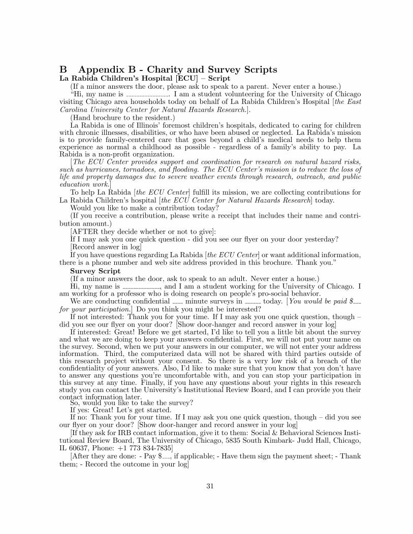
B Appendix B - Charity and Survey ScriptsLa Rabida Children’s Hospital [ECU] — Script(If a minor answers the door, please ask to speak to a parent. Never enter a house.)“Hi, my name is . I am a student volunteering for the University of Chicago

visiting Chicago area households today on behalf of La Rabida Children’s Hospital [the EastCarolina University Center for Natural Hazards Research.].(Hand brochure to the resident.)La Rabida is one of Illinois’ foremost children’s hospitals, dedicated to caring for children

with chronic illnesses, disabilities, or who have been abused or neglected. La Rabida’s missionis to provide family-centered care that goes beyond a child’s medical needs to help themexperience as normal a childhood as possible - regardless of a family’s ability to pay. LaRabida is a non-profit organization.[The ECU Center provides support and coordination for research on natural hazard risks,

such as hurricanes, tornadoes, and flooding. The ECU Center’s mission is to reduce the loss oflife and property damages due to severe weather events through research, outreach, and publiceducation work.]To help La Rabida [the ECU Center] fulfill its mission, we are collecting contributions for

La Rabida Children’s hospital [the ECU Center for Natural Hazards Research] today.Would you like to make a contribution today?(If you receive a contribution, please write a receipt that includes their name and contri-

bution amount.)[AFTER they decide whether or not to give]:If I may ask you one quick question - did you see our flyer on your door yesterday?[Record answer in log]If you have questions regarding La Rabida [the ECU Center] or want additional information,

there is a phone number and web site address provided in this brochure. Thank you.”Survey Script(If a minor answers the door, ask to speak to an adult. Never enter a house.)Hi, my name is , and I am a student working for the University of Chicago. I

am working for a professor who is doing research on people’s pro-social behavior.We are conducting confidential minute surveys in today. [You would be paid $

for your participation.] Do you think you might be interested?If not interested: Thank you for your time. If I may ask you one quick question, though —

did you see our flyer on your door? [Show door-hanger and record answer in your log]If interested: Great! Before we get started, I’d like to tell you a little bit about the survey

and what we are doing to keep your answers confidential. First, we will not put your name onthe survey. Second, when we put your answers in our computer, we will not enter your addressinformation. Third, the computerized data will not be shared with third parties outside ofthis research project without your consent. So there is a very low risk of a breach of theconfidentiality of your answers. Also, I’d like to make sure that you know that you don’t haveto answer any questions you’re uncomfortable with, and you can stop your participation inthis survey at any time. Finally, if you have any questions about your rights in this researchstudy you can contact the University’s Institutional Review Board, and I can provide you theircontact information later.So, would you like to take the survey?If yes: Great! Let’s get started.If no: Thank you for your time. If I may ask you one quick question, though — did you see

our flyer on your door? [Show door-hanger and record answer in your log][If they ask for IRB contact information, give it to them: Social & Behavioral Sciences Insti-

tutional Review Board, The University of Chicago, 5835 South Kimbark- Judd Hall, Chicago,IL 60637, Phone: +1 773 834-7835][After they are done: - Pay $ , if applicable; - Have them sign the payment sheet; - Thank

them; - Record the outcome in your log]

31

References

[1] Akerlof, George A. and Rachel E. Kranton. 2000. “Economics and Identity,” QuarterlyJournal of Economics, 115(3), 715-753.

[2] Andreoni, James. 1989. “Giving with Impure Altruism: Applications to Charity and Ri-cardian Equivalence.” Journal of Political Economy, 97(6), 1447-1458.

[3] Andreoni, James. 1990. Impure Altruism and Donations to Public Goods: A Theory ofWarm-Glow Giving. The Economic Journal, 100(401), 464-477.

[4] Andreoni, James. 2006. “Philantropy.”In Handbook of Giving, Altruism, and Reci-procity, ed. Serge-Christophe Kolm and Jean Mercier Ythier, 1201—1265. Amsterdam:Elsevier/North-Holland.

[5] Ariely, Dan, Anat Bracha, and Meier, Stephan. 2009. “Doing Good or Doing Well? Im-age Motivation and Monetary Incentives in Behaving Prosocially.” American EconomicReview, 99(1), 544-555.

[6] Asch, Solomon E. 1951. “Effects of Group Pressure Upon the Modification and Distortionof Judgment.” In H. Guetzkow (Ed.), Groups, leadership, and men. Pittsburgh: CarnegiePress.

[7] Bellemare, Charles, and Bruce Shearer. 2009. “On The Relevance and Composition ofGifts within the Firm: Evidence from Field Exeriments” Working paper.

[8] Benabou, Roland and Jean Tirole. 2006. “Incentives and Prosocial Behavior” AmericanEconomic Review, 96(5), 1652-1678.

[9] Bernheim, B. Douglas. 1994. “A Theory of Conformity” Journal of Political Economy,102(5), 841-877.

[10] Bodner, R. and Drazen Prelec. “The Diagnostic Value of Actions in a Self-Signaling Model,” in: I. Brocas and J.D. Carrillo, eds., The Psychology of Economic Decisions, Vol.1 ,Oxford University Press, 2002.

[11] Charness, Gary, and Rabin, Matthew. 2002. “Understanding Social Preferences with Sim-ple Tests.” Quarterly Journal of Economics 117(3), 817-869.

[12] Conlin, Michael, Ted O’Donoghue, and Timothy J. Vogelsang. 2007. “Projection Bias inCatalog Orders.” American Economic Review, 97(4), 1217-1249.

[13] Croson, Rachel and Shang, Jen. 2009. “A Field Experiment in Charitable Contribution:The Impact of Social Information on the Voluntary Provision of Public Goods.” EconomicJournal, 119, 1422-1439.

[14] Dana, Jason D., Daylian M. Cain, and Robyn M. Dawes. 2006. “What you don’t knowwon’t hurt me: Costly (but quiet) exit in dictator games.” Organizational Behavior andHuman Decision Processes, 100(2): 193-201.

[15] Dana, Jason, Roberto Weber, and Jason Xi Kuang. 2007. “Exploiting ‘Moral WriggleRoom’: Experiments Demonstrating an Illusory Preference for Fairness” Economic The-ory, 33, 67-80.

[16] DellaVigna, Stefano. 2009. “Psychology and Economics: Evidence from the Field” Journalof Economic Literature, 47(2), 315-372.

32

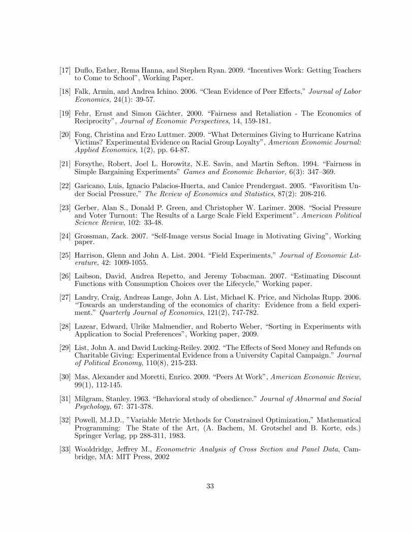
[17] Duflo, Esther, Rema Hanna, and Stephen Ryan. 2009. “Incentives Work: Getting Teachersto Come to School”, Working Paper.

[18] Falk, Armin, and Andrea Ichino. 2006. “Clean Evidence of Peer Effects,” Journal of LaborEconomics, 24(1): 39-57.

[19] Fehr, Ernst and Simon Gachter, 2000. “Fairness and Retaliation - The Economics ofReciprocity”, Journal of Economic Perspectives, 14, 159-181.

[20] Fong, Christina and Erzo Luttmer. 2009. “What Determines Giving to Hurricane KatrinaVictims? Experimental Evidence on Racial Group Loyalty”, American Economic Journal:Applied Economics, 1(2), pp. 64-87.

[21] Forsythe, Robert, Joel L. Horowitz, N.E. Savin, and Martin Sefton. 1994. “Fairness inSimple Bargaining Experiments” Games and Economic Behavior, 6(3): 347—369.

[22] Garicano, Luis, Ignacio Palacios-Huerta, and Canice Prendergast. 2005. “Favoritism Un-der Social Pressure,” The Review of Economics and Statistics, 87(2): 208-216.

[23] Gerber, Alan S., Donald P. Green, and Christopher W. Larimer. 2008. “Social Pressureand Voter Turnout: The Results of a Large Scale Field Experiment”. American PoliticalScience Review, 102: 33-48.

[24] Grossman, Zack. 2007. “Self-Image versus Social Image in Motivating Giving”, Workingpaper.

[25] Harrison, Glenn and John A. List. 2004. “Field Experiments,” Journal of Economic Lit-erature, 42: 1009-1055.

[26] Laibson, David, Andrea Repetto, and Jeremy Tobacman. 2007. “Estimating DiscountFunctions with Consumption Choices over the Lifecycle,” Working paper.

[27] Landry, Craig, Andreas Lange, John A. List, Michael K. Price, and Nicholas Rupp. 2006.“Towards an understanding of the economics of charity: Evidence from a field experi-ment.” Quarterly Journal of Economics, 121(2), 747-782.

[28] Lazear, Edward, Ulrike Malmendier, and Roberto Weber, “Sorting in Experiments withApplication to Social Preferences”, Working paper, 2009.

[29] List, John A. and David Lucking-Reiley. 2002. “The Effects of Seed Money and Refunds onCharitable Giving: Experimental Evidence from a University Capital Campaign.” Journalof Political Economy, 110(8), 215-233.

[30] Mas, Alexander and Moretti, Enrico. 2009. “Peers At Work”, American Economic Review,99(1), 112-145.

[31] Milgram, Stanley. 1963. “Behavioral study of obedience.” Journal of Abnormal and SocialPsychology, 67: 371-378.

[32] Powell, M.J.D., ”Variable Metric Methods for Constrained Optimization,” MathematicalProgramming: The State of the Art, (A. Bachem, M. Grotschel and B. Korte, eds.)Springer Verlag, pp 288-311, 1983.

[33] Wooldridge, Jeffrey M., Econometric Analysis of Cross Section and Panel Data, Cam-bridge, MA: MIT Press, 2002

33

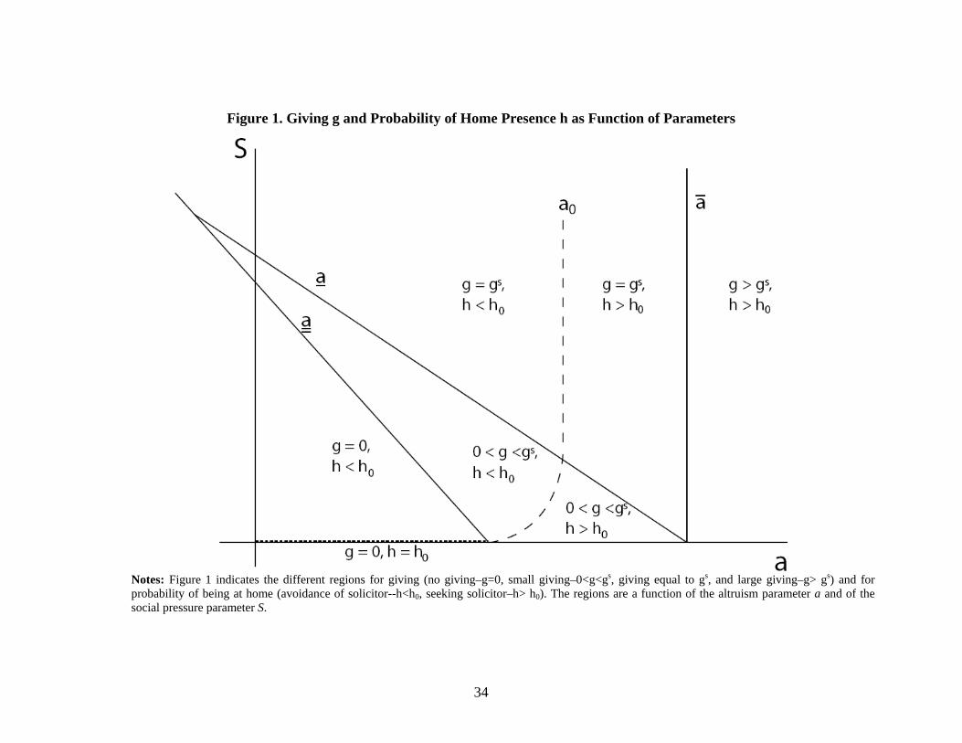
34

Figure 1. Giving g and Probability of Home Presence h as Function of Parameters

Notes: Figure 1 indicates the different regions for giving (no giving–g=0, small giving–0<g<gs, giving equal to gs, and large giving–g> gs) and for probability of being at home (avoidance of solicitor--h<h0, seeking solicitor–h> h0). The regions are a function of the altruism parameter a and of the social pressure parameter S.

35

Figure 2a. Summary of Door-to-Door Experimental Treatments Run in 2008

Figure 2b. Summary of Door-to-Door Experimental Treatments Run in 2009

Note: Figures 2a and 2b indicate the treatments run in the door-to-door field experiment respectively in 2008 (charity and survey) and in 2009 (survey only). La Rabida and ECU are the names of the two charities for which the fund-raising took place.

36

Figure 3. Examples of Flyers Utilized in the Field Experiment

Note: Figure 3 displays two examples of flyers for the fund-raising treatments (top row) and flyers for the 2008 survey treatments (bottom row). The top-left flyer is for the Opt-Out treatment, while the top-right flyer is for a Flyer treatment. The bottom-row flyers are both for a 10-minute survey with Flyer, the left one for no payment, the right one for a $10 payment.

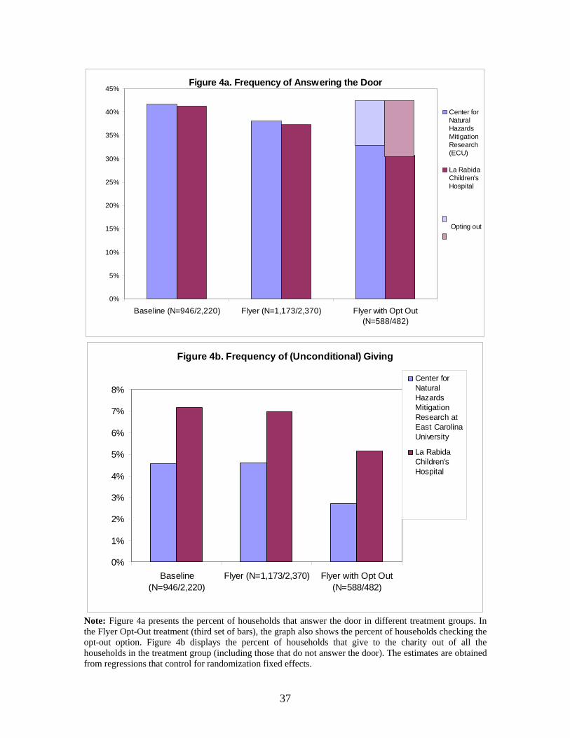
37

Figure 4a. Frequency of Answering the Door

0%

5%

10%

15%

20%

25%

30%

35%

40%

45%

Baseline (N=946/2,220) Flyer (N=1,173/2,370) Flyer with Opt Out(N=588/482)

Opting out

Center forNaturalHazardsMitigationResearch(ECU)

La RabidaChildren'sHospital

Figure 4b. Frequency of (Unconditional) Giving

0%

1%

2%

3%

4%

5%

6%

7%

8%

Baseline(N=946/2,220)

Flyer (N=1,173/2,370) Flyer with Opt Out(N=588/482)

Center forNaturalHazardsMitigationResearch atEast CarolinaUniversity

La RabidaChildren'sHospital

Note: Figure 4a presents the percent of households that answer the door in different treatment groups. In the Flyer Opt-Out treatment (third set of bars), the graph also shows the percent of households checking the opt-out option. Figure 4b displays the percent of households that give to the charity out of all the households in the treatment group (including those that do not answer the door). The estimates are obtained from regressions that control for randomization fixed effects.

38

Figure 4c. Frequency of Giving Conditional on Answering The Door

0%

2%

4%

6%

8%

10%

12%

14%

16%

18%

20%

Baseline (N=946/2,220) Flyer (N=1,173/2,370) Flyer with Opt Out(N=588/482)

Center forNatural HazardsMitigationResearch atEast CarolinaUniversity

La RabidaChildren'sHospital

Note: Figure 4c shows the results for giving conditioned on answering the door, which equals the ratio of the estimated unconditional giving (Figure 4b) and the estimated share of households answering the door (Figure 4a). The estimates are obtained from regressions that control for randomization fixed effects.

39

Figure 5a. Frequency of Giving: Small versus Large (pooled )

0.0%0.5%1.0%1.5%2.0%2.5%3.0%3.5%4.0%4.5%

Baseline(N=3,166)

Flyer (N=3,433) Flyer with Opt Out(N=1,070)

SmallDonations

LargeDonations

Note: Figure 5a presents the results on (unconditional) giving of small (<=$10) and large (> $10) donations across the treatments. The estimates are obtained from regressions that control for randomization fixed effects.

Figure 5b. Distribution of Amount Donated Under Different Treatments

0.00%

0.40%

0.80%

1.20%

1.60%

0-2 2 2-5 5 5-10 10 10-20 20 20-50 50 50+

Amount Donated ($)

Perc

enta

ge g

ivin

g sp

ecifi

ed a

mou

nt o

ut o

f all

hous

ehol

ds

Baseline (6.29% positivedonation)Flyer (5.85% positivedonation)Opt-Out (5.14% positivedonation)

Note: Figure 5b displays the distribution of money donated across different treatment groups. Each bar indicates the share of households giving the specified amount out of all households in the treatment. The Figure does not display the share of households donating $0. The estimates are obtained from regressions that control for randomization fixed effects.

40

Figure 6a. Survey (2008 Experiment)

0%

5%

10%

15%

20%

25%

30%

35%

40%

45%

Baseline ($0/10min)[N=607]

Flyer ($0/10min)[N=489]

Flyer ($0/5min)[N=450]

Flyer ($10/10min)[N=320]

Answeringthe Door

Completingthe Survey

Figure 6b. Survey (2009 Experiment)

0%

10%

20%

30%

40%

50%

60%

No Flyer($0/5min)

No Flyer($5/5min)

Flyer($0/10min)

Flyer($0/5min)

Flyer($5/5min)

Flyer($10/5min)

Opt-out($0/5min)

Opt-out($5/5min)

Answeringthe Door

Completingthe Survey

Opt-out

Note: Figures 6a and 6b present the effect of survey treatments run in 2008 (Figure 6a) and 2009 (Figure 6b) on the percent of household answering the door and on the percent completing the survey (out of all households). The estimates are obtained from regressions that control for randomization fixed effects.

41

Figure 7a. Distribution of Altruism and Cut-offs for Giving

Figure 7b. Overall Utility of Fund-Raiser as function of Altruism

. Note: Figures 7a plots the estimated distribution of the altruism parameter a. The Figure displays the threshold for giving $0 and for giving $10 in the absence of social pressure, given by au’(G+g)-1 > 0 or a > G+g. Figure 7b plots the implied utility in equilibrium of a standard door-to-door fund-raiser, as a function of the altruism parameter a. The parameter values are from the benchmark minimum distance estimates (Column (1) in Table 4).

42

Panel A: Fund-Raising Treatments

Variable:Sample: Pooled ECU La Rabida Pooled ECU La Rabida ECU La Rabida

(1) (2) (3) (4) (5) (6) (7) (8)0.409 0.4228 0.4032 0.0629 0.0507 0.0680

0.3753 0.3993 0.3628 0.0585 0.0460 0.06500.3355 0.3503 0.3174 0.0514 0.0289 0.0788

N = 7668 N = 2706 N = 4962 N = 7668 N = 2706 N = 4962 N = 2706 N = 4962

Panel B: Survey Treatments

Variable:

Share of Hhs. Answering the

Door

Share of Hhs. Completing the

Survey2008 Survey Treatments 2009 Survey Treatments (3) (4)

0.4279 0.14710.4417 0.12630.4155 0.13900.4288 0.16980.4515 0.20710.4772 0.25630.3645 0.14040.3963 0.1807

N N = 9903 N = 9903

Flyer ($5/5min)Flyer ($10/10min)Opt-Out ($0/5min)Opt-Out ($0/10min)

Baseline ($0/5min)Baseline ($5/5min)Flyer ($0/10min)Flyer ($0/5min)

0.09720.11860.17140.1719

Zero donations across all treatments

One ($25) donation across all

treatments

Share of Households Answering the Door

(1)

Share of Households Completing the

Survey(2)

Notes: Summary statistics for the variables of the experiment. "ECU" and "La Rabida" indicate the two charities in the experiment, "ECU" is an out-of-state research center on hurricanes, "La Rabida" is an in-statechildren's hospital.

N N = 1865N = 1865Flyer ($10/10min) Treatment 0.4156Flyer ($0/5min) Treatment 0.392Flyer ($0/10min) Treatment 0.3681Baseline ($0/10min) Treatment 0.4135

Flyer with Opt-out TreatmentN

Table 1. Summary Statistics -- Treatment Outcomes

Share of Households Answering the Door

Baseline (No-Flyer) Treatment

Share of Households Giving (In-Person)

Number of Households Giving (Mail/Internet)

Flyer Treatment

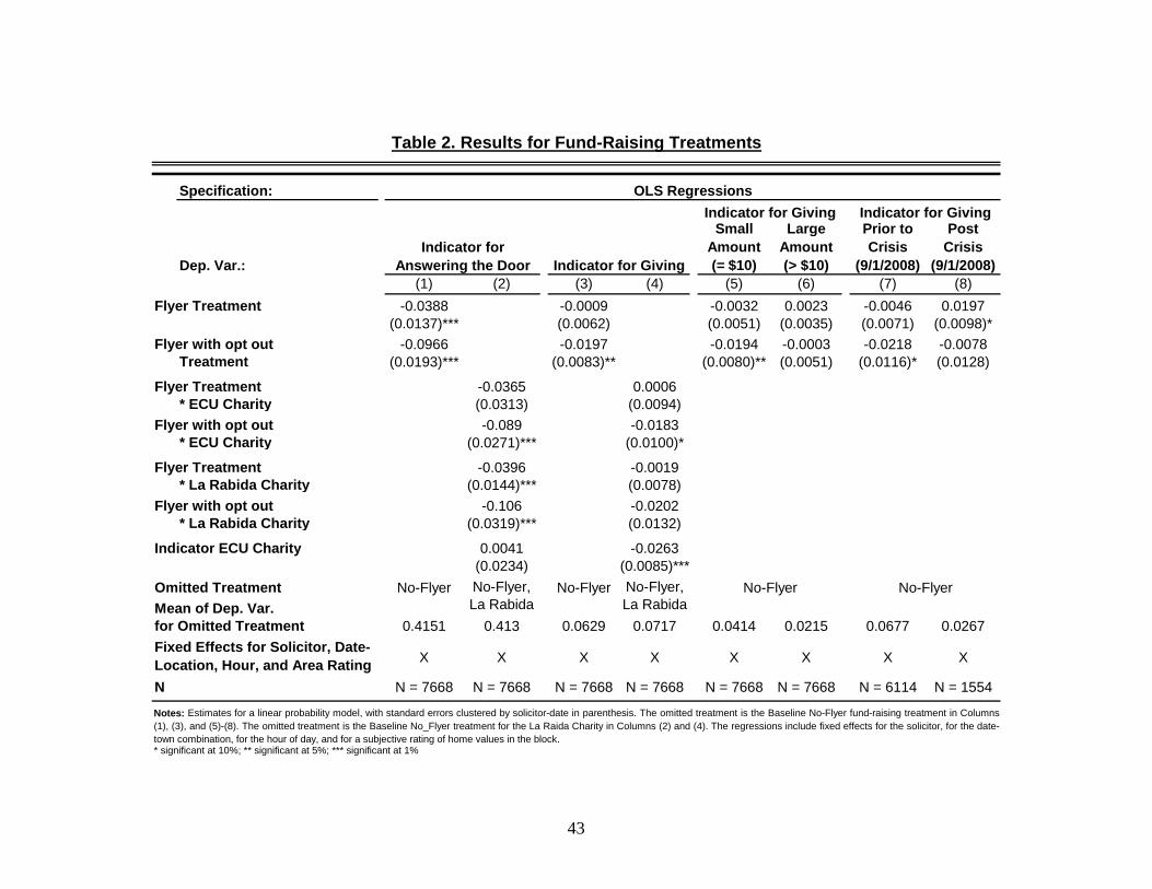
43

Specification:

Dep. Var.:

Small Amount (= $10)

Large Amount (> $10)

Prior to Crisis

(9/1/2008)

Post Crisis

(9/1/2008)(1) (2) (3) (4) (5) (6) (7) (8)

-0.0388 -0.0009 -0.0032 0.0023 -0.0046 0.0197(0.0137)*** (0.0062) (0.0051) (0.0035) (0.0071) (0.0098)*

-0.0966 -0.0197 -0.0194 -0.0003 -0.0218 -0.0078Treatment (0.0193)*** (0.0083)** (0.0080)** (0.0051) (0.0116)* (0.0128)

-0.0365 0.0006* ECU Charity (0.0313) (0.0094)

-0.089 -0.0183* ECU Charity (0.0271)*** (0.0100)*

-0.0396 -0.0019* La Rabida Charity (0.0144)*** (0.0078)

-0.106 -0.0202* La Rabida Charity (0.0319)*** (0.0132)

0.0041 -0.0263(0.0234) (0.0085)***

No-Flyer No-FlyerMean of Dep. Var.

0.4151 0.413 0.0629 0.0717 0.0414 0.0215 0.0677 0.0267

X X X X X X X X

N = 7668 N = 7668 N = 7668 N = 7668 N = 7668 N = 7668 N = 6114 N = 1554

No-Flyer No-FlyerNo-Flyer, La Rabida

No-Flyer, La Rabida

N

Notes: Estimates for a linear probability model, with standard errors clustered by solicitor-date in parenthesis. The omitted treatment is the Baseline No-Flyer fund-raising treatment in Columns(1), (3), and (5)-(8). The omitted treatment is the Baseline No_Flyer treatment for the La Raida Charity in Columns (2) and (4). The regressions include fixed effects for the solicitor, for the date-town combination, for the hour of day, and for a subjective rating of home values in the block.* significant at 10%; ** significant at 5%; *** significant at 1%

Flyer with opt out

for Omitted TreatmentFixed Effects for Solicitor, Date-Location, Hour, and Area Rating

Flyer Treatment

Flyer with opt out

Flyer Treatment

Omitted Treatment

Table 2. Results for Fund-Raising Treatments

OLS RegressionsIndicator for Giving Indicator for Giving

Flyer with opt out

Indicator ECU Charity

Indicator for Answering the Door Indicator for Giving

Flyer Treatment

44

Specification:Sample:

Dependent Variable:

Indicator for Answering the

Door

Indicator for Completing

Survey

Indicator for Answering the

Door

Indicator for Completing

Survey(1) (2) (3) (4)

-0.0563 0.0000(0.0377) (0.0260)-0.0021 0.0794(0.0334) (0.0233)***-0.0105 0.0695(0.0448) (0.0265)**

-0.0059 -0.0217(0.0206) (0.0175)-0.0187 -0.0043(0.0260) (0.0192)-0.0158 0.0224(0.0199) (0.0133)*0.0185 0.0526

(0.0214) (0.0168)***0.0405 0.1042

(0.0243)* (0.0179)***-0.0727 -0.0056

(0.0209)*** (0.0161)-0.0413 0.0247

(0.0193)** (0.0161)

0.4138 0.1025 0.4373 0.1498Omitted Treatment

X X X X

N = 1865 N = 1865 N = 9896 N = 9896

Table 3. Results for Survey Treatments

Mean of Dep. Var. for

Flyer ($0/5min) Treatment

Flyer ($10/10min) Treatment

Baseline ($5/5min) Treatment

Flyer ($0/10min) Treatment

Flyer ($5/5min) Treatment

Flyer ($10/5min) Treatment

Opt-Out ($0/5min) Treatment

* significant at 10%; ** significant at 5%; *** significant at 1%

Fixed Effects for Solicitor, Date-Location, Hour, and Area RatingN

Notes: Estimates for a linear probability model, with standard errors clustered by solicitor-date in parenthesis. The first two columns refer to door-to-door survey tretaments run in 2008, while the next two columns refer to door-to-door survey treatments run in 2009. The omitted treatment is theBaseline No-Flyer $0-10 minutes survey for Columns (1) and (2) and the Baseline No-Flyer $0-5 minutes survey for Columns (3) and (4). Theregressions include fixed effects for the solicitor, for the date-town combination, for the hour of day, and for a subjective rating of home values in theblock.

OLS Regressions2008 Survey 2009 Survey

Flyer ($0/5min) Treatment

Flyer ($0/10min) Treatment

Omitted Treatment Baseline ($0/10min) Baseline ($0/5min)

Opt-Out ($5/5min) Treatment

45

Common Parameters

Survey Parameters

Charity Parameters La Rabida ECU La Rabida ECU-13.894 -10.615 -16.519 -19.399(3.273) (4.238) (3.895) (5.366)22.061 16.676 19.287 18.798(1.304) (1.850) (3.885) (4.088)

Curvature of Altruism Function (G)

3.528 1.363 4.022 2.459(0.611) (0.742) (1.571) (1.642)

(1) (2)

Value of Time of One-Hour Survey

Prob. Answering Door (h) - Year 2008

Prob. Answering Door (h) - Year 2009

Prob. Observing Flyer (r)

Elasticity of Home Presence (eta)

76.761

(0.007) (0.008)0.446 0.448

-25.913(4.500)28.144(4.994)

(26.130)4.478

(1.658)

0.413(0.006)

0.313(0.010)0.045

(0.018)0.111

Notes: Estimates from minimum-distance estimator with moments listed in Appendix Table 1 and weights given by inverse of diagonal of variance-covariance matrix in Column (1) and given by identity matrix in Column (2). Standard errors are in parentheses.

-26.233(4.074)29.840(5.051)74.580

(22.901)

Table 4. Minimum-Distance Estimates: Benchmark Results

Social Pressure Cost of Giving 0 in Person

Mean Utility (in $) of Doing 10-Minute Survey

Std. Dev. of Utility of Doing Survey

0.414(0.005)

0.301(0.010)0.050

(0.015)

Estimates with Identity Weighting Matrix

Implied Cost of Altering Prob. Home by 10 pp.

Mean Weight on Altruism Function (mu)

Std. Dev. of Weight on Altruism Function

Benchmark Estimates

0.099

Social Pressure Cost of Saying No to Survey 4.219(1.193)

12.272 5.801(5.116) (9.008)

46

Common ParametersProb. Observing Flyer (r)

Elasticity of Home Presence(eta)

Probability of Type withSocial Preferences (p)

Survey Parameters

10-Minute Survey

10-Minute Survey

of Saying No to Survey

Charity ParametersLa

Rabida ECULa

Rabida ECULa

Rabida ECULa

Rabida ECULa

Rabida ECULa

Rabida ECU-13.894 -10.615 -12.531 -8.025 -15.658 -14.358 -13.074 -9.375 - - -1.402 0.257

Function (3.273) (4.238) (5.680) (6.513) (6.238) (7.676) (4.138) (5.043) - - (6.820) (7.359)22.061 16.676 22.077 15.953 21.784 17.414 22.627 16.887 - - 19.396 14.818

Altruism Function (1.304) (1.850) (1.278) (1.601) (1.283) (2.374) (1.417) (1.917) - - (1.437) (1.559)Curvature of Altruism - -

Function (G) - -3.528 1.363 2.556 0.630 4.081 2.073 3.333 1.290 - - 3.231 1.030

of Giving 0 in Person (0.611) (0.742) (0.754) (0.612) (2.421) (2.028) (0.667) (0.711) - - (0.676) (0.668)Decomposition of Giving and WelfareShare of Givers who Seek 0.510 0.517 0.545 0.613 0.519 0.496 0.504 0.508 - - 0.490 0.532

The Fund-raiser (0.040) (0.095) (0.041) (0.148) (0.043) (0.103) (0.040) (0.096) - - (0.038) (0.099)-1.042 -0.425 -0.689 -0.146 -1.211 -0.687 -0.993 -0.410 - - -0.471 -0.144

of Fund-Raiser (in $) (0.155) (0.286) (0.190) (0.235) (0.916) (0.811) (0.169) (0.274) - - (0.145) (0.152)

-15.850(3.216)22.746(4.100)

(0.0709)

15.791

More Detailed Giving Moments

0.303(0.010)0.066

(0.025)

-25.599

Only Survey Moments

0.550(0.089)

0.6219

0.026(0.007)

0.317(0.014)0.048

(0.026)

----

Allows for no social pref.

0.270

13.991(6.247)

-

0.062(0.023)

30.468

(4)

Average Welfare per Househ

0.050 0.046(0.015) (0.024)

(3.984)29.594(4.963)

(5.116) (6.780) (7.295)(7.333)12.272 10.04413.333

Social Pressure Cost 4.219(1.193)

Mean Weight on Altruism

Std. Dev. of Weight on

Benchmark Estimates

Less Detailed Giving Moments

3.351(1.213)

(1) (2)

Table 5. Minimum Distance Estimates: Robustness

Social Pressure Cost

Mean Utility (in $) of Doing

Std. Dev. of Utility of Doing

0.301(0.010)

Notes: Estimates from minimum-distance estimator with moments listed in Appendix Table 1 and weights given by inverse of diagonal of variance-covariance matrix. Benchmark estimates in Column (1) use giving moments(0,10), 10, (10,20], (20,50], 50+. Estimates in Column (2) use giving moments (0,3], (3,7], (7,10], (10,20], (20,50], 50+. Estimates in Column (3) use giving moments (0,10], (10,20], (20,50], 50+. Estimates in Column (4) do notuse any of the survey moments, while estimates in Column (5) only use the survey moments. Estimates in Columns allow for a share (1-p) of the population that have no altruism, nor social pressure. These agents do not giveto charity and do not complete the survey. Standard errors are in parentheses.

-26.233(4.074)29.840(5.051)

-26.544(4.384)29.984

-26.556(4.506)

0.300(0.011)

(5.283)

(3) (5)

(0.017)

4.559 4.107(2.130)

9.651(2.351)(2.117)

No Survey Moments

(6)

-

(5.150)

47

Specification:Charity: La Rabida Charity ECU Charity

(1) (2)Panel A. Decomposition of Giving in Standard (No-Flyer) Fund-raiserShare of Givers Who Would Give 0.731 0.836

Without Social Pressure (S=0 ) (0.054) (0.084)Share of Amount That Would Be Given 0.726 0.810

Without Social Pressure (S=0 ) (0.029) (0.096)Share of Givers who Seek 0.510 0.517

the Fund-raiser ('Happy Givers') (0.040) (0.095)

Panel B. Sorting in Fund-raiser with FlyerIncrease in Answering the Door due to 0.007 0.003

Altruism ('Sorting In') (0.001) (0.001)Decrease in Answering the Door due to -0.048 -0.019

Social Pressure ('Sorting Out') (0.011) (0.011)

Panel C. Welfare

Welfare per Household Contacted (in $) -1.042 (0.155) -0.425 (0.286)Money Raised per Household Contacted 0.726 (0.036) 0.332 (0.046)Money Raised per Household, Net of Salary 0.346 (0.036) -0.048 (0.046)

Welfare per Household Contacted (in $) -0.569 (0.114) -0.327 (0.243)Money Raised per Household Contacted 1.165 (0.081) 0.508 (0.088)Money Raised per Household, Net of Salary 0.785 (0.036) 0.128 (0.046)

Welfare per Household Contacted (in $) 0.456 (0.147) 0.156 (0.064)Money Raised per Household Contacted 1.015 (0.092) 0.451 (0.092)Money Raised per Household, Net of Salary 0.635 (0.036) 0.071 (0.046)

Welfare in Fund-Raiser with Opt-out (r=1)

Welfare in Standard (No-Flyer) Fund-Raiser

Table 6. Decomposition of Giving and Welfare

Welfare in Fund-Raiser with Flier (r=1)

Minimum-Distance Benchmark Estimates

Notes: Decomposition, sorting, and welfare are computed using estimates from minimum-distance estimator with weights given byinverse of diagonal of variance-covariance matrix (Column (1) in Table 4). In the welfare computations for the Flyer and Opt-outtreatments, we assume that 100 percent of households see the flyer, that is, r=1. To compute the salary cost of the solicitor we assume25 households reached in one hour and an hourly wage of $9.5. Standard errors are in parentheses.

48

Specification:Charity

Empirical Moments

Estimated Moments

Empirical Moments

Estimated Moments

Panel A: Fund-Raising Moments (1) (2) (3) (4)0.4130 0.4136 0.4171 0.41360.3733 0.3730 0.3806 0.39760.3070 0.3064 0.3281 0.29890.1202 0.1142 0.0988 0.11790.0717 0.0666 0.0455 0.04200.0699 0.0709 0.0461 0.04460.0515 0.0639 0.0272 0.03920.0245 0.0254 0.0303 0.02690.0163 0.0178 0.0118 0.02090.0233 0.0228 0.0268 0.02630.0216 0.0203 0.0051 0.00510.0138 0.0189 0.0014 0.00560.0200 0.0209 0.0041 0.00560.0137 0.0134 0.0084 0.00790.0083 0.0165 0.0136 0.00970.0186 0.0165 0.0125 0.00970.0103 0.0074 0.0020 0.00210.0138 0.0106 0.0008 0.00300.0078 0.0106 0.0030 0.00300.0016 0.0001 -0.0003 0.0000-0.0006 0.0002 -0.0005 0.00000.0002 0.0002 -0.0002 0.0000

N = 4962 N = 4962 N = 2707 N = 2707

Empirical Moments

Estimated Moments

Empirical Moments

Estimated Moments

Empirical Moments

Estimated Moments

Panel B: Survey Moments (1) (2) (3) (4) (5) (6)Moments 2008

0.4138 0.4136 0.1025 0.0953 - -0.3576 0.3883 0.1025 0.1192 - -0.4118 0.4016 0.1819 0.1562 - -0.4033 0.4108 0.1720 0.1813 - -

N = 1866 N = 1866 N = 1866 N = 1866 - -Moments 2009

0.4373 0.4461 0.1498 0.1331 - -0.4312 0.4461 0.1281 0.1600 - -0.4182 0.4198 0.1455 0.1256 - -0.4210 0.4311 0.1722 0.1639 - -0.4558 0.4439 0.2024 0.2003 - -0.4784 0.4579 0.2538 0.2374 - -

Opt-out $0, 5min 0.3648 0.3714 0.1442 0.1579 0.1324 0.1099Opt-out $5, 5min 0.3958 0.3883 0.1744 0.1937 0.0867 0.1017

N = 9896 N = 9896 N = 9896 N = 9896 N = 9896 N = 9896

Appendix Table 1. Empirical Moments and Estimated Moments

No Flyer $5, 5minFlyer $0, 10minFlyer $0, 5min

Flyer $10, 5min

P(Do Survey) P(Opt-out)

N

No Flyer $0, 5min

P(Giving>50), No Flyer

P(Giving>50), Opt-outN

P(Home)

P(0<Giving<10), FlyerP(0<Giving<10), Opt-out

P(10<Giving<=20), Flyer

Flyer $0, 10min

P(Giving=10), No FlyerP(Giving=10), FlyerP(Giving=10), Opt-out

Flyer $0, 5min

Flyer $5, 5min

NNotes: The Table presents the empirical moments and the estimated moments from a minimum-distance estimator. The empirical moments are obtained as regression estimates after controlling for the randomization fixed effects and as such can occasionally be negative. The minimum-distance estimates are in Table 4, Column (1).

P(Giving) Flyer

P(Opt Out) Opt-Out

P(Giving>50), Flyer

No Flyer $0, 10min

Flyer $10, 10min

Minimum-Distance Estimates

P(Home) No FlyerP(Home) Flyer

La Rabida Charity ECU Charity

P(Home) Opt-Out

P(Giving) No Flyer

P(Giving) Opt-OutP(0<Giving<10), No Flyer

P(10<Giving<=20), No Flyer

P(10<Giving<=20), Opt-outP(20<Giving<=50), No FlyerP(20<Giving<=50), FlyerP(20<Giving<=50), Opt-out