Revealed Altruism -
46
Revealed Altruism By James C. Cox, Daniel Friedman, and Vjollca Sadiraj Forthcoming in Econometrica
Transcript of Revealed Altruism -
Revealed Altruism
By James C. Cox, Daniel Friedman, and Vjollca Sadiraj
Forthcoming in Econometrica
REVEALED ALTRUISM
BY JAMES C. COX, DANIEL FRIEDMAN, AND VJOLLCA SADIRAJ
Abstract. This paper develops a nonparametric theory of preferences
over one�s own and others�monetary payo¤s. We introduce �more altruis-
tic than� (MAT), a partial ordering over such preferences, and interpret
it with known parametric models. We also introduce and illustrate �more
generous than�(MGT), a partial ordering over opportunity sets. Several
recent studies focus on two player extensive form games of complete in-
formation in which the �rst mover (FM) chooses a more or less generous
opportunity set for the second mover (SM). Here reciprocity can be for-
malized as the assertion that an MGT choice by the FM will elicit MAT
preferences in the SM. A further assertion is that the e¤ect on preferences is
stronger for acts of commission by FM than for acts of omission. We state
and prove propositions on the observable consequences of these assertions.
Finally, empirical support for the propositions is found in existing data
from Investment and Dictator games, the Carrot and Stick game, and the
Stackelberg duopoly game and in new data from Stackelberg mini-games.
Keywords: Neoclassical Preferences, Social Preferences, Convexity, Reci-
procity, Experiments.
1. Introduction
What are the contents of preferences? People surely care about their own
material well-being, e.g., as proxied by income. In some contexts people also
may care about others�well-being. Abstract theory and common sense have
long recognized that possibility but until recently it has been neglected in
applied work. Evidence from the laboratory and �eld (as surveyed in Fehr and
Gächter (2000), for example) has begun to persuade economists to develop
speci�c models of how and when a person�s preferences depend on others�
material payo¤s (Sobel (2005)).
0For helpful comments, we thank James Andreoni, Geert Dhaene, Steven Gjerstad, StephenLeider, Joel Sobel, Stefan Traub, and Frans van Winden as well as participants in theInternational Meeting of the Economic Science Association (ESA) 2004, the North AmericanRegional ESA Meeting 2004, and at Economics Department seminars at UCSC, Harvardand University College London. The �nal revision is much improved due to the suggestionsof three anonymous referees and Associate Editor David Levine. Financial support wasprovided by the National Science Foundation (grant numbers IIS-0630805 and IIS-0527770).
1
2 BY JAMES C. COX, DANIEL FRIEDMAN, AND VJOLLCA SADIRAJ
Andreoni and Miller (2002) report �dictator� experiments in which a hu-
man subject decides on an allocation for himself and for some anonymous
other subject while facing a linear budget constraint. Their analysis con�rms
consistency with the generalized axiom of revealed preference (GARP) for a
large majority of subjects. They conclude that altruism can be modeled using
neoclassical preference theory (Hicks (1939), Samuelson (1947)).
In this paper we take three further steps down the same path. First, we
analyze non-linear opportunity sets. Such sets allow a player to reveal more
about the tradeo¤ between her own and another�s income, e.g., whether her
indi¤erence curves have positive or negative slope, and whether they are linear
or strictly convex. Second, we give another player an initial move that can
be more or less generous. This allows us to distinguish conditional altruism�
positive and negative reciprocity� from unconditional altruism. It also allows
us to clarify the observable consequences of convex preferences and of recip-
rocal preferences. Third, we distinguish active from passive initial moves; i.e.,
we distinguish among acts of omission, acts of commission, and absence of
opportunity to act, and examine their impacts on reciprocity.
Our goal is to develop an approach to reciprocity �rmly grounded in neo-
classical preference and demand theory.1 By contrast, much of the existing
literature on social preferences either ignores reciprocity motives or grounds
them in psychological game theory. Our focus is on how players�choices re-
spond to observable events and opportunities, rather than to their beliefs about
other players�intentions or types.
Section 2 begins by developing representations of preferences over own and
others�income, and formalizes the idea that one preference ordering is �more
altruistic than�(MAT) another. It allows for the possibility of negative re-
gard for the other�s income; in this case MAT really means �less malevolent
than.� Special cases include the main parametric models of other-regarding
preferences that have appeared in the literature.
Section 3 introduces opportunities and formalizes the idea that one oppor-
tunity set can be more generous than (MGT) another. It explains thatMGT
is a partial ordering over standard budget sets and is a complete ordering over
opportunity sets in several two player games, including the well-known Invest-
ment, Dictator, and Stackelberg duopoly games. An appendix demonstrates
1Cox, Friedman and Gjerstad (2007) takes a similar perspective, but it imposes a tightparametric structure (CES) on preferences and reports structural estimates from variousexisting data sets. Here we seek general results attributable to general properties such asconvexity and reciprocity, and we test the results directly on new as well as existing data.
REVEALED ALTRUISM 3
MGT orderings of opportunity sets for several other games in the literature
on social preferences.
Section 4 formalizes reciprocity. Axiom R asserts that more generous choices
by a �rst mover induce more altruistic preferences in a second mover. An in-
terpretation (advocated in Cox, Friedman, and Gjerstad (2007)) is that prefer-
ences are emotional state-dependent, and the �rst mover�s generosity induces
a more benevolent (or less malevolent) emotional state in the second mover.
Axiom S asserts that the reciprocity e¤ect is stronger following an act of com-
mission (upsetting the status-quo) than following an act of omission (upholding
the status-quo), and that the e¤ect is weaker when the �rst mover is unable
to alter the status quo.
Section 5 presents three general theoretical propositions on the consequences
of convex preferences. Among other things, these propositions extend standard
results on revealed preference theory and show how easy it is in empirical work
to con�ate the separate e¤ects of convexity and reciprocity.
Sections 6 - 9 bring revealed altruism theory to four data sets. Proposition
4 derives testable predictions for Investment and Dictator games. Together,
these two games provide diagnostic data for both Axiom R and Axiom S.
Propositions 5 and 6 derive testable predictions for Carrot and Stick games
and for Stackelberg duopoly games. The duopoly games are especially useful
because the Follower�s opportunity sets are MGT-ordered and have a para-
bolic shape that enables the Follower to reveal a wide range of positive and
negative tradeo¤s between his own income and Leader�s income. Proposition 7
obtains predictions for a new variant game, called the Stackelberg mini-game,
in which the Leader has only two alternative output choices, one of which is
clearly more generous than the other. This game provides diagnostic data for
discriminating between the e¤ects of convexity and reciprocity.
Within the limitations of the data, the test results are consistent with pre-
dictions. Following a concluding discussion, Appendix A collects all formal
proofs and other mathematical details. Instructions to subjects in the Stack-
elberg mini-game appear in Appendix B.
2. Preferences
Let Y = (Y1; Y2; :::; YN) 2 RN+ represent the payo¤ vector in a game that
pays each of N � 2 players a non-negative income. Admissible preferences
for each player i are smooth and convex orderings on the positive orthant
<N+ that are strictly increasing in own income Yi. The set of all admissible
4 BY JAMES C. COX, DANIEL FRIEDMAN, AND VJOLLCA SADIRAJ
preferences is denoted P. Any particular preference P 2 P can be representedby a smooth utility function u : <N+ ! < with positive ith partial derivative@u=@Yi = uYi > 0: The other �rst partial derivatives are zero for standard
sel�sh preferences, but we allow for the possibility that they are positive in
some regions (where the agent is �benevolent�) and negative in others (where
she is �malevolent�).
We shall focus on two-player extensive form games of complete information,
and to streamline notation we shall denote own (�my�) income by Yi = m and
the other player�s (�your�) income by Y�i = y. Thus preferences are de�ned
on the positive quadrant <2+ = f(m; y) : m; y � 0g: The marginal rate ofsubstitution MRS(m; y) = um=uy is not well de�ned at points where the agent
is sel�sh; it diverges to +1 and back from �1 when we pass from slight
benevolence to slight malevolence. Therefore it is convenient to work with
willingness to pay, WTP= 1=MRS, the amount of own income the agent is
willing to give up in order to increase the other agent�s income by a unit; it
moves from slightly positive through zero to slightly negative when the agent
goes from slight benevolence to slight malevolence. Note that WTP= uy=umis intrinsic, independent of the particular utility function u chosen to represent
the given preferences.
What sort of factors might a¤ect w =WTP? Of course, for admissible pref-
erences the sign of w is the same as the sign of the partial derivative uy:
Convexity tells us more: w increases as one moves southward along an indif-
ference curve. That is, my benevolence increases (or malevolence decreases)
as your income decreases along an indi¤erence curve. This principle is quite
intuitive, and sometimes it is useful to strengthen it as follows. We say that ad-
missible preferences have the increasing benevolence (IB) property if wm � 0.Occasionally we refer to the related property wy � 0. Appendix A.1 shows
how convexity, increasing benevolence, and homotheticity are related to each
other and to the slope and curvature of indi¤erence curves.
We are now prepared to formalize the idea that one preference ordering
on <2+ is more altruistic than another. Two di¤erent preference orderingsA;B 2 P over income allocation vectors might represent the preferences of
two di¤erent players, or might represent the preferences of the same player in
two di¤erent situations.
De�nition 1. For a given domain D� <2+ we say that A MAT B on D if
WTPA(m; y) �WTPB(m; y); for all (m; y) 2D.
REVEALED ALTRUISM 5
The idea is straightforward. Like the single crossing property in a di¤erent
context,MAT induces a partial ordering on preferences over own and others�
income. In the benevolence case, A MAT B means that A has shallower
indi¤erence curves than B in (m; y) space, so A indicates a willingness to paymore m for a unit increase in y than does B. In the malevolence case, WTP isless negative for A, so it indicates a lesser willingness to pay for a unit decreasein y.
Appendix A.2 veri�es that MAT is a partial ordering on P. When no
particular domain D is indicated, theMAT ordering is understood to refer to
the entire positive orthant D= <2+.Four examples illustrate howMAT is incorporated into existing parametric
models.
Example 2.1. Linear Inequality-averse Preferences (for N = 2 only; Fehr
and Schmidt (1999)). Let preferences J = A;B be represented by uJ (m; y) =(1 + �J )m� �J y; where
�J = �J ; if m < y
= ��J ; if m � y;
with �J � �J and 0 < �J < 1. Straightforwardly, A MAT B if and only if�A � �B.
Example 2.2. Nonlinear Inequality-averse Preferences (forN = 2; Bolton and
Ockenfels (2000)). Let preferences J = A;B be represented by uJ (m; y) =�J (m;�); where
� = m=(m+ y); if m+ y > 0
= 1=2; if m+ y = 0:
It can be easily veri�ed that A MAT B if and only if �A1=�A2 � �B1=�B2.
Example 2.3. Quasi-maximin Preferences (for N = 2; Charness and Rabin
(2002)). Let preferences J = A;B be represented by
uJ (m; y) = m+ J (1� �J )y; if m < y
= (1� �J J )m+ J y; if m � y;
and J 2 [0; 1], �J 2 (0; 1). It is straightforward (although a bit tedious) toverify that A MAT B if and only if
A � Bmax�
1
1 + (�A � �B) B;1� �B1� �A
�:
6 BY JAMES C. COX, DANIEL FRIEDMAN, AND VJOLLCA SADIRAJ
Example 2.4. Egocentric Altruism (CES) Preferences (Cox and Sadiraj
(2007)). Let preferences J=A;B be represented by
uJ (m; y) =1
�(m� + �J y
�); if � 2 (�1; 1)�f0g
= my�J ; if � = 0:
If 0 < �B � �A then A MAT B. Veri�cation is straightforward: WTPJ =�J (m=y)
1��, J = A;B imply WPTA=WTPB = �A=�B � 1: �Egocentricity�
means that uJ (x+ �; x� �) > uJ (x� �; x+ �) for any � 2 (0; x) which impliesWTP (m;m) � 1:
Much of the theoretical literature on social preferences relies on special as-
sumptions that may appear to be departures from neoclassical preference the-
ory (Hicks (1939), Samuelson (1947)). The preceding examples help clarify
the issues. All four are examples of convex preferences, and (except for the
nonlinear inequality aversion model) they are also homothetic. The inequality
aversion models incorporate a very speci�c inconsistency with the neoclassical
assumption of positive monotonicity: my marginal utility for your income re-
verses sign on the 45 degree line. A preference for e¢ ciency (i.e., for a larger
income sum) is consistent with a limiting case of the quasi-maximin model,
or with admissible preferences with WTP = 1. We shall now see that for
more general preferences, the e¢ ciency of choices depends on the shape of the
opportunity set.
3. Opportunities
De�ne an opportunity set F (or synonymously, a feasible set or budget set) as a
convex compact subset of <2+: It is convenient and harmless (given preferencesmonotone in own income m) to assume free disposal for own income, i.e., if
(m; y) 2 F then (am; y) 2 F for all a 2 [0; 1]. Thus an opportunity set F is
the convex hull of two lines: (a) its projection YF = fy � 0 : 9m � 0 s:t:
(m; y) 2 Fg on the y-axis, and (b) its Eastern boundary @EF = f(m; y) 2 F :8x > m; (x; y) =2 Fg.Since F is convex, each boundary point has a supporting hyperplane (i.e.,
tangent line) de�ned by an inward-pointing normal vector, and F is contained
in its closed positive halfspace; see for example Rockafellar (1970, p. 100).
At some boundary points (informally called corners or kinks) the supporting
hyperplane is not unique; examples will be noted later. At the other (regular)
boundary points there is a smooth function f whose zero isoquant de�nes the
boundary locally. We often need to work near vertical tangents, so rather
REVEALED ALTRUISM 7
than the usual marginal rate of transformation (MRT) we use the need to pay,
NTP(m; y) = 1=MRT(m; y) = fy=fm evaluated at a regular point (m; y) 2@EF . Again NTP is intrinsic, independent of the choice f used to represent
the boundary segment.
We seek an objective de�nition of one opportunity setG being more generous
to me than another opportunity set F . There is an obvious necessary condition:
that G allows me to achieve higher income than does F . Since my preferences
are monotone in own income, I clearly bene�t when you allow me to increase
it. For some purposes it is helpful to impose a second condition, that you don�t
increase your own potential income far more than mine. If you do, I might
regard your move as self-serving and not especially generous.
These intuitions are captured in conditions (a) and (b) below, using the
following notation. Let y�F = supYF denote your maximum feasible income
and let m�F = supfm : 9y � 0 s:t: (m; y) 2 Fg denote my maximum feasible
income in an opportunity set F .
De�nition 2. Opportunity set G � <2+ is more generous than opportunityset F � <2+ if (a) m�
G �m�F � 0 and (b) m�
G �m�F � y�G � y�F : In this case we
write G MGT F .
MGT is a partial ordering over opportunity sets, as noted in Appendix
A.3. Condition (a) seems compelling because it springs directly from the most
basic intuitions about generosity, but one can imagine plausible variants on
condition (b). To understand its role, consider an alternative de�nition of
MGT, call it MGT Light, that includes only condition (a). It turns out
that MGT Light has the same implications as MGT for ten of the twelve
prominent examples of opportunity sets from the social preferences literature
discussed in this section, section 9 and Appendix A.5. We begin with a very
prominent example where condition (b) does matter.
Example 3.1. Standard budget set. Let F =�(m; y) 2 <2+ : m+ py � I
for given p; I > 0. Then the Eastern boundary @EF is the budget line�(m; y) 2 <2+ : m+ py = I
, as shown by the solid line in Figure 1. The NTP
is p along @EF . Clearly m�F = I and y
�F = I=p. To illustrate the MGT or-
dering, let F be determined by IF and pF and G by IG and pG: Part a of the
de�nition is simply IG � IF . But part b requires IG � IF � IG=pG � IF=pF :For example, if IG = 1:1IF while pG = pF=100 so y�G = 110y
�F , as shown by the
dashed line in Figure 1, then you have not clearly revealed generosity towards
me by choosing G over F , since you are serving your own material interests far
8 BY JAMES C. COX, DANIEL FRIEDMAN, AND VJOLLCA SADIRAJ
more than mine. Your choice would more clearly reveal generosity if G (and
F ) were also consistent with part b.
Example 3.2. Investment game (Berg, Dickhaut, and McCabe (1995)). Inthis two player sequential move game, the First Mover (FM) and the Second
Mover (SM) each have an initial endowment of I � 1. The FM sends an
amount s 2 [0; I] to SM, who receives ks. Then the SM returns an amount
r 2 [0; ks] to the FM, resulting in payo¤sm = I+ks�r for SM and y = I�s+rfor FM. The FM�s choice of s selects the SM�s opportunity set Fs with Eastern
boundary�(m; y) 2 <2+ : m+ y = 2I + (k � 1)s;m 2 [I; I + ks]
with NTP=
1. Figure 2 shows Fs for s = 3 and 9 when I = 10 and k = 3. In the �gure, one
sees that (a) m�F9= 37 > 19 = m�
F3and (b) y�F9 � y
�F3= 28� 16 = 12 < 18 =
37 � 19 = m�F9�m�
F3, so F9 MGT F3. More generally, it is straightforward
to check that s > s0 2 [0; I] implies for k � 2 that Fs MGT Fs0, i.e., sendinga larger amount is indeed more generous.
Example 3.3. Carrot and/or Stick Games (Andreoni, Harbaugh, and Vester-lund (2003)). In each of the games, the FM has an initial endowment of
240 and the SM has an initial endowment of 0. The FM sends an amount
s 2 [40; 240] to SM, who receives s. The SM then returns an amount r which
is multiplied by 5 for the FM, resulting in payo¤s m = s � jrj for SM and
y = 240� s+ 5r for FM.The games di¤er only on the sign restrictions placed on r. In the Stick
game, the SM can punish the FM at a personal cost by �returning�nonpositive
amounts r that do not make either person�s payo¤ negative. The FM�s choice
s induces an MGT-ordering on the SM opportunity sets Fs. Part a of the
de�nition is satis�ed because m�Fs= s and part b is satis�ed because y�Fs =
240� s. For F = Fs and G = Fs0 with s < s0, we have y�G � y�F = �(s
0 � s) <0 < s
0 � s = m�G �m�
F :
In the Carrot game, the SM�s choice must be non-negative, r 2 [0; s]. Herethe FM�s choice s does not induce anMGT-ordering on the SM opportunity
sets Fs. Of course, m�Fs= s still ensures that part a of MGT is satis�ed and
thus the opportunity sets areMGT Light ordered. However, y�Fs = 240� s+5s = 240 + 4s. For F = Fs and G = Fs0 with s < s
0, we have y�G � y�F =
4(s0 � s) > s0 � s = m�
G �m�F , contradicting part b of theMGT de�nition.
The Carrot-Stick game drops the sign restrictions on the SM�s choice: here
the positive or negative amounts returned r cannot make either person�s payo¤
REVEALED ALTRUISM 9
negative. As in the Carrot game, the SM opportunity sets are not MGT-
ordered because part b is not satis�ed (though they are ordered by MGT
Light).
Example 3.4. Stackelberg duopoly game (e.g., Varian (1992, p. 295-298)).Consider a duopoly with zero �xed cost, constant and equal marginal cost, and
nontrivial linear demand. Without further loss of generality one can normalize
so that the pro�t margin (price minus marginal cost) is M = T � qL � qF ,where qL 2 [0; T ] is the Leader�s output choice and qF 2 [0; T � qL] is theFollower�s output to be chosen. Thus payo¤s are m = MqF and y = MqL:
The Follower�s opportunity set F (qL) has as its Eastern boundary a parabolic
arc opening towards the y-axis, as shown in Figure 3 for T = 24 and qL = 6; 8
and 11. Unlike the earlier examples, the NTP varies smoothly from negative to
positive values as one moves northward along the boundary. These opportunity
sets are MGT ordered by the Leader�s output choice; see Section A.4 of the
Appendix for a veri�cation and for explicit formulas for NTP.
These four examples are far from exhaustive. Section A.5 of the Appen-
dix demonstrates naturalMGT orderings of opportunity sets in many games
prominent in the social preferences literature, including the Ultimatum game
(Güth, Schmittberger, and Schwarze (1982), the Ultimatum mini-game (Gale,
Binmore, and Samuelson (1995); see also Falk, Fehr, and Fischbacher (2003)),
the Sequential public goods game with two players (Varian (1994)), the Gift
exchange labor market (Fehr, Kirchsteiger, and Riedl (1993)), the Moonlight-
ing game (Abbink, Irlenbusch, and Renner (2000)), the Power to Take game
(Bosman and van Winden (2002)), and the Ring test (Liebrand (1984); see
also Sonnemans, van Dijk and van Winden (2005)).
4. Reciprocity
Reciprocity is key to our analysis. We examine it from the perspective of
neoclassical preference theory, stressing observables. Thus positive reciprocity
reveals itself via preferences for altruistic actions that bene�t someone else, at
one�s own material cost, because that person�s behavior was generous. Simi-
larly, negative reciprocity reveals itself via preferences for actions that harm
someone else, at one�s own material cost, because that person�s behavior was
harmful to oneself. Our reciprocity axiom states that more generous choices
by one player induce more altruistic preferences in a second player; by the
same token, less generous choices by one induce less altruistic preferences in
the other.
10 BY JAMES C. COX, DANIEL FRIEDMAN, AND VJOLLCA SADIRAJ
To formalize, consider a two person extensive form game of complete infor-
mation in which the �rst mover chooses an opportunity set C 2 C, and thesecond mover chooses the payo¤vector (m; y) 2 C. Initially, the second moverknows the collection C of possible opportunity sets. Prior to her choice of pay-o¤s, she learns the actual opportunity set C 2 C; and acquires preferences AC .Reciprocity is captured in
Axiom R: Let the �rst mover choose the actual opportunity set forthe second mover from the collection C. If F;G 2 C and G MGT F ,then AG MAT AF .
There is a traditional distinction between sins of commission (active imposi-
tion of harm) and sins of omission (failure to prevent harm). By analogy, one
can draw a distinction between �virtues�of commission and omission. Another
person�s benevolent or malevolent intentions are more clearly revealed by an
action that overturns the status quo than by inaction. Of course, sometimes
there is no choice possible; the status quo cannot be altered. Intuitively, the
second mover will respond more strongly to generous (or ungenerous) choices
that overturn the status quo than to those that uphold it, or that involve no
real choice by the �rst mover.2 Compared to no choice, upholding the status
quo should provoke the stronger response, at least when the status quo is the
best or worst possible opportunity.
To formalize the intuition, suppose that the collection of opportunity sets Ccontains at least two elements, and one of them, C�, is the status quo. Let AC�and ACc respectively denote the second mover�s acquired preferences when the�rst mover�s chosen opportunity set C is the status quo and when it di¤ers
from the status quo. On the other hand, when C is a singleton, then the �rstmover has no choice and we write C = fCog with corresponding second moverpreferences ACo .
Axiom S: Let the �rst mover choose the actual opportunity set for thesecond mover from the collection C. If the status quo is either F or Gand G MGT F then
(1) AGc MAT AG� ;AGo and AF � ; AF o MAT AF c ;(2) AG� MAT AGo if G MGT C for all C 2 C, and AF o MAT AF � if C
MGT F for all C 2 C:Part 1 of Axiom S says that the e¤ect of Axiom R is stronger when a
generous (or ungenerous) act upsets the status quo than when the same act
2This intuition goes back at least to Adam Smith�s Theory of Moral Sentiments, <1759>(1976, p. 181).
REVEALED ALTRUISM 11
merely upholds the status quo (or is forced). Part 2 compares the impact of
upholding the status quo to forced acts. It says that the e¤ect of Axiom R is
stronger for upholding the status quo, at least when that is the most (or least)
generous of the options available to the �rst mover.
We will say that either axiom holds strictly when the inequalities in the
MAT and theMGT part a de�nitions are both strict.
It should be emphasized that the recent preference models noted in Exam-
ples 2.1 - 2.4 have no room for Axioms R and S. In those models preferences
are assumed �xed, una¤ected by more or less generous opportunity sets cho-
sen by the �rst mover. Actual choices by a �rst mover are not central even in
the �reciprocity�models of Charness and Rabin (2002, Appendix), Falk and
Fischbacher (2006), and Dufwenberg and Kirchsteiger (2004). Those models
focus on higher-order beliefs regarding other players�intentions (or, in Levine
(1998), regarding other players�types). Cox, Friedman, and Gjerstad (2007)
implicitly consider Axiom R, but only within the particular parametric family
of CES utility functions noted in Example 2.4.
5. Choice
As in neoclassical theory, our maintained assumption is that the player always
chooses a most preferred point in his opportunity set F . By convexity such
points must form a connected subset of F: If either preferences A or opportuni-ties F are strictly convex then that subset is a singleton, i.e., there is a unique
choice (mA; yA) 2 F . In this case all points in F n f(mA; yA)g are revealed tobe on lower A-indi¤erence curves than (mA; yA).
Not all elements of F are candidates for choice in our set up. The �rst result
is that, due to strict monotonicity in own payo¤m, only points on the Eastern
boundary will be chosen, since they have larger own payo¤.
Proposition 1. Let (mA; yA) be an A�chosen point in F: Then (mA; yA) 2@EF . The choice is unique if either the preferences A or the opportunity set
F is strictly convex.
All proofs are collected in Appendix A.
The next result shows that, as admissible preferences go from maximally
malevolent through neutral to maximally benevolent under theMAT ordering,
the player�s choices trace out the entire Eastern boundary of the opportunity
set. The proposition refers to the North point NF = (m; y�F ) 2 @EF and the
South point SF , the point in the Eastern boundary with smallest y-component.
12 BY JAMES C. COX, DANIEL FRIEDMAN, AND VJOLLCA SADIRAJ
Proposition 2. Suppose that either preferences A and B, or the opportunityset F , are strictly convex. Let (mA; yA) and (mB; yB) be the points in F chosen
when preferences are respectively A and B. Then
(1) B MAT A implies yB � yA.(2) If (m; y) 2 @EF and yB � y � yA, then there are preferences P with B
MAT P MAT A such that (m; y) is the P-chosen point in F:(3) There are admissible preferences for which the chosen point is arbitrar-
ily close to SF , and other admissible preferences for which the chosen
point is arbitrarily close to NF .
Propositions 1 and 2 deal with a �xed opportunity set. Often we need
predictions of how an agent with given preferences will choose in a new oppor-
tunity set. Neoclassical preference theory o¤ers a prediction that follows from
GARP (or from convexity and positive monotonicity) in the case of standard
budget sets. We will sometimes get weaker predictions and sometimes stronger
predictions because we deal with more general opportunity sets and with pref-
erences that are convex but not necessarily monotone in other�s income y. The
following example illustrates this.
Example 5.1. Figure 4 shows standard budget sets F with I = 1; p = 1
(solid line) and G with I = 2; p = 4 (dashed line). Suppose that a player with
preferences P picks (mF ; yF ) from F . What can we predict about his choice
(mG; yG) from G? If it happens that (mF ; yF ) is not in G then neoclassical
preference theory tells us nothing about (mG; yG): Given the increasing benev-
olence property IB we can make a prediction: (mG; yG) lies on the sub-segment
southeast of the point (m; yF ) on the G budget line, i.e., yG � yF . This is aconsequence of part 2a of the next Proposition.
The result in Example 5.1 can often be strengthened in nonlinear oppor-
tunity sets. The point chosen in one opportunity set can be compared to
points east of it in another opportunity set using IB, as in part 2b of the next
Proposition. As shown in part 3 of the next Proposition, using IB together
with wy � 0, we can obtain even tighter bounds on choice by constructing apoint Z which solves NTP@F (X) =NTP@G(Z). (The Appendix shows how to
extend the de�nition so that Z is well de�ned even with corners and kinks at
which NTP is not single valued.) We say that Z = (mZ ; yZ) is southeast of
X = (mX ; yX) if and only if yZ � yX and mZ � mX ; and Z is northwest of X
if both inequalities are reversed.
REVEALED ALTRUISM 13
Figure 5 illustrates the construction of Z and the main implications of the
next Proposition. Part 1 of the Proposition is simply standard revealed pref-
erence. Part 2 uses IB to compare WTP at points directly east or west of
each other, while part 3 compares points with the same WTP in di¤erent
opportunity sets.
Proposition 3. Let a player with strictly convex preferences A choose X =
(mF ; yF ) from opportunity set F and choose W = (mG; yG) from opportunity
set G. Then:
(1) if X 2 G then W 2 G n F or W = X:
(2) Let Y = (bm; yF ) 2 @EG have maximal bm, and suppose preferences Asatisfy IB. Then
(a) yG � yF if NTP@F (X) � NTP@G(Y ) and bm � mF ; and
(b) yG � yF if NTP@F (X) � NTP@G(Y ) and bm � mF :
(3) Let Z = (mZ ; yZ) 2 @EG solve NTP@F (X) =NTP@G(Z), and suppose
preferences A satisfy IB and wy � 0. Then(a) yG � yZ if Z is southeast of X;(b) yG � yZ if Z is northwest of X:
Propositions 1-3 do not invoke Axioms R and S. We now shall see that
Axiom R e¤ects can either reinforce or o¤set the standard revealed preference
predictions, depending on the �rst mover�s generosity. The next example also
highlights unique predictions arising from Axiom S.
Example 5.2. Suppose that there is a �rst mover (FM) who picks one of thetwo standard budget sets for the second mover (SM) in the previous example.
Since GMGT F , Axiom R implies that the SM�s choiceW 2 G lies northwestof the point (mG; yG) predicted by convexity of preferences and the IB prop-
erty; since (mG; yG) is predicted to be southeast of (m; yF ) our model has no
testable implication in this instance. Recall that neoclassical preference theory
also has no testable implication when (mF ; yF ) does not belong to G. If the
FM instead chooses F then Axiom R implies that the choiceX lies southeast of
(mF ; yF ) whereas neoclassical preference theory predicts that X = (mF ; yF ).
Axiom S implies that the choice X� when the status quo is F lies southeast of
the choice Xo when the FM has no choice, and that the choice Xc when the
status quo is G lies even further southeast. In contrast, neoclassical preference
theory assumes preferences are �xed and therefore predicts Xc = X� = Xo:
14 BY JAMES C. COX, DANIEL FRIEDMAN, AND VJOLLCA SADIRAJ
6. Diagnostic Tests of Axioms R and S with Investment and
Dictator Game Data
Building on Example 5.2, one could design an experiment to test the theory
using two player sequential move games involving standard budget sets that are
ordered by MGT: We will, instead, use existing data from experiments with
the Investment and Dictator games. (In the Dictator game, the experimenter
gives the SM her opportunity set; the FM has no say in the matter.) These
games are better suited to testing behavioral implications of Axioms R and S,
as summarized in the following Proposition.
Proposition 4. Let the FM in the Investment game choose Fs as the SM�s
opportunity set, and let r(s) be the SM�s response. Also let the SM be given
the same opportunity set Fs in a Dictator game, and let ro(s) be his response
there.
(1) If SM�s preferences A are �xed and satisfy IB, then ro(s) increases in
s:
(2) If SM�s preferences satisfy Axiom R and IB, then r(s) increases more
rapidly in s than does ro(s):
(3) If SM�s preferences also satisfy Axiom S, then r(s) � ro(s) for all
feasible s:
Proposition 4 leads to a diagnostic test of Axioms R and S. Our model would
be falsi�ed by observations if, contrary to parts 1 and 2, SMs return more in
either game when they get s than when they get s0 > s; or if, contrary to part
3, SMs return more in a Dictator game than in an Investment game with the
same opportunity sets Fs.
Using a double-blind protocol, Cox (2004) gathered data from a one-shot
Investment game (Treatment A) with 32 pairs of FMs and SMs. Cox also
reported parallel data from a Dictator game (Treatment C) with another 32
subject pairs in which the dictators (�SMs�) were given exactly the same
opportunity sets by the experimenter as were given to SMs by the FMs in the
Investment game. In both treatments, the choices s and r were restricted to
integer values but the conclusions of Proposition 4 still hold.
To test the predictions, construct the dummy variable D = 1 for Treatment
C. Regress the SM choice r on the amount sent s and its interaction with D,
using a censored regression to account for the limited range of SM choices (r
REVEALED ALTRUISM 15
2 [0; 3s]).3 The estimated coe¢ cient for s is 0:58 (� standard error of 0:22)
with one-sided p-value of 0:006, consistent with reciprocity and parts 1 and 2 of
Proposition 4. The estimated coe¢ cient for D�s is �0:69 (�0:32, p = 0:018),consistent with Axiom S and part 3 of Proposition 4. Since the coe¢ cient sum
is statistically indistinguishable from 0, the convexity prediction in part 1 of
Proposition 4 is neither supported nor contradicted.
The above estimation uses observations for all amounts sent s. We here
con�rm the Axiom S tests result by direct hypothesis tests using a subset of
the data with su¢ cient observations for paired tests: s = 5 (with 7 observa-
tions in each treatment) and s = 10 (with 13 observations in each treatment).
The Mann-Whitney and t-test both reject the null hypothesis of no di¤erence
between the amounts returned in favor of the strict Axiom S alternative hy-
pothesis that returns are larger in Treatment A. The one-sided p-values for
the t-test (respectively the Mann-Whitney test) are 0:027(0:058) for the s = 5
data and are 0:04(0:10) for the s = 10 data.4
7. Tests with Carrot and Stick Game Data
Carrot and Stick games support within-game direct tests of our model and
suggest one across-games test. The following proposition draws out the impli-
cations of these games.
Proposition 5. Let the FM in the Stick, Carrot or Carrot-Stick game choose
Fs as the SM�s opportunity set, and let r(s) be the SM�s response.
(1) If SM�s preferences A are �xed and satisfy IB, then r(s) increases in
s.
(2) If SM�s preferences satisfy Axiom R and IB, then in the Stick game
r(s) increases more rapidly in s than for �xed preferences.
The model would be falsi�ed by data for any of these games in which SMs
chose larger returns r(s) for smaller amounts s sent by the FM. The model
suggests that for a given s; smaller (or more negative) returns r should be
observed in the Stick game than in Carrot-Stick game. The reasons are two-
fold. First, comparing the opportunity set F Ss for given s in Stick to that
in Carrot-Stick (FCSs ), one sees that F Ss MGT FCSs : The MGT ordering
across games suggests that reciprocity will boost r in the Stick game above its
3The constant is set equal to zero because this is implied by the experimental design restric-tion that SMs cannot return more than they receive from FMs.4Figure 3 in Cox (2004) showing data from Treatments A and C contains a couple of errors.A �le with (correct) data from the two treatments is available upon request to the author.
16 BY JAMES C. COX, DANIEL FRIEDMAN, AND VJOLLCA SADIRAJ
value in the Carrot-Stick game. Second, comparing parts 1 and 2 of the last
proposition, one sees that reciprocity boosts r in the Stick game but not in
the other two.
Andreoni et al. (2003) report data from Carrot, Stick and Carrot-Stick
games, each with 30 pairs of FMs and SMs randomly matched over 10 peri-
ods. They focus on choices in the last 5 periods and so shall we.5 The SM�s
opportunity set has a kink at r = 0 in all three games; 67%, 57%, and 41% of
the SM choices are at the kink, respectively, in the Stick game, Carrot game,
and Carrot-Stick game. But the kink has di¤erent implications across games
because FM choices di¤er across games. Figure 6 shows the percentages of
constrained (r = 0) responses in the three games for two focal FM choices of
the minimum allowable amount sent (s = 40) and the equal-split amount sent
(s = 120).
We want to compare SM choices r across games holding the FM choice s
constant, and also want to estimate the impact of s on r in each game. The
kinks and resulting returns of zero lead us to separate the data into two parts
corresponding to the data presentation in Figures 5 and 6 in Andreoni, et
al. (2003): a Stick Regime with choices r � 0, and a Carrot Regime with
choices r � 0. The Carrot-Stick data are included in both regimes and are
indicated by the dummy variable DCS. We use 2-sided tobit estimators since
the lower bound in Stick Regime also binds occasionally, as does the upper
bound in the Carrot Regime. Random individual subject e¤ects help control
for heterogeneous preferences across subjects.
Table I reports the results. Consistent with the predictions from Proposition
5, the amount sent s (�send�) has a signi�cantly positive impact in all games
and regimes. The estimate 0:36 in the Stick Regime indicates that on average
a FM who sends 100 more in Stick will increase r and thus increase his gross
payo¤ by 5 � 36 = 180, for a net gain of 80. In Carrot-Stick the estimated
marginal impact in this regime is 0:36+0:26 = 0:62, signi�cantly larger at the
3% level, but the intercept is signi�cantly more negative, at �31:9 � 23:3 =�55:2. The estimated return function is rS(s) = �31:9+0:36s for Stick, whichlies everywhere above its Carrot-Stick counterpart rCSS(s) = �55:2+0:62s inthe r � 0 regime. Thus the estimates are consistent with the model�s informalacross-games implication.
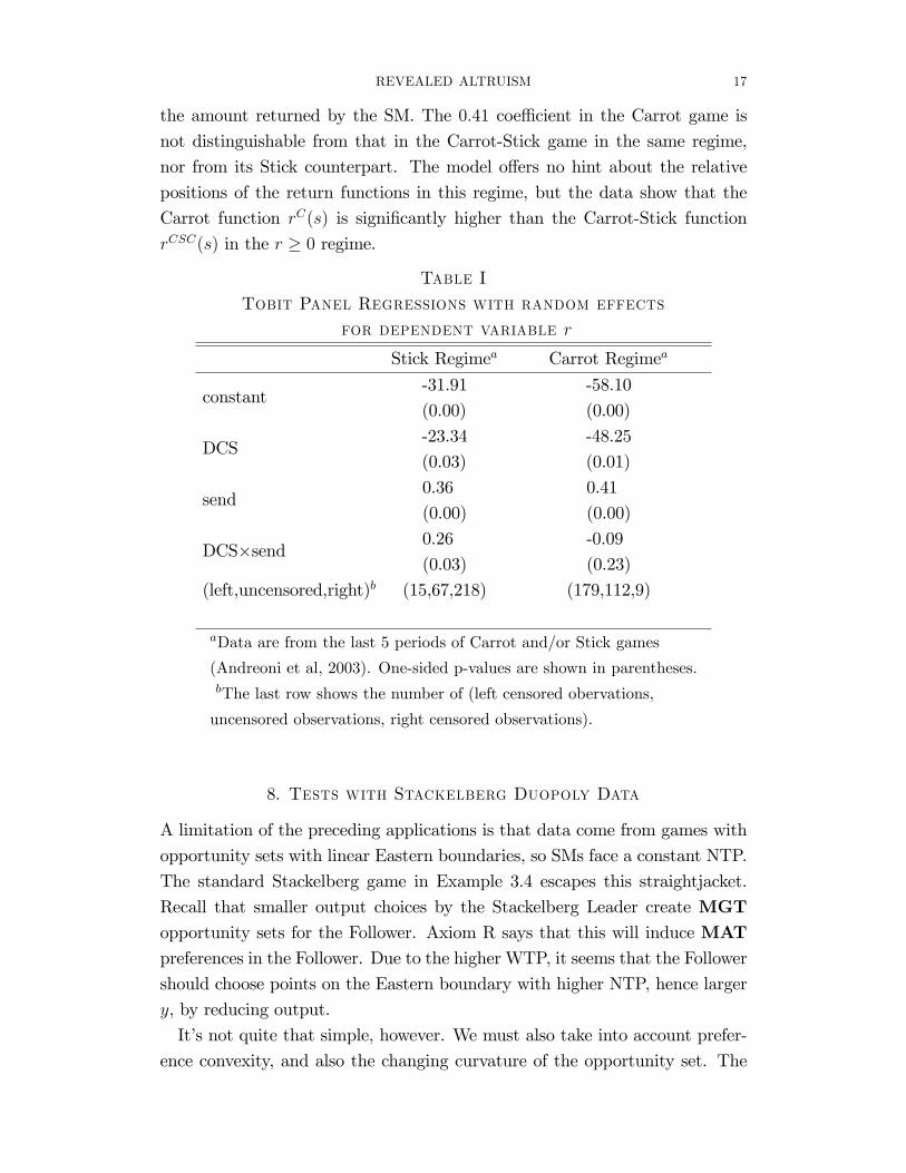
The table reports similar results for the Carrot regime. Again as predicted,
the amount sent s by the FM has a signi�cantly positive marginal impact on
5Spot checks indicate no substantial changes in results when all 10 periods are included.
REVEALED ALTRUISM 17
the amount returned by the SM. The 0:41 coe¢ cient in the Carrot game is
not distinguishable from that in the Carrot-Stick game in the same regime,
nor from its Stick counterpart. The model o¤ers no hint about the relative
positions of the return functions in this regime, but the data show that the
Carrot function rC(s) is signi�cantly higher than the Carrot-Stick function
rCSC(s) in the r � 0 regime.
Table I
Tobit Panel Regressions with random effects
for dependent variable r
Stick Regimea Carrot Regimea
constant-31.91
(0.00)
-58.10
(0.00)
DCS-23.34
(0.03)
-48.25
(0.01)
send0.36
(0.00)
0.41
(0.00)
DCS�send 0.26
(0.03)
-0.09
(0.23)
(left,uncensored,right)b (15,67,218) (179,112,9)
aData are from the last 5 periods of Carrot and/or Stick games
(Andreoni et al, 2003). One-sided p-values are shown in parentheses.bThe last row shows the number of (left censored obervations,
uncensored observations, right censored observations).
8. Tests with Stackelberg Duopoly Data
A limitation of the preceding applications is that data come from games with
opportunity sets with linear Eastern boundaries, so SMs face a constant NTP.
The standard Stackelberg game in Example 3.4 escapes this straightjacket.
Recall that smaller output choices by the Stackelberg Leader create MGT
opportunity sets for the Follower. Axiom R says that this will induce MAT
preferences in the Follower. Due to the higher WTP, it seems that the Follower
should choose points on the Eastern boundary with higher NTP, hence larger
y, by reducing output.
It�s not quite that simple, however. We must also take into account prefer-
ence convexity, and also the changing curvature of the opportunity set. The
18 BY JAMES C. COX, DANIEL FRIEDMAN, AND VJOLLCA SADIRAJ
next proposition sorts out these e¤ects and expresses them in terms of the Fol-
lower�s deviation from sel�sh best reply (the prediction of standard duopoly
theory).
Proposition 6. In the Stackelberg game of Example 3.4 let QD(qL) = qF � qoFbe the deviation of the Follower�s output choice qF from the sel�sh best reply
qoF = 12� 12qL when the Leader chooses output qL. One has
dQDdqL
= �12w � dw
dqLqL
where w = WTP (MqF ;MqL) is willingness to pay at the chosen point. Fur-
thermore,
(1) If Follower�s preferences A are �xed and linear, then w is constant withrespect to qL and
dQDdqL
is positive if and only if preferences at the chosen
point are malevolent.
(2) If Follower�s preferences A are �xed, satisfy IB and w � 1, then w isdecreasing in qL and
dQDdqL
contains an additional positive term.
(3) If Follower�s preferences satisfy Axiom R strictly, then w is decreasing
in qL anddQrDdqL
contains an additional positive term.
(4) If Follower�s preferences satisfy Axiom S strictly, then w is decreasing
in qL anddQsDdqL
has an additional positive (negative) term if the status
quo is smaller (larger) than qL:
Proposition 6 shows that an increase in qL has three di¤erent e¤ects:
- A reciprocity e¤ect, items (3) - (4) in the Proposition. If Axiom R holds
strictly, then the less generous opportunity set decreases the Follower�s WTP,
increasing qF and qD = QD(qL). Axiom S moderates or intensi�es this e¤ect,
depending on the status quo.
- A preference convexity (or substitution) e¤ect, item (2) in the Proposition.
The choice point is pushed west, where WTP is less, again increasing qD.
- An opportunity set shape e¤ect (in some ways analagous to an income
e¤ect), item (1) in the Proposition. The curvature of the parabola decreases.
Holding w =WTP constant, qD increases when the Follower is malevolent
(w < 0, hence qD > 0), and decreases when the Follower is benevolent (w > 0,
hence qD < 0).
A parametric example may clarify the logic. For given qL 2 [0; 24], the
Follower�s choice set is the parabola f(m; y) : m = MqF ; y = MqL;M = 24�qL�qF ; qF 2 [0; 24�qL]g, with NTP= �dm=dqF
dy=dqF= 24�qL�2qF
qL: Suppose that the
Follower has �xed Cobb-Douglas preferences represented by u(m; y) = my�,
REVEALED ALTRUISM 19
so WTP is �m=y = �qF=qL. Solving NTP=WTP, one obtains qF = Q(qLj�) =(24 � qL)=(2 + �): Noting that the sel�sh best reply is qoF = Q(qLj0); oneobtains a closed form expression for the deviation, qD = � �
4+2�(24� qL). For
�xed � positive (benevolent preferences) or smaller than �2 (pathologicallymalevolent preferences), the deviation is negative but increasing in the Leader�s
output; the opposite is true when � is negative but larger than �2 (moderatelymalevolent). This is the combined impact of the convexity (or substitution)
and shape (or income) e¤ects noted above. Of course, reciprocity e¤ects will
decrease � and hence increase qD.
We test predictions obtained from Proposition 6 on the Stackelberg duopoly
data of Huck, Müller, and Normann (2001, henceforth HMN). The parame-
ters are exactly as in Example 3.4 with integer output choices. The data
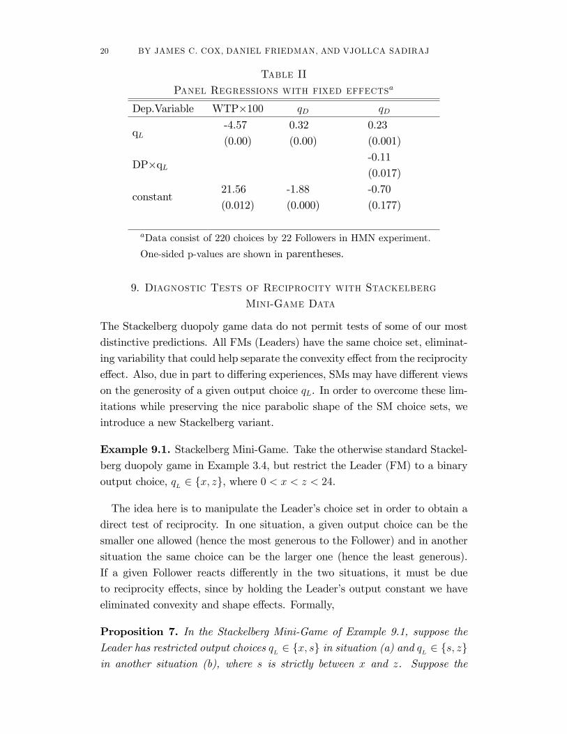
consist of 220 output pairs (qL; qF ) by 22 FMs (or Leaders) choosing qL 2f3; 4; 5; : : : ; 15g randomly rematched for 10 periods each with 22 SMs (orFollowers) who choose qF 2 f3; 4; 5; : : : ; 15g. The WTP can be inferred at achosen point (qL; qF ) by the NTP at that point, (24� 2qF � qL)=qL.Table II reports the test results. All observations reveal w � 1; as assumed
in Proposition 6. To check for asymmetric responses to large and small FM
choices (relative to the Cournot choice qL = 8), we de�ne the dummy vari-
able DP = 1 if qL � 8. All columns in the table report panel regressions
with individual subject �xed e¤ects. The �rst column, with dependent vari-
able WTP�100, �rmly rejects the hypothesis of benevolent linear and �xedpreferences: the coe¢ cient for qL is signi�cantly negative, not positive. In
view of part 1 of the Proposition, the second column, with dependent variable
QD, con�rms this result. We infer that QD is an increasing function of FM
output qL, consistent with convexity and reciprocity, in view of parts 2 and 3
of the Proposition. The last column reports that there is a stronger response
to �greedy�FM choices in excess of the Cournot output 8 than to �generous�
FM choices below or equal to output 8.
20 BY JAMES C. COX, DANIEL FRIEDMAN, AND VJOLLCA SADIRAJ
Table II
Panel Regressions with fixed effectsa
Dep.Variable WTP�100 qD qD
qL-4.57
(0.00)
0.32
(0.00)
0.23
(0.001)
DP�qL-0.11
(0.017)
constant21.56
(0.012)
-1.88
(0.000)
-0.70
(0.177)
aData consist of 220 choices by 22 Followers in HMN experiment.
One-sided p-values are shown in parentheses.
9. Diagnostic Tests of Reciprocity with Stackelberg
Mini-Game Data
The Stackelberg duopoly game data do not permit tests of some of our most
distinctive predictions. All FMs (Leaders) have the same choice set, eliminat-
ing variability that could help separate the convexity e¤ect from the reciprocity
e¤ect. Also, due in part to di¤ering experiences, SMs may have di¤erent views
on the generosity of a given output choice qL. In order to overcome these lim-
itations while preserving the nice parabolic shape of the SM choice sets, we
introduce a new Stackelberg variant.
Example 9.1. Stackelberg Mini-Game. Take the otherwise standard Stackel-berg duopoly game in Example 3.4, but restrict the Leader (FM) to a binary
output choice, qL2 fx; zg, where 0 < x < z < 24.
The idea here is to manipulate the Leader�s choice set in order to obtain a
direct test of reciprocity. In one situation, a given output choice can be the
smaller one allowed (hence the most generous to the Follower) and in another
situation the same choice can be the larger one (hence the least generous).
If a given Follower reacts di¤erently in the two situations, it must be due
to reciprocity e¤ects, since by holding the Leader�s output constant we have
eliminated convexity and shape e¤ects. Formally,
Proposition 7. In the Stackelberg Mini-Game of Example 9.1, suppose theLeader has restricted output choices q
L2 fx; sg in situation (a) and q
L2 fs; zg
in another situation (b), where s is strictly between x and z. Suppose the
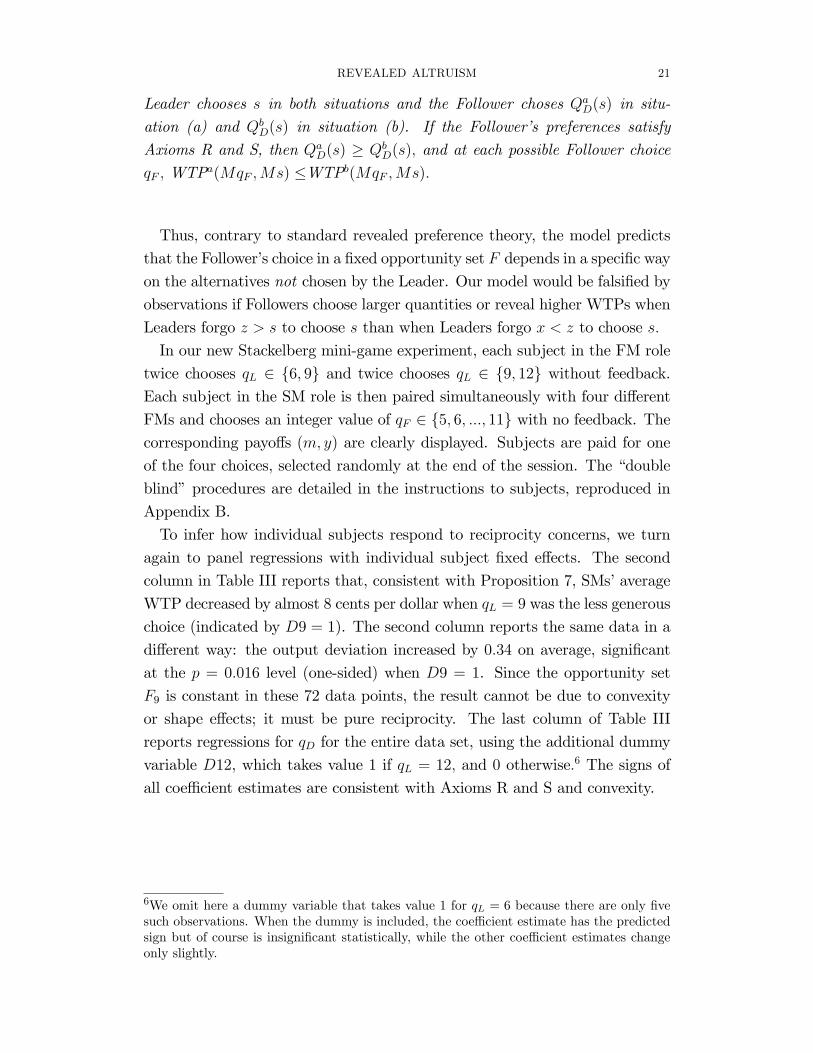
REVEALED ALTRUISM 21
Leader chooses s in both situations and the Follower choses QaD(s) in situ-
ation (a) and QbD(s) in situation (b). If the Follower�s preferences satisfy
Axioms R and S, then QaD(s) � QbD(s); and at each possible Follower choice
qF ; WTPa(MqF ;Ms) �WTPb(MqF ;Ms):
Thus, contrary to standard revealed preference theory, the model predicts
that the Follower�s choice in a �xed opportunity set F depends in a speci�c way
on the alternatives not chosen by the Leader. Our model would be falsi�ed by
observations if Followers choose larger quantities or reveal higher WTPs when
Leaders forgo z > s to choose s than when Leaders forgo x < z to choose s:
In our new Stackelberg mini-game experiment, each subject in the FM role
twice chooses qL 2 f6; 9g and twice chooses qL 2 f9; 12g without feedback.Each subject in the SM role is then paired simultaneously with four di¤erent
FMs and chooses an integer value of qF 2 f5; 6; :::; 11g with no feedback. Thecorresponding payo¤s (m; y) are clearly displayed. Subjects are paid for one
of the four choices, selected randomly at the end of the session. The �double
blind�procedures are detailed in the instructions to subjects, reproduced in
Appendix B.
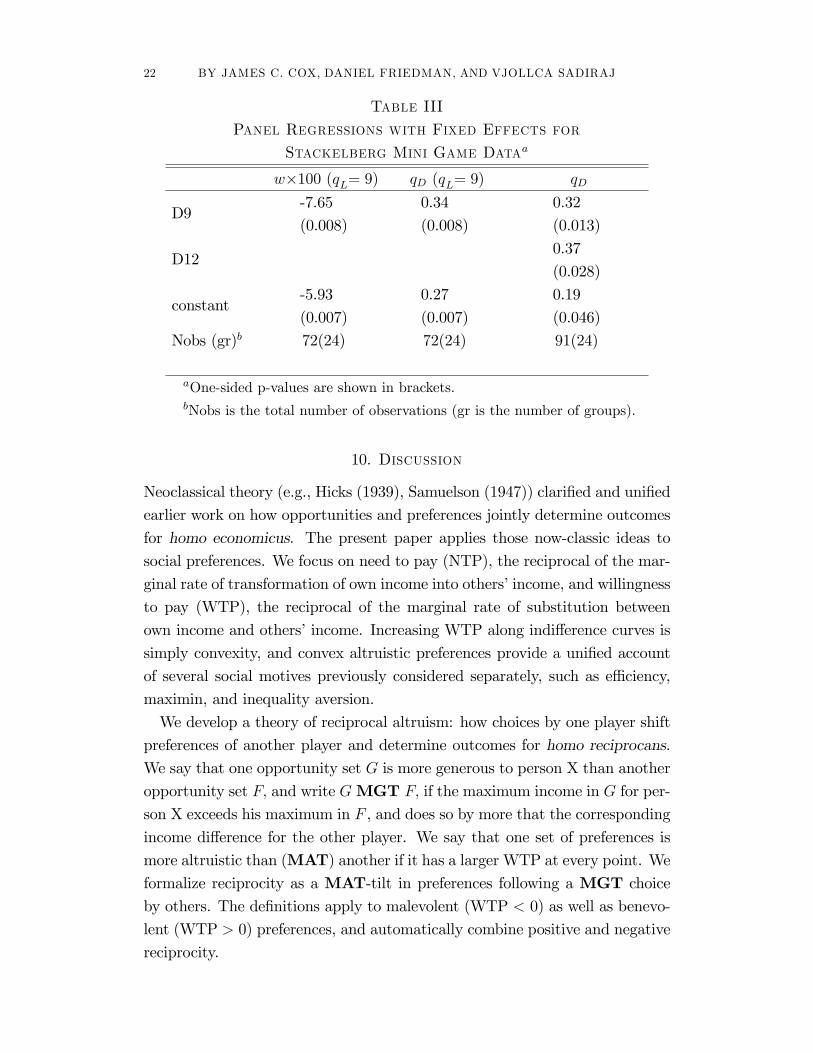
To infer how individual subjects respond to reciprocity concerns, we turn
again to panel regressions with individual subject �xed e¤ects. The second
column in Table III reports that, consistent with Proposition 7, SMs�average
WTP decreased by almost 8 cents per dollar when qL = 9 was the less generous
choice (indicated by D9 = 1). The second column reports the same data in a
di¤erent way: the output deviation increased by 0:34 on average, signi�cant
at the p = 0:016 level (one-sided) when D9 = 1. Since the opportunity set
F9 is constant in these 72 data points, the result cannot be due to convexity
or shape e¤ects; it must be pure reciprocity. The last column of Table III
reports regressions for qD for the entire data set, using the additional dummy
variable D12, which takes value 1 if qL = 12; and 0 otherwise:6 The signs of
all coe¢ cient estimates are consistent with Axioms R and S and convexity.
6We omit here a dummy variable that takes value 1 for qL = 6 because there are only �vesuch observations. When the dummy is included, the coe¢ cient estimate has the predictedsign but of course is insigni�cant statistically, while the other coe¢ cient estimates changeonly slightly.
22 BY JAMES C. COX, DANIEL FRIEDMAN, AND VJOLLCA SADIRAJ
Table III
Panel Regressions with Fixed Effects for
Stackelberg Mini Game Dataa
w�100 (qL= 9) qD (qL= 9) qD
D9-7.65
(0.008)
0.34
(0.008)
0.32
(0.013)
D120.37
(0.028)
constant-5.93
(0.007)
0.27
(0.007)
0.19
(0.046)
Nobs (gr)b 72(24) 72(24) 91(24)
aOne-sided p-values are shown in brackets.bNobs is the total number of observations (gr is the number of groups).
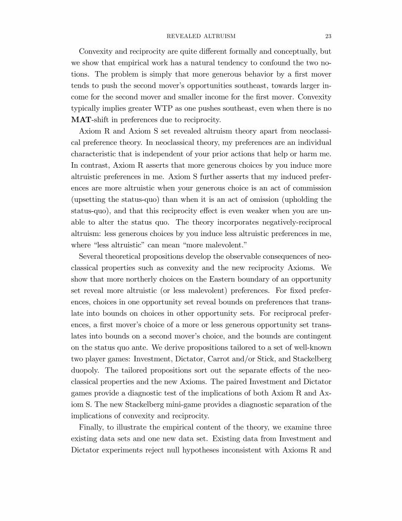
10. Discussion
Neoclassical theory (e.g., Hicks (1939), Samuelson (1947)) clari�ed and uni�ed
earlier work on how opportunities and preferences jointly determine outcomes
for homo economicus. The present paper applies those now-classic ideas to
social preferences. We focus on need to pay (NTP), the reciprocal of the mar-
ginal rate of transformation of own income into others�income, and willingness
to pay (WTP), the reciprocal of the marginal rate of substitution between
own income and others�income. Increasing WTP along indi¤erence curves is
simply convexity, and convex altruistic preferences provide a uni�ed account
of several social motives previously considered separately, such as e¢ ciency,
maximin, and inequality aversion.
We develop a theory of reciprocal altruism: how choices by one player shift
preferences of another player and determine outcomes for homo reciprocans.
We say that one opportunity set G is more generous to person X than another
opportunity set F; and write GMGT F; if the maximum income in G for per-son X exceeds his maximum in F , and does so by more that the corresponding
income di¤erence for the other player. We say that one set of preferences is
more altruistic than (MAT) another if it has a larger WTP at every point. We
formalize reciprocity as a MAT-tilt in preferences following a MGT choice
by others. The de�nitions apply to malevolent (WTP < 0) as well as benevo-
lent (WTP > 0) preferences, and automatically combine positive and negative
reciprocity.
REVEALED ALTRUISM 23
Convexity and reciprocity are quite di¤erent formally and conceptually, but
we show that empirical work has a natural tendency to confound the two no-
tions. The problem is simply that more generous behavior by a �rst mover
tends to push the second mover�s opportunities southeast, towards larger in-
come for the second mover and smaller income for the �rst mover. Convexity
typically implies greater WTP as one pushes southeast, even when there is no
MAT-shift in preferences due to reciprocity.
Axiom R and Axiom S set revealed altruism theory apart from neoclassi-
cal preference theory. In neoclassical theory, my preferences are an individual
characteristic that is independent of your prior actions that help or harm me.
In contrast, Axiom R asserts that more generous choices by you induce more
altruistic preferences in me. Axiom S further asserts that my induced prefer-
ences are more altruistic when your generous choice is an act of commission
(upsetting the status-quo) than when it is an act of omission (upholding the
status-quo), and that this reciprocity e¤ect is even weaker when you are un-
able to alter the status quo. The theory incorporates negatively-reciprocal
altruism: less generous choices by you induce less altruistic preferences in me,
where �less altruistic�can mean �more malevolent.�
Several theoretical propositions develop the observable consequences of neo-
classical properties such as convexity and the new reciprocity Axioms. We
show that more northerly choices on the Eastern boundary of an opportunity
set reveal more altruistic (or less malevolent) preferences. For �xed prefer-
ences, choices in one opportunity set reveal bounds on preferences that trans-
late into bounds on choices in other opportunity sets. For reciprocal prefer-
ences, a �rst mover�s choice of a more or less generous opportunity set trans-
lates into bounds on a second mover�s choice, and the bounds are contingent
on the status quo ante. We derive propositions tailored to a set of well-known
two player games: Investment, Dictator, Carrot and/or Stick, and Stackelberg
duopoly. The tailored propositions sort out the separate e¤ects of the neo-
classical properties and the new Axioms. The paired Investment and Dictator
games provide a diagnostic test of the implications of both Axiom R and Ax-
iom S. The new Stackelberg mini-game provides a diagnostic separation of the
implications of convexity and reciprocity.
Finally, to illustrate the empirical content of the theory, we examine three
existing data sets and one new data set. Existing data from Investment and
Dictator experiments reject null hypotheses inconsistent with Axioms R and
24 BY JAMES C. COX, DANIEL FRIEDMAN, AND VJOLLCA SADIRAJ
S in favor of alternative hypotheses consistent with the Axioms (and con-
vexity). Existing data from the Stick game and the Carrot and Stick game
support implications of Axiom R (and convexity). Existing data from a Stack-
elberg duopoly experiment con�rm reciprocity/convexity e¤ects and suggest
a stronger negative response to greedy behavior than the positive response to
generous behavior. Data from a new experiment with the Stackelberg mini-
game con�rm that reciprocity has a signi�cant impact even when convexity
e¤ects are held constant. The Stackelberg mini-game brings out a novel feature
of the new theory: contrary to standard revealed preference theory, revealed
altruism theory explains how alternatives not chosen by another can a¤ect
one�s own choice.
Theoretical clari�cation sets the stage for further empirical work. One can
now re�ne earlier empirical studies that examine the combined e¤ects of al-
truism and reciprocity. Such work should shed light not only on the extent to
which typical human preferences depart from sel�shness but also on the extent
to which such departures are altered by experiencing generous or ungenerous
behavior.
Further theoretical work is also in order. We consider two versions of the
�more generous than�relation but yet other versions may have implications
that are stronger (or just di¤erent). For example, generosity might be de�ned
in terms of players�utilities rather than in terms of material payo¤s (although
this would compromise observability). Other open theoretical questions con-
cern Axiom S, which invokes the status quo to distinguish between acts of
commission and omission, and between generous and greedy acts. But what
does it take for a particular act to become generally recognized as the sta-
tus quo? What if an act has bene�cial short run impact but is harmful in
the long run? Answers to these and other questions await further theoretical
development.
Department of Economics and Experimental Economics Center (ExCEN),
Andrew Young School of Policy Studies, Georgia State University, P.O. Box
3992, Atlanta, GA 30302-3992, U.S.A.; [email protected],
Department of Economics, 417 Building E2, University of California, Santa
Cruz, CA 95064, U.S.A.; [email protected],
and
REVEALED ALTRUISM 25
Department of Economics and Experimental Economics Center (ExCEN),
Andrew Young School of Policy Studies, Georgia State University, P.O. Box
3992, Atlanta, GA 30302-3992, U.S.A.; [email protected].
Appendix A. Mathematical proofs and derivations
A.1. Properties of Preferences. Recall that preferences over bundles (m; y) 2<2+ are admissible if they can be represented by a twice continuously dif-
ferentiable (smooth) utility function u such that @u(m; y)=@m = um > 0;
8(m; y) 2 <2+ (m-monotone) and the set f(m; y) 2 <2+ : u(m; y) � cgis convex for all c 2 < (convex). Recall also that willingness to pay is
w = w(m; y) =WTP(m; y) = uy=um:
It will be helpful to express convexity in terms of the curvature of indi¤erence
curves. At a given point, curvature has absolute value jKj = 1=R, where R
is the radius of the circle that is second-order tangent to the curve at the
given point. Let � denote the angle of the tangent to the indi¤erence curve
with the negative y-direction. The signed curvature is K = d�=ds where
s(t) =R t0
pm02(x) + y02(x)dx is arclength along the indi¤erence curve (e.g.,
Protter and Morrey, (1963, p. 394)).
Preferences are positively monotonic in m; hence upper contour sets are on
the right of indi¤erence curves in (m; y) space. The convexity of upper contour
sets implies that w decreases as we move up along the indi¤erence curve. The
�rst lemma veri�es this intuition and obtains other useful characterizations.
Lemma A.1. The following properties are equivalent for smooth m-monotonepreferences on <2+:(a) They are convex.
(b) Their indi¤erence curves everywhere have negative (or zero) curvature.
(c) wmw � wy � 0:
Proof: Note that along the indi¤erence curve � = arctan(dm=dy) =
arctan(�w): Into the de�nition K = d�=ds, insert d� = �d(w)=(1 + w2),ds =
pdm2 + dy2 and (holding u constant) �dm=dy = w to get
(A.1) K =1
pw2 + 1
3
dw
dy:
Since the expression inside the radical is positive, the sign of K is that of dwdy:
The upper contour set at a point (mo; yo) with u(mo; yo) = c lies on the right
or on the tangent hyperplane if and only if (dw=dy)ju(m;y)=c � 0, as can be
seen, e.g., from a straightforward adaptation of Protter and Morrey (1963).
26 BY JAMES C. COX, DANIEL FRIEDMAN, AND VJOLLCA SADIRAJ
Hence conditions (a) and (b) are equivalent. To verify the equivalence of (b)
and (c), simply substitute dw=dy = wmdm=dy + wy and dm=dy = �w into
(A.1) to obtain
(A.2) K = �wwm � wypw2 + 1
3 :
Q.E.D.
Lemma A.2. (d(NTP )=dy)j(m;y)2@F � 0 at every regular boundary point of
an opportunity set.
Proof: The reasoning is the same as in the previous Lemma. Along the
boundary
(A.3) K =1
pNTP 2 + 1
3
d(NTP )
dy:
Thus K = d�=ds has the same sign as d(NTP )=dy: Our feasible opportunity
set F lies on the left or on the tangent hyperplane at a point from the boundary
@F: Hence, as y increases the boundary is turning left, so � increases and (by
A.3) NTP increases.
Q.E.D.
The next Lemma characterizes homotheticity in order to facilitate comparisons
to the weaker properties used in the Propositions.
Lemma A.3. The following are equivalent:(a) Preferences are homothetic on <2+.(b) w =WTP is constant along every ray Rr = f(t; tr) : t > 0g � <2+:(c) wm + wyr = 0 along every ray Rr, r > 0.
Proof: By de�nition, preferences are homothetic if and only if they can
be represented by a utility function u(m; y) whose ratio of partial derivatives
um=uy depends only on the ratio m=y (e.g., Simon and Blume (1994, p. 503)).
Thus condition (a) implies that w = uy=um is constant along the ray with
r = m=y and so condition (b) must hold. In turn, condition (b) implies that
along that ray 0 = dw=dt = wmdm=dt + wydy=dt = wm + wyr, establishing
condition (c). Since rays with r > 0 foliate <2+ n (0; 0); condition (c) impliesthat w and hence um=uy depend only on r = m=y; i.e., (a) must hold.
Q.E.D.
REVEALED ALTRUISM 27
De�nition 3. Preferences are rather malevolent (resp. not very malevolent)on a domain D if w � wy=wm (resp. w � wy=wm) holds at all points in
D � <2+.
Lemma A.4. (a) If admissible preferences are homothetic on <2+ then theyare IB.
(b) Convexity on <2+ is equivalent to IB for preferences that are not very malev-olent, and is equivalent to wm � 0 for preferences that are rather malevolent.
Proof: For part a we need to show that wm(m; y) is non-negative. It
su¢ cies to show that the sign of w(m+ �; y)�w(m; y) is the same as the signof �, for all �. If � > 0 then (m + �; y) is on a ray (Ry=(m+�)) with a smaller
slope than the ray through (m; y): This, convexity and homotheticity imply
that w(m+�; y) � w(m; y). Similarly, w(m+�; y) � w(m; y) for negative �: Forpart b, recall from Lemma A.1 that convexity is equivalent to wmw�wy � 0:But this is equivalent to wm � 0 (wm � 0) if w � wy=wm (w � wy=wm):
Q.E.D.
To see the bite of the assumptions, consider preferences represented by u(m; y) =
mr=r � y(1+r)=(1 + r). For r > 1 these preferences are IB but neither convexnor homothetic. For r 2 (0; 1), however, they are convex but neither IB norhomothetic.
A.2. Proof that MAT is a Partial Ordering. The properties of re�exivityand transitivity are inherited from the re�exivity and transitivity of the real
ordering �. The antisymmetry property follows from Hicks�Lemma (Hicks
(1939, Appendix)): if preferences have the same MRS (or WTP) everywhere
in a domain D then they are the same on that domain.
Q.E.D.
A.3. Proof that MGT is a Partial Ordering. Re�exivity, antisymmetryand transitivity all are inherited from the corresponding properties of the real
ordering �.
Q.E.D.
28 BY JAMES C. COX, DANIEL FRIEDMAN, AND VJOLLCA SADIRAJ
A.4. Proof that Stackelberg Follower�s opportunity sets are MGT-ranked. The Follower�s opportunity set FqL has Eastern boundary f(m; y) :m = Mq
F; y = Mq
L; q
F2 [0; T � q
L]g where M = T � qL � qF : Along this
boundary NTP is given by
NTP = �dm=dqFdy=dqF
=T � q
L� 2q
F
qL
:
Note that NTP varies smoothly from positive to negative values as increasing
qFpasses through qo
F= T=2 � q
L=2, the sel�sh best response. To see that
a smaller output by the Leader produces a MGT opportunity set for the
Follower, �rst note that y�F (qL) = (T � qL)qL is obtained when qF = 0 and thatm�F (qL)
= 14(T � qL)2 is obtained from the standard (sel�sh) reaction function
qoF: To verify condition (a) in the MGT de�nition, let q
0L 2 (qL; T � qL) and
note that m�F (qL)
� m�F (q
0L)= 1
4(2T � qL � q
0L)(q
0L � qL) > 0. Condition (b)
follows from y�F (qL) � y�F (q0L)
= (qL + q0L � T )(q
0L � qL) � 0:
Q.E.D.
A.5. Examples of MGT-ordered Opportunity Sets.
Example A.5. Ring test (Liebrand (1984); see also (Sonnemans, van Dijkand van Winden (2005)). Let F (R) =
�(m; y) 2 <2+ : m2 + y2 � R2
for given
R > 0: On the circular part of the boundary, NTP is y=m and the curvature
is 1=R: Straightforwardly, F (R) MGT F (R0) if R > R
0:
Example A.6. Ultimatum game (Güth, Schmittberger, and Schwarze (1982)).The responder�s opportunities in the $10 ultimatum game consist of the origin
(0; 0) and (due to our free disposal assumption) the horizontal line segment
from (0; 10� x) to (x; 10� x). This set is not convex so it doesn�t qualify asan opportunity set by our de�nition. Its convex hull, however, is the opportu-
nity set in the Convex Ultimatum game (Andreoni, Castillo and Petrie (2003),
which is identical to that of the Power to Take game in the following example.
Example A.7. Power to Take game (Bosman and van Winden (2002)). The�take authority� player chooses a take rate b 2 [0; 1]. Then the responder
with income I chooses a destruction rate 1 � �. The resulting payo¤s arem = (1 � b)�I for the responder and y = b�I for the take authority. Thus,
with free disposal the responder�s opportunity set is the convex hull of three
points (m; y) = (0; 0); (0; bI) and ((1 � b)I; bI): Along the Eastern boundaryNTP is constant at (b�1)=b and the curvature is 0: To verify the strictMGT
REVEALED ALTRUISM 29
ranking, let b0> b � 0 produce SM opportunity sets F and G respectively, so
m�F = (1 � b
0)I and y�F = b
0I: Then m�
G �m�F = (b
0 � b)I > 0 > (b � b0)I =y�G � y�F . The �rst inequality con�rms part a of the de�nition and the entirestring con�rms part b.
Example A.8. Ultimatummini-games (Gale, Binmore, and Samuelson (1995),Falk, Fehr and Fischbacher (2003)). In the notation of the previous example,
the FM in these games chooses between b = 0:8 and one other value, either
b = 0:5 in the 5/5 game, or b = 0:2 in the 2/8 game, or b = 0:8 in the 8/2
game, or b = 1:0 in the 10/0 game. The previous example shows that the
(convexi�ed) opportunity sets are MGT-ranked by decreasing b. Axiom R
suggests that the SM is more likely to choose (0; 0) (reject the ultimatum)
rather than ((1 � b)I; bI) (accept) when the FM�s choice of b was less gener-ous. Hence rejections of the b = 0:8 proposal should be more frequent when
the alternative was b = 0:5 or b = 0:2 rather than b = 1:0. Axiom S suggests
that the responses would be muted when the alternative was b = 0:8 (i.e., no
choice). The data are consistent with these predicitions; see Cox, Friedman
and Gjerstad (2007) for a detailed structural analysis.
Example A.9. Moonlighting game (Abbink, Irlenbusch, and Renner (2000)).In this variant of the investment game, the FM sends s 2 [�I=2; I] to SM, whoreceives g(s) = ks for positive s and g(s) = s for negative s. Then the second
mover transfers t 2 [(�I + s)=k; I + g(s)] resulting in non-negative payo¤sm = I + g(s) � jtj ; and y = I � s + t for positive t and y = I � s + kt fornegative t: The second mover�s opportunity set is the convex hull of the points
(m; y) = (0; 0); (I+g(s)�(I�s)=k; 0); (I+g(s); I�s); and (0; 2I+g(s)�jsj).The NTP along the boundary of the opportunity set is 1 above and �1=kbelow the t = 0 locus, is 0 along the y axis, and is1 along the m-axis. Again,
curvature at all regular boundary points is K = 0. It is straightforward to
verify that larger s produces higherMGT-ranking.
Example A.10. Gift exchange labor markets (Fehr, Kirchsteiger, and Riedl(1993)). The employer with initial endowment I o¤ers a wage W 2 [0; I] andthe worker then chooses an e¤ort level e 2 [0; 1] with a quadratic cost functionc(e). The �nal payo¤s are m = W � c(e) for the worker and y = I + ke�Wfor the employer, where the productivity parameter k = 10 in a typical game.
The worker�s opportunity set is similar to the second mover�s in the investment
game, except that the Northeastern boundary is a parabolic arc instead of a
straight line of slope �1. Along this Eastern boundary NTP is 2e and the
30 BY JAMES C. COX, DANIEL FRIEDMAN, AND VJOLLCA SADIRAJ
curvature is �1=5(4e2 + 1)3=2: Also, if the employer o¤ers a wage in excessof his endowment I then the opportunity set includes part of the quadrant
[m > 0 > y]. It is straightforward but a bit messy to extend the de�nition
of opportunity set to include such possibilities. Again, one can directly verify
that larger W produces higherMGT-ranking.
Example A.11. Sequential VCM public good game with two players (Varian
(1994)). Each player has initial endowment I. FM contributes c1 2 [0; I] tothe public good. SM observes c1 and then chooses his contribution c2 2 [0; I].Each unit contributed has a return of a 2 (0:5; 1], so the �nal payo¤s are m =
I+ac1�(1�a)c2 for SM and y = I+ac2�(1�a)c1 for FM. SM�s opportunityset is the convex hull of the four points (m; y) = (0; I� (1�a)c1); (I+ac1; I�(1�a)c1); (aI+ac1; (1+a)I�(1�a)c1) and (0; (1+a)I�(1�a)c1): Along thePareto frontier, NTP is constant at (1�a)=a: Once again, a larger contributionc1 createsMGT opportunities for the second mover.
A.6. Proof of Proposition 1. Suppose that (mA; yA) =2 @EF . Then by
de�nition of @EF there exists z > mA such that M = (z; yA) 2 F . Positivemonotonicity in own payo¤ implies that M is strictly preferred to (mA; yA),
contradicting the hypothesis that (mA; yA) is the A-preferred point in F:
Q.E.D.
A.7. Proof of Proposition 2 (Theoretical Predictions for Fixed Op-portunity Sets). By Lemma A.2, NTP increases as y increases along @EF .Part 1. Convexity of F and optimality of (mB; yB) imply that @EF (in-
cluding the part north of (mB; yB)) lies in the negative closed halfspace for
the tangent line, HB to the B�indi¤erence curve through (mB; yB): B MATA implies that the tangent line, HA of the A�indi¤erence curve through thesame point (mB; yB) is a clockwise rotation of HB: Hence, the @EF�pointsnorth of (mB; yB) are from the negative halfspace of HA and from convexity
of preferences A their A�indi¤erence curves are at lower levels than (mB; yB).
Therefore (mA; yA) must be south of (mB; yB).
Part 2. By hypothesis, X = (m; y) is south of (mB; yB) and north of
(mA; yA). Let wa and wb denote WTP functions for A and B preferences;
by admissibility the functions are continous. The desired conclusion is triv-
ial if wb(m; y) = wa(m; y) and Lemma A.2 rules out wb(m; y) < wa(m; y),
so suppose wb(m; y) > wa(m; y): To construct the desired preferences P, let
REVEALED ALTRUISM 31
wP (Y ) = kwb(Y ) + (1� k)wa(Y ) where
k =NTP (m; y)� wa(m; y)wb(m; y)� wa(m; y)
:
Since wP is continous on <2+, classic theorems assure the existence of a utilityfunction whose WTP is wP (Y ) (Hurewicz (1958, p. 7-10); see also Hurwicz
and Uzawa (1971)). Let P the preferences represented by this utility function.Since the hypothesis implies that 0 < k < 1, we have B MAT P MAT A.By construction, (m; y) is P-chosen since wP (m; y) =NTP(m; y):Part 3. Linear preferences with w approaching �1 (+1) yield choices
arbitrarily close to SF (NF ):
Q.E.D.
A.8. Proof of Proposition 3 (Theoretical Predictions for Di¤erentOpportunity Sets). Suppose that X is a regular point from @EF: Then
x =NTP(X) is unique. Let the NTP of points from @EG take values be-
tween [ �; �]: Z is: NF ; if NTP(X) > �; SF ; if NTP(X) < �; otherwise Z
is the point of @EG with x 2NTP(Z). Such a point exists by the IntermediateValue Theorem and is unique because G is convex. If X is not a regular point
then NTP(X) takes values from some [��; ��]: Make the arbitary convention
that x = �� and proceed as with a regular point.
Part 1. Follows from standard revealed preference theory (e.g., Varian
(1992, p. 131-133)).
Part 2. Clearly bm � mF and WTPm � 0 imply WTP (Y ) � WTP (X),
whileNTP@F (X) � NTP@G(Y ), optimality ofX (soWTP (X) = NTP@F (X))
and transitivity together imply that WTP (Y ) � NTP@G(Y ): By convexity ofA all points from @G north of Y are on lower A�indi¤erence curves than Y sothey cannot be W: Thus W must be south of Y , and 2a follows. One obtains
2b in just the same way.
Part 3. Suppose Z is southeast of X: Then
WTP (Z) � WTP (X) = NTP@F (X) = NTP@G(Z):
where the �rst inequality follows by assumption whereas the equalities follow
from optimality of X and by construction of Z. By convexity of A all points
from @G south of Z are on lower A�indi¤erence curves than Z so they cannotbe W: That is, W must be north of Z. Likewise for the case with Z northwest
of X.
Q.E.D.
32 BY JAMES C. COX, DANIEL FRIEDMAN, AND VJOLLCA SADIRAJ
A.9. Proof of Proposition 4 (Investment Game). Part 1. Let r(s) bethe optimal choice of SM when the FM choice is s and let XFs = (10 + 3s�r(s); 10� s+ r(s)). Let s0 > s. Proposition 3.2:b tells us that y
Fs0� y
Fs: This
implies that r(s0) � s0 � s+ r(s) > r(s):
Part 2. Applying Axiom R in the argument above, we see that r(s0) in-
creases more rapidly in s than for �xed preferences.
Part 3. Axiom S has the indicated impact since, as shown in the previous
subsection, Fs isMGT ordered by s.
Q.E.D.
A.10. Proof of Proposition 5 (Carrot, Stick and Carrot-Stick Games).Let r(s) be the optimal choice of SM when the FM choice is s and let
XFs = (s � jr(s)j ; 240 � s + 5r(s)). Let s0 > s. The amount return r(s)
is non-positive in the Stick Game, non-negative in the Carrot game and it can
be both in the Carrot-Stick game.
Part 1. Proposition 3.2:b tells us that yFs0� y
Fs: This implies that r(s
0) �
(s0 � s)=5 + r(s) > r(s).Part 2. Applying AxiomR in the argument above, we see that r(s) increases
more rapidly in s than for �xed preferences in the Stick game.
Q.E.D.
A.11. Proof of Proposition 6 (Stackelberg Duopoly Game). The FOCcan be written as w(qF ; qL) �WTP(MqF ;MqL) =NTP= (24 � 2qF )=qL � 1,which can be rewritten as
(A.4) qF = 12�w(qF ; qL) + 1
2qL:
Inserting the de�nition of QD from the statement of the proposition, we obtain
(A.5) QD = �w(qF ; qL)
2qL:
Part 1. Linear preferences. If Follower�s preferences are �xed and linear withWTP= w then di¤erentiation of (A.5) with respect to qL gives
dQDdqL
= �w2:

REVEALED ALTRUISM 33
Part 2. Convex Preferences. If Follower�s preferences are �xed and convexthen
dQDdqL
= �w(qF ; qL)2
� qL2
dw(qF ; qL)
dqLThe additional (second) term above is positive because, as we now will verify,
dw(qF ; qL)=dqL is negative. Indeed,
dw(qF ; qL)
dqL= wm
dm
dqL+ wy
dy
dqL
= wm((�1�dqFdqL
)qF +MdqFdqL
) + wy((�1�dqFdqL
)qL +M)
which after substituting M = 24 � qL � qF ; qF = 12 � (w(qF ; qL) + 1)qL=2and dqF=dqL = �(w(qF ; qL) + 1)=2 � (dw(qF ; qL)=dqL)qL=2 and solving fordw(qF ; qL)=dqL we get
dw(qF ; qL)
dqL=B
A
where
A = 2 + [wmw � wy] q2L > 0by Lemma (A.1), and
B = 24(wy � wm) + qL(1� w)(wm � wy + wwm � wy)
= (wy � wm)(24� qL(1� w)) + qL(1� w)(wwm � wy)
Note that qF � 24� qL and (A.4) imply that the sign of the second factor inthe �rst term is positive; hence B is negative if and only if
wy � wmwwm � wy
� 1� w24=qL � (1� w)
The current assumptions of w � 1, convexity and IB (i.e. wm � 0) ensure thatthe right-hand-side of the last expression is non-negative whereas left-hand
side is negative, so the inequality holds.
Part 3. Axiom R E¤ect. Let wr(qF ; qL) denote WTP for changed prefer-
ences as per Axiom R. Then
QrD = �wr(qF ; qL)
2qL
for all qL; and
dQrDdqL
= �wr(qF ; qL)
2� qL2
dwr(qF ; qL)
dqL
= �w(qF ; qL)2
� wr(qF ; qL)� w(qF ; qL)
2� qL2
dwr(qF ; qL)
dqL:
34 BY JAMES C. COX, DANIEL FRIEDMAN, AND VJOLLCA SADIRAJ
From Axiom R the second term is positive and similarly as in part 2 for the
sign of the third term.
Part 4. Axiom S E¤ect. Let ws(qF ; qL) denote WTP for changed prefer-
ences as in Axiom S. Then
QcD = �ws(qF ; qL)
2qL
is smaller (larger) than QrD if the status quo is smaller (larger) than qL, and
dQsDdqL
= �ws(qF ; qL)
2� qL2
dws(qF ; qL)
dqL
has an additional positive (negative) term if the status quo is smaller (larger)
than qL:
Q.E.D.
A.12. Proof of Proposition 7 (Stackelberg Mini-Game). In situation(a) induced preferences AaFs are AaF cs or A
aF �sdepending on whether output x
is considered as status quo by the Follower. Axiom S implies AaF os MAT AaF cs
and AaF os MAT AaF �s . Similarly, in situation (b) Axiom S implies AbF cs MATAF os and AbF �s MAT AF os : By transitivity AbFs MAT AaFs : Then the the lastinequality is straightforward by de�nition of MAT whereas for the �rst one
recall that: (i) qoF stays constant (it depends only on s), and NTP along @Fsdecreases as qF increases.
Q.E.D.
Appendix B. Instructions
WelcomeThis is an experiment about decision-making. You will be paid a $5 partici-
pation fee plus an additional positive or zero amount of money determined by
the decisions that you and the other participants make, as explained below.
Payment is in cash at the end of the experiment. A research foundation has
provided the funds for this experiment.
No Talking AllowedNow that the experiment has begun, we ask that you do not talk. If you have
a question, please raise your hand and an experimenter will approach you and
answer your question in private.
A Monitor and Two Groups
REVEALED ALTRUISM 35
A monitor will be selected randomly from among those of you who came here
today. The rest of you have been divided randomly into two groups, called the
First Mover Group and the Second Mover Group.
Complete PrivacyThe experiment is structured so that no one � not even the experimenters,
the monitor, and the other subjects � will ever know your personal decision
in the experiment. You collect your cash payment from a sta¤ person in the
Economics Department o¢ ce who has no other role in the experiment. Your
payment is in a sealed envelope with a code letter (A, B, C, etc). Your privacy
is guaranteed because neither your name nor your student ID number will
appear on any decision records. The only identifying mark on the decision
forms will be a code letter known only to you. You will show your code letter
to the sta¤ person and nobody else will see it. The experimenters will not be
in the department o¢ ce when you collect you cash payment. This procedure
is used to protect your privacy.
The Idea of the GameThe game involves two players, called the First Mover (FM) and the Second
Mover (SM), in the roles of producers of an identical good. Each decides how
much to produce. The pro�t for each player is the number of units he decides
to produce times price, net of cost. The price of the good decreases as total
production increases. If you and the other player produce too much, you will
drive down the price and your pro�ts. Of course, if you don�t produce much
you won�t have many units to sell.
To simplify your task, the pro�ts will be calculated for you and shown in an
easy-to-read table. Your cash payment will include the pro�t you earn in one
round of the game. The round will be selected randomly at the end of the
experiment.
Game DetailsEach round the FM chooses between two possible amounts to produce, as
shown in a table with two rows. The SM sees the choice of the FM, and then
decides among seven possible amounts to produce, as shown in seven columns
of the same table. The table shows the pro�ts for both players. The FM�s
pro�t is shown in italics in the lower left corner of each box, and the SM�s
pro�t is shown in bold in the upper right corner. For example, in Table B.I
below, if FM chooses Output=6 and SM then chooses Output=4, then FM�s
pro�t is 84 and SM�s pro�t is 56.

36 BY JAMES C. COX, DANIEL FRIEDMAN, AND VJOLLCA SADIRAJ
Table B.I
SM�s Choice of Output Quantity:4 5 6 7 8 9 10 11
FM�s Output=6 8456
7865
7272
6677
6080
5481
4880
4277
FM�s Output=9 9944
9050
8154
7256
6356
5454
4550
3644
Di¤erent Subject Pairs in Every DecisionEach First Mover and each Second Mover will make four decisions. But the
pairing of First Movers with Second Movers will be di¤erent in every decision.
This means that you will interact with a DIFFERENT person in the other
group in every decision that you make.
Experiment Procedures and the MonitorAt the beginning of the experiment, the monitor will walk through the room
carrying a box containing unmarked, large manila envelopes. Each subject in
the First Mover Group will take one of these envelopes from the box. This
envelope will contain the experiment decision forms and a code letter.
After the First Movers have made their decisions, they return the experiment
decision forms to their large manila envelopes and then walk to the front of the
room and deposit the envelopes in the box on the table. It is very important
that the First Movers do NOT return their code letters to the large manila
envelopes, because they will need them to collect their payo¤s.
After all First Movers have deposited their envelopes in the box, the Monitor
will take the box to another room in which the experimenters will sort the
decision forms and place them in the correct large manila envelopes for the
Second Movers. The experimenters will also put code letters in the envelopes
for the Second Movers.
Next, the Monitor will walk through the room carrying a box containing un-
marked, large manila envelopes. Each subject in the Second Mover Group
will take one of these envelopes from the box. This envelope will contain the
experiment decision forms and a code letter.
After the Second Movers have made their decisions, they return the experiment
decision forms to their large manila envelopes and then walk to the front of the
room and deposit the envelopes in the box on the table. It is very important
that the Second Movers do NOT return their code letters in the large manila
envelopes because they will need them to collect their payo¤s.
After all Second Movers have deposited their envelopes in the box, the Monitor
will take the box to another room in which the experimenters will record the
pro�ts and cash payments determined by the subjects�decisions.

REVEALED ALTRUISM 37
A Roll of a Die Determines Which Decision Pays MoneyAlthough you will make four decisions, only one will pay cash. Which of these
decisions will pay cash will be determined by rolling a six-sided die. The
experimenter will roll the die in front of you and the monitor will announce
which of the numbered sides has ended up on top. The �rst number from 1
to 4 that ends up on top will determine the page number of the decision that
pays cash.
The monitor�s cash payment will be the average of all First Movers and Second
Movers payments.
Be CarefulBe careful in recording your decisions. If a First Mover forgets to circle one of
the rows in the table, or circles both rows on the same decision page, then it
will be impossible to ascertain what decision the First Mover made. In that
case, the First Mover will get paid 0 and the Second Mover will get paid 60
if that decision page is selected for payo¤ by the roll of the die. If a Second
Mover doesn�t circle a column, then it will be impossible to ascertain what
decision the Second Mover made. In that case, the Second Mover will get paid
0 and the First Mover will get paid 60 if that decision page is selected for
payo¤ by the roll of the die.
Pay RatesFor each point of pro�t you earn, the experimenter will put a �xed number
of dollars in your envelope. This �xed number is called the pay rate and is
written on the board at the front of the room. Today�s pay rate is $0.25, which
means that every participant earns 25 cents for each pro�t point shown in the
table.
Frequently Asked QuestionsQ1: Exactly how are pro�ts calculated in the Tables?
A: Price is 30 minus the sum of FM output and SM output. Marginal cost is
6. Pro�t is output times (price minus marginal cost). But you don�t have to
worry about doing the calculation; the Tables do it for you.
Q2: Who will know what decisions I make?
A: Nobody else besides you; that is the point of the private envelopes etc. The
experimenters are only interested in knowing the distribution of choices for
FMs and SMs, not in the private decisions of individual participants.
Q3: Is this some psychology experiment with an agenda you haven�t told us?
A: No. It is an economics experiment. If we do anything deceptive, or don�t
pay you cash as described, then you can complain to the campus Human

38 BY JAMES C. COX, DANIEL FRIEDMAN, AND VJOLLCA SADIRAJ
Subjects Committee and we will be in serious trouble. These instructions are
on the level and our interest is in seeing the distribution of choices made in
complete privacy.
Any More Questions?If you have any questions, please raise your hand and an experimenter will
approach you and answer your question in private. Make sure that you under-
stand the instructions before beginning the experiment; otherwise you could,
by mistake, mark a di¤erent decision than you intended.
Quiz
(1) In Table B.II below, what are the two possible output choices for the
FM? __(2) Does the SM see the FM�s choice? (Y or N)
(3) In Table B.II, can the SM choose:
(a) Output=5? __(Y or N)
(b) Output =7?__(Y or N)
(c) Output=12?__(Y or N)
(4) Suppose the FM chooses the top row (Output = 9) in Table B.II and
the SM chooses a middle column (Output = 8).
(a) How many points will the FM get? __ points
(b) How much money is that if this is the decision that pays money?
$ __
(c) How much will the SM get in this case? __ points, $ __
(5) In the previous question, if SM chose Output=9 instead of Output=8,
(a) how many more or fewer points would the SM get?
__ more/fewer points
(b) how many more or fewer points would the FM get?
__ more/fewer points
(6) If the FM chooses the top row, what is the maximum number of points
that the SM can get? __ the minimum number?__(7) If the FM chooses the bottom row, what is the maximum number of
points that the SM can get? __ the minimum number?
(8) Will the SM ever be able to tell which person made any FM choice?
(Y or N)
(9) Will the FM ever be able to tell which person made any SM choice?
(Y or N)
(10) Will the experimenter ever be able to tell who made any choices?
(Y or N)
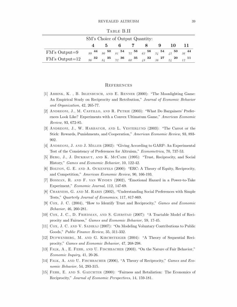
REVEALED ALTRUISM 39
Table B.II
SM�s Choice of Output Quantity:
4 5 6 7 8 9 10 11FM�s Output=9 99
4490
5081
5472
5663
5654
5445
5036
44
FM�s Output=12 9632
8435
7236
6035
4832
3627
2420
1211
References
[1] Abbink, K. , B. Irlenbusch, and E. Renner (2000): �The Moonlighting Game:
An Empirical Study on Reciprocity and Retribution,�Journal of Economic Behavior
and Organization, 42, 265-77.
[2] Andreoni, J., M. Castillo, and R. Petrie (2003): �What Do Bargainers�Prefer-
ences Look Like? Experiments with a Convex Ultimatum Game,�American Economic
Review, 93, 672-85.
[3] Andreoni, J., W. Harbaugh, and L. Vesterlund (2003): �The Carrot or the
Stick: Rewards, Punishments, and Cooperation,�American Economic Review, 93, 893-
902.
[4] Andreoni, J. and J. Miller (2002): �Giving According to GARP: An Experimental
Test of the Consistency of Preferences for Altruism,�Econometrica, 70, 737-53.
[5] Berg, J., J. Dickhaut, and K. McCabe (1995): �Trust, Reciprocity, and Social
History,�Games and Economic Behavior, 10, 122-42.
[6] Bolton, G. E. and A. Ockenfels (2000): �ERC: A Theory of Equity, Reciprocity,
and Competition,�American Economic Review, 90, 166-193.
[7] Bosman, R. and F. van Winden (2002), �Emotional Hazard in a Power-to-Take
Experiment,�Economic Journal, 112, 147-69.
[8] Charness, G. and M. Rabin (2002), �Understanding Social Preferences with Simple
Tests,�Quarterly Journal of Economics, 117, 817-869.
[9] Cox, J. C. (2004), �How to Identify Trust and Reciprocity,�Games and Economic
Behavior, 46, 260-281.
[10] Cox, J. C., D. Friedman, and S. Gjerstad (2007): �A Tractable Model of Reci-
procity and Fairness,�Games and Economic Behavior, 59, 17-45.
[11] Cox, J. C. and V. Sadiraj (2007): �On Modeling Voluntary Contributions to Public
Goods,�Public Finance Review, 35, 311-332.
[12] Dufwenberg, M. and G. Kirchsteiger (2004): �A Theory of Sequential Reci-
procity,�Games and Economic Behavior, 47, 268-298.
[13] Falk, A., E. Fehr, and U. Fischbacher (2003). �On the Nature of Fair Behavior,�
Economic Inquiry, 41, 20-26.
[14] Falk, A. and U. Fischbacher (2006), �A Theory of Reciprocity,�Games and Eco-
nomic Behavior, 54, 293-315.
[15] Fehr, E. and S. Gaechter (2000): �Fairness and Retaliation: The Economics of
Reciprocity,�Journal of Economic Perspectives, 14, 159-181.
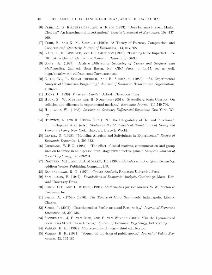
40 BY JAMES C. COX, DANIEL FRIEDMAN, AND VJOLLCA SADIRAJ
[16] Fehr, E., G. Kirchsteiger, and A. Riedl (1993): �Does Fairness Prevent Market
Clearing? An Experimental Investigation,�Quarterly Journal of Economics, 108, 437-
460.
[17] Fehr, E. and K. M. Schmidt (1999): �A Theory of Fairness, Competition, and
Cooperation,�Quarterly Journal of Economics, 114, 817-868.
[18] Gale, J., K. Binmore, and L. Samuelson (1995): �Learning to be Imperfect: The
Ultimatum Game,�Games and Economic Behavior, 8, 56-90
[19] Gray, A. (1997): Modern Di¤erential Geometry of Curves and Surfaces with
Mathematica, 2nd ed. Boca Raton, FL: CRC Press, p. 14-17. see as well,
http://mathworld.wolfram.com/Curvature.html.
[20] Guth, W., R. Schmittberger, and B. Schwarze (1982): �An Experimental
Analysis of Ultimatum Barga:ining,�Journal of Economic Behavior and Organization,
4, 367-88.
[21] Hicks, J. (1939). Value and Capital. Oxford: Clarendon Press.
[22] Huck, S., W. Muller and H. Normann (2001): �Stackelberg beats Cournot: On
collusion and e¢ ciency in experimental markets,�Economic Journal, 111,749-766.
[23] Hurewicz, W., (1958): Lectures on Ordinary Di¤erential Equations. New York: Wi-
ley.
[24] Hurwicz, L. and H. Uzawa (1971): �On the Integrability of Demand Functions,�
in J.S.Chipman et al. (eds.), Studies in the Mathematical Foundations of Utility and
Demand Theory. New York: Harcourt, Brace & World.
[25] Levine, D. (1998): �Modeling Altruism and Spitefulness in Experiments,�Review of
Economic Dynamics, 1, 593-622.
[26] Liebrand, W.B.G. (1984): �The e¤ect of social motives, communication and group
sizes on behavior in an n-preson multi stage mixed motive game,�European Journal of
Social Psychology, 14, 239-264.
[27] Protter, M.H. and C.B. Morrey, JR. (1963): Calculus with Analytical Geometry,
Addison-Wesley Publishing Company, INC.
[28] Rockafellar, R. T. (1970): Convex Analysis, Princeton University Press.
[29] Samuelson, P. (1947): Foundations of Economic Analysis. Cambridge, Mass., Har-
vard University Press.
[30] Simon, C.P. and L. Blume, (1994): Mathematics for Economists, W.W. Norton &
Company, Inc.
[31] Smith, A. <1759> (1976): The Theory of Moral Sentiments. Indianapolis, Liberty
Classics.
[32] Sobel, J. (2005): �Interdependent Preferences and Reciprocity,�Journal of Economic
Literature, 43, 392-436.
[33] Sonnemans, J, F. van Dijk, and F. van Winden (2005): �On the Dynamics of
Social Ties Structures in Groups,�Journal of Economic Psychology, forthcoming.
[34] Varian, H. R. (1992): Microeconomic Analysis, third ed., Norton.
[35] Varian, H. R. (1994): �Sequential provision of public goods,�Journal of Public Eco-
nomics, 53, 165-186.
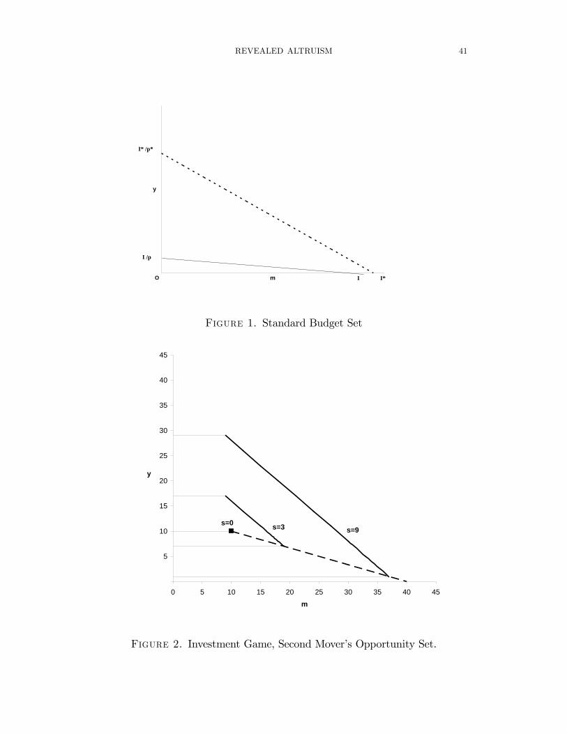
REVEALED ALTRUISM 41
m
y
I
I /p
O I*
I* /p*
Figure 1. Standard Budget Set
0
5
10
15
20
25
30
35
40
45
0 5 10 15 20 25 30 35 40 45
m
y
s=9s=3s=0
Figure 2. Investment Game, Second Mover�s Opportunity Set.
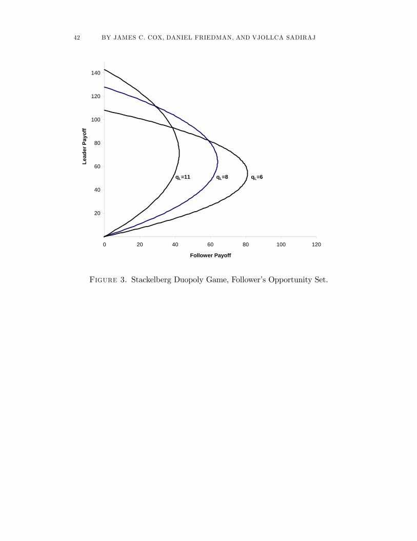
42 BY JAMES C. COX, DANIEL FRIEDMAN, AND VJOLLCA SADIRAJ
0
20
40
60
80
100
120
140
0 20 40 60 80 100 120
Follower Payoff
Lead
er P
ayof
f
qL=11 qL=8 qL=6
Figure 3. Stackelberg Duopoly Game, Follower�s Opportunity Set.
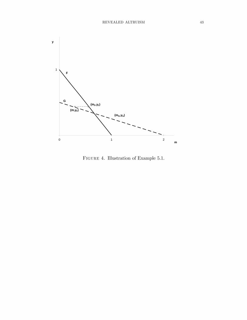
REVEALED ALTRUISM 43
0
1
0 1 2m
y
(mF,yF)
(m,yF)
F
G
(mG,yG)
Figure 4. Illustration of Example 5.1.
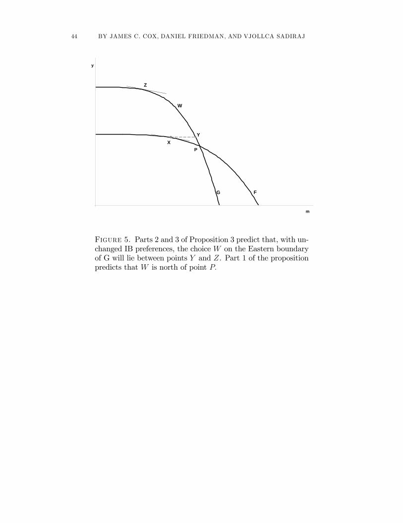
44 BY JAMES C. COX, DANIEL FRIEDMAN, AND VJOLLCA SADIRAJ
0.000.00 m
y
G F
XY
Z
W
P
Figure 5. Parts 2 and 3 of Proposition 3 predict that, with un-changed IB preferences, the choice W on the Eastern boundaryof G will lie between points Y and Z. Part 1 of the propositionpredicts that W is north of point P:
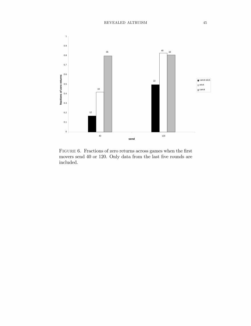
REVEALED ALTRUISM 45
0
0.1
0.2
0.3
0.4
0.5
0.6
0.7
0.8
0.9
1
40 120send
fract
ions
of z
ero
retu
rns
carrot-stick
stick
carrot
12
19
35
22
40 16
Figure 6. Fractions of zero returns across games when the �rstmovers send 40 or 120. Only data from the last �ve rounds areincluded.