TerraNNI: Natural Neighbor Interpolation on a 3D Grid Using aGPU∗

Alex BeutelSchool of Computer ScienceCarnegie Mellon University

abeutel@cs.cmu.edu

Thomas Mølhave, Pankaj K. AgarwalDepartment of Computer Science

Duke Universitythomasm,pankaj@cs.duke.edu

Arnold P. Boedihardjo, James A. ShineTopographic Engineering CenterU.S. Army Corps of Engineers

Arnold.p.boedihardjo,James.a.shine@usace.army.mil

ABSTRACTWith modern focus on LiDAR technology the amount of topo-graphic data, in the form of massive point clouds, has increaseddramatically. Furthermore, due to the popularity of LiDAR, re-peated surveys of the same areas are becoming more common.This trend will only increase as topographic changes prompt sur-veys over already scanned terrain, in which case we obtain largespatio-temporal data sets.

In dynamic terrains, such as coastal regions, such spatio-temporaldata can offer interesting insight into how the terrain changes overtime. An initial step in the analysis of such data is to create a digitalelevation model representing the terrain over time. In the case ofspatio-temporal data sets those models often represent elevation ona 3D volumetric grid. This involves interpolating the elevation ofLiDAR points on these grid points. In this paper we show how toefficiently perform natural neighbor interpolation over a 3D volu-metric grid. Using a graphics processing unit (GPU), we describedifferent algorithms to attain speed and GPU-memory trade-offs.Our algorithm extends to higher dimensions. Our experimental re-sults demonstrate that the algorithm is efficient and scalable.

Categories and Subject Descriptors: D.2 [Software]: SoftwareEngineering; F.2.2 [Nonnumerical Algorithms and Problems]: Ge-ometrical problems and computations; H.2.8 [Database Manage-ment]: Database Applications—Data Mining, Image Databases,Spatial Databases and GIS

General Terms: Performance, Algorithms

Keywords: LIDAR, Massive data, GIS, Natural Neighbor Interpo-lation∗This work is supported by NSF under grants CNS-05-40347, IIS-07-13498, CCF-09-40671, and CCF-1012254, by ARO grants W911NF-07- 1-0376 and W911NF-08-1-0452, by U.S. Army ERDC-TEC grant W9132V-11-C-0003, by NIH grant 1P50-GM-08183-01, and by a grant from theU.S.-Israel Binational Science Foundation..

Permission to make digital or hard copies of all or part of this work forpersonal or classroom use is granted without fee provided that copies arenot made or distributed for profit or commercial advantage and that copiesbear this notice and the full citation on the first page. To copy otherwise, torepublish, to post on servers or to redistribute to lists, requires prior specificpermission and/or a fee.ACM SIGSPATIAL GIS ’11 November 1-4, 2011. Chicago, IL, USACopyright 2011 ACM 978-1-4503-1031-4/11/11 ...$10.00.

1 IntroductionModern sensing and mapping technologies such as airborne LiDARtechnology can rapidly map the earth’s surface at 15-20cm horizon-tal resolution. Since LiDAR provides a relatively simple and cheapway of surveying large terrains, some areas are (or will be) sur-veyed multiple times, yielding large spatio-temporal data sets. Forexample, the coastal region of North Carolina has been mappedevery 1-2 years since the mid 1990’s[1]. Figure 1 shows a spatio-temporal model of a portion of this region constructed from the dataset. Such data sets provide tremendous opportunities for a widerange of commercial, scientific, and military applications. For in-stance, unmanned aerial vehicles can survey an area over a certaintime period and the resulting spatio-temporal topographic data canbe used to detect the location of new buildings, machinery, or veg-etation. On a larger scale, they can be used to offer interesting in-sights into understanding terrain dynamics. For example, there hasbeen much interest on studying the movement of sand dunes anderosion at the North Carolina coast [18]. It is essential for manyapplications to exploit the high-resolution data sets since small fea-tures may have a large impact on the output. For instance, it is vitalthat dikes and other features are present in data sets used for hydro-logical modeling, but these features are often relatively small andunlikely to disappear if the resolution is low [5, 19].

Capitalizing on the opportunities presented by high-resolutiondata sets and transforming massive amount of spatio-temporal to-pographic data into useful information requires that several algo-rithmic challenges be addressed. To begin with, the scattered pointset S generated by LiDAR cannot be used directly by many GIS al-gorithms. They instead operate on a digital elevation model (DEM).Because of its simplicity and efficiency, the most widely used DEMis a 2D uniform grid in which an elevation value is stored at eachcell. For spatio-temporal data, this translates into a 3D grid withtime representing the third dimension. One has to extend the ele-vation measured by LiDAR at the points of S via interpolation toa uniform grid Q ⊂ R3 of the desired resolution; the interpolationis performed in both time and space. We note that the need to in-terpolate a spatio-temporal data set on a uniform grid arises in avariety of applications. For example, one may want to interpolatedata generated by a sensor network deployed over a wide area [9].

There is extensive work on statistical modeling of spatio-temporaldata in many disciplines, including geostatistics, environmental sci-ences, GIS, atmospheric science, and biomedical engineering. It

(a) Interpolated DEM in 2002 (b) Interpolated DEM in 2005 (c) Aerial photo of the dune

Figure 1. Jockey’s Ridge State Park sand dune in Nags Head, NC, USA.

is beyond the scope of this paper to discuss these methods here.We refer to [12, 14, 24] for reviews of many such results. In thecontext of GIS, interpolation methods based on kriging, inversedistance weighting, shape functions, random Markov fields, andsplines have been proposed; see [17, 22, 13, 15] and referencestherein. Although sophisticated methods such as kriging and RST(spline based method [17]) produce high quality output, especiallywhen data is sparse, they are computationally expensive and notscalable. On the other hand, simple methods such as constructingtriangulation on input points in R3 [13] and linearly interpolatingthe elevation on grid points, though efficient, generate artifacts inthe output and are not suitable for many GIS applications.

In this paper we use the well-known natural neighbor interpo-lation (NNI) strategy [23]. Given a finite set S of points in Rd, aheight function h : S → R can be extended to the entire Rd usingnatural neighbor interpolation. In particular, for a point q ∈ Rd,

h(q) =∑p∈S

wp(q)h(p), (1)

where wp(q) ∈ [0, 1] is the fractional volume of VorS∪q(q) thatbelongs to VorS (p) (see Figure 2 for a 2D example), i.e.,

wp(q) =Vol(VorS (p) ∩ VorS∪q(q))

Vol(VorS∪q(q)), (2)

where VorA(z) denotes the Voronoi cell of the point z ∈ A in theVoronoi diagram of A. See Section 3 for a formal definition of theVoronoi diagram. NNI produces a smoother surface than linear in-terpolation and readily extends to spatio-temporal data. However,computing NNI on grids in 3D is challenging and expensive. First,the size of the Voronoi diagram in 3D can be quadratic in the worstcase even for the Euclidean metric [6]. As mentioned below, forspatio-temporal data, we may have to compute the Voronoi dia-gram under more general metrics. Even if the size of the Voronoidiagram is near linear for realistic data sets [3], computing it is stillexpensive, especially on large data sets that do not fit in main mem-ory. Since S can not be assumed to be in general position, robustimplementations must take great care to handle cases such as pointduplicates and groups of multiple points on the same plane/sphere;the existing implementations of Voronoi diagram construction suchas Qhull are slow on degenerate inputs. Furthermore, performingNNI involves computing the intersection of two polyhedra and thevolume of this intersection. Hemsley [10] has implemented NNIin 3D under the Euclidean metric, but the implementation is notscalable; see Section 5 for more details. We are unaware of any ro-bust implementation of NNI for points in R3 that can handle largedata sets. Because of these challenges, we propose to discretize theVoronoi diagram and compute NNI approximately; the approxima-tion error can be controlled by choosing discretization parameters

appropriately.To attain significant speed-up in the NNI computation, we ex-

ploit the graphics processing units (GPUs) available on modernPCs. Although originally designed for quickly rendering 3D ge-ometric scenes on an image plane (screen) and extensively used invideo games, they can be regarded as massively parallel vector pro-cessors suitable for general purpose computing. Known as generalpurpose GPUs (GPGPUs), their tremendous computational powerand memory bandwidth make them attractive for applications farbeyond the original goal of rendering complex 3D scenes. As GPUshave become more flexible and programmable (e.g. NVIDIA’sCUDA [20] library) they have been used for a wide range of ap-plications, e.g., geometric computing, robotic collision detection,database systems, fluid dynamics, and solving sparse linear sys-tems; see [21] for a recent survey. In the context of grid DEMconstruction, Fan et al. [8] and Beutel et al. [5] have described aGPU based algorithm for (NNI) in 2D.Our contributions. Let S ⊆ R3 be a set of LiDAR points on whichelevation is measured, and let Q be a 3D grid of points at which wewant to compute the elevation. We present a simple yet very fastGPU based algorithm, called TerraNNI for performing a variant ofNNI, which is more suitable for our application, on the points ofQ. Our algorithm is a generalization of the algorithm describedin [5], but several new ideas are needed in 3D. LiDAR scannersprovide dense point cloud of elevation data at most locations, butthere are gaps. In space, these gaps usually appear at large bodiesof water or human-made objects that have been removed from thepoint cloud in a preprocessing step. In time, the gaps appear whensurveys fail to cover exactly the same region as previous surveys.When these gaps are large (i.e., there is a large region in space andtime with no data) we wish to label the corresponding gap cells inthe volumetric grid with nodata instead of interpolating elevationbased on points that are very far away. We extend the notion of theregion of influence of an input point as introduced in [5], to includetime. We compute the elevation at a grid point using only thoseinput points that lie within its region of influence. Our algorithmallows the “radius” of region of influence to be arbitrarily large. Ifit is set sufficiently large then the algorithm computes the standardNNI.

Since we are working with spatio-temporal data, Euclidean dis-tance may not necessarily be the appropriate function to measurethe distance between two points. We therefore assume that we havea metric d(·, ·) and compute Voronoi diagrams under this metric.While computing Voronoi diagrams on the CPU for general met-rics is quite hard, we show that it is relatively straightforward on aGPU. We also show how the computation of Voronoi diagrams canbe optimized for “weighted” Euclidean distance.

The main difficulty in performing NNI on the points of the 3D

q

Figure 2. Natural neighbor interpolation for a point set S and query pointq in R2. The shaded cell is VorS∪q(q), and each color denotes the areastolen from each cell of Vor(S ).

grid Q is that GPUs support only two-dimensional buffers, so un-like in [5], we cannot perform NNI on all grid points in one pass.Instead, we handle one 2D slice of Q at a time. This involves pro-cessing each input point several times. We present three algorithms,which provide trade offs between the number of times each pointis processed and the space (on the GPU) used by the algorithm.The first algorithm stores only one copy of the GPU frame bufferbut processes each point O(r2) times, where r is the “radius” of in-fluence along the time axis, see Section 3 for a precise definition(here we assume that the temporal resolution of Q is 1). The sec-ond algorithm reduces the number of passes over the input pointsto O(r) by storing r copies of the GPU frame buffer. Finally, if theinput data is time-series data, i.e., S = Σ1, . . . ,ΣT for |T | |S |,where all points in Σi have the same time coordinate, and if thedistance d(·, ·) is a weighted Euclidean metric (see Section 3 forthe definition), we describe an algorithm that makes only one passthrough the input points, under the assumption that some primitiveoperations on the GPU buffers can be performed; see Section 4 fordetails. The algorithm extends to certain other metrics as well, butwe omit this extension from this version of the paper. We refer toTable 1 in Section 4 for an overview of the relative performance ofour algorithms.

Our experimental results demonstrate that TerraNNI is both scal-able and efficient. It interpolates over 450 million input points span-ning 2 years (8.8GB on disk) in 26 minutes. We also test the mem-ory trade-offs on a smaller data set consisting of about 20 milliondata points spanning 11 years. The simplest algorithm processingeach point O(r2) times is 2-2.2 times slower than the algorithm thatonly processes each point O(r) times at a cost of using r framebuffers. The latter took six and a half minutes to interpolate at48 million points. We also tested the Interpolate3d [10] packagewhich is an implementation of NNI on the CPU. Interpolate3d wasunable to handle the full 20 million point data set with the 8GBof memory available in the machine, but was able to interpolate a10 million point subset in about an hour and a half. We also com-pared TerraNNI against Qhull [4] and C [2] which both containstate of the art Delaunay triangulation implementations, which areequivalent to the first step of performing NNI. It took C elevenminutes to create the Delaunay triangulation of the 20 million inputpoints, but it crashed when attempting to triangulate the larger 450million point data set. Compare the eleven minutes for the smaller

data set with the six and a half minute used by TerraNNI to computethe (discretized) Voronoi diagram and perform the interpolation at48 million points. Out of those six and a half minutes, only 50 sec-onds where spent on loading the data and generating the Voronoidiagram. We refer to Section 5 for details.

Finally, we apply the grid DEM constructed by TerraNNI to an-alyze the terrain dynamics. In particular, we interpolate a multi-temporal LiDAR of Nags Head, NC and study the movements ofsand dunes in the coastal region.

Overview of the paper. This paper is organized as follows. Sec-tion 2 gives a short introduction to the fundamentals of the GPUmodel of computation, and Section 3 presents an algorithm forcomputing Voronoi diagrams in 3D. Section 4 presents the differ-ent algorithms for interpolating on volumetric 3D grids, and Sec-tion 5 compares the results from these different algorithms. Finally,we present the application on the NC coast data in Section 6 andpresent a short conclusion in Section 7.

2 GPU Model of ComputationIn this section we give a brief overview of the parts of the model ofcomputation offered by GPUs that are relevant for our paper.

The graphics pipeline. The graphics pipeline is responsible fordrawing 3D scenes, composed of many objects, onto a 2D imageplane of pixels as seen from a viewpoint o. Because of their sim-plicity and flexibility, these objects are almost always triangles. Foreach pixel π = (x, y) where x, y is a global coordinate, the GPUfinds all objects Ω = ω1, ω2, . . . ωn which ray ~oπ intersects. Tostore the information about the scene, the GPU keeps two dimen-sional arrays of pixels called buffers:

• The depth buffer D stores the distance to the nearest ob-ject from o for each pixel π. Given that p j is the point ofintersection for ray ~oπ and object ω j, the GPU calculatesD[π] = min1≤ j≤n ‖op j‖.

• The color buffer C stores the color of the scene as viewedfrom o. If for each object ω j ∈ Ω we have a color χ j, wedefine a blending function that computes the color at eachpixel: C[π] =

∑1≤ j≤n α jχ j, where α j ∈ [0, 1] is the blending

parameter of ω j. Typically, α j is based on depth buffer sothat C stores the color of the foremost object.

During graphical computations, the color and depth buffers re-side in memory on the graphics card. Objects can be drawn ontothese buffers with specific APIs such as OpenGL or Microsoft’s Di-rectX. In our computations, there are cases where we will want tosave and reuse buffers. Through the use of OpenGL-specific APIs,we can switch the buffer being used for drawing between multi-ple buffers stored in GPU memory. However, in some cases wewill want to use the values in these buffers for computation on theCPU. For this, we have to read the buffer back to the computer’smain memory. Unfortunately, since this involves transferring largeamounts of data over the relatively slow bus systems, read backsare very slow. For using the GPUs parallel processing capabili-ties, popular graphics card manufacturer NVIDIA has created theCUDA parallel computing architecture [20], which facilitates gen-eral purpose parallel programming on the GPU.

3 Pixelized Voronoi DiagramLet S = p1, . . . , pn be a set of points in R3. We view R3 to bexyt-space — x,y being spatial dimension and t being the time axis;

(a) (b) (c)

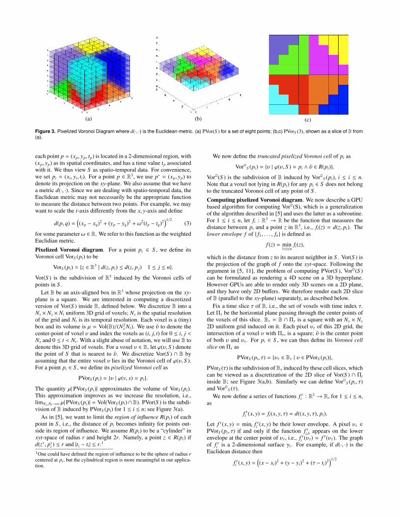
Figure 3. Pixelized Voronoi Diagram where d(·, ·) is the Euclidean metric. (a) PVor(S ) for a set of eight points; (b,c) PVorS (3), shown as a slice of B from(a).

each point p = (xp, yp, tp) is located in a 2-dimensional region, with(xp, yp) as its spatial coordinates, and has a time value tp associatedwith it. We thus view S as spatio-temporal data. For convenience,we set pi = (xi, yi, ti). For a point p ∈ R3, we use p∗ = (xp, yp) todenote its projection on the xy-plane. We also assume that we havea metric d(·, ·). Since we are dealing with spatio-temporal data, theEuclidean metric may not necessarily be the appropriate functionto measure the distance between two points. For example, we maywant to scale the t-axis differently from the x, y-axis and define

d(p, q) =((xp − xq)2 + (yp − yq)2 + ω2(tp − tq)2

)1/2(3)

for some parameterω ∈ R. We refer to this function as the weightedEuclidian metric.

Pixelized Voronoi diagram. For a point pi ∈ S , we define itsVoronoi cell VorS (pi) to be

VorS (pi) = z ∈ R3 | d(z, pi) ≤ d(z, p j) 1 ≤ j ≤ n.

Vor(S ) is the subdivision of R3 induced by the Voronoi cells ofpoints in S .

Let B be an axis-aligned box in R3 whose projection on the xy-plane is a square. We are interested in computing a discretizedversion of Vor(S ) inside B, defined below. We discretize B into aNs × Ns × Nt uniform 3D grid of voxels; Ns is the spatial resolutionof the grid and Nt is its temporal resolution. Each voxel is a (tiny)box and its volume is µ = Vol(B)/(N2

s Nt). We use υ to denote thecenter-point of voxel υ and index the voxels as (i, j, t) for 0 ≤ i, j <Ns and 0 ≤ t < Nt. With a slight abuse of notation, we will use B todenote this 3D grid of voxels. For a voxel υ ∈ B, let ϕ(υ, S ) denotethe point of S that is nearest to υ. We discretize Vor(S ) ∩ B byassuming that the entire voxel υ lies in the Voronoi cell of ϕ(υ, S ).For a point pi ∈ S , we define its pixelized Voronoi cell as

PVorS (pi) = υ | ϕ(v, s) = pi.

The quantity µ|PVorS (pi)| approximates the volume of VorS (pi).This approximation improves as we increase the resolution, i.e.,limNs ,Nt→∞ µ|PVorS (pi)| = Vol(VorS (pi)∩B). PVor(S ) is the subdi-vision of B induced by PVorS (pi) for 1 ≤ i ≤ n; see Figure 3(a).

As in [5], we want to limit the region of influence R(pi) of eachpoint in S , i.e., the distance of pi becomes infinity for points out-side its region of influence. We assume R(pi) to be a “cylinder” inxyt-space of radius r and height 2r. Namely, a point z ∈ R(pi) ifd(z∗, p∗i ) ≤ r and |tz − ti| ≤ r.1

1One could have defined the region of influence to be the sphere of radius rcentered at pi, but the cylindrical region is more meaningful in our applica-tion.

We now define the truncated pixelized Voronoi cell of pi as

VorS (pi) = υ | ϕ(υ, S ) = pi ∧ υ ∈ R(pi).

Vor(S ) is the subdivision of B induced by VorS (pi), i ≤ i ≤ n.Note that a voxel not lying in R(pi) for any pi ∈ S does not belongto the truncated Voronoi cell of any point of S .

Computing pixelized Voronoi diagram. We now describe a GPUbased algorithm for computing Vor(S), which is a generalizationof the algorithm described in [5] and uses the latter as a subroutine.For 1 ≤ i ≤ n, let fi : R3 → R be the function that measures thedistance between pi and a point z in R3, i.e., fi(z) = d(z, pi). Thelower envelope f of f1, . . . , fn is defined as

f (z) = min1≤i≤n

fi(z),

which is the distance from z to its nearest neighbor in S . Vor(S ) isthe projection of the graph of f onto the xyt-space. Following theargument in [5, 11], the problem of computing PVor(S ), Vor(S )can be formulated as rendering a 4D scene on a 3D hyperplane.However GPUs are able to render only 3D scenes on a 2D plane,and they have only 2D buffers. We therefore render each 2D sliceof B (parallel to the xy-plane) separately, as described below.

Fix a time slice τ of B, i.e., the set of voxels with time index τ.Let Πτ be the horizontal plane passing through the center points ofthe voxels of this slice. Bτ = B ∩ Πτ is a square with an Ns × Ns

2D uniform grid induced on it. Each pixel υτ of this 2D grid, theintersection of a voxel υ with Πτ, is a square; υ is the center pointof both υ and υτ. For pi ∈ S , we can thus define its Voronoi cellslice on Πτ as

PVorS (pi, τ) = υτ ∈ Bτ | υ ∈ PVorS (pi),

PVorS (τ) is the subdivision ofBτ induced by these cell slices, whichcan be viewed as a discretization of the 2D slice of Vor(S ) ∩ Πt

inside B; see Figure 3(a,b). Similarly we can define VorS (pi, τ)and VorS (τ).

We now define a series of functions f τi : R2 → R, for 1 ≤ i ≤ n,as

f τi (x, y) = fi(x, y, τ) = d((x, y, τ), pi).

Let f τ(x, y) = mini f τi (x, y) be their lower envelope. A pixel υτ ∈PVorS (pi, τ) if and only if the function f τi,υ appears on the lowerenvelope at the center point of υτ, i.e., f τi (υτ) = f τ(υτ). The graphof f τi is a 2-dimensional surface γi. For example, if d(·, ·) is theEuclidean distance then

f τi (x, y) =((x − xi)2 + (y − yi)2 + (τ − ti)2

)1/2

γi

hi

hi

p∗i

Figure 5. In the case of the Euclidian metric, γi can be simplified usingthe lifting transform.

and its graph is one sheet of a hyperboloid of revolution of twosheets, see Figure 4(a,b). As in [5], PVorS (τ) can be computedby viewing Bτ as the 2D image plane and rendering the surfacesγ1, . . . , γn with (0, 0,−∞) as the viewpoint. We set the color of γi

to i, then the color buffer C[π] stores the index of the point ϕ(π, S ),i.e., the point whose Voronoi cell contains π; see Figure 3(c). Inorder to compute VorS (τ) we need to truncate γi within R(pi), theregion of influence of pi, before rendering it. By repeating this forall slices 0 ≤ t < Nt, we can compute Vor(S ). For a fixed τ, letS τ = p ∈ S | τ − r ≤ tp ≤ τ + r. Then Vor(S , τ) = Vor(S τ, τ).So while computing Vor(S , τ), we only render γi’s for pi ∈ S τ.

Triangulating γi. As mentioned in Section 2, the GPU can ren-der only linear objects. Therefore we need to approximate each γi

(or its truncated version) by a triangulated surface, γi . Here wedescribe the triangulation procedure for the case when d(·, ·) is aconvex function. For technical reasons, we also assume that d(·, ·)does not have a cross term between t and x, y, i.e., we can sep-arate spatial and temporal terms. This implies that d(·, ·) can berestricted to define the distance between two points in R2. We as-sume that γi is such that |ti − τ| ≤ r. Next, we clip γi within pointsπ ∈ R2 s.t. d(π, p∗i ) ≤ r. By our assumption that there are no crossterms, all points on the boundary of the clipped surface γi have thesame z-value. Let γi also denote the resulting surface patch. Next,we choose a parameter m and compute m level-set curves (contourlines) at regular height intervals on γi, i.e., intersect γi with m hor-izontal planes (e.g. dashed circles in Figure 4(c). Each curve isa convex closed curve, which we approximate by a convex k-gon,for some parameter k, by choosing k points on the curve. We thencreate triangles between adjacent k-gons using 2k triangles. Theresulting triangulated surface γi , composed of 2km triangles, ap-proximates γi. See Figure 4(c). the approximation error can becontrolled by choosing the values of m and k carefully.

The case of Euclidean distance. Finally, we show that if d(·, ·) isa weighted Euclidean distance function as defined in (3), there isa much better way of rendering γi using the so-called lifting trans-form [6], which uses fewer triangles and induces no error in thedistance function (though the region of influence is still approxi-mated)

For 1 ≤ i ≤ n, define gτi : R2 → R as

gτi (x, y) = f τi (x, y)2 − x2 − y2

= −2xxi − 2yyi + x2i + y2

i + ω2(ti − τ)2.

Let

gτ(x, y) = mini

gτi (x, y).

The crucial observation is that

gτi (x, y) ≤ gτj(x, y)⇔ f τi (x, y) ≤ f τj (x, y),

which implies that the xy-projection of the lower envelope of fand g are identical, therefore PVors(τ) is also the projection of thegraph of gτ(x, y). We therefore render the graphs of gτi instead of f 2

i .The graph hi of gτi is a 2-dimensional plane, so it can be rendereddirectly. In order to compute Vor(S ), we need to truncate hi withinthe region of influence of hi. We first assume that |ti − τ| ≤ r. Next,let hi be the portion of hi clipped within the region of influence ofpi,

hi = (x, y, z) ∈ hi | (x − xi)2 + (y − yi)2 ≤ r2,

which is an ellipse in 3D. We wish to render h1, . . . , hn. We approx-imate hi to a convex k-gon hi as follows. Let σ be a regular k-gonin R2. We set σi = σ + p∗i . hi is obtained by lifting σi to hi, i.e.,

hi = (x, y, gτi (x, y)) | (x, y) ∈ σi.

For each vertex v of σi there is a vertex (v, gτi ) in hi . We triangu-late hi into k triangles in a standard manner. Note that hi encodesthe function gτi exactly; it only approximates the region of influ-ence.

The GV algorithm. Let GV(S , τ) denote the algorithm, de-scribed in this section, to compute the slice of the truncated pixe-lated Voronoi diagram at time τ, i.e., Vor(S , τ) which is the sameas Vor(S τ, τ). The output of this algorithm is the combination ofcolor bufferC and depth bufferD, which together describe Vor(S , τ).However, we apply the following twist: we set the color of eachtriangle of γi to h(pi) (instead of i). Thus C[π] stores h(pi) forall pixels π ∈ VorS (pi, τ). We define the frame buffer F to be(C,D) and we can think of F as the result of running GV, i.e.,F = GV(S , τ). Ignoring initialization costs, the complexity ofGV(S , τ) is that of rendering γi (or hi ) for each pi within theregion of influence.

4 Natural Neighbor Interpolation on GridsIn this section we describe our algorithms for answering natural-neighbor interpolation queries on a M × M × T grid Q of pointsin R3 using truncated pixelized Voronoi diagrams. We assume thatQ has origin (0, 0, 0) and resolution 1 in each dimension, i.e., Q =0, . . . ,M − 12 × 0, . . . ,T − 1. Any 3D grid can be mapped toQ using an affine transformation and using the weighted Euclidianmetric to preserve the structure of the Voronoi diagram.

Since the region of influence has radius r and height 2r, we de-fine B = Q + [−2r − 1/2, 2r + 1/2]3 — large enough to contain allthe points of S that are of interest, and we can assume that S ⊂ B.For simplicity we assume that r ∈ N. Let s ∈ N be a parameter. Wediscretize B into a sM × sM × T 3D grid of voxels, each voxel isa box of size 1

s ×1s and height 1, and its volume is µ = 1

s2 . By ourdefinition of B and the voxels, each grid point ofQ lies at the centerof an s× s×1 array of voxels of B, i.e., the temporal resolution of Band Q is the same, but the spatial resolution of B is s times that ofQ. One can choose the temporal resolution of B higher than that ofQ but it is not important in our applications and choosing the twoto be the same simplifies the description of the algorithm.

Recall the definition of a the natural neighbor interpolation h :S → R3 given in Equations (1) and (2). In our discretized settingwe modify h as follows:

h(q) =∑

p∈S |VorS (p) ∩ VorS∪q(q)|h(p)|VorS∪q(q)|

=N(q)D(q)

. (4)

P0

P1

P2

(a) (b) (c)

Figure 4. (a,b) Lower envelope of 8 points that were used for PVor(S ) in Figure 3(b,c). (a) shows the hyperboloids from a side view; (b) the outer cellsof the Voronoi diagram are infinite, but in this figure their sizes are limited because the hyperboloids are of a limited height. (c) The triangulation of γiinto γi using two triangle strips (m = 2).

Algorithm # Copies Triangles rendered per p ∈ S# of passes of F General Weighted Euclidean

r2 1 O(r2kmn) O(r2n)r 2r + 1 O(rkmn) O(rn)1 2(2r + 1) O(kmn) O(n)

Table 1. Performance of the three algorithms. |S | = n, each copy of Frequires storing a color buffer and associated depth buffer on the GPU.

D(q) is simply the number of voxels in VorS∪q(q). N(q) is thesum of the heights represented by each voxel in Vor(S ) from theVoronoi cell of q.

We observe that the region of influence along the time axis im-plies that only voxels υ for which |tυ − tq| ≤ r are relevant for N(q)and D(q). Thus, we only need to consider 2r + 1 slices of B corre-sponding to Πtq−r, . . . ,Πtq+r. Applying this to (4) we get

D(q) =tq+r∑τ=tq−r

|VorS∪q(q, τ)| =

tq+r∑τ=tq−r

D(q, τ) (5)

N(q) =tq+r∑τ=tq−r

∑π∈VorS∪q(q,τ)

h(ϕ(π, S )) =

tq+r∑τ=tq−r

N(q, τ), (6)

where

N(q, τ) =∑

π∈VorS∪q(q,τ)

h(ϕ(π, S )),

D(q, τ) = |VorS∪q(q, τ)|.

We refer to Table 1 for an overview of the algorithms presented inthis section.

Let H be an M × M × T array that stores the height at all pointsofQ, computed using the discretized natural-neighbor interpolationdefined in (4). For a fixed time 0 ≤ i < T , let Qi denote the querypoints in time slice i and let Hi denote the corresponding time sliceof H. For a fixed i, by (5) and (6), the computation of Hi involvescomputing Vor(S i−r, i−r), . . . ,Vor(S i+r, i+r). Since we computeeach Hτ separately, a point of S has to be processed by the GPUseveral times. We describe three algorithms that provide tradeoffsbetween the number of times each point of S is processed (whichwe refer to as the number of passes) and the space (on the GPU)used by the algorithm.

r2-pass algorithm.. We process each Qi, for 0 ≤ i < T , sepa-rately. Equations (5) and (6) suggest that we compute N(q, τ) andD(q, τ) for τ = i − r, . . . , i + r and for all q ∈ Qi. For each τ

we first compute Fτ = GV(S , τ), giving us a representation ofVor(S , τ) = Vor(S τ, τ). For q ∈ Qi, let γq denote the graph ofthe function d((x, y, τ), q), which is a 2D surface, and let γq be thelinear approximation of γi, truncated within R(q). Beutel et al [5]have described an algorithm that uses Fτ and renders the surfacesγq | q ∈ Qi so that the color buffer Ci,τ encodes Vor(S ∪q, τ) forall q ∈ Qi. Then using Fτ and Ci,τ it computes N(q, τ) and D(q, τ).We call their algoirthm I(Fτ, i, τ). Depending on the sizeof M, r, s and GPU constraints, this may require several renderingpasses and an I/O-efficient partitioning algorithm; we refer to [5]for details. We assume that the I procedure returns twoM×M arrays N∇ and D∇ s.t. N∇[q] = N(q, τ) and D∇[q] = D(q, τ).The pseudo-code of the algorithm is described in Algorithm 1.

Each point p ∈ S is passed to the computation of O(r) slices ofVor(S τ, τ) for τ ∈ btpc−r, . . . , dtpe+r. Furthermore each Voronoidiagram slice Vor(S , τ) is computed 2r+1 times forQτ−r, . . . ,Qτ+r.Hence each point of S is passed O(r2) times.

Algorithm 1 r2-passfor i← 0 to T − 1 do

Hi ← Ni ← Di ← 0for τ ∈ i − r, . . . i + r doF← GV(S τ, τ)(N∇,D∇) = I(F, i, τ)Ni ← Ni + N∇, Di ← Di + D∇

Hi ← Ni/Di

return H

r-pass algorithm. The overall structure of the algorithm is thesame as before but we save some computation by storing what wehave already computed and re-using it. As before, let frame bufferFτ = GV(S , τ) refer to the combination of Cτ and Dτ describingVor(S , τ). To answer NNI queries for points in Qi we must gen-erate Fi−r, . . .Fi+r and perform the interpolation on each time-slice.When we proceed to Qi+1, we must now generate Fi+1−r, . . .Fi+1+r.We have all of the frame buffers except the last, Fi+1+r, from the pre-vious step and thus they can be reused by I step. We onlyneed to call GV(S i+1+r, i+1+r). See Algorithm 2 for the pseudo-code. This algorithm requires storing 2r + 1 frame buffers: 2r tosave values from the previous query grid and one to generate thenew Voronoi diagram. Doing this for Qi for all 0 ≤ i < M in orderlets us generate each Fi only once. This method renders each pointp O(r) times: once for each Vor(S τ, τ) for τ ∈ btpc−r, . . . , dtpe+r.1-pass algorithm. We now show that the number of passes canbe reduced to 1 if S is time series data and d(·, ·) satisfies certain

Algorithm 2 r-passCreate F−r−1 . . . Fr−1

for i← 0 to T − 1 doHi ← Ni ← Di ← 0Delete Fi−r−1 from GPUFi+r ← GV(S i+r, i + r)for τ ∈ i − r, . . . i + r do

(N∇,D∇) = I(Fτ, i, τ)Ni ← Ni + N∇, Di ← Di + D∇

Hi ← Ni/Di

return H

properties and the GPU supports certain primitives. For simplicity,we assume that S = Σ1 ∪ Σ2 ∪ · · · , where the t-coordinate of allpoints in Σi is i, the time coordinate of the ith slice ofQ, and d(·, ·) isthe weighted Euclidian distance. The first assumption can easily beremoved. The second assumption can be relaxed to a larger familyof distance functions, but identifying this family is technical andomitted from this version. Recall that Vor(Σi, j) is the projection ofthe lower envelope gi

j(x, y) of the functions

gij,p(x, y) = −2xxp − 2yyp + x2

p + y2p + ω

2( j − i)2 ∀p ∈ Σi (7)

Since the last term in (7) does not depend on p, it immediatelyimplies that Vor(Σi, j) is the same for all j and that

gij(x, y) = gi

i(x, y) + ω2( j − i)2.

Let Fij = (Ci

j,Dij) = GV(Σi, j) — Ci

j[π] stores the height of thepoint nearest to π and Di

j stores the distance from π to its nearestneighbor, and let Fi = Fi

i. Then Fij can be computed from Fi by

adding the value ω2( j − i)2 to every pixel in Di. Let S(F, δ) bethe procedure that adds the value δ to all pixels in D. Then

Fij = S(Fi, ω2( j − i)2).

Recall that S j =⋃r`=−r Σ

j+`. Assuming we have F` for j − r ≤ ` ≤j + r, we can compute the frame buffer F j = (C j,D j) correspond-ing to Vor(S j, j), using the procedure C(F j−r, . . . ,F j+r) asfollows. We first compute F`j for j − r ≤ ` ≤ j + r, and set

D j[π] = minj−r≤`≤ j+r

D`j[π]

and finally set C j[π] to the contents of C`j[π] if D j[π] = D`j[π]. Thepseudo-code can be found in Algorithm 3.

Algorithm 3 C(F j−r, . . . ,F j+r)for all π ∈ F j doC j[π]← 0, D j[π]← ∞

for i ∈ j − r, . . . , j + r doFi

j ← S(Fi, ω2( j − i)2)for all π ∈ F j do

if Dij[π] < Di[π] thenD j[π]← Di

j[π]C j[π]← Ci

j[π]return F j

With these procedures at hand, we modify the r-pass algorithmas follows, so that each point is processed once. See Algorithm 4for the pseudo-code. The algorithm maintains the invariant thatwhile processingQi, it maintains Fi−r, . . . ,Fi+r and also Fi, . . . ,Fi+2r.While processing of Qi, the algorithm first computes Fi+2r usingGV(Σi+2r, i + 2r). Next, instead of computing Fi+r by invoking

Σi Σi+1

Fi Fi+1

Fii−∆ . . . Fi

i, Fii+1 . . . Fi

i+∆ Fi+1i+1−∆ . . . Fi+1

i , Fi+1i+1 . . . Fi+1

i+1+∆

Fi Fi+1

Combine Combine

. . .. . .

GVor

Shift

Figure 6. The process of creating Fi from sets of data Σi rendering eachpoint only once.

GV(S i+r, i+r), it uses the procedure C(Fi, . . . ,Fi+2r). Therest of the procedure is the same. Note that each point is processedonly once.

Algorithm 4 1-pass

Create F−1 . . .F2r−1 and F−r−1 . . . Fr−1

for i← 0 to T − 1 doH(Qi)← N(Qi)← D(Qi)← 0Delete Fi−1 and Fi−r−1 from GPUFi+2r ← GV(Σi+2r, i + 2r)Fi+r ← C(Fi . . .Fi+2r)for τ ∈ i − r, . . . i + r do

(N∇,D∇) = I(Fτ, i, τ)Ni ← Ni + N∇, Di ← Di + D∇

Hi ← Ni/Di

return H

5 Experimental ResultsWe now discuss the details of the implementation and testing ofTerraNNI. It is implemented in C++ and use OpenGL for renderingon the GPU. We ran our experiments on an Intel Core2 Duo CPUE6850 at 3.00GHz with 8GB of internal memory. We used Ubuntu10.4 and two 1TB SATA disk drives in a RAID0 configuration.Additionally, the machine contained a NVIDIA GeForce GTX 470graphics card running CUDA 3.0. This card has 1.2GB of memory,448 CUDA cores, and 14 multiprocessors.

Data sets. We ran TerraNNI on two data sets. We performed amajority of our tests on LiDAR data collected from the Nags Head,NC region for years 1997-1999, 2001, 2004, 2005, 2007, and 2008.The data ranges from 100,000 points per year to nearly 3 millionpoints per year and comes to a total of just under 20 million points.This data set takes up 382 megabytes on disk. We will refer to thisdata set as the NC coastal data set. The data is freely available at[1] and was provided to us by Helena Mitasova.

We also performed tests on a much larger LiDAR data set col-lected from Fort Leonard Wood in Missouri (data courtesy of theU.S. Army Corps of Engineers) in 2009 and 2010. The data setconsists of approximately 450 million data points over an 80.5km2

region and takes up 8.8GB on disk.

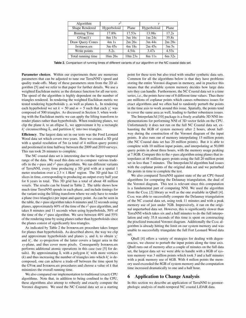
Algorithm r2 rShape Rendered Hyperboloid Plane Hyperboloid PlaneBinning Time 17.89s 17.53s 13.98s 17.2s

GV(S ) 8m 15s 3m 16s 1m 24s 35.8sDraw Query Cones 4m 1s 2m 26s 3m 44s 2m 28s

I 3m 45s 4m 18s 2m 45s 3m 5sWrite points 5.2s 4.54s 3.47s 4.53s

Total running time 16m 26s 10m 23s 8m 11s 6m 32s

Table 2. Comparison of running times of different variants of our algorithm on the NC coastal data set.

Parameter choices. Within our experiments there are numerousparameters that can be adjusted to tune our TerraNNI’s speed andquality trade-offs. Many of these parameters stem from the 2D al-gorithm [5] and we refer to that paper for further details. We use aweighted Euclidean metric as the distance function for all our tests.The speed of the algorithm is highly dependent on the number oftriangles rendered. In rendering the weighted Euclidean metric wetested rendering hyperboloids γi as well as planes hi. In renderingeach hyperboloid we set k = 50 and m = 5 such that each γi wascomposed of 500 triangles. As discussed in Section 3, when work-ing with the Euclidean metric we can apply the lifting transform torender planes rather than hyperboloids. When rendering planes, weclip the plane hi to an ellipse hi, we approximate it by a rectanglehi circumscribing hi, and partition hi into two triangles.Efficiency. The largest data set in our tests was the Ford LeonardWood data set which covers two years. Here we created a 3D gridwith a spatial resolution of 5m (a total of 4 million query points)and positioned in time halfway between the 2009 and 2010 surveys.This run took 26 minutes to complete.

The NC coastal data set is interesting due to the larger temporalrange of the data. We used this data set to compare various trade-offs in the r-pass and r2-pass algorithms. We ran different variantsof TerraNNI, every time producing a 3D grid with at a spatial 1meter resolution over a 2.3 × 1.8km2 region. The 3D grid has 12slices in time, corresponding to producing an output every half yearfor 6 years in total. This 3D grid has a total of about 48 millionvoxels. The results can be found in Table 2. The table shows howmuch time TerraNNI spends in each phase, and include timings forthe variant using the lifting transform where we only have to rendera plane (two triangles) per input and query point. As can be seen inthe table, the r-pass algorithm takes 6 minutes and 32 seconds usingplanes, approximately 60% of the time of the r2-pass algorithm, andtakes 8 minutes and 11 seconds when using hyperboloids, 50% ofthe time of the r2-pass algorithm. We save between 40% and 55%of the rendering time by using planes rather than hyperboloids sincethe planes consist of significantly less triangles.

As indicated by Table 2 the I procedure takes longerfor planes than hyperboloids. As described above, the way we clipand approximate hyperboloids and planes γi and hi to obtain γiand hi , the xy-projection of the latter covers a larger area in thexy-plane, and thus cover more pixels. Consequently Iperforms additional atomic operations in this case (see [5] for de-tails). By approximating hi with a polygon hi with more vertices(k) and thus increasing the number of triangles into which hi is de-composed, one can achieve a trade-off between the time spent bythe GV and I procedures and choose a value of k thatminimizes the overall running time.

We also compared our implementation to traditional (exact) CPUalgorithms. Note that, in addition to being confined to the CPU,these algorithms also attemp to robustly and exactly compute theVoronoi diagrams. We used the NC Coastal data set as a starting

point for these tests but also tried with smaller synthetic data sets.Common for all the algorithms below is that they have problemsstoring the entire Voronoi diagram in memory, and in practice thismeans that the available system memory decides how large datasets they can handle. Furthormore, the NC Coastal data set is a timeseries, i.e., the points have one of 8 different time values. Thus thereare millions of coplanar points which causes robustness issues forexact algorithms and we often had to randomly perturb the pointsin the time axis to work around this issue. Spatially, the points tendto cover the same area as well, leading to further robustness issues.

The Interpolate3d [10] package is a freely available 3D NNI im-plementations for performing NNI of 3D vector fields on the CPU.Unfortunately it does not run on the full NC Coastal data set, ex-hausting the 8GB of system memory after 2 hours, about half-way during the construction of the Voronoi diagram of the inputpoints. It also runs out of memory interpolating 15 million points(the NC Coastal data set has 20 million points). But it is able tocomplete with 10 million input points, and interpolating at 50,000query points in about three hours, with the memory usage peakingat 7.8GB. Compare this to the r-pass algorithm using planes that in-terpolates at 48 million query points using the full 20 million pointset in less than 7 minutes. The Interpolate3d algorithm had issueswith the coplanar points of the original data set and we perturbedthe points in time to complete the test.

We also compared TerraNNI against state of the art CPU-basedalgorithms for computing the Delaunay triangulation, the dual ofthe Voronoi diagram. This test is relevant since this computationis a fundamental part of computing NNI. We used the algorithmfrom the C [2] library as well as the one available in Qhull [4].C was able to successfully compute the Delaunay triangulationof the NC coastal data set, using took 11 minutes and with a peakmemory use of just under 7GB. Impressively, it ran on the origi-nal unperturbed data set. However, this is significantly slower thanTerraNNI which takes six and a half minutes to do the full interpo-lation and only 35.8 seconds of this time is spent on constructingthe pixelized truncated Voronoi diagram. Additionally the C al-gorithm is already hitting the limit on our system memory and wasunable to successfully triangulate the full Fort Leonard Wood dataset.

Qhull [4] offers a variety of strategies for dealing with degen-eracies, we choose to perturb the input points along the time axis.Qhull runs out of memory after a couple of minutes on the full dataset, the largest data set we were able to handle with a 8GB of sys-tem memory was 3 million points which took 3 and a half minuteswith a peak memory use of 6GB. With 4 milion points the mem-ory used exceeded the 8GB of system memory and the computationtime increased dramatically to one and a half hour.

6 Application to Change AnalysisIn this section we describe an application of TerraNNI to geomor-phologic analysis of multi-temporal NC coastal LiDAR data.

(a) Regression slope values for cmin = 0 (b) Regression slope values for cmin = 0.85

Figure 7. Regression line slope values from year 2000 to 2006 superimposed on year 2000 DEM.

Figure 1(c) gives a map of Nags Head, NC. The focus of our ap-plication study is Jockey’s Ridge state park sand dune. Specifically,we investigate the annual sand dune growth and erosion from years2000 to 2006. In order to perform the study, first we apply Ter-raNNI to interpolate a digital elevation model (DEM) for each yearfrom 2000 to 2006, inclusively, since many of the yearly collects(e.g., 2000, 2002, and 2003) are not available. We set the radiusof influence to 2. Second, we estimate a linear regression modelfor each pixel and all of its temporal neighbors (i.e., years 2000 to2006). For example, if p(x, y, t) is the pixel value (height) at lo-cation (x, y) and time t, a linear regression model is estimated forthe set p(x, y, t1), . . . , p(x, y, tn). Third, we apply the change anal-ysis method of [16] by examining the rates of change (i.e., slopes)of the model estimates for pixel observations that exhibit stronglinear trends. As in [16], we define the notion of a coefficient ofdetermination χ: a measure of the reliability of the linear modelin predicting the pixel values (response variable), χ ∈ [0, 1] is ex-pressed as follows: χ = 1 − (SSerr/SStot) where SSerr is the sum ofsquared errors between the linear model’s estimates and responsevariable and SStot is the total sum of squared deviations of the re-sponse variable to its expectation [7]. A high χ implies that theSSerr is relatively small compared to SStot, indicating that the linearmodel can well predict the sample observations. We set a thresholdvalue cmin and choose those pixels for which χ ≥ cmin. The thresh-old cmin can be regarded as the minimum proportion of the variationin the response variable that is captured by the linear model.

Figure 7(a) depicts the slope values for the entire sand dune re-gion for cmin = 0. Strong erosions (negative slopes) are observed inthe northwest region with extensive accumulation (positive slopes)in the southeast area of the dune. This erosion and accumulationsuggest a net wind force pattern movement towards the southeastdirection; however, these observed slope values do not convey ad-ditional information on the nature of the movements throughoutthe years. But by using the linear regression estimates, further in-sights into the inter-annual patterns can be harnessed by extractingthose composite movements that exhibit a linear trend. We can de-termine these linearly dependent patterns by pruning those DEMpixels that have large deviations from the regression model, whichis achieved by increasing cmin. Figure 7(b) shows the slope valuesfor cmin = 0.85. In this figure, we can see regions of the dune whichhave undergone continuous changes following a predominantly lin-ear trend. We exemplify these changes for year 2002 to 2004 inFigure 8. From 2002 to 2003, the measured total sand growth and

erosion are 20512 m3 and 82714 m3, respectively. For years 2003to 2004, similar level of dune activity is observed with total growthand erosion volumes of 33895 m3 and 74809 m3, respectively. Be-cause the proposed NNI approach can efficiently interpolate themissing DEMs in both space and time, geomorphologic analysessuch as the one demonstrated in this case study can be rapidly andeffectively executed on large areas and at high resolutions.

7 ConclusionIn this paper we have presented three algorithms for performing(discretized) NNI on a 3D grid using a GPU. The three algorithmsprovide different tradeoffs between GPU computational complexityand GPU memory requirement ranging from storing one buffer onthe GPU and processing each input point a quadratic (in r) numberof times, to processing each input point one time, but with memoryuse linear in the time region of influence. Furthermore, we usedthe lifting transform to limit the polygonal complexity of the sur-faces used for each point, shifting the bottleneck away from ren-dering triangles. Our algorithm, and its implementation, scale tovery large data sets and the underlying discretization works aroundthe robustness problems that add additional complexity to existingCPU-based algorithms. We are unaware of any robust implementa-tion of NNI for points in R3 that can handle large data sets.

Our experimental results gives an example of an application ofour algorithm and suggests that is practical in real world situations,outperforming exact CPU algorithms on medium sized data setsand enabling the efficient processing on even larger data sets withlimited memory requirements. We plan on making our implemen-tation of TerraNNI publicly available.

AcknowlegdementsThe authors thank Helena Mitasova and the U.S. Army Corps ofEngineers for access to data and and Tamal Dey and Danny Halperinfor helpful discussions.

References[1] NOAA coastal services center, LI-

DAR data retrieval tool. http://csc-s-maps-q.csc.noaa.gov/dataviewer/viewer.html?keyword=lidar.

[2] C, Computational Geometry Algorithms Library.http://www.cgal.org.

(a) Changes from 2002 to 2003 superimposed on 2002 DEM (b) Changes from 2003 to 2004 superimposed on 2003 DEM

Figure 8. Yearly changes (meters) for areas with regression model coefficient of determination ≥ 0.85.

[3] D. Attali and J.-D. Boissonnat. A linear bound on the com-plexity of the Delaunay triangulation of points on polyhedralsurfaces. Discrete & Computational Geometry, 31:369–384,2004.

[4] C. B. Barber, D. P. Dobkin, and H. Huhdanpaa. The quick-hull algorithm for convex hulls. ACM Trans. on MathematicalSoftware, 22(4):469–483, 1996.

[5] A. Beutel, T. Mølhave, and P. K. Agarwal. Natural neighborinterpolation based grid DEM construction using a GPU. InProc. 18th ACM SIGSPATIAL International Symposium onAdvances in Geographic Information Systems, pages 172–181, 11 2010.

[6] M. de Berg, M. van Kreveld, M. Overmars, andO. Schwarzkopf. Computational Geometry – Algorithms andApplications. Springer Verlag, 1997.

[7] N. Draper and H. Smith. Applied Regression Analysis. Wiley-Interscience, 3rd edition, 1998.

[8] Q. Fan, A. Efrat, V. Koltun, S. Krishnan, and S. Venkatasub-ramanian. Hardware-assisted natural neighbor interpolation.In Proc. 7th Workshop on Algorithm Engineering and Exper-iments (ALENEX, 2005.

[9] S. Ghosh, A. E. Gelfand, and T. Mølhave. Attaching un-certainty to deterministic spatial interpolations. StatisticalMethodology, 2011. In Print.

[10] R. Hemsley. Interpolation on a magnetic field. 2009.http://code.google.com/p/interpolate3d/.

[11] K. E. Hoff, III, J. Keyser, M. Lin, D. Manocha, and T. Cul-ver. Fast computation of generalized Voronoi diagrams usinggraphics hardware. In Proc. 26th Annual Conference on Com-puter Graphics and Interactive Techniques, pages 277–286,1999.

[12] P. C. Kyriakidis and A. G. Journel. Geostatistics space-timemodels: A review. Mathematical Geology, 31(6):651–684,1999.

[13] L. Li and P. Revesz. A comparison of spatio-temporal interpo-lation methods. In Geographic Information Science, volume2478, pages 145–160. Springer, 2002.

[14] J. Mateu, F. Montes, and M. Fuentes. Recent advances inspace-time statistics with applications to environmental data:An overview. Geophysical Research, 108(8774), 2003.

[15] E. Miller. Towards a 4D-GIS: four dimensional interpolationutilizing kriging. In Z. Kemp, editor, Innovations in GIS 4,pages 181–197. 1997.

[16] H. Mitasova, E. Hardin, M. Overton, and R. Harmon. Newspatial measures of terrain dynamics derived from time se-ries of lidar data. In Proc. 17th International Conference onGeoinformatics, pages 1–6, 2009.

[17] H. Mitasova, L. Mitas, W. M. Brown, D. P. Gerdes, I. Kosi-novsky, and T. Baker. Modeling spatially and temporally dis-tributed phenomena: new methods and tools for GRASS GIS.International Journal of Geographical Information Systems,9(4):433–446, 1995.

[18] H. Mitasova, M. Overton, and R. S. Harmon. Geospatial anal-ysis of a coastal sand dune field evolution: Jockey’s ridge,north carolina. Geomorphology, 72(1-4):204 – 221, 2005.

[19] T. Mølhave, P. K. Agarwal, L. Arge, and M. Revsbæk. Scal-able algorithms for large high-resolution terrain data. In Proc.1st International Conference and Exhibition on Computingfor Geospatial Research & Application. ACM, 2010.

[20] NVIDIA. CUDA homepage. http://nvidia.com/cuda, 2010.3.0.

[21] J. D. Owens, D. Luebke, N. Govindaraju, M. Harris,J. Krüger, A. Lefohn, and T. J. Purcell. A survey ofgeneral-purpose computation on graphics hardware. Com-puter Graphics Forum, 26(1):80–113, 2007.

[22] S. Shekhar and H. Xiong, editors. Encyclopedia of GIS.Springer, 2008.

[23] R. Sibson. A brief description of natural neighbour interpo-lation. In V. Barnet, editor, Interpreting Multivariate Data,pages 21–36. John Wiley & Sons, Chichester, 1981.

[24] C. K. Wikle, L. M. Berliner, and N. Cressie. HierarchicalBayesian space-time models. Environmental and EcologicalStatistics, 5:117–154, 1998.