Laura Hurd

Terrain Processing of Sanderson, Texas Dr. Maidment, Marcelo Somos, Rachel Chisolm, Cody Hudson and I worked on producing a new flood plain map for Sanderson, Texas. We worked with Glenn Wright (AECOM), Melinda Luna (TWDB), the city of Sanderson and Trent Lott (NRCS).

Sanderson is a small border town 5.5 hours west of Austin and the county seat for Terrell County. The area had a very devastating flood back in the 1960s which killed 28 people in the town. This spurred the Natural Resources Conservation Service (NRCS) to do their own study of the area to prevent something like this from happening again. NRCS decided to build 11 dams upstream of Sanderson and completed the last of 11 dams in 1987. The town has a pre-dam flood plain map which is obsolete. Our job is to update the flood plain map by taking the dams into consideration and hopefully reduce the flood insurance rates for the people of Sanderson.

The three key elements to look at when producing a flood map are the hydrology, hydraulics of the dams and the terrain processing of the area. I will be focusing on the terrain processing. For now I will work with the topographically derived NED data available.

The Data: • NED data was in 1/3 arcsecond (~10m) grid and taken off the seamless website

(http://seamless.usgs.gov/). • 100k NHD flowline, HUC-8 watershed, HUC-12 watershed data from the USGS website

(http://nhd.usgs.gov/data.html). • To find out where Sanderson was I downloaded TIGER census data such as countylines,

census blocks and roads for Terrell County (http://www2.census.gov/cgi-bin/shapefiles2009/county-files?county=48443).

• GCS coordinates for the 11 dams were provided by Darrel Siedel. • Elevation datum NAVD88 Benchmarks from the NOAA website for the Sanderson

watershed • Auxillary Spillway elevations were from Cody Hudson (he got them from Trent Lott) • 1977 DFIRM from the FEMA website

The Pre-Processing: First, I took the NED data and projected it using UTM Zone 13 and made each cell 10X10m. Then I found the HUC8 watershed that Sanderson was in and dissolved, projected and converted it to a raster with each cell having a value of 1 and being 10X10m. Then I multiplied the projected NED data with the HUC8 I dissolved. This got me the DEM of the watershed Sanderson was in (HUC 8-13040208).

Then I took this new DEM and reconditioned it by burning the NHD Flowlines into the terrain. This produced the AGREEDEM. The AGREEDEM alters the DEM to make the water go into the streams. Then I filled in the sinks and ran the dendritic terrain processing tool. The output of the tool was the flow accumulation, catchments, drainage points, drainage lines etc. for the terrain.

The terrain processing is used to make relatively accurate stream and river cross-sections which will then be used in the hydraulics processing to look at different flooding situations. The flow accumulation and catchments are also needed for Hydrology processing.

Accuracy:

The accuracy of the DEM needed to be assessed. I did this by comparing the vertical elevations from the geodetic benchmarks with high levels of stability (A and B) to the elevation from the DEM. Using the info tool in GIS I clicked on each benchmark and got the DEM elevation for that point and the Benchmark elevation for that point. After I did this for all 66 of the benchmarks I compared the elevations. It was found that the average accuracy (benchmark elevation minus DEM elevation)was -1.44 feet. The standard deviation was found to be 12.16 feet which means there is high variability in the accuracy. The accuracy prescribed by FEMA is 2.4 feet for hilly or rolling terrain (4 foot contour intervals) and the average accuracy for NED data is 14.9ft. Our NED data fits on average the FEMA standard, but there is very high variability with our average. This means we need more accurate elevation data.

I also looked at Ortho-imagery quads and used them to compare the terrain with the DEM. I found 1:12,000 digital, mosaic 7.5 minute quads at the datagateway website (http://datagateway.nrcs.usda.gov/).

Figure 1: Ortho-imagery quads

Study Area:

a)

 b)  

Figure 2: a) The elevation is in feet and the study area spans across Brewster, Pecos and Terrell County. There are 11 dam sites all labeled according to the document from Darrel Siedel.. b) the blue arrow points to the lagoons

It was realized during the trip to Sanderson that our study area would be to the Lagoons which were about 3 miles south east of Sanderson off of Highway 90. In light of this I produced a DEM of the Sanderson watershed that only went down to the lagoons as seen in figure 2 so that the elevation difference in the watershed could be seen. I did this by boxing the area with a graphic polygon and converting that graphic into a feature and then converting the feature into a raster and then reclassifying the raster to have the value of 1. Then I multiplied the reclassified

raster by the HUC8 DEM produced above to get the watershed raster to the lagoons. The study area has a pretty steep slope illustrated by the 2500ft drop over 30 miles which gives a 1.7% slope. This terrain is classified as “hilly” with its sharp terrain and steep canyons.

One can also see in figure 2a that all the dam sites are marked and labeled. I took the dam locations from Darrel Siedel and input them into GIS by importing the excel spreadsheet and creating point features with the dams’ longitude and latitude. Then I projected the dam sites using UTM zone 13.

Dam Capacity:

The dams play a very large roll in this study and they are the reason we are doing this study. I thought it would be appropriate to look at the area that would be covered with water behind the dam if the water reached the emergency (auxillary) spillway. To do this I took the auxillary spillway elevation and found that elevation from the DEM next to the site of interest and created a contour for the elevation. Then I made a polygon graphic following the contour to find the auxillary water coverage. I then converted the graphic into a feature.

Figure3: auxillary dam capacity feature for site 3. The arrow is pointing to the spillway

Figure4:  dam capacity features for all 11 dam sites 

Flooding: 

Rachel produced inundation maps using Geo‐HecRAS for the 1965 flood, and the 100 year flood with and without dams. I wanted to compare the different floods to one another so I compared each 100 year flood scenario with the 1965 flood.  The results can be seen in figure 5 

 

Figure 5:  Inundation maps 

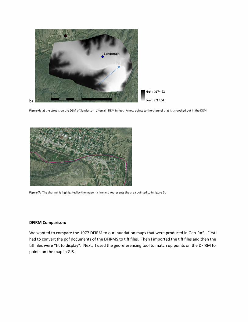
The issue with the inundation maps that Rachel produced were that they didn’t accurately represent the flood especially on the east bend.  This is due to the inaccuracy from the DEM.  The DEM is smooth in the east bend and doesn’t accurately show the channel that we saw when we went to Sanderson.  This can be seen in figure 6. 

a)  

b)  

Figure 6:  a) the streets on the DEM of Sanderson  b)terrain DEM in feet.  Arrow points to the channel that is smoothed out in the DEM 

  

 

Figure 7:  The channel is highlighted by the magenta line and represents the area pointed to in figure 6b 

 

 

DFIRM Comparison: 

We wanted to compare the 1977 DFIRM to our inundation maps that were produced in Geo‐RAS.  First I had to convert the pdf documents of the DFIRMS to tiff files.  Then I imported the tiff files and then the tiff files were “fit to display”.  Next,  I used the georeferencing tool to match up points on the DFIRM to points on the map in GIS. 

 

Figure 8:  1965 inundation compared with original DFIRM 

Conclusion:

The conclusion that we took away from this study was that we need more accurate terrain data. The comparison from the benchmarks and DEM showed this with the high variability of accuracy. We also saw from the zoom in of Sanderson terrain in Figure 6 that the DEM does not accurately represent the channel. This is an important piece to the inundation maps. We are hoping to get higher resolution LIDAR maps for this terrain so that we could do a more thorough study.