The Sanderson Project - University of Texas at Austin · The Sanderson Project ... has to rely on a...
22
UNIVERSIY OF TEXAS The Sanderson Project Using SITES to determine the S v.s Q Relationship By: Cody B. Hudson 5/7/2010
Transcript of The Sanderson Project - University of Texas at Austin · The Sanderson Project ... has to rely on a...

UNIVERSIY OF TEXAS
The Sanderson Project
Using SITES to determine the S v.s Q Relationship
By: Cody B. Hudson
5/7/2010
Table of Contents
Introduction .................................................................................................................................... 1
Data Gathering ................................................................................................................................ 3
SITES Background ............................................................................................................................ 3
Watershed Schematic ..................................................................................................................... 4
Hydrology ........................................................................................................................................ 5
Hydraulics ........................................................................................................................................ 9
River Routing ................................................................................................................................. 18
Model Results ............................................................................................................................... 19
Conclusions ................................................................................................................................... 20
Works Cited ................................................................................................................................... 20
1
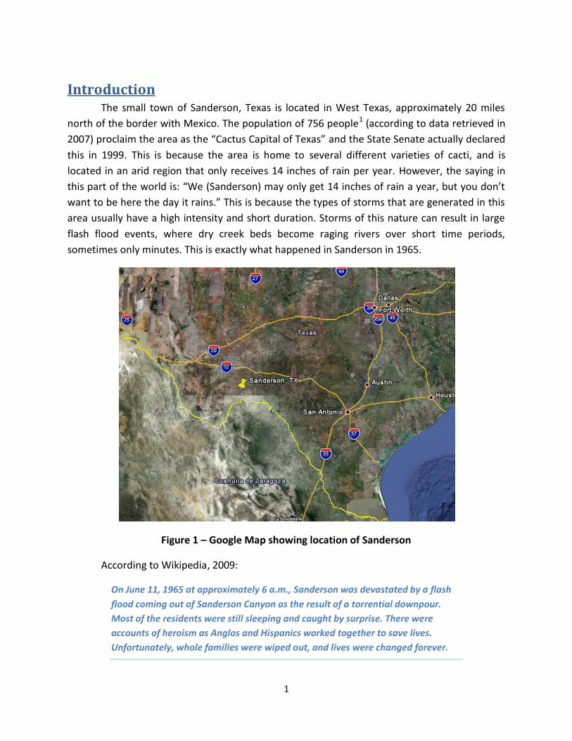
Introduction The small town of Sanderson, Texas is located in West Texas, approximately 20 miles
north of the border with Mexico. The population of 756 people1 (according to data retrieved in
2007) proclaim the area as the “Cactus Capital of Texas” and the State Senate actually declared
this in 1999. This is because the area is home to several different varieties of cacti, and is
located in an arid region that only receives 14 inches of rain per year. However, the saying in
this part of the world is: “We (Sanderson) may only get 14 inches of rain a year, but you don’t
want to be here the day it rains.” This is because the types of storms that are generated in this
area usually have a high intensity and short duration. Storms of this nature can result in large
flash flood events, where dry creek beds become raging rivers over short time periods,
sometimes only minutes. This is exactly what happened in Sanderson in 1965.
Figure 1 – Google Map showing location of Sanderson
According to Wikipedia, 2009:
On June 11, 1965 at approximately 6 a.m., Sanderson was devastated by a flash
flood coming out of Sanderson Canyon as the result of a torrential downpour.
Most of the residents were still sleeping and caught by surprise. There were
accounts of heroism as Anglos and Hispanics worked together to save lives.
Unfortunately, whole families were wiped out, and lives were changed forever.

2
During a recent visit to Sanderson it became evident that lives were indeed changed forever. At
the county courthouse several residents that were in Sanderson during the flood came to speak
to our group. As they recounted the events of the flood you could almost feel what it was like
to be there. Also, in the courthouse a simple plaque displays the names of the people lost in the
flood (Figure 2).
Figure 2 – Sanderson Flood Victims Plaque
As a result of this flood, eleven flood control dams were constructed by the Natural
Resources Conservation Service (NRCS) on the rivers upstream of the town, but no floodplain
analysis has been conducted since the dams were completed in the 1980’s. The town currently
has to rely on a Flood Insurance Rate Map (FIRM) that was last revised in 1977. This has
resulted in many townspeople having to pay for costly flood insurance that may not be
necessary due to the flood control structures. The problem is that small towns such as
Sanderson may not have the resources they need in order to get a FIRM revision. To help
3
alleviate some of the cost of the study and inform the citizens of Sanderson about the
floodplain study process, a group of students at the University of Texas, with the help of
AECOM and the NRCS, have taken on the task of beginning a floodplain analysis for the town.
The main task that this paper will focus on is the use of the NRCS SITES program to determine
the relationship between outflow (Q) and Storage (S) at the eleven dam sites. Also, a hydrologic
model, which was constructed for the entire basin will be discussed.
Data Gathering Before any work could be done in the SITES program, several pieces of information
needed to be gathered, including: construction plans, basin characteristics, and a design
rainfall. During the visit to Sanderson a very fortuitous stop at a gas station resulted in meeting
the State Design Engineer for the USDA-NRCS, Trent Street. Trent was exactly the person that
this project needed in order to get the information for this study. All the information was
gathered from files at the USDA by Trent and his staff and delivered to our group at a meeting
in Trent’s office in Temple, TX.
The construction plans for all eleven dams were given in an electronic form. The
information in these plans was the key to determining the hydraulic routing through the dams.
In particular, the elevation-storage relationship, principal spillway characteristics, and auxiliary
spillway characteristics were needed in order to calculate the outflow from each dam.
The basin characteristics and design rainfall were also given by an analysis that the NRCS
has done before the construction of the dams. The information in these reports served as the
basis for the hydrological analysis. These reports would be outdated in many basins if extensive
development had occurred, but in this region there has been virtually no change. Therefore, the
use of these parameters is believed to be sufficient.
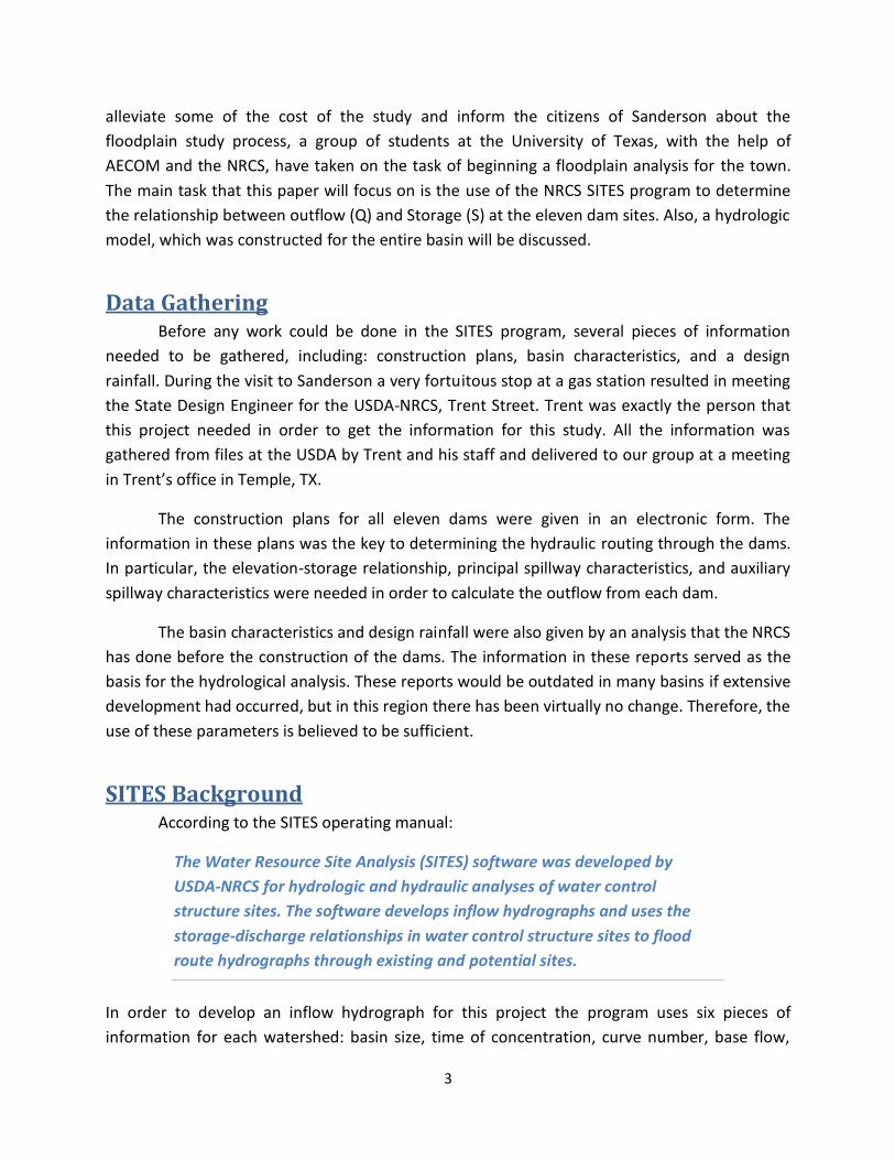
SITES Background According to the SITES operating manual:
The Water Resource Site Analysis (SITES) software was developed by
USDA-NRCS for hydrologic and hydraulic analyses of water control
structure sites. The software develops inflow hydrographs and uses the
storage-discharge relationships in water control structure sites to flood
route hydrographs through existing and potential sites.
In order to develop an inflow hydrograph for this project the program uses six pieces of
information for each watershed: basin size, time of concentration, curve number, base flow,
4
rainfall distribution and rainfall amount. This information allows the program to develop a
hydrograph based on the rainfall for the watershed that takes into account initial abstractions
and base flow. The next step is then to take the inflow (I), with the storage (S) characteristics of
the dam and determine the outflow (Q). To do this a hydraulic analysis on the dam’s spillways
must be conducted. The following sections will discuss how this was accomplished using the
SITES program.
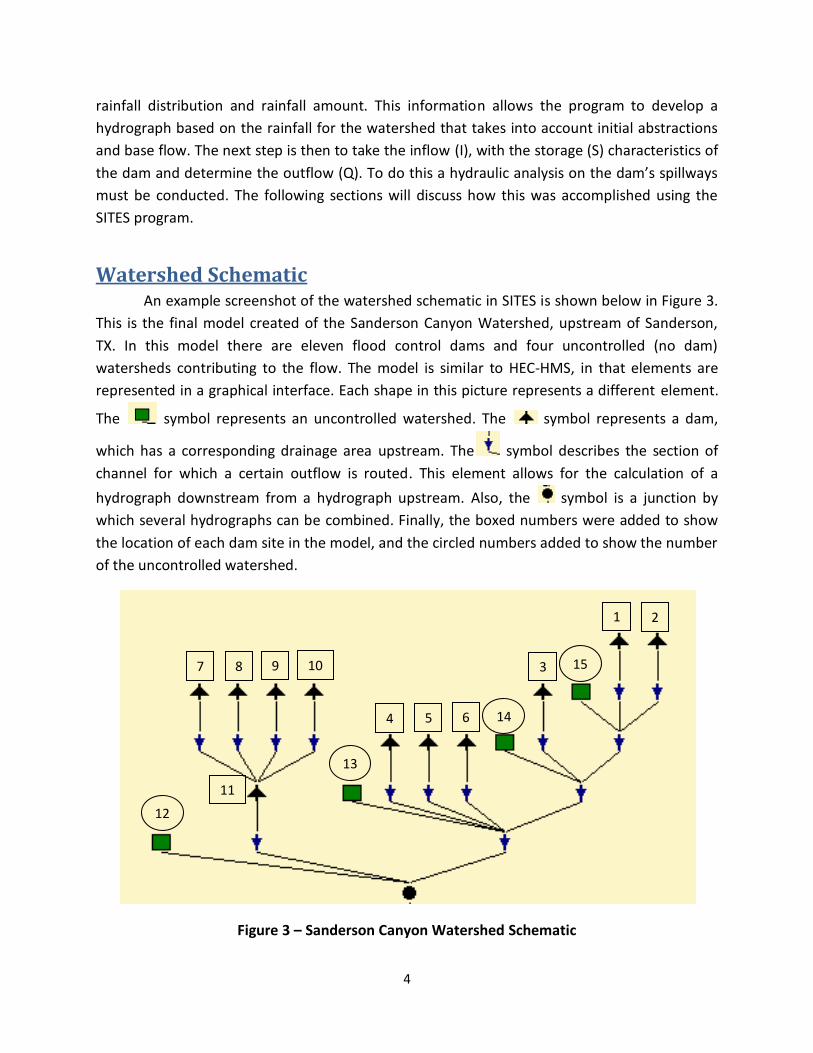
Watershed Schematic An example screenshot of the watershed schematic in SITES is shown below in Figure 3.
This is the final model created of the Sanderson Canyon Watershed, upstream of Sanderson,
TX. In this model there are eleven flood control dams and four uncontrolled (no dam)
watersheds contributing to the flow. The model is similar to HEC-HMS, in that elements are
represented in a graphical interface. Each shape in this picture represents a different element.
The symbol represents an uncontrolled watershed. The symbol represents a dam,
which has a corresponding drainage area upstream. The symbol describes the section of
channel for which a certain outflow is routed. This element allows for the calculation of a
hydrograph downstream from a hydrograph upstream. Also, the symbol is a junction by
which several hydrographs can be combined. Finally, the boxed numbers were added to show
the location of each dam site in the model, and the circled numbers added to show the number
of the uncontrolled watershed.
Figure 3 – Sanderson Canyon Watershed Schematic
7 8 9 10
12
11
13
2 1
3 15
4 5 6 14

5
Hydrology Contained in both the uncontrolled watershed and dam elements is an interface that
allows the user to input the information necessary to create an inflow hydrograph. Examples of
these input screens for sub-watershed number 12 in the model are shown below in Figures 4-6.
Figure 4 – SITES Watershed Information Input
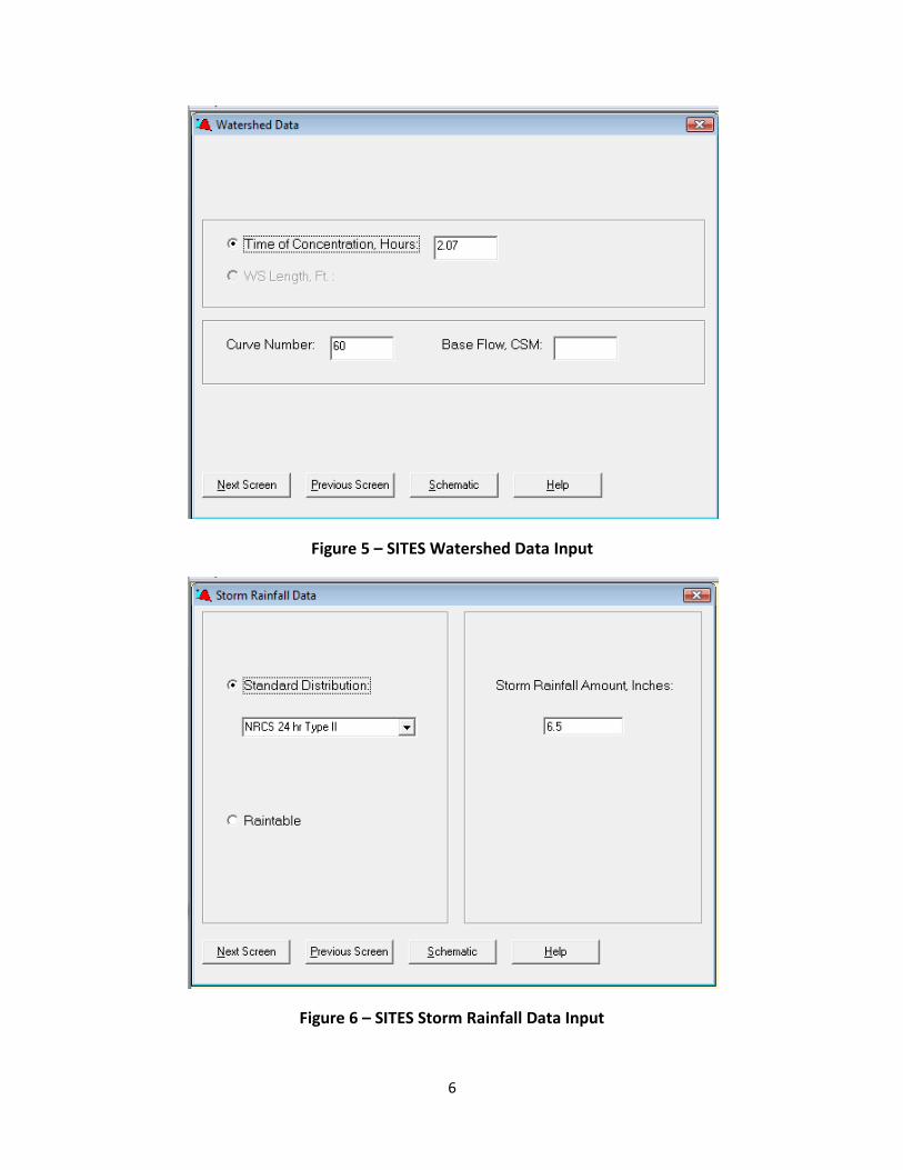
6
Figure 5 – SITES Watershed Data Input
Figure 6 – SITES Storm Rainfall Data Input

7
The program works by first taking the design storm rainfall amount and distributing the
total rainfall according to several pre-programmed distributions. A map that shows the
different rainfall distributions that should be used in the United States is presented below in
Figure 7. For this study, the type II distribution was selected because Sanderson is located in a
region in this figure that corresponds to this distribution. The next step is then to take the
design rainfall (taken from Figure 8) and subtract the losses that will occur due to infiltration.
This is done by using the SCS method for abstractions. In this method, a dimensionless curve
number that is dependent on basin characteristics is used to calculate the amount of excess
rainfall that will produce runoff. For this study a curve number (CN) of 60 was used for all of the
basins. This is due to a report presented by Hailey and McGill (1983) in which the authors
suggest that in West Texas the AMC I condition or a CN of 60, whichever is greater, should be
used. A map showing the CN alterations in Texas, based on the research by Hailey and McGill
(1983), is presented below in Figure 9. The NRCS, during the design of the dams, had
determined that the CN for the area should be 74. In order to convert this to the AMC I
condition, an equation from Applied Hydrology by Chow, Maidment , and Mays (1988) was
used. An example calculation is shown below. This calculation shows that the CN adjustment
would be less than 60. According to Hailey and McGill, a CN value of 60 should then be used.
𝐶𝑁 𝐴𝑀𝐶𝐼 =4.2𝐶𝑁 𝐴𝑀𝐶𝐼𝐼
10 − 0.058𝐶𝑁(𝐴𝑀𝐶𝐼𝐼)=
4.2 ∗ 74
10 − 0.058 ∗ 74= 54.45
With the excess precipitation known it is then possible to develop a runoff hydrograph based on the watershed area and time of concentration using the SCS hydrograph method.
Figure 7 – Approximate boundaries for NRCS rainfall distributions (USDA, 1986)
Sanderson Watershed
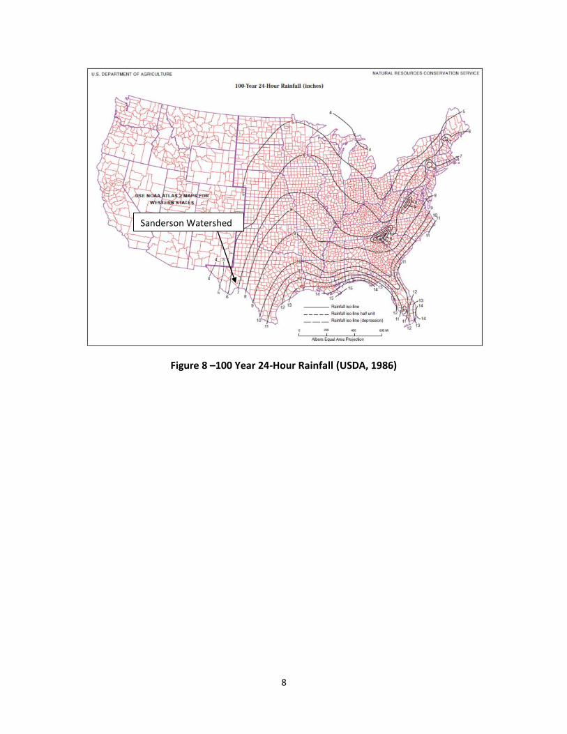
8
Figure 8 –100 Year 24-Hour Rainfall (USDA, 1986)
Sanderson Watershed
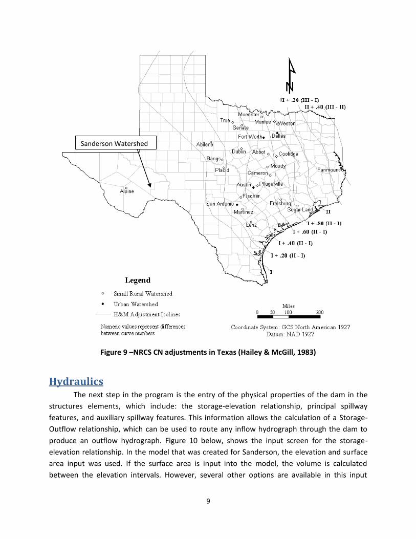
9
Figure 9 –NRCS CN adjustments in Texas (Hailey & McGill, 1983)
Hydraulics The next step in the program is the entry of the physical properties of the dam in the
structures elements, which include: the storage-elevation relationship, principal spillway
features, and auxiliary spillway features. This information allows the calculation of a Storage-
Outflow relationship, which can be used to route any inflow hydrograph through the dam to
produce an outflow hydrograph. Figure 10 below, shows the input screen for the storage-
elevation relationship. In the model that was created for Sanderson, the elevation and surface
area input was used. If the surface area is input into the model, the volume is calculated
between the elevation intervals. However, several other options are available in this input
Sanderson Watershed

10
screen. Another option is to simply input the storage volume at each elevation. Also, direct
input of the storage outflow relationship can be entered. If this relationship is not known,
however, several additional screens follow that allow the calculation of the Storage-Outflow
relationship.
Figure 10 –Storage-Elevation Input Screen
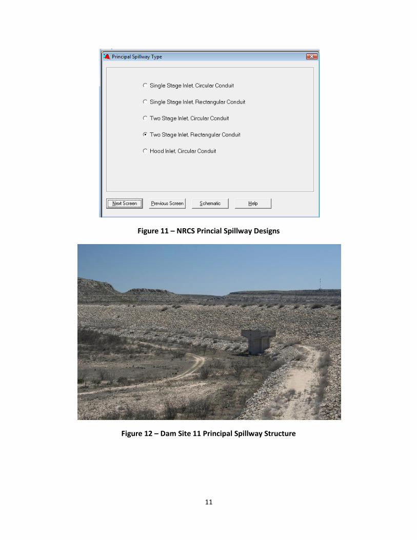
The first step in calculating the Storage-Outflow relationship is to select the principal
spillway design that is at the site. The NRCS has five pre-programmed design types built into the
SITES program. The different types are typical structures that the NRCS uses. Since this project
involves evaluating NRCS dam sites this is not a problem, however this limits the program to
being used in the evaluation of NRCS structures. In Figure 11, presented below, it is possible to
see the different design options. In this project, the Two Stage Inlet Rectangular Conduit design
was used at Dam Site 11 and the Two Stage Inlet Circular Conduit design was used for all the
other structures. For these design types, Two Stage Inlet means that there are two different
inflow devices at two different elevations, and the conduit is the discharge pipe that takes
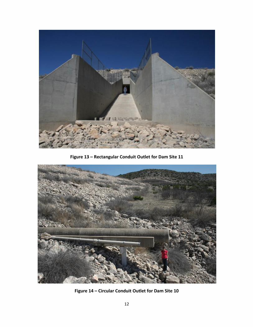
principal spillway inflow and routes it through the dam. Figures 12 and 13 presented below
show the principal spillway structure and rectangular conduit outlet for Dam Site 11. Also,
presented in Figure 14 is a circular conduit used in Dam Site 10.
11
Figure 11 – NRCS Princial Spillway Designs
Figure 12 – Dam Site 11 Principal Spillway Structure
12
Figure 13 – Rectangular Conduit Outlet for Dam Site 11
Figure 14 – Circular Conduit Outlet for Dam Site 10
13
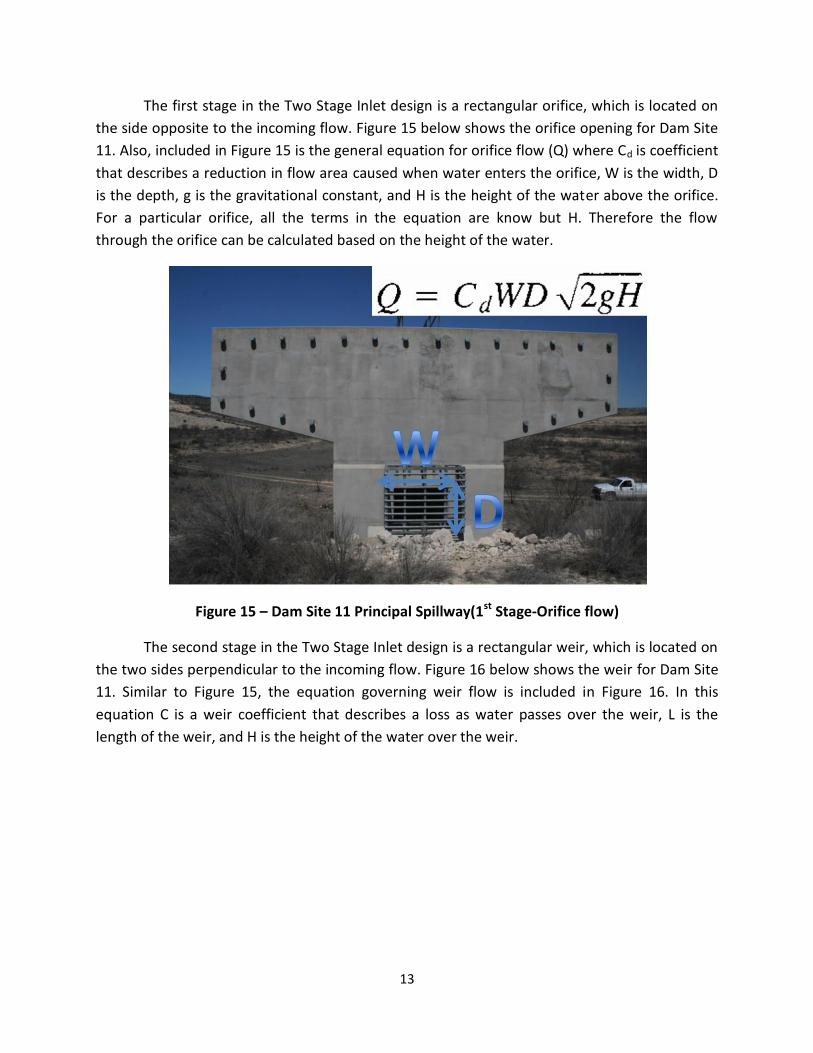
The first stage in the Two Stage Inlet design is a rectangular orifice, which is located on
the side opposite to the incoming flow. Figure 15 below shows the orifice opening for Dam Site
11. Also, included in Figure 15 is the general equation for orifice flow (Q) where Cd is coefficient
that describes a reduction in flow area caused when water enters the orifice, W is the width, D
is the depth, g is the gravitational constant, and H is the height of the water above the orifice.
For a particular orifice, all the terms in the equation are know but H. Therefore the flow
through the orifice can be calculated based on the height of the water.
Figure 15 – Dam Site 11 Principal Spillway(1st Stage-Orifice flow)
The second stage in the Two Stage Inlet design is a rectangular weir, which is located on
the two sides perpendicular to the incoming flow. Figure 16 below shows the weir for Dam Site
11. Similar to Figure 15, the equation governing weir flow is included in Figure 16. In this
equation C is a weir coefficient that describes a loss as water passes over the weir, L is the
length of the weir, and H is the height of the water over the weir.

14
Figure 16 – Dam Site 11 Principal Spillway(2nd Stage-Weir flow)
The Principal Spillway input screen for Dam Site 11 is presented below in Figure 17. In
this screen the inputs for the orifice and weir can be entered. Also, it should be noted that the
Entrance Loss Coefficient Ke is the same as the Cd and C terms in Figures 15 and 16.
Figure 16 – Principal Spillway Input Screen

15
The next input for the structures element is for the Auxiliary Spillway. Figures 17 and 18
show the cross-section and profile, respectively for Dam Site 11. Using the direct entry of
auxiliary spillway coordinates option in SITES gives two inputs for entering this data.
Figure 17 – Dam Site 11 Auxiliary Spillway Cross-Section
16
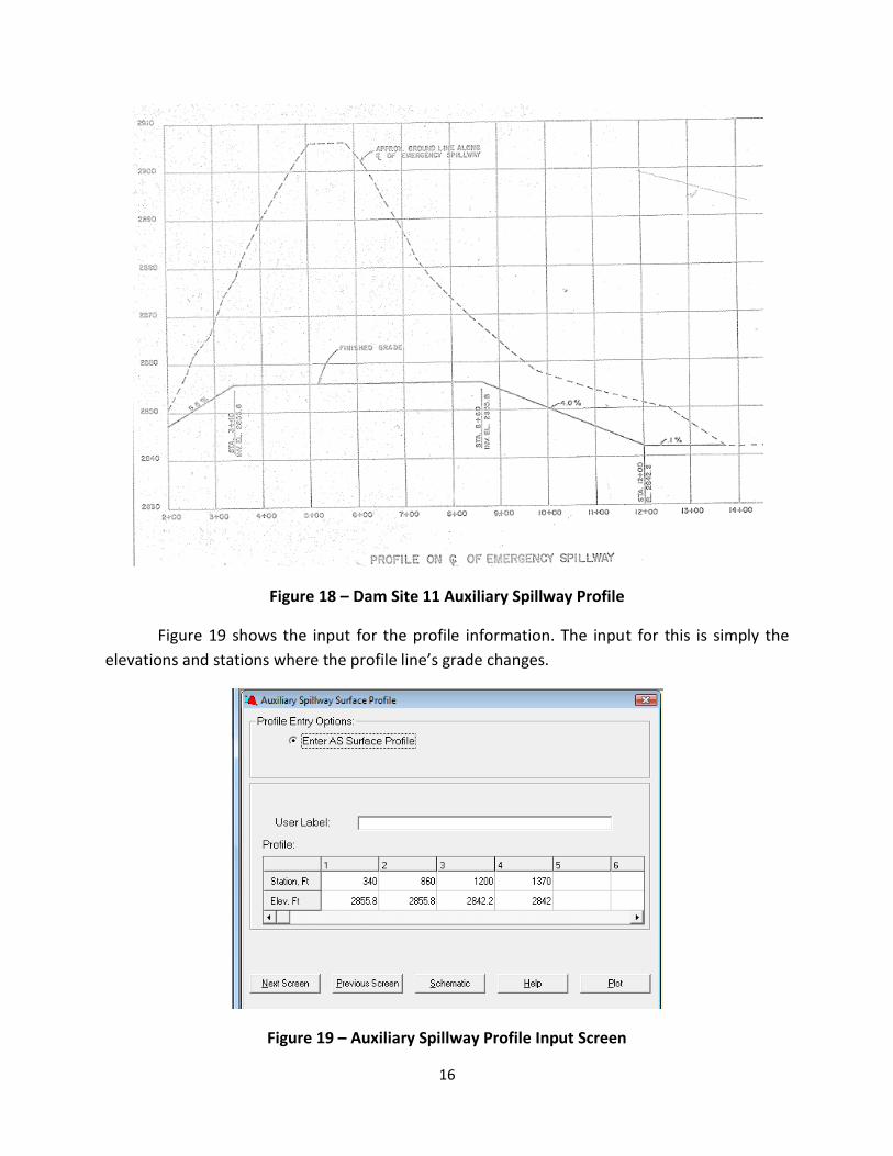
Figure 18 – Dam Site 11 Auxiliary Spillway Profile
Figure 19 shows the input for the profile information. The input for this is simply the
elevations and stations where the profile line’s grade changes.
Figure 19 – Auxiliary Spillway Profile Input Screen

17
Figure 20 shows the input for the cross-section data for Dam Site 11. Only two entries
are needed in this screen, the bottom width and side slope.
Figure 20 – Auxiliary Spillway Cross-section Input Screen
These entries make it possible to calculate to flow through the auxiliary spillway with
Manning’s Equation. Like the equations for weir and orifice flow used in the principal spillway
calculations, Manning’s Equation is also dependent on the water height. This is because the A
(area) and R (hydraulic radius) are functions of the water depth.
-Manning’s Equation
It is important to notice that all the equations governing the flow through the spillways
depend on the height of the water to calculate the flow rate. This means that a certain water
elevation in the dam will produce a given flow rate through the spillways. With the elevation-
storage relationship it is then possible to relate storage with outflow. An example of this
relationship for Dam Site 11 is shown below in Figure 21. The red boxes in this figure outline the
total outflow and volume of storage that occurs at different water elevations in the dam. With
this information it is then possible to perform the hydraulic routing through the dam, given an
inflow hydrograph.
2/13/2 SARn
kQ

18
Figure 21 – SITES Output File for Dam Site 11
River Routing The CONVEX method was used to route the flow from both the upstream uncontrolled
watersheds and structures in Sanderson Model. More information on this method can be
ascertained by reading the National Engineering Handbook, Section 4 Hydrology (Mokus, 1972).
The CONVEX routing method has a single routing coefficient which can be estimated from an
empirical relationship with flow velocity. The original study done by the NRCS had already
calculated the velocities for each reach, so using these numbers I was able to calculate the
19
coefficient based on the following equation given by Mokus, 1972, where V is
the river velocity.
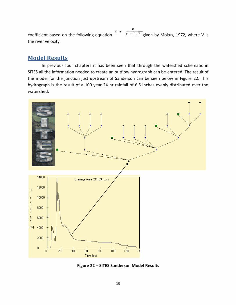
Model Results In previous four chapters it has been seen that through the watershed schematic in
SITES all the information needed to create an outflow hydrograph can be entered. The result of
the model for the junction just upstream of Sanderson can be seen below in Figure 22. This
hydrograph is the result of a 100 year 24 hr rainfall of 6.5 inches evenly distributed over the
watershed.
Figure 22 – SITES Sanderson Model Results
20
Conclusions The NRCS Sites program is a great tool for evaluating a watershed that has flood control
dams. Through the watershed schematic it is possible to create a model that can predict an
outflow hydrograph from multiple uncontrolled and controlled watersheds. Also, the program
can be used to get the storage-outflow relationship for each structure. The drawbacks are that
there are only a limited number of options for the design of the principal spillway and that
SITES is not a Federal Emergency Management Agency (FEMA) approved program to perform
floodplain analysis. However, the information that was obtained through this program on the
storage-outflow relationship is extremely valuable in another model created in HEC-HMS, which
is an approved FEMA hydrology model.
Works Cited Chow, V., Maidment, D., & Mays, L. (1988). Applied Hydrology. McGraw Hill.
Hailey, J., & McGill, H. (1983). Runoff curve number based on soil-cover complex and climatic
factors. Proceedings 1983 Summer Meeting ASAE. Montana State.
Mokus, V. (1972). National Engineering Handbook, Section 4 Hydrology.
USDA. (1986). TR-55 Urban Hydrology for Small Watersheds. USDA.


![Small Dams Project (Loan 750-PAK[SF])](https://static.fdocuments.in/doc/165x107/577ce4191a28abf1038db126/small-dams-project-loan-750-paksf.jpg)