Ternary Line Codes and their Efficiency

Bachelor Thesis by Thomas SchellekensJune 2007.

An early example of a line code: Morse code. From the British Admiralty's Handbook of Signalling, 1913.

AbstractWe collect and describe eleven ternary line codes from the literature, describe the

criteria of line codes in general, and try to make a comparison of the selected line codes. We investigated the effect of runlength and digital sum variation constraints on the

efficiency of a line code. Using previous research, we were able to obtain an exact result of the effect of runlength constraints on the efficiency. We made an approximation using an automated program of the effect of digital sum variation constraints on the efficiency. For the selected codes, the effect of runlength constraints on the efficiency is small. The digital sum variation constraints have a larger impact, resulting in a theoretical maximum

efficiency of 63% for a digital sum variation of 1, saturating to > 95% theoretical maximum efficiency for digital sum variation values of 5 and higher. In general, the more constrained a code is, the less efficient it is. Good trade­offs have to made between

efficiency and runlength and dsv constraints.

At the Chair for Design and Analysis of Communication Systems (DACS) at the University of Twente, the Netherlands.Supervised by Dr. Ir. Pieter-Tjerk de Boer

2

Contents

1. Introduction to the assignment 31.1 Original and adjusted goal of this bachelorassignment 31.2 General structure of the text 4

2. Introduction to line coding 42.1 Definitions 42.2 Introduction 52.3 Two Approaches to line coding 6

3. Criteria for line codes 63.1 DC Component 63.2 Digital Sum Variation 63.3 Clock Recovery 73.4 Efficiency 73.5 Cost/Complexity 83.6 Spectrum 8

4. Coding techniques from the literature 94.1 Linear Coding 9

4.1.1 Precoded linear codes 114.2 Non­linear Coding 11

4.2.1 Alphabetic Coding 114.2.2 Non­alphabetic Coding 13

4.3 Other and mixed codes 144.3.1 PR4 144.3.2 MLT­3 15

4.4 General Techniques 164.4.1 Interleaving 164.4.2 Scrambling 16

4.5 Eleven three­level line coding strategies 17

5. Theoretical efficiency under runlength constraints 185.1 Defining theoretical efficiency 185.2 Extending dk runlength definition 185.3 Determining dk­constrained efficiency 195.4 Adjusting dk classifications 20

6. Theoretical efficiency under dsv constraints 226.1 Previous research 226.2 Brute force sequence generation 22

6.2.1 Sequence generation algorithm and parameters 226.2.2 Test results for q = 2 246.2.3 Integer sequence recognition 266.2.4 Proof of convergence 27

6.3 Optimizing calculations 286.4 Efficiency versus dsv results 30

7. Conclusions 327.1 Conclusion and comparison of 11 different line codes 327.2 Discussion 33

8. References 34

3

1. Introduction to the assignment

1.1 Original and adjusted goal of this bachelorassignmentThe original goal and scope of this bachelorassignment were determined during the initial phase in which a rough proposal was fine tuned after several iterations. Originally, there was a proposal for a new type of ternary line code. After doing some research on line coding in general, we came up with the following description and goals.

Description:

A line encoding strategy is the way in which a bitstream is sent over a

certain medium. Depending on the situation, certain requirements must

be met. The criteria whereby a line encoding may be evaluated include

the following:

∙ Presence of a DC component

∙ Ease of clock recovery

∙ Error detection

∙ Efficiency

∙ Cost/complexity

∙ Noise immunity

This assignment will focus on 3­level encoding strategies. This is the

situation where the physical medium is capable of carrying 3 different

signal levels (e.g.. ­1, 0, 1). Examples of such encodings are AMI and

HDB3. These are rich encodings, with possible physical layer violations

allowing framing and error detection, as well as correct clock recovery.

The goals of this assignment are:

∙ Literature search for 3­level encodings.

∙ Design and development of one or more new 3­level encoding strategies,

possibly using precise timing to increase the efficiency.

∙ Comparison of the encodings.

∙ Research to which extent this encoding strategy might be implemented

in a real communication system.

A very important step was to first research the literature regarding the subject of line coding. Once a lead was found it turned out that there was indeed a lot of research about the subject, spanning the period of 1960 onwards, with a lot of research being done in the first 20 years. During the literaturestudy it became clear that the subject of line coding (even when restricted to three level line codes) is broad. Eleven line codes were selected for evaluation, and it became clear that a formal measure of a code’s efficiency was needed. It turned out that the subject of efficiency was quite interesting, and this would become the focus of the remaining part of the assignment. We analyzed one part of the efficiency problem (runlength constraints, see 3.3), and we made an approximation by simulation of the other part of the efficiency problem (direct current constraints, see 3.1).Essentially, this assignment started with a literaturestudy about line coding, then singled out efficiency as the one factor to focus on.

We dropped 2 goals from the assignment:

∙ Design and development of one or more new 3­level encoding strategies,

possibly using precise timing to increase the efficiency.

∙ Research to which extent this encoding strategy might be implemented

in a real communication system.

Since our literature search already provided plenty interesting material for research.

4

The goal that we added can be phrased as:∙ Research the relationship between efficiency and the various constraints of line codes

The adjusted goals of this bachelorassignment are:

· Literature search for 3-level encodings· Research the relationship between efficiency and the various constraints of line codes.

The question that we would like to answer is:

· Do the selected line codes utilize their available efficiency? How (if at all) do they compare with each other?

1.2 General structure of the textIn section 2, the reader will be introduced to line coding and some of the problems encountered. Then, in section 3, we will explain the criteria whereby a line code may be judged.In section 4, the different classes of multilevel coding (with a focus on ternary) strategies will be categorized (largely taken from [4]), the different design choices will be considered and examples will be given. This also includes the eleven line codes that we wish to compare.Section 5 will deal with one aspect of this assignments’ focus on efficiency, efficiency under runlength constraints, starting with previous research but making some extensions as well. Section 6 will deal with the second aspect of the efficiency, efficiency under dsv constraints, and it is here that the larger body of original work is presented, although we again start from previous work. Finally, section 7 will give an overview of the line coding strategies, by means of a table showing how the various line codes score on the efficiency criterion. We will also present some general conclusions. References are provided at the end.

2. Introduction to line coding

2.1 DefinitionsFirst of all, we will give some definitions of the terms used in this text, to avoid confusions. A ¹ superscript symbol defines a generally used term, a ² superscript defines a custom term.

­Line¹: Any signal­carrying medium.­Bitstream¹: The incoming/outgoing sequence of ones and zeroes from/to the upper layers

(with respect to the OSI reference model). The to­be­encoded and decoded sequence of bits, with no reference to what they represent (e.g. packets or connections).

­Linestream²: The bitstream in its encoded form, as it is sent over the line, after applying the line coding.

­Line coding¹: The term now used for the technique whereby the bitstream is converted to the linestream. Sometimes also called "Pulse Transmission Plan" or "Transmission Code". A particular way of line coding can be called a line coding strategy, but because it (and the others) are a mouthful and the term has to be used regularly throughout the text, we shall sometimes just refer to “a line code” or “code” instead.

­Baudrate¹: The rate at which signals (either binary, ternary, or N­ary) can be sent and recovered over the line.

­Bitrate²: The speed at which information is transferred from sender to receiver, the “net speed” as perceived by the upper layers.

5

2.2 IntroductionLine coding is the mapping of the bitstream onto the physical signals. It is part of the physical layer in the OSI reference model.For example, if we represent a logical 0 by zero voltage, and a logical 1 by 5 volt, a bitstream of 0 0 1 1 0 1 0 1 would translate to 0 0 5 5 0 5 0 5, see figure 1.

Figure 1: The mapping of a bitstream on the voltage levels

Line coding is an agreement, a protocol in the sense that we have a limited set of symbols (in our case, line voltages) with a fixed meaning.

The bitstream in its raw form may consist of any sequence of zeroes and ones. If one tries to send them over a line in this “straight” or “direct” form, several problems occur.

One of these problems is that the average signal value (voltage level) is directly dependant on the particular bitstream. In one case, you could have an average signal value of 0.2, and in a different case it could be 0.8. Why exactly that is a problem is explained in section 3.1.Another problem is that arbitrarily long sequences of a particular symbol in the bitstream would result in arbitrarily long sequences of a particular symbol in the linestream. This would cause problems for the receiver, which has to extract the clock speed the sender is operating to from the linestream itself, and that would become problematic if there are no transitions in the signal (just that single symbol). This is elaborated further upon in section 3.3

Other factors that play an important role are properties of the physical line (the available frequency spectrum) or limits on electromagnetic radiation, specified by the FCC (a regulatory government agency).Furthermore, we are usually able to differentiate between many signal levels on a physical level (not just two, as in the example above). In this assignment we will focus on three­level codes, that is, we have three levels available for transmission. The reason one can not just use any number of symbols is that differentiating between these symbols becomes increasingly harder as more symbols are used within the amplitude range. More symbols means smaller differences between them (for example, if signal levels ­1, 0 and 1 are used for 3 level encoding, a 21 level encoding would require ­1, ­0.9, ­0.8, etc).When that happens, the distortion from transmission (the signal­to­noise ratio) starts limiting the number of different symbols that can be used.In practice, three­level codes are often encountered.

6

2.3 Two approaches to Line CodingTo tackle some of the most important issues in Line Coding (briefly described in the previous subsection) two different approaches can be used [3]:

­Use more than 2 signalling levels on the line, while keeping the baudrate the same (as with binary signalling). (Effectively allowing more information)­Make the baudrate greater than the bitrate. (Idem)

The result of these techniques is that some redundancy (superfluous, added, repeated information) is introduced in the line coding strategy. This little extra information allows for certain constructions that address some of the problems with line coding, as we will see later. An example of the second technique is Manchester Encoding. We will focus on the first technique.

3. Different evaluation criteria [4], [5]The criteria whereby a line coding strategy may be evaluated include the following. Examples of application of these criteria will show up in section 4.

3.1 DC ComponentA DC Component refers to the presence of an average transmitted current that is not zero. The average signal level consists of the sum of the symbols used to represent the ones and zeroes over a certain period of time. If one would just use “straight” line coding (encode a zero as zero and a one as one), the average of that signal is directly dependant on the particular bitstream it is encoding. For example, a bitstream consisting of 96 zeroes and 32 ones has a different average signal than a bitstream consisting of 64 zeroes and 64 ones, namely, 0.75 versus 0.5. The received signal is considered to be zero if it is below some value and one if it is above that value (usually called a threshold), and this threshold is usually derived from the average signal value. For example, if the average signal is 0.5, the thresholds might be 0.5. So a signal is decoded as zero when it is lower than 0.5 and one if its higher.However, this means that changes in this average signal may lead to erroneous decisions about what are zeroes and what are ones. Let’s say the bitstream happens to consist almost entirely of ones over a particular period in time. That would mean the average transmitted signal would be close to 1, too. If the threshold would be derived from that value, it would also be set to 1. Since a signal higher than 1 is never transmitted, ones are never received in that case.This problem is usually referred to as baseline wander or dc wander. The average transmitted signal is often called dc content, dc component, or low­frequency content.Another problem with a DC component is that common electrical components (as used in transmitting and receiving equipment) can not handle it. Long range transmission usually also does not pass a DC component [19].

3.2 Digital Sum Variation.When there is no DC component (the average transmitted signal is zero), a Digital Sum Variation can be defined (dsv). The digital sum is the sum of transmitted symbols so far. If we transmit 0 ­ ­ ­we have a digital sum of ­3. If we transmit 0 ­ + + ­ + 0 +, we have a digital sum of 2. In the string 0 ­ + + ­ + 0 + we have a maximum of 3. Likewise, the string has a minimum, which is ­1, if we sum the first 2 symbols.The difference between the largest digital sum and the minimum digital sum is the Digital Sum Variation (dsv). It is the largest possible distance between two digital sums in a string of symbols.In other words, to find the dsv of a particular line coding, one comes up with the minimum digital sum and the maximal digital sum (starting at any one symbol) and calculates the difference. A dsv can be defined when there is a DC component, but it is infinite (since arbitrarily long sequences of + can occur, as well as arbitrarily long sequences of ­, which results in an infinite maximum and/or minimal digital sum.)

7

In other literature, one can also encounter a number which is defined like “number of allowable digital sum states”. This is the same as the dsv plus one. (2 allowable states is a variation of 1, 3 allowable states is a variation of 2, etc.)

We might have no DC component, but still have a temporary average signal (over the course of a few symbols). The dsv gives us a measure for that temporary amount of low­frequency power [18, 10] and a measure for the amount of distortion a signal suffers [4].

3.3 Clock RecoveryFor the linestream to be decoded correctly into the bitstream, the analog signal received must be sampled to a digital signal at constant time intervals. The sender and receiver agree upon the speed at which they send/receive (enabling the sampling). However, a sender and receiver can never operate at exactly the same speed. Also, some bits might be packed a little closer together than others (jitter, due to physical causes, for example, differences in temperature). The result of this is that the receiving side has to constantly adjust itself to the phase of the linestream to decode it properly. With a receiver that has to constantly adjust itself, a long row of identical symbols may cause problems, because there are no transitions in the received signal that the receiver can synchronize its phase upon. Therefore, there must be a certain number of transitions in the signal, and a limit must be placed on the maximum number of identical symbols in a row. This limit can be guaranteed by the line coding itself (the limit is inherent in the coding rules), or one could use bit stuffing. Bit stuffing essentially is inserting (“stuffing”) an extra zero bit into the bitstream when a maximum number n of one bits is reached (vice versa for long rows of zeroes). Say we choose the maximum n = 5, then any sequence containing 5 1’s would have an extra 0 appended at the end of that string. The receiver would automatically remove any zero that follows 5 ones in a row, thus recovering the original, non­stuffed, sequence. Whether the runlength limit is part of the code design or if it is a result of bit stuffing, it results in a maximum runlength limit. In fact, not only a maximum runlength, but also a minimum runlength can be specified. We name these minimum and maximum runlength d and k constraints, or dkconstraints. For example, if we have no minimum runlength, and a maximum runlength constraint of 6, we have a dk=0,6 code. We elaborate on runlength constraints in section 5. Minimum runlength constraints are sometimes used to limit intersymbol interference.

3.4 EfficiencyTo be able to make guarantees about the previous 2 criteria, mechanisms are introduced that include extra information (e.g. extra transitions for the receiver to synchronize upon) in the transmitted symbols. These cause a decreased efficiency (bitrate) of the line coding strategy, because the extra information they send takes up some portion of the transmission capacity.

The efficiency of any line coding strategy can be measured as the extent to which it attains the theoretical maximum speed of the channel. We define theoretical maximum speed of a channel as the channels symbol rate (baudrate) multiplied by the information capacity per symbol (from now on measured in bits). We will set this theoretical maximum speed to 1, and measure the efficiency of any line code as a fraction of one.For the theoretical maximum speed of a channel, any symbol is allowed to follow any other symbol, there are no constraints regarding illegal sequences of symbols. We will see later that we often do want to constrain the possible allowed sequences (for the sake of clock recovery and to keep the dsv within limits), and construct line codes that do exactly this. These line codes therefore do not attain the channels theoretical maximum speed.

Before defining our measure of the efficiency of a line code, we first need a measure for information content.

The theorem about the information content of a message (symbol) occurring with a certain probability is formulated by Shannon as I(M) = ­Logp(M). M is the probability of occurrence of a message from a certain number of available messages (the message space). P, the base of the

8

Log, is usually 2, meaning the information content is measured in bits. ­ Logp(M) equals Logp(1/M), so if the chance of a certain ternary symbol occurring is 1/3, the information content is of any ternary symbol is Log2(3), measured in bits. That is, a ternary symbol contains 1.58 bits.In general, Log2(M) is the bit/symbol rate for a M­ary symbol.

We can also use this concept for sequences of symbols. If we have the set of all possible ternary sequences of length 3 (27 different sequences), we can view a single sequence as a single symbol out of an alphabet of 27 symbols. Indeed, Log2(27) is 4.76, 3 times the binary information content of a ternary symbol (1.58), so one symbol out of our set of 27 symbols coincides with the same information content of 3 ternary symbols.If we only use 25 sequences out of all 27 sequences, the information content of a single sequence out of this “constrained” set is not so great as the information content of a single sequence out of the “unconstrained” set of 27 sequences. It is only Log2(25). And if we divide this by Log2(27), we normalize this to a fraction. For example, say we don’t want to allow the sequences + + + and ­ ­ ­. This means we have an efficiency of Log2(25)/Log2(27). That is an efficiency of 0.9677, the drawback of constraining our sequence set.

This fraction, Log2(number of possible sequences)/ Log2(number of useable sequences) will be the measure of efficiency we will be using. We distinguish between 2 cases. In one case, we are only able to calculate the number of useable sequences for a given finite sequence length, and we have only an approximation. In the other case, we are able to calculate the results for infinite sequence length, and we have an exact result. Other literature sometimes refers to this last case as the “asymptotic information rate”.

3.5 Cost/ComplexitySome techniques might be very useful, but the implementation details might render them inadequate anyway. Vice versa, a technique might not seem very good but the simplicity of design may cause it to prove useful in a particular application. Analysis of a circuit’s complexity for a particular line code is out of the scope of this assignment, but we can usually make an educated guess, mostly based on whether it is linear (see section 4.1). The authors of [18] do deal with this subject.

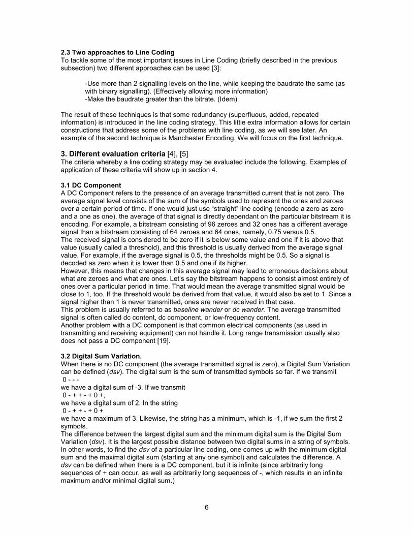
3.6 SpectrumSpectrum refers to the range of electromagnetical waves used to send and receive signals on the physical medium. Every medium that is used to carry such signals has a limited frequency spectrum. For example, only frequencies between 300 and 900 Hertz may be available. Any line coding strategy has a characteristic power spectrum, which can be represented by a graph of the power (vertical) plotted against the frequency (horizontal). Certain constraints caused by choosing a certain medium (and corresponding spectrum) are therefore important when designing or evaluating a useful line coding strategy.Though the spectrum is an important criterion, we will leave it at this because it is an electrotechnical story for the larger part. Figure 2 (from [4]) is the power spectrum of Twinned Binary.

Figure 2: the power spectrum of twinned binary.

It is interesting to see that the spectral density is practically zero at low frequencies. This meansthat this line coding strategy does not have a DC component (which, quite obviously now, is sometimes referred to as low frequency content)

9

4. Different techniques [4]

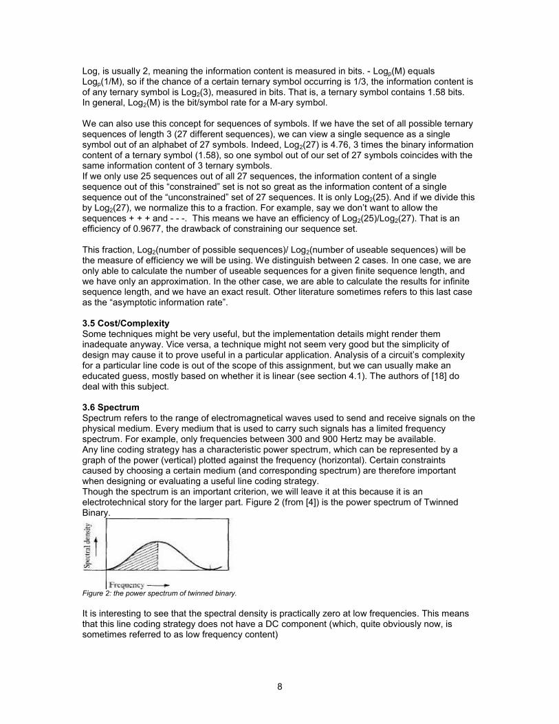
4.1 Linear CodingWhen a stream of bits is linearly encoded, it means that it is encoded in such a way that the linestream is the result of the sum (a linear operation) of 2 (or more) individual waveforms that represent these bits.The mathematical definition of a linear code is:

n! = !"

#

K

kkkn

0

"#

The left part of the equation, n! is the resulting ternary code level (­, 0 or +) for bit n.

The right part consists of a summation from zero until K, where kn## represents one particular

bit from all the binary data, and multiplied with k" represents its coded form.

So the result of the summation until K of kkn "# # is the coded form of the bit n, n! .To see how this works, let’s take a look at a basic linear coding strategy, twinned binary. In twinned binary, a zero !"#$%&$%"%'(%)#*"#"!'+,-#.!(/#,#0#122342#5#6'%#!"#$%&$%"%'(%)#*"#­sin(x).So zero = 0" = sin(x) (lambda­element zero), and one = 1" = ­sin(x) (lambda­element one).Summing these waveforms for the bitstream 00110001 results in 0 1 0 ­1 0 0 1 (8 bits now become 7 bits because no bit precedes the first bit, causing an undefined summation.) This is presented graphically in figure 3.

Figure 3: The summation of individual lambda­elements in twinned binary.

10

This technique is attractive for its simplicity (of design and signal recovery) [4]. Twinned binary has no DC component, and a DSV of 1.Decoding is now done by subtracting the previous lambda element from the current lambda element. Figure 3 can be understood using the following rule: “For every positive pulse, decode a transition from zero to one, for every negative pulse, decode a transition from one to zero, and for every zero pulse, decode a one if the last transition was to one, and a zero if the last transition was to zero”.

This arrangement can cause error propagation, meaning one error results in a stream of errors. For example, when a 1 in a linestream is interpreted as a zero (e.g. because of noise), instead of a transition to ones, all the succeeding zero pulses are decoded as being zeroes. This problem is addressed in subsection 4.1.1.

Another example of a linear code is duobinary.Figure 4 present a picture much like figure 2 to explain duobinary. It differs in the value of the lambda elements (from the definition of a linear code).

Figure 4: The summation of individual lambda elements in duobinary

Once again, there are 7 symbols instead of 8, this is because transitions are encoded.Duobinary has a DC component (and infinite dsv), and also the possibility of long rows of a single symbol, making clock recovery hard.

11

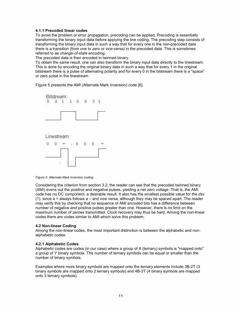
4.1.1 Precoded linear codesTo avoid the problem or error propagation, precoding can be applied. Precoding is essentially transforming the binary input data before applying the line coding. The precoding step consists of transforming the binary input data in such a way that for every one in the non­precoded data there is a transition (from one to zero or vice­versa) in the precoded data. This is sometimes referred to as change­of­state encoding.The precoded data is then encoded in twinned binary.To obtain the same result, one can also transform the binary input data directly to the linestream. This is done by encoding the original binary data in such a way that for every 1 in the original bitstream there is a pulse of alternating polarity and for every 0 in the bitstream there is a "space" or zero pulse in the linestream.

Figure 5 presents the AMI (Alternate Mark Inversion) code [6].

Figure 5: Alternate Mark Inversion coding

Considering the criterion from section 3.2, the reader can see that the precoded twinned binary (AMI) evens out the positive and negative pulses, yielding a net zero voltage. That is, the AMI code has no DC component, a desirable result. It also has the smallest possible value for the dsv (1), since a + always follows a – and vice versa, although they may be spaced apart. The reader may verify this by checking that no sequence of AMI encoded bits has a difference between number of negative and positive pulses greater than one. However, there is no limit on the maximum number of zeroes transmitted. Clock recovery may thus be hard. Among the non­linear codes there are codes similar to AMI which solve this problem.

4.2 Non-linear CodingAmong the non­linear codes, the most important distinction is between the alphabetic and non­alphabetic codes.

4.2.1 Alphabetic CodesAlphabetic codes are codes (in our case) where a group of X (ternary) symbols is "mapped onto" a group of Y binary symbols. The number of ternary symbols can be equal or smaller than the number of binary symbols.

Examples where more binary symbols are mapped onto the ternary elements include 3B­2T (3 binary symbols are mapped onto 2 ternary symbols) and 4B­3T (4 binary symbols are mapped onto 3 ternary symbols).

12

This way, an increased bitrate becomes possible (assuming ternary symbols can be send at the same speed). This increase is theoretically 1.58, Log2(3). This is a result of the fact that a ternary symbol holds more information than a binary symbol (since the likelihood of occurrence of a specific ternary symbol is smaller). The 3B­2T and 4B­3T codes achieve this increased bitrate.3B­2T even reaches 95 percent of the theoretical limit [4], but has the drawback it introduces a DC component. Since there are 8 3­bit symbols, and 9 2­ternary symbols, one can be left out. When this symbol is chosen to be 00, the ++ and ­ ­ symbols are still used, causing the possibility for an infinite dsv and hard clock recovery.4B­3T is less effective, but has the advantage it does provide a zero DC voltage, and places a limit on the maximum number of equal symbols transmitted in a row (for clock recovery). We will now use MS43 [8] as an example. MS43 is a 4B­3T encoding (in the sense that it translates 3 ternary characters to 4 binary characters), but has a better dsv than other 4B­3T encodings [4]. MS43 does this by examining the sum of all transmitted characters, and based on that information it decides which character it should assign to the next 4 bits. This is called state­dependent encoding.The table for MS43 is presented in figure 6. (taken from [8])

Binary Sequence Digital Sum1 2 or 3 4

0000 +++ ­+­ ­+­0001 ++0 00­ 00­0010 +0+ 0­0 0­00100 0++ ­00 ­001000 +­+ +­+ ­­­0011 0­+ 0­+ 0­+0101 ­0+ ­0+ ­0+1001 00+ 00+ ­­01010 0+0 0+0 ­0­1100 +00 +00 0­­0110 ­+0 ­+0 ­+01110 +­0 +­0 +­01101 +0­ +0­ +0­1011 0+­ 0+­ 0+­0111 ­++ ­++ ­­+1111 ++­ +­­ +­­

Figure 6: The MS43 encoding/decoding table

When a sequence has to be transmitted, the digital sum is calculated and brought to one of the 4 states by choosing the corresponding sequence. Of course, the trade­off here is that this coding strategy is more difficult to implement, because the digital sum has to be monitored.The dsv of MS43 is 5. There are 4 different end­states for the digital sum, however, there can be temporary larger (and smaller) values for the digital sum, for example, if 0110 (+ ­ 0) is transmitted and the digital sum is 4, it temporarily becomes 5. And if the digital sum is 1, and 0110 is transmitted (­ + 0), the digital sum temporarily becomes 0. So we have possible states for the digital sum, and thus a variation of 5.Another example of state­dependent encoding is Paired Selected Ternary (PST).The translation table for PST (from ternary to binary symbols) is presented in figure 7.

Figure 7: The PST encoding/decoding table

Ternary Binary­ + 00

0 + or 0 ­ 01+ 0 or ­ 0 10+ ­ 11

13

PST can maintain a zero voltage level. PST does this by switching between 2 states. In one state, 0 + and + 0 are used for 01 and 10, respectively. The other state uses 0 – and – 0 for those binary sequences. After every occurrence of 01 or 10, it switches to the other state, ensuring the zero voltage. Let’s look at an example of a PST encoded bitstream: (where | denotes a state switch)

Bitstream: 00 01 10 01 11 00 11 01 10PST encoded linestream:–+ 0+ –0 0+ +– –+ +– 0– +0 | | | | |

In general, PST has a digital sum variation of 3. Specifically, this happens when– +, 0 +, + – is transmitted. We then have a digital sum of ­1, 0, 0, 1, 2, 1. There are 4 states, so the variation is 3.

4.2.2 Non-alphabetic CodesNon­alphabetic codes are usually of the "filled bipolar" type. These codes use bipolar signalling (i.e. operate like AMI, see section 4.1.1) and are DC­free, but guarantee limited number of zeroes in the linestream (facilitating clock recovery, see section 3.3). These codes are usually marked by the maximum number of consecutive zeroes they allow (e.g. B6ZS, HDB3), which they “fill” with a characteristic sequence of symbols that can be recognized and filtered out by the receiver.Let’s take B6ZS as an example. B6ZS stands for Bipolar 6 Zero Substitution. Like in AMI, zeroes are encoded as zero pulses and ones as pulses of alternating polarity. This ensures consecutive pulses of the same polarity never occur. When a stream of six consecutive zeroes has to be encoded, it is not encoded with the bipolar technique, but a physical layer violation is transmitted. A physical layer violation in this case is a violation of the “alternating polarities” rule. In practice, this means that a string of 6 characters is transmitted that contains some succeeding symbols of the same polarity. This string is designed to keep the digital sum as small as possible. When the receiver receives such a filling sequence it recognizes the consecutive pulses of the same polarity, and knows it has to decode it as a string of 6 zeroes. This is presented graphically in figure 8 (taken from [7]).

Figure 8: B6ZS encoding with a filling sequence at the dashed line.

HDB3 (High Density Bipolar 3) is a very similar technique. When 4 consecutive zeroes are to be encoded, the 4 zeroes are encoded in one of four ways, depending on the digital sum and the previous transmitted mark (an encoded one, a pulse). If the DS is zero and the last transmitted mark was a +, 000+ is transmitted. If the DS is zero and the last transmitted mark was a –, 000–is transmitted (both cause a violation of the alternating polarity rule).If the DS is –1 or 1, then either +00+ or –00– is transmitted, respectively, causing a violation and a switch of DS from –1 to 1 or vice versa.For example, 1 0 1 0 0 0 0 0 1 1 0 0 0 0 1 1 0 0 0 0 0 0Would be converted to + 0 – 0 0 0 – 0 + – + 0 0 + – + – 0 0 – 0 0

14

Figure 9 presents the HDB3 and B6ZS code result for the same bitstream.The digital sum variation for HDB3 is 2, as we have 3 different DS states (the physical layer violations cause a switch of ­1 to 1, plus the DS state one is 3 states.)The digital sum variation of B6ZS is 3, since the DS can have 4 states, starting from symbol 4 these are ­1, ­2, ­1, 0, ­1, 0, 1.In general, this can happen when a filling sequence is transmitted, one regular symbol is transmitted, and another filling sequence is transmitted.

Figure 9: B6ZS and HDB3 code result for the same bitstream.

4.3 Other and mixed codes

4.3.1 PR4The PR4 encoding (Partial Response class 4) is an interesting line coding technique, mainly because it is the line coding strategy selected for use in the Twentenet Local Area Network, from as many as 16 other candidates [9]. The reasons for this choice are primarily the spectrum PR4 generates and the energy distribution therein. PR4 is actually a linear code (as described in [15]), but the use of filling sequences as described in [9] render it non­linear. PR4 (as used in [9]) can be described using 2 formulas.

The precoder: pr(m) = pr(m­2) + SD(m) % 2 (note: X + Y % 2 is equal to X XOR Y, but we will use the

With pr(m) the precoded mth bit notation as used in [9])

SD(m) the mth bit of the bitstream (SD stands for SendData)% the modulo operatorpr(0) and pr(1) defined to be zero.

The line code: linecode(m) = pr(m) – pr(m ­2) (Except in the case of a physical layer violation)With linecode(m) the mth ternary element of the linestream.

Note that to get the first element of the linestream, one starts at 2, so the first element would be given by:

linecode(2) = pr(2) – pr(0)

pr(2) = pr(0) + SD(2) % 2 According to the formula= 0 + 0 % 2 For example, we take SD(2) (the first bit from the

bitstream) to be zero = 0

linecode(2) = 0 – 0 = 0 0 is the resulting ternary element.

One can now verify that the next example bitstream: 0 1 1 1 0 1 0 1 0 0Is converted by the PR4 encoding to 0 1 1­1 0 1 0­1 0 0

15

It can be seen that any 1 in the bitstream is converted to either 1 or ­1 in the linestream, and any 0 in the bitstream is converted to a 0 in the linestream (Bipolar signaling). Thus, a long sequence of zeroes in the bitstream would once again lead to an unacceptable long period without transitions in the linestream. Like other filled bipolar codes, PR4 uses a physical layer violation to ensure transitions in the linestream within a certain period. This is done by replacing a string of Nzeroes in the bitstream with N­3 zeroes followed by 1 0 1. This string of N elements from the bitstream would then be encoded with the formula:

linecode(m) = ­(pr(m) – pr(m­2)) (note the minus sign)

If the bitstream at a certain point would look like, say0 0 0 0 0 0 0 0And N would be chosen 8; this string of 8 symbols would be replaced by0 0 0 0 0 1 0 1And this string would be encoded according to ­(linecode(m) = pr(m) – pr(m­2)), which would result in either 0 0 0 0 0 1 0 ­1 or 0 0 0 0 0 ­1 0 1, depending on pr(m­2) being 1 or 0, respectively.Since the receiver has received the entire bitstream so far, it knows the value of pr(m­2). With this knowledge, it can detect when it receives a 1 0 ­1 when it should have been ­1 0 1 or vice versa. The receiver then knows it has to replace those 3 bits with 3 zeroes. The original bitstream (8 zeroes in a row) is thus correctly received.In the Twentenet Local Area Network, N is chosen to be 5 (an experimental result rather than theoretical optimum). The dsv of PR4 is 2 (3 possible states for the digital sum).

4.3.2 MLT-3Another coding strategy that is difficult to classify is MLT­3, an encoding that cycles through the states – 0 + 0 – 0 + 0 – 0 + 0 and changes to the next state when the bitstream changes from 0 to 1 or vice versa. It also has some features from an alphabetic code, since the bitstream is first encoded with 4B/5B encoding. This is to ensure that there will be sufficient changes in the signal for the clocks to synchronize upon. If 4B/5B were not employed, no change in the bitstream would result in no change in the linestream, an undesirable result (see section 3.3). MLT­3 is described in [12] and used in the 100BASE­TX Ethernet standard, one reason for inclusion.MLT­3 has an infinite dsv and therefore a DC component. For example, the state could change to + and stay there for 3 clock periods (so the symbol + is transmitted 3 times). The DS would then be 3. It could then cycle to 0, –, 0 in 3 clock periods and after that could once again remain + for 3 clock periods. This causes the DS to increase and therefore causes a DC component and infinite dsv. However, the Ethernet standard is used for local area networks, so the DC component does not need to be transferred over long distances.It is interesting to note that the frequency spectrum that MLT3 generates contains less high frequency components then the bitstream it is encoding. The frequency spectrum is first enlarged by using the 4B/5B encoding, from 100 MHz to 125 MHz, but applying the MLT­3 coding cuts it by two to 62.5 MHz. This can intuitively be seen from the fact that the– 0 + 0 – 0 + 0 distance between 2 – symbols or 2 + symbols (which is the wavelength in a physical sense) is 4 symbols, twice as long as the distance for – + – +.

16

4.4 General TechniquesFurthermore, there are 2 general techniques which can be applied to linear and non­linear line coding strategies. These are Interleaving and Scrambling.

4.4.1 InterleavingInterleaving is a technique where a bitstream is divided into 2 (or more) bitstreams, namely that of the odd and that of the even bits (in the case of 2 bitstreams). These 2 streams are then both encoded using the chosen line coding strategy. Its main advantage lies in shaping the frequency spectrum. A drawback is that interleaving can double the dsv.

We now use interleaved bipolar as an example. Here the string 00 11 01 01 00 10 01 10 must be sent. First of all, it is divided in 2 streams, namely the odd and even bit strings. Odd string: 01000101Even string: 01110010These are both encoded using the bipolar technique, starting with a positive pulse for a one.Odd linestream: 0 + 0 0 0 – 0 +Even linestream: 0 + – + 0 0 – 0When these 2 are merged, the linestream 00++0–0+00–00–+0 is the result.One can see that the dsv is now 2 (since 2 consecutive positive or negative pulses can occur)

4.4.2 ScramblingScrambling [2], is a technique that "scrambles" the bitstream in a seemingly random, but recoverable way. The purpose is to make the bitstream more random (remove long rows of one symbol), for example by means of a XOR operation with a previous transmitted bit.Scrambling is sometimes called "randomizing". However, there will always be problematic input sequences that are pretty random when they go in but generate long sequences of a single symbol at the output.The structure of a scrambler and descrambler is presented in figure 10.

Figure 10: A scrambler and descrambler.

Guided scrambling is a technique where for a piece of the bitstream (sourceword) a possible set of codewords is generated. From this set one can choose the codeword in such a way that maximum­runlength constraints on a given communication channel are satisfied. For an elaborate introduction, see [11].

17

4.5 Eleven three-level line coding strategiesWe will now summarize all the coding strategies that we treated in this section. We will try to capture the essential properties in figure 11.First, we list the presence of a DC component and the dsv. If no DC component is present, we list the dsv (since the presence of a DC component makes the dsv infinite).Secondly, we will say whether this line code has a limited number of consecutive symbols (“runlength limited”, essential for clock recovery), and if so, how much.Thirdly, we will say something about how much of the theoretical maximum speed (as defined in section 3.4) this code utilizes. Then, we will characterize each code into one of three classes: Linear, Nonlinear, Nonlinear (alphabetic), and codes of a mixed type. We will not make an explicit judgement of the cost/complexity involved in designing an efficient encoder/decoder for the line codes, but we will just note here that linear codes have simple encoders/decoders [4].

Name DC/DSV Runlength Lim. Efficiency ClassDuobinary Yes / 7 No 0.631 LinearTwin. Binary No / 1 No 0.631 LinearAMI No / 1 No 0.631 Linear (precoded)HDB3 No / 2 Yes/3 0.631 Filled bipolarB6ZS No / 3 Yes/5 0.631 Filled bipolar3B2T Yes / 7 No 0.946 Nonlinear alphabetic4B3T No / 7 Yes/4 0.839 Nonlinear alphabeticMS43 No / 5 Yes/4 0.839 Nonlinear alphabeticPST No / 3 Yes/2 0.631 Nonlinear alphabeticPR4 No / 2 Yes/4 0.631 Mixed bipolar/linearMLT­3 Yes / 7 Yes/4 0.631 Mixed alphabetic/otherFigure 11: Comparison of the eleven three­level line coding strategies

In general, the more constraints we have, the less efficient a code is. The next two sections (section 5 and 6) will focus on this. It will deal with the maximum efficiency under runlength and dsv constraints. This will allow us to make a fairer comparison of the codes, since a very constrained code is inherently more inefficient than a not so constrained code.

18

5. Theoretical efficiency under runlength constraintsTang and Bahl [14] have written a comprehensive article on the efficiency of dk­limited q­nary sequences. The d and k values represent the constraint on the minimum and maximum length of consecutive zeroes between two non­zero symbols. Tang and Bahl have derived formulas for the number of possible sequences given the number of available symbols q in the source alphabet (which is always 3, in our case), the length n of the sequence and the d and k constraints. When the number of allowed sequences is known, it is possible to derive the maximum efficiency of the coding strategy, given these specific constraints. This is shown in more detail later.For every line code we treated, we now try to formulate them in terms of dk constraints (q is always 3 in our case). Then we will determine their theoretical efficiency and compare this to what these codes actually achieve.

5.1 Defining theoretical efficiencyIt is important to have a clear notion of which efficiency we measure as a fraction of which reference efficiency. More background information is in section 3.4

­ The unconstrained theoretical maximum efficiencyWhen any symbol is allowed to follow any other symbol in a sequence of symbols, we say that this sequence is non­constrained. This efficiency is then 1. This is our reference efficiency.

­ The dk­constrained theoretical maximum efficiency.This is the information content of the number of allowed sequences divided by the information content of the total number of sequences. Referencing section 3.4, we see this number is expressed by Log2(useable number of sequences)/ Log2(total number of sequences). The dk­constrained theoretical maximum efficiency is calculated for infinite sequence length, and is therefore an exact result.

­ The attained efficiency.The real­life efficiency of a line code is a fraction of the non­constrained theoretical maximum efficiency.

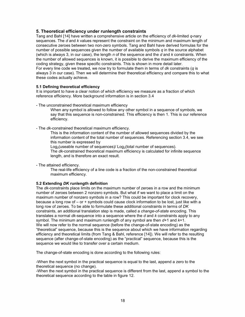
5.2 Extending DK runlength definitionThe dk­constraints place limits on the maximum number of zeroes in a row and the minimum number of zeroes between 2 nonzero symbols. But what if we want to place a limit on the maximum number of nonzero symbols in a row? This could be important for clock recovery, because a long row of – or + symbols could cause clock information to be lost, just like with a long row of zeroes. To be able to formulate these additional constraints in terms of DKconstraints, an additional translation step is made, called a change­of­state encoding. This translates a normal dk­sequence into a sequence where the d and k constraints apply to any symbol. The minimum and maximum runlength of any symbol are then d+1 and k+1. We will now refer to the normal sequence (before the change­of­state encoding) as the “theoretical” sequence, because this is the sequence about which we have information regarding efficiency and theoretical limits (from Tang & Bahl, reference [14]). We will refer to the resulting sequence (after change­of­state encoding) as the “practical” sequence, because this is the sequence we would like to transfer over a certain medium.

The change­of­state encoding is done according to the following rules:

­When the next symbol in the practical sequence is equal to the last, append a zero to the theoretical sequence (no change).­When the next symbol in the practical sequence is different from the last, append a symbol to the theoretical sequence according to the table in figure 12.

19

Practical sequence Theoretical sequenceFrom To Symbol­ 0 +0 + ++ ­ ++ 0 ­0 ­ ­­ + ­Figure 12: Change of state table

The result is that for each practical sequence, we have corresponding theoretical sequence that has a zero for every symbol in the practical sequence that is equal to the previous symbol (a 1on1 mapping). This means that the runlength of zeroes in the theoretical sequence corresponds to the runlength of any symbol in the practical sequence. This means that the dk constraints of the theoretical sequence correspond to the minimum and maximum runlength of any symbol in the practical sequence, which was our goal.

Example:

Practical sequence 0 + 0 0 + + ­ ­ ­ ­ + + + 0 0 ­ ­ 0 +Theoretical sequence + ­ 0 + 0 + 0 0 0 ­ 0 0 ­ 0 ­ 0 + +

Upon studying the above example one can see that the dk constraints in the theoretical sequence (d=0, k=3) translate to a minimum and maximum runlength of d+1 and k+1 for every symbol in the practical sequence.

We will now determine the values of d and k for the various line codes (subtract 1 from the actual minimum and maximum runlength, since these are practical sequences (d+1, k+1) and we actually want to know d and k). The result is presented in figure 13.

Line Code: q: d: k:MLT­3 3 0 3 Duobinary 3 0 7AMI 3 0 7Twinned Binary 3 0 7HDB3 3 0 2PR4 3 0 3 B6ZS 3 0 43B2T 3 0 7MS43 3 0 34B3T 3 0 3PST 3 0 1Figure 13: Change­of­state encoding dk constraints for the eleven line codes

Notes: For PR4, the k value is chosen as used in the Twentenet specification (N=5).In the case of duobinary, no immediate transitions from – to + and vice versa occur.

5.3 Determining dk-constrained efficiencyTang and Bahl give formulae for calculating the theoretical maximum efficiency of a dk­limited q­nary line coding strategy. The above line coding strategies are k­limited, which means that d = 0 and k can have any value. For the k­limited case, the theoretical maximum asymptotic information rate ! = log3("). Here, " is the largest positive root from the characteristic equation Zk+1 – (q­1) [Zk + Zk­1 + … + Z + 1] = 0. Solving for " and ! yields the theoretical maximum efficiency of a line coding strategies with that k constraint. The number of different symbols is represented by q, so always 3 in our case. The results are presented in figure 14.

20

Line Code: DK constrained theoretical maximum efficiencyMLT­3 0.992Duobinary 1AMI 1Twinned Binary 1HDB3 0.975PR4 0.992B6ZS 0.9973B2T 1MS43 0.9924B3T 0.992PST 0.910Figure 14: The dk constrained theoretical maximum efficiencies of the eleven line codes

One can see that when the maximum runlength (k) of a sequence becomes larger (with no constraints on the minimum runlength (d=0)), the theoretical maximum efficiency goes up. This is because of a larger number of available sequences.

However, it might not be a good idea to formulate all codes in terms of change­of­state encoding. We will handle this in the next section.

5.4 Adjusting the dk classificationsIt might be the case that not all line codes need the change­of­state encoding, since some line codes might indeed only have long runs of zeroes, like in the original dk definition.

The coding techniques where the change of state encoding is relevant are:

MS43 (sequences of length 4 of –, + and 0 occur)4B3T (sequences of length 4 of –, + and 0 occur)PST (sequences of length 2 of –, + and 0 occur)MLT­3 (sequences of length 4 of –, + and 0 occur)3B2T (because runs of –, + and 0 occur) (however, the d and k constraints remain the same, namely 0 and 7-Duobinary (because runs of –, + and 0 occur (however, the d and k constraints remain the same, namely 0 and 7-

B6ZS and HDB3 feature only limited long runs of zeroes, so its more precise to formulate these in “straight” dk constraints, namely d=0, k=5 for B6ZS and d=0, k=3 for HDB3.Twinned binary does not feature extended runs of consecutive – or + symbols, however, dremains 0 and k is still infinite.AMI does not feature extended runs of consecutive – or + symbols, however, d remains 0 and k is still infinite.

So we might want to formulate some codes in terms of change­of­state dk constraints, but not all of them, since the dk constrained theoretical maximum efficiency might less accurate.

PR4 (with N=5) is less straightforward to analyze. It has a maximum of 4 zeroes in a row. Runs of consecutive – and + symbols are limited by the fact that a symbol is dependent on previous symbols in such a way that no more than 2 consecutive – or + symbols can occur. Therefore, the zero symbol is not the only symbol with possible extended runlength (4 consecutive zeroes), but its runlength also isn’t equal to the runlength of the other 2 symbols (2 consecutive – or + symbols). This means we can not formulate an exact runlength constraint for all the different symbols.

21

Formulating PR4 in “straight” dk form (d=0, k=4) does not take into account the fact that runs of –and + are limited to length 2. This means that the PR4 encoding is more constrained than this dkformulation represents. This could mean that the calculated theoretical constrained efficiency is higher than it is in reality.The alternative is to formulate in change­of­state encoding. D would be 0 and k would be 4. The runlength of any symbol is now limited to 4 consecutive symbols. This obviously does not take into account that runs of – and + symbols longer than 2 do not occur. Therefore this formulation in dk constraints allows more sequences than the actual PR4 code allows. This means that the calculated constrained theoretical efficiency is higher than what the constrained theoretical efficiency of PR4 should be.We now have 2 possibilities: In the “straight” dk formulation, – and + symbols are not limited at all. In the “change­of­state” formulation, the – and + symbols are limited, but limited until 4, so it still allows sequences which PR4 does not allow. We want to choose that formulation which is the “tightest”, that is, the one that resembles the actual PR4 encoding as closely as possible and yields a constrained theoretical efficiency that is as close to the actual PR4 encoding as possible. Intuitively, this is the “change­of­state” formulation, since the number of sequences that are allowed by this formulation but not by the actual PR4 encoding (sequences with – or + symbols of length > 2 and smaller or equal to 4) is finite, but the number of sequences the “straight” dkformulation allows that are not allowed by the PR4 encoding is infinite (sequences with – or + symbols of length > 2).We can verify this by entering the dk values in the equation.D=0, K=3 yields 0.992D=0, K=4 yields 0.997Indeed, K=3 (the change­of­state encoding) yields the tightest constraint and will be the one we will use.

Figure 15 presents the line codes with adjusted dk values as a result from the previous considerations. The k value is obtained either from change of state (denoted by “COS”) formulation or from the “straight” dk formulation. Also listed is the resulting maximum theoretical constrained efficiency, along with the practical (“real life”) efficiency of that code.

Line Code: d: k: dk constrained

maximum efficiency

Attained efficiency

MLT­3 0 3 (COS) 0.992 0.631Duobinary 0 7 1 0.631AMI 0 7 1 0.631Twinned Binary 0 7 1 0.631HDB3 0 3 (Straight) 0.992 0.631PR4 0 3 (COS) 0.992 0.631B6ZS 0 5 (Straight) 0.999 0.6313B2T 0 7 1 0.946MS43 0 3 (COS) 0.992 0.8394B3T 0 3 (COS) 0.992 0.839PST 0 1 (COS) 0.910 0.631Figure 15: 11 line codes with their appropriate dk formulation, the resulting dk constrained maximum efficiency, and the

attained efficiency.

It is interesting to notice that we have no single line code where D is not 0. Another important factor is the dsv. The lower it is, the more constrained a code is, meaning there are less available symbol­sequences. This means a lower maximal efficiency. It is clear that the choice between efficiency and a dsv must be a trade­off between the two. In section 6, we will investigate into the relationship between the dsv and the efficiency.

22

6. Theoretical efficiency under dsv constraints6.1 Previous researchKees Schouhamer Immink has written a comprehensive book about coding techniques, “coding techniques for digital recorders”, reference [10]. The research into coding techniques for recorders (such as a CD or DVD) also applies to line coding techniques. Issues like DC content, frequency shaping, runlength constraints, dsv constraints and efficiency are the general topics of the book. In particular, section 6.3 focuses on the capacity of a code given certain dsvconstraints. In his book, Immink usually only considers the binary case, ­ and +, which is applied to that specific the application area (Compact Discs and other optical storage mechanisms). He made a clear reference to the work regarding the more general cases (where q # 2) when discussing the dk constrained sequences, and we were able to use that work (in specific, Tang and Bahls article as mentioned in section 5.). Regarding the dsv constraints, Immink cites the use of the work of T.M. Chien [19] on bipolar sequences. Ideally, we would like to see if Chien also addressed the general case (q#$%&'to prevent unnecessary work. However, when starting this work, the journal that this article appeared in (Bell system technical journal) was unavailable to us. The next option was to try to rewrite Imminks account of Chiens work on bipolar dsv­constrained sequences into the more general case. Due to the complexity involved, this was not an option in the limited time span of the assignment. Instead, we chose a “brute force” approach to the efficiency problem. That is, we just generate all the q­nary sequences of a certain length, and for every sequence, we check if it violates a certain dsv constraint. Once we have obtained the number of useable sequences, we can calculate the efficiency of a code. Recall the definition (from section 3.4), Log2(number of useable sequences)/ Log2(total number of sequences). Note that we can only calculate the efficiency for a finite sequence length. The brute force approach is therefore an approximation of the true efficiency.At the end of the assignment, we were able to find Chiens paper. It indeed appeared that he addressed the more general case (ternary and N­ary) alphabets as well.

6.2 Brute force sequence generation

6.2.1 Sequence generation algorithm and parametersThe brute force sequence generation program takes as input an alphabet size q, a minimum sequence length SL1, a maximum sequence length SL2 and a dsv constraint n.For each sequence length SL between SL1 and SL2, all the possible q­nary sequences of that length SL are generated. This is accomplished in the following way.First, the number of possible sequences is calculated. This is SLq .

Secondly, an iteration from x = 1 to x = SLq is started (one iteration for every sequence).

The fraction of the iteration cycle x over SLq is stored. This is a rational number (implemented in java using a class facilitating rational numbers, [17]) between 0 and 1 that represents the sequence’s position in the “complete sequence list”. The complete sequence list contains all the possible sequences for a certain alphabet value q and sequence length SL. Well known examples are the complete sequence lists for q = 2 and SL = 2, which is 00, 01, 10, 11. Another sequence list and for q = 2 and SL = 3, which is 000, 001, 010, 011, 100, 101, 110, 111. This classical sequence list can also be constructed for other q values, for example for q =3, SL = 2. This yields – –, – 0, – +, 0 –, 0 0, 0 +, + –, + 0, + +.

The fraction x over SLq is used to determine which symbol should be on which position. For example, if we have 2 over 3^2 = 2/9, this fraction allows us to determine the second sequence for q=3, SL = 2. The first symbol (in this case of q = 3) is determined by checking whether 2/9 falls between 0 and 1/3, between 1/3 and 2/3, or between 2/3 and 1. The first symbol then becomes a ­1, 0, or +1, respectively, and in this case, it is ­1. For the second round, we check whether 2/9 falls between (0) and (0 + 1/9), (0 + 1/9) and (0 + 2/9), or between (0 + 2/9) and (0 + 3/9), and we assign ­1, 0, or +1, respectively, and in this case, 0.

23

In general, we have for every symbol position p = (1..SL) a characteristic fraction f = 1/(q^(p)) and a basevalue b = (b of p­1 + (0, f, 2*f, .. , or q*f), depending on whether the previous position was assigned the first, second, third or qth symbol.

In the above example, symbol position 1 has a basevalue of 0 and a characteristic fraction 1/3. Symbol position 2 has a basevalue of 0 and a characteristic fraction of 1/9.

Another example would be 7 over 2^3, which is the fraction (7/8), (for q = 2, SL = 3). That is, we want to generate the seventh sequence out of 8 possible binary sequences of length 3. For the first position p = 1 we have basevalue b = 0 (standard initial basevalue), and characteristic fraction f = (1/2). The fraction (7/8) falls between (1/2) and 1, so a 1 is assigned as the first symbol. The basevalue for round two becomes (1/2). The characteristic fraction for round two is 1/(2^2) = (1/4). 7/8 falls between ((1/2) + (1/4)) and ((1/2) + (2/4)), so the second symbol also becomes a 1. The third round, the basevalue becomes ((1/2) + (1/4)), and the characteristic fraction becomes 1/(2^3) = (1/8). 7/8 falls between (3/4) and ((3/4) + (1/8)) (is actually is exactly this value), so the third symbol is assigned a 0. The resulting sequence is 110, which naturally corresponds with the seventh sequence listed in the complete sequence list for q = 2, SL = 3.

In general, it is desirable to have a balanced alphabet value assignment with equal intersymbol distances. That is, we wish to balance negative with positive symbols, for example, if q = 2, we assign values ­1 and +1 to the 2 symbols. If q = 3, we choose ­1, 0, +1, if q =4, we choose ­3, ­1, +1, +3, because we want the intersymbol distance (­3 to ­1) to remain the same. In general, we distinguish between the odd and even case for q. In the odd case, we include the 0 symbol, and in the even case, we only have the odd integers (positive and negative).

Subsequently, we create an array DigitalSum[] for every sequence. An entry in this array represents the digital sum (DS) at a certain position of the sequence. For every symbol that is added to a sequence, the DS is determined (the DS of the previous symbol position plus the current symbol value) and put into this array. For every sequence, we then have a corresponding DigitalSum array whose entries j correspond to the DS of the sequence at position j.Every time a symbol is added, we update the DigitalSum array, and afterwards we check whether that entry in the array is a new maximum or minimum DS. Then, by subtracting the maximum digital sum from the minimum digital sum, we can check whether the sequence violates the Digital Sum Variation constraint. When it does, the sequence is discarded (it is not finished). If not, the sequence is kept and the next symbol is added.

24

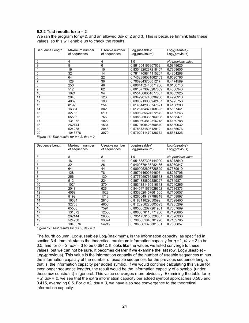
6.2.2 Test results for q = 2We ran the program for q=2, and an allowed dsv of 2 and 3. This is because Immink lists these values, so this will enable us to check the results.

Sequence Length Maximum number of sequences

Useable number of sequences

Log2(useable)/Log2(maximum)

Log2(useable)­Log2(previous)

2 4 4 1.0 No previous value

3 8 6 0.861654166907052 0.5849625 4 16 10 0.8304820237218407 0.7369655 5 32 14 0.7614709844115207 0.4854268 6 64 22 0.7432386031062163 0.6520766 7 128 30 0.700984370801217 0.4474589 8 256 46 0.6904452445071266 0.6166713 9 512 62 0.6615773678207639 0.4306343 10 1024 94 0.6554588851677637 0.6003925 11 2048 126 0.6342981748636288 0.422691012 4069 190 0.6308213006942457 0.592575613 8192 254 0.6145142066747821 0.4188290 14 16384 382 0.6126734877168393 0.5887441 15 32768 510 0.5996235624572572 0.4169246 16 65536 766 0.5988250363703098 0.5868471 17 131072 1022 0.5880693812316248 0.4159788 18 262144 1534 0.5879490426390519 0.5859032 19 524288 2046 0.578873180512912 0.4155076 20 1048576 3070 0.5792011470128772 0.5854325Figure 16: Test results for q = 2, dsv = 2.

Sequence Length Maximum number of sequences

Useable number of sequences

Log2(useable)/Log2(maximum)

Log2(useable)­Log2(previous)

3 8 8 1.0 No previous value

4 16 14 0.9518387305144009 0.8073549 5 32 26 0.9400879436282186 0.8930847 6 64 44 0.9099052697728829 0.7589919 7 128 78 0.897914602694607 0.8259706 8 256 130 0.8777959766285568 0.7369655 9 512 224 0.8674838802286227 0.7849871 10 1024 370 0.8531381460516313 0.7240265 11 2048 626 0.8445471679029652 0.7586373 12 4069 1028 0.8338020457661565 0.7156057 13 8192 1718 0.8266549477798818 0.7408897 14 16384 2810 0.818311029650592 0.7098400 15 32768 4656 0.8123250228605523 0.7285209 16 65536 7594 0.8056652677261931 0.7057689 17 131072 12506 0.8006078118771256 0.7196885 18 262144 20356 0.7951759153320667 0.7028336 19 524288 33374 0.7908651046781228 0.7132705 20 1048576 54242 0.7863561376881381 0.7006857Figure 17: Test results for q = 2, dsv = 3.

The fourth column, Log2(useable)/ Log2(maximum), is the information capacity, as specified in section 3.4. Immink states the theoretical maximum information capacity for q =2, dsv = 2 to be 0.5, and for q = 2, dsv = 3 to be 0.6942. It looks like the values we listed converge to these values, but we can not be sure. It becomes clearer if we examine the last row, Log2(useable) ­Log2(previous). This value is the information capacity of the number of useable sequences minus the information capacity of the number of useable sequences for the previous sequence length, that is, the information capacity per added symbol. If we would continue calculating this value for ever longer sequence lengths, the result would be the information capacity of a symbol (under these dsv constraint) in general. This value converges more obviously. Examining the table for q = 2, dsv = 2, we see that the extra information capacity per added symbol approaches 0.585 and 0.415, averaging 0.5. For q =2, dsv = 3, we have also see convergence to the theoretical information capacity.

25

Indeed, Log2(useable) ­ Log2(previous) converges to the information capacity of a symbol under dsv constraints. We illustrate this alternating convergent behaviour in figure 18 & 19.

Efficiency approximation versus sequence length

0,30,350,40,450,50,550,60,650,70,750,8

3 5 7 9 11 13 15 17 19

Sequence length

Eff

icie

ncy

DSV=2

Figure 18: Alternating convergent behaviour of the efficiency for q=2, dsv=2

Efficiency approximation versus sequence length

0,6

0,65

0,7

0,75

0,8

0,85

0,9

0,95

4 6 8 10 12 14 16 18 20

Sequence length

Eff

icie

ncy

DSV=3

Figure 19: Alternating convergent behaviour of the efficiency for q=2, dsv=3.

Our suspicion now is that the program produces correct results, which we will show in the following section.

26

6.2.3 Integer sequence recognitionUsing the online encyclopedia of integer sequences [16], we found that the useable number of sequences was a known sequence, in particular, for q = 2, dsv = 2, all the values we couldcalculate coincide with sequence A027383 from the encyclopedia. The description of this sequence reads

“Number of balanced strings of length n: let d(S) = #(1)’s in S ­ #(0)’s, then S is balanced

if every substring T has ­2<=d(T)<=2.”

After examination of the description, we conclude that the condition is equal to our definition of Digital Sum Variation. They check whether for every substring, the difference between the number of symbols of one type and symbols of the other type does not exceed certain a certain range (2 in this case). This what ­2<=d(T)<=2 says, you can not have 2 more zeroes than ones in a substring, and not more than 2 more ones than zeroes.If we assign their zero the bipolar ­1 and their one the bipolar 1, we could still use their definition for our definition of the dsv, the number of ­1 symbols should not exceed the number of 1 symbols by more than 2 in any substring, vice versa this should also hold. This way, the variation of the digital sum in a substring can never exceed 2.

We now know that sequence A027383 from [16] is equal to the number of useable binary sequences under dsv constraint D = 2 for a given length SL. This means we can apply the formula that is listed for A027383 to get our results (computationally considerably easier for large sequence lengths). More importantly, we can use the formula to prove that this sequence indeed converges to the theoretical maximum information capacity of 0.5 for q = 2, dsv = 2, which Immink listed.

27

6.2.4 Proof of convergenceIn the last section, we concluded we could use the formula listed for A027383. This formula is

22

))1)(223(223)(2()(

2/

###$$

"nn

na

In this formula, )(na represents the number of sequences as a function of sequence length n.

We will try to prove that )2(

))((

2

2nLog

naLog converges to 0.5.

To this end, we will rewrite ))((2 naLog .

= (2Log 22

))1)(223(223)(2( 2/

###$$ nn

)

Now first rewrite the ­2 term

= (2Log 2/12/2/

222

))1)(223(223)(2( nnnn

$####$$

)

= (2Log )22

))1)(223(223()(2( 12/2/ $##

##$$ nn

n )

= (2Log )2

2

2

))1)(223(223()(2(

22/2/

$#

###$$ nn

n )

= (2Log2

2)1)(223(223()2(

22/2/

$####$$ nnn )

= (2Log 2/2n ) + (2Log 22/2)1)(223(223 $####$$ nn ) ­ (2Log 2)

= $2/n (2Log 22/2)1)(223(223 $####$$ nn ) – 1

Now, dividing by )2(2nLog , (which is simply n ) results in

)/1()/1()2/1( nn $# (2Log 22/2)1)(223(223 $####$$ nn )

For n is even we have

)/1()/1()2/1( nn $# (2Log 22/26 $## n )

For n is odd we have

)/1()/1()2/1( nn $# (2Log 22/224 $## n )

28

In both cases, when n approaches infinity, the terms )/1( n# and )/1( n become zero, and the

argument of the 2Log becomes a constant,6 and 24 for the even and odd case, respectively,

since 22/2 $#n approaches zero for large n . The constant multiplied by the term approaching zero becomes zero, so only the term )2/1( now remains.

So, for n approaching infinity, )2(

))((

2

2nLog

naLog converges to 0.5.

6.3 Optimizing calculationsNow that we showed the correctness of the program results in the previous section, we face a more practical problem, namely that of computational feasibility. The longer the sequences become, the longer it takes for the program to calculate the results. In fact, for a binary alphabet, the amount of work grows with a factor 2 for every added symbol, for a ternary alphabet it grows with a factor 3 for every added symbol. To get a rough idea of the amount of time required, the binary case with a sequence of 10 symbols take about one second, and subsequently doubles for every symbol that is added.We try to counter this by doing sequence concatenation. For example, if we want to know the number of useable sequences of length 10, we generate all the legal sequences of length 5, and we try to concatenate every sequence from this set with every sequence from this set. To find out whether such a concatenation is legal, we define 3 properties for every sequence.These properties are the maximum and minimum digital sum of the sequence and the digital sum at the last position of this sequence. We name these properties DSMax, DSMin and DSLast, respectively. To distinguish between the properties of the first and second sequence (which are to be concatenated), we use the names DSMaxA and DSMaxB for the maximum digital sum of the first and second sequence.

Using these properties, we can formulate the concatenation requirement as

DSMaxA ­ (DSLastA + DSMinB) <= N && DSMinA ­ (DSLastA + DSMaxB) <= N.

Where N is the maximum allowed Digital Sum Variation (inclusive).

We have to use the DSLastA property every time to offset for the possible difference in digital sum value at the border of 2 concatenated sequences. That is, the digital sum might be ­2 at the end of the first sequence, so the maximum and minimal digital sums are downshifted by 2 in the second sequence. We illustrate this in figure 20.

Figure 20, the adjusted dsv values after aligning sequence B with the end of sequence A.

29

When the concatenation requirement is met, we count one legal sequence of length 10. When we do this for all possible combinations, we obtain the number of legal sequences of length 10.Figure 21 is an example of some non­optimized and optimized calculation durations for a range of sequence lengths (q=2, dsv=2).

Sequence length Calculation time (milliseconds) Calculation time (milliseconds, using concatenation)

2 10 10 3 10 10 4 50 10 5 70 20 6 90 50 7 90 40 8 121 30 9 260 60 10 440 50 11 902 60 12 1842 40 13 3735 70 14 8071 70 15 16753 180 16 30062 11117 60112 230 18 128496 220 19 261217 461 20 547509 461 Figure 21: Non­optimized and optimized calculation durations for q=2, dsv=2 using concatenation

As we can see, the gain is very significant, in particular for longer sequences. We see that the optimized calculation time for sequence length 20 (461 milliseconds) is close to the calculation time for sequence length 10 in the non­optimized case. Furthermore, calculation of sequence length 20 for the non­optimized case took about 548 seconds, and such an amount of time is sufficient to calculate sequences of length 40 using concatenation (a simulation result not provided in the table).This leads us to believe that generating half of the sequence length is still the most time consuming process, while calculating whether sequences can be concatenated only requires little time.

The next question that comes naturally is whether we could also do concatenation with more than 2 sequences. For example, to know how many useable sequences of length 30 exist, it might be more efficient to concatenate 3 sequences of length 10 than to concatenate 2 sequences of length 15.In the case of concatenation of 3 or more sequences, we take the approach of first checking concatenation legality of sequence A and B. If it is legal (according to the first criteria), we calculate this concatenated sequence's new DSMax, DSMin and DSLast and use this for checking concatenation legality with sequence C.

We now only need to be able to define a concatenated sequence's new DSMax, DSMin and DSLast in terms of the old DSMax, DSMin and DSLast properties of sequence A and B. We do this using the following rules (in pseudocode).

if (LastA + DSMaxB) > DSMaxA then (LastA + DSMaxB) is the new DSMax.else DSMaxA is the new DSMax.

if (LastA + DSMinB) < DSMinA then (LastA + DSMinB) is the new DSMin.else DSMinA is the new DSMin.

the new Last is LastA + LastB.

30

We name the number of subsequences that a sequence is broken down into the concatenation number. We already implemented the algorithm for a concatenation number of 2.

Implementing this algorithm for the general case of concatenation number = N allows us to measure calculation times given different sequence lengths, dsv values and concatenation numbers. It turned out that the more general algorithm was less efficient than the algorithm we made for a concatenation number of 2, probably as a result from increased memory access. It also appeared that the amount of required memory grows faster, we run out of memory rather soon. We note that using a concatenation number of 3 yields a performance gain for the cases where the dsv is 1, 2, 3 or 4. The tests performed (for sequence lengths 10 through 14 for dsv 1 through 6 and concatenation numbers 2 through 6) did not deliver results that were easy to interpret. No clear relationship was found between the calculation time for the different dsvvalues, concatenation numbers and sequence lengths.

6.4 Efficiency versus dsvThe last paragraph of this chapter will present some results of the calculations by the program for various q values, dsv values and sequence lengths.

Efficiency versus DSV

0,50,550,60,650,70,750,80,850,90,951

2 3 4 5 6 7 8

DSV

Effic

ienc

y

SimulatedLimit

Figure 22 Q=2, dsv=2..8, sequence length = 30. Red is the actual values that Immink listed, blue is the simulated results.

Figure 22 shows 2 plots of the simulated efficiency and the theoretical efficiency limit. The red plot is the theoretical efficiency limit. Given a certain dsv, that is the limit to the efficiency. The blue plot is our approximation of the efficiency using the brute force sequence generation technique described in section 6.2. We see that for increasing dsv values, the difference between the real efficiency and our approximation grows. This can be explained by the fact that our program can only calculate dsv­constrained efficiency for a finite sequence length. If our dsv is 6, we would need at least a sequence length of 6 to start finding illegal sequences, and start approximating the real number of possible sequences given dsv=6. The longer the sequences we are able to calculate, the more illegal sequences for the case dsv=6 we would find, thus increasing our approximation’s precision. If our dsv is 3, we would need at least a sequence length of 3 to start finding illegal sequences, again increasing our precision with increasing sequence lengths. Suppose we can calculate sequences up to length 6. In that case, we have some approximation for dsv=3, but no approximation yet for dsv=6. In general, a larger dsv value requires the program to use a larger sequence length to produce results equally accurate to those for a smaller dsv value.

31

Therefore, a fixed sequence length causes the approximations to be better for smaller dsv values than for large dsv values. In case of dsv=8, the difference between the approximation and actual value is about 3%.We made this plot to get an idea about our programs accuracy given a certain sequence length. This is done because we have no theoretical efficiency limit for other q values, in particular, for q=3, and we want to be able to interpret the results for the ternary case (figure 23) better.

Efficiency versus DSV

0,50,550,60,650,70,750,80,850,90,951

1 2 3 4 5 6 7 8

DSV

Effic

ienc

y

Simulated

Figure 23 Q=3, dsv=1..8, sequence length = 20.

In figure 23, the case of q=3, dsv=1..8, we have no theoretical limit to compare our simulations to. However, according to figure 21 and our previous thoughts, we assume that the real efficiency is slightly smaller, given that there are certain sequences longer than 20 that violate the dsvconstraint. We also note that the results of figure 23 are again more accurate for the lower dsvvalues.

32

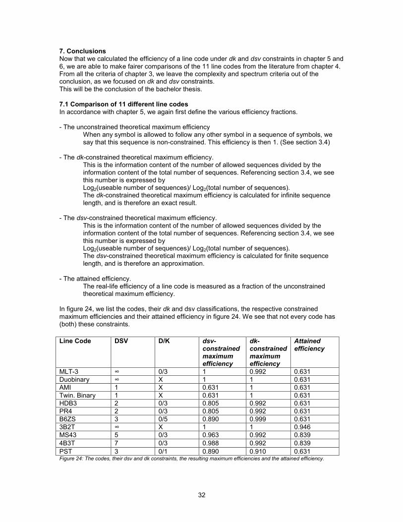
7. ConclusionsNow that we calculated the efficiency of a line code under dk and dsv constraints in chapter 5 and 6, we are able to make fairer comparisons of the 11 line codes from the literature from chapter 4. From all the criteria of chapter 3, we leave the complexity and spectrum criteria out of the conclusion, as we focused on dk and dsv constraints. This will be the conclusion of the bachelor thesis.

7.1 Comparison of 11 different line codesIn accordance with chapter 5, we again first define the various efficiency fractions.

­ The unconstrained theoretical maximum efficiencyWhen any symbol is allowed to follow any other symbol in a sequence of symbols, we say that this sequence is non­constrained. This efficiency is then 1. (See section 3.4)

­ The dk­constrained theoretical maximum efficiency.This is the information content of the number of allowed sequences divided by the information content of the total number of sequences. Referencing section 3.4, we see this number is expressed by Log2(useable number of sequences)/ Log2(total number of sequences). The dk­constrained theoretical maximum efficiency is calculated for infinite sequence length, and is therefore an exact result.

­ The dsv­constrained theoretical maximum efficiency.This is the information content of the number of allowed sequences divided by the information content of the total number of sequences. Referencing section 3.4, we see this number is expressed by Log2(useable number of sequences)/ Log2(total number of sequences). The dsv­constrained theoretical maximum efficiency is calculated for finite sequence length, and is therefore an approximation.

­ The attained efficiency.The real­life efficiency of a line code is measured as a fraction of the unconstrained theoretical maximum efficiency.

In figure 24, we list the codes, their dk and dsv classifications, the respective constrained maximum efficiencies and their attained efficiency in figure 24. We see that not every code has (both) these constraints.

Figure 24: The codes, their dsv and dk constraints, the resulting maximum efficiencies and the attained efficiency.

Line Code DSV D/K dsv-constrained maximum efficiency

dk-constrained maximum efficiency

Attained efficiency

MLT­3 7 0/3 1 0.992 0.631Duobinary 7 X 1 1 0.631AMI 1 X 0.631 1 0.631Twin. Binary 1 X 0.631 1 0.631HDB3 2 0/3 0.805 0.992 0.631PR4 2 0/3 0.805 0.992 0.631B6ZS 3 0/5 0.890 0.999 0.6313B2T 7 X 1 1 0.946MS43 5 0/3 0.963 0.992 0.8394B3T 7 0/3 0.988 0.992 0.839PST 3 0/1 0.890 0.910 0.631

33

7.2 DiscussionOne of the most obvious aspects of figure 25 is that all the codes only have 3 different values for the attained efficiency, that is, 0.631 (8 codes), 0.839(2 codes) and 0.946 (1 code). The dk­constraints (or, more specifically, k­constraints, since d is always zero in our case), have only minor impact on the efficiency. The dsv­constraints have a more significant impact. Indeed, for a dsv­constraint of 1, only two different symbols are allowed after any symbol, yielding an efficiency equal to that of a binary code. For higher dsv values, we see maximum possible efficiency is much higher, and quickly approaches values greater than 95% (for a dsv of 5).

We have a few codes that are equally constrained.PR4 and HDB3 both have a dsv constraint of 3 and a maximum runlength (k constraint) of 3, and have the same efficiency. All else equal, one would choose the code with the simplest implementation.Another illustrating example is the 3B2T code and the Duobinary code. They are both non­constrained, so have the same theoretical maximum efficiency (which is 1). 3B2T utilizes 95% of its theoretical maximum efficiency, while Duobinary is only as efficient as a binary code (63%). This could lead one to say that 3B2T is a lot better, but keep in mind that the complexity for Duobinary is very low (it is a linear code) while 3B2T uses tables (higher complexity). There lies the trade­off. Also interesting are AMI and Twinned Binary, which both exactly attain their theoretical maximum efficiency.

We could also look at the efficiency a code attains, and compare the constraints. MS43 and 4B3T both attain 84% efficiency. Their dk­constraint is equal, but the dsv constraint for MS43 is better (5) than that for 4B3T (7). This is also explicitly noted by the author of [4].

One might be tempted to multiply the dk­constrained and dsv­constrained efficiency fractions and consider it the maximum theoretical efficiency attained for a combination of dk and dsv constraints, but we note that these 2 constraints are not mutually independent. For example, in the case of dk constraints 0,2 and dsv = 2, the ternary sequence of sequence length 3: + + +, is excluded from the useable sequences by both the dk and dsv constraint.We found one table in reference [18] listing the efficiency of a code under combined dk­dsv constraints. Specifically, they list the capacity of a binary code for a dsv­constraint 5, and dkconstraints of 0,1; 0,2; 0,3 and 0,4. However, consulting their references did not provide a clear source for the relationship between the efficiency and combined dk­dsv constraints.

In general, we note that choosing a line code is usually the result of engineering requirements. We have a specific medium, a specified clock precision, etcetera. The dk and dsv constraints following from these requirements yield an upper bound of the efficiency to which the medium can be utilized. When choosing (or developing) a line code, we can always check whether it approaches the constrained theoretical maximum efficiency. In theory, there is always a code that does attain this efficiency [18]. In real life, there is the practical concern of coder/decoder complexity, which causes a limited efficiency. This is the tradeoff. The authors of [18] have done research that includes a formal measure for code complexity as a factor for evaluating line codes.

34

8. References

1 F.T. Andrews, "Bipolar Pulse Transmission and Regeneration" U.S. Patent 2996578 Aug. 15, 1961.

2 “Transmission Systems for Communications”, Bell Telephone Laboratories, 19713 J.M. Sipress, "A new class of selected Ternary Pulse Transmission Plans for Digital

Transmission Lines", IEEE transactions on Communication Technology, COM­13, 1965.4 A. Croisier, “Introduction to pseudoternary Transmission Codes”, IBM Journal of

Research and Development, July 1970.5 W. Stallings, "ISDN and Broadband ISDN with Frame Relay and ATM", ISBN 0­13­

973744­86 M. R. Aaron, “PCM Transmission in the Exchange Plant,” Bell System Technical Journal,

Vol. 41, pp. 99­141 (January 1962).7 Intersil, description of “The HC­5560 Digital Line Transcoder”

http://www.intersil.com/data/an/an573.pdf 1997.8 P.A. Franaszek, “Sequence State Coding for Digital Transmission”, Bell System

Technical Journal 47, pp 143, 1968.9 Réne H.M. Kohlman, “The physical layer of the Twentenet local area network”, Doctoral

assignment University Twente, Reportnumber 1251­82­12, October 1982.10 K. A. Schouhamer Immink, “Coding techniques for Digital Recorders” Prentice Hall, 1991

ISBN 0­13­140047­9.11 A.J. van Wijngaarden, K.A. Schouhamer Immink, “On the selection of guided scrambling

sequences that provide guaranteed maximum run­length constraints” http://www.exp­math.uni­essen.de/~immink/pdf/gscc_not.pdf

12 Mazzola, et al. United States Patent 5,280,500 January 18, 1994.13 P.T. de Boer, sheets for the course “Telematica Netwerken 2004”, University Twente. 14 D.T. Tang and L.R. Bahl, “Block codes for a class of constrained noiseless channels”,

Information and Control, issue 17, page 436­461, 1970.15 E.R. Kretzmer, “Generalization of a Technique for Binary Data Communication”, IEEE

Transactions on Communication Technology, page 67­68, February 1966.16 N. J. A. Sloane, (2006), The On­Line Encyclopedia of Integer Sequences,

www.research.att.com/~njas/sequences/17 E. Laroche, June 2002

http://www.lrdev.com/lr/java/BigRational.html18 A.X. Widmer, P.A. Franaszek, “A DC­balanced, partitioned­block, 8B/10B transmission

code”, IBM Journal of research and development, volume 27, no. 5, September 198319 Ta­Mu Chien, “Upper bound on the efficiency of DC­constrained codes”, Bell system

technical journal, volume 49, pp 2267­2287, 1970.