
Information Hiding and Covert Communication Hamming codes generate embedding codes all distinct...
55
Information Hiding and Covert Communication Andrew Ker adk @ comlab.ox.ac.uk Royal Society University Research Fellow Oxford University Computing Laboratory Foundations of Security Analysis and Design Bertinoro, Italy, 25-26 August 2008
Transcript of Information Hiding and Covert Communication Hamming codes generate embedding codes all distinct...

Information Hiding
and Covert Communication
Andrew [email protected]
Royal Society University Research Fellow
Oxford University Computing Laboratory
Foundations of Security Analysis and Design
Bertinoro, Italy, 25-26 August 2008

Part 3: More Efficient Steganography
• Abstraction of the embedding problem, simple example of efficiency
• Embedding codes
– Syndrome codes: the Hamming code family
• Embedding efficiency bound
• More embedding codes
– Golay code
– The ZZW construction
• Asymptotics
Information Hiding
and Covert Communication

Abstraction- separate the embedding operation from the details of what payload is
embedded where.
Say that
• the cover consists of a number of locations,
• each location contains one q-ary symbol,
• an embedding change alters the symbol at one location.
Embedding operations might be: replacement of LSB of pixel, adjustment of
LSB of quantized coefficient, adjustment of remainder (mod q) …
Aim: maximize the amount of information transmitted, while minimizing
the number of embedding changes.
(Implicitly: all embedding changes are equally risky.)
We stick to binary symbols,

Embedding efficiency
Regardless of payload size, on average each bit of payload requires 0.5
embedding changes.
We say that the embedding efficiency bits per change.
0 1 0 0 1 1 0 1 1 0 0 0 0 1 1 0 1 1 0 …
0 0 1 1 0 1 1 1 1 0 1 1 0 0 1 1 0 1 1 …
0 0 1 1 0 1 1 1 1 0 1 1 0 0 1 1 0 1 1 …
Cover:
Payload:
Stego:

Example of efficient embedding
0 0 1 1 0 1 1 1 1 0 1 1 …
0 0 0 1 1 1or0 0
0 0 1 1 1 0or0 1
0 1 0 1 0 1or1 0
1 0 0 0 1 1or1 1
Cover:
Payload:
Take cover in groups of 3, payload in groups of 2.
Embed a payload group in each cover group using the encoding:
0 0 0 0 1 1 0 0 1 1 0 0 0 1 0 0 1 1 0 …Stego:
0 1 0 0 1 1 0 1 1 0 0 0 0 1 1 0 1 1 0 …

Example of efficient embedding
0 0 1 1 0 1 1 1 1 0 1 1 …
0 0 0 0 1 1 0 0 1 1 0 0 0 1 0 0 1 1 0 …
Cover:
Payload:
Stego:
Payload rate
Embedding changes:
with probability
with probability
Embedding efficiency bits per change.
0 0 0 1 1 1or0 0
0 0 1 1 1 0or0 1
0 1 0 1 0 1or1 0
1 0 0 0 1 1or1 1
0 1 0 0 1 1 0 1 1 0 0 0 0 1 1 0 1 1 0 …

Embedding codesA binary embedding code is:
• a partition of into subsets
• an embedding map with
The average embedding distance is
We say that the code is
It achieves a payload rate of with embedding efficiency
e.g. is with
000 001
100 101
010 011
110 111

Embedding codes
e.g.
is with
01010011 110010100110 1001
1111
10110111 11101101
0000
00100001 10000100

Syndrome coding• A linear code is a k-dimensional subspace of
• Its parity check matrix is a matrix s.t. iff
• For each s in the coset leader for s is a vector
with least weight (number of 1s) such that
Matrix Embedding Theorem
Every linear code generates a embedding code by the
following construction:
Then is the average weight of all coset leaders.
J. Fridrich & D. Soukal. Matrix Embedding for Large Payloads. IEEE Trans. Information Forensics and Security 1(3), 2006.
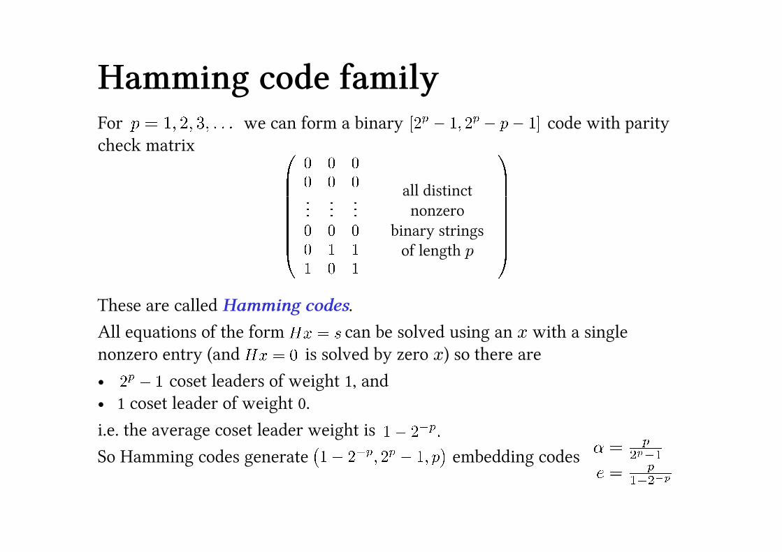
Hamming code familyFor we can form a binary code with parity
check matrix
These are called Hamming codes.
All equations of the form can be solved using an x with a single
nonzero entry (and is solved by zero x) so there are
• coset leaders of weight 1, and
• 1 coset leader of weight 0.
i.e. the average coset leader weight is
So Hamming codes generate embedding codes
all distinct
nonzero
binary strings
of length p

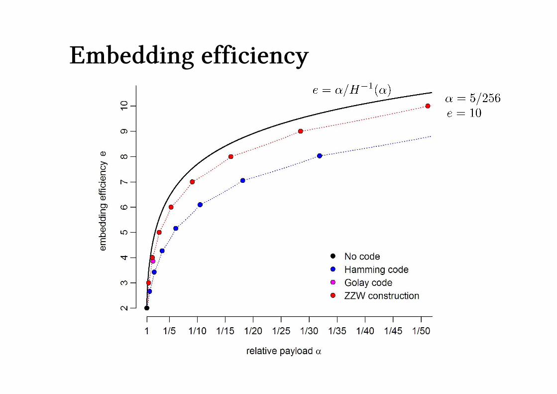
Embedding efficiency

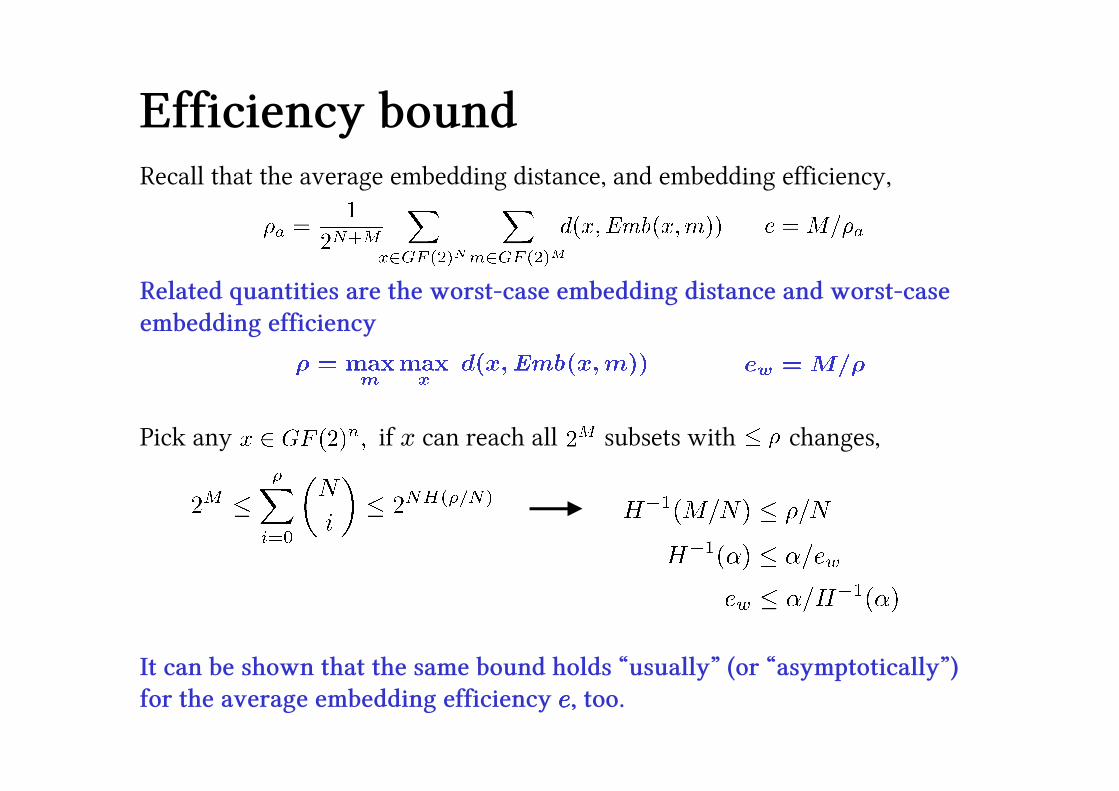
Efficiency boundRecall that the average embedding distance, and embedding efficiency,
Related quantities are the worst-case embedding distance and worst-case
embedding efficiency
Pick any if x can reach all subsets with changes,

Binary entropy function
Efficiency boundRecall that the average embedding distance, and embedding efficiency,
Related quantities are the worst-case embedding distance and worst-case
embedding efficiency
Pick any if x can reach all subsets with changes,
It can be shown that the same bound holds “usually” (or “asymptotically”)
for the average embedding efficiency eeee, too.

Embedding efficiency
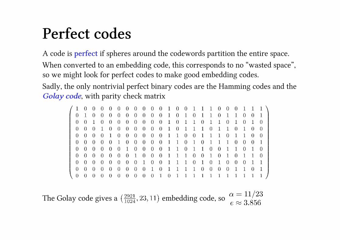
Perfect codesA code is perfect if spheres around the codewords partition the entire space.
When converted to an embedding code, this corresponds to no “wasted space”,
so we might look for perfect codes to make good embedding codes.
Sadly, the only nontrivial perfect binary codes are the Hamming codes and the
Golay code, with parity check matrix
The Golay code gives a embedding code, so

Embedding efficiency

The ZZW constructionFix positive integer Split cover into groups of size
For each group, suppose that the cover bits are Compute their XOR
• If this matches next payload bit, change nothing.
(0 embedding changes, 1 bit of information transmitted)
• If the XOR does not match the payload bit, change one of the locations
Communicate additional bits by the choice of which to change.
(1 embedding change, bits of information transmitted)
W. Zhang, X. Zhang, & S. Wang. Maximizing Steganographic Embedding Efficiency by Combining Hamming Codes and Wet Paper Codes. In Proc. 10th Information Hiding Workshop, Springer LNCS, 2008.

The ZZW constructionFix positive integer Split cover into groups of size
For each group, suppose that the cover bits are Compute their XOR
• If this matches next payload bit, change nothing.
(0 embedding changes, 1 bit of information transmitted)
• If the XOR does not match the payload bit, change one of the locations
Communicate additional bits by the choice of which to change.
(1 embedding change, bits of information transmitted)
Clever bit: how does the recipient know
which groups had a change? - Wet Paper codes
which of was changed? - Hamming codes
On average, we have a embedding code.
Embedding efficiency
Embedding efficiency

Embedding 5120 bits in 262144 locations by
simple replacement: 2560 changes.

Embedding 5120 bits in 262144 locations by
ZZW code: 512 changes.

Asymptotic relationshipSince we can deduce an asymptotic relationship between
cover size n, total number of embedding changes c, and total embedded
payload p:
(as )
(as )

Part 4: Steganographic Capacity
• Concept of capacity
• Capacity of perfect steganography
– The amount of information you can hide is proportional to the cover size
• Capacity of batch steganography
– … proportional to the square root of the number of covers
• Capacity of Markov covers
– … proportional to
• Reconciliation, experimental results
Information Hiding
and Covert Communication

Detector performance
… the more information you hide, the greater the risk of discovery.

Capacity- the more information you hide, the greater the risk of discovery.
Fix an embedding method & cover source.
• Given a limit on “risk”, what is the largest payload which can safely be
embedded?
• How does this safe maximum payload depend on the size of the cover?

Perfect steganography- steganography with no risk.
For there to be no risk, the cover objects and the stego objects must have
exactly the same statistical properties.
Theorem
Randomly modulated codes constructed from codes with “order-1 security”
produce perfect steganography.
The amount of information which can be hidden using these randomly
modulated codes depends on the cover source, but is guaranteed to be ,
where n is the number of symbols transmitted.
Y. Wang & P. Moulin. Perfectly Secure Steganography: Capacity, Error Exponents, and Code Constructions. IEEE Trans. Information Theory 54(6), 2008.

Moral
Given perfect knowledge of the cover source, the amount of information you
can hide is proportional to the cover size.
but… constructing the perfect embedding code requires complete and
perfect knowledge of the cover source.
Nobody has perfect knowledge of their cover source!
“Model-based steganography” by Sallee, 2003
… broken by Fridrich in 2004
“Stochastic QIM” by Moulin & Briassouli, 2004
(described as “robust” and “undetectable”)
… broken by Wang & Moulin in 2006

Capacity- the more information you hide, the greater the risk of discovery.
Fix an embedding method & cover source.
• Given a limit on “risk”, what is the largest payload which can safely be
embedded?
• How does this safe maximum payload depend on the size of the cover?
Ross Anderson in the 1st Information Hiding Workshop (1996):
“…the more covertext we give the warden [detector], the better he will be able to estimate its statistics, and so the smaller the rate at which Alice will be able to tweak bits safely. The rate might even tend to zero...”

Capacity- the more information you hide, the greater the risk of discovery.
Fix an embedding method.
• Given a limit on “risk”, what is the largest payload which can safely be
embedded?
• How does this safe maximum payload depend on the size of the cover?
… implicitly assumes that the Warden seeks a binary decision. “Safe” can be
defined in terms of false positive rate α and false negative rate β:
embedding a certain payload is “safe” if any steganalysis detector must
have more than a certain false positive and false negative rate.

Information theoretic bounds- bounds detection performance using Kullback-Leibler divergence.
If X has density function f, and Y has density function g, then the KL
divergence from X to Y is
Information Processing Theorem:
Therefore, if trying to separate an instance of X from one of Y, the false
positive (Y) rate α and false negative (X) rate β must satisfy
C. Cachin. An Information-Theoretic Model for Steganography. Information and Computation 192(1), 2004.

Information theoretic bounds- bounds detection performance using Kullback-Leibler divergence.
If X has density function f, and Y has density function g, then the KL
divergence from X to Y is
Information Processing Theorem:
Therefore, if trying to separate an instance of X from one of Y, the false
positive (Y) rate α and false negative (X) rate β must satisfy
To apply this, we need to know
We have already seen that statistical models for covers are inaccurate.

Batch steganography- instead of performing steganography and steganalysis in isolated
objects, consider a large number of covers.
A. Ker. Batch Steganography & Pooled Steganalysis. In Proc. 8th Information Hiding Workshop, Springer LNCS, 2006.

cover
payload:
m bits em
bed
din
g
Warden
Alice
extrac
tion
secret key
Bob?

nco
ver
s
payload:
m bits em
bed
din
g
embed λ1 bits
Warden…
…
…
embed λ2 bits
embed λn bits
Alice
extrac
tion
secret key
Bob
……
any ?
……

nco
ver
s
payload:
m bits em
bed
din
g
embed λ1 bits
Warden…
…
…
embed λ2 bits
embed λn bits
Alice
extrac
tion
secret key
Bob
……
any ?
……
has p.d.f.
Choice of λi s.t.
is Alice’s embedding strategy
Converting X into a
decision is Warden’s
pooling strategy

Batch steganographic capacityA tractable and interesting capacity question:
How does maximum secure capacity depend on the number of covers n?
It turns out that the order of growth is independent of all the other capacity
factors.
A. Ker. A Capacity Result for Batch Steganography. IEEE Signal Processing Letters 14(8), 2007.
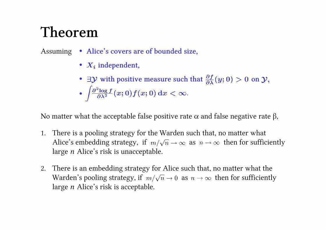
TheoremAssuming � Alice’s covers are of bounded size,
� independent,
� with positive measure such that on
�
No matter what the acceptable false positive rate α and false negative rate β,
1. There is a pooling strategy for the Warden such that, no matter what
Alice’s embedding strategy, if as then for sufficiently
large n Alice’s risk is unacceptable.
2. There is an embedding strategy for Alice such that, no matter what the
Warden’s pooling strategy, if as then for sufficiently
large n Alice’s risk is acceptable.

Proof sketch1. There is a pooling strategy for the Warden such that… if
then… Alice [will be eventually caught].
The pooling strategy is:
payload detected if is greater than a critical threshold
By the Berry-Esséen Theorem (& independence):
Detector performance tends to perfect, as n →→→→∞∞∞∞
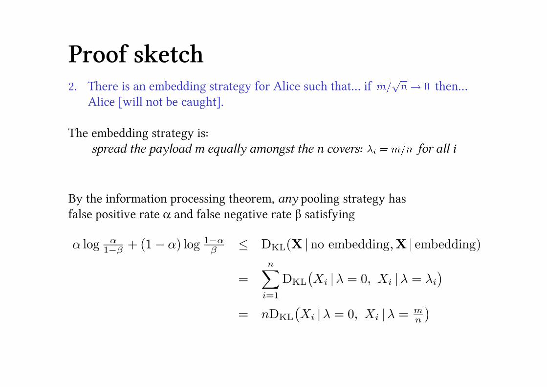
Proof sketch2. There is an embedding strategy for Alice such that… if then…
Alice [will not be caught].
The embedding strategy is:
spread the payload m equally amongst the n covers: for all i
By the information processing theorem, any pooling strategy has
false positive rate α and false negative rate β satisfying

Proof sketch
Detector performance tends to random, as n →→→→∞∞∞∞

TheoremAssuming � Alice’s covers are of bounded size,
� independent,
� with positive measure such that on
�
No matter what the acceptable false positive rate α and false negative rate β,
1. There is a pooling strategy for the Warden such that, no matter what
Alice’s embedding strategy, if as then for sufficiently
large n Alice’s risk is unacceptable.
2. There is an embedding strategy for Alice such that, no matter what the
Warden’s pooling strategy, if as then for sufficiently
large n Alice’s risk is acceptable.
Common senseEmbedding
makes something
more (or less)
likely
Finite Fisher Information

TheoremAssuming � Alice’s covers are of bounded size,
� independent,
� with positive measure such that on
�
No matter what the acceptable false positive rate α and false negative rate β,
1. There is a pooling strategy for the Warden such that, no matter what
Alice’s embedding strategy, if as then for sufficiently
large n Alice’s risk is unacceptable.
2. There is an embedding strategy for Alice such that, no matter what the
Warden’s pooling strategy, if as then for sufficiently
large n Alice’s risk is acceptable.
3. What if ?
Common senseEmbedding
makes something
more (or less)
likely
Finite Fisher Information
Moral
Given some conditions on the covers, the amount of information you can hide
is proportional to the square root of the number of covers.
but… what about individual covers?

Steganography in Markov chains- turn to single cover objects, with a very general model.
• Model the cover source as a Markov chain, a memoryless finite state
machine moving at random from state to state.
The sequence of states is denoted
The states could represent the pixels of a cover image, or the quantized
DCT coefficients, or groups of pixels, etc.
• We model the embedding process as random substitution of states described
by a matrix : if the stego object is and the embedding change rate is
T. Filler, A. Ker, & J. Fridrich. The Square Root Law of Steganographic Capacity for MarkovCovers. To appear in Proc. Electronic Imaging 2009, SPIE.

Steganography in Markov chains- turn to single cover objects, with a very general model.
• Model the cover source as a Markov chain, a memoryless finite state
machine moving at random from state to state.
The sequence of states is denoted
The states could represent the pixels of a cover image, or the quantized
DCT coefficients, or groups of pixels, etc.
• We model the embedding process as random substitution of states described
by a matrix : if the stego object is and the embedding change rate is
(We must have for all x. If also for all y, the embedding
is called doubly stochastic.)

TheoremAssuming � Markov chain is irreducible,
� Embedding is independent of cover,
� Embedding is doubly stochastic,
� There is some sequence such that
No matter what the acceptable false positive rate α and false negative rate β,
1. There exists a detector such that, if the embedding rate γ satisfies
as then for sufficiently large n Alice’s risk is unacceptable.
2. For any detector, if the number of embedding rate γ satisfies
as then for sufficiently large n Alice’s risk is acceptable.
Common sense
Embedding
makes something
more (or less)
likely
Ensures convergence to
equilibrium
# embedding changes

Moral
Given a Markov cover source and random embedding satisfying some weak
conditions, the number of embedding changes you can make is proportional to
the square root of the cover size.
Recall, with asymptotically efficient embedding codes, the payload size p and
the number of embedding changes c can satisfy
Then implies
ReconciliationMoulin’s theorem says:
Steganographic capacity is linear,
if Alice knows her cover source perfectly.
Batch steganographic theorem says:
Steganographic capacity is a square root law,
if (roughly) Alice’s embedding is imperfect (and non-adaptive).
Markov chain capacity theorem says:
Steganographic capacity measured in embedding changes is a square root law,
if (roughly) Alice’s embedding is imperfect (and non-adaptive).

Experimental resultsWe would like to test some contemporary steganography and steganalysis
methods, to see if a square root law is observed.
Idea:
• Create image sets of different sizes.
• Embed lots of different-size payloads in each set, perform steganalysis.
• Look for the relationship between cover and payload size and detectability.
It is difficult to make image sets of different sizes which do not also have
different characteristics: noise, density, etc.
The best we can do is crop down large images to smaller ones, choosing the
crop region to preserve local variance or a similar noise statistic.
A. Ker, T. Pevný, J. Kodovský, & J. Fridrich. The Square Root Law of Steganographic Capacity. To appear in Proc. Multimedia & Security Workshop 2008, ACM.

Experimental resultsLSB replacement steganography & Couples steganalysis

Experimental resultsF5 steganography & “Merged features” SVM steganalysis

Conclusions• The complete square root law for capacity will be a suite of theorems,
proving the result under different circumstances.
We already know some conditions under which it holds, and it appears
to hold in practice too.
• Although many authors describe steganography and steganalysis payloads
in terms of “bits per pixel” or “bits per nonzero DCT coefficient”, it is more
accurate to think in terms of “bits per square root pixel,” etc.
• A big outstanding question: what is the multiplicative constant in the square
root law?
It will depend on the cover source and the embedding method:
– could use this to compare the security of different embedders,
– could also compare the security of different cover sources.