Temporal trends in shade sensitive

epiphytic cryptogams residing on old trees

Master thesis in Biology

Biodiversity, Evolution and Ecology

Anette Gundersen

August 2013

Abstract

Question: How does abandoned management affect species assemblages of shade sensitive

bryophytes and lichens residing on old trees in traditionally light- open environments?

Method: I examined compositional change over 20 years in the epiphytic vegetation of old

pollarded trees of Fraxinus excelsior in a cultural landscape of western Norway through re-

sampling. The nature of changes in the epiphytic composition in relation to environment was

identified through 1) Quantifying temporal turnover in species compositions along DCA axes;

2) Calculation of relative changes in Ellenberg indicator values for gradients of light and

moisture through a weighted average technique and 3) Testing the effect of aspect, stem

inclination/ height and the historical management regime on the rate of temporal turnover.

This was done by mixed effect models with forward selection.

Results: Species composition of the epiphytic vegetation has changed significantly during the

last 20 years. Species with lower indicator values for light (shade tolerant species) and higher

indicator values for moisture (draught sensitive species) increased in relative abundance. An

environmental trend towards more shady and moist conditions was detected. Among other

shade sensitive species, shade and draught sensitive cyanolichens are negatively affected,

whereas the shade and draught tolerant chlorolichens and liverworts residing throughout the

stem within sheltered local environments, like Lepraria spp, Phlyctis argena and Metzgeria

conjugata gain advantage.

Synthesis: The results imply a negative impact of abandoned management on temporal trends

in assemblages of shade sensitive epiphyte bryophytes and lichens. The results demonstrated

that the combination of approaches employed is operational and conceptually relevant for

detecting temporal trends in cryptogam epiphytic communities in relation to environment at

the scale of the landscape.

Acknowledgements

My deepest gratitude goes to my main supervisor John- Arvid Grytnes for his creative

suggestions, excellent supervising, critical comments and positive, encouraging attitude. I am

also grateful to Tor Tønsberg and Hans Blom for valuable help in field, identification of

species and writing corrections.

A special thanks to Astrid Botnen and Bjørn Moe who made this study possible through their

original study in 1997. They were also of great help in the search for the original data and for

identification of the pollards.

Help from employees at Havrå was crucial for detection of the pollards and time since last

pollarding: Thank you Kjetil Monstad, Marit Adelsten Jensen and Tove Mostrøm!

Thanks Olav for your skills in editing and for taking good care of Ella and Ingvill. Without

the impressive support from both pairs of grandparents I would not have been able to achieve

this work: I am so grateful to you all! Finally thanks to Ella and Ingvill for cheerful and

supportive company and patience with a busy, boring mother.

Anette Gundersen

August 2013

Contents

Chapter 1. Introduction ........................................................................................................................... 1

Chapter 2. Materials and methods.......................................................................................................... 3

Investigation area ................................................................................................................................ 3

Sampling .............................................................................................................................................. 4

Detrended Correspondence Analysis (DCA) ........................................................................................ 7

Strength of relation between variables ............................................................................................... 8

Temporal turnover .............................................................................................................................. 8

DCA axes .......................................................................................................................................... 8

Light and moisture gradients .......................................................................................................... 8

Direction of temporal turnover ........................................................................................................... 9

Rate of temporal turnover .................................................................................................................... 10

Chapter 3. Results.................................................................................................................................. 12

DCA .................................................................................................................................................... 12

Ecological interpretation of DCA axes ............................................................................................... 12

Temporal turnover in species composition ....................................................................................... 15

Importance of Aspect, Height and Management to temporal turnover rate ................................... 16

Chapter 4. Discussion ............................................................................................................................ 23

Main results ....................................................................................................................................... 23

Interpretation of DCA axes ................................................................................................................ 24

DCA axis 1 ...................................................................................................................................... 24

DCA axis 2 ...................................................................................................................................... 24

DCA axis 3 ...................................................................................................................................... 25

DCA axis 4 ...................................................................................................................................... 26

Direction of temporal turnover. ........................................................................................................ 26

Temporal trends revealed along gradients in light and moisture ................................................. 26

Temporal trends revealed along DCA axis 2 .................................................................................. 27

Temporal trends revealed along DCA axis 4 .................................................................................. 27

Variation in temporal turnover rates along DCA axis 4 ..................................................................... 28

Variation in temporal turnover rates along DCA axis 2 ..................................................................... 28

Uncertainties ..................................................................................................................................... 29

Management implications ................................................................................................................. 30

Chapter 5. Concluding remarks ............................................................................................................. 31

References ............................................................................................................................................. 33

Figures ................................................................................................................................................... 39

Tables .................................................................................................................................................... 39

Appendix 1. Species list with Ellenberg indicator values ...................................................................... 40

Appendix 2. UTM positions ................................................................................................................... 44

Appendix 3. Ecological interpretation of DCA axes. .............................................................................. 45

DCA Axis 1. ......................................................................................................................................... 45

DCA Axis 2 .......................................................................................................................................... 46

DCA Axis 3 .......................................................................................................................................... 48

DCA Axis 4 .......................................................................................................................................... 51

Appendix 4. Importance of Height, Aspect and Management .............................................................. 52

1

Chapter 1. Introduction

The additive effects of agricultural change and silvicultural practices is expected to reduce the

future viability of shade sensitive old- forest epiphytes throughout Europe (Ellis 2012;

Johansson et al. 2013). Old pollarded trees are traditionally managed trees historically

residing in different kinds of light- open wooded grasslands. High variation in ecological

niches throughout the pollarded trunk provides habitats for many groups of organisms. Old

pollards in open meadows are as such important to the survival of old growth, rare or

endangered epiphytes adapted to light- open environments, like Agonimia Allobata, Lobaria

scrobiculata and Thelopsis rubella (Rose 1992; Nilsson et al. 1994; Tønsberg et al. 1996,

Gauslaa & Ohlson 1997; Moe & Botnen 1997, 2000; Bendiksen et al. 2008; Timdal et al.

2010).

Ceased pollarding and development of secondary woodland, followed by reduction in

openness represent a main threat to many red- listed epiphytes (Jüriado et al. 2003; Johanson

2006). The degree of current openness is however conditioned by habitat history, and change

in openness alters habitat conditions in terms of moisture, temperature and ventilation (Ranius

et al. 2008). Humidity and shading is important to epiphytic composition (Leppik et al. 2011),

and lichen assemblages are supposed to be more limited by light and less sensitive to

desiccation than bryophytes (Kiraly et al. 2013). Low light availability limits lichen growth,

but excessive light can however cause photoinhibition and quicken the dehydration of thalli

(Green et al. 2008, Palmqvist et al. 2008). Studies on the photosynthetic activity of lichens

claim that chlorolichens, as many other poikilohydric organisms like bryophytes, need

nothing but humidity for initiation of their active period, as compared to cyanolichens who

need liquid water (Lange et al. 1986; Büdel et al. 2013).

Several recent studies have addressed the impact of overgrowth to epiphytic diversity in

European wooded grasslands (Leppik & Jüriado 2008; Juriado et al. 2009; Jönsson et al.

2011; Leppik et al. 2011; Jüriado et al. 2012; Johansson 2012; Marmor et al. 2012; Johanson

et al. 2013; Ódor et al. 2013). In studies like these concerned with factors structuring

epiphytic richness and composition, most often the spatial component of change in

community structure from one sampling unit to another (turnover) and the levels of tree and

stand are addressed (cf. Johansson 2006; Ellis 2012). To my knowledge, no study has ever

measured temporal turnover in epiphytic communities of bryophytes and lichens at the fine

2

scale and along environmental gradients, what might provide insights into the specific nature

of epiphytic community development in relation to environment.

Old pollarded trees of Fraxinus excelsior and Ulmus glabra reside in the heterogeneous

landscape of the cultural environment of Havrå. Moe & Botnen (1997) found that the species

compositions of epiphytic bryophytes and lichens residing on the pollarded ash trees varied

among trunks within local stands of variable openness across the landscape of Havrå. The

high age (several hundred years) of the pollarded ash trees at Havrå, followed by slow vertical

growth, provides high similarities in bark structure and consequently pH throughout the stem

(even though fine- scale variations in bark chemistry may occur among discrete areas of the

bole and along the height of the stem due to differences in stem- flow (Marmor et al. 2010)).

High lateral and vertical heterogeneity in environments of light and moisture throughout the

pollarded bole corresponds to a high within- tree variability in epiphytic composition along

gradients of height/ stem inclination and aspect (Moe & Botnen 1997, 2000; Nordbakken &

Austad 2010).

The combination of relatively high within- bole similarity in bark pH and high heterogeneity

in environments of light and moisture throughout the pollarded stems provide favourable

conditions for quantification of temporal turnover at the fine scale in relation to availability of

light and moisture. Turnover requires one to define a specific gradient of interest with

directionality (Andersson et al. 2011). In this study the community data on relative species

abundances and associated environmental data of Moe & Botnen (1997) is re- sampled with

the aim of answering the following questions: 1) Has there been any directional change in the

species composition of the epiphytic communities on the pollarded trees at Havrå, with

emphasis on the role of light and moisture availability? 2) Does the observed changes vary

with the historical management regime of the pollards and surrounding meadows? 3) Is aspect

and height important to within- tree variability in the observed changes? This approach may

provide insight into the role of abandoned management to the future viability of assemblages

of shade sensitive bryophytes and lichens residing on old trees in traditionally light- open

landscapes.

3

Chapter 2. Materials and methods

Investigation area

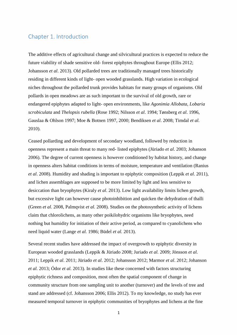
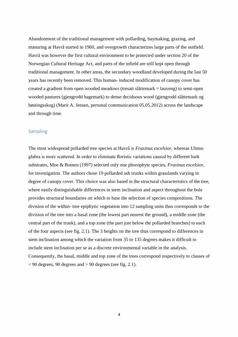
The fieldwork of this study was performed at the southern side of the island Osterøy in

western Norway, in the cultural landscape of the farm Havrå (Figure 1). Situated

approximately 35 km from the coastline of Hordaland County, the area belongs to the

boreonemoral vegetation zone (BN), within the markedly oceanic vegetation section, sub

section humid (03h) (Moen et al. 1999). Mean temperature for the warmest month of July is

14 degrees, 0 degrees for the coldest month of January, and mean annual precipitation is

approximately 2500 mm (Jordal & Gaarder 2009). A favourable local climate provides longer

growth season as compared to other areas of the region (Austad & Skogen 1990). The

bedrock of the area consists of a mica-schistzone in the major Bergen arc system and the soil

in the area is fairly nutrient rich (Austad & Skogen 1988). The 31 farm buildings at Havrå,

and the surrounding fields within which the pollards of investigation reside, are situated

within an area of approximately 0.2 km2 rising from sea- level to 220 m. The steep south-

facing slope of the area provide maximum insolation. During winter however, insolation is

reduced due to shadow from the high mountains on the opposite side of Sørfjorden.

Figure 1: Map indicating the study area Havrå with a yellow arrow. The map is taken from norgeskart.no/ Norwegian national mapping authority.

4

Abandonment of the traditional management with pollarding, haymaking, grazing, and

manuring at Havrå started in 1960, and overgrowth characterizes large parts of the outfield.

Havrå was however the first cultural environment to be protected under section 20 of the

Norwegian Cultural Heritage Act, and parts of the infield are still kept open through

traditional management. In other areas, the secondary woodland developed during the last 50

years has recently been removed. This human- induced modification of canopy cover has

created a gradient from open wooded meadows (tresatt slåttemark = lauveng) to semi-open

wooded pastures (gjengrodd hagemark) to dense deciduous wood (gjengrodd slåttemark og

høstingsskog) (Marit A. Jensen, personal communication 05.05.2012) across the landscape

and through time.

Sampling

The most widespread pollarded tree species at Havrå is Fraxinus excelsior, whereas Ulmus

glabra is more scattered. In order to eliminate floristic variations caused by different bark

substrates, Moe & Botnen (1997) selected only one phorophyte species, Fraxinus excelsior,

for investigation. The authors chose 19 pollarded ash trunks within grasslands varying in

degree of canopy cover. This choice was also based in the structural characteristics of the tree,

where easily distinguishable differences in stem inclination and aspect throughout the bole

provides structural boundaries on which to base the selection of species compositions. The

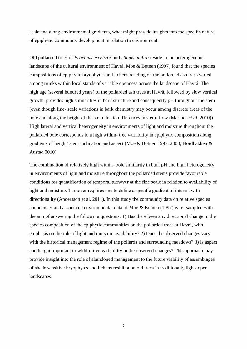
division of the within- tree epiphytic vegetation into 12 sampling units thus corresponds to the

division of the tree into a basal zone (the lowest part nearest the ground), a middle zone (the

central part of the trunk), and a top zone (the part just below the pollarded branches) to each

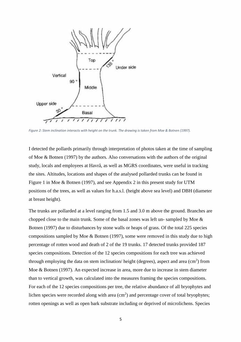
of the four aspects (see fig. 2.1). The 3 heights on the tree thus correspond to differences in

stem inclination among which the variation from 35 to 135 degrees makes it difficult to

include stem inclination per se as a discrete environmental variable in the analysis.

Consequently, the basal, middle and top zone of the trees correspond respectively to classes of

< 90 degrees, 90 degrees and > 90 degrees (see fig. 2.1).

5

Figure 2: Stem inclination interacts with height on the trunk. The drawing is taken from Moe & Botnen (1997).

I detected the pollards primarily through interpretation of photos taken at the time of sampling

of Moe & Botnen (1997) by the authors. Also conversations with the authors of the original

study, locals and employees at Havrå, as well as MGRS coordinates, were useful in tracking

the sites. Altitudes, locations and shapes of the analysed pollarded trunks can be found in

Figure 1 in Moe & Botnen (1997), and see Appendix 2 in this present study for UTM

positions of the trees, as well as values for h.a.s.l. (height above sea level) and DBH (diameter

at breast height).

The trunks are pollarded at a level ranging from 1.5 and 3.0 m above the ground. Branches are

chopped close to the main trunk. Some of the basal zones was left un- sampled by Moe &

Botnen (1997) due to disturbances by stone walls or heaps of grass. Of the total 225 species

compositions sampled by Moe & Botnen (1997), some were removed in this study due to high

percentage of rotten wood and death of 2 of the 19 trunks. 17 detected trunks provided 187

species compositions. Detection of the 12 species compositions for each tree was achieved

through employing the data on stem inclination/ height (degrees), aspect and area (cm2) from

Moe & Botnen (1997). An expected increase in area, more due to increase in stem diameter

than to vertical growth, was calculated into the measures framing the species compositions.

For each of the 12 species compositions per tree, the relative abundance of all bryophytes and

lichen species were recorded along with area (cm2) and percentage cover of total bryophytes;

rotten openings as well as open bark substrate including or deprived of microlichens. Species

6

covering less than 5 % of the area of the species composition were registered according to the

number of individuals, with value classes from 1 to 4. Due to variability in shape and height

of the trunks, the squares of the sampling units are irregular. The middle zone normally

represents the narrowest part of the pollarded trunks, and the girth of the trees varied at the

time of Moe & Botnen (1997) from 1.0 m to 3.8 m.

Identification of species was primarily performed in situ, but singular exemplars of which

identification was problematic to execute in field were collected for determination ex situ.

The nomenclature follows Santesson (1993) and Smith et al. (2009) for lichens, Frisvoll et al.

(1995) for bryophytes and Lid & Lid (1994) for vascular plants. Species of the genera

Agonimia, Arthonia, Arthopyrenia (with exeption of Arthopyrenia punctiformis), Cladonia,

Lecanora, Lecidella (with exception of Lecidella eleaeochroma), Lepraria, Opegrapha (with

exception of Opegrapha rufescens), Pertusaria, Placynthiella and Porina were identified only

to generic level and hence registered as sp(p) in the species data sets of both sampling times.

See appendix 1 for species list with Latin names and corresponding Ellenberg indicator values

for light and moisture (Hill et al. 1999, Hill et al. 2004, Hill et al. 2007).

The species compositions was in this present study classified into two levels of a management

factor according to the management history of the pollard and the site in which it reside:

“Increase in canopy cover” and “Reduction in canopy cover”. Information on the variable

historical management regimes across the landscape ascribes from Moe & Botnen

(unpublished data) as well as from conversations with employees and local inhabitants of the

cultural environment Havrå. The category of “Reduction in canopy cover” comprises the trees

exposed to reduction in canopy cover within the last 20 years due to management of the close

surrounding fields and/ or pollarding of the tree. Trees no. 1, 2, 3 and 4 reside in sites where

surrounding vegetation has changed from relative dense forest to semi- open meadow. Tree

no. 4 was pollarded in 2009. The following trees of residence within continuously managed

surrounding meadows until present time have also been pollarded within the last 10 years:

tree no. 8 (pollarded 2007); no. 10 (pollarded 2001); no. 11 (pollarded 2003); no. 12

(pollarded 2007) and no. 16 (pollarded 2003).

The category of “Increase in canopy cover” comprises the trees exposed to increase in canopy

cover within the last 20 years due both to lack of pollarding as well as to canopy closure at the

stand scale: tree no. 5, 6, 7, 9 (pollarded 2012), 13, 17, 18 and 19. Pollards no. 17 and 18 are

7

however surrounded with scattered openings followed by more light due to stochastic felling

of old trees. Besides the variable historical management regimes, the management factor

described above is likely to capture much of the variation in local climate, height above sea

level and site quality. Trees classified into the level of “Reduction in canopy cover”

correspond to trees located within close distance to the sea and to the farm buildings, where

site quality is higher than in the uppermost area withstanding trees within the level of

“Increase in canopy cover” (Appendix 3, DCA axis 1).

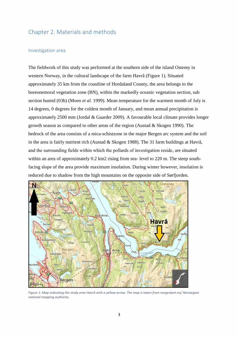
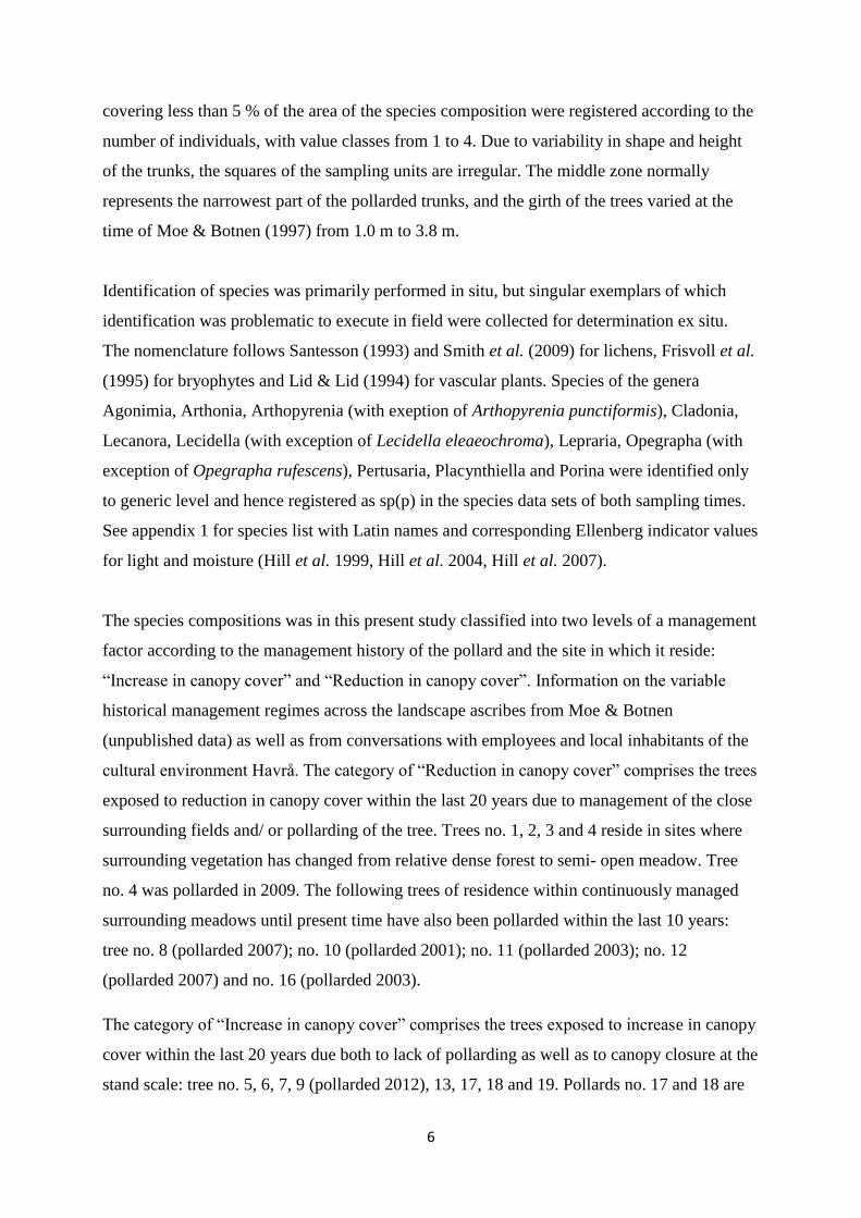
Figure 3: Pictures of pollards no. 13- west to the left and no. 10- south to the right.

Detrended Correspondence Analysis (DCA)

In order to reveal the structure of multivariate data sets, ordination methods seek to represent

the data along a reduced number of orthogonal axes. In decreasing order these axes represent

the main trends of the data. DCA ordination (Hill 1979, Hill & Gauch 1980) is a multivariate

indirect ordination technique based on a unimodal relation between species and environment,

i.e. based on the assumption of a unique set of optimal conditions for a species at which the

species has maximal abundance. A DCA ordination was performed on the two species

datasets from different sampling times employed in this study. Species situated close to each

other along the DCA ordination axis are similar in species abilities towards particular

8

environmental conditions. Environmental gradients in the species data are thereby revealed

from interpretation of the arrangement of species scores along each of the axes.

Strength of relation between variables

DCA axes, the moisture gradient and the light gradient were regressed on various predictor

variables (Table 2) and tested with Anova with F- test. The value of adjusted R- square from

the summary output signifies the strength of the relations. The moisture gradient is termed

“Moisture” and the light gradient is termed “Light”. “Height” and “Aspect” signifies

respectively gradients in height/ stem inclination and aspect. “Management” signifies

variation in historical management regime. “Sea” and “Moss Cover” means respectively

height above sea level/ distance from sea and total percentage of moss cover. The plots from

these regressions, indicating the correspondence between the environmental gradients in the

species data and predictor variables, were used as a support in the interpretation of the

quantified temporal trends in the species compositions as distributed along each axis and

gradients of light and moisture values.

Temporal turnover

DCA axes

The site scores of the sampling of Moe and Botnen (1997) were extracted from the site scores

of the sampling of this present study along each DCA axis. For each of the DCA axes, the

procedure for calculation of the mean temporal turnover can be illustrated through the

following expression: DCA change = Site ScoresT1 - SiteScoresT0

In order to evaluate whether the change is larger than what can be expected by random, the

significance of difference in time to the 4 different DCA change was tested through paired t-

tests.

Light and moisture gradients

The Null hypothesis of no difference in species optima values for light and moisture between

the sampling time of the original study and the sampling time of this study was tested through

applying a weighted average technique. Weighted averaging is a form of direct gradient

analysis. It shows only one axis and is useful for situations where only one primary

environmental gradient (at the time) is under consideration. The weighted average for light

was calculated for each species composition by multiplying the abundance of each species

9

times the Ellenberg light value for that species, whereby these values were summarized and

subsequently divided by the sum of species abundances. The resulting light ranking for the

species composition reflects its position along a light gradient. High light values correspond

to shade sensitive species, whereas low light values correspond to shade tolerant species.

Extracting the weighted light ranking of time 1 from that of time 2 for a species composition

provides a value for the temporal change in its weighted light ranking, corresponding to a

change in the position along the ordination gradient of light for that sample. The procedure

was repeated for Ellenberg moisture values. High moisture values correspond to draught

sensitive species, whereas low moisture values correspond to draught resistant species.

Measurements for obtaining the mean temporal change in the weighted light and moisture

ranking for all species compositions can be illustrated through the following expressions:

Lightchange = waEllenbergLightT1 - waEllenbergLightT0

Moisturechange = waEllenbergMoistureT1 - waEllenbergMoistureT0

Subsequently the significance of difference in time to the Lightchange and Moisturechange was

tested through paired t- tests.

Direction of temporal turnover

Positive Average Change value from the t- tests of DCA change (Table 3) indicates a

temporal compositional change towards increase in relative abundances of species with high

positive score along the DCA axis in question, in turn revealing temporal environmental

trends within the metacommunity at the scale of the landscape. Negative value signifies a

temporal trend in the epiphytic vegetation of increase in relative abundances of species

positioned at the negative end of the axis.

Positive Average Change value from the paired t- test of Lightchange indicates that the mean

temporal change in weighted light ranking along the gradient of light is positive. Such a

change would correspond to a temporal compositional change in direction of increase in

relative abundances of shade sensitive species and hence indicate an environmental trend of

increase in the availability of light. Negative value for Average Change corresponds to a

temporal change along the gradient towards an increase in relative abundances of shade

10

tolerant species and hence more shady conditions. Likewise, positive Average Change value

for Moisturechange indicates a temporal compositional change in direction of an increase in

relative abundances of draught sensitive species and more moist conditions, whereas negative

value implies a temporal increase in relative abundances of draught tolerant species and

reduced availability of moisture.

Rate of temporal turnover

Beta diversity can be conceived of as a measure of the degree of dissimilarity among sample

units as distributed along a gradient. Axes of DCA ordination are scaled in units of beta

diversity. The significance of a variable to variation in temporal turnover rate along a DCA

axis thus indicates the importance of that variable not only to the distribution of species

compositions along the axis, but also in structuring community response to temporal

environmental modification. The significance of the predictor variables of Aspect, Height and

Management to temporal turnover rates along DCA axes and to temporal change in weighted

light and moisture ranking was tested through mixed effect models with forward selection.

For all models fit to the data, AIC comparisons were performed in order to reveal whether or

not models including the tree factor as random factor in mixed effect models performed better

as compared to general linear models where the tree factor as random factor was omitted.

Based on these AIC comparisons, the tree factor was treated as random effect factor in the

linear mixed effect models employed, whereas Aspect, Height and Management were treated

as fixed effect factors. Below follows the model expression employed, with x representing the

predictor variables and “tree” representing the random factor:

Fit.x.lme <-lme (DCA change ~x, random=~1|tree)

Fit.x.lme <-lme (Light change ~x, random=~1|tree)

Fit.x.lme <-lme (Moisture change ~x, random=~1|tree)

Testing of the null hypotheses of no variation in temporal turnover rates along the different

variables was performed through Anova. I used forward selection to obtain the values for

each step of inclusion of variables in the model building. Graphical explorations were carried

out between response and predictor variables, and all predictors got into the selection

11

procedure of regression models. Full models included interaction terms. Akaike’s Information

Criterion (AIC; Burnham and Anderson 1998) was employed to obtain the most parsimonious

model (the minimal adequate linear mixed effect models; Zuur et al. 2009). Prior to

modelling, preliminary data exploration were performed. Editing and transforming of data

was performed in Microsoft Office Excel (Anonymous 2013). The data analyses were carried

out by R 2.15.3 (The R Development Core Team 2013) and by the R package “nlme”

(Pinheiro et al. 2011)

12

Chapter 3. Results

DCA

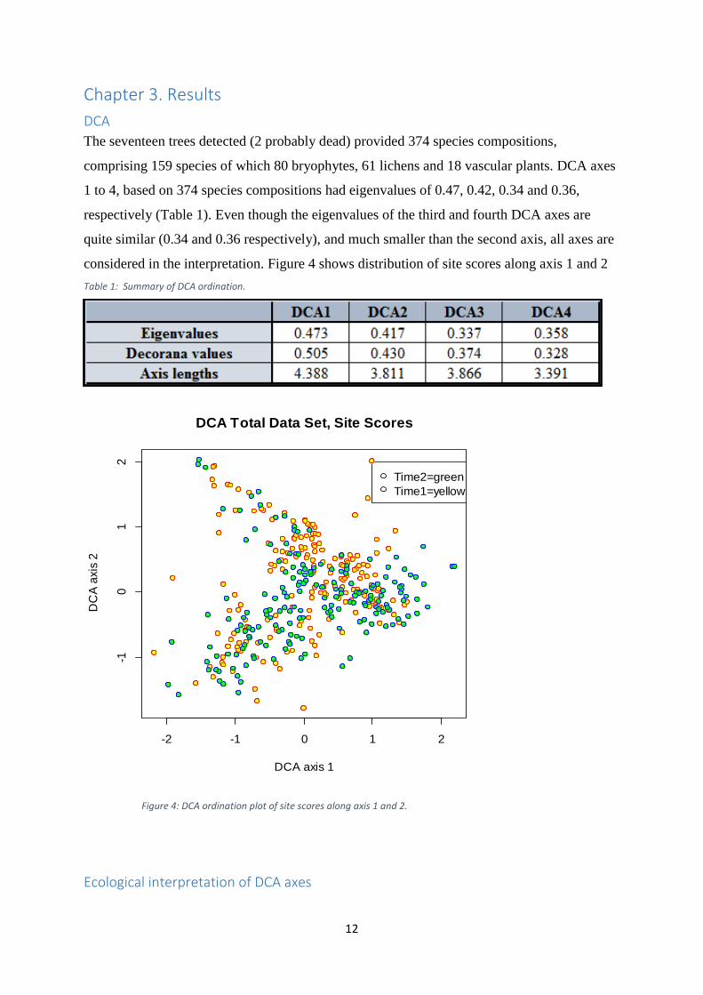
The seventeen trees detected (2 probably dead) provided 374 species compositions,

comprising 159 species of which 80 bryophytes, 61 lichens and 18 vascular plants. DCA axes

1 to 4, based on 374 species compositions had eigenvalues of 0.47, 0.42, 0.34 and 0.36,

respectively (Table 1). Even though the eigenvalues of the third and fourth DCA axes are

quite similar (0.34 and 0.36 respectively), and much smaller than the second axis, all axes are

considered in the interpretation. Figure 4 shows distribution of site scores along axis 1 and 2

Table 1: Summary of DCA ordination.

Figure 4: DCA ordination plot of site scores along axis 1 and 2.

Ecological interpretation of DCA axes

-2 -1 0 1 2

-10

12

DCA Total Data Set, Site Scores

DCA axis 1

DC

A a

xis

2

Time2=green

Time1=yellow

13

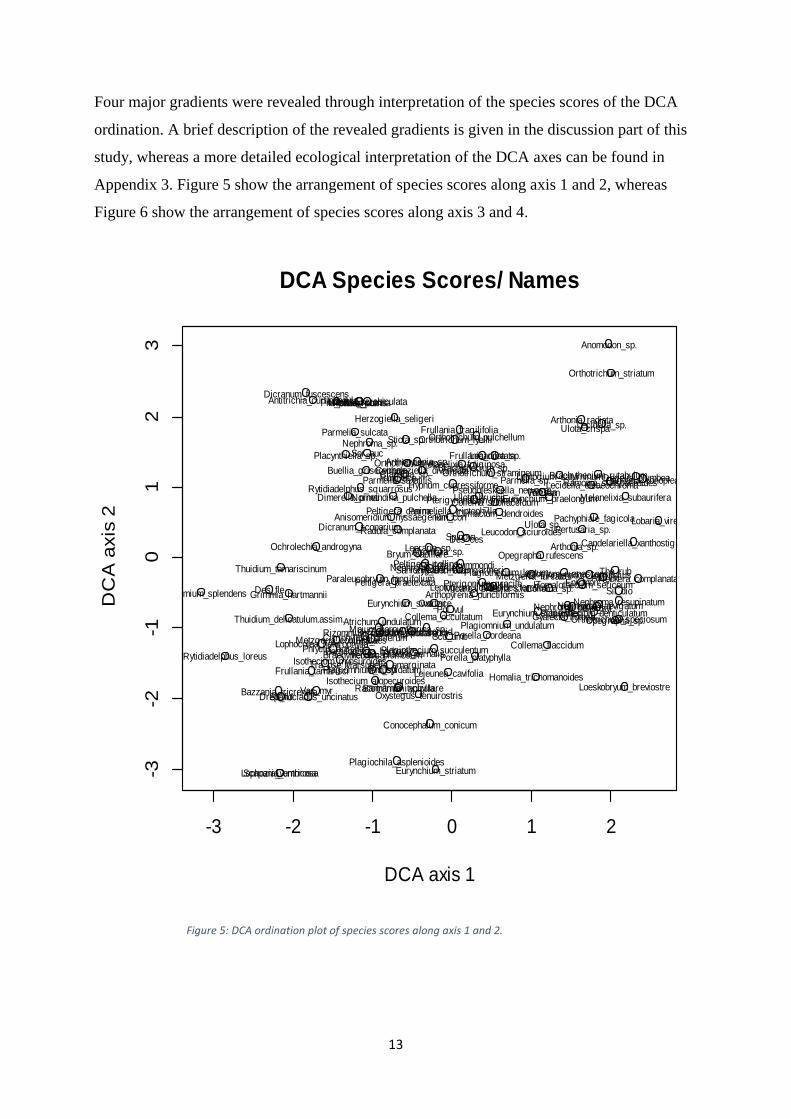
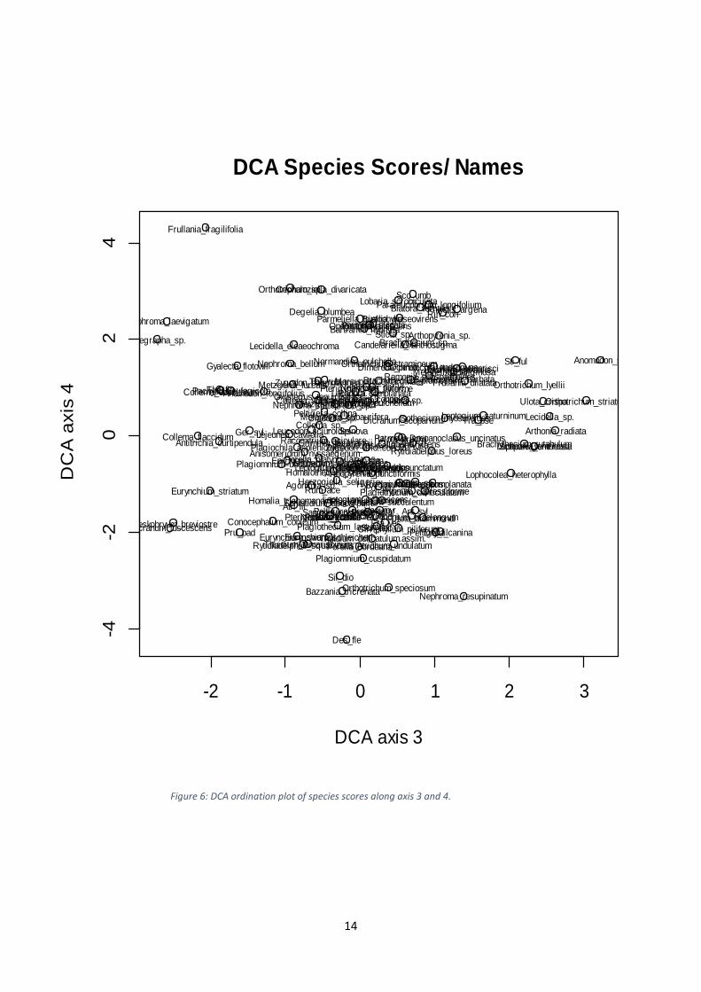
Four major gradients were revealed through interpretation of the species scores of the DCA

ordination. A brief description of the revealed gradients is given in the discussion part of this

study, whereas a more detailed ecological interpretation of the DCA axes can be found in

Appendix 3. Figure 5 show the arrangement of species scores along axis 1 and 2, whereas

Figure 6 show the arrangement of species scores along axis 3 and 4.

Figure 5: DCA ordination plot of species scores along axis 1 and 2.

-3 -2 -1 0 1 2

-3-2

-10

12

3

DCA Species Scores/ Names

DCA axis 1

DC

A a

xis

2

Anomodon_longifolius

Anomodon_sp.

Antitrichia_curtipendula

Atrichum_undulatum

Barbilophoza_barbata

Bartramia_ityphyllaBazzania_tricrenata

Brachythecium_plumosum

Brachythecium_rutabulumBrachythecium_sp.

Bryum_capillare

Cephaloziella_divaricata

Cirriphyllum_piliferum

Climacium_dendroides

Conocephalum_conicum

Dicranum_fuscescens

Dicranum_scoparium

Drepanocladus_uncinatus

Eurynchium_praelongum

Eurynchium_schleicheri

Eurynchium_striatum

Eurynchium_swartzii

Frullania_dilatata

Frullania_fragilifolia

Frullania_tamarisci

Grimmia_hartmannii

Herzogiella_seligeri

Homalia_trichomanoides

Homalothecium_sericeumHylocomium_splendens

Hypnum_cupressiforme

Isothecium_alopecuroides

Isothecium_myosuroides

Lejeunea_cavifolia

Leucodon_sciuroides

Loeskobryum_breviostre

Lophocolea_heterophylla

Lophozia_ventricosa

Marsupella_emarginata

Metzgeria_conjugata

Metzgeria_furcata

Mnium_hornum

Neckera_complanata

Neckera_pumila

Orthotrichum_sp.

Orthotrichum_lyelliiOrthotrichum_pulchellum

Orthotrichum_speciosum

Orthotrichum_stramineum

Orthotrichum_striatum

Oxystegus_tenuirostris

Paraleucobryum_longifolium

Plagiochila_asplenioides

Plagiomnium_cuspidatum

Plagiomnium_undulatum

Plagiothecium_denticulatum

Plagiothecium_laetum

Plagiothecium_succulentum

Pohlia_nutans

Porella_cordeana

Porella_platyphylla

Pseudoleskeella_nervosa

Pterigonium_gracile

Pterigynandrum_filiforme

Racomitrium_aciculare

Radula_complanata

Rizomnium_pseudopunctatum

Rytidiadelphus_loreus

Rytidiadelphus_squarrosus

Sanionia_uncinata

Scapania_umbrosa

Schistidium_apocarpum

Thuidium_delicatulum.assim.

Thuidium_tamariscinum

Ulota_bruchii

Ulota_crispa

Ulota_drummondi

Ulota_sp.

Zygodon_baumgartneri

Zygodon_virid..conoid.

Anisomeridium_nyssaegenum

Agonimia_sp.Arthonia_sp.

Arthonia_radiata

Arthopyrenia_punctiformis

Arthopyrenia_sp.

Biatora_vernalis

Buellia_griseovirens

Candelariella_xanthostigma

Cladonia_sp.

Collema_flaccidum

Collema_occultatum

Collema_subflaccidum

Collema_sp.

Degelia_plumbea

Dimerella_pineti

Gyalecta_flotowii

Lecanora_sp.

Lecidella_eleaeochroma

Lecidella_sp.

Lepraria_sp.

Leptogium_cyanescens

Leptogium_lichenoides.teretius.

Leptogium_saturninum

Lobaria_scrobiculata

Lobaria_virens

Melanelixia_fuliginosa

Melanelixia_subaurifera

Micarea_prasina_s.lat.

Nephroma_bellumNephroma_laevigatum

Nephroma_parile

Nephroma_resupinatum

Nephroma_sp.

Normandina_pulchella

Ochrolechia_androgyna

Opegrapha_sp.

Opegrapha_rufescens

Pachyphiale_fagicola

Pannaria_conopleaParmelia_saxatilis

Parmelia_sulcata

Parmelia_sp.

Parmeliella_triptophylla

Peltigera_collina

Peltigera_canina

Peltigera_praetextata

Pertusaria_sp.

Phlyctis_argena

Placynthiella_sp.

Porina_sp.

Ramonia_subspaeroides

Rin_con

Rin_fla

Sco_umb

Sti_ful

Sticta_sp.

The_fla

The_rub

Tra_pseAnt_syl

Ath_fil

Cam_rot

Des_ces

Des_fle Dry_fil Epi_mon

Fra_ves

Ger_sylOxa_ace

Pol_vul

Pru_pad

Rum_ace

Sil_dio

Sor_auc

Vac_myr

Val_sam

Veronica

Sp.nova

14

-2 -1 0 1 2 3

-4-2

02

4

DCA Species Scores/ Names

DCA axis 3

DC

A a

xis

4 Anomodon_longifolius

Anomodon_sp.

Antitrichia_curtipendula

Atrichum_undulatum

Barbilophoza_barbata

Bartramia_ityphylla

Bazzania_tricrenata

Brachythecium_plumosum

Brachythecium_rutabulum

Brachythecium_sp.

Bryum_capillare

Cephaloziella_divaricata

Cirriphyllum_piliferum

Climacium_dendroides

Conocephalum_conicumDicranum_fuscescens

Dicranum_scoparium

Drepanocladus_uncinatus

Eurynchium_praelongum

Eurynchium_schleicheri

Eurynchium_striatum

Eurynchium_swartzii

Frullania_dilatata

Frullania_fragilifolia

Frullania_tamarisci

Grimmia_hartmannii

Herzogiella_seligeri

Homalia_trichomanoides

Homalothecium_sericeum

Hylocomium_splendensHypnum_cupressiforme

Isothecium_alopecuroides

Isothecium_myosuroides

Lejeunea_cavifoliaLeucodon_sciuroides

Loeskobryum_breviostre

Lophocolea_heterophylla

Lophozia_ventricosa

Marsupella_emarginata

Metzgeria_conjugata

Metzgeria_furcata

Mnium_hornum

Neckera_complanata

Neckera_pumila

Orthotrichum_sp.

Orthotrichum_lyellii

Orthotrichum_pulchellum

Orthotrichum_speciosum

Orthotrichum_stramineum

Orthotrichum_striatumOxystegus_tenuirostris

Paraleucobryum_longifolium

Plagiochila_asplenioides

Plagiomnium_cuspidatum

Plagiomnium_undulatum

Plagiothecium_denticulatum

Plagiothecium_laetum

Plagiothecium_succulentum

Pohlia_nutans

Porella_cordeana

Porella_platyphylla

Pseudoleskeella_nervosa

Pterigonium_gracile

Pterigynandrum_filiforme

Racomitrium_aciculare

Radula_complanata

Rizomnium_pseudopunctatum

Rytidiadelphus_loreus

Rytidiadelphus_squarrosus

Sanionia_uncinata

Scapania_umbrosa

Schistidium_apocarpum

Thuidium_delicatulum.assim.Thuidium_tamariscinum

Ulota_bruchii

Ulota_crispa

Ulota_drummondi

Ulota_sp.

Zygodon_baumgartneri

Zygodon_virid..conoid.Anisomeridium_nyssaegenum

Agonimia_sp.

Arthonia_sp.

Arthonia_radiata

Arthopyrenia_punctiformis

Arthopyrenia_sp.

Biatora_vernalisBuellia_griseovirens

Candelariella_xanthostigma

Cladonia_sp.

Collema_flaccidum

Collema_occultatumCollema_subflaccidum

Collema_sp.

Degelia_plumbea

Dimerella_pinetiGyalecta_flotowii

Lecanora_sp.

Lecidella_eleaeochroma

Lecidella_sp.

Lepraria_sp.

Leptogium_cyanescens

Leptogium_lichenoides.teretius.

Leptogium_saturninum

Lobaria_scrobiculata

Lobaria_virens

Melanelixia_fuliginosa

Melanelixia_subaurifera

Micarea_prasina_s.lat.

Nephroma_bellum

Nephroma_laevigatum

Nephroma_parile

Nephroma_resupinatum

Nephroma_sp.

Normandina_pulchellaOchrolechia_androgyna

Opegrapha_sp.

Opegrapha_rufescens

Pachyphiale_fagicolaPannaria_conoplea

Parmelia_saxatilis

Parmelia_sulcata

Parmelia_sp.

Parmeliella_triptophylla

Peltigera_collina

Peltigera_canina

Peltigera_praetextata

Pertusaria_sp.

Phlyctis_argena

Placynthiella_sp.Porina_sp.

Ramonia_subspaeroides

Rin_con

Rin_fla

Sco_umb

Sti_ful

Sticta_sp.

The_flaThe_rub

Tra_pse

Ant_sylAth_fil

Cam_rotDes_ces

Des_fle

Dry_fil

Epi_mon

Fra_ves

Ger_syl

Oxa_ace

Pol_vul

Pru_pad

Rum_ace

Sil_dio

Sor_auc

Vac_myr

Val_sam

Veronica

Sp.nova

Figure 6: DCA ordination plot of species scores along axis 3 and 4.

15

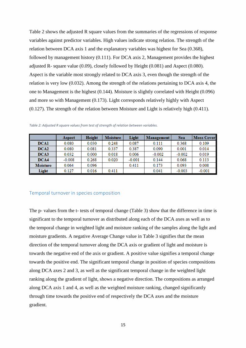
Table 2 shows the adjusted R square values from the summaries of the regressions of response

variables against predictor variables. High values indicate strong relation. The strength of the

relation between DCA axis 1 and the explanatory variables was highest for Sea (0.368),

followed by management history (0.111). For DCA axis 2, Management provides the highest

adjusted R- square value (0.09), closely followed by Height (0.081) and Aspect (0.080).

Aspect is the variable most strongly related to DCA axis 3, even though the strength of the

relation is very low (0.032). Among the strength of the relations pertaining to DCA axis 4, the

one to Management is the highest (0.144). Moisture is slightly correlated with Height (0.096)

and more so with Management (0.173). Light corresponds relatively highly with Aspect

(0.127). The strength of the relation between Moisture and Light is relatively high (0.411).

Table 2: Adjusted R square values from test of strength of relation between variables.

Temporal turnover in species composition

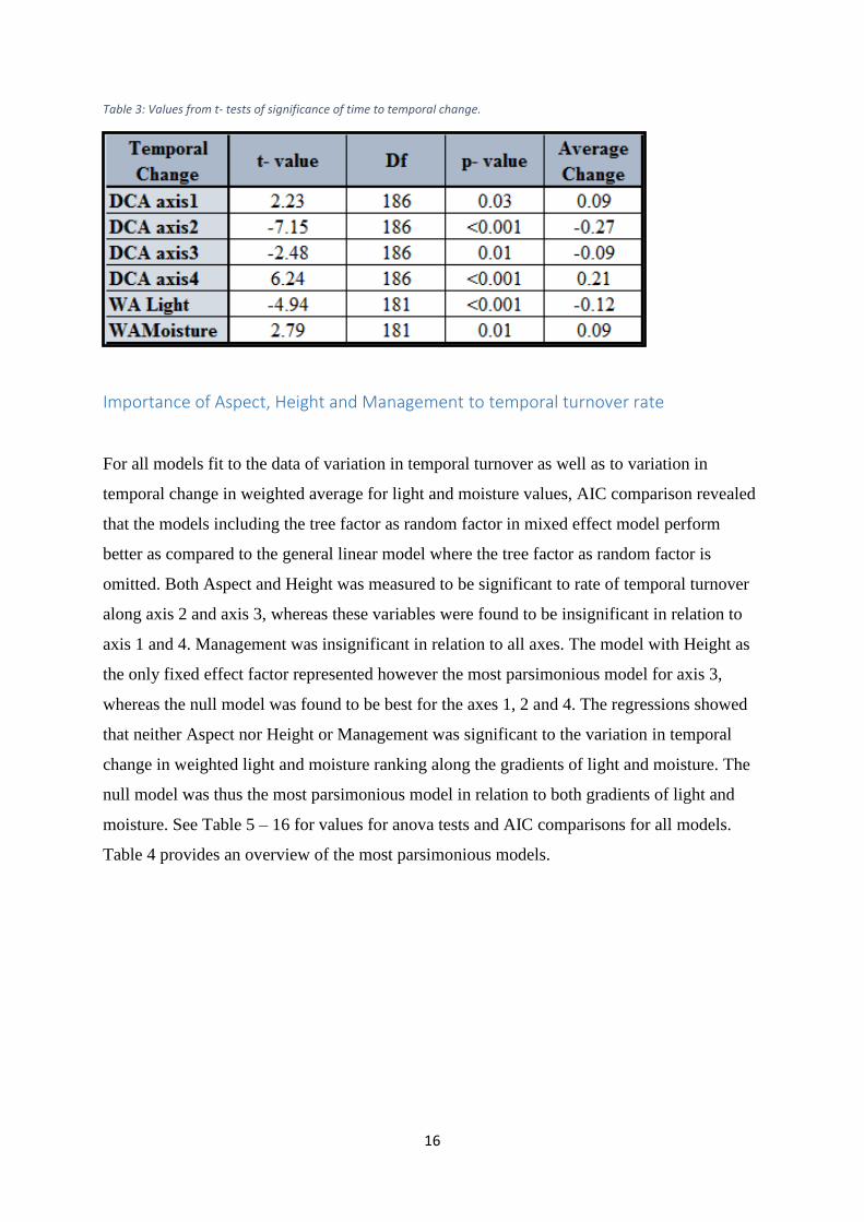
The p- values from the t- tests of temporal change (Table 3) show that the difference in time is

significant to the temporal turnover as distributed along each of the DCA axes as well as to

the temporal change in weighted light and moisture ranking of the samples along the light and

moisture gradients. A negative Average Change value in Table 3 signifies that the mean

direction of the temporal turnover along the DCA axis or gradient of light and moisture is

towards the negative end of the axis or gradient. A positive value signifies a temporal change

towards the positive end. The significant temporal change in position of species compositions

along DCA axes 2 and 3, as well as the significant temporal change in the weighted light

ranking along the gradient of light, shows a negative direction. The compositions as arranged

along DCA axis 1 and 4, as well as the weighted moisture ranking, changed significantly

through time towards the positive end of respectively the DCA axes and the moisture

gradient.

16

Table 3: Values from t- tests of significance of time to temporal change.

Importance of Aspect, Height and Management to temporal turnover rate

For all models fit to the data of variation in temporal turnover as well as to variation in

temporal change in weighted average for light and moisture values, AIC comparison revealed

that the models including the tree factor as random factor in mixed effect model perform

better as compared to the general linear model where the tree factor as random factor is

omitted. Both Aspect and Height was measured to be significant to rate of temporal turnover

along axis 2 and axis 3, whereas these variables were found to be insignificant in relation to

axis 1 and 4. Management was insignificant in relation to all axes. The model with Height as

the only fixed effect factor represented however the most parsimonious model for axis 3,

whereas the null model was found to be best for the axes 1, 2 and 4. The regressions showed

that neither Aspect nor Height or Management was significant to the variation in temporal

change in weighted light and moisture ranking along the gradients of light and moisture. The

null model was thus the most parsimonious model in relation to both gradients of light and

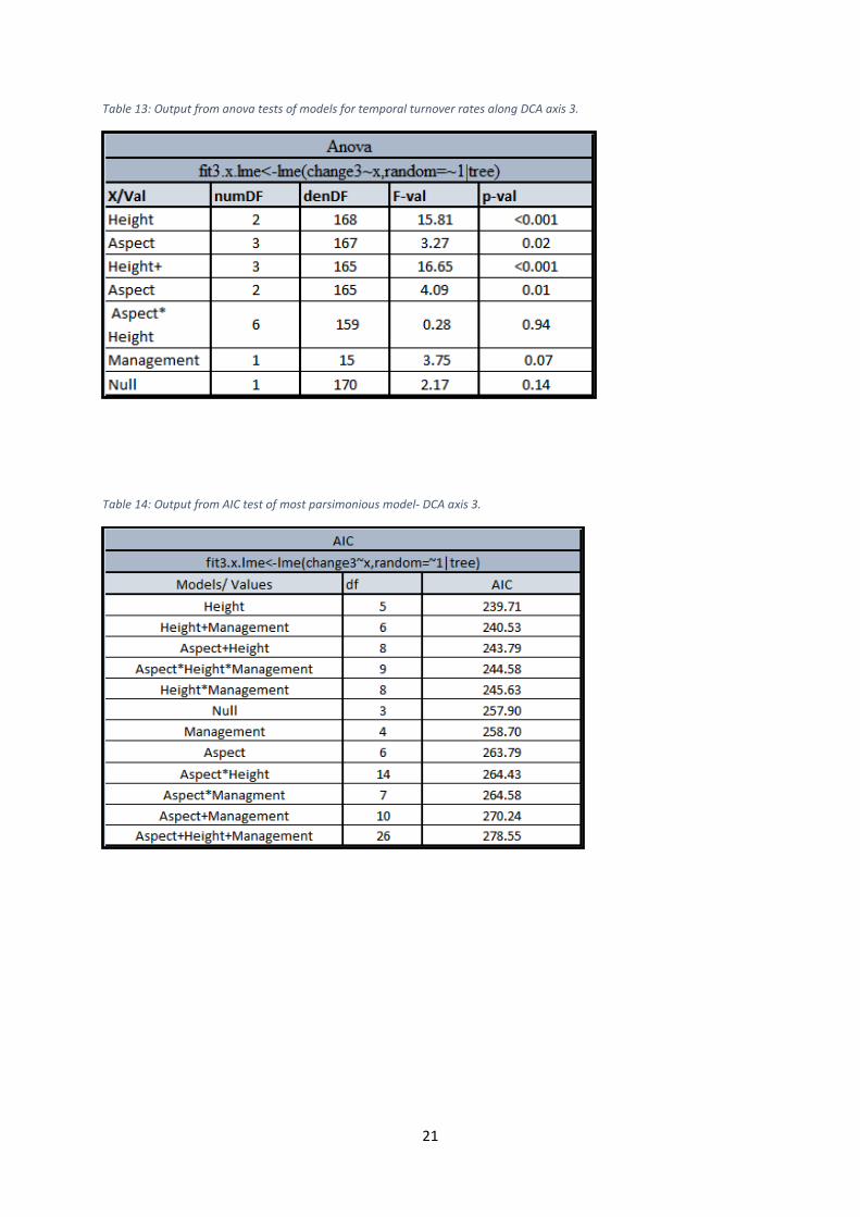
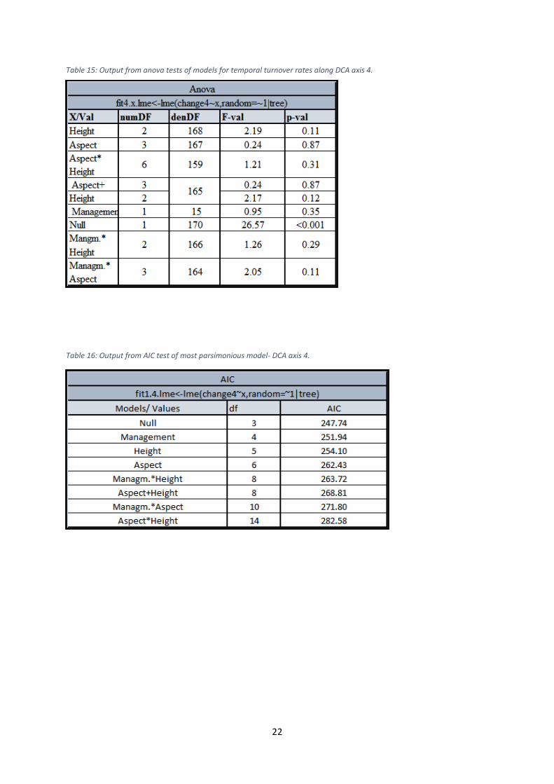
moisture. See Table 5 – 16 for values for anova tests and AIC comparisons for all models.

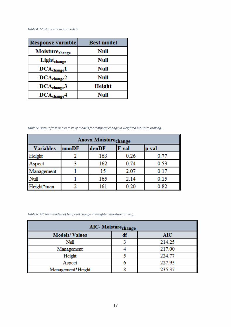
Table 4 provides an overview of the most parsimonious models.

17

Table 4: Most parsimonious models.

Table 5: Output from anova tests of models for temporal change in weighted moisture ranking.

Table 6: AIC test- models of temporal change in weighted moisture ranking.

18

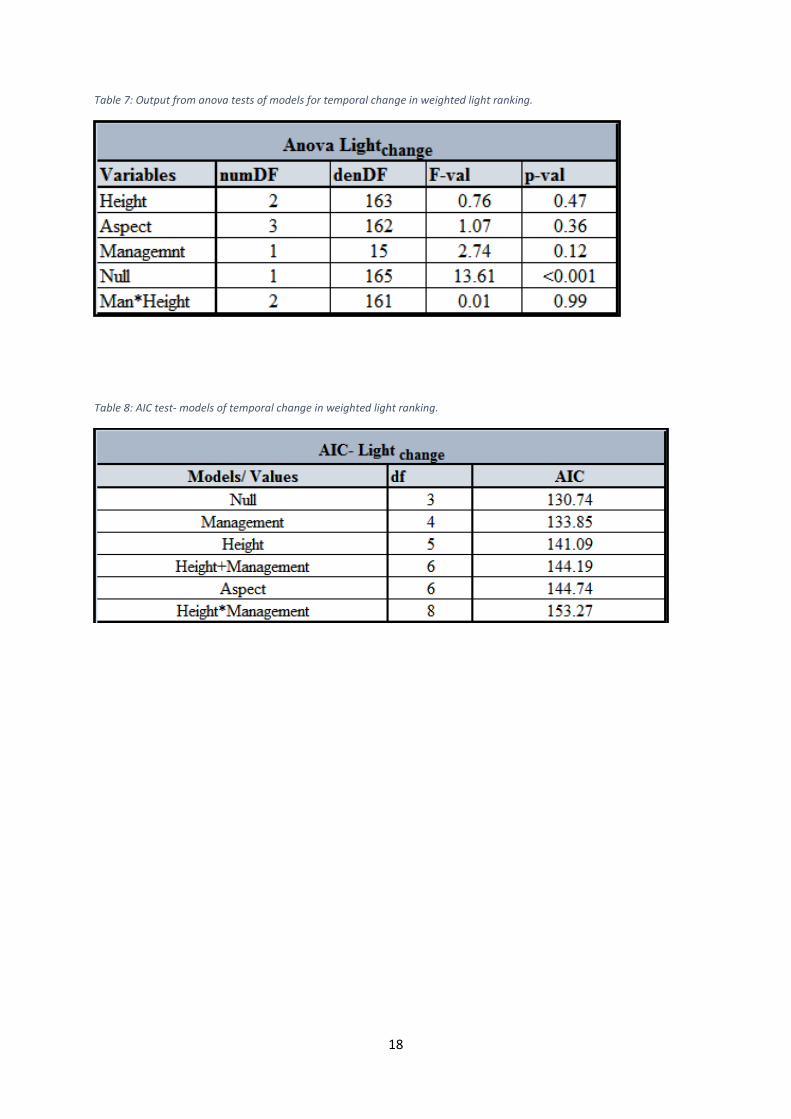
Table 7: Output from anova tests of models for temporal change in weighted light ranking.

Table 8: AIC test- models of temporal change in weighted light ranking.

19

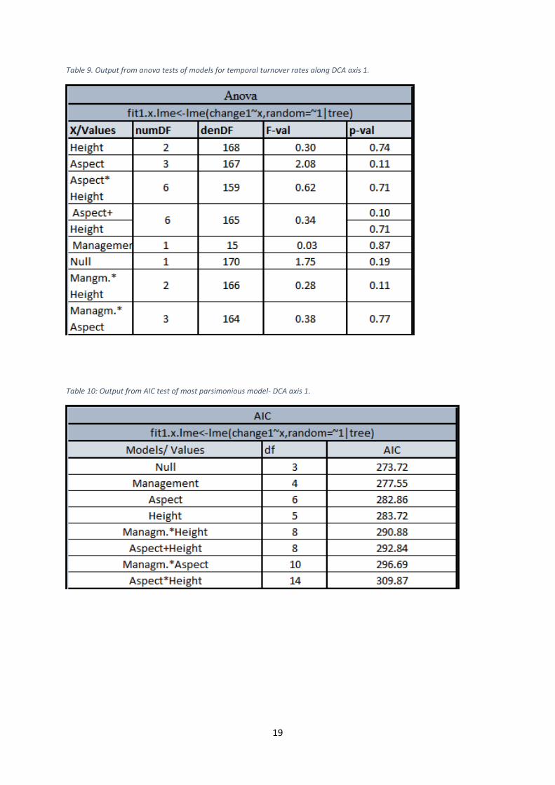
Table 9. Output from anova tests of models for temporal turnover rates along DCA axis 1.

Table 10: Output from AIC test of most parsimonious model- DCA axis 1.

20

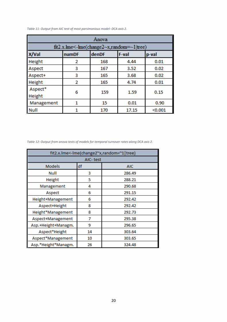
Table 11: Output from AIC test of most parsimonious model- DCA axis 2.

Table 12: Output from anova tests of models for temporal turnover rates along DCA axis 2.

21

Table 13: Output from anova tests of models for temporal turnover rates along DCA axis 3.

Table 14: Output from AIC test of most parsimonious model- DCA axis 3.

22

Table 15: Output from anova tests of models for temporal turnover rates along DCA axis 4.

Table 16: Output from AIC test of most parsimonious model- DCA axis 4.

23

Chapter 4. Discussion

Main results

The results from the paired t- tests (Table 3) demonstrate the significance of time to change in

species composition from the sampling time of the original study to the sampling time of this

present study along all DCA axes, as well as to change in the weighted light and moisture

ranking. Consequently, during the last 20 years, the composition of the epiphytic communities

on pollarded trunks of Fraxinus excelsior at Havrå has changed significantly in relation to

availability of light and moisture.

Interpretation of species scores along DCA axis 2 and DCA axis 4 indicates that these axes

explain much of the directional spatial change in community structure in the species data of

this study. The direction of the temporal turnover as interpreted along these axes are therefore

likely to indicate the overall direction of the change in composition of the epiphytic

metacommunity of this study through time. Both DCA axis 2 and DCA axis 4 seems to

represent a distribution trend along the stem. Species similar in abilities towards moisture as

well as light correspond to a particular height and aspect along DCA axis 2, whereas DCA

axis 4 separates species differing in their morphological adaptations towards retention of

water. The direction of temporal turnover as distributed along DCA axis 2 and 4, as well as

along the gradients in light and moisture, indicates a trend in the epiphytic vegetation towards

homogenization of the within- tree variation in species composition at the expense of shade

sensitive species. This trend in the epiphytic metacommunity corresponds to an environmental

trend towards more shady and humid conditions at the scale of the landscape.

Historical management regime of the pollards and surrounding meadows has no significant

effect on the rate of the compositional change through time, whereas temporal turnover rates

along axis 2 vary significantly with Height and Aspect. The corresponding regression plots

indicate a relatively higher rate of temporal turnover in the top zone and to the aspect of south

where assemblages of shade sensitive species reside, as compared to the basal zone and the

aspect of north. This result indicates that the temporal turnover in large is driven by a higher

species response to change in availability of light and moisture within assemblages of shade

sensitive species tolerant or sensitive to draught, as compared to assemblages of shade

tolerant species more or less sensitive to draught.

24

The results from the testing of the effect of Aspect, Height and Management on the rates of

temporal turnover thus support the indication from the measured direction of temporal

turnover that abandoned management is a driver of compositional change through time in the

epiphytic communities of this study, at the expense of shade sensitive species.

Before discussing the direction and nature of temporal turnover as distributed along DCA

axes and gradients in light and moisture, in the following I describe the different DCA axes

briefly (see Appendix 3 for a complete interpretation of species scores along each DCA axis).

Interpretation of DCA axes

DCA axis 1

At the positive end of axis 1 reside species found within the lowermost sites of the study area,

e.g. Gyalecta flotowii, Thelopsis rubella, Leucodon sciuroides, Homalothecium sericeum,

Degelia plumbea and Lobaria virens. Ochrolechia androgyna, Scapania umbrosa and

Lophozia ventricosa have high negative score on axis 1 and are restricted to one or two trunks

at 185 m altitude (Moe & Botnen 1997). The arrangement of species along axis 1 (Appendix

3) thus suggests a (non- directional) variance in community structure between sites within the

lowermost situated areas of high site quality and short distance to the sea/ farm buildings, and

sites within the uppermost areas of poorer site quality with longer distance to the sea. The

kind of beta diversity along DCA axis 1 seems thus to reflect variation in the identities of

species among species compositions within the study area, and not beta diversity as turnover

in species composition (cf. Legendre et al. 2005; Anderson et al. 2011). The plots from the

regression of DCA axis 1 on Sea and Management (highest R2, see table 2) show that the

negative end of the axis corresponds to the uppermost level of the study area and sites of

increase in canopy cover. These results from the test of strength of relation between variables

thus support the ecological interpretation of the species scores along axis 1.

DCA axis 2

At the positive end of DCA axis 2 reside shade sensitive and draught tolerant species like

Antitrichia curtipendula, Orthotrichum pulchellum, Orthotrichum lyelli, Orthotrichum

striatum, Parmelia sulcata, Lobaria scrobiculata, and Pseudoleeskella nervosa (Figure 5).

Species typical of the lower, negative end of the axis are shade resistant/ draught sensitive

species like Loeskobryum breviostre, Plagiochila asplenioides, Plagiothecium denticulatum,

25

Collema flaccidum and Eurynchium striatum. DCA axis 2 seems thus to represent a

distribution trend along the stem, with species similar in abilities towards moisture as well as

light corresponding to a particular Height (Appendix 3). This arrangement of species might as

well represent a gradient of aspect, with the positive end corresponding to the aspects of south

and west were irradiation and evaporation is likely to be higher than to the north and east.

Plots of the regressions of DCA axis 2 on explanatory variables and gradients of light and

moisture show that the basal part, the aspect of north, low light values (shade tolerant species)

and high moisture values (draught sensitive species) correspond to the negative end of DCA

axis 2. These plots also show that the top zone, south, high light values (shade sensitive

species) and low moisture values (draught tolerant species) correspond to the positive end of

axis 2. Results from tests of strength of relation between variables (Table 2) thus support the

ecological interpretation of the arrangement of species scores along axis 2.

DCA axis 3

The arrangement of species along DCA axis 3 (Appendix 3) seems to reflect a non-

directional gradient that may be explained by different substrate conditions on the trunk, what

suggests that DCA axis 3 represent conditions related to the cyclical successive stages of the

epiphytic vegetation. The difference in substrate conditions seem however to correspond to

different heights along the trunk, what suggests differences in peeling- off rates along the

gradient of height (Appendix 4). The strengths of all the relation between DCA axis 3 and

predictor variables are low, and no clear trend of moisture or light availability was revealed

along DCA axis 3.

Due to more windy environments in the upper parts of the trunk and to the aspect of south in

open meadows (Appendix 3), re- colonization of the trunk after each peeling-off by the

cryptogamic epiphytes at Havrå is likely to happen at a higher rate within the top zone and to

the aspect of south (Appendix 4). Variation in cyclical successive stages may thus underlie the

measured significance of Aspect and Height to temporal turnover rates along axis 3, as well as

the result of the model with Height as predictor as the most parsimonious model related to

axis 3. Differences in exposure may explain the higher turnover rates in the top zone and to

the south relative to the other levels of height and aspect, as shown from regression plots. The

results related to axis 3 illustrate the way structural properties of the habitat interacts with

environment in producing spatial variation in stages in the cyclical succession in communities

26

of sessile organisms residing in dynamic habitats, like epiphytes residing on old trunks in

open environments.

DCA axis 4

Axis 4 seems to represent a gradient of height/ stem inclination followed by variation in the

degree to which species adhere to their substrate, i.e. a gradient of morphological adaptations

towards retention of water along the trunk (Appendix 3). The plot from the regression of DCA

axis 4 on Height shows a correspondence between the top and middle zone and the positive

end of axis 4 where species of the genera Orthotrichum, Leidella elaeochroma, Parmelia

sulcata, Opegrapha rufescens and Phlyctis argena reside. These species adhere more or less

strongly to their substrate as opposed to species positioned at the negative end of axis 4,

which press loosely against their substrate, like Nephroma resupinatum, Peltigera

resupinatum, Bazzania tricrenata, Loeskobryum breviostre and Thuidium tamariscinum. The

negative end corresponds to the basal zone, and the results from the regression thus support

the ecological interpretation of the arrangement of species along axis 4. The regression plot

also indicates high similarity among top and middle zone with respect to environmental

factors and floristic composition in relation to the basal zone (cf. Moe & Botnen 1997).

In the following interpretations of the direction and rate of the temporal turnover, focus is on

the directional gradients identified along DCA axis 2 and DCA axis 4, as well as on the

gradients of light and moisture.

Direction of temporal turnover.

Temporal trends revealed along gradients in light and moisture

The negative direction of the significant temporal change along the light gradient (Table 3)

implies that the temporal change in composition of the epiphytic communities consist in an

increase in relative abundances of shade tolerant species, corresponding to an increase in

resemblance to the composition at the north side (highest R2 with Aspect, Table 2). A positive

direction of the significant temporal change along the moisture gradient implies that the

temporal change in composition of the epiphytic communities consist in an increase in

relative abundances of draught sensitive species. This temporal trend in the epiphytic

vegetation correspond to an increase in resemblance to the composition of sites of increase in

27

canopy cover as well as to the basal part of the trunk (highest R2 with Management and

Height, Table 2). A relatively strong relation (R2 = 0.411) between Light and Moisture

suggests that the gradients of light and moisture explain much of the same variation in the

species compositions of this study, and the direction of temporal turnover as distributed along

these gradients suggests a temporal environmental trend of more shady and moist conditions.

Temporal trends revealed along DCA axis 2

The direction of the significant temporal turnover as distributed along axis 2 towards the

negative end of the axis (Table 3) indicates a change towards species compositions of the

lower parts of the trunk and at the north side. This direction of the compositional change

corresponds to an increase in relative abundances of draught sensitive and shade tolerant

species, like Plagiochila asplenioides, Eurynchium striatum and Conocephalum conicum, as

well as to a decrease in shade sensitive species like cyanolichens and old- growth indicators

like Antitrichia curtipendula. This structural change in the metacommunity indicates a trend

in the local environment of higher availability of moisture (from atmospheric humidity and/ or

precipitation) and lower availability of light, and speak as such in favour of abandoned

management as a driver of change in the epiphytic community.

Temporal trends revealed along DCA axis 4

The direction of the significant temporal change in community structure along DCA axis 4

towards the positive end (Table 3) indicates a trend in the species data towards resemblance to

species compositions of the mid/ upper parts, towards sites of increase in canopy cover and

finally towards decrease in moss cover. These trends may indicate an increase in species

moderately pressed towards their substrate and which reside throughout the entire trunk and/

or thrive within environmental conditions provided by the middle zone/ overhanging upper

zone of the trunk characterized by a low percentage of moss cover, like species of the genera

Agonimia; Arthonia and Lepraria, Radula complanata, Plagiomnium undulatum,

Plagiothecium denticulatum, Metzgeria furcata, M. conjugata, Neckera complanata, Hypnum

cupressiforme, Micarea prasina.s.lat., and Nephroma parile.

The trend revealed along axis 4 indicate more shady local environments with reduced

moisture from precipitation, corresponding to the overhanging top zones and the middle part

of the trunk. These results in turn suggest that the trend of increase in moist conditions found

28

along DCA axis 2 and the gradient of moisture is likely to in large derive from increase in

atmospheric humidity following canopy closure rather than increase in moisture from

precipitation.

Variation in temporal turnover rates

DCA axis 4

The indication of the direction of temporal turnover as distributed along DCA axis 4 towards

homogenization of species compositions along the gradient of stem inclination seems to be

supported through the testing of Height on temporal turnover rates along the axis. Even

though Height was not significant to temporal turnover rates along DCA axis 4, the plot from

this regression shows that the highest response is found in the basal and top zones, where

species respectively loosely and strongly pressed to their substrate reside. This pattern thus

corresponds to a decrease both in large, draught sensitive pleurocarps residing in the basal

part as well as in shade sensitive and draught sensitive species residing in the upper zones of

90 degrees (like cyanolichens, cf. DCA axis 2 in Appendix 3).

The process of homogenization in species compositions and environments of light and

moisture at the fine scale along the stem illustrates the way the gradients of aspect and height

becomes less important to the vertical distribution of epiphytes as canopy grow denser,

corresponding to a lower variation in community responses to environments of light and

moisture. Such a decrease in beta diversity throughout the stem following an extended period

of dense canopy cover was indicated through regression plots showing a lower variation

within unmanaged sites among rates of temporal turnover along axis 2 as function of Aspect

and Height, as compared to a high variation within managed sites.

DCA axis 2

The overall significance of Aspect and Height, and insignificance of Management, to turnover

rates along axis 2 indicates however that differences in access to light and moisture

throughout the trunk are important to the vertical distribution of epiphytes despite increase in

canopy cover. Limitation of light in this study seems therefore not to be sufficient to mask the

effect of neither height nor aspect (cf. Barkman 1958; Kenkel & Bradfield 1981; Pirintsos et

al. 1993; Moe & Botnen 1997, 2000; Marmor et al. 2012). The null model represented

however the most parsimonious model for axis 2, implying that Height and Aspect does not

29

have predictive power in relation to rates of temporal turnover in the epiphytic communities

of this study (cf. Appendix 4).

Assemblages of shade sensitive species were interpreted through their arrangement along

DCA axis 2 (Appendix 3) to reside within the upper parts of the trunk and to the aspect of

south. Consequently, a larger effect of reduced availability of light and moisture is expected

within these zones as compared to the north side and the basal zone. The plots from the

regressions of temporal turnover rates along axis 2 on Aspect and Height, showing that the

rate of compositional turnover is highest in the top zone and to the aspect of south, thus

confirms this expectation.

In combination with the measured direction of temporal turnover along DCA axis 2, DCA

axis 4 and the gradients in light and moisture, the results from the model testing thus supports

the interpretation of an increase in canopy cover following abandoned management as driver

of compositional change through time in the epiphytic communities of this study. This study

thus demonstrate a decline in relative abundances of assemblages consisting of shade and

draught sensitive cyanolichens, old- growth indicators like Antitrichia curtipendula, as well as

other shade sensitive epiphytes like Melanelixia fuliginosa, Orthotrichum striatum, O. lyelli,

O. pulchellum, Pseudoleeskella nervosa, Pteridynandrum filiforme and Ulota crispa. The

results indicate that this temporal trend in shade sensitive species reflects a negative response

to abandoned management during the last 20 years.

Uncertainties

Due to its use in this study for comparison among assemblages within the same vegetation

type (cryptogam epiphytes), the employment of Ellenberg indicator values for assessment of

temporal trends in the vegetation in relation to environment can be considered as reliable (cf.

Wamelink et al. 2002). The reliability of the weighted average technique employed in this

study is in addition supported through the equivalence of its results to the trends revealed

along DCA axes 2 and 4 discussed in the following.

Relationships between current epiphyte occurrence patterns and the historical landscape

structure have suggested more than century long time- lags (Ellis & Coppins 2007; Johansson

et al. 2012). Ranius et al. (2008) claims that as old trees represent a long- lasting habitat, it

might be likely that current epiphytic species distribution patterns may reflect the historical

30

habitat quality. Johansson et al. (2013) demonstrated a great time lag in the response of shade

sensitive species to environmental changes. A great time lag in the response of the epiphytic

vegetation in this study to management would potentially overestimate the effect of

abandoned management, with the consequence that the documented decline in shade sensitive

species in this study would be exaggerated.

Management implications

In many European woodlands, negative impacts from cessation of pollarding on epiphytic and

saproxylic biodiversity have recently been documented (Leppik et al. 2011; Jönsson et al.

2011; Marmor et al. 2012; Johanson et al. 2013; Sebek et al. 2013). There is as such

mounting evidence for the need to mitigate the negative impact of overgrowth on the future

viability of epiphytic cryptogams as well as micro- organisms residing on old trees and

adapted to light open environments within the cultural landscape through pollarding and

management of surrounding meadows. Jönsson & Thor (2012) showed that traditionally

managed open wooded meadows had the highest incidence of ash dieback disease, followed

by significantly higher risk of species extinction, compared with unmanaged closed forests

and semi-open grazed sites. Ash dieback disease as such impose yet another factor to the

assumed additive effects of agricultural change and silvicultural practices to the future

viability of the shade sensitive old- forest epiphytes throughout Europe in general, and to the

shade sensitive epiphytic vegetation of this study in particular.

Several of the pollards at Havrå are currently dying due to high age and/ or lack of pollarding.

Increasing the viability of the host trees through pollarding, as well as recruitment of new

trees, is thus in addition to management of surrounding vegetation a prerequisite to mitigate

the temporal trend in relative abundances of shade sensitive epiphytes residing on the pollards

at Havrå measured in this study to be negative.

31

Chapter 5. Concluding remarks

A negative impact of abandoned management on the temporal trend in an assemblage of

shade sensitive cryptogam epiphytes residing on old trees in a traditionally light- open

landscape was indicated through the results in this study. These results thus add to an

amounting body of evidence for an ongoing and future decline within the cultural landscape

in shade sensitive epiphytic bryophytes and lichens dependent on long continuity. In order to

understand to what degree this trend represents an actual threat to the future viability of rare,

obligate epiphytes within this group, further research is needed for assessing the way forestry

and ash dieback disease add to the declining course of the successional trajectories of such

species within the traditionally light- open cultural landscape.

Quantifying temporal turnover in species compositions along environmental gradients and

measuring temporal change in species optimum values for light and moisture gradients at the

fine scale revealed processes that is likely to be less detectable through addressing uniquely

the spatial component of turnover and/ or courser spatial scales. The results of this study

demonstrate that the combination of approaches employed is operational and conceptually

relevant for detecting trends in old- growth epiphytic bryophytes and lichens dependent on

light- open forested landscapes, in relation to environmental modifications at the scale of the

landscape. The results also speak in favour of using communities of epiphytic bryophytes and

lichens in detection of temporal environmental trends at the scale of the landscape.

32

33

References

Anderson, M. J., Crist, T. O., Chase, J. M., Vellend, M., Inouye, B. D., Freestone, A. L.,

Sanders, N. J., Cornell, H. V., Comita, L. S., Davies, K. F., Harrison, S. P., Kraft, N. J. B.,

Stegen, J. C., Swenson, N. G. 2011. Navigating the multiple meanings of beta diversity: a

roadmap for the practicing ecologist. Ecology Letters 14: 19–2.

Austad, I. & Skogen, A., 1988. Havråtunet i Osterøy kommune. En botanisk-økologisk

analyse og en plan for istandsetting og skjøtsel av kulturlandskapet. Økoforsk rapp. 13, 119

(in Norwegian).

Austad, I. & Skogen, A. 1990. Restoration of a deciduous woodland in W Norway formerly

used for fodder production: effects on tree canopy and floristic composition. Vegetatio 88 p.1-

20.

Barkman, J. J. 1958. Phytosociology and Ecology of Cryptogamic Epiphytes. Van Gorkum &

Company. Assen, Netherlands.

Bates, J. W. 1992. Influence of chemical and physical factors on Quercus and Fraxinus

epiphytes at Loch Sunart, western Scotland: a multivariate analysis. Journal of Ecology

80:163–179.

Bendiksen, E., Brandrud. T.E. & Røsok, Ø. (Ed.), Framstad, E., Gaarder, G., Hofton, T.H.,

Jordal, J.B., Klepsland, J.T. & Reiso, S. 2008. Boreale lauvskoger i Norge. Naturverdier og

udekket vernebehov. – NINA Rapport 367. In Norwegian

Büdel, B., Vivas, M., Lange, O. L. 2013. Lichen species dominance and the resulting

photosynthetic behaviour of Sonoran Desert soil crust types (Baja California, Mexico).

Ecological processes 2:6. doi: 10.1186/2192-1709-2-6

Burnham, K.P., Anderson, D.R. 1998. Model selection and Inference: A practical

Information- Theoretic Approach. (Springer- Verlag. New York).

Chase, J., Myers, J. A. 2011. Disentangling the importance of ecological niches from

stochastic processes across scales. Phil. Trans. Soc. B. 366. doi: 10.1098/rstb.2011.0063

Ecological Society of America. 2000. Dispersal limitations of epiphytic lichens result in

species. Ecological Applications 10 (3): 789–799.

Ellenberg, H., Weber, H.E., Duell, R., Wirth, V., Werner, W. & Pauliszen, D. 1992.

Zeigerwerte von Pflanzen in Mitteleuropa. Scripta Geobot. Göttingen 18: 1-258.

Ellis, C.J., Coppins, B.J., Hollingsworth, P.M. 2012. Tree fungus: Lichens under threat from

ash dieback. Nature 491 (672). doi: 10.1038/491672a

Ellis, J. Christopher. 2012. Lichen epiphyte diversity: A species, community and trait- based

review. Perspectives in Plant Ecology, Evolution and Systematics 14: 131-152.

34

Frisvoll, A., Elvebakk, A., Flatberg, K.I. & Økland, R.H. 1995. Sjekkliste over norske mosar.

NINA. Temahefte 4: 1–101.

Gauslaa, Y. & Ohlson, M. 1997. Et historisk perspektiv på kontinuitet og forekomst av

epifyttiske laver i norske skoger. – Blyttia 55: 15-27. (In Norwegian)

Green, T. G. A., Nash, T. H. III & Lange, O. L. 2008. Physiological ecology of carbon

dioxide exchange. In: Nash, T. H. III (ed.), Lichen biology: 152–181. Cambridge University

Press, Cambridge

Hill, M.O. & Gauch, H.G. Jr. 1980. Detrended correspondence analysis: an improved

ordination technique. Vegetation 42: 47-58

Hill, M.O. 1979. DECORANA – A fortran program for detrended correspondence analysis

and reciprocal averaging. Cornell University, Ithaca, New York, USA

Hill, M.O., Mountford, J.O., Roy, D.B. & Bunce, R.G.H. 1999. Ellenberg's indicator values

for British plants. ECOFACT 2, Technical annex. Institute of Terrestrial Ecology,

Huntingdon, UK.

Hill, M. O., Preston, C. D. & Roy, D.B. 2004. Attributes of British and Irish Plants: Status,

Size, Life History, Geography and Habitats. PLANTATT.

Hill, M.O., Preston, C. D., Bosanquet, S.D.S., Roy, D.B. 2007. BRYOATT Attributes of

British and Irish Mosses, Liverworts and Hornworts With Information on Native Status, Size,

Life Form, Life History, Geography and Habitat.

Johanson P. 2006. Lichen diversity and its conservation in deciduous forests and wooded

meadows on Gotland, Sweden. In: Nordic Council of ministers. Nordplus neighbor project.

“Monitoring lichens – monitoring with lichens” Workshop in Lithuania, May 11-16, 2006

“Conservation of lichen rich biotopes and endangered species.

Johansson, V. 2012. Distribution and Persistence of Epiphyte Metapopulations in Dynamic

Landscapes. Doctoral Thesis. Acta Universitatis agriculturae Sueciae 17.

Johansson, V., Ranius, T., Snäll, T. 2013. Epiphyte metapopulation persistence after drastic

habitat decline and low tree regeneration: time-lags and effects of conservation actions.

Journal of Applied Ecology 50 (2): 414–422.

Jordal, J. B. og Gaarder, G. 2009. Supplerande kartlegging av biologisk mangfald i jordbruket

sitt kulturland- skap, inn- og utmark i Hordaland, med ei vurdering av kunnskapsstatus.

Direktoratet for naturforvaltning, Utgreiing 2009-1.

Jönsson, M. T., Thor, G. & Johansson, P. 2011. Environmental and historical effects on lichen

diversity in managed and unmanaged wooded meadows. Applied Vegetation Science 14(1):

120–131.

35

Jönsson, M.T., Thor, G. 2012. Estimating Coextinction Risks from Epidemic Tree Death:

Affiliate Lichen Communities among Diseased Host Tree Populations of Fraxinus excelsior.

PLoS ONE 7(9): e45701. doi:10.1371/journal.pone.0045701

Jüriado, I., Liira, J. & Paal, J. 2009. Diversity of epiphytic lichens in boreo-nemoral forests on

the North-Estonian limestone encarpment: the effects of tree level factors and local

environmental conditions. Lichenologist 41:81–94.

Jüriado, I., Karu, L., Lira, J. 2012. Habitat conditions and host tree properties affect the

occurrence, abundance and fertility of the endangered lichen Lobaria pulmonaria in wooded

meadows of Estonia. The Lichenologist 44(2): 263–276. doi:10.1017/S0024282911000727

Kenkel, N. C. & Bradfield, G. E. 1981. Ordination of epiphytic bryophyte communities in a

wet- temperate coniferous forest, South-Coastal British Columbia. Vegetation 45: 147–154.

Kenkel, N. C. & Bradfield, G. E. 1986. Epiphytic vegetation on Acer macrophyllum: a

multivariate study of species-habitat relation- ships. Vegetatio 68: 43–53.

Király, I., Nascimbene, J., Tinya, F., Ódor, P. 2013. Factors influencing epiphytic bryophyte

and lichen species richness at different spatial scales in managed temperate forests.

Biodiversity and Conservation 22(1): 209-223, DOI: 10.1007/s10531-012-0415-y.

Kopecky, M., Hedl, R., Szab, P. 2013. Non-random extinctions dominate plant community

changes in abandoned coppices. Journal of Applied Ecology. doi: 10.1111/1365-2664.12010.

Lange, O. L., Kilian, E., Ziegler, H. 1986. Water vapor uptake and photosynthesis of lichens:

performance differences in species with green and blue-green algae as phycobionts.

Oecologia 71:104-110.

Legendre, P., Borcard, D., Peres-Neto, P.R. 2005. Analyzing beta diversity: partitioning the

spatial variation of community composition data. Ecol. Monogr. 75: 435–450.

Leppik, E. & Jüriado, I. 2008. Factors important for epiphytic lichen communities in wooded

meadows of Estonia. Folia Cryptog Estonica 44:75–87.

Leppik, E., Jüriado, I & Liira, J. 2011. Changes in stand structure due to cessation of

traditional land use in wooded meadows impoverish epiphytic lichen communities. The

Lichenologist 43(3): 257-274.

Marmor, L., Tõrra, T. & Randlane, T. 2010: The vertical gradient of bark pH and epiphytic

macrolichen biota in relation to alkaline air pollution. Ecological Indica- tors 10: 1137–1143.

Marmor, L., Tõrra, T., Saag, L., Randlan, T. 2012. Species Richness of Epiphytic Lichens in

Coniferous Forests: the Effect of Canopy Openness. Annales Botanici Fennici, 49(5): 352-

358, DOI: http://dx.doi.org/10.5735/085.049.0606

Lid, J. & Lid, D. T. 1994. Norsk flora. Det Norske Samlaget. Oslo.

36

Moen, A., Elven, R. & Odland, A. 1999. Vegetation section map of Norway. National Atlas

of Norway. Norwegian Mapping Authority.

Moe, B. & Botnen, A. 1997. A quantitative study of the epiphytic vegetation on pollarded

trunks of Fraxinus excelsior at Havrå, Osterøy, W Norway. - Pl. Ecol. 129: 157-177.

Moe, B. & Botnen, A. 2000. Epiphytic vegetation on pollarded trunks of Fraxinus excelsior in

four different habitats at Grinde, Leikanger, W Norway. - Pl. Ecol. 151: 143-159.

Nedkvitne, K., Gjerdåker, J. 1993. Ask i norsk natur og tradisjon. Norsk Skogbruksmuseum.

Elverum.

Nilsson, S.G. Arup, U., Baranowski, R. & Ekman, S. 1994. Trädbundna lavar och skalbaggar

i ålderdomliga kulturlanskap. – Svensk bot. Tidskr. 88: 1-12.

Nordbakken, J.-F. & Austad, I. 2010. Styvingstrær, nøkkelbiotoper i norsk natur - en

undersøkelse av moser på almestuver Ulmus glabra i Sogn og Fjordane. Blyttia 68: 245-255.

Ódor, P., Király, I., Tinya, F., Bortignon, F., Nascimbene, J. 2013. Patterns and drivers of

species composition of epiphytic bryophytes and lichens in managed temperate forests. Forest

Ecology and Management 306: 256-265. DOI: 10.1016/j.foreco.2013.07.001

Oksanen, J., Kindt, R., Legendre, P. & O'Hara, B. 2007. Package 'vegan' Version 1.9-13.

Univ. of Oulu, Oulu.

Palmqvist, K., Dahlman, L., Jonsson, A., Nash, T. H. 2008: The carbon economy of lichens.

In: Nash, T. H. (ed.), Lichen biology: 182–215. Cambridge University Press, Cambridge

Phillips 1959

Piippo, S. 1982. Epiphytic bryophytes as climatic indicators in Eastern Fennoscandia. Acta

Botanica Fennica 119: 1–39.

Pinheiro, J., Bates, D., DebRoy, S., Sarkar, D., R Development Core Team. 2011. nlme:

Linear and Nonlinear Mixed Effects Models. R package version 3.1-98, URL,

http://CRAN.R-project.org/package=nlme

Pirintsos, S. A., Diamantopoulos, J. & Stamou, G. P. 1993. Analysis of the vertical

distribution of epiphytic lichens on Pinus nigra (Mount Olympos, Greece) along an altitudinal

gradient. Vegetatio 109: 63–70.

Ranius, T., Eliasson, P., Johansson, P. 2008. Large-scale occurrence patterns of red-listed

lichens and fungi on old oaks are influenced both by current and historical habitat density.

Biodivers Conserv 17:2371–2381. DOI 10.1007/s10531-008-9387-3

R Development Core Team. 2013. R: A Language and Environment for Statistical

Computing. R Foundation for Statistical Computing, Vienna, Austria. ISBN 3-900051-07-0,

URL, http://www.R-project.org/.

37

Rose, F. 1992. Temperate forest management: its effect on bryophyte and lichen floras and

habitats, pp 211-233. In Bates, J. W & Farmer, A.M. (Ed.) 1992. Bryophytes and lichens in a

changing environment. Claredon Press, London.

Rose, F. 1993. Ancient British woodlands and their epiphytes. British Wildlife 5: 83–93.

Santesson, R. 1993. The lichens and lichenicolous fungi of Sweden and Norway. SBT-

forlaget, Lund.

Sebek, P., Altman, J., Platek, M., Cizek, L. 2013. Is Active Management the Key to the

Conservation of Saproxylic Biodiversity? Pollarding Promotes the Formation of Tree

Hollows. PLoS ONE 8(3): e60456. doi:10.1371/journal.pone.0060456

Sillett, S.C., Antoine, M.E. 2004. Lichens and Bryophytes in Forest Canopies. In

Lowman, M.D., Rinker, H.B. 2004. Forest Canopies. Second Edition. Elsevier Academic

Press, London.

Sjøgren, E. 1995. Changes in the epilithic and epiphytic moss cover in two deciduous forest

areas on the island of Öland (Sweden) – a comparison between 1958–1962 and 1988–1990.

Studies in Plant Ecology 19: 1–106.

Smith, C.W., Aptroot, A., Coppins, B.J., Fletcher, A., Gilbert, O.L., James, P.W.,Wolseley,

P.A. (eds.). 2009. The lichens of Great Britain and Ireland, British Lichen Society, London.

Stegen, J. C., Freestone, A. L., Crist, T. O., Anderson, M. J., Chase, J. M., et al. 2012.

Stochastic and deterministic drivers of spatial and temporal turnover in breeding bird

communities. Global Ecol Biogeogr. 22: 202–212

Timdal E., Bratli, H.,Holien, H. & Tønsberg, T. 2010. Lav (Lichenes) in Kålås, J.A., Viken,

Å., Henriksen, S. and Skjelseth, S. (Ed.) 2010. The 2010 Norwegian Red List for Species.

Norwegian Biodiversity Information Centre, Norway. Available at:

http://www.artsdatabanken.no/Article.aspx?m=268&amid=8237

Tønsberg, T., Gauslaa, Y., Haugan, R., Holien, H. & Timdal, E. 1996. The threatened

macrolichens of Norway – 1995.- Sommerfeltia 23: 1-258. ISBN 82-7420-029-2. ISSN 0800-

6865

Wamelink, G. W. W., Joosten, V., van Dobben, H. F., Berendse, F. 2002. Validity of

Ellenberg indicator values judged from physico-chemical field measurements. Journal of

Vegetation Science 13: 269-278.

Zuur, A., Ieno, E.N., Walker, N., Saveliev, A.A., Smith, G.M. 2009. Mixed Effects Models

and Extensions in Ecology with R. Springer, New York (574 pp).

38

39

Figures Figure 1: Map showing the study area. Havrå is indicated with a yellow arrow. The map is taken from

norgeskart.no/ Norwegian national mapping authority. ........................................................................ 3

Figure 2: Stem inclination interacts with height on the trunk. The drawing is taken from Moe &

Botnen (1997). ......................................................................................................................................... 5

Figure 3: Pictures of pollards no. 13- west to the left and no. 10- south to the right. ........................... 7

Figure 4: DCA ordination plot of site scores along axis 1 and 2. ........................................................... 12

Figure 5: DCA ordination plot of species scores along axis 1 and 2. ..................................................... 13

Figure 6: DCA ordination plot of species scores along axis 3 and 4. ..................................................... 14

Tables Table 1: Summary of DCA ordination. .................................................................................................. 12

Table 2: Adjusted R square values from test of strength of relation between variables. ..................... 15

Table 3: Values from t- tests of significance of time to temporal change. ........................................... 16

Table 4: Most parsimonious models. ..................................................................................................... 17

Table 5: Output from anova tests of models for temporal change in weighted moisture ranking. ..... 17

Table 6: AIC test- models of temporal change in weighted moisture ranking. ..................................... 17

Table 7: Output from anova tests of models for temporal change in weighted light ranking. ............ 18

Table 8: AIC test- models of temporal change in weighted light ranking. ............................................ 18

Table 9. Output from anova tests of models for temporal turnover rates along DCA axis 1. .............. 19

Table 10: Output from AIC test of most parsimonious model- DCA axis 1. .......................................... 19

Table 11: Output from AIC test of most parsimonious model- DCA axis 2. .......................................... 20

Table 12: Output from anova tests of models for temporal turnover rates along DCA axis 2. ............ 20

Table 13: Output from anova tests of models for temporal turnover rates along DCA axis 3. ............ 21

Table 14: Output from AIC test of most parsimonious model- DCA axis 3. .......................................... 21

Table 15: Output from anova tests of models for temporal turnover rates along DCA axis 4. ............. 22

Table 16: Output from AIC test of most parsimonious model- DCA axis 4. .......................................... 22

Table 17: Species list with Ellenberg indicator values. .......................................................................... 40

Table 18: UTM positions, height above sea level and diameter at breast height.. ............................... 44

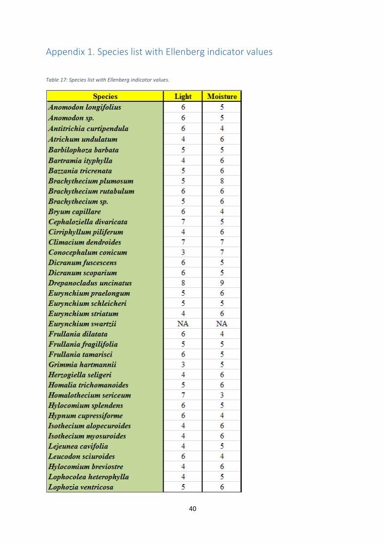
40

Appendix 1. Species list with Ellenberg indicator values

Table 17: Species list with Ellenberg indicator values.

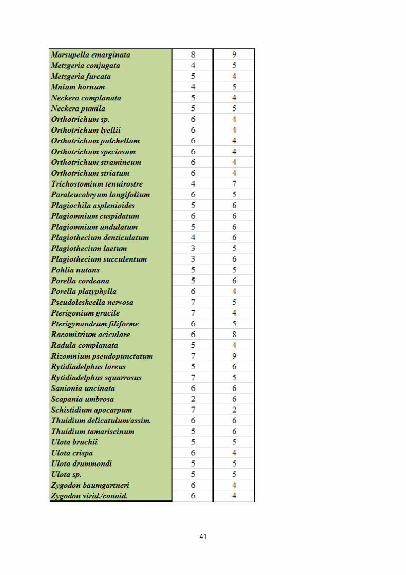
41

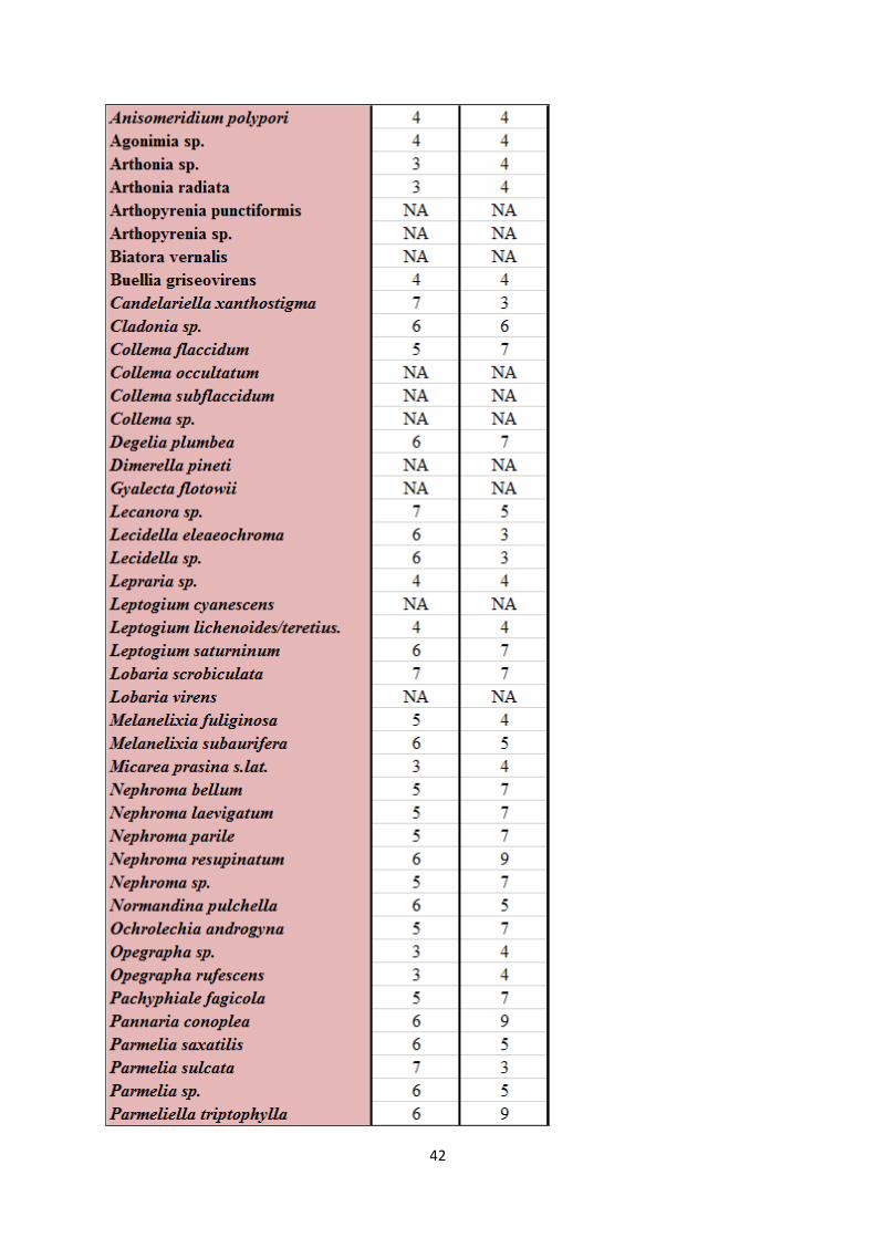
42

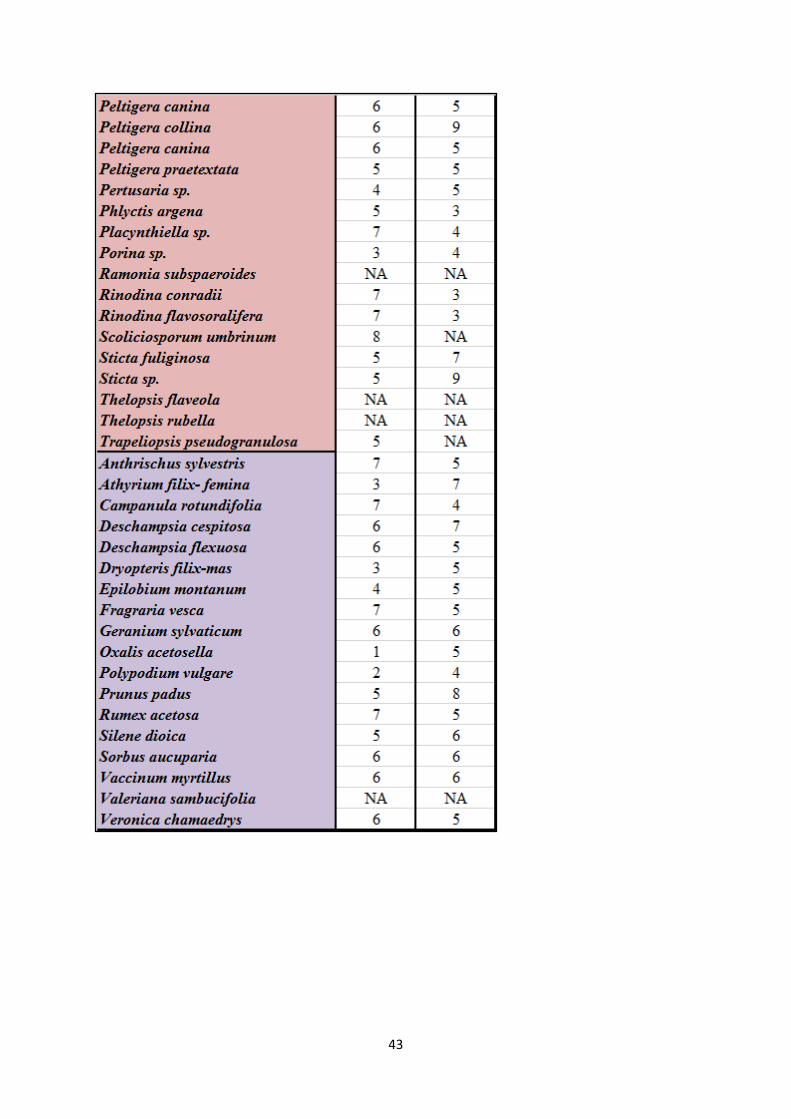
43

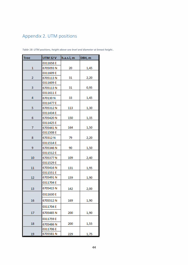
44

Appendix 2. UTM positions

Table 18: UTM positions, height above sea level and diameter at breast height..

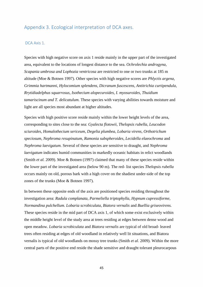
45

Appendix 3. Ecological interpretation of DCA axes.

DCA Axis 1.

Species with high negative score on axis 1 reside mainly in the upper part of the investigated

area, equivalent to the locations of longest distance to the sea. Ochrolechia androgyna,

Scapania umbrosa and Lophozia ventricosa are restricted to one or two trunks at 185 m

altitude (Moe & Botnen 1997). Other species with high negative scores are Phlyctis argena,

Grimmia hartmanni, Hylocomium splendens, Dicranum fuscescens, Antitrichia curtipendula,

Rrytidiadelphus squarrosus, Isothecium alopecuroides, I. myosuroides, Thuidium

tamariscinum and T. delicatulum. These species with varying abilities towards moisture and

light are all species most abundant at higher altitudes.

Species with high positive score reside mainly within the lower height levels of the area,

corresponding to sites close to the sea: Gyalecta flotowii, Thelopsis rubella, Leucodon

sciuroides, Homalothecium sericeum, Degelia plumbea, Lobaria virens, Orthotrichum

speciosum, Nephroma resupinatum, Ramonia subspheroides, Lecidella elaeochroma and

Nephroma laevigatum. Several of these species are sensitive to draught, and Nephroma

laevigatum indicates humid communities in markedly oceanic habitats in relict woodlands

(Smith et al. 2009). Moe & Botnen (1997) claimed that many of these species reside within

the lower part of the investigated area (below 90 m). The red- list species Thelopsis rubella

occurs mainly on old, porous bark with a high cover on the shadiest under-side of the top

zones of the trunks (Moe & Botnen 1997).

In between these opposite ends of the axis are positioned species residing throughout the

investigation area: Radula complanata, Parmeliella triptophylla, Hypnum cupressiforme,

Normandina pulchellum. Lobaria scrobiculata, Biatora vernalis and Buellia griseovirens.

These species reside in the mid part of DCA axis 1, of which some exist exclusively within

the middle height level of the study area at trees residing at edges between dense wood and

open meadow. Lobaria scrobiculata and Biatora vernalis are typical of old broad- leaved

trees often residing at edges of old woodland in relatively well lit situations, and Biatora

vernalis is typical of old woodlands on mossy tree trunks (Smith et al. 2009). Within the more

central parts of the positive end reside the shade sensitive and draught tolerant pleurocarpous

46

mosses Homalothecium sericeum, Pterigonium gracile, Pterigynandrum filiforme,

Pseudoleeskella nervosa and Leucodon sciuroides.

Moe & Botnen (1997) found the age of pollarded branches to be lowest near the farm

buildings (15 years for the youngest at that time), and the branches further away from the

farm centre to be the oldest (60 years at the most). During the time between the sampling of

Moe & Botnen (1997) and the sampling of this study, this pattern of level of pollarding was

reinforced. The trees most close to the farm have been pollarded within the last 10 years (with

exception of the pollarded tree nr. 16 situated at high altitude), whereas the trees situated in

areas more distant from the farm have been left unpollarded. Even though there is higher site

quality (the capacity of the field to produce wood) in the lower sites close to the sea (Kjetil

Monstad, personal communication 05.05.2013), there is no clear trend of tree girth within the

area. The higher site quality in the lowermost area may however interfere with the gradient

revealed along axis 1 as effect of that bark pH/ nutrient status may be modified by an

interaction with the soil environment.

DCA Axis 2

Examples of species which reside in the upper, positive part of axis 2 are Antitrichia

curtipendula, Orthotrichum pulchellum, Orthotrichum lyelli, Orthotrichum striatum, Ulota

crispa, Parmelia sulcata, Lecidella eleaeochroma, Lobaria scrobiculata, Pseudoleeskella

nervosa, Frullania fragilifolia, Orthotrichum stramineum, Dicranum fuscesence and

Cephaloziella divaricata. Within the upper mid part of the axis, among others, species

sensitive to both shade and draught are found: Nephroma resupinatum, Parmeliella

triptophylla, Lobaria scrobiculata, Leptogium saturninum, Pannaria conoplea, Sanionia

uncinata, Peltigera collina, Brachythecium rutabulum, Climacium dendroides and Degelia

plumbea. Example of species from the middle part of the axis with tolerance towards shade

and draught are: Metzgeria furcata, Radula complanata, Leptogium lichenoides/ terretius,

Neckera complanata, Opegrapha rufescence. Species typical of the lower, negative part of the

axis are shade resistant/ draught sensitive species like Loeskobryum breviostre, Oxystegus

tenuirostris, Plagiochila asplenioides, Plagiothecium denticulatum, Plagiothecium

succulentum, Rytidiadelphus loreus, Collema flaccidum, Eurynchium striatum and

Conocephalum conicum.

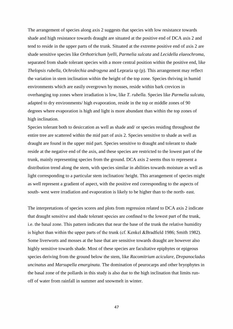
47

The arrangement of species along axis 2 suggests that species with low resistance towards

shade and high resistance towards draught are situated at the positive end of DCA axis 2 and

tend to reside in the upper parts of the trunk. Situated at the extreme positive end of axis 2 are

shade sensitive species like Orthotrichum lyelli, Parmelia sulcata and Lecidella elaeochroma,

separated from shade tolerant species with a more central position within the positive end, like

Thelopsis rubella, Ochrolechia androgyna and Lepraria sp (p). This arrangement may reflect

the variation in stem inclination within the height of the top zone. Species thriving in humid

environments which are easily overgrown by mosses, reside within bark crevices in

overhanging top zones where irradiation is low, like T. rubella. Species like Parmelia sulcata,

adapted to dry environments/ high evaporation, reside in the top or middle zones of 90

degrees where evaporation is high and light is more abundant than within the top zones of

high inclination.

Species tolerant both to desiccation as well as shade and/ or species residing throughout the

entire tree are scattered within the mid part of axis 2. Species sensitive to shade as well as

draught are found in the upper mid part. Species sensitive to draught and tolerant to shade

reside at the negative end of the axis, and these species are restricted to the lowest part of the

trunk, mainly representing species from the ground. DCA axis 2 seems thus to represent a

distribution trend along the stem, with species similar in abilities towards moisture as well as

light corresponding to a particular stem inclination/ height. This arrangement of species might

as well represent a gradient of aspect, with the positive end corresponding to the aspects of

south- west were irradiation and evaporation is likely to be higher than to the north- east.

The interpretations of species scores and plots from regression related to DCA axis 2 indicate

that draught sensitive and shade tolerant species are confined to the lowest part of the trunk,

i.e. the basal zone. This pattern indicates that near the base of the trunk the relative humidity

is higher than within the upper parts of the trunk (cf. Kenkel &Bradfield 1986; Smith 1982).

Some liverworts and mosses at the base that are sensitive towards draught are however also

highly sensitive towards shade. Most of these species are facultative epiphytes or epigeous

species deriving from the ground below the stem, like Racomitrium aciculare, Drepanocladus

uncinatus and Marsupella emarginata. The domination of peurocarps and other bryophytes in

the basal zone of the pollards in this study is also due to the high inclination that limits run-

off of water from rainfall in summer and snowmelt in winter.

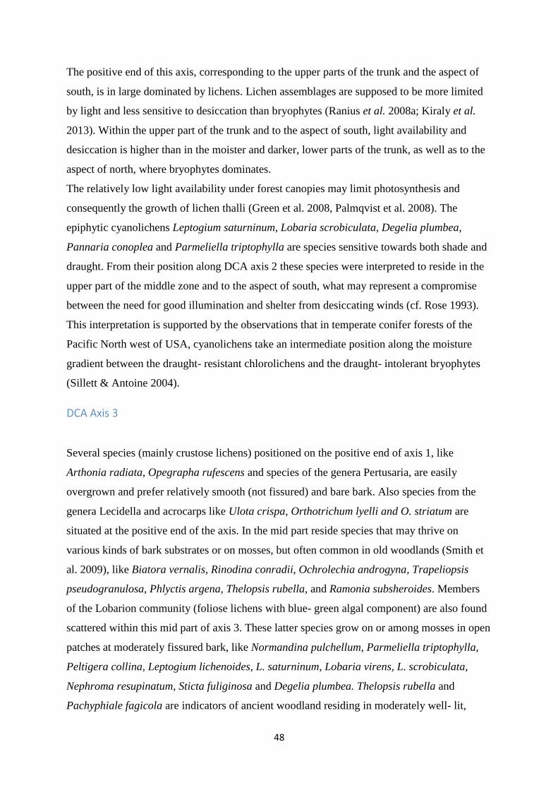
48

The positive end of this axis, corresponding to the upper parts of the trunk and the aspect of

south, is in large dominated by lichens. Lichen assemblages are supposed to be more limited

by light and less sensitive to desiccation than bryophytes (Ranius et al. 2008a; Kiraly et al.

2013). Within the upper part of the trunk and to the aspect of south, light availability and

desiccation is higher than in the moister and darker, lower parts of the trunk, as well as to the

aspect of north, where bryophytes dominates.

The relatively low light availability under forest canopies may limit photosynthesis and

consequently the growth of lichen thalli (Green et al. 2008, Palmqvist et al. 2008). The

epiphytic cyanolichens Leptogium saturninum, Lobaria scrobiculata, Degelia plumbea,

Pannaria conoplea and Parmeliella triptophylla are species sensitive towards both shade and

draught. From their position along DCA axis 2 these species were interpreted to reside in the

upper part of the middle zone and to the aspect of south, what may represent a compromise

between the need for good illumination and shelter from desiccating winds (cf. Rose 1993).

This interpretation is supported by the observations that in temperate conifer forests of the

Pacific North west of USA, cyanolichens take an intermediate position along the moisture

gradient between the draught- resistant chlorolichens and the draught- intolerant bryophytes

(Sillett & Antoine 2004).

DCA Axis 3

Several species (mainly crustose lichens) positioned on the positive end of axis 1, like

Arthonia radiata, Opegrapha rufescens and species of the genera Pertusaria, are easily

overgrown and prefer relatively smooth (not fissured) and bare bark. Also species from the

genera Lecidella and acrocarps like Ulota crispa, Orthotrichum lyelli and O. striatum are

situated at the positive end of the axis. In the mid part reside species that may thrive on

various kinds of bark substrates or on mosses, but often common in old woodlands (Smith et

al. 2009), like Biatora vernalis, Rinodina conradii, Ochrolechia androgyna, Trapeliopsis

pseudogranulosa, Phlyctis argena, Thelopsis rubella, and Ramonia subsheroides. Members

of the Lobarion community (foliose lichens with blue- green algal component) are also found

scattered within this mid part of axis 3. These latter species grow on or among mosses in open

patches at moderately fissured bark, like Normandina pulchellum, Parmeliella triptophylla,

Peltigera collina, Leptogium lichenoides, L. saturninum, Lobaria virens, L. scrobiculata,

Nephroma resupinatum, Sticta fuliginosa and Degelia plumbea. Thelopsis rubella and

Pachyphiale fagicola are indicators of ancient woodland residing in moderately well- lit,

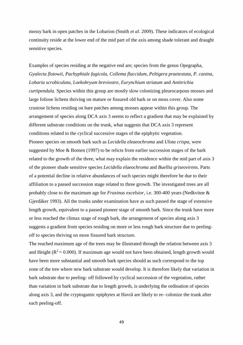
49

mossy bark in open patches in the Lobarion (Smith et al. 2009). These indicators of ecological

continuity reside at the lower end of the mid part of the axis among shade tolerant and draught

sensitive species.

Examples of species residing at the negative end are; species from the genus Opegrapha,

Gyalecta flotowii, Pachyphiale fagicola, Collema flaccidum, Peltigera praetextata, P. canina,

Lobaria scrobiculata, Loekobryum breviostre, Eurynchium striatum and Antitrichia

curtipendula. Species within this group are mostly slow colonizing pleurocarpous mosses and

large foliose lichens thriving on mature or fissured old bark or on moss cover. Also some

crustose lichens residing on bare patches among mosses appear within this group. The

arrangement of species along DCA axis 3 seems to reflect a gradient that may be explained by

different substrate conditions on the trunk, what suggests that DCA axis 3 represent

conditions related to the cyclical successive stages of the epiphytic vegetation.

Pioneer species on smooth bark such as Lecidella eleaeochroma and Ulota crispa, were

suggested by Moe & Botnen (1997) to be relicts from earlier succession stages of the bark

related to the growth of the three, what may explain the residence within the mid part of axis 3

of the pioneer shade sensitive species Lecidella elaeochroma and Buellia griseovirens. Parts

of a potential decline in relative abundances of such species might therefore be due to their

affiliation to a passed succession stage related to three growth. The investigated trees are all

probably close to the maximum age for Fraxinus excelsior, i.e. 300-400 years (Nedkvitne &

Gjerdåker 1993). All the trunks under examination have as such passed the stage of extensive

length growth, equivalent to a passed pioneer stage of smooth bark. Since the trunk have more

or less reached the climax stage of rough bark, the arrangement of species along axis 3

suggests a gradient from species residing on more or less rough bark structure due to peeling-

off to species thriving on more fissured bark structure.

The reached maximum age of the trees may be illustrated through the relation between axis 3

and Height (R2 = 0.000). If maximum age would not have been obtained, length growth would

have been more substantial and smooth bark species should as such correspond to the top

zone of the tree where new bark substrate would develop. It is therefore likely that variation in

bark substrate due to peeling- off followed by cyclical succession of the vegetation, rather

than variation in bark substrate due to length growth, is underlying the ordination of species

along axis 3, and the cryptogamic epiphytes at Havrå are likely to re- colonize the trunk after

each peeling-off.

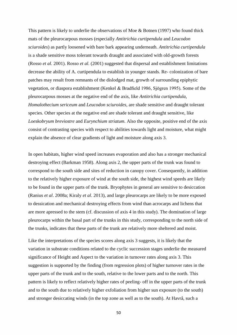
50

This pattern is likely to underlie the observations of Moe & Botnen (1997) who found thick

mats of the pleurocarpous mosses (especially Antitrichia curtipendula and Leucodon

sciuroides) as partly loosened with bare bark appearing underneath. Antitrichia curtipendula

is a shade sensitive moss tolerant towards draught and associated with old-growth forests

(Rosso et al. 2001). Rosso et al. (2001) suggested that dispersal and establishment limitations

decrease the ability of A. curtipendula to establish in younger stands. Re- colonization of bare

patches may result from remnants of the dislodged mat, growth of surrounding epiphytic

vegetation, or diaspora establishment (Kenkel & Bradfield 1986, Sjögren 1995). Some of the

pleurocarpous mosses at the negative end of the axis, like Antitrichia curtipendula,

Homalothecium sericeum and Leucodon sciuroides, are shade sensitive and draught tolerant

species. Other species at the negative end are shade tolerant and draught sensitive, like

Loeskobryum breviostre and Eurynchium striatum. Also the opposite, positive end of the axis

consist of contrasting species with respect to abilities towards light and moisture, what might

explain the absence of clear gradients of light and moisture along axis 3.

In open habitats, higher wind speed increases evaporation and also has a stronger mechanical

destroying effect (Barkman 1958). Along axis 2, the upper parts of the trunk was found to

correspond to the south side and sites of reduction in canopy cover. Consequently, in addition

to the relatively higher exposure of wind at the south side, the highest wind speeds are likely

to be found in the upper parts of the trunk. Bryophytes in general are sensitive to desiccation

(Ranius et al. 2008a; Kiraly et al. 2013), and large pleurocarps are likely to be more exposed

to dessication and mechanical destroying effects from wind than acrocarps and lichens that

are more apressed to the stem (cf. discussion of axis 4 in this study). The domination of large

pleurocarps within the basal part of the trunks in this study, corresponding to the north side of

the trunks, indicates that these parts of the trunk are relatively more sheltered and moist.

Like the interpretations of the species scores along axis 3 suggests, it is likely that the

variation in substrate conditions related to the cyclic succession stages underlie the measured

significance of Height and Aspect to the variation in turnover rates along axis 3. This

suggestion is supported by the finding (from regression plots) of higher turnover rates in the

upper parts of the trunk and to the south, relative to the lower parts and to the north. This

pattern is likely to reflect relatively higher rates of peeling- off in the upper parts of the trunk

and to the south due to relatively higher exfoliation from higher sun exposure (to the south)

and stronger desiccating winds (in the top zone as well as to the south). At Havrå, such a

51

pattern is highly plausible due to the position of the trunks in a south- facing slope at the south

side of Sørfjorden, where the south side of the trunk therefore is relatively higher exposed

than the north side both to irradiation as well as to winds.

DCA Axis 4

At the positive, upper end of axis 4 reside Frullania fragilifolia, species of the genera

Orthotrichum, Leidella elaeochroma, and Parmelia sulcata. These species are sensitive

towards shade and resistant towards draught. Also the shade tolerant and draught tolerant

Opegrapha rufescens and Phlyctis argena are found in the upper part. The above mentioned

species are more or less strongly pressed against the substrate, reside within the upper parts of

the trunk in environments with little retention of water and exposed to more or less irradiation

depending on the degree of stem inclination.

Species with different abilities towards light and moisture, and belonging to the groups of

liverworts, small foliose lichens and small pleurocarps, are positioned within the mid part of

the axis. The most abundant of these species are Metzgeria furcata, Leucodon sciuroides,

Homalothecium sericeum, Hypnum cupressiforme, species of the genera Lepraria, Isothecium

myosuroides, Leptogium lichenoides and Melanelixia subaurifera. These species are found

either within the middle zone of the trunk or scattered throughout the entire trunk. Some

variation in environments of light and moisture exist between the upper mid part and the

lower mid part of the trunk (cf. discussion of DCA axis 2), but relative to the heterogeneity

throughout the entire trunk, the environmental heterogeneity within the mid part can be

characterized as low. Consequently, species residing in the mid part do not vary extensively

with respect to their moderate to high resistance towards shade and draught. This

homogeneity in species abilities towards light and moisture is reflected through the species’

moderate adherence to substrate, corresponding to a lack of highly pendulate pleurocarps,

most crustose lichens (except for the leprose) and large foliose lichens.

In the negative end of axis 4, Nephroma resupinatum, Peltigera resupinatum, Bazzania

tricrenata, Loeskobryum breviostre and Thuidium tamariscinum reside. These latter species

are all sensitive towards draught, more or less tolerant towards shade and found in the basal

part of the trunk on the slanting upper side. The most striking common feature unifying these

latter species is however the way they are loosely pressed to their substrate, indicating a

52

residence within moist and shady environments. Evaporation is likely to vary both with height

on the stem as well as with inclination within each height (cf. discussion of axis 2 in appendix

1). A gradient of stem inclination is consequently related to the way species are adapted to

shade and moisture stress. Axis 4 seem therefore to reflect variation in the degree to which

species adhere to their substrate.

Appendix 4. Importance of Height, Aspect and Management

The results from the model testing show that there are very small probabilities of that the

variation in temporal turnover along DCA axis 2 as function of Height would have occurred

by chance if the null hypothesis was true. The large F- value for axis 2 (F = 4.44) of the

Anova- test of the regression of turnover rates along axis 2 as function of Height provide

evidence to reject the null hypothesis of no variation in rates along this axis (no beta

diversity). The significance of Height to turnover rates along axis 2 indicate an important role

to gradients in light and moisture to the vertical distribution of the epiphytes along the stem.

The interaction term between Height and Aspect was not significant for axis 2, indicating that

the change in temporal turnover rate by moving from one level to the next (e.g. from middle

to top) of the predictor of Height does not depend on the predictor of Aspect, and vice versa.

The null model (intercept-only model) represented the most parsimonious model for axis 2.

These results indicate that the model with Height does not have predictive power to the

variation in temporal turnover rates along axis 2. The fact that the null model is provided with

the greatest support does only signify that it is the best model out of the ones included in the

selection, and that the potential variation in temporal turnover rates cannot be predicted by the

variables in the alternative hypotheses. There may be variation that is unrelated to the

measured gradient, like indicated through the large F- value.

The results from the model testing show that there are very small probabilities of that the

variation in temporal turnover along DCA axis 2 as function of Aspect would have occurred

by chance if the null hypothesis was true. The large F- value for axis 2 (F = 3.52) of the

Anova- test of the regression of turnover rates along axis 2 as function of Aspect provide

evidence to reject the null hypothesis of no variation in rates along this axis.

Aspect and Height was significant to variation in temporal turnover along DCA axis 3. The

results from the regressions show that it is unlikely that variation as function of these

53

variables would have occurred by chance if the null hypothesis was true. The large F- values

for axis 3 (F = 3.27 for Aspect and F = 15.8 for Height) from the Anova- tests of these

regressions provide evidence to reject the null hypotheses of no variation in rates along this

axis (no beta diversity).

The interaction term between Height and Aspect was not significant for axis 3, indicating that

the change in temporal turnover rate by moving from one level to the next (e.g. from middle

to top) of the predictor of Height does not depend on the predictor of Aspect, and vice versa.

The model with Height as the only fixed effect factor represented the most parsimonious

model for axis 3. These results indicate that Height has predictive power to the variation in

temporal turnover rates along axis 3, whereas Aspect does not have predictive power. Other

relevant factors that were not measured and included as potential predictive variables

obviously might have had higher predictive power than Height to the variation along axis 3.