Template for for the Jurnal Teknologi · Jurnal Teknologi Full Paper ... 1) minimum number of ......

75:10 (2015) 97–110 | www.jurnalteknologi.utm.my | eISSN 2180–3722 |

Jurnal

Teknologi

Full Paper

INVESTIGATION OF DATUM CONSTRAINTS EFFECT

IN TERRESTRIAL LASER SCANNER SELF-

CALIBRATION

Mohd Azwan Abbasa, Halim Setanb, Zulkepli Majidb, Albert

K. Chongc, Lau Chong Luhb, Khairulnizam M. Idrisb, Mohd

Farid Mohd Ariffb

aFaculty of Architecture, Planning & Surveying, Universiti

Teknologi MARA, 02600 Arau, Perlis, Malaysia bFaculty of Geoinformation & Real Estate, Universiti

Teknologi Malaysia, 81310 UTM Johor Bahru, Johor,

Malaysia cSchool of Civil Engineering & Surveying, University of

Southern Queensland, Australia

Article history

Received

6 April 2015

Received in revised form

12 August 2015

Accepted

23 August 2015

*Corresponding author

[email protected]

Graphical abstract

Abstract The ability to provide rapid and dense three-dimensional (3D) data have made many 3D

applications easier. However, similar to other optical and electronic instruments, data from TLS can

also be impaired with errors. Self-calibration is a method available to investigate those errors in TLS

observations which has been adopted from photogrammetry technique. Though, the network

configuration applied by both TLS and photogrammetry techniques are quite different. Thus,

further investigation is required to verify whether the photogrammetry principal regarding datum

constraints selection is applicable to TLS self-calibration. To ensure that the assessment is thoroughly

done, the datum constraints analyses were carried out using three variant network configurations:

1) minimum number of scan stations, 2) minimum number of surfaces for targets distribution, and

3) minimum number of point targets. Via graphical and statistical, the analyses of datum

constraints selection have indicated that the parameter correlations obtained are significantly

similar.

Keywords: Terrestrial laser scannesr, self-calibration, network configuration, datum constraints

Abstrak Kemampuan untuk memberikan data tiga-dimensi (3D) dengan cepat dan padat telah

menyebabkan banyak aplikasi 3D menjadi lebih mudah. Walau bagaimanapun, sama seperti

peralatan optik dan elektronik yang lain, data TLS juga dipengaruhi dengan selisih. Kalibrasi-sendiri

ialah kaedah yang wujud untuk menyiasat selisih tersebut bagi cerapan TLS yang mana telah

diadaptasi dari teknik fotogrammetri. Tetapi, konfigurasi jaringan yang digunapakai oleh TLS dan

fotogrammetri agak berbeza. Maka, siasatan lanjut diperlukan bagi memastikan samada prinsip

fotogrammetri berkenaan pemilihan kekangan datum boleh digunapakai untuk kalibrasi-sendiri

TLS. Bagi memastikan penilaian dibuat secara teliti, analisis kekangan datum dilaksanakan dengan

tiga konfigurasi jaringan yang berbeza: 1) bilangan minimum bagi stesen cerapan, 2) bilangan

minimum permukaan bagi meletakkan target, dan 3) bilangan minimum target. Secara grafik dan

statistik, analisis pemilihan kekangan datum menunjukkan bahawa korelasi parameter yang

diperoleh adalah signifikan sama.

Kata kunci: Terrestrial laser scanner,kalibrasi-senidiri, konfigurasi jaringan, kekangan datum

© 2015 Penerbit UTM Press. All rights reserved

TLS Self-Calibration

Photogrammetry Self-

Calibration

98 Mohd Azwan Abbas et al. / Jurnal Teknologi (Sciences & Engineering) 75:10 (2015) 97–110

1.0 INTRODUCTION

Capability of terrestrial laser scanner (TLS) in three-

dimensional (3D) data acquisition is not questionable,

with rapid and high resolution 3D data provided, TLS

has become an option for numerous applications

(e.g. cultural heritage, facility management,

architecture and 3D city modeling). Recently, TLS has

also been utilised for accurate measurements which

require millimetre geometric accuracy including

landslide monitoring [1-2], structural deformation

measurement [3-4], dam monitoring [5], automobile

dimensioning [6] and highway clearance

measurement [7], among others.

However, similar as others electronic and optical

instruments, the impairing of errors in the observed

data have been major causes that reduced the

quality of TLS data. According to Lichti [8], there are

seventeen systematic errors can be modeled in each

TLS observations (e.g. range, horizontal direction and

vertical angle). For quality assurance, these

systematic errors have to be investigated and

modelled, and subsequently applied to the raw data

to improve the accuracy. There are two approaches

available to investigate these errors, either separately

(component calibration) or simultaneously (system

calibration).

Figure 1 Facilities and devices required for component

calibration, (a) Calibration trackline, (b) Targets with slots,

and (c) Calibration baseline [9,10]

Due to the difficulty to provide the requirements of

special laboratories and tools to performed

component calibration (Figure 1), it is only

implemented by academician and manufacturers. It

is applicable to investigate systematic errors but most

of the component calibration is used to identify the

best-suited applications of the calibrated TLS and also

to compare the performance of TLS from different

manufacturers. In contrast, system calibration requires

a room with appropriate targets to determine all

significant systematic errors (Figure 5). Considering the

most convenience procedure to the TLS users, system

calibration which can be implemented through self-

calibration was selected to investigate the systematic

errors in this study.

Self-calibration used to perform system calibration

was originally adapted from photogrammetry

approach. Thus, similar to the photogrammetry self-

calibration, the datum constraints applied for TLS self-

calibration can be defined as follows: (1) minimum;

and (2) inner constraints. However, according to

Reshetyuk [11] both datum constraints (used in

photogrammetry calibration) have their own

limitations. The use of minimum constraints tends to

cause large correlation between object points and

some of the calibration parameters. For the inner

constraints, it has unfavourable property of increasing

the correlations between the calibration and exterior

orientation parameters.

Analysis of correlations in self-calibration usually

performed to investigate the quality of the

adjustment. Though, in TLS self-calibration, the analysis

focuses to reduce the correlations between

calibration parameters and other system parameters.

There are several causes of parameters correlation: (1)

weak network geometry; and (2) the type of

constraint used. Lichti [8] has reported the analysis of

correlations which has indicated high correlations

between calibration parameters and exterior

orientation parameters as well as object points. Author

assumes that weak network geometry (e.g. limitation

size of calibration field and distribution of range) was

the reason for that finding. With the objective to

investigate the effect of constraint selection in

parameters correlation for TLS self-calibration, this

study will focus on the later causes.

Although self-calibration approach was adapted

from photogrammetry, requirement for network

configurations (e.g. targets distribution, calibration

field and positions of the sensor) for the self-calibration

for both TLS [8] and photogrammetry [12] are quite

different. As illustrated in the Figure 2,

photogrammetry self-calibration only require

appropriate calibration frame with fairly distributed

targets. Camera positions will be based on this frame

with strong convergence [12].

Figure 2 Photogrammetry self-calibration using

Photomodeler V5.0 software

While the network configuration for TLS self-

calibration has been addressed by Lichti [8] as follows:

i. A large variety of ranges is needed to

accurately estimate the ranging error terms,

in particular the rangefinder offset;

ii. A large range of elevation angle

measurements is necessary to recover some

of the angular measurement error model

coefficients;

(a) (b) (c)


iii. The self-calibration can be conducted from

a minimum of two separate instrument

locations provided that they have

orthogonal orientation in the horizontal plane

( angles, rotation about Z axis); and

iv. The calibration quality, as measured by

reduced parameter correlations, is

proportional to the number of targets used.

This argument regarding network configuration has

initially indicate that the principal of datum constraints

for photogrammetry is not relevant for TLS self-

calibration. However, further investigation in necessity

to statistically verify the effect of datum constraints to

TLS self-calibration. With the intention to scrutinise this

issue, this study has performed self-calibration for a

Faro Photon 120 scanner. Both datum constraints were

used to carry out bundle adjustment and results were

statistically analysed to determine whether there is

any significant difference in correlation between the

calculated parameters. Furthermore, to ensure this

study has critically evaluated this issue, different

network configurations were adopted during

experiments. Three elements were taking into account

during network configurations as follows: (1) the

minimum number of scan stations; (2) the minimum

number of surfaces on which targets are distributed;

and (3) the minimum number of point targets. As a

result, analyses of datum constraints were carried out

based on full networks and minimum networks

configuration according to the previous three

elements.

2.0 GEOMETRICAL MODEL FOR SELF-

CALIBRATION

Due to the very limited knowledge regarding the inner

functioning of modern terrestrial laser scanners, most

researchers have made assumptions about a suitable

error model for TLS based on errors involved in

reflectorless total stations [8]. Since the data

measured by TLS are range, horizontal and vertical

angle, the equations for each measurement are

augmented with systematic error correction model as

follows [11]:

rzyxr,Range 222 (1)

Horizontal direction,

y

xtan 1

(2)

Vertical angle,

22

1

yx

ztan (3)

Where,

x, y, z = Cartesian coordinates of point in scanner

space.

Δr, Δφ, Δθ = Systematic error model for range,

horizontal angle and vertical angle, respectively.

Since this study was conducted on panoramic

scanners (Faro Photon 120), the angular observations

computed using equation (2) and equation (3) must

be modified. This is due to the scanning procedure

applied by panoramic scanner, which rotates only

through 180° to provide 360° information for horizontal

and vertical angles as depicted in Figure 3.

Figure 3 Angular observation ranges for (a) Hybrid scanner

and (b) Panoramic scanner

Based on Lichti [13], the modified mathematical

model for a panoramic scanner can be presented as

follows:

180

y

xtan 1

(4)

22

1

yx

ztan180

(5)

The modified models above, equation (4) and

equation (5) are only applicable when horizontal

angle is more than 180° as shown in Figure 3.

Otherwise, equation (2) and equation (3) will be used,

which means that panoramic scanner has two

equations for both angular observations.

Regarding the systematic errors model, this study

has employed the most significant errors model as

applied by Reshetyuk [11] as follows:

i. Systematic error model for range.

0ar (6)

ii. Systematic error model for horizontal angle.

tanbsecb 10 (7)

Where,

b0 = Collimation axis error

b1 = Trunnion axis error

iii. Systematic error model for vertical angle.

0c (8)

Lichti et al. [14] mentioned that systematic error

models for panoramic scanner can be recognised

based on the trends in the residuals from a least

squares adjustment that excludes the relevant

calibration parameters. In most cases, the trend of un-


modelled systematic error closely resembles the

analytical form of the corresponding correction

model. Figure 4 shows the trend of the adjustment

residuals for systematic error model.

Based on Figure 4, all systematic error models are

identified by plotting a graph of adjusted observations

against residuals. The graph of adjusted range against

its residuals (Figure 4a) will indicate a constant range

error (a0) if the trends appear like an incline line. When

residuals of the horizontal observations are plotted

against the adjusted vertical angles a trend like the

secant function, mean that the scanner has significant

collimation axis error (Figure 4b). Trunnion axis error

can be identified by having a trend like tangent

function as shown in Figure 4c. For vertical index error,

by plotting a graph of adjusted horizontal angles

against vertical angles residual, this systematic error

model is considered exist when the trend looks like the

big curve as depicted in Figure 4d.

Figure 4 Systematic errors for terrestrial laser scanner, (a) Un-

modelled constant error, a0, (b) Collimation axis error, b0, (c)

Trunnion axis error, b1 and (d) Vertical circle index error, c0

In order to perform self-calibration bundle

adjustment, the captured x, y, z of the laser scanner

observations need to be expressed as functions of the

position and orientation of the laser scanner in a

global coordinate system [15]. Based on rigid-body

transformation, for the jth target scanned from the ith

scanner station, the equation is as follows:

)TZ(R)TY(R)TX(Rz

)TZ(R)TY(R)TX(Ry

)TZ(R)TY(R)TX(Rx

Zij33Yij23Xij13i

Zij32Yij22Xij12i

Zij31Yij21Xij11i

(9)

Where,

iii zyx = Coordinates of the target in the

scanner coordinate system

33R = Components of rotation matrix between the

two coordinate systems for the ith scanner station

jjj ZYX = Coordinates of the jth target in the

global coordinate system

ZiYiXi TTT = Coordinates of the ith scanner

station in the global coordinate system.

3.0 DATUM CONSTRAINTS

Terrestrial laser scanner data involves 3D network, thus,

theoretically seven datum constraints are required to

remove datum defects. However, with the range

observation, the scale is defined implicitly, which

means that scanner network only requires six datum

constraints.

To employ minimum constraints, all six datum need

to be fixed. There are several procedures available to

implement minimum constraints:

i. According to Reshetyuk [11], six fix

coordinates distributed over 3 non-collinear

points are required in order to use minimum

constraints; or

ii. As applied by Gielsdorf et al. [16], position

and orientation of one scanner station which

represent by exterior orientation parameters

were fixed to employ minimum constraints.

In order to use the minimum constraints, this study

has fixed the exterior orientation parameters for the

first scanner station. Based on the original shape of

design matrix A as shown in equation (10) and

equation (11), the process of removing matrix element

for minimum constraints can be expressed as follows:

(10)

Where,

n = number of observations

u = number of unknown parameters

AEO = Design matrix for exterior orientation (EO)

parameters

ACP = Design matrix for calibration parameters (CP)

AOP = Design matrix for object points (OP)

New design matrix A without EO parameters for first

scanner station is in the form:

nOPnCPnEO

2OP2CP2EO

1OP1CP

un

AAA0

AA0A

AA00

A

(11)

Removed

OPCPEOun AAAA

nOPnCPnEO

2OP2CP2EO

1OP1CP1EO

AAA00

AA0A0

AA00A


Application of the inner constraints for this study has

been adopted from Lichti [8]. The constraint imposed

on object points (OP) to remove the datum defects

are given in matrix form as:

0

X̂

X̂

X̂

.G00

OP

CP

EO

T

o

(12)

Where,

EOX̂ = Vector of the exterior orientation parameters

CPX̂ = Vector of the calibration parameters

OPX̂ = Vector of the object points

The true form of the datum design constraint matrix

oG is as follows [14].

(13)

The bordered system of normal equation follows from

the standard parametric least square is given as:

N X̂ + U = 0

0

0

0

PLA

k

X̂

X̂

X̂

0G

GPAA T

c

OP

CP

EO

o

T

o

T

(14)

Where,

A = Design matrix

P = Weight matrix

L = Observations matrix

kc = Vector of Lagrange multipliers

4.0 EXPERIMENTAL

In this study, a self-calibration was performed for the

Faro Photon 120 panoramic terrestrial laser scanner.

The calibration was carried out in a laboratory with

dimensions 15.5m (length) x 9m (width) x 3m (height).

The full network configurations were adopted based

on Lichti [8] conditions to ensure the quality of the

obtained results.

i. The 138 black and white targets were well-

distributed on the four walls and ceiling

(Figure 5); and

Figure 5 Self-calibration for the Faro Photo 120

scanner

ii. Seven scan stations were used to observe the

targets. As shown in Figure 6, five scan stations

were located at the each corner and centre

of the room. The other two were positioned

close to the two corners with the scanner

orientation manually rotated 90° from

scanner orientation at the same corner. In all

cases the height of the scanner was placed

midway between the floor and the ceiling.

Figure 6 Scanner locations during self-calibration

With the aid of the Faroscene V5.0 software, all

measured targets were extracted except for those

that have high incidence angle which are not able to

be recognised. A self-calibration bundle adjustment

was performed using both datum constraints (e.g.

inner and minimum constraints) with precision settings

based on the manufacturer’s specification, which

were 2mm for distance and 0.009º for both angle

measurements. After two iterations, the bundle

adjustment process converged.

To perform datum constraints analyses, values of

correlation coefficient were extracted from variance

covariance matrix using the following formula [17]:

0XY

X0Z

YZ0

100

010

001

0XY

X0Z

YZ0

100

010

001

0XY

X0Z

YZ0

100

010

001

G

nn

nn

nn

22

22

22

11

11

11

To


yx

xyxy

(15)

Where,

ji xx : Covariance between parameters.

ix : Standard deviation of the parameter.

Correlations analyses were carried out between the

calibration parameters and other system parameters

(e.g. exterior orientation parameters and object

points). To assess the significant difference in datum

constraints selection, several graphs were plotted to

visualise the difference between the parameter

correlations of inner and minimum constraints.

Furthermore, statistical analysis was performed to

evaluate the results obtained from the plotted graphs.

The F-variance ratio test was used to investigate the

significance of the difference between two

populations [18]. The null hypothesis, H0, of the test is

that the two population variances are not significantly

different while the alternate hypothesis is that they are

different. The F-variance ratio test is defined as:

2

2

2

1F

(16)

Where, 2

1 : Variance of population 1.

The null hypothesis is rejected if the calculated F

value is higher than the critical F value (from the F-

distribution table) at the 5% significance level. The

rejection of H0 shows that the test parameters are not

equal. If the test shows no significant difference, then

both datum constraints are suitable for the self-

calibration bundle adjustment for terrestrial laser

scanner.

With intention to investigate the concrete evidence

of the effect of datum constraints selection, this study

has employed several variations of network

configurations as follows:

i. Full network configurations using 138 targets,

all surfaces (e.g. four walls and a ceiling) and

7 scan stations.

ii. Minimum number of scan stations.

iii. Minimum number of surfaces.

iv. Minimum number of targets with seventy

percent reduction.

Configuration of full network is already discussed at

the earlier paragraph of this section. For the second

configuration, number of scan stations was reduced

from seven scan stations (Figure 6) one by one until

two scan stations left as shown in Figure 7. For each

time when the number of scan station reduced, the

self-calibration bundle adjustment is performed and

the datum constraints analyses were carried out.

Results obtained will indicate any significant effect of

datum constraints selection with variation of scan

stations.

Figure 7 Reducing number of scan stations.

The subsequent configuration focuses on reducing

the numbers of surfaces used for target distribution.

This is very crucial due to the difficulty to get surfaces

similar as laboratory condition for on-site application.

In laboratory, all targets can be distributed to all walls,

a ceiling and a floor but for on-site situation,

sometimes there are only two walls and a floor

available. In this study, four walls and a ceiling were

used to distribute all 138 targets. From these five

surfaces, experiment is carry out by removing those

surfaces on by one until two surfaces left as shown in

Figure 8. For each removing procedure, self-

calibration bundle adjustment will be performed and

followed with datum constraints analyses.


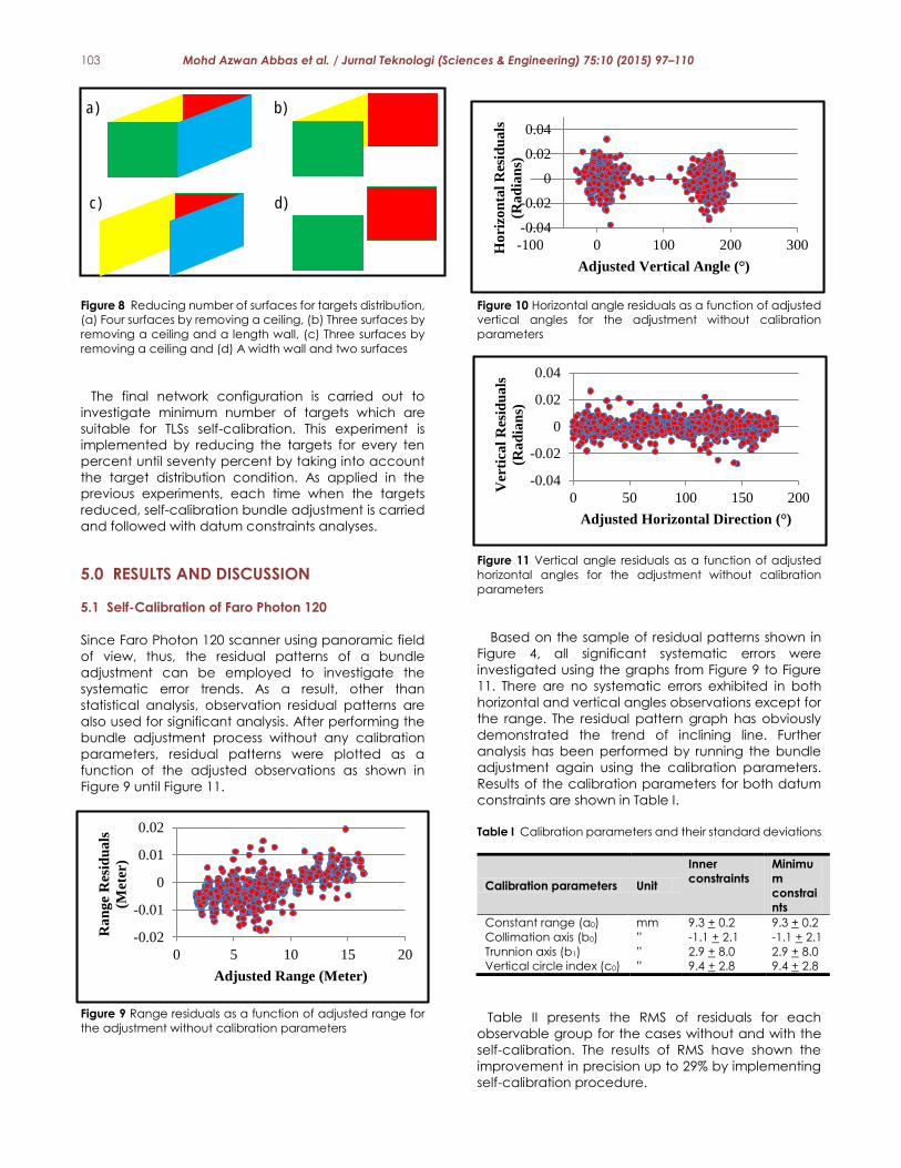
Figure 8 Reducing number of surfaces for targets distribution,

(a) Four surfaces by removing a ceiling, (b) Three surfaces by

removing a ceiling and a length wall, (c) Three surfaces by

removing a ceiling and (d) A width wall and two surfaces

The final network configuration is carried out to

investigate minimum number of targets which are

suitable for TLSs self-calibration. This experiment is

implemented by reducing the targets for every ten

percent until seventy percent by taking into account

the target distribution condition. As applied in the

previous experiments, each time when the targets

reduced, self-calibration bundle adjustment is carried

and followed with datum constraints analyses.

5.0 RESULTS AND DISCUSSION

5.1 Self-Calibration of Faro Photon 120

Since Faro Photon 120 scanner using panoramic field

of view, thus, the residual patterns of a bundle

adjustment can be employed to investigate the

systematic error trends. As a result, other than

statistical analysis, observation residual patterns are

also used for significant analysis. After performing the

bundle adjustment process without any calibration

parameters, residual patterns were plotted as a

function of the adjusted observations as shown in

Figure 9 until Figure 11.

Figure 9 Range residuals as a function of adjusted range for

the adjustment without calibration parameters

Figure 10 Horizontal angle residuals as a function of adjusted

vertical angles for the adjustment without calibration

parameters

Figure 11 Vertical angle residuals as a function of adjusted

horizontal angles for the adjustment without calibration

parameters

Based on the sample of residual patterns shown in

Figure 4, all significant systematic errors were

investigated using the graphs from Figure 9 to Figure

11. There are no systematic errors exhibited in both

horizontal and vertical angles observations except for

the range. The residual pattern graph has obviously

demonstrated the trend of inclining line. Further

analysis has been performed by running the bundle

adjustment again using the calibration parameters.

Results of the calibration parameters for both datum

constraints are shown in Table I.

Table I Calibration parameters and their standard deviations

Calibration parameters Unit

Inner

constraints

Minimu

m

constrai

nts

Constant range (a0) mm 9.3 + 0.2 9.3 + 0.2

Collimation axis (b0) ” -1.1 + 2.1 -1.1 + 2.1

Trunnion axis (b1) ” 2.9 + 8.0 2.9 + 8.0

Vertical circle index (c0) ” 9.4 + 2.8 9.4 + 2.8

Table II presents the RMS of residuals for each

observable group for the cases without and with the

self-calibration. The results of RMS have shown the

improvement in precision up to 29% by implementing

self-calibration procedure.

a) b)

c) d) -0.04

-0.02

0

0.02

0.04

-100 0 100 200 300Ho

rizo

nta

l R

esid

ua

ls

(Ra

dia

ns)

Adjusted Vertical Angle (°)

-0.04

-0.02

0

0.02

0.04

0 50 100 150 200V

erti

cal

Res

idu

als

(Ra

dia

ns)

Adjusted Horizontal Direction (°)

-0.02

-0.01

0

0.01

0.02

0 5 10 15 20

Ra

ng

e R

esid

ua

ls

(Met

er)

Adjusted Range (Meter)


Table II RMS of residuals from the adjustments without and

with calibration parameters

Observable RMS

(without)

RMS

(with)

Improvement

in

percentage

Range 5.6mm 4.0mm 29%

Horizontal

direction 41.0” 37.1” 10%

Vertical angle 24.0” 22.4” 7%

In order to have a concrete solution regarding the

significant of the estimated systematic error model,

statistical tests were performed. All calibration

parameters were tested to investigate their significant.

The null hypothesis, H0, of the test is that the parameter

is not significant, otherwise the hypothesis indicate

that parameter is significant. Using 95% confidence

level, the results of the test are shown in Table III.

Table III Significant test for calibration parameters

parameters

According to Table III, the null hypothesis was

accepted when the calculated (Calc.) ‘t’ is smaller

than critical ‘t’ and vice versa. The results obtained

show that null hypothesis was rejected for parameter

of constant rangefinder offset (a0), and vertical circle

index (c0) parameters. This indicates that those

parameters are significant. For the collimation axis (b0)

and trunnion axis (b1) errors, the null hypothesis has

been accepted.

5.2 Datum Constraints Analyses

As discussed in Section 1, one of the causes of

parameters correlation is the type of constraints used.

Furthermore, Reshetyuk [11] did mention that selection

of datum constraints can results different types of

parameters correlation in photogrammetry

application. Thus, investigation is carried to ensure

whether that principal is applicable for TLS self-

calibration. Through graphical and statistical analysis,

the results obtained are discussed in detail.

Below are the plotted graphs (Figure 12 until Figure

16) illustrated the comparison of parameters

correlation between inner and minimum constraints.

Due to the large number of parameters involved (e.g.

seven scan stations, four calibration parameters and

138 targets) in variance covariance matrix, then this

study has used mean values.

Figure 12 Parameter correlations of constant range and

exterior orientation parameters (full network configuration)

Figure 13 Parameter correlations of collimation axis and


Figure 14 Parameter correlations of trunnion axis and exterior

orientation parameters (full network configuration)

Number of scanner stations 7

Degree of freedom 1925

Critical value for ‘t’ (95%) 1.645

Calibration parameters Calc. ‘t’ Significant Test

Constant range ( 0a ) 46.5 Significant

Collimation axis ( 0b ) 0.524 Not Significant

Trunnion axis ( 1b ) 0.363 Not Significant

Vertical circle index ( 0c ) 3.357 Significant


Figure 15 Parameter correlations of vertical circle index and


Figure 16 Parameter correlations of calibration parameters

and object points (full network configuration)

Figure 12 to Figure 15 represent the plotted

correlation between four calibration parameters (e.g.

constant range, collimation axis, trunnion axis and

vertical circle index) and exterior orientation (EO)

parameters (e.g. omega, phi, kappa, translation X,

translation Y and translation Z). While Figure 16 is

illustrate the correlation of calibration parameters and

object points. In each figure, correlations of both

datum constraints are attached for visually examine

the difference. However, initial conclusion can be

made that there are no significant differences

between datum constraints as well as the values of

correlations are consider small with maximum number

is 0.58 (between vertical circle index and phi in Figure

15). Through statistical analysis, F-variance ratio test

has mathematically proved the similarity of results

obtained.

Table IV F-variance ratio test for full network configuration

Parameter

Correlations

Calculated F >/< Critical F

a0 / EO 0.09 < 5.05

b0 / EO 0.42 < 5.05

b1 / EO 0.01 < 5.05

c0 / EO 0.69 < 5.05

CP / OP 0.01 < 9.28

Table IV shows that in all cases, with 95% confidence

level, the calculated F is smaller than critical F, which

indicates the acceptation of null hypothesis (H0). Since

this is the results of full network which have employed

very strong network geometry, thus, the good findings

is expected.

With intention to investigate the robust conclusion

regarding similarity of the correlation results yielded

from both datum constraints, this study has carried out

similar analysis for different type of network

configurations. The first configuration is by reducing

the number of scan stations. For each stations

configuration, statistical analysis is performed as

depicted in Table V.

Table V F-variance ratio test for different stations

configurations

Configuratio

n

Parameter

Correlation

s

Calculate

d F

>/

<

Critica

l F

6 Stations

a0 / EO 0.07 < 5.05

b0 / EO 0.18 < 5.05

b1 / EO 0.16 < 5.05

c0 / EO 0.71 < 5.05

CP / OP 0.86 < 9.28

5 Stations

a0 / EO 0.05 < 5.05

b0 / EO 0.37 < 5.05

b1 / EO 0.00 < 5.05

c0 / EO 0.63 < 5.05

CP / OP 0.86 < 9.28

4 Stations

a0 / EO 0.17 < 5.05

b0 / EO 0.32 < 5.05

b1 / EO 0.21 < 5.05

c0 / EO 0.77 < 5.05

CP / OP 0.75 < 9.28

3 Stations

a0 / EO 0.06 < 5.05

b0 / EO 0.00 < 5.05

b1 / EO 1.63 < 5.05

c0 / EO 0.47 < 5.05

CP / OP 0.19 < 9.28

2 Stations

a0 / EO 0.14 < 5.05

b0 / EO 0.11 < 5.05

b1 / EO 0.15 < 5.05

c0 / EO 0.15 < 5.05

CP / OP 0.11 < 9.28

For all cases, the null hypothesis are accepted

which mean no significant difference between both

datum constraints. Furthermore, Figure 17 until Figure

21 have visualised the similarity of the results (e.g.

parameters correlation) obtained from both datum

constraints for the case of minimum number of scan

station (e.g. two scan stations). Additionally, the trend

of the plotted graphs are quiet similar to the full

network configurations.



exterior orientation parameters (minimum stations

configuration)



configuration)


orientation parameters (minimum stations configuration)



configuration)


and object points (minimum stations configuration)

Through different surfaces configurations

experiment, the datum constraints analysis was again

performed. Outcomes of F-variance ratio test were

organised in the Table VI for four different types of

surfaces configurations. Values of calculated F for all

circumstances have indicated the acceptance of null

hypothesis, which also has increase the certainty of

previous conclusion, there is no significant effect in

datum constraints selection. Moreover, the minimum

configuration for surfaces using two walls as illustrated

in Figure 22 to Figure 26 does not indicated any

obvious different between inner and minimum

constraints, the graphs as well have similar trends as

full network configuration.


Table VI F-variance ratio test for different surfaces

configurations

Configuratio

n

Parameter

Correlation

s

Calculate

d F

>/

<

Critica

l F

4 Walls

a0 / EO 0.01 < 5.05

b0 / EO 0.25 < 5.05

b1 / EO 3.18 < 5.05

c0 / EO 0.61 < 5.05

CP / OP 0.69 < 9.28

2 Walls and a

Ceiling

a0 / EO 0.01 < 5.05

b0 / EO 0.26 < 5.05

b1 / EO 1.60 < 5.05

c0 / EO 0.56 < 5.05

CP / OP 0.31 < 9.28

3 Walls

a0 / EO 0.00 < 5.05

b0 / EO 0.50 < 5.05

b1 / EO 0.81 < 5.05

c0 / EO 0.63 < 5.05

CP / OP 0.40 < 9.28

2 Walls

a0 / EO 0.00 < 5.05

b0 / EO 0.07 < 5.05

b1 / EO 0.40 < 5.05

c0 / EO 0.40 < 5.05

CP / OP 0.02 < 9.28


exterior orientation parameters (minimum surfaces

configuration)



configuration)


orientation parameters (minimum surfaces configuration)



configuration)


and object points (minimum surfaces configuration)

For the final configuration, different number of

targets distribution, F-variance ratio test has

concretely proved that there is no significant effect in

parameter correlations from the datum constraints

selection. As shown in Table VII, the null hypotheses

have again statistically verified the significant similarity

of both datum constraints. In addition, the trend

depicted in Figure 27 to Figure 31 for minimum number

of targets (e.g. 70% reduction or equivalent to 41

targets) have a similar shape as full network

configuration.


Table VII F-variance ratio test for different targets

configurations

Configuratio

n

Parameter

Correlation

s

Calculate

d F

>/

<

Critica

l F

10% Targets

Reduction

a0 / EO 0.07 < 5.05

b0 / EO 0.20 < 5.05

b1 / EO 0.53 < 5.05

c0 / EO 0.61 < 5.05

CP / OP 0.52 < 9.28

20% Targets

Reduction

a0 / EO 0.08 < 5.05

b0 / EO 0.27 < 5.05

b1 / EO 0.27 < 5.05

c0 / EO 0.61 < 5.05

CP / OP 0.45 < 9.28

30% Targets

Reduction

a0 / EO 0.10 < 5.05

b0 / EO 0.39 < 5.05

b1 / EO 0.29 < 5.05

c0 / EO 0.62 < 5.05

CP / OP 0.61 < 9.28

40% Targets

Reduction

a0 / EO 0.09 < 5.05

b0 / EO 0.28 < 5.05

b1 / EO 0.52 < 5.05

c0 / EO 0.56 < 5.05

CP / OP 0.58 < 9.28

50% Targets

Reduction

a0 / EO 0.09 < 5.05

b0 / EO 0.27 < 5.05

b1 / EO 1.22 < 5.05

c0 / EO 0.55 < 5.05

CP / OP 0.30 < 9.28

60% Targets

Reduction

a0 / EO 0.08 < 5.05

b0 / EO 0.18 < 5.05

b1 / EO 0.61 < 5.05

c0 / EO 0.56 < 5.05

CP / OP 0.27 < 9.28

70% Targets

Reduction

a0 / EO 0.10 < 5.05

b0 / EO 0.14 < 5.05

b1 / EO 0.01 < 5.05

c0 / EO 0.71 < 5.05

CP / OP 0.30 < 9.28


exterior orientation parameters (minimum targets

configuration)



configuration)


orientation parameters (minimum targets configuration)



configuration)



and object points (minimum targets configuration)

As discussed in Section 1, according to

photogrammetry self-calibration, the used of inner

constraints can increase the correlations between the

calibration parameters and exterior orientations.

Otherwise, employing minimum constraints tends to

cause large correlations between object points and

calibration parameters. However, trend in the graphs

plotted (e.g. for full network, minimum stations,

minimum surfaces and minimum targets

configurations) indicates different assumption.

Surprisingly, for all plotted graphs, the comparisons

between the parameter correlations obtained from

using both datum constraints are quite similar. Since

the only causes for parameter correlation are network

geometry and selection of datum constraints, thus,

the outcomes of this study has graphically and

statistically proved that the later cause is not relevant

for TLS self-calibration. However, the network

geometry should be made carefully, this is very crucial

to ensure the quality of the results obtained (e.g.

calibration parameters as well as to de-correlate the

parameters).

6.0 CONCLUSION

A self-calibration procedure used for TLS calibration

was originally adapted from photogrammetry

technique, however the photogrammetry network

configuration is not suitable for TLS application. This is

due to the observables and measurement technique

implemented by both photogrammetry and TLS are

different. Therefore, further investigation was carried

out to evaluate whether similar effect in datum

constraints selection for photogrammetry is relevant

for TLS. Graphical and statistical analyses were

employed to examine any significant differences in

the parameter correlations obtained from inner or

minimum constraints. To ensure that the investigation

is thoroughly executed, the datum constraints

analyses were carried out using three variant network

configurations: 1) minimum number of scan stations, 2)

minimum number of surfaces for targets distribution,

and 3) minimum number of point targets. The datum

constraints analyses for all network configurations

have indicated that the selection of datum constraints

does not affect the values of parameter correlations.

Both inner and minimum constraints can provide

significantly similar parameter correlations.

Nevertheless, the network configuration is a very

crucial procedure to ensure that the correlation

between the calculated parameters can be

reduced.

Acknowledgement

The present research was made possible through a

Vote 00G23 under UTM research grant GUP Flagship

by Universiti Teknologi Malaysia (UTM). Special thanks

goes to Ministry of Higher Education (MoHE) and

Photogrammetry & Laser Scanning Research Group,

INFOCOMM Research Alliance, UTM for the facility

and technical support in this project.

References [1] Syahmi, M. Z., Wan Aziz, W. A., Zulkarnaini, M. A., Anuar, A.

and Othman, Z. 2011. The Movement Detection on the

Landslide Surface by Using Terrestrial Laser Scanning.

Control and System Graduate Research Colloquium

(ICSGRC), 2011 IEEE, Shah Alam, Selangor.

[2] Wan Aziz, W. A., Khairul, N. T. and Anuar. 2012. A. Slope

Gradient Analysis at Different Resolution Using Terrestrial

Laser Scanner. Signal Processing and its Applications

(CSPA), 2012 IEEE 8th International Colloquium, Melaka.

[3] Gordon, S. J. and Lichti, D. D. 2007. Modeling Terrestrial

Laser Scanner Data for Precise Structural Deformation

Measurement. ASCE Journal of Surveying Engineering. 133

(2): 72-80.

[4] Rönnholm, P., Nuikka, M., Suominen, A., Salo, P., Hyyppä,

H., Pöntinen, P., Haggrén, H., Vermeer, M., Puttonen, J., Hirsi,

H., Kukko, A., Kaartinen, H., Hyyppä, J. and Jaakkola. 2009.

A. Comparison of Measurement Techniques and Static

Theory Applied to Concrete Beam Deformation. The

Photogrammetric Record. 24(128): 351-371.

[5] González-Aguilera, D. Gómez-Lahoz, J., Sánchez, J. 2008. A

New Approach for Structural Monitoring of Large Dams

With a Three-dimensional Laser Scanner. Sensors. 8(9): 5866-

5883.

[6] González-Jorge, H., Riveiro, B., Arias, P., and Armesto, J.

2012. Photogrammetry and Laser Scanner Technology

Applied to Length Measurements in Car Testing

Laboratories. Measurement. 45: 354-363.

[7] Riveiro, B., González-Jorge H., Varela, M., and Jauregui, D.

V., 2013. Validation of Terrestrial Laser Scanning and

Photogrammetry Techniques For The Measurement Of

Vertical Underclearance And Beam Geometry In Structural

Inspection Of Bridges. Measurement. (46): 184-794.

[8] Lichti, D. D. 2007. Error Modelling, Calibration and Analysis

of an AM-CW Terrestrial Laser Scanner System. ISPRS Journal

of Photogrammetry & Remote Sensing. 61: 307-324.

[9] Brian, F., Catherine, L. C. and Robert, R. 2004. Investigation

on Laser Scanners. IWAA2004, 2004 CERN, Geneva.

[10] Mohd Azwan, A., Halim, S., Zulkepli, M., Albert K. C.,

Khairulnizam, M. I. and Anuar, A. 2013. Calibration and

Accuracy Assessment of Leica ScanStation C10 Terrestrial

Laser Scanner. Development in Multidimensional Spatial

Data Models, Springer Lecture Notes in Geoinformation

and Cartography (LNG&C), March 2013. 33-47.

[11] Reshetyuk, Y. 2009. Self-Calibration and Direct

Georeferencing in Terrestrial Laser Scanning. Doctoral


Thesis in Infrastructure, Royal Institute of Technology (KTH),

Stockholm, Sweden, 2009.

[12] Fraser, C. S. 1996. Network Design. In Close

Photogrammetry and Machine Vision. Edited by K. B.

Atkinson. Whittles Publishing, Roseleigh House,

Latheronwheel, Scotland, UK. 256-279.

[13] Lichti, D. D. 2010. A Review of Geometric Models and Self-Calibration Methods for Terrestrial Laser Scanner. Bol. Ciȇnc.

Geod., sec. Artigos, Curitiba. 3-19.

[14] Lichti, D. D., Chow, J. and Lahamy, H. 2011. Parameter De-

Correlation and Model-Identification in Hybrid-Style

Terrestrial Laser Scanner Self-Calibration. ISPRS Journal of

Photogrammetry and Remote Sensing. 66: 317-326.

[15] Schneider, D. 2009. Calibration of Riegl LMS-Z420i based on

a Multi-Station Adjustment and a Geometric Model with

Additional Parameters. The International Archives of the

Photogrammetry, Remote Sensing and Spatial Information

Sciences. 38 (Part 3/W8): 177-182.

[16] Gielsdorf, F., Rietdorf, A. and Gruendig, L. 2004. A Concept

for the Calibration of Terrestrial Laser Scanners. TS26

Positioning and Measurement Technologies and Practices

II-Laser Scanning and Photogrammetry. FIG Working Week

2004, Athens, Greece. 1-10.

[17] Abdul, W. I. and Halim, S. 2001. Pelarasan Ukur. Kuala

Lumpur: Dewan Bahasa dan Pustaka. 5-9.

[18] Gopal, K. K. 1999. 100 Statistical Test. Thousand Oaks,

California: SAGE Publications Ltd. 37-38.

Template for for the Jurnal Teknologi · Jurnal Teknologi Full Paper ... 1) minimum number of ......

Documents

Transcript of Template for for the Jurnal Teknologi · Jurnal Teknologi Full Paper ... 1) minimum number of ......