Service Engineering

QED Q's Quality & Efficiency Driven Telephone Call/Contact Centers

Service Engineering

QED Q's Quality & Efficiency Driven Telephone Call/Contact Centers

INFORMS San-Francisco November 15, 2005

e.mail : avim@tx.technion.ac.il

Website: http://ie.technion.ac.il/serveng

Contents

1. Background: Service Engineering, Call Centers, WFM

2. Operational Regime: Quality-Driven, Efficiency-Driven

QED Q's = Quality & Efficiency Driven

in an M/M/N (Erlang-C) world

3. Intuition; Dimensioning

Contents

1. Background: Service Engineering, Call Centers, WFM

2. Operational Regime: Quality-Driven, Efficiency-Driven

QED Q's = Quality & Efficiency Driven

in an M/M/N (Erlang-C) world

3. Intuition; Dimensioning

Leading to models, inference and tools:

)A-Erlang (Customers) Abandoning( Impatient. 4

5. Predictably (Time) Varying Queues

Contents

1. Background: Service Engineering, Call Centers, WFM

2. Operational Regime: Quality-Driven, Efficiency-Driven

QED Q's = Quality & Efficiency Driven

in an M/M/N (Erlang-C) world

3. Intuition; Dimensioning

Leading to models, inference and tools:

)A-Erlang (Customers) Abandoning( Impatient. 4

5. Predictably (Time) Varying Queues

6. General Service Times (M/D/N, M/LN/N, …)

7. Human/Smart Customers and Smart Systems

8. Heterogeneous Customer Types and

Partially Overlapping Server Skills (SBR)

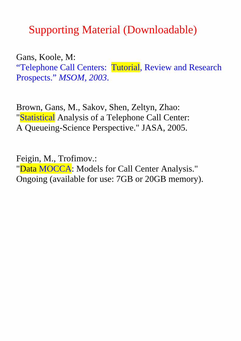
Supporting Material (Downloadable) Gans, Koole, M:

, Review and Research Tutorial: Telephone Call Centers“Prospects.” MSOM, 2003.

Brown, Gans, M., Sakov, Shen, Zeltyn, Zhao:

: Analysis of a Telephone Call Center Statistical" A Queueing-Science Perspective." JASA, 2005.

Feigin, M., Trofimov.:

." r Analysis CenteModels for Call: MOCCAData " Ongoing (available for use: 7GB or 20GB memory).

Research-Partners

QED/QD/ED Q's:

)A-Erlang(Patience -M+N/M/M: arnett, ReimanG

patience-G+N/M/M: Zeltyn

support-D, finite=G/ N w/G/G: Jelelnkovic, Momcilovic

G +N/G/G: Kaspi, Ramanan

Service Networks: Rider, Stolyar, Massey, Reiman

Dimensioning:

C and A -Erlang: Borst, Reiman; Zeltyn

V - and Reversed-V: Gurvich,Armony

: hitt; Jennings, Feldman, RozenshmidtMassey, W

Stablizing Time-Varying Q's SBR:

Control : ; StolyarAtar, Reiman

Controllability-Null: Atar, Shaikhet

History

by Basharin et al, " ,Markov. A. ALife of Work of The "

Linear Algebra and its Applications, 2004.

:)C / B(Erlang Models Solutions of Some Problems in the Theory of . "K.Erlang, A

Probabilities of Significance in Automatic Telephone Exchanges", Elektroteknikeren, 1917; English translation in the "Life and Work of A.K. Erlang" 1948, by Brokemeyer et al.

:Dimensioning / Root Staffing-Square

On the Rational Determination of the : ".K.Erlang, ANumber of Circuits", 1924; first published in the "Life…," 1948; proofs on page 120-6.

:)Irritation / A-Erlang(Impatient Customers

, Ericsson Technics, "Etude des Delais D'Attente ".Palm, C1937. Palm, C.: "Methods of Judging the Annoyance Caused by Congestion", Tele, 1953.

Tele-Nets: Call/Contact Centers Scope Examples

Information (uni, bi-dir)

#411, Tele-pay, Help Desks

Business Tele-Banks, #800-Retail

Emergency Police #911

Mixed Info + Emerg. Info + Bus.

Utility, City Halls Airlines, Insurance, Cellular

Scale

– 10s to 1000s of agents in a “single” Call Center – X% of work force in call centers (up to several millions) – 70% of total business transactions in call centers – 20% growth rate of the call center industry – Leading-edge technology, but 70% costs for “people”

Trends: THE interface for/with customers

– Contact Centers (E-Commerce/Multimedia), outsourcing,… – Retails outlets of 21-Century – but also the Sweat-shops of the 21-Century

Erlang-C = M/M/N

arrivals queueACD

agents

Rough Performance Analysis

Peak 10:00 – 10:30 a.m., with 100 agents

400 calls

3:45 minutes average service time

2 seconds ASA (Average Speed of Answer)

Rough Performance Analysis

Peak 10:00 – 10:30 a.m., with 100 agents

400 calls

3:45 minutes average service time

2 seconds ASA

Offered load R = λ × E(S)

= 400 × 3:45 = 1500 min./30 min.

= 50 Erlangs

Occupancy ρ = R/N

= 50/100 = 50%

Rough Performance Analysis

Peak 10:00 – 10:30 a.m., with 100 agents

400 calls

3:45 minutes average service time

2 seconds ASA

Offered load R = λ × E(S)

= 400 × 3:45 = 1500 min./30 min.

= 50 Erlangs

Occupancy ρ = R/N

= 50/100 = 50%

⇒ Quality-Driven Operation (Light-Traffic)

⇒ Classical Queueing Theory (M/G/N approximations)

Above: R = 50, N = R + 50, ≈ all served immediately.

Rule of Thumb: N = ⎡ ⎤R R δ+ , 0>δ service-grade.

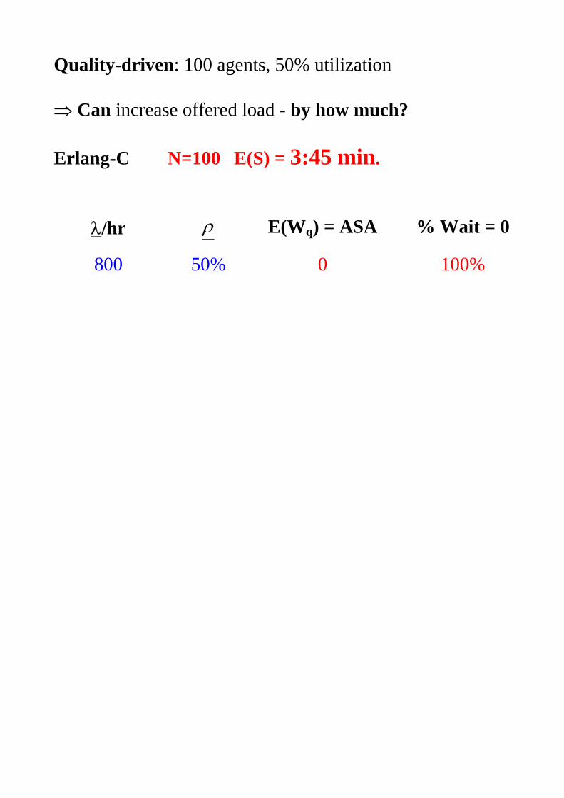
Quality-driven: 100 agents, 50% utilization

⇒ Can increase offered load - by how much?

Erlang-C N=100 E(S) = 3:45 min.

λ/hr ρ E(Wq) = ASA % Wait = 0

800 50% 0 100%

Quality-driven: 100 agents, 50% utilization

⇒ Can increase offered load - by how much?

Erlang-C N=100 E(S) = 3:45 min.

λ/hr ρ E(Wq) = ASA % Wait = 0

800 50% 0 100%

1400 87.5% 0:02 min. 88%

1550 96.9% 0:48 min. 35%

1580 98.8% 2:34 min. 15%

1585 99.1% 3:34 min. 12%

Quality-driven: 100 agents, 50% utilization

⇒ Can increase offered load - by how much?

Erlang-C N=100 E(S) = 3:45 min.

λ/hr ρ E(Wq) = ASA % Wait = 0

800 50% 0 100%

1400 87.5% 0:02 min. 88%

1550 96.9% 0:48 min. 35%

1580 98.8% 2:34 min. 15%

1585 99.1% 3:34 min. 12%

⇒ Efficiency-driven Operation (Heavy Traffic)

)()(1

10| SESEN

WWWN

Nqqq →⋅

−⋅=>≈

ρρ = 3:45 !

1,1)1( →=− NNN ρρ

Above: R = 99, N = R + 1, ≈ all delayed. Rule of Thumb: N = ⎡ ⎤γ+ R , 0>γ service grade.

Changing N (Staffing) in Erlang-C

E(S) = 3:45

λ/hr N OCC ASA % Wait = 0

1585 100 99.1% 3:34 12%

Changing N (Staffing) in Erlang-C

E(S) = 3:45

λ/hr N OCC ASA % Wait = 0

1585 100 99.1% 3:34 12%

1599 100 99.9% 59:33 0%

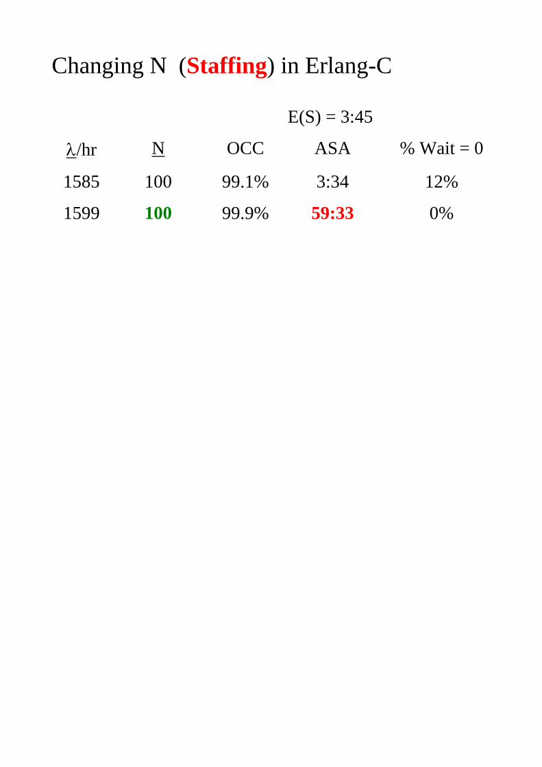
Changing N (Staffing) in Erlang-C

E(S) = 3:45

λ/hr N OCC ASA % Wait = 0

1585 100 99.1% 3:34 12%

1599 100 99.9% 59:33 0%

1599 100+1 98.9% 3:06 13%

1599 102 98.0% 1:24 24%

1599 105 95.2% 0:23 50%

Changing N (Staffing) in Erlang-C

E(S) = 3:45

λ/hr N OCC ASA % Wait = 0

1585 100 99.1% 3:34 12%

1599 100 99.9% 59:33 0%

1599 100+1 98.9% 3:06 13%

1599 102 98.0% 1:24 24%

1599 105 95.2% 0:23 50%

⇒ New Rationalized Operation

Efficiently driven, in the sense that OCC > 95%;

Quality-Driven, 50% answered immediately

QED Regime = Quality- and Efficiency-Driven Regime

Economies of Scale in a Frictionless Environment Above: R = 100, N = R + 5, 50% delayed.

⋅ Safety-Staffing N = ⎡R + β R ⎤ , β > 0 .

QED Theorem (Halfin-Whitt, 1981)

Consider a sequence of M/M/N models, N=1,2,3,…

Then the following 3 points of view are equivalent:

• Customer NN

Plim∞→

{Wait > 0} = α , 0 < α < 1;

• Server βρ =−∞→

)1(lim NN

N , 0 < β < ∞ ;

• Manager , ×= λR E(S) large; RRN β+≈

Here 1

)(1

−

⎥⎦

⎤⎢⎣

⎡−

+=β

βαh

,

where is the hazard-rate of standard-normal. )(⋅h

Extremes:

Everyone waits: 01 =⇔= βα Efficiency-driven

No one waits: ∞=⇔= βα 0 Quality-driven

1

⋅ Safety-Staffing: Performance

R = ×λ E(S) Offered load (Erlangs)

N = R + 321Rβ β = “service-grade” > 0

= R + ∆ ⋅ safety-staffing

Expected Performance:

% Delayed 0,)(-

)1)P(1

>⎥⎦

⎤⎢⎣

⎡+=≈

−

ββ

ββh

Erlang-C

Congestion index = E∆

=⎥⎦

⎤⎢⎣

⎡>

10WaitE(S)

Wait ASA

% ⎭⎬⎫

⎩⎨⎧

>> 0WaitT(S)E

Wait ∆= T-e TSF

Servers’ Utilization = N

1NR β

−≈ Occupancy

2

19

The Halfin-Whitt Delay Function P( )

Beta

Alpha

M/M/N (Erlang-C) with Many Servers: N ↑ ∞

Q Q+

0

1

N-1

N

2

N+1

Q(0) = N : all servers busy, no queue.

Recall E2,N =

[1 +

TN−1,N

TN,N−1

]−1

=

[1 +

1− ρN

ρNE1,N−1

]−1

.

Here TN−1,N =1

λNE1,N−1∼ 1

Nµ× h(−β)/√

N∼ 1/µ

h(−β)√

N

which applies as√

N (1− ρN) → β, −∞ < β < ∞.

Also TN,N−1 =1

Nµ(1− ρN)∼ 1/µ

β√

N

which applies as above, but for 0 < β < ∞.

Hence, E2,N ∼[1 +

β

h(−β)

]−1

, assuming β > 0.

QED: N ∼ R + β√

R for some β, 0 < β < ∞⇔ λN ∼ µN − βµ

√N

⇔ ρN ∼ 1− β√N

, namely limN→∞

√N (1− ρN) = β.

Theorem (Halfin-Whitt, 1981) QED ⇔ limN→∞

E2,N =[1 + β

h(−β)

]−1.

6

Approximating Queueing and Waiting

• QN = {QN(t), t ≥ 0} : QN(t) = number in system at t ≥ 0.

• Q̂N = {Q̂N(t), t ≥ 0} : stochastic process obtained by

centering and rescaling:

Q̂N =QN −N√

N

• Q̂N(∞) : stationary distribution of Q̂N

• Q̂ = {Q̂(t), t ≥ 0} : process defined by: Q̂N(t)d→ Q̂(t).

?-

-

-

? ?

Q̂N(t) Q̂N(∞)

Q̂(t) Q(∞)

t →∞

t →∞

N →∞ N →∞

Approximating (Virtual) Waiting Time

V̂N =√

N VN ⇒ V̂ =

[1

µQ̂

]+

(Puhalskii, 1994)

9

Economics: Quality vs. Efficiency

Dimensioning: with Borst and Reiman

Quality D(t) delay cost (t = delay time)

Efficiency C(N) staffing cost (N = # agents) Optimization: N* minimizes Total Costs

• C >> D : Efficiency-driven • C << D : Quality-driven • C D : Rationalized - QED ≈

Framework: Asymptotic theory, M/M/N, N ∞↑

Economics: ⋅ Safety-Staffing Costs: d = delay/waiting

c = staffing

Min Total Costs

Asymptotically Optimal

N* ≈ R + y*⎟⎠⎞

⎜⎝⎛

cd R

Here y*(r) ≈ ( )21

121

/

/rr

⎟⎠

⎞⎜⎝

⎛−+ π

, 0 < r < 10

≈ 21

2ln 2

/r⎟⎠⎞

⎜⎝⎛

π , r large.

22

Square-Root Safety Staffing: RryRN )(*+= r = cost of delay / cost of staffing

23

⋅ Safety-Staffing: Overview

Simple Rule-of-thumb: N* ≈ R + y*⎟⎠⎞

⎜⎝⎛

cd R

Robust: covers also efficiency- and quality-driven Accurate: to within 1 agent (from few to many 100’s) typically

Relevant: Medium to Large CC do perform as above.

Instructive: In large call centers, high resource utilization and

service levels could coexist, which is enabled by economies of scale

that dominate stochastic variability.

Example: 100 calls per minute, at 4 min. per call

⇒ R = 400, least number of agents

20RR

** y)r(y=≈

∆ , with y*: 0.5–1.5 ;

Safety staffing: 2.5%–7.5% of R=Min ! ⇒ “Real” Problem?

Performance: N* % wait > 20 sec. Utilization

400 + 11 20% 97%

400 + 29 1% 93%

�

�

�

�

Arrivals: Inhomogeneous Poisson

Figure 1: Arrivals (to queue or service) – “Regular” Calls

0

20

40

60

80

100

120

Calls/Hr (Reg)

7 8 9 10 11 12 13 14 15 16 17 18 19 20 21 22 23 24

VRU Exit Time

1030

�

�

�

�

Figure 12: Mean Service Time (Regular) vs. Time-of-day (95% CI) (n =

42613)

Time of Day

Mea

n S

ervi

ce T

ime

10 15 20

100

120

140

160

180

200

220

240

7 8 9 10 11 12 13 14 15 16 17 18 19 20 21 22 23 24

3029

31

Service Time

Survival curve, by Types

Time

Surv

ival

Means (In Seconds)

NW (New) = 111

PS (Regular) = 181

NE (Stocks) = 269

IN (Internet) = 381

32

14

33

Beyond Data Averages

Short Service Times

AVG:200

STD:249

AVG: 185

STD: 238

7.2 %?

Jan – Oct:

Log-NormalAVG: 200

STD: 249

Nov – Dec:

45

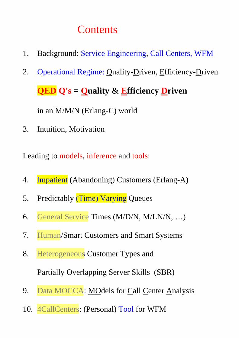
Contents

1. Background: Service Engineering, Call Centers, WFM

2. Operational Regime: Quality-Driven, Efficiency-Driven

QED Q's = Quality & Efficiency Driven

in an M/M/N (Erlang-C) world

3. Intuition, Motivation

Leading to models, inference and tools:

)A-Erlang (Customers) Abandoning( Impatient. 4

5. Predictably (Time) Varying Queues

6. General Service Times (M/D/N, M/LN/N, …)

7. Human/Smart Customers and Smart Systems

8. Heterogeneous Customer Types and

Partially Overlapping Server Skills (SBR)

9. Data MOCCA: MOdels for Call Center Analysis

10. 4CallCenters: (Personal) Tool for WFM

Erlang-A (with G-Patience): M/M/N+G

lost calls

arrivals

lost calls

abandonment

busy

FRONT

queue

ACD

QED Theorem (Garnett, M. and Reiman '02; Zeltyn '03)

Consider a sequence of M/M/N+G models, N=1,2,3,…

Then the following points of view are equivalent:

• QED %{Wait > 0} ≈ α , 0 < α < 1 ;

• Customers %{Abandon} ≈ Nγ , 0 < γ ;

• Agents OCC Nγβ +

−≈ 1 −∞ < β < ∞ ;

• Managers RRN β+≈ , ×= λR E(S) not small;

QED performance (ASA, ...) is easily computable, all in terms

of β (the square-root safety staffing level) – see later.

Covers also the Extremes:

α = 1 : N = R - γ R Efficiency-driven

α = 0 : N = R + γ R Quality-driven

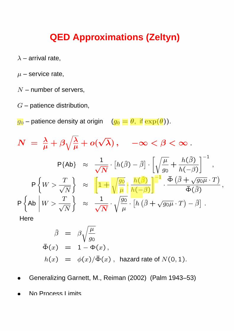
QED Approximations (Zeltyn)

λ – arrival rate,

µ – service rate,

N – number of servers,

G – patience distribution,

g0 – patience density at origin (g0 = θ, if exp(θ)).

N = λµ + β

√λµ + o(

√λ) , −∞ < β < ∞ .

P{Ab} ≈ 1√N

· [h(β̂) − β̂] ·

[õ

g0+

h(β̂)

h(−β)

]−1

,

P

{W >

T√N

}≈

[1 +

√g0

µ· h(β̂)

h(−β)

]−1

· Φ̄(β̂ +

√g0µ · T )

Φ̄(β̂),

P

{Ab

∣∣∣∣ W >T√N

}≈ 1√

N·√

g0

µ· [h (

β̂ +√

g0µ · T ) − β̂]

.

Here

β̂ = β

õ

g0

Φ̄(x) = 1 − Φ(x) ,

h(x) = φ(x)/Φ̄(x) , hazard rate of N(0,1).

• Generalizing Garnett, M., Reiman (2002) (Palm 1943–53)

• No Process Limits

HW/GMR Delay Functions

α vs. β

0

0.1

0.2

0.3

0.4

0.5

0.6

0.7

0.8

0.9

1

-3 -2.5 -2 -1.5 -1 -0.5 0 0.5 1 1.5 2 2.5 3Beta

Del

ay P

roba

bilit

y

Halfin-Whitt Garnett(0.1) Garnett(0.5) Garnett(1)Garnett(2) Garnett(5) Garnett(10) Garnett(20)Garnett(50) Garnett(100)

θ/µ

Halfin-Whitt

QED Erlang-A

Example: "Real" Call Center (The "Right Answer" for the "Wrong Reasons")

Time-Varying (two-hump) arrival functions common (Adapted from Green L., Kolesar P., Soares J. for benchmarking.)

0

500

1000

1500

2000

2500

0 1 2 3 4 5 6 7 8 9 10 11 12 13 14 15 16 17 18 19 20 21 22 23

Hour of Day

Cal

ls p

er H

ou

r

Assume: Service and abandonment times are both

Exponential, with mean 0.1 (6 min.)

Time-Varying Arrivals

Model tt NMM // + M

Parameters λ(t) µ ? θ

? Nt = Rt + tRβ

Time-Varying Arrivals

Model tt NMM // + M

Parameters λ(t) µ ? θ

? Nt = Rt + tRβ

Offered Load: ∫−

=⋅−=t

Stt duuESEStER )()()( λλ

Average # in ∞// MMt

Time-Varying Arrivals

Model tt NMM // + M

Parameters λ(t) µ ? θ

? Nt = Rt + tRβ

Offered Load: ∫−

=⋅−=t

Stt duuESEStER )()()( λλ

Average # in ∞// MMt

Gives rise to TIME-STABLE PEFORMANCE (Why? Think tt NMM // + M with µ = θ;

And if µ ≠ θ, or generally:

use the Iterative Simulation-Based Staffing Algorithm

in Feldman, M., Massey and Whitt, 2005.)

HW/GMR Delay Functions

α vs. β

0

0.1

0.2

0.3

0.4

0.5

0.6

0.7

0.8

0.9

1

-3 -2.5 -2 -1.5 -1 -0.5 0 0.5 1 1.5 2 2.5 3Beta

Del

ay P

roba

bilit

y

Halfin-Whitt Garnett(0.1) Garnett(0.5) Garnett(1)Garnett(2) Garnett(5) Garnett(10) Garnett(20)Garnett(50) Garnett(100)

θ/µ

Halfin-Whitt

QED Erlang-A

Delay Probability α Delay Probability

0

0.1

0.2

0.3

0.4

0.5

0.6

0.7

0.8

0.9

1

0 1 2 3 4 5 6 7 8 9 10 11 12 13 14 15 16 17 18 19 20 21 22 23

Target Alpha=0.1 Target Alpha=0.2 Target Alpha=0.3Target Alpha=0.4 Target Alpha=0.5 Target Alpha=0.6Target Alpha=0.7 Target Alpha=0.8 Target Alpha=0.9

Abandon ProbabilityAbandon Probability

0

0.1

0.2

0.3

0.4

0.5

0.6

0.7

0.8

0 1 2 3 4 5 6 7 8 9 10 11 12 13 14 15 16 17 18 19 20 21 22 23

Taget Alpha=0.1 Taget Alpha=0.2 Taget Alpha=0.3

Taget Alpha=0.4 Taget Alpha=0.5 Taget Alpha=0.6

Taget Alpha=0.7 Taget Alpha=0.8 Taget Alpha=0.9

Abandon Probability

0

0.02

0.04

0.06

0.08

0.1

0.12

0.14

0 1 2 3 4 5 6 7 8 9 10 11 12 13 14 15 16 17 18 19 20 21 22 23

Taget Alpha=0.1 Taget Alpha=0.2 Taget Alpha=0.3

Taget Alpha=0.4 Taget Alpha=0.5 Taget Alpha=0.6

Taget Alpha=0.7 Taget Alpha=0.8 Taget Alpha=0.9

Real Call Center: Empirical waiting time, given positive wait

(1) α=0.1 (QD) (2) α=0.5 (QED) (3) α=0.9 (ED)

The "Right Answer" (for the "Wrong Reasons")

Prevalent Practice (PSA) ⎡ ⎤)()( SEtNt ⋅= λ

"Right Answer" ttt RRN ⋅+≈ β (MOL)

)()( SEStERt ⋅−= λ

The "Right Answer" (for the "Wrong Reasons")

Prevalent Practice (PSA) ⎡ )()( SEtNt ⋅= λ ⎤

"Right Answer" ttt RRN ⋅+≈ β (MOL)

)()( SEStERt ⋅−= λ Practice ≈ "Right" β ≈ 0 (QED) and ≈ stable over service-durations )(tλ

Practice Improved ⎡ ⎤)()]([ SESEtNt ⋅−= λ

0

500

1000

1500

2000

2500

0 1 2 3 4 5 6 7 8 9 10 11 12 13 14 15 16 17 18 19 20 21 22 23

Hour of Day

Cal

ls p

er H

ou

r

QED Staffing (β=0 iff α=0.5)

0

500

1000

1500

2000

2500

0 1 2 3 4 5 6 7 8 9 10 11 12 13 14 15 16 17 18 19 20 21 22 230

50

100

150

200

250

Arrived Staffing Offered Load

The "Right Answer" (for the "Wrong Reasons")

Prevalent Practice (PSA) ⎡ )()( SEtNt ⋅= λ ⎤

"Right Answer" ttt RRN ⋅+≈ β (MOL)

)()( SEStERt ⋅−= λ Practice ≈ "Right" β ≈ 0 (QED) and )(tλ ≈ stable over service-durations

Practice Improved ⎡ ⎤)()]([ SESEtNt ⋅−= λ

When Optimal ? for moderately-patient customers:

1. Satisfization At least 50% to be serve immediately ⇔ 2. Optimization ⇔ Customer-Time = 2 x Agent-Salary

Time-Varying Arrivals: ⋅ Safety-Staffing

Model tt NMM // + M

Parameters λ(t) µ ? θ

? Nt = Rt + tRβ

Time-Varying Arrivals: ⋅ Safety-Staffing

Model tt NMM // + M

Parameters λ(t) µ ? θ

? Nt = Rt + tRβ

µ = θ : tLd= Poisson( ) tR

d≈ N(Rt, Rt), since ∞// MMt

∫−

=⋅−=t

Stt duuESEStER )()()( λλ offered load

Time-Varying Arrivals: ⋅ Safety-Staffing

Model tt NMM // + M

Parameters λ(t) µ ? θ

? Nt = Rt + tRβ

µ = θ : tLd= Poisson( ) tR

d≈ N(Rt, Rt), since ∞// MMt

∫−

=⋅−=t

Stt duuESEStER )()()( λλ offered load

Given Lt ≈ Rt + tZ R , d

Z = N(0,1)

choose Nt = Rt + tRβ

⇒ α = P(W > 0) ≈ P(Lt ≥ Nt) = P(Z ≥ β) = 1 – φ(β) t PASTA

⇒ β = φ–1 (1 – α) time-stable α ≡ P(Wt > 0) ?

Time-Varying Arrivals: ⋅ Safety-Staffing

Model tt NMM // + M

Parameters λ(t) µ ? θ

? Nt = Rt + tRβ

µ = θ : tLd= Poisson( ) tR

d≈ N(Rt, Rt), since ∞// MMt

∫−

=⋅−=t

Stt duuESEStER )()()( λλ offered load

Given Lt ≈ Rt + tZ R , d

Z = N(0,1)

choose Nt = Rt + tRβ

⇒ α = P(W > 0) ≈ P(Lt ≥ Nt) = P(Z ≥ β) = 1 – φ(β) t PASTA

⇒ β = φ–1 (1 – α) time-stable α ≡ P(Wt > 0) ?

Indeed, but in fact TIME-STABLE PERFORMANCE

Time-Varying Arrivals: ⋅ Safety-Staffing

Model tt NMM // + M

Parameters λ(t) µ ? θ

? Nt = Rt + tRβ

µ = θ : tLd= Poisson( ) tR

d≈ N(Rt, Rt), since ∞// MMt

∫−

=⋅−=t

Stt duuESEStER )()()( λλ offered load

Given Lt ≈ Rt + tZ R , d

Z = N(0,1)

choose Nt = Rt + tRβ

⇒ α = P(W > 0) ≈ P(Lt ≥ Nt) = P(Z ≥ β) = 1 – φ(β) t PASTA

⇒ β = φ–1 (1 – α) time-stable α ≡ P(Wt > 0) ?

Indeed, but in fact TIME-STABLE PERFORMANCE

(µ ≠ θ, or generally : Iterative Simulation-Based Algorithm)