The Pennsylvania State University

The Graduate School

College of Engineering

TECHNIQUES FOR DETERMINING THE RANGE AND

MOTION OF UHF RFID TAGS

A Thesis in

Electrical Engineering

by

Urmila Pujare

2010 Urmila Pujare

Submitted in Partial Fulfillment

of the Requirements

for the Degree of

Master of Science

December 2010

ii

The thesis of Urmila Pujare was reviewed and approved* by the following:

Raj Mittra

Professor of Electrical Engineering

Thesis Advisor

Sven Bilén

Associate Professor of Engineering Design, Electrical Engineering, and

Aerospace Engineering

Committee Member

Kenneth Jenkins

Professor of Electrical Engineering

Department Head of the Electrical Engineering

*Signatures are on file in the Graduate School

iii

Abstract

The study focuses on determining the range, velocity, and direction of motion of one or more UHF RFID-

tagged objects present within a broadcast-and-receive range of an RFID tag reader using the Phase-

Difference-of-Arrival concept. Different processing techniques with their respective advantages and

disadvantages are presented. The data, which were collected in different environmental settings and

situations, were processed and the results analyzed. In addition, the study includes an assessment of the

accuracies of the algorithms and develops theoretical methods to validate the observations. Sources of

errors were identified and suggestions regarding possible solutions and future improvements are offered.

The thesis also presents real-life application scenarios each of which uses this feature in its RFID system.

iv

TABLE OF CONTENTS

LIST OF FIGURES ................................................................................................................................... vi

LIST OF TABLES ..................................................................................................................................... ix

ACKNOWLEDGMENTS .......................................................................................................................... x

Chapter 1 Introduction .............................................................................................................................. 1

1.1 Contributions of this work ............................................................................................................... 1

1.2 Organization of the thesis ................................................................................................................ 2

1.3 Overview of the RFID system ......................................................................................................... 2

1.4 Techniques to determine RFID tag range and motion ..................................................................... 4

1.4.1 Phase Difference of Arrival ...................................................................................................... 5

1.5 Determining phase using an RFID reader ........................................................................................ 6

1.6 Mathematical introduction to tag range estimation .......................................................................... 8

Chapter 2 Tag Range Estimation Techniques ........................................................................................ 11

2.1 Processing method 1: End-point regression and linear regression ................................................. 11

2.2 Processing method 2: Periodic functional fit ................................................................................. 17

2.3 Further algorithmic details ............................................................................................................. 20

2.3.1 Phase unwrapping ................................................................................................................... 20

2.3.2 Number of phase reads, frequency spacing, and processing time ........................................... 20

2.4 Factors that contribute to errors ..................................................................................................... 21

2.4.1 Hardware errors....................................................................................................................... 21

2.4.2 Error due to signal to noise ..................................................................................................... 23

2.4.3 Dispersion due to receiver path filters or antenna characteristics ........................................... 23

2.4.4 Multipath response .................................................................................................................. 23

Chapter 3 Collection and Analysis of Tag Range Data in Different Environments ........................... 26

3.1 Anechoic chamber ......................................................................................................................... 26

3.1.1 Observations ........................................................................................................................... 29

3.2 Open field....................................................................................................................................... 30

3.2.1 Path loss theory and ground-reflection model ........................................................................ 32

3.2.2 Data collection and results ...................................................................................................... 34

3.2.3 Observations ........................................................................................................................... 47

3.3 Industrial setting ............................................................................................................................. 48

3.3.1 Observations ........................................................................................................................... 50

Chapter 4 Tag Motion/Velocity and Direction Estimation ................................................................... 52

v

4.1 Mathematical introduction to tag range estimation ........................................................................ 52

4.2 Processing method: End-point regression and linear regression .................................................... 53

4.3 Further algorithmic details ............................................................................................................. 57

4.3.1 Phase unwrapping ................................................................................................................... 57

4.3.2 Number of phase reads, time spacing, and processing time .................................................... 60

4.4 Factors that contribute to errors ..................................................................................................... 60

4.5 Data collection in industrial setting and analysis ........................................................................... 60

4.5.1 Situation-1 ............................................................................................................................... 61

4.5.2 Situation-2 ............................................................................................................................... 63

4.6 Alternate processing method for velocity and direction estimation: Kalman filtering .................. 66

4.6.1 Kalman filter theory ................................................................................................................ 66

4.6.2 Application of the discrete Kalman filter to tag velocity and direction estimation ................ 68

4.6.3 Application of the discrete Kalman filter to a real-life use ..................................................... 73

Chapter 5 Summary and Future Work .................................................................................................. 80

5.1 Applications ................................................................................................................................... 82

REFERENCES .......................................................................................................................................... 84

vi

LIST OF FIGURES

Figure 1-1: Illustration of Phase Difference of Arrival…………………………………………………....6

Figure 1-2: I-Q data plot from an EPC response of a singulated tag……………………………………....7

Figure 2-1: Measured phase angle vs. frequency plot demonstrating phase ambiguity………………….12

Figure 2-2: Wrapped measured phase angle confined b/w 0 to π vs. frequency………………………....12

Figure 2-3: Tag range estimation method-1: Unwrapped measured phase angle

vs. frequency………………………………………………………………………………...13

Figure 2-4: Tag range estimation method-1: Unwrapped measured phase angle and

best fit phase angle vs. frequency…………………………………………………………...15

Figure 2-5: Tag range estimation method-2: Sum of squared errors vs. Range guess…………………...18

Figure 2-6: Range estimation method-2: Measured wrapped phase angle

and ideal best fit phase angle vs. frequency………………………………………………….19

Figure 2-7: Hardware phase error calculation: Histogram of simulated phase angle

vs. frequency slopes………………………………………………………………………....22

Figure 3-1: Anechoic chamber, actual tag distance 0.609 m, method-1 range estimation……………….27

Figure 3-2: Anechoic chamber, actual tag distance 0.609 m, method-2 range estimation……………….27

Figure 3-3: Anechoic chamber: Calculated tag distance vs. actual tag distance using method-1…….....28

Figure 3-4: Anechoic chamber: Calculated tag distance vs. actual tag distance using method-2………. 29

Figure 3-5: 2-ray ground-reflection model………………………………………………………………33

Figure 3-6: Open-field setup-1:Calculated tag distance vs. actual tag distance using method-1……......35

Figure 3-7: Open-field setup-1: Calculated tag distance vs. actual tag distance using method-2…….....36

Figure 3-8: Open-field setup-1:Measured phase angle vs. frequency for tag distance 5.18 m…………..37

Figure 3-9:Open-field setup-1:Measured phase angle vs. frequency for tag distance 2.13 m…………...37

Figure 3-10: Open-field setup-1:Step1, interpolation of missing phase reads…………………………...39

Figure 3-11: Open-field setup-1: Step2, interpolation of missing phase reads…………………………..39

vii

Figure 3-12: Open-field setup-1:Step3, interpolation of missing phase reads…………………………..40

Figure 3-13: Open-field setup-1: Measured and simulated RSSI vs. actual tag distance………………..41

Figure 3-14: Open-field setup-2: Calculated tag distance vs. actual tag distance using method-1……...42

Figure 3-15: Open-field setup-2: Measured and simulated RSSI vs. actual tag distance ……………….43

Figure 3-16: Open-field setup-3: Calculated tag distance vs. actual tag distance using method-……….44

Figure 3-17: Open-field setup-3: Measured and simulated RSSI vs. actual tag distance………………..45

Figure 3-18: Open-Field setup-4: Calculated tag distance vs. actual tag distance using method-1……..46

Figure 3-19: Open-field setup-4: Measured and simulated RSSI vs. actual tag distance………………..47

Figure 3-20: Industrial setup: Calculated tag distance vs. actual tag distance using method-…………...49

Figure 3-21: Industrial setting, measured, and simulated RSSI vs. actual tag distance …………………50

Figure 4-1: Wrapped measured phase angle vs. time for tag moving away from antenna………………54

Figure 4-2: Unwrapped measured phase angle and best fit phase angle vs. time for tag moving

away from antenna………………………………………………………………………..55

Figure 4-3: Unwrapped measured phase angle and best fit phase angle vs. time for tag

moving towards antenna………………………………………………………………….56

Figure 4-4: Maximum velocity limit vs. time difference between consecutive reads…………………58

Figure 4-5: Minimum velocity limit vs. time difference between consecutive reads …………………59

Figure 4-6: Situation-1: Unwrapped measured phase angle and best fit phase angle vs. time for tag

away from antenna for a large time interval……………………………………………..61

Figure 4-7: Situation-1: Demonstration of multipath effect in tag motion estimation………………...62

Figure 4-8: Situation-2: Velocity estimation for 10 tags: Velocity (m/s) vs. tag umber……………….64

Figure 4-9: Measured phase angle vs. time collected in the same spot for different frequencies ……..65

Figure 4-10: Measured phase angle and Kalman-predicted phase angle vs. time for tag moving

away from the antenna……………………………………………………………………..71

Figure 4-11: Kalman-predicted velocity vs. time for tag moving away from the antenna………………72

Figure 4-12: Kalman prediction error vs. time for tag moving away from the antenna…………………73

viii

Figure 4-13: Walk case: Wrapped measured phase vs. time…………………………………………….74

Figure 4-14: Walk case:Unwrapped measured phase angle & Kalman-predicted phase angle

vs. time……………………………………………………………………………………..75

Figure 4-15: Walk case: Kalman-predicted velocity vs. time…………………………………………...75

Figure 4-16: Milling case: Wrapped measured phase vs. time…………………………………………..76

Figure 4-17: Milling case: Unwrapped measured phase angle and Kalman-predicted phase angle

vs. time……………………………………………………………………………………..77

Figure 4-18: Milling case: Kalman predicted velocity vs. time

Figure 4-19: Velocity histogram for walk case and milling-about case ………………………………...79

ix

LIST OF TABLES

Table 3-1: Accuracy of Tag Range Results in an Anechoic Chamber…………………………………..30

Table 3-2: Setups for tag range experiments in an open field…………………………………………...31

Table 3-3: Accuracy of Tag Range Results in an Open Space…………………………………………..48

Table 3-4: Accuracy of Tag Range Results in an Industrial Setting……………………………………..51

x

ACKNOWLEDGMENTS

I thank my advisor Dr. Raj Mittra for guiding me and providing me with invaluable technical as well as

general input throughout this thesis research. I am extremely fortunate to have been able to pursue an

internship at ThingMagic, Inc., which resulted in the conception of this study. I am thankful to

ThingMagic for allowing me to collect, analyze, and process the data for this study using the company’s

hardware. I am especially thankful to my senior colleague, Mr. John Carrick, on whose patent I based this

research and also to my immediate supervisor, Mr. Harinath Reddy, for all his assistance. I also thank my

thesis committee member, Dr. Bilén, for extending his support. I am always grateful to my parents and

friends for their constant support.

1

Chapter 1

Introduction

Radio-frequency identification (RFID) of tagged objects is a rapidly advancing technology that has

broad applications in the areas of supply chain management, livestock and wildlife management, security,

healthcare, etc. This technology traditionally has been used to detect the presence of and uniquely identify

RFID-tagged objects. With the use of RFID technology data can be stored and remotely retrieved using

RFID tags, thus making it possible to identify objects in real-time. However, there has been limited

development in using RFID technology for determination of range (i.e., position) and motion (i.e.,

velocity and direction of movement) of RFID tags. The addition of these capabilities would widen the

range of applications for which RFID technology could be used, and they constitute an important step

towards constructing an RFID-based real-time location system that can uniquely identify, track, and

locate objects.

1.1 Contributions of this work

This work explores the theoretical concepts, techniques and algorithms for estimation of RFID tag

range and motion. Previous efforts have been directed towards either tag range estimation or tag motion

estimation, but a work which includes both of these, has not been presented earlier.

The thesis also includes extensive data which has been generated through actual experiments, in

different operating scenarios such as an anechoic chamber, open space setting and an indoor industrial

environment. This data has been systematically analyzed and offers a comparison of the behavior of the

algorithms in these settings. Improvements to the processing methods are developed in this work, after

analyzing the behavior of data and results in different environments. Key concepts to be used in

algorithms have also been highlighted.

Finally a real-life situation presented highlights the multiple possible uses and significance of tag

range and tag motion estimation in an RFID system.

2

1.2 Organization of the thesis

Chapter 1 provides an overview of the RFID system, discusses the different techniques for

estimating RFID tag range and motion, and presents concepts related to the Phase-Difference-of-Arrival

(PDOA) method. This chapter also includes a mathematical introduction to tag range estimation. Chapter

2 focuses on the processing methods used in RFID Tag Range estimation and discusses important

algorithmic details. It also discusses possible sources of errors. Chapter 3 presents data collected in

different environmental settings for tag range estimation and also presents the results of the study.

Chapter 4 extends the concepts of tag range estimation discussed in Chapters 1, 2, and 3 to tag motion,

i.e., velocity and direction estimation. The chapter discusses processing methods and algorithmic details,

presents examples of data and results, and also details a real-life scenario that uses tag motion estimation.

Chapter 5 concludes the thesis by giving a summary of the work, suggesting directions for further

research and citing applications that can potentially use tag range and tag motion estimation.

This thesis is based on and further develops the concepts and methodology of the patent “Methods

and Apparatuses for RFID Tag Range Determination” by John Carrick and Yael Maguire [1].

1.3 Overview of the RFID system

A typical RFID system comprises an RFID tag reader or interrogator and multiple RFID tags

affixed to objects. The RFID tag reader is affixed to a single antenna or to multiple antennas, which are

either externally connected to the reader by cables or integrated as part of the reader. The RFID tag is

essentially a transponder with a physically integrated antenna. Each tag has a unique identifier (ID) that is

stored in the tag’s integrated circuit (IC). In turn, the tag IC is used to identify tagged objects.

RFID tags can be passive, semi-passive, or active. As they do not have a radio transmitter and use

the incident RF wave from the reader to transmit any data back to the reader, passive and semi-passive

tags are much simpler and more cost-effective than active tags. Unlike semi-passive tags, passive tags do

not contain an independent source of power to drive the tag circuit and logic; instead, passive tags rectify

3

the power received from the reader for this purpose. Semi-passive tags have an independent battery

source, which enables longer read distances.

Several RFID protocols define the communication between the reader and the RFID tags. Some of

these are listed in [2]. For its experiments and data collection, this study used the protocol specified in the

EPC Global Class 1 UHF RFID Protocol for Communications at 860 MHz to 960 MHz for passive RFID

tags [3]. The frequency of operation is in the UHF band, though other RFID systems also use LF or HF

frequencies. In the United States, the Federal Communications Commission (FCC) regulates the

frequency range within which the RFID can operate. One of these bands is specified as 902 to 928 MHz

with a minimum channel spacing of 500 kHz.

The work in this thesis uses passive RFID tags, and the communication between the tags and the

reader follows the EPC Global Class 1 standards. The communication takes place within the frequency

range of 902 to 928 MHz. In principle, the concepts and results presented are also applicable to semi-

passive RFID tags.

In order to transmit to a tag, the reader modulates an RF carrier using different Amplitude Shift

Keying (ASK) modulation schemes and the received signal is demodulated to a baseband signal and

decoded by the tag logic. To receive a response from the RFID tag, the reader transmits a CW RF carrier

signal. The RFID tag encodes the tag data by varying the impedance state of the tag antenna or by

changing the tag reflectivity and using it to modulate and subsequently to re-radiate the incident RF

signal. This process is referred to as back-scatter modulation.

In the RFID system used, the tag reader transmits information and energy via the RF waves and

simultaneously excites all tags within the broadcast-and-receive range of the antenna. For the purpose of

determining a particular tag’s range and velocity, the reader broadcasts a signal in order to singulate the

tag. This process causes all other tags within the read range to halt their responses during subsequent

interrogation intervals. Only the singulated tag responds, and it does so by returning a signal that consists

of the Tag Electronic Product Code (EPC) or by returning a signal that provides other information stored

or obtained using the tag.

4

The backscattered RF wave is received and processed by the RFID reader or an external processor

based on data obtained from the reader in order to determine the RFID tag range, velocity, and direction.

1.4 Techniques to determine RFID tag range and motion

This section discusses different approaches used to estimate RFID tag range and tag motion. It

presents the concept of the Phase Difference of Arrival of an RF signal, which is the technique adapted

for use in this thesis.

Well-known positioning techniques used in general wireless systems are applicable to estimating

position and motion using RFID technology. Such techniques include Time of Arrival (TOA), Time

Difference of Arrival (TDOA), and Received Signal Strength (RSS) as discussed in [4-5]. UHF RFID

technology is a comparatively short-range and narrowband technology with a system bandwidth of 26

MHz, i.e., 902 to 928 MHz. Given this system bandwidth, TOA and TDOA may not be suitable as RFID

readers and tags cannot operate in short pulse mode. Moreover, TOA and TDOA require precise

synchronization between the transmitter and receiver. The traditional RSS-based techniques are currently

widely used in wireless systems such as cell phones. These techniques are also used in RFID systems

where the Received Signal Strength Indicator (RSSI) information from the tag signal can be obtained [6-

8]. This technique performs poorly in a complicated multipath propagation environment; it is also

severely adversely affected by the properties of the tagged object. It is also difficult to develop a distance-

dependent path-loss model using the RSS technique. Other techniques use adaptive power control [9-10],

but, here again, it is important to note that the tag backscatter loss varies with the power incident on the

tag and position of the tag.

The technique used in this thesis for tag range and tag motion estimation is the Phase-Difference-

of-Arrival technique (PDOA). It is possible to use PDOA because RFID readers are capable of recovering

phase information by coherently detecting and demodulating the baseband backscatter modulated signal

received from the RFID tag. Simpler to implement and analyze than the RSSI technique, PDOA is also

expected to be less severely affected by multipath environments.

5

PDOA for RFID technology has been explored previously, for example in [11–14]. In [11], phase-

based Spatial Identification (position and velocity) of UHF RFID tags is presented along with simulated

and measured data in a way that is similar to the approach taken in this thesis.

1.4.1 Phase Difference of Arrival

The PDOA method for RFID tag range estimation is similar to target localization using dual-

frequency CW radars [15]. These dual-frequency continuous waves use signals with two basic

frequencies and the phase difference observed between them is used to estimate the range of the reflecting

objects.

The RFID reader transmits an RF carrier wave at a particular frequency and receives the response

from the RFID tag. The phase delay with respect to the original transmitted carrier wave is a function of

the carrier frequency and the distance between the RFID reader antenna and the RFID tag. Thus, the

phase of the return signal is Φ = f (frequency, distance).

Figure 1.1 illustrates this concept in a simple way. It shows two carrier waves modulations, say

����� and �� (t) transmitted from the reader at frequencies of ��and ��, with initial phases of � and �

, respectively, to an RFID tag at distance d1, such that � ~ �. The RFID tag backscatters these two

signals to the reader, with phases �� and �� , respectively, which differ from the initial phases of �

and �. The phase delays � and � are determined by comparing the initial phase with the returned

phase of each signal at different frequencies, where � = �� −� and � = �� − �.

��(t)

Figure 1-1: Illustration of Phase Difference of Arrival

Similarly if a carrier signal is transmitted to a

will be different from that of the tag at distance d

1.5 Determining phase using an RFID reader

The RFID reader used for all experiments is one

capability. The reader outputs a CW signal.

reader’s CW signal, which is then

splitter to an I-channel path and a

quadrature component of the broadcasted signal

converters, a process that provides

�

��

�

��

��(t)

6

1: Illustration of Phase Difference of Arrival

signal is transmitted to an RFID tag at distance d2, the subsequent phase delay

will be different from that of the tag at distance d1.

Determining phase using an RFID reader

The RFID reader used for all experiments is one that has I-Q (in-phase and Quadrature)

The reader outputs a CW signal. The tag backscatters, adding modulation to the RFID tag

then received at the receiving antenna. This signal is fed through a power

nd a Q-channel path. Each of these is mixed with an in

quadrature component of the broadcasted signal, respectively. The signals are then

multiple I-Q data pairs. The phase delay from each

�=

�=

�= ��

�= �

d1

subsequent phase delay

Quadrature) channel

dding modulation to the RFID tag

received at the receiving antenna. This signal is fed through a power

with an in-phase and a

, respectively. The signals are then sampled by A/D

from each I-Q pair is found

�� - �

�� - �

� − �

�� − �

7

as: ∆ = tan−1��� �. The phase delay value that is outputted to the processor is calculated by averaging

over several I-Q pairs to improve the estimated phase, which may be corrupted due to noise.

Figure 1-2, included among the drawings in [1], shows a phase delay estimated for 3000 samples

obtained during the Electronic Product Code (EPC) response of the tag plus a transient response that

occurs prior to transmission at a frequency of fn = 903.750 MHz. The phase delay values, excluding the

transient response, form an elongated cluster whose slope represents the phase −Φ of the RF return signal

(or the phase delay of the return signal with reference to the broadcasted signal).

Figure 1-2: I-Q data plot from an EPC response of a singulated tag.

Figure 1-2 Source: Carrick, John C., et al., “Method and Apparatuses For RFID Tag Range Determination,” US Patent

Application 20100109844 A1, May 6, 2010.

The spread of the cluster along the major axis is due to the modulation of the RF carrier and the

resulting sidebands at �� ± �� , where �� is the carrier frequency and �� is the baseband modulation

frequency of approximately 240 kHz. Other sources of errors like multipath interference, electronic DC

offsets, signal noise, and frequency drift also contribute to the spread.

The RF electronics of the reader implement an IIR phase-tracking filter that refines the phase

estimates as new samples are inputted. A phase rotator aligns the (I, Q) angle obtained with the horizontal

8

real axis by rotating this angle by the value Φ. Thus, for every response from an RFID tag, the I-Q phase

angle of the return signal can be calculated by the reader.

The I-Q phase angle data can be obtained from the reader for processing. The processing can be

done off-line or it can be integrated as part of the reader if the processor has sufficient memory.

1.6 Mathematical introduction to tag range estimation

This section explains the basic concept of tag range estimation based on the understanding of the

PDOA technique and IQ reader capability described above.

Consider a tag at distance R that modulates and backscatters the RF carrier wave sent by the reader

at frequency ��. By the time it is received at the RFID reader, this wave has traveled a total distance of 2R.

Any electromagnetic wave undergoes a phase change of 2� on travelling the distance of one wavelength.

Thus, it is inferred that range R = �� 4⁄ ���, where c is the velocity of electromagnetic wave propagation

or the velocity of light.

The RFID reader outputs the estimated phase � for the received signal. The phase � is obviously

constrained within 0 to 2� radians regardless of the tag range. Thus, the returned phase of a carrier

transmitted at a single frequency cannot be used to determine tag range. Hence, the phase of the returned

RF signal to the reader is obtained at two or more carrier frequencies, and the phase shift obtained with

this shift in frequencies is used to estimate the tag range.

The RFID tag reader broadcasts a series of similar interrogation signals, each broadcasted at a

different frequency, to a singulated RFID tag, requesting the tag’s identity. As stated earlier, the allowed

frequency range is 902 to 928 MHz. The FCC also specifies the minimum frequency step as 500 kHz;

thus, the frequencies of the discrete carrier waves can be f1 = 902.75 MHz, f2 = 903.25 MHz, f3 = 903.75

MHz, …fn = 972.25 MHz, which means there are 50 discrete frequencies. The frequencies chosen may be

spaced farther apart with separation greater than 500 kHz. For each of the frequencies, the reader outputs

a phase value �. The data set consisting of (�,��) is processed by different methods to yield the tag range

estimate.

9

Consider a case where tag range is estimated by interrogating a fixed singulated tag at two

frequencies, �� and �� , one after the other. The carrier provides power for the passive tag and it

backscatter-modulates the signal at the frequency ��, i = 1, 2 given as:

����� = ρ� exp�−j�� ����� , i = 1, 2,

where u(t) is the waveform transmitted from the reader and !� and � are the range-dependent amplitude

and phase of the return signal. Here, the effects of the RFID tag signal modulation and noise are not

considered for the time-being. This is derived from [12], where instead of transmission of a dual

waveform from a reader, a single waveform at different frequencies is transmitted.

If the tag is at range R from the reader, then:

� = 4π��"/c

With the knowledge of the phase difference ∆Φ of the return signals at the two frequencies, the range (R)

can be estimated as:

R = c ∆ 4�∆�⁄

Here, ∆Φ = �- �and ∆f = �� – ��.

The range estimation as per the above equation is subject to the constraint that the phase difference ∆Φ

does not exceed approximately � radians when the frequency changes from �� to �� for a tag at a

particular distance R. The phase of the return signal outputted from the reader is within 0 to 2�; hence,

conceptually, the ∆Φ should not exceed 2� radians. Due to the operation of the reader and the phase

rotator, the � radians ambiguity in the phase from a responding tag arises, and this reduces the allowable

phase shift to about � radians. This means that, in order to determine a maximum tag range R, the

frequency spacing cannot exceed a certain maximum value.

Now, for a frequency step size of 500 kHz and a maximum phase shift of π radians between

consecutive frequencies, the maximum theoretical tag range that can be determined is:

Tag range maximum (Rmax) = c 4∆�⁄

10

If ∆f = 500 kHz, Rmax = 150 meters or 480 feet, which is considerably larger than the current read range of

passive or even semi-passive RFID tags. When multiple frequencies are used for the tag range, effective

phase unwrapping across all the frequencies is critical. This will be demonstrated with the algorithms and

data presented in the following chapters.

This concept of PDOA has been applied to the frequency domain for tag range estimation. This can

also be extended to the time domain for determining tag velocity and tag direction. This will be explained

in Chapter 4.

11

Chapter 2

Tag Range Estimation Techniques

Chapter 1 explained the concepts of using IQ phase angle values of the backscattered RFID tag

signals to predict tag range. The phase data for multiple frequencies is processed to extract tag range

estimates. The different processing techniques that are used for this purpose will be explained in the

following sections.

2.1 Processing method 1: End-point regression and linear regression

This method basically involves calculating the slope of IQ phase angles vs. frequency to develop a

time estimate and converting this estimate to distance using the speed of light. To facilitate understanding

of the method conceptually, a step-by-step example is presented.

Consider a single passive RFID tag placed at 0.914 m (3 feet) from the RFID reader antenna. The

RFID reader singulates the RFID tag based on its Electronic Product Code (EPC), such that all other tags

in the surrounding area will halt their backscatter response to any broadcasted signal sent from the reader

during the subsequent interrogation interval. The reader transmits an unmodulated RF carrier wave at a

frequency of f1 = 902.750 MHz and calculates the phase or IQ rotation angle. Similarly, the process of

singulation followed by interrogation of the tag is carried out for the remaining 49 frequencies; i.e., f2 =

903.250, f3= 903.750 …f50 = 927.250 MHz. In addition, the corresponding IQ phase angles are obtained

from the reader. It is not essential to obtain phase angles for all 50 frequencies. Theoretically, two phase

values for two frequencies should suffice, but in this example and all the subsequent examples, unless

specifically stated otherwise, all the 50 frequencies are used to get the best possible results.

Figure 2-1 shows the raw I-Q phase data obtained for all 50 frequencies. Clockwise or counter-

clockwise rotation by the phase rotator results in π radians of phase ambiguity.

12

Figure 2-1: Measured phase angle vs. frequency plot demonstrating phase ambiguity.

Modulo division of all collected phase angles by π resolves this phase ambiguity, as shown in Figure 2-2.

All the phase angles are thus confined between 0 to π.

Figure 2-2: Wrapped measured phase angle confined b/w 0 to π vs. frequency.

Wrap2 Wrap1

13

The phase values are then unwrapped across the entire frequency span. A wrap essentially occurs as

all the phase values are constrained to lie between 0 and π. The number of wraps increases as the tag

distance increases. Unwrapping is achieved by adding π to or subtracting π from all the subsequent phase

angles that occur after the point where in the phase wrap occurs. Figure 2-2 highlights the points at which

the wraps occur.

Effective unwrapping is crucial and dictates maximum tag range for a certain maximum phase shift

between consecutive frequencies. Figure 2-3 shows the unwrapped phase angle vs. frequency plot

generated by unwrapping the phase angle data shown in Figure 2-2.

Figure 2-3: Tag range estimation method-1: Unwrapped measured phase angle vs. frequency.

The slope of the graph of phase vs. frequency gives an estimate of the round-trip travel time of the

RF wave from the RFID reader and back. The Round Trip Travel Time is multiplied by the speed of

travel of the electromagnetic wave (speed of light), and dividing the answer by 2, which gives the tag

range estimate value.

This tag range estimate value is not the true range or distance of the RFID tag to the reader antenna,

as it also includes the distance due to antenna cables connecting the reader to the antenna and offsets due

14

to RF electronic elements. This also means that if the RFID tag were placed at zero distance from the

antenna, the tag range estimate might not be zero. Thus, these effects need to be calibrated to give the

actual tag distance. In this example, the reference distance or zero distance refers to the tag at 0.304 m (1

foot) from the reader antenna. For this tag position, the tag range estimate is evaluated using the

processing method described. This distance maybe referred to as “range_reference_estimate.” This

distance is subtracted from all the other tag range estimates. Thus, all the tag range estimates are with

reference to the distance of 0.304 m (1 foot) from the reader antenna.

Now, using the simple approach of end-point regression, only the end-points of the phase vs.

frequency graph are considered such that the tag range can be estimated by the equation:

Range − estimate�+,+-. = − �+�/ − .,0-, + Nπ� ∗ c4π��+�/ − �.,0-,�

Here Φend and Φstart are phase angles in radians at frequencies fend and fstart in Hz. N is the number of π

phase jumps or wraps. In this case, where data for 50 frequencies is obtained, Φend = Φ50, Φstart = Φ1, fend =

f50 and fstart = f1. Increasing frequency values produces decreasing phase angles. The equation of the line

represents a line of negative slope, and hence the negative sign is included. The values are substituted

accordingly, and N = 2 as there are 2 phase wraps of π.

Evaluating the range estimate equation gives the tag range estimate as 6.313 m. Also, the

range_reference_estimate is calculated using the end-point regression described to yield a value of

5.548 m. Thus, the tag range estimated with respect to the reference is 0.765 m (6.313 m – 5.548 m).

Also, the error in the tag range estimate is the tag range estimate calculated with reference to antenna

subtracted from the actual tag range. Thus,

Tag range estimate with respect to reference distance = 0.765 m.

Tag range estimate with respect to antenna = 0.765 m + 0.304 m = 1.069 m

Error in tag range estimate = 0.914 m − 1.069 m = −0.155 m

15

This approach is simple and needs minimal processing. However, because it depends only on end-

points it is highly susceptible to end-point errors.

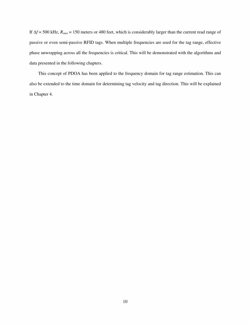
A better approach is to perform a least-square fit analysis of unwrapped phase vs. frequency values.

Linear regression is performed by minimizing the sum of squares of vertical offsets between the phase

values from the linear regression line and the actual measured phase values. The slope of the least-square

best-fit line gives the round-trip travel time. Thus, the range can be estimated as:

Range − estimate�+,+-.= - 4546 *

78π

Here (∆Φ/∆f) is the slope of the best-fit line. Figure 2-4 plots the measured data and the best-fit phase

angle data for different frequencies. The linear fit gives a more accurate estimated slope as compared to

end-point regression. As the number of measurements increases, the slope accuracy and, in turn, the

estimated distance accuracy is expected to improve.

Figure 2-4: Tag range estimation method-1: Unwrapped measured phase angle and best fit angle vs. frequency.

16

Also, using this method the standard deviation of the best fit line can be calculated, which gives the

deviation in radians of the phase values across frequencies. The phase deviation can be translated into

range deviation with respect to a mean range value (which is nothing but the estimated tag range value).

Two standard deviations of the best fit line are considered so that the range answer can be reported as:

Tag range estimate (meters) = mean range estimate ± range deviation with 95% confidence.

The range deviation is calculated as:

Range deviation (meters) = (Standard deviation on best fit line × 2)/ (∆f) × (c/4 × π).

The higher standard deviation indicates that the phase values deviate from the linear trend. This may be

due to environmental effects, antenna characteristics, or other error sources. The standard deviation is an

important indication of the accuracy of the fit and thus of the accuracy of the tag range estimate itself. A

higher standard deviation eventually translates to a larger range interval, and theoretically the actual range

answer should lie somewhere within this estimated range interval with 95% confidence. As noted in [16],

techniques such as goodness of fit can be used to assess the variance of data trends from the straight line.

Calculating the standard deviation of the best fit line is one such technique.

Substituting the values in the equation gives the tag range estimate of 6.220 m, and the tag range

deviation as 0.052 m. Further, the range_reference_estimate is calculated using linear regression and its

value is 5.543 m.

Thus,

Tag range estimate with respect to reference distance = (6.220 – 5.543) m)

= 0.677 ± 0.052 m with 95% confidence

Tag range estimate with respect to antenna = (0.677 + 0.304) ± 0.0522 m with 95 % confidence

= 0.981 ± 0.052m with 95% confidence

Error in tag range estimate = -0.067 m

17

2.2 Processing method 2: Periodic functional fit

This is an alternate processing method for tag range estimation. The basic concept of this method

has been explained in [1]. This method fits the ideal phase angle values corresponding to a “guessed tag

distance” to the measured phase data so as to minimize the square error for each fit. This method does not

require phase unwrapping. Consider the same example explained in Section 2.1

The I-Q phase angle data is obtained from the RFID reader for 50 frequencies and confined to the

range 0 to π. This method tries to fit a periodic function to the produced data set of (Φ,f) values and the

function that best fits the produced data is selected.

A particular value of range Ri is used as a “guessed RFID tag distance” from the RFID reader.

Using this range guess, a data set of ideal I-Q phase angles for each frequency can be calculated using the

relation:

�/+09� = −4π��":;+../c

This data set thus produced ( Φideal, f) for a particular Rguess is then processed to constrain the Φideal within

0 and π. The difference between the calculated and measured phase angles for the entire frequency span is

calculated, and this is also constrained within 0 and π. These differences are squared and summed to find

the sum of the squared errors.

This process is repeated by iterating through several Rguess values, and the functional fit that gives

the least sum of squared errors is selected. The Rguess corresponding to this functional fit is the estimated

tag range. Figure 2-2 in Section 1.2 shows the plot of the measured phase vs. frequency.

Figure 2-5 below shows the error plot for multiple Rguess values, in this case ranging from 0 to 15 m

in incremental steps of 1 mm.

18

Range guess having min sum of squared error

Figure 2-5: Tag Range estimation method-2: Sum of squared errors vs. Range guess

The characteristic periodic nature of the error plot is due to constraining the difference between the

ideal calculated phase angles and the measured phase values between 0 and π. As seen in Figure 2-5, the

intermediate range guesses between the best fit range slope and the near-best fit range slopes have a high

sum of squared errors. Hence, the maximum error values right next to the minimum error values are

observed.

The range guess need only change by a very small value corresponding to a π/2 radians of change

in the calculated phase angle for a particular frequency, say 915.250 MHz, to result in maximum error.

This value is:

Maximum range guess increment step =

<=∗7

�>∗?�@.�@B�CD = 8.2 cm.

The range increments cannot exceed this value. Small increments give better tag range resolution and

accuracy. In the example given the range increment is 1mm.

19

The range guess corresponding to 6.217 m, gives the minimum sum of squared errors. Thus, this is the

estimated tag range.

Figure 2-6 shows the measured and ideal phase angle plot vs. frequency. The ideal phase values are

calculated from the range guess of 6.217 m.

Figure 2-6: Tag range estimation method-2: Measured wrapped phase angle and ideal best fit phase angle vs.

frequency

The range_reference_estimate when the tag is at 0.304 m (1 foot) is calculated using method2, and its

value is 5.493 m.

Thus,

Tag range estimate with respect to reference distance = 0.724 m (6.217 -5.493 m)

Tag range estimate with respect to antenna = 0.724 m + 0.304 m = 1.028 m

Error in range estimate = -0.114 m

Also, similar to method 1 the sum of the squared errors is an indication of the accuracy of the periodic fit

and the tag range estimate.

20

2.3 Further algorithmic details

Section 2.2 and Section 2.3 explained two processing methods for tag range estimation and

presented corresponding examples. Some important points are summarized below which need to be

considered while performing actual algorithmic implementations.

2.3.1 Phase unwrapping

Phase unwrapping is a critical step of the processing method 1. Section 1.4 explains that the

maximum range R that can be determined for a frequency separation of 500 kHz is 150 m. This is to limit

the maximum phase shift between the two frequencies to π radians. The requirement for the maximum

allowable frequency separation can be relaxed with prior knowledge of the maximum tag range according

to the situation. This is calculated by the following equation:

∆fmax_permissible = (c * ∆Φmax ) / (4π*Rmax)

Here, ∆Φmax cannot exceed π radians.

In a real-life implementation, there may be phase dropouts at certain frequencies that result in

incorrect unwrapping. This will be further demonstrated through examples given in Chapter 3, where data

in an open-space setting is obtained. Clearly, phase unwrapping is not needed in processing method 2,

which could be advantageous in certain cases.

2.3.2 Number of phase reads, frequency spacing, and processing time

It is necessary to establish and maintain a balance between the numbers of phase reads for multiple

frequencies and the accuracy and processing time of the algorithm.

The tag range estimation is expected to become more accurate with greater numbers of phase reads, as

multiple reads tend to average out the noise or multipath errors. The EPC Global Class 1 UHF RFID

Protocol for Communications specifies the time required to hop between frequencies while interrogating a

particular tag. Thus, the total time required to estimate the tag range of a particular tag is the summation

21

of times required to singulate a tag, the time required to hop between frequencies (which increases as the

number of frequencies increases), and the time required to calculate the result based on the processing

method used.

In all the tests carried out for this thesis, the full span of the available 50 frequencies is exploited. In

a real application scenario, where the multipath effect is not very severe, fewer frequencies may be a good

choice. In a complicated propagation environment, multifrequency-based techniques with well-designed

frequency-spacing strategies, such as unequal frequency spacing [11], are essential.

Different processing techniques need different processing times for estimating tag range. Method-1

needs less processing time than does method-2. This is because method-2 iterates through the range

guesses, starting from a minimum range guess to a maximum range guess in very small incremental steps

such as 1 mm steps as in the example given. For each of the range guesses, the phase values for all the

interrogated frequencies must be determined, which requires a very time-intensive calculation. Method-1

is the preferred method despite the fact that method-2 does not require phase unwrapping. This is because

a comparison of the two methods shows that method-1 is simpler and more intuitive than method 2, and

method-1 gives metrics to estimate goodness of fit.

2.4 Factors that contribute to errors

This section explains the different sources of errors that may result in errors in tag range estimation.

2.4.1 Hardware errors

The resolution and degree of accuracy of the IQ phase values calculated by the reader from the tag

backscatter signal and the frequency drift of the local oscillator contribute to hardware errors. Either of

these errors can translate to errors in tag range estimation.

Let the phase accuracy of the RFID reader hardware be ±5°. This level of phase accuracy translates

into an error in the range estimation. It is also associated with the total number of phase reads and the

frequency spacing between the reads. This error in tag range estimate is not dependent on the actual range

22

of the tag, i.e., it does not matter if the tag is closer or father away from the antenna, the tag range error in

each case would be the same.

Now, consider each phase value to be normally distributed about its true mean value with a

standard deviation of 5 degrees. In order to calculate the error in tag range due to phase accuracy of the

reader hardware, each phase value for each of the 50 frequencies is generated randomly with a normal

distribution, having mean zero and standard deviation 5 degrees. This would result in a slope value

deviating from the ideal slope value of zero. This process is repeated 1000 times by using the concept of

Monte-Carlo simulation so that 1000 slope values are generated. The mean of the slope values should be

close to zero, and the standard deviation of the slope will translate to an error in tag range estimation.

Note that, as stated earlier, because the tag range error due to the measured phase error is independent of

the actual tag range, the slope of the simulated phase vs. frequency graph is not important.

Figure 2-7 plots the histogram of the slope values generated in this experiment. The histogram has a

normal distribution with a mean slope value of almost zero and a standard deviation of 1.7 × 10−6

radians.

Figure 2-7: Hardware phase error calculation: Histogram of simulated phase angle vs. frequency slopes

23

Based on a concept like the one explained in Section 2.2, in which the standard deviation of the best

fit linear regression line translates to a tag range deviation, this standard deviation of the slope translates

to a range error of 3.31 × 10−6

m, or 0.003 mm.

It is clear that this error contribution is practically negligible. With fewer reads and greater

frequency spacing, this error will increase; however, the value is so small that it can be ignored. The

frequency drift of the local oscillator of the reader is typically about 10 ppm (parts per million). This

would also contribute to a very small error in tag range estimation. Evidently, the algorithm and the

accuracy of the tag range results are not compromised by these hardware errors.

2.4.2 Error due to signal to noise

Another source of IQ phase errors is the Signal to Noise (SNR) error that occurs when the bits of a

tag response are decoded [1]. Averaging across all the EPC bits in the tag response reduces the error,

which is especially significant for a worst-case SNR and thus improves IQ phase accuracy.

2.4.3 Dispersion due to receiver path filters or antenna characteristics

Dispersion is another source of phase IQ angle errors [1]. It is due to antenna characteristics or due

to hardware in the reader receiver path such as the filters. This error is quite small; in fact, it can be

controlled with a good choice of filters and antennas. Usually, this error can also be calibrated out by

using a reference tag distance, as explained in Section 2.1.

2.4.4 Multipath response

In most real-world settings, multipath is present and it is the major factor in causing I-Q phase angle

errors and, in turn, tag range estimation errors. Multipath manifests itself mainly in three broad

mechanisms: reflection, scattering, and diffraction [17].

Reflection occurs when an electromagnetic wave impinges on an object with very large dimensions

compared to the wavelength of propagation. The floor/ground is the main reflective surface, although

24

reflections due to walls and other objects also occur. Scattering occurs when the wave impinges upon

objects in the medium that are smaller in dimensions compared to the wavelength of the impinging RF

wave, such as rough surfaces, small objects, and other irregularities. The direct path ray between the

reader and the tag interferes with the signals that are scattered or reflected, causing significantly large

variations in the amplitude and phase of the received signal. For a reflection that is 10 dB lower compared

to the direct line-of-sight (LOS) path between the tag and the reader, the angle error could be as high as

±tan−1

(0.316/1) = 17.5 degrees [1]. The worst phase error occurs when the non-tag reflection path is 90°

in phase with respect to the tag backscatter path. If the path length changes by even a mere 8 cm (quarter

of a wavelength), the phase shift with respect to the direct ray is 90°.

It is also important to note that it is the signal voltages and not the powers that add. As well as

causing phase errors, the multipath can also cause the RFID tag to receive insufficient power to run its

circuitry and backscatter to the reader at particular spots. Consider two interfering signals 180° out of

phase with respect to the direct LOS signal between the reader and the tag, such that each of the signals

contain 1/10th the power of the direct signal. With the addition of these three signals, the total received

power can change by 12.7 dB, a factor of 20, even though the combined power of the beams is only 20%

of the direct beam [17]. On the other hand, if the signals are in phase with the direct signal, then the

received signal strength at the tag may increase.

In some situations, there is no unimpeded LOS path between the reader antenna and the tag. When

the radio path is obstructed by obstacles of a comparable size to the wavelength, diffraction may occur.

This diffraction gives rise to the bending of waves around the obstacle. In certain situations, it may

prevent the passive tags from being read. This depends on the height of the obstacle and the distance of

the tag from the reader.

Thus, all these mechanisms result in a very complicated propagation environment, especially in

typical office and industrial settings with metal equipment and narrow aisles with metal doors and

concrete floors. These mechanisms cause wild variations in the RSS with small displacements in the

position of the tags or with changes in frequency. Multipath has been characterized and studied in

25

different office settings [19-20], and this can be useful for modeling the distributions and obtaining an

impulse response representative of the environment in order to further our understanding of the multipath

in a given setting.

It is important to note that the multipath is not only a carrier-only signal path; i.e., it not only

includes effects due to reflection and scattering or leakage of the CW-wave RF signal being transmitted to

the tag from the reader, but it also includes tag modulation. The receiver is capable of rejecting the

carrier-only multipath with a good design. This is because the carrier-only multipath components land at

DC after being mixed with the oscillator reference signals. This means fewer possible reflection paths

consisting of paths that pass through the tag reflection backscatter [1].

26

Chapter 3

Collection and Analysis of Tag Range Data in Different Environments

The previous chapter presented the processing methods, algorithmic details, and possible sources of

errors in tag range estimation. To verify and analyze the algorithms and results, tag range estimation is

carried out in three different environments: anechoic chamber, open field, and industrial. All the

experiments are conducted using a single passive RFID tag and a single monostatic reader antenna. The

entire available frequency span of 50 frequencies is utilized, unless stated otherwise.

3.1 Anechoic chamber

RFID tag range estimation tests were carried out in a shielded and anechoic chamber. Designed to

stop reflections of electromagnetic waves, anechoic chambers are insulated from exterior noise sources.

Ideally, the anechoic chamber prevents any effects due to multipath, RF interference, and reflections that

cause errors in range estimation.

The experimental setup consisted of a circularly polarized antenna connected to an RFID reader and

a single passive RFID tag. The RFID tag estimation is carried out starting from the RFID tag at 0.305 m

(1 foot) to 1.752 m (6 feet) from the reader antenna in incremental steps of 0.1524 m (0.5 foot). The tag is

placed along the direction of the bore sight of the antenna. For each distance, the RFID tag is interrogated

over the entire span of 50 frequencies and the tag range is estimated using both method-1 and method-2.

The ‘range_reference_estimate’ is calculated when the tag is at 0.305 m (1 foot). Thus, all the estimated

distances are in reference to the distance of 0.305 m (1foot).

As desired, the phase vs. frequency graphs for each of the experiments is quite smooth and linear;

that is, they show that the anechoic chamber behaves as expected. Figure 3-1 and Figure 3-2 show the

wrapped phase data with periodic functional fit and unwrapped phase data with linear regression obtained

at the tag distance of 0.609 m (2 feet) as an example.

27

Figure 3-1: Anechoic chamber, actual tag distance 0.609 m, method-1range estimation.

Figure 3-2: Anechoic chamber, actual tag distance 0.609 m, method-2 range estimation

28

The tag range estimates calculated by method-1 is plotted in Figure 3-3. Here, as explained in

Section 2.1, the tag range estimate is reported as a mean tag range estimate ± tag range deviation with

95% confidence. This means that effectively the actual tag distance should lie between

tag_range_estimated_minimum to tag_range_estimated_maximum with 95% confidence. Thus, Figure 3-

3 plots the mean tag range estimates, and the spread around each mean value. Negative values of

minimum distances arise because of the requirement to reduce the estimated distance value of the first

point to zero.

Figure 3-3: Anechoic chamber: Calculated tag distance vs. actual tag distance using method-1

29

Figure 3-4 plots the tag range estimated using method 2 shown as below.

Figure 3-4: Anechoic chamber: Calculated tag distance vs. actual tag distance using method-2

3.1.1 Observations

As observed, the estimated tag range vs. actual tag plot follows a general increasing trend. Method

1 performs slightly better than method 2. The estimated tag distances lie close to the true tag distances for

the first 0.914 m (3 feet) of distance, especially as shown in Figure 3-3 for method 1. Beyond 0.914 m (3

feet), the errors are more significant. These errors may be attributable to an imperfect anechoic chamber

setting due to electric noise caused by cables providing a communication link within the chamber. The

type of antenna used and its characteristics may also affect the tag range estimation results.

Table 3-1 summarizes the accuracy of the tag range estimation for the tag range experiment results

in the anechoic chamber. The table reports the standard deviation of the mean tag range estimate vs. the

30

actual tag range graph, the coefficient of determination R2, the average percentage error in the distances

estimated and the values of the smallest and largest error found at given tag distances.

Table 3-1: Accuracy of Tag Range Results in an Anechoic Chamber

As the table shows, the standard deviation of the tag range estimate obtained using method 1 is

0.097 m, and deviation using method 2 is 0.117 m. Both the algorithms give fair result accuracy.

In this experiment, the tag range was estimated only up to 1.752 m (6 feet). In addition, factors such

as interference due to RF cables and human body movements within the chamber were not carefully

controlled. The next section presents the experiments carried out in an open field, where the tag range

estimation was performed for much larger tag distances and in a more controlled fashion.

3.2 Open field

RFID tag range estimation was carried out in an open-field setting. The previous environmental

setting was an anechoic chamber. That experiment aimed to have no potential source of interference from

multipath or noise. In an open field, the only source of interference is the ground plane. Thus, it is a

relatively simple environment in which tag range estimation is expected to have good accuracy. This is

also not a hypothetical setup, as certain real-life uses might be possible in such a setting. Further, the

Setup Standard

Deviation (m)

R2 value Average

percentage

Error

Largest error

(m) at tag

distance (m)

Smallest error

(m) at tag

distance (m)

Anechoic

chamber,

method 1

0.097 m 0.9809 10.5 % 0.286 m at

1.752 m (6

feet)

0.009 at 0.609

m (2 feet)

Anechoic

chamber,

method 2

0.117m 0.9730 11.6 % 0.334 m at 1.6

(5.5 feet)

0.003 at 0.609

m (2 feet)

31

effect of the ground plane as a source of interference is modeled, and its effect on the tag range estimates

observed.

Here, a linearly polarized directional antenna with a 6 dBi gain and a passive RFID tag typically

known to have long read ranges were used. The directional antenna enabled much longer tag read ranges

than would be possible using a dipole antenna. Also, the tag range results for different polarizations and

different reader antenna heights and tag heights are compared. The following four setups are used for the

tag range experiments:

Table 3-2: Setups for tag range experiments in an open field

Setup name

RFID reader

antenna

polarization

RFID tag

polarization

Reader antenna height

above ground m (ft)

Tag height above

ground m (ft)

Setup 1 Horizontal 0.762 (2½) 1.219 (4)

Setup 2 Horizontal 0.762 (2½) 0.610 (2)

Setup 3 Vertical 0.762 (2½) 1.219 (4)

Setup 4 Vertical 0.762 (2½) 0.610 (2)

For each setup, the tag range estimation was carried out for the actual tag distances of 0.305 m (1

foot) to 14.326 m (47 feet) in incremental steps of 0.305 m (1 foot). Also, the tag was placed perfectly

along the direction of the antenna bore sight, such that it would receive maximum incident radiation.

For tag range estimation, the RFID tag at a particular tag distance was interrogated at 50 frequencies to

obtain corresponding phase angle values. The tag range estimation algorithms discussed use only these

returned IQ phase values across frequencies to predict the tag range. Another useful metric is the RSSI of

the backscattered signal received from the tag. The RSSI values can be used as an indication of the tag

range estimate’s accuracy. For each setup, the reader can provide the signal strength or RSSI value of

every tag response at every frequency for each tag distance.

32

Measured signal strength values can be compared with simulated signal strength values for different

setups to both validate the measured values and draw important conclusions about tag range estimates.

Also, this demonstrates an effect of a type of multipath, i.e., ground reflection on the received signal

strength. A signal strength model can be simulated with the knowledge of path loss theory and ground

reflection occurring in an open space setup. The next section addresses the theory of path loss and

propagation in radio communication in open space environments considering the effect of the ground

plane.

3.2.1 Path loss theory and ground-reflection model

Large-scale path loss in an open space is given by the Friis equation:

E� = E ∗ F ∗ F� ∗ � G8H�� ∗ IJ,n=2.

where,

E�: Power available from receiving antenna, E: Power supplied to the transmitting antenna,

F�: Gain in receiving antenna, F: Gain in transmitting antenna

λ: Wavelength, where λ = K6, c = speed of light, and f = frequency

d: Distance

c: Speed of light in vacuum 299.972458·106 [m/s].

The Friis equation describes how the received power at the receiving antenna is dependent on

transmitted power, antenna gain, frequency, and distance. The received power is inversely proportional to

the square of the distance. This free-space propagation model is inaccurate in an open-space setup as this

model does not consider the ground effect. A two-ray ground reflection model is adopted, therefore, as it

is a good method for taking into account the ground effect.

33

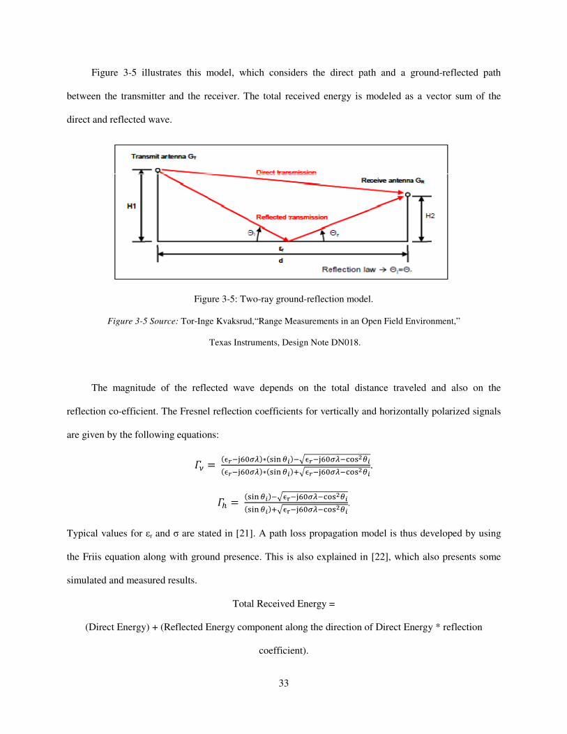
Figure 3-5 illustrates this model, which considers the direct path and a ground-reflected path

between the transmitter and the receiver. The total received energy is modeled as a vector sum of the

direct and reflected wave.

Figure 3-5: Two-ray ground-reflection model.

Figure 3-5 Source: Tor-Inge Kvaksrud,“Range Measurements in an Open Field Environment,”

Texas Instruments, Design Note DN018.

The magnitude of the reflected wave depends on the total distance traveled and also on the

reflection co-efficient. The Fresnel reflection coefficients for vertically and horizontally polarized signals

are given by the following equations:

LM = �NOPQRCSG�∗�.�� TU�PVNOPQRCSGP7W.=TU�NOPQRCSG�∗�.�� TU�XVNOPQRCSGP7W.=TU

.

LY = �.�� TU�PVNZPQRCSGP7W.=TU�.�� TU�XVNZPQRCSGP7W.=TU

.

Typical values for εr and σ are stated in [21]. A path loss propagation model is thus developed by using

the Friis equation along with ground presence. This is also explained in [22], which also presents some

simulated and measured results.

Total Received Energy =

(Direct Energy) + (Reflected Energy component along the direction of Direct Energy * reflection

coefficient).

34

The Direct Energy and Reflected energy are calculated using the Friis transmission formula, where

the distance (d) becomes I/�-+7,P[0\+ and I-+]9+7,+/P[0\+ as follows:

I/�-+7,P[0\+ = Vabs�ℎ� − ℎ��� + I�

I-+]9+7,+/P[0\+ = V�ℎ� + ℎ��� + I�

The phase difference between the direct and reflected wave can be calculated from the path difference ∆d

as follows:

phase difference = 2πΔI fg , where ΔI (Path difference) = I/�-+7,P[0\+ – I-+]9+7,+/P[0\+.

Given this knowledge of the phase difference, we can find the component of the reflected wave along the

direct wave to obtain the total received energy at a distance d from the transmitter.

For this model, the electric field energy received at the RFID reader by the travel of the RF wave to

the RFID tag and back is simulated for each setup. As the RF wave travels from the reader antenna to the

tag and back from the tag to the reader antenna, this model is applied in two steps. First, the two-ray

model is used to calculate the energy received, say E�h_jk at the RFID tag at a distance d from the

antenna. Following this step, the RF wave with energy E�h_jk again has to travel a distance d back to the

reader antenna. For this, Eh_jk = 0.1 ∗ E-B_,0: , and once again the two-ray model is applied, which

finally gives E�h_�mjnm� . The factor of 0.1 is considered, as passive tags backscatter only about 10% of

their incident energy.

In all the simulations the transmitted power from the RFID reader antenna is 1 watt, the gain of the

RFID reader antenna = 6 dBi and the gain of the tag antenna is unity. The values of εr = 15 and σ = 0 are

chosen based on soil conditions.

3.2.2 Data collection and results

This section presents the tag range estimation results along with the measured and simulated signal

strength plots for each of the four setups. The data and results for setup-1 (horizontally polarized antenna

and tag with a tag height of 1.219 m (4 feet) are explained in detail. Certain improvements to the

35

processing method are also elaborated. Following this, the data and results for the other three setups are

also presented. In all the setups the range_reference_estimate is calculated when the tag is at 0.3048 m (1

foot). Thus, all the estimated distances are in reference to the distance of 0.305 m (1foot).

Now consider setup-1. Figure 3-6 plots the mean tag range estimates, and the spread around each

mean value obtained by method-1.

Figure 3-6: Open-field setup-1, calculated tag distance vs. actual tag distance using method-1.

.

36

Figure 3-7 plots the estimated tag distance obtained by method-2 and the actual tag distance.

Figure 3-7: Open-field setup-1: Calculated tag distance vs. actual tag distance using method-2.

Figures 3-6 and 3-7 show that the tag range values estimated by method-1 as well as method- 2 are

very close to the true tag distances. Also, Figure 3-6 shows that the tag range deviation calculated from

the standard deviation on the best fit linear regression line is generally very small, which suggests that the

std. deviation of each of the phase vs. frequency plots for each tag distance is also low. Let us consider

the tag range estimates for the actual tag distances of 4.77 m (15 feet) m and 5.18 m (16 feet). Here, the

mean tag range estimate from method 1 and also the tag range estimate from method 2 have larger errors

compared to the estimates from the other locations. The tag range deviation is also higher. Figure 3.6

makes this evident.

To analyze the results of the tag range experiment a

frequency plot obtained at the tag distance of 5.18 m is plotted in Figure 3

comparison, the phase vs. frequency graph at the tag distance of 2.13 m is also plotted in Figure 3

Figure 3-8: Open-field setup

Figure 3-9: Open-field setup

37

To analyze the results of the tag range experiment at these locations, the wrapped phase vs.

frequency plot obtained at the tag distance of 5.18 m is plotted in Figure 3-8. For the purpose of

comparison, the phase vs. frequency graph at the tag distance of 2.13 m is also plotted in Figure 3

field setup-1: measured phase angle vs. frequency for tag distance 5.18 m.

field setup-1: Measured phase angle vs. frequency for tag distance 2.13 m.

t these locations, the wrapped phase vs.

8. For the purpose of

comparison, the phase vs. frequency graph at the tag distance of 2.13 m is also plotted in Figure 3-9.

1: measured phase angle vs. frequency for tag distance 5.18 m.

Measured phase angle vs. frequency for tag distance 2.13 m.

38

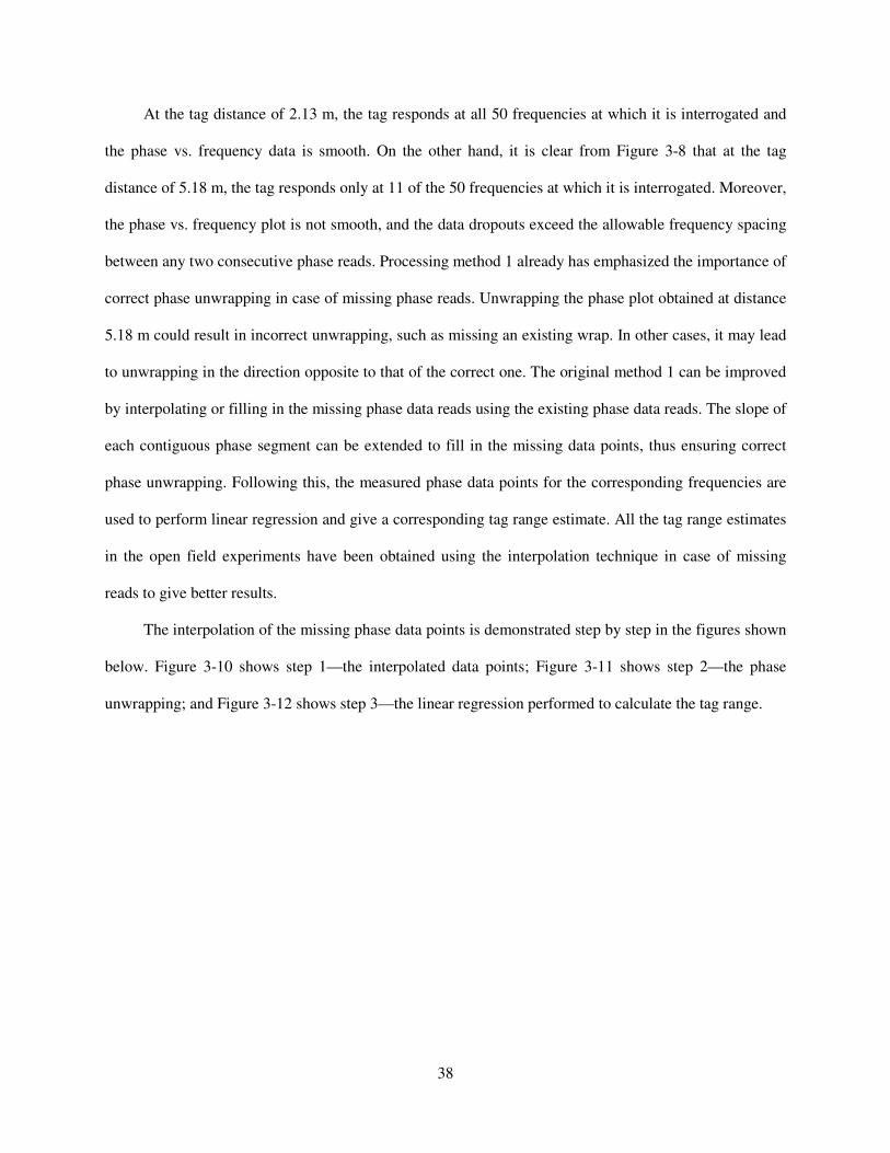
At the tag distance of 2.13 m, the tag responds at all 50 frequencies at which it is interrogated and

the phase vs. frequency data is smooth. On the other hand, it is clear from Figure 3-8 that at the tag

distance of 5.18 m, the tag responds only at 11 of the 50 frequencies at which it is interrogated. Moreover,

the phase vs. frequency plot is not smooth, and the data dropouts exceed the allowable frequency spacing

between any two consecutive phase reads. Processing method 1 already has emphasized the importance of

correct phase unwrapping in case of missing phase reads. Unwrapping the phase plot obtained at distance

5.18 m could result in incorrect unwrapping, such as missing an existing wrap. In other cases, it may lead

to unwrapping in the direction opposite to that of the correct one. The original method 1 can be improved

by interpolating or filling in the missing phase data reads using the existing phase data reads. The slope of

each contiguous phase segment can be extended to fill in the missing data points, thus ensuring correct

phase unwrapping. Following this, the measured phase data points for the corresponding frequencies are

used to perform linear regression and give a corresponding tag range estimate. All the tag range estimates

in the open field experiments have been obtained using the interpolation technique in case of missing

reads to give better results.

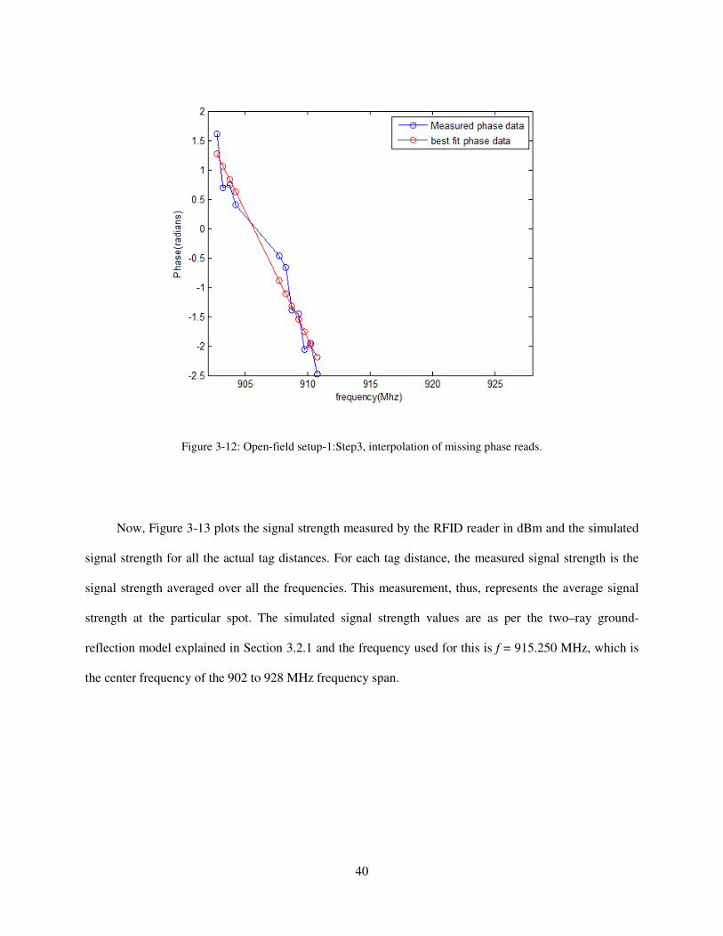
The interpolation of the missing phase data points is demonstrated step by step in the figures shown

below. Figure 3-10 shows step 1—the interpolated data points; Figure 3-11 shows step 2—the phase

unwrapping; and Figure 3-12 shows step 3—the linear regression performed to calculate the tag range.

Figure 3-10: Open

Figure 3-11: Open field setup

39

field setup-1: Step1, interpolation of missing phase reads.

11: Open field setup-1: Step2, interpolation of missing phase reads.

1: Step1, interpolation of missing phase reads.

1: Step2, interpolation of missing phase reads.

40

Figure 3-12: Open-field setup-1:Step3, interpolation of missing phase reads.

Now, Figure 3-13 plots the signal strength measured by the RFID reader in dBm and the simulated

signal strength for all the actual tag distances. For each tag distance, the measured signal strength is the

signal strength averaged over all the frequencies. This measurement, thus, represents the average signal

strength at the particular spot. The simulated signal strength values are as per the two–ray ground-

reflection model explained in Section 3.2.1 and the frequency used for this is f = 915.250 MHz, which is

the center frequency of the 902 to 928 MHz frequency span.

41

Figure 3-13: Open-field setup-1: Measured and simulated RSSI vs. actual tag distance.

The measured RSSI and simulated RSSI graphs follow the same trend: the measured and simulated

RSSI values dip in the same tag distance spots, which demonstrate the effect of the ground presence on

the RSSI. Also, it is observed that the measured and simulated RSSI both dip significantly at tag distances

of 4.77 m and 5.18 m. These are the same spots where the estimated tag range deviates from the actual

range, as explained above. At the distance of 5.18 m, the average RSSI value is −75 dBm. The read

sensitivity of passive tags is generally between 70 to 75 dBm (this is the value of the backscattered tag

response signal strength). Below this threshold, the tag may not receive sufficient power to decode the

reader data and so backscatter its response, or the tag backscattered response maybe too weak to be

demodulated by the reader. As has already been seen, at the distance of 5.18 m the tag responds only at

certain frequencies. Moreover, the phase is more sensitive to noise when the signal strength is low. The

accuracy of the tag range estimate thus depends on factors such as RSSI, the total number of phase reads,

and the standard deviation about the best fit line of the phase vs. frequency plot, as estimated by

processing method 1.

42

With this background, the results for the remaining three setups are presented. Here, the tag range

results estimated only by processing method-1 are plotted. As seen in the earlier section, method-2 yields

results that are similar to those of method-1. However, method 1 is the preferable processing method as

explained in Section 2.3.2.

Figure 3-14 plots the mean tag range estimates, and the spread around each mean value obtained by

method-1 and Figure 3-15 shows plots the measured and simulated RSSI values for tag distances for

setup-2.

Figure 3-14: Open-field setup-2: Calculated tag distance vs. actual tag distance using method-1.

43

Figure 3-15: Open field setup-2: Measured and simulated RSSI vs. actual tag distance.

44

Figure 3-16 plots the mean tag range estimates, and the spread around each mean value obtained by

method-1 and Figure 3-17 shows plots the measured and simulated RSSI values for tag distances for

setup-3.

Figure 3-16: Open field setup-3: Calculated tag distance vs. actual tag distance using method-1

45

Figure 3-17: Open field setup-3: Measured and simulated RSSI vs. actual tag distance.

Figure 3-18 plots the mean tag range estimates, and the spread around each mean value obtained by

method-1 and Figure 3-19 shows plots the measured and simulated RSSI values for tag distances for

setup-4. In these, the tag estimates for distances beyond 11.583 m (38 feet) are not plotted. This is

because the number of phase reads obtained for each of these distances is fewer than 5 reads, and in some

cases the tag does not respond at any frequency giving zero reads.

46

Figure 3-18: Open field setup-4: Calculated tag distance vs. actual tag distance using method-1

47

Figure 3-19: Open field setup-4: Measured and simulated RSSI vs. actual tag distance.

3.2.3 Observations

The results obtained from experiments conducted in an open space clearly show that the tag range

estimation performs well in such a setting. The two-ray ground-reflection model is useful for analyzing

the behavior of a tag that located in a bad spot. There are some shifts, though, between the simulated

RSSI graphs and the corresponding measured RSSI graphs. A number of factors such as the properties of

the tag, the near field conditions for closer tag distances, and the behavior of the tag electronics for higher

field strengths that could be responsible for this offset. Despite these offsets, the model does give a fair

demonstration of the effects of multipath considering the simplest of conditions— the ground bounce ray.

Table 3-2 summarizes the accuracy of tag range estimation for all four setups in open space. This is

similar to Table 3-1, which summarizes the accuracy of tag range estimation for the anechoic chamber.

48

Table 3-3: Accuracy of Tag Range Results in Open Space

Setup Standard

Deviation

(m)

R2 value Average

percentage Error

Largest error (m) at

tag distance (m)

Smallest error

(m)at tag distance

(m)

Setup1 0.187 m 0.998 4.3 % 0.774 m at 13.106 m

(43 feet)

0.016 at 3.050 m

(10 feet)

Setup2 0.336 m 0.994 5.3 % 2.221 m at 13.106 m

(43 feet)

0.027 at0.610 m (2

feet)

Setup3 0.493 m 0.989 8.6 % 3.2064 m at 13.106

m

(43 feet)

0.003 m at 1.2192

m

(4 feet)

Setup4 0.679 m 0.966 8.1 % 3.397 at 11.887 m

(39 feet)

0.008 at 0.914 m (3

feet)

As can be seen from Table 3-2, the standard deviation for setup 1 is 0.187 m, which is just over half

a foot. This is very good result accuracy. Setup-4 has the highest deviation of 0.679 m, which is just over

2 feet. Also, the average percent error for all the setups is well below 10 % - setup 1 has an average

percent error as low as 4.3.

These results validate the feasibility of the tag range estimation algorithms in open spaces and in settings

with low multipath.

3.3 Industrial setting

This section illustrates the tag range estimation experiments carried out in a typical industrial

setting. The industrial setting consists of walls and concrete floors, which act as reflectors, and also metal

doors and cabinets, and surrounding objects and equipment, all of which result in a high-multipath

environment.

Tag range experiments are conducted in this setting. Tag range estimation is carried out at actual

tag distances, starting at 0.305 m (1 foot) from the reader antenna to 5.182 m (17 feet), in incremental

49

steps of 1 foot. Similar to procedures set out in the previous settings, the range_reference_estimate is

calculated when the tag is at 0.305 m (1 foot). All the estimated distances are in reference to the distance

of 0.305 m (1foot).

Figure 3-20 plots the mean tag range estimates, and the spread around each mean value obtained by

method-1. As in the previous section, which focuses on an open-space setting, interpolation of missed

phase reads is incorporated for better results.

Figure 3-20: Industrial setup: Calculated tag distance vs. actual tag distance using method-1.

Figure 3-21 plots the measured RSSI averaged across all frequency values vs. the actual tag

distances.

Figure 3-21: Industrial setting: Measured and simulated RSSI vs. actual tag distance.

3.3.1 Observations

The tag range estimates are close to the true tag range for the first

distance, though, the error in tag range estimate increases. Multipath interference is the factor that

contributes most to errors. Moreover, the RSSI plot demonstrates that the RSSI is always above the read

tag sensitivity level, yet, despite this, the total number of phase reads drops and the tag range estimates

become less accurate for tag distances beyond

The propagation environment is extremely complex in such high

measures like avoiding metal objects in the surrounding could help improve performance.

Table 3-4 summarizes the accuracy of tag range estimates for the industrial setting. The table

reports the standard deviation of the mean tag range estimate vs. actual tag range line, the co

determination R2 value, and the smallest and largest errors reported at the actual tag distances.

50

21: Industrial setting: Measured and simulated RSSI vs. actual tag distance.

The tag range estimates are close to the true tag range for the first 1.829 m (6 feet).

distance, though, the error in tag range estimate increases. Multipath interference is the factor that

contributes most to errors. Moreover, the RSSI plot demonstrates that the RSSI is always above the read

this, the total number of phase reads drops and the tag range estimates

become less accurate for tag distances beyond 1.829 m (6 feet).

The propagation environment is extremely complex in such high-multipath environments. Certain

tal objects in the surrounding could help improve performance.

summarizes the accuracy of tag range estimates for the industrial setting. The table

reports the standard deviation of the mean tag range estimate vs. actual tag range line, the co

value, and the smallest and largest errors reported at the actual tag distances.

21: Industrial setting: Measured and simulated RSSI vs. actual tag distance.

m (6 feet). Beyond this

distance, though, the error in tag range estimate increases. Multipath interference is the factor that

contributes most to errors. Moreover, the RSSI plot demonstrates that the RSSI is always above the read

this, the total number of phase reads drops and the tag range estimates

multipath environments. Certain

tal objects in the surrounding could help improve performance.

summarizes the accuracy of tag range estimates for the industrial setting. The table

reports the standard deviation of the mean tag range estimate vs. actual tag range line, the co-efficient of

value, and the smallest and largest errors reported at the actual tag distances.

51

Table 3-4: Accuracy of Tag Range Results in an Industrial Setting

It is clear from the table that the results have a high standard deviation or overall error; i.e., the error

is 1.242 m, even for the first 5.182 m (17 feet) of distance. The percentage error is 26.7 %, which is

evidently high as it includes the error contribution due to the largest tag range error which occurs at the

tag distance of 15 feet. The smallest error in tag range estimation is at 5.182 m (17 feet) and the largest

error is at 4.572 m (15 feet), which demonstrates the effect of multipath as the tag moves by less than a

meter of distance.

Setup Standard

Deviation (m)

R2

value

Average

percentage error

Largest Error (m)

at Tag distance (m)

Smallest

Error (m) at

Tag distance

(m)

Industrial

Setting

method1

1.242 m 0.727 26.7 % 4.385 m at 4.572 m

(15 feet)

0.025 m at

5.182 m

(17 feet)

52

Chapter 4

Tag Motion/Velocity and Direction Estimation

Chapters 1 and 2 provided insight into the theory on which tag range estimation is based, in which a

fixed RFID tag is singulated and interrogated at multiple frequencies to obtain corresponding I-Q phase

values. This data is then further processed to give a tag range estimate with respect to the RFID reader.

The Phase Difference of Arrival technique can also be used to determine tag motion or tag direction and

radial tag velocity with respect to the reader antenna.

This chapter will provide a mathematical introduction to tag motion estimation, followed by

explanation of data processing techniques. Data for tag motion estimation collected in an industrial setting

for different situations are presented along with analysis and suggestions for algorithmic improvements. A

real-life use case which estimates motion of people walking through a portal is also presented, which uses

an alternative data processing technique of Kalman filtering.

4.1 Mathematical introduction to tag range estimation

Consider a fixed tag or a tag at the same radial distance with respect to the reader antenna being

singulated and interrogated at a single frequency multiple times at successive time instants. If the obtained

I-Q angles are observed as a function of time, their value remains the same. If the tag is moving towards

the reader, the phase I-Q angle rotates in a clockwise direction as a function of time, whereas if the tag is

moving away from the reader, the phase I-Q angle rotates in the opposite direction, i.e., counter-clockwise

direction. The directions are as per the reader equipment being used. Thus, it can be can determined if a

tag is moving towards or away from the reader antenna by interrogating a tag at the same frequency

multiple number of times.

To explain this mathematically, consider the example illustrated in Section 1.4, with the

modification that the RFID tag is now in motion with respect to the RFID reader antenna instead of being

at a fixed location. At time instances t1 and t2, the RFID reader singulates and interrogates the tag twice at

a fixed frequency fi. The tag backscatters the signal and this is received at the RFID tag reader as:

53

����� = ρ� exp�−jo� �o��� , i = 1, 2,

This result has the same meaning as explained in Section 1.4, i.e., u(t) is the waveform transmitted from

the reader, !o and o are the amplitude and phase of the return signal.

As has been established, the returned I-Q phase of the signal is frequency and range-dependent. Here

frequency is constant and range or distance is a variable. The phase can be expressed as:

� = 4π�"i/c.

As the tag is in motion, the range is variable and can be expressed as Ri = vti, assuming the velocity is

constant. The equation can be re-written as:

Φi = (4πftiv)/c

With the knowledge of the phase difference of the return signals at time instants t1 and t2, the velocity (v)

of the moving tag can be estimated as:

v = (cΔΦ)/ (4πfΔt) and, ΔΦ= Φ1 – Φ2 and Δt = t2-t1.

The sign of the velocity value indicates the direction in which the tag is moving with respect to the reader.

According to the behavior of the IQ phase obtained from the reader and as per the convention followed in

the thesis, a positive velocity sign implies that the RFID tag is moving towards the reader, whereas a

negative velocity sign implies that the RFID tag is moving away from the reader.

The mathematical formulation above explains velocity and direction estimation calculated using

two phase values obtained for two different time instances on a single tag in motion. Processing multiple

phase values for multiple time instances and keeping the frequency constant would give a more accurate

tag velocity and tag direction estimate.

4.2 Processing method: End-point regression and linear regression

The processing technique for tag velocity and direction estimation is inherently similar to that

explained in Section 2.1 for tag range estimation. An RFID tag in motion is singulated and interrogated at

a particular frequency fn in the range of 902 to 928 MHz at multiple time instances to obtain

54

corresponding phase angles or IQ rotator angles from the reader. These angles are confined to the range 0

to π to resolve the phase ambiguity..

Figure 4-1 demonstrates the modulo π data phase data collected on a single RFID tag in motion that

is moving away from the RFID reader antenna placed on a track moving at the speed of 0.21 m/s. In this

example, the total data capture is for about 0.9 seconds, and it starts with the tag at an initial distance of

0.305 m (1 foot) from the reader antenna and the tag is moving away from it. Thus, in 0.9 seconds, the tag

covers a distance of only about 0.2 m. The tag is interrogated at the frequency 902.250 MHz at 25

successive time instants, reasonably uniformly spaced at about 30–35 msec. apart.

Figure 4-1: Wrapped measured phase angle vs. time for tag moving away from antenna.

The IQ phase vs. time plot is unwrapped appropriately by subtracting π from all phase values after

encountering a wrap in this particular example. Similar to the tag range algorithms, unwrapping is a

critical step. The maximum speed that can be determined for effective phase unwrapping is dictated by

the time separation between consecutive phase values.

55

The slope of the unwrapped phase values across time instants is used to calculate the velocity of the

tag according to the equation above. The slope can be determined using end-point regression, a simple

technique that considers only the end-points of the phase graph and is, therefore, susceptible to end-point

errors. The second approach, as explained in the tag range processing algorithm, is to perform a least-

square fit analysis on the phase graph in order to obtain a more accurate slope.

Figure 4-2 shows the unwrapped phase plot, along with linear regression performed to give a best fit line.

Figure 4-2: Unwrapped measured phase angle and best fit phase angle vs. time for tag moving away from antenna.

The velocity can be calculated from the slope (∆Φ/∆t) of the best fit line. This method also gives a

standard deviation on the best fit line which translates into a velocity deviation. The velocity deviation

can be calculated as:

Velocity_deviation (meters) = (Std_deviation_on_best_fit_line * 2)/(Δt) * (c/4πf).

The velocity can be reported as

mean_estimated_velocity ± velocity_deviation with 95% confidence.

56

Thus, for this particular example,

Velocity of the tag = -0.201 m/s ± 0.007 m/s with 95 % confidence

Error in tag velocity estimate = -0.009 m/s

The tag motion estimation experiment is repeated with the same setup, but with the RFID tag moving

towards the reader antenna and starting at an initial position of 0.914 m (3 feet) from the reader antenna.

Figure 4-3 shows the unwrapped phase vs. time plot that results in a positive slope as against the negative

slope in the previous figure.

Figure 4-3: Unwrapped measured phase angle and best fit phase angle vs. time for tag moving towards the antenna

Thus in this example,

Velocity of the tag = 0.251± 0.006 m/s with 95 % confidence

Error in estimate = 0.041 m/s

57

4.3 Further algorithmic details

This section summarizes some important points that need to be considered during algorithmic

implementations.

4.3.1 Phase unwrapping

Accurate phase unwrapping is critical in order to establish the correct tag velocity and direction

estimation. The time separation between consecutive phase reads should be such that the phase difference

between the reads for a tag moving at a particular velocity should not exceed π radians, otherwise there is

a possibility of missing a wrap or incorrect phase unwrapping.

The condition for a maximum allowable phase difference of ∆Φmax = π radians together with the

time spacing between consecutive phase reads dictate the maximum radial speed at which the tag can

move for the tag velocity or tag direction estimation algorithm to produce accurate results. Thus,

Maximum velocity limit of tag = (π* 3x108) / (4π* 915.250 x 106 * Δt)

The time difference ∆t between successive phase acquisitions at a particular frequency depends on

the capabilities of the RFID reader and on the protocol requirements. Figure 4-4 plots the maximum

velocity limit of tag vs. time difference for consecutive phase reads according to the equation above. As

evident from the figure, as the phase reads become closer together, so the maximum velocity limit

increases.

58

Figure 4-4: Maximum velocity limit vs. time difference between consecutive reads.

Now, similar to the maximum tag speed limit, there is a minimum radial speed limit at which the

tag should be moving for the algorithm to detect a phase change across time instances and estimate

velocity and direction. If the RFID tag is moving slowly and the data capture is done at a very fast rate, it

is possible that the phase change over time will not be detected, resulting in an incorrect direction

estimate and an error in velocity.

The phase needs to change by some minimum value between consecutive phase reads. This limit

depends on the phase accuracy of the reader. For a phase accuracy of 5 degrees or 0.087 radians, ∆Φ

between consecutive time instances should be greater than 0.087 radians. Hence, we choose here ∆Φ =

0.1 radians. Thus,

Minimum velocity limit of tag = (0.1 * 3x108) / (4π * 915.250 x106 * Δt)

Figure 4-5 plots the minimum velocity limit of tag vs. time difference for consecutive phase reads

according to the equation above. As evident from the figure, as the phase reads become farther apart, so

the minimum velocity limit decreases.

Figure 4-5: Minimum velocity limit vs. time difference betw

This equation and the resulting minimum velocity bound is conservative, which necessitates that the

phase change between consecutive phase reads be at least 0.1 radians. This bound can be relaxed

considering that even an overall phase change of 0.1 radians across several time instances maybe suitable

for reliable velocity/direction estimation.

Thus, the time separation ∆t between consecutive reads should be selected according to specific

uses classified according to tag speeds. For

maximum tag speed limit is around 81 m/s while the minimum speed limit is 2.6 m/s. This

applications like determining the speed of cars passing through a toll booth, but not for app

the motion of tagged objects has to be estimated in an inventory in which the speed of the tag in mo

might be lower than the speed of 2.6 m/s.

It is important to note also that there might be phase dropouts on a particular tag

velocity is being determined. Therefore, phase dropouts must be taken care of, as this might mean that the

time difference between consecutive phase reads exceeds the allowable maximum time difference limit.

59

5: Minimum velocity limit vs. time difference between consecutive reads.

This equation and the resulting minimum velocity bound is conservative, which necessitates that the

phase change between consecutive phase reads be at least 0.1 radians. This bound can be relaxed

ase change of 0.1 radians across several time instances maybe suitable

for reliable velocity/direction estimation.

∆t between consecutive reads should be selected according to specific

uses classified according to tag speeds. For example, if Δt is 1 ms between successive phase reads, the

maximum tag speed limit is around 81 m/s while the minimum speed limit is 2.6 m/s. This

speed of cars passing through a toll booth, but not for app

the motion of tagged objects has to be estimated in an inventory in which the speed of the tag in mo

be lower than the speed of 2.6 m/s.

that there might be phase dropouts on a particular tag

Therefore, phase dropouts must be taken care of, as this might mean that the

time difference between consecutive phase reads exceeds the allowable maximum time difference limit.

een consecutive reads.

This equation and the resulting minimum velocity bound is conservative, which necessitates that the

phase change between consecutive phase reads be at least 0.1 radians. This bound can be relaxed

ase change of 0.1 radians across several time instances maybe suitable

t between consecutive reads should be selected according to specific

is 1 ms between successive phase reads, the

maximum tag speed limit is around 81 m/s while the minimum speed limit is 2.6 m/s. This is suitable for

speed of cars passing through a toll booth, but not for applications where

the motion of tagged objects has to be estimated in an inventory in which the speed of the tag in motion

that there might be phase dropouts on a particular tag in motion whose

Therefore, phase dropouts must be taken care of, as this might mean that the

time difference between consecutive phase reads exceeds the allowable maximum time difference limit.

60

4.3.2 Number of phase reads, time spacing, and processing time

There is a fine trade-off between the desired accuracy of the algorithm and processing time. Similar

to tag range algorithms, multiple phase reads are likely to give a more accurate estimate of the tag’s

velocity/direction. This is especially true in complicated propagation environments, as in such

environments, it provide an averaging of noise and multipath errors. As explained in the earlier section, if

the batch of tags whose motion has to be estimated comprises fast-moving tags, the phase reads need to

be closely spaced; however, for a batch of very slow-moving tags, the phase reads are spaced at

comparatively much larger time intervals. The total time spent to acquire data on a slow-moving tag,

therefore, will be greater than for a fast-moving tag. In a real-life scenario, dwelling on a slow particular

tag for too long may cause other tags, especially fast-moving tags, to disappear out of the read range of

the antenna.

4.4 Factors that contribute to errors

Section 2.4 explains the different sources of error which cause errors in tag range estimation. The

same errors also affect the tag motion estimation results.

The resolution of the I-Q phase values and also of the timestamp value reported by the reader result

in errors in tag motion estimation, these can be calculated in a similar fashion to that in Section 2.4.1.

Multipath remains the dominant cause of errors in tag motion estimation.

4.5 Data collection in industrial setting and analysis

The tag range experiments have already been carried out in different environmental settings and

have demonstrated the effects of multipath in an industrial environment. The same performance issues for

tag motion estimation arise. This section further presents and analyzes data collected in certain situations.

61

4.5.1 Situation-1

The previous examples demonstrated how velocity and direction are estimated on a single RFID

tag. The data is collected when the tag is within 0.305 m (1 foot) to 0.914 m (3 feet) of the antenna. A

similar experiment is repeated with a single tag on the track moving away from the reader at the speed of

0.21 m/s. In this case, the data is collected starting at 3 feet to about 12 feet of the reader antenna. All the

data is collected at a single frequency, fn = 904.250 MHz. Note that this data is collected in the same

industrial setting as the tag range experiments described in Section 3.3. Figure 4-6 demonstrates the data

collected, along with a best fit line obtained by running linear regression whose slope translates into

velocity and the standard deviation translates into velocity deviation.

Figure 4-6: Situation-1: Unwrapped measured phase angle and best fit phase angle vs. time for tag moving away

from the antenna for a large time interval.

Large numbers of phase reads (the tag is interrogated 250 times) are collected for a time span of

about 11 seconds. This gives the following velocity estimate:

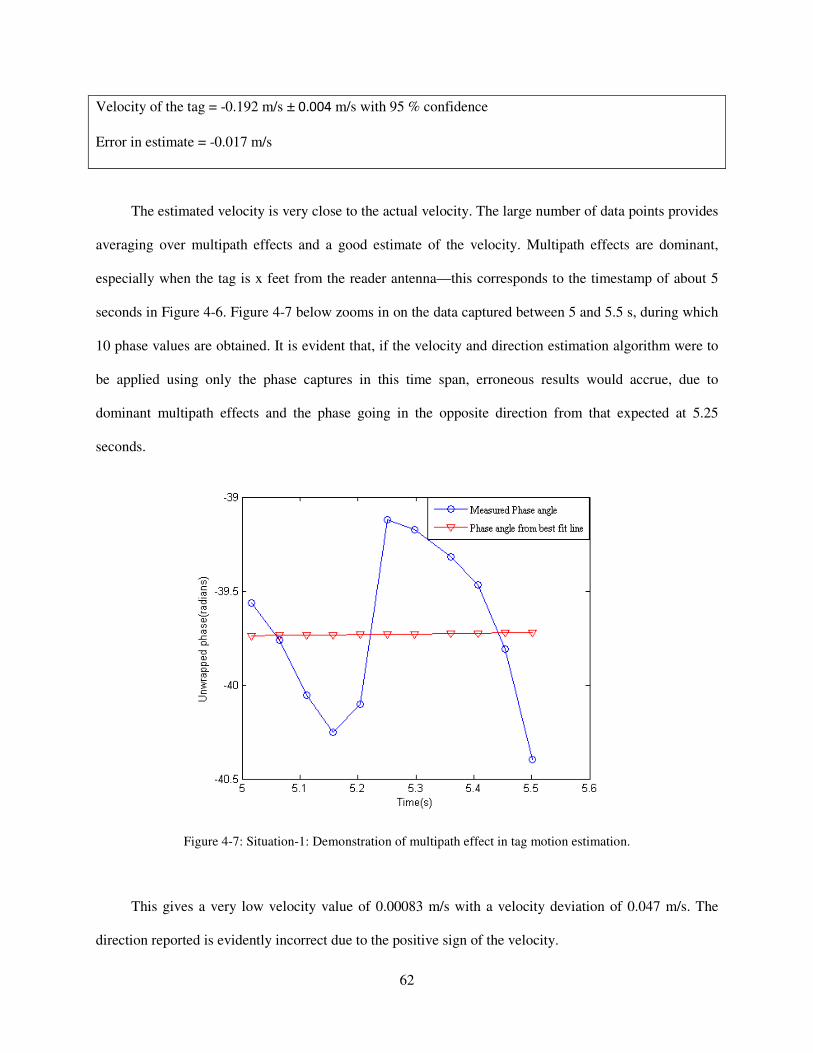
62

Velocity of the tag = -0.192 m/s ± 0.004 m/s with 95 % confidence

Error in estimate = -0.017 m/s

The estimated velocity is very close to the actual velocity. The large number of data points provides

averaging over multipath effects and a good estimate of the velocity. Multipath effects are dominant,

especially when the tag is x feet from the reader antenna—this corresponds to the timestamp of about 5

seconds in Figure 4-6. Figure 4-7 below zooms in on the data captured between 5 and 5.5 s, during which

10 phase values are obtained. It is evident that, if the velocity and direction estimation algorithm were to

be applied using only the phase captures in this time span, erroneous results would accrue, due to

dominant multipath effects and the phase going in the opposite direction from that expected at 5.25

seconds.

Figure 4-7: Situation-1: Demonstration of multipath effect in tag motion estimation.

This gives a very low velocity value of 0.00083 m/s with a velocity deviation of 0.047 m/s. The

direction reported is evidently incorrect due to the positive sign of the velocity.

63

Also, it can be observed from Figure 4-6 that no phase reads are recorded between 9.6 and 10.2 s,

either due to the tag’s failure to power up, or due to insufficient signal strength received at the reader

caused by multipath or frequency nulls for the particular frequency at the particular location. If the tag

motion algorithm were to be applied only during this interval at the same frequency, no phase reads

would be obtained and no report would accrue.

4.5.2 Situation-2

All the previous examples involved finding direction/velocity for a single RFID tag. Consider a

case that is closer to a real-life application scenario; that is, a situation in which this algorithm is run for

multiple RFID tags. In this experiment, 10 tags are moving on a track at a fixed speed of 0.21 m/s, such

that 5 tags are moving towards the antenna and 5 tags are moving away from it. Each tag is singulated and

interrogated 10 times to obtain 10 phase reads. The order in which these tags are singulated to obtain

phase reads is depicted in Figure 4-8 below, where the number on the x-scale represents the order of

singulation. Also, the frequency of the carrier wave is fixed at f = 904.250 MHz.

Figure 4-8 plots the signed velocity results for each of the 10 tags, where the velocity is reported

within a velocity range, i.e., from minimum estimated velocity to maximum estimated velocity for each

tag. Also, the horizontal bar drawn in the figure represents the tags’ actual velocity of 0.21 m/s.

Figure 4-8: Situation-2: Velocity estimation for 10 tags: Velocity (m/s) vs. tag numb

As observed for tag 5, which is actually moving towards the antenna, the velocity is a very small

number. This tag responds only 4 of the 10 times it is interrogated. Further, for tag 6, which is moving

away from the antenna, no reads are obtained; he

tags 5 and 6 are affected by multipath effects when they are being interrogated.

The direction of the remaining 8 tags is reported correctly, and the velocity error is as observed

from the figure. It is clear that in this case, direction is reported correctly 80% of the time, and a similar

level of accuracy is expected in other industrial settings.

detuning effects may also cause additional errors in the resul

Several improvements could be made to the algorithm to obtain better results.

improvement could be frequency hopping, when no response is obtained from a particular tag

at a particular frequency. To demonstrate this basic concept, c

motion interrogated at a fixed frequency

This interrogation is then repeated with the same setup, but at the fixed frequency

-0.4

-0.3

-0.2

-0.1

0

0.1

0.2

0.3

0.4

1

64

Velocity estimation for 10 tags: Velocity (m/s) vs. tag numb

As observed for tag 5, which is actually moving towards the antenna, the velocity is a very small

This tag responds only 4 of the 10 times it is interrogated. Further, for tag 6, which is moving

away from the antenna, no reads are obtained; hence, the velocity/direction cannot be reported.

tags 5 and 6 are affected by multipath effects when they are being interrogated.

The direction of the remaining 8 tags is reported correctly, and the velocity error is as observed

is clear that in this case, direction is reported correctly 80% of the time, and a similar

level of accuracy is expected in other industrial settings. Due to the presence of multiple tags, tag

detuning effects may also cause additional errors in the results.

Several improvements could be made to the algorithm to obtain better results.

could be frequency hopping, when no response is obtained from a particular tag

at a particular frequency. To demonstrate this basic concept, consider Figure 4-9, which shows a tag in

motion interrogated at a fixed frequency f1= 910.250 MHz while moving from position a to position b.

This interrogation is then repeated with the same setup, but at the fixed frequency f

2 3 4 5 6 7 8 9 10

Vmin vMax

Velocity estimation for 10 tags: Velocity (m/s) vs. tag number.

As observed for tag 5, which is actually moving towards the antenna, the velocity is a very small

This tag responds only 4 of the 10 times it is interrogated. Further, for tag 6, which is moving

nce, the velocity/direction cannot be reported. Likely,

The direction of the remaining 8 tags is reported correctly, and the velocity error is as observed

is clear that in this case, direction is reported correctly 80% of the time, and a similar

Due to the presence of multiple tags, tag

Several improvements could be made to the algorithm to obtain better results. One such

could be frequency hopping, when no response is obtained from a particular tag in motion

9, which shows a tag in

= 910.250 MHz while moving from position a to position b.

f2 = 926.750 MHz

65

instead. The tag responds at frequency f2 at certain spots, whereas it does not respond at frequency f1 and

vice-a- versa.

Figure 4-9: Measured phase angle vs. time collected in the same spot for different frequencies.

Another possible improvement would be querying the tag again that failed to respond to obtain

sufficient number of reads or that has a high standard deviation on its phase vs. frequency graph. This can

be done after all the other tags in the field have been queried, and provided that the time-out that has been

specified according to user needs is not exceeded.

Note that, in all the examples, the frequency at which tags are queried is fixed, but in a real-life

situation or scenario, FCC regulations must be observed. This makes the algorithm development more

challenging.

0 0.5 1 1.5 2 2.5 3 3.50

0.5

1

1.5

2

2.5

3

3.5

Time(s)

Phase(r

adia

ns)

Wrapped Phase(radians) vs. Time (s)

Blue:Data at freq f = 910.750 Mhz, Red:Data at freq f = 926.750 Mhz

66

4.6 Alternate processing method for velocity and direction estimation: Kalman filtering

Tag motion estimation has been explained using the linear regression processing technique in

Section 4.1, and all the examples described for tag motion estimation use the method. Similar to

estimating tag range, the periodic functional fit method as described in Section 2.1 can also used to

determine tag motion.

Both techniques can be thought of as batch-processing techniques. Here, the n phase reads are

obtained, for n frequency instances or n time instances, and stored in the memory. A processor, either one

internal to the RFID reader or an external one, then processes these to estimate tag range or tag motion.

Another approach to estimating tag motion is to apply processing techniques that update the

velocity and direction estimate during run-time, i.e., as and when a new phase measurement is obtained.

An example of such a filter is the Kalman filter, which is used in several real-time systems for

tracking and localization purposes. The tag motion estimation technique using a basic discrete Kalman

filter is presented here; however, it could be refined further in order to give even more accurate results.

Advanced Kalman-filtering techniques are presented for localizing RFID tagged objects as discussed in

[23].

4.6.1 Kalman filter theory

The Kalman filtering method uses measurements observed over time that contain noise or other

inaccuracies and estimate values that are closer to the actual values of measurements and other associated

calculated values produced from these measurements. The next section describes the mathematical basics

of Kalman filtering, which have been explained in detail in [24].

The Kalman filter estimates the actual state pq of a discrete time-controlled process represented by

the following linear stochastic difference equation:

pq = rpsPt + uvqP� + wqP�

with a measurement xq that is

67

xq = ypq + zq

Here, A is the state transition matrix, which relates the state at previous time step k-1 to current step k in

the absence of noise or a driving function, B represents the optional control input, and H is the

observation matrix that relates the state to the measurement xq. Note that these matrices are not time-

indexed because they are assumed to be constant; however, in certain scenarios they may change with

time.

The random variables wq and zq represent the process noise and measurement noise, respectively. It is

assumed that they are independent and have normal probability distributions:

p(w) ~ N(0, Q)

p(v) ~ N(0, R)

where Q is a process noise covariance and R is the measurement noise covariance.

The Kalman filter is a recursive estimator that maintains the state of the filter only in terms of two

matrices whose meaning will be clear from the discussion that follows:

• pq/q is the a posteriori state estimate at time k given observations up to and including time k—

this represents the mean of the state distribution.

• {q/q is the a posteriori error covariance matrix (a measure of the estimated accuracy of the state

estimate)—this represents the variance of the state distribution.

The Kalman filter algorithm consists of two alternating phases: the predict phase or time update

phase and the update phase or measurement phase.

The predict phase projects forward in time by using the state estimate and covariance estimate from the

previous time step to obtain a priori estimates of the state at the current time step according to the

equations below:

68

Predicted (a priori) state estimate: pq/�qP�� = rps/�sPt� + uvqP�

Predicted (a priori) estimate covariance:

|q/�qP�� = r|�qP��/�qP��r} + ~

The update phase incorporates a type of feedback by combining the current a priori prediction with

current measurement information to update or refine the state estimate. This improved estimate is called

the a posteriori state estimate. It is governed by the following equations, which are calculated in the order

in which they are presented here:

�q = Eq/�qP���}��Eq/�qP���} + "�P�

�q/q = �q/�qP�� + �q��q − ��q/�qP���

Eq/q = �� − �q��Eq/�qP��

In the update phase, as per the equations, an a posteriori state estimate �q/q is obtained by incorporating

the new measurement �q . The term [�q − ��q/�qP���] is the residual that is representative of the

discrepancy between the predicted measurement and the actual measurement. �q is the gain or blending

factor that weighs the residual. The error covariance Eq/q is also updated according to the updated gain

factor value �q.

The predict phase and update phase alternate, and the Kalman filter refines the state estimate with every

measured value in a way that minimizes the mean of the squared error.

4.6.2 Application of the discrete Kalman filter to tag velocity and direction estimation

The basic model of the Kalman filter is explained above. Now, consider the example in Section 4.1

in which a tag is moving at the speed of 0.21 m/s away from the reader antenna. Instead of linear

regression, a Kalman-filtering approach is used to estimate the velocity and direction of the tag.

69

The parameters of the system have to be initialized. In our system, the phase of the tag is measured every

∆t seconds and velocity is predicted using the phase values. Thus, the state of the model is a vector that

maintains the estimated velocity and the estimated phase:

xk = ��� velocity��phase� �

The tag moves at an almost perfectly constant velocity; hence, the process noise is very small. This small

process noise is accounted for as a constant acceleration ak on the tag, which is normally distributed with

a mean of zero and a very small standard deviation σa = 0.001 m/s2. Thus, from Newton’s law of motion

and from the basic theory behind velocity estimation based on phase values, we have:

xk = Axk – 1 + Gak – 1

where, AAAA =� 1 0∆�/� 1�, a = constant = (c / 4πf), and G = � ∆�

∆��/2�

So that, xk = Axk – 1 + wk – 1 , where wk – 1 ~ N�0, Q�, Q = �GF} σa 2 ) = � ∆�� ∆��/2∆t�/2 ∆�8/4� * (0.1)

2

Also, at each time step, a noisy measurement of the actual return phase of the tag is taken. Let us suppose

that the measurement noise vk is also normally distributed, with a mean of 0 and a standard deviation σz,,

such that σz = 5 degrees or 5π/180 radians.

Thus the measurement is

xq = ypq + zq

where HHHH = [0 1] and RRRR = E [vk �vk�T] = [σz 2] A covariance matrix also needs to be initialized - we can start with an arbitrary covariance matrix which

will eventually converge. Thus, let EC =�1 00 1�.

The state vector pq has to be initialized before the Kalman estimation process begins. One way to do this

is to feed the first measured phase value as the estimated phase value, and let the initial velocity be zero.

70

Thus, x=� 0 = phase1 obtained from reade��.The values for R, P, and Q, H are initialized as described,

and they remain constant throughout the estimation process. Also, Q is initialized �C =�1 00 1�.

Thus, in the system described we maintain a state vector, an error covariance matrix, and the additional

variable of the previous timestamp value. This means 7 variables in all are maintained for each step of the

Kalman estimation process.

In the Kalman-filtering algorithm, an a priori prediction of the next unwrapped phase value is made

based on the previous phase value, the time difference ∆t corresponding to the two phase values and the

previous velocity estimate. With a new phase measurement coming in, this predicted phase value is

refined (updated or corrected) and so is the velocity. This predicted phase value is then refined or updated

with a new phase measurement.

The values of Q and R can be tweaked according to the process being estimated. If a particular

system has highly accurate measurements, R can be made smaller, which would cause the Kalman filter

to give greater weight to the current measured value or the residual than to the a priori predicted values

computed from the past history. On the other hand, if the process is relatively noise-free, then the Kalman

filter would give more weight to the predicted phase value than to the current measurement or the

residual. In this example, the process noise is assumed to be very small, whereas the measurement noise

(i.e., the phase error) is comparatively high.

The Kalman filter model is applied to the tag in motion, moving away from the reader antenna at a

speed of 0.21 m/s. Figure 4-10 illustrates the measured phase data and the Kalman-predicted smoother

phase data.

71

Figure 4-10: Measured phase angle and Kalman-predicted phase angle vs. time for tag moving away from the

antenna.

Figure 4-11 plots the Kalman-estimated velocity with each step. Here, the measured phase data itself is

quite smooth.

72

Figure 4-11: Kalman-predicted velocity vs. time for tag moving away from the antenna.

From this we obtain,

Kalman - Estimated velocity = -0.200 m/s

Error in Velocity Estimation = -0.090 m/s

73

The prediction error is also calculated for each step �q= zk – Hxk/k-1. It is the difference between the

measured phase value and the a priori predicted phase value. The prediction error �q vs. time is plotted in

the Figure 4-12.

Figure 4-12: Kalman prediction error vs. time for tag moving away from the antenna.

4.6.3 Application of the discrete Kalman filter to a real-life use

The previous example demonstrated the application of Kalman filtering to tag motion estimation.

This method, unlike linear regression, does not require the capturing and storing of all the data in the

reader’s memory and then processing it towards the end of the entire capture. The method of linear

regression or batch processing is useful for applications in which tags have a fixed or a known motion like

determining the movement of tagged objects on a conveyer belt. Kalman filtering does real-time

processing and may be suitable for some other applications. An example of one such application could be

monitoring the motion of RFID-tagged people walking through a portal with antennas on either side of

the portal. Here, the people’s motions are unpredictable and reads may not occur at regular intervals.

74

Also, the motions have to be monitored in real-time and the estimate must be refined until immediately

before the point at which the RFID tag can be read.

An experiment is performed in which a person with an RFID tag attached to an arm walks through a

portal with an antenna mounted on one side of the portal. Two cases are tested. In the first, a person walks

though the portal and past it in a uniform fashion. In the second, the person mills about in the portal. The

Kalman filter algorithm remains the same, as described in the example above. The standard deviation of

the constant acceleration of the tag changes to 0.1 m/s2, to account for the variance in speed of human

walk, so that σa = 0.1 m/s2. The standard deviation of the phase measurement is maintained at σz = 5

degrees or 5π/180 radians.

Figures 4.13 to 4.15 show the wrapped phase angles vs. time obtained from the data capture, the

unwrapped phase angle, the Kalman-estimated phase angles vs. time, and the Kalman-predicted velocity

vs. time for the “walk case.”

Figure 4-13: Walk case: Wrapped measured phase vs. time

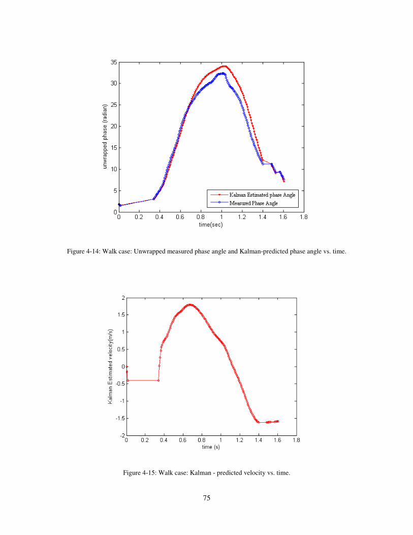
75

Figure 4-14: Walk case: Unwrapped measured phase angle and Kalman-predicted phase angle vs. time.

Figure 4-15: Walk case: Kalman - predicted velocity vs. time.

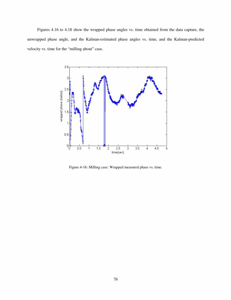
76

Figures 4.16 to 4.18 show the wrapped phase angles vs. time obtained from the data capture, the

unwrapped phase angle, and the Kalman-estimated phase angles vs. time, and the Kalman-predicted

velocity vs. time for the “milling about” case.

Figure 4-16: Milling case: Wrapped measured phase vs. time.

77

Figure 4-17: Milling case: Unwrapped measured phase angle and Kalman-predicted phase angle vs. time.

Figure 4-18: Milling case: Kalman Predicted velocity vs. time

78

Note that the velocity as seen by the reader antenna is not expected to be constant when the tagged

person moves through the portal from one end to the other. This is because the direction in which the

antenna is shining is transverse to the direction of the tagged object’s motion. The velocity is thus a

function of the angle between the direction of the antenna and the line that connects the antenna bore sight

to the current position of the object. If the object were moving at a constant velocity, the velocity

magnitude would be maximum when the object starts from one end of the portal, would decrease as the

tag approaches the antenna bore sight, would become zero when the person is at the centre or directly

along the direction of the antenna bore sight, and then again increases but in the other direction or with an

opposite sign.

As observed from the wrapped phase plot of the “walk case”, i.e., Figure 4.13, the phase vs. time

slope follows a positive trend when the tag approaches the antenna bore sight and changes direction to

follow a negative trend after the tag crosses the antenna bore sight. The Kalman-estimated velocity as

seen in Figure 4.15 starts from zero (which is the initial velocity of the human fed into the algorithm),

continues to increase as it takes some time to reach the maximum value, then follows the trend as

described. In the “milling-about” case, the Kalman-estimated velocity settles to a mean value of about 0

m/s.

If we plot a normalized histogram of velocities for both these cases, where the x-axis represents the

velocity bins with a bin size of 0.2 m/s, they appear as shown in Figure 4-19. This can be used to

differentiate between cases in which a person walks through the portal as opposed to a person who is

standing relatively still. This could be used to alert people who are standing still for a long time, to the

presence of hazardous radiations and for other similar uses.

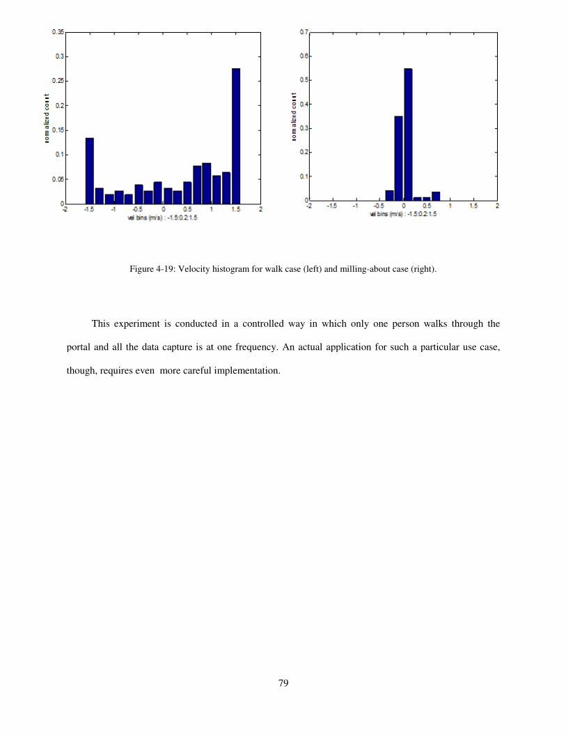
Figure 4-19: Velocity histogram for walk cas

This experiment is conducted in a controlled way in which only one person walks through the

portal and all the data capture is at one frequency. An actual application for such a particular use case,

though, requires even more careful implementation.

79

19: Velocity histogram for walk case (left) and milling-about case (right).

This experiment is conducted in a controlled way in which only one person walks through the

portal and all the data capture is at one frequency. An actual application for such a particular use case,

more careful implementation.

about case (right).

This experiment is conducted in a controlled way in which only one person walks through the

portal and all the data capture is at one frequency. An actual application for such a particular use case,

80

Chapter 5

Summary and Future Work

This thesis has explained tag range and tag motion estimation based on phase information for

passive RFID tags.

Data were collected in different environmental setups for tag range estimation. The tag range data

collected in the chamber has an average range error (standard deviation) of 0.097 m and an average

percentage error of 10.5 as per Table 3-1, and the tag range data collected in open space has an average

range error (standard deviation) of 0.187 m and an average percentage error of 4.3 for setup 1 as per

Table 3-3. Both data sets show that the methods used yield fairly accurate measurements. An overall

accuracy of about 0.305 m or a tag range error below 10 % is likely to be suitable for many applications.

Thus, the accuracy for the anechoic chamber and the particular open-space setup is within desired limits.

However, the data collected in the industrial setting have a much higher average error (standard deviation)

of 1.242 m and percentage error of 26.7 as seen from Table 3.4. Similar to tag range estimation, data for

tag motion estimation were also collected in industrial settings. A real-life use case has been included in

Section 4.5.3 demonstrating the use of the tag motion estimation feature. Despite the multipath present,

the algorithm is quite robust given the application for which it is being used. For the walk case, the

ingress and egress direction of the tag movement and the point at which the tag crosses the antenna bore

sight, i.e., the center point, can be identified. Also, the walk case can be differentiated from the milling-

about case.

An RSSI model developed for the tag range data collected in open space demonstrates the effect of

multipath reflection caused due to the indirect ground-reflected ray. This model also suggests that RSSI

information and phase information can be used together in order to render the tag range and tag motion

estimation algorithm more robust and reliable.

It is clear that performing range and motion estimation of passive tags depends on a number of

factors, the most important being the operating environment. A real challenge is to make the tag range

and motion estimation robust to multipath in indoor and industrial settings in which the multipath sources

81

and locations are unknown. Measures such as avoiding metallic objects in the surrounding area will boost

the performance of the algorithms. In addition, an important next step is to build on this study’s results by

developing a site-survey tool capable of indicating how suitable any particular environment would before

using this feature.

Factors other than the operating environment also affect performance. These factors include the

type of antenna and its characteristics (e.g., dipole or directional), type of tag (semi-passive tags give

much longer read ranges), polarization and orientation of the tag and antenna, placement or height of the

tag and antenna from the ground, number of stray tags in the field, tag detuning effects etc.

This thesis has explained different processing techniques such as end-point regression, linear

regression, periodic functional fit, and Kalman filtering. These techniques should be chosen based on

different application needs. In an algorithmic implementation of tag range and tag motion estimation, the

following factors must be considered: maximum tag range, maximum and minimum tag speed, processing

time, frequency spacing and time spacing, number of data points, processor memory, customer time-out

requirements, etc. A well-implemented algorithm and a correct technique are necessary for tag range and

tag motion estimation to give accurate results.

This study has also explained some ways in which the algorithms could be improved, such as by

interpolating missing phase reads. Future research could consider making the algorithm as dynamic and

real-time as possible, establishing effective frequency-spacing strategies for tag range estimation, and

setting a desired accuracy metric, which if not met would mean no results would be reported.

These observations, then, constitute a summary of this study’s achievements as well as offering

suggestions for meaningful and applications-oriented future research. The concluding section cites some

examples in which the range and motion determination of RFID tags could be used effectively.

82

5.1 Applications

Passive RFID is a low-energy, non-line-of-sight, and comparatively inexpensive technology.

Addition of tag localization and motion estimation capabilities to passive RFID will enable and enhance a

wide range of RFID applications.

Tag range estimation finds several useful applications in supply chain management, such as

inferring the location of tagged objects along with their identity in a storage warehouse. This is likely to

save time spent in looking for a particular item. Other applications include tracking baggage at airport

terminals. In addition, tag range estimation could be used effectively in a smart-house setting to establish

and track the position of people and objects to optimize user interfaces and energy use, as stated in [13].

In tandem with localization information, tag motion estimation can be used to track the motion of

people and objects in order to recognize and model dynamic activities. It has applications in retail

merchandising, such as determining when goods are checked in and out of a warehouse. Similarly, tag

motion estimation—specifically, the RFID’s direction-finding feature—can be used as a security

measure, e.g., monitoring the movement of customers or even staff carrying tagged objects in or out of

the store. Testing the speed limit of cars passing through a toll-booth is another application of tag motion

estimation.

In all the experiments for tag range, a single tag range measurement using a single receiving

antenna has been carried out. This yields the tag range or gives a distance of, for example, “d” between

the RFID tag and the RFID tag reader antenna. The location of the tag can thus be known to lie

approximately on a sphere of radius “d” surrounding the antenna. To determine the precise location in

three dimensions, multiple tag range measurements must be made by displacing the reader antenna. This

is explained in [1]. In some cases, an array of several receiving antennas is used to locate the tag in three

dimensions [25-26].

Similarly, this study has demonstrated tag motion estimation by using only one receiving antenna,

which gives only radial speed and direction. The same protocols can be extended to motion estimation in

three dimensions using suitable techniques.

83

Several other applications similar to those listed here are easy to imagine. It is, therefore, clear that

tag range and tag motion estimation will add significantly to the current advantages of passive RFID

technology and in developing of a Real-Time Location and Tracking System.

84

REFERENCES

[1] Carrick, J.C., et al., “Method and Apparatuses for RFID Tag Range Determination,” US Patent

Application 20100109844 A1, May 6, 2010.

[2] D.M. Dobkin, “A Radio-Oriented Introduction to RFID-Protocols, Tags and Applications,” High

Frequency Electronics Magazine, August 2005, pp. 32-46.

[3] EPC Radio Frequency Identification Protocols Class 1 Generation-2 UHF RFID Protocol for

Communications at 860-960 MHz Version 1.0.9, EPC Global Inc., Dec. 2005.

[4] M. Bouet, A. L. dos Santos, “RFID tags: Positioning principles and localization techniques”, 1st

IFIP Wireless Days, Nov. 2008, pp.1–5.

[5] Feifei, G., Zhang, C., Wang, M., and Xu, X., “Research of indoor location method based on the

RFID technology,” Proceedings of the 11th Joint Conference on Information Sciences, Atlantis

Press: 2008.

[6] Kim, M., and Chong, N., “Direction sensing RFID reader for mobile robot navigation,” IEEE

Transactions on Automation Science and Engineering, vol. 6, no. 1, Jan. 2009, pp. 44–54.

[7] Oikawa, Y., “Tag movement direction estimation methods in an RFID gate system,” 6th

International Symposium on Wireless Communication Systems, Sept. 2009, pp. 41–45.

[8] Hansen, T., and Oristaglio, M., “Method for controlling the angular extent of interrogation zones

in RFID,”IEEE Antennas and Wireless Propagation Letters, vol. 5, no. 1, Dec. 2006, pp. 134–

137.

[9] Chattopadhyay, A., and Harish, A., “Analysis of low range Indoor Location Tracking techniques

using Passive UHF RFID tags,” IEEE Radio and Wireless Symposium, Orlando, FL, Jan. 2008,

pp. 35–54.

[10] Alippi, C., et al., “A statistical approach to localize passive RFIDs,” IEEE International

Symposium on Circuits and Systems, Island of Kos, Greece, Sept. 2006, pp. 843–846.

85

[11] Nikitin, P.V., Martinez, R., Ramamurthy, S., Leland, H., Spiess, G., Rao, K. V. S., “Phase based

spatial identification of UHF RFID tags,” Proc. of the IEEE International Conference on RFID,

Apr. 2010.

[12] Li X., Zhang Y., Amin M., “Multifrequency-based range estimation of RFID Tags,” IEEE RFID

Conference, April 2009, pp. 147–154.

[13] Arnitz D., Witrisal K., Muehlmann U., “Multifrequency Continuous-Wave Radar Approach to

Ranging in Passive UHF RFID,” IEEE Transactions on MTT, vol. 57, no. 5, May 2009, pp. 1398–

1405.

[14] Hekimian-Williams, C., Grant, B., Liu, X., Zhang, Z., and Kumar P., “Accurate localization of

RFID tags using phase difference,” IEEE International Conference on RFID, April 2010.

[15] Amin M., Zemany, Setlur P., and Ahmad F., “Moving target localization for indoor imaging using

dual frequency CW radars,” 2006 IEEE Sensor Array and Multichannel Signal Processing

Workshop (IEEE Cat. No.06EX1345C), 2006, pp. 367–71.

[16] Bridgelall R., et al., “Object Location System and Method Using RFID,” US Patent No. US

7119738 B2, Oct 10, 2010.

[17] Rappaport, T., “Mobile Radio Propagation: Large-Scale Path Loss” in Wireless Communications:

Principles and Practice, 2nd ed., New Jersey: Prentice-Hall. PTR, 1996.

[18] Dobkin, D., “Radio Basic for UHF RFID” in The RF in RFID: Passive UHF RFID in practice,

MA: Elsevier Inc., 2008.

[19] Rappaport, T., “Characterization of UHF multipath radio channels in factory buildings,” IEEE

Transactions on Antennas and Propagation, vol. 37, no.8, Aug. 1989, pp.1058-1069.

[20] Seidel, S., and Rappaport, T., “914 MHz path loss prediction models for indoor wireless

communications in multifloored buildings,” IEEE Transactions on Antennas and Propagation,

vol. 40, no. 2, Feb. 1992, pp. 207-217.

[21] Barton, D.K., and Leonov, S.A., “Radar technology encyclopedia”, Artech House Inc, 1997.

86

[22] Kvaksrud,T-I, “Range measurements in an open field environment”, Design Note DN018, Texas

Instruments.

[23] Boccadoro, M., and Martinelli, F., and Pagnottelli, S., “Constrained and quantized Kalman

filtering for an RFID robot localization problem,” Auton Robot, vol. 29, pp. 235–251, June 2010.

[24] Welch, G., and Bishop, G., “An introduction to the Kalman filter,” TR95-041, Dept. of Computer

Science, University of North Carolina at Chapel Hill, NC, USA, 2004.

[25] Zhang, Y., Amin, M., and Kaushik, S., “Localization and tracking of passive RFID tags based on

direction estimation,” International Journal of Antennas and Propagation, pp. 1–9, Oct. 2007.

[26] Wang, J., Amin, M., and Zhang, Y., “Signal and array processing techniques for RFID readers,”

Proceedings of the SPIE, vol. 6248, 2006.