
Technical Addendum to the Winningsplan Groningen 2016 ...
163
1 Technical Addendum to the Winningsplan 2016 – 1 st April 2016 Technical Addendum to the Winningsplan Groningen 2016 Production, Subsidence, Induced Earthquakes and Seismic Hazard and Risk Assessment in the Groningen Field Part I Summary & Production
Transcript of Technical Addendum to the Winningsplan Groningen 2016 ...
1
Technical Addendum to the Winningsplan 2016 – 1st April 2016
Technical Addendum to the Winningsplan Groningen 2016 Production, Subsidence, Induced Earthquakes and Seismic Hazard and Risk Assessment in the Groningen Field Part I Summary & Production

2
Technical Addendum to the Winningsplan 2016 – 1st April 2016
The report “Technical Addendum to the Winningsplan Groningen 2016 - Production, Subsidence, Induced Earthquakes and Seismic Hazard and Risk Assessment in the Groningen Field” consists of five separate documents:
Document 1 Chapters 1 to 5; Summary and Production
Document 2 Chapter 6; Subsidence
Document 3 Chapter 7; Hazard
Document 4 Chapter 8; Risk
Document 5 Chapter 9; Damage and Appendices.
Each of these documents is also available as a *.pdf file of a size smaller than 10Mbyte, allowing sharing through e-mail.
© EP201603238413 Dit rapport is een weerslag van een voortdurend studie- en dataverzamelingsprogramma en bevat de stand der kennis van april 2016. Het copyright van dit rapport ligt bij de Nederlandse Aardolie Maatschappij B.V. Het copyright van de onderliggende studies berust bij de respectievelijke auteurs. Dit rapport of delen daaruit mogen alleen met een nadrukkelijke status-en bronvermelding worden overgenomen of gepubliceerd.
3
Technical Addendum to the Winningsplan 2016 – 1st April 2016
Contents Samenvatting ................................................................................................................................................ 5
Achtergrond bij deze technische bijlage ................................................................................................... 5
Conclusies ................................................................................................................................................. 5
Productie 5
Bodemdaling 5
Seismiciteit 5
Seismische dreiging 6
Seismische risico 7
Schade 10
Management Summary .............................................................................................................................. 12
Background to this Report 12
Conclusions 12
1 Introduction ........................................................................................................................................ 18
2 Static and dynamic model update ...................................................................................................... 19
2.1 Introduction ................................................................................................................................ 19
2.2 What is new in GFR2015 ............................................................................................................. 19
2.3 Dynamic model update since November 2015 HRA ................................................................... 22
2.4 Dynamic Compartments and Initialization ................................................................................. 23
2.5 History matching workflow ......................................................................................................... 25
2.6 History matching results ............................................................................................................. 28
2.7 Uncertainty analysis workflow and results ................................................................................. 29
3 The Groningen System ........................................................................................................................ 32
3.1 Gas Production System ............................................................................................................... 32
3.2 Operational constraints .............................................................................................................. 33
3.2.1 UGS injection requirements 34
3.2.2 Minimum flow 34
4 Reduction of seismic risk through production management ............................................................. 35
4.1 Introduction ................................................................................................................................ 35
4.2 Hazard and Risk Assessment – Interim update November 2015 ................................................ 35
4.2.1 January 2015 regions 35
4.2.2 Pressure response driven by January 2015 regions 36
4.2.3 Observations from Nov 2015 HRA 38
4.3 Optimisation of the production distribution .............................................................................. 41

4
Technical Addendum to the Winningsplan 2016 – 1st April 2016
4.3.1 Considerations 41
4.3.2 New areas 43
5 Forecasting with the optimised production distribution .................................................................... 45
5.1 Introduction ................................................................................................................................ 45
5.2 Annual Demand profile ............................................................................................................... 45
5.3 Capacity ....................................................................................................................................... 45
5.4 Production logic .......................................................................................................................... 45
5.5 Production Scenarios .................................................................................................................. 45
Appendix Introduction to the Geology of the Groningen field (Static Model Description) ................ 51
Structural setting 51
Stratigraphy and depositional setting 53
Reservoir model and rock properties 55
5
Technical Addendum to the Winningsplan 2016 – 1st April 2016
Samenvatting Achtergrond bij deze technische bijlage Op 1 april 2016 heeft de NAM het Winningsplan Groningen Gasveld 2016 ingediend bij de Minister van Economische Zaken (EZ). Dit Winningsplan gaat vergezeld met een Technische Bijlage C, waarin technische verdieping en achtergronden zijn gegeven ten behoeve van het Winningsplan.
Deze bijlage presenteert diverse scenario’s voor de productie van gas uit het Groningen gasveld en geeft de beoordeling van de effecten van elk van deze scenario’s in termen van bodemdaling en geïnduceerde seismiciteit. Voor elk scenario worden de dreiging (‘hazard’) en de risico’s (‘risks’) inclusief het schadepotentieel beoordeeld en daaromtrent verwachtingen gegeven.
Conclusies
Productie De productiescenario’s beslaan drie niveaus: 21 miljard m
3 (bcm) per jaar, 27 miljard m
3 (bcm) per jaar en 33
miljard m3 (bcm) per jaar. Vervolgens wordt voor elk productieniveau een tweetal verdelingen over het
gasveld gehanteerd: in aanvulling op de distributie van de winning over het gasveld zoals doorgevoerd op basis van het instemmingsbesluit van EZ van januari 2014 is een geoptimaliseerd scenario ontwikkeld. Deze optimalisatieoptie van de winning over het veld richt zich op de beperking van de seimiciteit. In totaal leidt dit tot een zestal beoordeelde scenario’s.
Met de mogelijke optimalisatie van de productieverdeling wordt tevens een andere clustering en regionalisatie van winningslocaties geïntroduceerd, inclusief bijpassende productieplafonds. In totaliteit blijft de productie voldoen aan de generieke beperkingen van productie uit het gehele gasveld.
De beschikbare statische en dynamische modellen van het Groningen gasveld zijn verder verfijnd; suggesties gedaan door SGS Horizon (een onafhankelijk instituut dat toeziet op reserves binnen de olie- en gasindustrie), TNO en het Staatstoezicht op de Mijnen (SodM) zijn meegenomen in de aanpassingen. Het nieuwe reservoirmodel is nu niet alleen gekalibreerd op basis van de feitelijke, historische metingen (‘history match’) van productievolumes, reservoirdrukken en aquifers,maar ook bodemdaling.
Bodemdaling De meting van bodemdaling heeft plaats sinds het begin van de productie van aardgas in Groningen. Onder
meer de volgende meettechnieken worden daarbij toegepast: waterpasmetingen en metingen met behulp van satellieten (InSAR en GPS).
Zowel het gehanteerde 'Time decay model’ als het ‘Rate Type Compaction isotach Model’ (RTCiM) voor de compactie geven een goede passing met de gemeten bodemdaling boven het gasveld.
De waargenomen bodemdaling in het centrum van de bodemdalingsschotel was circa 33 centimeter in 2013. De verwachting is dat daar de daling na afloop van de productie ongeveer 50 centimeter zal zijn.
Het RTCiM-model is verkozen als het basismodel voor de compactie, omdat deze de beste overeenkomsten in tijd en ruimte geeft met de waargenomen reactie van bodemdaling op veranderingen in productie.
Seismiciteit Voor de periode van 2016 tot 2021 zal de gemiddelde hoeveelheid aardbevingen en de gemiddelde energie die daarbij vrij zal komen – voor alle productiescenario’s – naar verwachting van dezelfde orde zijn als in de periode van 2012 tot 2015.
6
Technical Addendum to the Winningsplan 2016 – 1st April 2016
Seismische dreiging De effecten van de lokale, ondiepe bodemsamenstelling op de grondbeweging bij een aardbeving zijn nu
onderdeel van de analyse. In de voorliggende analyse is een correctie doorgevoerd in de software die gebruikt wordt om de
bodembeweging te voorspellen. Deze omissie is recent ontdekt tijdens een detail-analyse en vergelijking van een tweetal modellen die worden gebruikt voor een parallelle berekening van de dreiging en risico’s. De correctie is besproken met onder meer het KNMI, TNO, SodM en de Scientific Adisory Committee (SAC) die namens EZ toeziet op de kwaliteit van de risicobeoordeling. De waarde voor de variatie in lokale bodemsamenstelling, die werd gebruikt in het model dat ten grondslag lag aan de Hazard and Risk Assessment (HRA) van november 2015, was abusievelijk ingesteld op de maximale waarde. Dit onafhankelijk van de verwachte beweging van de diepere ondergrond, terwijl deze waarde variabel moet zijn aan de verwachte sterkte van aardbevingen. De doorgevoerde correctie heeft er toe geleid, dat zowel de seismische dreiging als het seismische risico in de onderhavige Technische Bijlage lager zijn dan in de HRA van november 2015.
Het onderzoek en de beslisstructuur/-boom door middels van zogeheten ‘logic tree’ omvat de meest significante onzekerheden. Het gewicht dat is toegekend aan deze onzekerheden is aangepast in overeenstemming met de verwachtingen die van overheidszijde zijn aangegeven (EZ’s verwachtingenbrief van 15 februari 2016).
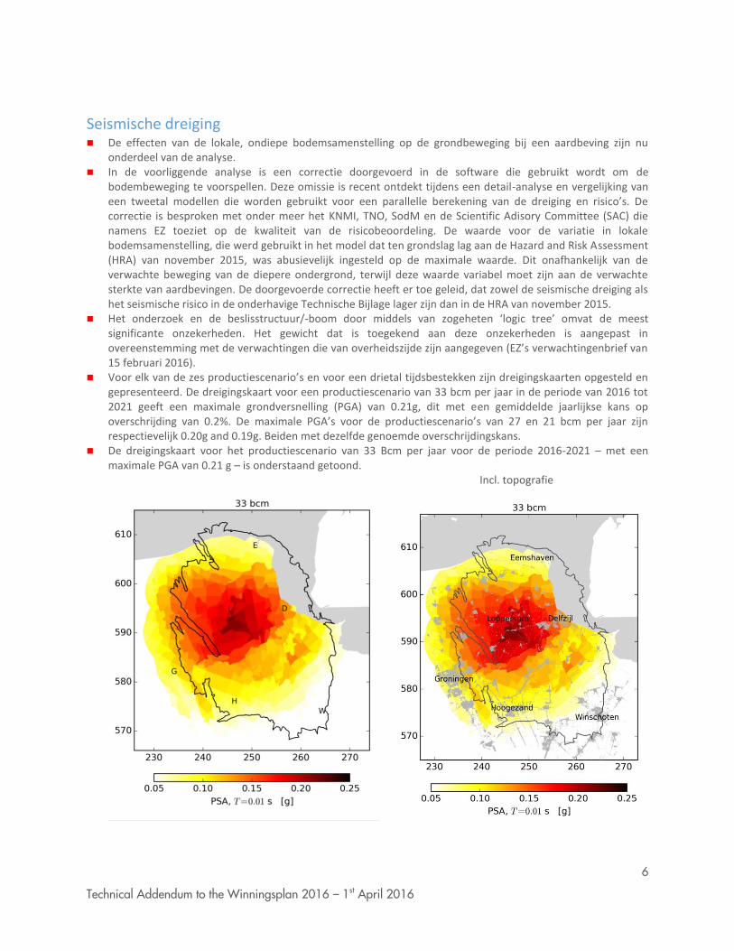
Voor elk van de zes productiescenario’s en voor een drietal tijdsbestekken zijn dreigingskaarten opgesteld en gepresenteerd. De dreigingskaart voor een productiescenario van 33 bcm per jaar in de periode van 2016 tot 2021 geeft een maximale grondversnelling (PGA) van 0.21g, dit met een gemiddelde jaarlijkse kans op overschrijding van 0.2%. De maximale PGA’s voor de productiescenario’s van 27 en 21 bcm per jaar zijn respectievelijk 0.20g and 0.19g. Beiden met dezelfde genoemde overschrijdingskans.
De dreigingskaart voor het productiescenario van 33 Bcm per jaar voor de periode 2016-2021 – met een maximale PGA van 0.21 g – is onderstaand getoond. Incl. topografie

7
Technical Addendum to the Winningsplan 2016 – 1st April 2016
Om aan te tonen welke aardbevingen de grootste bijdrage leveren aan de seismische dreiging is een onderscheid gemaakt naar een tweetal gebieden; het gebied rond Loppersum en de Stad Groningen. Wanneer wordt gekeken naar het Loppersum-gebied, blijkt dat de grootste bijdrage aan de seismische dreiging in dat gebied komt van aardbevingen binnen hetzelfde gebied (aardbevingen binnen een afstand van minder dan 5 kilometer en met een magnitude tussen de 4 en 5). Dit in tegenstelling tot de dreiging voor de Stad Groningen, die met name wordt gevormd door aardbevingen met een epicentrum die op ongeveer 10 kilometer afstand ligt, in de richting van Loppersum. Aardbevingen op grotere afstanden van de Stad zouden ook significante grondbewegingen in de Stad kunnen veroorzaken, maar deze moeten dan wel van een zwaardere magnitude zijn.
Seismische risico De risico-analyse omvat het bezwijken van gebouwen, met een focus op constructieve elementen van een
bouwwwerk. Potentieel vallende, niet-constructieve objecten zijn beoordeeld volgens een aparte methodiek en beschreven in een afzonderlijk rapport.
De beoordeling van het individueel risico (op basis van ILPR, Inside Local Personal Risk) van bewoners in de regio toont, dat geen van de bewoners wordt blootgesteld aan een risico groter dan 10
-4 per jaar in de periode
van 2016 tot 2021. Geïllustreerd in onderstaande grafieken zijn er enkele honderden gebouwen waarin de bewoners mogelijk zijn blootgesteld aan een risico dat ligt tussen de 10
-4 en 10
-5 per jaar voor de genoemde
perdiode.
LPR Assessment for the 33 Bcm/year Scenario
De norm voor veiligheid die het Ministerie van EZ op basis van de adviezen van de Commissie Meijdam heeft gesteld kan worden behaald door het voorziene programma van bouwkundig versterken uit te voeren. Hierdoor kunnen alle betreffende gebouwen in een periode van 5 jaar worden verstrekt tot (onder) het risiconiveau van 10
-5. Op basis van de huidige onzekerheden (gereflecteerd in de bandbreedte) geldt voor
ongeveer duizend gebouwen, dat er een kans van meer dan 10% bestaat dat de bewoners blootgesteld zijn aan een risico tussen de 10
-4 en 10
-5.
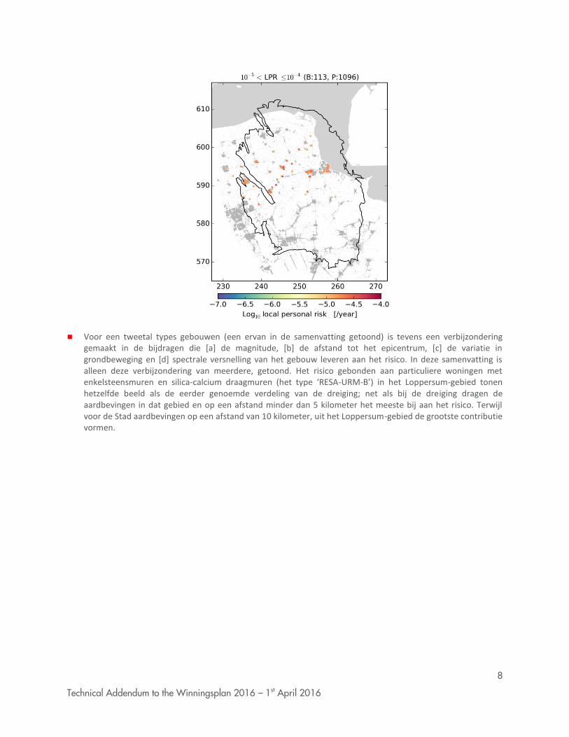
De gebouwen met een risico tussen de 10-4
en 10-5
per jaar bevinden zich met name op de lijn die zich uitstrekt van Delfzijl, via Loppersum, naar Bedum. In de onderstaande figuur zijn deze door middel van een kleuring gevisualiseerd.
8
Technical Addendum to the Winningsplan 2016 – 1st April 2016
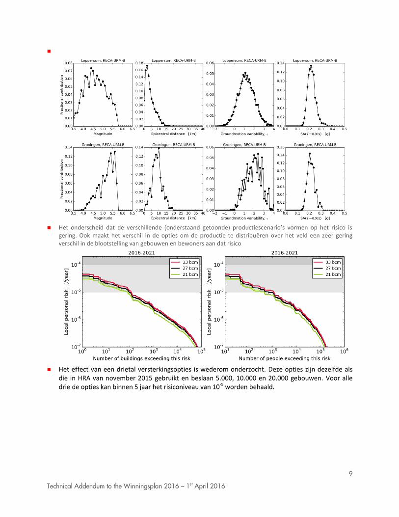
Voor een tweetal types gebouwen (een ervan in de samenvatting getoond) is tevens een verbijzondering
gemaakt in de bijdragen die [a] de magnitude, [b] de afstand tot het epicentrum, [c] de variatie in grondbeweging en [d] spectrale versnelling van het gebouw leveren aan het risico. In deze samenvatting is alleen deze verbijzondering van meerdere, getoond. Het risico gebonden aan particuliere woningen met enkelsteensmuren en silica-calcium draagmuren (het type ‘RESA-URM-B’) in het Loppersum-gebied tonen hetzelfde beeld als de eerder genoemde verdeling van de dreiging; net als bij de dreiging dragen de aardbevingen in dat gebied en op een afstand minder dan 5 kilometer het meeste bij aan het risico. Terwijl voor de Stad aardbevingen op een afstand van 10 kilometer, uit het Loppersum-gebied de grootste contributie vormen.
9
Technical Addendum to the Winningsplan 2016 – 1st April 2016
Het onderscheid dat de verschillende (onderstaand getoonde) productiescenario’s vormen op het risico is
gering. Ook maakt het verschil in de opties om de productie te distribuëren over het veld een zeer gering verschil in de blootstelling van gebouwen en bewoners aan dat risico
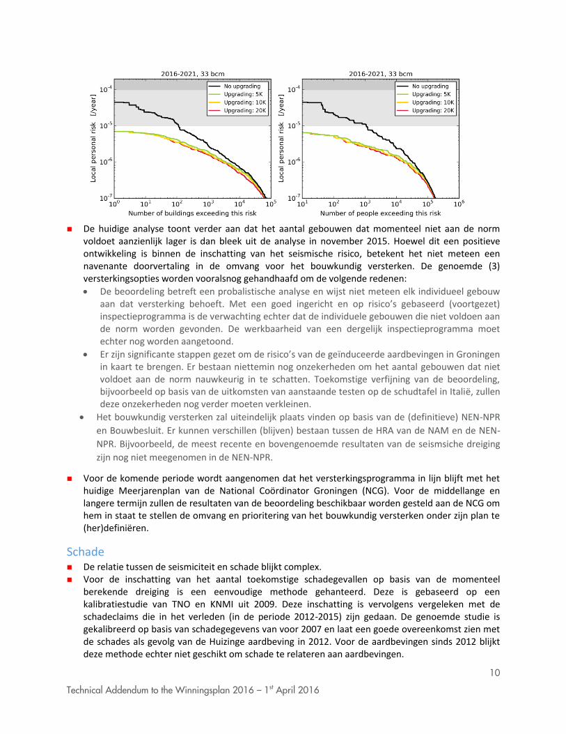
Het effect van een drietal versterkingsopties is wederom onderzocht. Deze opties zijn dezelfde als
die in HRA van november 2015 gebruikt en beslaan 5.000, 10.000 en 20.000 gebouwen. Voor alle drie de opties kan binnen 5 jaar het risiconiveau van 10-5 worden behaald.
10
Technical Addendum to the Winningsplan 2016 – 1st April 2016
De huidige analyse toont verder aan dat het aantal gebouwen dat momenteel niet aan de norm
voldoet aanzienlijk lager is dan bleek uit de analyse in november 2015. Hoewel dit een positieve ontwikkeling is binnen de inschatting van het seismische risico, betekent het niet meteen een navenante doorvertaling in de omvang voor het bouwkundig versterken. De genoemde (3) versterkingsopties worden vooralsnog gehandhaafd om de volgende redenen:
De beoordeling betreft een probalistische analyse en wijst niet meteen elk individueel gebouw aan dat versterking behoeft. Met een goed ingericht en op risico’s gebaseerd (voortgezet) inspectieprogramma is de verwachting echter dat de individuele gebouwen die niet voldoen aan de norm worden gevonden. De werkbaarheid van een dergelijk inspectieprogramma moet echter nog worden aangetoond.
Er zijn significante stappen gezet om de risico’s van de geïnduceerde aardbevingen in Groningen in kaart te brengen. Er bestaan niettemin nog onzekerheden om het aantal gebouwen dat niet voldoet aan de norm nauwkeurig in te schatten. Toekomstige verfijning van de beoordeling, bijvoorbeeld op basis van de uitkomsten van aanstaande testen op de schudtafel in Italië, zullen deze onzekerheden nog verder moeten verkleinen.
Het bouwkundig versterken zal uiteindelijk plaats vinden op basis van de (definitieve) NEN-NPR
en Bouwbesluit. Er kunnen verschillen (blijven) bestaan tussen de HRA van de NAM en de NEN-
NPR. Bijvoorbeeld, de meest recente en bovengenoemde resultaten van de seismsiche dreiging
zijn nog niet meegenomen in de NEN-NPR.
Voor de komende periode wordt aangenomen dat het versterkingsprogramma in lijn blijft met het huidige Meerjarenplan van de National Coördinator Groningen (NCG). Voor de middellange en langere termijn zullen de resultaten van de beoordeling beschikbaar worden gesteld aan de NCG om hem in staat te stellen de omvang en prioritering van het bouwkundig versterken onder zijn plan te (her)definiëren.
Schade De relatie tussen de seismiciteit en schade blijkt complex. Voor de inschatting van het aantal toekomstige schadegevallen op basis van de momenteel
berekende dreiging is een eenvoudige methode gehanteerd. Deze is gebaseerd op een kalibratiestudie van TNO en KNMI uit 2009. Deze inschatting is vervolgens vergeleken met de schadeclaims die in het verleden (in de periode 2012-2015) zijn gedaan. De genoemde studie is gekalibreerd op basis van schadegegevens van voor 2007 en laat een goede overeenkomst zien met de schades als gevolg van de Huizinge aardbeving in 2012. Voor de aardbevingen sinds 2012 blijkt deze methode echter niet geschikt om schade te relateren aan aardbevingen.
11
Technical Addendum to the Winningsplan 2016 – 1st April 2016
De schade-gegevens wijzen naar een verhoogd, maar nog niet verklaard, aantal schadeclaims na de Huizinge aardbeving.
Nadere studie is nodig naar:
De gebieden waar de aardbevingen een dusdanige energie kunnen genereren dat er schade ontstaat.
De precieze relatie tussen de schadeclaims (en rapportage daarvan) en de actuele schade.
De wijze waarop schades als A, B en C (al dan niet aardbevingsgerelateerd, of een combinatie daarvan) wordt geclassificeerd.
Er lijkt een opwaartse trend te zijn ontstaan binnen het aandeel C-schades (schades die niet toegewezen kunnen worden aan aardbevingen) sinds medio 2015.
De geïnstalleerde TNO-sensoren tonen dat gebouwen in de regio trillingen vertonen als gevolg van een diversiteit aan oorzaken, variërend van aardbevingen tot verkeer en bouwwerkzaamheden.
12
Technical Addendum to the Winningsplan 2016 – 1st April 2016
Management Summary
Background to this Report On the 1
st April 2016 NAM submitted the Groningen Winningsplan 2016 to the Minister of Economic Affairs. This
Winningsplan is accompanied with a Technical Addendum providing further background to the technical assessments used in the Winningsplan.
This addendum presents scenarios for the gas production from the reservoir and an updated assessment of the consequences of the production for each scenario in terms of subsidence and induced seismicity. For each scenario, the hazard and risk (including damage) resulting from induced seismicity are assessed and forecasts are presented.
Conclusions
Production
The gas production scenarios cover three annual production levels for the field: 21 Bcm/annum, 27 Bcm/annum and 33 Bcm/annum. Furthermore, for each production level, two different distributions of the offtake from the field are used. This is in addition to the distribution of the offtake over the field as imposed by the Ministerial decision of January 2014 an optimized scenario was developed. The further optimization of the distributions of the offtake over the field aims to minimize risk. This results in a total of six scenarios.
The optimized field offtake introduces an alternative grouping of the production clusters and their production limits. The gas production scenarios adhere to the limitation of the Groningen production system.
The static and dynamic reservoir models of the Groningen field have been further updated. Comments from a previous review of the model for Winningsplan 2013 by SGS Horizon (independent reserves auditor), and by TNO-AGE and SodM have been incorporated. The new reservoir model is now history matched with production data, measured reservoir pressures, data of water rise from the aquifer and subsidence data.
Subsidence
Subsidence monitoring in Groningen is in place since the start of production. The following surveying techniques are applied: Spirit levelling, PS-InSAR (Satellite Radar Interferometry) and GPS.
Both the Time decay and the RTCiM (Rate Type Compaction isotach Model) compaction models result in a good overall fit to the observed subsidence data above the Groningen field.
The RTCiM compaction model is chosen as the base case compaction model because it results in the best fit to the temporal and spatial observed response of the subsidence to production changes.
Maximum observed subsidence above the center of the field was around 33 cm in 2013. The forecasted maximum subsidence at the end of field life is approximately 50 cm.
Seismic Event Rate
For the period 2016 to 2021, both the median annual total seismic event rate and median annual seismic moments are, for all of the volume cases, forecasted to remain in a similar range as the actual seismic event rate and moment observed in the period 2012 – 2015.
Seismic Hazard
The effects of the local soil conditions on the ground movement response to an earthquake have been incorporated in the hazard assessment.
In the current hazard assessment an error in the software implementation of the model for ground motion prediction has been corrected. This was recently detected by a detailed comparison of hazard and risk results obtained from two independent software implementations and has been discussed with KNMI, TNO, SodM and SAC. As a result of this mistake in the interim update of the hazard and risk assessment of November 2015, the variability in the local site response was effectively set to its maximum value irrespective of the level of shaking expected in the underlying rock, whereas this variability should increase with the strength of
13
Technical Addendum to the Winningsplan 2016 – 1st April 2016
shaking. Correcting this mistake has resulted in a lower assessment of the probabilistic hazard and risk in the current Technical Addendum than in the interim update of the hazard and risk assessment of November 2015.
The logic tree capturing the main uncertainty scenarios and their weights has been updated in line with the guidance in the expectation letter (verwachtingenbrief) of 15 February 2016.
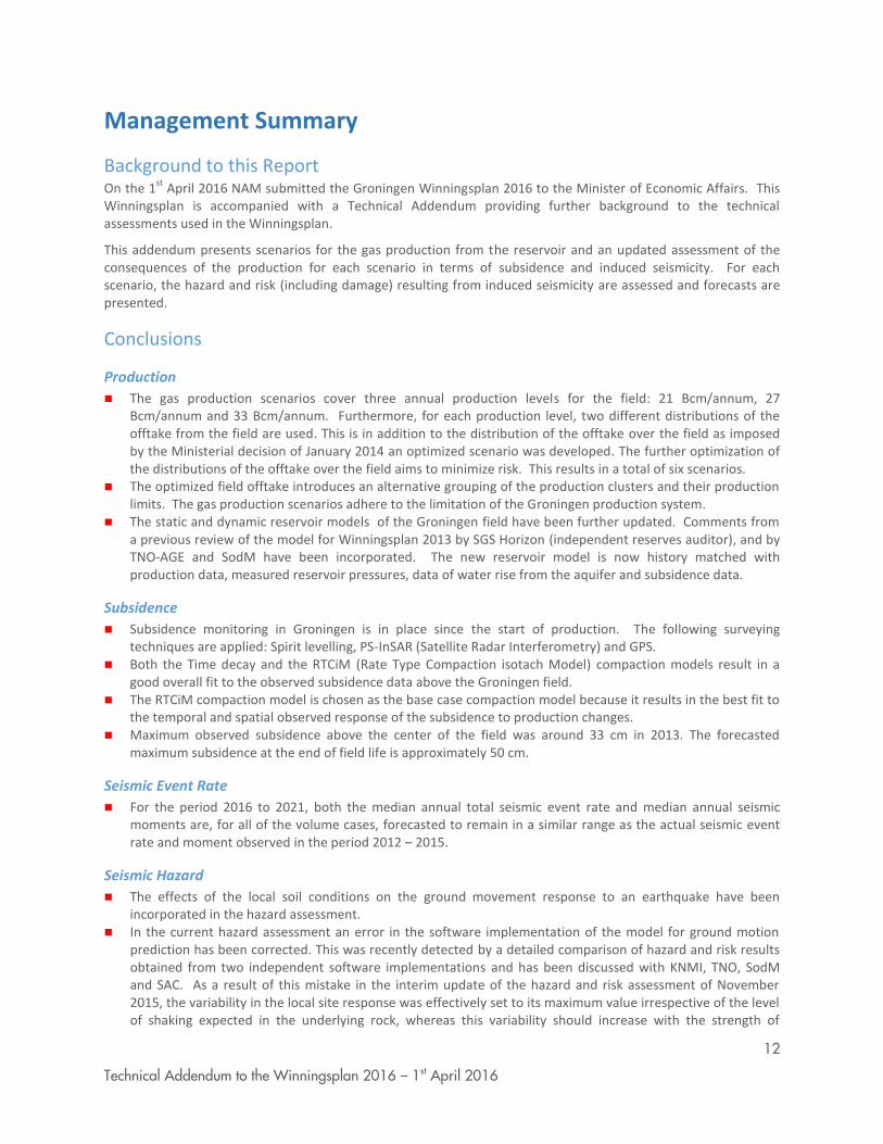
A Hazard Map is presented for each of the six production scenarios for three time periods. The hazard map for the production scenario of 33 Bcm/annum shows for the period 2016 to 2021 a maximum PGA of 0.21g with an average 0.2% annual chance of exceedance. The maximum PGA for the production scenario of 27 Bcm/annum and 21 Bcm/annum are 0.20g and 0.19g respectively with an average 0.2% annual chance of exceedance.
The Hazard Map for the production scenario of 33 Bcm/annum for the period 2016 to 2021 with a maximum PGA of 0.21 g is shown below, where PGA is equal to the PSA for T=0.01 s. Incl. topography
To show which earthquakes have highest impact on the hazard assessment, a disaggregation of the hazard was performed for two areas; Loppersum and Groningen city. The disaggregation for the Loppersum area shows that the largest contribution to the hazard is from earthquakes within the Loppersum area (distance less than 5 km with a magnitude ranging from 4 to 5). In contrast the largest contribution to the hazard in the Groningen city is from earthquakes with an epicenter approximately 10 km away from the city (towards the Loppersum area). The earthquakes located further away can also cause significant ground acceleration in the city of Groningen, but need to have a larger magnitude.
Seismic Risk
The scope of this risk assessment covers building collapse risk (focused on the structural elements of buildings). Falling object risk (non-structural elements) is assessed through a separate methodology and described in a separate report.
The assessment of ILPR (Inside Local Personal Risk) shows there are no buildings where the inhabitants are
exposed to a mean ILPR in excess of 10-4
/annum for the period 2016 to 2021. There are some 100 buildings
where the inhabitants are exposed to a mean ILPR between 10-4
/annum and 10-5
/annum for the same period.

14
Technical Addendum to the Winningsplan 2016 – 1st April 2016
LPR Assessment for the 33 Bcm/year Scenario
The safety norm for LPR as set by the Minister based on the advice of the Meijdam Committee will be met by executing a structural upgrading program to ensure that inhabitants of all buildings are exposed to a LPR below 10
-5/annum within 5 years. Based on the current uncertainties, for some 1,000 buildings there is a
more than 10% chance that the inhabitants are exposed to an ILPR between 10-4
/annum and 10-5
/annum. The buildings with an ILPR between 10
-4/annum and 10
-5/annum are located primarily in a zone from Delfzijl –
Loppersum – Bedum. Values in the figure have been clipped for this range.
For two building typologies a disaggregation was also performed for contributions to the base-case ILPR for
magnitude, distance from the epicentre, ground motion variability measure, and spectral acceleration causing building collapse. In this summary, only the disaggregation is shown. The ILPR disaggregation results for the residential apartment buildings of unreinforced masonry with silica-calcium load bearing walls (type B) in the Loppersum area (typology RESA-URM-B) show results similar to the disaggregation of the hazard.

15
Technical Addendum to the Winningsplan 2016 – 1st April 2016
As for hazard, earthquakes in the Loppersum area (i.e. at epicentral distances less than 5 km) contribute most to the risk for this area, while for Groningen city, earthquakes at an epicentral distance of 10 km (i.e. in the Loppersum area) are the most important contribution.
The sensitivity of the number of houses with an ILPR between 10-4
/annum and 10-5
/annum to changes in the production level is small. The difference in number of buildings or people exposed to a LPR between the two options for distribution of the production over the field is very small.
The impact of three structural upgrading programs has also been investigated. The programs are the same as
used in November 2015 and target 5,000, 10,000 and 20,000 buildings. All three programs yield a safety level where all buildings reach an ILPR below 10
-5/annum within 5 years.

16
Technical Addendum to the Winningsplan 2016 – 1st April 2016
The current risk assessment indicates that the number of buildings that do not meet the norm of 10
-5/year for
ILPR (~100 buildings) may be considerably lower than the estimate in the previous interim update assessment
of November 2015. While this is good news in terms of the seismic risk in Groningen, it does not immediately
translate into a smaller structural strengthening scope. Consequently, the three structural upgrading scenarios
used for the November 2015 interim update have been retained for this risk assessment. There are three main
reasons for this:
o This is a probabilistic assessment and does not directly indicate each individual building that needs to
be upgraded. In time, with a well-designed and risk-based inspection program it is expected that
individual buildings with ILPR >10-5
can be found with reasonable efficiency, however this efficiency
has not yet been proven.
o Significant progress has been made towards assessing the risk from Groningen earthquakes, however
considerable uncertainty remains in the estimate of the number of buildings that do not meet the
norm based on mean ILPR >10-5
. Future updates of the risk assessment could result in a different
mean value of the risk, such as when new shake table tests are taken into account.
o Ultimately the structural upgrading scope will be based on the NEN-NPR building code, and
differences may exist between this code and the NAM hazard and risk assessment. For example the
latest results for the seismic hazard have not yet been adopted in the NEN-NPR.
In the short-term, the structural upgrading program is expected to be in line with the current plan of the
National Coordinator Groningen (NCG). For the medium to long-term, the results of this risk assessment will
be available to help NCG define the scope and prioritisation of the structural upgrading program.
Damage
A simple forecasting method for D1 damage state, based on the 2009 Kalibratiestudie by TNO/KNMI, was used
to forecast the chance of damage based on hazard data. These forecasts were compared with historical
damage claim data (period 2012- 2015). This study is calibrated on damage data from before 2007 and also
provides good results for building damage (claims) for the Huizinge 2012 earthquake. However, for
earthquakes after 2012, this method is not able to match building damage claims.
The relationship between seismic activity and damage claims appears to be complex.
Empirical evidence pointing to strong increase in the number of claims post-Huizinge (early-2013).
Further research is required into:
o The area where earthquakes could release sufficient energy to cause damage
o the precise relationship between damage claim reports and actual damage
o The assessment of claimed damages as A-, B- or C-damage, or combinations thereof
There appears to be a growing trend in the content of C-damage (damage which cannot be attributed to
earthquakes) in damage claims from mid-2015 onwards.

17
Technical Addendum to the Winningsplan 2016 – 1st April 2016
The TNO sensors show that buildings in Groningen experience accelerations due to a wide variety of causes.
Traffic and construction work also cause building acceleration.

18
Technical Addendum to the Winningsplan 2016 – 1st April 2016
1 Introduction This report provides technical support to the Winningsplan 2016 and consist of the following sections:
1. Introduction
2. Static and dynamic model update
3. The Groningen production system,
4. Reduction of seismic risk through production management,
5. Forecasting with optimized production distributon,
6. Subsidence,
7. Hazard assessment,
8. Risk assessment,
9. Building damage.
The assessment of hazard and risk in the Winningsplan 2016 is based on technical studies for the “Hazard and Risk Assessment - Interim Update November 2015”. The sections on hazard and risk assessment in this Technical Addendum should be read in conjunction with the “Hazard and Risk Assessment - Interim Update November 2015”.
To enable a critical review of this addendum it is presented in English. The conclusions however are summarized in the Dutch summary and in the main text of the Winningsplan 2016, which is prepared in Dutch.

19
Technical Addendum to the Winningsplan 2016 – 1st April 2016
2 Static and dynamic model update 2.1 Introduction This section of the report describes the updates to the reservoir model of the Groningen field since Winningsplan 2013. Emphasis is on the latest updates.
For the Technical Addendum to the Winningsplan Groningen 2013, two subsurface realisations of the Groningen field were used. These models were labelled as G1 and G2:
The G2 model (base case) was the best history matched dynamic model with respect to the reservoir
pressure data (SPTG and RFT) and gas-water contact movement (PNL logs). An update of this G2 model
(GFR2013) has been used for business planning and reserves reporting purposes. The G2 model assumed
weak aquifer support to the north and had a mismatch with subsidence data in the north-western part of
the model area.
An alternative G1 realization had moderately strong aquifer support to the north and showed improved
subsidence match but with less good match to gas-water contact movement.
In support of the WP2016 update, a new Groningen field review was started in 2015. The main reasons for initiating the Groningen Field Review 2015 (GFR2015) and thus replacing the existing models are:
To incorporate new data, insights and modelling approaches.
The need for a single dynamic model that matches pressure and water contact movement, but also
Groningen subsidence data.
Larger model area to allow for improved pressure and subsidence prediction to the west of the field,
including the city of Groningen.
Local reservoir pressure matches (at the cluster level) should be improved to ensure good well capacity
prediction (gas rate vs. tubing-head pressure).
Aquifer behaviour resulting in water rise was not adequately well matched.
New data have been acquired since the last model update.
In addition to the reasons above, a number of comments and recommendations resulting from reviews of the previous static and dynamic model by TNO and SGS Horizon have now been incorporated.
The primary objectives for the updated static and dynamic model are usage in:
Winningsplan 2016
the Seismic Hazard and Risk Assessment process
Secondary objectives include:
Business planning process
Annual Reporting of Petroleum Resources (ARPR)
Identification and maturation of development opportunities
2.2 What is new in GFR2015 The conceptual geological concepts that form the framework for the Groningen subsurface models have not been changed. They are described in an introduction to the geology of the Groningen Field area which is attached to this document for reference (Appendix). The main changes to the static reservoir model include:
The model grid area has been extended approximately 8-10 km to the West and 5 km to the South (Figure 2.1) because:
o The previous model was mainly focused on the Groningen closure since the objectives of the model were different. However, for geomechanical studies like prediction of subsidence, the area outside of the Groningen closure is also of importance.

20
Technical Addendum to the Winningsplan 2016 – 1st April 2016
o Subsidence in the greater Groningen area, including the city of Groningen, is not only affected by pressure depletion in the main Groningen gas field, but also by pressure depletion in adjacent aquifers and surrounding small fields. To improve the forecast of subsidence in this extended area, an expanded larger subsurface model area is required.
o Historical and forecasted pressure values for the extended numerical grid provide a better physical basis for geomechanical calculations. In the previous model pressures in the aquifer were modelled using analytical correlations.
The model grid has been optimized ; o Locally, fault connections have been simplified and small faults have been switched off to
improve the grid geometry o Locally, minor modifications have been applied to faults to better honor the well data o The number of layers in the reservoir zones has been revised o The definition of model segments has been adjusted, also because of the extension of the model
area.
The property modelling has been revised; o Property trend maps have been updated o Dat from new wells has been included, and the well stock used for property modelling extended o The porosity distribution has been modelled by steering the interpolation between well locations
with an acoustic impedance inversion model. This model was derived from a Promise inversion study carried out in 2003.
The extended model area now includes the following Land asset fields:
1. Annerveen-Veendam
2. Bedum
3. Bedum South
4. Rodewolt
5. Usquert
6. Zuidwending East
7. Feerwerd
8. Warffum
9. Kiel-Windeweer
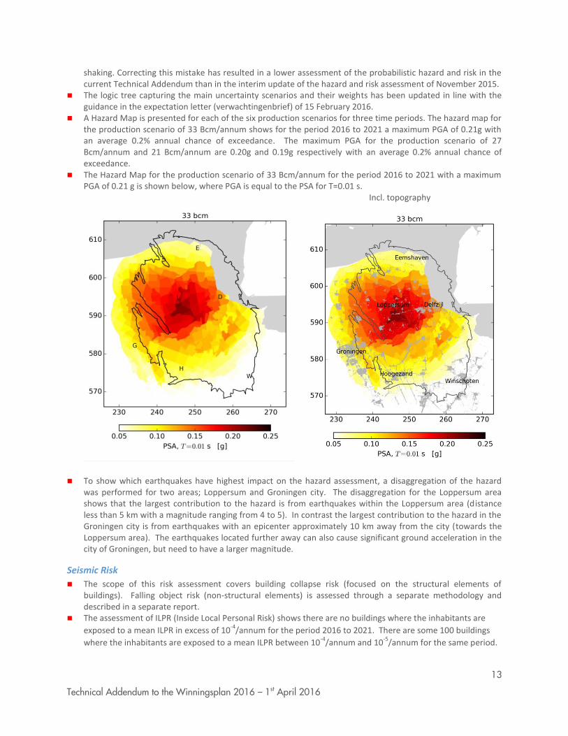
All available data (pressure, production, PNL etc.) for those fields were included in the history matching process in the same way as those from the main Groningen field. In addition to updated historical data, new well data have been included. This includes newly drilled Groningen wells Borgesweer-5 and Zeerijp-2 and 3 and data from the abandoned non-Groningen well Sauwerd-1. The 2012 and 2015 models are compared in Figure 2.1, with initial gas distribution shown in blue.
21
Technical Addendum to the Winningsplan 2016 – 1st April 2016
Figure 2.1 GFR2012 (left) and GFR2015 (right) grid boundary comparison.
The main updates to the dynamic model are listed below:
The same dynamic modelling package is used for GFR2015 (Shell software; MoReS and Reduce++),
but all input has been revised – tuning parameters have been removed, scripts have been cleaned-up
and standard functionality used where possible.
New subsidence proxy calculation and match quality indicator (normalised RMSE for subsidence) in
MoReS
Modified assignment of analytical aquifers, combined with different approach to tuning their
parameters for history matching and uncertainty evaluation
Revised set of saturation functions including Brooks-Corey based capillary pressure correlation and
improved relative permeability model
Revised fluid (PVT) properties including implicit modelling of condensed water in the gas phase based
on Wehe-McKetta
More constrained history matching workflow, with 3 matching parameters instead of 2.
One of the main objectives of the new dynamic model update is to achieve a history match to measured subsidence data, in addition to the more conventional match on reservoir pressure and gas-water contact. The approach chosen is to build an approximate, fast and integrated subsidence proxy in Mores. The proxy guides the history matching and is used in the uncertainty management workflow. It is important to note that the history match of subsidence is mostly used to improve our prediction of reservoir pressure, especially where we don’t have measured well data like for example in the aquifer. The final prediction of subsidence will be done using a separate full-physics geomechanical model, taking predicted reservoir pressure as input. Figure 2.2 and Figure 2.3 below show the theory and schematic representation of this proxy.

22
Technical Addendum to the Winningsplan 2016 – 1st April 2016
Figure 2.2 Subsidence modelling schematic
Figure 2.3 Subsidence proxy implementation and workflow
2.3 Dynamic model update since November 2015 HRA In November 2015 NAM prepared an intermediate report to the Hazard and Risk Assessment where an earlier version of the model described here was used. That model is referred to as “Dynamic model version 2 (GFR2015_v2)”. Since then several changes have been made to the model. The updated model that is used for this Winningsplan submission is referred to as GFR2015_v2.5.
The underlying static model of both versions is the same and was described in Section 2.2. Also, the reservoir behaviour, drive mechanisms and most of the match parameters did not change. However, there are some tuning parameters that have been changed to improve the quality of the simulation model. The differences are discussed in the History Matching section. Below are the main differences between the two models in descending importance.
Reservoir (3D)
Surface map, z=0 (2D)(0,0,0)
y
z
x
Lzn
Lxn
lxn
lzn
Footer: Title may be placed here or disclaimer if required. May sit up to two lines in depth.
Model subsidence proxy
Subsidence data
Model update & matching

23
Technical Addendum to the Winningsplan 2016 – 1st April 2016
1. All permeability multipliers in the aquifers have been removed while maintaining an equal or better
history match. The higher pressure in the aquifer, needed to achieve a match to subsidence, is now
obtained by changing the sealing behaviour of faults rather than from reducing aquifer permeability.
There are now only three global permeability multipliers left in the model:
a. Ten Boer reduction
b. Ameland shale reduction
c. Heterolithics reduction
2. Improved match on non-Groningen wells such as Bedum, Sauweerd, Kiel-Windeweer, Annerveen-
Veendam etc. The match was improved by the following steps:
a. Closer cross discipline collaboration with the Land Asset staff to better understand particular
reservoir features including fault sealing.
b. Volume corrections of Land fields according to the latest ARPR data.
3. Updated subsidence dataset resulting in improved match across the field
4. Update to relative permeability model where residual gas saturation is a function of porosity
5. Changes to PVT model, resulting in improved match of condensed water production
6. Well interface properties (kdh, Re) are derived from the fine scale model using the flow based upscaling.
Also, a vertical permeability reduction factor was introduced in the dynamic model in consultation with
geologists.
2.4 Dynamic Compartments and Initialization The initial pressure in Groningen at the free water level (FWL) is assumed to follow the hydrostatic gradient. However, there is not a single contact level across the Groningen field even though all parts are in pressure communication. No significant changes to FWLs are introduced for this work compared to the GFR2012 dynamic models. The set of FWLs are determined from a combination of open-hole logs, RFT and SPTG measurements, and define the set of dynamic compartments. The exact delineation between compartments follows faults and structures and also remains largely unchanged. There is also a temperature variation across the field, with a variation from about 80 to 120° C, resulting in different gas properties. All these variations are taken into account during the hydrostatic initialization. For the additional land fields, contact information is obtained from the corporate database, with a single level for each field. Figure 2.44 shows the dynamic compartments with corresponding FWLs (left). The area of the model that has an initial GWC within the Slochteren formation is also shown (right). In the south the contact is located in the Carboniferous.
Figure 2.4 Groningen field compartments with different FWL in TVNAP (left). GWC in the model (right)
24
Technical Addendum to the Winningsplan 2016 – 1st April 2016
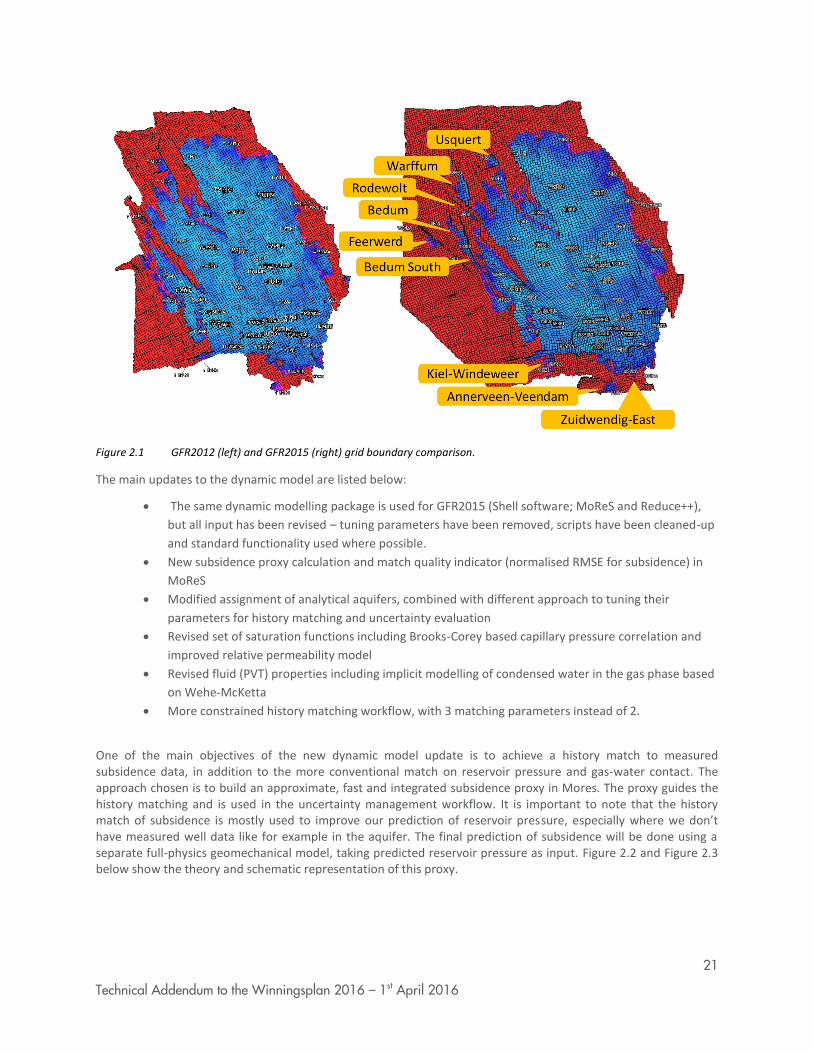
Geological fault throws and sand face juxtaposition as well as the origin of the faults define the sealing capability of the faults, and consequently the flowing paths for the fluid. In Figure 2.5 two east-west cross sections are shown. The major faults separating the north-east (where the ZND cluster is located) from Zeerijp and the north-west (where the ZRP wells are found) are clearly visible (top). Similarly there are faults separating the north-west from the east (bottom).
Figure 2.5 Faults with significant throw control the dynamic behaviour of the field
While the main input to the history matching process is agreement to pressure, PNL and subsidence data, the model was also checked to ensure that the hydrostatic initialization remains stable in time. It is clear that all parts of the Groningen field are in pressure communication, although many of the faults act as baffles between the different initialization regions. To validate the stability of the initialization, the model has been simulated for 1000 years without any production. In Figure 2.6 the gas water contact (GWC) at various locations is depicted as a function of time.
BDM PAU
ODP ZNDZRP

25
Technical Addendum to the Winningsplan 2016 – 1st April 2016
Figure 2.6 Stability of GWC in selected regions over a simulation period of 1000 years
From Figure 2.6 it is clear that the GWC in the different regions do show sufficient stability for the purposes of dynamic modelling. Only in the northern part of the Harkstede block (Eemskanaal-13 well location) is there some movement of the contact due to equilibration with the Eemskanaal region. However, the process is quite slow and the contact remains stable within the timeframe where the field is under production.
2.5 History matching workflow GFR 2015 dynamic model is constrained by the following historical data:
Production and injection data as controlling parameters
Pressure data including SP(T)Gs, CITHPs, BUs and RFTs
PNL data (water rise)
Subsidence data
Fluid composition data is not directly used in the history-matching process, however the changing gas composition in certain wells was evaluated during the analysis of the reservoir behaviour.
The subsidence data was matched using the subsidence proxy calculation and match quality indicator (normalised RMSE for subsidence) using MoReS (Shell’s in-house dynamic simulator). An example of the proxy results is shown in Figure 2.122.
An initial “reference” model was manually tuned based on the general understanding of the reservoir behaviour and results from the previous Groningen field reviews. A preliminary understanding of the behaviour of the surrounding Land asset fields had to be created, ensuring that no pressure communication exists with main Groningen field. Then the reference model was used as an input to the Assisted History Matching (AHM) workflow. This workflow serves to investigate many realisations with different variables and hence gives an insight into the various history matching possibilities. The following matching parameters were used to tune the model:
24 global and local Gross Block Volume (GBV) and permeability multipliers
38 fault grouping sealing factors
Other tuning parameters like aquifer properties, well inflow properties (skin) etc.
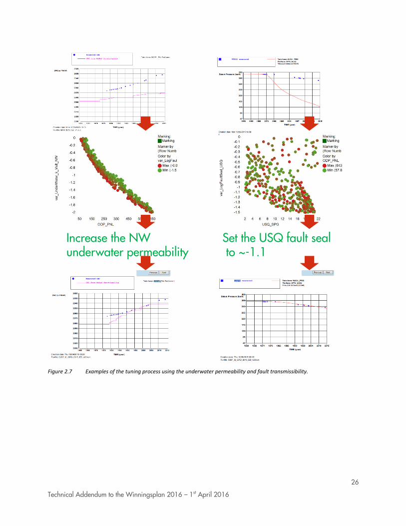
Figure 2.7 shows two examples of the assisted tuning of permeability and fault transmissibility to better match PNL and historical pressure data. Local match quality indicators suggest tuning parameters, e.g. an exact value of fault transmissibility in order to minimise the mismatch in certain areas.
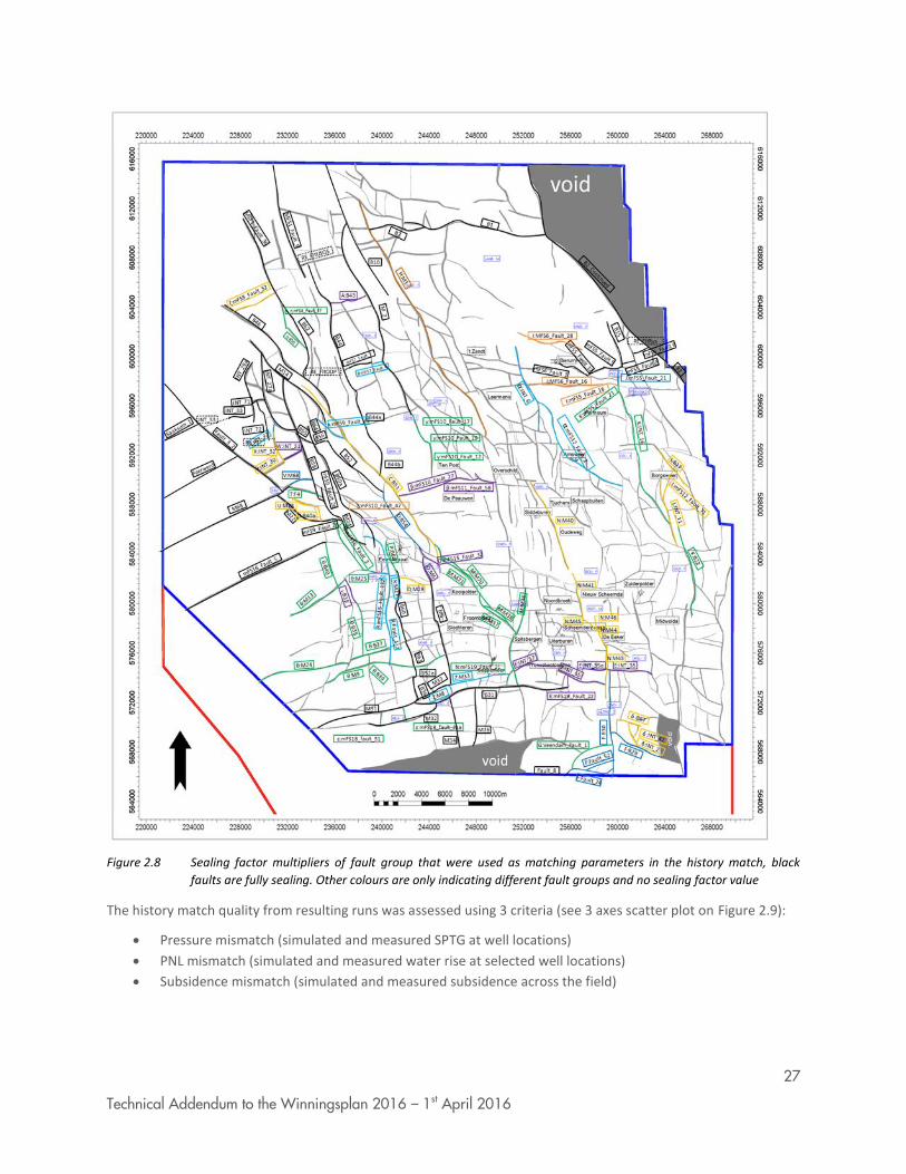
A map with the fault groupings are shown in Figure 2.8. It demonstrates that the transmissibility of the vast majority of fault groups had to be calibrated in order to match the dynamic behaviour of the field. Only a relative small set (marked in black) of faults were set to fully sealing. This increases the confidence that the impact of faults on reservoir behaviour is well understood.
26
Technical Addendum to the Winningsplan 2016 – 1st April 2016
Figure 2.7 Examples of the tuning process using the underwater permeability and fault transmissibility.
Increase the NW underwater permeability
Set the USQ fault sealto ~-1.1
27
Technical Addendum to the Winningsplan 2016 – 1st April 2016
Figure 2.8 Sealing factor multipliers of fault group that were used as matching parameters in the history match, black
faults are fully sealing. Other colours are only indicating different fault groups and no sealing factor value
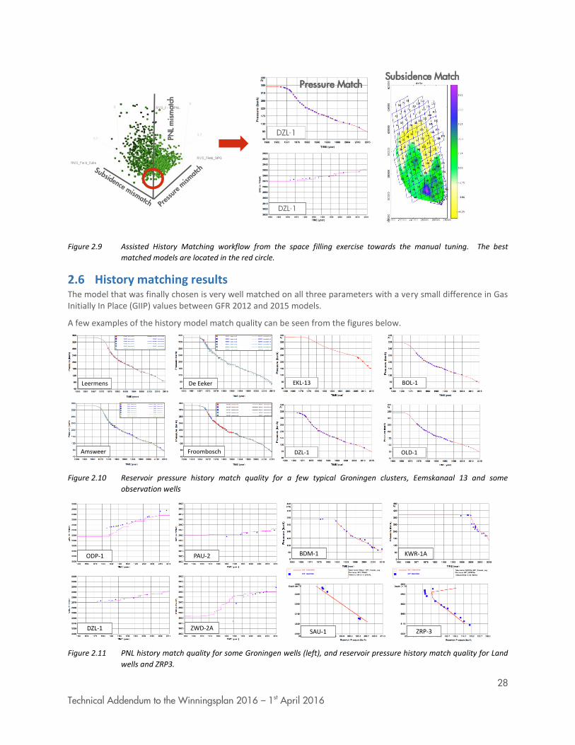
The history match quality from resulting runs was assessed using 3 criteria (see 3 axes scatter plot on Figure 2.9):
Pressure mismatch (simulated and measured SPTG at well locations)
PNL mismatch (simulated and measured water rise at selected well locations)
Subsidence mismatch (simulated and measured subsidence across the field)
28
Technical Addendum to the Winningsplan 2016 – 1st April 2016
Figure 2.9 Assisted History Matching workflow from the space filling exercise towards the manual tuning. The best
matched models are located in the red circle.
2.6 History matching results The model that was finally chosen is very well matched on all three parameters with a very small difference in Gas Initially In Place (GIIP) values between GFR 2012 and 2015 models.
A few examples of the history model match quality can be seen from the figures below.
Figure 2.10 Reservoir pressure history match quality for a few typical Groningen clusters, Eemskanaal 13 and some
observation wells
Figure 2.11 PNL history match quality for some Groningen wells (left), and reservoir pressure history match quality for Land
wells and ZRP3.
PNL
mis
mat
ch
Pressure MatchSubsidence Match
Leermens
Amsweer
De Eeker
Froombosch
EKL-13 BOL-1
DZL-1 OLD-1
PAU-2ODP-1
DZL-1 ZWD-2A
BDM-1 KWR-1A
SAU-1 ZRP-3

29
Technical Addendum to the Winningsplan 2016 – 1st April 2016
Figure 2.12 History match quality on subsidence using the proxy in Mores (scale is in cm).
2.7 Uncertainty analysis workflow and results The calibrated dynamic model provides reservoir pressures for the selected production scenarios and possibly includes the uncertainty range in reservoir pressures associated with subsurface uncertainty.
The history matched model and the resulting variable space will be used in the determination of ultimate recovery for a simplified production scenario. It is very important to use UR instead of GIIP for the uncertainty analysis, because the late field life uncertainty parameters are screened out in the selection based on GIIP, e.g. aquifers or relative permeability parameters. For reserve purposes the uncertainty in field UR at the end of economic field production life is important. For infill projects the uncertainty in project UR or project value is looked for and for hazard and risk assessment of earthquakes the uncertainty in maximum subsidence may be the parameter. This would imply that a different set of P10/P50/P90 models is used depending on the objectives.
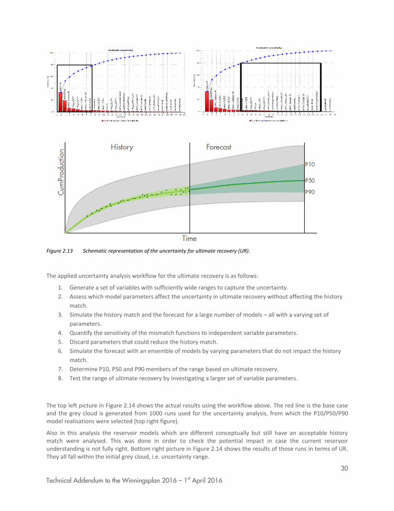
The goal is to have a set of models with a sufficient history match quality that captures the potential spread in the forecast and this is schematically shown in Figure 2.13. The top 2 graphs represent the screening criteria of the variables:
1. Left side box – less uncertain variables, because the history match quality is very sensitive to the change
of those variables
2. Right side box – variables that are not so sensitive for the history match, but might be important in late
life
Simulated Measured Difference
30
Technical Addendum to the Winningsplan 2016 – 1st April 2016
Figure 2.13 Schematic representation of the uncertainty for ultimate recovery (UR).
The applied uncertainty analysis workflow for the ultimate recovery is as follows:
1. Generate a set of variables with sufficiently wide ranges to capture the uncertainty.
2. Assess which model parameters affect the uncertainty in ultimate recovery without affecting the history
match.
3. Simulate the history match and the forecast for a large number of models – all with a varying set of
parameters.
4. Quantify the sensitivity of the mismatch functions to independent variable parameters.
5. Discard parameters that could reduce the history match.
6. Simulate the forecast with an ensemble of models by varying parameters that do not impact the history
match.
7. Determine P10, P50 and P90 members of the range based on ultimate recovery.
8. Test the range of ultimate recovery by investigating a larger set of variable parameters.
The top left picture in Figure 2.14 shows the actual results using the workflow above. The red line is the base case and the grey cloud is generated from 1000 runs used for the uncertainty analysis, from which the P10/P50/P90 model realisations were selected (top right figure).
Also in this analysis the reservoir models which are different conceptually but still have an acceptable history match were analysed. This was done in order to check the potential impact in case the current reservoir understanding is not fully right. Bottom right picture in Figure 2.14 shows the results of those runs in terms of UR. They all fall within the initial grey cloud, i.e. uncertainty range.

31
Technical Addendum to the Winningsplan 2016 – 1st April 2016
The bottom left picture shows the correlation between the UR and Subsidence values generated from the 1000 models. It is clearly seen that no correlation exists between to parameters and 3 separate low/mid/high models should be used for UR and subsidence calculations.
Figure 2.14 History match quality on subsidence using the proxy in Mores (scale is in cm).
32
Technical Addendum to the Winningsplan 2016 – 1st April 2016
3 The Groningen System 3.1 Gas Production System The Groningen System consists of the Groningen Field and the three Underground Gas Storages (UGS), the hi-cal UGS in Grijpskerk, the lo-cal UGS in Norg and the lo-cal PGI Alkmaar operated by TAQA.
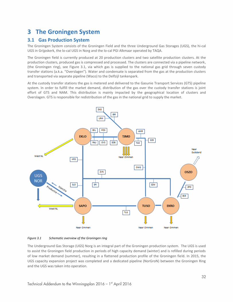
The Groningen field is currently produced at 20 production clusters and two satellite production clusters. At the production clusters, produced gas is compressed and processed. The clusters are connected via a pipeline network, (the Groningen ring), see Figure 3.1, via which gas is supplied to the national gas grid through seven custody transfer stations (a.k.a. “Overslagen”). Water and condensate is separated from the gas at the production clusters and transported via separate pipeline (Waco) to the Delfzijl tankenpark.
At the custody transfer stations the gas is metered and delivered to the Gasunie Transport Services (GTS) pipeline system. In order to fulfill the market demand, distribution of the gas over the custody transfer stations is joint effort of GTS and NAM. This distribution is mainly impacted by the geographical location of clusters and Overslagen. GTS is responsible for redistribution of the gas in the national grid to supply the market.
Figure 3.1 Schematic overview of the Groningen ring
The Underground Gas Storage (UGS) Norg is an integral part of the Groningen production system. The UGS is used
to assist the Groningen field production in periods of high capacity demand (winter) and is refilled during periods
of low market demand (summer), resulting in a flattened production profile of the Groningen field. In 2015, the
UGS capacity expansion project was completed and a dedicated pipeline (NorGroN) between the Groningen Ring
and the UGS was taken into operation.
33
Technical Addendum to the Winningsplan 2016 – 1st April 2016
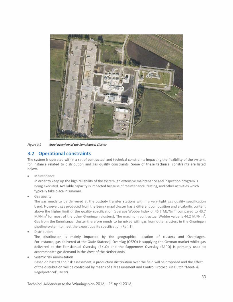
Figure 3.2 Areal overview of the Eemskanaal Cluster
3.2 Operational constraints The system is operated within a set of contractual and technical constraints impacting the flexibility of the system, for instance related to distribution and gas quality constraints. Some of these technical constraints are listed below.
Maintenance
In order to keep up the high reliability of the system, an extensive maintenance and inspection program is
being executed. Available capacity is impacted because of maintenance, testing, and other activities which
typically take place in summer.
Gas quality
The gas needs to be delivered at the custody transfer stations within a very tight gas quality specification
band. However, gas produced from the Eemskanaal cluster has a different composition and a calorific content
above the higher limit of the quality specification (average Wobbe Index of 45.7 MJ/Nm3, compared to 43.7
MJ/Nm3 for most of the other Groningen clusters). The maximum contractual Wobbe value is 44.2 MJ/Nm
3.
Gas from the Eemskanaal cluster therefore needs to be mixed with gas from other clusters in the Groningen
pipeline system to meet the export quality specification (Ref. 1).
Distribution
The distribution is mainly impacted by the geographical location of clusters and Overslagen.
For instance, gas delivered at the Oude Statenzijl Overslag (OSZO) is supplying the German market whilst gas
delivered at the Eemskanaal Overslag (EKLO) and the Sappemeer Overslag (SAPO) is primarily used to
accommodate gas demand in the West of the Netherlands.
Seismic risk minimization
Based on hazard and risk assessment, a production distribution over the field will be proposed and the effect
of the distribution will be controlled by means of a Measurement and Control Protocol (in Dutch “Meet- &
Regelprotocol”; MRP).
34
Technical Addendum to the Winningsplan 2016 – 1st April 2016
Other factors
Other constraints impacting available capacity and/or system flexibility include ambient temperature, GTS
system pressure and local demand, unforeseen unavailability of clusters
3.2.1 UGS injection requirements The UGS expansion project has led to a working volume increase from 3 to 7 bcm. In order to be able to inject the full 7bcm, the injection compressors require a high level of availability and a minimum level of suction pressure which can only be supplied via the NorGroN pipeline combined with a specific pressure segregation of the Groningen Ring. This segregation impacts the operational flexibility in terms of distribution.
3.2.2 Minimum flow Minimum flow rates at the overslagen
Every single custody transfer system (overslagen, OV) requires a minimum of 1 mln Nm3/day to keep it in
operation. Also the combination of OV’s with flows to the West (SAP and EKL), South (TJM, EKR, TUS and SAP) and East (OSZ) requires a minimum flow of 3 mln Nm
3/day per direction (East, South, East) for direct delivery to GTS.
Oudestatenzijl (OSZ) has a different character compared to other custody transfer stations, because of operational limitations in the GTS system, pressure and flow is required from the Groningen Ring (so called open pipe).
Minimum flow rates at clusters
Quick response to increase demand can only be facilitated from clusters in operation or in standby mode. The standby mode requires a minimum flow which is related to ambient temperature.
Minimum flow at high ambient temperatures: 1 mln m3/d (above 0 degrees Celsius)
Minimum flow at low ambient temperatures: 3 mln m3/d (between -10 and 0 degrees Celsius)
If the ambient temperature is below -10 degrees Celsius, the required minimum flow is higher.
35
Technical Addendum to the Winningsplan 2016 – 1st April 2016
4 Reduction of seismic risk through production management 4.1 Introduction This chapter investigates the possibility of reducing seismic risk by optimizing the offtake distribution over the field at a given annual total offtake level. This comes down to reducing the offtake from higher risk areas balanced by increasing offtake in lower-risk areas based on the current knowledge of the field. The approach and the optimization can be updated when new data become available and regularly reviewed as part of the measurement and control protocol. The seismic response to the changes in the distribution of the field offtake and resulting impact on risk can then guide future cycles in this optimization process. Gas production leads to pressure depletion, which in turn leads to reservoir compaction. Compaction and the consequential fault slip is the driving force for seismic activity. Therefore, pressure depletion is a preamble for seismic activity. Different production scenarios result in different pressure depletion trends in the field, and hence potentially in a different distribution of seismic risk. The operational constraints discussed in the previous chapter have to be incorporated in the design of production allocation scenarios. The optimisation approach and choices made therein is subject of a review process and are to be evaluated amongst others through steps described in the Measurement and Control Protocol. The effects of gas production from the Groningen field are monitored using different parameters such as pressure, subsidence, ground motion and seismic activity rate. A Measurement and Control Protocol has been written up in which a number of measured signal parameters have been identified which have an impact on the Hazard and Risk level. Based on these signal parameters values and observed trends, production distribution can or may be confirmed or redistributed over the field, taking into account the overall volume limitations. Regular reporting of measurements, trends, redistribution of production, and when required recalibration of the HRA models is part of the protocol. The “Hazard and Risk Assessment – interim update November 2015” (Nov 2015 HRA) is used as a starting point for the optimization as described in this chapter. In subsequent chapters of this technical addendum, hazard and risk assessments will be presented for both production allocation scenarios. This enables evaluation of the impact of production management on seismic risk. Further investigations to achieve a more robust and mathematically more rigorous optimization in the future are described in the “Study and Data Acquisition Plan”.
4.2 Hazard and Risk Assessment – Interim update November 2015
4.2.1 January 2015 regions The first initiative to influence, or rather reduce, seismic activity in the near term was taken by SodM, who advised to subdivide the Groningen field into four production regions (Figure 4.1) and assign production caps for each region. This advice was adopted and set as permit conditions by the Minister of Economic Affairs and implemented by NAM as follows:
LOPPZ1 clusters: 3.0 N.Bcm per year
2
Eemskanaal cluster: 2.0 N.Bcm per year
South-West clusters: 9.9 N.Bcm per year
East clusters: 24.5 N.Bcm per year
leading to a field total of 39.4 N.Bcm.
1 LOPPZ = Leermens, Overschild, De Paauwen, Ten Post and ‘t Zandt 2 N.Bcm refers to a volume of a billion normal cubic meters. Normal means the volume is measured at a standard temperature (0 degreeC) and pressure (1 bar).

36
Technical Addendum to the Winningsplan 2016 – 1st April 2016
These caps have been revised in 2015. The Council of State (Raad van State) ruled that the LOPPZ clusters could
only be produced to ensure security of supply, effectively reducing production to the volume required to keep
these clusters on warm stand-by (see Chapter 3). Later in that year, the total field production cap was further
reduced to 33 Bcm and 27 Bcm.
Figure 4.1 Production regions as per January 2015
4.2.2 Pressure response driven by January 2015 regions The production profiles as used in the Nov 2015 HRA were driven by the regions as they were enforced by the (revised) decision on the Winningsplan 2013. Figure 4.2 presents the forecasted reservoir pressure distribution for 2021 assuming a continuous cap on LOPPZ, showing a strong North-South trend in the associated pressure depletion. A consequence of the almost complete close-in of the five LOPPZ clusters is that the northern-most area of the field is less drained and only reaches a reservoir pressure of around 80 bar in 2021. The reservoir pressure in the south-eastern area of the field is expected to decline to some 50 bar, resulting in a pressure difference between these areas of 25 – 30 bar by 2021. The small depleted (blue) area to the west of the Groningen field is the Bedum field.
37
Technical Addendum to the Winningsplan 2016 – 1st April 2016
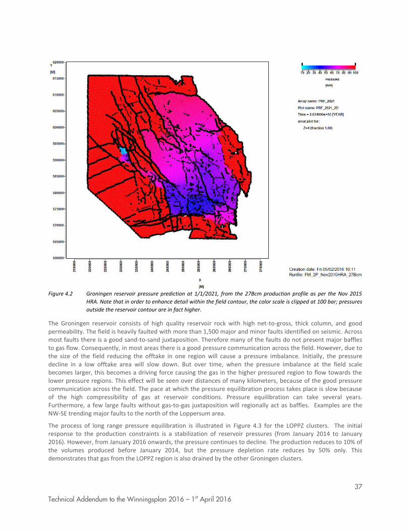
Figure 4.2 Groningen reservoir pressure prediction at 1/1/2021, from the 27Bcm production profile as per the Nov 2015
HRA. Note that in order to enhance detail within the field contour, the color scale is clipped at 100 bar; pressures
outside the reservoir contour are in fact higher.
The Groningen reservoir consists of high quality reservoir rock with high net-to-gross, thick column, and good permeability. The field is heavily faulted with more than 1,500 major and minor faults identified on seismic. Across most faults there is a good sand-to-sand juxtaposition. Therefore many of the faults do not present major baffles to gas flow. Consequently, in most areas there is a good pressure communication across the field. However, due to the size of the field reducing the offtake in one region will cause a pressure imbalance. Initially, the pressure decline in a low offtake area will slow down. But over time, when the pressure imbalance at the field scale becomes larger, this becomes a driving force causing the gas in the higher pressured region to flow towards the lower pressure regions. This effect will be seen over distances of many kilometers, because of the good pressure communication across the field. The pace at which the pressure equilibration process takes place is slow because of the high compressibility of gas at reservoir conditions. Pressure equilibration can take several years. Furthermore, a few large faults without gas-to-gas juxtaposition will regionally act as baffles. Examples are the NW-SE trending major faults to the north of the Loppersum area.
The process of long range pressure equilibration is illustrated in Figure 4.3 for the LOPPZ clusters. The initial response to the production constraints is a stabilization of reservoir pressures (from January 2014 to January 2016). However, from January 2016 onwards, the pressure continues to decline. The production reduces to 10% of the volumes produced before January 2014, but the pressure depletion rate reduces by 50% only. This demonstrates that gas from the LOPPZ region is also drained by the other Groningen clusters.
38
Technical Addendum to the Winningsplan 2016 – 1st April 2016
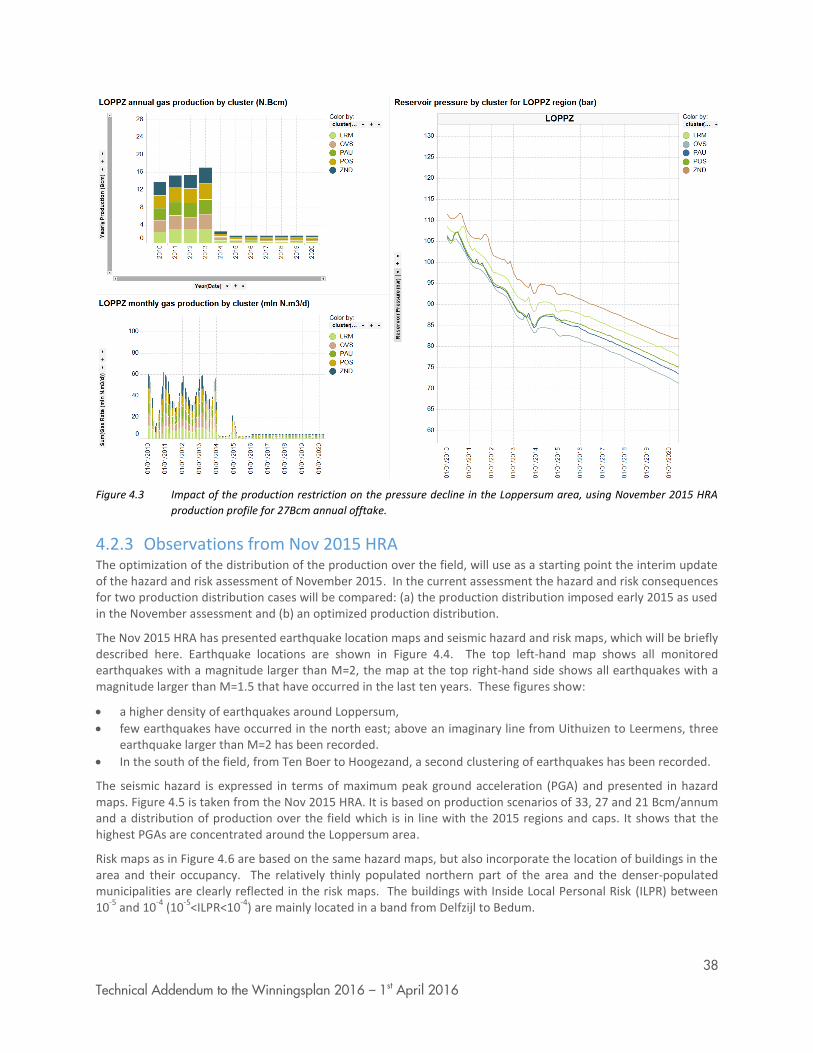
Figure 4.3 Impact of the production restriction on the pressure decline in the Loppersum area, using November 2015 HRA
production profile for 27Bcm annual offtake.
4.2.3 Observations from Nov 2015 HRA The optimization of the distribution of the production over the field, will use as a starting point the interim update of the hazard and risk assessment of November 2015. In the current assessment the hazard and risk consequences for two production distribution cases will be compared: (a) the production distribution imposed early 2015 as used in the November assessment and (b) an optimized production distribution.
The Nov 2015 HRA has presented earthquake location maps and seismic hazard and risk maps, which will be briefly described here. Earthquake locations are shown in Figure 4.4. The top left-hand map shows all monitored earthquakes with a magnitude larger than M=2, the map at the top right-hand side shows all earthquakes with a magnitude larger than M=1.5 that have occurred in the last ten years. These figures show:
a higher density of earthquakes around Loppersum,
few earthquakes have occurred in the north east; above an imaginary line from Uithuizen to Leermens, three earthquake larger than M=2 has been recorded.
In the south of the field, from Ten Boer to Hoogezand, a second clustering of earthquakes has been recorded.
The seismic hazard is expressed in terms of maximum peak ground acceleration (PGA) and presented in hazard maps. Figure 4.5 is taken from the Nov 2015 HRA. It is based on production scenarios of 33, 27 and 21 Bcm/annum and a distribution of production over the field which is in line with the 2015 regions and caps. It shows that the highest PGAs are concentrated around the Loppersum area.
Risk maps as in Figure 4.6 are based on the same hazard maps, but also incorporate the location of buildings in the area and their occupancy. The relatively thinly populated northern part of the area and the denser-populated municipalities are clearly reflected in the risk maps. The buildings with Inside Local Personal Risk (ILPR) between 10
-5 and 10
-4 (10
-5<ILPR<10
-4) are mainly located in a band from Delfzijl to Bedum.

39
Technical Addendum to the Winningsplan 2016 – 1st April 2016
Period: 1986 – 2016, Earthquakes M>=2.0 Period: 2006 – 2016, Earthquakes M>=1.5
Period: Up to January 2016
Figure 4.4 Historical earthquakes in Groningen. Top row on the left all earthquakes with a magnitude larger than M = 2 are
shown, while at the right all earthquakes with a magnitude larger than M=1.5 for the last ten years are shown.
Bottom row gives all historic earthquakes with a magnitude larger than or equal to M=3.0

40
Technical Addendum to the Winningsplan 2016 – 1st April 2016
Figure 4.5 Mean PGA hazard sensitivity to production rates. Period: 2016/1 – 2021/1 (from Figure 4.14 of Nov 2015 HRA)
10-4<ILPR<10-3
(buildings 0)
10-5<ILPR<10-4
(buildings c. 4000)
Figure 4.6 Mean inside local personal risk, ILPR for every individual building within two equal risk bands (from 10-5
to
10-4
/year, and from 10-4
to 10-3
/year) for the 5-year assessment period 2016 to 2021 under the 33 Bcm
production scenario without structural upgrading. (from Nov 2015 HRA)
Figures 4.5 and 4.6 have been taken from the Interim Update of the Hazard and Risk Assessment of November
2015, which served as the starting point for the optimisation of the production distribution over the field.

41
Technical Addendum to the Winningsplan 2016 – 1st April 2016
4.3 Optimisation of the production distribution
4.3.1 Considerations The January 2015 production regions were introduced to steer production distribution over the field. In order to influence seismic risk these regions should be defined in line with the gas flow behavior of the field. The following factors need to be taken into account:
Gas flow and pressure behavior in the reservoir
The distribution of clusters in the field
Operational constraints in the production and pipeline systems
Figure 4.7 combines all these elements. It gives a saturation map of the reservoir with a schematic of the production system, the net hydrocarbon column map for the field, and two streamline graphs. One graph shows the streamlines colored by arriving producer, indicating the direction of flow. The other graph is colored by drainage time, i.e. the time it takes for a gas particle to travel along a streamline from a position in the reservoir to a producer well. Streamlines seem to be preferentially oriented along a NW-SE trend. The same trend is also seen in the orientation of structural elements. This suggests that those elements are affecting gas flow through the reservoir. Hence, from a gas flow and reservoir pressure perspective it makes more sense to define production regions in line with these NW-SE trends.
The net hydrocarbon column map of Figure 4.7 can be considered as a proxy for the hypothetical compaction that
may occur in response to pressure depletion. It was mentioned earlier in this chapter that compaction is thought
to be the driving force for induced seismicity. Particularly those locations where differential compaction occurs on
either side of a fault may be prone to slippage. Therefore, the net hydrocarbon column map also provides insights
for the definition of production regions.

42
Technical Addendum to the Winningsplan 2016 – 1st April 2016
Figure 4.7 Drainage of the Groningen field

43
Technical Addendum to the Winningsplan 2016 – 1st April 2016
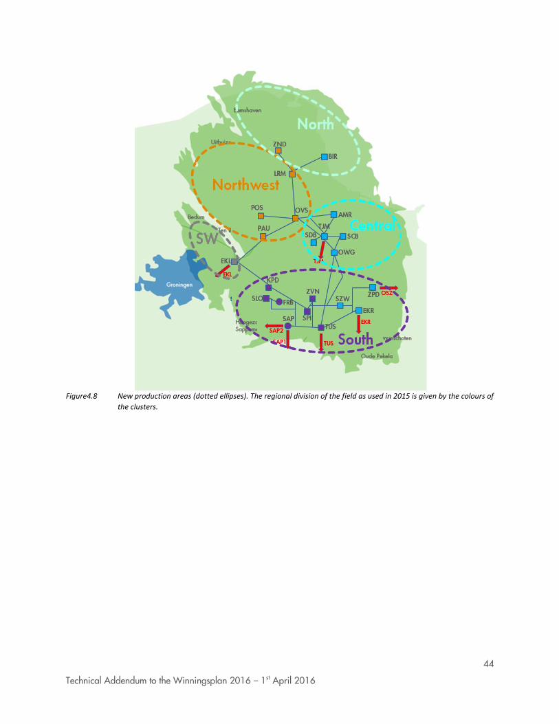
4.3.2 New areas Based on the above observations on reservoir pressure behavior, gas flow patterns and structural-geological aspects, an update is proposed for the subdivision of the Groningen field into production offtake areas. The newly defined areas are described below and are used to evaluate the effect of production optimization to reduce seismic risk.
4.3.2.1 North area
The most northern area of the Groningen field is characterized by a low fault density and a relatively high net gas column. The column height decreases gradually to the north-east. This region has seen very limited seismic activity to date.
4.3.2.2 Northwest area
This area is characterized by a high fault density and a high but laterally varying net gas column. The area was historically most prone to seismic activity and production from clusters located in this area has been set to a minimum level in January 2015. The area is bounded in the north by a fault.
4.3.2.3 Southwest area
This area has a slightly higher pressure than other areas of the Groningen field. This can be attributed to the presence of faults and a limited juxtaposition window with other areas of the field. Fault density is high in this region and the gas column is modest on average but laterally variable.
4.3.2.4 South area
The southern part of the Groningen field has the highest density of production clusters, and consequently has a uniform pressure distribution. Fault density is also high but the net column height is limited. Therefore, the expected total compaction is limited and seismic activity levels are expected to be limited as well.
4.3.2.5 Central area
The Central area is characterized by a high fault density and a high net gas column, but with limited lateral variability. Seismic activity has slightly increased over the past years. The area is geographically close to the industrialized zone around Delfzijl.
The new areas are schematically shown in figure 4.8 as ellipses. The subdivision in production regions as used in 2015 is indicated by the colours of the clusters.
These areas have been defined based on the latest insights into reservoir behavior and seismicity. They form the basic building blocks for the optimization of the distribution of production over the field. The Measurement and Control Protocol describes the procedures for monitoring both production in the regions and the seismic activity, which should allow for further optimization of production in the future.
44
Technical Addendum to the Winningsplan 2016 – 1st April 2016
Figure4.8 New production areas (dotted ellipses). The regional division of the field as used in 2015 is given by the colours of
the clusters.

45
Technical Addendum to the Winningsplan 2016 – 1st April 2016
5 Forecasting with the optimised production distribution 5.1 Introduction For the production forecasting, a combination of the subsurface model (MoRes) and surface network model (GenRem) has been used. The operational constraints as mentioned in section 3.2 and in addition, the forecast constraints as mentioned chapter 4.3 are taken into account.
5.2 Annual Demand profile SodM advice (of December 2015) and the expectation letter from the Minister (February 2016) request NAM to avoid rapid production fluctuations as this may reduce the seismic risk. The production strategy was therefore changed to targeting a constant average production volume level per month (with an operational margin).
This flat production target has been applied both on a field level, and on an areal level. Also, the latest long term shutdown planning (LTSP) including scheduled cluster shutdowns is taken into account.
5.3 Capacity The installed capacity in the Groningen field depends on the reservoir pressure and the operational status of the production clusters. Based on the applied maintenance strategy, the recorded performance and risk failure probability, an availability curve is established for the production facilities in the Groningen system. This availability curve indicates the expectation that a certain capacity is available for production.
In order to be able to produce the annual volume target at a flat annual demand profile, a minimum capacity is required and given the capacity per cluster consequently a certain number of production clusters. However, additional capacity is necessary because of the availabilities, the physical limitations of Groningen Ring and the GTS network, filling the UGS Norg and PGI Alkmaar, and any market restrictions.
5.4 Production logic In order to manage seismic risk, optimized offtake is such that production will be redistributed from areas of higher risk to areas of lower risk. The following logic was established to define the production policies:
Increase offtake in the North region. From streamlines, HC thickness map and pressure maps, it is clear that the North is under-utilized, and does not seem to interfere much with the Northwest region.
Reduce production from Southwest region.
Production from North-West utilization is limited.
5.5 Production Scenarios Three optimized production scenarios were simulated, which all honour the constraints as per section 3.2. Each production scenario assumes a constant offtake which has not been convoluted with market demand and does not cover for security of supply.
21 Bcm ; Regional productions are North 4 Bcm, Northwest 1.5 Bcm, Southwest 0.5 Bcm, South 10 Bcm, and
Central 5 Bcm. Within the South region highest priority is on ZPD/EKR/TUS/SZW/SAP, while the clusters closest
to the high risk North-West area (KPD/ZVN/SLO/SPI) will only produce gas when required.
In the Central region a low priority is given to SDB, since it is closest to North-West area (will only produce
when required).
27 Bcm; Regional productions are North 5.5 Bcm, Northwest 1.5 Bcm, Southwest 0.5 Bcm, South 14 Bcm, and
Central 5.5 Bcm.
33 Bcm; In order to maximise the production plateau the load factors per region were kept similar: the
production from the South region was increased with 1 Bcm to an annual total of 15 Bcm, and the Central
region to 10.5 Bcm.

46
Technical Addendum to the Winningsplan 2016 – 1st April 2016
All forecasts were started at 1/1/2016, at the end of the history match. Figure 5.1 gives their respective offtake profiles in annual volumes and monthly rates. Figure 5.2 gives the reservoir pressure depletion over the next 5 years (between 1/1/2016 and 1/1/2021) for the three scenarios. It can be seen that for all scenarios, pressure depletion is minimized in the Central-Western part of the field. However, for the high offtake scenario (33 Bcm), this effect becomes less pronounced, and especially the South is further depleted.
Figure 5.3 gives a direct comparison of the next 5 year’s depletion between the Nov 2015 HRA forecasts and the optimized new regional offtake pattern, for 21/27/33 Bcm annual offtake, together with their respective corresponding pressure differences. It is clear that with the new regions, the relatively benign North-Eastern area of the field is further utilized, at the benefit of the Southwestern (Eemskanaal) area, and extending the spared North-West area further South/East.
Note that the monthly production volumes are flat, taken into account maintenance, i.e. field loadfactor is the same every month.
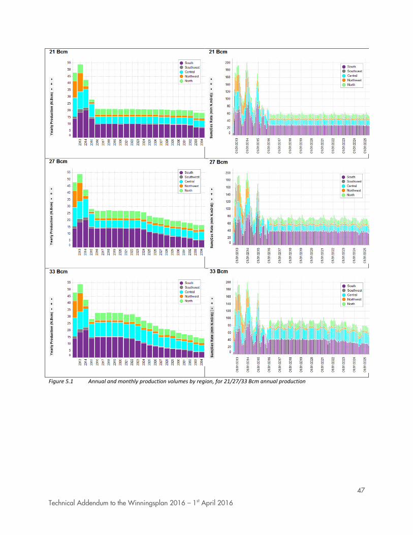
47
Technical Addendum to the Winningsplan 2016 – 1st April 2016
Figure 5.1 Annual and monthly production volumes by region, for 21/27/33 Bcm annual production
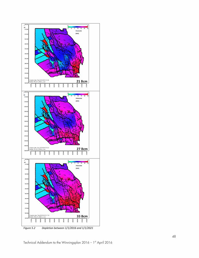
48
Technical Addendum to the Winningsplan 2016 – 1st April 2016
Figure 5.2 Depletion between 1/1/2016 and 1/1/2021
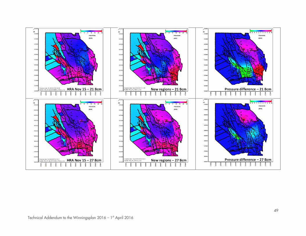
49
Technical Addendum to the Winningsplan 2016 – 1st April 2016

50
Technical Addendum to the Winningsplan 2016 – 1st April 2016
Figure 5.3 Pressure depletion between 1/1/2016 and 1/1/2021 for 21/27/33 Bcm annual offtake scenarios, comparing the “Nov 2015 HRA” production profile with the
optimised production distribution from the “New regions”
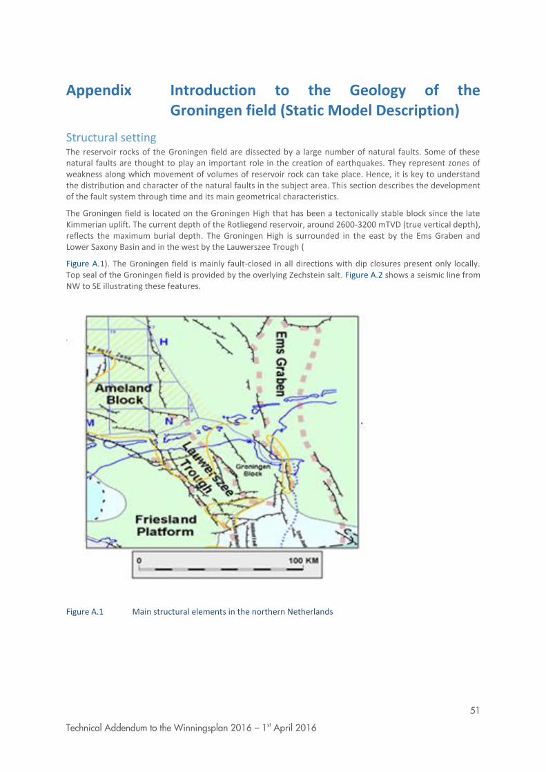
51
Technical Addendum to the Winningsplan 2016 – 1st April 2016
Appendix Introduction to the Geology of the Groningen field (Static Model Description)
Structural setting The reservoir rocks of the Groningen field are dissected by a large number of natural faults. Some of these natural faults are thought to play an important role in the creation of earthquakes. They represent zones of weakness along which movement of volumes of reservoir rock can take place. Hence, it is key to understand the distribution and character of the natural faults in the subject area. This section describes the development of the fault system through time and its main geometrical characteristics.
The Groningen field is located on the Groningen High that has been a tectonically stable block since the late Kimmerian uplift. The current depth of the Rotliegend reservoir, around 2600-3200 mTVD (true vertical depth), reflects the maximum burial depth. The Groningen High is surrounded in the east by the Ems Graben and Lower Saxony Basin and in the west by the Lauwerszee Trough (
Figure A.1). The Groningen field is mainly fault-closed in all directions with dip closures present only locally. Top seal of the Groningen field is provided by the overlying Zechstein salt. Figure A.2 shows a seismic line from NW to SE illustrating these features.
Figure A.1 Main structural elements in the northern Netherlands
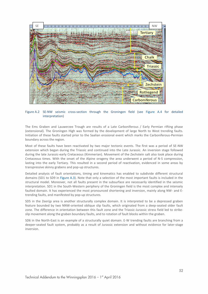
52
Technical Addendum to the Winningsplan 2016 – 1st April 2016
Figure A.2 SE-NW seismic cross-section through the Groningen field (see Figure A.4 for detailed interpretation)
The Ems Graben and Lauwerzee Trough are results of a Late Carboniferous / Early Permian rifting phase (extensional). The Groningen High was formed by the development of large North to West trending faults. Initiation of these faults started prior to the Saalian erosional event which marks the Carboniferous-Permian boundary across the region.
Most of these faults have been reactivated by two major tectonic events. The first was a period of SE-NW extension which began during the Triassic and continued into the Late Jurassic. An inversion stage followed during the late Jurassic-early Cretaceous (Kimmerian). Movement of the Zechstein salt also took place during Cretaceous times. With the onset of the Alpine orogeny the area underwent a period of N-S compression, lasting into the early Tertiary. This resulted in a second period of reactivation, evidenced in some areas by transpressive skinny grabens and pop-up structures.
Detailed analysis of fault orientations, timing and kinematics has enabled to subdivide different structural domains (SD1 to SD9 in Figure A.3). Note that only a selection of the most important faults is included in the structural model. Moreover, not all faults present in the subsurface are necessarily identified in the seismic interpretation. SD1 in the South-Western periphery of the Groningen field is the most complex and intensely faulted domain. It has experienced the most pronounced shortening and inversion, mainly along NW- and E-trending faults, and manifested by pop-up structures.
SD5 in the Zeerijp area is another structurally complex domain. It is interpreted to be a depressed graben feature bounded by two NNW-oriented oblique slip faults, which originated from a deep-seated older fault zone. The difference in orientation between this fault zone and the Triassic-Jurassic stress field led to strike-slip movement along the graben boundary faults, and to rotation of fault blocks within the graben.
SD6 in the North-East is an example of a structurally quiet domain. E-W trending faults are branching from a deeper-seated fault system, probably as a result of Jurassic extension and without evidence for later-stage inversion.
Tertiary
Chalk
Triassic
Zechstein
Rotliegend
Carboniferous
SE NW

53
Technical Addendum to the Winningsplan 2016 – 1st April 2016
Figure A.3 Structural domains in the Groningen field (total area ~ 40 x 40 km); faults shown are at Top_Rotliegend level
Stratigraphy and depositional setting A second important factor in the study of induced earthquakes, next to the structural model described above, is the distribution of rock properties in the reservoir. For example: the higher its porosity, the higher is the potential for the rock to compact as a result of gas production. The key role of compaction in generating seismicity is described in this technical addendum. Porosity is high in sandstone rock and low in claystones. The depositional processes that formed the sandstones are also important in the sense that rocks formed by wind action (aeolian sediments) generally have higher porosities than those formed by river currents (fluvial sediments). In the following, an overview is given of the important rock formations present in the subsurface of Groningen.
The gas-bearing interval in the Groningen field comprises both Upper Rotliegend Group (Permian) and Limburg Group (Carboniferous) sediments, separated by the Saalian Unconformity.
The Carboniferous sediments range in age from Westphalian-A to Westphalian-D. They represent lower to middle delta plain deposition under humid, subtropical conditions. The Carboniferous strata have been tilted and eroded during the Variscan orogeny (Figure A.4). This created a depositional relief that was gradually filled by the Rotliegend.
N
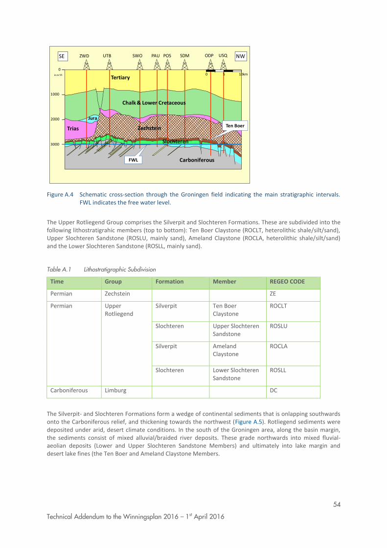
54
Technical Addendum to the Winningsplan 2016 – 1st April 2016
Figure A.4 Schematic cross-section through the Groningen field indicating the main stratigraphic intervals. FWL indicates the free water level.
The Upper Rotliegend Group comprises the Silverpit and Slochteren Formations. These are subdivided into the following lithostratigrahic members (top to bottom): Ten Boer Claystone (ROCLT, heterolithic shale/silt/sand), Upper Slochteren Sandstone (ROSLU, mainly sand), Ameland Claystone (ROCLA, heterolithic shale/silt/sand) and the Lower Slochteren Sandstone (ROSLL, mainly sand).
Table A.1 Lithostratigraphic Subdivision
Time Group Formation Member REGEO CODE
Permian Zechstein ZE
Permian Upper Rotliegend
Silverpit Ten Boer Claystone
ROCLT
Slochteren Upper Slochteren Sandstone
ROSLU
Silverpit Ameland Claystone
ROCLA
Slochteren Lower Slochteren Sandstone
ROSLL
Carboniferous Limburg DC
The Silverpit- and Slochteren Formations form a wedge of continental sediments that is onlapping southwards onto the Carboniferous relief, and thickening towards the northwest (Figure A.5). Rotliegend sediments were deposited under arid, desert climate conditions. In the south of the Groningen area, along the basin margin, the sediments consist of mixed alluvial/braided river deposits. These grade northwards into mixed fluvial-aeolian deposits (Lower and Upper Slochteren Sandstone Members) and ultimately into lake margin and desert lake fines (the Ten Boer and Ameland Claystone Members.
Tertiary
Chalk & Lower Cretaceous
ZechsteinTrias
Jura
ZWD UTB SWO PAU POS SDM ODP USQ
3000
2000
1000
0
NWSE
0 5 10kmin m SS
Carboniferous
Slochteren
Ten Boer
FWL
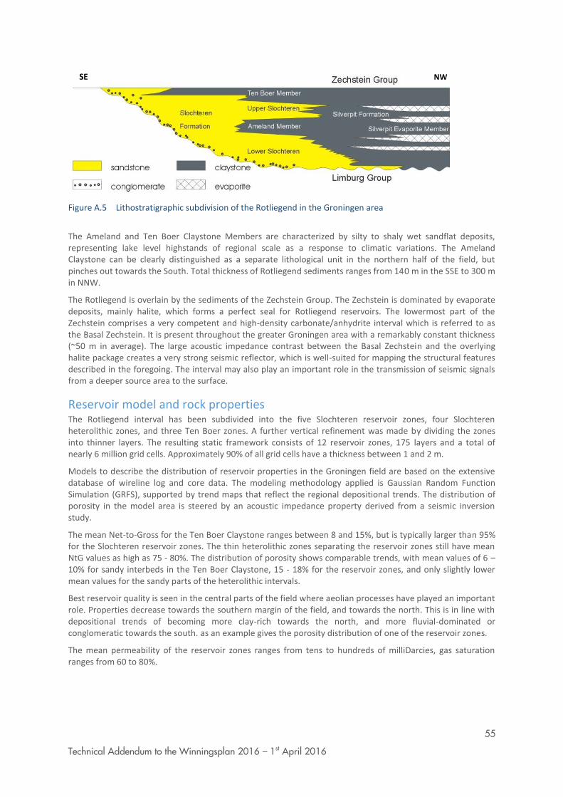
55
Technical Addendum to the Winningsplan 2016 – 1st April 2016
Figure A.5 Lithostratigraphic subdivision of the Rotliegend in the Groningen area
The Ameland and Ten Boer Claystone Members are characterized by silty to shaly wet sandflat deposits, representing lake level highstands of regional scale as a response to climatic variations. The Ameland Claystone can be clearly distinguished as a separate lithological unit in the northern half of the field, but pinches out towards the South. Total thickness of Rotliegend sediments ranges from 140 m in the SSE to 300 m in NNW.
The Rotliegend is overlain by the sediments of the Zechstein Group. The Zechstein is dominated by evaporate deposits, mainly halite, which forms a perfect seal for Rotliegend reservoirs. The lowermost part of the Zechstein comprises a very competent and high-density carbonate/anhydrite interval which is referred to as the Basal Zechstein. It is present throughout the greater Groningen area with a remarkably constant thickness (~50 m in average). The large acoustic impedance contrast between the Basal Zechstein and the overlying halite package creates a very strong seismic reflector, which is well-suited for mapping the structural features described in the foregoing. The interval may also play an important role in the transmission of seismic signals from a deeper source area to the surface.
Reservoir model and rock properties The Rotliegend interval has been subdivided into the five Slochteren reservoir zones, four Slochteren heterolithic zones, and three Ten Boer zones. A further vertical refinement was made by dividing the zones into thinner layers. The resulting static framework consists of 12 reservoir zones, 175 layers and a total of nearly 6 million grid cells. Approximately 90% of all grid cells have a thickness between 1 and 2 m.
Models to describe the distribution of reservoir properties in the Groningen field are based on the extensive database of wireline log and core data. The modeling methodology applied is Gaussian Random Function Simulation (GRFS), supported by trend maps that reflect the regional depositional trends. The distribution of porosity in the model area is steered by an acoustic impedance property derived from a seismic inversion study.
The mean Net-to-Gross for the Ten Boer Claystone ranges between 8 and 15%, but is typically larger than 95% for the Slochteren reservoir zones. The thin heterolithic zones separating the reservoir zones still have mean NtG values as high as 75 - 80%. The distribution of porosity shows comparable trends, with mean values of 6 – 10% for sandy interbeds in the Ten Boer Claystone, 15 - 18% for the reservoir zones, and only slightly lower mean values for the sandy parts of the heterolithic intervals.
Best reservoir quality is seen in the central parts of the field where aeolian processes have played an important role. Properties decrease towards the southern margin of the field, and towards the north. This is in line with depositional trends of becoming more clay-rich towards the north, and more fluvial-dominated or conglomeratic towards the south. as an example gives the porosity distribution of one of the reservoir zones.
The mean permeability of the reservoir zones ranges from tens to hundreds of milliDarcies, gas saturation ranges from 60 to 80%.
SE NW
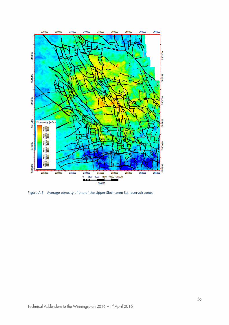
56
Technical Addendum to the Winningsplan 2016 – 1st April 2016
Figure A.6 Average porosity of one of the Upper Slochteren Sst reservoir zones

57
Technical Addendum to the Winningsplan 2016 – 1st April 2016
1
Technical Addendum to the Winningsplan 2016 – 1st April 2016
Technical Addendum to the Winningsplan Groningen 2016 Production, Subsidence, Induced Earthquakes and Seismic Hazard and Risk Assessment in the Groningen Field Part II Subsidence

2
Technical Addendum to the Winningsplan 2016 – 1st April 2016
The report “Technical Addendum to the Winningsplan Groningen 2016 - Production, Subsidence, Induced Earthquakes and Seismic Hazard and Risk Assessment in the Groningen Field” consists of five separate documents:
Document 1 Chapters 1 to 5; Summary and Production
Document 2 Chapter 6; Subsidence
Document 3 Chapter 7; Hazard
Document 4 Chapter 8; Risk
Document 5 Chapter 9; Damage and Appendices.
Each of these documents is also available as a *.pdf file of a size smaller than 10Mbyte, allowing sharing through e-mail.
© EP201603238413 Dit rapport is een weerslag van een voortdurend studie- en dataverzamelingsprogramma en bevat de stand der kennis van april 2016. Het copyright van dit rapport ligt bij de Nederlandse Aardolie Maatschappij B.V. Het copyright van de onderliggende studies berust bij de respectievelijke auteurs. Dit rapport of delen daaruit mogen alleen met een nadrukkelijke status-en bronvermelding worden overgenomen of gepubliceerd.
3
Technical Addendum to the Winningsplan 2016 – 1st April 2016
Table of Contents 6 Subsidence 4
6.1 Summary 4
6.2 Introduction 4
6.3 Geodetic and geomechanical data 5
6.3.1 Survey protocol 5
6.3.2 Surveying techniques 6
6.3.3 Survey design 6
6.3.4 Levelling and InSAR data used for the calibration 8
6.3.5 Data from uniaxial compaction experiments 9
6.4 The Groningen Geomechanical model 11
6.4.1 Time Decay Compaction model 12
6.4.2 Isotach formulation of the Rate Type Compaction model 13
6.4.3 Upscaling of input data 13
6.5 Calibration of the geomechanical model with geodetic data 15
6.5.1 RMS of all benchmarks using epoch combinations 15
6.5.2 Winningsplan 2013 spatial fit 16
6.5.3 Time Decay model 18
6.5.4 RTCiM model 19
6.5.5 Comparison 21
6.6 RTCiM and Time Decay response to changes in production 23
6.6.1 Selection of base case compaction model 23
6.7 Subsidence forecasts 24
6.8 Compaction forecast for the hazard calculation 28
4
Technical Addendum to the Winningsplan 2016 – 1st April 2016
6 Subsidence 6.1 Summary
This chapter presents in more technical detail the subsidence forecasts as presented in chapter 5 of the Groningen winningsplan. Land subsidence above the Groningen field is caused by compaction of the reservoir due to the gas production. In a first order approach the compaction in the reservoir can be calculated by multiplying the depleting thickness, the amount of depletion (or pressure drop) and the compressibility of the rock. Geodetic information above the field indicates however that the relationship between pressure drop and subsidence is not simply linear. The most logical explanation for this phenomenon is believed to be a more complex compaction behavior of the reservoir.
Therefore two compaction models are investigated for the Groningen subsidence calculations, both describing a non-linear relationship with pressure drop, i.e. the time decay (NAM, 2011) model and the rate type compaction isotach model (RTCiM, TNO2013). The time decay model, according to which compaction decays with time after a pressure perturbation, has been adopted in NAM for subsidence calculations since 2011.
Typically geodetic observations above the gas fields in The Netherlands show an increase of the subsidence rate after the first years of production. The first model used to match this observation was a bi-linear compaction model and this was used by NAM till 2011. However, when updating the Ameland winningsplan in 2010 it became apparent that the bi-linear model could not describe the ongoing subsidence observed above this field (NAM, 2011) with the decreasing depletion rate at the end of field life. An updated model to address this delayed subsidence both at the start and at the end of the production was adopted: the time decay compaction model. The time decay model has less free parameters than the bi-linear model while matching the full geodetic dataset above the field of Ameland using the compressibility (Cm)-porosity relation based on laboratory data.
A similar approach was followed for matching the subsidence above the Groningen field but in this case the aforementioned Cm-porosity trend line could not be used directly. A calibration factor of about 0.5 had to be applied to this trend line in order to obtain a good temporal and spatial match between modelled and measured subsidence. For the 2016 winningsplan, supported by this document, a spatially varying Cm value derived from a direct inversion of the geodetic data was used to further improve the match.
Besides the application of the time decay model, a second model was adopted from TNO (TNO, 2013), i.e. the RTCiM model. This model also provides a good match with the historical subsidence data but contains more degrees of freedom when compared to the time decay model.
Reservoir pressures from the Groningen MoReS model have been used as input for the compaction model. The distribution of reservoir porosity and thickness were taken from the static Petrel model and upscaled with the condition that the upscaled compaction be equal to the sum of the compaction of the individual layers.
A RMS method was used to check the “goodness-of-fit” between modelled and measured historic subsidence.
6.2 Introduction The Groningen field was discovered in 1959 and gas production started in 1963. Globally, the field belongs to the top-ten largest gas fields. Subsidence was recognised as a risk before production began and was monitored from the start through regular levelling surveys. Since 1993 also satellite based Interferometric Synthetic Aperture Radar (InSAR) measurements have been used for this purpose. In 2013 the first continuous GPS monitoring station in Groningen was installed in Ten Post.
The subsidence models were revised and refined through time as more data became available. Compaction models have to meet two basic criteria: they have to closely match the subsidence measurements and they should be based on plausible physical mechanisms. Section 6.3 will describe the availability of data, i.e., laboratory compaction data and geodetic data. Section 6.4 describes the geomechanics of the Groningen field including the compaction models and the importance of overburden behaviour. Subsequent sections (6.5 and 6.6) describe model calibration and the subsidence forecasts.
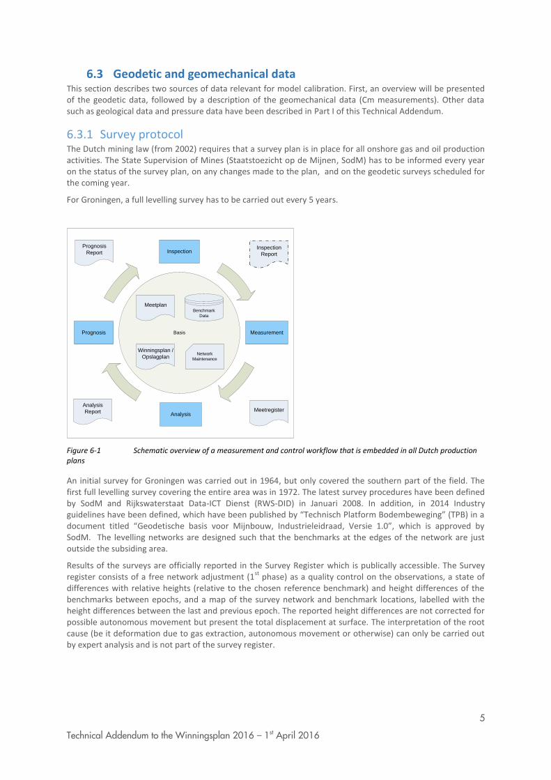
5
Technical Addendum to the Winningsplan 2016 – 1st April 2016
6.3 Geodetic and geomechanical data This section describes two sources of data relevant for model calibration. First, an overview will be presented of the geodetic data, followed by a description of the geomechanical data (Cm measurements). Other data such as geological data and pressure data have been described in Part I of this Technical Addendum.
6.3.1 Survey protocol The Dutch mining law (from 2002) requires that a survey plan is in place for all onshore gas and oil production activities. The State Supervision of Mines (Staatstoezicht op de Mijnen, SodM) has to be informed every year on the status of the survey plan, on any changes made to the plan, and on the geodetic surveys scheduled for the coming year.
For Groningen, a full levelling survey has to be carried out every 5 years.
Basis Measurement
MeetregisterAnalysis
Report
Inspection
Report
Prognosis
Analysis
Inspection
Meetplan
Winningsplan /
Opslagplan
Prognosis
Report
Network
Maintenance
Benchmark
Data
Figure 6-1 Schematic overview of a measurement and control workflow that is embedded in all Dutch production plans
An initial survey for Groningen was carried out in 1964, but only covered the southern part of the field. The first full levelling survey covering the entire area was in 1972. The latest survey procedures have been defined by SodM and Rijkswaterstaat Data-ICT Dienst (RWS-DID) in Januari 2008. In addition, in 2014 Industry guidelines have been defined, which have been published by “Technisch Platform Bodembeweging” (TPB) in a document titled “Geodetische basis voor Mijnbouw, Industrieleidraad, Versie 1.0”, which is approved by SodM. The levelling networks are designed such that the benchmarks at the edges of the network are just outside the subsiding area.
Results of the surveys are officially reported in the Survey Register which is publically accessible. The Survey register consists of a free network adjustment (1
st phase) as a quality control on the observations, a state of
differences with relative heights (relative to the chosen reference benchmark) and height differences of the benchmarks between epochs, and a map of the survey network and benchmark locations, labelled with the height differences between the last and previous epoch. The reported height differences are not corrected for possible autonomous movement but present the total displacement at surface. The interpretation of the root cause (be it deformation due to gas extraction, autonomous movement or otherwise) can only be carried out by expert analysis and is not part of the survey register.
6
Technical Addendum to the Winningsplan 2016 – 1st April 2016
6.3.2 Surveying techniques Current surveying techniques are:
- Spirit levelling - PS-InSAR (Satellite Radar Interferometry) - GPS (as part of GNSS: Global Navigation Satellite System)
6.3.2.1 Spirit Levelling
This technique has been used for Groningen since 1964.
Surveys are executed according to regulations defined by RWS-DID as stated in ‘Productspecificaties Beheer NAP, Secundaire waterpassingen t.b.v. de bijhouding van het NAP, versie 1.1 van januari 2008’.
The equipment used includes certified, self-registering, optical levelling instruments and barcode level staffs. Measurements are registered fully automatic in a registration and validation system defined by RWS-DID.
6.3.2.2 PS-InSAR
Since 2010, deformation based on PS-InSAR technique is reported, in conjunction with a number of levelling trajectories for validation.
Deformation is estimated from phase differences between the acquisitions and persistent scatterers (Hanssen, 2001). The spatial resolution depends on the presence of natural reflectors, such as buildings. To obtain a precision comparable to levelling, error sources (like atmospheric disturbance, orbital inaccuracies) need to be estimated and removed. To support this, a time series of satellite images is required (>20-25 images) and ample resolution of scatterers. The estimated deformation velocity from InSAR observations is 0.5-2 mm/year (see Ketelaar, 2009).
The big advantages of the InSAR technique are its high temporal resolution (> 10x per year) and the dense spatial resolution. No survey crew is required in the field, hence no disturbance of the area and no security risks. Moreover, the accuracy of PS-InSAR is comparable to levelling.
6.3.2.3 GPS
Global Positioning System (GPS) stations have been placed at 10 Groningen field facilities; Eemskanaal; Froombosch, ’t Zandt, Overschild, Tjuchem, Tankerpark Delfzijl, Zuiderveen, Stedum, Usquert and Zeerijp. A first GPS station was already placed on the Ten Post location in Q1 2013. The new stations are recording since 26th March 2014. GPS stations are continuously monitoring the horizontal and vertical components of subsidence of the ground surface. They are best placed on an existing building. Locations Stedum, Usquert and Zeerijp, do not have buildings. There, a three legged reinforced concrete construction was placed to anchor the GPS. Data is transferred from the GPS locations by 3/4G modems.
6.3.3 Survey design
6.3.3.1 Levelling network
The Groningen levelling network is part of the bigger Northern Netherlands network. Figure 6-2 below displays the levelling network, as surveyed in 2013.
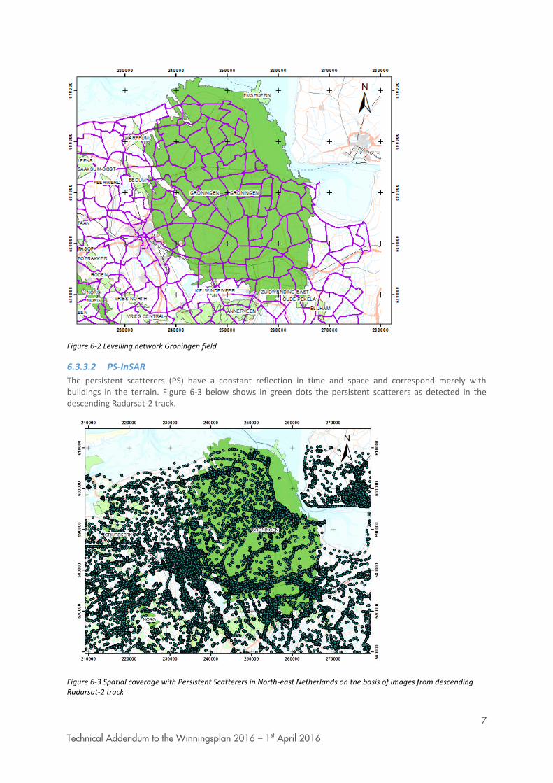
7
Technical Addendum to the Winningsplan 2016 – 1st April 2016
Figure 6-2 Levelling network Groningen field
6.3.3.2 PS-InSAR
The persistent scatterers (PS) have a constant reflection in time and space and correspond merely with buildings in the terrain. Figure 6-3 below shows in green dots the persistent scatterers as detected in the descending Radarsat-2 track.
Figure 6-3 Spatial coverage with Persistent Scatterers in North-east Netherlands on the basis of images from descending Radarsat-2 track
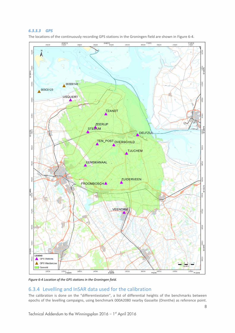
8
Technical Addendum to the Winningsplan 2016 – 1st April 2016
6.3.3.3 GPS
The locations of the continuously recording GPS stations in the Groningen field are shown in Figure 6-4.
Figure 6-4 Location of the GPS stations in the Groningen field.
6.3.4 Levelling and InSAR data used for the calibration The calibration is done on the “differentiestaten”, a list of differential heights of the benchmarks between epochs of the levelling campaigns, using benchmark 000A2080 nearby Gasselte (Drenthe) as reference point.
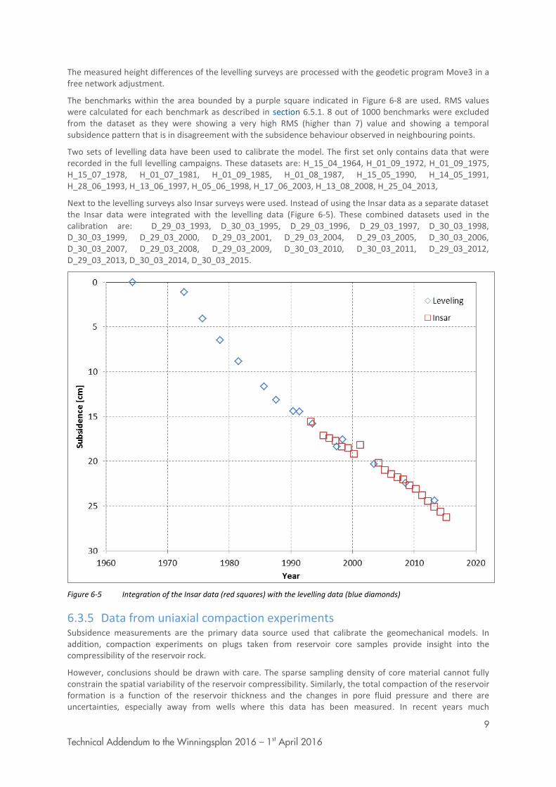
9
Technical Addendum to the Winningsplan 2016 – 1st April 2016
The measured height differences of the levelling surveys are processed with the geodetic program Move3 in a free network adjustment.
The benchmarks within the area bounded by a purple square indicated in Figure 6-8 are used. RMS values were calculated for each benchmark as described in section 6.5.1. 8 out of 1000 benchmarks were excluded from the dataset as they were showing a very high RMS (higher than 7) value and showing a temporal subsidence pattern that is in disagreement with the subsidence behaviour observed in neighbouring points.
Two sets of levelling data have been used to calibrate the model. The first set only contains data that were recorded in the full levelling campaigns. These datasets are: H_15_04_1964, H_01_09_1972, H_01_09_1975, H_15_07_1978, H_01_07_1981, H_01_09_1985, H_01_08_1987, H_15_05_1990, H_14_05_1991, H_28_06_1993, H_13_06_1997, H_05_06_1998, H_17_06_2003, H_13_08_2008, H_25_04_2013,
Next to the levelling surveys also Insar surveys were used. Instead of using the Insar data as a separate dataset the Insar data were integrated with the levelling data (Figure 6-5). These combined datasets used in the calibration are: D_29_03_1993, D_30_03_1995, D_29_03_1996, D_29_03_1997, D_30_03_1998, D_30_03_1999, D_29_03_2000, D_29_03_2001, D_29_03_2004, D_29_03_2005, D_30_03_2006, D_30_03_2007, D_29_03_2008, D_29_03_2009, D_30_03_2010, D_30_03_2011, D_29_03_2012, D_29_03_2013, D_30_03_2014, D_30_03_2015.
Figure 6-5 Integration of the Insar data (red squares) with the levelling data (blue diamonds)
6.3.5 Data from uniaxial compaction experiments Subsidence measurements are the primary data source used that calibrate the geomechanical models. In addition, compaction experiments on plugs taken from reservoir core samples provide insight into the compressibility of the reservoir rock.
However, conclusions should be drawn with care. The sparse sampling density of core material cannot fully constrain the spatial variability of the reservoir compressibility. Similarly, the total compaction of the reservoir formation is a function of the reservoir thickness and the changes in pore fluid pressure and there are uncertainties, especially away from wells where this data has been measured. In recent years much
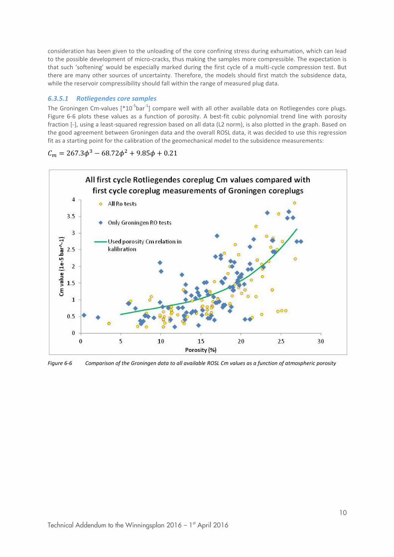
10
Technical Addendum to the Winningsplan 2016 – 1st April 2016
consideration has been given to the unloading of the core confining stress during exhumation, which can lead to the possible development of micro-cracks, thus making the samples more compressible. The expectation is that such ‘softening’ would be especially marked during the first cycle of a multi-cycle compression test. But there are many other sources of uncertainty. Therefore, the models should first match the subsidence data, while the reservoir compressibility should fall within the range of measured plug data.
6.3.5.1 Rotliegendes core samples
The Groningen Cm-values [*10-5
bar-1
] compare well with all other available data on Rotliegendes core plugs. Figure 6-6 plots these values as a function of porosity. A best-fit cubic polynomial trend line with porosity fraction [-], using a least-squared regression based on all data (L2 norm), is also plotted in the graph. Based on the good agreement between Groningen data and the overall ROSL data, it was decided to use this regression fit as a starting point for the calibration of the geomechanical model to the subsidence measurements:
𝐶𝑚 = 267.3𝜙3 − 68.72𝜙2 + 9.85𝜙 + 0.21
Figure 6-6 Comparison of the Groningen data to all available ROSL Cm values as a function of atmospheric porosity
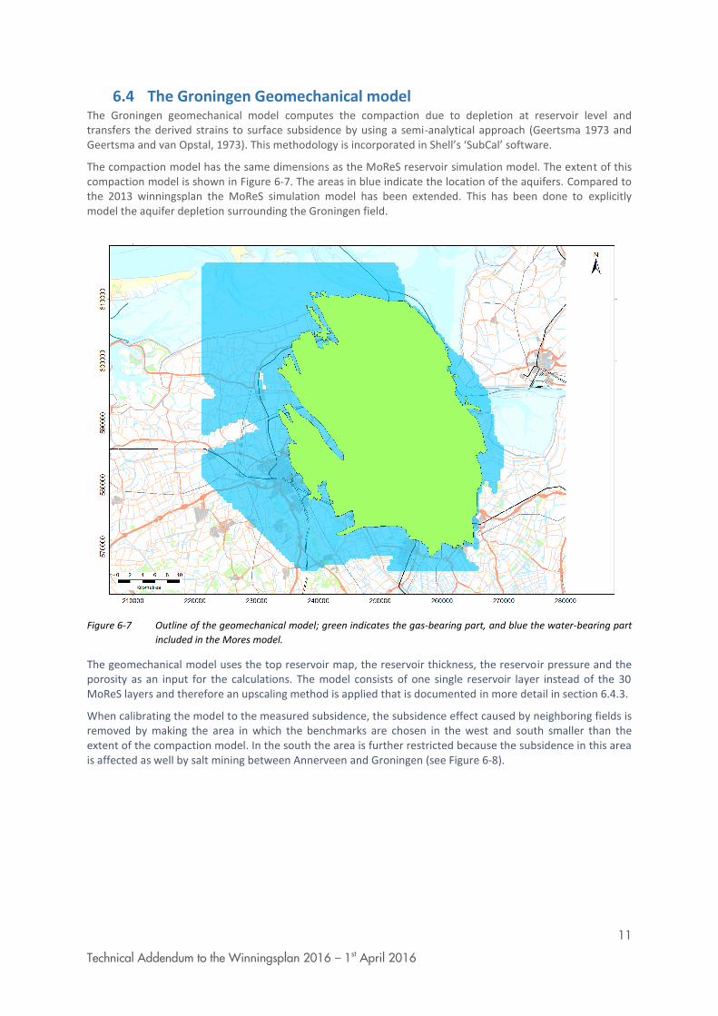
11
Technical Addendum to the Winningsplan 2016 – 1st April 2016
6.4 The Groningen Geomechanical model The Groningen geomechanical model computes the compaction due to depletion at reservoir level and transfers the derived strains to surface subsidence by using a semi-analytical approach (Geertsma 1973 and Geertsma and van Opstal, 1973). This methodology is incorporated in Shell’s ‘SubCal’ software.
The compaction model has the same dimensions as the MoReS reservoir simulation model. The extent of this compaction model is shown in Figure 6-7. The areas in blue indicate the location of the aquifers. Compared to the 2013 winningsplan the MoReS simulation model has been extended. This has been done to explicitly model the aquifer depletion surrounding the Groningen field.
Figure 6-7 Outline of the geomechanical model; green indicates the gas-bearing part, and blue the water-bearing part
included in the Mores model.
The geomechanical model uses the top reservoir map, the reservoir thickness, the reservoir pressure and the porosity as an input for the calculations. The model consists of one single reservoir layer instead of the 30 MoReS layers and therefore an upscaling method is applied that is documented in more detail in section 6.4.3.
When calibrating the model to the measured subsidence, the subsidence effect caused by neighboring fields is removed by making the area in which the benchmarks are chosen in the west and south smaller than the extent of the compaction model. In the south the area is further restricted because the subsidence in this area is affected as well by salt mining between Annerveen and Groningen (see Figure 6-8).
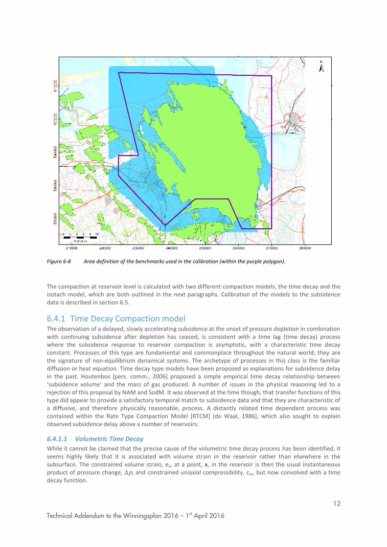
12
Technical Addendum to the Winningsplan 2016 – 1st April 2016
Figure 6-8 Area definition of the benchmarks used in the calibration (within the purple polygon).
The compaction at reservoir level is calculated with two different compaction models, the time-decay and the isotach model, which are both outlined in the next paragraphs. Calibration of the models to the subsidence data is described in section 6.5.
6.4.1 Time Decay Compaction model The observation of a delayed, slowly accelerating subsidence at the onset of pressure depletion in combination with continuing subsidence after depletion has ceased, is consistent with a time lag (time decay) process where the subsidence response to reservoir compaction is asymptotic, with a characteristic time decay constant. Processes of this type are fundamental and commonplace throughout the natural world; they are the signature of non-equilibrium dynamical systems. The archetype of processes in this class is the familiar diffusion or heat equation. Time decay type models have been proposed as explanations for subsidence delay in the past. Houtenbos [pers. comm., 2006] proposed a simple empirical time decay relationship between ‘subsidence volume’ and the mass of gas produced. A number of issues in the physical reasoning led to a rejection of this proposal by NAM and SodM. It was observed at the time though, that transfer functions of this type did appear to provide a satisfactory temporal match to subsidence data and that they are characteristic of a diffusive, and therefore physically reasonable, process. A distantly related time dependent process was contained within the Rate Type Compaction Model [RTCM] (de Waal, 1986), which also sought to explain observed subsidence delay above a number of reservoirs.
6.4.1.1 Volumetric Time Decay
While it cannot be claimed that the precise cause of the volumetric time decay process has been identified, it seems highly likely that it is associated with volume strain in the reservoir rather than elsewhere in the subsurface. The constrained volume strain, eii, at a point, x, in the reservoir is then the usual instantaneous product of pressure change, Δp, and constrained uniaxial compressibility, cm, but now convolved with a time decay function.

13
Technical Addendum to the Winningsplan 2016 – 1st April 2016
𝑒𝑖𝑖(𝐱, 𝑡) = ∆𝑝(𝐱, 𝑡) 𝑐𝑚(𝐱) ∗𝑡 1
𝜏exp [
−𝑡
𝜏]
Here, t, is time, *t, is the convolution operator with respect to time and, τ, is a time decay constant. The best fitting time decay constants for the Groningen field were found by inversion using a semi-analytic geomechanical model and have values of some 3 to 8 years.
It should be realised that it is quite possible that the observed time decay is not a material property of the reservoir rock, but could be due to particularities of the reservoir geometry, pore fluids or some other factor. Therefore it cannot be assumed that the time decay constant appropriate for one reservoir can be applied to another based simply on rock type.
6.4.2 Isotach formulation of the Rate Type Compaction model In the Netherlands, a form of this model is the most accepted model for settlement calculations in soft soil. The model is also known as the a,b,c isotachen model (den Haan, 2003). TNO (2013) investigated the application of this model on cemented rock using the laboratory experiments from de Waal as a starting point (De Waal, 1986). Adjustments of this a, b, c isotachen model led to the definition of the isotach formulation of the rate type compaction model (RTCiM) which was also implemented by NAM and used to calibrate the compaction model and estimate future subsidence. Figure 6-9 shows the Standard Linear Solid (SLS) model, the most simple form of the general isotach model, as a spring-dashpot system (TNO, 2013)
Figure 6-9 Representation of the SLS model
The compaction in the RTCiM model is calculated according the following numerical scheme The simulation is started from the state where effective stress 𝜎′
is equal to reference effective stress 𝜎′𝑟𝑒𝑓, and elastic strain
is equal to the secular strain which are at start (t) zero 𝜀𝑑 = 𝜀𝑠 = 0, 𝑡 = 0 and increases with a fixed time step size 𝛥𝑡. The effective stress as a function of time 𝜎′(𝑡) is known as well as 𝜎′(0) which is given as 𝜎′(0)
=𝜎′𝑟𝑒𝑓 as otherwise 𝜀𝑑 ≠ 0 at t = 0. The compaction is calculated using the following algorithm:
1) Use current 𝜎′ and 𝜀 = 𝜀𝑑 + 𝜀𝑠 and calculate secular strain rate 𝜀�̇� from
𝜀�̇� = (𝜀 − 𝜀0
𝜎′− 𝐶𝑚,𝑎) 𝜎′̇ 𝑟𝑒𝑓 (
𝜀 − 𝜀0
𝜎′𝐶𝑚,𝑟𝑒𝑓
)
−1/𝑏
2) Calculate increase in secular strain 𝛥𝜀𝑠 = 𝜀�̇�𝛥𝑡 and update εs
3) Update 𝑡 = 𝑡 + 𝛥𝑡
4) Calculate direct strain εd from 𝜀𝑑 = 𝐶𝑚,𝑎(𝜎′ − 𝜎𝑟𝑒𝑓′ ) using the new σ’(t)
5) Calculate 𝜀 = 𝜀𝑑 + 𝜀𝑠
After step 5 the algorithm goes back to step 1.
6.4.3 Upscaling of input data The reservoir modelling has been performed using Shell’s reservoir simulator MoReS. It uses a 3-dimensional gridded reservoir structure, which includes porosity and permeability information and attempts to solve for the fluid flow and pressure changes as constrained by historic production and pressure data taken from wells. The reservoir model therefore contains self-consistent porosity and pressure change information that should be used in the geomechanical modeling. However, the reservoir model tends to use a finer grid size than is needed for the geomechanical model so ‘upscaling’ is required.
For the Groningen field, a MoReS reservoir model was built consisting of 30 vertically stacked layers and with grid dimensions of 250 m by 250 m, or less. The reservoir formation in the Geomechanical model is made up of
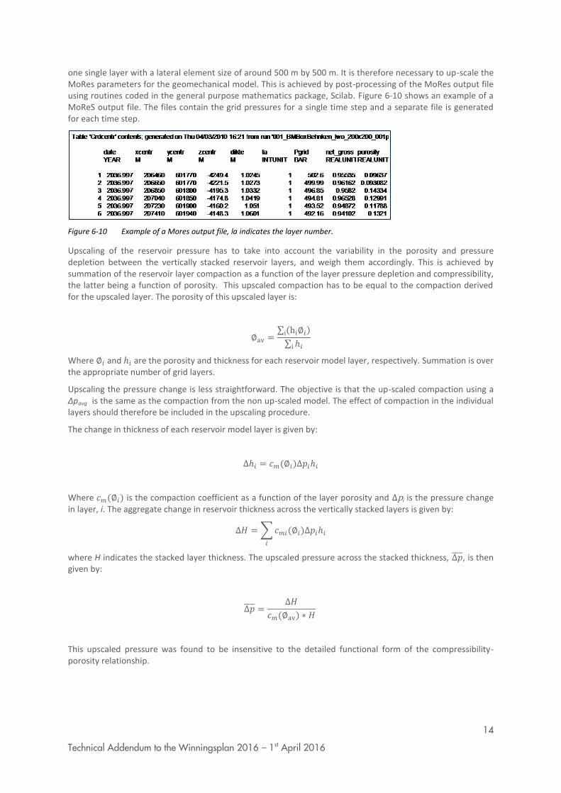
14
Technical Addendum to the Winningsplan 2016 – 1st April 2016
one single layer with a lateral element size of around 500 m by 500 m. It is therefore necessary to up-scale the MoRes parameters for the geomechanical model. This is achieved by post-processing of the MoRes output file using routines coded in the general purpose mathematics package, Scilab. Figure 6-10 shows an example of a MoReS output file. The files contain the grid pressures for a single time step and a separate file is generated for each time step.
Figure 6-10 Example of a Mores output file, la indicates the layer number.
Upscaling of the reservoir pressure has to take into account the variability in the porosity and pressure depletion between the vertically stacked reservoir layers, and weigh them accordingly. This is achieved by summation of the reservoir layer compaction as a function of the layer pressure depletion and compressibility, the latter being a function of porosity. This upscaled compaction has to be equal to the compaction derived for the upscaled layer. The porosity of this upscaled layer is:
∅av =∑ (hi∅𝑖)i
∑ ℎ𝑖i
Where ∅𝑖 and ℎ𝑖 are the porosity and thickness for each reservoir model layer, respectively. Summation is over the appropriate number of grid layers.
Upscaling the pressure change is less straightforward. The objective is that the up-scaled compaction using a Δpavg is the same as the compaction from the non up-scaled model. The effect of compaction in the individual layers should therefore be included in the upscaling procedure.
The change in thickness of each reservoir model layer is given by:
∆ℎ𝑖 = 𝑐𝑚(∅𝑖)∆𝑝𝑖ℎ𝑖
Where 𝑐𝑚(∅𝑖) is the compaction coefficient as a function of the layer porosity and Δpi is the pressure change in layer, i. The aggregate change in reservoir thickness across the vertically stacked layers is given by:
∆𝐻 = ∑ 𝑐𝑚𝑖(∅𝑖)∆𝑝𝑖ℎ𝑖
𝑖
where H indicates the stacked layer thickness. The upscaled pressure across the stacked thickness, ∆𝑝̅̅̅̅ , is then given by:
∆𝑝̅̅̅̅ =∆𝐻
𝑐𝑚(∅av) ∗ 𝐻
This upscaled pressure was found to be insensitive to the detailed functional form of the compressibility-porosity relationship.
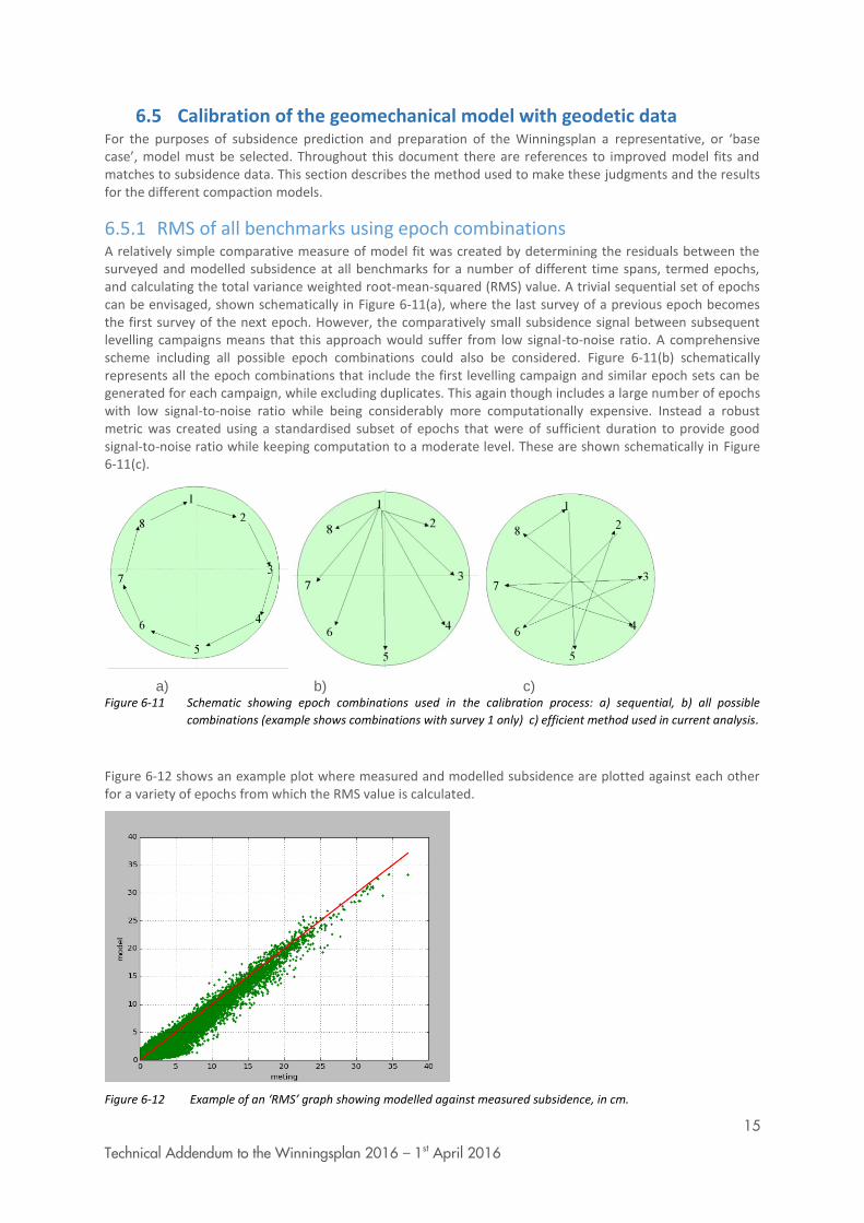
15
Technical Addendum to the Winningsplan 2016 – 1st April 2016
6.5 Calibration of the geomechanical model with geodetic data For the purposes of subsidence prediction and preparation of the Winningsplan a representative, or ‘base case’, model must be selected. Throughout this document there are references to improved model fits and matches to subsidence data. This section describes the method used to make these judgments and the results for the different compaction models.
6.5.1 RMS of all benchmarks using epoch combinations A relatively simple comparative measure of model fit was created by determining the residuals between the surveyed and modelled subsidence at all benchmarks for a number of different time spans, termed epochs, and calculating the total variance weighted root-mean-squared (RMS) value. A trivial sequential set of epochs can be envisaged, shown schematically in Figure 6-11(a), where the last survey of a previous epoch becomes the first survey of the next epoch. However, the comparatively small subsidence signal between subsequent levelling campaigns means that this approach would suffer from low signal-to-noise ratio. A comprehensive scheme including all possible epoch combinations could also be considered. Figure 6-11(b) schematically represents all the epoch combinations that include the first levelling campaign and similar epoch sets can be generated for each campaign, while excluding duplicates. This again though includes a large number of epochs with low signal-to-noise ratio while being considerably more computationally expensive. Instead a robust metric was created using a standardised subset of epochs that were of sufficient duration to provide good signal-to-noise ratio while keeping computation to a moderate level. These are shown schematically in Figure 6-11(c).
a) b) c) Figure 6-11 Schematic showing epoch combinations used in the calibration process: a) sequential, b) all possible
combinations (example shows combinations with survey 1 only) c) efficient method used in current analysis.
Figure 6-12 shows an example plot where measured and modelled subsidence are plotted against each other for a variety of epochs from which the RMS value is calculated.
Figure 6-12 Example of an ‘RMS’ graph showing modelled against measured subsidence, in cm.

16
Technical Addendum to the Winningsplan 2016 – 1st April 2016
6.5.2 Winningsplan 2013 spatial fit In the Winningsplan 2013 the compaction was based on a porosity-Cm relation, which implies that the subsidence will be biased by a (non-unique) porosity distribution based on expert judgment by the geologist. This method showed an under prediction of the subsidence in the south of the field while the model over predicted the measured subsidence in the north (Figure 6-13). This questions the use of such strict coupling between the porosity and the compressibility of the rock. The large scatter in the laboratory measurements as pointed out in Figure 6-6 further supports this.
Figure 6-13 Difference between measured and modelled subsidence since start production for the Winningplan 2013
model.
In the current Winningsplan 2016 the spatial subsidence fit was improved by inverting to a spatially varying Cm grid with a grid size of 1x1 km
2. However inverting to the Cm value does not give a unique solution and can
return large spatial scattering of the Cm. To reduce this scatter the inversion was regularized by using the Cm porosity relation (used in the Winningsplan 2013) as a prior. In the inversion process penalties were put on:
1. The difference between the inverted Cm and porosity derived Cm 2. The residuals between modelled and measured subsidence.
This resulting Cm grid is shown in Figure 6-14 and has been used for both the time decay and RTCiM model. In Figure 6-15 both the laboratory measured and the inverted Cm values are shown as function of porosity. To obtain an optimal subsidence fit in time for the different compaction models a multiplication factor was applied to the Cm grid obtained from the inversion.
In the next paragraphs the results are discussed in more detail for the various compaction models.

17
Technical Addendum to the Winningsplan 2016 – 1st April 2016
Figure 6-14 Cm (* 10-5
bar-1
) for Groningen calculated from inversion to subsidence
Figure 6-15 Cm porosity plot including the inverted Cm values for the Time decay model

18
Technical Addendum to the Winningsplan 2016 – 1st April 2016
6.5.3 Time Decay model The calibration of the time decay model resulted in the following parameters for the time decay compaction model:
Cm multiplication factor is 0.94
decay time 𝜏: 3 year
The difference between the measured and modelled subsidence between first and last measurement (2013) is shown in Figure 6-16. Note that the subsidence calculation has been done only for Groningen, other fields were not included in this calculation and therefore the difference between modeled and measured subsidence is increasing near the neighboring fields. The figure shows that the values for the residuals between model and observed data are very low.
Figure 6-16 Time decay model: Difference between measured and modelled subsidence from start production/ first
measurement until end 2013.
To investigate the uniqueness of the time decay parameters, a Monte Carlo simulation was carried out. The results of this analysis are shown in Figure 6-17. In this figure, the Cm multiplication factors are plotted against the decay times (in years) and the colors indicate the RMS value. This figure show a narrow bandwidth for the Cm but a wider bandwidth for the decay time 𝜏.
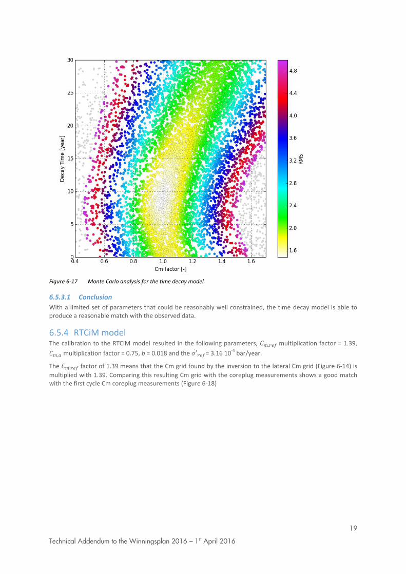
19
Technical Addendum to the Winningsplan 2016 – 1st April 2016
Figure 6-17 Monte Carlo analysis for the time decay model.
6.5.3.1 Conclusion
With a limited set of parameters that could be reasonably well constrained, the time decay model is able to produce a reasonable match with the observed data.
6.5.4 RTCiM model The calibration to the RTCiM model resulted in the following parameters, 𝐶𝑚,𝑟𝑒𝑓 multiplication factor = 1.39,
𝐶𝑚,𝑎 multiplication factor = 0.75, b = 0.018 and the 𝜎′̇ 𝑟𝑒𝑓= 3.16 10-4
bar/year.
The 𝐶𝑚,𝑟𝑒𝑓 factor of 1.39 means that the Cm grid found by the inversion to the lateral Cm grid (Figure 6-14) is
multiplied with 1.39. Comparing this resulting Cm grid with the coreplug measurements shows a good match with the first cycle Cm coreplug measurements (Figure 6-18)

20
Technical Addendum to the Winningsplan 2016 – 1st April 2016
Figure 6-18 Core plug and inverted Cm for the RTCiM model
The spatial fit of this model is shown in Figure 6-19, in this plot the difference between modelled and measured subsidence is shown for the period 1972 – 2013. The figure shows that the values for the residuals between model and observed data are very low.
Figure 6-19 RTCiM: Difference between measured and modelled subsidence from start production/ first measurement
until end 2013
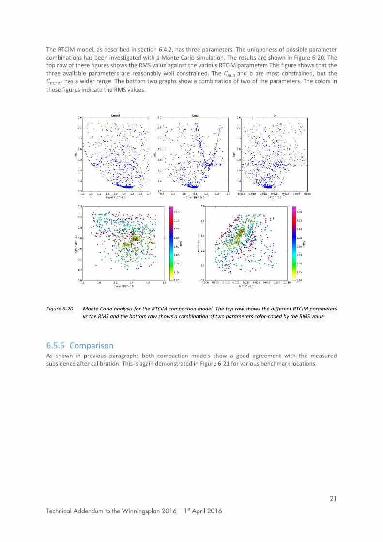
21
Technical Addendum to the Winningsplan 2016 – 1st April 2016
The RTCiM model, as described in section 6.4.2, has three parameters. The uniqueness of possible parameter combinations has been investigated with a Monte Carlo simulation. The results are shown in Figure 6-20. The top row of these figures shows the RMS value against the various RTCiM parameters This figure shows that the three available parameters are reasonably well constrained. The 𝐶𝑚,𝑎 and b are most constrained, but the 𝐶𝑚,𝑟𝑒𝑓 has a wider range. The bottom two graphs show a combination of two of the parameters. The colors in
these figures indicate the RMS values.
Figure 6-20 Monte Carlo analysis for the RTCiM compaction model. The top row shows the different RTCiM parameters
vs the RMS and the bottom row shows a combination of two parameters color-coded by the RMS value
6.5.5 Comparison As shown in previous paragraphs both compaction models show a good agreement with the measured subsidence after calibration. This is again demonstrated in Figure 6-21 for various benchmark locations.
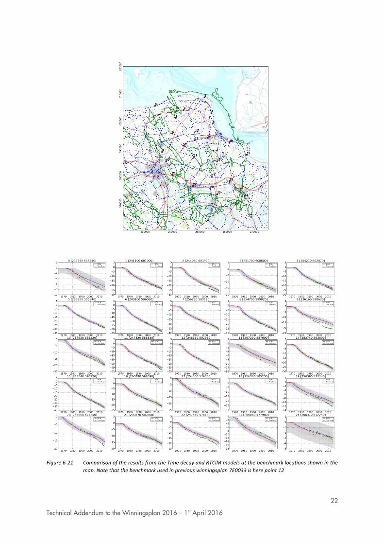
22
Technical Addendum to the Winningsplan 2016 – 1st April 2016
Figure 6-21 Comparison of the results from the Time decay and RTCiM models at the benchmark locations shown in the
map. Note that the benchmark used in previous winningsplan 7E0033 is here point 12

23
Technical Addendum to the Winningsplan 2016 – 1st April 2016
6.6 RTCiM and Time Decay response to changes in production To mitigate seismicity the gas production of Groningen was restricted. Noticeably the volumes of the production clusters in the north of the field were lowered. This resulted in a spatial redistribution of the production and depletion. The effect on subsidence is shown in Figure 6-22. The top row shows the subsidence at benchmark locations (using InSAR interpolation) for the period before (2010 -2012) and after (2013 – 2015) the production change. It can be observed that the higher subsidence values shifted to the south of the field. Note that the change in the subsidence pattern is about 5 mm, which is about the noise level.
Figure 6-22 Change in subsidence pattern before and after the production change in 2013. Top row: measured subsidence. Bottom row: comparison between time decay and RTCiM model results (Subsidence in cm).
The bottom row shows the subsidence realizations for the RTCiM and time decay model for the same periods of time. The observed shift of the subsidence pattern to the south is reproduced best with the RTCiM model. Note that the RTCiM model does not cover the Bedum field in the North West, which shows about 1 cm of subsidence in the time decay model.
6.6.1 Selection of base case compaction model Both the Time decay and the RTCiM compaction models result in a good overall fit to the observed subsidence data above the Groningen field.
The RTCiM compaction model is chosen as the base case compaction model because it results in the best fit to the temporal and spatial observed response of the subsidence to production changes.
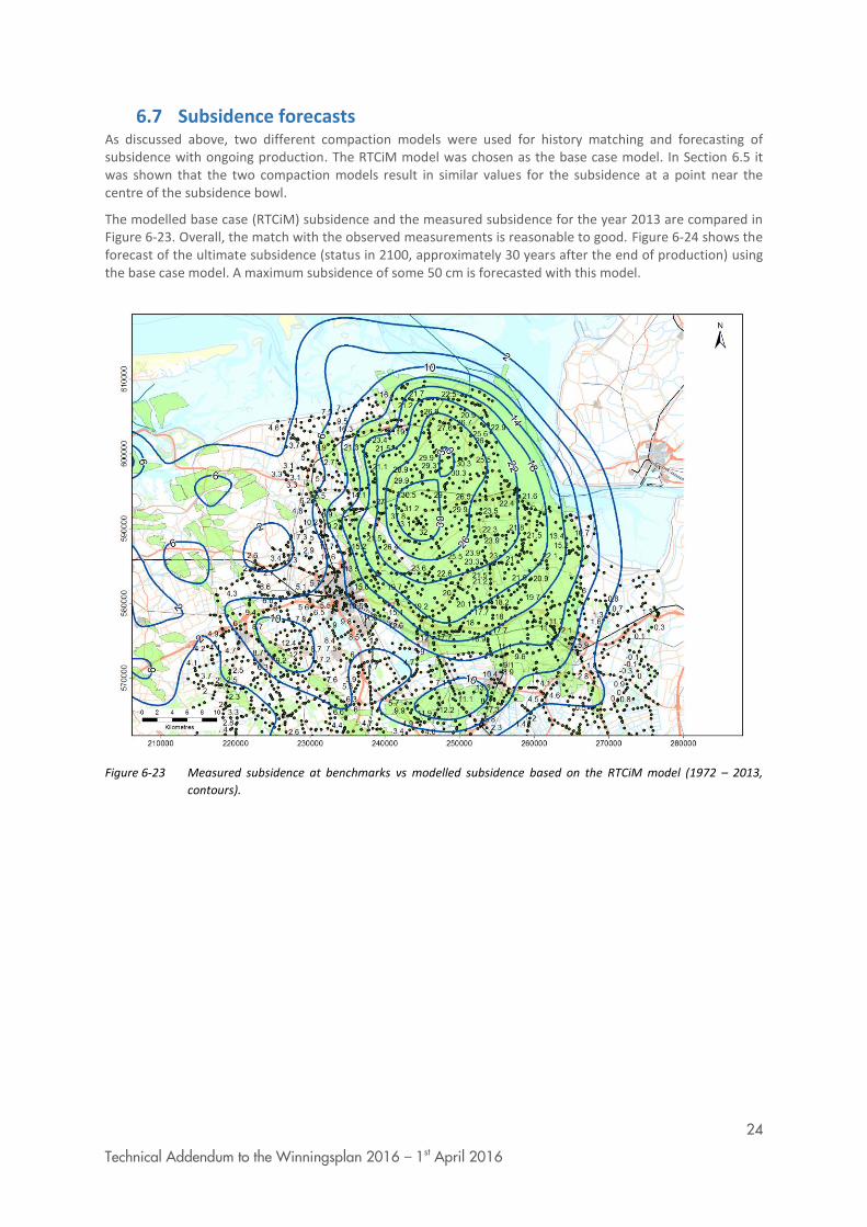
24
Technical Addendum to the Winningsplan 2016 – 1st April 2016
6.7 Subsidence forecasts As discussed above, two different compaction models were used for history matching and forecasting of subsidence with ongoing production. The RTCiM model was chosen as the base case model. In Section 6.5 it was shown that the two compaction models result in similar values for the subsidence at a point near the centre of the subsidence bowl.
The modelled base case (RTCiM) subsidence and the measured subsidence for the year 2013 are compared in Figure 6-23. Overall, the match with the observed measurements is reasonable to good. Figure 6-24 shows the forecast of the ultimate subsidence (status in 2100, approximately 30 years after the end of production) using the base case model. A maximum subsidence of some 50 cm is forecasted with this model.
Figure 6-23 Measured subsidence at benchmarks vs modelled subsidence based on the RTCiM model (1972 – 2013,
contours).

25
Technical Addendum to the Winningsplan 2016 – 1st April 2016
Figure 6-24 Subsidence prognosis based on the RTCiM model in 2100, approximately 30 years after the end of gas
production. This figure shows the subsidence due to gas production for the Groningen field in combination
with the subsidence predicted for other fields (subsidence in cm).
The development of the future subsidence through time for the different compaction models and different (optimized) gas production scenarios is shown in Figure 6-25 to Figure 6-28.
The RTCiM model reacts faster to changes in reservoir pressure than the time decay model. The Cm is also somewhat higher which leads to higher subsidence values. Compared to the “Statusreport 2015 (NAM, 2015)”, in which the time decay model was used as the base case, the RTCiM model predicts an additional 4 cm subsidence in the deepest point at end of field life.
2016-2020 2016-2025 2016-2065
Figure 6-25 Development of future subsidence according to the time decay compaction model with 27 BCM annual
production

26
Technical Addendum to the Winningsplan 2016 – 1st April 2016
2016-2020 2016-2025 2016-2065
Figure 6-26 Development of future subsidence according to the time decay compaction model with 33 BCM annual
production
2016-2020 2016-2025 2016-2065
Figure 6-27 Development of future subsidence according to the RTCiM model with 27 BCM annual production
2016-2020 2016-2025 2016-2065
Figure 6-28 Development of future subsidence according to the RTCiM model with 33 BCM annual production

27
Technical Addendum to the Winningsplan 2016 – 1st April 2016
Figure 6-29 shows the results of subsidence models in comparison with the measured subsidence at benchmark 007E0033 near the deepest point of the subsidence bowl.
The parameters used in model realisation A give the best fit with the measurements over the entire time period. The parameters used for realisation B give a reasonable fit, but generally overestimate the measurements and can be considered as the possible upper limit of model realisations. The quality of fit of the models to the data is determined from the fit at all benchmarks.
This spread of models and parameters sufficiently reflects the uncertainty bandwidth of the subsidence forecasts (about 20%). The RTCiM model predicts more subsidence than the Time Decay model (after the end of production). The RTCiM A model was used as basis for the winningsplan. In order to reduce the uncertainty in the future, the subsidence will be monitored closely as described earlier.
Figure 6-29 Development of subsidence in time at benchmark 007E0033 near the centre of the subsidence bowl.
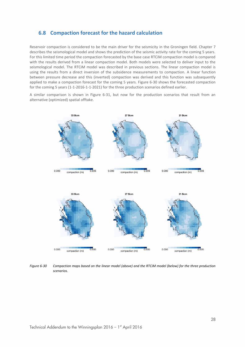
28
Technical Addendum to the Winningsplan 2016 – 1st April 2016
6.8 Compaction forecast for the hazard calculation
Reservoir compaction is considered to be the main driver for the seismicity in the Groningen field. Chapter 7 describes the seismological model and shows the prediction of the seismic activity rate for the coming 5 years. For this limited time period the compaction forecasted by the base case RTCiM compaction model is compared with the results derived from a linear compaction model. Both models were selected to deliver input to the seismological model. The RTCiM model was described in previous sections. The linear compaction model is using the results from a direct inversion of the subsidence measurements to compaction. A linear function between pressure decrease and this (inverted) compaction was derived and this function was subsequently applied to make a compaction forecast for the coming 5 years. Figure 6-30 shows the forecasted compaction for the coming 5 years (1-1-2016-1-1-2021) for the three production scenarios defined earlier.
A similar comparison is shown in Figure 6-31, but now for the production scenarios that result from an alternative (optimized) spatial offtake.
Figure 6-30 Compaction maps based on the linear model (above) and the RTCiM model (below) for the three production
scenarios.
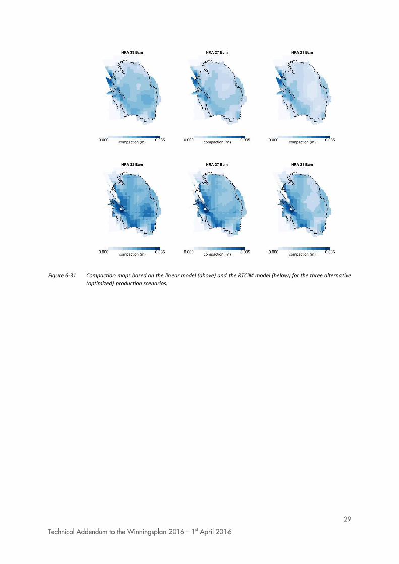
29
Technical Addendum to the Winningsplan 2016 – 1st April 2016
Figure 6-31 Compaction maps based on the linear model (above) and the RTCiM model (below) for the three alternative
(optimized) production scenarios.

1
Technical Addendum to the Winningsplan 2016 – 1st April 2016
Technical Addendum to the Winningsplan Groningen 2016 Production, Subsidence, Induced Earthquakes and Seismic Hazard and Risk Assessment in the Groningen Field PART III Hazard

2
Technical Addendum to the Winningsplan 2016 – 1st April 2016
The report “Technical Addendum to the Winningsplan Groningen 2016 - Production, Subsidence, Induced Earthquakes and Seismic Hazard and Risk Assessment in the Groningen Field” consists of five separate documents:
Document 1 Chapters 1 to 5; Summary and Production
Document 2 Chapter 6; Subsidence
Document 3 Chapter 7; Hazard
Document 4 Chapter 8; Risk
Document 5 Chapter 9; Damage and Appendices.
Each of these documents is also available as a *.pdf file of a size smaller than 10Mbyte, allowing sharing through e-mail.
© EP201603238413 Dit rapport is een weerslag van een voortdurend studie- en dataverzamelingsprogramma en bevat de stand der kennis van april 2016. Het copyright van dit rapport ligt bij de Nederlandse Aardolie Maatschappij B.V. Het copyright van de onderliggende studies berust bij de respectievelijke auteurs. Dit rapport of delen daaruit mogen alleen met een nadrukkelijke status-en bronvermelding worden overgenomen of gepubliceerd.
3
Technical Addendum to the Winningsplan 2016 – 1st April 2016
Contents 7 Hazard Assessment ......................................................................................................................... 4
Hazard Metric ..................................................................................................................................... 4
Peak Ground Acceleration 4
Probabilistic Hazard Assessment ........................................................................................................ 6
Seismic Event Rate and Total Seismic Moment Rate with time 6
Ground Acceleration incorporating Local Site Effects 13
Hazard Logic Tree 16
Hazard Assessment 17
Disaggregation of Seismic Hazard 23
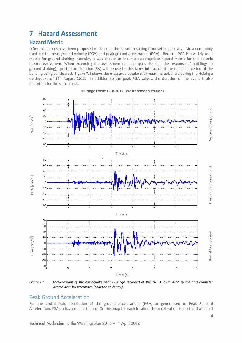
4
Technical Addendum to the Winningsplan 2016 – 1st April 2016
7 Hazard Assessment Hazard Metric Different metrics have been proposed to describe the hazard resulting from seismic activity. Most commonly used are the peak ground velocity (PGV) and peak ground acceleration (PGA). Because PGA is a widely used metric for ground shaking intensity, it was chosen as the most appropriate hazard metric for this seismic hazard assessment. When extending the assessment to encompass risk (i.e. the response of buildings to ground shaking), spectral acceleration (SA) will be used – this takes into account the response period of the building being considered. Figure 7.1 shows the measured acceleration near the epicentre during the Huizinge earthquake of 16
th August 2012. In addition to the peak PGA values, the duration of the event is also
important for the seismic risk.
Huizinge Event 16-8-2012 (Westeremden station)
PG
A [
cm/s
2]
Ver
tica
l Co
mp
on
ent
Time [s]
PG
A [
cm/s
2]
Tr
ansv
erse
Co
mp
on
ent
Time [s]
PG
A [
cm/s
2]
Rad
ial C
om
po
nen
t
Time [s]
Figure 7.1 Accelerogram of the earthquake near Huizinge recorded at the 16th
August 2012 by the accelerometer
located near Westeremden (near the epicentre).
Peak Ground Acceleration For the probabilistic description of the ground accelerations (PGA, or generalised to Peak Spectral Acceleration, PSA), a hazard map is used. On this map for each location the acceleration is plotted that could
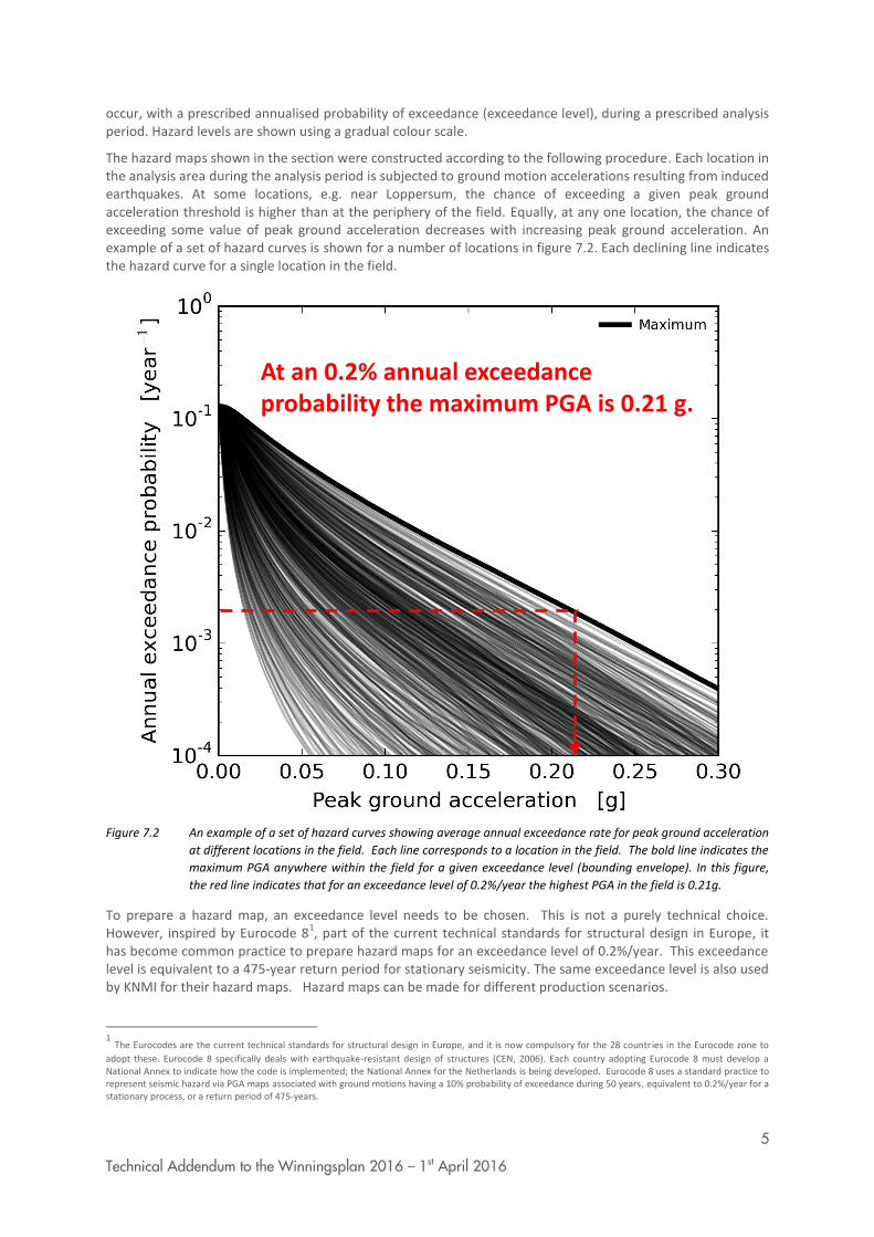
5
Technical Addendum to the Winningsplan 2016 – 1st April 2016
occur, with a prescribed annualised probability of exceedance (exceedance level), during a prescribed analysis period. Hazard levels are shown using a gradual colour scale.
The hazard maps shown in the section were constructed according to the following procedure. Each location in the analysis area during the analysis period is subjected to ground motion accelerations resulting from induced earthquakes. At some locations, e.g. near Loppersum, the chance of exceeding a given peak ground acceleration threshold is higher than at the periphery of the field. Equally, at any one location, the chance of exceeding some value of peak ground acceleration decreases with increasing peak ground acceleration. An example of a set of hazard curves is shown for a number of locations in figure 7.2. Each declining line indicates the hazard curve for a single location in the field.
Figure 7.2 An example of a set of hazard curves showing average annual exceedance rate for peak ground acceleration
at different locations in the field. Each line corresponds to a location in the field. The bold line indicates the
maximum PGA anywhere within the field for a given exceedance level (bounding envelope). In this figure,
the red line indicates that for an exceedance level of 0.2%/year the highest PGA in the field is 0.21g.
To prepare a hazard map, an exceedance level needs to be chosen. This is not a purely technical choice. However, inspired by Eurocode 8
1, part of the current technical standards for structural design in Europe, it
has become common practice to prepare hazard maps for an exceedance level of 0.2%/year. This exceedance level is equivalent to a 475-year return period for stationary seismicity. The same exceedance level is also used by KNMI for their hazard maps. Hazard maps can be made for different production scenarios.
1 The Eurocodes are the current technical standards for structural design in Europe, and it is now compulsory for the 28 countries in the Eurocode zone to
adopt these. Eurocode 8 specifically deals with earthquake-resistant design of structures (CEN, 2006). Each country adopting Eurocode 8 must develop a National Annex to indicate how the code is implemented; the National Annex for the Netherlands is being developed. Eurocode 8 uses a standard practice to represent seismic hazard via PGA maps associated with ground motions having a 10% probability of exceedance during 50 years, equivalent to 0.2%/year for a stationary process, or a return period of 475-years.
At an 0.2% annual exceedance probability the maximum PGA is 0.21 g.

6
Technical Addendum to the Winningsplan 2016 – 1st April 2016
Probabilistic Hazard Assessment
Seismic Event Rate and Total Seismic Moment Rate with time Starting at the first step of the causal chain, from gas production via the resulting compaction, seismicity can be assessed. Seismicity is interpreted in this context as the event rate density of earthquakes larger than M ≥ 1.5 and the frequency-magnitude distribution characterised by its slope (b-value) and upper bound (Mmax). This minimum earthquake magnitude of M = 1.5 corresponds to the minimum magnitude of an earthquake, which the installed KNMI geophone network was historically able to record reliably (independent of its location within the field boundary or time of day). Earthquakes with smaller magnitude may not always be detected, because the signal may not be distinguished from the background noise.
Figure 7.3 Expected annual event density maps over from 1995 to 2020 according to the seismological model. The
forecast period is based on the production plan for 33 bcm/year and the linear compaction model. Grey dots
denote the observed epicenters of M ≥ 1.5 events.
Expected event density maps for the period from 2016 to 2020 for various combinations of annual production volume, distribution of production over the field and compaction model are shown in figures 7.4A, 7.4B, and 7.4C. As the event density maps through time are very similar for the linear and RTCiM compaction models, the event density used for the hazard and risk assessment in the winningsplan 2016 is based on compaction calculated using the linear compaction model.
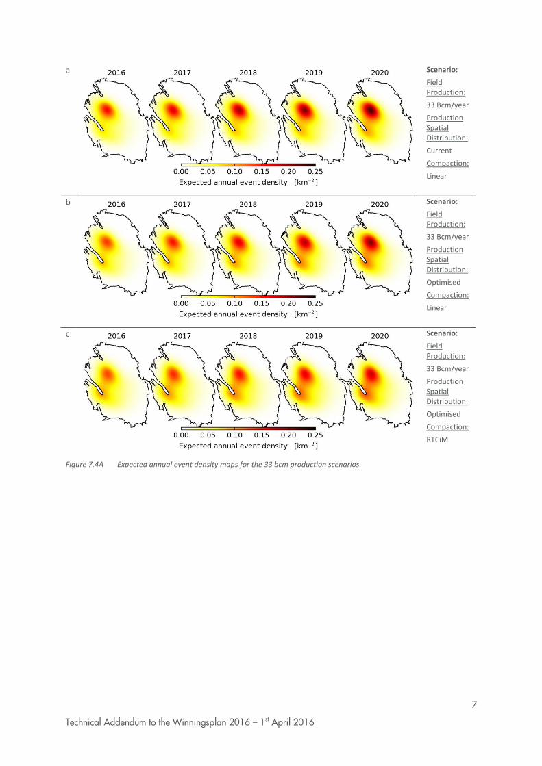
7
Technical Addendum to the Winningsplan 2016 – 1st April 2016
a
Scenario:
Field Production:
33 Bcm/year
Production Spatial Distribution:
Current
Compaction:
Linear
b
Scenario:
Field Production:
33 Bcm/year
Production Spatial Distribution:
Optimised
Compaction:
Linear
c
Scenario:
Field Production:
33 Bcm/year
Production Spatial Distribution:
Optimised
Compaction:
RTCiM
Figure 7.4A Expected annual event density maps for the 33 bcm production scenarios.

8
Technical Addendum to the Winningsplan 2016 – 1st April 2016
a
Scenario:
Field Production:
27 Bcm/year
Production Spatial Distribution:
Current
Compaction:
Linear
b
Scenario:
Field Production:
27 Bcm/year
Production Spatial Distribution:
Optimised
Compaction:
Linear
c
Scenario:
Field Production:
27 Bcm/year
Production Spatial Distribution:
Optimised
Compaction:
RTCiM
Figure 7.4B Expected annual event density maps for the 27 bcm production scenarios.
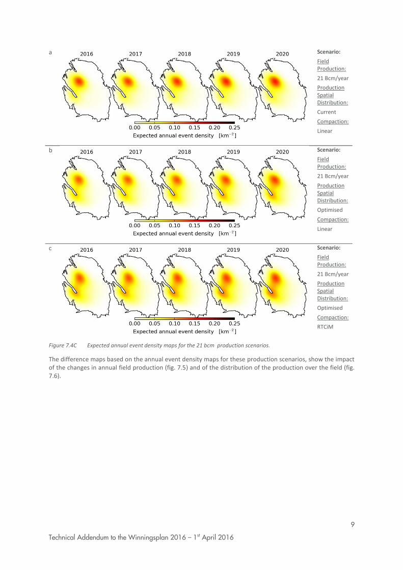
9
Technical Addendum to the Winningsplan 2016 – 1st April 2016
a
Scenario:
Field Production:
21 Bcm/year
Production Spatial Distribution:
Current
Compaction:
Linear
b
Scenario:
Field Production:
21 Bcm/year
Production Spatial Distribution:
Optimised
Compaction:
Linear
c
Scenario:
Field Production:
21 Bcm/year
Production Spatial Distribution:
Optimised
Compaction:
RTCiM
Figure 7.4C Expected annual event density maps for the 21 bcm production scenarios.
The difference maps based on the annual event density maps for these production scenarios, show the impact of the changes in annual field production (fig. 7.5) and of the distribution of the production over the field (fig. 7.6).
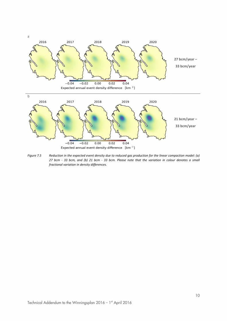
10
Technical Addendum to the Winningsplan 2016 – 1st April 2016
a
27 bcm/year –
33 bcm/year
b
21 bcm/year –
33 bcm/year
Figure 7.5 Reduction in the expected event density due to reduced gas production for the linear compaction model: (a)
27 bcm - 33 bcm, and (b) 21 bcm - 33 bcm. Please note that the variation in colour denotes a small
fractional variation in density differences.
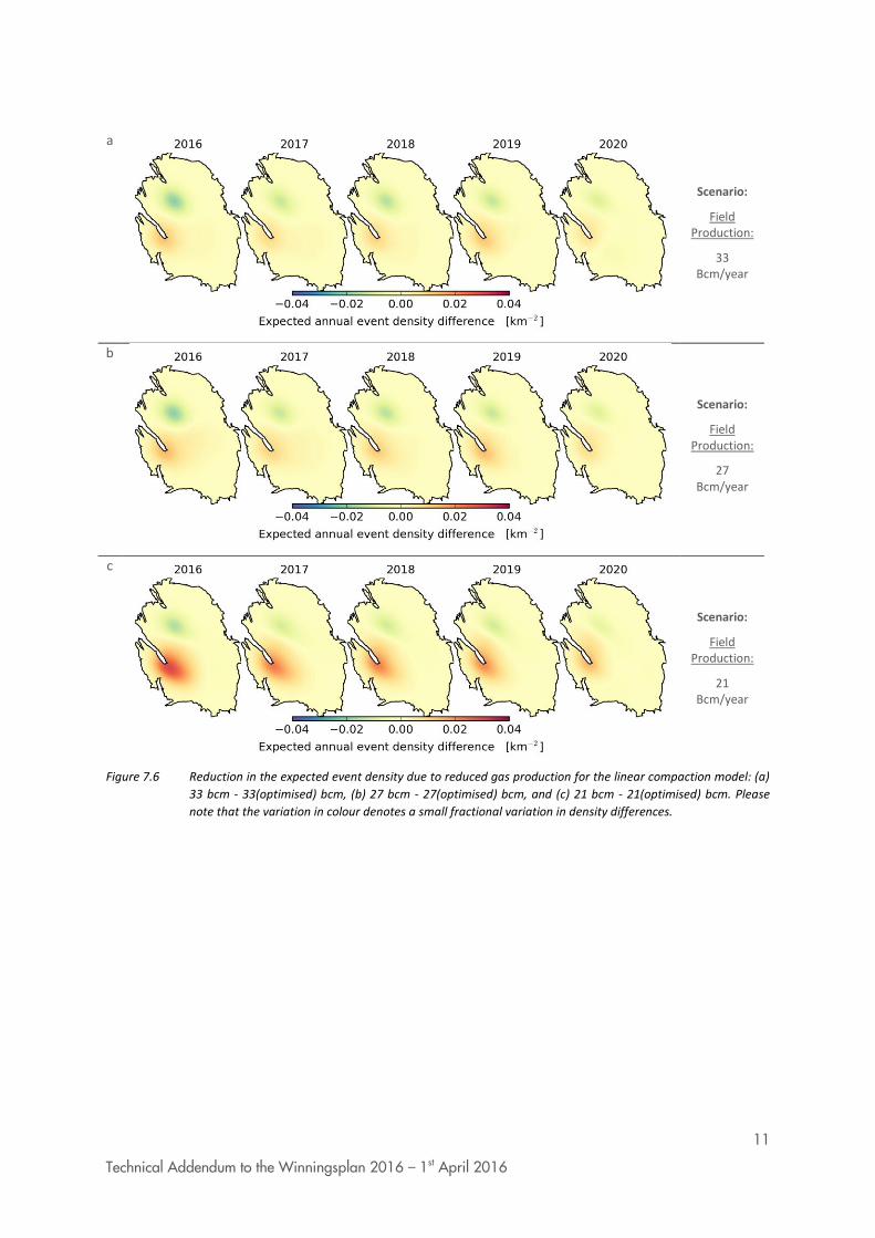
11
Technical Addendum to the Winningsplan 2016 – 1st April 2016
a
Scenario:
Field Production:
33 Bcm/year
b
Scenario:
Field Production:
27 Bcm/year
c
Scenario:
Field Production:
21 Bcm/year
Figure 7.6 Reduction in the expected event density due to reduced gas production for the linear compaction model: (a)
33 bcm - 33(optimised) bcm, (b) 27 bcm - 27(optimised) bcm, and (c) 21 bcm - 21(optimised) bcm. Please
note that the variation in colour denotes a small fractional variation in density differences.
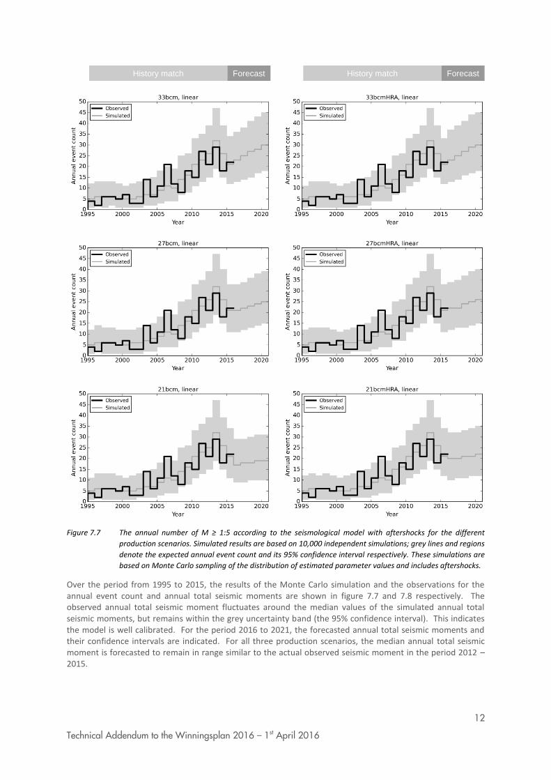
12
Technical Addendum to the Winningsplan 2016 – 1st April 2016
Figure 7.7 The annual number of M ≥ 1:5 according to the seismological model with aftershocks for the different
production scenarios. Simulated results are based on 10,000 independent simulations; grey lines and regions
denote the expected annual event count and its 95% confidence interval respectively. These simulations are
based on Monte Carlo sampling of the distribution of estimated parameter values and includes aftershocks.
Over the period from 1995 to 2015, the results of the Monte Carlo simulation and the observations for the annual event count and annual total seismic moments are shown in figure 7.7 and 7.8 respectively. The observed annual total seismic moment fluctuates around the median values of the simulated annual total seismic moments, but remains within the grey uncertainty band (the 95% confidence interval). This indicates the model is well calibrated. For the period 2016 to 2021, the forecasted annual total seismic moments and their confidence intervals are indicated. For all three production scenarios, the median annual total seismic moment is forecasted to remain in range similar to the actual observed seismic moment in the period 2012 – 2015.
History match Forecast History match Forecast
P97.5
P50
P2.5
P97.5
P50
P2.5
P97.5
P50
P2.5
P97.5
P50
P2.5
History match Forecast History match Forecast
P97.5
P50
P2.5
P97.5
P50
P2.5
P97.5
P50
P2.5
P97.5
P50
P2.5
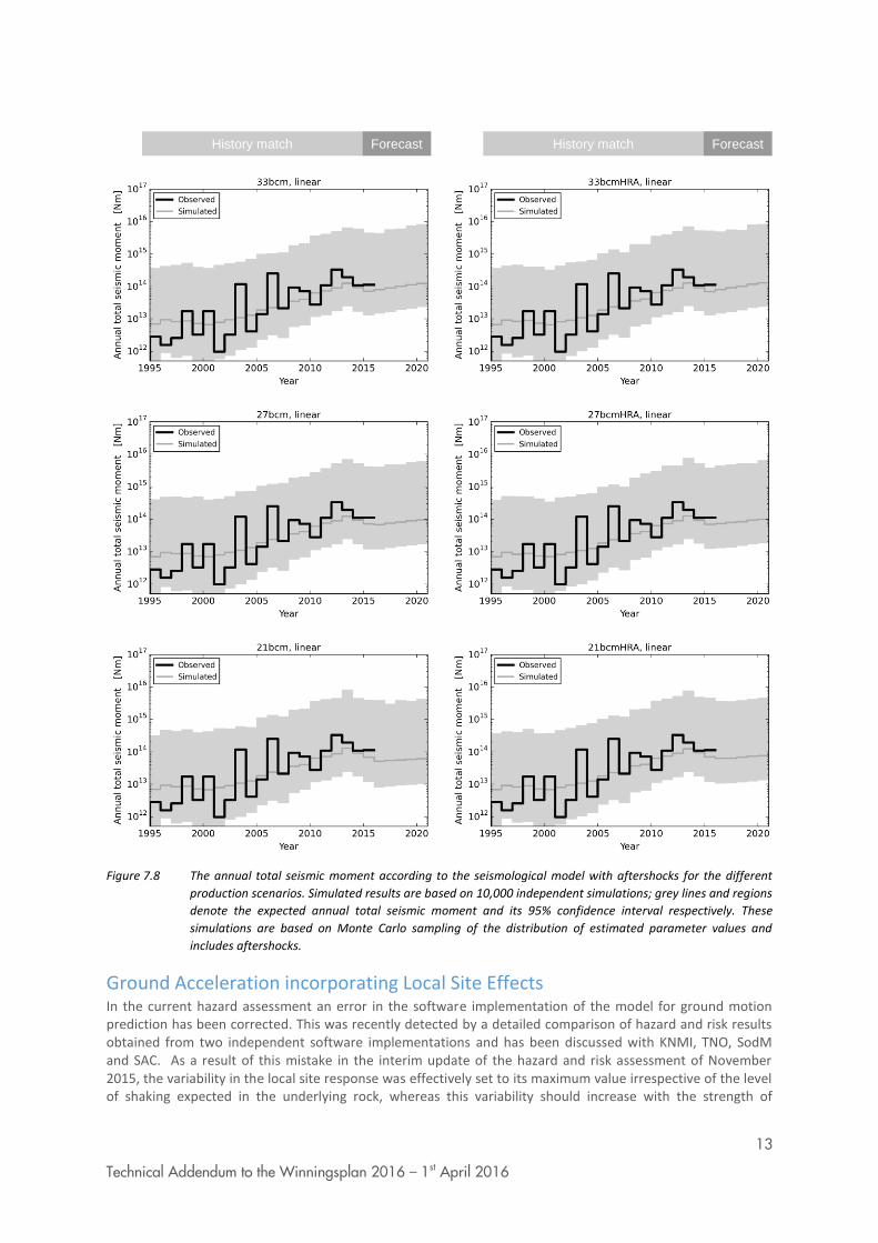
13
Technical Addendum to the Winningsplan 2016 – 1st April 2016
Figure 7.8 The annual total seismic moment according to the seismological model with aftershocks for the different
production scenarios. Simulated results are based on 10,000 independent simulations; grey lines and regions
denote the expected annual total seismic moment and its 95% confidence interval respectively. These
simulations are based on Monte Carlo sampling of the distribution of estimated parameter values and
includes aftershocks.
Ground Acceleration incorporating Local Site Effects In the current hazard assessment an error in the software implementation of the model for ground motion prediction has been corrected. This was recently detected by a detailed comparison of hazard and risk results obtained from two independent software implementations and has been discussed with KNMI, TNO, SodM and SAC. As a result of this mistake in the interim update of the hazard and risk assessment of November 2015, the variability in the local site response was effectively set to its maximum value irrespective of the level of shaking expected in the underlying rock, whereas this variability should increase with the strength of
History match Forecast History match Forecast
P97.5
P50
P2.5
P97.5
P50
P2.5
P97.5
P50
P2.5
P97.5
P50
P2.5
History match Forecast History match Forecast
P97.5
P50
P2.5
P97.5
P50
P2.5
P97.5
P50
P2.5
P97.5
P50
P2.5
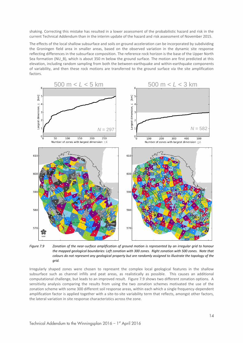
14
Technical Addendum to the Winningsplan 2016 – 1st April 2016
shaking. Correcting this mistake has resulted in a lower assessment of the probabilistic hazard and risk in the current Technical Addendum than in the interim update of the hazard and risk assessment of November 2015.
The effects of the local shallow subsurface and soils on ground acceleration can be incorporated by subdividing the Groningen field area in smaller areas, based on the observed variation in the dynamic site response reflecting differences in the subsurface composition. The reference rock horizon is the base of the Upper North Sea formation (NU_B), which is about 350 m below the ground surface. The motion are first predicted at this elevation, including random sampling from both the between-earthquake and within-earthquake components of variability, and then these rock motions are transferred to the ground surface via the site amplification factors.
Figure 7.9 Zonation of the near-surface amplification of ground motion is represented by an irregular grid to honour
the mapped geological boundaries: Left zonation with 300 zones. Right zonation with 500 zones. Note that
colours do not represent any geological property but are randomly assigned to illustrate the topology of the
grid.
Irregularly shaped zones were chosen to represent the complex local geological features in the shallow subsurface such as channel infills and peat areas, as realistically as possible. This causes an additional computational challenge, but leads to an improved result. Figure 7.9 shows two different zonation options. A sensitivity analysis comparing the results from using the two zonation schemes motivated the use of the zonation scheme with some 300 different soil response areas, within each which a single frequency-dependent amplification factor is applied together with a site-to-site variability term that reflects, amongst other factors, the lateral variation in site response characteristics across the zone.
500 m < L < 5 km
N = 297
500 m < L < 3 km
N = 582
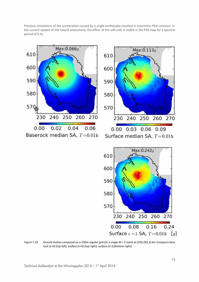
15
Technical Addendum to the Winningsplan 2016 – 1st April 2016
Previous simulations of the acceleration caused by a single earthquake resulted in concentric PGA contours. In the current update of the hazard assessment, the effect of the soft soils is visible in the PSA map for a spectral period of 0.3s.
Figure 7.10 Ground motion computed on a 250m regular grid for a single M = 5 event at (245,595,3) km Compares base
rock (ε=0) (top left), surface (ε=0) (top right), surface (ε=1)(bottom right).
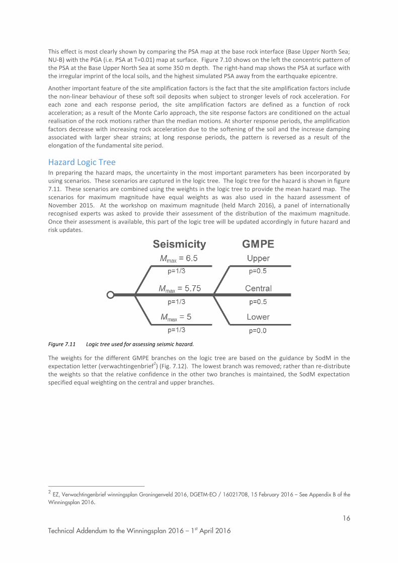
16
Technical Addendum to the Winningsplan 2016 – 1st April 2016
This effect is most clearly shown by comparing the PSA map at the base rock interface (Base Upper North Sea; NU-B) with the PGA (i.e. PSA at T=0.01) map at surface. Figure 7.10 shows on the left the concentric pattern of the PSA at the Base Upper North Sea at some 350 m depth. The right-hand map shows the PSA at surface with the irregular imprint of the local soils, and the highest simulated PSA away from the earthquake epicentre.
Another important feature of the site amplification factors is the fact that the site amplification factors include the non-linear behaviour of these soft soil deposits when subject to stronger levels of rock acceleration. For each zone and each response period, the site amplification factors are defined as a function of rock acceleration; as a result of the Monte Carlo approach, the site response factors are conditioned on the actual realisation of the rock motions rather than the median motions. At shorter response periods, the amplification factors decrease with increasing rock acceleration due to the softening of the soil and the increase damping associated with larger shear strains; at long response periods, the pattern is reversed as a result of the elongation of the fundamental site period.
Hazard Logic Tree In preparing the hazard maps, the uncertainty in the most important parameters has been incorporated by using scenarios. These scenarios are captured in the logic tree. The logic tree for the hazard is shown in figure 7.11. These scenarios are combined using the weights in the logic tree to provide the mean hazard map. The scenarios for maximum magnitude have equal weights as was also used in the hazard assessment of November 2015. At the workshop on maximum magnitude (held March 2016), a panel of internationally recognised experts was asked to provide their assessment of the distribution of the maximum magnitude. Once their assessment is available, this part of the logic tree will be updated accordingly in future hazard and risk updates.
Figure 7.11 Logic tree used for assessing seismic hazard.
The weights for the different GMPE branches on the logic tree are based on the guidance by SodM in the expectation letter (verwachtingenbrief
2) (Fig. 7.12). The lowest branch was removed; rather than re-distribute
the weights so that the relative confidence in the other two branches is maintained, the SodM expectation specified equal weighting on the central and upper branches.
2 EZ, Verwachtingenbrief winningsplan Groningenveld 2016, DGETM-EO / 16021708, 15 February 2016 – See Appendix B of the Winningsplan 2016.
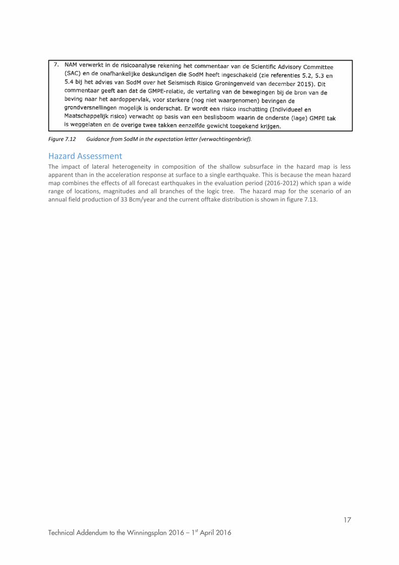
17
Technical Addendum to the Winningsplan 2016 – 1st April 2016
Figure 7.12 Guidance from SodM in the expectation letter (verwachtingenbrief).
Hazard Assessment The impact of lateral heterogeneity in composition of the shallow subsurface in the hazard map is less apparent than in the acceleration response at surface to a single earthquake. This is because the mean hazard map combines the effects of all forecast earthquakes in the evaluation period (2016-2012) which span a wide range of locations, magnitudes and all branches of the logic tree. The hazard map for the scenario of an annual field production of 33 Bcm/year and the current offtake distribution is shown in figure 7.13.

18
Technical Addendum to the Winningsplan 2016 – 1st April 2016
Max PGA = 0.21g
2016/1 – 2021/1 Figure 7.13 PGA hazard maps Period: 2016 – 2021, Production: 33 bcm/year, Compaction: Inversion, Activity Rate
Model: Version V2, 3.5≤M≤6.5, Metric: 0.2% year-1
chance of exceedance (10% chance in 50 years). Mean
hazard from logic tree.

19
Technical Addendum to the Winningsplan 2016 – 1st April 2016
a
b
c
d
e
f

20
Technical Addendum to the Winningsplan 2016 – 1st April 2016
Figure 8.14 Mean PGA hazard maps with an average 0.2% annual chance of exceedance (1 in 475 years) from 1/1/2016
to 1/1/2017 given the V2 linear compaction model and 6 production scenarios. Maximum values of the
mean PGA hazard are: (a) 0.206g, (b) 0.204g, (c) 0.200g, (d) 0.199g (e) 0.191g, (f) 0.194g.

21
Technical Addendum to the Winningsplan 2016 – 1st April 2016
a
b
c
d
e
f
Figure 7.15 As previous figure, except for the 5-year period 2016-2021. Maximum values of the mean PGA hazard are:
(a) 0.218g, (b) 0.215g, (c) 0.208g, (d) 0.207g (e) 0.197g, (f) 0.198g.
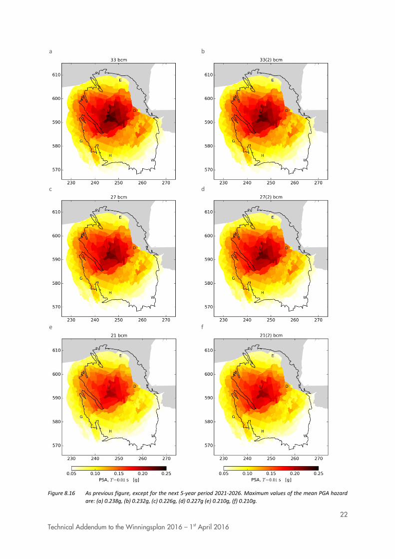
22
Technical Addendum to the Winningsplan 2016 – 1st April 2016
a
b
c
d
e
f
Figure 8.16 As previous figure, except for the next 5-year period 2021-2026. Maximum values of the mean PGA hazard
are: (a) 0.238g, (b) 0.232g, (c) 0.226g, (d) 0.227g (e) 0.210g, (f) 0.210g.

23
Technical Addendum to the Winningsplan 2016 – 1st April 2016
Disaggregation of Seismic Hazard The question which earthquakes have most impact on the hazard assessment was studied through a disaggregation of the hazard. Two disaggregations are shown; one for the hazard in the Loppersum area (Fig 7.17) and one for the city of Groningen (Fig. 7.18).
Figure 8.17 (a) Occurrence rates for peak spectral acceleration at 0.01 s as a function of magnitude, distance, and GMPE
epsilon, ε, for a single surface location directly above the region of maximum reservoir compaction. Grey
denotes no occurrence in any of the simulations. (b) The fractional contribution to the ground motion with a
0.2% annual probability of exceedance from January 2016 to January 2021.
The disaggregation of the hazard for the Loppersum area shows that the largest contribution to the hazard is from earthquakes within the Loppersum area (small distance of less than 5 km away with a magnitude ranging from 4 to 5). In contrast the largest contribution to the hazard in the Groningen city is from earthquakes with an epicenter approximately 10 km away from the city (towards the Loppersum area). To cause significant ground acceleration in the city of Groningen, these earthquakes located further away require a larger magnitude or GMPE epsilon to cause similar ground motions.
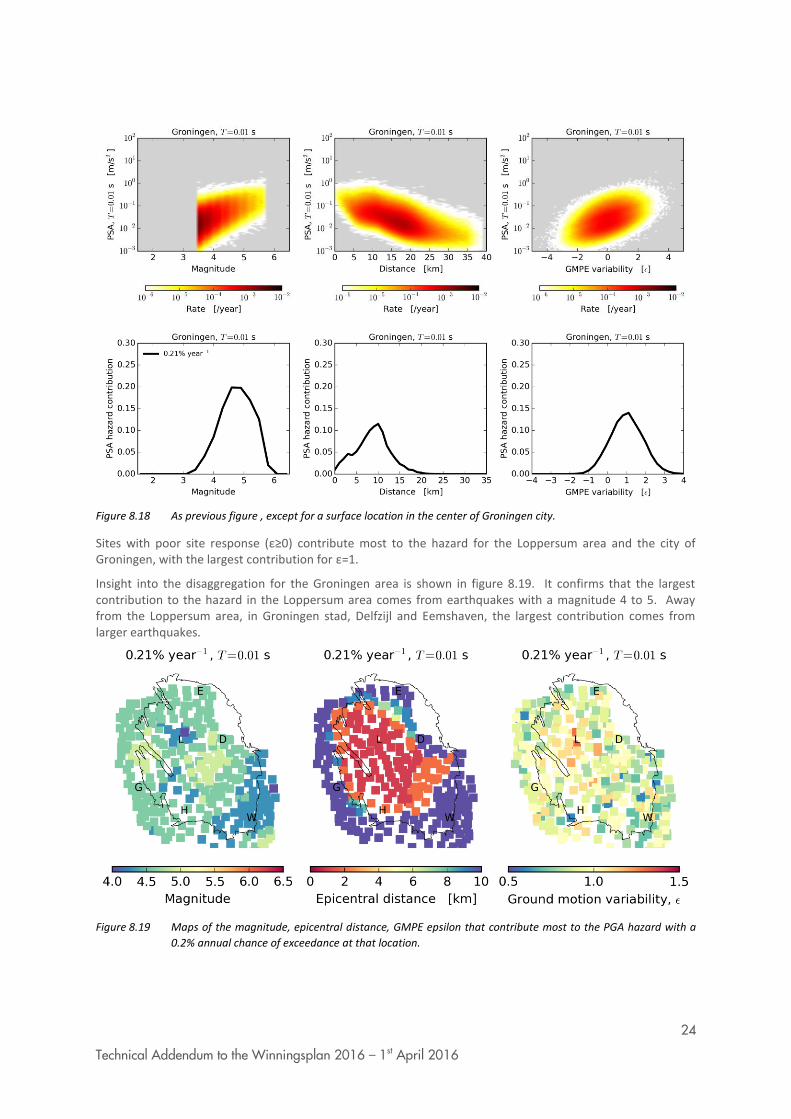
24
Technical Addendum to the Winningsplan 2016 – 1st April 2016
Figure 8.18 As previous figure , except for a surface location in the center of Groningen city.
Sites with poor site response (ε≥0) contribute most to the hazard for the Loppersum area and the city of Groningen, with the largest contribution for ε=1.
Insight into the disaggregation for the Groningen area is shown in figure 8.19. It confirms that the largest contribution to the hazard in the Loppersum area comes from earthquakes with a magnitude 4 to 5. Away from the Loppersum area, in Groningen stad, Delfzijl and Eemshaven, the largest contribution comes from larger earthquakes.
Figure 8.19 Maps of the magnitude, epicentral distance, GMPE epsilon that contribute most to the PGA hazard with a
0.2% annual chance of exceedance at that location.

25
Technical Addendum to the Winningsplan 2016 – 1st April 2016

1
Technical Addendum to the Winningsplan 2016 – 1st April 2016
Technical Addendum to the Winningsplan Groningen 2016 Production, Subsidence, Induced Earthquakes and Seismic Hazard and Risk Assessment in the Groningen Field PART IV Risk

2
Technical Addendum to the Winningsplan 2016 – 1st April 2016
The report “Technical Addendum to the Winningsplan Groningen 2016 - Production, Subsidence, Induced Earthquakes and Seismic Hazard and Risk Assessment in the Groningen Field” consists of five separate documents:
Document 1 Chapters 1 to 5; Summary and Production
Document 2 Chapter 6; Subsidence
Document 3 Chapter 7; Hazard
Document 4 Chapter 8; Risk
Document 5 Chapter 9; Damage and Appendices.
Each of these documents is also available as a *.pdf file of a size smaller than 10Mbyte, allowing sharing through e-mail.
© EP201603238413 Dit rapport is een weerslag van een voortdurend studie- en dataverzamelingsprogramma en bevat de stand der kennis van april 2016. Het copyright van dit rapport ligt bij de Nederlandse Aardolie Maatschappij B.V. Het copyright van de onderliggende studies berust bij de respectievelijke auteurs. Dit rapport of delen daaruit mogen alleen met een nadrukkelijke status-en bronvermelding worden overgenomen of gepubliceerd.
3
Technical Addendum to the Winningsplan 2016 – 1st April 2016
Contents 8 Risk Assessment .............................................................................................................................. 4
Probabilistic Risk Assessment ................................................................................................................. 4
Risk Metrics ......................................................................................................................................... 4
Inside Local Personal Risk 4
Object-bound Individual Risk 5
Number of People at Risk 5
Community Risk 5
Social Risk 5
Probabilistic Risk Assessment of Building Collapse ............................................................................ 7
Inside Local Personal Risk (ILPR) 7
Structural Upgrading Plan ................................................................................................................. 18
Impact of the Structural Upgrading Scenarios (Part 1) 18

4
Technical Addendum to the Winningsplan 2016 – 1st April 2016
8 Risk Assessment
Probabilistic Risk Assessment Risk Metrics The results from the probabilistic hazard and risk analysis (PHRA) are summarised via risk metrics which are related to the annualised probability of fatality for an individual person or for groups of people, taken as an average across the forecast period of the PHRA. These risk metrics - “Inside Local Personal Risk”, “Object-bound Individual Risk”, “Number of People at Risk”, “Community Risk, and “Social Risk” – are defined below. “Inside Local Personal Risk” and “Object-bound Individual Risk” are individual risk metrics (related to probability of fatality for an individual), whereas the remaining three metrics are measures of aggregate risk (related to probability of fatality for multiple people or for groups of people).
When measuring risk, it is important to select a risk metric that is appropriate given the purpose of the risk measurement. In many cases there is more than one option available as to which metric to use. An advisory committee, Commissie Meijdam, was established in early 2015 to advise on risk policy related to Groningen earthquakes, including the selection of risk metrics. In December 2015 the Commissie Meijdam shared its third and final advice with the Minister of Economic Affairs. The selection of risk metrics for this PHRA reflects the final advice published by Commissie Meijdam.
The following table contains a summary of the risk metrics used in this PHRA along with the purpose of the risk metric:
Type of Metric Risk Metric Purpose(s)
Individual
Inside Local Personal Risk* (ILPR)
1. Individual risk metrics to measure building collapse risk (ILPR) and falling object risk (OIR) relative to norm of 10
-5 overall individual risk
2. Check if any buildings/objects have individual Risk above 10
-4 (high priority for action)
Object-bound Individual Risk* (OIR)
Aggregate
Number of people (or buildings/objects) at risk
Assess overall scale of risk across region and therefore determine do-ability of structural upgrading program
Community Risk Input towards prioritisation of buildings/objects (which don't comply with individual risk norm) within structural upgrading program
Social Risk*
1. Provide risk insights to National Coordinator Groningen for prioritisation of communities in multi-year plan
2. Consider additional measures (where “reasonable”) beyond reducing individual risk to below 10
-5
*For clarity, Dutch translations of these metrics in the final Commissie Meijdam advice are:
Local Personal Risk = “Plaatsgebonden Risico”
Object-bound Individual Risk = “Objectgebonden Individueel Aardbevingsrisico”
Social Risk = “Maatschappelijk Risico”
Inside Local Personal Risk “Local Personal Risk” (LPR) is generally defined as the annual probability of fatality for a fictional person, who is continuously present without protection at a specific at-risk location. For Groningen earthquakes, LPR is defined as follows: “the probability of death of a fictional person who is permanently in or near a building”. “Inside LPR” (ILPR) focuses on the risk to people inside of buildings, and assumes that the fictional person is present inside the building 100% of the time, and the location of the person is uniformly and randomly distributed inside the building i.e. if 10% of the building collapses there is a 10% probability that the fictional person will be in the collapsed part of the building. In this PHRA, ILPR is used to measure the fatality risk to people inside the building from building collapse. The mean value of the ILPR is the primary metric used to

5
Technical Addendum to the Winningsplan 2016 – 1st April 2016
compare against the 10-5
individual risk norm (as recommended by Commissie Meijdam and accepted by the Ministry of Economic Affairs, requires the fatality risk for a person inside a building to be less than 10
-5 per
year).
Whereas ILPR is normally calculated for a specific building, it can also be averaged across a number of buildings within a geographical area, such as within a map grid cell. In this report, the averaging of ILPR uses weighting based on the estimated day/night population of each building.
Object-bound Individual Risk The Dutch term for Object-bound individual risk (OIR) is “Objectgebonden Individueel Aardbevingsrisico” OIA. Object-bound individual risk (OIR) is used to measure the contribution to individual risk from non-structural elements of buildings, such as chimneys, parapets and gables, which pose a potential falling object risk to people inside and outside of buildings. The assessment of falling object risk is described in a separate report, however the key metric used to measure falling object risk, OIR, is defined here for completeness. In this context, OIR is defined as the annual probability of fatality for a “representative person” from a specified potential falling object. OIR takes into account the proportion of time that a “representative person” is exposed to the potential falling object risk, unlike LPR which assumes a person is exposed to the risk 100% of the time. Specifically, OIR is equal to LPR multiplied by the percentage exposure time for the “representative person”. The calculation of OIR therefore requires exposure time assumptions to be made for a “representative person” – the final Commissie Meijdam advice (Appendix 2 of this advice) provides an example of how to do this, and the specific assumptions used for the measurement of falling object risk are described in the appendices of the falling object risk assessment report.
The OIR acceptance threshold for falling objects has not yet been defined (in the final Commissie Miejdam advice, or otherwise), since the OIR for a falling object is only one contribution towards overall individual risk, and the norm is based on overall individual risk of 10
-5 taking into account all earthquake related risks. In the
meantime (until an OIR acceptance threshold is defined), it is assumed for prioritization purposes that if the OIR for a falling object is significantly (e.g. an order of magnitude or more) less than 10
-5 then the object is very
likely to comply with the individual risk norm.
Number of People at Risk The number of people at risk is used in this PHRA to determine the overall scale of the risk from Groningen earthquakes, which helps to assess the feasibility of (and options for) the measures available for mitigating the risk to comply with the defined norms (i.e. to reduce risk to acceptable level in an acceptable timeframe). For example, for a given production scenario the feasibility of the structural upgrading program can be assessed. In this PHRA, the number of people at risk is shown for ILPR, and is presented as a cumulative distribution (of people versus risk level). An ILPR distribution is also presented based on the number of buildings (rather than people), which can be easily compared to the structural upgrading scope.
Community Risk Community Risk (CR) is the annualised rate of fatalities for a specified risk, with units of fatalities per year. CR is calculated by multiplying the LPR for a specified risk by the average number of people present in the at-risk area. Inside a building, the at-risk area is defined as the entire area inside the building, and CR is calculated by multiplying LPR by average number of building occupants (taking into account the proportion of time that the building is occupied). Outside of buildings, the at-risk area is defined as the area up to 5m from the building façade (based on empirical evidence of masonry falling from buildings), and CR is calculated by multiplying the LPR for this at-risk area by the average number of people in the at-risk area. The method for calculating CR for the area outside of buildings is further described in the falling objects risk assessment report.
CR is used as an input towards the prioritisation of buildings or objects that don’t meet the individual risk norm for upgrading in the structural upgrading program.
Social Risk A new risk metric, Social Risk (“Maatschappelijk Veiligheidsrisico” in Dutch) was introduced for the first time in the final Commissie Meijdam advice as an alternative to Group Risk. Social Risk is an assessment of the frequency (f) with which defined numbers of fatalities (N) occur due to earthquakes, with an offset for “basic

6
Technical Addendum to the Winningsplan 2016 – 1st April 2016
safety” (assuming everyone exposed to the earthquake risk is at uncorrelated 10-5
individual risk). The calculation procedure for Social Risk is fully described in the final Commissie Meijdam advice, appendix 2.
Social Risk is calculated for several “communities” (centres of population such as villages, towns or cities), where the “communities” have been defined by the Ministry of Economic Affairs in consultation with the National Coordinator Groningen.
There are two main purposes of Social Risk:
1. To assist the National Coordinator Groningen with the prioritisation of “communities” in the multi-year plan by highlighting communities with higher Social Risk (in relative terms).
2. To assist the assessment of certain risks like the risk of falling objects in a busy shopping street, taking into account the reasonable investments needed to reduce the risks.
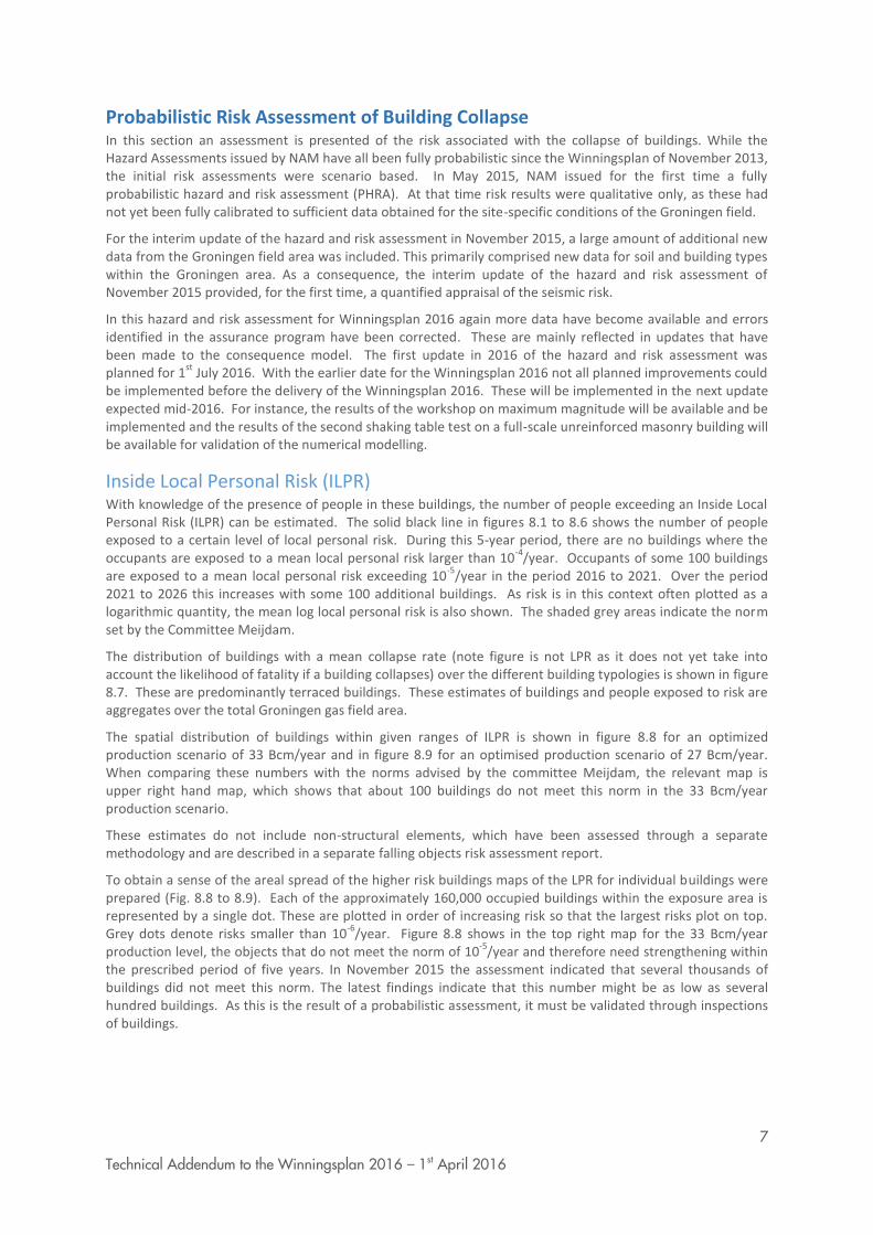
7
Technical Addendum to the Winningsplan 2016 – 1st April 2016
Probabilistic Risk Assessment of Building Collapse In this section an assessment is presented of the risk associated with the collapse of buildings. While the Hazard Assessments issued by NAM have all been fully probabilistic since the Winningsplan of November 2013, the initial risk assessments were scenario based. In May 2015, NAM issued for the first time a fully probabilistic hazard and risk assessment (PHRA). At that time risk results were qualitative only, as these had not yet been fully calibrated to sufficient data obtained for the site-specific conditions of the Groningen field.
For the interim update of the hazard and risk assessment in November 2015, a large amount of additional new data from the Groningen field area was included. This primarily comprised new data for soil and building types within the Groningen area. As a consequence, the interim update of the hazard and risk assessment of November 2015 provided, for the first time, a quantified appraisal of the seismic risk.
In this hazard and risk assessment for Winningsplan 2016 again more data have become available and errors identified in the assurance program have been corrected. These are mainly reflected in updates that have been made to the consequence model. The first update in 2016 of the hazard and risk assessment was planned for 1
st July 2016. With the earlier date for the Winningsplan 2016 not all planned improvements could
be implemented before the delivery of the Winningsplan 2016. These will be implemented in the next update expected mid-2016. For instance, the results of the workshop on maximum magnitude will be available and be implemented and the results of the second shaking table test on a full-scale unreinforced masonry building will be available for validation of the numerical modelling.
Inside Local Personal Risk (ILPR) With knowledge of the presence of people in these buildings, the number of people exceeding an Inside Local Personal Risk (ILPR) can be estimated. The solid black line in figures 8.1 to 8.6 shows the number of people exposed to a certain level of local personal risk. During this 5-year period, there are no buildings where the occupants are exposed to a mean local personal risk larger than 10
-4/year. Occupants of some 100 buildings
are exposed to a mean local personal risk exceeding 10-5
/year in the period 2016 to 2021. Over the period 2021 to 2026 this increases with some 100 additional buildings. As risk is in this context often plotted as a logarithmic quantity, the mean log local personal risk is also shown. The shaded grey areas indicate the norm set by the Committee Meijdam.
The distribution of buildings with a mean collapse rate (note figure is not LPR as it does not yet take into account the likelihood of fatality if a building collapses) over the different building typologies is shown in figure 8.7. These are predominantly terraced buildings. These estimates of buildings and people exposed to risk are aggregates over the total Groningen gas field area.
The spatial distribution of buildings within given ranges of ILPR is shown in figure 8.8 for an optimized production scenario of 33 Bcm/year and in figure 8.9 for an optimised production scenario of 27 Bcm/year. When comparing these numbers with the norms advised by the committee Meijdam, the relevant map is upper right hand map, which shows that about 100 buildings do not meet this norm in the 33 Bcm/year production scenario.
These estimates do not include non-structural elements, which have been assessed through a separate methodology and are described in a separate falling objects risk assessment report.
To obtain a sense of the areal spread of the higher risk buildings maps of the LPR for individual buildings were prepared (Fig. 8.8 to 8.9). Each of the approximately 160,000 occupied buildings within the exposure area is represented by a single dot. These are plotted in order of increasing risk so that the largest risks plot on top. Grey dots denote risks smaller than 10
-6/year. Figure 8.8 shows in the top right map for the 33 Bcm/year
production level, the objects that do not meet the norm of 10-5
/year and therefore need strengthening within the prescribed period of five years. In November 2015 the assessment indicated that several thousands of buildings did not meet this norm. The latest findings indicate that this number might be as low as several hundred buildings. As this is the result of a probabilistic assessment, it must be validated through inspections of buildings.

8
Technical Addendum to the Winningsplan 2016 – 1st April 2016
Figure 8.1 Number of buildings and people exceeding a given inside local personal risk shown on (a) a linear scale and
(b) a log scale for the 33 bcm production scenario and the 2016-2021 assessment period. The grey areas
indicate the norm advised by the Committee Meijdam.
Figure 8.2 As Figure 8.1, except for just the mean inside local personal risk. Light grey band indicates LPR range
between 10-4
/year and 10-5
/year. Buildings in this range need to be structurally upgraded within 5 years.
Dark grey indicated LPR>10-4
/year.
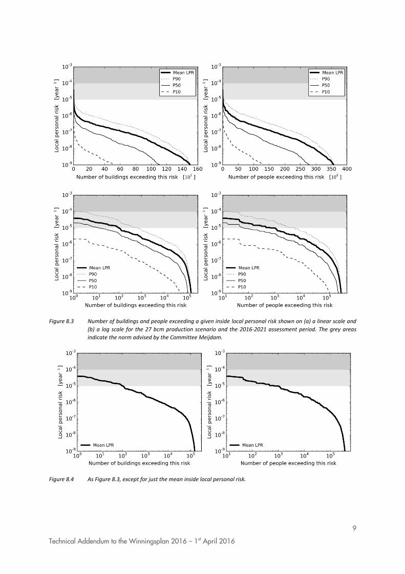
9
Technical Addendum to the Winningsplan 2016 – 1st April 2016
Figure 8.3 Number of buildings and people exceeding a given inside local personal risk shown on (a) a linear scale and
(b) a log scale for the 27 bcm production scenario and the 2016-2021 assessment period. The grey areas
indicate the norm advised by the Committee Meijdam.
Figure 8.4 As Figure 8.3, except for just the mean inside local personal risk.
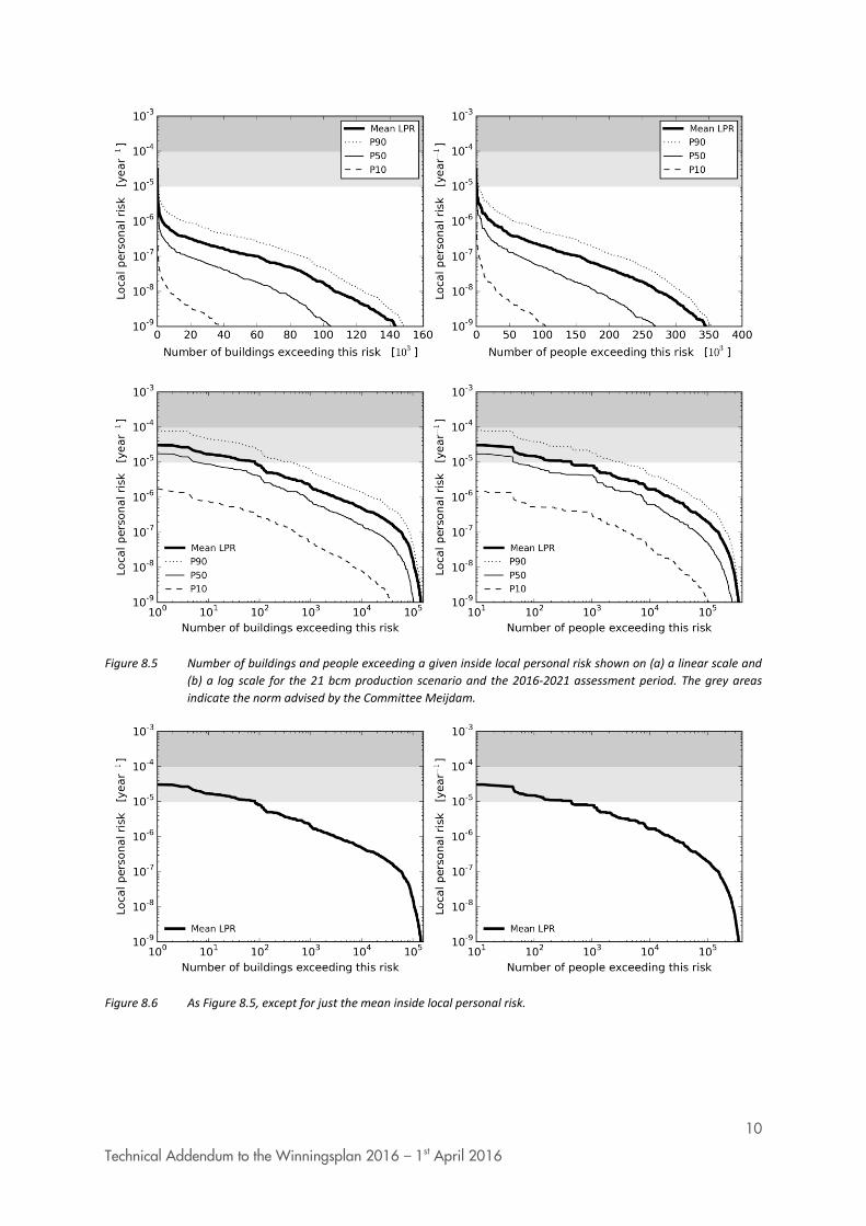
10
Technical Addendum to the Winningsplan 2016 – 1st April 2016
Figure 8.5 Number of buildings and people exceeding a given inside local personal risk shown on (a) a linear scale and
(b) a log scale for the 21 bcm production scenario and the 2016-2021 assessment period. The grey areas
indicate the norm advised by the Committee Meijdam.
Figure 8.6 As Figure 8.5, except for just the mean inside local personal risk.

11
Technical Addendum to the Winningsplan 2016 – 1st April 2016
These estimates of buildings and people exposed to risk are aggregates over the total Groningen gas field area.
Figure 8.7 Numbers of buildings exceeding a given average annual collapse rate for the 2016-2021 assessment period,
the 33 bcm production scenario (top row) and the base-case of the logic tree. Exceedance curves are shown
according to (left) building material, (right) building typology. The named building topologies denote the
top-ten ranked according to the number of buildings with a collapse rate of at least 10-5
/year.
Second row as top row, but for 27 bcm production scenario.
Bottom row as top row, but for 21 bcm production scenario.

12
Technical Addendum to the Winningsplan 2016 – 1st April 2016
10-4<ILPR<10-3
(buildings 0)
10-5<ILPR<10-4
(buildings c. 100)
10-6<ILPR<10-5
(buildings c. 6,000)
10-7<ILPR<10-6
(buildings c. 65,000)
Figure 8.8 Inside local personal risk, LPR for every individual building within four equal risk bands from 10-7
to
10-3
/year for the 5-year assessment period 2016 to 2021 under the 33 bcm production scenario.
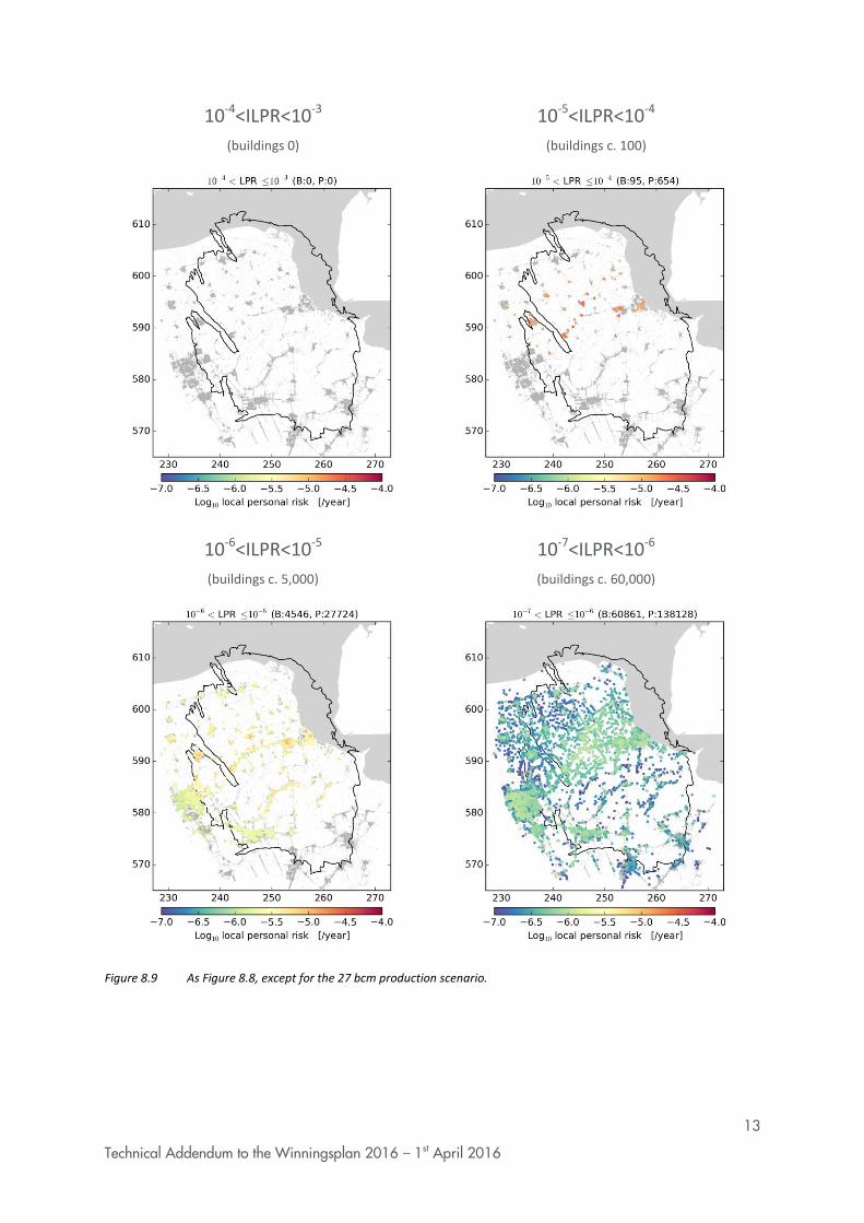
13
Technical Addendum to the Winningsplan 2016 – 1st April 2016
10-4<ILPR<10-3
(buildings 0)
10-5<ILPR<10-4
(buildings c. 100)
10-6<ILPR<10-5
(buildings c. 5,000)
10-7<ILPR<10-6
(buildings c. 60,000)
Figure 8.9 As Figure 8.8, except for the 27 bcm production scenario.

14
Technical Addendum to the Winningsplan 2016 – 1st April 2016
The spatial distribution of buildings within given ranges of ILPR is shown in figure 8.6 for a production scenario of 33 Bcm/year and in figure 8.7 for a production scenario of 27 Bcm/year. When comparing these numbers with the norms advised by the committee Meijdam, the relevant map is upper right hand map.
Disaggregation of Inside Local Personal Risk (ILPR)
A disaggregation of contributions to the base-case ILPR was performed for magnitude, distance from the
epicentre, the ground motion variability measure , and spectral acceleration causing building collapse. Figure 8.10 shows the results for the residential apartment buildings of unreinforced masonry with silica-calcium load bearing walls (type B) in the Loppersum area (typology RESA-URM-B).
Figure 8.10 The fractional contribution to ILPR for the RESA-URM-B building typology at two locations: Loppersum (top
row) and Groningen city centre (bottom row). This result was obtained for the 2016 to 2021 assessment
period under the 33 bcm/year production scenario and the base-case scenario of the risk logic tree.
Fluctuations between neighbouring points are due to finite sampling effects of the Monte Carlo procedure;
nonetheless the underlying trends are clear.
As for hazard, earthquakes in the Loppersum area (i.e. at epicentral distances less than 5 km) contribute most to the risk for this area. For Groningen city, earthquakes at an epicentral distance of 10 km (i.e. in the Loppersum area) are the most important contribution to the risk.

15
Technical Addendum to the Winningsplan 2016 – 1st April 2016
Figure 8.11 Risk disaggregation maps for the RESA-URM-B building typology showing the modal contribution to ILPR at
each map location for the period 2016 to 2021 under the 33 bcm/year production scenario and the base-
case logic tree scenario.
The areal representation of the risk disaggregation is shown in figure 8.11. For areas with low risk (like the South East of the field) the risk disaggregation in this figure is less reliable due to finite sampling effects of the Monte Carlo process for these especially small values of ILPR.
Figure 8.12 Same as figure 8.10 for the RECA-RC-A-L4S building typology
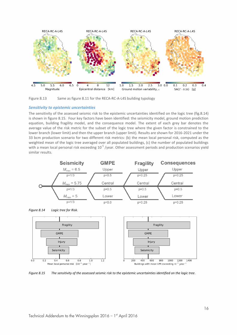
16
Technical Addendum to the Winningsplan 2016 – 1st April 2016
Figure 8.13 Same as figure 8.11 for the RECA-RC-A-L4S building typology
Sensitivity to epistemic uncertainties
The sensitivity of the assessed seismic risk to the epistemic uncertainties identified on the logic tree (fig.8.14) is shown in figure 8.15. Four key factors have been identified: the seismicity model, ground motion prediction equation, building fragility model, and the consequence model. The extent of each grey bar denotes the average value of the risk metric for the subset of the logic tree where the given factor is constrained to the lower branch (lower limit) and then the upper branch (upper limit). Results are shown for 2016-2021 under the 33 bcm production scenario for two different risk metrics: (b) the mean local personal risk, computed as the weighted mean of the logic tree averaged over all populated buildings, (c) the number of populated buildings with a mean local personal risk exceeding 10
-5 /year. Other assessment periods and production scenarios yield
similar results.
Figure 8.14 Logic tree for Risk.
Figure 8.15 The sensitivity of the assessed seismic risk to the epistemic uncertainties identified on the logic tree.
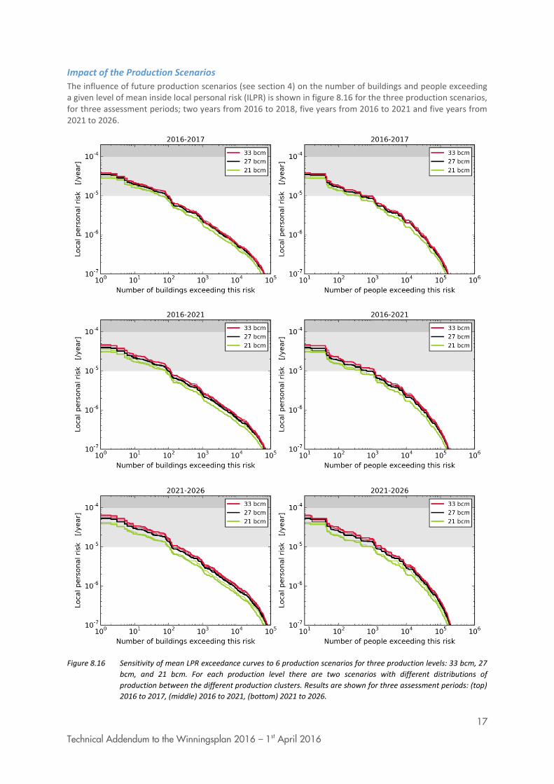
17
Technical Addendum to the Winningsplan 2016 – 1st April 2016
Impact of the Production Scenarios
The influence of future production scenarios (see section 4) on the number of buildings and people exceeding a given level of mean inside local personal risk (ILPR) is shown in figure 8.16 for the three production scenarios, for three assessment periods; two years from 2016 to 2018, five years from 2016 to 2021 and five years from 2021 to 2026.
Figure 8.16 Sensitivity of mean LPR exceedance curves to 6 production scenarios for three production levels: 33 bcm, 27
bcm, and 21 bcm. For each production level there are two scenarios with different distributions of
production between the different production clusters. Results are shown for three assessment periods: (top)
2016 to 2017, (middle) 2016 to 2021, (bottom) 2021 to 2026.
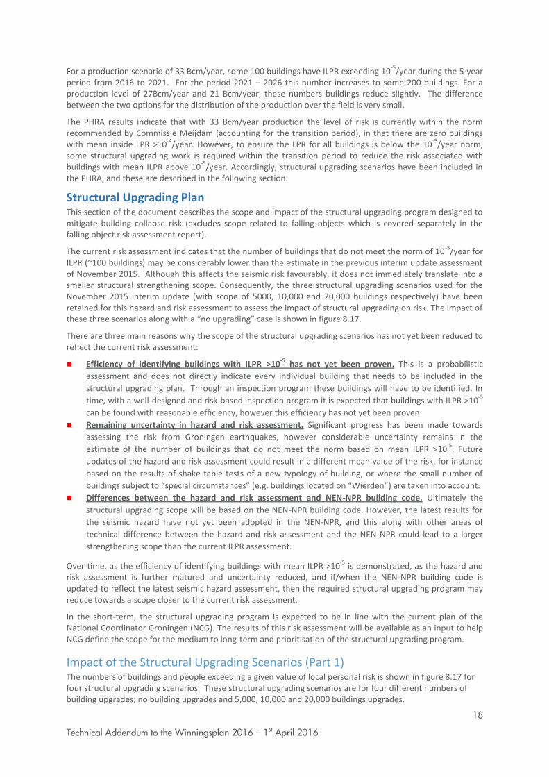
18
Technical Addendum to the Winningsplan 2016 – 1st April 2016
For a production scenario of 33 Bcm/year, some 100 buildings have ILPR exceeding 10-5
/year during the 5-year period from 2016 to 2021. For the period 2021 – 2026 this number increases to some 200 buildings. For a production level of 27Bcm/year and 21 Bcm/year, these numbers buildings reduce slightly. The difference between the two options for the distribution of the production over the field is very small.
The PHRA results indicate that with 33 Bcm/year production the level of risk is currently within the norm recommended by Commissie Meijdam (accounting for the transition period), in that there are zero buildings with mean inside LPR >10
-4/year. However, to ensure the LPR for all buildings is below the 10
-5/year norm,
some structural upgrading work is required within the transition period to reduce the risk associated with buildings with mean ILPR above 10
-5/year. Accordingly, structural upgrading scenarios have been included in
the PHRA, and these are described in the following section.
Structural Upgrading Plan This section of the document describes the scope and impact of the structural upgrading program designed to mitigate building collapse risk (excludes scope related to falling objects which is covered separately in the falling object risk assessment report).
The current risk assessment indicates that the number of buildings that do not meet the norm of 10-5
/year for ILPR (~100 buildings) may be considerably lower than the estimate in the previous interim update assessment of November 2015. Although this affects the seismic risk favourably, it does not immediately translate into a smaller structural strengthening scope. Consequently, the three structural upgrading scenarios used for the November 2015 interim update (with scope of 5000, 10,000 and 20,000 buildings respectively) have been retained for this hazard and risk assessment to assess the impact of structural upgrading on risk. The impact of these three scenarios along with a “no upgrading” case is shown in figure 8.17.
There are three main reasons why the scope of the structural upgrading scenarios has not yet been reduced to reflect the current risk assessment:
Efficiency of identifying buildings with ILPR >10-5
has not yet been proven. This is a probabilistic
assessment and does not directly indicate every individual building that needs to be included in the
structural upgrading plan. Through an inspection program these buildings will have to be identified. In
time, with a well-designed and risk-based inspection program it is expected that buildings with ILPR >10-5
can be found with reasonable efficiency, however this efficiency has not yet been proven.
Remaining uncertainty in hazard and risk assessment. Significant progress has been made towards
assessing the risk from Groningen earthquakes, however considerable uncertainty remains in the
estimate of the number of buildings that do not meet the norm based on mean ILPR >10-5
. Future
updates of the hazard and risk assessment could result in a different mean value of the risk, for instance
based on the results of shake table tests of a new typology of building, or where the small number of
buildings subject to “special circumstances” (e.g. buildings located on “Wierden”) are taken into account.
Differences between the hazard and risk assessment and NEN-NPR building code. Ultimately the
structural upgrading scope will be based on the NEN-NPR building code. However, the latest results for
the seismic hazard have not yet been adopted in the NEN-NPR, and this along with other areas of
technical difference between the hazard and risk assessment and the NEN-NPR could lead to a larger
strengthening scope than the current ILPR assessment.
Over time, as the efficiency of identifying buildings with mean ILPR >10-5
is demonstrated, as the hazard and risk assessment is further matured and uncertainty reduced, and if/when the NEN-NPR building code is updated to reflect the latest seismic hazard assessment, then the required structural upgrading program may reduce towards a scope closer to the current risk assessment.
In the short-term, the structural upgrading program is expected to be in line with the current plan of the National Coordinator Groningen (NCG). The results of this risk assessment will be available as an input to help NCG define the scope for the medium to long-term and prioritisation of the structural upgrading program.
Impact of the Structural Upgrading Scenarios (Part 1) The numbers of buildings and people exceeding a given value of local personal risk is shown in figure 8.17 for four structural upgrading scenarios. These structural upgrading scenarios are for four different numbers of building upgrades; no building upgrades and 5,000, 10,000 and 20,000 buildings upgrades.
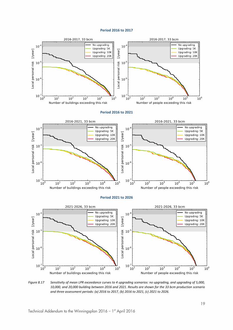
19
Technical Addendum to the Winningsplan 2016 – 1st April 2016
Period 2016 to 2017
Period 2016 to 2021
Period 2021 to 2026
Figure 8.17 Sensitivity of mean LPR exceedance curves to 4 upgrading scenarios: no upgrading, and upgrading of 5,000,
10,000, and 20,000 building between 2016 and 2021. Results are shown for the 33 bcm production scenario
and three assessment periods: (a) 2016 to 2017, (b) 2016 to 2021, (c) 2021 to 2026.

20
Technical Addendum to the Winningsplan 2016 – 1st April 2016
For the production scenario of 33 Bcm/year each of the structural upgrading scenarios achieves a reduction of the ILPR to below the 10
-5 /year norm (fig. 8.17 and 8.19). This also holds for the 27 bcm/year production
scenario (fig. 8.18).
21
Technical Addendum to the Winningsplan 2016 – 1st April 2016
Period 2016 to 2017
Period 2016 to 2021
Period 2021 to 2026
Figure 8.18 As figure 8.17, except for the 27 bcm production scenario.

22
Technical Addendum to the Winningsplan 2016 – 1st April 2016
a
b
c
Figure 8.19 As Figure 8.17, except for the results are shown on linear scales for local personal risk exceeding 10
-5/year

23
Technical Addendum to the Winningsplan 2016 – 1st April 2016
1
Technical Addendum to the Winningsplan 2016 – 1st April 2016
Technical Addendum to the Winningsplan Groningen 2016 Production, Subsidence, Induced Earthquakes and Seismic Hazard and Risk Assessment in the Groningen Field PART V Damage and Appendices

2
Technical Addendum to the Winningsplan 2016 – 1st April 2016
The report “Technical Addendum to the Winningsplan Groningen 2016 - Production, Subsidence, Induced Earthquakes and Seismic Hazard and Risk Assessment in the Groningen Field” consists of five separate documents:
Document 1 Chapters 1 to 5; Summary and Production
Document 2 Chapter 6; Subsidence
Document 3 Chapter 7; Hazard
Document 4 Chapter 8; Risk
Document 5 Chapter 9; Damage and Appendices.
Each of these documents is also available as a *.pdf file of a size smaller than 10Mbyte, allowing sharing through e-mail.
© EP201603238413 Dit rapport is een weerslag van een voortdurend studie- en dataverzamelingsprogramma en bevat de stand der kennis van april 2016. Het copyright van dit rapport ligt bij de Nederlandse Aardolie Maatschappij B.V. Het copyright van de onderliggende studies berust bij de respectievelijke auteurs. Dit rapport of delen daaruit mogen alleen met een nadrukkelijke status-en bronvermelding worden overgenomen of gepubliceerd.

3
Technical Addendum to the Winningsplan 2016 – 1st April 2016
Contents 9 Building Damage ............................................................................................................................. 4
Introduction ........................................................................................................................................ 4
SBR Guideline Part A ........................................................................................................................... 4
Analysis of Historical Damage Claims ................................................................................................. 5
Comparison Damage Claims after Huizinge 2012 and Hellum 2015 .................................................. 6
Temporal Comparison 7
Spatial Comparison 8
Predicting chance of Building Damage; Kalibratiestudie schade door aardbevingen ........................ 8
Damage Huizinge Earthquake 11
Damage Hellum Earthquake 12
A growing trend toward C-damage ................................................................................................... 13
TNO building sensors register earthquakes and more ..................................................................... 16
Conclusions ....................................................................................................................................... 19
Appendix A - Spectral Hazard Maps ...................................................................................................... 20
Appendix B - Seismic Event Rate and .................................................................................................... 23
Annual Total Seismic Moment (2016 – 2035) ....................................................................................... 23
Appendix C – Hazard Maps Large Format ............................................................................................. 25
References ............................................................................................................................................ 28
List of abbreviations .............................................................................................................................. 28
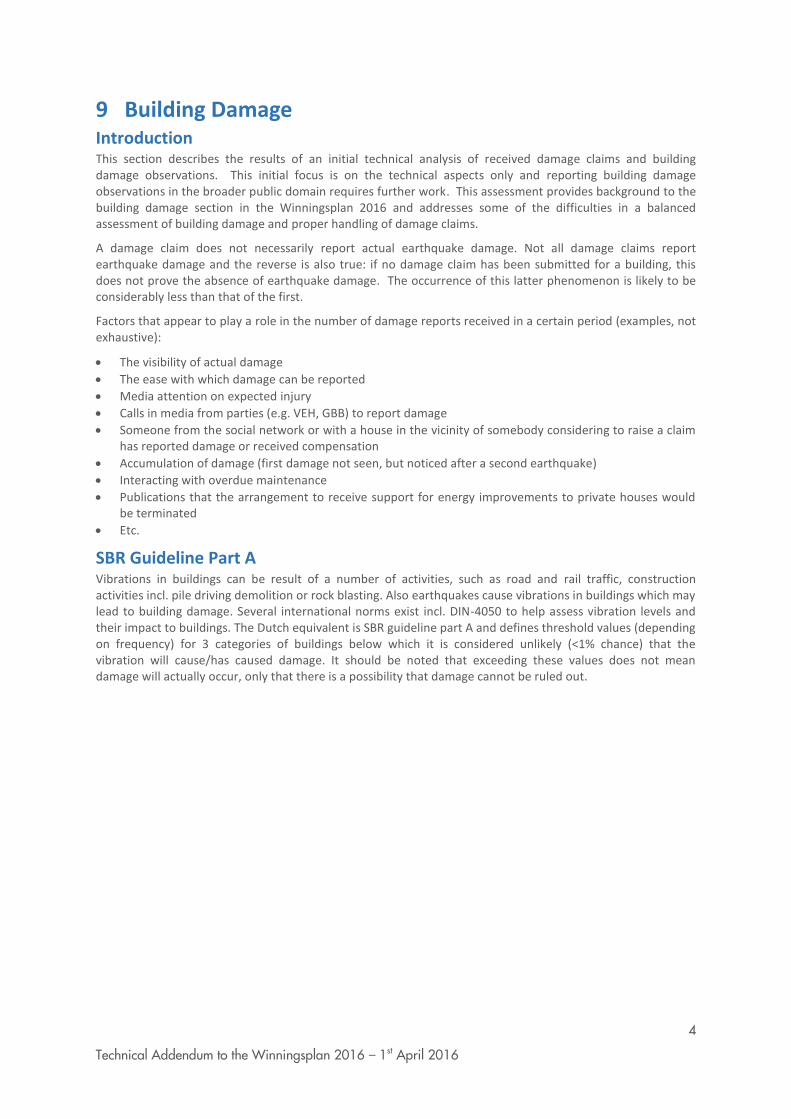
4
Technical Addendum to the Winningsplan 2016 – 1st April 2016
9 Building Damage Introduction This section describes the results of an initial technical analysis of received damage claims and building damage observations. This initial focus is on the technical aspects only and reporting building damage observations in the broader public domain requires further work. This assessment provides background to the building damage section in the Winningsplan 2016 and addresses some of the difficulties in a balanced assessment of building damage and proper handling of damage claims.
A damage claim does not necessarily report actual earthquake damage. Not all damage claims report earthquake damage and the reverse is also true: if no damage claim has been submitted for a building, this does not prove the absence of earthquake damage. The occurrence of this latter phenomenon is likely to be considerably less than that of the first.
Factors that appear to play a role in the number of damage reports received in a certain period (examples, not exhaustive):
The visibility of actual damage
The ease with which damage can be reported
Media attention on expected injury
Calls in media from parties (e.g. VEH, GBB) to report damage
Someone from the social network or with a house in the vicinity of somebody considering to raise a claim has reported damage or received compensation
Accumulation of damage (first damage not seen, but noticed after a second earthquake)
Interacting with overdue maintenance
Publications that the arrangement to receive support for energy improvements to private houses would be terminated
Etc.
SBR Guideline Part A Vibrations in buildings can be result of a number of activities, such as road and rail traffic, construction activities incl. pile driving demolition or rock blasting. Also earthquakes cause vibrations in buildings which may lead to building damage. Several international norms exist incl. DIN-4050 to help assess vibration levels and their impact to buildings. The Dutch equivalent is SBR guideline part A and defines threshold values (depending on frequency) for 3 categories of buildings below which it is considered unlikely (<1% chance) that the vibration will cause/has caused damage. It should be noted that exceeding these values does not mean damage will actually occur, only that there is a possibility that damage cannot be ruled out.
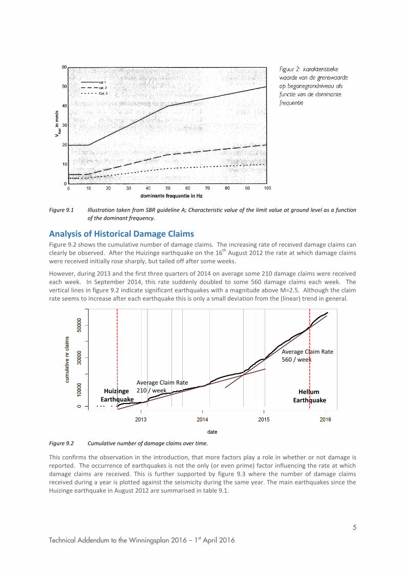
5
Technical Addendum to the Winningsplan 2016 – 1st April 2016
Figure 9.1 Illustration taken from SBR guideline A; Characteristic value of the limit value at ground level as a function
of the dominant frequency.
Analysis of Historical Damage Claims Figure 9.2 shows the cumulative number of damage claims. The increasing rate of received damage claims can clearly be observed. After the Huizinge earthquake on the 16
th August 2012 the rate at which damage claims
were received initially rose sharply, but tailed off after some weeks.
However, during 2013 and the first three quarters of 2014 on average some 210 damage claims were received each week. In September 2014, this rate suddenly doubled to some 560 damage claims each week. The vertical lines in figure 9.2 indicate significant earthquakes with a magnitude above M=2.5. Although the claim rate seems to increase after each earthquake this is only a small deviation from the (linear) trend in general.
Figure 9.2 Cumulative number of damage claims over time.
This confirms the observation in the introduction, that more factors play a role in whether or not damage is reported. The occurrence of earthquakes is not the only (or even prime) factor influencing the rate at which damage claims are received. This is further supported by figure 9.3 where the number of damage claims received during a year is plotted against the seismicity during the same year. The main earthquakes since the Huizinge earthquake in August 2012 are summarised in table 9.1.
Average Claim Rate210 / week
Average Claim Rate560 / week
HuizingeEarthquake
HellumEarthquake
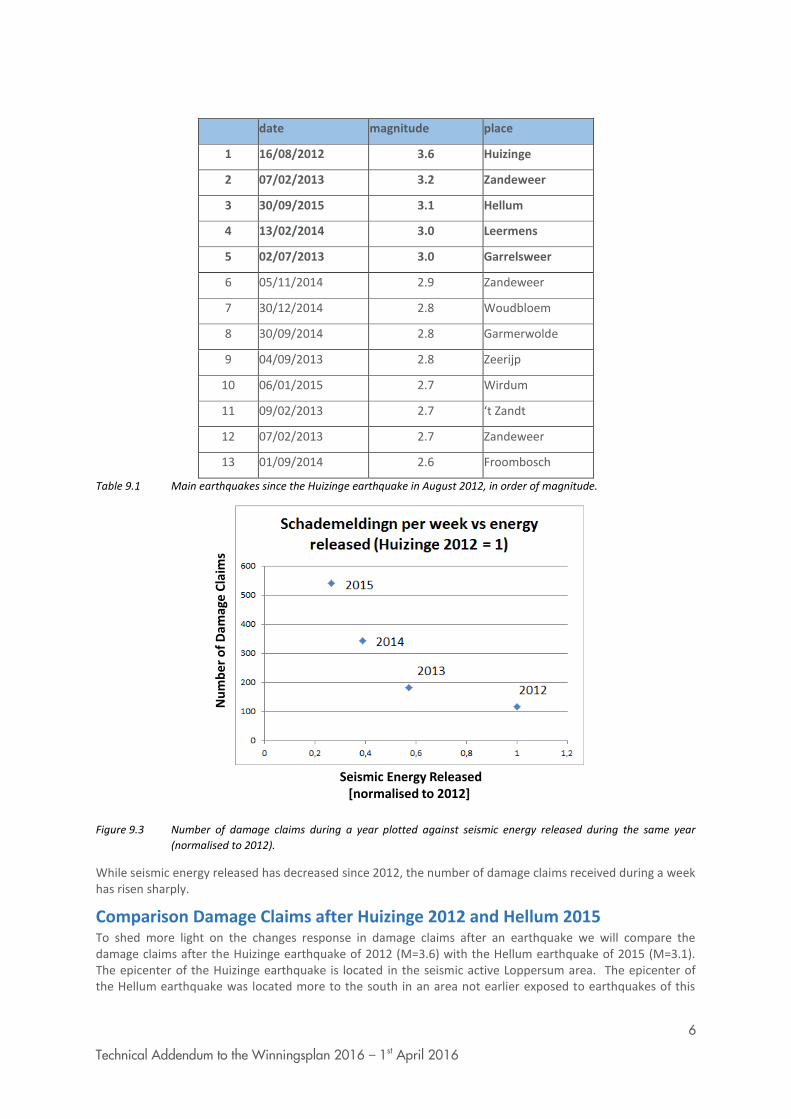
6
Technical Addendum to the Winningsplan 2016 – 1st April 2016
date magnitude place
1 16/08/2012 3.6 Huizinge
2 07/02/2013 3.2 Zandeweer
3 30/09/2015 3.1 Hellum
4 13/02/2014 3.0 Leermens
5 02/07/2013 3.0 Garrelsweer
6 05/11/2014 2.9 Zandeweer
7 30/12/2014 2.8 Woudbloem
8 30/09/2014 2.8 Garmerwolde
9 04/09/2013 2.8 Zeerijp
10 06/01/2015 2.7 Wirdum
11 09/02/2013 2.7 ‘t Zandt
12 07/02/2013 2.7 Zandeweer
13 01/09/2014 2.6 Froombosch
Table 9.1 Main earthquakes since the Huizinge earthquake in August 2012, in order of magnitude.
Figure 9.3 Number of damage claims during a year plotted against seismic energy released during the same year
(normalised to 2012).
While seismic energy released has decreased since 2012, the number of damage claims received during a week has risen sharply.
Comparison Damage Claims after Huizinge 2012 and Hellum 2015 To shed more light on the changes response in damage claims after an earthquake we will compare the damage claims after the Huizinge earthquake of 2012 (M=3.6) with the Hellum earthquake of 2015 (M=3.1). The epicenter of the Huizinge earthquake is located in the seismic active Loppersum area. The epicenter of the Hellum earthquake was located more to the south in an area not earlier exposed to earthquakes of this
Seismic Energy Released[normalised to 2012]
Nu
mb
er
of
Dam
age
Cla
ims

7
Technical Addendum to the Winningsplan 2016 – 1st April 2016
magnitude. Prior to the Hellum earthquake no significant earthquake with magnitude above M=2 had occurred for 9 months. This made the Hellum earthquake a both laterally and temporally an isolated event.
Temporal Comparison The rate at which the claims are received after the earthquake is analysed first . The number of damage claims received in the weeks following these two earthquake events is very different (fig. 9.4).
Figure 9.4 Number of damage claims during a week compared for the Huizinge (blue) and Hellum (red) earthquakes.
After the Huizinge earthquake claims received rose sharply only to subside three weeks later (fig. 9.5). The maximum number of claims received was some 600 claims in the second week. After two month the number of claims received each week has declined below 40.
Figure 9.5 Enlargement of figure 9.2; Cumulative number of damage claims over time. Focus on Huizinge earthquake.
In contrast the development of damage claims received after the Hellum earthquake (fig. 9.4) was very different. After 2 months still some 500 claims were received each week.
Weeks after the event
Dam
age
clai
ms
reve
iced
du
rin
g w
eek
2013 2014
02000
4000
6000
8000
12000
date
cum
ula
tive n
r cla
ims
Hu
izin
ge
Hu
izin
ge
Damage claims resulting from Huizinge earthquake
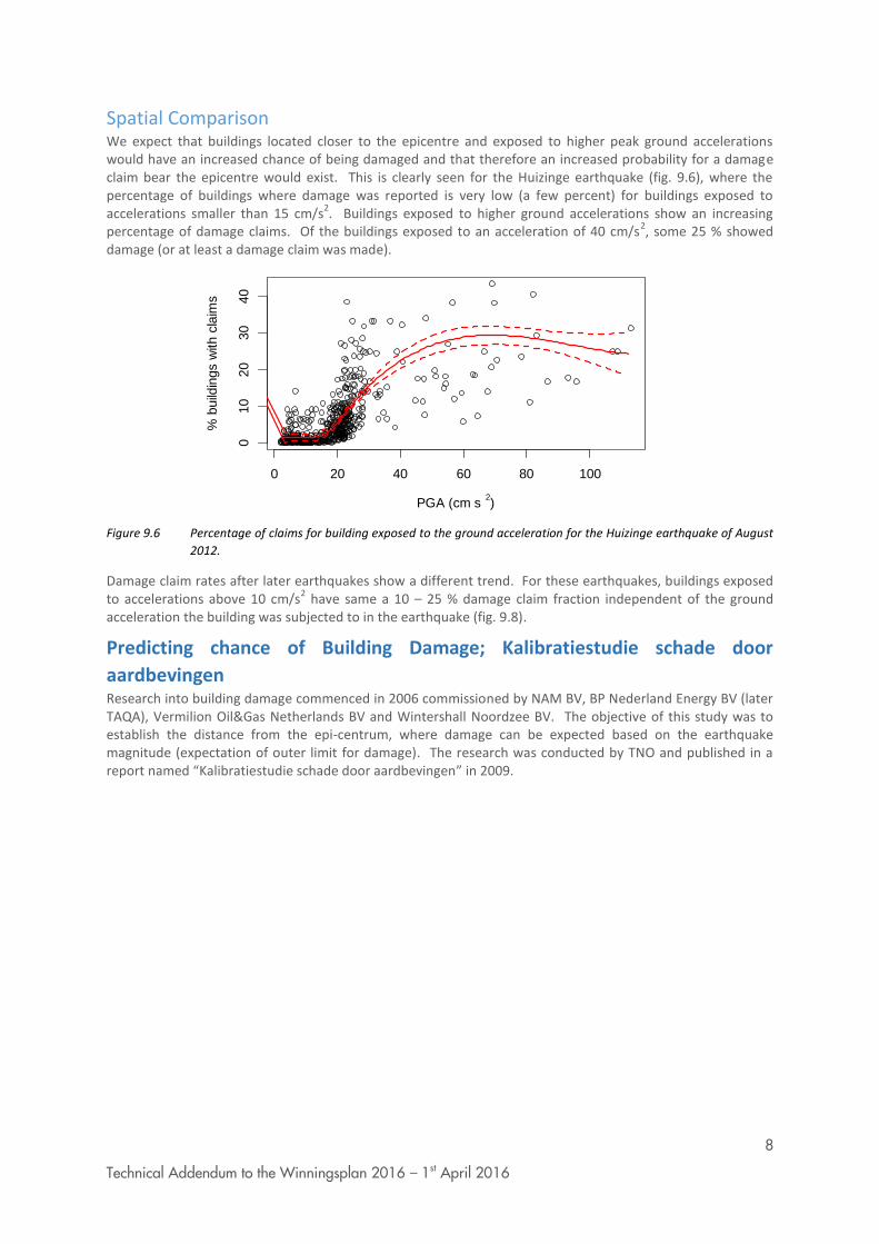
8
Technical Addendum to the Winningsplan 2016 – 1st April 2016
Spatial Comparison We expect that buildings located closer to the epicentre and exposed to higher peak ground accelerations would have an increased chance of being damaged and that therefore an increased probability for a damage claim bear the epicentre would exist. This is clearly seen for the Huizinge earthquake (fig. 9.6), where the percentage of buildings where damage was reported is very low (a few percent) for buildings exposed to accelerations smaller than 15 cm/s
2. Buildings exposed to higher ground accelerations show an increasing
percentage of damage claims. Of the buildings exposed to an acceleration of 40 cm/s2, some 25 % showed
damage (or at least a damage claim was made).
Figure 9.6 Percentage of claims for building exposed to the ground acceleration for the Huizinge earthquake of August
2012.
Damage claim rates after later earthquakes show a different trend. For these earthquakes, buildings exposed to accelerations above 10 cm/s
2 have same a 10 – 25 % damage claim fraction independent of the ground
acceleration the building was subjected to in the earthquake (fig. 9.8).
Predicting chance of Building Damage; Kalibratiestudie schade door
aardbevingen Research into building damage commenced in 2006 commissioned by NAM BV, BP Nederland Energy BV (later TAQA), Vermilion Oil&Gas Netherlands BV and Wintershall Noordzee BV. The objective of this study was to establish the distance from the epi-centrum, where damage can be expected based on the earthquake magnitude (expectation of outer limit for damage). The research was conducted by TNO and published in a report named “Kalibratiestudie schade door aardbevingen” in 2009.
0 20 40 60 80 100
010
20
30
40
PGA (cm s2)
% b
uild
ings w
ith c
laim
s
1 : gmpe_map_c1e1.csv

9
Technical Addendum to the Winningsplan 2016 – 1st April 2016
Figure 9.7 Cover of “Kalibratiestudie schade door aardbevingen” published by TNO in 2009.
Figure 9.8 Percentage of claims for building exposed to the ground acceleration for three earthquakes: Zandeweer,
Hellum and Leermens.
0 10 20 30 40 50 60 70
010
20
30
40
50
PGA (cm s2)
% b
uild
ings w
ith c
laim
s
2 : gmpe_map_c2e1.csv
10 20 30 40 50
05
10
20
30
PGA (cm s2)
% b
uild
ings w
ith c
laim
s
3 : gmpe_map_c3e1.csv
0 10 20 30 40 50
05
10
15
20
25
PGA (cm s2)
% b
uild
ings w
ith c
laim
s
5 : gmpe_map_c5e1.csv
Zandeweer
Hellum
Leermens
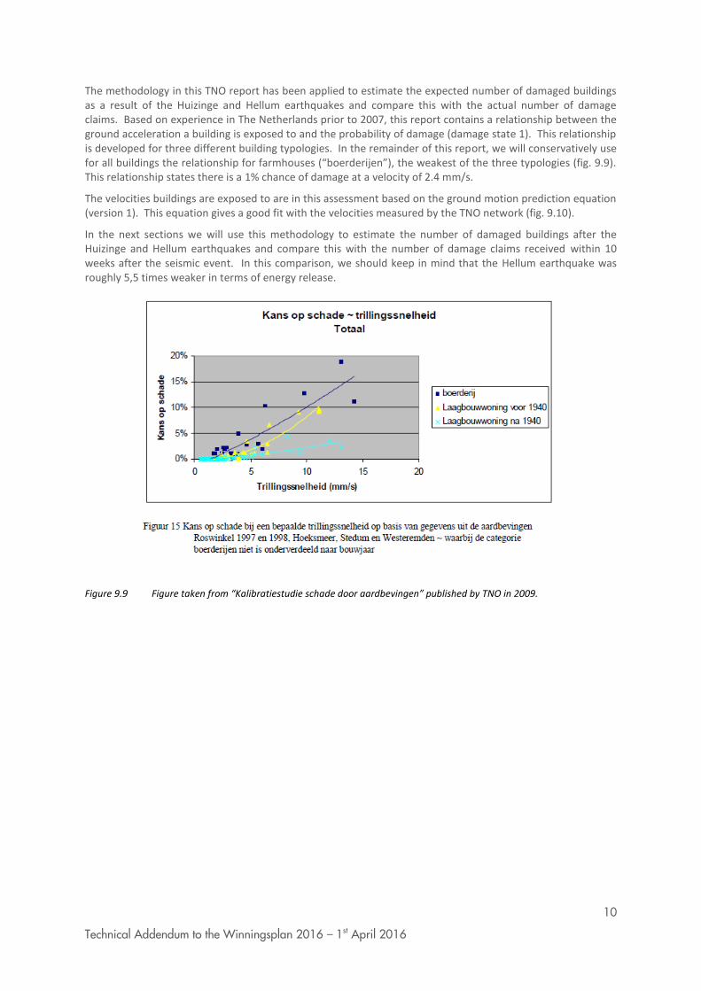
10
Technical Addendum to the Winningsplan 2016 – 1st April 2016
The methodology in this TNO report has been applied to estimate the expected number of damaged buildings as a result of the Huizinge and Hellum earthquakes and compare this with the actual number of damage claims. Based on experience in The Netherlands prior to 2007, this report contains a relationship between the ground acceleration a building is exposed to and the probability of damage (damage state 1). This relationship is developed for three different building typologies. In the remainder of this report, we will conservatively use for all buildings the relationship for farmhouses (“boerderijen”), the weakest of the three typologies (fig. 9.9). This relationship states there is a 1% chance of damage at a velocity of 2.4 mm/s.
The velocities buildings are exposed to are in this assessment based on the ground motion prediction equation (version 1). This equation gives a good fit with the velocities measured by the TNO network (fig. 9.10).
In the next sections we will use this methodology to estimate the number of damaged buildings after the Huizinge and Hellum earthquakes and compare this with the number of damage claims received within 10 weeks after the seismic event. In this comparison, we should keep in mind that the Hellum earthquake was roughly 5,5 times weaker in terms of energy release.
Figure 9.9 Figure taken from “Kalibratiestudie schade door aardbevingen” published by TNO in 2009.
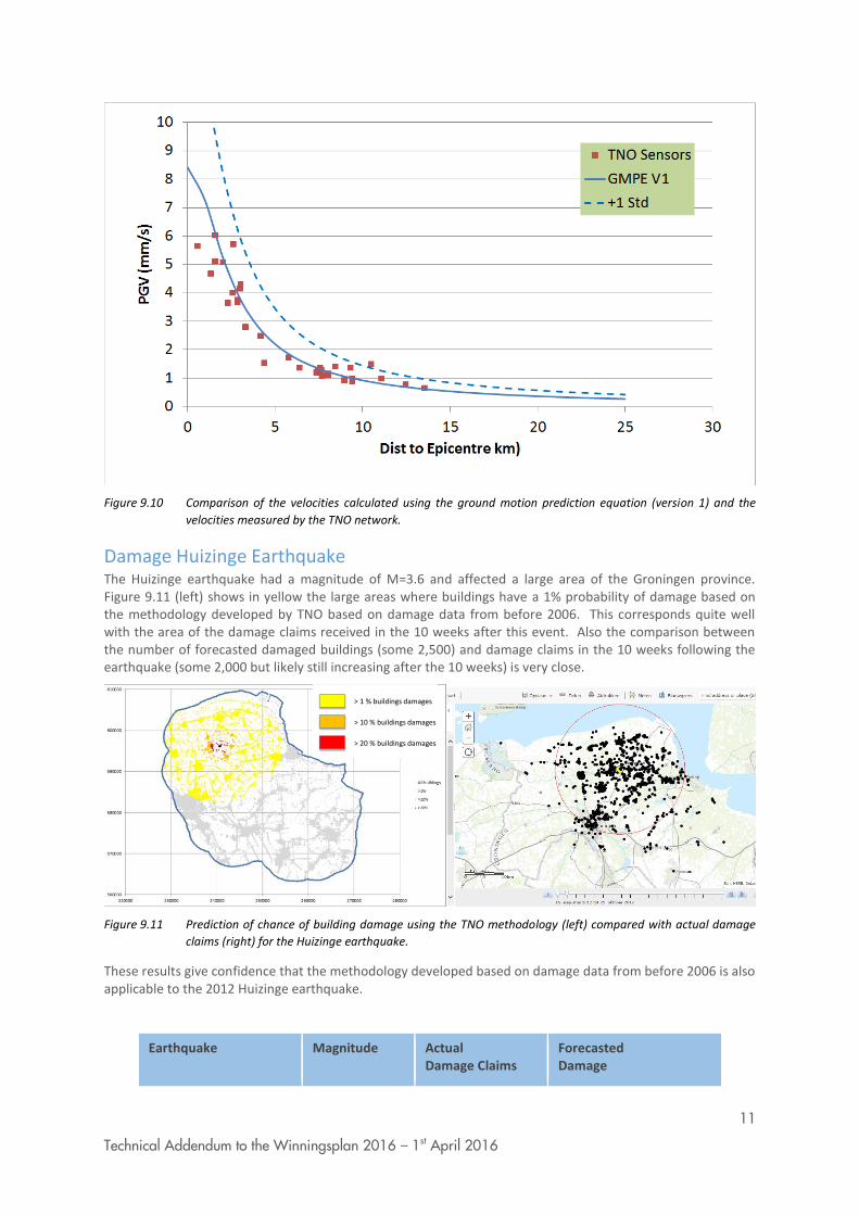
11
Technical Addendum to the Winningsplan 2016 – 1st April 2016
Figure 9.10 Comparison of the velocities calculated using the ground motion prediction equation (version 1) and the
velocities measured by the TNO network.
Damage Huizinge Earthquake The Huizinge earthquake had a magnitude of M=3.6 and affected a large area of the Groningen province. Figure 9.11 (left) shows in yellow the large areas where buildings have a 1% probability of damage based on the methodology developed by TNO based on damage data from before 2006. This corresponds quite well with the area of the damage claims received in the 10 weeks after this event. Also the comparison between the number of forecasted damaged buildings (some 2,500) and damage claims in the 10 weeks following the earthquake (some 2,000 but likely still increasing after the 10 weeks) is very close.
Figure 9.11 Prediction of chance of building damage using the TNO methodology (left) compared with actual damage
claims (right) for the Huizinge earthquake.
These results give confidence that the methodology developed based on damage data from before 2006 is also applicable to the 2012 Huizinge earthquake.
Earthquake Magnitude Actual Damage Claims
Forecasted Damage
> 1 % buildings damages
> 10 % buildings damages
> 20 % buildings damages
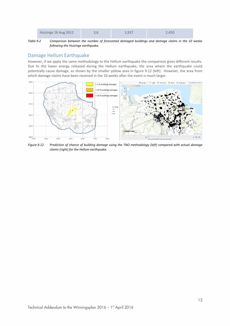
12
Technical Addendum to the Winningsplan 2016 – 1st April 2016
Huizinge 16 Aug 2012 3,6 1,937 2,450
Table 9.2 Comparison between the number of forecasted damaged buildings and damage claims in the 10 weeks
following the Huizinge earthquake.
Damage Hellum Earthquake However, if we apply the same methodology to the Hellum earthquake the comparison gives different results. Due to the lower energy released during the Hellum earthquake, the area where the earthquake could potentially cause damage, as shown by the smaller yellow area in figure 9.12 (left). However, the area from which damage claims have been received in the 10 weeks after the event is much larger.
Figure 9.12 Prediction of chance of building damage using the TNO methodology (left) compared with actual damage
claims (right) for the Hellum earthquake.
> 1 % buildings damages
> 10 % buildings damages
> 20 % buildings damages
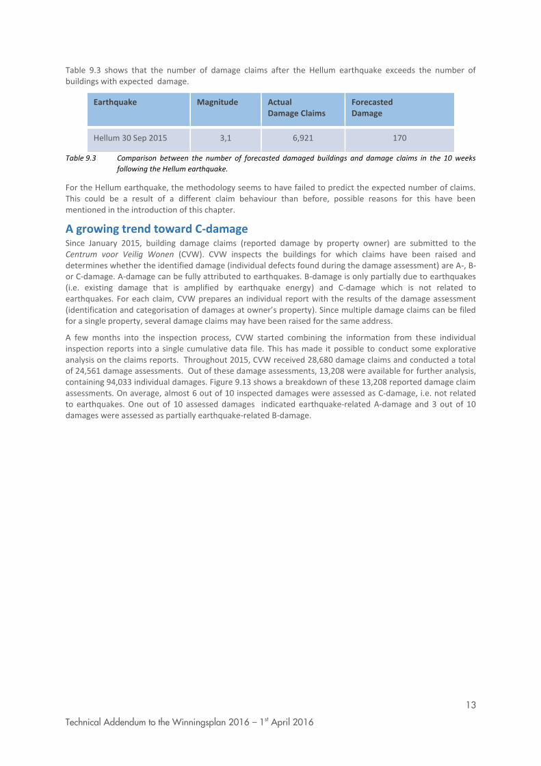
13
Technical Addendum to the Winningsplan 2016 – 1st April 2016
Table 9.3 shows that the number of damage claims after the Hellum earthquake exceeds the number of buildings with expected damage.
Earthquake Magnitude Actual Damage Claims
Forecasted Damage
Hellum 30 Sep 2015 3,1 6,921 170
Table 9.3 Comparison between the number of forecasted damaged buildings and damage claims in the 10 weeks
following the Hellum earthquake.
For the Hellum earthquake, the methodology seems to have failed to predict the expected number of claims. This could be a result of a different claim behaviour than before, possible reasons for this have been mentioned in the introduction of this chapter.
A growing trend toward C-damage Since January 2015, building damage claims (reported damage by property owner) are submitted to the Centrum voor Veilig Wonen (CVW). CVW inspects the buildings for which claims have been raised and determines whether the identified damage (individual defects found during the damage assessment) are A-, B- or C-damage. A-damage can be fully attributed to earthquakes. B-damage is only partially due to earthquakes (i.e. existing damage that is amplified by earthquake energy) and C-damage which is not related to earthquakes. For each claim, CVW prepares an individual report with the results of the damage assessment (identification and categorisation of damages at owner’s property). Since multiple damage claims can be filed for a single property, several damage claims may have been raised for the same address.
A few months into the inspection process, CVW started combining the information from these individual inspection reports into a single cumulative data file. This has made it possible to conduct some explorative analysis on the claims reports. Throughout 2015, CVW received 28,680 damage claims and conducted a total of 24,561 damage assessments. Out of these damage assessments, 13,208 were available for further analysis, containing 94,033 individual damages. Figure 9.13 shows a breakdown of these 13,208 reported damage claim assessments. On average, almost 6 out of 10 inspected damages were assessed as C-damage, i.e. not related to earthquakes. One out of 10 assessed damages indicated earthquake-related A-damage and 3 out of 10 damages were assessed as partially earthquake-related B-damage.
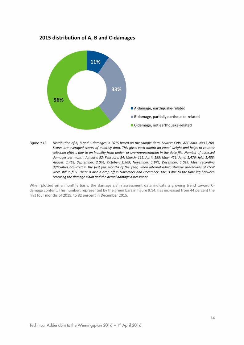
14
Technical Addendum to the Winningsplan 2016 – 1st April 2016
Figure 9.13 Distribution of A, B and C-damages in 2015 based on the sample data. Source: CVW, ABC-data. N=13,208.
Scores are averaged scores of monthly data. This gives each month an equal weight and helps to counter
selection effects due to an inability from under- or overrepresentation in the data file. Number of assessed
damages per month: January: 52; February: 54; March: 112; April: 185; May: 421; June: 1,476; July: 1,438;
August: 1,453; September: 2,044; October: 2,969; November: 1,975; December: 1,029. Most recording
difficulties occurred in the first five months of the year, when internal administrative procedures at CVW
were still in flux. There is also a drop-off in November and December. This is due to the time lag between
receiving the damage claim and the actual damage assessment.
When plotted on a monthly basis, the damage claim assessment data indicate a growing trend toward C-damage content. This number, represented by the green bars in figure 9.14, has increased from 44 percent the first four months of 2015, to 82 percent in December 2015.
11%
33%
56%
2015 distribution of A, B and C-damages
A-damage, earthquake-related
B-damage, partially earthquake-related
C-damage, not earthquake-related
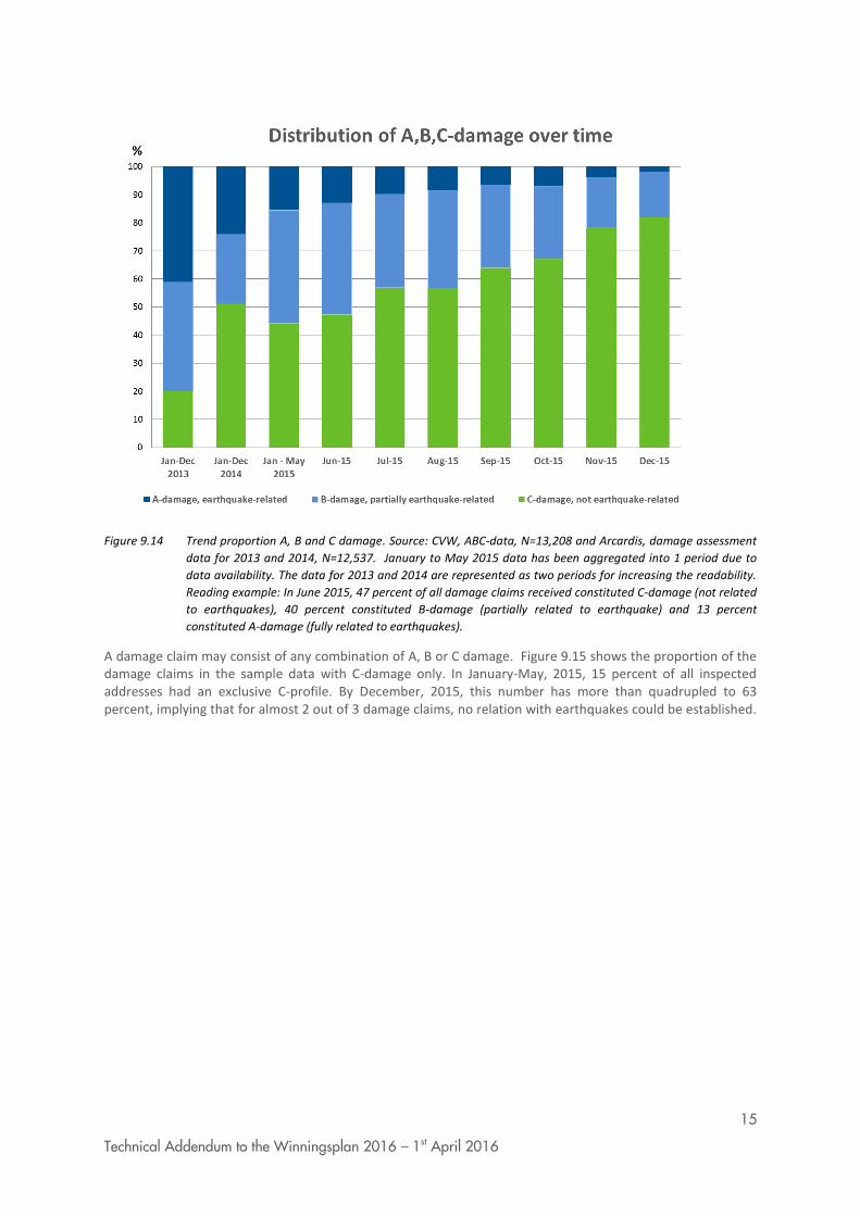
15
Technical Addendum to the Winningsplan 2016 – 1st April 2016
Figure 9.14 Trend proportion A, B and C damage. Source: CVW, ABC-data, N=13,208 and Arcardis, damage assessment
data for 2013 and 2014, N=12,537. January to May 2015 data has been aggregated into 1 period due to
data availability. The data for 2013 and 2014 are represented as two periods for increasing the readability.
Reading example: In June 2015, 47 percent of all damage claims received constituted C-damage (not related
to earthquakes), 40 percent constituted B-damage (partially related to earthquake) and 13 percent
constituted A-damage (fully related to earthquakes).
A damage claim may consist of any combination of A, B or C damage. Figure 9.15 shows the proportion of the damage claims in the sample data with C-damage only. In January-May, 2015, 15 percent of all inspected addresses had an exclusive C-profile. By December, 2015, this number has more than quadrupled to 63 percent, implying that for almost 2 out of 3 damage claims, no relation with earthquakes could be established.
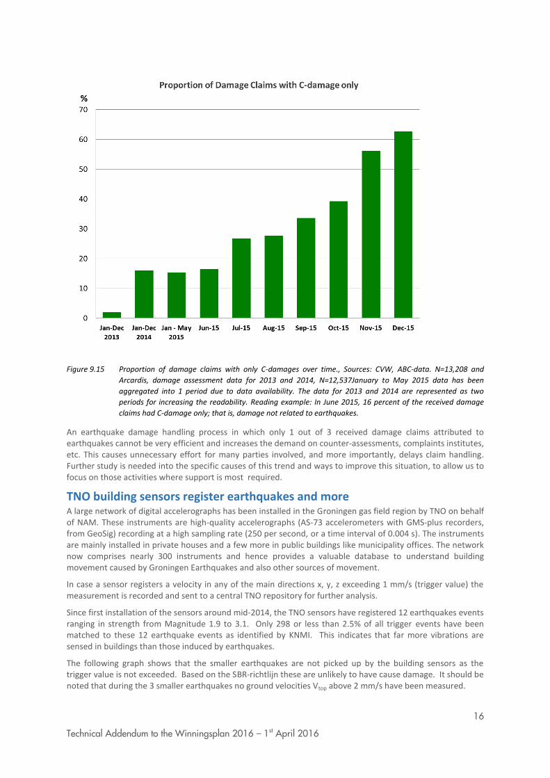
16
Technical Addendum to the Winningsplan 2016 – 1st April 2016
Figure 9.15 Proportion of damage claims with only C-damages over time., Sources: CVW, ABC-data. N=13,208 and
Arcardis, damage assessment data for 2013 and 2014, N=12,537January to May 2015 data has been
aggregated into 1 period due to data availability. The data for 2013 and 2014 are represented as two
periods for increasing the readability. Reading example: In June 2015, 16 percent of the received damage
claims had C-damage only; that is, damage not related to earthquakes.
An earthquake damage handling process in which only 1 out of 3 received damage claims attributed to earthquakes cannot be very efficient and increases the demand on counter-assessments, complaints institutes, etc. This causes unnecessary effort for many parties involved, and more importantly, delays claim handling. Further study is needed into the specific causes of this trend and ways to improve this situation, to allow us to focus on those activities where support is most required.
TNO building sensors register earthquakes and more A large network of digital accelerographs has been installed in the Groningen gas field region by TNO on behalf of NAM. These instruments are high-quality accelerographs (AS-73 accelerometers with GMS-plus recorders, from GeoSig) recording at a high sampling rate (250 per second, or a time interval of 0.004 s). The instruments are mainly installed in private houses and a few more in public buildings like municipality offices. The network now comprises nearly 300 instruments and hence provides a valuable database to understand building movement caused by Groningen Earthquakes and also other sources of movement.
In case a sensor registers a velocity in any of the main directions x, y, z exceeding 1 mm/s (trigger value) the measurement is recorded and sent to a central TNO repository for further analysis.
Since first installation of the sensors around mid-2014, the TNO sensors have registered 12 earthquakes events ranging in strength from Magnitude 1.9 to 3.1. Only 298 or less than 2.5% of all trigger events have been matched to these 12 earthquake events as identified by KNMI. This indicates that far more vibrations are sensed in buildings than those induced by earthquakes.
The following graph shows that the smaller earthquakes are not picked up by the building sensors as the trigger value is not exceeded. Based on the SBR-richtlijn these are unlikely to have cause damage. It should be noted that during the 3 smaller earthquakes no ground velocities Vtop above 2 mm/s have been measured.
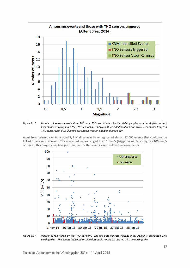
17
Technical Addendum to the Winningsplan 2016 – 1st April 2016
Figure 9.16 Number of seismic events since 10th
June 2014 as detected by the KNMI geophone network (bleu – bar).
Events that also triggered the TNO sensors are shown with an additional red bar, while events that trigger a
TNO sensor with Vtop> 2 mm/s are shown with an additional green bar.
Apart from seismic events, around 2/3 of all sensors have registered almost 12,000 events that could not be linked to any seismic event. The measured values ranged from 1 mm/s (trigger value) to as high as 100 mm/s or more. This range is much larger than that for the seismic event related measurements.
Figure 9.17 Velocoites registered by the TNO network. The red dots indicate velocity measurements associated with
earthquakes. The events indicated by blue dots could not be associated with an earthquake.
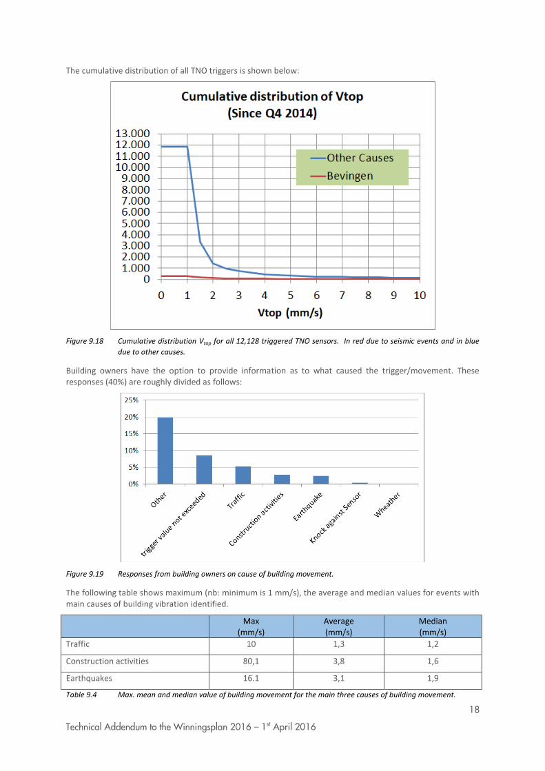
18
Technical Addendum to the Winningsplan 2016 – 1st April 2016
The cumulative distribution of all TNO triggers is shown below:
Figure 9.18 Cumulative distribution Vtop for all 12,128 triggered TNO sensors. In red due to seismic events and in blue
due to other causes.
Building owners have the option to provide information as to what caused the trigger/movement. These responses (40%) are roughly divided as follows:
Figure 9.19 Responses from building owners on cause of building movement.
The following table shows maximum (nb: minimum is 1 mm/s), the average and median values for events with main causes of building vibration identified.
Max (mm/s)
Average (mm/s)
Median (mm/s)
Traffic 10 1,3 1,2
Construction activities 80,1 3,8 1,6
Earthquakes 16.1 3,1 1,9
Table 9.4 Max. mean and median value of building movement for the main three causes of building movement.
19
Technical Addendum to the Winningsplan 2016 – 1st April 2016
The above information clearly demonstrates that buildings in the Groningen earthquake area (or anywhere else) are subject to movement on a regular basis due to non-earthquake related causes, especially in the range below ca. 3 mm/s. It is therefore unlikely that the movement of the buildings to earthquakes with magnitude smaller than M=2 will contribute significantly to building damage.
Conclusions A simple forecasting method for D1 damage state, based on 2009 Kalibratiestudie by TNO/KNMI, was used
to forecast the chance of damage based on hazard data. These forecasts were compared with historical damage claim data (period 2012- 2015). This study is calibrated on damage data from before 2007 and also provides good results for building damage (claims) for the Huizinge 2012 earthquake. However, for earthquakes after 2012, this method is not able to match building damage claims.
The relationship between seismic activity and damage claims appears to be complex.
Empirical evidence pointing to strong increase in the number of claims post-Huizinge (early-2013).
Further research is required into: o The area where earthquakes could release sufficient energy to cause damage o the precise relationship between damage claim reports and actual damage, o The assessment of claimed damages as A-, B- or C-damage, or combinations thereof
There appears a growing trend in the content of C-damage (damage which cannot be attributed to earthquakes) in damage claims from mid-2015 onwards.
The TNO sensors show that buildings in Groningen experience movements due to a wide variety of causes. Traffic and construction work also cause building movement.

20
Technical Addendum to the Winningsplan 2016 – 1st April 2016
Appendix A - Spectral Hazard Maps
Figure A.1 Mean spectral hazard maps with an average 0.2% annual chance of exceedance (1 in 475 years) from 2016
to 2017 given the V2 linear compaction model and the 27 bcm production plan. Mean hazard was computed
according to the 9 branches of the logic tree representing epsitemic uncertainty in the seismological and
ground motion models.
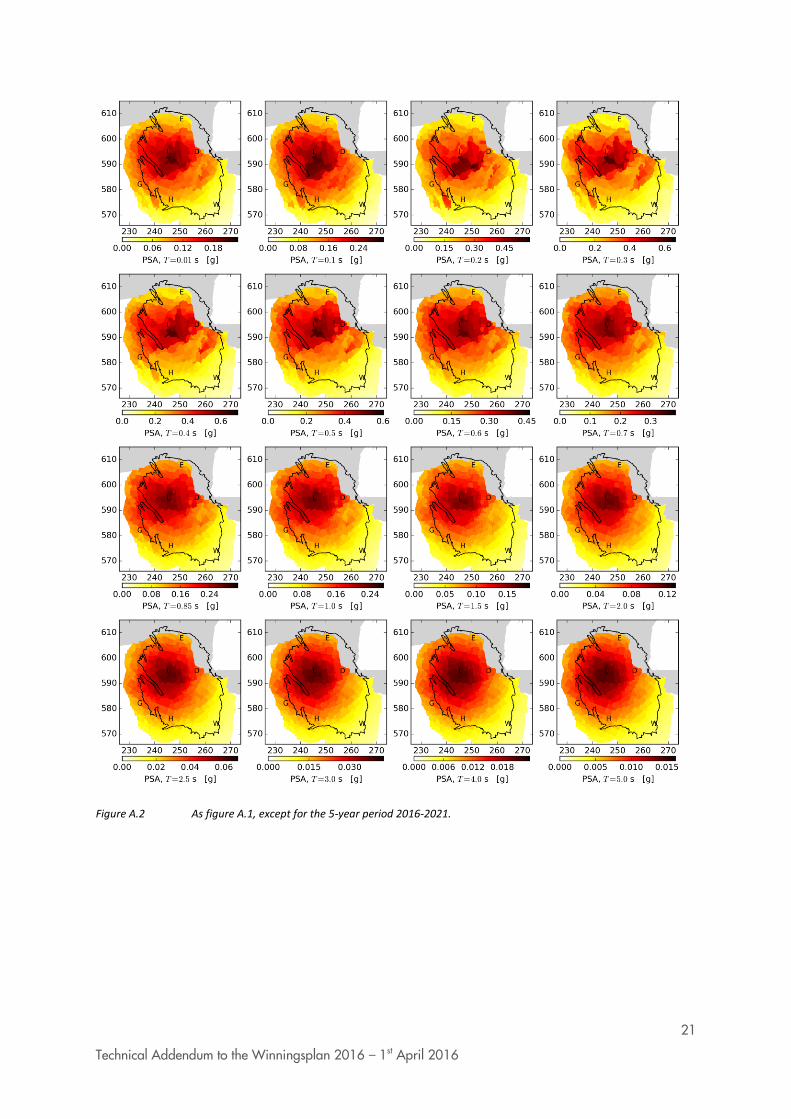
21
Technical Addendum to the Winningsplan 2016 – 1st April 2016
Figure A.2 As figure A.1, except for the 5-year period 2016-2021.
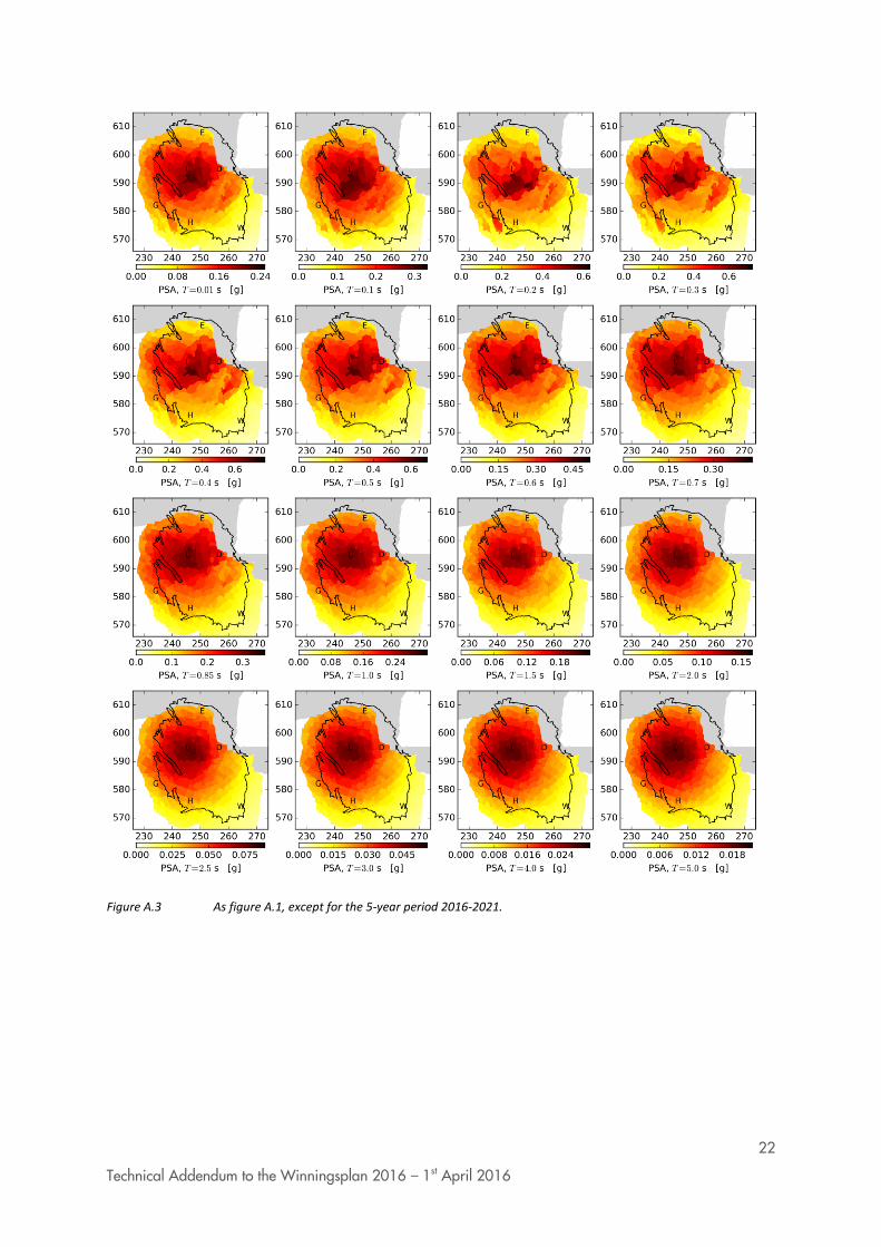
22
Technical Addendum to the Winningsplan 2016 – 1st April 2016
Figure A.3 As figure A.1, except for the 5-year period 2016-2021.
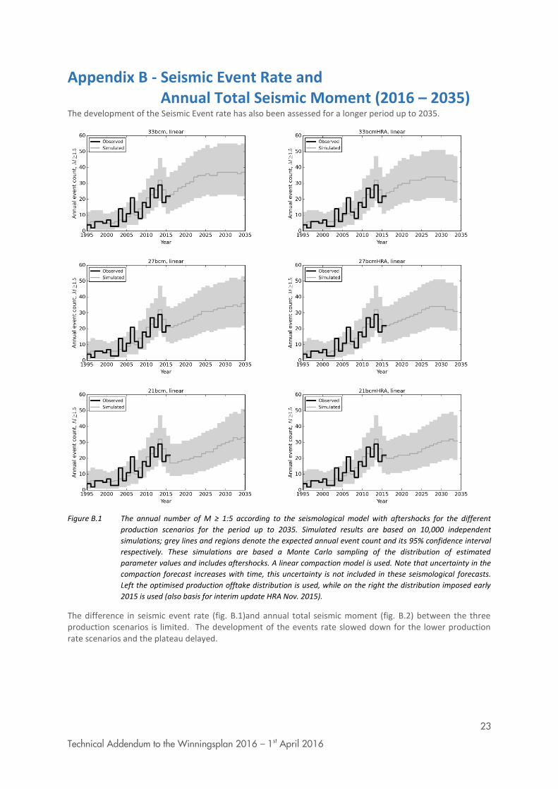
23
Technical Addendum to the Winningsplan 2016 – 1st April 2016
Appendix B - Seismic Event Rate and Annual Total Seismic Moment (2016 – 2035)
The development of the Seismic Event rate has also been assessed for a longer period up to 2035.
Figure B.1 The annual number of M ≥ 1:5 according to the seismological model with aftershocks for the different
production scenarios for the period up to 2035. Simulated results are based on 10,000 independent
simulations; grey lines and regions denote the expected annual event count and its 95% confidence interval
respectively. These simulations are based a Monte Carlo sampling of the distribution of estimated
parameter values and includes aftershocks. A linear compaction model is used. Note that uncertainty in the
compaction forecast increases with time, this uncertainty is not included in these seismological forecasts.
Left the optimised production offtake distribution is used, while on the right the distribution imposed early
2015 is used (also basis for interim update HRA Nov. 2015).
The difference in seismic event rate (fig. B.1)and annual total seismic moment (fig. B.2) between the three production scenarios is limited. The development of the events rate slowed down for the lower production rate scenarios and the plateau delayed.
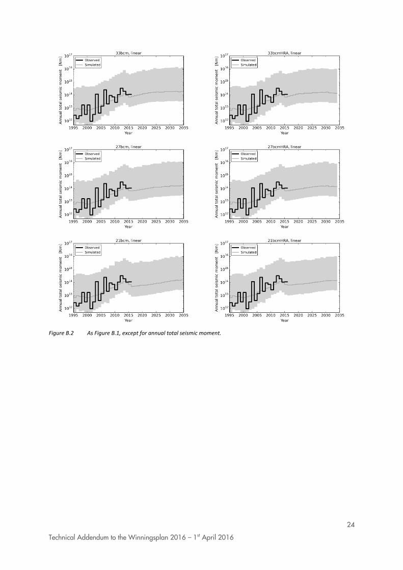
24
Technical Addendum to the Winningsplan 2016 – 1st April 2016
Figure B.2 As Figure B.1, except for annual total seismic moment.

25
Technical Addendum to the Winningsplan 2016 – 1st April 2016
Appendix C – Hazard Maps Large Format
Assessment period: 2016-2021
Exceedance probability: 0.2%/year
Production scenario: 33 bcm (optimized)
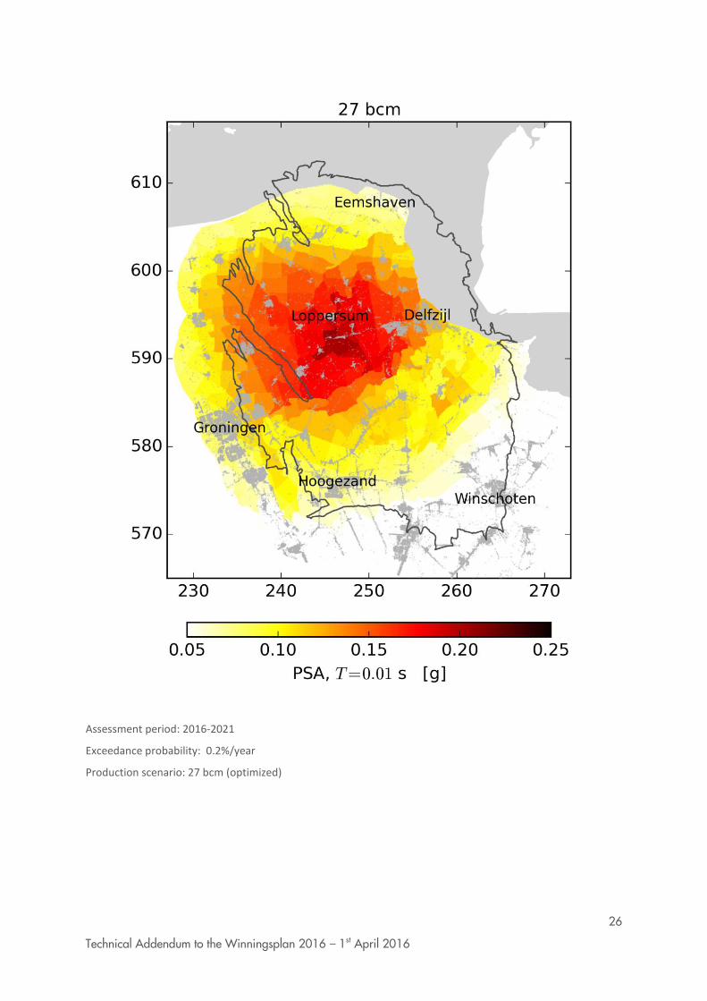
26
Technical Addendum to the Winningsplan 2016 – 1st April 2016
Assessment period: 2016-2021
Exceedance probability: 0.2%/year
Production scenario: 27 bcm (optimized)
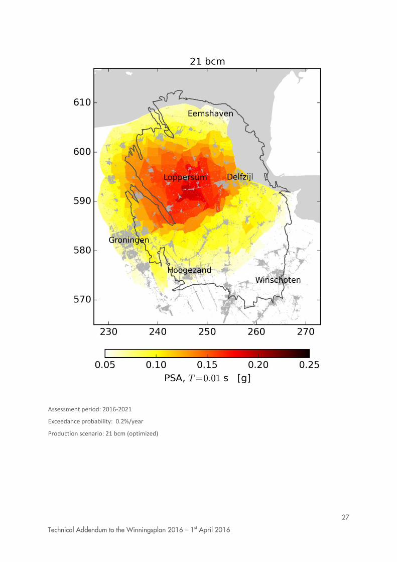
27
Technical Addendum to the Winningsplan 2016 – 1st April 2016
Assessment period: 2016-2021
Exceedance probability: 0.2%/year
Production scenario: 21 bcm (optimized)
28
Technical Addendum to the Winningsplan 2016 – 1st April 2016
References E.J. den Haan, Het a,b,c –Isotachenmodel: hoeksteen van een nieuwe aanpak van zettingsberekeningen, Geotechniek, oktober 2003
de Waal, J.A. (1986). On the rate type compaction behaviour of sandstone reservoir rock. PhD thesis, Technische Hogeschool, Delft.
Geertsma, J. (1973) , Land Subsidence Above Compacting Oil and Gas Reservoirs, J. Petr. Tech., pp.734-744.
Geertsma, J. and van Opstal, G. (1973). A Numerical Technique for Predicting Subsidence Above Compacting Reservoirs, Based on the Nucleus of Strain Concept. Verh. Kon. Ned. Geol. Mijnbouwk. Gen., 28, pp. 63-78.
NAM (2011) Subsurface Technical Report Subsidence Modelling of Ameland Fields. UIE Report No: EP201105208617
NAM (2015) Bodemdaling door aardgaswinning. Statusrapport 2015 en prognose tot het jaar 2080. NAM rapport EP201511213444
TNO (2013) A general framework for rate dependent compaction models for reservoir rock. TNO 2013 R11405
List of abbreviations TNO Nederlandse Organisatie voor toegepast-natuurwetenschappelijk onderzoek, Netherlands
Organisation for Applied Scientific Research
ARPR Annual Review of Petroleum Recources
GFR2015 Groningen Field Review 2015
RMS Root Mean Square
PVT Fluid behaviour as a function of Pressure, Volume and Temperature
HRA Hazard and Risk Assessment
RFT Repeat Formation Tester
SPTG Static Pressure and Temperature Measurement
GWC Gas Water Contact
PNL Pulse Neutron Log
CITHP Closed in tubing head pressures
BU Build-up
UR Ultimate recovery
NorGroN Norg-Groningen pipeline
(N.)Bcm N.Bcm refers to a volume of a billion normal cubic meters. Normal means the volume is measured at a standard temperature (0 ᵒC) and pressure (1 bar).

29
Technical Addendum to the Winningsplan 2016 – 1st April 2016