Te Kura M atai Tatauranga -...
45
School of Mathematics and Statistics Te Kura M¯atai Tatauranga Lab Guide — Probability & Simulation with R The aim of this lab guide is to introduce you to basic probability/simulation with the statistical computing language R. Contents 1 Discrete Random Variables in R 3 1.1 Binomial Distribution ................................. 4 1.2 Geometric Distribution ................................. 6 1.3 Negative Binomial Distribution ............................ 8 1.4 Poisson Distribution .................................. 10 2 Continuous Random Variables with R 12 2.1 Uniform Distribution .................................. 13 2.2 Lifetime Models ..................................... 16 2.2.1 Exponential Distribution ........................... 16 2.3 Gamma Distribution .................................. 18 2.4 Sampling distributions ................................. 19 2.4.1 Normal (or Gaussian) Distribution ...................... 20 2.4.2 χ 2 Distribution ................................. 21 2.4.3 Student’s t Distribution ............................ 22 3 Random Generators 24 3.1 Congruential Random Generators ........................... 24 3.2 Seeding ......................................... 24 4 Simulating Discrete Random Variables 25 4.1 Example: Binomial Random Variable ........................ 26 4.2 Sequence of independent trials ............................ 27 4.3 Example: Geometric Random Variable ........................ 27 4.4 Example: Negative Binomial Random Variable ................... 28 5 Simulating Continuous Random Variables 28 5.1 Inverse Transformation Method (ITM) ........................ 28 SCIE2017 1 Probability & Simulation with R
-
Upload
nguyentram -
Category
Documents
-
view
219 -
download
1
Transcript of Te Kura M atai Tatauranga -...

School of Mathematics and StatisticsTe Kura Matai Tatauranga
Lab Guide — Probability & Simulation with R
The aim of this lab guide is to introduce you to basic probability/simulation with the statisticalcomputing language R.
Contents
1 Discrete Random Variables in R 3
1.1 Binomial Distribution . . . . . . . . . . . . . . . . . . . . . . . . . . . . . . . . . 4
1.2 Geometric Distribution . . . . . . . . . . . . . . . . . . . . . . . . . . . . . . . . . 6
1.3 Negative Binomial Distribution . . . . . . . . . . . . . . . . . . . . . . . . . . . . 8
1.4 Poisson Distribution . . . . . . . . . . . . . . . . . . . . . . . . . . . . . . . . . . 10
2 Continuous Random Variables with R 12
2.1 Uniform Distribution . . . . . . . . . . . . . . . . . . . . . . . . . . . . . . . . . . 13
2.2 Lifetime Models . . . . . . . . . . . . . . . . . . . . . . . . . . . . . . . . . . . . . 16
2.2.1 Exponential Distribution . . . . . . . . . . . . . . . . . . . . . . . . . . . 16
2.3 Gamma Distribution . . . . . . . . . . . . . . . . . . . . . . . . . . . . . . . . . . 18
2.4 Sampling distributions . . . . . . . . . . . . . . . . . . . . . . . . . . . . . . . . . 19
2.4.1 Normal (or Gaussian) Distribution . . . . . . . . . . . . . . . . . . . . . . 20
2.4.2 χ2 Distribution . . . . . . . . . . . . . . . . . . . . . . . . . . . . . . . . . 21
2.4.3 Student’s t Distribution . . . . . . . . . . . . . . . . . . . . . . . . . . . . 22
3 Random Generators 24
3.1 Congruential Random Generators . . . . . . . . . . . . . . . . . . . . . . . . . . . 24
3.2 Seeding . . . . . . . . . . . . . . . . . . . . . . . . . . . . . . . . . . . . . . . . . 24
4 Simulating Discrete Random Variables 25
4.1 Example: Binomial Random Variable . . . . . . . . . . . . . . . . . . . . . . . . 26
4.2 Sequence of independent trials . . . . . . . . . . . . . . . . . . . . . . . . . . . . 27
4.3 Example: Geometric Random Variable . . . . . . . . . . . . . . . . . . . . . . . . 27
4.4 Example: Negative Binomial Random Variable . . . . . . . . . . . . . . . . . . . 28
5 Simulating Continuous Random Variables 28
5.1 Inverse Transformation Method (ITM) . . . . . . . . . . . . . . . . . . . . . . . . 28
SCIE2017 1 Probability & Simulation with R
6 Practice Problems with R 31
6.1 Monty Hall Game . . . . . . . . . . . . . . . . . . . . . . . . . . . . . . . . . . . 31
6.2 Project Selection (OPTIONAL) . . . . . . . . . . . . . . . . . . . . . . . . . . . . 34
6.3 Simulate M/M/1 . . . . . . . . . . . . . . . . . . . . . . . . . . . . . . . . . . . . 36
7 Practice Problems 39
SCIE2017 2 Probability & Simulation with R
1 Discrete Random Variables in R
Recommended Reading:
The notes follow Owen Jones, RobertMaillardet, and Andrew Robinson, Sci-entific Programming and SimulationUsing R, Chapter 15, §15.1 to and§15.6
We use R in this course because it knows a lot about probability (e.g.,probability distribution functions (pdf) and cumulative distribution func-tions (cdf) of many distributions), and makes it very easy to use vectorsand matrices.
R has built-in functions for most commonly encountered probability distri-butions. Suppose that the random variable X has a dist distribution withparameters p1, p2, . . . then
> ddist(x, p1, p2, ...)
is the P (X = x) for discrete X, or the value of the density function f(x)at x for continuous X. The result of
> pdist(x, p1, p2, ...)
is equal to FX(x) = P (X ≤ x), i.e., the value of the cdf function at x.
> qdist(p, p1, p2, ...)
is equal to the smallest q for which P (X ≤ q) ≥ p, i.e., the 100 p% −percentile.
> rdist(n, p1, p2, ...)
is a vector of n pseudo-random numbers from distribution dist (or a vectorof n variates/observations of X). The inputs x, q, p can be vector valued,therefore the output is also vector valued. In Table 1 some of the discretedistributions in R, with their parameters are listed.
SCIE2017 3 Probability & Simulation with R
Table 1: Some Discrete Distributions in R
Distribution R name (dist) Parameter names
Binomial binom size, probGeometric geom probNegative Binomial nbinom size, probPoisson pois ratehypergeometric hyper m, n, k
1.1 Binomial Distribution
Let X be the number of successes in n independent trials, with probabilityof success p, then X has a binomial distribution with parameters n and p,X ∼ binom(n, p).
■ Note : Bernoulli Distribution Bernoulli distribution is thesame as binomial distribution with parameter n = 1, i.e., B ∼Bernoulli(p) is equivalent toB ∼ binom(1, p). The mass probability mass function (pmf) of Bis
P (B = x) =
{p forx = 1
1− p forx = 0
and corresponding mean value and variance are
E(B) = p and V ar(B) = p(1− p).
A single draw from Bernoulli(p) distribution is called aBernoulli trial. If the observed value is B = 1 we say thatthe trial was a success, otherwise the trial was a failure.
Therefore, if B1, B2, . . . , Bn are independent identically distributed (iid)Bernoulli random variables with parameter p, i.e., each of them havingvalue of either 0 or 1, then
X = B1 +B2 + . . .+Bn
SCIE2017 4 Probability & Simulation with R
will represent the number of 1′s, i.e., the number of successes out of ntrials. The possible values of X are x = 0, 1, . . . , n with correspondingprobabilities
P (X = x) =
(n
k
)px(1− p)n−x,
andE(X) = np and V ar(X) = np(1− p).
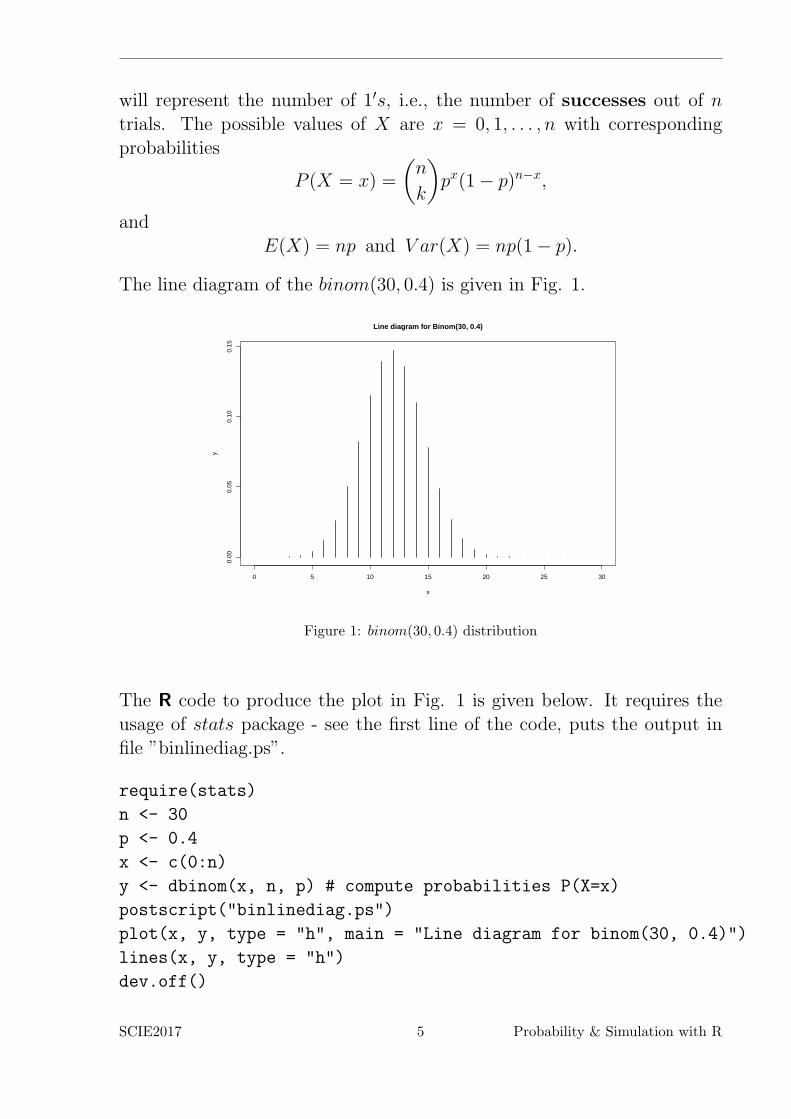
The line diagram of the binom(30, 0.4) is given in Fig. 1.
0 5 10 15 20 25 30
0.00
0.05
0.10
0.15
Line diagram for Binom(30, 0.4)
x
y
Figure 1: binom(30, 0.4) distribution
The R code to produce the plot in Fig. 1 is given below. It requires theusage of stats package - see the first line of the code, puts the output infile ”binlinediag.ps”.
require(stats)
n <- 30
p <- 0.4
x <- c(0:n)
y <- dbinom(x, n, p) # compute probabilities P(X=x)
postscript("binlinediag.ps")
plot(x, y, type = "h", main = "Line diagram for binom(30, 0.4)")
lines(x, y, type = "h")
dev.off()
SCIE2017 5 Probability & Simulation with R
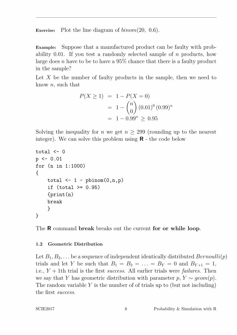
Exercise: Plot the line diagram of binom(20, 0.6).
Example: Suppose that a manufactured product can be faulty with prob-ability 0.01. If you test a randomly selected sample of n products, howlarge does n have to be to have a 95% chance that there is a faulty productin the sample?
Let X be the number of faulty products in the sample, then we need toknow n, such that
P (X ≥ 1) = 1− P (X = 0)
= 1−(n
0
)(0.01)0 (0.99)n
= 1− 0.99n ≥ 0.95
Solving the inequality for n we get n ≥ 299 (rounding up to the nearestinteger). We can solve this problem using R - the code below
total <- 0
p <- 0.01
for (n in 1:1000)
{
total <- 1 - pbinom(0,n,p)
if (total >= 0.95)
{print(n)
break
}
}
The R command break breaks out the current for or while loop.
1.2 Geometric Distribution
LetB1, B2, . . . be a sequence of independent identically distributedBernoulli(p)trials and let Y be such that B1 = B2 = . . . = BY = 0 and BY+1 = 1,i.e., Y + 1th trial is the first success. All earlier trials were failures. Thenwe say that Y has geometric distribution with parameter p, Y ∼ geom(p).The random variable Y is the number of of trials up to (but not including)the first success.
SCIE2017 6 Probability & Simulation with R
The possible values of Y ∼ geom(p) are y = 0, 1, . . . , with correspondingprobabilities
P (Y = y) = (1− p)y p
and
E(X) =1− p
pand V ar(X) =
1− p
p2.
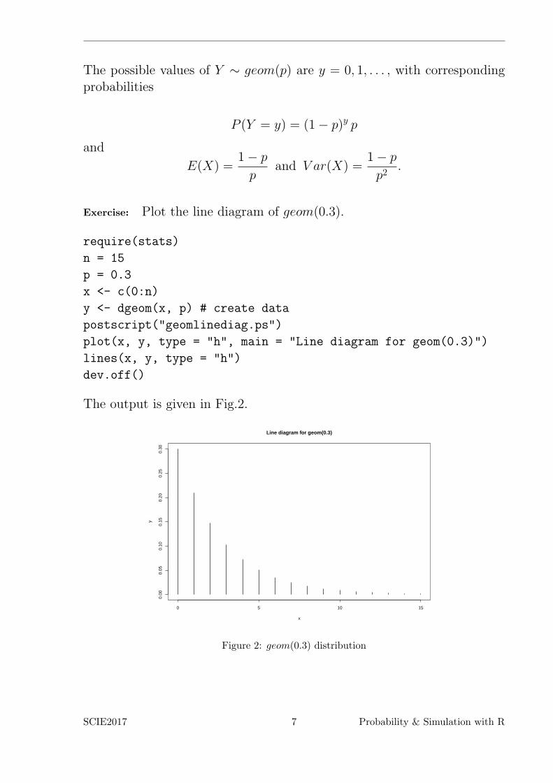
Exercise: Plot the line diagram of geom(0.3).
require(stats)
n = 15
p = 0.3
x <- c(0:n)
y <- dgeom(x, p) # create data
postscript("geomlinediag.ps")
plot(x, y, type = "h", main = "Line diagram for geom(0.3)")
lines(x, y, type = "h")
dev.off()
The output is given in Fig.2.
0 5 10 15
0.00
0.05
0.10
0.15
0.20
0.25
0.30
Line diagram for geom(0.3)
x
y
Figure 2: geom(0.3) distribution
SCIE2017 7 Probability & Simulation with R
Exercise: Plot the line graph of geom(0.3). Include only possible values yof Y such that P (Y = y) > 0.00001.
Example: You are trying to light a barbeque with matches on a windy day.Each match has a chance of p = 0.1 of lighting the barbeque and you haveonly 4 matches. What is the probability you get the barbeque lit beforeyou run out of matches?
Let Y be the number of failed attempts before you light the barbeque.Then Y ∼ geom(0.1) and the required probability is
P (Y ≤ 3) = 1− (1− 0.1)4
= 0.3439
> pgeom(3, 0.1)
[1] 0.3439
Is it better to use the matches two at the time if the probability of suc-cessfully lighting the barbeque increases to 0.3? We have
> pgeom(1, 0.3)
[1] 0.51
So, we should use the matches two at the time.
1.3 Negative Binomial Distribution
Let Z be the number of trials before the rth success, in a sequence of iidBernoulli(p) trials. Then Z has a negative binomial distribution with pa-rameters r and p, i.e., Z ∼ nbinom(r, p). Let Y1, Y2, . . . , Yr be iid geom(p)random variables. Then
Z = Y1 + Y2 + . . .+ Yr ∼ nbinom(r, p).
For z = 0, 1, . . . ,
P (Z = z) =
(r + z − 1
r − 1
)pr(1− p)z,
and
E(Z) =r(1− p)
pand V ar(Z) =
r(1− p)
p2.
SCIE2017 8 Probability & Simulation with R
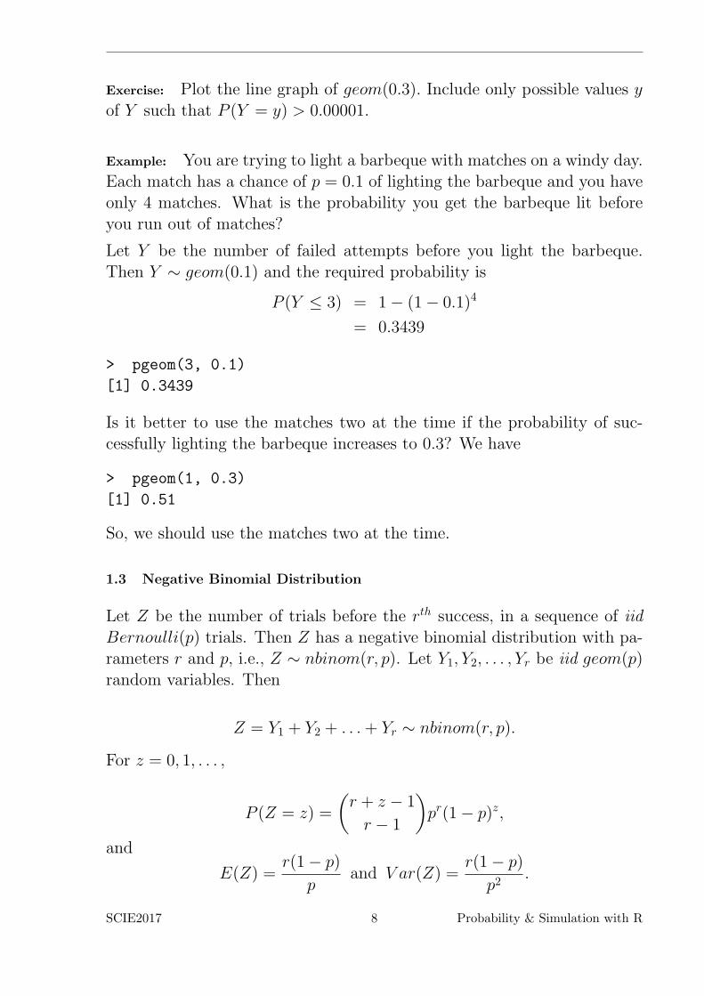
The line diagram for nbinom(3, 0.3) is given in Fig. 3.
0 5 10 15 20 25 30
0.00
0.02
0.04
0.06
0.08
0.10
Line diagram for nbinom(3, 0.3)
x
y
Figure 3: nbinom(3, 0.3) distribution
Example: A manufacturer is testing the quality of its products by ran-domly selecting 100 from each batch. If there are more than 3 faultyitems, then the production is stopped and an attempt to fix the problemis made.
Suppose that the items are independent and each of them is faulty withprobability p. Let X be the number of faults in a sample of size 100, thenX ∼ binom(100, p). Then
P (stopping production) = P (X ≥ 3).
If p = 0.01 then that probability of stopping production is
> 1 - pbinom(2,100, 0.01)
[1] 0.0793732
In practice, we usually test sequentially and stop when three faulty itemsare found. Let Z be the number of items we test before we find threefaults, then Z ∼ nbinom(3, p) and
P (stopping production) = P (Z + 3 ≤ 100).
Note that Z + 3 is the total number of tests up to and including the thirdfault. In R we have
SCIE2017 9 Probability & Simulation with R
> pnbinom(97,3,0.01)
[1] 0.0793732
Exercise: Write an R code to plot the line diagram of nbinom(3, 0.3), asgiven in Fig. 3.
1.4 Poisson Distribution
If X has a Poisson distribution with parameter λ, X ∼ pois(λ), then forx = 0, 1, . . . , the corresponding probability mass distribution function is
P (X = x) =λxe−λx
x!,
andE(X) = λ and V ar(X) = λ
x! is called x factorial. Recall that 0! = 1 and for x > 1, x! = 1×2×3 . . . x.
There is an R built-in function for x factorial. The function gamma(x+1)is x!. For example, 5! = 120, same as below
> gamma(5+1)
[1] 120
The Poisson distribution is used to model rare events, and events occurringat random over time and space, e.g., number of accidents in a year; thenumber of typos on a page; the number of phone calls arriving in a callcenter within an hour.
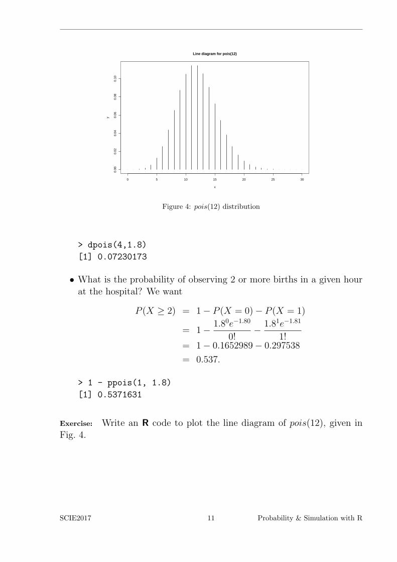
The line diagram for pois(12) is given in Fig. 4.
Example: Births in a hospital occur randomly at an average rate of 1.8births per hour. Let X be the number of births in a given hour.
• What is the probability of observing 4 births in a given hour at thehospital?
The births occur randomly, therefore X ∼ pois(1.8). Then
P (X = 4) =1.84e−1.84
4!= 0.0723.
SCIE2017 10 Probability & Simulation with R
0 5 10 15 20 25 30
0.00
0.02
0.04
0.06
0.08
0.10
Line diagram for pois(12)
x
y
Figure 4: pois(12) distribution
> dpois(4,1.8)
[1] 0.07230173
• What is the probability of observing 2 or more births in a given hourat the hospital? We want
P (X ≥ 2) = 1− P (X = 0)− P (X = 1)
= 1− 1.80e−1.80
0!− 1.81e−1.81
1!= 1− 0.1652989− 0.297538
= 0.537.
> 1 - ppois(1, 1.8)
[1] 0.5371631
Exercise: Write an R code to plot the line diagram of pois(12), given inFig. 4.
SCIE2017 11 Probability & Simulation with R
2 Continuous Random Variables with R
Recommended Reading:
The notes follow Owen Jones, RobertMaillardet, and Andrew Robinson, Sci-entific Programming and SimulationUsing R, Chapter 16, §16.1 to and§16.5
We use R in this course because it knows a lot about probability (e.g., pdfsand cdfs of many distributions), and makes it very easy to use vectors andmatrices.
R has built-in functions for most commonly encountered probability dis-tributions. Suppose that the random variable X has dist distribution withparameters p1, p2, . . . then
> ddist(x, p1, p2, ...)
is the P (X = x) for discrete X, or the value of the probability densityfunction (pdf) f(x) of X at x for continuous X.
> pdist(x, p1, p2, ...)
is equal to F (x) = P (X ≤ x), which is the cumulative distribution function(cdf) of X.
> qdist(p, p1, p2, ...)
is equal to the smallest q for which P (X ≤ q) ≥ p, i.e., the 100p% −percentile.
> rdist(n, p1, p2, ...)
is a vector of n pseudo-random numbers from distribution dist. The inputsx, q, p can be vector valued, therefore the output is also vector valued. In
SCIE2017 12 Probability & Simulation with R
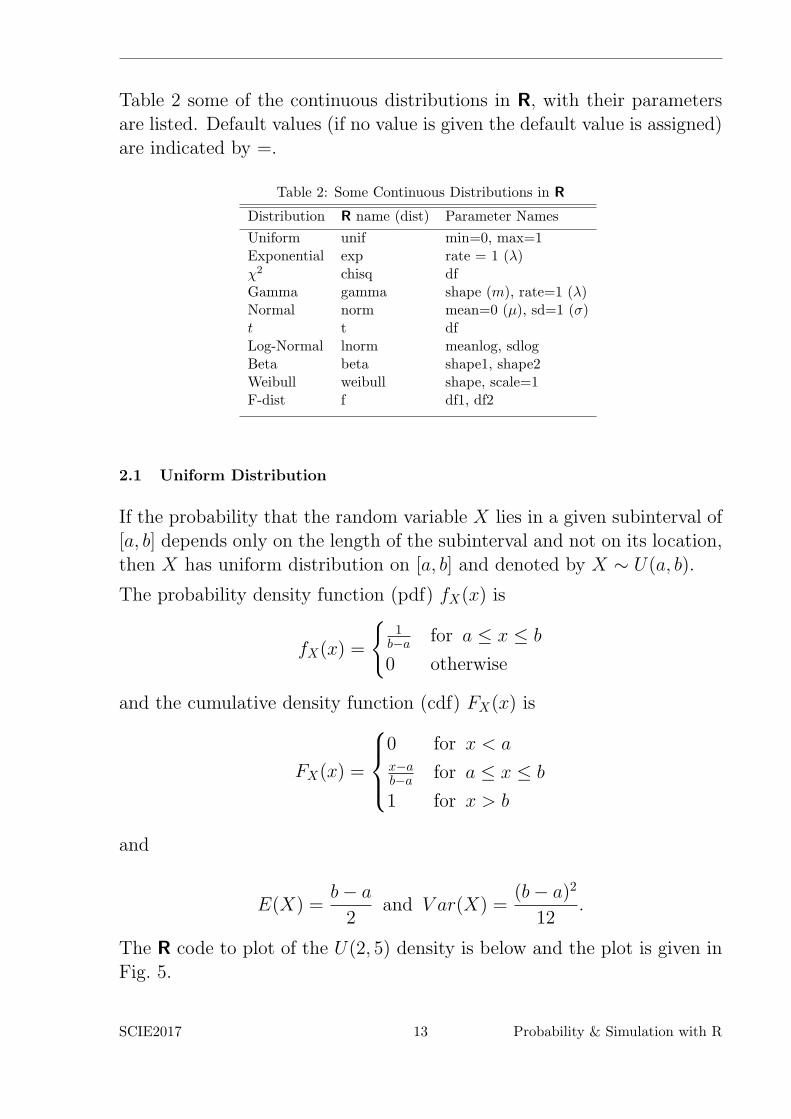
Table 2 some of the continuous distributions in R, with their parametersare listed. Default values (if no value is given the default value is assigned)are indicated by =.
Table 2: Some Continuous Distributions in R
Distribution R name (dist) Parameter Names
Uniform unif min=0, max=1Exponential exp rate = 1 (λ)χ2 chisq dfGamma gamma shape (m), rate=1 (λ)Normal norm mean=0 (µ), sd=1 (σ)t t dfLog-Normal lnorm meanlog, sdlogBeta beta shape1, shape2Weibull weibull shape, scale=1F-dist f df1, df2
2.1 Uniform Distribution
If the probability that the random variable X lies in a given subinterval of[a, b] depends only on the length of the subinterval and not on its location,then X has uniform distribution on [a, b] and denoted by X ∼ U(a, b).
The probability density function (pdf) fX(x) is
fX(x) =
{1
b−a for a ≤ x ≤ b
0 otherwise
and the cumulative density function (cdf) FX(x) is
FX(x) =
0 for x < ax−ab−a for a ≤ x ≤ b
1 for x > b
and
E(X) =b− a
2and V ar(X) =
(b− a)2
12.
The R code to plot of the U(2, 5) density is below and the plot is given inFig. 5.
SCIE2017 13 Probability & Simulation with R
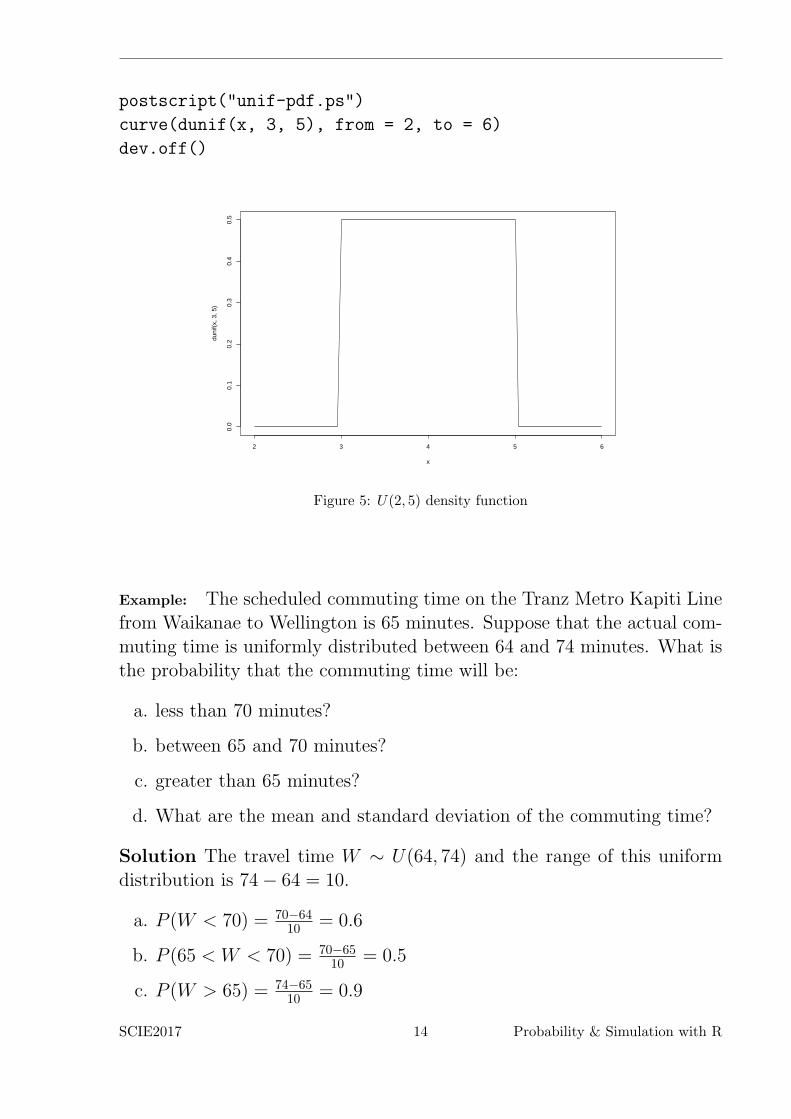
postscript("unif-pdf.ps")
curve(dunif(x, 3, 5), from = 2, to = 6)
dev.off()
2 3 4 5 6
0.0
0.1
0.2
0.3
0.4
0.5
x
duni
f(x,
3, 5
)
Figure 5: U(2, 5) density function
Example: The scheduled commuting time on the Tranz Metro Kapiti Linefrom Waikanae to Wellington is 65 minutes. Suppose that the actual com-muting time is uniformly distributed between 64 and 74 minutes. What isthe probability that the commuting time will be:
a. less than 70 minutes?
b. between 65 and 70 minutes?
c. greater than 65 minutes?
d. What are the mean and standard deviation of the commuting time?
Solution The travel time W ∼ U(64, 74) and the range of this uniformdistribution is 74− 64 = 10.
a. P (W < 70) = 70−6410 = 0.6
b. P (65 < W < 70) = 70−6510 = 0.5
c. P (W > 65) = 74−6510 = 0.9
SCIE2017 14 Probability & Simulation with R

d. E(W ) = 74+642 = 69 and SD =
((74−64)2
12
) 12
= 0.866025
We can solve this problem using R.
a.
> punif(70, 64, 74)
[1] 0.6
b.
> punif(70, 64, 74) - punif(65, 64, 74)
[1] 0.5
c.
> 1 - punif(65, 64, 74)
[1] 0.9
d.
(1) using an R function to exactly compute the mean value
exval_unif<- function(a, b)
{
m <- (a+b)/2
return (m)
}
print(exval_unif(64,74))
with output
[1] 69
(2) using an R function to exactly compute the standard deviation
sd_unif<- function(a, b)
{
sdu <- sqrt((b - a)^2/12)
return (sdu)
}
print(sd_unif(64,74))
SCIE2017 15 Probability & Simulation with R
with output
[1] 2.886751
(3) Generating U(64, 74) observations to estimate the mean
and standard deviation of the commuting time
> x <-runif(1000000, 64,74) #generated 1000000 U(64, 74) observations
> mean(x)
[1] 69.00091
> var(x)
[1] 8.347934
> sd(x)
[1] 2.887092
2.2 Lifetime Models
2.2.1 Exponential Distribution
A continuous random variable X has an exponential distribution with pa-rameter λ > 0, denoted by X ∼ exp(λ), if its pdf f(x) is given by
f(x) =
{λ e−λx forx ≥ 0
0 forx < 0
or equivalently if its cdf is given by
F (x) =
{1− e−λx forx ≥ 0
0 forx < 0
Also,
E(X) =1
λand V ar(X) =
1
λ2.
SCIE2017 16 Probability & Simulation with R
■ Note: The parameter λ of the exp(λ) is equal to thereciprocal of the expected value E(X) = 1
λ of X ∼ exp(λ).
For exp(λ) distribution, the failure rate is a constant, λ(x) = λ and theequipment does not age, i.e., the equipment failures are “at random”. This“non-aging” property of the exponential distribution is called the memory-less (or forgetfulness, or lack of memory) property. It says that, for s, t > 0
P (X > s+ t | X > s) = P (X > t),
i.e., given that the equipment has survived until age s, the probability tosurvive an additional time t is the same as for a new equipment. Theexp(λ) distribution is the only continuous distribution with this property.
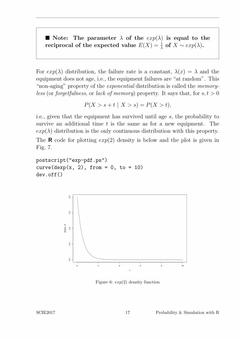
The R code for plotting exp(2) density is below and the plot is given inFig. 7.
postscript("exp-pdf.ps")
curve(dexp(x, 2), from = 0, to = 10)
dev.off()
0 2 4 6 8 10
0.0
0.5
1.0
1.5
2.0
x
dexp
(x, 2
)
Figure 6: exp(2) density function
SCIE2017 17 Probability & Simulation with R
Example: Suppose that the time T one spends in a bank is exponentiallydistributed with mean ten minutes, i.e., T ∼ exp(0.1).
(a) What is the probability that a customer will spend more than fifteenminutes in the bank?
P (T > 15) = e−15 λ = e−32 ≈ 0.223
> 1 - pexp(15, 0.1)
[1] 0.2231302
(b) What is the probability that a customer will spend more than fifteenminutes in the bank given that she is still in the bank after ten min-utes?
Due to the memoryless property of the exponential distribution
P (X > 10 + 5 | T > 10) = P (T > 5) = e−5 λ = e−12 = 0.6065307.
> 1 - pexp(5, 0.1)
[1] 0.6065307
Compare with
> (1 - pexp(15, 0.1))/(1 - pexp(10, 0.1))
[1] 0.6065307
2.3 Gamma Distribution
The exponential distribution is a continuous analogue of the geometricdistribution. The sum of independent geometric random variables hasa negative binomial distribution. The continuous analog of the negativebinomial distribution is the gamma distribution. Let X be the sum of mindependent exp(λ) random variables. Then X has a gamma distributionwith parameters λ and m, denoted by X ∼ gamma(λ,m). It can be shownthat X has the following characteristics, for m,λ > 0 and x ≥ 0
f(x) =1
Γ(m)λm xm−1 e−λ x,
SCIE2017 18 Probability & Simulation with R
andµ =
m
λand σ2 =
m
λ2.
This definition holds for any m > 0 not only for integer values. If m isan integer, the gamma distribution is known as the Erlang distribution oforder m.
■ In R the default order of the parameters of the gammadistribution is (m,λ) rather than (λ,m). The best is to specifyexplicitly each of them as shape = and rate =.
The following R code will produce some gamma densities
> curve(dgamma(x, shape = 0.5, rate = 2), from = 0, to = 4)
> curve(dgamma(x, shape = 1.5, rate = 2), from = 0, to = 4)
> curve(dgamma(x, shape = 3, rate = 2), from = 0, to = 4)
Example: Suppose that when a transistor of a certain type is subjected toan accelerated life test, the lifetime X (in weeks) has a gamma distributionwith mean of 40 and variance of 320. What is the probability that thetransistor will last between 8 and 40 weeks?
We need to determine the parameters of the gamma distribution of thelifetime X, i.e, to solve
m
λ= 40 and
m
λ2= 320
simultaneously for m and λ, which leads to m = 5 and λ = 18 . Thus
> pgamma(40, 5, 1/8) - pgamma(8, 5, 1/8)
[1] 0.5558469.
2.4 Sampling distributions
The following distributions are used in Statistics quite often because theyappear naturally when dealing with random samples.
SCIE2017 19 Probability & Simulation with R
2.4.1 Normal (or Gaussian) Distribution
The importance of the Normal (or Gaussian) distribution is due to theCentral Limit Theorem. This theorem tells us that the average of a suffi-ciently large iid sample is a normal random variable. A continuous randomvariable X has a Normal distribution with parameters µ and σ2, denotedby X ∼ N(µ, σ2), if its pdf is
f(x) =1√2πσ2
e−(x−µ)2
2σ2 for −∞ < x < ∞.
If µ = 0 and σ2 = 1 then the distribution is called standard normaldistribution, usually denoted by Z ∼ N(0, 1). If Z ∼ N(0, 1), thenX = σZ + µ ∼ N(µ, σ2).
The following R code will produce some normal densities
> curve(dnorm(x, mean = 0, sd = 1), from = -5, to = 5)
> curve(dnorm(x, mean = 1, sd = 1), from = -5, to = 5)
> curve(dnorm(x, mean = 2, sd = 1), from = -5, to = 5)
We can put all of these density in one plot
curve(dnorm(x, mean = 0, sd = 1), from = -4, to = 6)
curve(dnorm(x, mean = 1, sd = 1), add=T)
curve(dnorm(x, mean = 2, sd = 1), add=T)
We start by showing that the rnorm function works by generating an iidsample of N(0, 1) random variables and showing that their histogram lookslike the normal density.
postscript("out.ps")
z<-rnorm(10000)
par(las = 1) # identifies the way the axes are labelled (las = 1) means horizontal
hist(z, breaks = seq(-5, 5, 0.2), freq = F) # breaks gives the breakpoints
# of histogram cells
# freq = F means that probability densities are
# plotted (the hist has a total area of one)
phi <- function(x) exp(-x^2/2)/sqrt(2*pi)
x<- seq(-5, 5, 0.1)
lines(x,phi(x))
dev.off()
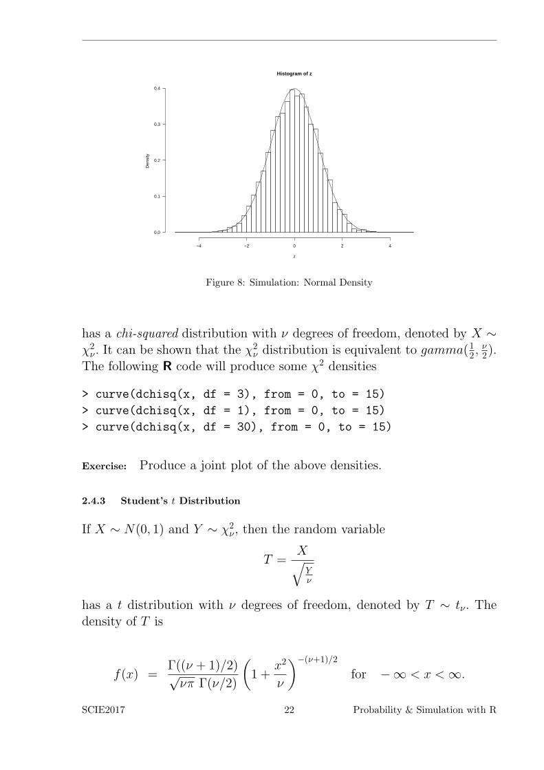
The result is stored in the file out.ps and output is given in Fig.8.
The sum of independent normals It is well known that if X ∼ N(µ1, σ21) and
Y ∼ N(µ2, σ22) are independent, then X + Y ∼ N(µ1 + µ2, σ
21 + σ2
2). Wewill verify this result experimentally using the rnorm function.
SCIE2017 20 Probability & Simulation with R

−4 −2 0 2 4 6
0.0
0.1
0.2
0.3
0.4
x
dnor
m(x
, mea
n =
0, s
d =
1)
Figure 7: Multiple densities in one plot
postscript("out.ps")
z1<-rnorm(10000, mean = 1, sd = 1)
z2<-rnorm(10000, mean = 1, sd = 2)
z <- z1 + z2
mean(z)
var(z)
par(las = 1) # set the axis labeling style
hist(z, breaks = seq(-10, 14, 0.2), freq = F)
phi <- function(x) exp(-(x-2)^2/10)/sqrt(10*pi)
x<- seq(-10, 14, 0.1)
lines(x,phi(x))
dev.off()
The result is stored in the file out.ps and output is given in Fig.9.
The plot shows that the histogram is very close to the theoretical density,which supports the theory.
2.4.2 χ2 Distribution
Suppose Z1, Z2, . . . , Zν are iid N(0, 1) random variables. Then
X = Z1 + Z2 + . . .+ Zν
SCIE2017 21 Probability & Simulation with R
Histogram of z
z
Den
sity
−4 −2 0 2 4
0.0
0.1
0.2
0.3
0.4
Figure 8: Simulation: Normal Density
has a chi-squared distribution with ν degrees of freedom, denoted by X ∼χ2ν. It can be shown that the χ2
ν distribution is equivalent to gamma(12 ,ν2).
The following R code will produce some χ2 densities
> curve(dchisq(x, df = 3), from = 0, to = 15)
> curve(dchisq(x, df = 1), from = 0, to = 15)
> curve(dchisq(x, df = 30), from = 0, to = 15)
Exercise: Produce a joint plot of the above densities.
2.4.3 Student’s t Distribution
If X ∼ N(0, 1) and Y ∼ χ2ν, then the random variable
T =X√Yν
has a t distribution with ν degrees of freedom, denoted by T ∼ tν. Thedensity of T is
f(x) =Γ((ν + 1)/2)√νπ Γ(ν/2)
(1 +
x2
ν
)−(ν+1)/2
for −∞ < x < ∞.
SCIE2017 22 Probability & Simulation with R

Histogram of z
z
Den
sity
−10 −5 0 5 10
0.00
0.05
0.10
0.15
Figure 9: Simulation: Sum of Independent Normals
The density of T ∼ tν is symmetric with shape similar to N(0, 1), butwith fatter (i.e., more probability at large distances from 0) tails. Whenthe degree of freedom ν tends to ∞, the density of T ∼ tν approachesthe density of Z ∼ N(0, 1). The following R code will produce some tνdensities
> curve(dt(x, df = 3), from = 0, to = 15)
> curve(dt(x, df = 1), from = 0, to = 15)
> curve(dt(x, df = 30), from = 0, to = 15)
Exercise: Produce a joint plot of the above densities.
Exercise: Use simulation to show that when the degrees of freedom ν tendsto ∞, the density of T ∼ tν approaches the density of Z ∼ N(0, 1).
SCIE2017 23 Probability & Simulation with R
3 Random Generators
We can not generate truly random numbers on a computer. Instead wegenerate pseudo-random numbers, which have the appearance of randomnumbers but in fact they are completely deterministic (i.e., can be repro-duced).
3.1 Congruential Random Generators
Congruential random number generators were the first reasonable class ofpseudo-random numbers generators. They produce pseudo-random integernumbers.
Consider an initial number X0 ∈ {0, 1, 2, . . . ,m−1} (usually called a seed)and two big numbers a and c. We define a sequence of numbers Xn ∈{0, 1, 2, . . . ,m− 1}, n = 0, 1, 2, . . . , by
Xn+1 = (a Xn + c) mod m.
(mod m) means modulo m operation, which finds the integer remainder (inour case Xn+1) of the division of a given number (in our case (a Xn + c))by m.
Example: If m = 10, a = 103 and c = 17, then for X0 = 2, we have
X1 = 223 = 3 mod 10
X2 = 326 = 6 mod 10
X3 = 635 = 5 mod 10...
...
Clearly the sequence produced by the congruential random number gener-ator will eventually cycle and thus, because there are at most m possiblevalues {0, 1, . . . ,m− 1}, the maximum cycle length is m. An example of agood congruential random number generator (with a long cycle length) ism = 232, a = 1664525 and c = 1013904223.
3.2 Seeding
The initial number X0 is called the seed (this is the number the generatorstarts from). If a, c, m and X0 are known then any integer sequence can be
SCIE2017 24 Probability & Simulation with R
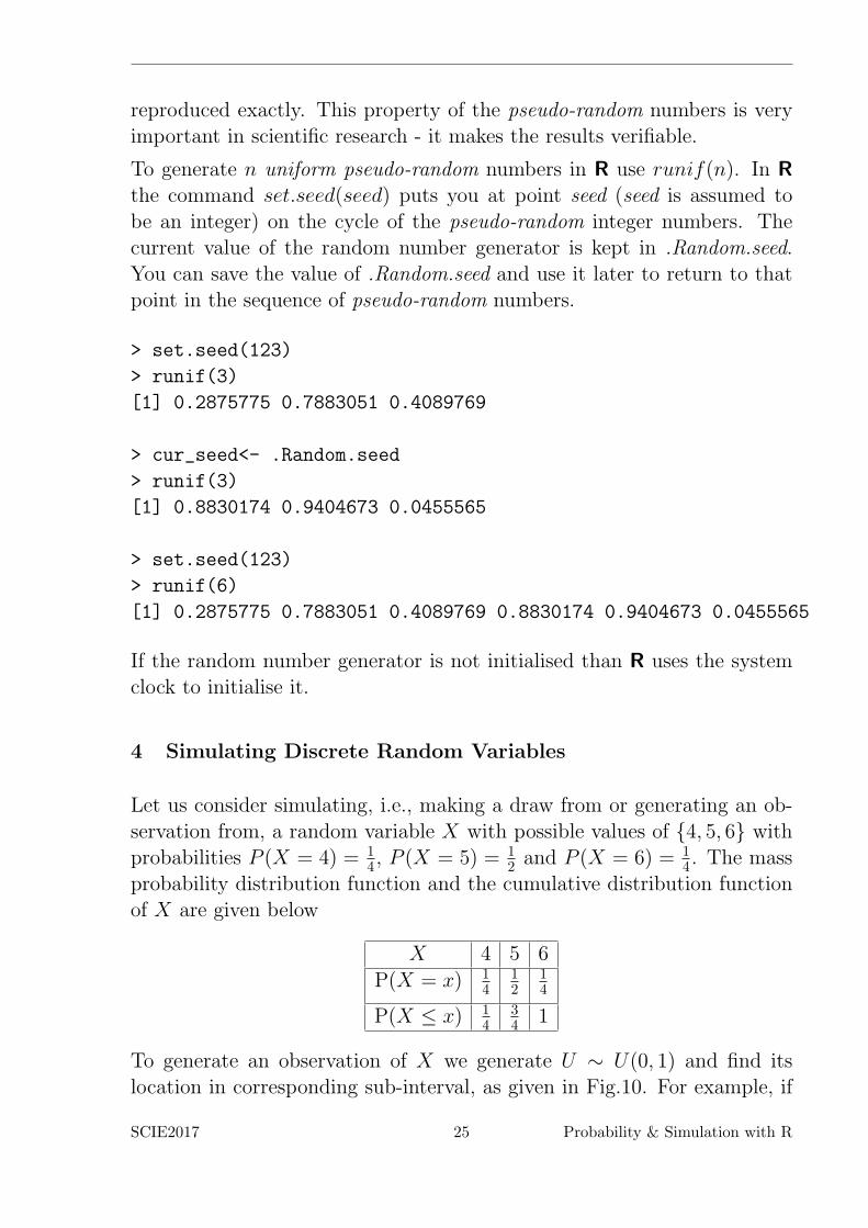
reproduced exactly. This property of the pseudo-random numbers is veryimportant in scientific research - it makes the results verifiable.
To generate n uniform pseudo-random numbers in R use runif(n). In Rthe command set.seed(seed) puts you at point seed (seed is assumed tobe an integer) on the cycle of the pseudo-random integer numbers. Thecurrent value of the random number generator is kept in .Random.seed.You can save the value of .Random.seed and use it later to return to thatpoint in the sequence of pseudo-random numbers.
> set.seed(123)
> runif(3)
[1] 0.2875775 0.7883051 0.4089769
> cur_seed<- .Random.seed
> runif(3)
[1] 0.8830174 0.9404673 0.0455565
> set.seed(123)
> runif(6)
[1] 0.2875775 0.7883051 0.4089769 0.8830174 0.9404673 0.0455565
If the random number generator is not initialised than R uses the systemclock to initialise it.
4 Simulating Discrete Random Variables
Let us consider simulating, i.e., making a draw from or generating an ob-servation from, a random variable X with possible values of {4, 5, 6} withprobabilities P (X = 4) = 1
4 , P (X = 5) = 12 and P (X = 6) = 1
4 . The massprobability distribution function and the cumulative distribution functionof X are given below
X 4 5 6
P(X = x) 14
12
14
P(X ≤ x) 14
34 1
To generate an observation of X we generate U ∼ U(0, 1) and find itslocation in corresponding sub-interval, as given in Fig.10. For example, if
SCIE2017 25 Probability & Simulation with R
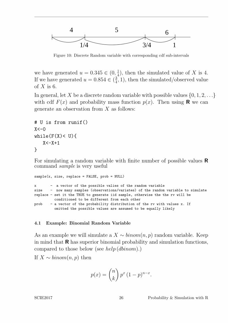
1/4 3/4 1
4 5 6
Figure 10: Discrete Random variable with corresponding cdf sub-intervals
we have generated u = 0.345 ∈ (0, 14), then the simulated value of X is 4.If we have generated u = 0.854 ∈ (34 , 1), then the simulated/observed valueof X is 6.
In general, letX be a discrete random variable with possible values {0, 1, 2, . . .}with cdf F (x) and probability mass function p(x). Then using R we cangenerate an observation from X as follows:
# U is from runif()
X<-0
while(F(X)< U){
X<-X+1
}
For simulating a random variable with finite number of possible values Rcommand sample is very useful
sample(x, size, replace = FALSE, prob = NULL)
x - a vector of the possible valies of the random variable
size - now many samples (observations/variates) of the random variable to simulate
replace - set it the TRUE to generate iid sample, otherwise the the rv will be
conditioned to be different from each other
prob - a vector of the probability distribution of the rv with values x. If
omitted the possible values are assumed to be equally likely
4.1 Example: Binomial Random Variable
As an example we will simulate a X ∼ binom(n, p) random variable. Keepin mind that R has superior binomial probability and simulation functions,compared to those below (see help (dbinom).)
If X ∼ binom(n, p) then
p(x) =
(n
k
)px (1− p)n−x.
SCIE2017 26 Probability & Simulation with R
Exercise: Simulate 5 observations from binom(12, 0.3).
4.2 Sequence of independent trials
For random variables that are defined using independent Bernoulli trials(such as binomial, geometric, and negative binomial) the following methodof generating them is very useful.
# B is Bernoulli(p)
#given U is a draw from U(0, 1)
if (U < p) {B <- 1} else {B <- 0}
(a) Then given n and p, the R code to generate a binomial(n, p) randomvariable X is
X <- 0
for (i in 1:n){ # n is the number of trials
U <- runif(1)
if (U < p) X <- X + 1 # the outcome is a success
}
(b) Alternatively, because R assigns 1 to TRUE and 0 to FALSE, givenn and p
X <- sum(runif(n) < p)
will generate a X ∼ binomial(n, p).
4.3 Example: Geometric Random Variable
Given p, (in the example p = 0.1) to generate Y ∼ geom(p), we can use
p = 0.1
Y <- 0
success <- FALSE
while (!success){
U <- runif(1)
if (U < p) {
success <- TRUE
} else {
SCIE2017 27 Probability & Simulation with R
Y <- Y + 1
}
}
4.4 Example: Negative Binomial Random Variable
Exercise Write a fragment of R code to generate an observation fromZ ∼ nbinom(r, p). (Hint: Use the relationship betweem geom(p) andnbinom(r, p).)
5 Simulating Continuous Random Variables
5.1 Inverse Transformation Method (ITM)
Suppose U ∼ U(0, 1), i.e.,
P (U ≤ u) = u,
and we want to simulate a continuous random variable X with cdf FX(x).
Set Y = F−1X (U), then
FY (y) = P (Y ≤ y) = P (F−1X (U) ≤ y)
= P (U ≤ FX(y)) = FX(y)
Therefore Y has the same distribution as X. If we can simulate an ob-servation from U ∼ U(0, 1) then we can simulate any continuous X withknown inverse cdf F−1
X (x). This approach is called inverse transfor-mation method (ITM). It is the continuous analogue of the method forsimulating discrete random variables given in Section 4.
Example: Exponential distribution A continuous random variable X has anexponential distribution with parameter λ > 0, X ∼ exp(λ), if its pdf isgiven by
f(x)
{λ e−λx forx ≥ 0
0 forx < 0
or equivalently if its cdf is given by
SCIE2017 28 Probability & Simulation with R
F (x)
{1− e−λx forx ≥ 0
0 forx < 0.
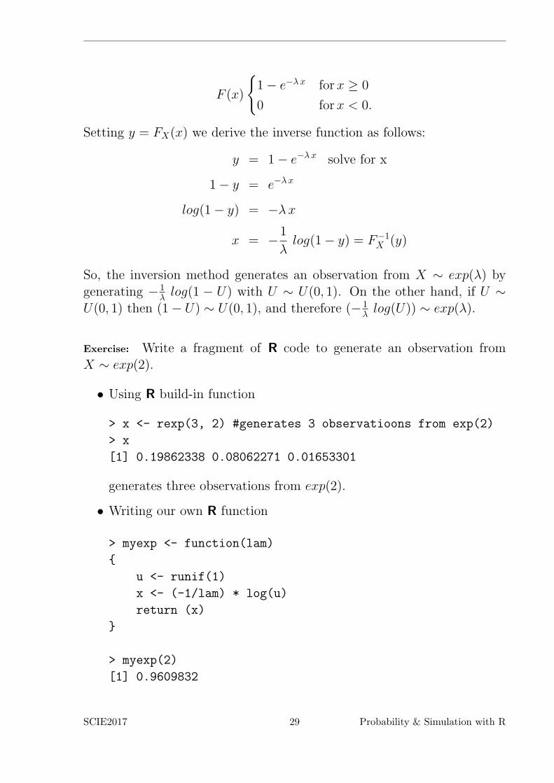
Setting y = FX(x) we derive the inverse function as follows:
y = 1− e−λx solve for x
1− y = e−λx
log(1− y) = −λx
x = −1
λlog(1− y) = F−1
X (y)
So, the inversion method generates an observation from X ∼ exp(λ) bygenerating − 1
λ log(1 − U) with U ∼ U(0, 1). On the other hand, if U ∼U(0, 1) then (1− U) ∼ U(0, 1), and therefore (− 1
λ log(U)) ∼ exp(λ).
Exercise: Write a fragment of R code to generate an observation fromX ∼ exp(2).
• Using R build-in function
> x <- rexp(3, 2) #generates 3 observatioons from exp(2)
> x
[1] 0.19862338 0.08062271 0.01653301
generates three observations from exp(2).
• Writing our own R function
> myexp <- function(lam)
{
u <- runif(1)
x <- (-1/lam) * log(u)
return (x)
}
> myexp(2)
[1] 0.9609832
SCIE2017 29 Probability & Simulation with R
Exercise: Write a fragment of R code to generate an observation from X,which has an Erlang distribution of order 4 with mean E(X) = 4, whichis a sum of four iid exp(1).
SCIE2017 30 Probability & Simulation with R
6 Practice Problems with R
6.1 Monty Hall Game
• Suppose you are on a game show, such that you can win a car if youguess its location. You are given the choice of three doors:
(a) the car is behind one of the doors, and goats are behind the othertwo doors;
(b) you pick a door, say No. 1;
(c) the host, who knows what is behind the doors, opens a “goat”door;
(d) then the host asks you ”Do you want to switch your door choiceand pick door No. 2?”
Is it to your advantage to switch your door choice? The rules of thegame are as follows:
(a) You make an initial guess
(b) The master opens one of the “goat” doors
(c) You have a chance to revise your initial guess before making yourfinal choice:
– Strategy A: stick with your initial guess
– Strategy B: switch to another door
Simulate this game. Which strategy (A or B) do you prefer? What isthe criterion for your decision?
#no switch strategy
#number of plays
N=100000
# counter for wins
s = 0
for (i in 1:N){
#select the door with the car
DC = sample(c(1,2,3), 1, replace = FALSE, prob=c(1/3,1/3,1/3))
# select the door of the player choice
C1 = sample(c(1,2,3), 1, replace = FALSE, prob=c(1/3,1/3,1/3))
#the strategy is "no switch", if the two doors are the same (DC==C1), then the
#player wins
if(DC == C1) rez <-1
else rez <- 0
s = s+rez
}
#computing the probability of win
SCIE2017 31 Probability & Simulation with R
PW = s/N
print(PW)
#switch strategy
s = 0
for (i in 1:N){
DC = sample(c(1,2,3), 1, replace = FALSE, prob=c(1/3,1/3,1/3))
C1 = sample(c(1,2,3), 1, replace = FALSE, prob=c(1/3,1/3,1/3))
#the strategy is "switch", if the two doors are the same (DC!=C1), after switch
#he player wins
if(DC!= C1) rez = 1
else rez = 0
s = s+rez
}
PW1 = s/N
cat("ProbWin (Switch) = ", PW1, " ","ProbWin (No Switch) = ", PW, "\n")
My output is
OUTPUT=========
[1] 0.33223
ProbWin (Switch) = 0.6694 ProbWin (No Switch) = 0.33223
• How does this problem change if Monty Hall does not know where thecar is located? We must decide what it means if Monty should happento open the door with the car behind by accident. So we interpret thisto mean that if the car is revealed then the game is over (no winningor losing) and the next round of the game starts.
Which strategy (A or B) do you prefer?
#no switch strategy
#number of plays
N=100000
# counter for wins
s = 0
for (i in 1:N){
#select the door with the car
DC = sample(c(1,2,3), 1, replace = FALSE, prob=c(1/3,1/3,1/3))
# select the door of the player choice
C1 = sample(c(1,2,3), 1, replace = FALSE, prob=c(1/3,1/3,1/3))
# select the door of the host choice
H1 <-sample(c(1,2,3), 1, replace = FALSE, prob=c(1/3,1/3,1/3))
SCIE2017 32 Probability & Simulation with R
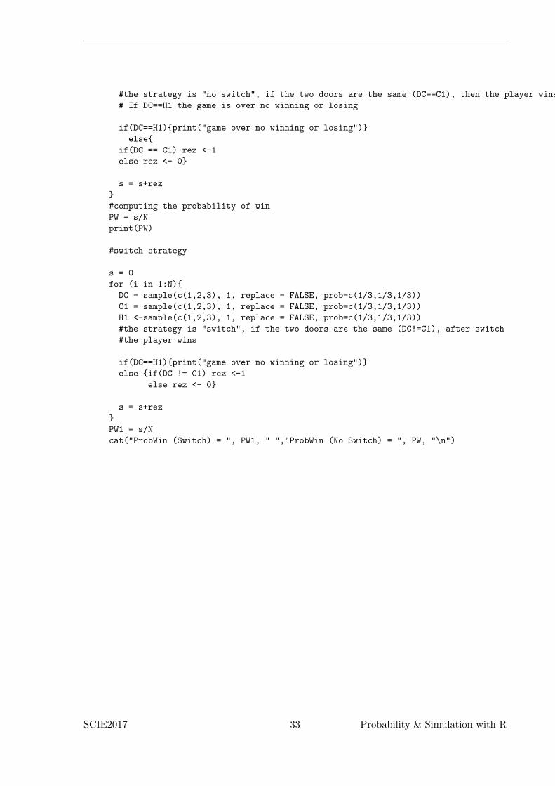
#the strategy is "no switch", if the two doors are the same (DC==C1), then the player wins
# If DC==H1 the game is over no winning or losing
if(DC==H1){print("game over no winning or losing")}
else{
if(DC == C1) rez <-1
else rez <- 0}
s = s+rez
}
#computing the probability of win
PW = s/N
print(PW)
#switch strategy
s = 0
for (i in 1:N){
DC = sample(c(1,2,3), 1, replace = FALSE, prob=c(1/3,1/3,1/3))
C1 = sample(c(1,2,3), 1, replace = FALSE, prob=c(1/3,1/3,1/3))
H1 <-sample(c(1,2,3), 1, replace = FALSE, prob=c(1/3,1/3,1/3))
#the strategy is "switch", if the two doors are the same (DC!=C1), after switch
#the player wins
if(DC==H1){print("game over no winning or losing")}
else {if(DC != C1) rez <-1
else rez <- 0}
s = s+rez
}
PW1 = s/N
cat("ProbWin (Switch) = ", PW1, " ","ProbWin (No Switch) = ", PW, "\n")
SCIE2017 33 Probability & Simulation with R
6.2 Project Selection (OPTIONAL)
Tazer Corp., a pharmaceutical company, is beginning to search for a newbreakthrough drug. The following five potential research and developmentprojects have been identified for attempting to develop such a drug:
project Up: Develop a more effective antidepressant that does not causeserious mood swings;
project Stable: Develop a drug that addresses a manic depression;
project Choice: Develop a less intrusive a birth control method for women;
project Hope: Develop a vaccine to prevent HIV infection;
project Release: Develop a more effective drug to lower blood pressure.
Tazer management has concluded that the company can not devote enoughmoney to R&D to undertake all of these projects. Only $1200(millions) isavailable, which is be enough for two or three projects.
The data for the Tazer project selection project are given in table 3.
RD Investment Revenue (if successful)
Project ($milions) Success Rate Mean Standard Deviation
Up 400 0.50 1400 400Stable 300 0.35 1200 400Choice 600 0.35 2200 600Hope 500 0.20 3000 900Release 200 0.45 600 200
Table 3: Data for the Tazer project selection project
If a project is successful, it is quite uncertain how much revenue the drugwould generate. The estimate of the revenue (in millions of dollars) is thatit has a normal distribution with the mean and the standard deviationgiven in the last two columns of table 3.
Tazer management wants to determine
(a) which of these projects should be undertaken to maximise the expectedtotal profit from the resulting revenues (if any);
(b) to have a reasonable high probability of achieving a satisfactory totalprofit (at least $100 million).
Specify the best decision for the Tazer management under each of theobjectives.
SCIE2017 34 Probability & Simulation with R
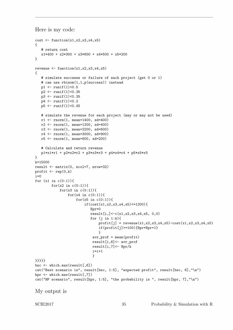
Here is my code:
cost <- function(x1,x2,x3,x4,x5)
{
# return cost
x1*400 + x2*300 + x3*600 + x4*500 + x5*200
}
revenue <- function(x1,x2,x3,x4,x5)
{
# simulate succeses or failure of each project (get 0 or 1)
# can use rbinom(1,1,p(success)) instead
p1 <- runif(1)<0.5
p2 <- runif(1)<0.35
p3 <- runif(1)<0.35
p4 <- runif(1)<0.2
p5 <- runif(1)<0.45
# simulate the revenue for each project (may or may not be used)
r1 <- rnorm(1, mean=1400, sd=400)
r2 <- rnorm(1, mean=1200, sd=400)
r3 <- rnorm(1, mean=2200, sd=600)
r4 <- rnorm(1, mean=3000, sd=900)
r5 <- rnorm(1, mean=600, sd=200)
# Calculate and return revenue
p1*x1*r1 + p2*x2*r2 + p3*x3*r3 + p4*x4*r4 + p5*x5*r5
}
k=15000
result <- matrix(0, ncol=7, nrow=32)
profit <- rep(0,k)
i=0
for (x1 in c(0:1)){
for(x2 in c(0:1)){
for(x3 in c(0:1)){
for(x4 in c(0:1)){
for(x5 in c(0:1)){
if(cost(x1,x2,x3,x4,x5)<=1200){
Npr=0
result[i,]<-c(x1,x2,x3,x4,x5, 0,0)
for (j in 1:k){
profit[j] = revenue(x1,x2,x3,x4,x5)-cost(x1,x2,x3,x4,x5)
if(profit[j]>=100){Npr=Npr+1}
}
avr_prof = mean(profit)
result[i,6]<- avr_prof
result[i,7]<- Npr/k
i=i+1
}
}}}}}
bsc <- which.max(result[,6])
cat("Best scenario is", result[bsc, 1:5], "expected profit", result[bsc, 6],"\n")
hpr <- which.max(result[,7])
cat("HP scenario", result[hpr, 1:5], "the probability is ", result[hpr, 7],"\n")
My output is
SCIE2017 35 Probability & Simulation with R
> source("proj_selection.r")
Best scenario is 1 1 0 1 0 expected profit 538.2499
HP scenario 1 1 0 0 0 the probability is 0.6230667
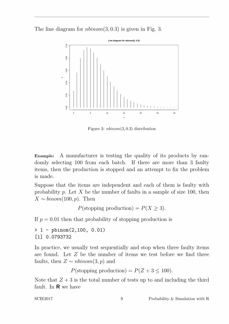
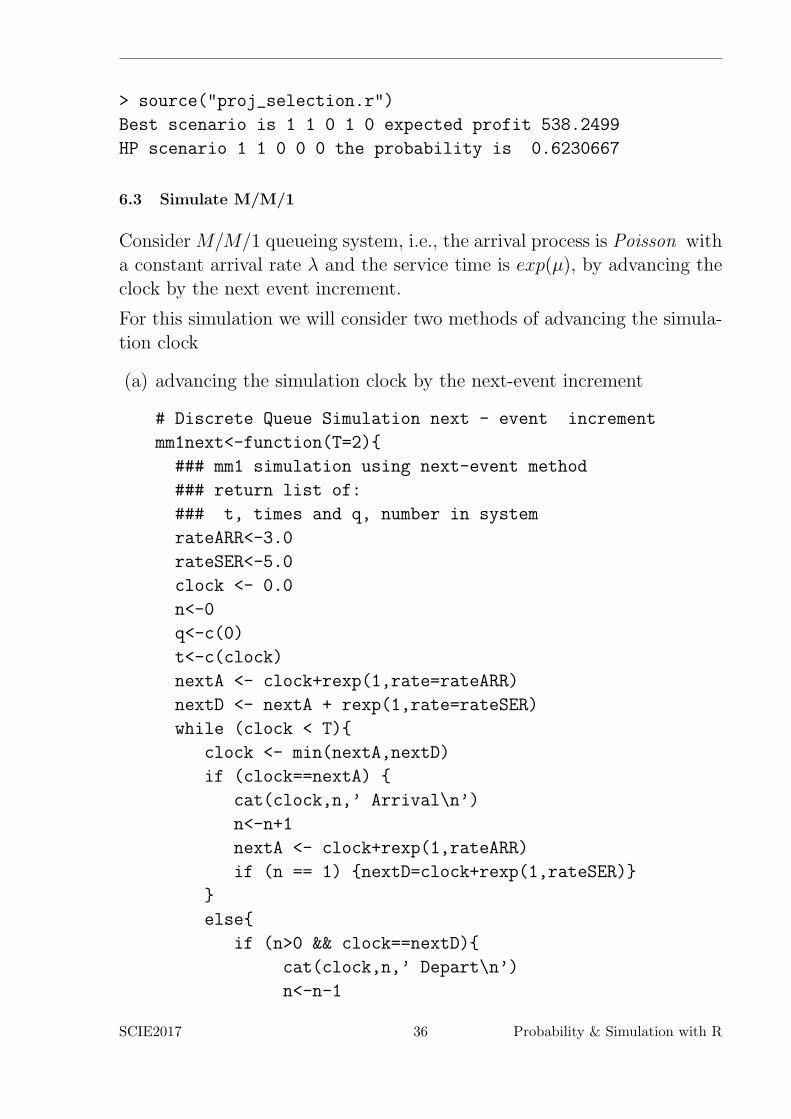
6.3 Simulate M/M/1
Consider M/M/1 queueing system, i.e., the arrival process is Poisson witha constant arrival rate λ and the service time is exp(µ), by advancing theclock by the next event increment.
For this simulation we will consider two methods of advancing the simula-tion clock
(a) advancing the simulation clock by the next-event increment
# Discrete Queue Simulation next - event increment
mm1next<-function(T=2){
### mm1 simulation using next-event method
### return list of:
### t, times and q, number in system
rateARR<-3.0
rateSER<-5.0
clock <- 0.0
n<-0
q<-c(0)
t<-c(clock)
nextA <- clock+rexp(1,rate=rateARR)
nextD <- nextA + rexp(1,rate=rateSER)
while (clock < T){
clock <- min(nextA,nextD)
if (clock==nextA) {
cat(clock,n,’ Arrival\n’)
n<-n+1
nextA <- clock+rexp(1,rateARR)
if (n == 1) {nextD=clock+rexp(1,rateSER)}
}
else{
if (n>0 && clock==nextD){
cat(clock,n,’ Depart\n’)
n<-n-1
SCIE2017 36 Probability & Simulation with R
if (n >=1) nextD<-clock+rexp(1,rateSER)
else nextD <- 99999
}
else cat("Error: ",clock,n,nextA,nextD,’\n’)
}
q<-append(q,n)
t<-append(t,clock)
}
return(list(t=t,q=q))
}
set.seed(34543)
reslt <- mm1next(20.0)
postscript("mm1_event.ps")
plot(reslt$t,reslt$q, type="s")
dev.off()
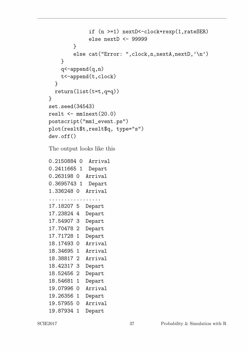
The output looks like this
0.2150884 0 Arrival
0.2411665 1 Depart
0.263198 0 Arrival
0.3695743 1 Depart
1.336248 0 Arrival
.................
17.18207 5 Depart
17.23824 4 Depart
17.54907 3 Depart
17.70478 2 Depart
17.71728 1 Depart
18.17493 0 Arrival
18.34695 1 Arrival
18.38817 2 Arrival
18.42317 3 Depart
18.52456 2 Depart
18.54681 1 Depart
19.07996 0 Arrival
19.26356 1 Depart
19.57955 0 Arrival
19.87934 1 Depart
SCIE2017 37 Probability & Simulation with R
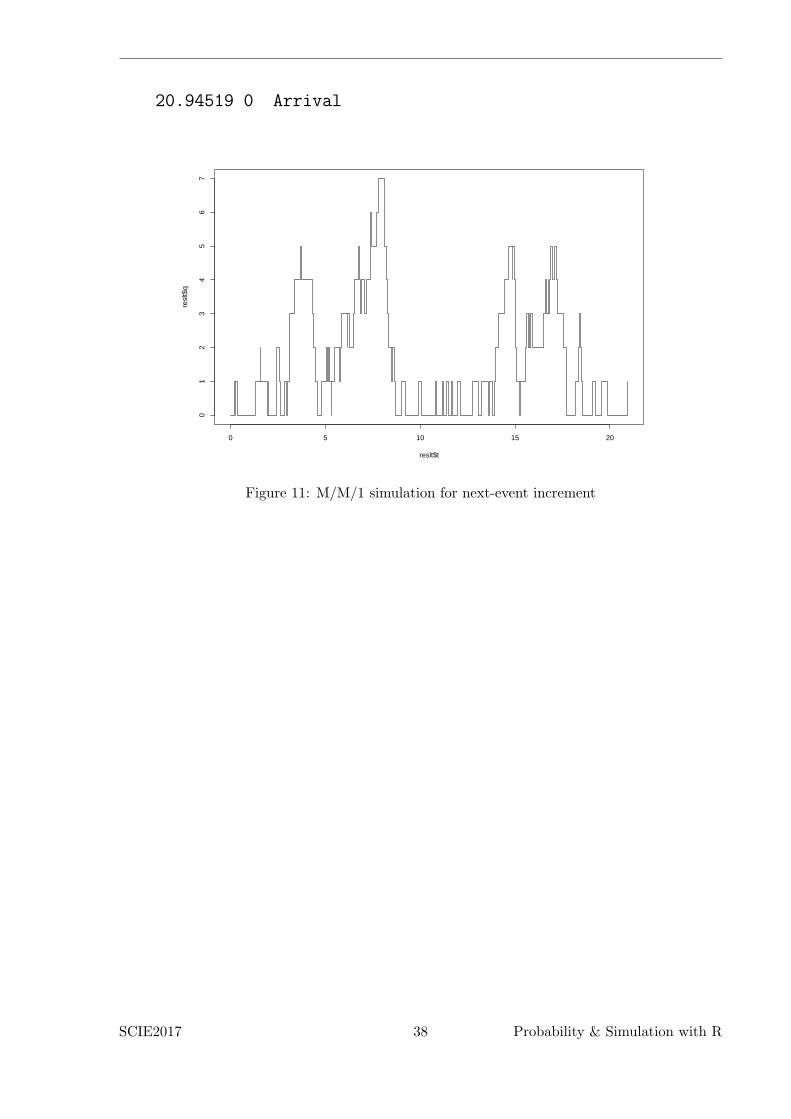
20.94519 0 Arrival
0 5 10 15 20
01
23
45
67
reslt$t
resl
t$q
Figure 11: M/M/1 simulation for next-event increment
SCIE2017 38 Probability & Simulation with R
7 Practice Problems
QUESTION 2 is OPTIONAL
1 Michael Wise operates a newsstand at a busy intersection downtown.Demand for the Sunday Times averages 300 copies with a standard devia-tion of 50 copies (assume a normal distriibution). Here are Michael’s costfigures:
• Michael pays $0.75 per copy delivered;
• Michael sells it for $1.25 per copy;
• Any paper left over at the end of the day are recycled with no monetaryreturn.
• Suppose Michael buys 350 copies for his newsstand each Sunday morn-ing. What would be Michael’s mean profit from selling the SundayTimes? What is the probability that Michael will make at least $0profit?
• Consider orders of {225, 250, 275, 300, 325, 350}. Which order quan-tity maximises Michael’s profit? What is the profit trend for these 6orders?
• Find the order quantity that maximises Michael’s profit. Use the aboveprofit trend to specify the range of reasonable orders.
sim078b
2 Hillier and Lierberman 20.1-3: Jessica Williams, manager of KitchenAppliances for the Midtown Department Store, feels that her inventorylevels of stoves have been running higher than necessary. Before revisingthe inventory policy for stoves, she records the number sold each day overa period of 25 days, as summarised below:
Number sold 2 3 4 5 6
Number of days 4 7 8 5 1
for performing a simulation
(a) Use the data to estimate the probability distribution of daily sales.
SCIE2017 39 Probability & Simulation with R
(b) Calculate the mean of the distribution obtained in part (a).
(c) Describe how uniform random numbers can be used to simulate dailysales.
(d) Use the uniform random numbres 0.4476, 0.9713, and 0.0629 to sim-ulate daily sales over 3 days. Compare the average with the meanobtained in part (b).
(e) Write aR simulation model of the daily sales. Perform 300 replicationsand obtain the average of the sales over the 300 simulated days.
sim096a
SCIE2017 40 Probability & Simulation with R
School of Mathematics, Statistics and Operation Research
Te Kura Matai Tatauranga, Rangahau Punaha
Feedback for Lab Guide — Probability & Simulation with R
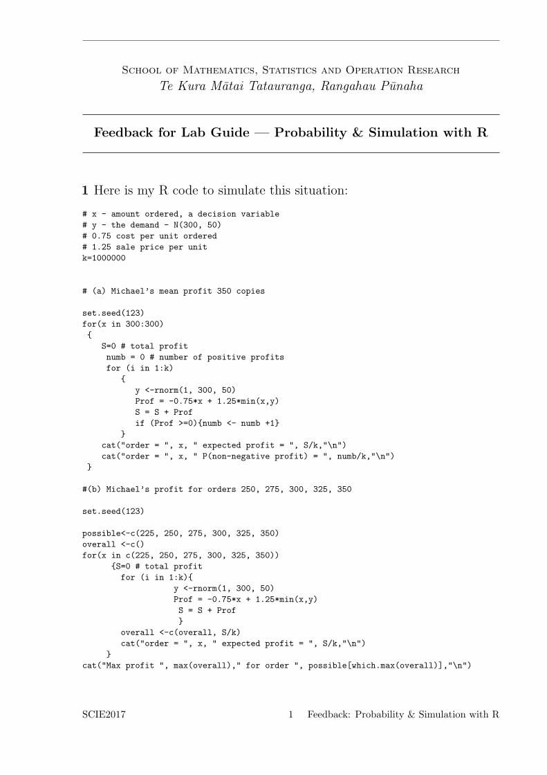
1 Here is my R code to simulate this situation:
# x - amount ordered, a decision variable
# y - the demand - N(300, 50)
# 0.75 cost per unit ordered
# 1.25 sale price per unit
k=1000000
# (a) Michael’s mean profit 350 copies
set.seed(123)
for(x in 300:300)
{
S=0 # total profit
numb = 0 # number of positive profits
for (i in 1:k)
{
y <-rnorm(1, 300, 50)
Prof = -0.75*x + 1.25*min(x,y)
S = S + Prof
if (Prof >=0){numb <- numb +1}
}
cat("order = ", x, " expected profit = ", S/k,"\n")
cat("order = ", x, " P(non-negative profit) = ", numb/k,"\n")
}
#(b) Michael’s profit for orders 250, 275, 300, 325, 350
set.seed(123)
possible<-c(225, 250, 275, 300, 325, 350)
overall <-c()
for(x in c(225, 250, 275, 300, 325, 350))
{S=0 # total profit
for (i in 1:k){
y <-rnorm(1, 300, 50)
Prof = -0.75*x + 1.25*min(x,y)
S = S + Prof
}
overall <-c(overall, S/k)
cat("order = ", x, " expected profit = ", S/k,"\n")
}
cat("Max profit ", max(overall)," for order ", possible[which.max(overall)],"\n")
SCIE2017 1 Feedback: Probability & Simulation with R
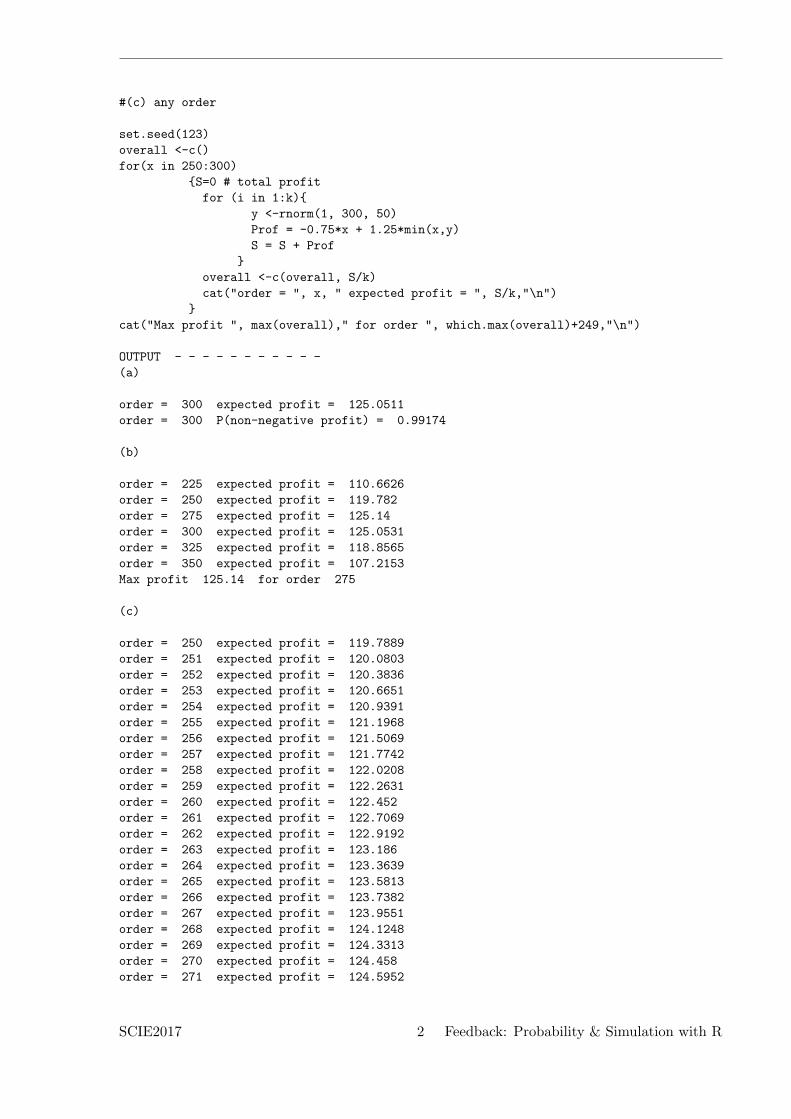
#(c) any order
set.seed(123)
overall <-c()
for(x in 250:300)
{S=0 # total profit
for (i in 1:k){
y <-rnorm(1, 300, 50)
Prof = -0.75*x + 1.25*min(x,y)
S = S + Prof
}
overall <-c(overall, S/k)
cat("order = ", x, " expected profit = ", S/k,"\n")
}
cat("Max profit ", max(overall)," for order ", which.max(overall)+249,"\n")
OUTPUT - - - - - - - - - - -
(a)
order = 300 expected profit = 125.0511
order = 300 P(non-negative profit) = 0.99174
(b)
order = 225 expected profit = 110.6626
order = 250 expected profit = 119.782
order = 275 expected profit = 125.14
order = 300 expected profit = 125.0531
order = 325 expected profit = 118.8565
order = 350 expected profit = 107.2153
Max profit 125.14 for order 275
(c)
order = 250 expected profit = 119.7889
order = 251 expected profit = 120.0803
order = 252 expected profit = 120.3836
order = 253 expected profit = 120.6651
order = 254 expected profit = 120.9391
order = 255 expected profit = 121.1968
order = 256 expected profit = 121.5069
order = 257 expected profit = 121.7742
order = 258 expected profit = 122.0208
order = 259 expected profit = 122.2631
order = 260 expected profit = 122.452
order = 261 expected profit = 122.7069
order = 262 expected profit = 122.9192
order = 263 expected profit = 123.186
order = 264 expected profit = 123.3639
order = 265 expected profit = 123.5813
order = 266 expected profit = 123.7382
order = 267 expected profit = 123.9551
order = 268 expected profit = 124.1248
order = 269 expected profit = 124.3313
order = 270 expected profit = 124.458
order = 271 expected profit = 124.5952
SCIE2017 2 Feedback: Probability & Simulation with R
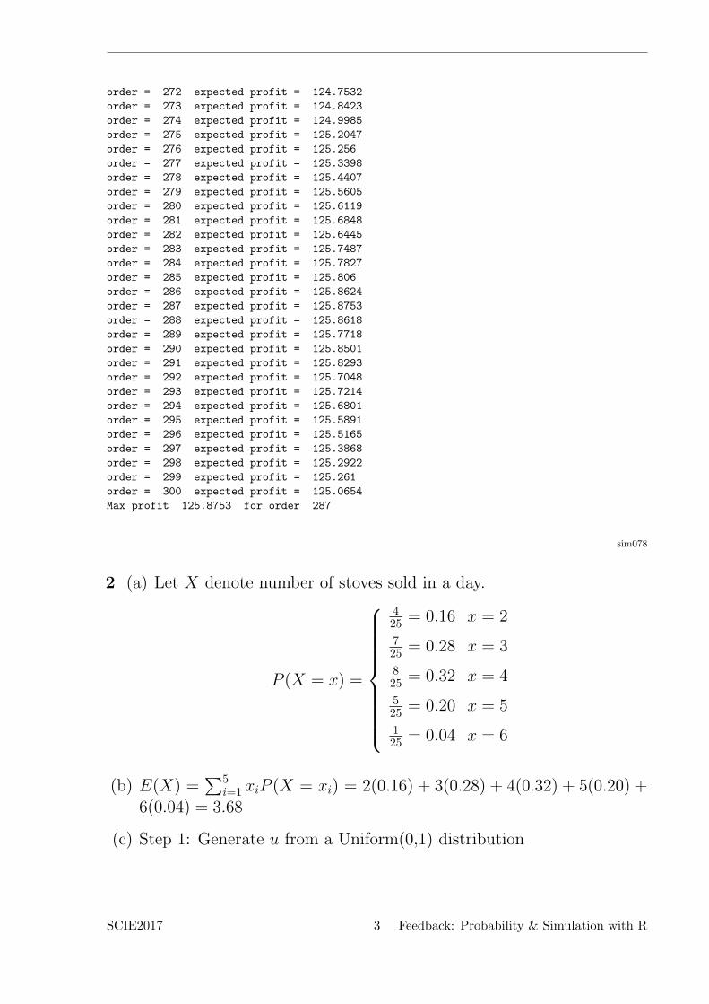
order = 272 expected profit = 124.7532
order = 273 expected profit = 124.8423
order = 274 expected profit = 124.9985
order = 275 expected profit = 125.2047
order = 276 expected profit = 125.256
order = 277 expected profit = 125.3398
order = 278 expected profit = 125.4407
order = 279 expected profit = 125.5605
order = 280 expected profit = 125.6119
order = 281 expected profit = 125.6848
order = 282 expected profit = 125.6445
order = 283 expected profit = 125.7487
order = 284 expected profit = 125.7827
order = 285 expected profit = 125.806
order = 286 expected profit = 125.8624
order = 287 expected profit = 125.8753
order = 288 expected profit = 125.8618
order = 289 expected profit = 125.7718
order = 290 expected profit = 125.8501
order = 291 expected profit = 125.8293
order = 292 expected profit = 125.7048
order = 293 expected profit = 125.7214
order = 294 expected profit = 125.6801
order = 295 expected profit = 125.5891
order = 296 expected profit = 125.5165
order = 297 expected profit = 125.3868
order = 298 expected profit = 125.2922
order = 299 expected profit = 125.261
order = 300 expected profit = 125.0654
Max profit 125.8753 for order 287
sim078
2 (a) Let X denote number of stoves sold in a day.
P (X = x) =
425 = 0.16 x = 2
725 = 0.28 x = 3
825 = 0.32 x = 4
525 = 0.20 x = 5
125 = 0.04 x = 6
(b) E(X) =∑5
i=1 xiP (X = xi) = 2(0.16) + 3(0.28) + 4(0.32) + 5(0.20) +6(0.04) = 3.68
(c) Step 1: Generate u from a Uniform(0,1) distribution
SCIE2017 3 Feedback: Probability & Simulation with R

Step 2: If0 < u ≤ 0.16 set X = 20.16 < u ≤ 0.44 set X = 30.44 < u ≤ 0.76 set X = 40.76 < u ≤ 0.96 set X = 5else setX = 6
(d) Let xi be number of sales on day i. Then
u = 0.4476 =⇒ x1 = 4
u = 0.9714 =⇒ x2 = 6
u = 0.0629 =⇒ x3 = 2
Average daily sales = (∑
i xi)/3 = 4. This is close to the mean (3.68)found in part (b).
(e) stoves<-function(n,p2,p3,p4,p5,p6){
#create a vector to daily sales
sales<-rep(NA,n)
#create list object to store all results in
results<-list()
#set all counters to 0
x2<-x3<-x4<-x5<-x6<-0
#create vector of probabilites
pvec<-c(p2,p3,p4,p5,p6)
#calculate cumulative sum of probabilities
pcus<-cumsum(pvec)
for (i in 1:n) {
u<-runif(1)
if (u<=pcus[1]){
x2=x2+1
sales[i]<-2
}
else if (pcus[1]<u && u<=pcus[2]) {
x3=x3+1
sales[i]<-3}
else if (pcus[2]<u && u<=pcus[3]) {
x4=x4+1
sales[i]<-4}
else if (pcus[3]<u && u<=pcus[4]) {
x5=x5+1
sales[i]<-5}
else {
x6=x6+1
sales[i]<-6}
}
results$sales<-sales
results$n2<-x2
results$n3<-x3
results$n4<-x4
results$n5<-x5
SCIE2017 4 Feedback: Probability & Simulation with R
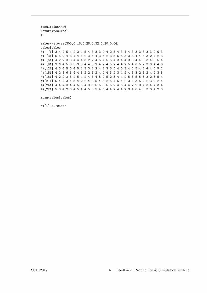
results$n6<-x6
return(results)
}
sales<-stoves(300,0.16,0.28,0.32,0.20,0.04)
sales$sales
## [1] 3 4 4 5 4 2 3 4 5 4 3 3 3 4 4 2 5 4 3 4 4 3 3 3 3 3 3 2 6 3
## [31] 5 5 2 4 3 4 4 4 2 3 5 4 3 6 2 3 5 5 5 3 3 3 4 4 3 3 2 4 2 3
## [61] 4 2 2 3 3 4 4 4 3 2 2 4 5 4 5 5 4 3 4 4 3 5 4 4 3 3 4 3 5 4
## [91] 3 6 4 5 3 5 3 3 4 4 3 2 4 2 4 5 2 4 4 2 5 4 6 5 2 3 3 4 4 3
##[121] 4 3 4 5 5 4 5 4 3 3 3 2 4 2 3 6 5 4 5 3 4 6 5 4 2 4 4 5 5 2
##[151] 4 2 5 6 3 4 4 3 2 2 5 2 4 2 4 3 2 3 4 2 4 5 3 2 5 2 4 2 3 5
##[181] 4 2 2 3 5 2 5 4 2 4 5 4 5 4 5 2 3 4 4 2 5 3 5 5 3 3 2 3 5 4
##[211] 5 4 4 3 4 5 4 2 2 4 3 5 4 3 2 5 4 5 4 2 3 4 3 5 2 2 3 2 2 4
##[241] 4 4 4 3 4 4 5 5 4 3 5 5 5 3 5 5 2 4 6 4 4 2 2 3 4 3 4 4 3 4
##[271] 5 3 4 2 3 4 5 4 4 5 3 5 4 5 4 4 2 4 4 2 3 4 6 4 3 3 3 4 2 3
mean(sales$sales)
##[1] 3.706667
SCIE2017 5 Feedback: Probability & Simulation with R