Taxation, financial intermodality and theleast taxed path for circulating incomewithin a multinational enterprise.∗

forthcoming : Annales d’Economie et de Statistiques, 75/76, Dec. 2004

Marcel Gérard†and Marie-France Gillard‡

FUCaM, Catholic University of Mons, Mons, Belgium

May 11, 2004

Abstract

When minimizing their overall tax liabilities, multinational enter-prises exploit the various provisions of interjurisdictional tax arrange-ments, not hesitating to circulate flows indirectly and through variousfinancial vehicles. This paper proposes to nest modelling such strate-gies into graph theory and network analysis. Such an exercise enablesto compute strategy supported effective tax rates and to question thedesign of interjurisdictional tax arrangements.Keywords : Taxation, Multinational firms, Application of graph

and network theory.JEL : H32, H73, C61

∗A first draft of that paper was presented at the Sevilla 2000 Congress of the Interna-tional Institute of Public Finance. The present version is a revision of the text we presentedat Pet 02, Paris, July 2002. This research is financed by the Belgian Fonds National dela Recherche Scientifique under grant 2.4561.99. Methodological suggestions by Pierre Se-mal are gratefully acknowledged as well as comments and suggestions from an anonymousreferee. Mailing address : Fucam, chaussée de Binche 151, B-7000 Mons, Belgium, tel.+32.65.323326, fax +32.65.323223, e-mail : gerard(viz. gillard)@fucam.ac.be.

†Professor of economics and taxation, also affiliated with Ucl, Louvain-la-Neuve, andCESifo, Munich.

‡FNRS Research worker.

1

Multinational firms frequently use complex paths when they circulatefunds among affiliates located in different countries or jurisdictions and, veryoften, the choice of a path is primarily dictated by tax considerations.

So far, however, economic investigation has mainly focused on direct bi-lateral flows between one affiliate, the source of the income, say a subsidiaryor a branch, and the parent company, possibly a resident taxpayer of anotherjurisdiction, computing for that purposes, effective (bilateral) tax rates.

The most popular such concept and statistics is that of marginal effectivetax rate set forth by King and Fullerton (1984) ; it is an equilibrium conceptin the classical sense, measuring, by a single statistics, the relative wedge atequilibrium, generated by the tax system under different assumptions regard-ing the source of funds, the type of assets or the status of the stockholder.Applications of King-Fullerton methodology are numerous, including Ocde(1991), Ruding (1992) and EUCommission (2001). Criticisms and extensionshave been proposed a.o. by Alworth (1988, extension to MNE’s), Boadwayand Bruce (1992), and Gérard (1993). The last paper, especially, showsthat King-Fullerton marginal effective tax rate is just a specific case of alarger class of effective tax rates, that corresponding to a classical equilib-rium. Another such specific case is the average effective tax rate put forwardby Devereux and co-authors Chennels and Griffith, see a.o. Chennels andGriffith (1997) and Devereux and Griffith (1998, 2003).

In those contributions however, as mentioned before, as far as interna-tional taxation is concerned, the flow of income is deemed to circulate directlybetween the source country and the country of residence of the investor, thusinvolving only two jurisdictions, at most. This way of computing effectivetax rates can be regarded as little compatible with actual tax behaviour ofMNE’s, since it doesn’t pay enough attention to their tax strategies.

Unlike that, in this paper, we focus on complex paths and allow a flow offunds circulating between two jurisdictions to make strategic detours throughone or more other entities and jurisdictions. We consider especially twointerrelated tax strategies - treaty shopping and vehicle changing - and use analgorithm based on graph and network theory, to compute strategy supportedeffective tax rates.

Multinational firms use the former strategy - treaty shopping - when theytry to use the provisions of international tax treaties to find out profitabledetours. They use the latter - vehicle changing - when, at some point in theflow journey, thus when the flow goes through a given member entity of the

2

multinational firm, they change one type of financial flow into another one,like turning an interest into a dividend in a low tax jurisdiction to take profitof that feature. Such strategies are part of the daily business of tax managersof multinational enterprises, in short MNE’s. However they strategies donot exhaust the opportunities provided by the tax systems; as a matterof fact, multinational enterprises also use instruments like transfer prices,management fees and royalties to exploit the provisions and opportunities ofthe various domestic tax laws and interjurisdictional tax arrangements [seee.g. Bernard and Weiner (1990), Grubert (2002)].

To cope with that, this paper suggests an approach based on graph andnetwork theory, especially on a modified version of a well known Dijkstra(1959) algorithm [for an introduction to graph and network theory, see e.g.Hillier and Liebermann (2001)] and reader accustomed with intermodal trans-portation will probably see something familiar in our approach. Therefore,in the sequel of this paper we use the words vehicle and mode equivalently,and we see vehicle changing as a form of intermodality. We consider the MNEsearch for the least taxed path over types of funds and detours through indirectpaths, as a particular application of shortest path computation. However,as far as taxation is concerned, the problem may become somewhat morecomplicated. Indeed, standard shortest path algorithms require that thecost of going through an arc of the path - say to go from one jurisdiction tothe next one - is fixed. In taxation however, double tax relief mechanismsand anti-abuse provisions violate that requirement and imply that the costof going through an arc can be contingent to the history of the path or topart of that history.

Our motivation in conducting that research is first to get a better under-standing of tax planning strategies conducted by MNE’s, second to propose arepresentation of those strategies capturing them in an extension of the nowwell known concept of effective tax rate, and third to pave the way for a bet-ter regulation of international flows of funds, especially through an improveddesign of tax treaties.

Thereafter, in section 2, we consider a two-jurisdiction world, thus limit-ing the investigation to direct flows, and we use that simple framework to setforth our formalisation. Then section 3 extends the investigation to morethan two jurisdictions allowing for strategic detours. A critical discussion ofthe approach is proposed in section 3 as well as some conclusions and avenuesfor further investigation and application.

3

1 A 2-jurisdiction world

The income produced by an economic activity can be taxed in the jurisdictionwhere it is actually produced, or in the jurisdiction where the entity whichreceives that income has its residence. In the former case, the income issaid taxed at source or according to the Source Principle, in the latter itis said taxed according to the Residence Principle [for a discussion see e.g.Mintz and Tulkens (1990) and Gérard (2002) ]. It is up to the authority ofa jurisdiction to decide for one principle or the other. However an incomecan then be taxed twice, according to the source principle in the jurisdictionwhere it is generated, and according to the residence principle when paid toa resident of another jurisdiction; then we speak of double taxation.

Also, although an income can circulate under various forms - dividend,interest, capital gain, profit - we first suppose here a single such mode orvehicle, say dividend. Then we relax that assumption.

Consider then a parent company located in jurisdiction R with an activesubsidiary located in jurisdiction S and assume that income circulates as adividend. The corporate tax rates are τR and τS respectively. Moreover,when an income flows across the border between the two jurisdictions athird tax is often due, called a withholding tax and noted mSR; its valueis determined either by jurisdiction S unilaterally or by a tax treaty betweenthe two jurisdictions. Therefore we could speak of multiple taxation ratherof double taxation.

As a consequence one unit of income generated in S becomes a net incomeySR available for distribution in jurisdiction R, with

ySR =¡1− τR

¢ ¡1−mSR

¢ ¡1− τS

¢(1)

an equation which illustrates what Feldstein and Hartman (1979) name fulltaxation after deduction.

Let us assume tentatively that such system is in operation.

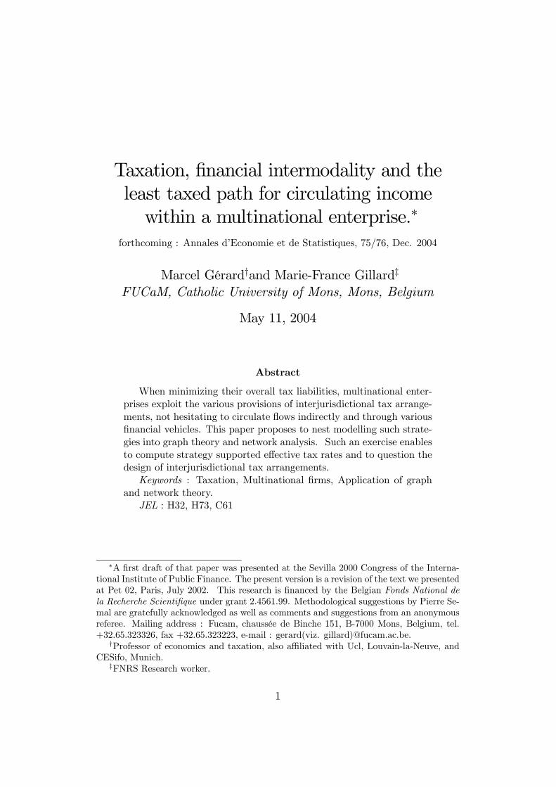
Using a graph representation, we say that the flow from initial nodeS to final node R consists of three arcs. We term the first one the SS-intrajurisdictional arc; the tax cost factor associated to using that first arcis 1− tSS where tSS = τS. The second arc is the SR-interjurisdictional arcand the associated tax cost factor is 1 − tSR with tSR = mSR. Finally the

4

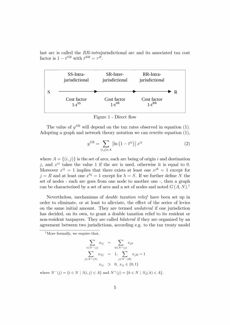
last arc is called the RR-intrajurisdictional arc and its associated tax costfactor is 1− tSR with tRR = τR.

R S

SS-Intra- jurisdictional

SR-Inter- jurisdictional

RR-Intra- jurisdictional

Cost factor 1-tSS

Cost factor 1-tSR

Cost factor 1-tRR

Figure 1 - Direct flow

The value of ySR will depend on the tax rates observed in equation (1).Adopting a graph and network theory notation we can rewrite equation (1),

ySR =X(i,j)∈A

¯̄ln¡1− tij

¢¯̄xij (2)

where A = {(i, j)} is the set of arcs, each arc being of origin i and destinationj, and xij takes the value 1 if the arc is used, otherwise it is equal to 0.Moreover xij = 1 implies that there exists at least one xjk = 1 except forj = R and at least one xhj = 1 except for h = S. If we further define N theset of nodes - each arc goes from one node to another one -, then a graphcan be characterised by a set of arcs and a set of nodes and noted G (A,N).1

Nevertheless, mechanisms of double taxation relief have been set up inorder to eliminate, or at least to alleviate, the effect of the series of levieson the same initial amount. They are termed unilateral if one jurisdictionhas decided, on its own, to grant a double taxation relief to its resident ornon-resident taxpayers. They are called bilateral if they are organized by anagreement between two jurisdictions, according e.g. to the tax treaty model

1More formally, we require that,Xi∈N−(j)

xij =X

k∈N+(j)

xjkXj∈N+(S)

xSj = 1,X

j∈N−(R)xjR = 1

xij 1 0, xij ∈ {0, 1}

where N−(j) = {i ∈ N | ∃(i, j) ∈ A} and N+(j) = {k ∈ N | ∃(j, k) ∈ A}.

5

set up by OECD2 or that suggested by UN. Finally they are multilateralif based on a multilateral arrangement among a set of countries, like theEuropean Union Parent-Subsidiary Directive [see European Tax Handbook,1999 or European Union “EC Parent-Subsidiary Directive of 23 July 1990”(90/435/EEC)].

The most popular systems of double taxation relief are the creditingmethod and the exemption method.

The crediting method allows the taxpayer in the residence jurisdiction toimpute on its domestic tax liabilities, subject to the restrictions examinedbelow, the tax paid abroad. The crediting method is termed without deferralor direct if the imputable tax is limited to the withholding tax, i.e. the taxlevied when the flow crosses the border, mSR above ; it is called with deferralor indirect if it is extended to the upstream corporate tax paid abroad, τS.Credit is said partial if only a fraction ω of the upstream tax is imputable,and full if w = 1, it is said solely imputable if it is upper limited to thedomestic tax liabilities of the MNE, and repayable if it may generate a netrefund from domestic tax authorities. Notice that in international taxationit is usually solely imputable.3

The exemption method consists in deciding that an income is tax exempt,sometimes but up to a fraction µ, in one of the jurisdictions, most usuallythat of the residence of the taxpayer.

Finally, there are also anti-abuse provisions that currently tax the passiveincome or/and the income routed through low-tax jurisdictions; thereforeparameter µ and w can depend on the value of the corporate tax rate injurisdiction S.

2Articles 23A and 23B of the OECD model tax treaty provide that, when the foreign-source income is taxed in the source jurisdiction, the destination jurisdiction has either touse the exemption method (article 23A) or the crediting method (article 23B) in order toprevent double taxation

3As to the choice between a crediting method and an exemption method, internationaleconomic arguments rely on the merits of tax neutrality [Inland Revenue (1999)]. Econo-mists speak of Capital Export Neutrality if the tax system provides no incentive for residenttaxpayers in a given jurisdiction to invest at home rather than abroad or vice versa, andof Capital Import Neutrality when all agents investing in a given jurisdiction are subjectto the same taxation by that jurisdiction on similar investments, whether they are or notresidents of the jurisdiction. Gérard (2002) proposes a detailed analysis of the respectiveproperties of the mechanisms.

6

1.1 The foreign tax crediting method

Tax cost factors 1 − tSS = 1 − τS and 1 − tSR = 1 − mSR are unaffectedby the choice between foreign tax crediting and exemption. Unlike thoseparameters, 1− tRR does depend on that choice.

Under the crediting method, assuming that the credit is solely imputable,

tRR = max{0, τR¡1 + ωSR

¢− ωSR} (3)

with

ωSR =wRmm

SR

(1−mSR)+

wRτ τ

S

(1−mSR) (1− τS)(4)

where wRm and w

Rτ are the imputation rates with a subscriptm or τ indicating

which tax is imputed and a superscript R referring to the jurisdiction wherethat tax can be imputed.

Notice that if both imputation rates are equal to unity,

tRR = max{0,τR −

£τS +mSR

¡1− τS

¢¤(1−mSR) (1− τS)

} (5)

so that the the residence principle applies if the second element of the bracketis positive - then ySR = 1 − τR and the tax system is said capital exportneutral - while the source principle applies if that element is non positive- then ySR =

¡1−mSR

¢ ¡1− τS

¢and the system is capital import neutral.

This point seems to corroborate Mintz and Tulkens (1996) who refer to anddiscuss Feldstein and Hartman (1979) and Musgrave and Musgrave (1984)on that issue.4

1.2 The exemption method

Under the exemption method, income is not subject to the corporate taxeither in the S or the R jurisdiction, except possibly for a small part µ of

4Let us add that excess credit can often be deducted against the tax base.Formally if only a fraction γ of the tax credit can be effectively used so thatγ©wRm(1− τR)mSR

¡1− τS

¢+ wR

τ (1− τR)τSª= τR(1 − τS)(1 − mSR)then, the parent

company can deduct the excess credit against its corporate tax base, getting a tax rebatewhich amounts to τR (1− γ)

©wRm(1− τR)mSR

¡1− τS

¢+ wR

τ (1− τR)τSªOf course that

rebate is smaller than the advantage provided by repayability of the excess credit sinceτR < 1.

7

it (5 percent according to EU Parent-Subsidiary Directive of July 23, 1990).Usually, the exempting jurisdiction is R and we should speak more preciselyof inflow exemption. Should the exempting jurisdiction be S, we would speakof outflow exemption. Assume the former, so that µ = µR and allow thatparameter to be contingent to the origin of the flow, so that it is noted µSR.Then,

tRR = µSRτR (6)

If µSR vanishes, like in France, so does tRR too, and the exemption methodis an application of the source principle, producing a capital import neutralinternational tax system as long asmSR does not depend on S, and generatingno tax externality against destination jurisdiction R.

1.3 Synthesis and extension to more than a single fi-nancial mode

The net income in jurisdiction R generated by a pretax income equal to unityin jurisdiction S can be written,

ySR = 1− T (7)

where T stands for the effective (bilateral) tax rate with,

T = τS +mSR(1− τS) + tRR¡1−mSR

¢(1− τS) (8)

where

tRR = θmax©0, τR

¡1 + ωSR

¢− ωSR

ª+(1− θ)µRτR (9)

with θ = 1 under the crediting method and θ = 0 otherwise.

If various financial modes are permitted, ySR also depends on the vehicle fchosen by the MNE for circulating the income. Then the tax cost factors haveto be adapted accordingly, e.g. to reflect that interest uses to be deductibleagainst the tax base in the paying jurisdiction. Seeking for the least taxedpath then consists in selecting f such that it

minf

X(i,j)∈A

¯̄ln¡1− tijf

¢¯̄xijf (10)

8

The value of f is selected by the MNE at any intrajurisdictional arc butthe ultimate one, where that choice is then irrelevant; thus here only in S.Now each variable has also to be characterised by a subscript f indicatingthe vehicle used, dividend (f = 1), interest (f = 2), capital gain (f = 3) orprofit (f = 4).

2 Least taxed path in a n>2 - jurisdictionworld

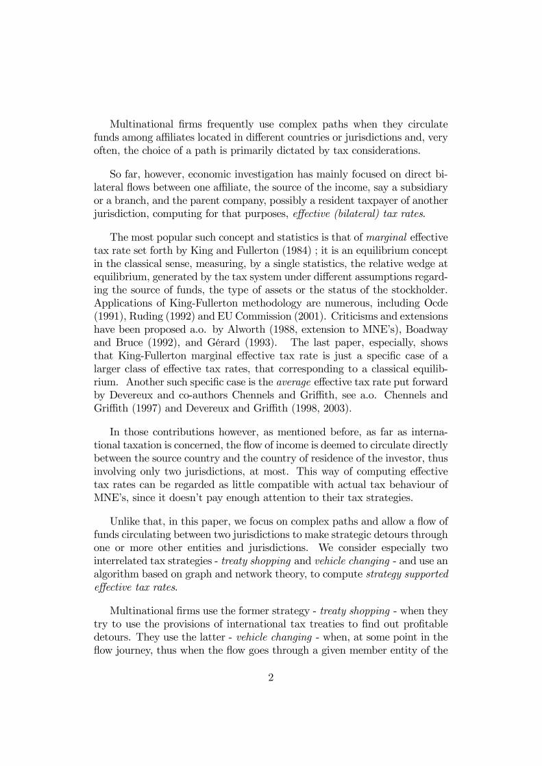
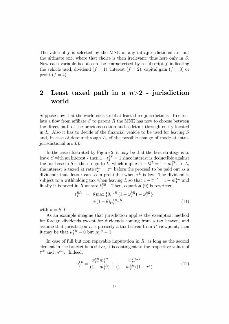
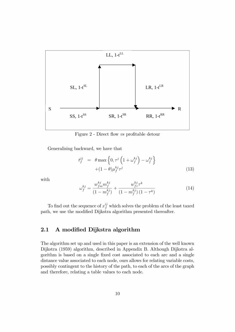
Suppose now that the world consists of at least three jurisdictions. To circu-late a flow from affiliate S to parent R the MNE has now to choose betweenthe direct path of the previous section and a detour through entity locatedin L. Also it has to decide of the financial vehicle to be used for leaving Sand, in case of detour through L, of the possible change of mode at intra-jurisdictional arc LL.

In the case illustrated by Figure 2, it may be that the best strategy is toleave S with an interest - then 1− tSS2 = 1 since interest is deductible againstthe tax base in S -, then to go to L, which implies 1− tSL2 = 1−mSL

2 . In L,the interest is taxed at rate tLL2 = τL before the proceed to be paid out as adividend; that detour can seem profitable when τL is low. The dividend issubject to a withholding tax when leaving L so that 1− tLR1 = 1−mLR

1 andfinally it is taxed in R at rate tRR1 . Then, equation (9) is rewritten,

tRRf = θmax©0, τR

¡1 + ωkR

f

¢− ωkR

f

ª+(1− θ)µkRf τR (11)

with k = S, L.As an example imagine that jurisdiction applies the exemption method

for foreign dividends except for dividends coming from a tax heaven, andassume that jurisdiction L is precisely a tax heaven from R viewpoint; thenit may be that µSR1 = 0 but µLR1 = 1.

In case of full but non repayable imputation in R, as long as the secondelement in the bracket is positive, it is contingent to the respective values oftkk and mkR. Indeed,

ωkRf =

wkRfmm

kRf

(1−mkRf )

+wkRfτ τ

k

(1−mkRf ) (1− τk)

(12)

9

R S SS, 1-tSS SR, 1-tSR

RR, 1-tRR

SL, 1-tSL

LL, 1-tLL

LR, 1-tLR

Figure 2 - Direct flow vs profitable detour

Generalising backward, we have that

tjjf = θmaxn0, τ j

³1 + ωkj

f

´− ωkj

f

o+(1− θ)µkjf τ

j (13)

with

ωkjf =

wkjfmm

kjf

(1−mkjf )+

wkjfττ

k

(1−mkjf ) (1− τk)

(14)

To find out the sequence of xijf which solves the problem of the least taxedpath, we use the modified Dijkstra algorithm presented thereafter.

2.1 A modified Dijkstra algorithm

The algorithm set up and used in this paper is an extension of the well knownDijkstra (1959) algorithm, described in Appendix B. Although Dijkstra al-gorithm is based on a single fixed cost associated to each arc and a singledistance value associated to each node, ours allows for relating variable costs,possibly contingent to the history of the path, to each of the arcs of the graphand therefore, relating a table values to each node.

10

Our extension5 of Dijkstra’s algorithm is formally presented in AppendixA; we believe that the reader will gain a better insight of our approachfollowing the application thereafter.

2.2 Application

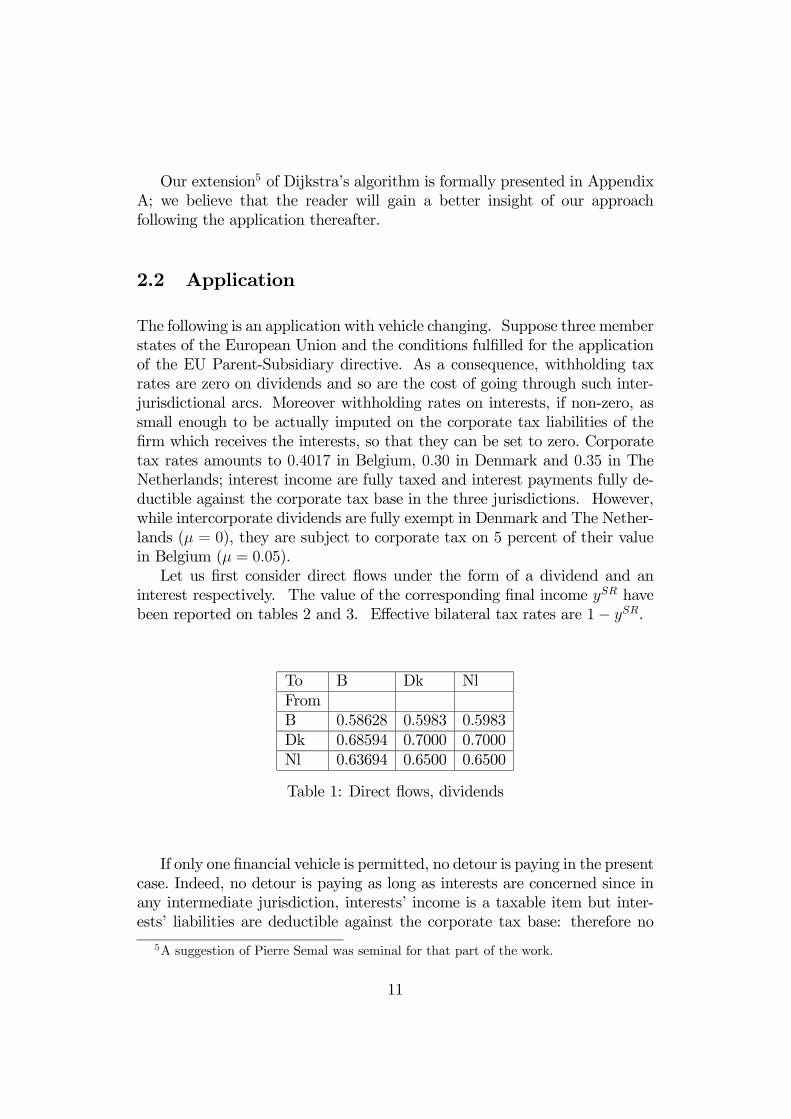
The following is an application with vehicle changing. Suppose three memberstates of the European Union and the conditions fulfilled for the applicationof the EU Parent-Subsidiary directive. As a consequence, withholding taxrates are zero on dividends and so are the cost of going through such inter-jurisdictional arcs. Moreover withholding rates on interests, if non-zero, assmall enough to be actually imputed on the corporate tax liabilities of thefirm which receives the interests, so that they can be set to zero. Corporatetax rates amounts to 0.4017 in Belgium, 0.30 in Denmark and 0.35 in TheNetherlands; interest income are fully taxed and interest payments fully de-ductible against the corporate tax base in the three jurisdictions. However,while intercorporate dividends are fully exempt in Denmark and The Nether-lands (µ = 0), they are subject to corporate tax on 5 percent of their valuein Belgium (µ = 0.05).Let us first consider direct flows under the form of a dividend and an

interest respectively. The value of the corresponding final income ySR havebeen reported on tables 2 and 3. Effective bilateral tax rates are 1− ySR.

To B Dk NlFromB 0.58628 0.5983 0.5983Dk 0.68594 0.7000 0.7000Nl 0.63694 0.6500 0.6500

Table 1: Direct flows, dividends

If only one financial vehicle is permitted, no detour is paying in the presentcase. Indeed, no detour is paying as long as interests are concerned since inany intermediate jurisdiction, interests’ income is a taxable item but inter-ests’ liabilities are deductible against the corporate tax base: therefore no

5A suggestion of Pierre Semal was seminal for that part of the work.

11

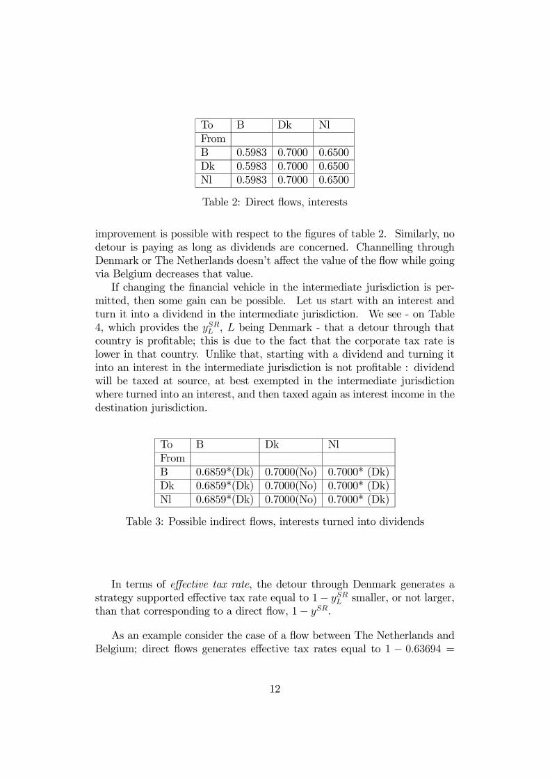
To B Dk NlFromB 0.5983 0.7000 0.6500Dk 0.5983 0.7000 0.6500Nl 0.5983 0.7000 0.6500

Table 2: Direct flows, interests

improvement is possible with respect to the figures of table 2. Similarly, nodetour is paying as long as dividends are concerned. Channelling throughDenmark or The Netherlands doesn’t affect the value of the flow while goingvia Belgium decreases that value.If changing the financial vehicle in the intermediate jurisdiction is per-

mitted, then some gain can be possible. Let us start with an interest andturn it into a dividend in the intermediate jurisdiction. We see - on Table4, which provides the ySRL , L being Denmark - that a detour through thatcountry is profitable; this is due to the fact that the corporate tax rate islower in that country. Unlike that, starting with a dividend and turning itinto an interest in the intermediate jurisdiction is not profitable : dividendwill be taxed at source, at best exempted in the intermediate jurisdictionwhere turned into an interest, and then taxed again as interest income in thedestination jurisdiction.

To B Dk NlFromB 0.6859*(Dk) 0.7000(No) 0.7000* (Dk)Dk 0.6859*(Dk) 0.7000(No) 0.7000* (Dk)Nl 0.6859*(Dk) 0.7000(No) 0.7000* (Dk)

Table 3: Possible indirect flows, interests turned into dividends

In terms of effective tax rate, the detour through Denmark generates astrategy supported effective tax rate equal to 1− ySRL smaller, or not larger,than that corresponding to a direct flow, 1− ySR.

As an example consider the case of a flow between The Netherlands andBelgium; direct flows generates effective tax rates equal to 1 − 0.63694 =

12

0.363 06 and 1− 0.5983 = 0.401 7 for a dividend and an interest respectively,while the strategy supported rate amounts to 1− 0.6859 = 0.314 1.

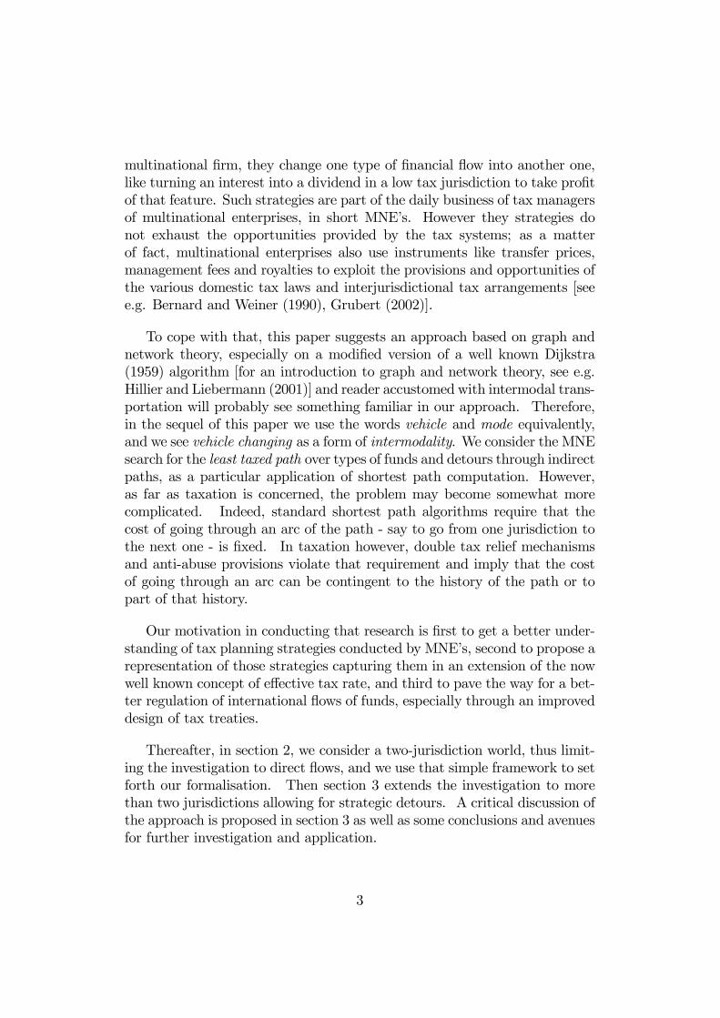
Now let us see how that result can be obtained using our algorithm. Forthe ease of the exposition we first suppose a flow to Belgium leaving TheNetherlands as an interest. The cost factor associated to an arc is

cijf =¯̄ln¡1− tijf

¢¯̄(15)

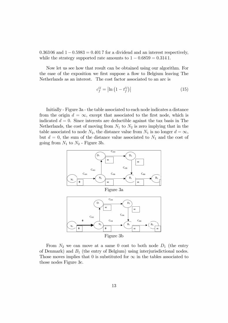
Initially - Figure 3a - the table associated to each node indicates a distancefrom the origin d = ∞, except that associated to the first node, which isindicated d = 0. Since interests are deductible against the tax basis in TheNetherlands, the cost of moving from N1 to N2 is zero implying that in thetable associated to node N2, the distance value from N1 is no longer d =∞,but d = 0, the sum of the distance value associated to N1 and the cost ofgoing from N1 to N2 - Figure 3b.

N2

D1 D2

B1 CNN

CND

CDD

CDB

CNB CBB

N1 B2

0

∞

∞

∞

∞

Figure 3a

N2

D1 D2

B1 0

CND

CDD

CDB

CNB CBB

N1 B2

0

∞

0

∞

∞ ∞

Figure 3b

From N2 we can move at a same 0 cost to both node D1 (the entryof Denmark) and B1 (the entry of Belgium) using interjurisdictional nodes.Those moves implies that 0 is substituted for ∞ in the tables associated tothose nodes Figure 3c.

13

0

N2

D1 D2

B1 0

CDD

CDB

CNB CBB

N1B2

0

0

0

∞

0 ∞

Figure 3c

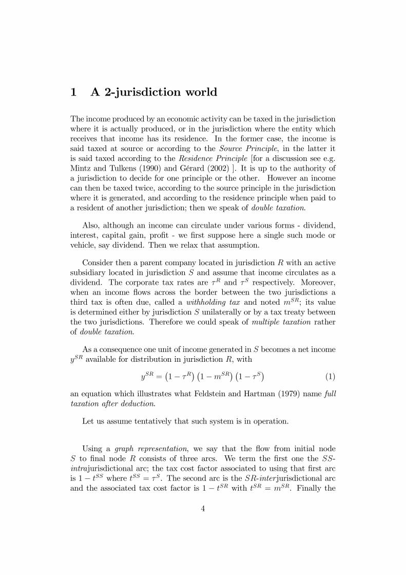
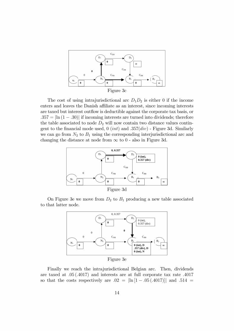
The cost of using intrajurisdictional arc D1D2 is either 0 if the incomeenters and leaves the Danish affiliate as an interest, since incoming interestsare taxed but interest outflow is deductible against the corporate tax basis, or.357 = |ln (1− .30)| if incoming interests are turned into dividends; thereforethe table associated to node D2 will now contain two distance values contin-gent to the financial mode used, 0 (int) and .357(div) - Figure 3d. Similarlywe can go from N2 to B1 using the corresponding interjurisdictional arc andchanging the distance at node from ∞ to 0 - also in Figure 3d.

N2

D1 D2

B1 0

0, 0.357

CDB

CNB CBB

N1B2

0

0

0

0 (int), 0.357 (div)

0 ∞

Figure 3d

On Figure 3e we move from D2 to B1 producing a new table associatedto that latter node.

0, 0.357

0 0

N2

D1 D2

B1 0 CNB CBB

N1 B2

0

0

0

0 (int), 0.357 (div)

0 (int), D .357 (div), D0 (int), N

∞

Figure 3e

Finally we reach the intrajurisdictional Belgian arc. Then, dividendsare taxed at .05 (.4017) and interests are at full corporate tax rate .4017so that the costs respectively are .02 = |ln [1− .05 (.4017)]| and .514 =

14

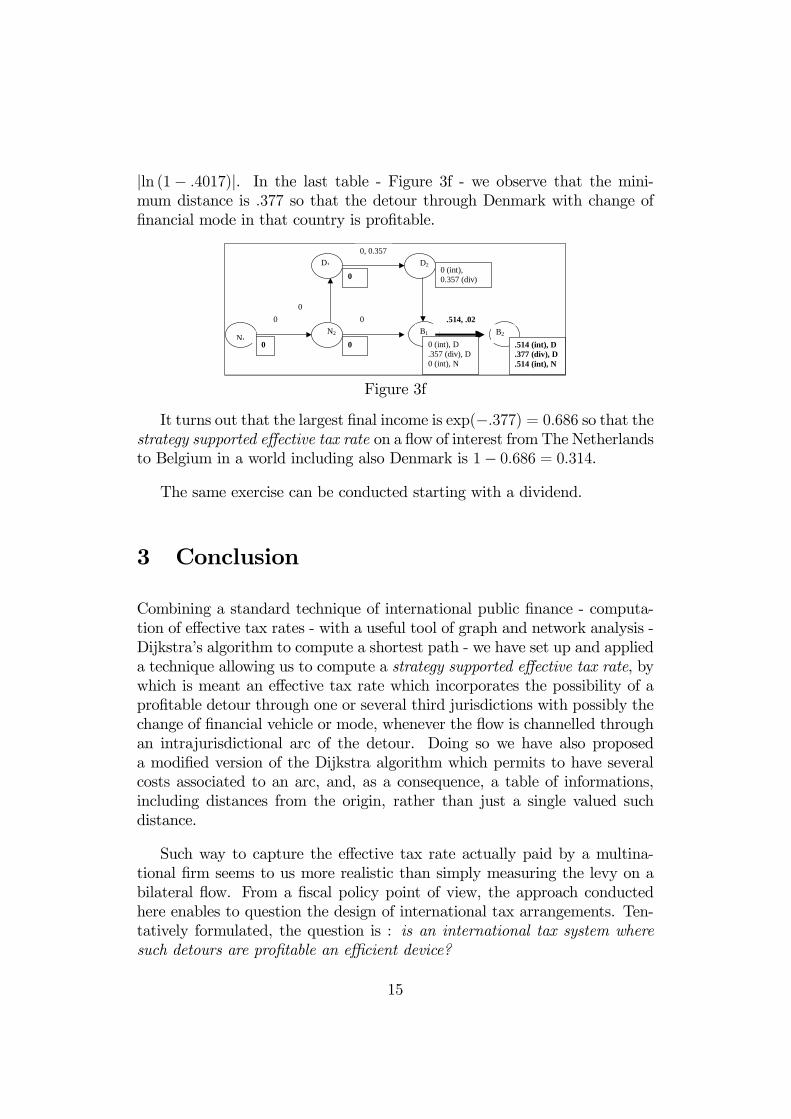
|ln (1− .4017)|. In the last table - Figure 3f - we observe that the mini-mum distance is .377 so that the detour through Denmark with change offinancial mode in that country is profitable.

0, 0.357

0

N2

D1 D2

B1 0 0 .514, .02

N1B2

0

0

0

0 (int), 0.357 (div)

0 (int), D .357 (div), D0 (int), N

.514 (int), D

.377 (div), D

.514 (int), N

Figure 3f

It turns out that the largest final income is exp(−.377) = 0.686 so that thestrategy supported effective tax rate on a flow of interest fromThe Netherlandsto Belgium in a world including also Denmark is 1− 0.686 = 0.314.

The same exercise can be conducted starting with a dividend.

3 Conclusion

Combining a standard technique of international public finance - computa-tion of effective tax rates - with a useful tool of graph and network analysis -Dijkstra’s algorithm to compute a shortest path - we have set up and applieda technique allowing us to compute a strategy supported effective tax rate, bywhich is meant an effective tax rate which incorporates the possibility of aprofitable detour through one or several third jurisdictions with possibly thechange of financial vehicle or mode, whenever the flow is channelled throughan intrajurisdictional arc of the detour. Doing so we have also proposeda modified version of the Dijkstra algorithm which permits to have severalcosts associated to an arc, and, as a consequence, a table of informations,including distances from the origin, rather than just a single valued suchdistance.

Such way to capture the effective tax rate actually paid by a multina-tional firm seems to us more realistic than simply measuring the levy on abilateral flow. From a fiscal policy point of view, the approach conductedhere enables to question the design of international tax arrangements. Ten-tatively formulated, the question is : is an international tax system wheresuch detours are profitable an efficient device?

15

That approach has however some limitations. One is limitation to suchmodes of circulating flows as dividends, interests, capital gains or profits,ignoring other tax shifting methods like the use of transfer pricing and intan-gibles. Another one6, only relevant when a tax system like that in the US isin operation, is related to the fact that our tool seems to imply that excesscredit are computed per country; however we think that such limitation canbe eliminated.

References

[1] Alworth, J., 1988, The finance, investment and taxation decisions ofmultinationals, Blackwell, London.

[2] Bernard, J.-T. and R.J. Weiner, 1990, Multinational Corporations,Transfer Prices and Taxes: Evidence form the US Petroleum Indus-try, in A. Razin and J. Slemrod, ed., Taxation in the Global Economy,The University of Chicago Press, Chicago and London.

[3] Boadway, R. and N. Bruce, 1992, ”Problems with integrating corpo-rate and personal income taxes in an open economy”, Journal of PublicEconomics, 48, pp. 39-66.

[4] Chennels, L. et R. Griffith, 1997, Taxing Profits in a Changing World,The Institute of Fiscal Studies, Londres, 178p.

[5] Coopers and Lybrand, 1997, International Tax Summaries.

[6] Devereux M. and R. Griffith, 1998, ”The Taxation of Discrete Invest-ment Choices The Institute for Fiscal Studies”, IFS Working Paper se-ries, W98/16, London.

[7] Devereux M. and R. Griffith, 2003, ”Evaluating Tax Policy for LocationDecisions”, International Tax and Public Finance, 10, pp. 107-126.

[8] Dijkstra, E. W., 1959 ”A Note on Two Problems in Connection withGraphs” Numerische Math. 1, pp. 269-271.

[9] European Union, 1990, ”EC Parent-Subsidiary Directive of 23 July1990” (90/435/EEC).

6That second limitation, only valid when a tax system like that in operation in US, hasbeen pointed out to us my Alan Auerbach.

16

[10] European Commission, 2001, Towards an Internal Market without TaxObstacles, a strategy for providing companies with a consolidated corpo-rate tax base for their EU-wide activities, COM(2001)582, Brussels.

[11] Feldstein, M. and Hartman, D., 1979, ”The optimal taxation of foreignsource investment income”, Quarterly Journal of Economics, 93, pp.613-624.

[12] Gérard, M., 1982, Le financement des investissements, leur volume etl’impôt, Presses Universitaires de Namur, Namur.

[13] Gérard, M., 1993, ”Cost of capital, investment location and marginaleffective tax rate: methodology and application”, chap. 4 in A. Heimlerand D. Meulders (eds), Empirical Approaches to Fiscal Policy Modelling,Chapman et Hall, London, pp. 61-80.

[14] Gérard, M., 2002, “Neutralities and Non-Neutralities in InternationalCorporate Taxation, An Evaluation of Possible and Recent Moves”, Ifo-Studiën, 48 (4), pp. 533-554.

[15] Gérard, M., 2003, “L’imposition des entreprises multinationales en Eu-rope, à propos d’un rapport de la Commission européenne”, RevueEconomique, 54 (3), pp. 489-498.

[16] Gillard, M-F., 1998, ”Recherche du chemin fiscal de moindre coût”, the-sis of civil engineer in applied maths., Université Catholique de Louvain-La-Neuve.

[17] King, M. et D. Fullerton, 1984, The Taxation of Income from Capital :a Comparative Study of United States, the United Kingdom, Sweden andWest- Germany, The University of Chicago Press, Chicago and London.

[18] Grubert, H., 1998, ”Taxes and the division of foreign operating incomeamong royalties, interest, dividends and retained earnings”, Journal ofPublic Economics, 68, pp. 269-290.

[19] Grubert, H., 2002, ”The Tax Burden on Direct Cross-Border Investment:Company Strategies and Government Responses”, Workshop on ”Mea-suring the Tax Burden on Capital and Labour”, CESifo Venice SummerInstitute, San Servolo, July 15-16, forthcoming in a book edited by P.B.Sorensen, MIT Press.

[20] Hillier, F. and G. Liebermann, 2001, Introduction to Operations Re-search, 7th ed., McGraw-Hill.

17

[21] Inland Revenue, 1999, ”Double Taxation Relief for Companies: A dis-cussion paper”, Mike Waters.

[22] International Bureau of Fiscal Documentation, 1999, European TaxHandbook, IBFD, Amsterdam (in cooperation with KPMG).

[23] International Bureau of Fiscal Documentation, 2001, European TaxHandbook, IBFD, Amsterdam (in cooperation with KPMG).

[24] King, M.A., 1974, ”Taxation and the cost of capital”, Review of Eco-nomic Studies,41, pp. 21-35.

[25] King, M.A., 1977, Public Policy and the Corporation, Chapman andHall, London.

[26] Mintz, J. and Leechor, C., 1993, ”On the taxation of multinationalcorporate investment when the deferral method is used by the capitalexporting jurisdiction”, Journal of Public Economics, 51, pp. 75-96.

[27] Mintz, J. and Tulkens, H., 1990, ”Strategic Use of Tax Rates and Creditsin a Model of International Corporate Income Tax Competition”, CoreDiscussion Paper, 9073, pp. 7-16.

[28] Mintz, J. and Tulkens, H., 1996, ”Optimality Properties of AlternativeSystems of Taxation of Foreign Capital Income”, Journal of Public Eco-nomics, 60, pp. 373-399.

[29] Musgrave, R. and Musgrave, P., 1984, Public Finance in Theory andPractice, McGraw Hill, New York.

[30] OCDE, 1991, Taxing Profits in a Global Economy, domestic and inter-national issues, OCDE, Paris.

[31] Oecd, 1996, Model tax convention on income and on capital, condednsedversion, Oecd, Paris.

[32] Ruding, O. and al., 1992, Report of the Committee of Independent Ex-perts on Company Taxation, Commission of the European Communities,known as Ruding report.

18

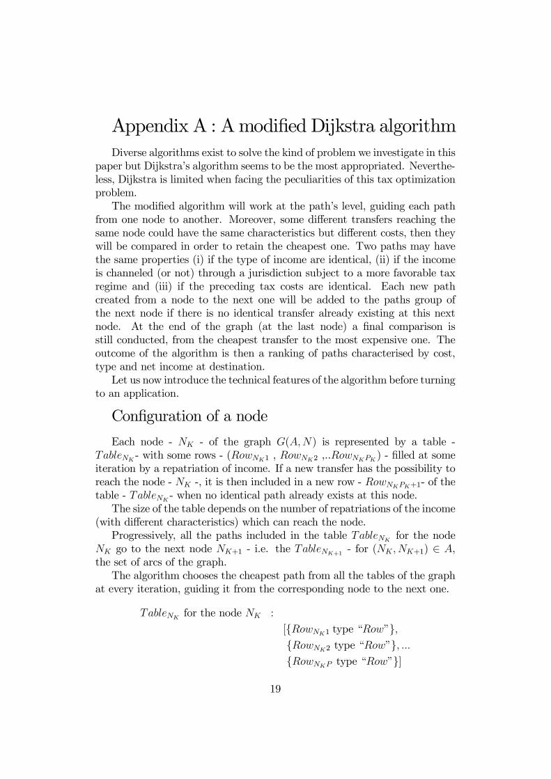
Appendix A : Amodified Dijkstra algorithmDiverse algorithms exist to solve the kind of problem we investigate in this

paper but Dijkstra’s algorithm seems to be the most appropriated. Neverthe-less, Dijkstra is limited when facing the peculiarities of this tax optimizationproblem.The modified algorithm will work at the path’s level, guiding each path

from one node to another. Moreover, some different transfers reaching thesame node could have the same characteristics but different costs, then theywill be compared in order to retain the cheapest one. Two paths may havethe same properties (i) if the type of income are identical, (ii) if the incomeis channeled (or not) through a jurisdiction subject to a more favorable taxregime and (iii) if the preceding tax costs are identical. Each new pathcreated from a node to the next one will be added to the paths group ofthe next node if there is no identical transfer already existing at this nextnode. At the end of the graph (at the last node) a final comparison isstill conducted, from the cheapest transfer to the most expensive one. Theoutcome of the algorithm is then a ranking of paths characterised by cost,type and net income at destination.Let us now introduce the technical features of the algorithm before turning

to an application.

Configuration of a node

Each node - NK - of the graph G(A,N) is represented by a table -TableNK

- with some rows - (RowNK1 , RowNK2 ,..RowNKPK ) - filled at someiteration by a repatriation of income. If a new transfer has the possibility toreach the node - NK -, it is then included in a new row - RowNKPK+1- of thetable - TableNK

- when no identical path already exists at this node.The size of the table depends on the number of repatriations of the income

(with different characteristics) which can reach the node.Progressively, all the paths included in the table TableNK

for the nodeNK go to the next node NK+1 - i.e. the TableNK+1

- for (NK, NK+1) ∈ A,the set of arcs of the graph.The algorithm chooses the cheapest path from all the tables of the graph

at every iteration, guiding it from the corresponding node to the next one.

TableNKfor the node NK :

[{RowNK1 type “Row”},{RowNK2 type “Row”}, ...{RowNKP type “Row”}]

19

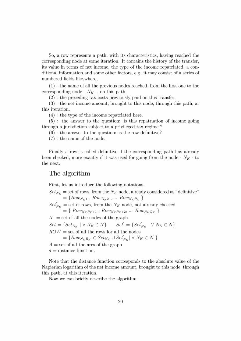
So, a row represents a path, with its characteristics, having reached thecorresponding node at some iteration. It contains the history of the transfer,its value in terms of net income, the type of the income repatriated, a con-ditional information and some other factors, e.g. it may consist of a series ofnumbered fields like,where,

(1) : the name of all the previous nodes reached, from the first one to thecorresponding node - NK -, on this path(2) : the preceding tax costs previously paid on this transfer.(3) : the net income amount, brought to this node, through this path, at

this iteration.(4) : the type of the income repatriated here.(5) : the answer to the question: is this repatriation of income going

through a jurisdiction subject to a privileged tax regime ?(6) : the answer to the question: is the row definitive?(7) : the name of the node.

Finally a row is called definitive if the corresponding path has alreadybeen checked, more exactly if it was used for going from the node - NK - tothe next.

The algorithm

First, let us introduce the following notations,

SetNK= set of rows, from theNK node, already considered as ”definitive”= {RowNK1 , RowNK2 , ... RowNKPK }

Set0NK

= set of rows, from the NK node, not already checked= { RowNKPK+1 , RowNKPK+2, ... RowNKQK

}N = set of all the nodes of the graph

Set = {SetNK| ∀ NK ∈ N} Set

0= {Set0NK

| ∀ NK ∈ N}ROW = set of all the rows for all the nodes

= {RowNKRK∈ SetNK

∪ Set0NK| ∀ NK ∈ N }

A = set of all the arcs of the graphd = distance function.

Note that the distance function corresponds to the absolute value of theNapierian logarithm of the net income amount, brought to this node, throughthis path, at this iteration.Now we can briefly describe the algorithm.

20

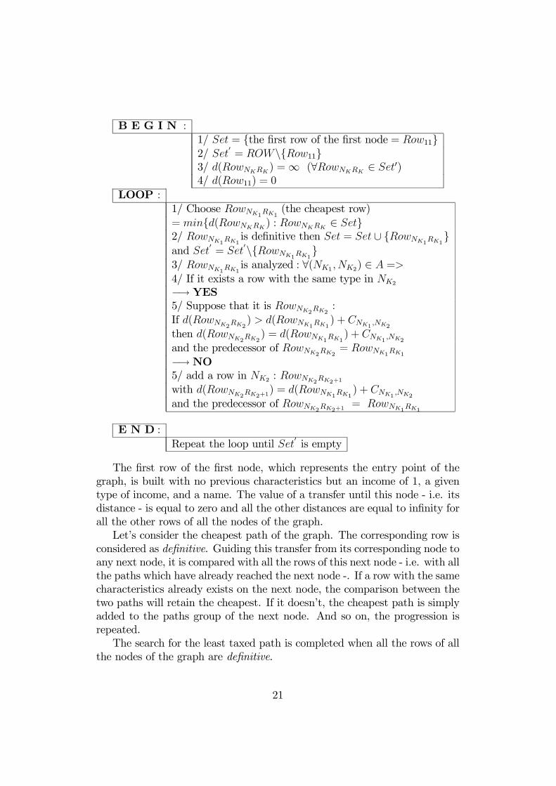
B E G I N :1/ Set = {the first row of the first node = Row11}2/ Set

0= ROW\{Row11}

3/ d(RowNKRK) =∞ (∀RowNKRK

∈ Set0)4/ d(Row11) = 0

LOOP :1/ Choose RowNK1

RK1(the cheapest row)

= min{d(RowNKRK) : RowNKRK

∈ Set}2/ RowNK1

RK1is definitive then Set = Set ∪ {RowNK1

RK1}

and Set0= Set

0\{RowNK1RK1}

3/ RowNK1RK1is analyzed : ∀(NK1 , NK2) ∈ A =>

4/ If it exists a row with the same type in NK2

−→ YES5/ Suppose that it is RowNK2

RK2:

If d(RowNK2RK2) > d(RowNK1

RK1) + CNK1

,NK2

then d(RowNK2RK2) = d(RowNK1

RK1) + CNK1

,NK2

and the predecessor of RowNK2RK2

= RowNK1RK1

−→ NO5/ add a row in NK2 : RowNK2

RK2+1

with d(RowNK2RK2+1

) = d(RowNK1RK1) + CNK1

,NK2

and the predecessor of RowNK2RK2+1

= RowNK1RK1

E N D :

Repeat the loop until Set0is empty

The first row of the first node, which represents the entry point of thegraph, is built with no previous characteristics but an income of 1, a giventype of income, and a name. The value of a transfer until this node - i.e. itsdistance - is equal to zero and all the other distances are equal to infinity forall the other rows of all the nodes of the graph.Let’s consider the cheapest path of the graph. The corresponding row is

considered as definitive. Guiding this transfer from its corresponding node toany next node, it is compared with all the rows of this next node - i.e. with allthe paths which have already reached the next node -. If a row with the samecharacteristics already exists on the next node, the comparison between thetwo paths will retain the cheapest. If it doesn’t, the cheapest path is simplyadded to the paths group of the next node. And so on, the progression isrepeated.The search for the least taxed path is completed when all the rows of all

the nodes of the graph are definitive.

21

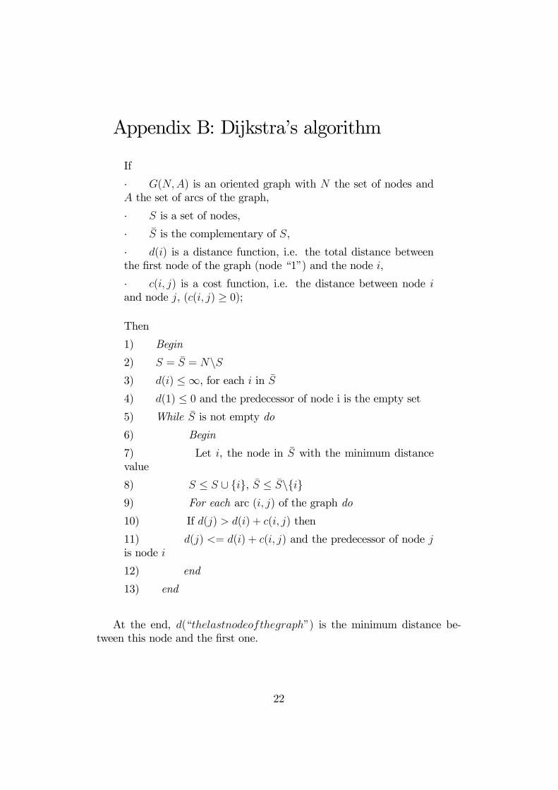
Appendix B: Dijkstra’s algorithm

If

· G(N,A) is an oriented graph with N the set of nodes andA the set of arcs of the graph,

· S is a set of nodes,

· S̄ is the complementary of S,

· d(i) is a distance function, i.e. the total distance betweenthe first node of the graph (node “1”) and the node i,

· c(i, j) is a cost function, i.e. the distance between node iand node j, (c(i, j) ≥ 0);

Then

1) Begin

2) S = S̄ = N\S3) d(i) ≤ ∞, for each i in S̄

4) d(1) ≤ 0 and the predecessor of node i is the empty set5) While S̄ is not empty do

6) Begin

7) Let i, the node in S̄ with the minimum distancevalue

8) S ≤ S ∪ {i}, S̄ ≤ S̄\{i}9) For each arc (i, j) of the graph do

10) If d(j) > d(i) + c(i, j) then

11) d(j) <= d(i) + c(i, j) and the predecessor of node jis node i

12) end

13) end

At the end, d(“thelastnodeofthegraph”) is the minimum distance be-tween this node and the first one.

22