11-233

“Tax incidence with strategic firms on the soft drink market”

Céline Bonnet and Vincent Réquillart  

April 2011, revised version July 2012

Tax incidence with strategic firms on the soft drink market.

Céline Bonnet∗ and Vincent Requillart†

July 13, 2012

Abstract

Because soft drink (SD) consumption is considered to be a contributor to the ’epidemic’ of obesity,there is a growing interest in evaluating the impact on SD consumption of alternative tax policies. Inthis paper, we propose a methodology to evaluate the impact of taxation of a food market taking intoaccount the strategic price response of both manufacturers and retailers. We apply this methodologyto the French SD market and simulate the impacts of ad valorem and excise taxes. We find thatfirms behave differently when facing an ad valorem tax or an excise tax. Excise tax is overshifted toconsumer prices while ad valorem tax is undershifted to consumer prices. We find that an excise taxbased on the sugar content of SD is the most efficient at reducing soft drink consumption. Our resultsalso indicate that ignoring strategic pricing by firms leads to misestimate the impact of taxation by15% to 40% depending on the products and the tax implemented. In the short term, that is ignoringpositive long term health effects, a € 9 cents per litre excise tax has a small negative welfare effect(about € 1 per person per year).

JEL codes:H32, L13, IQ18, I18

Key words: excise tax, ad valorem tax, tax incidence, strategic pricing, differentiated products,soft drinks.

∗Toulouse School of Economics (INRA, GREMAQ), 21 Allée de Brienne, F-31000 Toulouse France, Tel: +33 (0)5 61 1285 91, cbonnet@toulouse.inra.fr, corresponding author.

†Toulouse School of Economics (INRA, GREMAQ; IDEI), 21 Allée de Brienne, F-31000 Toulouse France, Tel: +33 (0)561 12 86 07, vincent.requillart@toulouse.inra.fr.

1

1 Introduction

According to the World Health Organization, non communicable diseases, mainly cardiovascular diseases,

cancers, chronic respiratory diseases and diabetes cause about 35 million deaths each year representing

about 60% of all deaths.1 Moreover up to 80% of heart disease, stroke, and type 2 diabetes and over a

third of cancers could be prevented by eliminating shared risk factors, mainly tobacco use, unhealthy diet,

physical inactivity and the harmful use of alcohol. A healthier food diet could be reached by reducing

salt levels, eliminating industrially produced trans-fatty acids, decreasing saturated fats and limiting free

sugars. A related consequence of unhealthy diet and physical inactivity is the rise in obesity prevalence.

To tackle this public health problem, governments have tried to use public information campaigns with

the aim of getting people to change their food habits. These information campaigns may have positive

impacts on food consumption (Weiss and Tschirhart, 1994; Snyder, 2007). However, they seem to have

not been sufficiently effective at changing behavior (Cutler et al., 2003), and have failed to reverse the

rising trend in obesity, diabetes and so on. In other areas legislation and taxation have proved more

effective. For example, in the cigarettes or alcohol markets, legislation restricts sales to young people as

well as advertising, and taxation increases the relative price of these goods (Adda and Cornaglia, 2006).

Till now, tax (subsidy) policies designed to promote healthier food choices are almost unused. However,

as they have been shown to be effective for the cigarettes market, they might be considered as tools to

influence consumer behavior to improve diets and therefore public health.

As the link between food intake and health is more and more recognized, there is a growing interest

in the ex ante analysis of the health impacts of alternative food price policies. The general methodology

used is a two-stage procedure which combines an economic model and a health model. The economic

model is used to assess the impact on food or nutrient consumption of alternative tax or subsidy policies.

Then, the health model assesses the impact of food consumption changes on some health indicators.

Thow et al. (2010) presented a review of such approaches. More recent contributions include Purshouse

1World Health Organization, 2008-2013 Action Plan for the Global Strategy for the Prevention and Control of Non-communicable Diseases. http://whqlibdoc.who.int/publications/2009/9789241597418_eng.pdf (accessed 2010, December17)

2

et al. (2010), Dallongeville et al. (2011), Allais et al. (2010), Bonnet and Requillart (2011) and Griffith

et al. (2010).

A common limit of almost all these analysis is the assumption of passive pricing, that is producers

and retailers are supposed not to adjust product prices in response to the tax (subsidy) policy. The only

example of a paper integrating strategic pricing is Griffith et al. (2010) who account for strategic behavior

at the manufacturer level. However they ignore manufacturer and retailers relationships. Both the food

and the retail food industries are characterized by large firms with market power, and therefore taxes are

unlikely to be perfectly passed through to consumers.2 Firms might under or overshift the tax depending

in particular on the shape of the demand. The empirical industrial organization literature on pass-through

of upstream cost changes concludes to imperfect pass-through (Bettendorf and Verboven, 2000; Goldberg

and Verboven, 2001; Hellerstein, 2008; Goldberg and Hellerstein, 2008; Bonnet et al., 2012; Nakamura

and Zerom, 2010). A major explanation is the markup adjustment of manufacturers and retailers due to

consumer substitution patterns, market structure, and market power in industries. Overall this literature

suggests that final food prices are likely to be adjusted in response to a tax (subsidy) policy.3

In this paper, we study the impact of taxing soft drinks (SD) industry. We choose this industry for

many reasons. First, there is strong evidence that consumption of SDs is a contributor to the ‘epidemic’

of obesity (Harnack et al., 1999; Malik et al., 2006). Second, the industry is highly concentrated making

the possibility of strategic pricing more likely. Third, as part of the debate on health policy in France,

some members of parliament have recently proposed to implement a tax on SDs based on their sugar

content.

The originality of our approach is to consider competition among a large number of brands and to

integrate in the analysis strategic pricing of a chain of oligopolies as both the SD industry and the

retail industry are highly concentrated. This paper uses structural econometric models that account for

horizontal and vertical interactions between manufacturers and retailers. From estimates of consumers’

demand on the French SD market, we recover price-cost margins for each product on the market as

2We define the pass-through of the tax as the ratio between the price change and the amount of the tax.3This literature does not discuss the tax burden that is who pays the tax but rather focuses on how final prices are

affected by taxes or changes in input costs.

3

in Berto Villas-Boas (2007) and Bonnet and Dubois (2010). We quantify the impact on prices, markets

shares of the different SDs and on household consumption of alternative taxation schemes. We consider an

excise tax based on the sugar content, an ad valorem tax based on the sugar content as well as an uniform

ad valorem tax. We find that firms behave differently when facing an ad valorem tax or an excise tax.

Thus ad valorem taxes are undershifted to consumer prices while excise taxes are overshifted to consumer

prices. In the latter case, strategic pricing thus amplifies the impact of taxation on final consumption.

Among the different tax systems analyzed in this paper, it is an excise tax based on the sugar content

which has the largest impact on SD consumption and added sugar consumption. According to our

quantitative results ignoring strategic pricing by the industry leads to misestimate the impact of taxation

on consumption by about 15%-20% for regular products and 30%-40% for diet ones. Moreover, with

ad valorem tax, ignoring strategic pricing leads to overestimate the impact on consumption while with

excise tax it leads to underestimate the impact on consumption. This strongly militates for integrating

strategic pricing in the ex-ante analysis of food taxation. Our results suggests that from a welfare point

of view, excise tax is superior to ad valorem tax. The short term welfare effect of the tax is negative but

remains small (about € 1 per person per year for a €9 cents tax per litre of SD). This short term effect

does not integrate the long term (positive) impact of a lower consumption of sugar on health.

The paper is organized as follows. Section 2 gives a brief review of the related literature. Section 3

presents the main characteristics of the soft drink industry. Section 4 introduces the data and descriptive

statistics about soft drink consumption. Section 5 describes the model and methods which are used to

analyze the demand and to simulate the impacts of taxation taking into account vertical relationships

between manufacturers and retailers. In section 6 we discuss demand and supply results. Section 7

provides results of alternative scenarios of taxation and we finally conclude in section 8.

2 Background literature

There are different arguments to justify public policies to limit SD consumption. A common one is related

to negative externalities due to the higher health care costs for obese people in a context where those costs

4

are borne by all taxpayers. However, one of the main arguments for SD taxation is related to the long

term impact of an excessive consumption. Thus excessive consumption is associated with higher obesity

rate that have negative health impacts. With such a context of delayed impact, as soon as consumers do

not have the ’correct’ knowledge of the health impact of their present consumption there is room for some

paternalistic policy. This relates to the literature on sin goods where the consumption of a good provide

immediate utility but have a negative impact in a second period. Thus O’Donoghue and Rabin (2006)

showed that in an economy with heterogenous agents and where some individuals have time-inconsistent

preferences a tax policy is welfare enhancing. Cremer et al. (2012) extended the analysis integrating the

possibility for the agents to mitigate the impact of their past consumption decisions. Whether consumers

realize or not in the second stage that they have based their decisions on wrong premises, the authors

show that the planner has to tax consumption of the sin good.

While the debate on ’fat’ taxes that is taxes to combat the rise of obesity in developed countries is

relatively recent, tobacco taxation (and other policies to limit tobacco consumption) is not new. Cigarette

taxation is huge (e.g. in EU countries the tax, depending on the country, represented 70 to 80% of the

final price of cigarettes in 1997 and taxes have increased since that date) and the issue of tax incidence

is of particular importance. From a theoretical point of view, Stern (1987) has shown that in a general

Cournot oligopoly model with a homogeneous good, an excise tax is overshifted when the elasticity of the

elasticity of demand is smaller than one. As stressed by Stern (1987), where markets are not competitive

full tax shifting is not a polar case (whereas it is where markets are competitive). Delipalla and Keen

(1992) compared the impact of ad valorem and excise taxes using a similar framework. They showed

that overshifting of an excise tax is necessary but not sufficient for overshifting of an ad valorem tax.

More recently, Anderson et al. (2001) analyzed the same issue in the case of Bertrand competition with

differentiated products which basically is the type of competition we consider (our model also deals with

vertical agreements). They found a similar result. It is also interesting to note that conditions for over-

shifting are related to conditions on the elasticity of the slope of the demand curves. Thus, in a context of

quantity competition or price competition with differentiated products, theoretical models suggest that

5

an ad valorem tax is less likely to be overshifted than an excise tax.

Empirical papers on the impact of taxation in the cigarette industry provide useful information on

how taxes are transmitted to final consumers by a concentrated industry. Barnett et al. (1995) estimated

that federal excise taxes were slightly overshifted to consumers. Keeler et al. (1996) also found that

excise state taxes are more than passed onto consumers as a 1-cent state tax increase results in a price

increase of 1.11 cents. Delipalla and O’Donnell (2001) studied how excise and ad valorem taxes were

passed onto the consumers in 12 EU countries over the period 1982-1997. They showed that in most

countries the excise tax is more transmitted to the final consumers than the ad valorem tax is which is

coherent with theoretical predictions. They find that in a group of 6 countries both types of taxes were

undershifted while in another group of 6 countries both taxes were overshifted. This does not contradict

the theory as the pass-through rate does depend on the curvature of the demand which has no reason to

be identical in all markets. Hanson and Sullivan (2009) analyzed the impact of a 1$ increase in state tax

in Wisconsin that was decided in Jan 2008 (the tax on a pack rises from 77 cents to $1.77). From this

natural experiment, using a difference in difference approach, the authors found that the excise tax was

overshifted to consumers by 8 to 17% (that is the resulting price increase ranges from $1.08 to 1.17) .

Thus the empirical literature on cigarette taxation suggests that 1) ad valorem taxes are less transmitted

on consumers than excise tax 2) that cases of overshifting are not uncommon.

The analysis of how consumers react to the taxes also provides some interesting elements for the

analysis of the impact of a tax on SDs. First in the case of cigarette it was shown that consumers might

substitute among the differentiated products (Evans and Farrelly (1998)). This is a lesson that one needs

to keep in mind as SD are differentiated products and depending on how the taxes are designed it is

possible that the change in price is not similar depending for example of the sugar content of the different

products. A second lesson is related to the regressivity of the tax when individuals are time-inconsistent.

As soon as the rate of consumption of a good does not strongly differ among the population, an excise

tax is very likely to be regressive (the worst situation is when the rate of consumption decreases with

the income level). And this is true whether the product is addictive or not. As shown by Becker and

6

Murphy (1988) with rational addiction there is no difference between addictive and non-addictive good

with respect to the incidence of taxation. However, as soon as individuals are time-inconsistent this result

is no longer true. As shown by Gruber and Köszegi (2004) with time-inconsistent individuals taxes play a

self-control function that benefits the more price sensitive group. As lower income people are more price

sensitive then the regressivity is lower than expected.

According to Malik et al. (2006) who conducted a review of the link between sugar-sweetened beverages

and weight gain: ’Consumption of sugar-sweetened beverages, particularly carbonated soft drinks, may

be a key contributor to the epidemic of overweight and obesity, by virtue of these beverages’ high added

sugar content, low satiety, and incomplete compensation for total energy.’ They concluded that ’sufficient

evidence exists for public health strategies to discourage consumption of sugary drinks as part of a healthy

lifestyle’. In the US taxes on sodas, whether they are sugary based or not (diet) already exists. This

suggests that the main motivation is more raising public funds rather than combatting obesity. Thus,

in 2009, 33 states levied sales taxes on sodas at an average rate of 5.2% (Smith et al., 2010). Fletcher

et al. (2010) studied the impact of soft drink taxation on consumption. They exploit the heterogeneity of

the tax rate across state and across time. The average level of the tax calculated over all states is about

2% and it is about 5% when calculated over states where there is a tax. They found that taxes lead to

a slight reduction in the consumption of soft drinks by children and adolescents. The impact on sugar

consumption is weak as part of the decrease in consumption is offset by substitution in favor of other

caloric beverages. Tax rates are small and in addition most taxes are not apparent in the shelf price,

which might explain the small impact on consumption. A lot of studies are based on ex ante simulations

using different ways to estimate elasticities. From the debate emerges the need to take into account

substitution between diet and sugary-based versions of the products, a better analysis of substitution

patterns among beverages as well as integrating the possible response of the industry to a taxation. In

Europe, some countries have recently introduced taxes on soft drinks or more generally on unhealthy

foods. This is the case in Hungary which introduced in 2011 taxes on manufactured goods that contain

sugar including carbonated sugary drinks. In Finland, the excise tax on soft drinks was raised from €

7

4.5 to 7.5 cents per litre in 2011. Finally, in France a € 7.16 cents per litre tax on soft drinks, whether

they are sugar-based or diet (suggesting that the main objective is to raise revenues from taxation) was

introduced in 2012.4 Debates on the opportunity of taxation of unhealthy foods is present in a lot of

European countries.5

3 The Soft Drink market

In 2004, the turnover of the French SD industry reached 2.2 billion euros, which is 1.6% of the total

turnover of the French food industry. SDs represent approximately 11% of the consumption of beverages

in France which includes mineral water, alcohol, coffee, tea, drinking-milk and fruit juices.6 On average,

SD consumption increased by 32% from 1994 to 2004.7 Nevertheless, the per capita consumption in

France (42.5 litres per year) remains lower than that in the EU (71.2 litres on average). Market analysts

frequently distinguish between carbonated SDs, or sodas (e.g. colas, tonics, carbonated fruit drinks,

lemonade) and non-carbonated SDs (e.g. iced tea, fruit drinks). In France in 2004, carbonated and

non-carbonated SDs represented 78.5% and 21.5% of the market, respectively. The three main categories

of SD are colas (54% of all SDs), fruit drinks (25% for both carbonated and non-carbonated products)

and iced tea (8%). SDs do not include fruit juices and nectars, which represent a significant portion of

beverage consumption. These products do not contain a significant proportion of added sugar.8 In our

analysis, they are included in the ’outside’ option for consumers because they are substitutes for SDs.

In general, there are two versions of each SD: a regular version which is sweetened using caloric

sweeteners, mainly sugar in France, and a diet version which is sweetened using non-caloric sweeteners

such as aspartame or acesulfame. The two primary ingredients of regular SDs are water (approximately

90%) and sweetener (approximately 10%). The primary ingredient of a diet soft drink is water (99.7%).

4At the origin, the French government proposed a tax on sugar-sweetened soft drinks and argued that it would helpcombat obesity. Representatives of the food industry strongly opposed the targeting of the tax. They do not accept the ideaof an ’obesity’ tax and preferred that the tax also apply to all products included diet ones.

5For a recent review on taxation of sugar-sweetened beverage, ref. to Jou and Techakehakij (2012)6Canadean 2004, website http://www.canadean.com/.7Note that the consumption of diet drinks increased by 224% from 1994 to 2004. Nevertheless, the market share is still

below 20%.8Fruit juices do not contain added sugar whereas nectar contains less than 6% of added sugar.

8

Obviously, soft drinks also contain food additives such as food coloring, artificial flavoring, emulsifiers

and preservatives.

The industry is highly concentrated with the top two manufacturers (the alliance, which occured in

1999, of Coca Cola Enterprises and Cadbury Schweppes and, the alliance, which occured in 2003, of

Unilever and Pepsico) sharing 88.6% of the total production in 2004. Each of the manufacturers owns a

brand portfolio which includes products from the different categories.

4 Data

We use the 2005 data from a French representative consumer panel data of 19,000 households collected

by TNS WordPanel. It is a home-scan data set providing detailed information on all the purchases of

food products. Among other the data set provides characteristics of the good purchases (brand, size,

regular or diet product), the store where it was purchased, the quantity purchased as well as the price.

The data set also provides information on household such as the composition of the household, the socio

economic status, a class of income as well as the weight status (Body Mass Index) of each member of the

household. According to our sample, the average consumption of SDs is 35 litres per person per year of

which 31 litres is a regular SD and 4 litres is a diet SD.

We consider purchases in all retailers. Retailers are grocery store chains and differ by the size of

their outlets as well as by the services that they provide to consumers. In addition to the top four

retailers (three have mainly large outlets while the other one has intermediate size outlets), we define two

aggregates: one which aggregates the discounters which typically have outlets of small to intermediate

size and propose only basic services. The other one which aggregates the remaining retailers.

From the panel data, we selected the thirteen primary national brands (NB) from the soft drink

industry as well as four private labels (PL), one for each of the three categories of regular products (colas,

iced tea, fruit drinks) and one which aggregates diet private labels. As for the PLs, among the NBs we

distinguish regular products from diet products. Taking into account the set of products carried by each

9

Table 1: General Descriptive Statistics for Prices and Market Shares.Prices (in euros per litre) Market Shares

Mean (std) Mean in %Outside Good 50.1%Soft Drinks 0.71 (0.01) 49.9%

Regular products 0.72 (0.01) 75.4%Diet products 0.70 (0.02) 24.6%National brands 0.92 (0.01) 62.8%Private labels 0.36 (0.01) 37.2%

retailer we obtain 119 differentiated products that compete on the market.9

The consumer can substitute the considered SDs with an alternative product, the so-called outside

option, which includes other soft drinks, fruit juice and nectar. In this study, the relevant market is

thus the market for non-alcoholic beverages. The outside option represents 50% of the entire market on

average and is mainly composed of purchases of fruit juice and nectar (42% of the entire market). The

remaining part (8%) is composed of the purchases of other categories of SDs with very low market shares.

The average price over all products and all periods is 0.71 euros per litre (Table 1). Regular products

dominate, as they represent approximately 75% of the SD purchases.10 Diet and regular products have

similar prices. PLs hold approximately 37% of the SD market and are approximately 60% cheaper than

NBs.

We provide additional information on the SD market (excluding the ’outside goods’) in the Appendix

(Tables 10 and 11). Brands 1 to 13 are NBs whereas brands 14 to 17 are PLs. The main NB has a

market share of nearly 28% (of the soft drink market), whereas the least popular one has less than 1%

of the market. The market share for the private label products varies between 5 and 18%. The average

NB prices vary from 0.67 to 1.13 €/l, whereas PL prices range from 0.25 to 0.47 €/l. The market shares

of the retailers are less heterogenous and vary from 11% to 24%. Prices at retailers 1 and 2 which follow

9From the consumer perspective, a product is the combination of a brand and a retailer.10Market shares are defined as follows. We first consider the total market for non-alcoholic beverages The market shares

of a given brand at a given retailer is defined as the ratio of the sum of the quantities of the brand purchased at the selectedretailer during a given period and the sum of quantities of all brands purchased at all of the retailers in the relevant marketduring the same period.

10

’everyday low price’ strategies are similar and lower than prices at retailers 3 to 5. Retailer 6, which is

the aggregate of discounters, sells at significantly lower prices because a large share of his sales is derived

from private labels.11

We classify households according to their income level (four categories associated to the socio-economic

class obtained from the data, we denote the ’poor’ as class ’a’, the ’average lower’ as class ’b’, the

average upper’ as class ’c’ and the ’rich as class ’d’) and the percentage of overweight or obese people

in the household.12 We distinguish three categories based upon the proportion of individuals that are

overweight or obese in the household. We distinguish household with 0% of overweight or obese (class

’I’), those with 100% (class ’III’), and an intermediate class with a positive percentage but lower than

100% (class ’II’). The proportion of the different households in these 12 classes is provided in Appendix

(Table 12). Interestingly, there is a lower proportion of poor households with 100% of obese individuals

as compared with the proportion that is computed assuming both variables are independent.

The consumption of regular products increases with the proportion of overweight or obese people (29.5

litre/year/person for class I to 34.4 for class III as reported in Table 2). The difference in consumption

of households in class III and in class I is particularly important for ’poor’ households (approximately 9

litre/person/year) while it is relatively small for ’rich’ households. The consumption of regular products

decreases with the level of income (31.8 litre/year/person for ’poor’ to 29.4 for ’rich’). The decrease in

consumption is large for households of class III while it is negligible for household of class I.

The consumption of diet products does not follow a similar pattern (Table 3). Thus, it increases with

the level of income. Similarly to the consumption of regular products, it increases with the proportion

of overweight or obese people. These general tendencies do not apply to the households of class (III, d)

who consumes a small amount of diet products.

11The average price of a brand for a period is calculated as the weighted average of the price over the different retailers.Similarly, the average price of a retailer is calculated as the weighted average of the price over the different products hesells.12Overweight and obesity are defined through the Body Mass Index which is the weight (in kg) divided the square of

height (in m). An individual is overweight when his BMI ranges between 25 and 30 and is obese when his BMI is greaterthan 30.

11

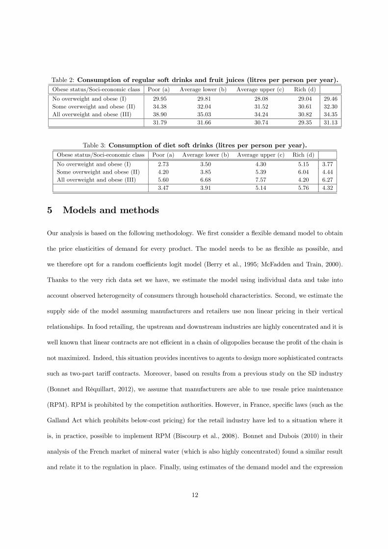
Table 2: Consumption of regular soft drinks and fruit juices (litres per person per year).Obese status/Soci-economic class Poor (a) Average lower (b) Average upper (c) Rich (d)

No overweight and obese (I) 29.95 29.81 28.08 29.04 29.46Some overweight and obese (II) 34.38 32.04 31.52 30.61 32.30All overweight and obese (III) 38.90 35.03 34.24 30.82 34.35

31.79 31.66 30.74 29.35 31.13

Table 3: Consumption of diet soft drinks (litres per person per year).Obese status/Soci-economic class Poor (a) Average lower (b) Average upper (c) Rich (d)

No overweight and obese (I) 2.73 3.50 4.30 5.15 3.77Some overweight and obese (II) 4.20 3.85 5.39 6.04 4.44All overweight and obese (III) 5.60 6.68 7.57 4.20 6.27

3.47 3.91 5.14 5.76 4.32

5 Models and methods

Our analysis is based on the following methodology. We first consider a flexible demand model to obtain

the price elasticities of demand for every product. The model needs to be as flexible as possible, and

we therefore opt for a random coefficients logit model (Berry et al., 1995; McFadden and Train, 2000).

Thanks to the very rich data set we have, we estimate the model using individual data and take into

account observed heterogeneity of consumers through household characteristics. Second, we estimate the

supply side of the model assuming manufacturers and retailers use non linear pricing in their vertical

relationships. In food retailing, the upstream and downstream industries are highly concentrated and it is

well known that linear contracts are not efficient in a chain of oligopolies because the profit of the chain is

not maximized. Indeed, this situation provides incentives to agents to design more sophisticated contracts

such as two-part tariff contracts. Moreover, based on results from a previous study on the SD industry

(Bonnet and Réquillart, 2012), we assume that manufacturers are able to use resale price maintenance

(RPM). RPM is prohibited by the competition authorities. However, in France, specific laws (such as the

Galland Act which prohibits below-cost pricing) for the retail industry have led to a situation where it

is, in practice, possible to implement RPM (Biscourp et al., 2008). Bonnet and Dubois (2010) in their

analysis of the French market of mineral water (which is also highly concentrated) found a similar result

and relate it to the regulation in place. Finally, using estimates of the demand model and the expression

12

of the pricing equilibrium, we are able to simulate the impact on consumers prices and consumption of

alternative tax policies.

5.1 The Demand Model: a random coefficients logit model

We use a random coefficients logit model to estimate the demand model and the related elasticities. The

indirect utility funtion Vijt for consumer i buying product j in period t is given by

Vijt = βb(j) + βr(j) − αipjt + ρilj + εijt

where βb(j) and βr(j) are brand and retailer fixed effects respectively that capture the (time invariant)

unobserved brand and retailer characteristics, pjt is the price of product j in period t, αi is the marginal

disutility of the price for consumer i, lj is a dummy related to an observed product characteristic (which

takes the value of 1 if product j is a diet product and 0 otherwise), ρi captures consumer i’s taste for the

diet characteristic and εijt is an unobserved error term.

We assume that αi and ρi vary across consumers. Indeed, consumers can have a different price

disutility or different tastes for the diet characteristic. We assume that distributions of αi and ρi are

independent and that the parameters have the following specification:µαiρi

¶=

µαρ

¶+ΠDi +Σvi

where Di is a set of demographics, Π is a 2×d matrix of parameters associated (with d the number of

demographics), and vi = (vαi , v

ρi )0 a 2x1 vector that captures the unobserved consumers characteristics.

Σ is a 2 × 2 diagonal matrix of parameters (σα, σρ) that measures the unobserved heterogeneity of the

consumers. We suppose that Pv(.) is a parametric distribution of vi.

We can then break down the indirect utility into a mean utility δjt = βb(j) + βr(j) + αpjt + ρlj + ξjt

where ξjt captures all unobserved product characteritics and a deviation from this mean utility µijt =

[pjt, lj ] (σαvαi +ΠαDi, σρv

ρi +ΠρDi)

0. The indirect utility is given by Vijt = δjt + µijt + εijt.

The consumer can decide not to choose one of the considered products. Thus, we introduce an outside

option that permits substitution between the considered products and a substitute. The utility of the

outside good is normalized to zero. The indirect utility of choosing the outside good is Vi0t = εi0t.

13

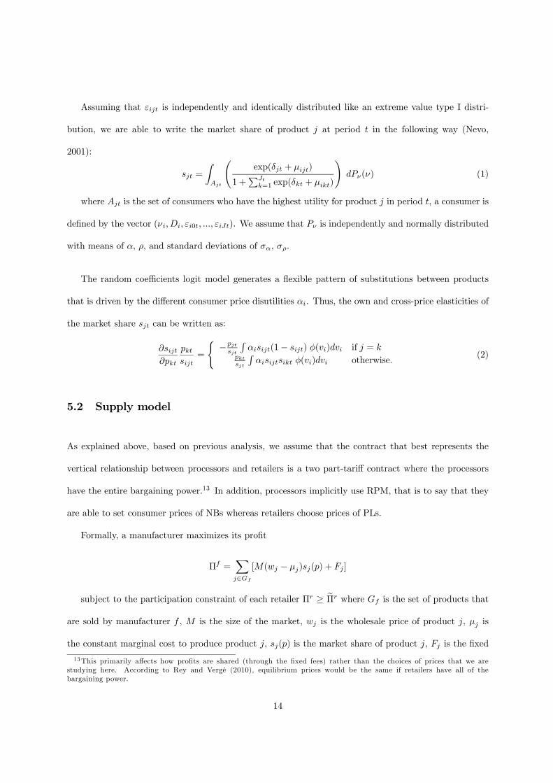
Assuming that εijt is independently and identically distributed like an extreme value type I distri-

bution, we are able to write the market share of product j at period t in the following way (Nevo,

2001):

sjt =

ZAjt

Ãexp(δjt + µijt)

1 +PJt

k=1 exp(δkt + µikt)

!dPν(ν) (1)

where Ajt is the set of consumers who have the highest utility for product j in period t, a consumer is

defined by the vector (νi,Di, εi0t, ..., εiJt). We assume that Pν is independently and normally distributed

with means of α, ρ, and standard deviations of σα, σρ.

The random coefficients logit model generates a flexible pattern of substitutions between products

that is driven by the different consumer price disutilities αi. Thus, the own and cross-price elasticities of

the market share sjt can be written as:

∂sijt∂pkt

pktsijt

=

(−pjt

sjt

Rαisijt(1− sijt) φ(vi)dvi if j = k

pktsjt

Rαisijtsikt φ(vi)dvi otherwise.

(2)

5.2 Supply model

As explained above, based on previous analysis, we assume that the contract that best represents the

vertical relationship between processors and retailers is a two part-tariff contract where the processors

have the entire bargaining power.13 In addition, processors implicitly use RPM, that is to say that they

are able to set consumer prices of NBs whereas retailers choose prices of PLs.

Formally, a manufacturer maximizes its profit

Πf =Xj∈Gf

[M(wj − µj)sj(p) + Fj ]

subject to the participation constraint of each retailer Πr ≥ eΠr where Gf is the set of products that

are sold by manufacturer f , M is the size of the market, wj is the wholesale price of product j, µj is

the constant marginal cost to produce product j, sj(p) is the market share of product j, Fj is the fixed

13This primarily affects how profits are shared (through the fixed fees) rather than the choices of prices that we arestudying here. According to Rey and Vergé (2010), equilibrium prices would be the same if retailers have all of thebargaining power.

14

fee received for product j, Πr is the profit of retailer r and eΠr is a fixed reservation utility that we cannormalize to zero without loss of generality.14

The profit of retailer r is given by:

Πr =Xj∈Sr

[M(pj − wj − cj)sj(p)− Fj ].

where Sr is the set of products that retailer r sells, and cj is the constant marginal cost to distribute

product j. In the specific case of private labels, we assume that they are sold to retailers at the marginal

cost by the producing firms.15

From the program of profit maximization and using the fact that manufacturers margins are set to

zero (wj = µj)16 , the first order conditions that determine prices of NBs are given by:

XJ

k=1(pk − µk − ck)

∂sk(p)

∂pj+ sj(p) = 0 for all j ∈ Gf (3)

whereas for PLs they are given by:

Xk∈Sr

(pk − µk − ck)∂sk(p)

∂pj+ sj(p) = 0 for all j ∈ eSr. (4)

where eSr is the set of PL products that retailer r sells. Using the above conditions and the de-mand model, we estimate price-cost margins from which we derive estimates of total marginal costs

(i.e. marginal cost of production and distribution) Cjt = pjt − γjt for each product j in period t where

γjt = pjt−µjt− cjt is the retailer’s margin for product j (remind that the manufacturer margin is set to

0).

5.3 Simulations

We simulate the impact on prices and consumption of two types of taxes, namely ad valorem tax and

excise tax. Let’s denote T = (τ , t) with τ = (τ1, .., τ j , .., τJ) and t = (t1, .., tj , .., tJ) the tax system where

14As a product is a combination of a brand and a retailer, one can define a fixed fee for each product. It is interpreted asthe fixed fee paid by a given retailer (if positive) to a given manufacturer.15A retailer defines the characteristics of its own private label. It then delegates the production of this product to a

manufacturer. In this process the retailer organizes competition among producers for a given product. This competition isinterpreted to be a price competition with a homogenous product that leads to a selling price that is equal to the marginalcosts. For additional information on private labels, refer to Bergès-Sennou et al. (2004).16Fixed fees are thus the tool allowing profit sharing between manufacturers and retailers.

15

τ is the vector of ad valorem tax and t is the vector of excise tax. Initially, the vector τ is the vector of

VAT and the vector t is nil, we thus have T0 = (τ0, 0). Imposing a tax on soft drinks using ad valorem

and excise tax leads to the tax system T1 = (τ1, t1).

The simulation tool uses the estimated marginal costs from the supply model as well as the other

estimated structural parameters. We denote Ct = (C1t, .., Cjt, .., CJt) the vector of marginal costs for all

products present at period t, where Cjt is given by Cjt = pjt − γjt . When the tax changes from T0 to

T1 the new price equilibria is deduced from the following program:

min{p∗jt}j=1,..,J

kp∗t − eγt (p∗t )− Ct − t1k (5)

where k.k is the Euclidean norm in RJ . The vector eγt (p∗t ) is the retail margins for the best supply modelcontracts and comes from the following profit maximisation program of manufacturers for national brands

max{pk}k∈Gf

JXj=1

(1 + τ01 + τ1

pj − wj − cj)sj(p) (6)

and the following profit maximization program of retailers for private labels

max{pk}k∈Sr

Xj∈Sr

(1 + τ01 + τ1

pj − µj − cj)sj(p) +X

j∈Sr\Sr

(1 + τ01 + τ1

p∗j − µj − cj)sj(p∗).17 (7)

6 Results on demand and vertical relationships

We estimated the demand model using individual data. We randomly choose 100,000 observations among

the 450,000 we have.18 We used the simulated maximum likelihood method as in Revelt and Train (1998).

This method relies on the assumption that all product characteristics Xjt = (pjt, lj) are independant

of the error term εijt. However, assuming εijt = ξjt+ eijt where ξjt is a product-specific error term

varying across periods and eijt is an individual specific error term, the independance assumption cannot

be hold if unobserved factors included in ξjt (and hence in εijt) as promotions, displays, advertising are

17We obtain expressions (6) and (7) assuming that each marginal cost component is taxed to the same rate than thepresent ad valorem tax of food products. We are aware that this assumption might not be always true but the lack of dataon the composition of the marginal cost of each product requires to have such assumption.18Due to constraints on computers, we are not able to estimate the demand model using the whole sample. The sample

used is representative of the whole sample over products and periods.

16

correlated with observed characteritics Xjt. For instance, we do not know the amount of advertising

that firms invest each month for their brand. This effect is thus included in the error term because

advertising might play a role in the choice of SD by households. As advertising is an appreciable share of

SD production costs, it is obviously correlated with prices. To solve the problem that omitted product

characteristics might be correlated with prices, we use a control function approach as in Petrin and Train

(2010). We then regress prices on instrumental variables, that is input prices, as well as product and

time fixed effects:

pjt =Wjtγ + δb(j) + δr(j) + µlj + ηjt

where Wjt is a vector of input price variables, γ the vector of parameters associated and ηjt is an

error term that captures the remaining unobserved variations in prices. The estimated error term bηjtof the first stage includes some omitted variables as advertising variations, promotions. Introducing this

term in the mean utility of consumers δjt allows to capture unobserved product characteristics varying

across time. Prices are now uncorrelated with the new error term ξjt + εjht − λbηjt. We then writeδjt= βb(j)+βr(j)+αpjt+ρl j+ξjt+λbηjt

where λ is the estimated parameter associated with the estimated error term of the first stage.

In practice, we use input price indexes of wages, plastic, aluminium, sugar and gasoline as it is

unlikely that input prices are correlated with unobserved determinants of demand for SDs.19 The SD

industry only represents a very small share of the demand for those inputs which justify the absence of

correlation between input prices and unobserved determinants of the demand for SDs. These variables are

interacted with the manufacturers dummies or private label/national brand dummies because we expect

that manufacturers obtain different prices from suppliers for raw materials and that some characteristics

of the inputs (e.g. quality of plastic) depend on the manufacturers.

We estimated two models (Table 4). Model 1 is the demand model without controlling for the

endogeneity problem of prices whereas model 2 controls for it.20 First, the coefficient of the error term19These indexes are from the French National Institute for Statistics and Economic Studies.20Models were estimated using 100 draws for the parametric distribution that represents the unobserved consumer char-

acteristics.

17

is positive and significant. It means that the unobserved part explaining prices is positively correlated

with the choice of the alternative and justify the need to control for endogeneity problem. Comparison

of results from model 1 and 2 reveals that the estimates of the parameters of the model are robust to

instrumentation.

In both models we introduced some household heterogeneity in the price sensitivity or in the taste

for the diet characteristic. The price sensitivity which is reported is for a ’rich’ household without

any individual obese or overweight (income class ’d’, obesity class ’I’). Then the coefficient of interaction

between price and any other class of obesity or income indicates how the price sensitivity is affected by the

corresponding household characteristics. The sensitivity to the diet characteristics indicate the preference

of consumers for diet product compared to the regular product. We also analyze the interactions with

income class or obesity class. However, to minimize the number of coefficients to estimate, rather than

using dummies we use the percentage of individuals that are overweight or obese in the households and

we use the socio-economic variable for income. On average, the price has a significant and negative impact

on utility. Consumers are more sensitive to the price variations of PLs than to NBs. This is consistent

with the idea that consumers might have more loyalty with respect to NBs than to PLs. Households with

overweight or obese individuals are slightly less sensitive to price than households with no overweight or

obese individuals. The proportion of overweight and obese individuals in the household has no impact

on this result. We also find that households from the richest class are more sensitive to price. However,

as is the case for the obesity class, the differences in price sensitivity are rather small. They are much

smaller than the difference in price sensitivity to PLs versus NBs. Results suggest that households prefer

regular products than diet products, since the mean coefficient is negative and the standard deviation

quite low. However, the preference decreases with the percentage of obese individuals in the household

and with the class of income. This result might be related to the information campaigns that recommend

to limit the consumption of added sugar and in particular to limit SD consumption. It is consistent with

the idea that highly educated people (assuming a correlation between the level of education and income)

are more receptive to these messages.

18

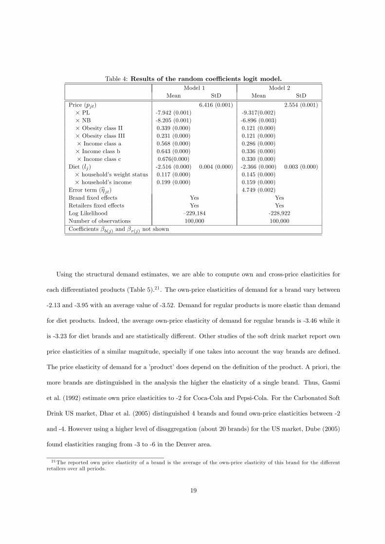
Table 4: Results of the random coefficients logit model.Model 1 Model 2

Mean StD Mean StD

Price (pjt) 6.416 (0.001) 2.554 (0.001)× PL -7.942 (0.001) -9.317(0.002)× NB -8.205 (0.001) -6.896 (0.003)× Obesity class II 0.339 (0.000) 0.121 (0.000)× Obesity class III 0.231 (0.000) 0.121 (0.000)× Income class a 0.568 (0.000) 0.286 (0.000)× Income class b 0.643 (0.000) 0.336 (0.000)× Income class c 0.676(0.000) 0.330 (0.000)

Diet (lj) -2.516 (0.000) 0.004 (0.000) -2.366 (0.000) 0.003 (0.000)× household’s weight status 0.117 (0.000) 0.145 (0.000)× household’s income 0.199 (0.000) 0.159 (0.000)

Error term (bηjt) 4.749 (0.002)Brand fixed effects Yes YesRetailers fixed effects Yes YesLog Likelihood —229,184 -228,922Number of observations 100,000 100,000Coefficients βb(j) and βr(j) not shown

Using the structural demand estimates, we are able to compute own and cross-price elasticities for

each differentiated products (Table 5).21. The own-price elasticities of demand for a brand vary between

-2.13 and -3.95 with an average value of -3.52. Demand for regular products is more elastic than demand

for diet products. Indeed, the average own-price elasticity of demand for regular brands is -3.46 while it

is -3.23 for diet brands and are statistically different. Other studies of the soft drink market report own

price elasticities of a similar magnitude, specially if one takes into account the way brands are defined.

The price elasticity of demand for a ’product’ does depend on the definition of the product. A priori, the

more brands are distinguished in the analysis the higher the elasticity of a single brand. Thus, Gasmi

et al. (1992) estimate own price elasticities to -2 for Coca-Cola and Pepsi-Cola. For the Carbonated Soft

Drink US market, Dhar et al. (2005) distinguished 4 brands and found own-price elasticities between -2

and -4. However using a higher level of disaggregation (about 20 brands) for the US market, Dube (2005)

found elasticities ranging from -3 to -6 in the Denver area.

21The reported own price elasticity of a brand is the average of the own-price elasticity of this brand for the differentretailers over all periods.

19

Table 5: Average own-price elasticities of the brandsBrands Characteristic Own price Elasticity Brands Characteristic Own price Elasticity

B1 R -3.25 (0.06) B10 R -3.71 (0.09)B2 D -3.34 (0.06) B11 R -3.81 (0.05)B3 R -3.66 (0.02) B12 R -3.65 (0.07)B4 D -3.75 (0.04) B13 R -3.81 (0.03)B5 R -3.90 (0.04) B14 R -2.75 (0.07)B6 D -3.91 (0.04) B15 R -3.65 (0.16)B7 R -3.88 (0.04) B16 R -3.10 (0.06)B8 R -3.95 (0.02) B17 D -2.13 (0.05)B9 D -3.80 (0.02)

R: Regular, D: Diet

Price-cost margins are 47.2% of the consumer price, on average. The margins are relatively heteroge-

neous across brands (Table 15 in the appendix). The average price-cost margins for the PLs (42.0%) are

significantly lower than those for the NBs (50.1%). The price-cost margins for diet products (52.5%) are

significantly higher than those for regular products (45.4%). The price-cost margins do not differ across

retailers. The estimated marginal cost is 0.39€/litre on average. The average marginal cost of the PLs

(0.25€/litre) is lower than that of the NBs (0.44€/litre).

7 Impact of taxation

We evaluate the impact of taxes taking into account consumer substitution patterns and strategic pricing

of firms. We simulate three policy scenarios to determine the impact of alternative ways of taxation. In

order to make comparable the scenarios, taxes are designed in such a way that in absence of consumers

and firms reaction, the tax revenues are the same in the three cases. In scenario 1 we consider an uniform

ad valorem tax on regular soft drinks. We assume that the VAT of regular products goes up to 19.6%

instead of the 5.5%’s.22 In scenario 2, we base the ad valorem tax on the sugar content of products. To

22The VAT of food products that prevails in France is 5.5% except for sweets and some chocolate products which are atthe standard rate of 19.6%. In 2008, some French delegates proposed to increase VAT of regular SDs to the standard rateof 19.6%. As explained above, since January 2012, an excise tax of 0.0716 €/litre is levied on all SDs whatever they areregular or diet.

20

get the same ex ante revenues as those in scenario 1, a 0.14% tax per gram of sugar per litre is applied.

The final VAT now varies from 16.8% to 21.4% depending on the sugar content of products. In scenario

3, we design an excise tax based on the sugar content of products which is added to the current VAT tax.

Ex ante revenue neutrality leads to design a 0.09 cents of euros per gram of sugar per litre of product.

The excise tax ranges from 7.4 cents to 10.5 cents per litre of regular soft drink.

7.1 Impact on prices

We use (5) to compute the after tax equilibria. It should be acknowledged that the model integrates the

brand portfolio of the manufacturers as well as the assortment of products sold by the retailers. However

due to resale price maintenance the strategic choice of prices is made by manufacturers for NBs whereas

it is retailers who choose PLs prices. Thus a manufacturer chooses his pricing policy for the whole set of

products he sells, internalizing substitutions among his own set of products. We find that firms behave

differently depending on the type of taxation they face (Table 6). When facing an increase in the ad

valorem tax, they transfer to the consumers less than the tax (scenarios 1 and 2). According to our

results, firms pass on to the consumers from 60 to 90% of the tax increase depending on the brand. Thus,

the consumer price integrating strategic pricing by firms is lower than the consumer price assuming a full

transmission of the amount of the tax on to consumers (we refer to this latter case as ’passive pricing’).

The comparison of scenarios 1 and 2 suggests that the pass-through of the tax is brand specific as

the ranking of the pass-through is similar in both cases. PL products are mechanically less affected by

an ad valorem tax as their prices are significantly lower than those of NB products. Note also that the

prices of diet products change even if those products do not support any additional tax. Firms behave

aggressively in the sense that the prices of diet products are reduced. As a consequence, diet products

gain significant market shares. When facing an excise tax (scenario 3), firms transfer more than the tax to

final consumers. The consumer prices increase by 107 to 133% of the excise tax depending on the brand.

The pass-through rates of PLs are significantly lower than those of NBs. An excise tax penalizes more

21

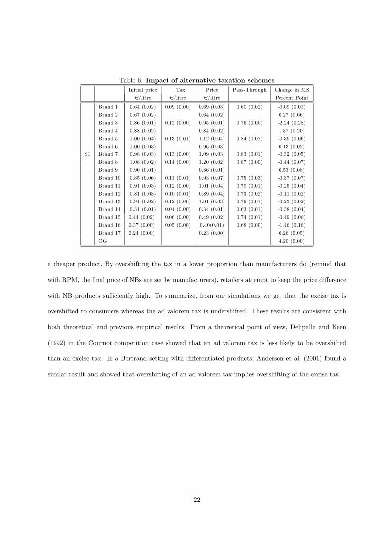
Table 6: Impact of alternative taxation schemesInitial price Tax Price Pass-Through Change in MS

€/litre €/litre €/litre Percent Point

Brand 1 0.64 (0.02) 0.09 (0.00) 0.69 (0.03) 0.60 (0.02) -0.09 (0.01)

Brand 2 0.67 (0.02) 0.64 (0.02) 0.27 (0.06)

Brand 3 0.86 (0.01) 0.12 (0.00) 0.95 (0.01) 0.76 (0.00) -2.24 (0.28)

Brand 4 0.88 (0.02) 0.84 (0.02) 1.37 (0.20)

Brand 5 1.00 (0.04) 0.13 (0.01) 1.12 (0.04) 0.84 (0.02) -0.39 (0.06)

Brand 6 1.00 (0.03) 0.96 (0.03) 0.13 (0.02)

S1 Brand 7 0.98 (0.03) 0.13 (0.00) 1.09 (0.03) 0.83 (0.01) -0.32 (0.05)

Brand 8 1.08 (0.02) 0.14 (0.00) 1.20 (0.02) 0.87 (0.00) -0.44 (0.07)

Brand 9 0.90 (0.01) 0.86 (0.01) 0.53 (0.08)

Brand 10 0.85 (0.06) 0.11 (0.01) 0.93 (0.07) 0.75 (0.03) -0.37 (0.07)

Brand 11 0.91 (0.03) 0.12 (0.00) 1.01 (0.04) 0.79 (0.01) -0.25 (0.04)

Brand 12 0.81 (0.03) 0.10 (0.01) 0.89 (0.04) 0.73 (0.02) -0.11 (0.02)

Brand 13 0.91 (0.02) 0.12 (0.00) 1.01 (0.03) 0.79 (0.01) -0.23 (0.02)

Brand 14 0.31 (0.01) 0.04 (0.00) 0.34 (0.01) 0.63 (0.01) -0.38 (0.04)

Brand 15 0.44 (0.02) 0.06 (0.00) 0.49 (0.02) 0.74 (0.01) -0.49 (0.06)

Brand 16 0.37 (0.00) 0.05 (0.00) 0.40(0.01) 0.68 (0.00) -1.46 (0.16)

Brand 17 0.24 (0.00) 0.23 (0.00) 0.26 (0.05)

OG 4.20 (0.00)

a cheaper product. By overshifting the tax in a lower proportion than manufacturers do (remind that

with RPM, the final price of NBs are set by manufacturers), retailers attempt to keep the price difference

with NB products sufficiently high. To summarize, from our simulations we get that the excise tax is

overshifted to consumers whereas the ad valorem tax is undershifted. These results are consistent with

both theoretical and previous empirical results. From a theoretical point of view, Delipalla and Keen

(1992) in the Cournot competition case showed that an ad valorem tax is less likely to be overshifted

than an excise tax. In a Bertrand setting with differentiated products, Anderson et al. (2001) found a

similar result and showed that overshifting of an ad valorem tax implies overshifting of the excise tax.

22

Table 6: Impact of alternative taxation schemes (continued)Initial price Tax Price Pass-Through Change in MS

€/litre €/litre €/litre Percent Point

Brand 1 0.64 (0.02) 0.10 (0.00) 0.70 (0.03) 0.64 (0.02) -0.11 (0.01)

Brand 2 0.67 (0.02) 0.64 (0.02) 0.27 (0.06)

Brand 3 0.86 (0.01) 0.10 (0.00) 0.96 (0.01) 0.78 (0.00) -2.48 (0.30)

Brand 4 0.88 (0.02) 0.84 (0.02) 1.37 (0.20)

Brand 5 1.00 (0.04) 0.06 (0.00) 1.07 (0.04) 0.68 (0.02) -0.16 (0.02)

Brand 6 1.00 (0.03) .96 (0.03) 0.13 (0.02)

S2 Brand 7 0.98 (0.03) 0.08 (0.00) 1.07 (0.03) 0.78 (0.01) -0.26(0.04)

Brand 8 1.08 (0.02) 0.10 (0.01) 1.21 (0.02) 0.89 (0.00) -0.48 (0.07)

Brand 9 0.90 (0.01) 0.86 (0.01) 0.53 (0.08)

Brand 10 0.85 (0.06) 0.09 (0.00) 0.92 (0.06) 0.72 (0.03) -0.36 (0.07)

Brand 11 0.91 (0.03) 0.09 (0.00) 1.01 (0.04) 0.79 (0.01) -0.26 (0.04)

Brand 12 0.81 (0.03) 0.09 (0.01) 0.89 (0.04) 0.72 (0.02) -0.11 (0.02)

Brand 13 0.91 (0.02) 0.10 (0.00) 1.03 (0.03) 0.83 (0.01) -0.28 (0.03)

Brand 14 0.31 (0.01) 0.10 (0.00) 0.34 (0.01) 0.64 (0.01) -0.45 (0.05)

Brand 15 0.44 (0.02) 0.07 (0.00) 0.48 (0.02) 0.72 (0.01) -0.36 (0.04)

Brand 16 0.37 (0.00) 0.10 (0.00) 0.40 (0.01) 0.68 (0.00) -1.55(0.17)

Brand 17 0.24 (0.00) 0.23 (0.00) 0.26 (0.05)

OG 4.22 (0.00)

Brand 1 0.64 (0.02) 0.09 (0.00) 0.77 (0.02) 1.28 (0.00) -0.20 (0.05)

Brand 2 0.67 (0.02) 0.65 (0.02) 0.30 (0.08)

Brand 3 0.86 (0.01) 0.12 (0.00) 0.99 (0.01) 1.34 (0.00) -2.91 (0.39)

Brand 4 0.88 (0.02) 0.86 (0.02) 1.44 (0.22)

Brand 5 1.00 (0.04) 0.09 (0.00) 1.08 (0.04) 1.25 (0.01) -0.14 (0.03)

Brand 6 1.00 (0.03) 0.98 (0.03) 0.13 (0.02)

S3 Brand 7 0.98 (0.03) 0.12 (0.00) 1.09 (0.03) 1.33 (0.01) -0.24 (0.02)

Brand 8 1.08 (0.02) 0.15 (0.01) 1.21 (0.02) 1.40 (0.00) -0.38 (0.04)

Brand 9 0.90 (0.01) 0.88 (0.01) 0.56 (0.09)

Brand 10 0.85 (0.06) 0.10 (0.00) 0.96 (0.06) 1.30 (0.01) -0.40 (0.05)

Brand 11 0.91 (0.03) 0.12 (0.00) 1.04 (0.03) 1.34 (0.01) -0.28 (0.03)

Brand 12 0.81 (0.03) 0.11 (0.01) 0.93 (0.04) 1.30 (0.01) -0.14 (0.03)

Brand 13 0.91 (0.02) 0.14 (0.00) 1.05 (0.02) 1.37 (0.01) -0.30 (0.03)

Brand 14 0.31 (0.01) 0.05 (0.00) 0.42 (0.01) 1.07 (0.00) -1.68 (0.31)

Brand 15 0.44 (0.02) 0.05 (0.00) 0.52 (0.02) 1.07 (0.00) -0.76(0.16)

Brand 16 0.37 (0.00) 0.05 (0.00) 0.47 (0.00) 1.07 (0.00) -3.66 (0.48)

Brand 17 0.24 (0.00) 0.23 (0.00) 0.43 (0.10)

OG 8.18 (0.00)

From an empirical point of view, this result is also consistent with the analysis of Campa and Goldberg

(2006) who found that pass-through rates in the food industry in France are larger than one (1.41).

Besley and Rosen (1999) found that the US soft drink industry had overshifted tax changes. Delipalla

and O’Donnell (2001) using data from the European cigarette market studied how firms react to different

taxation on the European cigarette industry. They found that in 10 countries (over 12) the price effect

of an excise tax was larger than the price effect of an ad valorem tax. Finally, Griffith et al. (2010) in a

23

simulation exercise of the impact of butter taxation in the UK, also found overshifting of an excise tax

and undershifting of an ad valorem tax.

7.2 Impact on market shares and consumption

The excise tax has a larger impact on SD consumption than ad valorem tax. This is the consequence of

producers’ behavior who overshift the excise tax whereas they undershift the ad valorem tax. With ad

valorem taxation the market shares of regular PLs are less affected than those of regular NBs. For example

in scenario 1, they decrease by 18% on average whereas the market shares of regular NBs decrease by

23% on average. On the contrary, with an excise tax it is the market shares of regular NBs which are

less affected (-25% and -48% on average for NBs and PLs respectively). This directly relates to the price

impact of taxes. Ad valorem taxes affect less the cheaper products whereas it is the contrary with excise

taxes.

When the ad valorem tax depends on the sugar content (scenario 2), the market shares of highly

sweetened brands are more affected. However the overall impact on SD consumption of the ad valorem

tax does not depend on the design of the tax. Thus, the aggregate market share of regular products

decreases by 6.8 points in both scenarios 1 and 2 (Table 6) . This decrease in consumption is compensated

by an increase in the market share of diet products (+2.6 points) and the outside good (4.2 points).23

With an excise tax, the impact on the aggregate market share of regular products is larger (-11 points).

The decrease is compensated by an increase of the market shares of diet products (+2.8 points) and

mainly an increase of the market share of the outside good (+8.2 points). 24

Under passive pricing, that is assuming than 100% of the tax is transmitted to the consumers, the three

different schemes of taxation have a similar aggregate impact on the consumption of regular products

which would be reduced by approximately 4.5 litres to 5 litres per person per year (Table 7). This is

no longer the case when taking into account the strategic pricing of firms. With an ad valorem tax the23 In this modeling, the global size of the market does not change. Any reduction in the consumption of one product is

compensated by the increase in consumption of some other goods including the outside good.24 It should be noted that in these simulations, we assume that the price of the outside option does not change. As the

outside option is mostly composed of fruit juices, it is likely that those products would not be taxed as their consumptionis recommended by health authorities (as being ’fruits’) and because they do not contain ’added sugar’.

24

Table 7: Changes in the consumption of SD (per person per year)Initial values Scenario 1 Scenario 2 Scenario 3

Passive Strategic Passive Strategic Passive Strategic

Consumption Soft drink (in litres)

Regular products 13.55 -4.45 -3.72 -4.47 -3.73 -5.11 -6.07

Diet products 4.33 0.95 1.40 0.95 1.40 0.97 1.56

Consumption of added sugar (in grams) 1666 -419 -352 -427 -360 -499 -629

consumption of regular SDs drops by approximately 3.7 litres per person per year whereas it drops by

more than 6 litres per person per year with the excise tax. This result strongly supports the need for

empirical analysis to integrate price behavior of firms. With ad valorem tax, strategic pricing by firms

tends to lower the impact on consumption as firms do not fully transmit the tax to consumers. On the

contrary, with an excise tax, strategic pricing by firms tends to increase the impact on consumption as

firms overshift the tax.

7.3 Which tax is the most efficient?

There are different ways to evaluate the efficiency of the tax. A first criteria could be the impact on

consumption of added sugar as the objective of such taxation might be to limit added sugar consumption

as recommended by health authorities (for example the French Programme National Nutrition Santé

recommends to decrease the consumption of added sugar by 25%). From this point of view, it is the

excise tax based on the sugar content which has the highest impact on sugar consumption (Table 7).25

This is the consequence of both a better targeting of the tax and strategic pricing by firms which increases

the impact on consumers. The tax is better targeted as the larger the sugar content the larger the tax.

The ad valorem tax based on sugar content adapts the rate of taxation to the sugar content but it failed

to well target low priced products (PLs) as it is an ad valorem tax. Griffith et al. (2010) find a similar

25 It should be noted that the overall impact on sugar consumption is lower. Thus, if diet products do not contain sugar,it is not the case of the outside good. The outside good is mainly composed of fruit juice which naturally contains sugarbut do not contain added sugar (except for nectars which integrate a relatively small amount of added sugar). On average,according to Observatoire de la Qualite de l’Alimentation (2010) fruit juice contains about 100g/l of sugar. In that case thenet change in sugar consumption of taxation would be 120, 128 and 178 g for scenario 1, 2 and 3 respectively. If from anhealth point of view the relevant criteria is sugar consumption then the overall impact of the tax is lower. The excise taxis still the most efficient but the difference with ad valorem taxation is smaller.

25

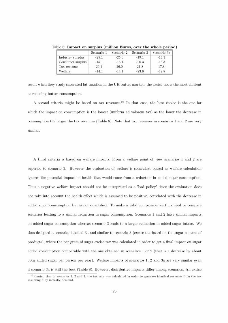
Table 8: Impact on surplus (million Euros, over the whole period)Scenario 1 Scenario 2 Scenario 3 Scenario 3a

Industry surplus -25.1 -25.0 -19.1 -14.3Consumer surplus -15.1 -15.1 -26.3 -16.3Tax revenue 26.1 26.0 21.8 17.8Welfare -14.1 -14.1 -23.6 -12.8

result when they study saturated fat taxation in the UK butter market: the excise tax is the most efficient

at reducing butter consumption.

A second criteria might be based on tax revenues.26 In that case, the best choice is the one for

which the impact on consumption is the lowest (uniform ad valorem tax) as the lower the decrease in

consumption the larger the tax revenues (Table 8). Note that tax revenues in scenarios 1 and 2 are very

similar.

A third criteria is based on welfare impacts. From a welfare point of view scenarios 1 and 2 are

superior to scenario 3. However the evaluation of welfare is somewhat biased as welfare calculation

ignores the potential impact on health that would come from a reduction in added sugar consumption.

Thus a negative welfare impact should not be interpreted as a ’bad policy’ since the evaluation does

not take into account the health effect which is assumed to be positive, correlated with the decrease in

added sugar consumption but is not quantified. To make a valid comparison we thus need to compare

scenarios leading to a similar reduction in sugar consumption. Scenarios 1 and 2 have similar impacts

on added-sugar consumption whereas scenario 3 leads to a larger reduction in added-sugar intake. We

thus designed a scenario, labelled 3a and similar to scenario 3 (excise tax based on the sugar content of

products), where the per gram of sugar excise tax was calculated in order to get a final impact on sugar

added consumption comparable with the one obtained in scenarios 1 or 2 (that is a decrease by about

360g added sugar per person per year). Welfare impacts of scenarios 1, 2 and 3a are very similar even

if scenario 3a is still the best (Table 8). However, distributive impacts differ among scenarios. An excise

26Remind that in scenarios 1, 2 and 3, the tax rate was calculated in order to generate identical revenues from the taxassuming fully inelastic demand.

26

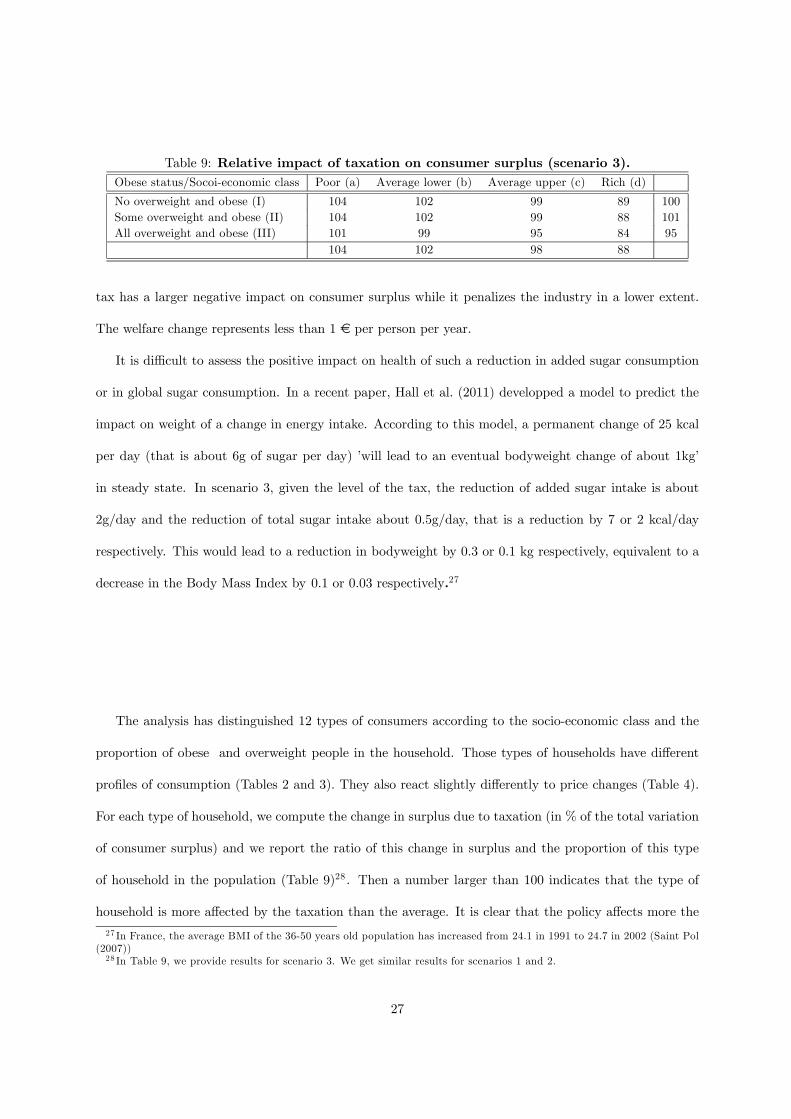
Table 9: Relative impact of taxation on consumer surplus (scenario 3).Obese status/Socoi-economic class Poor (a) Average lower (b) Average upper (c) Rich (d)

No overweight and obese (I) 104 102 99 89 100Some overweight and obese (II) 104 102 99 88 101All overweight and obese (III) 101 99 95 84 95

104 102 98 88

tax has a larger negative impact on consumer surplus while it penalizes the industry in a lower extent.

The welfare change represents less than 1 € per person per year.

It is difficult to assess the positive impact on health of such a reduction in added sugar consumption

or in global sugar consumption. In a recent paper, Hall et al. (2011) developped a model to predict the

impact on weight of a change in energy intake. According to this model, a permanent change of 25 kcal

per day (that is about 6g of sugar per day) ’will lead to an eventual bodyweight change of about 1kg’

in steady state. In scenario 3, given the level of the tax, the reduction of added sugar intake is about

2g/day and the reduction of total sugar intake about 0.5g/day, that is a reduction by 7 or 2 kcal/day

respectively. This would lead to a reduction in bodyweight by 0.3 or 0.1 kg respectively, equivalent to a

decrease in the Body Mass Index by 0.1 or 0.03 respectively.27

The analysis has distinguished 12 types of consumers according to the socio-economic class and the

proportion of obese and overweight people in the household. Those types of households have different

profiles of consumption (Tables 2 and 3). They also react slightly differently to price changes (Table 4).

For each type of household, we compute the change in surplus due to taxation (in % of the total variation

of consumer surplus) and we report the ratio of this change in surplus and the proportion of this type

of household in the population (Table 9)28 . Then a number larger than 100 indicates that the type of

household is more affected by the taxation than the average. It is clear that the policy affects more the

27 In France, the average BMI of the 36-50 years old population has increased from 24.1 in 1991 to 24.7 in 2002 (Saint Pol(2007))28 In Table 9, we provide results for scenario 3. We get similar results for scenarios 1 and 2.

27

poor than the rich and is thus regressive. However, with respect to the obesity status, households with

all individual obese or overweight are less affected. This is because those households consume more diet

products than the average.

8 Conclusion

This paper provides a general methodology for assessing impacts of tax policies on the food consumption

taking into account pricing strategies of both manufacturers and retailers in the food chain. We analyze

the impact of alternative ways for soft drink taxation. Using the recent development of empirical industrial

organization, we have estimated a very flexible demand model, a random coefficients logit model, and as

stated by previous work, we assume that the most likely supply model is the one where manufacturers

and retailers use two-part tariffs contracts with resale price maintenance and where private labels play

no role in manufacturer/retailer relationships, meaning that manufacturers have a large market power.

Using this model, we have simulated the impact on consumer prices of alternative tax scenarios taking

into account the strategic choice of prices by firms. From the demand model, we found that consumers are

more sensitive to the price variations of PLs than to NBs. We also found that households prefer regular

products than diet products. But this preference decreases with the percentage of obese individuals in the

household. It also decreases with income. Because we distinguished a large number of brands, we find that

demand are price elastic (about -3.5). With respect to taxation, we found that firms behave differently

when facing an ad valorem tax or an excise tax. Excise tax is overshifted to consumer prices while ad

valorem tax is undershifted to consumer prices. This result is in line with the findings of the theoretical

literature. It is also in line with what have been analysed on the cigarette industry. We showed that

ignoring strategic pricing would lead to overestimate the change in regular products consumption by 20%

when firms are facing an ad valorem tax while it would lead to underestimate the change in consumption

by about 15% when firms are facing an excise tax. We thus conclude that when analyzing food price

policies, it is needed to take into account strategic pricing. This is an important point as it is frequently

argued that assuming passive pricing provides an upper bound of the impact of the policy (e.g. Allais

28

et al., 2010, p.238). This statement is true only if producers transmit less than the tax. From our results,

we also conclude that an excise tax based on the sugar content is the most efficient way to limit soft drink

consumption. It is also the tax which, for a given target of reduction in the consumption of added sugar,

is the least costly in terms of welfare. Evaluating the impact of the tax on health outcomes is difficult

and it is thus not possible to evaluate precisely the benefit of taxation in term of health improvment. The

impact of the tax on SD consumption is significant. However, it should be acknowledged that the impact

of the tax on the consumption of sugar is small. This is mainly for two reasons. First, in France, SD

consumption is lower than in other countries and we consider here only a part of the consumption that is

at home consumption. Second, the decrease in consumption of sugar sweetened SD is partly compensated

by an increase in the consumption of fruit juice which also contains sugar. This substitution effect limits

the decrease in total sugar consumption. On the other hand, the decrease in added sugar does not suffer

from this substitutiuon effect as most of the sugar in fruit juice are ’native’ rather than added. Overall,

the welfare cost is small, about € 1 per person per year.

Our analysis suffers from some limits. First, simulations assume that the price of the outside option

is unchanged which means that those products are not taxed and that producers of the outside option

do not strategically react. A significant part of the outside option is composed of fruit juice which do not

contain any added sugar. It is unlikely that those products would be taxed because their consumption

is recommended as being ’fruits’. Moreover if the tax is put in place through added sugar taxation they

would not be concerned. However, the assumption of passive pricing remains. Even if this segment of

production is much less concentrated than the production of soft drinks, meaning that producers have

less market power, it remains true that retailers might adapt prices of these products. Second, in a longer

run, producers might also adapt the composition of their products to taxation. For example, if sweetened

products are taxed according to their sugar content, this might provide incentives to producers to lower

the sugar content of their product in order to avoid or limit the impact of taxes. Such a reaction would go

in the right direction as long as the drop in added sugar per litre is not overcompensated by an increase

in consumption in response to lower taxes (which are based on the sugar content). Dealing with such

29

an issue would require additional information on the composition of products, as well as integrating a

choice of quality by producers. An issue which as far as we know is not integrated in the empirical models

of industrial organization and then in analysis of public health policies. Third, we use a static demand

model that does not take into account addiction issues in the consumption. In that case, the impact

of the tax might be higher as limiting the consumption today might induce a stronger reduction in the

future. Finally, we neglect the fact that the tax might be perceived by some consumers as a health tool.

In that case, the tax might convey some information and might thus modify the consumer behavior. As

in the previous case, this would reinforce the impact of the tax on consumption.

Acknowledgements

We thank Marine Spiteri for her help to collect information of sugar content in the Soft Drink In-

dustry, Olivier de Mouzon for his programming work and Philippe de Donder for helpful comments.

We also thank participants at the ALISS-INRA seminar, the internal IFS seminar at London, the Nine-

teenth European Workshop on Econometrics and Health Economics in Lausanne, and the first joined

EAAE/AAEA seminar in Freising. Any remaining errors are ours.

References

Adda, J., Cornaglia, F., 2006. Taxes, cigarette consumption, and smoking intensity. American Economic

Review 96(4), 1013—1028.

Allais, O., Bertail, P., Nichele, V., 2010. The effects of a fat tax on french households’ purchases: a

nutritional approach. American Journal of Agricultural Economics 92, 228—245.

Anderson, S. P., de Palma, A., Kreider, B., 2001. Tax incidence in differentiated product oligopoly.

Journal of Public Economics 81 (2), 173 — 192.

Barnett, P., Keeler, T., Hu, T., 1995. Oligopoly structure and the incidence of cigarette excise taxes.

Journal of Public Economics 57, 457—470.

30

Becker, G. S., Murphy, K. M., 1988. A theory of rational addiction. Journal of Political Economy 96 (4),

675.

Bergès-Sennou, F., Bontems, P., Réquillart, V., 2004. Economics of private labels: A survey of literature.

Journal of Agricultural and Food Industrial Organization Num 2, Article 3.

Berry, S., Levinsohn, J., Pakes, A., 1995. Automobile prices in market equilibrium. Econometrica 63,

841—890.

Berto Villas-Boas, S., 2007. Vertical relationships between manufacturers and retailers: Inference with

limited data. Review of Economic Studies 74, 625—652.

Besley, T., Rosen, H., 1999. Sales taxes and prices: an empirical analysis. National Tax Journal 52(2),

157—178.

Bettendorf, L., Verboven, F., 2000. Incomplete transmission of coffee bean prices: evidence from the

Netherlands. European Review of Agricultural Economics 27(1), 1—16.

Biscourp, P., Boutin, X., Vergé, T., 2008. The effects of retail regulation on prices : evidence from French

data. INSEE-DESE Working Paper G2008/02, Paris France.

Bonnet, C., Dubois, P., 2010. Inference on vertical contracts between manufacturers and retailers allowing

for non linear pricing and resale price maintenance. Rand Journal of Economics 41(1), 139—164.

Bonnet, C., Dubois, P., Klapper, D., Villas-Boas, S., 2012. Empirical evidence on the role of nonlinear

wholesale pricing and vertical restraints on cost pass-through. Review of Economics and Statistics

Forthcoming.

Bonnet, C., Requillart, V., 2011. Does the EU sugar policy reform increase added sugar consumption?

an empirical evidence on the soft drink market. Health Economics 20(9), 1012—1024.

Bonnet, C., Réquillart, V., 2012. Sugar policy reform, tax policy and price transmission in the soft drink

market. WP TRANSFOP, 4, www.transfop.eu.

31

Campa, J. M., Goldberg, L. S., 2006. Pass through of exchange rates to consumption prices: What has

changed and why? In International Financial Issues in the Pacific Rim: Global Imbalances, Financial

Liberalization and Exchange Rate Policy. NBER and University of Chicago Press.

Cremer, H., De Donder, P., Maldonado, D., Pestieau, P., 2012. Taxing sin goods and subsidizing health

care. Scandinavian Journal of Economics 114 (1), 101 — 123.

Cutler, D. M., Glaeser, E. L., Shapiro, J. M., 2003. Why have americans become more obese? Journal of

Economic Perspectives 17(3), 93—118.

Dallongeville, J., Dauchet, L., de Mouzon, O., L-G., S., Requillart, V., 2011. Increasing fruit and vegetable

consumption: A cost-benefit analysis of public policies. European Journal of Public Health 21(1), 69—

73.

Delipalla, S., Keen, M., 1992. The comparison between ad valorem and specific taxation under imperfect

competition. Journal of Public Economics 49 (3), 351—367.

Delipalla, S., O’Donnell, O., 2001. Estimating tax incidence, market power and market conduct: The

European cigarette industry. International Journal of Industrial Organization 19 (6), 885—908.

Dhar, T., Chavas, J., Cotterill, R., Gould, B., 2005. An economeric analysis of brand-level strategic

pricing between Coca-cola company and Pepsico. Journal of Economics and Management Strategy

14(4), 905—931.

Dube, J.-P., 2005. Product differentiation and mergers in the carbonated soft drink industry. Journal of

Economics and Management Strategy 14(4), 879—904.

Evans, W. N., Farrelly, M. C., 1998. The compensating behavior of smokers: taxes, tar and nicotine.

Rand Journal of Economics 29(3), 578—595.

Fletcher, J., Frisvold, D., Tefft, 2010. The effects of soft drink taxes on child and adolescent consumption

and weight outcomes. Journal of Public Economics, forthcoming.

32

Gasmi, F., Laffont, J., Vuong, Q., 1992. Econometric analysis of collusive behavior in a soft-drink market.

Journal of Economics & Management Strategy 12(1), 277—311.

Goldberg, P. K., Hellerstein, R., 2008. A framework for identifying the sources of local-currency price

stability with an empirical application. mimeo, New York Federal Reserve Bank.

Goldberg, P. K., Verboven, F., 2001. The evolution of price dispersion in the European car market.

Review of Economic Studies 68, 811—848.

Griffith, R., O’Connell, L., Nesheim, M., 2010. Comparing pass-through of excise and ad valorem taxes

in differentiated product oligopoly with multi-product firms: empirical estimates using micro data. IFS

mimeo.

Gruber, J., Köszegi, B., 2004. Tax incidence when individuals are time-inconsistent: the case of cigarette

excise taxes. Journal of Public Economics 88, 1959—1987.

Hall, K. D., Sacks, G., Chandramohan, D., Chow, C. C., Wang, Y. C., Gortmaker, S. L., Swinburn,

B. A., 2011. Quantification of the effect of energy imbalance on bodyweight. Lancet 378, 826—37.

Hanson, A., Sullivan, R., 2009. The incidence of tobacco taxation: Evidence from geographic micro-level

data. National Tax Journal 62 (4), 677 — 698.

Harnack, L., Stang, J., Story, M., 1999. Soft drink consumption among US children and adolescents:

nutritional consequences. Journal of the American Diet Association 99(4), 436—441.

Hellerstein, R., 2008. Who bears the cost of a change in the exchange rate? Pass-through accounting for

the case of beer. Journal of International Economics 76 (1), 14 — 32.

Jou, J., Techakehakij, W., 2012. International application of sugar-sweetened beverage taxation in obesity.

Factors that may influence policy effectiveness in country-specific contexts. Health Policy In press.

Keeler, T. E., Teh-Wei, H., Barnett, P. G., Manning, W. G., Hai-Yen, S., 1996. Do cigarette producers

price-discriminate by state?: An empirical analysis of local cigarette pricing and taxation. Journal of

Health Economics 15 (4), 499 — 512.

33

Malik, V., Shulze, M., Hu, F., 2006. Intake of sugar-sweetened beverages and weight gain: a systematic

review. American Journal of Clinical Nutrition 84, 274—288.

McFadden, D., Train, K., 2000. Mixed MNL models for discrete response. Journal of applied Econometrics

15(5), 447—470.

Nakamura, E., Zerom, D., 2010. Accounting for incomplete pass-through. Review of Economic Studies

77(3), 1192—1230.

Observatoire de la Qualite de l’Alimentation, 2010. Etude du secteur des jus et nectars (données 2009).

Tech. rep., www.oqali.fr.

O’Donoghue, T., Rabin, M., 2006. Optimal sin taxes. Journal of Public Economics 90 (10/11), 1825 —

1849.

Petrin, A., Train, K., 2010. A control function approach to endogeneity in consumer choice models.

Journal of Marketing Research 47(1), 3—13.

Purshouse, R., Meier, P., Brennan, A., Taylor, K., Rafi, R., 2010. Estimated effect of alcohol pricing

policies on health and health economic outcomes in England: an epidemiological model. Lancet 375,

1355—1364.

Rey, P., Vergé, T., 2010. Resale price maintenance and interlocking relationships. Journal of Industrial

Economics 58(4), 928—961.

Saint Pol, T., 2007. L’obésité en france: les écarts entre catégories sociales s’accroissent. INSEE Première

1123.

Smith, T., Lin, B.-H., Lee, J.-Y., 2010. Taxing caloric sweetened beverages: Potential effects on beverage

consumption, calorie intake, and obesity. Economic Research Service/United States Department of

Agriculture, ERR-100.

Snyder, L., 2007. Health communication campaigns and their impact on behavior. Journal of Nutritional

Education and Behavior 39.

34

Steiner, R., 1993. The inverse association between the margins of manufacturers and retailers. Review of

Industrial Organization 8, 717—740.

Stern, N., 1987. The effects of taxation, price control and government contracts in oligopoly and monop-

olistic competition. Journal of Public Economics 32 (2), 133 — 158.

Thow, A. M., Jan, S., Leeder, S., Swinburn, B., 2010. The effect of fiscal policy on diet, obesity and

chronic disease: a systematic review. Bulletin of the World Health Organization 88, 609—614.

Weiss, J. A., Tschirhart, M., 1994. Public information campaigns as policy instruments. Journal of Policy

Analysis and Management 13(1), 82—119.

35

9 Appendix

9.1 Descriptive statistics on data

Table 10: Descriptive Statistics for Prices and Market Shares by Brands.Prices (in euros per litre) Market Shares

Mean (std) Mean in % (std)Brand 1 0.67 (0.02) 1.80 (0.23)Brand 2 0.70 (0.02) 2.65 (0.45)Brand 3 0.91 (0.01) 27.92 (2.03)Brand 4 0.93 (0.02) 10.94 (0.58)Brand 5 1.06 (0.04) 2.65 (0.70)Brand 6 1.05 (0.03) 0.55 (0.20)Brand 7 1.03 (0.03) 2.85 (0.40)Brand 8 1.13 (0.02) 2.78 (0.73)Brand 9 0.95 (0.02) 2.84 (0.52)Brand 10 0.89 (0.06) 3.43 (0.42)Brand 11 0.96 (0.03) 1.80 (0.25)Brand 12 0.85(0.03) 0.98 (0.22)Brand 13 0.96 (0.02) 1.56 (0.35)Brand 14 0.33 (0.01) 7.59 (0.33)Brans 15 0.47 (0.02) 4.65 (0.85)Brand 16 0.39 (0.01) 17.50 (1.62)Brand 17 0.25 (0.01) 7.32 (0.51)

Table 11: Descriptive Statistics for Prices and Market Shares by Retailers.Prices (in euros per litre) Market Shares

Mean (std) Mean in % (std)Retailer 1 0.77 (0.01) 23.56 (2.00)Retailer 2 0.76 (0.02) 11.27 (0.66)Retailer 3 0.85 (0.01) 12.50 (0.52)Retailer 4 0.85 (0.01) 19.36 (0.80)Retailer 5 0.86 (0.01) 10.61 (0.56)Retailer 6 0.37 (0.01) 22.56 (1.51)

36

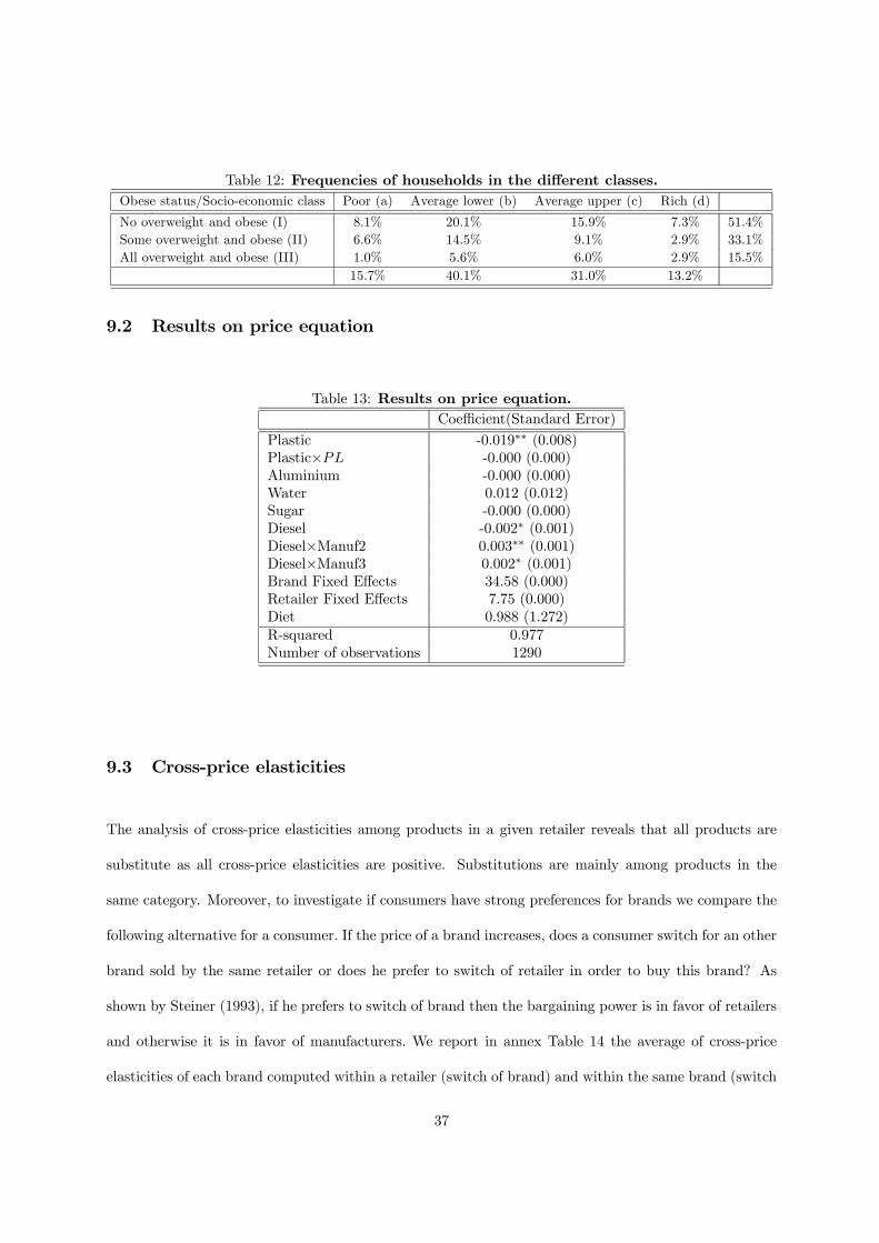
Table 12: Frequencies of households in the different classes.Obese status/Socio-economic class Poor (a) Average lower (b) Average upper (c) Rich (d)

No overweight and obese (I) 8.1% 20.1% 15.9% 7.3% 51.4%Some overweight and obese (II) 6.6% 14.5% 9.1% 2.9% 33.1%All overweight and obese (III) 1.0% 5.6% 6.0% 2.9% 15.5%

15.7% 40.1% 31.0% 13.2%

9.2 Results on price equation

Table 13: Results on price equation.Coefficient(Standard Error)

Plastic -0.019∗∗ (0.008)Plastic×PL -0.000 (0.000)Aluminium -0.000 (0.000)Water 0.012 (0.012)Sugar -0.000 (0.000)Diesel -0.002∗ (0.001)Diesel×Manuf2 0.003∗∗ (0.001)Diesel×Manuf3 0.002∗ (0.001)Brand Fixed Effects 34.58 (0.000)Retailer Fixed Effects 7.75 (0.000)Diet 0.988 (1.272)R-squared 0.977Number of observations 1290

9.3 Cross-price elasticities

The analysis of cross-price elasticities among products in a given retailer reveals that all products are

substitute as all cross-price elasticities are positive. Substitutions are mainly among products in the

same category. Moreover, to investigate if consumers have strong preferences for brands we compare the

following alternative for a consumer. If the price of a brand increases, does a consumer switch for an other

brand sold by the same retailer or does he prefer to switch of retailer in order to buy this brand? As

shown by Steiner (1993), if he prefers to switch of brand then the bargaining power is in favor of retailers

and otherwise it is in favor of manufacturers. We report in annex Table 14 the average of cross-price

elasticities of each brand computed within a retailer (switch of brand) and within the same brand (switch

37

of retailers). Results are mixed. For the leading brand, consumers prefer to switch of retailer in order

to buy their preferred brand rather than switching of brands within a given retailer. However, for other

brands, consumers (slightly) prefer to swith of brand within a given retailer.

Table 14: Cross-price elasticities of brands.

Brands Characteristic Within a retailer Between same brands

B1 R 0.001 (0.001) 0.000 (0.000)B2 D 0.001 (0.001) 0.000 (0.000)B3 R 0.027 (0.022) 0.048 (0.040)B4 D 0.011 (0.009) 0.008 (0.006)B5 R 0.005 (0.004) 0.010 (0.000)B6 D 0.001 (0.001) 0.000 (0.000)B7 R 0.003 (0.003) 0.000 (0.000)B8 R 0.005 (0.004) 0.001 (0.001)B9 D 0.004 (0.003) 0.000 (0.000)B10 R 0.004 (0.003) 0.001 (0.000)B11 R 0.003 (0.002) 0.000 (0.000)B12 R 0.001 (0.001) 0.000 (0.000)B13 R 0.002 (0.002) 0.000 (0.000)B14 R 0.004 (0.003) 0.002 (0.001)B15 R 0.004 (0.003) 0.001 (0.001)B16 R 0.014 (0.011) 0.015 (0.013)B17 D 0.002 (0.002) 0.001 (0.001)

9.4 Price-cost margins

38

Table 15: Margins for the prefered model.Brands Total margins Retailers Total margins

in % in %B1 56.32 (1.20) R1 45.92(0.49)B2 55.22 (1.07) R2 45.07 (1.01)B3 50.04 (0.43) R3 47.29 (0.62)B4 49.74 (0.58) R4 48.23 (0.75)B5 48.18 (0.66) R5 46.85 (0.56)B6 48.28 (0.52) R6 48.37 (1.21)B7 48.45 (0.47)B8 47.40 (0.22)B9 49.38 (0.30)B10 50.43 (1.03)B11 49.33 (0.59)B12 51.35 (1.18)B13 49.30 (0.54)B14 42.14 (1.23)B15 32.95 (1.52)B16 38.08 (0.72)B17 57.01 (1.16)

39