Targeting the Hard-Core Poor: An Impact Assessment

Targeting the Hard-Core Poor: An Impact Assessment

Abhijit Banerjee, Esther Du�o, Raghabendra Chattopadhyay

and Jeremy Shapiro �

This Draft: October, 2010

�We thank Bandhan, in particular Mr. Ghosh and Ramaprasad Mohanto, for their tireless support and collaboration, JyotiPrasad Mukhopadhyay, Abhay Agarwal and Sudha Kant for their research assistance, Prasid Chakraborty for his work collectingdata, CGAP and the Ford Foundation for funding, Biotech International for donating bednets and, especially, Annie Du�o,Lakshmi Krishnan, Justin Oliver and the Center for Micro�nance for their outstanding support of this project.

PRELIMINARY: DO NOT CITE

1

Abstract

It has been noted than many anti-poverty programs, notably micro�nance, fail to reach the poorest

of the poor. This study reports the results of a randomized evaluation of a program designed to

reach this demographic, assist them in establishing a reliable stream of income and "graduate" them to

micro�nance. Our results indicate that this particular intervention, which includes the direct transfer

of productive assets and additional training, succeeds in elevating the economic situation of the poorest.

We �nd that the program results in a 15% increase in household consumption and has positive impacts

on other measures of household wealth and welfare, such as assets and health.


2

1 Introduction

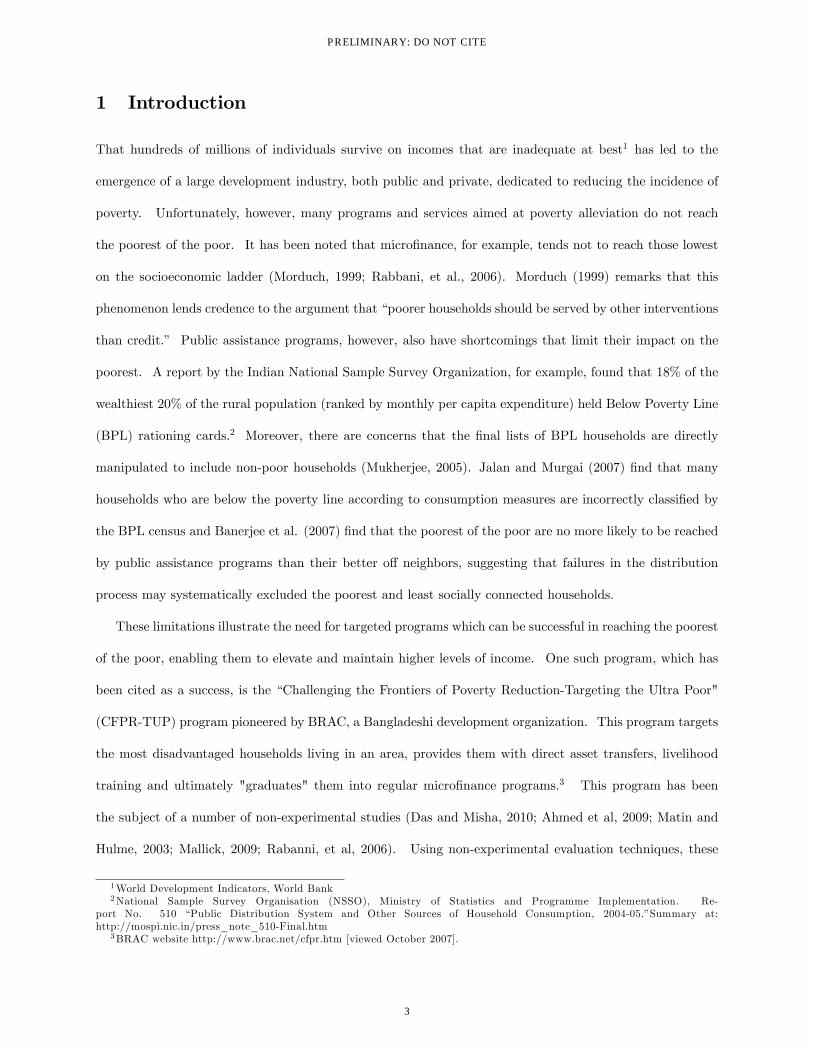
That hundreds of millions of individuals survive on incomes that are inadequate at best1 has led to the

emergence of a large development industry, both public and private, dedicated to reducing the incidence of

poverty. Unfortunately, however, many programs and services aimed at poverty alleviation do not reach

the poorest of the poor. It has been noted that micro�nance, for example, tends not to reach those lowest

on the socioeconomic ladder (Morduch, 1999; Rabbani, et al., 2006). Morduch (1999) remarks that this

phenomenon lends credence to the argument that �poorer households should be served by other interventions

than credit.� Public assistance programs, however, also have shortcomings that limit their impact on the

poorest. A report by the Indian National Sample Survey Organization, for example, found that 18% of the

wealthiest 20% of the rural population (ranked by monthly per capita expenditure) held Below Poverty Line

(BPL) rationing cards.2 Moreover, there are concerns that the �nal lists of BPL households are directly

manipulated to include non-poor households (Mukherjee, 2005). Jalan and Murgai (2007) �nd that many

households who are below the poverty line according to consumption measures are incorrectly classi�ed by

the BPL census and Banerjee et al. (2007) �nd that the poorest of the poor are no more likely to be reached

by public assistance programs than their better o¤ neighbors, suggesting that failures in the distribution

process may systematically excluded the poorest and least socially connected households.

These limitations illustrate the need for targeted programs which can be successful in reaching the poorest

of the poor, enabling them to elevate and maintain higher levels of income. One such program, which has

been cited as a success, is the �Challenging the Frontiers of Poverty Reduction-Targeting the Ultra Poor"

(CFPR-TUP) program pioneered by BRAC, a Bangladeshi development organization. This program targets

the most disadvantaged households living in an area, provides them with direct asset transfers, livelihood

training and ultimately "graduates" them into regular micro�nance programs.3 This program has been

the subject of a number of non-experimental studies (Das and Misha, 2010; Ahmed et al, 2009; Matin and

Hulme, 2003; Mallick, 2009; Rabanni, et al, 2006). Using non-experimental evaluation techniques, these

1World Development Indicators, World Bank2National Sample Survey Organisation (NSSO), Ministry of Statistics and Programme Implementation. Re-

port No. 510 �Public Distribution System and Other Sources of Household Consumption, 2004-05.�Summary at:http://mospi.nic.in/press_note_510-Final.htm

3BRAC website http://www.brac.net/cfpr.htm [viewed October 2007].


3

studies generally �nd very positive program impacts on household�s asset base and consumption.

Based on this apparent success, international donors have taken interest in the program and especially in

rigorously evaluating the e¤ects of programs modeled on BRAC�s CFPR-TUP. CGAP (Consultative Group

to Assist the Poor) and the Ford Foundation have sponsored the implementation and evaluation of 9 similar

programs in 7 countries.4 This paper presents the results from an experimental impact evaluation of this

type of anti-poverty program.

Working with Bandhan, a micro�nance institution based in West Bengal, India, we conducted baseline

and post-program surveys with nearly 1,000 households, half of which were randomly selected to be invited

to participate in Bandhan�s "Targeting the Hard-core Poor" (THP) program. This program is modeled on

BRAC�s CFPR-TUP and incorporates the same elements: asset transfer, livelihood training and graduation

to micro�nance. The program is described in greater detail below.

Using experimentally generated variation in program participation, we �nd that the program results in

substantive improvements in household welfare. Notably, our estimates suggest that the o¤er to participate

in the THP program leads to a 15% increase in per capita monthly consumption. This estimate re�ects the

expected impact of the o¤er to participate and, therefore, takes into account that not all households will

take up the program when o¤ered. Households which actually chose to participate in the THP program

experienced an average increase in per capita monthly consumption of greater than 25%.

Given that the program includes direct asset transfers, mostly livestock, it is not surprising that we also

�nd that treatment households, or those o¤ered the chance to participate in the THP program, have a larger

asset base than comparable control households. We �nd that households derive some income from these

animals, primarily through the sale of livestock. Further results, however, cause us to speculate that the

increase in consumption is due to treatment households leveraging the program to increase income from

small-scale households enterprises (such as bamboo weaving or bidi making).

We �nd a number of additional bene�ts accrue to members of treatment households. In particular,

they su¤er less from food insecurity, they report being happier and are more likely to report that their

physical health has improved. In spite of this latter results, we do not detect program e¤ects in terms of

4Ethiopia, Haiti, Honduras, Pakistan, Peru, Yemen and three locations in India.http://www.cgap.org/p/site/c/template.rc/1.26.12411/


4

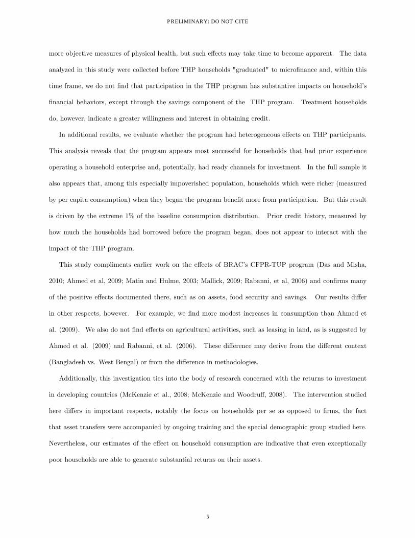
more objective measures of physical health, but such e¤ects may take time to become apparent. The data

analyzed in this study were collected before THP households "graduated" to micro�nance and, within this

time frame, we do not �nd that participation in the THP program has substantive impacts on household�s

�nancial behaviors, except through the savings component of the THP program. Treatment households

do, however, indicate a greater willingness and interest in obtaining credit.

In additional results, we evaluate whether the program had heterogeneous e¤ects on THP participants.

This analysis reveals that the program appears most successful for households that had prior experience

operating a household enterprise and, potentially, had ready channels for investment. In the full sample it

also appears that, among this especially impoverished population, households which were richer (measured

by per capita consumption) when they began the program bene�t more from participation. But this result

is driven by the extreme 1% of the baseline consumption distribution. Prior credit history, measured by

how much the households had borrowed before the program began, does not appear to interact with the

impact of the THP program.

This study compliments earlier work on the e¤ects of BRAC�s CFPR-TUP program (Das and Misha,

2010; Ahmed et al, 2009; Matin and Hulme, 2003; Mallick, 2009; Rabanni, et al, 2006) and con�rms many

of the positive e¤ects documented there, such as on assets, food security and savings. Our results di¤er

in other respects, however. For example, we �nd more modest increases in consumption than Ahmed et

al. (2009). We also do not �nd e¤ects on agricultural activities, such as leasing in land, as is suggested by

Ahmed et al. (2009) and Rabanni, et al. (2006). These di¤erence may derive from the di¤erent context

(Bangladesh vs. West Bengal) or from the di¤erence in methodologies.

Additionally, this investigation ties into the body of research concerned with the returns to investment

in developing countries (McKenzie et al., 2008; McKenzie and Woodru¤, 2008). The intervention studied

here di¤ers in important respects, notably the focus on households per se as opposed to �rms, the fact

that asset transfers were accompanied by ongoing training and the special demographic group studied here.

Nevertheless, our estimates of the e¤ect on household consumption are indicative that even exceptionally

poor households are able to generate substantial returns on their assets.


5

2 Setting and Data

2.1 Overview of Bandan�s �Targeting the Ultra Poor�

In light of evidence that micro�nance does not reach the poorest of the poor (Morduch 1999, Rabbani, et al.

2006) various initiatives have begun which aim to "graduate" the poorest to micro�nance. The intervention

operated by Bandhan is intended to ease credit constraints for exceptionally poor individuals by helping

them establish a reliable income stream. To that end, Consultative Group to Assist the Poor (CGAP)

provided $30,000 as grants for the purchase of income generating assets to be distributed to households

identi�ed as �Ultra Poor.�Grants of $100 were distributed to 300 bene�ciaries residing in rural villages in

Murshidabad, India (a district north of Kolkata) by Bandhan. The design of this program was based on

the pioneering work of BRAC, a Bangladeshi development organization. For several years, BRAC has been

distributing grants through its �Challenging the Frontiers of Poverty Reduction-Targeting the Ultra Poor"

(CFPR-TUP) program with the aim of helping the absolute poorest graduate to micro�nance.5 Working in

close consultation with BRAC, Bandhan developed the criteria to identify the Ultra Poor.

The initial phase of the intervention consists of Bandhan identifying those eligible for the grants; the

poorest of the poor within each village. To classify such household Bandhan used a set of criteria adapted

from those used by BRAC in their CFPR-TUP program. Firstly, an eligible household must have an able-

bodied female member. The rationale for this requirement is that the program is intended particularly

to bene�t women6 and any bene�t accruing from the grant requires that the bene�ciary be capable of

undertaking some enterprise. The second mandatory requirement is that the household not be associated

with any micro�nance institution (in keeping with the aim of targeting those who lack credit access) or

receive su¢ cient support through a government aid program.7 In addition to these two criteria, eligible

households should meet three of the following �ve criteria: the primary source of income should be informal

labor or begging, land holdings below 20 decimals (10 katthas, 0.2 acres), no ownership of productive assets

5BRAC website http://www.brac.net/cfpr.htm [viewed October 2007].6While the majority of bene�ciaries are female, some men were identi�ed as eligible under special circumstances such as

physical disability.7�Su¢ cient support�was determined on a case-by-case basis by Bandhan; while many of the households they identi�ed as

Ultra Poor participate in some government aid program, they determined that this assistance was not su¢ cient to alleviate thepoverty of the household.


6

other than land, no able bodied male in the household and having school-aged children working rather than

attending school.

To identify those households satisfying this de�nition of Ultra Poor, Bandhan utilized a multi-phase

process. The initial task is to identify the poorer hamlets in the region. Since Bandhan has operations

in Murshidabad, this is accomplished by consulting with local branch managers who are familiar with the

economic conditions in these villages.

In the second phase, Bandhan conducts Participatory Rural Appraisals (PRAs) in particular hamlets of

selected villages to identify the subset of the population most likely to be Ultra Poor. To ensure that the

PRA includes a su¢ cient number of participants, Bandhan employees enter the hamlet on the day prior

to the PRA; they meet with teachers and other local �gures to build rapport with the residents, announce

that the PRA will occur on the following day and encourage participation. Bandhan aims for 12-15 PRA

participants, but often the �gure is as high as 20. Moreover, they encourage household members from various

religions, castes and social groups to attend.

The PRA consists of social mapping and wealth ranking. In the �rst stage the main road and any

prominent hamlet landmarks (temples, mosques, rivers, etc.) are etched into the ground, usually in front

of a central house in the hamlet. Subsequently the participants enumerate each household residing in the

hamlet and mark the location of the households on the hamlet map. For each household, the name of the

household head is recorded on an index card.

In the wealth ranking stage, the index cards are sorted into piles corresponding to socioeconomic status.

To accomplish this, Bandhan�s employees select one of the index cards and inquire about that household�s

occupation, assets, land holdings and general economic well-being. They then take another card and ask

how this household compares to the prior household. A third card is selected, classi�ed as similar in wealth

to one or the other of the prior households and then whether it is better o¤ or worse o¤ than that household.

This process is continued until all the cards have been sorted into piles, usually 5 of them, corresponding to

poverty status (the �fth pile representing the poorest group). Often a large percentage of the cards end up

in the �fth pile, in which case these households are sorted in a similar manner into two or more piles.

Following the PRA, Bandhan selects the households assigned to the lowest few ranks, progressively taking


7

higher categories until they have approximately 30 households. In the second phase of their identi�cation

process a Bandhan employee visits these households to conduct a short questionnaire. The questionnaire

pertains to the criteria for Ultra Poor classi�cation; inquiring about the presence of an able-bodied woman,

the presence and ability to work of a male household head, land holdings, assets, NGO membership and so

on. Based on the information collected in this survey, Bandhan narrows its list of potentially Ultra Poor

households in that hamlet to 10-15.

In the �nal stage of the process, the project coordinator, who is primarily responsible for administration of

this program, visits the households. He veri�es the questionnaire through visual inspection and conversations

with the household members. Final identi�cation as Ultra Poor is determined by the project coordinator,

according to the established criteria and his subjective evaluation of the households�economic situation.

Following identi�cation, half of the potential bene�ciaries were randomly selected to receive assets. Rather

than transferring cash, Bandhan procures assets, such as livestock or inventory, and distributes them to

bene�ciaries. The grants are also used to �nance other inputs, such as fodder and sheds to house the

animals. Following selection, Bandhan sta¤met with bene�ciaries to select the livelihood option best suited

to the household. In this sample bene�ciaries predominantly chose livestock, receiving either 2 cows, 4 goats

or 1 cow and 2 goats; of the bene�ciaries surveyed in the endline 240 had selected livestock while 33 had

taken non-farm enterprises.

Over the following 18 months, Bandhan sta¤met weekly with bene�ciaries. These meetings accomplished

multiple objectives. Firstly, Bandhan utilized these meetings to provide information and training on a

number of topics related to the households enterprise (such as proper care for livestock) as well as regarding

broader social and health issues.8 Additionally, bene�ciaries were required to save Rs. 10 (approximately

$US 0.25) per week at these meetings and, �nally, Bandhan disbursed a weekly "subsistence allowance" of

Rs. 90 at these meetings. The duration of the subsistence allowance depended on the particular enterprise

selected by the households and ranged from 13 to 40 weeks.9

Approximately eighteen months after receipt of the asset, the bene�ciaries were "graduated" to micro�-

8These topics included: Early Marriage, HIV/ AIDS, S anitation & Personal health, Immunisation, Fruits tree plantation,Women & child tra¢ cking, Family planning, Dowry, De-worming and Marriage Registration.

9The exact duration was 13 weeks for households which selected a non-farm enterprise, 30 weeks for households receivinggoats and 40 weeks for households receiving cows.


8

nance and became eligible for regular micro�nance loans provided by Bandhan. As most of the ultra poor

households did not have prior experience with a formal �nancial institution, such as a bank or MFI, Bandhan

conducted a three day long micro credit orientation training course for the THP program bene�ciaries, which

was mandatory to be considered eligible for loan disbursement. The training addressed a number of social,

health and community issues10 as well as explaining the functioning of a micro credit group, its rules and

regulations, group solidarity and the role of savings in one�s �nancial life. The endline survey discussed

below, and utilized in the analysis, was generally conducted before the graduation training. At the time

of writing, however, the majority of bene�ciaries had joined one of Bandhan�s micro�nance groups and had

taken a loan.

2.2 Data

The data used in this study comprise two waves of surveying. The initial wave, spanning from February

2007 to March 2008, was conducted among those households identi�ed as Ultra Poor by Bandhan. The

survey consists of a household module, covering income, consumption, migration and various other features

of the household. It also included an adult module, which was administered to all adults (over 18 years old)

in the household, inquiring, among other topics, about labor supply, time use, health and aspirations.

Following the completion of the baseline survey, households were randomly selected to receive an o¤er

to participate in the program. Randomization was done remotely by the research team, and selection was

strati�ed on hamlet (a sub unit within village). A total of 991 baseline surveys were conducted, of which

512 (51.66%) were randomly selected for program participation.11 The �gure of 512 exceeds the number

of households which actually received assets as a non-negligible fraction of households were either found to

be ineligible between randomization and enterprise selection (on account of participating in micro�nance

activities or self-help groups) or refused the o¤er to participate. Of the 512 o¤ers to participate, 26612

10These topics included generating awareness of the role of village committees (formed by Bandhan), dincouraging dowry andearly marriage, raising awareness about basic human rights and the role of the government and local self governments (such asthe Panchayat, and Gram Sabha) and fostering awareness about health, safe drinking water and sanitation.11A total of 13 households were not randomized. The names of 11 households were inadvertently left of the list of names for

randomization and 2 households were directly selected by Bandhan to receive assets later in the course of the study. We omitthese households from the analysis.12262 originally accepted, 4 of those randomly selected to participate later received an asset from another household (e.g.

returned assets) retransfered by Bandhan.


9

individuals participated in the program, 64 were found ineligible before asset transfer13 and 156 declined to

participate. 26 individuals initially participated in the program, but decided later not to and returned the

asset.14

Of the 991 households administered the baseline, 11 were inadvertently left o¤ a list of names to be

randomized. Two other households received assets from households which had returned the assets later

on. We surveyed these households later, but they were not chosen randomly; rather Bandhan selected these

households. We omit these 13 households from the analysis.

Of the 978 households included in the study, 818 (84%) were found again in the endline which was

conducted 18 months after asset transfer, although 6 chose not to take the survey. In addition we conducted

an endline interview with 2 households who were part of the list of households for randomization, but who

refused the baseline survey.15 Our �nal sample consists of these 814 households of which 428 were randomly

selected to participate in the program and 25716 held assets from Bandhan at the time of the endline survey.

3 Empirical Strategy

In the results that follow, we estimate the causal impact the THP program on a number of household and

individual level outcomes, including income, consumption, health, food security and labor supply, which are

denoted by y. Letting Si be an indicator variable that household i was randomly selected to participate in

the THP program, we estimate the following equation

yih = �Sih + �h + "ih (1)

where the subscript h indicates hamlet (a sub-unit of villages). We include hamlet level �xed e¤ects

1316 had a micro�nance loan, 29 were members of SHGs and others were found ineligible for various reasons (migrated beforbeing contacted, too old to care for asset, receiving other government assistance, etc.).14This ocurred for a variety of reasons; when the household migranted Bandhan often retransfered the asset to another

household. This also happened if the bene�ciary died or became unable to care for the asset. Also some households electedto return the asset; anecdotally, this was due to misperceptions that the program was associated with a Christian organizationseeking converts. Apparantly, a similar occurrence happened with BRAC�s parallel program in Bangladesh (see Mallick, 2009).15Although randomization was customarily done after the completion of the baseline, 3 households were mistakenly included

on the list for randomization before the baseline was complete. We revisited these households after discovering but theydeclined to give the interview at that point. 2 of these households were found for the endline.16251 of these were selected to receive the assets randomly. The remaining 6 were selected by Bandhan to receive assets later

on (usuall they received an asset that was returned by another household).


10

given that randomization was strati�ed at the hamlet level. Random o¤ers of program participation ensure

that Sih is not correlated with "ih and that we recover the true causal impact of the program on the outcome.

This is measured by � which captures the mean di¤erence in y between those who were o¤ered program

participation and those that were not after removing the e¤ect of common hamlet level determinates of y.

� does not measure the actual impact of participating in the program on the outcome of interest, but

rather the expected change in the outcome for a household which is o¤ered the chance to participate.

We report these Intent to Treat (ITT) estimates (as opposed to the Treatment on the Treated, or TOT,

estimates) given that these estimates give the expected impact and are most relevant to the issue of scaling

up the program.17

Additionally, where baseline data is available, we estimate a di¤erence-in-di¤erence speci�cation given

by

yiht = �1Sih + �2E + �3Sih � E + �h + "ih (2)

where E is an indicator variable for the data deriving from the endline survey and t indexes time (0 for

baseline and 1 for endline). As these results are generally very similar to those from equation (1) we note

di¤erences below but omit the results (they are available from the authors on request).

For individual level outcomes we estimate

yijh = �Sih + �h + "ih + "ijh (3)

where the subscript j denotes individual j residing in household i. When reporting results for individual

level outcomes we cluster standard errors at the household level, re�ecting the likely possibility of correlation

within households.

17The TOT results can be estimated by scaling the ITT results by a factor of 1 divided by the di¤erence in participation(having an asset) between treatment and control groups, which is 1

251428

� 6385

= 1:75:


11

4 Results

4.1 Attrition

While the empirical strategy outlined above provides internally consistent estimates of the program impact,

the results may lack external validity and su¤er from bias if there is unbalanced attrition; meaning that the

probability that we were able to reach the household for a follow up survey is correlated with some other factor

which in�uences the outcomes of interest. To understand how the sample which we were able to resurvey

di¤ers from the entire study population, we compare the means of various household characteristics, as

measured in the baseline survey, between households which we surveyed in the endline and those that we

did not.

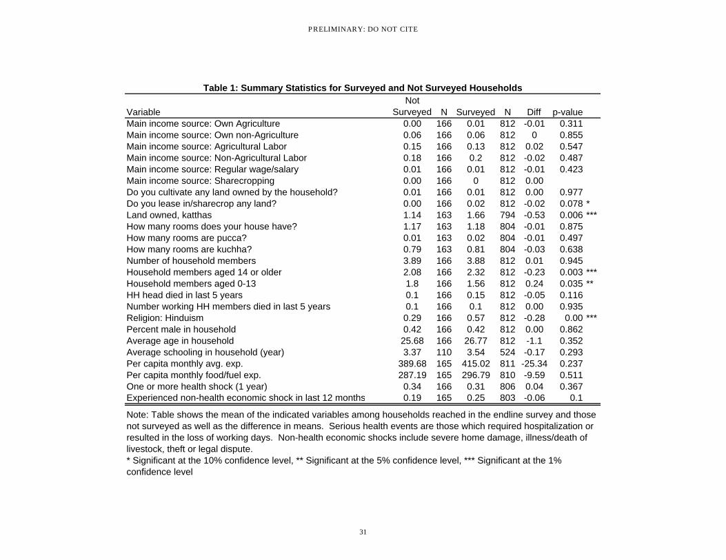
Table 1 shows that households which we were not able to resurvey di¤er along various dimensions: they

have less land, tend to have fewer adult household members (and more children; the average total number of

members is the same for both groups) and are more likely to be Muslim. These di¤erences accord with the

reasons for failure to resurvey recorded by enumerators. Land and household composition, for example, may

be correlated with migration; households which were not resurveyed were more likely to migrate, but the

di¤erence is not statistically signi�cant. That rumors that Bandhan was a Christian organization seeking

converts circulated in some Muslim communities explains the greater reluctance of Muslims to participate

in the endline survey, and thus the di¤erence in religious a¢ liation between the groups.

These di¤erences alone, however, do not necessarily entail bias. Only if attrition is unbalanced across

the treatment and control groups should we be concerned about bias. To assess this concern, we regress

an indicator variable that the household was an attrition household (surveyed at baseline but not endline)

on an indicator that the household was selected to participate in the program (Sih). Table 2 shows that

treatment assignment is not a signi�cant predictor of attrition, which mitigates concerns about attrition bias

a¤ecting the results.


12

4.2 Summary Statistics

Another assumption underlying the empirical strategy is that the randomization was in fact successful and

baseline characteristics are uncorrelated with treatment assignment. We assess this assumption in Panel A

of Table 3, which shows the means, and di¤erence in means, of baseline characteristics for treatment and

control households. Of the 25 variables considered we only detect a signi�cant di¤erence between treatment

and control households with respect to a single outcome: the percentage of households reporting regular

wages as a primary household income source (a very small fraction of control households, 2%, report such

income while no treatment households do). These estimates indicate that the randomization was successful.

Panel B reveals substantive di¤erences between treatment and control households at the endline, indicat-

ing e¤ects of the program. In particular households randomly selected for participation in the program are

signi�cantly more likely to report that their main source of household income derives from non-agricultural

enterprises operated by the household and less likely to report it comes from agricultural labor. They are

also 12% more likely to cultivate some of their land, signi�cant at the 1% con�dence level. There are also

highly signi�cant di¤erences (above a 1% con�dence level) between treatment and control in terms of per

capita consumption, with treatment households consuming approximately 15% more per person per month.

Finally, it appears that treatment households are more likely to report experiencing a non-health related

economic shock in the last year; as death of livestock is included in the variable as constituting a shock, this

may also be an outcome of the program. In what follows we investigate these and other outcomes in greater

detail.

4.3 Assets and Income

Before examining potential e¤ects on household consumption and well-being, we explore how program partic-

ipation changes the composition of household income and a¤ects asset formation. In Figure 1, we illustrate

the distribution of primary income sources reported by households, separately for the baseline and endline

survey and broken out by treatment status. The �gure shows that there are no evident di¤erences between

treatment and control households at baseline, but at endline it appears that treatment households are more

likely to report that their main source of income derives from non-agricultural self-employment or wages and


13

less likely to report relying on agricultural labor.

In Figure 2, we present a similar illustration pertaining to whether any household members engage in

the indicated activity. This �gure shows that, in the endline, treatment households are much more likely

to engage in livestock and farming activities. A notable contrast between this �gure and Figure 1 is that

while a roughly similar percentage of control households report receiving income from a non-agricultural

enterprise, the di¤erence between the fraction of treatment and control households reporting this in their

primary income source is more pronounced.

The increase in the percentage of households engaging in animal rearing activities is not surprising given

that livestock was the primary enterprise selected by bene�ciaries. In Table 4, we document the increase in

livestock holdings brought about by the THP program. The table shows that households o¤ered a chance

to participate in the program have acquired, on average, approximately 2 more animals over the past 3

years; 1.5 small animals (goats, pigs or sheep) and 0.4 cows. The table also indicates that this livestock

has generated income for the household; primarily from irregular income sources, de�ned as the sale of the

animal itself, animal products (such as skin or hide) or animal calves. Considering monthly �ow income

from animals, which captures income from milk, eggs and other animal products less regular expenses such

as fodder, we �nd that, on average, the cost of maintaining livestock exceeds regular �ow income from these

animals, and that this is especially true for treatment households, who tend to own more animals. This

does not imply that rearing livestock is, on balance, not pro�table (since income from items such as the sale

of calves is captured elsewhere) but that maintaining livestock represents a monthly cost, or investment, and

that treatment households incur this cost to a larger extent than control households.

In columns 7-10 we consider assets more broadly. Column 7 takes the quantity of land owned by the

household as the dependent variable; we �nd that treatment households own about 13 of a katta more land

than control households, signi�cant at the 10% con�dence level. Column 8 shows that treatment households

have, on average, 0.5 additional fruit trees, the planting of which was actively encouraged by Bandhan.

Finally, we aggregate asset holdings into an index using principal component analysis. Our index includes

ownership of livestock as well as of productive assets and durable household items.18 Column 9 indicates

18The list of speci�c items includes: TV Set, Radio / Transistor / Stereo, Electric Fan, Refrigerator, Telephone / Mobilephone, Bicycle, Rickshaw/Van, Sewing machines, Chair / stool, Cot, Table, Watch / Clock, Pairs of shoes/sandals and Golas


14

that treatment households score higher on this index, a di¤erence which is statistically signi�cant above a 1%

con�dence level. The di¤erence is also economically meaningful, representing 25% of the standard deviation

of the index. To check whether the increase in assets derives solely from the assets directly transferred by

Bandhan, or if the program also fosters asset creation beyond the transfer, we replicate the analysis from

column 9 in column 10 using an index that excludes ownership of livestock. The point estimate suggests

that treatment households own more household assets and durable goods, but the estimate is not statistically

signi�cant.

Since Figure 2 indicates there may be a di¤erent propensity for treatment and control households to

engage in agricultural production and non-agricultural enterprises, we test for treatment e¤ects along these

dimensions. Tables 5 and 6 present these results. We do not �nd any statistically signi�cant di¤erence

between treatment and control households in terms of land cultivated (either owned or leased), or their

propensity to �sh or income from �shing. Nor can we detect any di¤erence in the probability that the

household operates a non-agricultural enterprise or income from such an enterprise in the last 30 days.

4.4 Consumption

We �nd that the program alters the composition of household income, and appears to augment income

deriving from several sources. Income, however, is notoriously di¢ cult to measure and, therefore, we

consider the e¤ect of the program on household consumption; both as a measure of the economic impact of

the THP program and because consumption is a crucial metric of welfare.

Figures 5-7 graphically depict the e¤ect of the THP program on per capita consumption. The �gures

plot the density of per capita monthly consumption (separately for total consumption, for food and fuel

consumption and for non-food consumption) for treatment and control households. For total consumption

as well as food and fuel consumption, the density for treatment households is more or less uniformly shifted

rightward, indicating that the program increased consumption at all levels of consumption. For non-

food consumption the distributions are quite similar, except that the distribution for treatment households

includes a longer right tail, indicating the presence of a few exceptionally high expenditure levels on non-food

/ talas (structures for storing grains).


15

items among treatment households.

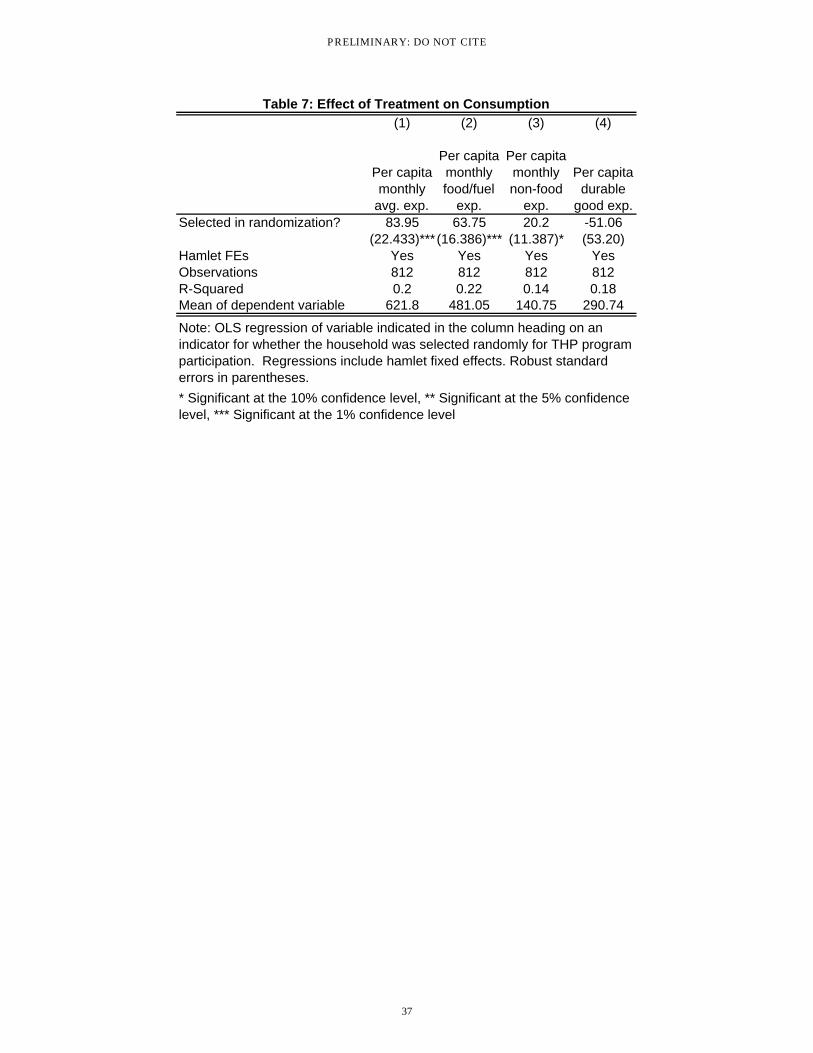
We check whether these di¤erences are statistically signi�cant in Table 7, which presents results from

estimating equation (1) when taking these measures of consumption as the dependent variable. The point

estimates imply that treatment households spend, on average, Rs. 84 per person per month in total than

control households, and Rs. 64 more on food and fuel. These di¤erences are statistically di¤erent from zero

above a 1% con�dence level. The estimates imply that treatment households spend Rs. 20 more per person

per month on non-food items, signi�cant at the 10% level. But Figure 7 suggests this is driven by a few

outliers. Finally, in column 4, we investigate whether treatment households are acquiring more household

durables, but can not reject that the expenditure levels between treatment and control are equal in this

respect.

We should note that in addition to being highly statistically signi�cant, the results with respect to total

and food consumption are also of considerable magnitude; these di¤erences represent approximately 15% of

the mean level of consumption among the control group.

In Table 8, we disaggregate the gains in food consumption across food groups. We �nd that the increase

was more or less uniform across all food groups. But in percentage terms the largest increases were in fruits

& nuts, dairy and meat & eggs, suggesting that program participants were consuming more nutritious food

than members of control households.

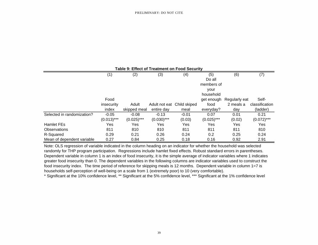
The increase in the quantity and nutritional value of food consumed by treatment households would

be expected to impact their perceptions and reports of food security, which is what we �nd in Table 9.

Column 1 of the table takes an index of food insecurity as the dependent variable. The results indicate that,

predictably, treatment households score lower on this index. The di¤erence is statistically signi�cant above

the 1% con�dence level. Columns 2-6 consider di¤erences in individual components of the food insecurity

index. The results suggest that the di¤erence in food insecurity is primarily driven by adults in treatment

households eating more and more regularly than comparable adults in control households. The �nal column

reports the di¤erence in the households self-perception of their current �nancial situation on a scale from 1

(worst) to 10 (best). Treatment households report a score which is 0.2 points, or 7%, higher than control

households.


16

For these consumption outcomes (total consumption, food consumption and food item consumption) the

diference-in-di¤erence estimates, available on request, are slightly higher but generally consistent with the

results discussed above.

4.5 Financial Behaviors and Con�dence

The ultimate aim of the program is to enable individuals to establish a regular income stream and "graduate"

them into micro�nance groups. Since our data was gathered before Bandhan conducted training sessions

and integrated THP bene�ciaries into their micro�nance activities, we are not able to evaluate this process

(a second follow up survey is ongoing). Nevertheless, we investigate whether treatment households exhibit

di¤erent attitudes and behaviors with respect to saving and borrowing than control households, which may

be indicative of the ease with which bene�ciaries will transition into micro�nance.

Columns 1-3 of Table 10 indicate that 18 months after entering the program, bene�ciary households do

not have greater credit access than non-bene�ciary households; in total or considering informal credit (e.g.

moneylenders or shopkeepers) or quasi-formal credit (e.g. micro�nance) separately. Treatment households,

however, appear to save more than control households; depositing an average of Rs. 56 in the last 30 days

into their accounts compared to the Rs. 34 deposited by control households (although this di¤erence is not

statistically signi�cant in the di¤erence-in-di¤erence speci�cation).

Mostly this savings occurs through the accounts held by Bandhan, thus we can not conclusively say

whether this is additional savings, or a shift in savings held at home into the account with Bandhan.

Although we do not detect any di¤erence in actual credit, our survey included several hypothetical

questions about ones willingness to borrow. Households were asked whether they would be interested in

borrowing Rs. 1,000, 2,000, 5,000 or 8,000 at 12.5% interest (�at). Respondents in treatment households

indicate that they would be willing to borrow 17% more than respondents in control households.

Finally, bene�ciaries (women in the household who actually received the asset) score higher on an index of

�nancial autonomy than potential bene�ciaries (women identi�ed as eligible residing in control households).

The index is constructed from variables indicating that the (potential) bene�ciary participates in �nancial

decisions made in the household. The di¤erence in the index is driven entirely by the fact that women in


17

treatment households are more likely to be personally responsible for savings accounts, which were part of

the program provided by Bandhan.

4.6 Sharing and Crowd-out

Given that this intervention took place in rural villages, where bene�ciary households know and are known

by other households, we investigate whether receiving assistance through the THP program crowds out

assistance provided by the community. In Table 11 we regress the number of meals given or received by the

household and the value of food, gifts and loans given or received by the household on an indicator that the

household was randomly selected to participate in the THP program and hamlet �xed e¤ects.

We �nd that selected households have given an additional 0.7 meals in the last 30 days to other households,

signi�cant above a 5% con�dence level, and report receiving Rs. 17 less (over 50% less) in gifts of food from

other households in the last month than control households. We do not observe statistically signi�cant

results for other outcomes, but the point estimates are generally consistent with the notion that selected

households receive less in gifts and loans from other community members than control households.

In unreported results (available on request) we evaluate whether participation in the THP crowds out

government assistance administered by local government o¢ cials (such as subsidized food). We do not

�nd that selection for participation in the THP program results in any di¤erential probability of receiving

government assistance.

4.7 Individual Level Impacts

In addition to surveying a knowledgeable member of the household about that household�s situation, we also

administered an individuals survey to each adult member of the household (18 years or more), allowing us

to investigate the impact of the THP program on individual outcomes such as time use and health.

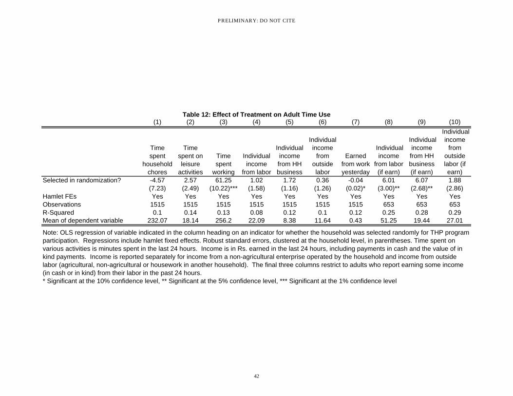
Table 12 shows how adults in treatment and control households report spending their time. It evaluates

di¤erences between members of treatment and control households in terms of the average quantity of time

allocated to work, leisure and household chores. The table suggests that adults in treatment households

increased the quantity of time spent working by an additional hour a day (signi�cant at the 1% con�dence


18

level). We also consider earnings from this work in columns 4-9. Considering all adults, we do not �nd

that adults in treatment households report earning more in the last 24 hours from their labor than adults in

control households. The majority of adults, however, do not report earning anything from their activities in

the last 24 hours. We �nd that adults in treatment households are slightly less likely to report having earned

money from their activities the previous day (column 7); this di¤erence is signi�cant at the 10% level, but not

especially large compared to the average propensity to report income (43%). Among those adults who do

report earning income from their activities, members of treatment households earn, on average, Rs. 6 more

than members of control households. The di¤erence is signi�cant at the 5% con�dence level. It appears that

this additional earning derives from enterprises operated by the household; members of treatment households

earn Rs.6 more from operating household enterprises than members of control households. This di¤erence is

signi�cant at the 5% con�dence level and represents nearly 30% of the mean daily earnings from household

enterprises.

Table 13 investigates time allocation in more depth, revealing that the additional hour per day spent

working by adults in treatment households is entirely accounted for by increased time spent tending livestock.

This �nding, coupled with our failure to detect any signi�cant di¤erence between treatment and control

households with respect to their propensity to operate a non-farm enterprise suggests that the program may

have augmented income from small household enterprises by facilitating investment rather than the creation

of new enterprises.

We examine the allocation of children�s time in Table 14, which does not suggest any clear di¤erences in

how children residing in treatment and control households spend their time. This table reports results from

estimating equation (3) when taking child�s time use on various activities as the dependent variable. Since

we asked each adult member about the time their children spend on various activities, we often obtained

multiple reports for the same child (one from each parent). Panel A of Table 14 uses only data reported by

(potential) bene�ciaries on how her children spend their time. The point estimates indicate that children

of women o¤ered the opportunity to participate in the program study 30-40 additional minutes a day when

compared to children of other potential bene�ciaries, signi�cant at the 10% level. There are no statistically

signi�cant di¤erences with respect to other categories of time use however, and the di¤erence with respect


19

to time studying is not statistically di¤erent from zero when averaging both parent�s reports of how their

children spend their time and considering children of non-bene�ciaries residing in the household (Panel B).

Finally, Table 15 shows result pertaining to health outcomes. We �nd that adults residing in treatment

households score higher on an index of health knowledge and behaviors which is constructed using principal

components analysis of questions pertaining to health behaviors and knowledge, such as hand washing,

having soap in the household and knowledge of diseases and disease prevention techniques. We do not

�nd any e¤ects on actual health outcomes, such as lost working days to illness or Activities of Daily Living

(ADL) scores. We do, however, �nd that adults residing in treatment households are 6% more likely to

perceive that their health has improved over the last year (signi�cant at the 1% con�dence level). We also

�nd that these adults are less likely to report symptoms of mental distress and have a more positive outlook

on the future, as measured by an index of mental health on which individuals from treatment households

score higher.

Given that the program also incorporated an education campaign around social and health issues, we

evaluate di¤erences in knowledge and attitudes about social issues. In Table 16 we �nd that members of

treatment households think that families should have fewer children, are more likely to indicate that there

is legal punishment for taking dowry and are more likely to self-report vaccinating children. We do not �nd

any signi�cant di¤erences in knowledge about legal ages for marriage or voting.

Finally, in Table 17, we evaluate whether the program in�uences political involvement and women�s

empowerment. Given that the program was targeted at women, and engaged them economically, it is

possible that this would in�uence their degree of autonomy and, potentially, engagement in local politics.

We do not �nd that there are any di¤erences between treatment and control households in terms of political

involvement. We do �nd that women in treatment households score higher on our index of autonomy

than women in control households. The di¤erence is driven entirely by women in treatment households

having their own �nancial resources, separate from the resources of the household, which is likely the savings

accounts held with Bandhan; we do not �nd substantial di¤erences along other dimensions, such as women�s

freedom to travel.


20

5 Heterogeneity

The goal of the THP program is to reach the poorest of the poor, assist them in establishing a regular income

stream, enable them to partake in microcredit services and prevent them from falling back into extreme

poverty. It is crucial to the success of this program that the very poorest are able to use this program to

build assets, start businesses and obtain greater access to credit. In what follows, we assess whether there

are heterogeneous program impacts for some of the main e¤ects. We focus on household consumption, as

it is perhaps our best measure of the overall economic impact of the program and an important welfare

metric, the existence of and income from household enterprises, as this appears to be a source from which

treatment households derive income, and �nancial behaviors, as increasing credit access is a main goal of the

program. We consider heterogeneous e¤ects along several dimensions: baseline consumption, as a general

measure of poverty, prior borrowing history, indicative of ability to obtain credit, and the prior existence

of a household enterprise, as an indicator of entrepreneurship and experience. To estimate heterogeneous

e¤ects we estimate

yih = �1Sih + �2Xih + �3Xih � Sih + �h + "ih (4)

where y is one of the outcomes discussed above and X is either baseline per capita monthly total con-

sumption, the rupee value of debt taken by the household in the 12 months before the baseline or an indicator

variable for the household operating a small non-farm enterprise at the time of the baseline survey.

The results with respect to endline consumption are show in Table 18. The top panel shows that there

are di¤erential program impacts based on initial household consumption. The point estimate implies that

each additional rupee of baseline consumption leads to a 0.27 rupee additional impact of the program on

endline consumption. The interaction e¤ect is statistically signi�cant at the 10% con�dence level. This

point estimate suggests that going from the 25th to the 75th percentile of baseline consumption (a di¤erence

of Rs. 217) leads to an expected program impact 57 rupees higher, approximately 24 of the average program

e¤ect. This appears largely driven by the tail of the distribution however, given that we �nd positive

treatment e¤ects on consumption at all levels of consumption in the analysis above.

We do not observe any heterogeneous e¤ects based on credit history, but �nd that households which


21

had a non-farm enterprise at baseline experience a treatment e¤ect on per capita total consumption of

approximately Rs. 150 larger than treatment households which did not have an enterprise initially. In this

speci�cation the main treatment e¤ect enters at the 1% con�dence level and the interaction term enters at

the 5% con�dence level. When considering per capita food and fuel consumption, the coe¢ cient on the

interaction term is only marginally signi�cant. These results, however, appear driven by the upper tail of the

distribution; when we omit the top 1% of the sample, ranked by baseline per capita monthly consumption,

the interaction term in no longer enters the regression at conventional signi�cance levels.

Turning to heterogeneous e¤ects on credit (total credit and credit from informal and quasi-formal sources)

at endline, in Table 19, we do not �nd that either prior consumption, prior credit history or the prior existence

of a household enterprise result in heterogeneous program impacts on household credit access at endline.

In Table 20, we do �nd some indication of heterogeneous e¤ects on the pro�ts of household enterprises.

We fail to �nd such e¤ects with respect to the existence of or investment in household enterprises, but

it appears that households which were richer at the time of the baseline and households which operated

an enterprise at the baseline bene�t to a larger extent from the THP program in terms of growing their

enterprise. The estimates imply that each additional rupee of baseline consumption leads to an expected

program impact on household enterprise pro�ts 0.32 rupees higher; or that a treatment household at the

75th percentile of baseline consumption would be expected to have enterprise pro�ts Rs. 65 higher than a

treatment household at the 25th percentile of baseline consumption. This coe¢ cient on the interaction term

enters at the 10% con�dence level. But again, when we omit the highest 1% of the baseline consumption

distribution, the coe¢ cient on the interaction term is not statistically distinguishable from zero. We do �nd,

however, that a treatment household which had a preexisting household enterprise is expected to earn pro�ts

from household enterprises which are Rs. 323 higher than the expected pro�ts from a treatment household

without a pre-existing enterprise. In this case the coe¢ cient is signi�cant at the 5% con�dence level.

6 Conclusion

In this study we report the results of a randomized impact assessment of an anti-poverty program targeted

at the poorest of the poor in rural villages of West Bengal, India. The program, operated by a local


22

micro�nance institution, makes direct asset transfers to women residing in poor households, to enable them

to establish a reliable income source and "graduate" them into regular micro�nance groups.

We �nd that this program was successful in notable respects. In particular we �nd that participation

in the program results in substantial increases in per capita household consumption. This e¤ect appears

especially large for households which operated a pre-existing small-scale household enterprise. We also �nd

various other bene�ts, such as reduced food insecurity, increased assets and some indication of improved

health. Although the data analyzed in this study was collected before bene�ciaries joined micro�nance

groups, we �nd that program participants express greater interest in obtaining credit, although we do not

detect any e¤ect on current �nancial behaviors.

This particular intervention is modeled on BRAC�s pioneering CFPR-TUP program, which also targets

the "ultra poor" with asset transfers and graduates them to micro�nance, and has been replicated in various

countries around the globe. The results from this experimental impact evaluation suggest that this type of

intervention represents a viable strategy to reach the poorest of the poor and enable them to move up the

economic ladder.


23

References

Akhter U. Ahmed, Mehnaz Rabbani, Munshi Sulaiman, and Narayan C. Das. The impact of asset transfer

on livelihoods of the Ultra Poor in Bangladesh. Research Monograph Series, Research and Evaluation

Division, BRAC, Dhaka., No. 39, 2009.

Sajeda Amin, Ashok S. Rai, and Giorgio Topa. Does microcredit reach the poor and vulnerable? Evidence

from northern Bangladesh. Journal of Development Economics, 70(1):59�82, February 2003.

Abhijit Banerjee, Esther Du�o, Raghabendra Chattopadhyay, and Jeremy Shapiro. Targeting e¢ ciency:

How well can we identify the poor? Center for Micro�nance Working Paper, 2007.

Narayan C Das and Farzana A Misha. Addressing extreme poverty in a sustainable manner: Evidence

from CFPR programme. CFPR Working Paper No. 19, 2010.

Angus Deaton. The Analysis of Household Surveys. The Johns Hopkins University Press, Baltimore, 1997.

Jyotsna Jalan and Rinku Murgai. An e¤ective "Targeting Shortcut"? An assessment of the

2002 below-poverty line census method. http://www.ihdindia.org/ourcontrol/rinku_murgai.doc,

2007. Viewed September 2007.

Debdulal Mallick. How e¤ective is a big push for the small? Evidence from a quasi-random experiment.

mimeo, 2009.

Imran Matin and David Hulme. Programs for the poorest: Learning from the igvgd program in bangladesh.

World Development, 31(3):647 �665, 2003.

Jonathan Morduch. The micro�nance promise. Journal of Economic Literature, 37(4):1569�1614, 1999.

Neela Mukherjee. Political corruption in India�s Below the Poverty Line (bpl) exercise: Grassroots�

perspectives on BPL: Good practice in people�s participation from Bhalki village, West Bengal.mimeo,

2005.

Mehnaz Rabbani, Vivek Prakash, and Munshi Sulaiman. Impact assessment of CFPR/TUP: A descriptive

analysis based on 2002-2005 panel data. CFPR/TUP Working Paper Series, No. 12, 2006.

Patrick Webb, Jennifer Coates, and Robert Houser. Does microcredit meet the needs of all poor women?


24

Constraints to participation among destitute women in Bangladesh. Tufts University Food Policy and

Applied Nutrition Program Discussion Paper, No. 3, 2002.

Christopher Woodru¤ and David McKenzie. Experimental evidence on returns to capital and access to

�nance in Mexico. World Bank Economic Review, 22(3):457�482, 2008.

Christopher Woodru¤, David McKenzie, and Suresh de Mel. Returns to capital: Results from a randomized

experiment. Quarterly Journal of Economics, 123(4):1329�1372, 2008.


25

Figure 1


26

Figure 2


27

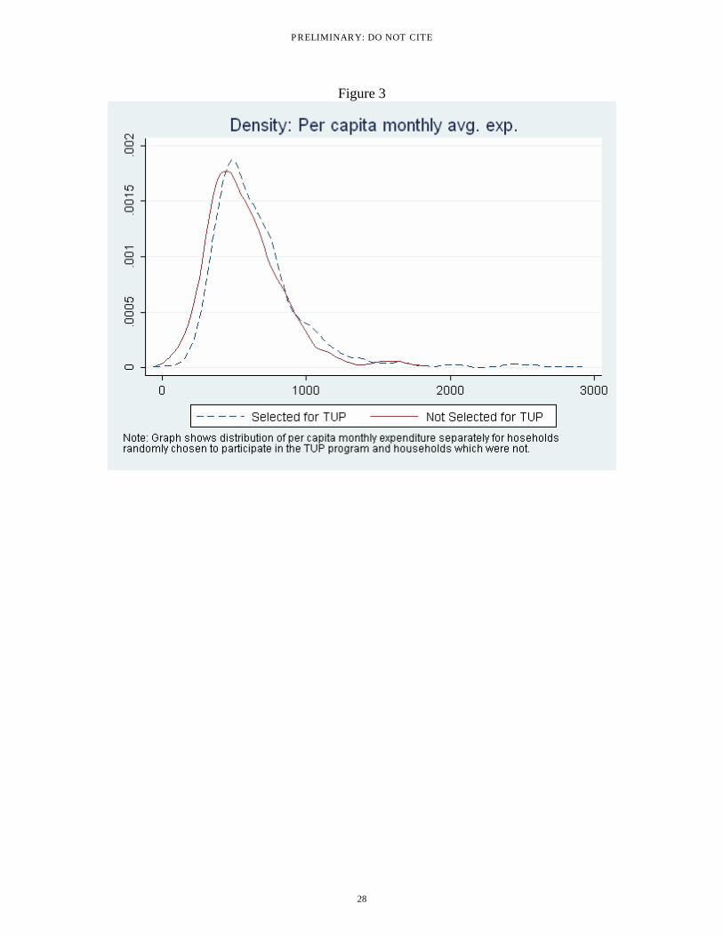
Figure 3


28

Figure 4


29

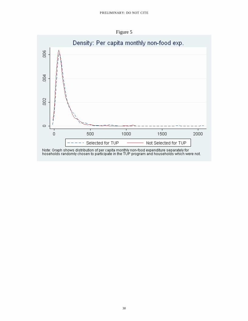
Figure 5


30

VariableNot

Surveyed N Surveyed N Diff p-value Main income source: Own Agriculture 0.00 166 0.01 812 -0.01 0.311 Main income source: Own non-Agriculture 0.06 166 0.06 812 0 0.855 Main income source: Agricultural Labor 0.15 166 0.13 812 0.02 0.547 Main income source: Non-Agricultural Labor 0.18 166 0.2 812 -0.02 0.487 Main income source: Regular wage/salary 0.01 166 0.01 812 -0.01 0.423 Main income source: Sharecropping 0.00 166 0 812 0.00 Do you cultivate any land owned by the household? 0.01 166 0.01 812 0.00 0.977 Do you lease in/sharecrop any land? 0.00 166 0.02 812 -0.02 0.078 *Land owned, katthas 1.14 163 1.66 794 -0.53 0.006 ***How many rooms does your house have? 1.17 163 1.18 804 -0.01 0.875 How many rooms are pucca? 0.01 163 0.02 804 -0.01 0.497 How many rooms are kuchha? 0.79 163 0.81 804 -0.03 0.638 Number of household members 3.89 166 3.88 812 0.01 0.945 Household members aged 14 or older 2.08 166 2.32 812 -0.23 0.003 ***Household members aged 0-13 1.8 166 1.56 812 0.24 0.035 **HH head died in last 5 years 0.1 166 0.15 812 -0.05 0.116 Number working HH members died in last 5 years 0.1 166 0.1 812 0.00 0.935 Religion: Hinduism 0.29 166 0.57 812 -0.28 0.00 ***Percent male in household 0.42 166 0.42 812 0.00 0.862 Average age in household 25.68 166 26.77 812 -1.1 0.352 Average schooling in household (year) 3.37 110 3.54 524 -0.17 0.293 Per capita monthly avg. exp. 389.68 165 415.02 811 -25.34 0.237 Per capita monthly food/fuel exp. 287.19 165 296.79 810 -9.59 0.511 One or more health shock (1 year) 0.34 166 0.31 806 0.04 0.367 Experienced non-health economic shock in last 12 months 0.19 165 0.25 803 -0.06 0.1

Table 1: Summary Statistics for Surveyed and Not Surveyed Households

Note: Table shows the mean of the indicated variables among households reached in the endline survey and those not surveyed as well as the difference in means. Serious health events are those which required hospitalization or resulted in the loss of working days. Non-health economic shocks include severe home damage, illness/death of livestock, theft or legal dispute.* Significant at the 10% confidence level, ** Significant at the 5% confidence level, *** Significant at the 1% confidence level


31

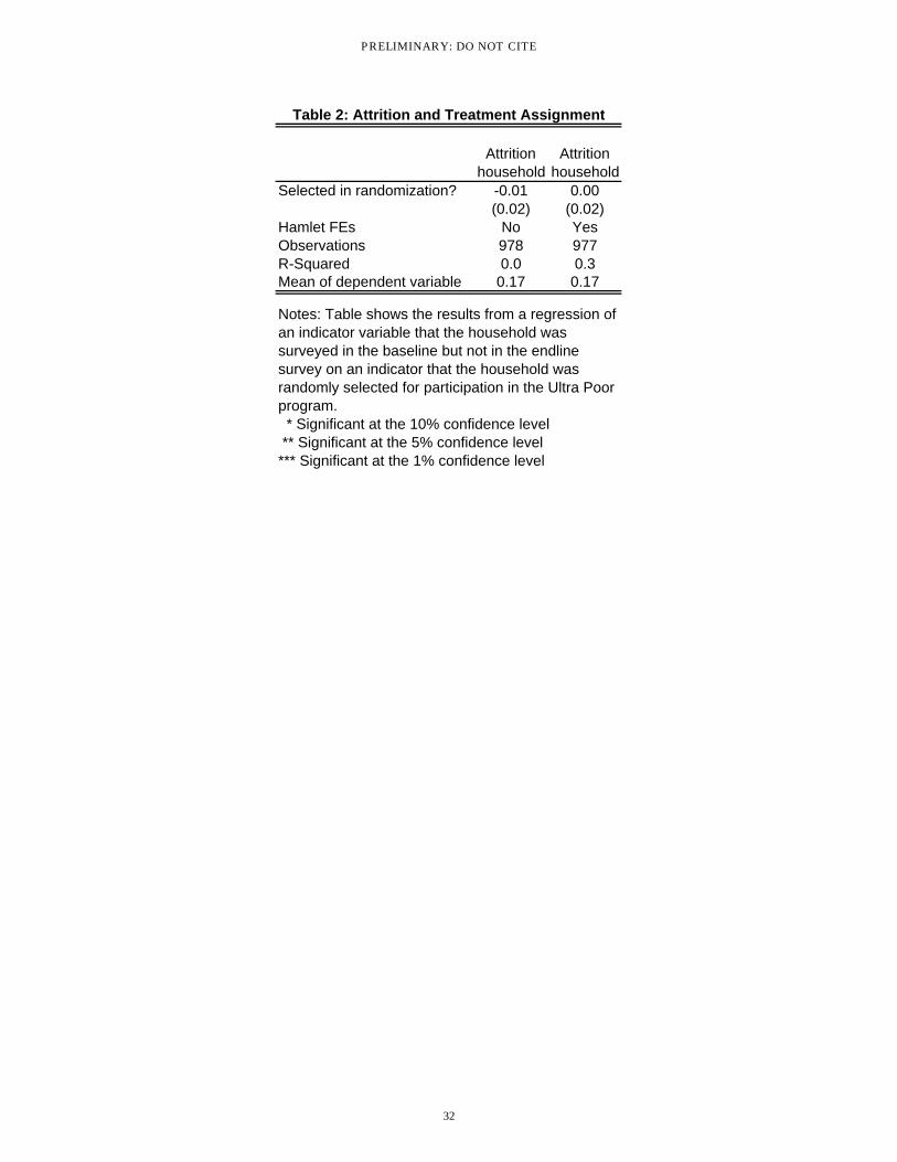
Attrition

householdAttrition

householdSelected in randomization? -0.01 0.00 (0.02) (0.02)Hamlet FEs No YesObservations 978 977R-Squared 0.0 0.3Mean of dependent variable 0.17 0.17

*** Significant at the 1% confidence level

Table 2: Attrition and Treatment Assignment

Notes: Table shows the results from a regression of an indicator variable that the household was surveyed in the baseline but not in the endline survey on an indicator that the household was randomly selected for participation in the Ultra Poor program. * Significant at the 10% confidence level ** Significant at the 5% confidence level


32

Variable Selected NNot

Selected N Diff p-value Main income source: Own Agriculture 0.00 427 0.01 385 0.00 0.572 Main income source: Own non-Agriculture 0.07 427 0.05 385 0.02 0.295 Main income source: Agricultural Labor 0.12 427 0.15 385 -0.03 0.231 Main income source: Non-Agricultural Labor 0.19 427 0.22 385 -0.03 0.357 Main income source: Regular wage/salary 0.00 427 0.02 385 -0.02 0.021 **Main income source: Sharecropping 0.00 427 0.00 385 0.00 Do you cultivate any land owned by the household? 0.01 427 0.01 385 0.00 0.869 Do you lease in/sharecrop any land? 0.02 427 0.02 385 0.00 0.953 Land owned, katthas 1.63 418 1.69 376 -0.06 0.718 How many rooms does your house have? 1.18 422 1.17 382 0.01 0.651 How many rooms are pucca? 0.03 422 0.02 382 0.01 0.727 How many rooms are kuchha? 0.79 422 0.84 382 -0.05 0.266 Number of household members 3.91 427 3.84 385 0.07 0.52 Household members aged 14 or older 2.36 427 2.26 385 0.10 0.137 Household members aged 0-13 1.55 427 1.57 385 -0.02 0.818 HH head died in last 5 years 0.16 427 0.14 385 0.02 0.506 Number working HH members died in last 5 years 0.10 427 0.09 385 0.01 0.658 Religion: Hinduism 0.58 427 0.56 385 0.03 0.433Percent male in household 0.43 427 0.4 385 0.03 0.114Average age in household 26.8 427 26.74 385 0.06 0.952Average schooling in household (year) 3.56 275 3.52 249 0.04 0.782Per capita monthly avg. exp. 411.41 427 419.04 384 -7.63 0.676Per capita monthly food/fuel exp. 295.07 427 298.7 383 -3.63 0.772One or more health shock (1 year) 0.29 424 0.33 382 -0.05 0.149Experienced non-health economic shock in last 12 months 0.24 420 0.26 383 -0.03 0.406

Variable Selected NNot

Selected N Diff p-value Main income source: Own Agriculture 0.01 428 0.01 386 0.01 0.202 Main income source: Own non-Agriculture 0.32 428 0.24 386 0.08 0.01 ***Main income source: Agricultural Labor 0.19 428 0.26 386 -0.07 0.021 **Main income source: Non-Agricultural Labor 0.32 428 0.27 386 0.05 0.157 Main income source: Regular wage/salary 0.00 428 0.01 386 -0.01 0.344 Main income source: Sharecropping 0.00 428 0.00 386 0.00 0.179 Do you cultivate any land owned by the household? 0.66 428 0.55 384 0.12 0.001 ***Do you lease in/sharecrop any land? 0.06 428 0.04 383 0.02 0.262 Land owned, katthas 1.47 422 1.21 383 0.26 0.105 How many rooms does your house have? 1.26 428 1.26 385 0.00 0.957 How many rooms are pucca? 0.02 428 0.02 385 0.00 0.862 How many rooms are kuchha? 0.72 428 0.75 385 -0.03 0.584 Number of household members 3.95 428 4.21 386 -0.26 0.437 Household members aged 14 or older 2.48 428 2.41 385 0.07 0.307 Household members aged 0-13 1.49 423 1.49 379 0.00 0.965 Able bodied male adult (18+) 0.69 428 0.67 386 0.02 0.525 HH head died in last 5 years 0.11 428 0.10 386 0.01 0.696 Number working HH members died in last 5 years 0.12 428 0.07 386 0.04 0.04 **Religion: Hinduism 0.61 428 0.57 385 0.04 0.30 Percent male in household 0.43 428 0.42 386 0.01 0.68 Average age in household 28.49 428 28.54 385 -0.05 0.956 Average schooling in household (year) 3.65 298 3.6 263 0.05 0.732 Per capita monthly avg. exp. 663.28 428 575.75 385 87.53 0.00 ***Per capita monthly food/fuel exp. 514.3 428 444.07 385 70.22 0.00 ***One or more health shock (1 year) 0.42 426 0.41 385 0.01 0.883 Experienced non-health economic shock in last 12 months 0.38 428 0.21 386 0.17 0.00 ***

* Significant at the 10% confidence level, ** Significant at the 5% confidence level, *** Significant at the 1% confidence level

Table 3: Summary StatisticsPanel A

Panel B

Note: Table shows the mean of the indicated variables among households randomly selected to receive an offer to participate in the THP program and those that were not as well as the difference in means. Panel A presents results from the baseline survey and Panel B presents results from the endline survey. Serious health events are those which required hospitalization or resulted in the loss of working days. Non-health economic shocks include severe home damage, illness/death of livestock, theft or legal dispute.


33

(1) (2) (3) (4) (5) (6) (7) (8) (9) (10)

Small animals acquired (3 years)

Goats, pigs or sheep

acquired (3 years)

Birds acquired (3 years)

Cows acquired (3 years)

Irregular income

from livestock

Monthly flow

income from

livestock

Land owned, katthas

Number fruit trees

Assets index

(durables and

livestock)

Assets index

(durables)Selected in randomization? 1.95 1.52 0.42 0.4 398.83 -82.05 0.28 0.56 0.39 0.12 (0.191)*** (0.119)*** (0.136)*** (0.053)*** (78.960)***(23.662)*** (0.169)* (0.249)** (0.119)*** (0.12)Hamlet FEs Yes Yes Yes Yes Yes Yes Yes Yes Yes YesObservations 811 811 811 802 811 810 804 809 796 797R-Squared 0.28 0.35 0.2 0.34 0.24 0.16 0.14 0.16 0.2 0.18Mean of dependent variable 1.91 1.11 0.79 0.33 256.28 -73.38 1.34 1.66 0.38 0.32

Table 4: Effect of Treatment on Livestock and Assets

Note: OLS regression of variable indicated in the column heading on an indicator for whether the household was selected randomly for THP program participation. Regressions include hamlet fixed effects. Robust standard errors in parentheses. Irregular income includes income derived from the sale of animals, sale of animal calves or sale of products (hides, etc.) of deceased animals over the prior 3 years. Monthly flow income includes income from home consumption or sale of milk, dung (for fuel), wool, or other animal products. Assets index is the principal components index of household durable goods and livestock owned by the household or durables alone (as indicated in the column heading).* Significant at the 10% confidence level, ** Significant at the 5% confidence level, *** Significant at the 1% confidence level


34

(1) (2) (3) (4)

Own land cultivated (katthas)

Leased land cultivated (katthas)

Household fishes

Income from fishing

(30 days)Selected in randomization? -0.03 0.15 -0.01 -101.95 (0.17) (0.36) (0.02) (116.10)Hamlet FEs Yes Yes Yes YesObservations 811 810 812 811R-Squared 0.07 0.22 0.37 0.17Mean of dependent variable 0.23 1.05 0.09 200.47

Note: OLS regression of variable indicated in the column heading on an indicator for whether the household was selected randomly for THP program participation. Regressions include hamlet fixed effects. Robust standard errors in parentheses. Land cultivated refers to the sum of land area cultivated in each season.

Table 5: Effect of Treatment on Income from Agriculture and Fishing



35

(1) (2) (3)

Operate small

enterprise

Investment in small

enterprise

Enterprise income (1

month)Selected in randomization? 0.03 -1.58 41.51 (0.03) (37.09) (40.91)Hamlet FEs Yes Yes YesObservations 813 804 797R-Squared 0.36 0.26 0.27Mean of dependent variable 0.51 201.87 319.25

Table 6: Effect of Treatment on Income from Non-farm Enterprises

Note: OLS regression of variable indicated in the column heading on an indicator for whether the household was selected randomly for THP program participation. Regressions include hamlet fixed effects. Robust standard errors in parentheses. Variables refer to any enterprise operated within the last 3 years. Investment refers to investment in any non-merchandise item necessary to operate the enterprise. Income is net of expenses.* Significant at the 10% confidence level, ** Significant at the 5% confidence level, *** Significant at the 1% confidence level


36

(1) (2) (3) (4)

Per capita monthly

avg. exp.

Per capita monthly food/fuel

exp.

Per capita monthly non-food

exp.

Per capita durable

good exp.Selected in randomization? 83.95 63.75 20.2 -51.06 (22.433)***(16.386)*** (11.387)* (53.20)Hamlet FEs Yes Yes Yes YesObservations 812 812 812 812R-Squared 0.2 0.22 0.14 0.18Mean of dependent variable 621.8 481.05 140.75 290.74

Table 7: Effect of Treatment on Consumption

Note: OLS regression of variable indicated in the column heading on an indicator for whether the household was selected randomly for THP program participation. Regressions include hamlet fixed effects. Robust standard errors in parentheses.* Significant at the 10% confidence level, ** Significant at the 5% confidence level, *** Significant at the 1% confidence level


37

(1) (2) (3) (4) (5) (6) (7) (8) (9) (10)

Exp.

cerealsExp.

pulses Exp. dairyExp.

edible oilExp.

vegetablesExp. fruit,

nuts

Exp. meat, eggs

Exp. other food

Exp. pan, tobac., alcohol

Exp. fuel and light

Selected in randomization? 15.02 2.61 4.74 2.82 15.14 3.01 8.26 8.76 0.47 2.91 (5.340)*** (1.387)* (1.678)*** (1.667)* (4.276)*** (1.142)*** (2.548)*** (2.686)*** (2.28) (2.96)Hamlet FEs Yes Yes Yes Yes Yes Yes Yes Yes Yes YesObservations 812 812 812 812 812 812 812 812 812 812R-Squared 0.2 0.22 0.22 0.21 0.22 0.23 0.22 0.22 0.15 0.23Mean of dependent variable 167.64 15.49 12.51 38.24 98.06 7.37 30.08 54.62 19.5 37.54Effect as % of mean 9% 17% 38% 7% 15% 41% 27% 16% 2% 8%

Table 8: Effect of Treatment on Disaggregated Food Consumption

Note: OLS regression of variable indicated in the column heading on an indicator for whether the household was selected randomly for THP program participation. Regressions include hamlet fixed effects. Robust standard errors in parentheses. All variables are per capita.* Significant at the 10% confidence level, ** Significant at the 5% confidence level, *** Significant at the 1% confidence level


38

(1) (2) (3) (4) (5) (6) (7)

Food insecurity

indexAdult

skipped mealAdult not eat

entire dayChild skiped

meal

Do all members of

your household get enough

food everyday?

Regularly eat 2 meals a

day

Self-classification

(ladder)Selected in randomization? -0.05 -0.08 -0.13 -0.01 0.07 0.01 0.21 (0.013)*** (0.025)*** (0.030)*** (0.03) (0.025)*** (0.02) (0.072)***Hamlet FEs Yes Yes Yes Yes Yes Yes YesObservations 811 810 810 811 811 811 810R-Squared 0.29 0.21 0.26 0.24 0.2 0.25 0.24Mean of dependent variable 0.27 0.84 0.25 0.18 0.16 0.92 2.91

Table 9: Effect of Treatment on Food Security

Note: OLS regression of variable indicated in the column heading on an indicator for whether the household was selected randomly for THP program participation. Regressions include hamlet fixed effects. Robust standard errors in parentheses. Dependent variable in column 1 is an index of food insecurity, it is the simple average of indicator variables where 1 indicates greater food insecurity than 0. The dependent variables in the following columns are indicator variables used to construct the food insecurity index. The time period of reference for skipping meals is 12 months. Dependent variable in column 1=7 is households self-perception of well-being on a scale from 1 (extremely poor) to 10 (very comfortable).* Significant at the 10% confidence level, ** Significant at the 5% confidence level, *** Significant at the 1% confidence level


39

(1) (2) (3) (4) (5) (6) (7) (8) (9)

Total

borrowingInformal

borrowingQuasi-formal

borrowing

Rs. deposited in savings (30

days)

Willingness to borrow

(min of loan size bounds)

Financial autonomy

index

Decide: buy and sell assets

Decide: spend,

borrow and save.

Responsible for savings accounts.

Selected in randomization? -204.58 -61.83 -142.75 22.62 439.63 0.14 0.03 0 0.38 (371.16) (345.46) (98.85) (10.820)** (216.052)** (0.025)*** (0.04) (0.04) (0.032)***Hamlet FEs Yes Yes Yes Yes Yes Yes Yes Yes YesObservations 811 811 811 804 793 813 793 791 812R-Squared 0.18 0.18 0.18 0.2 0.22 0.21 0.21 0.23 0.34Mean of dependent variable 3206.95 2984.13 222.83 33.99 2519.55 0.39 0.37 0.38 0.42

Table 10: Effect of Treatment on Financial Variables

Note: OLS regression of variable indicated in the column heading on an indicator for whether the household was selected randomly for THP program participation. Regressions include hamlet fixed effects. Robust standard errors in parentheses. The willingness to borrow and financial autonomy variables are constructed only from survey responses of the THP beneficiary or potential beneficiary (for control households). The former pertains to expressed willingness to borrow different amounts of money with interest. The later is the simple average of indicators of financial autonomy (presented separately in the following three columns): specifically taking independent decisions about buying and selling assets, taking decisions about borrowing, spending and saving and operating savings accounts).



40

(1) (2) (3) (4) (5) (6) (7) (8)

Meals

received Meals givenValue food received

Value food given

Loans given to other

households

Gifts given to other

households

Loans received

from other households

Gifts received

from other households

Selected in randomization? 0.99 0.71 -17.59 0.29 -6.76 6.57 -286.76 -138.07 (0.87) (0.327)** (9.392)* (0.73) (14.74) (11.79) (291.37) (382.92)Hamlet FEs Yes Yes Yes Yes Yes Yes Yes YesObservations 807 811 788 811 797 797 797 797R-Squared 0.19 0.18 0.14 0.07 0.12 0.13 0.2 0.14Mean of dependent variable 6.1 1.78 30.11 1.02 23.51 17.97 1575.97 991.27

Table 11: Effect of Treatment on Transfers

Note: OLS regression of variable indicated in the column heading on an indicator for whether the household was selected randomly for THP program participation. Regressions include hamlet fixed effects, which correspond roughly to villages. Robust standard errors in parentheses. Time period of reference for dependent variables in columns 1-4 is 30 days, in columns 5-8 it is 18 months.* Significant at the 10% confidence level, ** Significant at the 5% confidence level, *** Significant at the 1% confidence level


41

(1) (2) (3) (4) (5) (6) (7) (8) (9) (10)

Time spent

household chores

Time spent on leisure

activities

Time spent

working

Individual income

from labor

Individual income from HH business

Individual income

from outside labor

Earned from work yesterday

Individual income

from labor (if earn)

Individual income from HH business (if earn)

Individual income

from outside labor (if earn)

Selected in randomization? -4.57 2.57 61.25 1.02 1.72 0.36 -0.04 6.01 6.07 1.88 (7.23) (2.49) (10.22)*** (1.58) (1.16) (1.26) (0.02)* (3.00)** (2.68)** (2.86)Hamlet FEs Yes Yes Yes Yes Yes Yes Yes Yes Yes YesObservations 1515 1515 1515 1515 1515 1515 1515 653 653 653R-Squared 0.1 0.14 0.13 0.08 0.12 0.1 0.12 0.25 0.28 0.29Mean of dependent variable 232.07 18.14 256.2 22.09 8.38 11.64 0.43 51.25 19.44 27.01

Note: OLS regression of variable indicated in the column heading on an indicator for whether the household was selected randomly for THP program participation. Regressions include hamlet fixed effects. Robust standard errors, clustered at the household level, in parentheses. Time spent on various activities is minutes spent in the last 24 hours. Income is in Rs. earned in the last 24 hours, including payments in cash and the value of in kind payments. Income is reported separately for income from a non-agricultural enterprise operated by the household and income from outside labor (agricultural, non-agricultural or housework in another household). The final three columns restrict to adults who report earning some income (in cash or in kind) from their labor in the past 24 hours.* Significant at the 10% confidence level, ** Significant at the 5% confidence level, *** Significant at the 1% confidence level

Table 12: Effect of Treatment on Adult Time Use


42

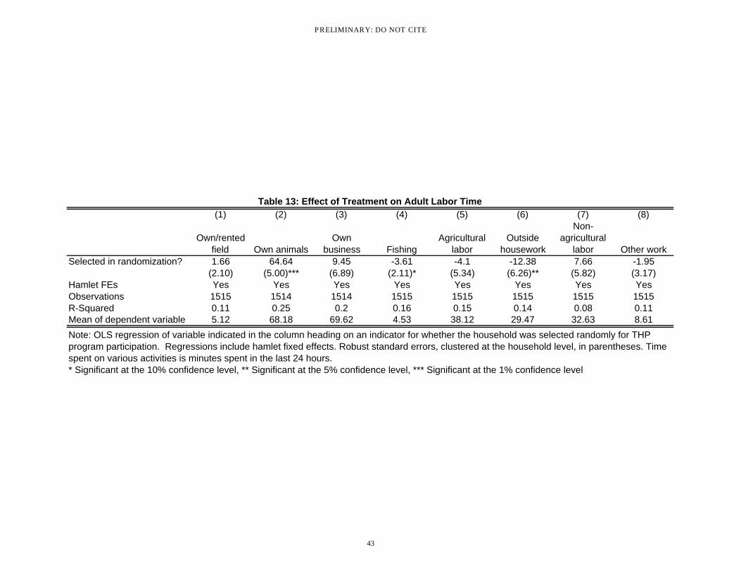
(1) (2) (3) (4) (5) (6) (7) (8)

Own/rented

field Own animalsOwn

business FishingAgricultural

laborOutside

housework

Non-agricultural

labor Other workSelected in randomization? 1.66 64.64 9.45 -3.61 -4.1 -12.38 7.66 -1.95 (2.10) (5.00)*** (6.89) (2.11)* (5.34) (6.26)** (5.82) (3.17)Hamlet FEs Yes Yes Yes Yes Yes Yes Yes YesObservations 1515 1514 1514 1515 1515 1515 1515 1515R-Squared 0.11 0.25 0.2 0.16 0.15 0.14 0.08 0.11Mean of dependent variable 5.12 68.18 69.62 4.53 38.12 29.47 32.63 8.61

Table 13: Effect of Treatment on Adult Labor Time

Note: OLS regression of variable indicated in the column heading on an indicator for whether the household was selected randomly for THP program participation. Regressions include hamlet fixed effects. Robust standard errors, clustered at the household level, in parentheses. Time spent on various activities is minutes spent in the last 24 hours.* Significant at the 10% confidence level, ** Significant at the 5% confidence level, *** Significant at the 1% confidence level


43

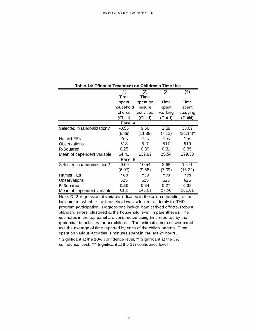
(1) (2) (3) (4)

Time spent

household chores (Child)

Time spent on leisure

activities (Child)

Time spent

working (Child)

Time spent

studying (Child)

Selected in randomization? -0.55 9.66 2.59 38.09 (8.89) (11.39) (7.12) (21.14)*Hamlet FEs Yes Yes Yes YesObservations 518 517 517 519R-Squared 0.25 0.39 0.31 0.35Mean of dependent variable 64.41 139.99 25.54 179.33

Selected in randomization? -0.69 10.54 2.68 19.71 (6.97) (9.68) (7.09) (16.29)Hamlet FEs Yes Yes Yes YesObservations 625 625 625 625R-Squared 0.26 0.34 0.27 0.33Mean of dependent variable 61.8 140.81 27.56 181.01


Panel B

Panel A

Table 14: Effect of Treatment on Children's Time Use

Note: OLS regression of variable indicated in the column heading on an indicator for whether the household was selected randomly for THP program participation. Regressions include hamlet fixed effects. Robust standard errors, clustered at the household level, in parentheses. The estimates in the top panel are constructed using time reported by the (potential) beneficiary for her children. The estimates in the lower panel use the average of time reported by each of the child's parents. Time spent on various activities is minutes spent in the last 24 hours.


44

(1) (2) (3) (4) (5) (6) (7) (8) (9) (10) (11) (12)

Health Knowledge

and Behavior Index Health Index

Unable to work

because sick or injured (30

days)Days unable

to work

Average ADL score (1-

4=can't do task)

Self perception of

health (10=best 1=worst)

Perceive health

improved last year

Mental Health Index

Life satisfaction index (1-5=most

satisfied)

Index of reported

symptoms of mental distress

Did not experience period of

worry/anxiety in last year

Scale (1-3) think life will

get betterSelected in randomization? 0.44 0.11 -0.03 -0.03 -0.02 0.08 0.06 0.41 0.14 -0.08 0.04 0 (0.09)*** (0.07) (0.02) (0.22) (0.02) (0.08) (0.02)*** (0.11)*** (0.04)*** (0.02)*** (0.02)*** (0.01)Hamlet FEs Yes Yes Yes Yes Yes Yes Yes Yes Yes Yes Yes YesObservations 1511 1514 1515 1515 1515 1514 1515 1498 1512 1512 1510 1501R-Squared 0.16 0.16 0.17 0.13 0.14 0.16 0.14 0.19 0.17 0.2 0.14 0.22Mean of dependent variable 0 0 0.36 2.23 1.53 3.97 0.27 0 2.51 0.56 0.09 2.94


Note: OLS regression of variable indicated in the column heading on an indicator for whether the household was selected randomly for THP program participation. Regressions include hamlet fixed effects. Robust standard errors, clustered at the household level, in parentheses. The index of health knowledge and behaviors is constructed using principal components analysis using questions pertaining to health behaviors and knowledge including washing hands after defecating, wearing sandals to the latrine and elsewhere, awareness of waterborne diseases and ways to prevent them, knowledge of HIV and ways to prevent the disease, having soap, a toothbrush and paste at home and knowledge of iodized salt. The index of physical health in a principal component index of various indicators of health, including: self-perception, missed work days, and Activities of Daily Living measures. The index of mental health is also constructed using principal component analysis based on the self-reported presence or lack of symptoms of poor mental health and an individual's outlook for the future.

Table 15: Effect of Treatment on Adult Health


45

(1) (2) (3) (4) (5) (6) (7) (8)

Good # of children to

have

What is the legal age of

marriage for a boy?

What is the legal age of

marriage for a girl?

What is the lowest age for casting vote?

Punishment for giving and taking dowry at marriage?

Mother should be involved in

fertility decision

Do you get your child

administered to vaccines?

Are you aware of the different Government schemes?

Selected in randomization? -0.05 -0.02 0.03 0.07 0.05 0 0.05 -0.01 (0.03)* -0.17 -0.1 -0.16 (0.03)* -0.01 (0.03)* -0.02Hamlet FEs Yes Yes Yes Yes Yes Yes Yes YesObservations 1504 1466 1469 1263 1470 1477 748 1513R-Squared 0.11 0.1 0.11 0.11 0.13 0.14 0.26 0.16Mean of dependent variable 2.14 22.5 18.58 19.19 0.67 0.93 0.88 0.82

Note: OLS regression of variable indicated in the column heading on an indicator for whether the household was selected randomly for THP program participation. Regressions include hamlet fixed effects. Robust standard errors, clustered at the household level, in parentheses. Variation in sample size driven by * Significant at the 10% confidence level, ** Significant at the 5% confidence level, *** Significant at the 1% confidence level

Table 16: Effect of Treatment on Knowledge


46

(1) (2) (3) (4) (5) (6) (7)

Index of political

involvement

Index of women's

autonomy (all)

Index of (potential)

beneficiaries's autonomy

Woman travels out of

village (30 days)

Travels unescorted to next village

Participates in SHG

Has own financial assets

Selected in randomization? 0.01 0.07 0.08 -0.01 -0.02 -0.02 0.35 -0.02 (0.01)*** (0.02)*** -0.03 (0.01)* -0.02 (0.03)***Hamlet FEs Yes Yes Yes Yes Yes Yes YesObservations 1515 1512 758 1490 1511 1511 1512R-Squared 0.12 0.19 0.21 0.16 0.11 0.17 0.28Mean of dependent variable 0.45 0.52 0.53 0.59 0.96 0.14 0.41

Table 17: Effect of Treatment on Empowerment

Note: OLS regression of variable indicated in the column heading on an indicator for whether the household was selected randomly for THP program participation. Regressions include hamlet fixed effects. Robust standard errors, clustered at the household level, in parentheses. Women's autonomy index is the simple average of indicators that the woman can travel outside the village, participation in Self Help Groups or having her own savings and loans; the components are also evaluated separately. This index is also considered exclusively for beneficiaries and potential beneficiaries (in the control group). The index of political involvement is the simple average of indicators that the individual voted in local elections or approached local political officials.* Significant at the 10% confidence level, ** Significant at the 5% confidence level, *** Significant at the 1% confidence level


47

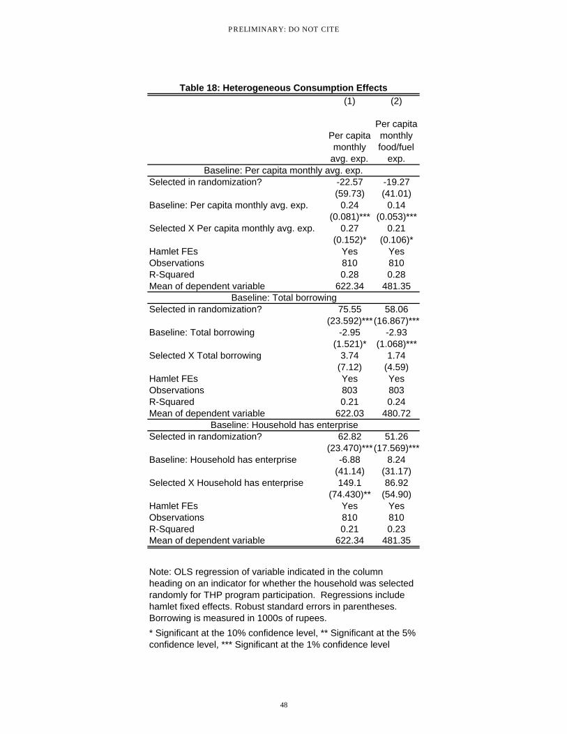
(1) (2)

Per capita monthly

avg. exp.

Per capita monthly food/fuel

exp.

Selected in randomization? -22.57 -19.27 (59.73) (41.01)Baseline: Per capita monthly avg. exp. 0.24 0.14 (0.081)*** (0.053)***Selected X Per capita monthly avg. exp. 0.27 0.21 (0.152)* (0.106)*Hamlet FEs Yes YesObservations 810 810R-Squared 0.28 0.28Mean of dependent variable 622.34 481.35

Selected in randomization? 75.55 58.06 (23.592)***(16.867)***Baseline: Total borrowing -2.95 -2.93 (1.521)* (1.068)***Selected X Total borrowing 3.74 1.74 (7.12) (4.59)Hamlet FEs Yes YesObservations 803 803R-Squared 0.21 0.24Mean of dependent variable 622.03 480.72

Selected in randomization? 62.82 51.26 (23.470)***(17.569)***Baseline: Household has enterprise -6.88 8.24 (41.14) (31.17)Selected X Household has enterprise 149.1 86.92 (74.430)** (54.90)Hamlet FEs Yes YesObservations 810 810R-Squared 0.21 0.23Mean of dependent variable 622.34 481.35

Note: OLS regression of variable indicated in the column heading on an indicator for whether the household was selected randomly for THP program participation. Regressions include hamlet fixed effects. Robust standard errors in parentheses. Borrowing is measured in 1000s of rupees.* Significant at the 10% confidence level, ** Significant at the 5% confidence level, *** Significant at the 1% confidence level

Table 18: Heterogeneous Consumption Effects

Baseline: Per capita monthly avg. exp.

Baseline: Total borrowing

Baseline: Household has enterprise


48

(1) (2) (3)Total

borrowingInformal

borrowingQuasi-formal

borrowing

Selected in randomization? 0.03 175.15 (148.77) (0.54) (509.16) -136.904Baseline: Per capita monthly avg. exp. 0 -0.29 0.15 (0.00) (0.53) -0.252Selected X Per capita monthly avg. exp. 0 -0.6 0.02 (0.00) (0.86) -0.326Hamlet FEs Yes Yes YesObservations 809 809 809R-Squared 0.18 0.18 0.18Mean of dependent variable 3.21 2986.87 223.38

Selected in randomization? -0.2 -30.92 -171.44 (0.40) (366.89) (112.17)Baseline: Total borrowing 0.13 125.96 0.29 (0.09) (89.91) (9.16)Selected X Total borrowing 0.06 35.26 26.57 (0.15) (147.87) (25.00)Hamlet FEs Yes Yes YesObservations 803 803 803R-Squared 0.19 0.2 0.18Mean of dependent variable 3.22 2994.13 221.31

Selected in randomization? -0.21 -71.9 -137.29 (0.38) (356.90) (106.62)Baseline: Household has enterprise 1.79 1584.39 209.91 (1.076)* (956.909)* (216.35)Selected X Household has enterprise -0.1 -44.83 -52.65 (1.24) (1157.24) (266.64)Hamlet FEs Yes Yes YesObservations 809 809 809R-Squared 0.19 0.19 0.18Mean of dependent variable 3.21 2986.87 223.38


Table 19: Heterogeneous Credit Effects




Note: OLS regression of variable indicated in the column heading on an indicator for whether the household was selected randomly for THP program participation. Regressions include hamlet fixed effects. Robust standard errors in parentheses. Borrowing is measured in 1000s of rupees.


49

(1) (2) (3)

Operate small enterprise

Investment in small

enterprise

Enterprise income (1

month)

Selected in randomization? 0.01 -27.37 (90.21) (0.07) (73.73) -76.744Baseline: Per capita monthly avg. exp. 0 -0.09 -0.06 0.00 (0.08) -0.098Selected X Per capita monthly avg. exp. 0 0.06 0.32 0.00 (0.14) (0.166)*Hamlet FEs Yes Yes YesObservations 810 801 794R-Squared 0.36 0.26 0.27Mean of dependent variable 0.51 202.55 319.99

Selected in randomization? 0.02 -22.07 34.65 (0.03) (40.92) (45.23)Baseline: Total borrowing -0.01 -0.44 9.01 (0.01) (2.30) (9.57)Selected X Total borrowing 0.01 13.51 10.71 (0.01) (10.46) (18.34)Hamlet FEs Yes Yes YesObservations 803 794 787R-Squared 0.36 0.26 0.27Mean of dependent variable 0.5 199.8 316.29

Selected in randomization? 0.02 -15.86 -4.47 (0.03) (34.09) (41.25)Baseline: Household has enterprise 0.29 240.83 210.37 (0.068)*** (128.064)* (98.365)**Selected X Household has enterprise 0.06 78.37 323.29 (0.09) (156.42) (161.075)**Hamlet FEs Yes Yes YesObservations 811 802 795R-Squared 0.4 0.28 0.31Mean of dependent variable 0.51 202.3 319.59


Note: OLS regression of variable indicated in the column heading on an indicator for whether the household was selected randomly for THP program participation. Regressions include hamlet fixed effects. Robust standard errors in parentheses. Variables refer to any enterprise operated within the last 3 years. Investment refers to investment in any non-merchandise item necessary to operate the enterprise. Income is net of expenses. Borrowing is measured in 1000s of rupees.


Table 20: Heterogeneous Enterprise Effects




50

Targeting the Hard-Core Poor: An Impact Assessment

Documents

Transcript of Targeting the Hard-Core Poor: An Impact Assessment