PHYSICAL REVIEW D 72, 103003 (2005)

Tangled magnetic fields and CMBR signal from reionization epoch

Rajesh Gopal* and Shiv K. Sethi†

Raman Research Institute, Bangalore 560080, India(Received 21 June 2005; published 17 November 2005)

*Electronic†Electronic

1550-7998=20

We compute the secondary cosmic microwave background radiation (CMBR) anisotropy signal fromthe reionization of the Universe in the presence of tangled magnetic fields. We consider the tangled-magnetic-field-induced scalar, vector, and tensor modes for our analysis. The most interesting signal for‘ & 100 arises from tensor perturbations. In particular, we show that the enhancement observed byWilkinson microwave anisotropy probe (WMAP) in the TE cross-correlation signal for ‘ & 10 could beexplained by tensor TE cross correlation from tangled magnetic fields generated during the inflationaryepoch for magnetic field strength B0 ’ 4:5� 10�9 G and magnetic field power spectrum spectral indexn ’ �2:9. Alternatively, a mixture of tensor mode signal with primordial scalar modes gives weakerbounds on the value of the optical depth to the reionization surface, �reion: �reion � 0:11� 0:02. Thisanalysis can also be translated to a limit on magnetic field strength of ’ 5� 10�9 G for wave numbers& 0:05 Mpc�1.

DOI: 10.1103/PhysRevD.72.103003 PACS numbers: 98.70.Vc, 98.80.Cq

I. INTRODUCTION

Coherent magnetic field of micro-Gauss strength areobserved in galaxies and clusters of galaxies ([1,2], for arecent review see e.g. [3]). Observational evidence existsfor even larger scale magnetic fields [4]. The origin ofthese observed magnetic fields however is not well under-stood. The observed magnetic fields could have arisen fromdynamo amplification of small seed ( & 10�20 G) mag-netic fields (see e.g. [5,6]) which originated from variousastrophysical processes in the early Universe ([3,7–12]).Alternatively the magnetic fields of nano-Gauss strengthcould have originated from some early Universe processlike electroweak phase transition or during inflation (e.g.[13,14], see [10,15] for reviews). In this scenario, theobserved micro-Gauss magnetic fields then result fromadiabatic compression of this primordial magnetic field.

The existence of primordial magnetic fields of nano-Gauss strength can influence the large scale structure for-mation in the Universe ([16–21]). Also these magneticfields could leave observable signatures in the CMBRanisotropies ([22–28]).

In recent years, the study of CMBR anisotropies hasproved to be the best probe of the theories of structureformation in the Universe (see e.g. [29] for a recent re-view). The simplest model of scalar, adiabatic perturba-tions, generated during the inflationary era, appear to be ingood agreement with both the CMBR anisotropy measure-ments and the distribution of matter at the present epoch(see e.g. [30,31]). Tensor perturbations could have beensourced by primordial gravitational waves during the infla-tionary epoch. There is no definitive evidence of the ex-istence of tensor perturbations in the CMBR anisotropy

address: gopal@rri.res.inaddress: sethi@rri.res.in

05=72(10)=103003(12)$23.00 103003

data; the WMAP experiment, from temperature anisotropydata, obtained upper limits on the amplitude of tensorperturbations [30]. Vector perturbations are generally notconsidered in the standard analysis as the primordial vectorperturbations would have decayed by the epoch of recom-bination in the absence of a source. An indisputable signalof vector and tensor modes is that unlike scalar modesthese perturbations generate B-type CMBR polarizationanisotropies (see e.g. [32] and references therein). Atpresent, only upper limits exist on this polarization mode[33]. However, the ongoing CMBR probe WMAP andthe upcoming experiment Planck surveyor have the capa-bility of unravelling the effects of vector and tensorperturbations.

Recent WMAP results suggest that the Universe under-went an epoch of reionization at z ’ 15; in particular,WMAP analysis concluded that the optical depth to thelast reionization surface is �reion � 0:17� 0:04 [34];which means that nearly 20% of CMBR photons rescat-tered during the period of reionization. The secondaryanisotropies generated during this rescattering leave inter-esting signatures especially in CMBR polarization anisot-ropies (see e.g. [35]), as is evidenced by the recent WMAPresults [34].

Primordial magnetic fields source all three kinds ofperturbations. In this paper we study the secondaryCMBR anisotropies, generated during the epoch of reioni-zation, from vector, tensor, and scalar modes, in the pres-ence of primordial tangled magnetic fields. Recently,Lewis [28] computed fully numerically CMBR vectorand tensor temperature and polarization anisotropies inthe presence of magnetic fields including the effects ofreionization. Seshadri and Subramanian [36] calculated thesecondary temperature anisotropies from vector modesowing to reionization. Our approach is to compute thesecondary temperature and polarization anisotropies semi-

-1 © 2005 The American Physical Society

RAJESH GOPAL AND SHIV K. SETHI PHYSICAL REVIEW D 72, 103003 (2005)

analytically by identifying the main sources of anisotropiesin each case; we compute the anisotropies by using theformalism of [32]. We also compute the tensor primarysignal to compare with the already existing analyticalresults for tensor anisotropies [27].

In the next section, we set up the preliminaries bydiscussing the models for primordial magnetic fields andthe process of reionization. In Section III, Section IV, andSection V, we consider vector, tensor, and scalar modes. InSection VI the detectability of the signal is discussed. InSection VII, we present and summarize our conclusions.While presenting numerical results in this paper, we use thecurrently favored Friedmann-Robertson-Walker model:spatially flat with �m � 0:3 and �� � 0:7 ([30,37,38])with �bh

2 � 0:024 ([30,39]) and h � 0:7 ([40]).

II. PRIMORDIAL MAGNETIC FIELDS,REIONIZATION, AND CMBR ANISOTROPIES

Assuming that the tangled magnetic fields are generatedby some process in the early Universe, e.g. during infla-tionary epoch, magnetic fields at large scales ( * 0:1 Mpc)are not affected appreciably by different processes in eitherthe prerecombination or the post-recombination Universe([18,21,41]). In this regime, the magnetic field decays as1=a2 from the expansion of the Universe. This allows us toexpress: B�x; �� � ~B�x�=a2; here x is the comoving co-ordinate. We further assume tangled magnetic fields ~B,present in the early Universe, to be an isotropic, homoge-neous, and Gaussian random process. This allows one towrite, in Fourier space (see .e.g. [42]):

h ~Bi�q� ~B�j �k�i � �3D�q� k���ij � kikj=k2�M�k�: (1)

Here M�k� is the magnetic field power spectrum and k �jkj is the comoving wave number. We assume a power-lawmagnetic field power spectrum here: M�k� � Akn. Weconsider the range of scales between kmin taken to bezero here and small scale cutoff at k � kmax; kmax isdetermined by the effects of damping by radiative viscositybefore recombination. Following Jedamzik et al. [41],kmax ’ 60 Mpc�1�B0=�3� 10�9 G�; B0 is the rms of mag-netic field fluctuations at the present epoch. A can becalculated by fixing the value of the rms of the magneticfield B0, smoothed at a given scale kc. Using a sharpk-space filter, we get

A ��2�3� n�

k�3�n�c

B20: (2)

We take kc � 1 Mpc�1 throughout this paper. For n ’ �3,the spectral indices of interest in this paper, the rms filteredat any scale has weak dependence on the scale of filtering.

Recent WMAP observations showed that the Universemight have got ionized at redshifts z ’ 15. However thedetails of the ionization history of the Universe during thereionization era are still unknown; for instance the

103003

Universe might have gotten reionized at z � 15 and re-mained fully ionized till the present or the Universe mighthave gotten partially reionized with ionized fraction xe &

0:3 at z ’ 30 and became fully ionized for z & 10. Boththese ionization histories are compatible with the WMAPresults [34]. Given this lack of knowledge we model thereionization history by assuming the following visibilityfunction, which gives the normalized probability that thephoton last scattered between epoch � and �� d�, tomodel the period of reionization:

g��;�0� _�exp����

��1�exp���reion������

�p

��reionexp�����reion�

2=��2reion�:

(3)

Here ���;�0� �R��0ne�tdt is the optical depth from

Thompson scattering; �reion is the optical depth to theepoch of reionization; for compatibility with WMAP re-sults, we use �reion � 0:17 throughout. �reion and ��reion

are the epoch of reionization and the width of reionizationphase, respectively; we take �reion corresponding tozreion � 15 and ��reion � 0:25�reion. Notice that the visi-bility function is normalized to �reion for �reion � 1.

III. CMBR ANISOTROPIES FROM VECTORMODES

From a given wave number k of vector perturbations, thecontribution to CMBR temperature and polarization an-isotropies to a given angular mode ‘ can be expressed as(see e.g. [32]):

�vT‘��0; k�

�2‘� 1��Z �0

0d� exp���� _��vv

b � V�j�11�‘

�

�k��0 � ��� �

�_�Pv��� �

1���3p kV

�

� j�21�‘ k��o � ���

�; (4)

�vE‘��0;k�

�2‘�1���

���6p Z �0

0d�exp���� _�Pv����v

‘k��0����;

(5)

�vB‘��0;k�

�2‘�1���

���6p Z �0

0d�exp���� _�Pv����v

‘k��0����:

(6)

Here vvb and V are the line-of-sight components of the

vortical component of the baryon velocity and the vectormetric perturbation. Pv��� � 1=10�v

T2 ����6p

�vE2� and

the Bessel functions j‘, �‘, and �‘ that give radial projec-tion for a given mode are given in Appendix A ([32]). Theevolution of vector metric perturbations Vi�k; �� is deter-mined from Einstein’s equations (e.g. [27,32]):

-2

FIG. 1. The secondary temperature angular power spectrumfrom vector modes is shown. The solid and the dashed linescorrespond to the contribution from vorticity and the total signal,respectively (see text for details). The power spectrum is plottedfor B0 � 3� 10�9 and n � �2:9 (Eq. (2)).

TANGLED MAGNETIC FIELDS AND CMBR SIGNAL . . . PHYSICAL REVIEW D 72, 103003 (2005)

_V i � 2_aaVi � �

16�Ga2Si�k; ��k

; (7)

�k2Vi � 16�Ga2Xj

��j � pj��vvij � Vi�: (8)

Here Si, the source of vector perturbations, is determinedby primordial tangled magnetic field in this paper. Theindex j corresponds to baryonic, photons, and dark mattervortical component of velocities. For tangled magneticfields, the vortical velocity component of the dark matterdoes not couple to the source of vector perturbations tolinear order and �i � vv

i � Vi decays as 1=a for darkmatter (see e.g. [27]); and hence the dark matter contribu-tion can be dropped from the Einstein’s equations. Thephotons couple to baryons through Thompson scattering.In the prerecombination epoch, the photons are tightlycoupled to the baryons as the time scale of Thompsonscattering is short as compared to the expansion rate; be-sides the photon density is comparable to baryon density atthe epoch of recombination. In the reionized models weconsider here, neither the photons are tightly coupled tobaryons nor are they dynamically important. Thereforephoton contribution can also be dropped from Eq. (8).Equation (8) then simplifies to:

�k2Vi � 16�Ga2�B�vB (9)

with �vB � �v

vb � Vi�. The quantity of interest is the angu-

lar power spectrum of the CMBR anisotropies which isobtained from squaring Eqs. (4), (5), and (6), taking en-semble average, and integrating over all k:

C‘T;E;B �4

�

Zdkk2

��T;E;B‘�k; �0�

2‘� 1

�2: (10)

This expression is valid for both vector and tensor pertur-bations; for scalar perturbation the prefactor is 2=�.

For primordial magnetic field, the source Si�k; �� ofvector perturbation (Eq. (7)) is the vortical component ofthe Lorentz force:

Si�k; �� �1

a44�kxF:T:~B�x�x�rx~B�x��� Si�k�

1

a4 :

(11)

It can be checked that this Newtonian expression for Si isthe same as the more rigorously defined �V

i in Appendix A(Eq. (A2)).

A. Temperature anisotropies from vector modes

As seen from Eq. (4), there are three sources of tem-perature anisotropies. The most important contributioncomes from vorticity �v

B. For the reionized models, usingEqs. (7) and (8), it can be expressed as:

�vB�k; �� �

kSi�k��a�b0

: (12)

103003

Here �b0 is the baryon density at the present epoch. Theother major contribution is from temperature quadrupole�vT2. For reionized models, the quadrupole at the epoch of

reionization is dominated by the free streaming of thedipole from the last scattering surface (see discussionbelow, Eq. (15)). This contribution is generally small butin this case can be comparable to the vorticity effects atsmall values of ‘. This is owing to the fact that the vorticityis decaying and therefore during reionization epoch itscontribution is smaller as compared to the epoch of recom-bination. The quadrupole term on the other hand gets itscontribution from the vorticity computed at the epoch ofrecombination (Eq. (15)). This, as we shall discuss below,is not the case for scalar and tensor anisotropies, as thedominant source of anisotropy is either constant (metricperturbations for tensor perturbations) or is increasing(compressional velocity mode for scalar perturbation) asthe Universe evolves. The third source of temperatureanisotropies is metric vector perturbation V; this termcan be comparable to the other terms only at superhorizonscales. We drop this term in this paper.

In Fig. 1 we show the secondary temperature anisotro-pies generated during the epoch of reionization from vectormodes. It is seen that the quadrupole term has significantcontribution only for ‘ & 20. The dominant contribution atlarger ‘ is from the vorticity during reionization. Thevorticity source contribution can be approximated as:

-3

FIG. 2. The secondary polarization angular power spectrumfrom vector modes is shown. The solid and the dot-dashed linescorrespond, respectively, to the B- and E-mode contributionfrom the free-streaming quadrupole (Eq. (15)). The dotted anddashed curves B- and E-mode signals that arise from the sourceterm given by Eq. (16). The power spectra are plotted for B0 �3� 10�9 and n � �2:9 (Eq. (2)).

RAJESH GOPAL AND SHIV K. SETHI PHYSICAL REVIEW D 72, 103003 (2005)

�vT‘��0; k�

�2‘� 1�’

S�k�4��b0

�20

�reionj�11�‘ k��0 � �reion���reion

(13)

for ‘ 20 and

�vT‘��0; k�

�2‘� 1�’S�k�k

1

8��b0

�20g��0 � ‘=k;�0�

�reion

�����‘

r(14)

for ‘ * 50. The temperature angular power spectrum fromvorticity increases roughly as ‘2:4 for ‘ * 50, with thesignal reaching a value roughly 0:3k at ‘ ’ 104. This isin agreement with the results of [36].

B. Polarization anisotropies from vector modes

The main source of the polarization anisotropies is thetemperature quadrupole �v

T2. One contribution to the tem-perature quadrupole at the epoch of reionization is from thefree streaming of the dipole from the last scattering sur-face. The dipole at the last scattering surface can beobtained from the tight-coupling solutions to the tempera-ture anisotropies [27]. The quadrupole from the freestreaming of the dipole at the epoch of recombination is:

�vT2�k; �� � 5�v

B�k; �rec�j�11�2 �k��� �rec��: (15)

Here �rec corresponds to the epoch of recombination. As isthe case for scalar perturbation-induced polarization in thereionized model (e.g. [35]) this quadrupole does not sufferthe suppression as the quadrupole prior to the epoch ofrecombination when the photons and baryons are tightlycoupled. The structure of anisotropies generated by thequadrupole is determined by j�11�

2 �k�� around the epochof reionization. This typically gives a peak in anisotropiesat ‘ ’ 2�0=�reion. This source dominates the contributionto polarization anisotropies for ‘ & 10. Another contribu-tion to the temperature quadrupole at the epoch of reioni-zation comes from the secondary temperature anisotropiesgenerated at the epoch of reionization. The approximatevalue of this quadrupole can be gotten from retaining thefirst term in Eq. (4):

�vT2��; k��2‘� 1�

�Z �

0d�0g��;�0��v

B��0�j�11�

2 k��� �0��:

(16)

This contribution is generically smaller than the first con-tribution. First, this depends on the vorticity evaluatedclose to the epoch of reionization as opposed to the firstcontribution which is proportional to the vorticity at theepoch of recombination. As the vorticity decays as a�1=2 inthe matter-dominated era (Eq. (12)), the latter contributionis suppressed by nearly a factor of 100 in the angular powerspectrum. Second, as only a small fraction of photonsrescatter (nearly 20%), this contribution is further sup-pressed by a factor of �2

reion. However, this contribution isnot suppressed at small angular scales and, therefore,

103003

might dominate the polarization anisotropies at large val-ues of ‘.

In Fig. 2, we show the E and B polarization angularpower spectrum from the sources given by Eqs. (15) and(16). As discussed above, the secondary polarization an-isotropies are dominated by the quadrupole generated byfree streaming of dipole at the last scattering surface. Asexpected for vector modes ([32]), the B-mode signal islarger than the E-mode signal; the signal strength reaches’ 10�3k at ‘ ’ 10 in both cases. This dominates theprimary signal for ‘ & 10 as also seen in the numericalresults of Lewis [28]. The contribution from the quadru-pole generated at the epoch of reionization is seen to becompletely subdominant

IV. CMBR ANISOTROPIES FROM TENSORMODES

The energy-momentum tensor for magnetic fields has anonvanishing, traceless, transverse component whichsources the corresponding tensor metric perturbation.This in turn affects the propagation of radiation from thelast scattering surface to the present and hence gets man-ifested as additional anisotropies. In this section we calcu-late the effect of reionization on the resultant anisotropies.For the temperature anisotropies, we study this effect, bycalculating the power spectra separately for the standard

-4

FIG. 3. The contribution of tensor modes to the temperaturepower spectrum is shown. The solid and dashed lines give,respectively, the power spectra without and with reionization.The thick solid line, shown here for comparison, corresponds tothe temperature power spectrum from scalar modes, for the best-fit parameters from WMAP ([30]). The power spectra are plottedfor B0 � 3� 10�9, n � �2:9 (Eq. (2)), and �?=�in � 1018

(Eq. (B10)).

TANGLED MAGNETIC FIELDS AND CMBR SIGNAL . . . PHYSICAL REVIEW D 72, 103003 (2005)

recombination (no-reionization) and reionized scenariowhereas for the polarization anisotropies we compute thesecondary anisotropies by using the visibility functiongiven by Eq. (3).

A. Tensor temperature anisotropies

The line-of-sight integral solution for temperature an-isotropies, for tensor perturbations is given by ([32]):

�T‘T�k; �0�

2‘� 1�Z �0

0d�e�� _�P�T� � _h�j�22�

‘ k��0 � ���:

(17)

Here, PT��� � 1=10�TT2 �

���6p

�TE2� is the tensor polar-

ization source and _h is the gravitational wave contributionwhose evolution is detailed in Appendix B. The polariza-tion source is modulated by the visibility function andhence is localized to the last scattering surface. In thetight-coupling limit before recombination, PT ’ � _h=�3 _��([27]); for a more detailed derivation of PT in the tight-coupling regime see Appendix B. In the postrecombinationepoch, PT is determined by the free streaming of quadru-pole generated at the last scattering surface. However, thevisibility function is very small at epochs prior to reioniza-tion. Therefore the main contribution of this term comesonly from epochs prior to recombination. The gravitationalwave source on the other hand being modulated by thecumulative visibility exp���� contributes at all epochs. Asa result, the PT contributes negligibly to temperature an-isotropies at all multipoles for the case of standard recom-bination. In the reionized model, this term gets additionalcontribution from epochs close to reionization redshift butcontinues to be subdominant to the other term. We havealso checked this numerically. Hence we can neglect thefirst term in the above solution and using the matter-dominated solution for _h (Appendix B) we arrive at thefollowing expression for the angular power spectrum:

CT‘T �4

�

�9R�

�2�8�l� 2�!

3�l� 2�!

�Zdkk2�2

T�k�

�

�Z x0

xddx exp����

j2�x�x

jl�x0 � x�

�x0 � x�2

�2: (18)

Here, x k�, x0 k�0, and xd k�rec. The above ex-pression is evaluated numerically for the two differentionization histories: standard recombination with and with-out reionization which are essentially characterized by thedifferent behavior of the cumulative visibility exp����.The temperature power spectra are shown in Fig. 3. Asseen in the figure, the temperature power spectrum in bothcases shows similar behavior. The power is nearly flat up to‘ ’ 100 after which the amplitude falls rapidly. This be-havior is identical to that obtained for primordial gravita-tional waves. This is expected because the tensor metricperturbation is sourced by the magnetic field only up to theneutrino-decoupling epoch thereby imprinting an initial

103003

nearly scale-invariant spectrum after which the evolutionis source free. The effect of reionization is to reduce thecumulative visibility between recombination (z ’ 1100)and reionization (z ’ 15) epochs. This is why the signalis suppressed for the reionized model. Approximate ana-lytic expressions to primary CT‘T were derived in ([27]).However these give the correct qualitative behavior CT‘T /‘0:2 only for ‘ & 100. This is because in their analyticresults, the lower limit for the time integral is taken to bezero in Eq. (18) whereas the correct lower limit is �rec

since the cumulative visibility is zero for � & �rec. Wehave not neglected this lower limit in our numerical cal-culation and hence we obtain the damping behavior for‘ * 100; Lewis [28] also obtains this damping behavior.Our results are in reasonable agreement with the results of[28] in the entire range of ‘; these results also agree towithin factors with the results of [27] for ‘ & 75 when thedifferent convention we use for defining B0 is taken intoaccount. Our results are quantitatively accurate to betterthan 10% for the lower multipoles ‘ & 75 but begin todiffer appreciably from the results of numerical studies forlarger ‘ or in the damping regime [43]. This is because wehave not treated the transition regime from radiation domi-nated to matter dominated for the gravitational wave evo-lution accurately. As described in Appendix B, we haveassumed instantaneous transition. This however does not

-5

FIG. 4. The tensor secondary and primary polarization powerspectra are shown along with the expected signals from primor-dial scalar and tensor modes. The dot-dot-dot-dashed and thindotted lines correspond to the secondary E- and B-mode powerspectra, respectively. The dot-dashed and dashed lines give theprimary E- and B-mode power spectra. The two top solid lines,shown here for comparison, correspond to the E- and B-modepower spectra from primordial scalar modes, for the best-fitparameters from WMAP ([30]). For B-mode signal we assumethe ratio of tensor to scalar quadrupole T=S � 0:7 and the tensorspectral index nt � 0. The bottom solid lines show the B-modesignal expected from gravitational lensing. The thick dashed lineshows the 1-� errors expected from the future CMBR experi-ment Planck surveyor for one year of integration (Eq. (26)). Thepower spectra are plotted for B0 � 3� 10�9, n � �2:9(Eq. (2)), and �?=�in � 1018 (Eq. (B10)).

RAJESH GOPAL AND SHIV K. SETHI PHYSICAL REVIEW D 72, 103003 (2005)

affect the qualitative description of modes whose wave-length is greater than the transition width k & ��1

eq whichin turn corresponds to multipoles ‘ & 300.

B. Polarization anisotropies from tensor modes

The line-of-sight solution for the E- and B-mode polar-ization is given as:

�T‘B�k; �0�

2l� 1� �

���6p Z �0

0d� _� exp����PT�Tl k��0 � ���;

(19)

�T‘E�k; �0�

2l� 1� �

���6p Z �0

0d� _� exp����PT�Tl k��0 � ���:

(20)

Here, �Tl and �Tl , the tensor polarization radial functionsare given in Appendix A ([32]). The tensor polarizationsource PT��� in this case will contribute significantly to theabove integral only close to the reionization epoch. Thereare two contributions to the polarization at �reion: one dueto the quadrupole generated at the reionization surface andthe other due to the free-streaming primary quadrupole.However, as in the case of vector perturbations, the free-streaming primary quadrupole will give the dominant con-tribution. We thus have

PT�k; �� �1

10�TT2�k; ��

� �1

2

Z �

�rec

d� _hj�22�2 k��0 � ��� exp����:

(21)

To simplify the calculations we make the following ap-proximation. Since the visibility function is stronglypeaked at �reion, we take PT outside the integral by eval-uating it at the visibility peak �reion. We have verified thatthis approximation works extremely well for the lowermultipoles where the power is significant. We thus getthe following expressions for the polarization angularpower spectra:

CT‘B �6

�

Zdkk2�2

T�k�PT��reion��

2

�

�Z �0

�rec

d� _�e���Tl k��0 � ����

2; (22)

CT‘E �6

�

Zdkk2�2

T�k�PT��reion��

2

�

�Z �0

�rec

d� _�e���Tl k��0 � ����

2: (23)

As seen in the above expressions, the polarization powerspectrum is modulated by the visibility function itselfinstead of the cumulative visibility in the case of tempera-ture power spectrum. As a result, both E- as well as

103003

B-mode anisotropies peak close to the multipole corre-sponding to the horizon scale at reionization. Physicallythis can be understood as follows: the modes which aresuperhorizon at reionization experience negligible inte-grated Sachs-Wolfe effect before �reion and hence verysmall polarization is generated for such modes.Maximum polarization is generated for modes that justenter the horizon at �reion. For subhorizon modes, theamplitude of the gravitational wave falls and then setsitself into oscillations which is reflected as a drop in powerfor higher multipoles.

The polarization power spectra are shown in Fig. 4. Asseen in the figure, the E-mode power peaks at ‘� 8whereas the B-mode power peaks at ‘� 7. The corre-sponding signal strengths at the peaks are �0:2K inboth cases. As expected, the E-mode power is marginallygreater than the B-mode power mainly because of theslightly different behavior of the radial projection factors

-6

TANGLED MAGNETIC FIELDS AND CMBR SIGNAL . . . PHYSICAL REVIEW D 72, 103003 (2005)

[32]. The primary anisotropies for both the polarizationmodes is subdominant on these scales. This enhancementin the net (primary + secondary) signal was also seen inthe numerical calculations of Ref. [28].

We also show the primary CMBR polarization anisotro-pies from tensor modes in Fig. 4. For computing theseanisotropies we use the tight-coupling quadrupole PT���as derived in Appendix B (Eq. (A12)). The primary powerspectra are also computed from Eqs. (22) and (23) withlower limit of the time integral replaced by zero. Ourresults are in agreement with the numerical results of[28] when we take into account the fact that we use differ-ent value of �?=�in (Eq. (B10)): we use �?=�in � 1018,which gives the epoch of generation of the tangled mag-netic field close to inflationary epoch. While presentingnumerical results, Lewis [28] uses �?=�in � 106, whichputs the epoch of generation of magnetic field close to theepoch of electroweak phase transition. Therefore our signalis roughly an order of magnitude larger than the results of[28].

In Fig. 5 we show the expected TE cross correlationfrom tensor modes, computed using Eqs. (17), (20), and(21), including the effect of reionization. The effect ofreionization is seen as the peak in the TE cross correlationfor ‘ & 10. The signal is dominated by the primary signal

FIG. 5. The tensor TE cross correlation power spectra areshown along with the expected signal from primordial scalarmodes. The dot-dashed line shows the TE cross correlation(secondary plus primary) from tangled magnetic fields. The thicksolid line, shown here for comparison, corresponds to the (ab-solute value of) TE cross correlation power spectrum fromprimordial scalar modes, for the best-fit parameters fromWMAP ([30]). The power spectrum is plotted for B0 � 3�10�9, n � �2:9 (Eq. (2)), and �?=�in � 1018 (Eq. (B10)).

103003

for large multipoles. Note that the TE cross correlation ispositive in the entire range ‘ & 150 as was also pointed outby Ref. [27] for the primary tensor TE cross correlation(for details of sign of TE cross correlation for variousmodes see [32]). In the next section we compare this signalwith the WMAP observation of TE cross correlation.

V. SECONDARY CMBR ANISOTROPIES FROMSCALAR MODES

In addition to the vortical component of the velocityfield, the tangled magnetic fields also generate compres-sional velocity fields which seed density perturbations.These density perturbations have interesting consequencesfor the formation of structures in the Universe ([16–21]).The compressional velocity field also gives rise to second-ary anisotropies during the epoch of reionization. Wecompute this anisotropy here. The line-of-sight solutionto the temperature anisotropies from these velocity pertur-bations is:

�S‘�k; �0�

2‘� 1�Z �0

0d�e�� _�vs

b�k; ��j�10�‘ k��0 � ���: (24)

Here vsb is the line-of-sight component of the compres-

sional velocity field. j�10� is defined in Appendix A ([32]).The growing mode of compressional velocity can be ex-pressed as ([16], [20]):

vsb�k; �� �

�4��m0

k:�F:T:~B�x�x�rx~B�x���� v0b�k��:

(25)

Here �m0 is the matter density (baryons and the cold darkmatter) at the present epoch. The compressional velocityfield, unlike the vortical mode, has a growing mode. Alsounlike the vortical mode (Eq. (12)), the compressionalmode of baryonic velocity couples to the dark matter([20,21]). The power spectrum of compressional velocitymodes is related to the density power spectrum using thecontinuity equation: vs

b�k; �� � �ian:k _�b=k2. The den-

sity power spectrum for magnetic field power spectrumindex n & �1:5 is / k2n�7 (see e.g. [20]).

In Fig. 6 we show the angular power spectrum of thesecondary temperature anisotropies generated by the com-pressional velocity mode. The signal has a peak atroughly the angular scale that corresponds to the width ofthe visibility function during reionization (see e.g.[44]). This behavior is generic to the compressionalvelocity source which is / n:vs

b / n:k k for compres-sional modes. As shown in [44], this leads to a sup-pression of the secondary anisotropies by a factor’ exp���k��reion�

2�, and therefore the contributionfrom modes with k * 1=��reion is negligible. Interestingsecondary signal at much smaller angular scales is possiblein the second order in perturbation theory (Vishniac effect[45]), as the second order sources can give appreciablecontribution for � 0. The same is true of the vector

-7

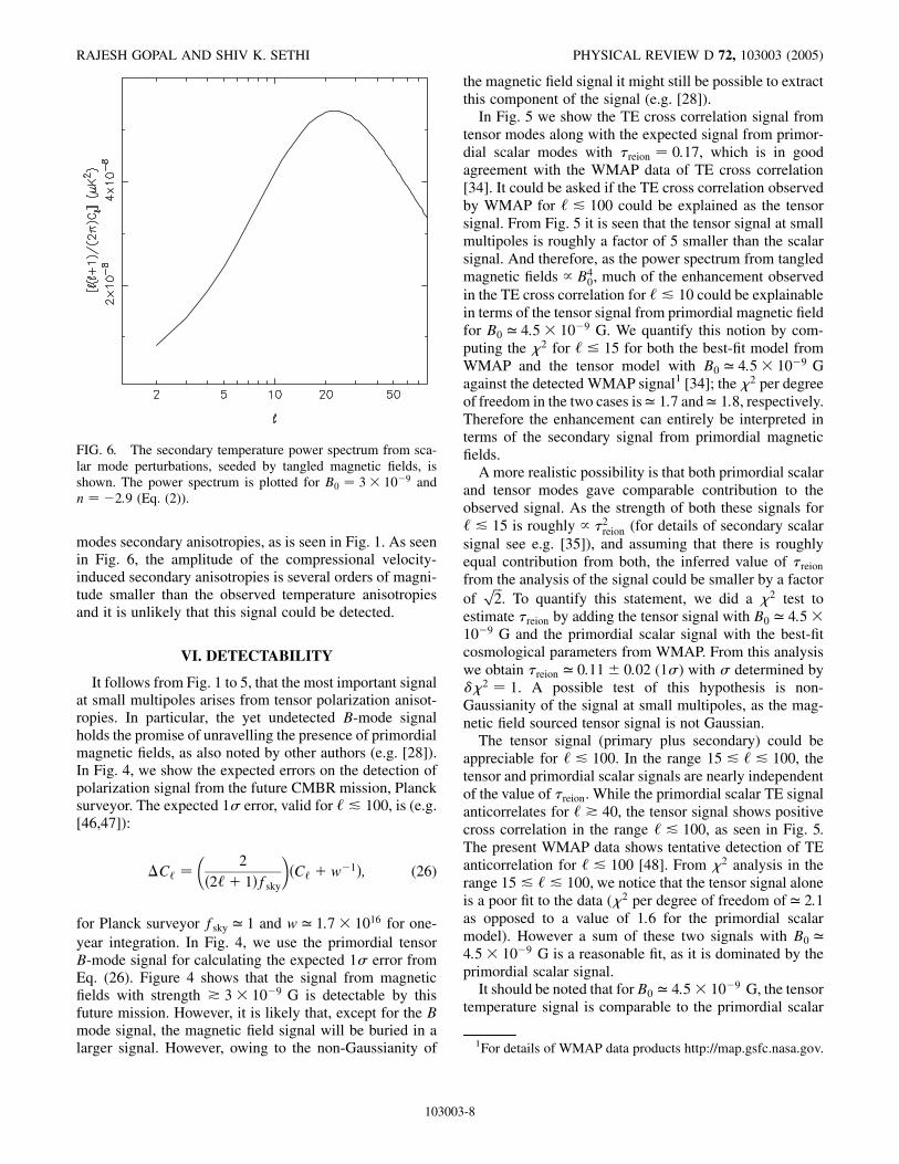
FIG. 6. The secondary temperature power spectrum from sca-lar mode perturbations, seeded by tangled magnetic fields, isshown. The power spectrum is plotted for B0 � 3� 10�9 andn � �2:9 (Eq. (2)).

RAJESH GOPAL AND SHIV K. SETHI PHYSICAL REVIEW D 72, 103003 (2005)

modes secondary anisotropies, as is seen in Fig. 1. As seenin Fig. 6, the amplitude of the compressional velocity-induced secondary anisotropies is several orders of magni-tude smaller than the observed temperature anisotropiesand it is unlikely that this signal could be detected.

1For details of WMAP data products http://map.gsfc.nasa.gov.

VI. DETECTABILITY

It follows from Fig. 1 to 5, that the most important signalat small multipoles arises from tensor polarization anisot-ropies. In particular, the yet undetected B-mode signalholds the promise of unravelling the presence of primordialmagnetic fields, as also noted by other authors (e.g. [28]).In Fig. 4, we show the expected errors on the detection ofpolarization signal from the future CMBR mission, Plancksurveyor. The expected 1� error, valid for ‘ & 100, is (e.g.[46,47]):

�C‘ ��

2

�2‘� 1�fsky

��C‘ � w

�1�; (26)

for Planck surveyor fsky ’ 1 and w ’ 1:7� 1016 for one-year integration. In Fig. 4, we use the primordial tensorB-mode signal for calculating the expected 1� error fromEq. (26). Figure 4 shows that the signal from magneticfields with strength * 3� 10�9 G is detectable by thisfuture mission. However, it is likely that, except for the Bmode signal, the magnetic field signal will be buried in alarger signal. However, owing to the non-Gaussianity of

103003

the magnetic field signal it might still be possible to extractthis component of the signal (e.g. [28]).

In Fig. 5 we show the TE cross correlation signal fromtensor modes along with the expected signal from primor-dial scalar modes with �reion � 0:17, which is in goodagreement with the WMAP data of TE cross correlation[34]. It could be asked if the TE cross correlation observedby WMAP for ‘ & 100 could be explained as the tensorsignal. From Fig. 5 it is seen that the tensor signal at smallmultipoles is roughly a factor of 5 smaller than the scalarsignal. And therefore, as the power spectrum from tangledmagnetic fields / B4

0, much of the enhancement observedin the TE cross correlation for ‘ & 10 could be explainablein terms of the tensor signal from primordial magnetic fieldfor B0 ’ 4:5� 10�9 G. We quantify this notion by com-puting the �2 for ‘ 15 for both the best-fit model fromWMAP and the tensor model with B0 ’ 4:5� 10�9 Gagainst the detected WMAP signal1 [34]; the �2 per degreeof freedom in the two cases is ’ 1:7 and ’ 1:8, respectively.Therefore the enhancement can entirely be interpreted interms of the secondary signal from primordial magneticfields.

A more realistic possibility is that both primordial scalarand tensor modes gave comparable contribution to theobserved signal. As the strength of both these signals for‘ & 15 is roughly / �2

reion (for details of secondary scalarsignal see e.g. [35]), and assuming that there is roughlyequal contribution from both, the inferred value of �reion

from the analysis of the signal could be smaller by a factorof

���2p

. To quantify this statement, we did a �2 test toestimate �reion by adding the tensor signal with B0 ’ 4:5�10�9 G and the primordial scalar signal with the best-fitcosmological parameters from WMAP. From this analysiswe obtain �reion ’ 0:11� 0:02 (1�) with � determined by��2 � 1. A possible test of this hypothesis is non-Gaussianity of the signal at small multipoles, as the mag-netic field sourced tensor signal is not Gaussian.

The tensor signal (primary plus secondary) could beappreciable for ‘ & 100. In the range 15 & ‘ & 100, thetensor and primordial scalar signals are nearly independentof the value of �reion. While the primordial scalar TE signalanticorrelates for ‘ * 40, the tensor signal shows positivecross correlation in the range ‘ & 100, as seen in Fig. 5.The present WMAP data shows tentative detection of TEanticorrelation for ‘ & 100 [48]. From �2 analysis in therange 15 & ‘ & 100, we notice that the tensor signal aloneis a poor fit to the data (�2 per degree of freedom of ’ 2:1as opposed to a value of 1:6 for the primordial scalarmodel). However a sum of these two signals with B0 ’4:5� 10�9 G is a reasonable fit, as it is dominated by theprimordial scalar signal.

It should be noted that for B0 ’ 4:5� 10�9 G, the tensortemperature signal is comparable to the primordial scalar

-8

TANGLED MAGNETIC FIELDS AND CMBR SIGNAL . . . PHYSICAL REVIEW D 72, 103003 (2005)

signal (Fig. 3). WMAP analysis obtained an upper limit of’ 0:7 on the ratio of tensor to scalar signal ([30]). Whilethis limit is rather weak, a more detailed analysis of thetemperature signal including the effect of tensor modesignal sourced by primordial magnetic fields might giveindependent constraints on the strength of primordial mag-netic fields.

In our �2 analysis we use only the diagonal componentsof the Fisher matrix. However, owing to incomplete sky,the signal is correlated, especially for small multipoles,across neighboring multipoles. However, a more compre-hensive analysis taking into this correlation is likely toyield similar conclusions for the reasons stated above.

Our conclusions are not too sensitive to the value ofsmall scale cutoff kmax or the scale of the filter kc used todefine the normalization (Eq. (2)) for magnetic field powerspectrum index n � �2:9 we use throughout the paper. Forkmax � kc � 0:05 Mpc�1, the foregoing discussion relatedto tensor mode anisotropies would be valid for B0 ’ 5�10�9 G. Therefore, the results for TE cross correlationfrom tensor perturbations can be interpreted to put boundson magnetic fields for only large scales k & 0:05 Mpc�1.

The strongest bound on primordial magnetic fields arisesfrom tensor perturbations in the prerecombination era [49].These bounds are weakest for nearly scale-invariant (n ’�3) magnetic fields power spectrum (Eq. (33) of [49]) andlargely motivated the choice of the power spectral index weconsider here. For n � �2:9, the bound obtained by [49] isconsiderably weaker than B0 ’ 4:5� 10�9 G, the valuesof interest to us in this paper. Vector modes might leaveobservable signature in the temperature and polarizationsignal for ‘ * 2000; the current observations give weakbound of B0 & 8� 10�9 G [28]. Tangled magnetic fieldsourced primary scalar temperature signal gives evenweaker bounds [50]. More recently, Chen et al. [51] ob-tained, from WMAP data analysis, a limit of & 10�8 G onthe primordial magnetic field strength for nearly scale-invariant spectra we consider here; [51] consider vector-mode temperature signal in their analysis and study pos-sible non-Gaussianity in the WMAP data. Another strongconstraint on large scale tangled magnetic fields comesfrom Faraday rotation of high redshift radio sources (seee.g [3]); this constraint is also weaker than the value ofmagnetic field required to explain the enhancement of theTE cross -correlation signal as seen by WMAP [19].Another interesting bound on the strength of tangled mag-netic fields during the reionization epoch arises from theZeeman splitting of 21 cm radiation from the epoch ofreionization [52]; this results in a bound on the magneticfield strength of & 100G coherent over megaparsecscales. Therefore, the value of B0 required to give appre-ciable contribution to the TE signal is well within the upperlimits on B0 from other considerations.

It should be noted that the entire foregoing discussion onthe tangled magnetic field tensor signal can be mapped to

103003

primordial tensor modes. The reason for this assertion isthat magnetic fields source tensor modes only prior to theepoch of neutrino decoupling, and the subsequent evolu-tion is source free, which is similar to the primordial tensormodes which are generated only during the inflationaryepoch and evolve without sources at subsequent times.Therefore, an analysis similar to ours could be used toput constraints on the relative strength of the tensor toscalar mode contribution (for a fixed scale) and the tensorspectral index of the primordial modes. The main obser-vational difference between such an interpretation and theone given here is that tensor signal sourced by magneticfields will not obey Gaussian statistics as opposed to theprimordial tensor modes.

VII. SUMMARY AND CONCLUSIONS

We have computed the secondary anisotropies from thereionization of the Universe in the presence of tangledprimordial magnetic fields. Throughout our analysis weuse the nearly scale-invariant magnetic field power spec-trum with n � �2:9. For vector modes, we compute thesecondary temperature and E- and B-mode polarizationautocorrelation signal. For scalar modes, the results forsecondary temperature angular power spectrum from com-pressional velocity modes are presented. For tensor modes,in addition to the secondary temperature and polarizationangular power spectra, we compute the TE cross correla-tion signal and compare it with the existing WMAP data;we also recompute the primary signal for tensor modes.Whenever possible we compare our results with the resultsexisting in the literature. In particular, Lewis [28] recentlycomputed fully numerically the vector and tensor primaryand secondary temperature and polarization power spectra.We compare our semianalytic results with this analysis andfind good agreement. Seshadri and Subramanian [36] com-puted the secondary temperature anisotropies from vectormodes. Our results are in good agreement with their con-clusion. Mack et al. [27] computed primary signal fromvector and tensor modes using the formalism we adopt inthis paper. Our results are in disagreement with their resultsfor ‘ * 75, and we have given reasons for our disagree-ment in the discussion above. In addition to comparisonwith existing literature, we also give new results for sec-ondary TE cross correlation from tensor modes and sec-ondary temperature angular power spectrum from scalarmodes.

We discuss below the details of expected signal fromeach of the perturbation mode:

Vector modes: The secondary temperature and polariza-tion signals from the vector modes is shown in Fig. 1 and 2.The secondary temperature signal increases / ‘2:4 for ‘ *

50 and reaches a value ’ 0:1�k�2 for ‘ ’ 104, in agree-ment with the analysis of [36]. For small ‘ the signal isvery small ( & 10�4�k�2) and for large ‘ the secondarysignal is smaller than the primary signal (e.g. [28]) and

-9

RAJESH GOPAL AND SHIV K. SETHI PHYSICAL REVIEW D 72, 103003 (2005)

therefore it is unlikely that the signature of reionizationcould be detected in the vector-mode temperature anisot-ropies. The polarization signal, shown in Fig. 2, is sourcedby the free streaming of dipole at the epoch of recombina-tion. This signal dominates the primary signal for ‘ & 10,but is several orders of magnitude smaller than the ex-pected signal from tensor modes.

Scalar modes: We only compute the secondary tempera-ture anisotropies from compressional velocity modes inthis case. As seen in Fig. 6, this contribution is severalorders of magnitude smaller than the already-detectedprimary signal and therefore its effects are unlikely to bedetectable.

Tensor modes: As seen from Figs. 4 and 5, the mostinteresting CMBR anisotropy signal for ‘ & 100 is fromthese modes. The secondary B-mode signal from tensormodes is detectable by future CMBR mission Planck sur-veyor for B0 ’ 3� 10�9 G . The tensor TE cross correla-tion from primordial magnetic fields can explain theobserved enhancement of the observed signal for ‘ & 10by WMAP for B0 ’ 4:5� 10�9 G if the primordial mag-netic fields are generated during the epoch of inflation.Assuming that tensor modes make a significant contribu-tion to the observed enhancement, the bounds on theoptical depth to the surface of reionization �reion are weakerby roughly a factor of

���2p

. This hypothesis can be borne/ruled out by testing the Gaussianity of the signal for ‘ &

10.

ACKNOWLEDGMENTS

We would like to thank A. Lewis for prompt reply to ourqueries and to T. R. Seshadri and K. Subramanian foruseful discussion.

APPENDIX A

In this section, we briefly discuss the terminology andpresent the complete expressions for the vector and tensorpower spectra �V�k� and �T�k� [27]. The energy-momentum tensor for magnetic fields for a single Fouriermode is a convolution of different Fourier modes and isgiven by:

Tij�k��Zd3q

�~Bi�q� ~Bj�k�q��

1

2�ij ~Bm�q� ~Bm�k�q�

�:

(A1)

The energy-momentum tensor has nonvanishing scalar,vector, and tensor components. The vector and tensorcomponents, in Fourier space, are defined as:

�Vi � PipkqTpq; (A2)

�Tij �

�PipPjq �

1

2PijPpq

�Tpq: (A3)

Here Pij � �ij � kikj. The vector and tensor anisotropic

103003

stress are then defined as the two-point correlations of theabove components as:

h�Vi �k��

Vi �k

0�i 2j��V��k�j2��k� k0�; (A4)

h�Tij�k��

Tij�k

0�i 4j��T��k�j2��k� k0�: (A5)

By evaluating the above correlations as also given in [27],we can arrive at the following approximate expression forthe power spectra for n <�3=2,

j�V�k�j2 �

A2

64�4�n� 3�k2n�3; (A6)

j�T�k�j2 �

2A2

64�4�n� 3�k2n�3: (A7)

Here, A is the normalization of the magnetic power spec-trum given in Eq. (2).

1. Bessel functions

We give below a list of all the relevant spherical Besselfunctions we have used in the foregoing text. These aretaken from Ref. [32]. For the vector-mode temperatureanisotropies, the relevant spherical Bessel functions are:

j�11�‘ �

������������������‘�‘� 1�

2

sj‘�x�x

; (A8)

j�21�‘ �

��������������������3‘�‘� 1�

2

sddx

�j‘�x�x

�: (A9)

For vector-induced polarization anisotropies, the sphericalBessel functions of interest are:

�v‘ �

1

2

�������������������������������‘� 1��‘� 2�

p �j‘�x�

x2 �j0‘�x�

x

�; (A10)

�v‘ �

1

2

�������������������������������‘� 1��‘� 2�

p j‘�x�x

: (A11)

Here prime denotes a derivative with respect to x. Fortensor-induced temperature and polarization anisotropies,the relevant Bessel functions are:

j�22�‘ �

��������������������3�‘� 2�!

8�‘� 2�!

sj‘�x�

x2 ; (A12)

�T‘ �

1

2

�j0‘�x� �

2j‘�x�x

�; (A13)

�T‘ �

1

4

��j‘�x� � j

00‘ �x� �

2j‘�x�

x2 �4j0‘�x�

x

�: (A14)

For scalar modes, the Bessel function of interest for

-10

TANGLED MAGNETIC FIELDS AND CMBR SIGNAL . . . PHYSICAL REVIEW D 72, 103003 (2005)

velocity-induced perturbations is:

j�10�‘ � j0‘�x�: (A15)

APPENDIX B

Gravitational waves correspond to transverse, tracelessperturbations to the metric: �gij � 2a2���hij with hii �kihij � 0. Since hij is a stochastic variable we can defineits power spectrum as:

hhij�k; ��hij�k0; ��i � 4jh�k; ��j2��k� k0�: (B1)

The evolution of hij then follows from the tensor Einsteinequation (see e.g. [32])

�h� 2_aa

_h� k2h � 8�GS�k; ��: (B2)

The source on the right-hand side (RHS) is the tensoranisotropic stress of the plasma which is defined as:S�k; �� � �T�k�=a2 (Eq. (A5)). We assume that the pri-mordial magnetic fields are generated by some mechanismat a very early epoch �in. It was recently shown by Lewis[28] that after the neutrino-decoupling epoch �? the neu-trino start free streaming and develop significant aniso-tropic stress which cancel the anisotropic stress of theprimordial magnetic fields to the leading order for super-horizon modes, resulting in negligible net anisotropicstress in the plasma. We can thus assume that for ���?, S�k; �� � 0 and for �� �?, S�k; �� � �T�k�=a2

where �T�k� is the magnetic tensor anisotropic stress asdefined in Eq. (A5). We now derive the solutions toEq. (B2) in various regimes. The evolution of the scalefactor a��� is given by the Friedmann equation:

_a 2 � H20��ma�� ��� ���a4�: (B3)

Here, �m;;�;� are the fractional densities in matter, radia-tion, neutrinos, and cosmological constant, respectively.Approximate solutions in the radiation-dominated and

matter-dominated epoch are a��� � 2�����������������

�m

q��0

anda��� � � ��0

�2, respectively. Using the above form for thescale factor we can rewrite Eq. (B2) for �in < � < �? as:

�h�2

�_h� k2h �

3R�T�k�

�

1

�2 : (B4)

Here, R � �=�� ���� ’ 0:6. � is the CMBR en-ergy density. Equation (B4) can be solved exactly using theGreen’s function technique to give [27]:

h�k; �� �3R�T�k�

�

Z �

�ind�0

sink��� �0���0

: (B5)

For superhorizon modes k�� 1, the above form can besimplified to give:

103003

h�k; �� �3R�T�k�

�

Z �

�ind�0

k��� �0�k��0

�3R�T�k�

�ln���in

�: (B6)

For �� �?, the evolution of h is given by the homoge-neous solutions in the radiation and matter-dominatedregimes:

hrad�k; �� � A1j0�k��; (B7)

hmat�k; �� � A2j1�k��k�

: (B8)

The coefficients A1 and A2 are determined by matching thesuperhorizon solutions at the two transitions �? and �eq.We thus get

A2 � 3A1 �9R�T�k�

�ln��?�in

�: (B9)

Thus, the full expression for the matter-dominated solutioncan be written as:

_h mat��; k� �9R�T�k�

�ln��?�in

�j2�k���

: (B10)

This solution is used for solving tensor temperature andpolarization primary and secondary anisotropies. Few as-sumptions have been made in deriving the above expres-sion. First, the transition between radiation-dominated tomatter-dominated region has been assumed to be instanta-neous. This however does not affect the evolution of modeswith wavelength greater than the width of transitionk�eq & 1. Moreover, only superhorizon solutions havebeen used to match the solutions for h at different transi-tions. These simplifications however do not affect theresults quotes for small multipoles as discussed in themain section.

1. Tight-coupling tensor quadrupole

In the tight-coupling regime z * 1100 to lowest order inmean-free path, we have PT � � _h=�3 _�� [27]. We howeveruse the expression accurate to the second order in mean-free path as is done for the scalar modes in [53]. Using theBoltzmann equation for the evolution of tensor modes weget the following equation for PT�k; �� in the tight-coupling limit:

_P�3

10_�P � �

_h10: (B11)

The lowest order solution to this equation is obtained byneglecting the _P in the equation, which gives P �� _h=�3 _��. The above equation however can be solved ex-actly to give:

P��� �Z �

0d�0 _he��3=10����0�������: (B12)

We use the standard recombination history for computing�.

-11

RAJESH GOPAL AND SHIV K. SETHI PHYSICAL REVIEW D 72, 103003 (2005)

[1] E. N. Parker, Cosmical Magnetic Fields: Their Origin andtheir Activity (Clarendon, Oxford, 1979).

[2] I. B. Zeldovich, A. A. Ruzmaikin, and D. D. Sokolov, TheFluid Mechanics of Astrophysics and Geophysics, Vol. 3(Gordon and Breach, New York, 1983),p. 381.

[3] L. M. Widrow, Rev. Mod. Phys. 74, 775 (2002).[4] K. -T. Kim, P. P. Kronberg, G. Giovannini, and T. Venturi,

Nature (London) 341, 720 (1989).[5] A. A. Ruzmaikin, A. M. Shukurov, and D. D. Sokoloff,

Magnetic Fields of Galaxies (Kluwer, Dordrecht, 1988).[6] A. Shukurov, in Mathematical Aspects of Natural

Dynamos, edited by E. Dormy (Kluwer, Dordrecht, 2004).[7] E. R. Harrison, Mon. Not. R. Astron. Soc. 147, 279

(1970).[8] K. Subramanian, D. Narasimha, and S. M. Chitre, Mon.

Not. R. Astron. Soc. 271, L15 (1994).[9] R. M. Kulsrud, R. Cen, J. P. Ostriker, and D. Ryu,

Astrophys. J. 480, 481 (1997).[10] D. Grasso and H. R. Rubinstein, Phys. Rep. 348, 163

(2001).[11] R. Gopal and S. K. Sethi, astro-ph/0411170.[12] S. Matarrese, S. Mollerach, A. Notari, and A. Riotto, Phys.

Rev. D 71, 043502 (2005).[13] M. S. Turner and L. M. Widrow, Phys. Rev. D 37, 2743

(1988).[14] B. Ratra, Astrophys. J. Lett. 391, L1 (1992).[15] M. Giovannini, Int. J. Mod. Phys. D 13, 391 (2004).[16] I. Wasserman, Astrophys. J. 224, 337 (1978).[17] E. Kim, A. V. Olinto, and R. Rosner Astrophys. J. 468, 28

(1996).[18] K. Subramanian and J. D. Barrow, Phys. Rev. D 58,

083502 (1998).[19] S. K. Sethi, Mon. Not. R. Astron. Soc. 342, 962 (2003).[20] R. Gopal and S. K. Sethi, J. Astrophys. Astron. 24, 51

(2003).[21] S. K. Sethi and K. Subramanian, Mon. Not. R. Astron.

Soc. 356, 778 (2005).[22] J. D. Barrow, P. G. Ferreira, and J. Silk, Phys. Rev. Lett.

78, 3610 (1997).[23] K. Subramanian and J. D. Barrow, Phys. Rev. Lett. 81,

3575 (1998).[24] K. Subramanian and J. D. Barrow, Mon. Not. R. Astron.

Soc. 335, L57 (2002).[25] R. Durrer, P. G. Ferreira, and T. Kahniashvili, Phys. Rev. D

61, 043001 (2000).

103003

[26] T. R. Seshadri and K. Subramanian, Phys. Rev. Lett. 87,101301 (2001).

[27] A. Mack, T. Kahniashvili, and A. Kosowsky, Phys. Rev. D65, 123004 (2002).

[28] A. Lewis, Phys. Rev. D 70, 043011 (2004).[29] W. Hu and S. Dodelson, Annu. Rev. Astron. Astrophys.

40, 171 (2002).[30] D. N. Spergel, Astrophys. J. Suppl. Ser. 148, 175 (2003).[31] M. Tegmark et al., Phys. Rev. D 69, 103501 (2004).[32] W. Hu and M. White, Phys. Rev. D 56, 596 (1997).[33] J. M. Kovac, E. M. Leitch, C. Pryke, J. E. Carlstrom, N. W.

Halverson, and W. L. Holzapfel, Nature (London) 420,772 (2002).

[34] A. Kogut et al., Astrophys. J. Suppl. Ser. 148, 161 (2003).[35] M. Zaldarriaga, Phys. Rev. D 55, 1822 (1997).[36] T. R. Seshadri and K. Subramanian, Phys. Rev. D 72,

023004 (2005).[37] S. Perlmutter et al., Astrophys. J. 517, 565 (1999).[38] A. G. Riess et al., Astrophys. J. 607, 665 (2004).[39] D. Tytler, J. M. O’Meara, N. Suzuki, and D. Lubin, Phys.

Rep. 333, 409 (2000).[40] W. L. Freedman et al., Astrophys. J. 553, 47 (2001).[41] K. Jedamzik, V. Katalinic and A. V. Olinto, Phys. Rev. D

57, 3264 (1998).[42] L. D. Landau and E. M. Lifshitz, Fluid Mechanics

(Pergamon, New York, 1987).[43] K.-W. Ng and A. D. Speliotopolous, Phys. Rev. D 52, 2112

(1995).[44] S. Dodelson and J. M. Jubas, Astrophys. J. 439, 503

(1995).[45] E. Vishniac, Astrophys. J. 322, 597 (1987).[46] M. Zaldarriaga, D. N. Spergel, and U. Seljak, Astrophys. J.

488, 1 (1997).[47] S. Prunet, S. K. Sethi, and F. Bouchet, Mon. Not. R.

Astron. Soc. 314, 348 (2000).[48] H. V. Peiris et al., Astrophys. J. Suppl. Ser. 148, 213

(2003).[49] C. Caprini and R. Durrer, Phys. Rev. D 65, 023517 (2002).[50] S. Koh and C. H. Lee, Phys. Rev. D 62, 083509 (2000).[51] G. Chen, P. Mukherjee, T. Kahniashvili, B. Ratra, and Y.

Wang, Astrophys. J. 611, 655 (2004).[52] A. Cooray and S. R. Furlanetto, Mon. Not. R. Astron. Soc.

359, 47 (2005).[53] M. Zaldarriaga and D. D. Hariri, Phys. Rev. D 52, 3276

(1995).

-12