
Tampereen teknillinen yliopisto. Julkaisu 1229 - TUT · Tampereen teknillinen yliopisto. Julkaisu...
124
Transcript of Tampereen teknillinen yliopisto. Julkaisu 1229 - TUT · Tampereen teknillinen yliopisto. Julkaisu...


Tampereen teknillinen yliopisto. Julkaisu 1229 Tampere University of Technology. Publication 1229
Jussi Turkka
Aspects of Knowledge Mining on Minimizing Drive Tests in Self-organizing Cellular Networks
Thesis for the degree of Doctor of Science in Technology to be presented with due permission for public examination and criticism in Tietotalo Building, Auditorium TB109, at Tampere University of Technology, on the 22nd of August 2014, at 12 noon.
Tampereen teknillinen yliopisto - Tampere University of Technology Tampere 2014

ISBN 978-952-15-3332-7 (printed) ISBN 978-952-15-3401-0 (PDF) ISSN 1459-2045

Doctoral advisor
Professor Jukka Lempiäinen
Department of Communications Engineering
Tampere University of Technology
Tampere, Finland
Second advisor
Professor Tapani Ristaniemi
Department of Mathematical Information Technology
University of Jyväskylä
Jyväskylä, Finland
Pre-examiner
Assistant Director, Ph.D. Seppo Hämäläinen
Ooredoo Group
Doha, Qatar
Pre-examiner and opponent
Head of the Institute, Professor Petri Mähönen
Institute for Networked Systems
RWTH Aachen University
Aachen, Germany
Opponent
Head of Department, Professor Riku Jäntti
Department of Communications and Networking
Aalto University
Helsinki, Finland


I
Abstract
he demand for mobile data traffic is about to explode and this drives operators to find ways
to further increase the offered capacity in their networks. If networks are deployed in the
traditional way, this traffic explosion will be addressed by increasing the number of network
elements significantly. This is expected to increase the costs and the complexity of planning,
operating and optimizing the networks. To ensure effective and cost-efficient operations, a higher
degree of automation and self-organization is needed in the next generation networks. For this
reason, the concept of self-organizing networks was introduced in LTE covering multitude of use
cases. This was specifically done in the areas of self-configuration, self-optimization and self-
healing of networks. From an operator’s perspective, automated collection and analysis of field
measurements while complementing the traditional drive test campaigns is one of the top use
cases that can provide significant cost savings in self-organizing networks.
This thesis studies the Minimization of Drive Tests in self-organizing cellular networks from
three different aspects. The first aspect is network operations, and particularly the network fault
management process, as the traditional drive tests are often conducted for troubleshooting
purposes. The second aspect is network functionality, and particularly the technical details about
the specified measurement and signaling procedures in different network elements that are needed
for automating the collection of the field measurement data. The third aspect concerns the analysis
of the measurement databases that is a process used for increasing the degree of automation and
self-awareness in the networks, and particularly the mathematical means for autonomously
finding meaningful patterns of knowledge from huge amounts of data. Although the above
mentioned technical areas have been widely discussed in previous literature, it has been done
separately and only a few papers discuss how for example, knowledge mining is employed for
processing field measurement data in a way that minimizes the drive tests in self-organizing LTE
networks.
The objective of the thesis is to use well known knowledge mining principles to develop
novel self-healing and self-optimization algorithms. These algorithms analyze MDT databases to
detect coverage holes, sleeping cells and other geographical areas of anomalous network
behavior. The results of the research suggest that by employing knowledge mining in processing
the MDT databases, one can acquire knowledge for discriminating between different network
problems and detecting anomalous network behavior. For example, downlink coverage
optimization is enhanced by classifying RLF reports into coverage, interference and handover
problems. Moreover, by incorporating a normalized power headroom report with the MDT
T

II
reports, better discrimination between uplink coverage problems and the parameterization
problems is obtained. Knowledge mining is also used to detect sleeping cells by means of
supervised and unsupervised learning. The detection framework is based on a novel approach
where diffusion mapping is used to learn about network behavior in its healthy state. The sleeping
cells are detected by observing an increase in the number of anomalous reports associated with a
certain cell. The association is formed by correlating the geographical location of anomalous
reports with the estimated dominance areas of the cells.
Moreover, RF fingerprint positioning of the MDT reports is studied and the results suggest
that RF fingerprinting can provide a quite detailed location estimation in dense heterogeneous
networks. In addition, self-optimization of the mobility state estimation parameters is studied in
heterogeneous LTE networks and the results suggest that by gathering MDT measurements and
constructing statistical velocity profiles, MSE parameters can be adjusted autonomously, thus
resulting in reasonably good classification accuracy.
The overall outcome of the thesis is as follows. By automating the classification of the
measurement reports between certain problems, network engineers can acquire knowledge about
the root causes of the performance degradation in the networks. This saves time and resources
and results in a faster decision making process. Due to the faster decision making process the
duration of network breaks become shorter and the quality of the network is improved. By taking
into account the geographical locations of the anomalous field measurements in the network
performance analysis, finer granularity for estimating the location of the problem areas can be
achieved. This can further improve the operational decision making that guides the corresponding
actions for example, where to start the network optimization. Moreover, by automating the time
and resource consuming task of tuning the mobility state estimation parameters, operators can
enhance the mobility performance of the high velocity UEs in heterogeneous radio networks in a
cost-efficient and backward compatible manner.

III
Preface
he research work for the thesis was done during between 2009 and 2013 when I had an
opportunity to work at Magister Solutions Ltd. Honestly speaking, without the encouraging
and innovative working environment, I would not have had the dedication and energy for
accomplishing this scientific excursion alongside my daily duties. I would like to thank all my
Magister colleagues at Tampere, Jyväskylä and Helsinki, and especially Dr. Janne Kurjenniemi
(CEO), Dr. Timo Nihtilä, Dr. Jani Puttonen and Dr. Kari Aho.
I would like to express my sincere appreciation to my doctoral advisors, Professor Jukka
Lempiäinen from the Department of Communications Engineering at Tampere University of
Technology and Professor Tapani Ristaniemi from the Department of Mathematical Information
Technology at the University of Jyväskylä, for the opportunity to work under their guidance. I
want to dedicate special thanks to Professor Amir Averbuch from the School of Computer Science
at Tel-Aviv University and Dr. Gil David for introducing me to the concept of anomaly detection.
Moreover, I would also like to thank all of my co-authors, Dr. Olli Alanen, Mr. Tero Henttonen,
Mr. Fedor Chernogorov, Mr. Kimmo Brigatti and Mr. Andreas Lobinger, for making valuable
contributions to the publications that this thesis is compiled from.
In addition to the support from the Department of Communications Engineering (Thank You
Prof. Mikko Valkama and Prof. Markku Renfors), the work was financially supported by the
University of Jyväskylä, the Tampere Doctoral Program in Information Science and Engineering
(TISE), Tekniikan edistämissäätiö (TES), Elektroniikka Insinöörien Seura (EIS) and the Ulla
Tuominen Foundation.
Moreover, I want to thank the doctors and former members of the Radio Network Group at
Tampere University of Technology, Dr. Jarno Niemelä, Dr. Jakub Borkowski, Dr. Panu
Lähdekorpi, Dr. Tero Isotalo, Mr. Muhammed Ushan Sheik and Mr. Teemu Pesu, for all the
innovative discussions, feedback and criticism that they gave me when it was needed and seen
appropriate. In addition, I want to thank Mr. Jaakko Penttinen for his views and hands-on
experience about manual drive tests in the field of network troubleshooting. I am also grateful for
the various informal tea-table discussions with Mr. Jukka Talvitie, Mr. Toni Levanen, Mr. Tero
Kuosmanen, Mr. Kari Hämäläinen, and many former co-workers, senior co-workers and line
managers at Nokia, Nokia Siemens Networks and Renesas Mobile Europe Ltd.
T

IV
I want to thank my parents Tuomo and Ulla, and my brothers, Jaakko, Joonas and Jesse,
for their support and the time we have spent together at Jurkkola over the years. Family is the
most important thing that one can have throughout life time. Finally, I want to thank my beloved
wife Orvokki for all the love and care at home, and our young offspring Ossi, for spontaneously
re-organizing my papers and my thoughts from time to time while I was writing the thesis. It has
been fun.
Tampere, Finland
August 2014.
Jussi Taneli Turkka

V
Table of Contents
Abstract .......................................................................................................................................... I
Preface ......................................................................................................................................... III
List of Publications .................................................................................................................... VII
List of Abbreviations ................................................................................................................... IX
List of Symbols ............................................................................................................................. X
List of Figures ............................................................................................................................ XII
1. Introduction ............................................................................................................................... 1
1.1 Background and Motivation ................................................................................................ 1
1.2 Scope and Objectives of the Thesis .................................................................................... 3
1.3 Main Results of the Thesis .................................................................................................. 4
1.4 Author’s Original Contribution ........................................................................................... 5
1.5 Organization of the Thesis .................................................................................................. 6
2. Operation of Modern Cellular Radio Network.......................................................................... 9
2.1 The Economics of the Radio Networks............................................................................... 9
2.2 Radio Network Architecture ............................................................................................. 11
2.3 Operating the Radio Network ........................................................................................... 13
2.3.1 Radio Network Planning ............................................................................................ 13
2.3.2 Radio Network Monitoring ........................................................................................ 14
2.3.3 Radio Network Optimization ..................................................................................... 16
2.3.4 Radio Network Fault Management ............................................................................ 17
2.4 Operation and Management Vision for Future Radio Networks ...................................... 18
3. Concept of Self-Organizing Networks .................................................................................... 19
3.1 Self-Organizing Networks ................................................................................................ 19
3.1.1 Self-Configuration ..................................................................................................... 22
3.1.2 Self-Optimization ....................................................................................................... 23
3.1.3 Self-Healing ............................................................................................................... 24

VI
3.2 Minimization of Drive Tests ............................................................................................. 25
3.2.1 MDT Architecture ...................................................................................................... 27
3.2.3 MDT Measurements .................................................................................................. 29
4. Means and Methods for Supporting Network Self-Organization ............................................ 31
4.1 Autonomic Control Function ............................................................................................ 31
4.2 Principles of Knowledge Mining ...................................................................................... 33
4.2.1 Classification .............................................................................................................. 33
4.2.2 Clustering ................................................................................................................... 34
4.2.3 Anomaly Detection .................................................................................................... 35
4.2.4 Dimensionality Reduction .......................................................................................... 37
5. Knowledge Mining Assisted Network Performance Improvements ....................................... 39
5.1 Coverage Optimization with Extended RLF Reports ....................................................... 39
5.2 Smart Discrimination of Uplink Coverage Problems ....................................................... 41
5.3 MDT assisted Sleeping Cell Detection ............................................................................. 43
5.3.1 Clustering based approach for Sleeping Cell Detection............................................. 44
5.3.2 Classification based Approach for Sleeping Cell Detection ...................................... 46
5.4 Localization of MDT Radio Measurements ...................................................................... 50
5.4.1 Performance in various intra- and inter-frequency network deployments ................. 51
5.4.2 Performance constraints by 3GPP cell detection performance requirements ............ 52
5.5 MDT assisted Self-Optimization of UE Mobility State .................................................... 54
6. Conclusion ............................................................................................................................... 57
6.1 Concluding Summary ....................................................................................................... 57
6.2 Future Work ...................................................................................................................... 58
Appendix A: Dynamic System Simulator ................................................................................... 61
Bibliography ................................................................................................................................ 65
Original Papers ............................................................................................................................ 73

VII
List of Publications
This thesis is a compilation of the following publications
[P1] Turkka J. and Lobinger A., “Non-regular Layout for Cellular Network System
Simulations”, published in Proceeding of 21st IEEE International Symposium on
Personal, Indoor and Mobile Radio Communications (PIMRC), September 2010,
Istanbul, Turkey.
[P2] Puttonen J., Turkka J., Alanen O. and Kurjenniemi, ”Coverage Optimization for
Minimization of Drive Tests in LTE with Extended RLF Reporting”, published in
Proceeding of 21st IEEE International Symposium on Personal, Indoor and Mobile Radio
Communications (PIMRC), September 2010, Istanbul, Turkey.
[P3] Turkka J. and Puttonen J., “Using LTE Power Headroom Report for Coverage
Optimization”, published in Proceeding of 72nd IEEE Vehicular Technology Conference
(VTC-fall), September 2011, San Francisco, United States.
[P4] Chernogorov F., Turkka J., Ristaniemi T. and Averbuch A.,” Detection of Sleeping Cells
in LTE Networks Using Diffusion Maps”, published in Proceeding of International
Workshop on Self-Organizing Networks (IWSON), May 2011, Budapest, Hungary.
[P5] Turkka J., Chernogorov F., Brigatti K., Ristaniemi T. and Lempiäinen J., “An Approach
for Network Outage Detection from Drive Testing Databases”, published in Journal of
Computer Networks and Communications, vol. 2012, Article ID: 163184, 13 pages,
December 2012, doi:10.1155/2012/163184.
[P6] Mondal R., Turkka J., Ristaniemi T. and Henttonen T, ”Positioning in Heterogeneous
Small Cell Networks using MDT RF Fingerprints”, published in Proceedings of the First
IEEE International Black Sea Conference on Communications and Networking, July
2013, Batumi, Georgia.
[P7] Mondal R., Turkka J., Ristaniemi T. and Henttonen T., “Performance Evaluation of MDT
Assisted LTE RF Fingerprinting Framework”, published in Proceedings of 7th
International Conference on Mobile Computing and Ubiquitous Networking
(ICMU2014), January 2014, Singapore.
[P8] Turkka J., Henttonen T. and Ristaniemi T., “Self-optimization of LTE Mobility State
Estimation Thresholds”, published in Proceeding of IEEE International Conference on
Wireless Communications and Networking, Workshop on Self-Organizing Networks
(SONET), April 2014, Istanbul, Turkey.

VIII
VIII

IX
List of Abbreviations
5G 5th Generation of Mobile Networks
3GPP Third Generation Partnership Project
ANR Automatic Neighbor Relations
ARPU Average Revenue Per User
BS Base Station
BSC Base Station Controller
CAPEX Capital Expenditures
CART Classification And Regression Trees
CCO Coverage and Capacity Optimization
CGI Cell Global Identification
CN Core Network
CRS Cell-specific Reference Symbols
CS Circuit Switched
DM Diffusion Map
eNB Evolved NodeB
EPC Evolved Packet Core
E-UTRAN Evolved Universal Terrestrial Radio Access Network
FM Fault Management
GNSS Global Navigation Satellite System
GSM Global System for Mobile communications
HOF Handover Failure
HSPA High Speed Packet Access
ICIC Inter-Cell Interference Coordination
IMEI SV International Mobile Equipment Identifier and Software Version
IMS Internet Multimedia Services
IMSI International Mobile Subscriber Identifier
IP Internet Protocol
IPEX Investment Expenditures
KLD Kullback-Leibler Divergence
KNN k-Nearest Neighbors
KPI Key Performance Indicators
LTE Long Term Evolution
LTE-A LTE Advanced
MAD Mahalanobis Distance
MDT Minimization of Drive Tests
MIMO Multi-Input Multi-Output
MLB Mobility Load Balancing
MRO Mobility Robustness Optimization
MSE Mobility State Estimation
NB UTRAN NodeB
NGMN Next Generation Mobile Networks

X
OAM Operations, Administration and Maintenance architecture
OFDM Orthogonal Frequency-Division Multiplexing
OPEX Operational Expenditures
PCI Physical Cell Identifier
PHR Power Headroom Report
PM Performance Management
PRB Physical Resource Block
PS Packet Switched
QCI QoS Class Identifier
QoS Quality of Service
RACH Random Access Channel
RAN Radio Access Network
RAT Radio Access Technologies
RF Radio Frequency
RLF Radio Link Failure
RNC Radio Network Controller
RSRP Reference Symbol Received Power
RSRQ Reference Symbol Received Quality
RSSI Received Signal Strength Indicator
RRC Radio Resource Control
RRM Radio Resource Management
RXP Received Power
SINR Signal to Interference and Noise Ratio
SON Self-Organizing Networks
TCO Total Cost of Ownership
UL Uplink
UL-SCH Uplink Shared Channel for data transmission in LTE
UMTS Universal Mobile Telecommunication System
UTRAN Universal Terrestrial Radio Access Network
VoIP Voice over IP
WCQI Wideband Channel Quality Indictor
WLAN Wireless Local Area Network

X
List of Symbols
(.)T Transpose operation
tr(.) Trace operation
(.)-1 Matrix inverse operation
|.| Absolute value of a real number or a determinant operation of a matrix
Σp Covariance matrix for training data
Σq Covariance matrix for testing data
p Column vector of training data
q Column vector of testing data
de Euclidean distance
dm Mahalanobis distance
dkl Kullback-Leibler divergence
I Identity matrix
ρm Density metric for mth data sample
ηm Number of samples inside k-dimensional ball for mth data sample
zi Anomaly score for eNB i
xi Number of outage samples associated with eNB i
μL Sample mean of outage samples observed in set of eNBs
σL Sample deviation of outage samples observed in set of eNBs
ψl The lth Eigen vector of decomposed Markov’s transition matrix
ψl(xi) The lth entry of the right eigenvector for point xi
λl Eigenvalue of the lth eigenvector ψl
Dt2(.) Diffusion distance operation between two points
Ψt A matrix of diffusion coordinates
Ψt(xi) The ith row of Ψt providing the diffusion coordinates of xi
PCMAX UE Nominal Maximum Transmission Power
MPUSCH(i) UL-SCH PRB allocation for ith subframe
P0_PUSCH(j) Minimum transmission power level per PRB
α(j) Fractional pathloss compensation factor
ΔTF(i) Modulation and coding scheme dependent constant offset
f(i) Correction function to the UL power control mechanism
NCR Number of handovers and reselections during TCRmax
TCRmax Time duration for sliding time window
NCR_M NCR threshold between normal and medium mobility categories
NCR_H NCR threshold between medium and high mobility categories
X1 Distribution of NCR samples belonging to lower mobility category
X2 Distribution of NCR samples belonging to higher mobility category
μ1 Mean NCR value of distribution X1
σ1 Standard deviation of distribution X1
μ2 Mean value of distribution X2
σ2 Standard deviation of distribution X2
NTH Threshold between distributions X1 and X2

XI
Ês Energy per symbol
Iot Interference over thermal noise
leiu Radio link between eNB i and UE u for one resource element es,sc
es,sc Resource element indexed by subcarrier sc and OFDM symbol s
s Index for certain OFDM symbol in LTE transmission
sc Index for certain subcarrier in LTE transmission
pli(.) Distance diu dependent pathloss model
diu Distance between eNB i and UE u.
sfiu(.) Log-normal slow fading factor
|ffiu(.)|2 Average power of complex fast fading factor
gi(.) Antenna gain factor
φiu, Angular difference between eNB i antenna and UE in horizontal plane
θiu Angular difference between eNB i antenna and UE in vertical plane
rxeiu Received power per resource element
txei Transmitted power per resource element
rsrp(t) Instantaneous RSRP
S A set of indexes of OFDM symbols transmitting reference symbols
RSsN A set of subcarrier indexes transmitting CRS symbols during s
Ns Number of OFDM symbols transmitting reference symbols
NrsN Number of subcarriers transmitting CRS symbols on measurement
bandwidth
rsrpL1 Layer one RSRP measurement
Nw Number of instantaneous RSRP samples
w Sampling index in sliding time window
t Sampling period for instantaneous measurements
rsrpL3 Layer three RSRP measurement
rsrpL3_prev Previous layer three RSRP measurement
a L3 filtering variable
k Configurable filter coefficient
rsrq(t) Instantaneous RSRQ
rssi(t) Instantaneous RSSI
SCN A set of indexes of all subcarrier on measurement bandwidth
Ntx Number of radio links to eNBs
RSsW A set of subcarriers indexes of transmitting reference symbols during
s in whole transmission bandwidth
NrsW Number of subcarriers per OFDM symbol transmitting CRS symbols
in whole transmission bandwidth
wcqi(t) Instantaneous wideband CQI

XII
List of Figures
Figure 1: Trend for traffic and revenue in radio networks
Figure 2: Illustration of 3GPP radio network architecture
Figure 3: Procedure for operating a traditional radio network
Figure 4: Network monitoring tools
Figure 5: Manual network fault management process [22]
Figure 6: Operation of a Self-Organizing Network
Figure 7: Illustration of parameter and process interdependencies [15]
Figure 8: Overview of management-based MDT architecture
Figure 9: Block diagram for SON control process
Figure 10: Classification tree for RLF problems
Figure 11: Simulated network dominance areas
Figure 12: Number of anomalies per e-NB
Figure 13: Relative number of different outage samples
Figure 14: Anomaly scores in time before and after triggering the problem in eNB-8
Figure 15: Cumulative distribution functions of RF fingerprinting position error
Figure 16: Heterogeneous and regular macro network simulation scenarios
Figure 17: UE handover count distributions in a case where the sliding time window is 120s
Figure 18: System simulator architecture


“It is not the strongest of the species that survives, nor the most intelligent that survives. It
is the one that is the most adaptable to change.” – Charles Darwin
“It is not the strongest of the species that survives, nor the most intelligent that survives. It
is the one that is the most adaptable to change.” – Charles Darwin


1
1. Introduction
t was year 2012 and a small, light-weight and stylish cordless mobile phone is the de-facto
item that we all carry with us in all times. More than 21 years has passed since the first official
GSM (Global System for Mobile communications) call was made on Radiolinja’s network in
1991 and now we have more than 8.9 million mobile subscribers in Finland. In 2011, Finnish
mobile subscribers made more than 5.1 billion calls, sent more than 4.5 billion text messages and
transmitted more than 60 000 terabytes of data [1]. The technological success of the mobile
phones is unquestionable and life without one would be challenging, if not impossible. The mobile
business segment is becoming more and more popular and is growing every year. New
technologies, new applications and new services are offered to data hungry subscribers. Two
decades ago we had GSM, ten years ago we had UMTS (Universal Mobile Telecommunication
System) and today we have LTE (Long Term Evolution) and now, we are already paving the road
for the 5th generation (5G) technologies and the Internet of Things. Although the mobile phones
are the most visible evidence of this new technology, the high quality services with seamless
mobility performance always require the deployment of a sophisticated cellular network
infrastructure in the background. The popularity of the different mobile applications, services and
the rapid growth of the network usage create new challenges for service providers and operators
[2]. How do we provide the capacity that is needed to satisfy the increasing data demands of
subscribers while still maintaining the profitability of the mobile business?
1.1 Background and Motivation
For decades there have been three main design principles for increasing the capacity of wireless
systems. The principles are widening the system bandwidth, improving the spectral efficiency
and shortening the frequency reuse distance. The total system bandwidth and signal to noise
conditions define the upper bound for total system capacity according to the Shannon–Hartley
theorem. Therefore, the trend has been to increase the bandwidth when introducing new
generation of radio technologies. The maximum bandwidth in LTE is four times wider than the
bandwidth in UMTS. By aggregating carriers in LTE Advanced (LTE-A), even larger system
bandwidths can be achieved. Spectral efficiency on the other hand refers to the means to enhance
bandwidth usage by increasing the number of transmitted bits per second per unit of bandwidth.
Recent improvements in LTE spectral efficiency have been related to advanced multi antenna
transceivers for example, multi-input multi-output (MIMO) transceivers. These transceivers
provide remarkable capacity gains [3]. However, the whole concept of cellular networks relies on
reusing frequencies since only it allows deployment of continuous coverage for nationwide areas
I

2
with limited frequency resources. In principle, two base stations can use the same frequencies
simultaneously if they are isolated. One way to ensure this isolation is to have a large enough
separation distance between the base stations. By shortening the distance, the capacity and
frequency reuse rate increases, but the interference increases as well. If the interference can be
mitigated for example, by using higher frequencies; adjusting transmission power; optimizing
antenna configurations; or using advanced transceivers; then more base stations per unit area can
be deployed, thus increasing the total capacity. For the next generation of cellular networks, dense
small cell networks are envisioned to be one of the potential deployment strategies for addressing
the capacity crunch [4]. However, cell densification and the co-existence of several radio access
networks for example, GSM, UMTS and LTE, poses challenges for network vendors and
operators. In particular, it will be difficult to manage their complex network infrastructures in a
cost efficient way by using traditional methods while maintaining a good grade of service.
A fundamental planning principle of any radio network is to fulfill coverage, capacity and
quality targets as cost efficiently as possible [5], [6]. Traditionally, the cost-efficiency goal is
fulfilled by using the minimum number of base station sites because this minimizes the total cost
of the network. Cell densification means that capacity is increased by deploying a hundred or a
thousand times more small base stations. Hence, one of the challenges from an operator point of
view will be to ensure efficient operation and optimization of the all co-existing networks with
limited cost constraints. Even if the purchase cost of a small base station is reduced to the
minimum, the total cost of small cell networks can reach an unacceptable level if implementation
and operational expenditures (OPEX) cannot be reduced significantly. For this reason, the concept
of Self-Organizing Networks (SON) has been introduced in LTE [7].
The goal of the SON concept is to increase the degree of automation in the network
planning, configuration and optimization processes in order to increase efficiency while reducing
the costs of operating the networks. The cost savings in Capital Expenditures (CAPEX) are related
to better utilization of the network resources when increasing coverage, capacity and quality. If
this allows for new investments to be postponed, then the return of the investments in the existing
equipment improves and results in CAPEX savings. The OPEX savings are related to increasing
the productivity of the operator’s staff, for example by reducing the amount of repetitive and time
consuming optimization tasks. Although self-organization can reduce the amount of manual
intervention needed to carry out the optimization tasks, it also poses new challenges. It is expected
that the automation of complex network procedures that have intricate interdependencies will
require more feedback data to assist with the autonomous decision making with regards to the
network elements. In particular, the autonomous collection of the radio measurements for network
coverage monitoring and verification is anticipated to be a data intensive process. Hence, efficient

3
means are needed to process and analyze this data. In this thesis, different aspects of knowledge
mining are studied as a way to support self-organizing cellular networks.
1.2 Scope and Objectives of the Thesis
From an operator’s perspective, automated collection of radio measurements that complements
the manual drive test campaigns is one of the top use cases in self-organizing radio networks. It
is foreseen that such automation can provide significant cost savings [7]. However, it also requires
an extensive number of measurements and is likely to lead to big databases. The objective of the
thesis is to study the challenges of network operation and optimization that arise due to the
increased complexity of modern radio networks and to subsequently develop knowledge mining
assisted self-healing and self-optimization algorithms that can reduce an operator’s need to
conduct expensive and time consuming manual drive tests. The purpose of knowledge mining is
to learn from the measurement data and detect hidden patterns that can improve network
optimization and troubleshooting while proving additional value to the self-organization of the
network. In short, the thesis focuses on:
Modeling and simulating irregularities and anomalies in cellular radio networks;
Studying the feasibility of using RF fingerprints for positioning the radio measurement
reports in heterogeneous LTE networks;
Designing self-healing algorithms for detecting coverage problems and anomalous
network behavior by using the means of machine learning and advanced knowledge
mining;
Designing a self-optimization algorithm for enhancing the classification accuracy of UE
mobility state estimation in LTE by learning statistical velocity profiles from drive test
data.
The scope of the thesis is limited to designing self-healing and self-optimization algorithms
which rely on standardized measurements and interfaces introduced in the 3GPP Release 10 and
Release 11 specifications for minimizing drive tests in LTE and UMTS. The concept of
Minimization of Drive Tests (MDT) provides an automated framework for gathering user reported
location-aware radio measurements from commercial mobile phones. The validation of the
designed algorithms is done by conducting system simulations with a state-of-the-art dynamic
LTE system simulator (see Appendix A). In most of the studied cases, simulations are first used
for building an MDT database and learning network behavior in its functional stage. Later, the
knowledge acquired during normal operation is used to detect coverage problems, anomalous
sleeping base stations or self-optimizing network parameters. In the MDT concept, RF
fingerprinting can be used to estimate the location of radio measurements in case the accurate
location is not available. The location information plays an important role both in the sleeping
4
cell detection and the optimization of mobility state estimation. Hence, the feasibility of using RF
fingerprinting in location estimation is studied to understand its impact on the designed self-
healing and self-optimization algorithms. Throughout the thesis, the target has not only been to
design and verify the self-healing and self-optimization algorithms, but also to consider their
impact on the network planning, optimization and operation work flows. Since the automated
collection of drive test measurements is likely to lead to huge databases, a common framework is
needed for understanding how this data should be processed and analyzed. In this thesis,
knowledge mining is used for this purpose. Knowledge mining focuses on learning based
approaches in data clustering, data classification, anomaly detection and dimensionality
reduction, to support efficient processing and analysis of MDT data, which in turn results in more
efficient network operation and optimization process.
1.3 Main Results of the Thesis
The main results of the thesis are a set of knowledge mining assisted self-healing and self-
optimization algorithms that aim for a more automated network troubleshooting and optimization
processes. First, radio network irregularities were analyzed in [P1] where a synthetic irregular
layout known as a Non-regular Springwald layout, was defined by giving a description and a
mathematical definition for the placement of irregular base station site locations and antenna
directions. The Springwald layout helps to determine the site locations in a simple and simulator-
friendly manner by reflecting the realistic network deployments. The layout was used later in
several other simulation campaigns, for example in [P2], where extended Radio Link Failure
(RLF) reports are used to classify network problems into three categories that are downlink
coverage, interference and handover problems. Based on the results, the coverage, interference
and handover problems can be differentiated by using the RLF reports containing Radio
Frequency (RF) measurements from both the serving and neighboring cells. In [P3], an
enhancement for triggering the MDT measurement reporting procedure and for detecting uplink
coverage problems is described. It is concluded that by normalizing LTE power headroom reports
(PHR), the classification between coverage-based and parameterization-based uplink problems
can be improved. Moreover, the normalization also results in a lower false alarm rate for
triggering the MDT measurements that are used to detect uplink coverage problems.
In [P4], the Diffusion Maps method was applied for both pre-processing MDT and extended
RLF reports to assist with the detection of coverage problems and anomalous network elements
by means of clustering. Moreover, the work in [P4] was continued in [P5] by including the
classification of the periodical MDT measurements in the analysis. It was observed that by using
the periodical measurements, more anomalous samples indicating outage are detected, thus
improving the reliability of sleeping cell detection. The research results of [P4] and [P5] provide

5
a comprehensive set of knowledge mining tools that can be used for analyzing and post-
processing the large MDT databases whereas with 3rd generation partnership project (3GPP)
specifications, only the means to collect the measurements are discussed.
In [P6] and [P7], a grid-based RF fingerprint positioning framework is introduced for
evaluating the positioning accuracy of MDT RF fingerprints in LTE networks. The results suggest
that fingerprint matching based on Kullback-Leibler Divergence can provide a good way of
locating MDT reports in dense small cell networks. In [P8], self-optimization of the mobility state
estimation (MSE) parameters is done in heterogeneous LTE networks. The findings suggest that
by gathering the field measurements and constructing statistical UE velocity profiles, the network
parameters used for estimating UE mobility state can be optimized autonomously, thus resulting
in reasonably good overall classification accuracy. By self-optimizing the MSE thresholds,
operators can improve the mobility performance of the high velocity UEs in heterogeneous
network topologies in a cost-efficient and a backward compatible manner whereas the majority
of the other MSE enhancements discussed in 3GPP are not backward compatible.
The overall outcome of the main results is that by having tools to automatically learn and
classify measurements for certain problems or to detect anomalous behavior in network elements,
the network engineers can acquire more knowledge about the root causes of the performance
degradation. This will result in a faster decision making process that shortens the duration of the
network breaks and the time needed to adapt to the changed network conditions. Therefore,
autonomous learning can improve network quality and the grade of service. Moreover, by using
the detailed or estimated geographical location of the measurements in the performance analysis,
finer granularity for estimating the location of problematic or anomalous network areas can be
achieved. This can further improve the decision making with regards to how the network should
be optimized and re-planned.
It is also worth highlighting that in addition to the novel ideas presented in the publications,
some of the research results have been contributed to 3GPP specifications, for example, 3GPP
TR 36.805 and 3GPP TS 36.839. Moreover, during the research work, three patent applications
related to the results in this thesis were filed. For example:
US2013/0005381, Terminal Mobility State Detection
The author of this thesis is an inventor of the aforementioned process, thus highlighting the
applicability and the unique value of this work for the telecom industry.
1.4 Author’s Original Contribution
This section describes the author’s original contribution to the publications compiled to this thesis.
The research work was conducted between 2009 and 2013 while the author was working at
Magister Solutions Ltd. The research work was supervised by Prof. Jukka Lempiäinen at the

6
Department of Communication Engineering at Tampere University of Technology. Co-
supervision was given by Prof. Tapani Ristaniemi at the Department of Mathematical Information
Technology at the University of Jyväskylä. Moreover, informal discussions between the author
and the co-authors from Nokia, Nokia Siemens Networks, Renesas Mobile Europe and Magister
Solutions have contributed to the thesis in various ways concerning for example, different aspects
of self-organizing networks.
In publication [P1], Mr. Andreas Lobinger defined the site positions and antenna directions
for the Springwald layout, and the author was responsible for implementing the Springwald in the
system simulator, for analyzing the simulation results and for writing the publication. Publication
[P2] was mainly done by Dr. Jani Puttonen. This included simulations, analysis and writing. The
author’s contribution to [P2] was limited to providing Springwald simulation scenario and
participating in brainstorming about the discrimination of RLF reports. Simulations and analysis
of PHR based uplink coverage optimization in [P3] was mainly done by the author, whereas the
co-author took part in improving the text of the publication. The clustering and the classification
frameworks described in [P4] and [P5] were defined mostly by the author. The author was also
responsible for simulating the MDT data for the performance evaluations. The Diffusion Maps
program used for dimensionality reduction was developed by Dr. Gil David. Moreover, Mr. Fedor
Chernogorov contributed significantly to [P4] by writing a Matlab program for the clustering
framework; he also took part in the performance analysis and writing process of the publication.
In addition, Mr. Kimmo Brigatti contributed to [P5] by writing a Matlab program for classification
and by taking part in the performance analysis whereas the author is responsible of analyzing the
results and writing the journal article. In [P6] and [P7], the research problem, the evaluation
methodology and the simulation data were provided by the author whereas a Matlab program used
for RF fingerprinting was written by Mr. Riaz Uddin Mondal. In [P8], the framework for self-
optimizing the mobility state estimation parameters using the MDT measurements was done. The
design of the framework and the verification simulations were done solely by the author whereas
the co-authors provided additional knowledge about the LTE system and the related 3GPP
specifications.
1.5 Organization of the Thesis
The thesis is organized into six chapters. Chapter 1 provides the introduction, scope and objectives
of the thesis. It also gathers the main results of the publications and discusses the author’s original
contribution to the results. Chapter 2 describes the principles of operating modern radio networks
by focusing on planning, operation, optimization and troubleshooting processes. The purpose is
to elaborate on how networks are operated nowadays and identify how automation and self-
organization can be introduced into network processes. In Chapter 3, the concept of self-

7
organizing networks is described with a focus on different functionalities such as self-
configuration, self-optimization, self-healing. In addition, a detailed description of the concept of
Minimization of Drive Tests is given.
Chapter 4 focuses on the essential principles of knowledge mining because the majority of
the proposed algorithms rely on the methods of extracting knowledge from large measurement
databases. The knowledge mining principles such as anomaly detection, dimensionality
reduction, classification and clustering are the tools that were used in the publications that this
thesis is composed of. Chapter 5 gathers the main results of the novel self-healing and self-
organizing algorithms in [P1]-[P8]. The algorithms are related to discriminating between different
coverage problems, detecting anomalous base stations and enhancing UE mobility state
estimation by processing the minimization of drive test measurement databases. Finally, Chapter
6 concludes the research results and discusses the future work. In Appendix A, a system simulator
software is briefly discussed, specifically from the MDT simulation point of view. In the end,
seven internationally reviewed conference articles and one journal article are included to give a
detailed compilation that summarizes the contribution and the work conducted for this thesis.


9
2. Operation of Modern Cellular Radio Network
his chapter provides an overview of operating and optimizing modern radio networks. First
the economic aspects of radio networks are discussed. In later sections, an overview of
cellular network architecture is given with an introduction to radio network planning, operation
and optimization processes. Since this chapter focuses on the architecture and the operational
aspects of the networks, readers who are keen for more details about LTE radio access technology
are asked to take look at an excellent guidebook that is edited by Sesia, Toufik and Baker [8].
2.1 The Economics of the Radio Networks
It is anticipated that demand for data traffic will increase dramatically in the future and that growth
will be linked with new types of services, applications and devices that rely on Device-To-Device
(D2D) communication and Machine Type Connectivity (MTC). The forecast for traffic demand
that is shown in Figure 1 indicates that by 2020, typical mobile traffic demand per user is expected
to grow by a factor of 30 from 0.5 GB to 15 GB per month [2]. Such growth will set rigid
requirements on the capacity improvements in mobile networks. In order to be able to provide the
required capacity, operators will eventually have to invest in their networks and use the all of the
available spectrum. Since the amount of usable spectrum is limited and the improvements in
spectral efficiency are marginal compared with the growth of the demand, operators will have to
deploy new base stations on a large scale in order to increase the offered capacity. On one hand,
network densification (higher base station density) increases the offered capacity per area, but it
may also increase the costs for the operator as well.
The foundations of analyzing the economic aspects of cellular networks were laid in [9] by
introducing a model for analyzing major components of both costs and revenue of the networks.
Typically, the total cost of ownership (TCO) of the radio network is divided into capital
expenditures (CAPEX) and operational expenditures (OPEX). The CAPEX includes the license
fees and hardware equipment costs, for example the purchase cost of new network elements. In
addition, implementation expenditures (IPEX) related to site preparation and network equipment
installation that occur only once are part of the CAPEX. The OPEX consists of running costs such
as site and transmission line rental costs, electricity and heating costs, and network optimization
and maintenance costs. In [10] and [11], an analytical model for estimating the infrastructure costs
in macro, micro and pico networks was given. Particularly in [10], the model predicted that when
site density increases, the operation and the transmission costs tend to dominate the total costs,
rather than the radio equipment and the site costs.
T

10
a.) Monthly traffic per device in western Europe [2]
b.) Revenue de-coupling in radio networks [13]
Figure 1: Trend for traffic and revenue in radio networks
Hence, the densification and the co-existence of several radio technologies creates
challenges for operators with regards to cost efficiently managing complex networks with a good
grade of service. On one hand, the TCO must be kept under control, but on the other, revenue
must also be secured. Nowadays, revenue is typically generated by voice, data and Short Message
Services (SMS) that are based on a variety of different pricing models. The average revenue
generation in 2010 in Europe came from the following sources: 77% voice, 10% SMS and 13%
data. At the same time, more than 75% of the traffic was broadband data [12]. In the future, if the
traffic per user increases quickly while the average revenue per user (ARPU) stagnates, then the
operators are expected to face a scissor effect where traffic de-couples from revenue. This happens
because revenues are not keeping up with the traffic growth [13]. The scissor effect depicted in
Figure 1 may occur if for example, the bandwidth usage of customers increases rapidly while
revenue is based on flat rate pricing, or if the customers start to replace voice and SMS services
with value added data applications such as Skype and WhatsApp, thus reducing the revenue
generated by the traditional services.
In [12], the profitability of cellular network operation was analyzed for moderate and high
traffic growth scenarios. In the case of moderate growth, the profit margin remains positive, but
deteriorates. In the case of high growth, the network has limited capacity and the operator has to
aggressively increase the number of sites in order to meet the increased demand. This results in
higher OPEX and a rapid decrease in profit margin [12]. Hence, it is foreseen that flat rate pricing
for data services cannot last forever, and it will likely be replaced by pricing models that depend
on the amount or type of usage. However, this also motivates subscribers to seek and use
alternative access methods for data services. It is worth noting that the increase in costs is not
equal to the increase in data demand [13]. However, rapid traffic growth forces operators to
rethink their revenue and business models and there is a clear need for identifying new innovative
Representative Western European Country
0
2000
4000
6000
8000
10000
12000
14000
16000
2010 2015 2020
MB
per
mo
nth
Low end phones
Mid-range smartphones
High-end smartphones
Dongles
Connected devices
M2M

11
added-value services that increase revenue per transmitted bit while reducing total costs of
network ownership. The cost reductions of operating dense and complex network infrastructure
are one of the biggest motivations for introducing automation and self-organization into cellular
networks.
2.2 Radio Network Architecture
The architecture of cellular radio networks has evolved during the past few years and nowadays
modern networks are multi-layer and multi-RAT networks that support equipment from several
vendors. An illustration of 3GPP network architecture is shown in Figure 2. Network architecture
is split into a radio access network (RAN) part and a core network (CN) part. RAN consists of
mobile devices and geographically distributed base station sites. One base station site is often
divided into cells and each cell provides radio access service to mobile devices in the geographical
area that the cell is covering. Such cellular infrastructure allows for the construction of continuous
coverage and efficient usage of the frequency resources. Hence, RAN is responsible for radio
related functions. For example: Radio Resource Management (RRM) and providing wireless
access to the network [14]. On the other hand, CN is responsible for the overall control of User
Equipment (UE) and the establishment of the end-to-end communication services [14]. A
common requirement for a modern radio network is the inter-operability of an operator’s existing
GSM and Universal Terrestrial Radio Access Network (UTRAN) radio access networks. Such
inter-operability is needed to ensure seamless mobility, service continuity, and flexible spectrum
management. This is especially important during the early deployment phase of the next
generation networks that only have partial coverage. Older radio access networks based on GSM
and UTRAN consist of several different types of network elements (NE) in RAN and they have
different functional splits [5]. In GSM, Base Stations (BS) are controlled by Base Station
Controllers (BSC) whereas in UTRAN, the base station is known as NodeB (NB) and it is
controlled by Radio Network Controllers (RNC) which connect a UTRAN network to the circuit
switched (CS) and packet switched (PS) parts of the core network.

12
Figure 2: Illustration of 3GPP radio network architecture
In Evolved Universal Terrestrial Radio Access Network (E-UTRAN), the radio access
network architecture is a flat architecture consisting of only E-UTRAN NodeB’s (eNB) which
are connected to the Evolved Packet Core (EPC) network. In addition to the inter-operability
between the RATs, coordination between different frequency layers on the same RAT is needed.
Coverage in UTRAN and E-UTRAN can be provided by using lower frequencies, for example
by deploying UMTS on the 900MHz frequency band and LTE on the 800 MHz frequency band,
whereas additional capacity is provided by using higher frequency bands. On one hand, network
deployment with different frequency bands increases the overall capacity of the system, but it will
also increase the number of co-existing RAT service layers, thus making the radio network
architecture more complex to operate and optimize.
A core network consists of various subscriber management databases, CS domain and PS
domain network elements. The subscriber management databases contain data storages and
functionality that is needed to assist subscriber related functions like for example, authentication,
security, roaming, service policies and charging, between and within CS, PS and Internet
Multimedia Services (IMS) domains [14]. Network elements in the CS domain have been used in
GSM and UTRAN to deliver circuit switched services between CS networks, for example with
voice calls, whereas elements in the PS domain are used to provide packet connectivity, for
example Internet Protocol (IP) connectivity, to the Internet. Since EPC architecture is converging
towards all-IP architecture, the IMS domain contains functions that provide support for
multimedia sessions that utilize the IP connectivity from the PS domain, for example Voice over
IP (VoIP). In addition, E-UTRAN and EPC supports interworking with non-3GPP radio access
technologies, thus allowing operators to provide service continuity and mobility between 3GPP
and non-3GPP radio access technologies, for example between 3GPP and Wireless Local Area
Network (WLAN).
GSM
3G900 MHz
UMTS2100 MHz
LTE800 MHz
2600 MHz
Non-3GPP
CS Domain
PS Domain
Subscriber management
Radio Network Core Network
CS networks
Internet
IMS domain
LTE3500 MHz

13
2.3 Operating the Radio Network
Operating a radio network is a continuous process where network performance is constantly
monitored and optimized to achieve the best return of investment. Nowadays, the operation and
management process is based on centralized Operation. In particular, it is based on Administration
and Maintenance (OAM) architecture that is used to centrally coordinate operational tasks from
the Operations and Maintenance Center [15]. Operational tasks can be divided into planning,
deployment, monitoring, optimization and fault management task. Although the different
operational domains are managed centrally and are interconnected in Figure 3, network planning
and operation domains are actually rather independent because they use different tools for their
internal procedures, and therefore, they require expert-driven supervision in overall task
management [15].
2.3.1 Radio Network Planning
The radio network planning process starts with the definition of the policies for network coverage,
capacity and quality that are used to guide the planning. The rule of thumb in planning is to find
the minimum number of base stations that can satisfy the coverage, capacity and quality of service
requirements [5], [6], [29]. It is expected that by minimizing the number of base stations, an
operator can reduce their capital and operational expenditures; CAPEX and OPEX are
proportional to the amount of radio network equipment. Hence, by minimizing the number of
base stations, one can minimize the economic constraints of operating the network [16]. The
planning process consists of different phases, for example the dimensioning phase, the detailed
planning phase and the re-planning phase. In the dimensioning phase, an estimate of the network
layout and the number of network elements is determined whereas in the detailed planning phase,
a radio access dependent configuration, topology and parameterization are set up. After the
detailed planning, the radio network is deployed according to the plan. The deployment can be a
full-scale rollout of thousands of base stations or just the addition or replacement of a single base
station. The deployment is tested before it is taken in commercial use. In commissioning and
acceptance testing, the deployment is validated by collecting, for example with drive test
measurements of Key Performance Indicators (KPI) that are related to coverage, capacity and
network functionality such as network accessibility, retainability and mobility [17], [18]. In
network accessibility testing, the functionality needed for establishing calls or connections is
tested. In network retainability testing, connection failures are analyzed, whereas in mobility
testing, handover performance is verified. The need for re-planning in commercial networks is
usually triggered either by network alarms indicating failures or by performance indicators
suggesting that optimization is needed.

14
Figure 3: Procedure for operating a traditional radio network
2.3.2 Radio Network Monitoring
Radio network operation requires continuous monitoring and optimization to ensure that the target
grade of service is maintained. The purpose of monitoring is to provide KPI measurements for
optimization and fault management domains. KPIs are constructed from a multitude of
measurements that are collected from service and network layers throughout the network life
cycle. This is depicted in Figure 4. The measurements can be collected in various ways by using
different tools, for example by conducting field measurements, by using mobile agents, by using
real-time network protocol analyzers and probes, by analyzing network equipment logs or by
analyzing records from Network Management System (NMS) databases [19].
The field measurements are typically radio interface measurements that are conducted for
performance monitoring and troubleshooting. The field measurements, especially the information
about radio coverage and coverage problems, are very important for network planning, network
optimization and network management activities such as marketing. For these reasons, operators
monitor network performance by conducting drive tests for collecting the field measurements.
Field measurements prior to network planning are done for example, for signal propagation
predictions that are used for assisting the network dimensioning process. During a network
rollout, field measurements are collected in order to validate network coverage, quality and radio
interface functionality with regards to network accessibility, retainability and mobility
performance [19]. Later during the network life cycle, drive tests are typically conducted after
deployment of new base stations; construction of new highways, railways and major buildings;
customer complaints and network alarms [20].
NetworkMonitoring
FMPM CM
Planning Department
Performance Optimization Department
Fault Management Department
Coverage, Capacity, Quality Targets
ALARMSKPIs
Deployment

15
Figure 4: Network monitoring tools
Although the drive tests are performed around major buildings, they cannot be conducted
after every small scale construction project that may have an effect on radio propagation.
Therefore, operators also perform periodical drive tests to monitor coverage and network grade
of service. Periodical drive tests are also conducted for marketing purposes. This is done by
benchmarking other operators since coverage or lack of it is something that customers can easily
notice through a device out-of-service area indicator or via noticeable network events such as call
drops or connection problems [20]. Hence, coverage is a major criterion for customers (and
marketing) to consider when they compare service provided by different operators.
Mobile agents are applications that are installed on the mobile phones that are capable of
collecting measurements related to end user behavior, service usage and service quality together
with radio interface details and positioning information [19]. In addition, 3GPP has specific
Subscriber and Equipment Tracing functionality that is based on features from field
measurements and mobile agents [21]. Tracing can log data from several interfaces at the call
level for a specific UE, mobile type, or service initiated by a user. Thus, it allows for the collection
of data from the end-user that is based on QoS per call, the correlation between protocol messages
and RF measurements, or interoperability with specific mobile vendors. Trace functionality is
also used for configuring MDT measurements that replenish data for traditional drive test
measurements.
Real-time protocol data, network element logs and records from NMS are collected from
core network elements. The real-time protocol data is collected by using various probes that
monitor the interfaces between the network elements. The probes can provide detailed
information that is suitable for troubleshooting and root cause analysis [19]. The network element
NMS data; network specific statistics
Field measurements for
Coverage & Cluster Acceptance
Network element log files
Agent data with network view
Real time network data, probes
Agent data with service focus
NMS data; service specific statistics
Field measurements for Service quality
“Design”
“Launch”
“Grow”
“Sustain”“Ramp-down”
Service Layer
Network Layer

16
logs, for example eNB logs in LTE or RNC logs in UMTS, can be used to obtain additional details
about vendor specific logged data from the elements and the interfaces to which the network
element is connected. This helps to understand the behavior of the network elements in case of
hardware and the software problems whereas NMS data is typically aggregated from a large
number of network elements [19]. Since NMS data is typically collected from all cells in the
network, the amount of data is huge, and thus reported data is typically averaged in terms of
network elements, time or measurement content, thus NSM is ideally used for performance
monitoring when the network is fully operational [19].
2.3.3 Radio Network Optimization
The goal of the radio network optimization process is to determine how network performance can
be improved by optimizing the configuration or parameterization of the deployed network
elements through the re-planning process [5], [6]. As depicted in Figure 3, KPIs are the input in
the manual optimization process. The KPIs are used to detect the need for network re-planning
and to validate that earlier optimization decisions are affecting to the network performance as
expected. After deciding that optimization is needed, the network is re-planned and deployment
is changed accordingly, for example by changing site configurations, base station
parameterizations or by deploying new base stations. Optimization is always followed by a
verification phase where network performance is validated, thus resulting in a continuous network
monitoring and optimization loop. The need for continuous optimization is based on two facts:
the initial radio network plan is never perfect because planning is always based on
insufficient knowledge and abstract modeling of propagation and radio access network
behavior in the real environment.
environmental developments such as the construction of new highways, railways or
residential areas affects radio propagation and may change network characteristics.
On one hand, operators can improve the coverage, capacity and quality of the network by
optimizing it. This can postpone additional investments in network coverage and capacity, thus
increasing the profitability and the return of the earlier investments. On the other hand,
optimization can be time consuming and require significant amount of manual human
involvement which increases OPEX. Thus, the optimization in practice is bound by economic
constraints and after a certain point the benefits of it are lost. This means that gains in CAPEX
become smaller than the cost of optimizations in OPEX. As discussed later in Chapter 3, by
automating the optimization process one can reduce the OPEX related to the optimization tasks.
This is expected to be a mandatory feature in next generation radio networks.

17
2.3.4 Radio Network Fault Management
Radio network fault management (or troubleshooting), is a crucial part of the radio network
operation process. Its purpose is to ensure high reliability and constant availability of the
networks. The aim of troubleshooting is to react to network degradation and correct faults in its
behavior. In many cases, an operator’s troubleshooting can be divided into reactive and proactive
fault management. This is depicted in Figure 5 [22]. The fault management process consists of
three steps. In the first step, network faults are detected by monitoring network alarms, customer
complaints and KPI statistics. Network alarms are raised when severe network degradation is
detected. In the second step, root cause analysis is carried out to figure out what is causing the
problem and determine how it should be fixed. The root cause analysis often requires extensive
analysis of KPI statistics, site visits and drive tests for collecting the field measurements for
troubleshooting. This step can be iterative, time consuming and can require a high degree of expert
knowledge, thus it potentially increases OPEX. In the third step, the problem is fixed for example
by adjusting network parameters remotely, by rebooting base stations, or by repairing or replacing
hardware equipment on-site. Reactive fault management is straightforward in the sense that the
need for troubleshooting is triggered by network alarms or customer complaints. Proactive fault
management can be a more complex process because there are no alarms and problems are
triggered either by finding suspicious KPI statistics that indicate performance degradation or by
analyzing unresolved fault management tasks known as trouble tickets.
One aspect of fault management (and its automation) is determining when to trigger alarms
based on KPI statistics that imply performance degradation. Often the triggering is done by
making observations on KPI statistics that exceed thresholds [18]. However, defining good
thresholds is not a trivial process. In fact, the thresholds must be adjusted carefully to ensure that
alarms are triggering properly. Here are two key things to consider:
On one hand, alarms need to be triggered early enough so that corrective actions
can be taken without prolonging the duration of network breaks.
On the other hand, a false alarm rate must be kept as low as possible to avoid alarm
avalanches, unnecessary troubleshooting and the related costs.
Nevertheless, operators are often faced with alarm floods that are caused by single incidents, poor
alarm prioritization, misleading alarm descriptions, and an incomplete maintenance manual for
repair actions [7]. Reacting to alarm floods is laborious unless it is ignored completely, and for
these reasons special emphasis should be put on both the quantity and quality of the alarms.
Specifically, a mostly automated and efficient fault management processes should be
implemented in future networks. In such process, the number of iterations should be minimized
and the relevant root causes should be identified quickly.

18
Figure 5: Manual network fault management process [22]
2.4 Operation and Management Vision for Future Radio Networks
The overall process of understanding radio network imperfections and addressing them with the
correct solutions is time consuming, expensive and complicated. Nowadays, this process requires
a high degree of expert knowledge, special tools and manual human involvement in planning,
optimization and troubleshooting tasks. The increasing complexity of the radio network
infrastructure, due to the densification and the seamless interoperability of several access
networks, is making the operation of such networks challenging. If the costs of operating a
network increase to an intolerable level while the revenue per user per transmitted megabit
decreases, then cost-efficient operation of the networks while maintaining a good grade of service
becomes impossible.
It is envisioned that by integrating the network planning, configuration and optimization
into one mostly automated process, the overall network performance will be improved while the
network operational costs can be reduced [23]. Radio network automation itself is not a new topic
and it has been widely discussed before, for example in several publications [24], [25]; in research
projects MOMENTUM [26], GANDALF [27] and SOCRATES [28]; and in books [15], [29] that
address the various topics of automated network design, planning and optimization. However,
automation in cellular radio network research became a very hot topic after the concept of Self-
Organizing Networks was introduced by the operator’s alliance Next Generation Mobile Network
(NGMN) in 2006 [30]. Later, NGMN in [7], [31] and 3GPP in [32], [33] introduced the concept
requirements and the use cases for self-organization in E-UTRAN. In fact, the concept of self-
organization has been one of the design principles and a part of E-UTRAN specifications since
the first release of LTE technology.

19
3. Concept of Self-Organizing Networks
his chapter provides an overview of the concept of network self-organization. The concept
consists of three functionalities: self-configuration, self-optimization and self-healing. In
addition, Minimization of Drive Tests framework in E-UTRAN is introduced. Readers who are
keen for more details about SON can take a look at an excellent SON guidebook edited by
Hämäläinen, Sanneck and Sartori [15].
3.1 Self-Organizing Networks
The vision of Self-Organizing Networks is to enable automation in an operator’s planning,
deployment and operational tasks. The aim is to:
reduce OPEX by reducing the amount of unnecessary human involvement in network
operational tasks;
improve network coverage, capacity and quality by utilizing available network resources
in a more optimal way.
The cost savings in OPEX are achieved by better utilizing human resources for tasks which are
repetitive, complex, granular, or require fast adaptation. These tasks are too expensive to be done
manually [34]. A repetitive operational task can be learned. By automating such tasks as much as
possible, time and human effort are saved, thus reducing the costs of repeating the task. Complex
operational tasks are typically error-prone because incidental mistakes lead to errors which make
optimization an iterative and time consuming task, thus also making it expensive. Granular tasks,
for example optimizing parameters per user, per device type or per service in a dynamically
changing network environment requires a lot of effort, and thus easily becomes too expensive.
Moreover, since manual operation by nature is slow, optimization which requires fast reaction
and adaptation to a dynamically changing network is impossible to implement without the help
of automation. Automation helps to carry out operational tasks that would be too expensive to
complete otherwise. This allows for further optimization of the network and results in cost savings
in OPEX and CAPEX due to the better utilization of the available human and network resources
[34]. This also changes the role of human involvement in operational tasks. In the future, it is
anticipated that human involvement will take place on a higher level and that role will be in
defining performance policies and monitoring high level KPIs, while SON algorithms do the
measurements and adjust the network parameters autonomously following the given policies.
Such process is depicted in Figure 6. This is different from the traditional network operation
process depicted in Figure 3.
T

20
Figure 6: Operation of a Self-Organizing Network
As illustrated in Figure 6, the SON concept is integrated in the operator’s network
management process through three functionalities: self-configuration, self-optimization and self-
healing. The purpose of the self-configuration is to automate the initial steps of the network
element setup which is by nature a repetitive process [15]. After the self-configuration, network
elements start continuous monitoring of feedback measurements that aims to determine if
optimization is needed. Self-optimization is concentrated on monitoring network performance
and automating the parameter tuning. The goal is to improve the network grade of service without
compromising the robust operation [15]. If network failures or suspicious behavior is detected,
self-healing tries to autonomously diagnose the root causes and compensate or recover from the
malfunctioning state [15]. Although the concept of SON may look like a simple and
straightforward method for achieving cost savings and improved network performance, there are
several challenges facing the successful implementation of self-organization in practice [23].
The first challenge is the complexity of radio networks. Radio networks are complex
infrastructures consisting of a multitude of tunable parameters and procedures that act on different
time scales. In addition, there are complicated interconnections and interdependencies among the
parameters and procedures. This is depicted in Figure 7. For example, network coverage and the
capacity can be optimized by either jointly or independently adjusting several parameters such as
transmission power, antenna configurations and resource allocations. This makes it challenging
to determine what parameters or procedures should be optimized to achieve the best overall
performance.
Detector unitSelf-Optimization
Self-Healing
Self-configuration
Monitoring probe
Planning Department
Performance Optimization Department
Fault Management Department
Coverage, Capacity, Quality Targets
Alarmreports
KPIreports
Deployment
Performance policies
SON LOOP

21
The second challenge is robust operation. Since self-organizing networks are anticipated to
consist of several SON control functions that might have conflicting optimization goals,
multivariable control and coordination between the algorithms is needed to ensure robust overall
performance [23]. For example, one SON function may try to compensate for network outage by
improving the coverage in one cell whereas another function wants to adjust the cell borders in
the opposite direction to compensating for network overloading. This creates additional
requirements for SON algorithms and increases the complexity of the SON architecture.
The third challenge is the tradeoff between performance and complexity. In any automated
process, the feedback measurements are the foundations of automation. Hence, SON functions
need data to be exchanged between various network elements in order to acquire the knowledge
that is needed to autonomously make the right optimization decisions that fulfill both the
performance and robustness requirements [35]. However, everything cannot be measured all the
time due to practical signaling, processing and data storage limitations, and therefore device
techniques for measuring and monitoring network performance are needed. On one hand, because
of complexity and cost, it is necessary to determine and limit the amount of data that is signaled
between the different SON functions. On the other hand, enough data must be collected in order
to make good optimization decisions that result in the reliable and robust operation of self-
organizing networks.
Reliable SON algorithms behave as expected; they do not fluctuate and converge towards
optimal performance [35]. Robust SON algorithms tolerate missing, wrong or corrupted
measurements in addition to conflicting decisions from other SON algorithms while still
providing satisfying performance [35]. For example, with coverage optimization it is not enough
to only measure and report the downlink signal strength of the serving cell that is received. The
downlink signal strength that is received may suggest that the coverage target can be fulfilled by
modifying transmission power. However, to ensure robust operation, more measurements are
needed to verify that uplink coverage and downlink interference is in balance. This needs to
happen before a reliable and robust optimization decision can be made leading to a satisfying
grade of service in both the serving and neighboring cells.

22
Figure 7: Illustration of parameter and process interdependencies [15]
3.1.1 Self-Configuration
The goal of self-configuration is to automate the initial steps of the network equipment installation
and autonomous integration to OAM, RAN and CN to allow for secure and faster deployment of
LTE networks. In LTE Release 8, such self-configuration functions were based on the plug-and-
play functionality of eNBs where the initial configuration and the radio configuration are fetched
from the network after the eNB is powered up and has established backbone connectivity. Since
manual planning and the configuration of neighbor relations and Physical Cell Identifier (PCI)
values is a time consuming task that needs to always be done when new eNB is deployed,
automatic configuration of the cell PCI values and Automatic Neighbor Relations (ANR) were
introduced in LTE Release 8.
PCI is the LTE physical layer identifier for eNB that must be carefully selected among 504
different alternatives to avoid collision and confusion between neighboring cells [8]. The self-
configuration procedure for the automatic selection of PCI is based on UE measurements and
information exchange between the neighboring eNBs. This ensures the proper reuse of PCI values
fulfilling the collision and confusion criteria [36]. The process of self-configuring the neighbor
relations uses UE measurements to help the eNB update its neighbor relations list autonomously
and establish connections to neighboring eNBs. This ensures proper handover performance in
LTE. The neighbor lists are used by the eNBs to tell the UEs which cells UEs should measure and
report for handover management. Since the neighbor lists contain several entries and must be
maintained for every eNB, manual configuration of the lists is slow and error-prone. With the
ANR process, the eNB uses the UE measurement reports to update neighbor relations and
establish connections to those neighbors. UE can detect these connections even though they do
not yet exist in the eNB neighbor relation lists [36].
HO
Parameter
DL Tx
Power
Antenna
Tilt
Neighbor
Lists
RB
Assignment
MIMO
Configuration
Switching
On/Off Cells
ANR;
Phy Cell IDICIC
Coverage
Hole Mgmt
eNB
Insertion
Coverage &
Capacity Opt.
Energy
Savings
Load
Balancing
HO
Optim.
Relay & Re-
peater Mgmt
Parameters
SON Control Functions
23
3.1.2 Self-Optimization
The goal of self-optimization is to monitor network performance, detect the need for optimization
and adjust its parameters autonomously. Monitoring and self-optimization begins after network
elements are in an operational state i.e. when the eNB RF interface is switched on. In LTE Release
9, several self-optimization functions were introduced to support mobility load balancing (MLB),
mobility robustness optimization (MRO), Random Access channel (RACH) optimization and
Inter-Cell Interference Coordination (ICIC) [34]. In LTE Release 10, new SON features were
added, such as coverage and capacity optimization (CCO), enhanced ICIC (eICIC), energy
savings and Minimization of Drive Tests [34]. In this section, 3 SON functions, coverage and
capacity optimization, MRO and MLB, are introduced briefly whereas MDT functionality is
described in more detail later in Section 3.1.4.
The purpose of self-optimization of coverage and capacity is to enhance the traditional
planning methods by adjusting eNB configuration (transmission power, resource allocation and
antenna parameters) autonomously for ensuring better network performance [36]. The CCO aims
to improve system capacity while keeping the downlink and the uplink coverage sufficient. This
usually means that certain tradeoffs between capacity and coverage must be made. Self-
optimization of coverage and capacity allows the network configuration to be continuously tuned
at a faster pace. This allows for a faster reaction to dynamically changing network conditions and
ensures higher utilization of the deployed network elements.
The purpose of mobility robustness optimization is to self-optimize the handover parameters
that are used to improve mobility between the cells. This is accomplished by reducing the number
of handover problems due to poor network parameterization [36]. In cellular networks, the
handover procedure is triggered by measurement events, for example Event A31. To achieve
optimal performance, these events can be configured differently depending on the frequency, cell
or cell-pair specific parameters [58]. However, this makes manual optimization of the parameters
a time consuming and expensive task. This is especially true if it is done separately for each cell-
pair. The MRO algorithm monitors handover problems such as short stay handovers, handovers
that happen too early, handovers that happen too late and handovers to wrong cells, and adjusts
the measurement configurations so that handovers trigger faster or slower, thus avoiding
handovers to poor eNB candidates [34].
The purpose of load balancing is to balance network load and resource usage between eNBs.
By doing so, higher resource utilization in all cells can be ensured. In mobility load balancing,
eNBs exchange load information and adjust handover parameters between the cells so that UEs
from an overloaded cell are handed over to under loaded cells in a coordinated manner [37], [38].
1A3 Event triggers when target cell is an offset better than the serving cell.

24
The fundamental difference between MRO and MLB illustrates one of the challenges of the SON
framework. The MRO function controls handover parameters to improve the overall mobility
performance whereas MLB wants to relax the handover parameters and push UEs towards the
second best serving cell candidate so that the load is balanced. This type of situation can easily
lead to conflicting optimization goals.
3.1.3 Self-Healing
The goal of the self-healing process is to automate the overall fault management process in self-
organizing networks [15]. As described in Section 2.3.4, manual troubleshooting is time
consuming and laborious. Furthermore, it is a complicated process in complex multi-layer and
multi-RAT networks. Hence, it is foreseen that reliable and robust self-healing algorithms can
increase the efficiency of the fault management process while providing additional cost savings.
This means automating fault detection; root cause analysis; and the process of recovering from or
compensating for performance degradation.
In E-UTRAN, self-healing use cases have been mostly related to network outage
management situations based on network outage detection and outage compensation procedures
for example as in [34]. The aim of outage detection is to identify network areas that do not have
sufficient service coverage. An outage can be caused either by poor planning or poor hardware.
It can also be caused by software or parameterization failures in the network elements. In outage
compensation, the network is self-optimized to compensate for the outage by improving the
coverage by other means, for example extending the coverage of the neighboring cells by uptilting
antennas.
In [39] and [40], a framework for cell outage management in LTE was presented. It
describes the key components that are necessary for detecting and compensating for outages, as
well as what is necessary for developing and evaluating the required algorithms. Moreover, in
[41], an experimental self-healing framework was developed for LTE networks where detection
and compensation for cell outages are evaluated in a realistic environment. The experimental
framework is capable of early fault detection and executing correction tasks automatically. It was
observed that the early detection and the execution of compensation tasks improves the network
grade of service by reducing the number of radio link failures and by increasing the number of
users being able to connect to the network. Hence, it is expected that by automating the fault
detection process, operators can reduce the complexity of network troubleshooting and react faster
to network failures. This is discussed in for example, [42] and [43]. In particular, the second
generation of operational fault detection algorithms that was introduced in [42], describes the
principles of automating fault detection in cellular network. The principles are discussed in more
detail in Section 4.2.4

25
In the scope of this thesis, one research goal is to study self-healing algorithms that
autonomously detect coverage problems such as coverage holes and sleeping cells. The coverage
holes are areas that do not have sufficient service coverage whereas a sleeping cell is a cell where
performance is degraded, but a network alarm is not raised. This makes sleeping cells hard to
detect by just observing the traditional performance KPIs or alarms. This is also a very important
aspect of autonomous fault detection because there are differences between automating the
detection of known problems and autonomously detecting suspicious network behavior. The core
parts of the studied self-healing algorithms consist of two enablers:
Automated means for gathering data that is used for detecting the coverage problems;
Means of knowledge mining for enriching that data to meaningful knowledge patterns.
These enablers allow similarities between known problems and suspicious network elements to
be found. This helps to understand the root cause of a problem and guides self-optimization.
Traditionally, data for coverage optimization and troubleshooting has been collected by means of
manual drive tests. However, the concept of MDT that is described in Section 3.2 introduces an
automated mechanism for gathering coverage data from user terminals; the concept of knowledge
mining is discussed later in Chapter 4.
3.2 Minimization of Drive Tests
As discussed in Chapter 2, mobile operators need to carry out various field measurements
throughout the life cycle of a network to make sure that sufficient coverage, capacity and QoS are
achieved in both indoor and outdoor locations. Traditionally, drive tests have been employed for
this purpose but it has two major limitations. Firstly, manual drive testing is a resource consuming
task that requires time, specialized equipment and the involvement of highly qualified engineers.
This has the potential to cause high OPEX. Secondly, it is difficult in practice to measure coverage
completely from every geographical location with manual drive testing. This is the case because
most of the UE generated traffic comes from indoor locations, while drive tests are limited mainly
to the roads. This makes drive testing an expensive task that is limited in practice by cost and
reachability constraints. For these reasons, the minimization of such drive tests was identified by
NGMN as one of the top SON use cases that should be automated in self-organizing networks
[7]. After the minimization of drive tests use case was introduced by NGMN [31], a feasibility
study for the use case was started in 3GPP [20].
The goal of the feasibility study was to define solutions that reduces the need for conducting
drive tests by introducing the automated collection of coverage measurements from user
terminals. By collecting the measurements with the location and time stamp, a comprehensive
radio environment database can be built autonomously to support network optimization. During

26
the feasibility study, coverage optimization, capacity optimization and QoS verification were
identified as the main use cases of the MDT. The purpose of the coverage optimization use case
is to support coverage mapping and detect network problems such as coverage holes, weak
coverage, overshoot coverage, and issues with uplink coverage [20]. This is different from the
SON coverage and capacity use case which also aims to optimize the network. Hence, there is a
fundamental difference between the purpose of MDT and SON in 3GPP. After the feasibility
study, 3GPP focused on defining MDT measurement and reporting schemes for LTE and HSPA
[44]. The measurement and reporting schemes are known as immediate MDT and logged MDT,
and configuration of these schemes relies on signaling that is reusing the functionality of
Subscriber and Equipment Trace [21], [45].
It is worth noting that the collection of UE radio measurements with the location and time
information is not a new concept. The problem and related work has already been addressed e.g.,
in the ITS-CELLO project [46], [47], [48], [49], where the goal was to develop methods for
location aided network planning, handover management and mobility management. However,
comprehensive usage of the location aided functionalities requires support from a wide range of
UEs, and therefore, the proposed methods are not applicable until automatic collection of such
measurements is supported by the standards. Research related to applications which use MDT or
have a similar functionality has been discussed recently in [50], [52], [53], [54]. In [50], the
detection of uplink and downlink coverage problems is studied by using MDT measurements, and
the analysis is carried out in a similar way as in [P3]. In [52], layered radio environment map
architecture is described along with how it is applied to an MDT coverage hole detection use case.
In [53], [54], REM based automated coverage hole detection is enhanced by using spatial
interpolation of radio coverage that is based on the Bayesian Kriging technique. While
interpolation is found to be useful for MDT-like applications, the automated coverage hole
detection approach is still based on a simple threshold comparison. This is different from [P4]
and [P5], where advanced knowledge mining techniques are used to learn about network behavior
and subsequently analyze network performance from high dimensional data sets.
Moreover, in [55] and [56], MDT measurements are used to verify QoS and detect sleeping
cells in LTE networks. The findings in [56] suggest that MDT measurements can be used to
estimate the level of QoS with high precision if the throughput metric is normalized. Without
normalization the chosen scheduler in eNB significantly affects the estimation and creates poor
correlation between the MDT measurements and the experienced QoS. In [55], MDT
measurements are used to detect a sleeping cell which has a high RACH failure rate. Sleeping cell
detection is improved based on an n-gram analysis of subsequent MDT events whereas in [P4]
and [P5], the detection was only based on the MDT radio measurements in a different sleeping
cell scenario.
27
3.2.1 MDT Architecture
The aim of MDT functionality is to collect UE-specific radio measurements by using an
architecture based on control plane signaling in UTRAN and E-UTRAN networks. The benefit
of using control plane architecture is that it allows RAN nodes (i.e. an eNB or RNC) to include
additional data in UE measurements. The measurements for MDT can be configured either by
using management-based or signaling-based configuration procedures [44], [45]. In signaling-
based MDT, subscriber and equipment trace functionality is used to configure a specific UE based
on its International Mobile Subscriber Identity (IMSI) or International Mobile Equipment
Identifier and Software Version (IMEI SV) [45]. In management-based MDT, trace functionality
is used to configure a specific RAN node for collecting measurements for a certain area.
Configuring the management-based MDT is straight-forward because the parameters are sent
directly to the RAN nodes that are responsible for selecting the UEs for MDT. This is different
from signaling-based MDT which involves more core network elements.
Since this thesis is more about processing and analyzing the data collected from a set of
UEs, the following sections focus on applications that employ a management-based MDT
procedure. An illustration of management-based MDT architecture is depicted in Figure 8, which
is based on [15], [44], [45], [50], [51]. In management-based MDT architecture, O&M or an
element manager sends an MDT trace session activation request directly to the eNB or RNC. This
request includes parameters for configuring MDT measurements such as Trace Reference, Trace
Collecting Entity (TCE) address, area scope (i.e. a list of cells) and measurement configuration.
After receiving the parameters, the eNB selects UEs that have given consent for an operator to
perform the immediate or logged MDT measurements and assigns Trace Recording Session
References that correspond to the selected UEs. It is worth highlighting that immediate and logged
MDT measurements are configured as separate trace sessions. Immediate MDT refers to a
measurement reporting mode for UEs that has an established Radio Resource Control (RRC)
connection, whereas logged MDT refers to a measurement mode for UEs that are normally in an
RRC idle state [44]. With immediate MDT, existing RRC measurements are used to gather the
MDT measurements. For this reason, RRC measurement reporting functionality is extended to
include location information that supports MDT [58]. An eNB configures RRC measurements
according to MDT parameters such as reporting triggers, measurement intervals and a list of intra-
frequency, inter-frequency and inter-RAT measurements. Whenever an eNB receives the RRC
measurement reports from UEs, it stores the measurements in a trace record together with its
additional MDT information such as time stamp, trace parameters and vendor specific data. The
trace records are then forwarded to the TCE [45].
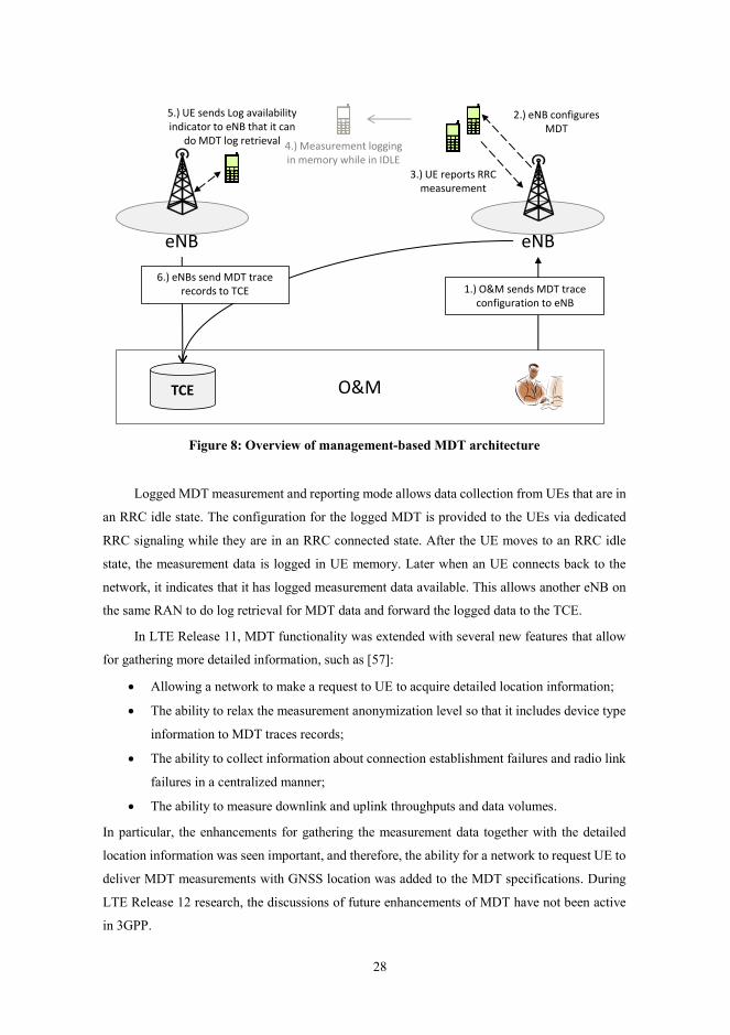
28
Figure 8: Overview of management-based MDT architecture
Logged MDT measurement and reporting mode allows data collection from UEs that are in
an RRC idle state. The configuration for the logged MDT is provided to the UEs via dedicated
RRC signaling while they are in an RRC connected state. After the UE moves to an RRC idle
state, the measurement data is logged in UE memory. Later when an UE connects back to the
network, it indicates that it has logged measurement data available. This allows another eNB on
the same RAN to do log retrieval for MDT data and forward the logged data to the TCE.
In LTE Release 11, MDT functionality was extended with several new features that allow
for gathering more detailed information, such as [57]:
Allowing a network to make a request to UE to acquire detailed location information;
The ability to relax the measurement anonymization level so that it includes device type
information to MDT traces records;
The ability to collect information about connection establishment failures and radio link
failures in a centralized manner;
The ability to measure downlink and uplink throughputs and data volumes.
In particular, the enhancements for gathering the measurement data together with the detailed
location information was seen important, and therefore, the ability for a network to request UE to
deliver MDT measurements with GNSS location was added to the MDT specifications. During
LTE Release 12 research, the discussions of future enhancements of MDT have not been active
in 3GPP.
eNB eNB
TCE
3.) UE reports RRC measurement
2.) eNB configures MDT
5.) UE sends Log availability indicator to eNB that it can
do MDT log retrieval
1.) O&M sends MDT trace configuration to eNB
4.) Measurement logging in memory while in IDLE
O&M
6.) eNBs send MDT trace records to TCE

29
3.2.3 MDT Measurements
The MDT procedure allows operators to collect radio measurements, i.e. received signal strength
and quality, with UE location information and a time stamp. In immediate MDT, the
measurements can be conducted either periodically or when a trigger such as a network event
happens [44]. In logged MDT, the measurements are collected periodically. The MDT
measurements consist of:
The location information with the longitude and latitude (if available);
A time stamp either from a UE or eNB depending on the MDT mode;
The cell identification data and the radio measurements for serving cell and detected intra-
frequency, inter-frequency and inter-RAT neighboring cells.
There are different mechanisms for estimating user location. The most coarse location info is the
serving Cell Global Identification (CGI) and in the best case detailed location information is
obtained from the Global Navigation Satellite System (GNSS). If detailed location information is
obtained from GNSS, then the measurement report shall consist of latitude and longitude, and a
GNSS time stamp. Depending on availability, altitude, uncertainty and confidence can be also
included [44]. It is worth noting that for immediate MDT, the network can make a UE attempt to
make GNSS location information available for MDT [44].
With immediate MDT, the UE does not send time stamp information as it does in the case
of logged MDT. Instead the eNB is responsible for adding the time stamp to the received MDT
measurement reports when saving them to the trace records. However, if GNSS was used, the
GNSS time information is included as a way to validate the detailed location information [44]. It
is anticipated that this will allow outdoor samples to be separated from MDT samples where
location is not known. The cell identification information consists of the serving cell CGI or
Physical Cell Identifications (PCI) of the detected neighboring cells. The measurements for both
the serving and neighboring cells include the Reference Signal Received Power (RSRP) and
Reference Signal Received Quality (RSRQ) for LTE. Similarly, common pilot channel Received
Signal Code Power (RSCP) and received signal quality (EC/N0) are measured for a UTRAN
system [44].
The MDT procedure can also be used to obtain a UE location for UE accessibility failure
reports, for enhanced radio link failure reports, and for other network measurements that are
conducted in RAN nodes [44]. The RAN node measurements are used for QoS verification that
consists of for example, IP throughput and data volume measurement that can be conducted
separately for both a downlink and uplink direction per QCI or per UE in an eNB [44]. The
accessibility measurement refers to the logging details of the failed RRC connection
establishment attempts and reporting the logs to the network after a successful connection

30
establishment [44]. Similarly, RLF reporting refers to the logging information of the connection
failures experienced by the UE [59]. The connection failure can be a radio link or a handover
failure which is triggered if the signal quality in the serving cell reaches an intolerable level, if a
random access procedure fails or if the maximum number of Radio Link Control (RLC)
retransmissions are sent [58]. Since the content of the accessibility and RLF reports can be similar
to the MDT reports, they can be combined and correlated to obtain a comprehensive view of
network coverage, capacity and quality.
It is expected that the MDT measurement procedure allows operators to gather huge
amounts of field measurement data. However, this can easily overcrowd operator databases, and
therefore, cost efficient and agile methods for processing the databases are needed in order to
acquire information and knowledge from the data. Two essential problems with big databases
are information overflow and the “curse of dimensionality”. These problems must be addressed
while analyzing and transforming raw measurements into meaningful information. Information
overflow refers to a problem where the number of data samples is too big to be processed
manually in a way that data analysis can provide useful knowledge. For example, in the case of
network alarm floods, some alarms are ignored because it would be too time consuming to process
them all. The curse of dimensionality refers to a problem where the dimensions of data samples
are high and this makes accurate and efficient processing of such data cumbersome. Methods for
addressing these problems are discussed in Chapter 4 and the applications where knowledge
mining can be used to process the MDT databases are discussed in Chapter 5.
31
4. Means and Methods for Supporting Network Self-
Organization
his chapter introduces the fundamental principles of knowledge mining and control theory
that can provide means and methods for designing automated solutions that address the
challenges of network self-organization. Some alternative theories for design principles can be
found for example in [60].
4.1 Autonomic Control Function
In automation and control theory, the main principle is that control functions adjust a target
system, i.e. network elements, based on references and a feedback loop in order to achieve the
desired behavior [61]. This process is illustrated in Figure 9. By using incremental steps and a
feedback loop, a control function can autonomously react to changes in the output of a target
system. The changes can be normal due to the dynamic nature of the target system or they can be
unexpected due to disturbance, uncertainty and noise. It is anticipated that the deployment of a
reliable and robust self-organizing network requires intelligent control functions that can tolerate
higher degrees of disturbance, uncertainty and noise as a result of the complexity of radio
networks which was discussed in Chapter 3. Automation of such networks is challenging because:
A desired system output can be achieved by tuning many different system parameters,
but since control parameters can have intricate interdependencies, there is uncertainty
with regards to how the chosen parameter combination affects overall system
performance.
Different SON functions that control one network element can have conflicting goals and
this requires coordination between the SON functions to ensure robust behavior.
However, coordination can limit control function behavior, thus resulting in suboptimal
behavior and disturbance.
Neighboring network elements also have complex dependencies. Hence, the control
decisions in one network element can cause noise and disturbances in the desired behavior
of the SON functions in its neighboring elements. Thus, coordination is also required
between the SON functions inside one network element as well as between its nearest
neighbors.
T
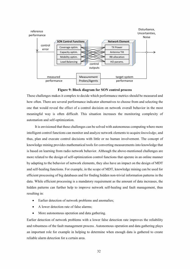
32
Figure 9: Block diagram for SON control process
These challenges makes it complex to decide which performance metrics should be measured and
how often. There are several performance indicator alternatives to choose from and selecting the
one that would reveal the effect of a control decision on network overall behavior in the most
meaningful way is often difficult. This situation increases the monitoring complexity of
automation and self-optimization.
It is envisioned that these challenges can be solved with autonomous computing where more
intelligent control functions can monitor and analyze network elements to acquire knowledge, and
thus, plan and execute control decisions with little or no human involvement. The concept of
knowledge mining provides mathematical tools for converting measurements into knowledge that
is based on learning from radio network behavior. Although the above-mentioned challenges are
more related to the design of self-optimization control functions that operate in an online manner
by adapting to the behavior of network elements, they also have an impact on the design of MDT
and self-healing functions. For example, in the scope of MDT, knowledge mining can be used for
efficient processing of big databases and for finding hidden non-trivial information patterns in the
data. While efficient processing is a mandatory requirement as the amount of data increases, the
hidden patterns can further help to improve network self-healing and fault management, thus
resulting in:
Earlier detection of network problems and anomalies;
A lower detection rate of false alarms;
More autonomous operation and data gathering.
Earlier detection of network problems with a lower false detection rate improves the reliability
and robustness of the fault management process. Autonomous operation and data gathering plays
an important role for example in helping to determine when enough data is gathered to create
reliable alarm detection for a certain area.
Measurement Probes/Agents
reference performance
controloutputs
measured performance
target systemperformance
Disturbance,Uncertainties,
Noise
controlerror
Coverage optim.
Capacity optim.
Mobility optim.
Load Balancing
TX Power
Antenna Tilt
RB allocation
HO params.
SON Control Functions Network Element

33
4.2 Principles of Knowledge Mining
Knowledge mining is a concept that is used for extracting interesting, previously unknown and
potentially useful information from a large amount of data [62]. The process of knowledge mining
usually consists of several phases such as data cleaning, database integration, relevant data
selection, data mining, and data pattern evaluation. Data cleaning, integration and selection are
preprocessing phases where data is prepared for further analysis. Knowledge mining itself can
consist of several different functionalities such as classification; clustering and association of
data; dimensionality reduction and outlier detection to name a few [62]. In the pattern evaluation
phase, information patterns are visualized and analyzed to see if novel and valid information can
be extracted. It is worth highlighting that even if interesting information patterns are discovered,
it does not mean that it is automatically usable or useful. Therefore, information patterns need to
be validated. The following subsections describe in more detail the data mining methods that were
used in [P1-P8].
4.2.1 Classification
Classification refers to a supervised learning process for determining a set of models that describe
data classes. The purpose of using these models is to classify new data which class is unknown
[62]. Sometimes classification is also used to determine missing values in new data by finding the
best matching class which characteristics are used for predicting the missing values. The models
for describing the classes can be presented in many ways. Often models such as decision trees,
statistical models or mathematical models are used. For example, classification algorithms such
as rough sets and classification and regression trees (CART), were used for performance
measurement analysis in GSM networks in [63].
In this thesis, the decision tree-based approach was used in [P2] to classify radio link failures
to coverage failures, interference failures and handover failures. The tree was deduced based on
expert knowledge rather than by means of autonomous machine learning. In addition, a
mathematical model of k-Nearest Neighbors (KNN) was used in [P5] to find similarities between
labeled and unlabeled MDT measurements. A similar approach in principle was also applied in
[P6] and [P7] for RF fingerprint positioning of MDT samples. The k-Nearest Neighbors
classification consists of two steps as described in [62]. First, a set of data samples where the class
label is known, i.e. training samples, are used to construct an n-dimensional training database. In
the second step, all data samples where the class label is unknown, i.e. testing samples, are labeled
by finding the k nearest training samples among all samples in the training data base. The
complexity of the KNN depends on the number of samples in both the training and testing sets,
as well as on the dimensionality of the data samples. The algorithm searches for the nearest
neighbors because typically a distance metric is used to determine the similarity of the samples.

34
Various distance metrics for determining the nearest neighbors can be used. In [P5], the
well-known Euclidean distance de between training sample p and the testing sample q was used
and it is given as,
, ,T
ed p q q p q p (4.1)
where p and q are the k-dimensional column vectors in the embedded space that correspond to
the diffusion distance between the p and q in high dimensional space. In [P6] and [P7],
Mahalanobis distance and Kullback-Leibler Divergence (KLD) were employed to determine the
nearest neighbors. Mahalanobis distance dm is given as,
1, ,T
md pp q q p Σ q p (4.2)
where (.)T denotes the transpose operation and (.)-1 denotes the matrix inverse. In (4.2), the
distance is normalized based on the inverse of the covariance matrix Σp to make it scale-invariant.
Kullback-Leibler Divergence dkl is a non-symmetric measure of the relative entropy between two
probability distributions rather than distance and it is given as,
1 1 11, , ln ,
2
T
kl p q p q pd tr Σ Σ Σ I Σq p Σp q q p (4.3)
where tr(.) denotes the trace operation, |.| is the determinant operation and I is the identity matrix.
One notable difference between dm and dkl is that in (4.3), the covariance matrix Σq and inverse
of the covariance matrix Σp are used whereas in (4.2) only the inverse of the covariance matrix of
training data p is employed. The final step in the KNN algorithm is to label the unknown sample
based on the k nearest training samples. There are various ways to define the class based on the
characteristics of nearest neighbors. One simple way for example, is to use the most common
class among the k nearest training samples.
4.2.2 Clustering
Clustering refers to an unsupervised learning process where data is grouped into different clusters,
i.e. classes without predefined labels, by maximizing the similarities among the samples within
one cluster while minimizing the similarities with samples in other clusters [62]. In clustering, the
purpose is to find methods for measuring similarity or dissimilarity between the samples in
different clusters. For numerical variables, distance metrics such Euclidean distance, as in (4.1),
can be used. For other variable types such as categorical data or a mixture of numerical and
categorical data, more sophisticated similarity metrics are needed. For example, if data contains
categorical values such as a type of failure, it is not self-evident how one can measure the
dissimilarity between the different failure types. Moreover, in some applications, numerical
variables must be unitless variables, i.e. standardized, to avoid the dependence of the chosen

35
measurement unit [62]. Hence, by standardizing the measurement, one attempts to weigh all of
the different variables in the n-dimensional data set equally. For this purpose (4.2) can be used.
A heuristic method of k-means clustering has been applied in [P4] to find clusters for both
normal and anomalous samples. The k-means algorithm partitions a set of numerical samples into
k clusters where the center of the cluster is defined for example, as the mean value of all samples
belonging to the cluster. In the beginning, randomly selected k samples present k different clusters
and their centers. The remaining samples are assigned to different clusters one by one based on
the distance to the center of the cluster. After finding the cluster with the shortest distance, the
centers of the clusters are updated with new mean values that take the new sample into account.
One of the drawbacks of the k-means clustering algorithm is that it is not suitable for detecting
nonconvex shapes or clusters of very different sizes. In addition, it is sensitive to noise and outliers
because a small number of such points can influence the value of the center of point [62].
4.2.3 Anomaly Detection
Anomaly detection or outlier detection refers to a use case for clustering where the purpose is to
cluster samples into two groups. One group contains samples with consistent behavior and the
other contains samples with inconsistent behavior. This procedure typically consists of two steps.
The first step is to define a criterion for consistent and inconsistent data samples. This requires
expertise and knowledge about the behavior of data. In the second step, an efficient method for
detecting the samples that have similar characteristics as the inconsistent samples is employed.
Several approaches for outlier detection can be found in the literature, for example statistical-
based, distance-based, density-based and deviation-based outlier detection approaches [62], [64].
In the scope of cellular networks, the anomaly detection task could be to find anomalous
network elements, for example eNBs, whose behavior is inconsistent and suspicious.
Traditionally, the detection of suspicious behavior has been based on the network alarms which
trigger when test statistics based on the event counts exceeds a predefined threshold [42]. There
are at least two different fundamental principles for detecting anomalies in base station behavior.
This was discussed in [42], [P5]. The anomalies can be detected:
In time domain by explicit learning;
In the network element domain by correlating.
In time domain detection, the behavior of a target base station is compared with its observed
behavior earlier in time. For this reason, time domain profiles are created. However, anomaly
detection in time domain can be tricky due to the seasonal or other cycling changes, and thus, the
anomalies can be hidden in the trend, thus making detection more challenging [62]. Creating
reliable time domain profiles can require long monitoring and data gathering periods.
36
On the other hand, inconsistencies can be detected in a base station domain by comparing
the behavior of the target base station to the behavior of other similar base stations. The
assumption is that base stations with similar characteristics, for example neighboring base
stations, correlate on some level when they are operating as expected. Therefore, a lack of
correlation would reveal suspicious behavior. In the latter case, more data is gathered in a shorter
time period and long learning periods in time domain are not needed, but the data can be biased
if the neighboring base stations behave differently, for example due to the slightly different
parameterization. In [65], the correlation of the network load levels in neighboring base stations
was studied based on empirical data from a 3G network. The study indicated surprisingly low
correlation levels between the neighboring cells. Only 14% of the neighboring cells had a
correlation that was higher than 0.5 when load statistics were collected with a granularity of one
hour.
In [42], time domain and base station domain detection algorithms were introduced based
on the observations of the loading levels in the base stations. In [43], a hierarchical fault detection
framework for detecting faults in a base station on a sector and a carrier level was introduced. In
the hierarchical detection framework, statistical hypothesis tests are used based on a combination
of parametric and non-parametric test statistics. The difference is that the parametric statistical
test can be used when the test statistics are drawn from known distributions whereas the non-
parametric tests are employed when the distributions are unknown. In [66], [67] and [68], the
anomaly detection is based on the statistical profiling in time domain. In [66], a general detection
and diagnosis framework is introduced. The detection is based on creating statistical profiles of
KPIs which are associated with faults. The framework has similarities with the Case-Based
Reasoning methodology since the fault knowledge database is learned autonomously (or with
expert assistance) from earlier fault situations. In [67], detection is improved by learning statistical
profiles by constructing empirical distributions rather than by using normally distributed KPI
statistics as in [66]. The improved detector is based on a common statistical primitive derived
from the sample Kolmogorov-Smirnov test and its performance is validated by analyzing the
amount of voice and data call establishments per cell in live 3G networks. In [68], the detection
is also based on the uplink packets that are used for establishing data connections. However, in
this case, a Kullback-Leibler Diverge metric is used for discriminating between the empirical
distributions. In this thesis, particularly in [P4], [P5], anomaly detection relies on learning but the
statistical apparatus and the test statistics are different.
The anomaly detection in [P4] is done jointly based on the distance and the density metrics
of the test samples in low dimensional embedded space. It was observed that by using both
metrics, anomaly detection is improved compared with a case where only a density metric is
employed. Hence, a sample is an anomaly if it is far away from the group of common samples

37
and it does not have many similar samples nearby that indicate another undiscovered group of
common samples. In [P4], the density of the samples is determined based on the k-dimensional
ball. For each point in the embedded space, a k-ball with a certain radius is defined and the density
is calculated based on the samples which lay inside the ball by using any normalized density
function. Since the scale of each diffusion coordinate in the embedded space is different, the ball
radius is scaled as well. The density ρm of the mth point is defined as,
1
,mm M
ii
(4.4)
where ηm is the number of points inside the ball and the sum in the denominator is norm-1 over
all M points. If the density of a certain point is large in the embedded space then it has many
neighbors nearby and it is considered to be regular. On the contrary, irregular points would have
a small density. After obtaining the densities, k-means clustering was employed to search for the
anomalous samples. The k-means algorithm used Euclidean distance metric to group the samples
consisting of seven variables in the embedded space. That is, each sample consisted of the six
most meaningful diffusion coordinates and the density variable.
In [P5], the anomaly detection is based on tracking the absolute standard score in the base
station domain. First, a statistical model for network outage behavior for a set of base stations is
constructed based on the observations during the learning phase. Later in the tracking phase, the
absolute standard score, i.e. the anomaly score, for each base station is computed as,
,i L
i
L
xz
(4.5)
where variable xe is the number of outage samples associated with eNB i and variables μL and σL
are the expected mean and standard deviation of the outage samples that characterize outage
behavior in the eNBs local neighborhood during the learning phase. If zi is much larger than one,
then eNB i is expected to be an anomaly since the number of outage observations does not fit
within the normal deviation of the outage observations.
4.2.4 Dimensionality Reduction
The goal of dimensionality reduction is to represent high dimensional data sets in a lower
dimensional space in order to reduce the computational complexity of knowledge mining and to
address the curse of dimensionality. The curse of dimensionality refers to various problems in
classification, clustering and anomaly detection. Typically, using fewer variables or features in
knowledge mining makes the mining process faster, less complicated and more robust. Widely
used dimensionality reduction methods are for example, an attribute selection method and a data
compression method. In attribute selection, one tries to select a minimum subset of attributes so

38
that the data mining result will be as close as possible to the result that would be obtained by using
the all attributes [62]. The best attributes can be selected for example, based on expert knowledge
or statistical significance, assuming that the attributes are independent from each other [62]. In
data compression, encoding or transformations are used to obtain a compressed representation of
data [62]. Principal Component Analysis (PCA) is a widely used linear data compression method
where k most significant orthonormal vectors are used to project n-dimensional data onto a lower
k-dimensional subspace while still providing a good approximation of the original data in the
lower subspace.
In [P4] and [P5], a non-linear data compression method known as Diffusion Maps is used.
Diffusion Maps is a dimensionality reduction method for finding meaningful geometrical
descriptions of the high dimensional data sets. It is done by constructing diffusion coordinates
and diffusion distance metrics that parameterize the original data set and provide a local
preserving metric for the data [69], [70], [71], [72]. Parameterization is done by using a graph G
and a weight function kernel W that measure the pairwise similarity of the points in a training set.
If a proper kernel function is used, then W can be normalized into a Markov transition matrix.
The diffusion is created by conducting a random walk to this transition matrix. The most
significant eigenfunctions, i.e. the functions associated with largest eigenvalues, of the transition
matrix provide a good low dimensional geometric embedding of the data in a way that Euclidean
distance in the embedding space measures the meaningful diffusion metrics of the data. The
expression of the diffusion distance Dt2(.) between data points xi and xj can be given as in [72],
2
2 2
j
1
( , ) ,k
t
t i l l i l j
l
D x x x x
(4.6)
where k is the number of the most significant eigenvectors, t represents the depth of the random
walk and variable λl is the eigenvalue of the lth eigenvector. The variables ψl(xi) and ψl(xj) are the
lth entries of the right eigenvectors of the transition matrix for points xi and xj. Moreover, the
diffusion coordinates are constructed using k most significant right eigenvectors and eigenvalues
as described in [72],
1( ) ( ),..., ( ) ,t t
t i i k ix x x (4.7)
where the diffusion coordinates for ith data sample xi can be obtained from m-by-k diffusion
coordinate matrix Ψt. The column vectors of Ψt are the right eigenvectors of Markov transition
matrix multiplied by the corresponding eigenvalue term λk as shown in (4.7). Moreover, the
diffusion coordinates for a particular point xi are found in the ith row vector of the diffusion
coordinate matrix Ψt. As seen from (4.6) and (4.7), the diffusion distance for samples in the high
dimensional space corresponds to the Euclidean distance of the samples in the embedded space.

39
5. Knowledge Mining Assisted Network
Performance Improvements
his chapter walks readers through various knowledge mining assisted methods that improve
the performance of cellular network. The motivation for using these methods comes from
the fact that networks are getting denser and more complex, thus requiring efficient new ways to
operate a network.
5.1 Coverage Optimization with Extended RLF Reports
As described in Section 3.2.3, RLF reporting provides a mechanism for a UE to indicate that it
has encountered a connection failure. This is a strong indicator from a UE that something is
wrong. By extending the RLF report to contain additional information, for example location, radio
measurements and cell identification data, it becomes easier to analyze the root cause of the RLFs
and learn how networks should be optimized to avoid the occurrence of similar problems. For this
reason, coverage optimization of an irregular network layout was studied in [P2] with the
assistance of extended RLF reports. It was anticipated that the irregular network layout provides
a realistic simulation environment for studying coverage hole related problems due to diverse
coverage and interference conditions [P1]. In addition to irregular topology, four artificial
coverage holes with a radius of 180 meters were modeled in a system simulator to further
emphasize the heterogeneity of the studied scenario. The coverage holes were placed in four
different locations: two at the intersection of the border area of three sites with short and long
inter-site distance; one between two sites and one at the center of a single sector. It is worth
pointing out that the coverage and the interference conditions are quite different depending on the
location of the coverage holes.
Coverage optimization was carried out by constructing a classification tree for
discriminating between different types of RLFs. The structure of the classification tree was
derived from the radio measurements and the number of identified cells reported along with the
RLF reports. The structure of the classification tree is illustrated in Figure 10. It is expected that
RLF is caused by a coverage problem if only the serving cell is identified and the RSRP threshold
is below a predefined level of -120 dBm. If RSRP is above the threshold level, an interference
problem is assumed be the cause of the problem. This is the case because downlink RSRP is
acceptable, but no other neighbors are detected. If the UE can identify several neighbor cells in
addition of the serving cell, the root cause of RLF can be classified as either a coverage problem
or a mobility problem. Mobility problems are expected to occur due to the poor selection of
T

40
handover parameters or missing neighbor relations. In this study, RLF is classified as a mobility
problem if an A3 event has been sent or if the RSRP difference between target cell and serving
cell is negative prior to RLF. A negative RSRP difference indicates that the signal level in one of
the neighbor cells is stronger compared to the serving cell.
Therefore, the neighboring cell is a better candidate for being a new serving cell and it is
likely that a handover to this cell should have been done earlier. The classification and simulation
results presented in [P2] suggest that the severity of the coverage problems depend on the location
of the coverage hole whereas interference and mobility problems were caused mainly by network
loading and handover parameterization. If larger offsets or longer time-to-trigger values are
configured then the number of mobility related RLFs increase even if no artificial coverage hole
exists. Specifically, Figure 6 in [P2] shows that the number of mobility related RLFs increase
even in low loaded network if UE velocity is 30 km/h. However, the increase is relatively smaller
compared with the RLFs that are observed with higher network loadings. It was concluded that
classification of the extended RLF reports provides additional value to the MDT coverage
optimization use case, since it can provide a better understanding of the root cause of RLFs with
a rather low false alarm rate. It is worth highlighting that the tree was not constructed
autonomously in this study. Instead, expert knowledge was used to develop the structure of the
tree. Hence, it would have been interesting see the shape of the tree if machine learning would
have been used.
Figure 10: Classification tree for RLF problems
RLF Report
IdentifiedCells?
RSRP?
1
A3?
>= 2
Coverageproblem
Interferenceproblem
<= threshold > threshold Sent
Mobilityproblem
Not sent
RSRP Difference
?
Coverageproblem
Mobilityproblem
>= 0 dB < 0 dB
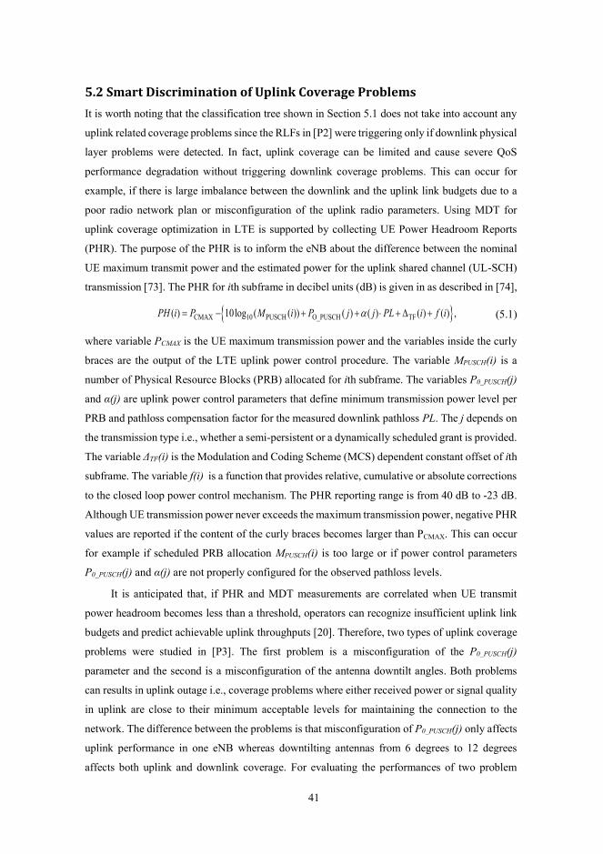
41
5.2 Smart Discrimination of Uplink Coverage Problems
It is worth noting that the classification tree shown in Section 5.1 does not take into account any
uplink related coverage problems since the RLFs in [P2] were triggering only if downlink physical
layer problems were detected. In fact, uplink coverage can be limited and cause severe QoS
performance degradation without triggering downlink coverage problems. This can occur for
example, if there is large imbalance between the downlink and the uplink link budgets due to a
poor radio network plan or misconfiguration of the uplink radio parameters. Using MDT for
uplink coverage optimization in LTE is supported by collecting UE Power Headroom Reports
(PHR). The purpose of the PHR is to inform the eNB about the difference between the nominal
UE maximum transmit power and the estimated power for the uplink shared channel (UL-SCH)
transmission [73]. The PHR for ith subframe in decibel units (dB) is given in as described in [74],
CMAX 10 PUSCH O_PUSCH TF( ) 10log ( ( )) ( ) ( ) ( ) ( ) ,PH i P M i P j j PL i f i (5.1)
where variable PCMAX is the UE maximum transmission power and the variables inside the curly
braces are the output of the LTE uplink power control procedure. The variable MPUSCH(i) is a
number of Physical Resource Blocks (PRB) allocated for ith subframe. The variables P0_PUSCH(j)
and α(j) are uplink power control parameters that define minimum transmission power level per
PRB and pathloss compensation factor for the measured downlink pathloss PL. The j depends on
the transmission type i.e., whether a semi-persistent or a dynamically scheduled grant is provided.
The variable ΔTF(i) is the Modulation and Coding Scheme (MCS) dependent constant offset of ith
subframe. The variable f(i) is a function that provides relative, cumulative or absolute corrections
to the closed loop power control mechanism. The PHR reporting range is from 40 dB to -23 dB.
Although UE transmission power never exceeds the maximum transmission power, negative PHR
values are reported if the content of the curly braces becomes larger than PCMAX. This can occur
for example if scheduled PRB allocation MPUSCH(i) is too large or if power control parameters
P0_PUSCH(j) and α(j) are not properly configured for the observed pathloss levels.
It is anticipated that, if PHR and MDT measurements are correlated when UE transmit
power headroom becomes less than a threshold, operators can recognize insufficient uplink link
budgets and predict achievable uplink throughputs [20]. Therefore, two types of uplink coverage
problems were studied in [P3]. The first problem is a misconfiguration of the P0_PUSCH(j)
parameter and the second is a misconfiguration of the antenna downtilt angles. Both problems
can results in uplink outage i.e., coverage problems where either received power or signal quality
in uplink are close to their minimum acceptable levels for maintaining the connection to the
network. The difference between the problems is that misconfiguration of P0_PUSCH(j) only affects
uplink performance in one eNB whereas downtilting antennas from 6 degrees to 12 degrees
affects both uplink and downlink coverage. For evaluating the performances of two problem

42
scenarios, statistics for PHR, UL received power and UL signal to interference ratio were
compared with the performance of the optimized reference scenario. In the reference scenario, the
uplink power control parameters were configured according to a strategy where a scheduler aims
to schedule one PRB UL-SCH allocation for UEs at the cell edge as discussed for example in
[38]. This ensures that the UEs will allocate all available power to the single PRB at the cell edge,
thus maximizing the received power per Hz and the uplink coverage. By adjusting the uplink
power control parameters, more bandwidth at the cell edge can be provided. However, if
P0_PUSCH(j) is reduced too much in contrast to the chosen α(j), then uplink transmission may drown
out in the noise, thus resulting in uplink coverage problems that cannot be not detected by
observing PHR.
Table I and II gather the main results from the figures presented in [P3] and show the
performance comparison between the studied scenarios for the three centermost base stations.
These base stations are eNB-8, eNB-16 and eNB-18. In Table I, the performance indicators are
for the simulated scenarios where a parameter for building penetration loss was set to 10 dB. The
values in Table II correspond to the simulations where the building penetration loss was increased
to 15 dB. The following conclusion was made based on the simulation results in [P3]. First of all,
PHR behavior depends on the uplink power control parameterization and the scheduled allocation
size. If one is confident that uplink coverage problems are not caused by misconfiguration of the
power control parameters, then PHR condition exceeding a threshold can be used to detect uplink
problems. This can be seen by observing the probability of PHR being less than 0 dB, thus
meaning that all available power is used. In the coverage problem case that is caused by overtilted
antennas, the probability of PHR exceeding the threshold is much higher than in the reference
case. However, it is beneficial to scale the PHR with the allocation size before making any
conclusion about uplink coverage problems in order to avoid unnecessary signaling over the air
interface. It was observed in [75], that the probability of PHR exceeding the threshold is
approximately 35% if PHR is not scaled whereas for the scaled PHR the corresponding
probability was around 5%, thus indicating significantly less false alarms.
It was also observed that if the power control parameters are not configured properly, PHR
do not necessarily trigger at all. This can be seen by comparing the probability of PHR being less
than 0 dB in the reference and the misconfigured P0_PUSCH(j) scenarios. By reducing the
P0_PUSCH(j), UEs would allocate less transmission power per PRB. This on the other hand results
in larger PHR values which suggest that UE can support larger bandwidth allocations. In this case,
PHR_perPRB do not exceed the threshold but the uplink received power (RXP) and the signal to
interference and noise ratio (SINR) would be very poor, thus suggesting a severe uplink outage
as show in Table I and Table II.

43
Table I: Uplink performance indicators for 10 dB building penetration loss scenarios [P3]
Building Penetration
Loss is 10 dB
Reference Misconfigured P0 Overtilted antennas
eNB-8 eNB-16 eNB-18 eNB-8 eNB-16 eNB-18 eNB-8 eNB-16 eNB-18
Pr( PHR_perPRB < 0dB ) 5.0% 2.5% 5.0% 0.0% 3.1% 4.0% 20.0% 13.0% 9.0%
5%-ile UL SINR [dB] -1.8 -1.3 -2.1 -14.2 -1.1 0 -3.5 -1.8 -1.8
5%-ile UL RXP [dBm] -114 -113 -114 -124 -113 -114 -119 -116 -116
Table II: Uplink performance indicators for 15 dB building penetration loss scenarios [P3]
Building Penetration
Loss is 15 dB
Reference Misconfigured P0_PUSCH(j) Overtilted antennas
eNB-8 eNB-16 eNB-18 eNB-8 eNB-16 eNB-18 eNB-8 eNB-16 eNB-18
Pr( PHR_perPRB < 0dB ) 4.0% 1.9% 3.5% 0.0% 1.4% 3.8% 14.0% 8.2% 9.0%
5%-ile UL SINR [dB] -3.8 -3.6 -3.6 -16.1 -3.7 -3.5 -5.9 -4.5 -4.2
5%-ile UL RXP [dBm] -120 -119 -120 -130 -119 -120 -124 -122 -123
According to the link level simulation results and a link budget calculation, SINR and RXP
threshold values of -5 dB and -123 dBm are reasonable values for the uplink outage. The dotted
horizontal lines in [P3] resembles these thresholds. According to Table I and Table II, these
threshold are not exceeded at the cell edge in the reference case. However, in case of the parameter
misconfiguration, the thresholds are exceeded indicating uplink outage.
5.3 MDT assisted Sleeping Cell Detection
The purpose of self-healing is to provide functions which improve automatic control of cellular
network operations for detecting and handling network failures. A sleeping cell is a special case
of malfunctioning base station where the base station appears to be operable while its performance
is degraded. One approach for detecting a sleeping cell is to monitor the changes in the base
station’s neighbor relation patterns as suggested in [76]. Another approach is to monitor network
traffic and loading profiles and detect suspicious behavior from these profiles as discussed in [42],
[65]. In [P4] and [P5], the goal is to study an alternative framework for detecting a sleeping cell
with degraded downlink performance. The detection framework is based on employing the
Diffusion Maps knowledge mining method to find hidden patterns from MDT databases. The
research was carried out by conducting system simulations for gathering MDT reports and RLF
reports. In the reference scenario, the network is in healthy state, coverage is optimized, and the
RLF rate is low. In the problem scenario, the antenna line for eNB-8 is malfunctioning causing
outage and higher RLF rates. Dominance areas for the reference and the problem scenario in [P5]
are depicted in Figure 11. The dominance area indicates the area where a particular cell is the
strongest serving cell. In the leftmost illustration in Figure 11, the dominance area of eNB-8 is
shown with a turquoise color that covers less than 5% of the analyzed area. This is similar to the
dominance areas of the other cells.

44
a) Optimized reference scenario b) Sleeping cell scenario
Figure 11: Simulated network dominance areas
In the rightmost illustration, eNB-8 is sleeping and it is not transmitting anything in a
downlink direction. Therefore, the area is served by the neighboring cells. It is worth pointing out
that detection of the sleeping cells based only on the RLF reports is not a straight-forward process
for two reasons:
Firstly, the neighbor base stations can partly cover the service area of the sleeping cell.
Thus, the coverage can be weak but severe outage is not necessarily detected.
Secondly, in multi-layer and multi-RAT radio networks, UEs can be handed over to
overlapping layers on a different RAT before RLF triggers.
Hence, the number of RLFs can remain small and detection of outage or sleeping cells based only
on the extended RLF reports become challenging. The motivation for finding hidden patterns
from MDT databases was to identify periodical MDT reports that have similarities with RLF
reports. This is anticipated to enable earlier outage detection even in a case where only an
insufficient amount of RLF reports are observed.
5.3.1 Clustering based approach for Sleeping Cell Detection
In [P4], the purpose is to study how unsupervised k-means clustering method groups extended
RLF reports and those MDT reports that are triggered by an A22 event. Clustering is done for the
reports after transforming them into a low dimensional embedded space by using diffusion maps.
The analyzed MDT and RLF reports contained RSRP and RSRQ radio measurements from the
serving cell and the three strongest neighboring cells on the same frequency band. In addition, it
2A2 Event triggers when serving cell is less than a threshold.

45
is assumed that the eNB would incorporate the Wideband Channel Quality Indictor (WCQI) into
the MDT and RLF reports. Thus, the high dimensional presentation of the MDT and RLF samples
consisted of 9 numerical variables. The MDT reports from the reference simulation are used for
training the Diffusion Maps algorithm to construct the presentation of the embedded space in a
case where the network behavior is normal. After the training phase, all MDT and RLF reports
from the problem scenario were transformed into this embedded space and the samples were
clustered into two groups. The group with most of the sample is assumed to represent the normal
group because it has similar behavior as the MDT reports in the reference simulation. The other
group, the anomalous group, would contain the samples which are not similar to the samples in
the normal group. It is expected that most of the RLFs and some of the A2 events which have
similar characteristics with RLFs would fall into the anomalous group.
After clustering the samples, sleeping cell detection is done by finding the most probable
dominance area for the anomalous samples by comparing their location, i.e. by using GNSS
coordinates or RF fingerprint, with the operator’s database of the dominance areas. This is
illustrated in Figure 12. In this study, the availability of GNSS coordinates is assumed to be ideal,
and therefore, the correlation between the location of the anomalies and the expected dominance
areas was simple. The performance results indicated that the majority of the anomalies, i.e. more
than 50%, fall into the dominance areas of eNB-8 and eNB-16 as illustrated in Figure 12. eNB-8
is the sleeping cell and eNB-16 is an adjacent cell to the sleeping cell. In addition, it was observed
that approximately one-third of the anomalies associated with eNB-8 were MDT reports triggered
by an A2 event, thus suggesting that sleeping cell detection would be possible to some extent
based solely on the MDT reports without knowledge of RLFs.
Figure 12: Number of anomalies per e-NB
eNB ID
Nu
mb
er
of
ano
mal
ies

46
It is worth highlighting that MDT reports with less accurate location information increase
the probability of associating anomalies with the dominance area of wrong base station.
According to the simulation results in [P7], two-thirds of MDT reports can be located with
positioning error less than 276 meters if fingerprinting is used. However, if one of the cells is
sleeping, the error of fingerprinting can be even more significant. It is expected that in such case
the anomalous measurements are distributed among neighboring base stations. This increase the
amount of MDT measurements that are needed to detect the problem. On the other hand, network
can control which MDT samples are used to detect the anomalies. If enough measurements can
be obtained with accurate location information then samples with less accurate location can be
neglected.
5.3.2 Classification based Approach for Sleeping Cell Detection
In [P5], sleeping cell detection was improved by classifying all periodical MDT reports and
extended RLF reports into three classes: Periodical, Handover and Outage. This was done by
using the KNN classification algorithm based on the diffusion coordinates and distance. The
motivation for classifying the periodically transmitted MDT reports is to detect areas which have
similarities with the samples that belong to the outage category. This is different from [P4], where
clustering is employed only for MDT reports that are triggered by an A2 event condition. The
performance of the classification is verified by using 8-feature and 10-feature classifiers. The 8-
feature classifier analyzes MDT and RLF reports that contain only RSRP and RSRQ radio
measurements from the serving cell and the three strongest neighboring cells whereas the 10-
feature classifier assumes that the serving eNB would include two additional measurements
(WCQI and PHR) in the MDT and RLF reports before transmitting the trace records to the TCE
for post processing.
The confusion matrices shown in Table III and Table IV illustrate the classification accuracy
of the 8-feature and the 10-feature classifiers. The diagonal cells of the confusion matrices show
the outcome of a true-positive test which indicates the likelihood that a sample is correctly labeled
according to the class it belongs to. A false-positive test indicates the likelihood that samples are
labeled incorrectly and have been assigned to the wrong classes. Table III shows the classification
accuracy of MDT and RLF samples in the reference simulation. It can be seen that the true-
positive probability is more than 80% for all class types regardless of the classifier that is used.
The 10-feature classifier performs better but the performance of the 8-feature classifier is not
much worse either. It is worth highlighting that we do not expect to achieve 100% classification
accuracy, since it is quite likely that some of the periodical, handover and radio link failures would
have similar characteristics in any case; this is especially true because the periodical reports are
transmitted frequently. The reports preceding a handover or a radio link failure event are assumed

47
to have similar characteristics. The numerical value in parenthesis following the real class label
in the tables indicates the total amount of analyzed samples in each class. After classifying the
MDT reports based on either 8-feature or 10-feature classifiers, the detection of the sleeping cell
is done by counting the number of suspicious MDT reports that have similar characteristics with
samples collected from outage regions i.e., RLF samples. These samples are associated with eNBs
based on the geographical location of the samples and the dominance areas of the eNBs. The
relative number of outage samples that are associated with different eNBs in a case where a 10-
feature classifier is used is shown in Figure 13.
Table III. Confusion matrices for reference simulation data
Real Class 8 features (only RSRP & RSRQ) 10 features (with CQI & PHR)
Per. HO RLF Per. HO RLF
Periodical (148723) 96.4 % 2.9 % 0.7 % 96.6 % 2.9 % 0.5 %
Handover (698) 11.9 % 82.1 % 6.0 % 11.8 % 83.0 % 5.2 %
Radio Link Failure (138) 0.0 % 0.0 % 100 % 0.0 % 0.0 % 100 %
Table IV. Confusion matrices for problem simulation data
Real Class 8 features (only RSRP & RSRQ) 10 features (with CQI & PHR)
Per. HO RLF Per. HO RLF
Periodical (148693) 96.0 % 2.9 % 1.1 % 96.2 % 2.9 % 0.9 %
Handover (683) 13.3 % 79.9 % 6.8 % 12.7 % 81.4 % 5.9 %
Radio Link Failure (210) 3.3 % 0.5 % 96.2 % 1.0 % 1.0 % 98.0 %
a.) Reference scenario

48
b.) Problem scenario
Figure 13: Relative number of different outage samples
Figure 13 shows that in the problem scenario, the increase in the number of outage samples
is significantly larger for eNB-8. Almost 40% of all RLF labeled samples were associated with
the eNB-8 dominance area whereas it was only 3% in the reference scenario. In addition, it was
observed that a large amount of the periodical MDT samples in the dominance area of eNB-8
were classified as outage samples after triggering the problem. This suggests that by finding
similarities between MDT and extended RLF reports:
The detection of outages or weak coverage can be done even in cases where an
insufficient amount of RLF reports are available for a particular area of interest.
In [P5], network alarms trigger if the number of outage samples associated with a particular eNB
is different compared to the behavior of the outage samples in the neighboring eNBs. For
triggering an alarm in eNB i, a base station specific anomaly score zi is used. The figure in [P5]
shows a distribution of the anomaly scores during the reference scenario which indicates that for
the majority of the eNBs, the zi remains below two. Only eNB-6, eNB-18 and e-NB 43 indicated
some outage. However, when the sleeping cell problem is triggered in e-NB 8, the alarm score z8
starts to increase remarkably. Figure 14 illustrates how much data and how long data collection
period is needed to make reliable detection of sleeping cell in a case where the 10-feature classifier
is used. Fast detection requires that enough anomalous data is obtained from UEs moving in the
area of sleeping cell. Hence, the volume of the measurement data depends on the measurement
configuration for collecting the MDT reports, amount of users and users’ mobility patterns. In
Figure 14, the y-axis indicates the anomaly score as shown in (4.5) and the x-axis indicates the
amount of received MDT reports per eNB as the simulation advances in time. The scores are
updated every five seconds using the mean and standard deviation values obtained from the
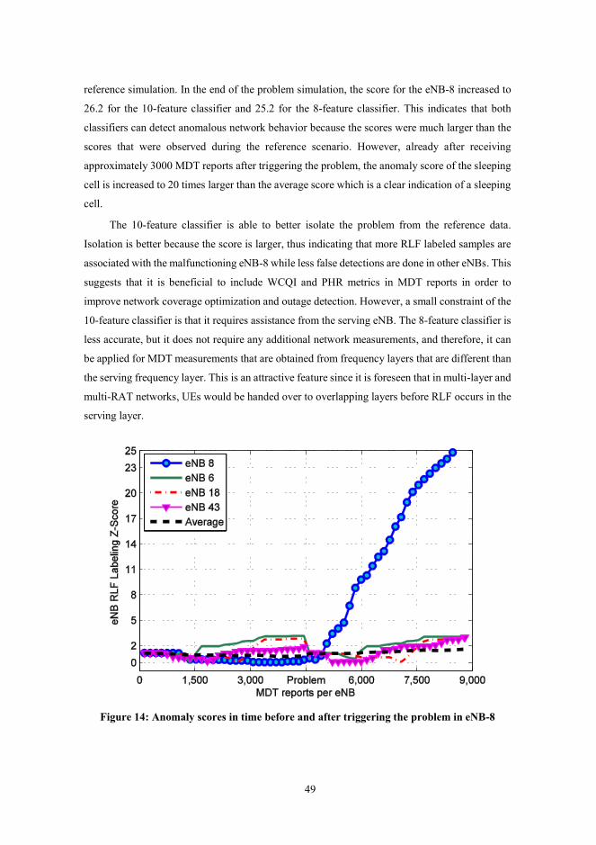
49
reference simulation. In the end of the problem simulation, the score for the eNB-8 increased to
26.2 for the 10-feature classifier and 25.2 for the 8-feature classifier. This indicates that both
classifiers can detect anomalous network behavior because the scores were much larger than the
scores that were observed during the reference scenario. However, already after receiving
approximately 3000 MDT reports after triggering the problem, the anomaly score of the sleeping
cell is increased to 20 times larger than the average score which is a clear indication of a sleeping
cell.
The 10-feature classifier is able to better isolate the problem from the reference data.
Isolation is better because the score is larger, thus indicating that more RLF labeled samples are
associated with the malfunctioning eNB-8 while less false detections are done in other eNBs. This
suggests that it is beneficial to include WCQI and PHR metrics in MDT reports in order to
improve network coverage optimization and outage detection. However, a small constraint of the
10-feature classifier is that it requires assistance from the serving eNB. The 8-feature classifier is
less accurate, but it does not require any additional network measurements, and therefore, it can
be applied for MDT measurements that are obtained from frequency layers that are different than
the serving frequency layer. This is an attractive feature since it is foreseen that in multi-layer and
multi-RAT networks, UEs would be handed over to overlapping layers before RLF occurs in the
serving layer.
Figure 14: Anomaly scores in time before and after triggering the problem in eNB-8

50
5.4 Localization of MDT Radio Measurements
One goal in [P4] and [P5] was to associate the anomalous MDT reports with a base station to
detect sleeping cells based on the geographical location of the anomalous MDT reports and the
dominance areas. As described in Section 3.2, the MDT reports can be located based on the
detailed location obtained from the GNSS receiver or by using RF fingerprinting. If the detailed
location in an MDT report is obtained from the GNSS receiver then the correlation with the
dominance areas is not an issue. However, if one cell is sleeping and it is not detectable, then
positioning based on RF fingerprints can be challenging and can lead to the wrong conclusion
because of missing neighbor measurements.
Typically, RF fingerprinting refers to a database correlation method where the position is
estimated by comparing the radio measurements (the RF fingerprint) of the UEs with the training
fingerprints in the correlation database [77]. The training fingerprints consist of radio
measurements from several base stations that are used to provide a fingerprint of the radio
conditions at a specific geographical location. Typically, this location is determined with an
accurate positioning method, for example GNSS. One of the biggest challenges of RF
fingerprinting is the burden of creating and maintaining the correlation database of the training
fingerprints. Operators can maintain the correlation database by conducting extensive and
expensive periodical drive test campaigns to collect the required measurements. In fact, one of
the benefits of MDT is that it provides an efficient way to automate the collection of training
fingerprints. Hence, the positioning framework for MDT reports that was developed in [P6] and
[P7] is designed to understand how MDT reports can be located based on RF fingerprints in
heterogeneous inter-frequency LTE networks. The framework is developed to study how LTE
network heterogeneity and the number of monitored frequency layers affect RF fingerprint
positioning performance in interference limited LTE deployments. It is anticipated that a
synchronous LTE network is deployed using a frequency reuse 1 strategy, and therefore it is
interference limited. This may restrict the ability of UEs to detect and measure the neighboring
cells that have a negative impact on RF fingerprinting performance.
The RF fingerprinting framework consists of two phases: a training phase and an estimation
phase. In the training phase, a correlation database is created by using MDT reports that contain
detailed GNSS location information. These MDT reports form training fingerprints which are
associated with a search grid that represents the area of interest. In this study, the grid consists of
rectangular grid units of varying size, for example 10-by-10 meters or 40-by-40 meters. This
allows RSRP measurements from different intra- and inter-frequency eNBs to be associated with
different geographical locations. Later in the estimation phase, the locations of the unknown MDT
reports are estimated by searching for a grid unit with the training fingerprint that gives the best
match with the RF fingerprint that is obtained from the unknown MDT reports.
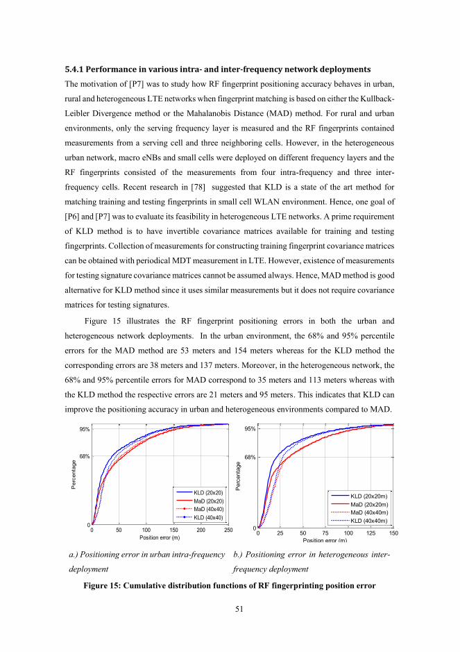
51
5.4.1 Performance in various intra- and inter-frequency network deployments
The motivation of [P7] was to study how RF fingerprint positioning accuracy behaves in urban,
rural and heterogeneous LTE networks when fingerprint matching is based on either the Kullback-
Leibler Divergence method or the Mahalanobis Distance (MAD) method. For rural and urban
environments, only the serving frequency layer is measured and the RF fingerprints contained
measurements from a serving cell and three neighboring cells. However, in the heterogeneous
urban network, macro eNBs and small cells were deployed on different frequency layers and the
RF fingerprints consisted of the measurements from four intra-frequency and three inter-
frequency cells. Recent research in [78] suggested that KLD is a state of the art method for
matching training and testing fingerprints in small cell WLAN environment. Hence, one goal of
[P6] and [P7] was to evaluate its feasibility in heterogeneous LTE networks. A prime requirement
of KLD method is to have invertible covariance matrices available for training and testing
fingerprints. Collection of measurements for constructing training fingerprint covariance matrices
can be obtained with periodical MDT measurement in LTE. However, existence of measurements
for testing signature covariance matrices cannot be assumed always. Hence, MAD method is good
alternative for KLD method since it uses similar measurements but it does not require covariance
matrices for testing signatures.
Figure 15 illustrates the RF fingerprint positioning errors in both the urban and
heterogeneous network deployments. In the urban environment, the 68% and 95% percentile
errors for the MAD method are 53 meters and 154 meters whereas for the KLD method the
corresponding errors are 38 meters and 137 meters. Moreover, in the heterogeneous network, the
68% and 95% percentile errors for MAD correspond to 35 meters and 113 meters whereas with
the KLD method the respective errors are 21 meters and 95 meters. This indicates that KLD can
improve the positioning accuracy in urban and heterogeneous environments compared to MAD.
a.) Positioning error in urban intra-frequency
deployment
b.) Positioning error in heterogeneous inter-
frequency deployment
Figure 15: Cumulative distribution functions of RF fingerprinting position error
0 50 100 150 200 2500
68%
95%
Position error (m)
Perc
enta
ge
KLD (20x20)
MaD (20x20)
MaD (40x40)
KLD (40x40)
0 25 50 75 100 125 1500
68%
95%
Position error (m)
Perc
enta
ge
KLD (20x20m)
MaD (20x20m)
MaD (40x40m)
KLD (40x40m)
51
5.4.1 Performance in various intra- and inter-frequency network deployments
The motivation of [P7] was to study how RF fingerprint positioning accuracy behaves in urban,
rural and heterogeneous LTE networks when fingerprint matching is based on either the Kullback-
Leibler Divergence method or the Mahalanobis Distance (MAD) method. For rural and urban
environments, only the serving frequency layer is measured and the RF fingerprints contained
measurements from a serving cell and three neighboring cells. However, in the heterogeneous
urban network, macro eNBs and small cells were deployed on different frequency layers and the
RF fingerprints consisted of the measurements from four intra-frequency and three inter-
frequency cells. Recent research in [78] suggested that KLD is a state of the art method for
matching training and testing fingerprints in small cell WLAN environment. Hence, one goal of
[P6] and [P7] was to evaluate its feasibility in heterogeneous LTE networks. A prime requirement
of KLD method is to have invertible covariance matrices available for training and testing
fingerprints. Collection of measurements for constructing training fingerprint covariance matrices
can be obtained with periodical MDT measurement in LTE. However, existence of measurements
for testing signature covariance matrices cannot be assumed always. Hence, MAD method is good
alternative for KLD method since it uses similar measurements but it does not require covariance
matrices for testing signatures.
Figure 15 illustrates the RF fingerprint positioning errors in both the urban and
heterogeneous network deployments. In the urban environment, the 68% and 95% percentile
errors for the MAD method are 53 meters and 154 meters whereas for the KLD method the
corresponding errors are 38 meters and 137 meters. Moreover, in the heterogeneous network, the
68% and 95% percentile errors for MAD correspond to 35 meters and 113 meters whereas with
the KLD method the respective errors are 21 meters and 95 meters. This indicates that KLD can
improve the positioning accuracy in urban and heterogeneous environments compared to MAD.
a.) Positioning error in urban intra-frequency
deployment
b.) Positioning error in heterogeneous inter-
frequency deployment
Figure 15: Cumulative distribution functions of RF fingerprinting position error
0 50 100 150 200 2500
68%
95%
Position error (m)P
erc
enta
ge
KLD (20x20)
MaD (20x20)
MaD (40x40)
KLD (40x40)
0 25 50 75 100 125 1500
68%
95%
Position error (m)
Perc
enta
ge
KLD (20x20m)
MaD (20x20m)
MaD (40x40m)
KLD (40x40m)

52
The results in [P7] indicate that the performance of KLD and MAD are similar in rural
deployment. However, in urban and heterogeneous deployments, the KLD method shows better
positioning accuracy compared to the MAD method. It is also noticed that when higher resolution
grids were used, KLD can further improve positioning performance whereas such improvement
is not observed for the MAD method. The performance improvement is highest in the
heterogeneous network. This suggests that by exploiting the interdependencies of the received
signal strengths from different base stations and by incorporating the corresponding covariance
matrices into the RF fingerprints, a promising network-based method for locating MDT reports
can be established.
5.4.2 Performance constraints by 3GPP cell detection performance requirements
In [P7], RF fingerprinting performance was evaluated with the assumption of ideal cell detection
performance; all MDT reports always consisted of measurements from the 4 strongest intra-
frequency and the 3 strongest inter-frequency eNBs regardless of the energy per symbol over
interference plus noise (Ês/Iot) criteria. Such evaluation is a well justified way of comparing the
performance of KLD with the MAD method. However, if ideal cell detection performance is
assumed it can also produce positioning accuracies that are too optimistic. In [P6], the
performance of RF fingerprinting is evaluated by comparing ideal cell detection performance with
the practical cell detection performance. Practical cell detection was taking into account the -6 dB
Ês/Iot criteria from 3GPP specifications [79]. In other words, a cell can only be detected and
measured if Ês/Iot is above -6 dB and RSRP is above -127 dBm.
The performance evaluation is done for the heterogeneous small cell network scenario
(Case0) and the sparse regular macro network scenario (Case4) as show in Figure 16. In both
cases, the deployment is inter-frequency deployment that consists of two layers of eNBs which
operate on adjacent carriers.
a.) Regular macro network b.) Heterogeneous network
Figure 16: Heterogeneous and regular macro network simulation scenarios

53
However, in the regular macro scenario, the sites in the denser frequency layer are deployed in a
coordinated manner whereas in the heterogeneous scenario a random uncoordinated deployment
of small cells is employed. Table V shows the positioning error percentiles for the KLD method,
this is done with and without considering the Ês/Iot criteria. It was observed in [P6] that if Ês/Iot
is taken into account, then the average number of detected cells was reduced significantly and the
positioning error increases. In Case 4, a larger 40-by-40 meter grid unit setup resulted in the best
positioning accuracy whereas in Case 0, a smaller 10-by-10 meter grid unit setup provides the
best performance. Since KLD requires several MDT reports to construct covariance matrices, the
grid units which contained only one MDT measurement cannot form signatures. Therefore, a
large amount of training data was eventually left unused in 10-by-10 meter cases [P6].
With Case 4 in particular, the amount of used training data was not sufficient to cover the
area of interest properly. This suggests that from a positioning accuracy perspective, the best
choice for grid unit size depends on the number of MDT reports that can be used to form KLD
signatures. Moreover, the results suggest that RF fingerprint performance can be improved by
configuring UEs to gather radio measurements from several frequency layers. This is due to the
fact that under the practical Ês/Iot constraints, the number of detected cells on the serving
frequency layer is reduced. This results in low dimensional signatures and therefore RF
fingerprinting positioning is more ambiguous, thus increasing the positioning error as seen in
Table V. Observed positioning accuracies of RF fingerprinting in [P6] and [P7] are much lower
than the accuracy of GNSS positioning in outdoors. On the other hand, if Cell-ID3 based
positioning would have been used in Case 0, then positioning errors would have been even larger
since the 68% and 95% distances from user to serving cell were 208.6 meters and 310.2 meters,
respectively. Comparison of positioning errors between trilateration based positioning (e.g.,
enhanced Cell-ID) and RF fingerprinting was not done during this thesis. However, the benefit of
using RF fingerprinting algorithm is its simplicity. Signature matching can be easily applied to
the practical process of position estimation whereas trilateration requires determining complex
model for translating RF measurements to distances. Therefore the RF fingerprinting is currently
more preferred than trilateration based positioning estimation [80].
However, it is worth highlighting that although the used system simulator is capable of
modeling signal propagation and reception very accurately, some error sources which are
expected to have a negative impact on the absolute accuracies of RF fingerprinting were not
modeled. For example, the effects of UE orientation, type of the device, user body loss or building
penetration loss in a case where the UE is indoors were not modeled. All of these would have an
effect on the reported RSRP levels, thus making them vary more in a particular location.
3In Cell-ID based positioning, user location is approximated to correspond the location of serving cell.

54
Table V: KLD positioning performance [P6]
Scenario
Ês/Iot
criteria
For 10-by-10 m grid unit For 40-by-40 m grid unit
68% PE 95% PE 68% PE 95% PE
Case 4
(1750m)
n/a 127 m
(-37%)
281 m
(-28%)
106 m
(-40%)
259 m
(-28%)
-6 dB 203 m 395 m 177 m 362 m
Case 0
(500m)
n/a 22 m
(-55%)
63 m
(-49%)
29 m
(-42%)
65 m
(-50%)
-6 dB 49 m 124 m 50 m 131 m
5.5 MDT assisted Self-Optimization of UE Mobility State
As discussed in earlier sections, MDT reports can be used for self-healing in various ways, for
example: detecting outage, weak coverage, sleeping cells and changes in dominance areas. In
[P8], MDT measurement data is used to self-optimize the LTE Mobility State Estimation (MSE)
procedure. The MSE that is defined in 3GPP is a procedure for optimizing the mobility
performance of UEs that move at the higher velocities. It works by counting the number of
handovers or reselections (NCR) that the UE does during a sliding time window (TCRmax), and it
categorizes the UE into one of three mobility states: Normal, Medium or High. If the NCR count is
smaller than a threshold NCR_M, then a UE’s mobility state is Normal. However, if NCR is greater
than a threshold NCR_M but smaller than a threshold NCR_H, then a UE’s mobility is Medium and if
the NCR count is greater than the threshold NCR_H, then a UE is assumed be in a High mobility state.
Therefore, the more handovers or reselections that a UE does during TCRmax, the “faster” the UE
is moving with regards to the cell size. Mobility state information is used to scale the UE mobility
parameters, for example an idle mode reselection trigger or connected mode reporting triggers are
used to improve UE mobility performance.
The purpose in [P8] is to use the GNSS location of the MDT reports to construct a statistical
model of NCR samples for three different mobility categories in order to learn how reselection and
handover counts are related to UE velocity in a particular geographical area. The three
distributions are parameterized by estimating mean and standard deviation values which are used
to self-optimize the MSE thresholds. A threshold between two adjacent distributions is found by
balancing z-score criterion as discussed in [P8]. By balancing the criterion, the threshold between
two adjacent distributions is given as,
1 2 2 1
1 2
,THN
(5.2)
where variables μ1 and σ1 are the mean and standard deviation for the lower mobility distribution
and μ2 and σ2 are the mean and standard deviation for the higher mobility distribution. By using
(5.2), one can define the thresholds NCR_M and NCR_H. The validation of threshold selection is done

55
by simulating the behavior of the observed NCR values for UEs that move with a velocity of 30
km/h, 60 km/h and 120 km/h in both sparse and dense heterogeneous networks. In the sparse
scenario, 2 small cells were randomly deployed in every macro cell in the simulated area whereas
in the dense scenario, 10 small cells were randomly deployed. Figure 17 illustrates the observed
distributions for the three mobility classes in the sparse and the dense network for the case where
TCRmax is 120 seconds whereas
Table VI shows the corresponding sample means and standard deviations. The distributions
indicate that the range of NCR values is much smaller in the sparse network compared with the
range of values in dense network. This suggests that if the same set of parameters were used in
both environments it would lead to poor estimation accuracy of UE MSE.
Moreover, the distributions indicate that handover counts deviate quite much in each
mobility case. In simulations, this deviation is mainly caused by random user path selection and
spatial two dimensional slow fading which tend to increase the handover rates due to coverage
islands. In addition, several non-idealities in real network deployments e.g., overshooting
antennas and street canyons, can increase the handover rates even more. On one hand, such
unidealities can make the reliable detection of the mobility state even more challenging since it is
difficult to predict their impact on the handover counts. On the other hand, subscribers’ mobility
patterns can also be less random because their movement is limited by streets and buildings in
real deployments. In fact, these local non-idealities emphasize the importance of using learning
based approach for enhancing the MSE procedure. By using (5.2) with the simulated sample mean
and standard deviation values presented in Table VI, the thresholds between the adjacent
distributions can be determined. In the sparse network the NCR_M was 13.0 and NCR_H is 20.7
whereas in the dense network the NCR_M is 18.4 and NCR_H is 29.4. According to Figure 17, these
thresholds are good for discriminating between NCR samples that belongs to different distributions.
It is worth highlighting that in the case of normal distributions, the thresholds balance the tail
distributions. By using these thresholds, the classification accuracies of Normal, Medium and
High mobility categories in sparse network is 80.7 %, 52.6 % and 83.2 %. In the dense network,
the classification accuracies were 84.9 %, 66.6 % and 82.5 %, respectively. The accuracy of
classifying fast moving UEs into the high mobility category is similar for example with the
weight-based MSE approach as reported in [81]. This suggests that by optimizing the MSE
thresholds, one can achieve reasonably good classification accuracy for discriminating between
the different mobility categories in heterogeneous networks. However, if MDT reports with
GNSS location are used to self-optimize the thresholds, the MSE parameters can be configured
autonomously. It is also worth pointing out that the proposed self-optimization approach is
applicable without needing to change the standards regarding UE behavior which makes it a
backward compatible enhancement for MSE.

56
In this study, availability of accurate GNSS location was assumed. This can be slightly
optimistic assumption e.g., in urban canyons, since the MDT reports do not include the GNSS
velocity but instead the velocity is derived from a set of location measurements. The accuracy of
these measurements can vary from centimeters to several tens of meters impacting also on the
velocity estimation. On the other hand, velocity is used only to discriminate between three
mobility categories and therefore certain amount of uncertainty can be tolerated.
a.) sparse heterogeneous network b.) dense heterogeneous network
Figure 17: UE handover count distributions in a case where the sliding time window is
120s
Table VI: Sample means and deviations for handover distributions [P8]
TCR
Value
Sparse HetNet
(2 small cells per macro)
Dense HetNet
(10 small cells per macro)
XNormal XMedium XHigh XNormal XMedium XHigh
120s μ 10.3 16.5 24.8 14.0 24.1 35.3
σ 3.7 4.7 4.6 4.4 5.7 6.3

57
6. Conclusion
6.1 Concluding Summary
n the first part of this thesis, the concept of a self-organizing network was introduced and the
trends and challenges of operating a modern radio network were discussed. The challenge of
operating a modern radio network comes from increased capacity demand which will lead to
network densification that further increases network complexity. Without automation and self-
organization, cost efficient operation of such a network is seen impossible. In the second part of
the thesis, different Knowledge Mining methods were introduced for processing and analyzing
field measurement data which is used to minimize an operator’s need to conduct manual drive
tests. From an operator’s perspective, Minimization of Drive Tests is one of the most anticipated
features of self-organizing radio networks because it can be used to reduce the operational
expenditures that come from drive tests while also providing additional value to a network’s self-
organization functionality. However, it is foreseen that minimizing drive tests through
autonomous data collection from user terminals produces an extensive amount of radio
measurements. This data can overcrowd operator databases and must be processed efficiently by
means of Knowledge Mining in order to acquire knowledge which provides additional value to
the operators and eventually also to the network elements.
As a way to support coverage optimization, MDT measurements and extended RLF reports
were used to construct a model that discriminates between different downlink and uplink coverage
problems. In [P2], extended RLF reports were classified autonomously into coverage, interference
and handover problems whereas uplink coverage issues due to the lack of coverage and power
control misconfiguration were discussed in [P3]. The purpose of the discrimination was to acquire
knowledge about the root cause of the problems. By knowing the root cause, one can make a
faster decision with regards to the desired optimization strategy and act accordingly. Moreover,
the feasibility of using MDT and extended RLF reports to detect sleeping cells was studied in
[P4] and [P5]. The detection strategy was based on a novel concept for finding anomalous MDT
reports in embedded low dimensional space and associating those with the eNB dominance areas
by using detailed location information from MDT reports. This allows both weak coverage and
sleeping cells to be detected even in a case where an insufficient amount of RLFs are reported.
This is one of the main outcomes of this thesis. Such a case may occur for example when coverage
is being verified during the pre-commercial phase of new frequency layers. This can be done by
using inter-frequency radio measurements of commercial UEs operating on a different RAT or
frequency than the new layer.
I

58
The positioning of MDT reports by means of RF fingerprinting in heterogeneous LTE
networks was studied in publications [P6] and [P7]. The focus was on understanding how network
heterogeneity and the number of monitored frequency layers affect the location estimates of the
MDT reports. The results indicate that as the network gets denser, positioning errors decrease
significantly. This suggests that in a dense heterogeneous small cell network, RF fingerprinting
can provide an accurate way to locate MDT reports, although the GNSS location is not always
available. In addition, a location estimation based on the Kullback-Leibler Divergence metric was
found to perform better in dense networks compared with Mahalanobis Distance. The results also
indicate that the number of measureable base stations decreases when the effect of the inter-cell
interference in LTE is taken into account. This increases the ambiguity of the location estimate.
Thus, it is proposed that radio measurements for MDT should be collected from several frequency
layers, thus allowing for the detection of more base stations. This improves positioning accuracy
and makes RF fingerprinting more usable.
In addition to using the MDT procedure for self-healing purposes, MDT reports were used
to support self-optimization of the mobility state estimation parameters in LTE. The purpose of
self-optimization was to learn about network behavior and to adapt the MSE configuration to fit
the network topology in a particular geographical area. Learning was based on using MDT reports
to construct statistical models for finding the relation between UE velocities and the number of
handovers. The statistical models were used to determine and update the MSE thresholds NCR_M
and NCR_H in an automated manner. The results indicated that by self-optimizing the threshold,
the estimation accuracy increases in the heterogeneous networks in a way that is similar to the
alternative MSE enhancements discussed for example in 3GPP. However, the self-optimization
approach is a cost-efficient and backward compatible solution from a UE perspective whereas the
other enhancements require changes to 3GPP specifications regarding UE behavior. It is expected
that the studied approach is also applicable for configuring the MSE in rural and sub-urban areas,
although the research in [P8] was only conducted in a heterogeneous small cell environment.
6.2 Future Work
During the years spent completing the research for this thesis, the concept of self-organization
has clearly become a core concept on the way towards truly cognitive next generation radio
networks. This supports the need for further development of the methods studied in this thesis.
Although the research conducted for the thesis has thoroughly addressed various areas of self-
organization, knowledge mining and minimization of drive tests, there are still research problems
related to the work that should be addressed in the future work. From an industry point of view,
future work is focused on implementing the developed algorithms and validating them in the field.
This requires setting up an application that is able to access MDT data in the Trace Collection

59
Entities by using the available interfaces. To achieve this, collaboration work with network
vendors or operators using the User and Equipment Trace functionality is anticipated. From an
academia point of view, future work can address using MDT data in MDT use cases other than
coverage optimization; improvements in RF fingerprinting; and extending MSE self-optimization
so that it addresses more parameters than just handover thresholds. For example, most of the
simulation results in this thesis focused on detecting a lack of coverage based on MDT reports.
However, the applicability of correlating the anomalous MDT reports with the dominance areas
for detecting sleeping cells was not considered in a case where detailed location is not available.
This is clearly an area of future research.
The work regarding the RF fingerprinting of MDT reports is still in its infancy. Validation
of the concept was limited because it only considered training and testing data that is always
collected outdoors. Performance degradations due the various error sources, for example the
ambiguities in a case where indoor measurements are correlated with training data that was only
obtained from outdoor locations, were not addressed at all. This is clearly one area of future
research. Moreover, novel methods for using RF fingerprints to optimize network performance
were not studied and this is another potential area for future work. For example, currently an
operator can determine which MDT reports are obtained from outdoors, but a novel method is
needed for discriminating between indoor and outdoor MDT measurements. Furthermore, a novel
way of autonomously verifying network coverage indoors is also needed.
Self-optimization of MSE parameters only adjusts handover and reselection thresholds.
However, by using MDT functionality to obtain an eNB velocity profile, one can further optimize
MSE performance. It is expected that the scaling factor and the length of the sliding time window
can be better optimized by learning the typical velocity profile of UEs in a particular area. It is
expected that if the MSE parameters are not self-optimized, operators will not put effort and
money into optimizing and using the MSE feature, even though it improves the mobility
performance of high velocity UEs.
The aforementioned aspects are the short-term areas of future research. However, in the
long-term, future work should address changes in the evolution of cellular networks. It is foreseen
that networks will merge towards more heterogeneous small cell networks that provide seamless
and coordinated radio access through various technologies. One particular aspect of MDT
functionality is based on how it can support coverage optimization and integration with 3GPP and
Non-3GPP radio technologies. Furthermore, it is important to find out what role MDT plays in
concepts such as RAN sharing, Authorized Shared Access or Software Defined Networks. These
concepts are currently being discussed and are expected to be trends in the next generation of
networks.


61
Appendix A: Dynamic System Simulator
big part of the thesis work consisted of testing MDT functionalities with a proprietary
dynamic system simulator known as Freac. This appendix gives a brief introduction to the
simulator and modeling aspects of MDT measurements. The aim of the system simulator is to
model the effect of a large number of users on a system’s overall performance. Simulators can be
categorized as follows: static, quasi-static and dynamic simulators. The dynamic system
simulators are the most sophisticated because they model system behavior and user mobility over
time whereas the other system simulators assume that user mobility behavior is stationary. For
complexity reasons the system simulators use simplified link performance models to evaluate
whether or not a packet is received. This is different from link simulators that focus on evaluating
transmitter and receiver functionalities, and their performance in a radio channel on a more
detailed level.
A Freac simulator models an E-UTRAN system in a downlink and an uplink direction by
incorporating detailed implementations of various LTE functionalities such as radio resource
management, link adaptation, scheduling, radio link detection and monitoring, radio
measurements for mobility management, and various models for user mobility and traffic profiles.
Since the users are moving in a simulated world, modeling of the radio propagation and slow
fading in a spatial domain needs special care. In Freac, the LTE system is modeled in Orthogonal
Frequency-Division Multiplexing (OFDM) symbol resolution in time domain and in subcarrier
resolution in frequency domain. The simulator maps a link level SINR for an effective system
level performance by following the methodology in [82]. This allows for an accurate estimation
of packet error rates for different modulation and coding schemes. The simulator is configurable
in various ways. Most of the time the system configuration follows the 3GPP simulation
assumptions in [83] and [84] that are based on the modeling of radio propagation, antenna
characteristics, slow fading and fast fading.
A simulation architecture is depicted in Figure 18. Before a simulation begins, it is
initialized. During the initialization step, a simulation world is created where the configuration
and location of network elements and users are determined. When the simulation is running, the
network elements and users are called to do a simulation step. In Freac, one simulation step
corresponds with a time duration of 1/14000 seconds. During the simulation step, a user’s spatial
location is recalculated and their radio conditions are updated. By default the UEs monitor the
radio link quality of all eNBs. Typically, the strongest eNB is the serving eNB and other eNBs
interfere with the connection between the UE and the serving cell.
A

62
Figure 18: System simulator architecture
From an MDT modeling point of view, the most interesting aspect is how RSRP and RSRQ
measurements are modeled, as they are the core part of an MDT as discussed in Chapter 3. RSRP
measurement refers to Reference Signal Received Power measurement and it is defined as the
linear average over the power contributions of the resource elements that carry cell-specific
reference signals (CRS) within the considered measurement bandwidth [85]. In LTE, transmitted
energy is divided into subcarriers in frequency domain and OFDM symbols in time domain. One
subcarrier and one OFDM symbol forms a resource element in LTE. Moreover, 12 adjacent
subcarriers and 14 consecutive OFDM symbols form a physical resource block. During the
simulations the measurement bandwidth was configured to consist of the six centermost PRBs.
In Freac, RSRP and RSRQ modeling begins by determining a radio link between eNB and
UE. The radio link is antenna specific and it is given as,
2
,,
,
iu iu iu iu s sciu
e
i iu iu
pl d sf ff el
g
(A.1)
where leiu is the radio link between eNB i and UE u for one resource element es,sc. The total
attenuation of the radio link is a product of pathloss pliu(diu) depending on the distance diu; log-
normal slow fading factor sfiu depending on UE’s spatial location; average power of complex fast
fading factor |ffiu(es,sc)|2 varying for each resource element e indexed by the OFDM symbol s and
subcarrier sc; and antenna gain gi(φiu,θiu) depending on the angular difference of the UE and the
eNB antenna direction in horizontal plane φiu and vertical plane θiu. The radio link is used to
determine the received power per resource element. The received power per resource element rxeiu
is given as,
eNB1
SYSTEM SIMULATOR
UE1
eNBi
UEu
…
…
Reference symbol transmission (CRS)Scheduling (TD, FD)Link AdaptationCarrier AggregationHandovers
Cell detectionRadio link monitoring, (RLF)Radio measurements, (RSRP, RSRQ, WCQI)UL power control, (PHR)UE mobility
Simulator calls network elements and UEs to do a system step.

63
,i
iu ee iu
e
txrx
l (A.2)
where rxeiu is the received power and txe
i is the transmitted power per resource element from eNB
i. For calculating an instantaneous RSRP denoted by rsrp(t), the received power is averaged over
the resource elements in the measurement bandwidth containing CRS symbols for antenna port
0. In Freac, the default measurement bandwidth consisted of the six centermost PRBs and the
measurement period for the instantaneous RSRP is one subframe that consists of 14 OFDM
symbols. The six PRBs contain 48 resource elements that transmit the CRS symbols. These
resource elements are distributed in frequency and time domain. A set S={1,4,7,11} denotes the
indexes of OFDM symbols that carry CRS symbols for antenna port 0 whereas a set RSsN denotes
the indexes of subcarriers that contain the CRS symbol on the measurement band during the
OFDM symbol s. The linear average of instantaneous RSRP for tth subframe is given as,
1
,Ns
iu
e
s S sc RSN
rsrp t rxNs Nrs
(A.3)
where NrsN equals to 12 and it is the total number of subcarriers per OFDM symbol that transmit
the reference symbols for antenna port 0 on the measurement bandwidth of six PRBs. The variable
Ns is 4 and this corresponds to the size of S i.e., the number of OFDM symbols containing
reference symbols per subframe. For calculating a layer one RSRP denoted by rsrpL1, the
instantaneous rsrp(t) is measured once in 40 milliseconds. The rsrpL1 is the linear average of five
consecutive measurements of rsrp(t) given as,
1
1
0
1,
Nw
L m
w
rsrp rsrp t w tNw
(A.4)
where Nw is five, which is the number of samples used for calculating the rsrpL1 and t is the
sampling period of instantaneous RSRP (40 milliseconds). In addition, a random measurement
error m is added to the measurements. The error is drawn from a random distribution in a way
that the measurement accuracy is in line with the 3GPP technical requirements specified in [79].
Finally, for calculating the layer three RSRP which is denoted by rsrpL3, the following formula is
used as specified in [58],
3 3_ 1(1 ) ,L L prev Lrsrp a rsrp a rsrp (A.5)
where new layer 3 measurement rsrpL3 depends on the previous layer 3 measurement rsrpL3_prev,
a fresh layer 1 measurement rsrpL1 and the coefficient a=1/2(k/4) as defined in [58]. The variable
a depends on the configurable filter coefficient k. Note that if k is configured to 0, layer 3 filtering
is not done. It is also worth noting that layer three RSRP is the measurement quantity that is
reported by the UE to the eNB and used in the MDT analysis.

64
The Principle of measuring the RSRQ is similar to the one used when measuring RSRP.
The RSRQ measurement refers to Reference Signal Received Quality measurement and the
averaged instantaneous RSRQ for tth subframe is defined as,
,
N rsrp trsrq t
rssi t
(A.6)
where N is corresponds to the number of physical resource blocks of the E-UTRAN carrier
Received Signal Strength Indicator (RSSI) measurement bandwidth [85]. The RSSI measurement
comprises of the linear average of the total received power observed in the OFDM symbols that
contain CRS symbols for antenna port 0, over N number of resource blocks from all sources,
including co-channel serving and non-serving cells, adjacent channel interference and thermal
noise [85]. The averaged instantaneous RSSI for tth subframe is defined as,
0
1
1,
Nbsiu
e
s S sc SC i
rssi t rxNs
(A.7)
where the set SC consists of the subcarrier indexes of all resource elements in the measurement
bandwidth. The variable Nbs corresponds with the total number of radio links between the UE
and eNBs and the variable 0 is the thermal noise per resource element. Layer one and layer three
RSRQ samples are obtained in a similar way as the rsrpL1 and rsrpL3 in (A.4) and (A.5).
An instantaneous wideband CQI is also used in MDT analysis, for example in [P4] and [P5].
In Freac, the instantaneous WCQI is the linear average of the signal to interference ratio that is
obtained from all resource elements that transmit the CRS symbols for antenna port 0 during one
subframe. Hence, for a 10 MHz LTE system that consists of the transmission bandwidth of 50
PRBs the WCQI is defined as,
0
1,
Ws
iu
e
Ntxjus S sc RSW
e
j i
rxwcqi t
Ns Nrsrx
(A.9)
where the set RSsW contains the subcarrier indexes for the subcarriers transmitting the reference
symbols during OFDM symbol s over the whole 10 MHz bandwidth. The size of the set RSsW is
100 denoted by NrsW. It is worth highlighting that rsrp(t), rsrq(t) and wcqi(t) are all in the linear
unit scale whereas the reported L3 values in the MDT logs were converted to the decibel unit
scale. Moreover, the specifications state that the reported RSRP and RSRQ values in dBm and
dB units are quantized before they are reported. However, this quantization was not done in Freac
during the MDT simulations. Thus, the measurements were reported with higher precision than
what can be obtained in practical implementations.

65
Bibliography
[1] Viestintävirasto, “Viestintämarkkinat Suomessa - vuosikatsaus 2011”, 8.6.2012.
[2] IDATE, “Mobile traffic forecast 2010-2020 report”, in UMTS Forum Report#44, May 2011.
[3] Parkvall S. et al, "LTE advanced - Evolving LTE towards IMT-advanced", in Proc. of 68th
IEEE Vehicular Technology Conference, September 2008.
[4] Hwang I., Song B. and Soliman S.S., “A holistic view on hyper-dense heterogeneous and
small cell networks,” IEEE Commun. Mag., vol. 51, no. 6, pp. 20–27, Jun. 2013.
[5] Lempiäinen J. and Manninen M., “Radio interface system planning for
GSM/GPRS/UMTS”, ISBN: 978-0-7923-7516-6, Kluwer Academic Publishers, 2001.
[6] Lempiäinen J. and Manninen M., “UMTS radio network planning, optimization and QoS
Management”, ISBN: 978-1-4020-7640-4, Kluwer Academic Publishers, 2003.
[7] Next Generation Mobile Networks, “A deliverable by the NGMN alliance: NGMN top OPE
recommendations,” Version 1.0, September 2010, available at http://www.ngmn.com.
[8] Sesia S., Toufik I. and Baker M., “LTE - the UMTS long term evolution: From theory to
practice”, 2nd edition, ISBN: 978-0-470-66025-6, John Wiley & Sons, 2012.
[9] Gavish B. and Sridhar S., “Economic aspects of configuring cellular networks”, in Wireless
Networks, Vol. 1, No. 1, pp. 115-128, February, 1995
[10] Johansson K., Furuskär A., Karlson P., and Zander J., “Relation between base station
characteristics and cost structure in cellular systems”, in Proc. 15th IEEE International
Symposium on Personal, Indoor and Mobile Radio Communications, September 2004.
[11] Johansson K., Zander J., and Furuskar A., "Cost efficient deployment of heterogeneous
wireless access networks", in Proc. of IEEE 65th Vehicular Technology Conference, 2007.
[12] Mölleryd B. G., Markendahl J., Werding J. and Mäkitalo Ö., “Decoupling of revenues and
traffic – Is there a revenue gap for mobile broadband?”, in Proc. of 9th Conference on
Telecommunications Internet and Media Techno Economics, June 2010.
[13] Ericsson Business Review, “Mobile broadband – busting the myth of the scissor effect”,
No. 2, 2010.

66
[14] Olsson M., Sultana S., Rommer S., Frid L. and Mulligan C., “EPC and 4G packet networks
– Driving the mobile broadband revolution”, 2nd edition, ISBN:978-0-12-394595-2,
Academic Press, 2013.
[15] Hämäläinen S., Sanneck H., Sartori C., "LTE self-organising networks (SON): Network
management automation for operational efficiency", ISBN:1119970679, John Wiley and
Sons, 2011.
[16] Niemelä J., “Aspects of radio network topology planning in cellular WCDMA”, Doctor of
Technology Thesis, Tampere University of Technology, September 2006.
[17] Kreher R., “UMTS performance measurements. A practical guide to KPIs for the UTRAN
environment”, ISBN: 978-0-470-03249-7, Wiley, September 2006.
[18] Kreher R. and Gaenger K., “LTE signaling: troubleshooting and optimization”,
ISBN:0470977671, John Wiley & Sons, 2010.
[19] Laiho J., Wacker A. and Müller S., “Measurement based methods for WCDMA radio
network design verification”, in Proc. 10th Communications and Networking Simulation
Symposium, March 2007.
[20] 3GPP TR 36.805, “Study on minimization of drive-tests in next generation networks”,
v.9.0.0, December 2009, available at http://www.3gpp.org.
[21] 3GPP TS 32.421, "Subscriber and equipment trace: Trace concepts and requirements", ver.
11.6.9, March 2013, available at http://www.3gpp.org.
[22] Barco R. et al., “Automated troubleshooting of mobile networks using Bayesian networks”,
in Proc. International Conference Communications Systems and Networks, 2002.
[23] Schmelz L.C. et al., ”Self-configuration, -optimization and –healing in wireless networks”,
in Wireless World Research Forum Meeting 20, April, 2008.
[24] Magnusson P. and Oom J., “An architecture for self-tuning cellular systems”, Journal of
Network and System Management, Vol. 10, No. 2, 2002.
[25] Prehofer, C. and Bettstetter, C., “Self-organization in communication networks: principles
and design paradigms”, in IEEE Communications Magazine, Vol. 43, no. 7, 2005.
[26] Eisenblätter A. et al., “Final report on automatic planning and optimisation”, IST
MOMENTUM Deliverable, D4.7, 2003, available at http://momentum.zib.de/.
[27] Altman Z., “Final system definition and validation”, Celtic GANDALF Deliverable, D2.3,
2007, available at http://www.celtic-gandalf.org

67
[28] Kürner T. et al., “Final report on self-organisation and its implications in wireless access
networks”, SOCRATES Deliverable, D5.9, 2010, available at http://fp7-socrates.org.
[29] Nawrocki M., Aghvami H. and Dohler M., “Understanding UMTS radio network
modelling, planning and automated optimisation: Theory and practice”, ISBN:978-
0470015674, John Wiley & Sons, 2006.
[30] Next Generation Mobile Networks, “Next generation mobile networks beyond HSPA &
EVDO”, white paper, version 3.0, December, 2006, available at http://www.ngmn.com.
[31] Next Generation Mobile Networks, “NGMN use cases related to self-organizing network;
Overall description”, version 2.02, December, 2008, available at http://www.ngmn.com.
[32] 3GPP TS 32.500, “Telecommunication management; Self-organizing networks (SON);
Concepts and requirements”, version 11.1.0, December 2011, available at
http://www.3gpp.org
[33] 3GPP TS 36.902, “Self-configuring and self-optimizing network (SON), Use cases and
solutions”, version 9.3.1, April 2011, available at http://www.3gpp.org
[34] 4G Americas, “Self-Optimizing Networks: The Benefits of SON in LTE”, white paper,
2011, available at http://www.4gamericas.org
[35] Amirijoo M. et al., “Use case, requirements and assessment criteria for future self-
organizing radio access networks”, COST 2100 Technical document, TD-08616, 2008.
[36] Feng S. and Seidel E., “Self-organizing networks (SON) in 3GPP long term evolution”,
Nomor Research white paper, May 2008, available at http://www.nomor.de.
[37] Nihtilä T. and Turkka J., “Performance of LTE self-optimizing networks uplink load
balancing”, in Proc. 73rd Vehicular Technology Conference, May 2011, Budapest, Hungary.
[38] Turkka J. and Nihtilä T., “Performance of LTE SON Uplink Load Balancing in Non-regular
Networks”, in Proc. 22nd IEEE International Symposium on Personal, Indoor and Mobile
Radio Communications, September 2011, Toronto, Canada.
[39] Amirijoo M. et al., “Cell outage management in LTE networks”, in Proc. 6th international
conference on Symposium on Wireless Communication Systems, 2009, Siena, Italy.
[40] Amirijoo M., Jorguseski L., Litjens R., Nascimento R., "Effectiveness of cell outage
compensation in LTE networks," in Proc. IEEE Consumer Communications and
Networking Conference, Las Vegas, USA, January 2011.

68
[41] Asghar M.Z., Hamalainen S. and Ristaniemi T., "Self-healing framework for LTE
networks", in Proc. IEEE 17th International Workshop on Computer Aided Modeling and
Design of Communication Links and Networks, September 2012.
[42] Cheung B., Kumar G.N. and Rao S., “Statistical algorithms in fault detection and prediction:
Toward a healthier network”, in Bell Labs Technical Journal, vol. 9, no. 4, pp. 171-185,
February 2005.
[43] Rao S., “Operational fault detection in cellular wireless base-stations”, in IEEE
Transactions on Network and Service Management, Vol. 3, No 2., April 2006.
[44] 3GPP TS 37.320, “Radio measurement collection for minimization of drive tests”, v.0.7.0,
June 2010, available at http://www.3gpp.org.
[45] 3GPP TS 32.422, “Subscriber and equipment trace; Trace control and configuration
management”, v.11.0.1, September 2011, available at http://www.3gpp.org.
[46] Lähteenmäki J., Kyriazakos S., Fournogerakis P. and Laitinen H., “Using mobile location
techniques for network planning and handover optimisation”, in Proc. 3G Infrastructures
and Services Symposium, July 2001.
[47] Ahonen S., Lähteenmäki J., Laitinen H. and Horsmanheimo S., “Usage of mobile location
techniques for UMTS network planning in urban environment”, unpublished, 2002.
[48] Horsmanheimo S. Jormakka H. and Lähteenmäki J., “Location-aided planning in mobile
network-trial results”, in Journal of Wireless Personal Communications, Vol. 30 No: 2-4,
pp. 207 - 216, September 2004.
[49] AarnæS E. and Holm S., "Tuning of empirical radio propagation models effect of location
accuracy" in Journal of Wireless Personal Communications, Vol. 30, No: 2-4, pp. 267-281,
September 2004.
[50] Khan A.A., Adda M. and Khan T.K., “LRFP: An RF coverage reporting protocol for LTE
systems”, in IEEE Wireless Communications, Vol. 18, No. 6, December 2011.
[51] Wuri A. et al., “Minimization of Drive Tests Solution in 3GPP”, in IEEE Communications
Magazine, Vol. 50, No. 6, June 2012.
[52] Van De Beek J. et al., “How a layered REM architecture brings cognition to today’s mobile
networks”, in IEEE Wireless Communications, Vol. 19, No. 4, pp. 17-24, August 2012.
[53] Galindo-Serrano A. et al., “Automated coverage hole detection for cellular networks using
radio environment maps”, in Proc. of 9th international workshop on wireless network
measurements, May, 2013.

69
[54] Galindo-Serrano A. et al., “Harvesting MDT data: Radio environment maps for coverage
analysis in cellular networks”, in Proc. of 8th international conference on cognitive radio
oriented wireless networks, July 2013.
[55] Chernogorov F., Ristaniemi T., Brigatti K. and Chernov S., “N-gram analysis for sleeping
cell detection in LTE networks”, in Proc. IEEE International Conference on Acoustics,
Speech and Signal Processing, May 2013.
[56] Chernogorov F. and Nihtilä T., “QoS verification for minimization of drive tests in LTE
networks”, in Proc. 75th IEEE Vehicular Technology Conference, May 2012.
[57] Johansson J., Hapsari W.A, Kelley S. and Bodog G., “Minimization of drive tests in 3GPP
release 11”, in IEEE Communications Magazine, Vol. 50, No. 11, pp. 36-43, November
2012.
[58] 3GPP TS 36.331, “Evolved Universal Terrestrial Radio Access (E-UTRA); Radio Resource
Control (RRC); Protocol specification”, ver.11.5.0, September 2013, available at
http://www.3gpp.org.
[59] 3GPP TS 36.300, "Evolved Universal Terrestrial Radio Access (E-UTRA) and Evolved
Universal Terrestrial Radio Access (E-UTRAN); Overall description", ver.11.7.0,
September 2013, available at http://www.3gpp.org.
[60] Mahmoud Q.H., “Cognitive networks: Towards self-aware wetworks”, ISBN:978-0-470-
06196-1, John Wiley & Sons, 2007.
[61] , “Discussion with A.J. Mäki, an experienced automation engineer and a graduate student
of TUT”, Tampere University of Technology, September 2013.
[62] Han J. and Kamber M., “Data mining: concepts and techniques”, ISBN:1-55860-489-8,
Academic Press, 2001.
[63] Vehviläinen P., “Data mining for managing intrinsic quality of service in digital mobile
telecommunications networks”, Doctor of Technology Thesis, Tampere University of
Technology, March 2004.
[64] Zhang W., Yang Q. and Geng Y., “A survey of anomaly detection methods in networks”,
in Proc. International Symposium on Computer Network and Multimedia Technology,
January 2009.
[65] Asghar M.Z., Fehlmann R., Ristaniemi T., “Correlation-based cell degradation detection
for operational fault detection in cellular wireless base-stations”, in Proc. 5th International
Conference on Mobile Networks and Management, September 2013.

70
[66] Szilagyi P. and Novaczki S., “An Automatic Detection and Diagnosis Framework for
Mobile Communication Systems”, IEEE transactions on Network and Service
Management, Vol. 9, No: 2, June 2012.
[67] Novaczki S., “An improved anomaly detection and diagnosis framework for mobile
network operators”, in Proc. 9th International Conference on the Design of Reliable
Communication Networks, March 2013.
[68] D’Alconzo A., Coluccia A., Romirer-Maiehofer P., “A distribution-based approach to
anomaly detection and application to 3G mobile traffic”, in Proc. IEEE Global
Telecommunications Conference, November 2009.
[69] Coifman R.R. et al., “Geometric diffusion as a tool for harmonic analysis and structure
definition data: Diffusion maps”, In Proc. National Academy of Science, vol. 102, no. 21,
May, 2005.
[70] Coifman R.R. and Lafon S., “Diffusion maps”, in Applied and Computational Harmonic
Analysis: special issues on Diffusion Maps and wavelets, Vol. 21, No. 1, pp. 5-30, July
2006.
[71] Nadler B., Lafon S. and Coifman R.R, “Diffusion Maps, Spectral Clustering and
Eigenfunctions of Fokker-Planck Operators”, in Proc. Advances in Neural Information
Processing Systems 18, 2005.
[72] Schclar A., “A Diffusion Framework for Dimensionality Reduction”, in Soft Computing for
Knowledge Discovery and Data Mining, pp. 315-325, ISBN: 978-0-387-69934-9, Springer
US, 2008.
[73] 3GPP TS 36.321, “Medium access control (MAC) protocol specification”, ver.9.3.0, June
2010, available at http://www.3gpp.org.
[74] 3GPP TS 36.213, “Physical Layer Procedures”, ver.9.3.0, October 2010, available at
http://www.3gpp.org.
[75] R2-097031, "MDT uplink coverage optimization", Nokia and NSN contribution, 3GPP
TSG-RAN WG2 Meeting #68, Korea, November 2009.
[76] Müeller C. M., Kaschub M., Blankenhorn C. and Wanke S., “A Cell Outage Detection
Algorithm using Neighbor Cell List Reports”, in Proc. 3rd International Workshop on Self-
Organizing Systems, 2008, Vienna, Austria.
[77] Zekavat R. and Buehrer R., “Handbook of position location: Theory, practice and
advances”, pp. 487 -520, ISBN: 978-0-470-94342-7, Wiley-IEEE Press, 2012.

71
[78] D. Milioris et al., “Low-dimensional signal-strength fingerprint-based positioning wireless
LANs”, Ad Hoc Networks, 2012, doi:10.1016/j.adhoc.2011.12.006.
[79] 3GPP TS 36.133, “Requirements for support of radio resource management”, version
11.4.0, March 2013, available at http://www.3gpp.org.
[80] S. Das, T. Teixeira and S.F. Hasan, “Research issues related to Trilateration and
fingerprinting”, Int. J. Res. Wireless Systems 1, 33-35, 2012.
[81] R2-131422, “Enhanced Mobility State Estimation”, Nokia Siemens Networks, 3GPP TSG-
RAN WG2 Meeting #81bis, April 2013, available at http://www.3gpp.org.
[82] Brueninghaus K. et al., “Link performance models for system level simulations of
broadband radio access systems”, in Proc of the Personal, Indoor and Mobile Radio
Communications (PIMRC’05), vol. 4, September 2005, Berlin, Germany.
[83] 3GPP TR 25.814, “Physical layer aspect for evolved Universal Terrestrial Radio Access
(UTRA)”version 7.1.0, October 2006, available at http://www.3gpp.org.
[84] 3GPP TR 36.814, “Further advancements for E-UTRA physical layer aspects”, version
9.0.0, March 2009, available at http://www.3gpp.org.
[85] 3GPP TS 36.214, “Evolved Universal Terrestrial Radio Access (E-UTRA); Physical layer;
Measurements”, version 11.1.0, December 2012, available at http://www.3gpp.org.


Original Papers
Publication 1
Non-regular Layout for Cellular Network System
Simulations
by
Jussi Turkka and Andreas Lobinger
In Proc. of 21st IEEE International Symposium on Personal, Indoor and Mobile Radio
Communications (PIMRC), Istanbul, Turkey, September 2010.
© 2010 IEEE. Reprinted, with permission, from PIMRC'11: 2010 IEEE 21nd International Symposium on
Personal, Indoor and Mobile Radio Communications.
kulkki
Typewritten Text
kulkki
Typewritten Text
kulkki
Typewritten Text
kulkki
Typewritten Text
kulkki
Typewritten Text
kulkki
Typewritten Text
kulkki
Typewritten Text
kulkki
Typewritten Text
kulkki
Typewritten Text
kulkki
Typewritten Text
kulkki
Typewritten Text
kulkki
Typewritten Text
kulkki
Typewritten Text
kulkki
Typewritten Text
kulkki
Typewritten Text
kulkki
Typewritten Text
kulkki
Typewritten Text
kulkki
Typewritten Text
kulkki
Typewritten Text

Publication 2
Coverage Optimization for Minimization of Drive Tests in
LTE with Extended RLF Reporting
by
Jani Puttonen, Jussi Turkka, Olli Alanen and Janne Kurjenniemi
in Proc. of 21st IEEE International Symposium on Personal, Indoor and Mobile Radio
Communications (PIMRC), September 2010, Istanbul, Turkey.
© 2010 IEEE. Reprinted, with permission, from IEEE 21nd International Symposium on Personal, Indoor
and Mobile Radio Communications.


Publication 3
Using LTE Power Headroom Report for Coverage
Optimization
by
Jussi Turkka and Jani Puttonen
in Proc. of 72nd IEEE Vehicular Technology Conference (VTC-fall), September 2011, San
Francisco, United States.
© 2011 IEEE. Reprinted, with permission, from 2011 IEEE Vehicular Technology Conference (VTC Fall).


Publication 4
Detection of Sleeping Cells in LTE Networks Using
Diffusion Maps
by
Fedor Chernogorov, Jussi Turkka Tapani Ristaniemi and Amir Averbuch,
in Proc. of International Workshop on Self-Organizing Networks (IWSON), May 2011,
Budapest, Hungary.
© 2011 IEEE. Reprinted, with permission, from 2011 IEEE 73rd Vehicular Technology Conference (VTC
Spring).


Publication 5
An Approach for Network Outage Detection from Drive
Testing Databases
by
Jussi Turkka, Fedor Chernogorov, Kimmo Brigatti, Tapani Ristaniemi and Jukka Lempiäinen,
In Journal of Computer Networks and Communications,
Vol. 2012, No. 163184, 13 pages, doi:10.1155/2012/163184, September 2012.
Copyright © 2012 Jussi Turkka et al. This is an open access article distributed under the Creative
Commons Attribution License, which permits unrestricted use, distribution, and reproduction in any
medium, provided that the original work is properly cited.
kulkki
Typewritten Text


Hindawi Publishing CorporationJournal of Computer Networks and CommunicationsVolume 2012, Article ID 163184, 13 pagesdoi:10.1155/2012/163184
Research Article
An Approach for Network Outage Detection fromDrive-Testing Databases
Jussi Turkka,1, 2 Fedor Chernogorov,2 Kimmo Brigatti,2
Tapani Ristaniemi,2 and Jukka Lempiainen1
1 Department of Communications Engineering, Tampere University of Technology, 33720 Tampere, Finland2 Department of Mathematical Information Technology, University of Jyvaskyla, 40014 Jyvaskyla, Finland
Correspondence should be addressed to Jussi Turkka, [email protected]
Received 18 March 2012; Revised 24 September 2012; Accepted 25 September 2012
Academic Editor: Sayandev Mukherjee
Copyright © 2012 Jussi Turkka et al. This is an open access article distributed under the Creative Commons Attribution License,which permits unrestricted use, distribution, and reproduction in any medium, provided the original work is properly cited.
A data-mining framework for analyzing a cellular network drive testing database is described in this paper. The presented methodis designed to detect sleeping base stations, network outage, and change of the dominance areas in a cognitive and self-organizingmanner. The essence of the method is to find similarities between periodical network measurements and previously known outagedata. For this purpose, diffusion maps dimensionality reduction and nearest neighbor data classification methods are utilized. Themethod is cognitive because it requires training data for the outage detection. In addition, the method is autonomous becauseit uses minimization of drive testing (MDT) functionality to gather the training and testing data. Motivation of classifying MDTmeasurement reports to periodical, handover, and outage categories is to detect areas where periodical reports start to becomesimilar to the outage samples. Moreover, these areas are associated with estimated dominance areas to detected sleeping basestations. In the studied verification case, measurement classification results in an increase of the amount of samples which can beused for detection of performance degradations, and consequently, makes the outage detection faster and more reliable.
1. Introduction
Modern radio access networks (RAN) are complex infras-tructures consisting of several overlaying and cooperatingnetworks such as next-generation high-speed-packet-access(HSPA) and long-term evolution (LTE) networks and assuch are prone to the impacts of uncertainty on systemmanagement and stability. Classical network managementis based on a design principle which requires knowledgeof the state of all existing entities within the network atall times. This approach has been successfully applied tonetworks of limited scale but it is foreseen to be insufficientin the management of future complex networks. In orderto maintain a massive multivendor and multi-RAN infras-tructure in a cost-efficient manner, operators have to employautomated solutions to optimize the most difficult and time-consuming network operation procedures. Self-organizingnetwork concept [1] has emerged in the last years, with thegoal to foster automation and to reduce human involvementin management tasks. It implies autonomous configuration,
optimization, and healing actions which would result in areduced operational burden and improve the experiencedend user quality-of-service (QoS). One of the downsides ofthe SON concept is the necessity to gather larger amountsof operational data from user equipment (UE) and differentnetwork elements (NE).
To guarantee sufficient coverage and QoS for subscribersin indoor and outdoor environments, mobile operatorsneed to carry out various radio coverage measurements. Inthe past, manual drive tests have been employed for thispurpose. However, there are some challenges and limitationsin manual drive testing that could be improved. Firstly,manual drive testing is a resource-consuming task requiringa lot of time, specialized equipment, and the involvementof highly qualified engineers. Secondly, it is impossibleto capture the full coverage data from every geographicallocation by using manual drive testing, since most of the UEgenerated traffic comes from indoor locations, while drivetesting is limited mainly to roads. The cost and reachabilitylimitations of manual drive testing prompts the research

2 Journal of Computer Networks and Communications
towards automated UE-assisted data gathering solutionswhich can minimize the need for manual drive testing andallow gathering of more comprehensive databases. If UEsmeasure the radio coverage periodically and provide themeasurements together with location and time informationto the network, then large radio environment databases withuser-perceived coverage experience can be built to supportthe RAN operation and optimization. However, essentialproblems with these large databases are the informationoverflow and a “curse” of dimensionality. Those problemsneed to be addressed while analyzing and transforming theraw measurement data in these huge operational databasesinto meaningful information. This paper describes anapproach to the above-mentioned problems by proposing adata-mining framework for the analysis of the UE-reportedradio measurements. This approach allows the detection ofthe coverage problems in a cellular network on the basisof learning the network’s prior operational behavior. Theproposed framework is validated with simulations by usingRenesas Mobile Europe’s state-of-art LTE system simulator toconstruct large MDT measurement databases.
The article is organized as follows: Section 2 describesthe Minimization of Drive Tests concept which can be usedto gather and build the UE measurement report databasesfor HSPA and LTE networks with the focus on coverageaspects. Section 3 describes the data-mining frameworkwhich is used for the analysis of the MDT databases, andfinally, Section 4 describes simulation scenarios and theperformance evaluation results of outage detection caused bya specific type of network failure known as “sleeping cell.”
2. Minimization of Drive Tests
Minimization of Drive Testing use cases for self-organizingnetworks were introduced by the operators alliance NextGeneration Mobile Networks (NGMN) during 2008 [2]and at the time of writing this, the MDT solutions areresearched by the network vendors and operators in the3rd Generation Partnership Project (3GPP) [3, 4]. Thegoal of the MDT research in 3GPP is to define a setof measurements, measurement reporting principles andprocedures which would help to collect coverage-relatedinformation from UEs. MDT feasibility study phase [3]started at late 2009 and during 2010 it focused on definingthe reported measurement entities and MDT use casesfor example, coverage optimization and QoS verification.Coverage optimization use case targets for the detection ofsuch network problems as coverage holes, weak coverage,pilot pollution, overshoot coverage, and issues with uplinkcoverage, as described in [3]. After the feasibility study, theresearch focused on defining MDT measurement, reportingand configuration schemes for LTE release 10 during 2011[4]. The MDT measurement and reporting schemes areimmediate MDT and logged MDT. The immediate MDTscheme extends Radio Resource Control (RRC) measure-ment reporting to include the available location informationto the measurement reports for UEs which are in connectedmode [4]. In the logged MDT scheme, the UEs can be
configured to collect measurements in idle mode and reportthe logged data to the network later [4]. After the release10, the main focus of MDT work will be on enhancementsin the availability of the detailed location information andimprovements in QoS verification [5].
2.1. MDT Measurement Configuration. MDT measurementscan be configured in LTE either by using managementbased or signaling-based configuration procedures [4, 6]. Inthe management-based configuration, the base stations areresponsible for configuring all selected UEs in a particulararea to do the immediate or logged MDT measurements[4, 6]. The signaling-based MDT is an enhancement to asignaling-based subscriber and equipment trace functionality[6] where the MDT data is collected from one specific UEinstead of a set of UEs in a particular area. Detailed signalingflows for activating MDT measurements are described in [6].
The MDT measurement functionality allows operatorsto collect measurements either periodically or at an instanceof a trigger such as a network event [3, 4]. The mea-surement report consists of the available location, time,cell-identification data and radio-measurement data. Thereare different mechanisms for estimation of user locations.The most coarse location info is the serving Cell GlobalIdentification (CGI) and in the best case the detailed locationis obtained from the Global Navigation Satellite System(GNSS). The cell identification info consists of the serving-cell CGI or Physical Cell Identifications (PCI) of the detectedneighboring cells. The radio measurements for the servingand neighboring cells include the reference signal receivedpower (RSRP) and reference signal received quality (RSRQ)for LTE system and common pilot channel received signalcode power (RSCP) and received signal quality (EC/N0) forHSPA system [3, 4].
2.2. Logged MDT. The logged MDT measurement and re-porting scheme enables data gathering from the UEswhich are camped normally in RRC idle state. The loggedMDT configuration is provided to the UEs via RRC signalingwhile UEs are in RRC connected mode. Logged modeconfiguration parameters are listed and described with moredetails in [4]. When the UE moves to the RRC idle state,MDT measurement data that is, time, location info and radiomeasurements, are logged to UE memory. The network canask UEs to report the logged data when UE returns back toRRC connected state. Currently there can be only one RATspecific logged MDT configuration per UE which is validonly for the RAN providing the configuration. If an earlierconfiguration exists it will be replaced by newer one [4].Since the logged MDT mode is an optional feature for UEs,this paper focuses more on the immediate MDT which willbe a tool for operators to gather the measurements from LTErelease 10 and onwards.
2.3. Immediate MDT. Immediate MDT is based on theexisting RRC measurement procedure with an extension toinclude the available location information to the measure-ment reports. LTE release 10 RRC specifications [7] allow

Journal of Computer Networks and Communications 3
UE eNB EM TCE
(1) MDT activation
(2) UE selection
(3) MDT configuration
RRC measurements
RRC measurements
(4) Saving MDTmeasurements
(5) Trace record reported with MDT content
Figure 1: Immediate MDT reporting.
operators to configure RRC measurements in a way thatRSRP and RSRQ measurements are reported periodicallyfrom the serving cell and intrafrequency, interfrequencyand inter-RAT neighboring cells with the available locationinformation. The immediate MDT measurement reportingprinciples are depicted in Figure 1 as described in [6].
Before the immediate MDT reporting can be started,a base station—E-UTRAN NodeB (eNB) is activated andconfigured to collect immediate MDT measurements. Instep 1, an element manager (EM) sends a cell trace sessionactivation request to the eNB including MDT configurationso that the eNB can later report the trace records back tothe trace element (TCE). After the cell traffic trace activation,the eNB selects the UEs for MDT while taking into accountthe user consent that is, users permission for an operatorto collect the MDT measurements. The eNB sends the RRCmeasurement configurations to the selected UEs for example,reporting triggers, intervals, and list of intrafrequency, inter-frequency and inter-RAT measurements with a requirementthat UEs include the available location information into themeasurement reports as specified in the RRC specificationinformation element (IE) ReportConfigEUTRA field [7].
When the RRC measurement condition is fulfilled forexample, a periodical timer expires or a certain networkevent occurs, the UE sends available RSRP and RSRQmeasurements to the eNB with the available LocationInfo IEadded to the measurement report [7]. If detailed locationinformation is available, then the latitude and the longitudeare included into the measurement report. If the detailedlocation information is obtained by using GNSS positioningmethod then the UE shall attach time information to thereport as well [4]. This GNSS time information is used tovalidate the detailed location information. Note that in caseof the immediate MDT, the UE does not send the absolutetime information as it does in case of logged MDT. The eNBis responsible for adding the time stamp to the received MDT
measurement reports when saving the measurements to thetrace record.
2.4. MDT Database. The MDT database is constructed bycollecting the MDT measurements from the network. Inour study the MDT database consists of periodical meas-urements, as well as measurements collected at the timeinstance of A3 (A3 event is E-UTRAN RRC measurementevent which triggers when neighboring cell becomes an offsetbetter than the serving cell) events preceding successful intra-LTE handovers (HO) and radio link failures (RLF). It isassumed that each measurement sample in the analyzeddatabase consists of 22 features as described in Table 1.
The MDT measurement samples consist of the latitude,longitude, serving cell, and neighboring cell radio measure-ments reported by the UE. In addition, time information,serving-cell wideband channel quality indicator (WCQI) anduplink power headroom report (PHR) values were added bythe eNB. Moreover, a label of the report condition is alwaysappended to a measurement sample, that is, eNB knows ifthe MDT data sample is a periodical, A3 event-triggeredmeasurement report or UE RLF report [4]. Currently, therelease 10 MDT specifications do not support the featureof collecting detailed location for A3 events. However, thisfeature is to be included to MDT in release 11. Therefore,the structure of the MDT measurement sample described inTable 1 is assumed to be common for all of these three typesof MDT reports.
3. Outage Detection Data-Mining Framework
It is known that the SON framework includes three func-tionalities, namely self-configuration, self-optimization, andself-healing. Self-configuration is related to the initial stepsof the network setup. Self-optimization is concentrated onmonitoring the network state and automatic parametertuning for achievement of the highest possible networkperformance without compromising the robustness of itsoperation. In case of a network failure or malfunction,the self-healing tries to autonomously detect problems,diagnose root causes, and compensate or recover from themalfunctioning state back to normal operation. A goodexample of self-healing is the cell-outage management [8, 9]use case in LTE networks, which aims to improve the offlinecoverage optimization process by detecting and mitigatingoutage situations automatically. For this purpose, the self-healing algorithm requires several key performance indicator(KPI) measurements from both eNBs and UEs. The KPIssuch as cell load, RLF counters, handover failure rate or,UEs neighboring cell RSRP measurements may be used asindicators of the network outage [8]. In [9], the conditionfor the outage was based on predefined thresholds of receivedsignal strength and quality. However, deployment of severalself-organizing functionalities can increase significantly thenumber of measured and reported KPIs thus increasing thecomplexity of the network and SON architectures. This mayresult in new challenges for network engineers as well. Firstly,high-dimensional KPI databases of network measurements

4 Journal of Computer Networks and Communications
Table 1: Structure of the MDT measurement.
Feature No. Feature Description
1 Time Time stamp
2-3 Location Latitude and longitude
4 Serving-cell info CGI
5 RSRP Serving-cell RSRP in dBm
6 RSRQ Serving-cell RSRQ in dB
7–13 Three strongest intra-LTE neighbors CGI and RSRP for each neighbor
14–20 Three best quality intra-LTE neighbors CGI and RSRQ for each neighbor
21 Serving-cell wideband CQI Indicator of wideband signal quality
22 Power headroom report Available uplink transmission power
are created, making expert-driven manual data analysis foridentifying the right KPI/fault-associations a complicatedtask. The KPI/fault-associations are needed for developinggood algorithms. Secondly, since the networks are complexand dynamic in nature, it is not obvious which KPIs shouldbe measured and how often. For example, how to select fromamong several performance indicators, those which are goingto reveal a certain feature of the network behavior in the mostmeaningful and effective manner?
It is envisioned that the above-mentioned challenges canbe solved with advanced machine learning and data-miningalgorithms which rely on autonomous learning of networkbehavior and efficient processing of the high dimensionaldatabases consisting of wide range of KPIs. The data-miningcan be used for extracting interesting, previously unknownand potentially useful information patterns from the largedatabases [10]. Usually the data mining process consists ofseveral phases such as data cleaning, database integration,task relevant data selection, data mining, and data-patternevaluation [10]. Data cleaning, integration, and selectionare data preprocessing phases where data is prepared forfurther analysis [10, 11]. The data mining itself can consistof several different functionalities such as classification ofdata, association of data, clustering of data, dimensionalityreduction, and anomaly detection [10]. In the patternevaluation phase, the information patterns are visualizedand analyzed to see if novel and valid information can beextracted from them. Even if interesting information patternsare discovered, it does not mean that it is automaticallyusable or useful from the data mining problem point of view,and therefore, information patterns need to be validated.
Within the family of cell-outage use cases included intoself-healing of cellular radio networks there is a specificproblem called sleeping cell. The sleeping cell is a compoundterm, which includes erroneous network behavior rangingfrom performance degradation to complete service unavail-ability. A specific characteristic of sleeping cell is that thenetwork performance is degraded but this degradation is noteasily visible to network operators and thus detection of thisproblem with traditional alarming systems is a complicatedand slow process as described in [12]. There is no definitionof a certain network failure which would cause appearanceof a sleeping cell, as there can be several reasons. One type ofsleeping cell could be malfunction of eNB RF unit where the
eNB transmission and reception capabilities degrade slowlyto a point where transmission, reception, or both are notworking anymore. This results in an outage situation whereeNB cannot provide service for the UEs in the coverage areaof the sleeping cell. Indicators which could reveal sleepingcells are degradation in handover activity, low call setup ratesand low cell loading. Different kinds of indicators are neededto detect sleeping cells in live networks since networks consistof several overlapping frequency layers and radio accesstechnologies. In [13], a sleeping cell is detected by usingstatistical classification techniques for graphs constructedfrom UE reported neighboring cell patterns. Changes in theneighboring cell patterns are used as indicators of outage.
One of the main goals of the research into the minimiza-tion of drive test is the development of algorithms whichmake operation of the networks more robust and efficient,so we developed a data-mining framework which detectscoverage problems, such as sleeping cells, by using the high-dimensional MDT measurement databases. The data-miningframework described in this paper relies on dimensionalityreduction which allows simplifying the anomaly detectionand data classification processes. Motivation of using thedimensionality reduction is to make the framework robustand easily extendable with new numerical KPIs. On theother hand, the motivation of classifying MDT measurementreports to periodical, handover, and outage categories is todetect areas where periodical reports collected from certainfrequency layer starts to show assumptions of outage. It isworth of noting that periodical MDT measurements can becollected from intra- and interfrequency layers simultane-ously [4]. Therefore, some measurements for classificationare available even if UE is connected on different frequencylayer than the sleeping cell. This can happen in live networkswhere operators have deployed several overlapping frequencylayers for capacity and coverage. If UE starts to experienceoutage on one frequency layer then it is handed over toanother frequency layer before radio link failure occurs.
3.1. Data Mining Framework. The data-mining frameworkconsists of learning and problem-detection phases. In thelearning phase, the MDT database is constructed by collect-ing UE reported measurements from the network as depictedin Figure 2.

Journal of Computer Networks and Communications 5
No
Yes
constructed?
(1) Preprocessincoming MDTmeasurement
(3a) Store validated MDTmeasurement to training
database
(3b) Store MDTmeasurement to
testing database andwait outagedetection
(4) Do outage detection
(2) Is training database
Figure 2: Data-mining learning phase description.
The first step during the learning phase is preprocessingof the arriving MDT measurements which are labeled as peri-odical, HO-triggered, or RLF-triggered. Labeling is necessarybecause problem detection in step 4 relies on supervisedlearning from the labeled training samples. Labeling couldbe done at the eNB before the samples are sent to the TCE.The second step is to check whether or not a proper trainingdatabase exists. In our case, the requirement is that a suffi-cient amount of periodical measurements and HO-triggeredmeasurements are gathered from the network during itsnormal operation. In addition, some RLF samples fromprevious outage situations are gathered. A training databaseis created from the preprocessed MDT measurements whichcharacterize normal network behavior without any outages.When the training database is constructed, all new mea-surement samples are put into the testing database. Theoperator needs to validate the training database and makesure it really resembles the needed network characteristics forexample, the network behavior during its normal operation.The validation could be done by using anomaly detectionand unsupervised learning techniques as described in [12].
In the problem-detection phase, recently received MDTmeasurements in the testing database are compared with thetraining data to detect anomalous behavior in the system, asdepicted in Figure 3. The first step in the outage detectionprocess is to prepare the data in the training and the testingset. Depending on the problem and the applied data miningalgorithms, this preprocessing phase may contain severalkinds of actions such as data cleaning, data integration, datatransformation and data scaling. In our framework, eachMDT measurement, as described in Table 1, is cleaned bysplitting a single measurement to the header part and thedata part. The header part contains information for post-processing of the outage detection results, like visualization
Outage detection
Testing data samples
Training data samples
(1) Prepare incoming data to data mining
(2) Dimensionality reductionof data samples
(3) Unknown data labeling
(4) Outage detection
Figure 3: Data-mining outage detection-phase description.
and location correlation, but it is not used by the data-mining algorithm. The data part for ith measurement sampleis a vector xi consisting of 10 numerical features as follows:
xi ={
RSRPS, RSRPN1, . . . , RSRPN3, RSRQS, RSRQN1, . . . ,
RSRQN3, WCQI, PHR}
,(1)
where RSRPS and RSRQS are the serving cell measurementsand RSRPN j and RSRQN j are the jth strongest neighborcell measurements, j = {1, 2, 3}. WCQI is the serving cellwideband CQI measurement and PHR is the serving cellpower headroom report. RSRP and RSRQ measurementsare given in a logarithmic scale as specified in [14]. Notethat in our studies the WCQI and PHR measurementsare not exactly the same as in 3GPP specifications. Firstof all, the CQI represents the downlink wideband signal-to-interference ratio and it is expressed using a dB scale.Moreover, the PHR metric is scaled by the allocation sizeresulting in a PHR per physical resource block metric asproposed in [15] since it was seen to improve the detectionof uplink coverage problems and uplink power controlparameterization problems. Thus, the high-dimensional dataclassifier consisted of 10 features. In addition, the perfor-mance of the 10-feature classifier was compared to an 8-feature classifier since the availability of the WCQI and PHRmeasurements depends on the eNB implementation. The8-feature classifier uses only UE reported RSRP and RSRQmeasurements.
3.2. Dimensionality Reduction. The next step in the outagedetection framework is the dimensionality reduction step.The target of the dimensionality reduction is to represent

6 Journal of Computer Networks and Communications
high-dimensional data sets in a lower dimensional spacemaking the data mining faster and less complicated. Byhaving the dimensionality reduction step employed to theframework, the outage detection framework is more robustand can be extended easier with new numerical KPIs. Dimen-sionality reduction techniques, such as principal componentanalysis (PCA) are widely used in machine learning.
In our framework, the testing and training data setdimensionality is reduced by using a nonlinear diffusionmaps methodology [16–19]. The diffusion maps methodallows finding meaningful data patterns in the high-dimensional space and represents them in the lower dimen-sional space using diffusion coordinates and diffusion dis-tances while preserving local structures in the data. Thediffusion coordinates parameterize the high-dimensionaldata sets, and the diffusion distance provides a local pre-serving distance metric for the data. In the following, weshortly describe the used dimensionality reduction methodoriginally proposed in [19]:
(i) The data set X is used to construct a unidirectionalgraph G, where the graph vertices are the data pointsx and the edges between the data points are definedby a kernel weight function wε.
(ii) The diffusion is created by doing a random walkon the graph. The random walk is done from theMarkov transition matrix P which can be obtained bynormalizing kernel weight matrix W with a diagonalmatrix D.
(iii) Finally, if P exists then the Eigen decomposition ofthe P can be used to derive the diffusion coordinatesΨt(xi) in the embedded space and the diffusion-distance metric Dt(xi, xj).
The kernel weight matrix W measures the pairwise similarityof the data points in the graph and it must be symmetric,positive, and fast decaying [19]. One common choice for thekernel is:
Wi, j = wε
(xi, xj
)= exp
⎛
⎝−∥∥∥xi − xj
∥∥∥
ε
⎞
⎠. (2)
If the weight wε(xi, xj) between sample xi and xj is smallit means that points are similar. On the other hand, if theweight is large then the points are different in nature. Variableε can be used to scale the kernel weight function which onthe other hand scales the size of the local neighborhood. Inprinciple, any weight function form of f (‖xi− xj‖) fulfillingthe above-mentioned criteria could be used to estimate theheat kernel and thus used with the diffusion process [19].The Gaussian kernel in (2) is scalable and it decays fast,that is, faster than plain Euclidean distance, and therefore itwas chosen. Next, the diagonal matrix D is derived from Waccording to
Di,i =n∑
j=1
wε
(xi, xj
). (3)
If a proper kernel is used, then the matrix W can be multi-plied from left with matrix D−1 to get the normalized Markovtransition matrix P:
P = D−1W. (4)
In the Markov matrix, the Pi, j , describes the probability tomove from sample xi to sample xj in the graph with onestep. The random walk in the graph is obtained by raisingthe Markov transition matrix P to the tth power Pt. Thisgives the probability to move from sample xi to sample xjin the graph with t steps. Finally, the eigen decomposition ofPt provides tools to define the high-dimensional data set inRn in the embedded space Rk by constructing an estimate ofPt by using only k largest eigenvectors:
Pt =k∑
l=1
λtlψlφTl , (5)
where the variables ψl and ϕl are right and left eigenvectors,and the variable λl is the eigenvalue of the lth eigenvector.Moreover, the diffusion distance D2
t and diffusion coordi-nates Ψt can be constructed by using the eigenvalues and theright eigenvectors as proven in [19]:
D2t
(xi, xj
)=
k∑
l=1
λ2tl
(ψl(xi)− ψl
(xj))2
, (6)
where the diffusion distance D2t is the Euclidean distance
between the measurement xi and xj in the embedded spaceby using the diffusion coordinates. The diffusion coordinatesare constructed using k most significant right eigenvectorsand eigenvalues as given in [19]:
Ψt(xi) =[λt1ψ1(xi), λt2ψ2(xi), . . . , λtkψk(xi)
], (7)
where the diffusion coordinates Ψt(xi) for measurement xican be obtained from them-by-k diffusion coordinate matrixΨt. The column vectors of Ψt are the right eigenvectorsof Pt multiplied by the corresponding eigenvalue term λtlas shown in (7). Moreover, the diffusion coordinates formeasurement xi are found in the ith row vector of thediffusion coordinate matrix Ψt. As seen from (6) and (7), thediffusion distance for samples in the high-dimensional spacecorresponds to the Euclidean distance of the samples in theembedded space.
3.3. Data Classification. The third step in our outage detec-tion framework is data classification used to learn thecharacteristics of the testing data. In our earlier paper, weconsidered unsupervised learning techniques to detect sleep-ing cells [12] by incorporating k means clustering withouttaking into account the periodical MDT measurements. Inthis paper, we are describing the application of the supervisedlearning classification algorithm known as nearest neighborssearch (NNS). Difference between the supervised learningand the unsupervised learning techniques is that in thesupervised learning we know labeling for the training data

Journal of Computer Networks and Communications 7
and based on the training data characteristics we try tolabel unknown testing data samples. In our approach thetraining data consists of samples which belong to one ofthree class types, labeled as periodical, handover, or RLFsamples, and the target is to classify all unknown testing datasamples to those three known category types. Motivation ofclassifying testing data to these three class types is to detectperiodical MDT measurements which have similarities withsamples belonging to the outage category. By doing theclassification, early outage detection can be done even incases that only insufficient amount of RLF reports areavailable.
The fundamental idea of NNS is to find a set Si of nearestneighbors from the training database for each unknownsample xi in the testing database. One method of determiningSi is to calculate a distance from xi to all points in thetraining database. Therefore, the complexity of the NSSdepends on the size of training and testing sets as well as thedimensionality of the data samples. In our work, the nearestneighbors search is done in embedded low dimensional spacebased on the Euclidean distances. This is equally the sameas classifying samples in high dimensional space accordingto the diffusion distances. The set Si is used to define thelabeling for all the unknown samples. There can be a widerange of vendor specific algorithms to determine the labelfor the unknown samples based on the Si but here a simplealgorithm was used and the class label is chosen based on thelargest class in terms of number of samples present in the setSi.
3.4. Anomaly Detection. The final step of the outage detec-tion framework is anomaly detection. By this stage, thetesting database is already labeled and this information isused to detect possible outage or sleeping-cell problems inthe network. There are two different principles for detectinganomalous base-station behavior. On one hand, anomaliescan be detected in time domain by comparing target base-station behavior in time to the behavior observed earlier. Thisrequires long observation times and data-gathering periodsper base station for creating reliable time domain profiles.On the other hand, anomalous base-station behavior can bedetected in base station domain by comparing target base-station behavior to the neighboring base stations. In the lattercase, more data is gathered in a shorter time period but thedata can be biased if the neighboring base stations behave dif-ferently, that is, due to the different parameterization. In ourframework, the common assumption for all base stations isthat during normal operation the amount of RLF samples issmall. Thus, the data classification should not result in manyperiodical MDT samples which are considered to belongto the RLF class. On the other hand, when the network isin outage, many periodical MDT measurements should besimilar to the RLF samples. Since the anomaly detectioncriterion that is, increase of the number of periodical MDTmeasurements which have similar characteristics as the RLFsamples, assumes similar behavior of the base stations duringnormal operation, the outage detection is based on the base-station domain analysis.
In our framework, the anomaly detection is done bycounting the number MDT reports labeled as RLF samplesfor each eNB and comparing this with the network normaloperation in time and base-station domain. The detectionis based on the well-known standard score metric whichdescribes how similar an observation of a particular eNB iscompared with the normal behavior of a set of neighboringeNBs taking into account the normal deviation of theobservations. Standard score ze for eNB e is defined as,
ze =∣∣xe − μx
∣∣
σx, (8)
where variable xe is the number of RLF-labeled samplesfor eNB e and variables μx and σx are expected mean andstandard deviation of the number of RLF-labeled samples inthe eNBs local neighborhood. If ze is much larger than one,then eNB e is probably an anomaly since the amount of RLF-labeled observations do not fit within the normal deviationof the RLF observations.
4. Simulation Results
4.1. Simulation Configuration. Our outage detection ap-proach was verified with the dynamic LTE system simulatorwhich was used to collect a large MDT measurementdatabase. The simulator is capable to simulate E-UTRANLTE release 8 and beyond in downlink and uplink withseveral radio resource management, scheduling, mobility,handover, and traffic-modeling functionalities. The simula-tion scenario consists of a regular hexagonal network layoutof 19 sites and 57 base stations with inter site distance of 1750meters. The 7 center sites are normal cells where the UEs areplaced to gather MDT measurements and the outer tier of 12sites are used only to generate interference. The users weremoving in the scenario with velocity of 3 km/h and handoverparameters were chosen in a way that the performanceduring normal operation was assumed to be good. On theother hand, the radio link monitoring values were chosen totrigger the RLF slightly faster than normally to ensure thatsome RLF samples are gathered during the normal operationof the network. The simulation assumptions are based onthe 3GPP macro case 3 specifications [20] defining the usedbandwidth, center frequency, network topology, and radioenvironment as listed in Table 4.
The simulation campaign consisted of a reference andproblem simulations. The reference simulation was usedto gather training data during the normal operation ofthe network and the simulated MDT database consistedof 148723 periodical measurement samples, 698 handoversamples, and 138 RLF samples. The periodicity of sendingMDT measurement reports was 0.5 seconds. In the problemscenario, one eNB was attenuated completely since the targetwas to model a sleeping cell where the uplink and thedownlink are malfunctioning. The outage was created byadding 50 dBi antenna attenuation to the eNB 8. Sinceall sites were operating on the same band and overlayinginterfrequency layer didn’t exist, the eNB 8 was in outage.This enlarged the dominance areas of the neighboring cells

8 Journal of Computer Networks and Communications
as depicted in the Figure 4. The dominance area indicates thearea where a particular cell is the strongest serving cell. In theleft figure, the eNB 8 dominance area is shown with turquoisecolor, and the size of the area is similar to the other cells. Inthe right figure, the eNB 8 is sleeping and the area is servedby the neighboring cells. Note that the eNB 8 covers less than5% of the overall area where the UEs are distributed duringthe simulation.
The described dominance area problem is easy to under-stand, and therefore, it is interesting to see how our approachis able to detect the change in the dominance areas. The MDTdatabase gathered from the reference simulation provides thebasis of the training database which defines the statisticalstructure and the characteristics of three classes. Since theMDT database from the reference simulation was large onlya fraction of this data was used in the actual training data set.The training data set was constructed from 3000 periodicalsamples using random undersampling [21], all HO samples,and all RLF samples. Moreover, the size of the RLF data setwas oversampled by a factor of 4 in order to have roughly thesame amount of HO and RLF samples in the training dataset. Even though oversampling leads to a certain degree ofoverfitting, and consequently might lead to a degradation ofclassification accuracy [22], it can also enhance the classifierperformance as shown in [11]. All MDT data gathered fromthe problem simulation is used to construct the unknowndatabase, and each sample in this database is labeled as eitherperiodical, handover, or RLF class as earlier explained inSection 3.
4.2. Simulation Data Mining Results. To be able to detectthe anomalous network behavior, all MDT measurementsamples in the unknown database was labeled by using thetraining data set classifier. Labeling of unknown samples wasdone based on 7 nearest neighbors since this was foundto perform reasonably well. The nearest neighbors in thetraining set were always chosen based on the Euclideandistance in the embedded space which is the same asthe diffusion distance in the original space. Classificationaccuracy of the NNS algorithm applied to MDT data isshown in Tables 2 and 3. The classification accuracy isevaluated with confusion matrices showing the probabilityof true-positive labeling and false-positive labeling. Differentconfusion matrices are shown for 10-feature and 8-featureclassifiers. The 10-feature classifier uses all 10 featuresincluding WCQI and PHR for the dimensionality reductionas described in (1), whereas the 8-feature classifier uses onlyUE reported RSRP and RSRQ values. Diagonal cells of theconfusion matrices show the true-positive probability indi-cating the likelihood that a sample is correctly labeled to thesame class it belongs. The false-positive likelihood indicatesthe probability for the samples to be labeled to a wrong class.This kind of comparison is easy to do since we know thereal labels of the data. The number inside the parenthesisof the real class column indicates the total amount of thedifferent sample types in simulations and confusion matricesshowing how these samples were labeled by the differentclassifiers.
Table 2 shows the reference simulation labeling accuracyfor all MDT samples. It can be seen that the true-positive-labeling likelihood of the reference data is more than 80% forall class types regardless of the used classifier. The 10-featureclassifier performs better but the performance of 8-featureclassifier is not much worse either. One should note that wedo not try to achieve 100% classification accuracy since it isquite likely that some of the periodical, handover, and radiolink failure samples would have similar kind of characteristicsin any case. Periodical samples are collected in a periodicalmanner, and therefore, the samples preceding a handover ora radio link failure event are assumed to have similar kind ofcharacteristics. It is worth noting that handovers occur at thecell edge, and depending on the handover parameters and theslow fading conditions some handovers can have similaritieswith radio link failures.
Classification quality of the MDT samples from the prob-lem and reference simulation is approximately the sameas shown in Table 3. Classification accuracy of the 10-feature classifier remains better in the problem scenario aswell. There is a small change of 0.8% in handover false-positive labeling but that is negligible since the numberof handover samples is only 683 meaning 8 samples wereclassified differently. A small change in periodical samplefalse-positive-labeling probability is observed as well. In theproblem simulation, the 10-feature classifier labels 0.9% ofthe periodical samples to radio link failures. This is almosttwo times higher than in the reference simulation. However,this small difference of 0.4% is significant since the numberof periodical samples in the problem simulation MDTdatabase is huge that is, 148693 samples. This means that1338 additional RLF-like samples were found from the setof periodical MDT samples indicating outage. This is 537%more samples than the 210 true RLFs detected in the problemscenario. If the 8-feature classifier is used the difference issame. However, the classification accuracy is slightly lower,and therefore the total number of RLF-labeled samples ishigher in the reference and the problem simulation. On theother hand, the 8-feature classifier can be applied to theinterfrequency measurements directly, since it does not useCQI or PHR measurements for the outage detection.
The final goal in the outage detection is to associate RLF-labeled samples with base stations. Generally, MDT sampleswith detailed location information are reported with latitudeand longitude values and rest of the samples can be locatedbased on the RF fingerprint of the MDT measurement. Recallthat if only GCI of the serving cell would be used, thedetected samples in the dominance area of malfunctioningeNB would be associated with neighboring cells leading tomisjudgments. Our assumption is that majority of samplescan always be located at least with the accuracy of the dom-inance area for example, an estimate of the strongest servingcell is known for each sample based on the operators estimateof the dominance areas. In urban network deployments,the definition of dominance areas can become ambiguousdue to buildings, street layout, and slow fading. However,since the MDT is used to enhance the network coveragemaps, it is assumed that dominance area estimates can beimproved in urban environment as well. Therefore, it is

Journal of Computer Networks and Communications 9
7000
7000 8000
6000
6000
5000
5000
4000
4000
3000
3000
2000
20001000
1000
(a) Reference simulation
7000
7000 8000
6000
6000
5000
5000
4000
4000
3000
3000
2000
2000
1000
1000
(b) Problem simulation
Figure 4: Network dominance areas.
Table 2: Reference simulation confusion matrices.
Real class8 features (only RSRP and RSRQ) 10 features (with CQI and PHR)
Per. HO RLF Per. HO RLF
Periodical (148723) 96.4% 2.9% 0.7% 96.6% 2.9% 0.5%
Handover (698) 11.9% 82.1% 6.0% 11.8% 83.0% 5.2%
Radio link failure (138) 0.0% 0.0% 100% 0.0% 0.0% 100%
assumed that if the MDT measurements bear the detailedlocation, the correlation with the dominance areas is not anissue. However, if one of the cells is missing, the positioningand correlation with the RF fingerprint databases could bechallenging and even lead to wrong conclusions. In thispaper, the inaccurate RF fingerprint positioning is not takeninto account, and the results rely on the availability of theMDT reports with detailed location information, that is,latitude and longitude. In Figure 5, the normalized RLF-labeling results from the reference simulation are depictedfor all base stations. The RLF-labeled samples are associatedwith the base stations according to the estimated dominanceareas. Blue color refers to periodical samples, green colorrefers to handover samples, and red color refers to RLFsamples which are labeled as radio link failures. The resultsare normalized with the total number of RLF-labeled samplesin the reference scenario. There are a few radio link failuresoccurring in the reference scenario and only 3% of all RLF-like samples were detected to occur at the dominance areaof the eNB 8. These RLFs in the reference scenario are dueto the long intersite distances between the base stations andslow-fading effect especially in eNBs 6, 18, and 43.
Based on all RLF-labeled samples, a standard score foreach base station is calculated by using (8). The standardscore can be used as a simple indicator to detect if eNBbehavior is normal or not since it takes into account thestatistical variability of the RLF-labeled samples per basestation during normal network operation. In Figure 6,standard-score distributions in reference scenario are shown
0 10 20 30 40 50
BS ID
Periodical labeled as RLFHandover labeled as RLFRLF labeled as RLF
00.05
0.10.15
0.20.25
0.30.35
0.40.45
0.5
Nor
m. R
LF
labe
led
sam
ples
10-feature classifier (CQI + PHR)
Figure 5: RLF-labeled samples per base station in referencesimulation.
for 8-feature classifier with turquoise line and 10-featureclassifiers with black-dashed line. Distributions are similarfor both classifiers, and 95% of the eNBs have a standardscore smaller than two.
The RLF-labeling results in the problem simulation arenormalized in a same way as the reference simulation results.After triggering the sleeping-cell problem, the increase in thenumber of RLF-labeled samples is significant. Figure 7 showsthat almost 40% of all RLF-labeled samples were associated

10 Journal of Computer Networks and Communications
Table 3: Problem-simulation confusion matrices.
Real class8 features (only RSRP and RSRQ) 10 features (with CQI and PHR)
Per. HO RLF Per. HO RLF
Periodical (148693) 96.0% 2.9% 1.1% 96.2% 2.9% 0.9%
Handover (683) 13.3% 79.9% 6.8% 12.7% 81.4% 5.9%
Radio link failure (210) 3.3% 0.5% 96.2% 1.0% 1.0% 98.0%
Table 4: Simulator parameters.
Parameter Notes Value
3GPP macrocell scenario Regular cell layout 57 sectors/19 BSs
Intersite distance 1.75 km
Distance-dependent path loss Macro cell model [20] 128.1 + 37.6 log10(Rkm)
BS Tx power 46 dBm
Slow-fading standard deviation 8 dB
Slow-fading correlation Site 0.5/Sector 1.0
Fast-fading profile Typical Urban
UE velocity 3 km/h
UE placement Uniformly distributed 7 centremost sites
RSRP measurement period 40 ms
RSRP/RSRQ Measurements L1 averaging window size 200 ms
L3 filter coefficient 4
MDT reporting Periodicity 500 ms
A3 event threshold 3
Handover parameters A3 event time to trigger 160 ms
Handover preparation time 50 ms
Radio link failure monitoringQout thresholdQin thresholdT310 timer
−8 dB−6 dB600 ms
Number of calls per simulation 4200
Base-stations loading Full loading in all cells 100% RBs loaded
Diffusion parameter epsilon in(8)
Scales the size of local neighborhood 8
Embedded space dimension Number of right eigenvectors 6
with the eNB 8 dominance area whereas it was only 3% in thereference scenario. Moreover, it was observed that the totalnumber of RLF-labeled samples is higher for the 8-featureclassifier since more periodical samples are labeled as RLFsdue to slightly worse classification accuracy. Only 36% ofthe all RLF-labeled samples were associated with eNB 8 inthis case. This indicates that both classifiers detect periodicalmeasurements which are similar with the radio link failures.Moreover, eNB 8 standard score is 26.2 for the 10-featureclassifier and 25.2 for the 8-feature classifier. This meansthat both classifiers detect anomalous network behaviorsince the standard score is much larger than two-indicatingoutage. However, the 10-feature classifier is able to isolatethe problem from the reference simulation better since thestandard score is larger and more RLF-labeled samples wereassociated with the malfunctioning eNB 8. This indicatesthat by using CQI and PHR metrics in the classification the
outage detection can be improved. On the other hand, the8-feature classifier can also detect the problem but since itdoes not depend on the CQI and PHR it can be appliedto the interfrequency measurements as well. However, theverification of the interfrequency layer outage is not done inthis paper.
Note that UEs in the problem scenario would not detectthe presence of the eNB 8. Hence, the existence of thelocation information and correlation with the dominanceinformation helps to build a better understanding of theroot cause and location of the problem. The locations ofthe RLF-labeled samples in the map grid are illustratedin Figure 8. The simulation area was divided to 42 × 48meters rectangular map grid points. The number of theRLF-labeled samples were counted for each grid point,and a heat map was used to visualize the likelihoods ofthe RLF-labeled samples in the estimated dominance area

Journal of Computer Networks and Communications 11
0 0.5 1 1.5 2 2.5 30
0.1
0.2
0.3
0.4
0.5
0.6
0.7
0.8
0.9
1
eNB RLF-labeling z-score
CD
F (X
)
Only RSRP/RSRQWith PHR + CQI
Figure 6: Standard-score distributions for reference simulation.
00.05
0.10.15
0.20.25
0.30.35
0.40.45
0.5
0 10 20 30 40 50
BS ID
Nor
m. R
LF-
labe
led
sam
ples
Periodical labeled as RLFHandover labeled as RLFRLF labeled as RLF
10-feature classifier (CQI + PHR)
Figure 7: RLF-labeled samples per base station in problemsimulation.
map. A gray color indicates areas in the heat map whichmight have some outage for example, when approaching acoverage hole, and a bright red color indicates areas whereoutage is detected. Figure 8(a) shows the heat map forthe reference simulation together with estimated dominanceareas, and it can be seen that some outage regions at thecell edges do exist due to the slow fading and large ISDbetween the sites. Figure 8(b) shows the heat map forproblem simulation indicating clearly higher likelihood forthe outage on the eNB 8 area compared with the referencesimulation. It can be seen that the increased likelihood ofRLF-labeled samples indicates the change on the dominanceareas.
4.3. Anomaly Detection Time. Since anomaly detection isbased on the increase in the number of periodical mea-surements classified as RLF samples, the detection time wasanalyzed by observing amount of reported samples insteadof actual detection time. The amount of reported samplesis a better metric, since time needed to gather a sufficientamount of samples for detection depends on the numberof active users, user distribution, and MDT configuration,for example, periodicity of the measurements. Average base-station specific z-score metric before and after occurrence ofthe problem in eNB 8 is depicted in Figure 9.
In Figure 9, the colored curves depict how z-scoremetric behaves during system simulations in case 10-featureclassifier is used. The x-axis indicates the average numberof all received MDT reports per eNB, while the simulationsadvance. The y-axis indicates the eNB z-score as in (8).The z-score values were updated every five seconds butmean and standard deviation values were kept constantaccording to the reference simulation. Figure 9 indicates thatif the observation window is too short, then anomalous basestations are not detected. In the reference simulation beforethe problem, approximately 3000 MDT samples per eNBare needed until some minor outage is detected. Solid greencurve and dotted red curve indicate some outage in eNB 6and eNB 18. The detection time in this case would dependon the average number of UEs per eNB, their movements inthe eNB dominance area, and the periodicity of the MDTreports. For example, if 10 uniformly distributed UEs aresending MDT reports with periodicity of 0.5 second, thenthe detection for example, reception of 3000 samples, wouldtake 2.5 minutes. The problem triggers after 4500 MDTreports per eNB are received. The eNB z-scores are cleared,and detection is restarted as well. Shortly after triggeringthe problem, eNB 8 starts to stand out from the statistics.Blue curve indicates that the z-score for eNB 8 is alreadymore than 10 after reception of 1500 MDT reports per eNB.Moreover, purple curve shows that eNB 43 z-score increasesfrom 2 to 3 due to the sleeping cell. This indicates that outageincreases slightly in the dominance area of eNB 43 due to theproblem in eNB 8. For the eNBs 6 and 18, the outage remainssimilar.
5. Conclusion
This paper described a data-mining framework which iscapable of detecting network outage and sleeping cells ina cellular network by using drive testing databases. Theframework is cognitive since it adapts to the deployednetwork configuration and topology by learning the networkcharacteristics while gathering the training data for the prob-lem classifier. In addition, the described outage detectionframework works in a self-organizing manner since it usesthe E-UTRAN minimization of drive testing functionalityto gather the training and testing databases. The essenceof the method is to label unknown data by finding similarcharacteristics from the previously known network data. Forthis purpose, diffusion maps dimensionality reduction andnearest neighbors data classification methods were utilized.

12 Journal of Computer Networks and Communications
(a) Reference simulation (b) Problem simulation
Figure 8: RLF-labeled samples on the map grid.
0 1500 3000 Problem 6000 7500 9000
02
5
8
11
14
17
20
23
25
MDT reports per eNB
eNB
RLF
-lab
elin
g z-
scor
e
eNB 8eNB 6eNB 18
eNB 43Average
Figure 9: Average eNB z-score before and after problem triggeringin eNB 8.
The presented approach is robust since the same principleutilized here can be used for a wide range of different networkproblems where the problem data can be isolated and usedlater as known problem classifiers.
In the case of the sleeping cell problem, the detectionis based on finding periodical measurements which havesimilarities with the radio link failures. In the studiedverification case, the algorithm gains 537% in the numberof samples which can be used for the outage detection inaddition to the real radio link failure reports. This makesdetection more reliable and possibly faster compared withthe algorithms which are based purely on the reportedRLF events. Although our approach clearly helps to detectthe outage situations by taking into account the periodicalsamples, there are still some drawbacks in this frameworkwhich needs to be solved in the practical deployments.First of all, our approach detects sleeping cells based on
the outage present in the dominance areas of the sleepingcell. However, in denser networks, the outage might beless severe and the neighboring base stations can servethe users in the dominance area of sleeping base stationwithout a significant increase of the radio link failures.Moreover, since the typical live networks consist of severaloverlapping frequency layers, then radio link failures inone layer can be avoided by handing UEs over to anotherfrequency layer. In such situations, the framework couldbe extended to take into account additional features suchas loading level of the cells, the handover activity, or theinterfrequency layer measurements. These features togetherwith the change in dominance areas could eventually result ina more comprehensive solution to the sleeping-cell problem.However, one advantage of the presented framework isindeed the robustness due to the dimensionality reductionstep. This is a stepping stone for future research allowing aneasy inclusion of new features in case of different anomalydetection studies.
Acknowledgments
The authors would like to thank Amir Averbuch and GilDavid from Tel Aviv University for their support with theknowledge mining. Moreover, they would like to thankRenesas Mobile Europe for use of their system simulatorsince the work could not have been done without it. Inaddition, constructive criticism, comments, and supportfrom the colleagues at Magister Solutions Ltd., Universityof Jyvaskylam and the Radio Network Group at TampereUniversity of Technology were extremely valuable during thework.
References
[1] 3GPP TS 36.902, “Evolved Universal Terrestrial Radio AccessNetwork (E-UTRAN), Self-Configuring and Self-OptimizingNetwork (SON) Use Cases and Solutions,” v.9.3.1, March2011.

Journal of Computer Networks and Communications 13
[2] NGMN Alliance, “Next Generation Mobile Networks UseCases related to Self Organising Network, Overall Descrip-tion,” v.2.02, December 2008.
[3] 3GPP TR 36.805, “Study on minimization of drive-tests inNext Generation Networks,” v.9.0.0, December, 2009.
[4] 3GPP TS 37.320, “Radio measurement collection for Mini-mization of Drive Tests,” v.0.7.0, June 2010.
[5] 3GPP RP-111361, “Enhancement of Minimization of DriveTests for E-UTRAN and UTRAN—Core Part Approval,”Nokia Siemens Networks, Nokia, MediaTek, 2011.
[6] 3GPP TS 32.422, “Subscriber and equipment trace, Tracecontrol and configuration management,” v.11.0.1, September2011.
[7] 3GPP TS 36.331, “Evolved Universal Terrestrial Radio Access(E-UTRA), Radio Resource Control (RRC), Protocol specifi-cation,” v.10.4.0, December 2011.
[8] M. Amirijoo, L. Jorguseski, T. Kurner et al., “Cell outage man-agement in LTE networks,” in Proceedings of the 6th Interna-tional Symposium on Wireless Communication Systems (ISWCS’09), pp. 600–604, Siena, Italy, September 2009.
[9] M. Amirijoo, L. Jorguseski, R. Litjens, and R. Nascimento,“Effectiveness of cell outage compensation in LTE networks,”in Proceedings of the IEEE Consumer Communications andNetworking Conference (CCNC ’11), pp. 642–647, Las Vegas,Nev, USA, January 2011.
[10] J. Han and M. Kamber, Data Mining: Concepts and Techniques,Morgan Kaufmann, 2000.
[11] S. B. Kotsiantis, D. Kanellopoulus, and P. E. Pintelas, “DataPreprocessing for Supervised Learning,” International Journalof Computer Science, vol. 1, no. 2, pp. 111–117, 2006.
[12] F. Chernogorov, J. Turkka, T. Ristaniemi, and A. Averbuch,Detection of Sleeping Cells in LTE Networks Using DiffusionMaps, VTC Spring, Budapest, Hungary, 2011.
[13] C. M. Mueller, M. Kaschub, C. Blankenhorn, and S. Wanke,“A cell outage detection algorithm using neighbor cell listreports,” in Proceedings of the International Workshop on Self-Organizing Systems, pp. 218–229, 2008.
[14] 3GPP TS 36.214, “Evolved Universal Terrestrial Radio Access(E-UTRA); Physical Layer; Measurements,” v.10.1.0, March2011.
[15] J. Turkka and J. Puttonen, “Using LTE power headroom reportfor coverage optimization,” in Proceedings of 74th IEEE Vehicu-lar Technology Conference (VTC ’11-Fall), San Francisco, Calif,USA, September 2011.
[16] R. R. Coifman, S. Lafon, A. B. Lee et al., “Geometric diffusionsas a tool for harmonic analysis and structure definition ofdata: diffusion maps,” Proceedings of the National Academy ofSciences of the United States of America, vol. 102, no. 21, pp.7426–7431, 2005.
[17] R. R. Coifman and S. Lafon, “Diffusion maps,” Applied andComputational Harmonic Analysis, vol. 21, no. 1, pp. 5–30,2006.
[18] B. Nadler, S. Lafon, and R. R. Coifman, “Diffusion maps, spec-tral clustering and eigenfunctions of fokker-planck operators,”in Advances Neural Information Processing Systems, vol. 18, pp.955–962, 2005.
[19] A. Schclar, “A diffusion framework for dimensionality reduc-tion,” in Soft Computing For Knowledge Discovery and DataMining, chapter IV, pp. 315–325, 2008.
[20] 3GPP TS 36.814, “Further advancements for E-UTRA physicallayer aspects (Release 9),” v.9.0.0, March 2010.
[21] H. He and E. A. Garcia, “Learning from imbalanced data,”IEEE Transactions on Knowledge and Data Engineering, vol. 21,no. 9, pp. 1263–1284, 2009.
[22] R. C. Holte, L. Acker, and B. W. Porter, “Concept learningand the problem of small disjuncts,” in Proceedings of theInternational Joint Conference on Artificial Intelligence, pp.813–818, 1989.


Publication 6
Positioning in Heterogeneous Small Cell Networks using
MDT RF Fingerprints
by
Riaz Uddin Mondal, Jussi Turkka, Tapani Ristaniemi and Tero Henttonen,
in Proc. of the First IEEE International Black Sea Conference on Communications and
Networking, July 2013, Batumi, Georgia, (Invited paper).
© 2011 IEEE. Reprinted, with permission, from First International Black Sea Conference on
Communications and Networking (BlackSeaCom).
kulkki
Typewritten Text
kulkki
Typewritten Text
kulkki
Typewritten Text
kulkki
Typewritten Text
kulkki
Typewritten Text


Publication 7
Performance Evaluation of MDT Assisted LTE RF
Fingerprinting Framework
by
Riaz Uddin Mondal, Jussi Turkka, Tapani Ristaniemi and Tero Henttonen,
in Proc. of 7th International Conference on Mobile Computing and
Ubiquitous Networking (ICMU2014),
January 2014, Singapore.
© 2011 IEEE. Reprinted, with permission, from 2014 IEEE Mobile Computing and Ubiquitous
Networking (ICMU).


Publication 8
Self-optimization of LTE Mobility State Estimation
Thresholds
by
Jussi Turkka, Tero Henttonen and Tapani Ristaniemi
In Proc. of IEEE International Conference on Wireless Communications and Networking,
Workshop on Self-Organizing Networks (SONET),
April 2014, Istanbul, Turkey.
© 2014 IEEE. Reprinted, with permission, from 2014 IEEE International Conference on Wireless
Communications and Networking (WCNC).


![TTY Julkaisu 1136 • TUT Publication 1136 Roberto Airoldi ...edu.cs.tut.fi/airoldi1136.pdf · Professor Jari Nurmi . ... [P6] Airoldi, R.; Garzia, F.; Nurmi J., ... Julkaisu 1136](https://static.fdocuments.in/doc/165x107/5b5ae8c47f8b9a905c8ceeb3/tty-julkaisu-1136-tut-publication-1136-roberto-airoldi-educstutfi-.jpg)