
Tampere University of Technology. Publication 804
194
Transcript of Tampere University of Technology. Publication 804


Tampereen teknillinen yliopisto. Julkaisu 804 Tampere University of Technology. Publication 804 Juha Turunen Series Active Power Filter in Power Conditioning Thesis for the degree of Doctor of Technology to be presented with due permission for public examination and criticism in Sähkötalo Building, Auditorium S2, at Tampere University of Technology, on the 22nd of May 2009, at 12 noon. Tampereen teknillinen yliopisto - Tampere University of Technology Tampere 2009

ISBN 978-952-15-2147-8 (printed) ISBN 978-952-15-2188-1 (PDF) ISSN 1459-2045

iii
Abstract
Power quality has become an important issue nowadays for several reasons, e.g. modern society’s growing dependence on electricity and the fact that poor power quality may generate significant economic losses in few moments. Probable power quality problems are, e.g. harmonics, flicker, voltage dips and supply interruptions. The power quality may be improved by using filters and compensators. The purpose of this thesis is to research the operation of the series active power filter (SAPF) in power conditioning. Therefore, this thesis presents a comparison of three series hybrid active power filters (SHAPFs) in current harmonics filtering. In addition to this, it is shown how the voltage dip compensation performance of the SAPF is improved in a unified power quality conditioner (UPQC) application. The three SHAPFs included in the comparison are series connected topology (SCT), filter connected topology (FCT) and electrically tuned LC shunt circuit (ETLC). The operating principle of these filters is to direct the harmonic currents produced by the load to flow in the LC shunt circuits instead of the supply. In the case of the SCT this phenomenon is boosted by applying so-called active resistance in the supply branch using the SAPF. In the case of the FCT a similar action is achieved by applying the compensation voltage in series with the LC shunt circuits using the SAPF. In the case of the ETLC the performance of the LC shunt circuit is enhanced by applying so-called active inductances in series with the LC shunt circuit using the SAPF. The SHAPFs are compared by searching for their best current filtering performance using various main circuit and control system configurations and loads. The operation of the SHAPFs is first analysed mathematically. After this, the current filtering performance of the SHAPFs is inspected using simulations and experimental tests. The experimental tests are carried out using SHAPF prototypes. As a result, it is shown that the current filtering performance of the SCT is the best. It is also shown that the main circuit and control system configurations have a significant impact on the current filtering performance of SHAPFs. In addition to this, the current and voltage harmonics filtering and voltage dip compensation performances of the UPQC are researched in this thesis. The voltage dip compensation performance of the SAPF is improved by using the PI-control method. The operation of the UPQC is first inspected using mathematical analysis. After this, simulations and experimental tests are performed using various supply voltage conditions. The functioning of the proposed control system is verified by the presented results.

iv

v
Preface
This work was carried out at Tampere University of Technology (TUT) during 2003 – 2008. It was performed at the Institute of Power Electronics, which became part of the Department of Electrical Energy Engineering in January 2008. The work was funded by TUT and the following partners: Fingrid Oyj, Nokian Capacitors Oy, Paneliankosken voima Oy, Ratahallintokeskus, Tampereen sähkölaitos, the Technology Development Centre of Finland (TEKES), Trafomic Oy and Verteco Oy. I wish to thank my supervisor, Professor Heikki Tuusa, for making this research work possible and for guiding my thesis work during these years. I also thank Dr. Tech. Mika Salo for guidance at the beginning of my research career and Dr. Tech. Mikko Routimo and Dr. Tech. Matti Jussila for their valuable advice. In addition to this, I wish to express my gratitude to the whole staff of the Institute of Power Electronics for creating a pleasant working environment and for helping me with my research work, teaching tasks and with numerous other issues. I would like to thank Professors Kimmo Kauhaniemi from the University of Vaasa and Pertti Silventoinen from Lappeenranta University of Technology for reviewing my thesis and John Shepherd for proofreading it. I am grateful for the Walter Ahlström Foundation and the Fortum Foundation, who supported me financially in the form of personal grants. Tampere, April 2009 Juha Turunen

vi

vii
Contents
Abstract ....................................................................................................................................iii
Preface ....................................................................................................................................... v
Contents...................................................................................................................................vii
List of notations ....................................................................................................................... ix
1 Introduction ....................................................................................................................... 1
2 Power quality problems and power filters ...................................................................... 6
2.1 Power quality ............................................................................................................. 6 2.2 Harmonics and voltage dips..................................................................................... 10 2.3 Passive filters ........................................................................................................... 13 2.4 Active power filters.................................................................................................. 14
2.4.1 Parallel active power filter (PAPF) .............................................................. 16 2.4.2 Series active power filter (SAPF) ................................................................ 17
2.5 Hybrid active power filters ...................................................................................... 18 2.5.1 Parallel and series hybrid active power filters ............................................. 19 2.5.2 Unified power quality conditioner (UPQC)................................................. 20
2.6 Commercial SAPF based filters and their applications ........................................... 22
3 Operating principles of SAPF based power filters....................................................... 26
3.1 Space vector theory.................................................................................................. 26 3.1.1 Space vector modulation .............................................................................. 29
3.2 Primary side connection of the coupling transformer.............................................. 33 3.3 SAPF ........................................................................................................................ 35 3.4 Supply connected topology...................................................................................... 40
3.4.1 Control system ............................................................................................. 42 3.4.2 Influence of dc-link voltage control on the filtering performance............... 44
3.5 Filter connected topology......................................................................................... 47 3.5.1 Control system ............................................................................................. 49 3.5.2 Influence of dc-link voltage control on the filtering performance............... 50
3.6 Electrically tuned LC shunt circuit .......................................................................... 54 3.6.1 Control system ............................................................................................. 57
3.7 UPQC....................................................................................................................... 60 3.7.1 Control system of the SAPF......................................................................... 62 3.7.2 Control system of the PAPF......................................................................... 64 3.7.3 Control delay compensation......................................................................... 65

viii
4 Modelling ..........................................................................................................................68
4.1 Three-phase inverter model......................................................................................68 4.2 Modelling of the passive components ......................................................................69
4.2.1 Modelling of the resistors and capacitors .....................................................70 4.2.2 Inductor modelling .......................................................................................71 4.2.3 Transformer modelling .................................................................................75
4.3 Modelling of the supply connected topology ...........................................................82 4.4 Modelling of the filter connected topology ..............................................................85 4.5 Modelling of the electrically tuned LC shunt circuit................................................87 4.6 Modelling of the UPQC............................................................................................88 4.7 Simulation model imperfections...............................................................................91
5 Prototype realisation........................................................................................................93
5.1 Inverter prototype .....................................................................................................93 5.1.1 Hardware .....................................................................................................93 5.1.2 Software........................................................................................................97
5.2 Structures of series hybrid active power filters (SHAPFs) and UPQC....................98
6 Operation of the SHAPFs and the UPQC....................................................................102
6.1 Operation of the SHAPFs ......................................................................................102 6.1.1 RL-type nonlinear load...............................................................................103 6.1.2 RC-type nonlinear load...............................................................................118 6.1.3 Stepwise changing load current ..................................................................127
6.2 Operation of the UPQC ..........................................................................................130 6.3 Summary.................................................................................................................146
7 Conclusions.....................................................................................................................149
References ..............................................................................................................................153
Appendix A ............................................................................................................................162
Appendix B ............................................................................................................................165
Appendix C ............................................................................................................................167
Appendix D ............................................................................................................................173
ix
List of notations
Abbreviations
A/D Analogue/digital ABC Phase quantities (in control system flowcharts) ac Alternating current ADA A/D channel A ADB A/D channel B APF Active power filter ASD Adjustable speed drive CDC Control delay compensation; control delay compensator dc Direct current d5q5 Reference frame rotating at the angular speed corresponding to 5th
harmonic frequency d7q7 Reference frame rotating at the angular speed corresponding to 7th
harmonic frequency dq Supply voltage oriented synchronous reference frame DVR Dynamic voltage restorer EMI Electromagnetic interference ESL Equivalent series inductance ESR Equivalent series resistance ETLC Electrically tuned LC shunt circuit FCT Filter connected topology HAPF Hybrid active power filter HPF High pass filter I/O Input/output IC Input capture IGBT Insulated gate bipolar transistor IGCT Integrated gate commutated thyristor IO I/O channel LPF Low pass filter PAPF Parallel active power filter PC Personal computer PCC Point of common coupling PHAPF Parallel hybrid active power filter PLA Programmable logic array
x
PLL Phase locked loop PWM Pulse width modulated PWM-CSI Pulse width modulated current source inverter PWM-VSI Pulse width modulated voltage source inverter RMS Root mean square SAPF Series active power filter SCI Serial communication interface SCT Supply connected topology SHAPF Series hybrid active power filter THD Total harmonic distortion TPU Time processor unit UPFC Unified power flow controller UPQC Unified power quality conditioner UPS Uninterruptible power supply αβ Stationary reference frame
Symbols
1a, 1a, 1a Negative terminals on the primary side of the transformer 1A, 1B, 1C Positive terminals on the primary side of the transformer 2a, 2b, 2c Negative terminals on the secondary side of the transformer 2A, 2B, 2C Positive terminals on the secondary side of the transformer A Area B Magnetic flux density C Capacitance, capacitor d Real part of the vector in rotating reference frame E Energy f Frequency G Transfer function H Magnetic field intensity i Current; integer variable; time instant Im Imaginary j Imaginary unit K Coefficient k Integer variable l Mean length of the magnetic path L Inductance; inductor M Coupling matrix N Number of turns of windings; number of datapoints n Integer variable; harmonic order

xi
P Controller gain P Average real power p Instantaneous real power q Imaginary part of the vector in rotating reference frame R Resistance, resistor Re Real s Laplace variable SW Switch, contactor sw State of the switch T Time period; fundamental period t Time u Voltage X Reactance x Arbitrary variable Z Impedance α Real part of the vector in stationary reference frame β Imaginary part of the vector in stationary reference frame φ Magnetic flux η Efficiency ϕ Angle τ Time constant ω Angular speed ψ Flux linkage
Superscripts
-1 Matrix inversion k Reference frame rotating at arbitrary angular speed n Rotating reference frame rotating at angular speed corresponding to
nth harmonic frequency
s Supply voltage oriented rotating reference frame (synchronous reference frame)
* Complex conjugate ’ Quantity reduced on the other side of the transformer

xii
Subscripts
0 Zero sequence component; angle at time instant zero 1 Primary side of transformer 1de Delta-connected primary side of transformer 1id Primary side of ideal transformer 2 Secondary side of transformer 2app Approximated quantity on the secondary side of the transformer 2id Secondary side of ideal transformer 2kHz Calculated up to 2 kHz 2.5kHz Calculated up to 2.5 kHz 20kHz Calculated up to 20 kHz 5 LC shunt circuit tuned for 5th harmonic component 5dc Dc-resistance of the inductor of the LC shunt circuit tuned for 5th
harmonic component 7 LC shunt circuit tuned for 7th harmonic component 7dc Dc-resistance of the inductor of the LC shunt circuit tuned for 7th
harmonic component A, B, C Phases of the three phase system A+, B+, C+ Phases connected to positive dc-link voltage A-, B-, C- Phases connected to negative dc-link voltage AB, BC, CA Main voltages ac Alternating current act Active c Cross-coupling; core c1, c2, c3 Contactors one, two and three CDC Control delay compensator co Commutating cont Control system Cpf Capacitor of the PAPF LCL-filter Csf Capacitor of the SAPF LC-filter d Real part of the vector in synchronous reference frame dc Direct current, dc-link diff Difference eq Equivalent err Erroneous value ESL Equivalent series inductance ESR Equivalent series resistance ex Excitation

xiii
f Filter; LC shunt circuit fdc Dc-resistance of the LC shunt circuit inductor fu Fundamental component h harmonics hp High-pass filter hpdc Dc-resistance of the high-pass filter inductor i Integer variable; ith harmonic component k Arbitrary angular frequency; integer variable lo Load loi Load branch including impedance of the Norton equivalent circuit los Load branch including source of the Norton equivalent circuit loss Losses m Magnetizing main Main circuit meas Measured value mod Modulation N Neutral point n Variable; nth harmonic component nom Nominal value ov Overvoltage PAPF Parallel active power filter pf PAPF output pfdc Dc-resistance of the PAPF LCL-filter inductor (supply side) PIout Output of PI-controller pm PAPF output (filtered using LCL-filter) pmdc Dc-resistance of the PAPF LCL-filter inductor (inverter side) Pref Output of open-loop controller q Imaginary part of the vector in synchronous reference frame r Resonance ref Reference RMS Root mean square Rpf Resistor of the PAPF LCL-filter s Sampling; supply voltage oriented synchronous reference frame SAPF Series active power filter sf SAPF output sfdc Dc-resistance of the SAPF LC-filter inductor sup Supply supdc Dc-resistance of the supply inductor tot Total x Real part of the vector in arbitrary reference frame

xiv
y Imaginary part of the vector in arbitrary reference frame z Zero switching vectors z+, z- Zero switching vectors z+ and z- α Real part of the vector in stationary reference frame β Imaginary part of the vector in stationary reference frame
Other notations
a 23j
21+−
high power Power higher than 10 MVA high voltage Voltage higher than 35 kV low power Power lower than or equal to 100 kVA low voltage Voltage lower than or equal to 1 kV medium power Power higher than 100 kVA and lower than or equal to 10 MVA medium voltage Voltage higher than 1 kV and lower than or equal to 35 kV Re(x) Real part of vector x x Space vector of x x Length of vector x
X RMS phasor x Peak value X Matrix X

Introduction 1
1 Introduction
The term “power quality” is generally used to refer to the quality of electricity, i.e. it is a concept that is used to describe the purity of the transferred energy. Power quality has nowadays become a more and more important matter for several reasons. The most concrete reason, which can be easily seen in everyday life, is modern society’s growing dependence on electricity. Since the amount of electrical equipment connected to the supply network is constantly growing, also the number of problems caused by the malfunctioning of this equipment in terms of power quality defects, are growing. The consequences of defects in the power quality may also be highly expensive: in the case of sensitive industrial processes even small deviations in the supplied energy may cause great economic losses due to e.g. damaged materials and lost production. It has to be noticed that although the power quality defect that causes an interruption in the industrial process may last just a fraction of a second, the restarting of the process may take several hours. The power quality may be degraded in several ways. Possible problems occurring in the electrical network are e.g. current and voltage harmonics, imbalance of three-phase currents and voltages, supply interruptions, transient overvoltages, voltage dips and flicker. Power quality problems may be mitigated using filters and compensators. The power filters dealt within this thesis are divided into passive filters, active power filters (APFs) and hybrid active power filters (HAPFs). The APFs are divided into parallel active power filter (PAPF) and series active power filter (SAPF). The HAPFs are divided into parallel hybrid active power filters (PHAPFs), series hybrid active power filters (SHAPFs) and unified power quality conditioner (UPQC). The main objective of this thesis is to research and to compare the power conditioning capabilities of the SAPF and the HAPFs based on it. Although these power filters are capable of filtering and compensating various current and voltage disturbances, the inspection is restricted to the filtering of the current and voltage harmonics and to the compensation of the voltage dips. The inspected disturbances are three phase and balanced. Current harmonics filtering is researched by comparing three SHAPF topologies in current harmonics filtering. The objective is to research the operation and characteristics of the filters, and in addition to this, to compare the current harmonics filtering performance of these power filters in steady-state operation and in dynamic load changes using similar operating conditions. The research work is carried out using mathematical analysis, computer simulations and experimental tests.

2 Chapter 1
The voltage harmonics filtering and voltage dip compensation are researched by inspecting the functioning of the UPQC, which consists of the PAPF and SAPF. The objective is to research the operation and the characteristics of the UPQC and to develop the control system of the SAPF in order to improve its voltage dip compensation performance. The research work is carried out using mathematical analysis, computer simulations and experimental tests also in this case. The experimental tests presented in this thesis are carried out using the low power laboratory prototypes of the power filters. However, it has to be noticed that the power levels of the real power filters are higher in reality. The test results of the low power laboratory prototypes are inspected in this work because of the easier implementation of their measurement arrangements.
Contents of the work
The thesis consists of seven chapters, the contents of which are as follows. The beginning of Chapter 2 discusses power quality in general. In addition to this, power quality standardisation, especially dealing with current and voltage harmonics and voltage dips, is treated. In addition to this the definitions, origins and harmful effects of current and voltage harmonics and voltage dips are discussed. After this the chapter presents the power filters which are used to mitigate power quality problems. The presented power filters are passive filters, APFs and HAPFs. The main characteristics and basic operating principles of these power filters are discussed. The end of the chapter presents a survey of commercial SAPF based power filters and their applications. At the beginning of Chapter 3 the bases of space vector theory are introduced. After this, space vector modulation, which is based on the abovementioned theory, is presented. Next, the chapter presents the main circuit structure and operating principle of the SAPF in current and voltage harmonics filtering and voltage dip compensation. Similarly, the main circuit structures and operating principles of three SHAPFs in current harmonics filtering are presented. The SHAPFs are a supply connected topology (SCT), a filter connected topology (FCT) and an electrically tuned LC shunt circuit (ETLC). The operating principles of the SCT and FCT are based on applying so-called active resistance. The original operating principle of the ETLC is based on applying so-called active inductances. In the case of the SHAPFs also the structures and operating principles of their control systems, which are based on the abovementioned operating principles, are discussed. Last, the main circuit and control system structure of the UPQC as well as its operating principle in current and voltage harmonics filtering and voltage dip compensation are examined. Chapter 4 discusses the space vector based modelling of the SHAPFs and UPQC using the MatLab calculation program and its Simulink simulation extension. In the beginning of the

Introduction 3
chapter the modelling of a three-phase pulse width modulated voltage source inverter (PWM-VSI) and the modelling of the passive components is shown. After this, the modelling of the SHAPFs and the UPQC using the presented component models is shown. In addition to simulations, the functioning of the three SHAPFs and the UPQC is inspected through the experimental tests in this thesis. The experimental tests are carried out using low power laboratory prototypes, which are presented in Chapter 5. The chapter discusses mainly about the PWM-VSI prototype which was used with the SHAPFs and the UPQC. In addition to this, also other circuit elements used in the implementation of the prototypes are discussed. The operation of the three SHAPFs and the UPQC is dealt within Chapter 6. The operation is inspected through the results of the simulations and experimental tests, which have been obtained using the simulation models presented in Chapter 4 and the prototypes presented in Chapter 5. The operations of the SHAPFs and the UPQC are inspected in steady-state operation and during dynamic changes. In the steady-state case the operation of the SHAPFs is inspected with various main circuit and control system configurations and loads. The purpose of the simulations and experimental tests is to find the best current harmonics filtering performance of each SHAPF with given main circuit and control system configurations. In the case of the UPQC its current and voltage harmonics filtering performances as well as the voltage dip compensation performance are tested using two different control system configurations. The content of this thesis is concluded in Chapter 7.
Author’s contribution to the thesis
The basic operating principles of the SHAPFs and their control systems, which are presented in Chapter 3, are mainly presented in the given references. However, in the case of the ETLC the original control system is able to generate only active inductances. The author has improved the control system of the ETLC by combining its original control system with the control system of the FCT such that the ETLC is able to generate active resistance in addition to active inductances. The operating principle of this improved control system is presented. The operating principles of the SHAPFs are inspected in Chapter 3 using single-phase equivalent circuits and RMS phasor equations. The equations have been generated by the author, except the FCT ones, which are taken from (Fujita and Akagi, 1991). In addition to this, the author has improved the control systems of all SHAPFs presented in Chapter 3. This has been done by adding an additional calculation branch, whose purpose is to prevent the saturation of the coupling transformer of the SAPF to the control systems. In the cases of the SCT and FCT the influence of the dc-link voltage control on their filtering performances is inspected analytically. The analytical equations have been generated by the author.

4 Chapter 1
Although the primary side of the three-phase coupling transformer of the SAPF is normally wye-connected, a delta-connected primary side is used in this thesis as is discussed in Chapter 3. In order to take the delta connection into account, the conventional control systems of the SHAPFs and the UPQC, which are designed for coupling transformers with wye-connected primary sides, had to be changed. The author has generated a matrix, which is used as a coefficient in the space vector based control systems of the SHAPFs and the UPQC to take the delta connection of the primary side into account. The operating principles of the UPQC and its control system are inspected in Chapter 3 in a similar way to the ones of the SHAPFs. The single-phase equivalent circuits, RMS phasor equations and space vector equations for this purpose have been generated by the author. In the case of the UPQC, a control delay compensation method is applied to the control system of the SAPF. In addition to this, the control system of the SAPF is improved by the author such that the voltage dip compensation performance of the UPQC is enhanced. The author’s contribution to Chapter 4 has been to create space vector equations, which describe the behaviour of the SHAPFs and the UPQC in steady-state and in dynamic changes. The author has also made Matlab/Simulink simulation models of the SHAPFs and the UPQC based on the space vector equations. The author designed and built the PWM-VSI prototype presented in Chapter 5 completely. In addition to this, the SHAPFs and the UPQC were implemented by the author using the PWM-VSI prototype. The implementation of the SHAPFs and the UPQC included the design of both hardware and software. All the simulations and the prototype tests, the results of which are presented in Chapter 6, were performed by the author. Based on the above discussion, the main scientific contributions of this thesis are listed here.
• Researched SHAPF topologies, i.e. the SCT, the FCT and the ETLC, are well-known in the literature. However, their current harmonics filtering performances have not been compared earlier in similar operating conditions. In this thesis, the current harmonics filtering performances of these SHAPFs are thoroughly compared in similar operation conditions using mathematical analysis, computer simulations and experimental tests.
• The saturation of the coupling transformer of the SAPF due to the dc-currents may be a problem in the SHAPFs. In this thesis, an improvement of the control system, which prevents the saturation of the coupling transformer by removing the dc-currents, is proposed.

Introduction 5
• In this thesis a coupling transformer with delta-connected primary side is used instead of the wye-connected one, which is typically used. Because of this, the conventional control systems of the SHAPFs and the UPQC can not be used as such. In order to take the delta connection into account, the author has generated a matrix which is added to the space vector based control systems of the SHAPFs and the UPQC.
• The original operating principle of the ETLC is based on applying the active inductances in series with the LC shunt circuit (Bhattacharya et. al., 1997). In this thesis, the control system of the ETLC is improved such that it is capable of applying active resistance in addition to active inductances.
• The control delay compensation method, which has been used earlier in the control systems of the PAPFs (Routimo et. al., 2003; Salo, 2002), is applied to the control system of the SAPF.
• Improvement of the control system of the SAPF is proposed. Due to this improvement the voltage dip compensation performance of the UPQC can be enhanced.

6 Chapter 2
2 Power quality problems and power filters
In this chapter power quality problems and the power filters which are used to mitigate these problems are discussed. First, power quality as a concept is discussed in general in addition to power quality standardisation. Next, the definitions, origins and the harmful effects of harmonics and voltage dips, which are the power quality problems treated in this thesis, are discussed. After this, the power filters used to mitigate the power quality problems are treated. The main characteristics and basic operating principles of power filters are presented. The power filters which are covered are passive filters, active power filters (APFs) and hybrid active power filters (HAPFs). The APFs are divided into parallel active power filter (PAPF) and series active power filter (SAPF). The HAPFs are divided into parallel hybrid active power filters (PHAPFs), series hybrid active power filters (SHAPFs) and unified power quality conditioner (UPQC). At the end of the chapter a short survey of commercial SAPF based filters and their applications is presented.
2.1 Power quality
Although the term “power quality” is important and generally used in the literature, its exact definition is not clear. The general description of the term “power quality” can be found in standard IEEE 1100-1999 published by the Institute of Electrical and Electronics Engineers (IEEE), which says: “power quality: The concept of powering and grounding electronic equipment in a manner that is suitable to the operation of that equipment and compatible with the premise wiring system and other connected equipment.”. However, as is stated by Heydt (1998) and Bollen (1999), there is no single definition of the term “power quality”. For example, Heydt (1998) gives the following description: “Power quality is the provision of voltages and system design so that the user of electric power can utilise electric energy from the distribution system successfully, without interference or interruption.”. The next explanation is provided by Bollen (1999): “Power quality is the combination of voltage quality and current quality. Thus power quality is concerned with deviations of voltage and/or current from the ideal.”. On the other hand, power quality problems are described by Morán et. al. (1999) in the following way: “A power quality problem exists if any voltage, current or frequency deviation results in a failure or in bad operation of the customer’s equipment. The quality of the power supply consists basically of two elements, the supply reliability and the voltage quality.”. Based on the previous descriptions it can be concluded that the concept “power quality” involves two parties: the supplier of the electricity and the user. The “power quality” can then

Power quality problems and power filters 7
be regarded as a measure of purity of the energy which is transferred from the supplier to the user. However, the determination of the amount of this purity includes two problems. First, the purity is different from the point of view of the supplier and that of the user, and second, the purity is influenced by both supplier and user. Purity, i.e. power quality, may be understood in different ways by the supplier and the user since from the customer’s point of view the power quality is good in the case where this transfer of energy takes place such that the user is able to use electricity successfully, i.e. errors are not generated in the operation of the user’s device due to the energy taken from the supply. On the other hand, this may not be the situation from the supplier’s point of view since if a failure occurs in the user’s device, the reason may be the low endurance of the user’s device to withstand failures of electricity instead of poor power quality. The second problem mentioned is that power quality is influenced by both supplier and user. The supplier of the electricity offers a point of common coupling (PCC) at some voltage level, where the user may connect his electrical devices. When operating, the user’s device draws a current from the supply. Since the impedance of the supply is non-zero, the current drawn from the supply causes a voltage drop in the supply impedance. Because of this voltage drop the voltage at the PCC deteriorates. Therefore, if the quality of the voltage supplied to the user is discussed, it is primarily defined by the supplier. However, the user also has an influence on it. In addition to this, if there are also other users connected to the same PCC, the voltage drop caused by one user is seen by others. Therefore, the voltage quality of the user is also influenced by other users connected to the same PCC. In addition to being an issue which is difficult to define precisely, power quality nowadays has become an increasingly important matter for several reasons. The main reasons are:
• The amount of electrical devices connected to the supply network is growing continuously. The amount of used electric energy is increasing nationally and globally (EIA, 2008; Finland Ministry of Trade and Industry, 1997).
• An increasing amount of disturbances is caused to the supply network by modern power electronic devices, whose popularity has increased. Especially harmonics are caused by power electronic converters, which are used e.g. in adjustable speed drives and ac/dc power supplies (Akagi, 1996; Bollen, 1999; Zobaa, 2004).
• Modern electrical devices are more susceptible to bad power quality (Bollen, 1999; Nam et. al., 2004).
• Modern society is more and more dependent on electricity. Disturbances in the supplied energy may cause great economical losses (Nam et. al., 2004; Sullivan et. al., 1997).
• Users of electricity have become more demanding. Nowadays electricity is treated as “a product” and the users of electricity as “customers”. If the customer is not

8 Chapter 2
satisfied with the product that he is paying for, he may claim financial compensation (Bollen, 1999; Finnish Electricity Market Act, 1995).
• The electricity markets were liberalized in the European Union in 1997 based on the Electricity Directive (Mannila et. al., 2000). The deregulation of electricity markets has also been in progress in the United States since the 1990’s (EIA, 2000). In these countries generation, transmission and distribution of the electricity were earlier dominated by a few regulated companies. However, nowadays these functions have been dispersed to several companies. In this kind of deregulated environment the maintenance of good power quality in the power network is more challenging, since it is influenced by an increased number of operators. In order to make the responsibilities of each operator clear, detailed power quality contracts are required between the operators (McGranaghan et. al., 1998).
• The amount of distributed generation has increased because of the increased use of renewable energy sources such as wind power. The installed distributed generation plants may either increase or decrease the power quality in the distribution network (Jenkins et. al., 2000). The power quality may be degraded e.g. because of transient voltage variations caused by the connecting and disconnecting of the generators and by the harmonics caused by the power electronic interfaces between the plants and the network.
Based on the above discussion, the following conclusion can be drawn. Power quality is a matter which may be treated in a different way by the supplier and user of the electricity; it is influenced by both of these parties and its importance has increased. Because of these reasons, standards dealing with power quality have been published by several authorities nationally and internationally. Some of these organisations and published power quality standards are next discussed. The international power quality standards are published by the International Electrotechnical Commission (IEC) and the Institute of Electrical and Electronics Engineers (IEEE). Actually, IEC has published a whole series of power quality standards, which is known as IEC 61000. Some examples of the standards and technical reports included in IEC 61000 are e.g. IEC 61000-3-2, IEC 61000-3-4 and IEC 61000-3-12, which deal with current harmonics and IEC 61000-3-3, IEC 61000-3-5 and IEC 61000-3-11, which deal with voltage fluctuations and flicker. On the other hand, the power quality standards published by the IEEE are IEEE 519-1992, which deals with the design of an electrical system such that interferences are minimised, and IEEE 1453-2004, which deals with flicker and its measuring equipment. The electricity standards in Europe are published by the European Committee for Electrotechnical Standardization (CENELEC). The committee has published a standard EN 50160, which is about the voltage quality in low-voltage distribution systems.

Power quality problems and power filters 9
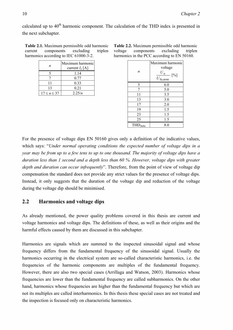
Electricity standards are also published by national authorities. Examples of these are Finnish Standards Association (SFS) and American National Standards Institute (ANSI). Examples of power quality standards published by these organisations are SFS-EN 50160, which is based on the European standard EN 50160, and ANSI C82.77-2002, which deals with the harmonics of lighting equipment. Power quality may be degraded in several ways. For example, the voltage quality of the distribution system is defined by the European standard EN 50160. The standard defines the main characteristics of supply voltage in the PCC in normal operating conditions and also describes the disturbances which may occur. In normal operating conditions, possible problems in the quality of the distribution voltage are wrong frequency or magnitude of the fundamental component or too high harmonic content. The three-phase voltage may also be unbalanced. Possible disturbances which may occur are e.g. supply interruptions, transient overvoltages, supply voltage dips and flicker. Quality problems may also occur in the currents of an electrical system. The main problem in current quality is the presence of harmonics. However, in this thesis only a few of these power quality problems are treated. Attention is paid mainly to current harmonics. This is because in this thesis the current harmonics filtering performance of three SHAPFs is compared. In addition to this, voltage harmonics and voltage dips are also treated, since the voltage harmonics filtering performance and voltage dip compensation performance of the UPQC are researched. The standards which concern harmonics and which are applicable from the point of view of this thesis are IEC 61000-3-2 and EN 50160. IEC 61000-3-2 defines the limits for harmonic current emissions for equipment with input current smaller than 16 A. This standard may be applied to a comparison of the current harmonics filtering performance of SHAPFs since it can be used as a reference point of the comparison. However, it has to be noticed that in this case the inspected current level is low since the comparison of the SHAPFs is based on the test results of low power laboratory prototypes. In real devices the current level may be higher, and if the current value 16 A is exceeded, IEC 61000-3-4 should be referred to instead of IEC 61000-3-2. EN 50160 defines the characteristics of the supply voltage in low-voltage distribution systems. This standard can be applied to the inspection of the operation of the UPQC since it is used to decrease the harmonic content of the supply voltage and to compensate the voltage dips described in this standard. Table 2.1 shows the limits of odd harmonic current components excluding the triplen harmonics according to IEC 61000-3-2. In Table 2.2 the maximum permissible odd harmonic voltage components excluding triplen harmonics in the PCC are presented according to EN 50160. In addition to the limits of harmonic voltage components, EN 50160 also specifies the maximum permissible value of the total harmonic distortion (THD) of the distribution voltage
10 Chapter 2
calculated up to 40th harmonic component. The calculation of the THD index is presented in the next subchapter.
Table 2.1. Maximum permissible odd harmonic current components excluding triplen harmonics according to IEC 61000-3-2.
n Maximum harmonic current In [A]
5 1.14 7 0.77
11 0.33 13 0.21
17 ≤ n ≤ 37 2.25/n
Table 2.2. Maximum permissible odd harmonic voltage components excluding triplen harmonics in the PCC according to EN 50160.
n
Maximum harmonic voltage
nomfu,UU n [%]
5 6.0 7 5.0
11 3.5 13 3.0 17 2.0 19 1.5 23 1.5 25 1.5
THD2kHz 8.0 For the presence of voltage dips EN 50160 gives only a definition of the indicative values, which says: “Under normal operating conditions the expected number of voltage dips in a year may be from up to a few tens to up to one thousand. The majority of voltage dips have a duration less than 1 second and a depth less than 60 %. However, voltage dips with greater depth and duration can occur infrequently”. Therefore, from the point of view of voltage dip compensation the standard does not provide any strict values for the presence of voltage dips. Instead, it only suggests that the duration of the voltage dip and reduction of the voltage during the voltage dip should be minimised.
2.2 Harmonics and voltage dips
As already mentioned, the power quality problems covered in this thesis are current and voltage harmonics and voltage dips. The definitions of these, as well as their origins and the harmful effects caused by them are discussed in this subchapter. Harmonics are signals which are summed to the inspected sinusoidal signal and whose frequency differs from the fundamental frequency of the sinusoidal signal. Usually the harmonics occurring in the electrical system are so-called characteristic harmonics, i.e. the frequencies of the harmonic components are multiples of the fundamental frequency. However, there are also two special cases (Arrillaga and Watson, 2003). Harmonics whose frequencies are lower than the fundamental frequency are called subharmonics. On the other hand, harmonics whose frequencies are higher than the fundamental frequency but which are not its multiples are called interharmonics. In this thesis these special cases are not treated and the inspection is focused only on characteristic harmonics.

Power quality problems and power filters 11
The harmonic contents of the signals may be inspected component by component. However, if the inspected frequency band is wide, this requires a considerable amount of work. The harmonic content of the inspected signal may also be presented using a single parameter. One method to do this is calculation of the total harmonic distortion (THD) index (Arrillaga and Watson, 2003; Mohan et. al., 1995). The THD index is defined as follows:
fu
2
2
THDI
Ik
nn∑
== , (2.1)
where Ifu is the RMS value of the fundamental current component, I2… Ik are the RMS values of the harmonic current components and k is the ordinal number of the highest harmonic component which is included in the calculation. Although (2.1) presents the calculation of the THD index of the current signal, the THD index of the voltage signal can be calculated respectively. In this thesis the THD indices are calculated either up to 2.5 kHz (50th harmonic component) or up to 20 kHz (400th harmonic component). The THDs are calculated up to the 50th harmonic component instead of the 40th, as specified by European standard EN50160, for the following reasons. First, it was desired that both current and voltage THDs be calculated up to the same harmonic component. The commercial companies that sell APFs, for example ABB and Areva T&D (former Nokian Capacitors), promise that their devices are able to filter current harmonics up to the 50th harmonic component, and it was therefore desired that this same limit be used in the current THD calculation (ABB, 2007; Nokian Capacitors, 2006). The reason why this limit is used by these companies is probably that some standards, such as IEC 61000-2-4, specify that the THD should be calculated up to the 50th harmonic component. In addition to this it must be noted that if there is a voltage waveform whose THD fulfils the requirement of EN50160 in the case where the THD is calculated up to the 50th harmonic component, then the THD of the waveform also has to fulfil the requirement if it is calculated only up to the 40th harmonic component, as is specified by this standard. The reason for calculating the THD up to the 400th harmonic component is that in this way the harmonics at the switching frequency of the inverter can be included in the inspection of the simulation and measurement results. Harmonics are created mainly due to nonlinear loads, which take harmonic currents from the supply (Bollen, 1999). The importance of harmonics as a power quality problem has increased since the 1970’s because the amount of switched power electronic devices, such as adjustable speed drives, uninterruptible power sources and ac/dc power supplies has increased in domestic, industrial and commercial environments (Akagi, 1996; Akagi, 2000; Bollen, 1999; El-Saadany, 2001; Peng, 2001; Zobaa, 2004). The popularity of switched power electronic devices is based on their advantages over traditional solutions, which are e.g. higher energy efficiency, improved equipment reliability, enhanced product quality, reduced product waste

12 Chapter 2
and reduced noise level (Bhattacharya and Divan, 1995; Domijan and Embriz-Santander, 1992). However, in addition to nonlinear loads there are various other sources of harmonics such as arc furnaces, fluorescent lamps and transformers (Arrillaga and Watson, 2003; Lai and Key 1997; Sueker et. al. 1989). Harmonics have numerous harmful effects on network components. According to Domijan and Embriz-Santander (2002), El-Saadany (2001), Lai and Key (1997) and Sueker et. al. (1989), these are e.g.:
• Production of pulsating and oscillating torques in turbines and generators. • Increasing of stator and rotor iron and copper losses in motors. • Increasing of eddy-current and hysteresis losses in transformers and inductors. • Increasing of reactive power in capacitors. Also additional heating occurs because of
increasing dielectric losses, which decreases the life expectancy of the capacitors. • Additional heating in cables because of skin and proximity effects. • False breaker tripping or fuse blowing. • Flickering of lights. • Interferences in communication circuits and other EMI-related problems.
The amount of harmonics can be reduced by using harmonic current filters, which are presented later in this chapter. The supply voltage dip is a reduction in the supply voltage, which lasts for a short time. EN 50160 gives the following description: “A sudden reduction of the supply voltage to a value between 90 % and 1 % of the declared voltage, followed by a voltage recovery after a short period of time. Conventionally the duration of a voltage dip is between 10 ms and 1 minute.”. Voltage dips are mainly caused by faults in the electrical system and when starting large motors (Bollen, 1999; Lamoree et. al., 1994). The existence of voltage dips in the electrical system is a serious problem, since they may generate high economic losses (Nam et. al., 2004; Sullivan et. al., 1997). The tolerances of devices connected to the supply network against voltage dips are not similar. In addition to this, the tolerance of each device against voltage dip depends on the duration of the dip and the magnitude of the voltage during the dip. This dependency can be presented using the voltage tolerance curve (Bollen, 1999; Djokić et. al., 2005). For example, the Information Technology Industry Council in the USA has published a voltage tolerance curve for information technology equipment (ITIC, 2000). Since the sensitivity of the electrical devices is different against voltage dips with different duration and magnitude, also the harmful effects caused by voltage dips depend on the

Power quality problems and power filters 13
duration and amplitude of the voltage during the dips. In general, typical disadvantages caused by the voltage dips are e.g. (Bollen, 1999; Djokić et. al., 2005; Lamoree et. al., 1994):
• Resetting or tripping of consumer electronics or domestic appliances. • Shutting down or restarting of computer-controlled industry processes. • Tripping of the adjustable speed drives due to the operation of their voltage
protection circuits. • Torque and speed variations in the motors. • Flickering of lights.
Voltage dips can be mitigated by using a voltage compensator between the supply and the equipment that is to be protected against voltage dips. Voltage compensators, which are used to compensate voltage dips, are e.g. an uninterruptible power supply (UPS), a dynamic voltage restorer (DVR) and the UPQC. The functioning of the UPQC is researched in the Section 2.5.2.
2.3 Passive filters
Passive filters have traditionally been used in current harmonics filtering in distribution networks at low or medium voltage level due to their simplicity, low cost and high efficiency (Bhattacharya and Divan, 1995; Das, 2004; El-Saadany, 2001). There are a variety of passive filter types: single-tuned, double-tuned, automatically tuned, damped and band-pass filters (Arrillaga and Watson, 2003; Domijan and Embriz-Santander, 1992). The most used passive filter types are single-tuned (LC shunt circuit) and damped (high-pass filter) passive filters. The single phase circuits of these two passive filters are presented in Figs. 2.1 and 2.2.
Fig. 2.1. LC shunt circuit. Fig. 2.2. High-pass filter.
The LC shunt circuit is a series LC circuit, which is connected in parallel with the power network. Its resonance frequency is tuned close to the frequency to be filtered. At the resonance frequency, the reactances of the inductor and the capacitor are equal and opposite, and thus the impedance of the filter is equal to its resistance. Because of the low impedance, harmonic currents near the resonance frequency flow through the LC shunt circuit instead of the supply and thus the harmonic content of the supply network decreases. The functioning principle of the high-pass filter is similar to the LC shunt circuit. However, compared to the LC shunt circuit, the high-pass filter includes an additional resistor connected

14 Chapter 2
in parallel with the inductor. The purpose of this resistor is to increase the pass band of the filter by passing through the harmonic currents above the resonance frequency. Passive filters have been used in current harmonics filtering because of their many advantages. These are e.g. (Bhattacharya and Divan, 1995; Das, 2004; El-Saadany, 2001):
• Simple implementation. • More economical implementation compared to APFs. • High efficiency. • Implementation in medium power level is possible. • Small amount of maintenance is needed. • Insensitiveness to disturbances and EMI-problems. • A single passive filter can serve many purposes, such as harmonic filtering, reactive
power compensation and current inrush support. However, passive filters also have several drawbacks. These are e.g. (Bhattacharya and Divan, 1995; Das, 2004; El-Saadany, 2001; Rivas et. al., 2002; Wang et. al., 2001):
• Large size. • Fixed compensation characteristics. • Tuning frequency may be changed due to ageing, deterioration and temperature
changes of the components. • Supply impedance strongly influences the filtering characteristics. • Susceptibility to series and parallel resonances with supply and other compensation
equipment connected to the system. • Sensitiveness to component tolerances and system configuration changes. • Susceptibility to load and line switching transients. Because of this, passive filters
are always off-tuned, which defeats their purpose as harmonic sinks. • High losses in high-pass configurations. • Stepless control is not possible.
2.4 Active power filters
Active power filters (APF) are based either on pulse-width modulated voltage or current source inverter (PWM-VSI, PWM-CSI) and are connected to the distribution system at low or medium voltage level (Fujita and Akagi, 1991; Morán et. al., 1999). Two main topologies of APFs exist: the parallel active power filter (PAPF) and series active power filter (SAPF) (Akagi, 1996). The development of APFs began in the 1970’s due to the development of power electronics technology (Akagi, 1996). One of the first ideas of active filtering was presented by Sasaki and Machida (1971). In that publication they presented a basic operating principle of a “new

Power quality problems and power filters 15
method to remove the harmonic currents”, i.e. the term “active power filter” was not yet used. The presented method of current harmonics removal was based on the injection of current harmonics, i.e. their device was basically the PAPF. In harmonics injection, a transformer with tertiary windings was used. Three years later they also published the simulation results which demonstrated the functioning of the presented method in steady-state operation and during current transients (Sasaki and Machida, 1974). Early research work considering active power filters was also presented by Gyugyi and Strycula (1976). In their publication the term “active power filter” was already used. In this article they presented the basic operating principles of the PAPF and SAPF. However, this article is significant because it also presents the practical realisations of APFs using fully controllable semiconductor switches. In addition to this, the article also presents the measurement results of the PAPF prototype. In the PAPF prototype a hysteresis based control system was used. A year after this, an article written by Mohan et. al. (1977) was published. This article presented the operating principle of the PAPF connected to LC shunt circuit. The simulation results of the presented PAPF were also provided. One of earliest practical realisations of APFs was published by Kawahira et. al. (1983). The publication was about the PAPF which was connected to a 6.6 kV distribution line for seven months in order to reduce the current harmonics. The development of APFs was continued in the 1980’s, when e.g. space vector calculation was applied to their control systems (Akagi et. al., 1984; Takeda et.al., 1987). Based on the above discussion it can be stated that APFs are a rather new invention. However, growing interest in APFs is based on the fact that most of the problems associated with passive filters, which have been used earlier in current filtering, can be solved using APFs. Therefore they have become a real alternative for passive filters in low and medium voltage systems. This is especially the case when for some reason (stiff supply, capacitive or variable load, etc.) it is difficult to design a passive filter (Bhattacharya and Divan, 1995; Johnson, 2002). The advantages of APFs are (Akagi, 1996; Akagi, 2000; Bhattacharya and Divan, 1995; Morán et. al., 1999; Peng, 2001; Wang et. al., 2001):
• Several functions can be provided using a single filter, e.g. reactive power compensation, harmonic filtering, flicker and imbalance compensation and voltage regulation.
• Compact size. • Controllable compensation characteristics. • Non-susceptibility to resonances. • Stepless control characteristics.

16 Chapter 2
However, APFs also have some drawbacks. These are e.g. (Fujita and Akagi, 1991; Bhattacharya and Divan, 1995; Massoud et. al., 2004; Peng et. al., 1990):
• Expensive price compared to passive filters. • Implementation of the PAPF is difficult at medium voltage level. • Worse efficiency than with passive filters.
2.4.1 Parallel active power filter
The PAPF is generally used for current harmonics filtering, reactive power compensation, balancing of unbalanced load currents and damping of resonances in the distribution systems at low voltage level (Akagi, 2000; El-Habrouk et. al., 2000). In Fig. 2.3, the PAPF is connected to the main circuit, which consists of the supply and the load. The PAPF consists of a converter and an output filter, which is of L or LCL type, and it is connected in parallel with the harmonics producing load. In addition to this, the PAPF may be connected to the main circuit also using a coupling capacitor or a step-down transformer.
Load
APF
isup ilo
ipfSupply
Fig. 2.3. Parallel active power filter.
The functioning principle of the PAPF in current harmonics filtering is to produce a compensation current ipf, which is inversely proportional to the load current harmonics ilo,h
(Bhattacharya and Divan, 1995; Morán et. al., 1999; Peng, 2001). Since the currents of the PAPF and the load are equal and opposite at the harmonic frequencies, they cancel out at the point of common coupling resulting in the sinusoidal supply current isup. Traditionally, the PAPF has been more popular in current harmonics filtering compared to the SAPF (Akagi, 1996; El-Habrouk et. al., 2000). This is because its filtering performance is better in cases where the load impedance is high, which is the case in the majority of the industrial loads, such as thyristor controlled rectifiers, cycloconverters, etc. (Akagi, 2000; Peng, 1998). When the load impedance is high, the load current is quite independent on the supply impedance and thus it is not changed due to the current injection of the APF. However, in cases where the load impedance is very low, such as with adjustable speed drives (ASD) with a capacitive dc-link, the compensation characteristics of the PAPF are dependent on the supply impedance (Peng, 1998). Since the compensation current ipf produced by the converter is divided between the supply and load branches in the ratio of their impedances, in

Power quality problems and power filters 17
the case of low load impedance this means that the majority of the current produced by the converter flows to the load and thus a very large compensation current ipf has to be produced by the converter in order to achieve an acceptable filtering performance. Therefore, in cases where the load impedance is low, the use of the PAPF in current harmonics filtering leads to an increase of the load current ripple and a large compensation current ipf is required from the APF (Peng, 1998). The second defect of the pure PAPF is its poor suitability in medium voltage applications. Because the PAPF is connected in parallel with the system, a high voltage rating of the converter is required since it has to produce a large fundamental component of the output voltage in order not to generate the large fundamental component of the compensation current ipf,fu. In the cases where the PAPF is used in medium power applications, cascade-connected converters, a multilevel converter, coupling capacitor or step-down transformer has to be used to match its voltage rating with that of the power network (Massoud et. al., 2004; Peng, 2001).
2.4.2 Series active power filter
The SAPF is generally used in current harmonics filtering and the compensation of voltage distortions, such as voltage dips, flicker and unbalanced three-phase voltages in the distribution systems at low and medium voltage levels (Akagi, 1996; El-Habrouk et. al., 2000; Karthik and Quaicoe, 2000; Rivas et. al., 2002). In Fig. 2.4, the SAPF is connected to the main circuit, which consists of the supply and the load. The SAPF consists of a converter, an output filter, which is of L or LC type, and a coupling transformer. The SAPF is connected in series between the supply and the load.
Load
u2
APF
isup
usf
usupulo
Supply
Fig. 2.4. Series active power filter.
In current harmonics filtering the converter produces an output voltage usf that is proportional to the supply current harmonics isup,h (Morán et al., 1999; Peng, 2001). The output voltage u2 is seen on the secondary side of the coupling transformer in proportion of the transformation ratio of the coupling transformer. Now, the secondary side voltage u2 of the coupling transformer is proportional to the current flowing through it and the coupling transformer can be seen as so-called active resistance at the harmonic frequencies. The supply current harmonics are decreased because of the increasing of the supply impedance at the harmonic
18 Chapter 2
frequencies due to the active resistance. As was the case with the PAPF, the current harmonics filtering characteristics of the SAPF are also dependent on the load impedance. The filtering performance of the SAPF is good in cases where the load impedance is low, i.e. the load current is more dependent on the supply impedance (Akagi, 1996; Peng, 1998; Rivas et. al., 2002). Only in these cases can the impedance seen by the load current harmonics be significantly increased by the active resistance. On the other hand, the SAPF is ineffective in harmonics filtering in cases where the load impedance is high (Peng, 1998). This is because in these cases a high output voltage u2 would be needed to produce notable active resistance compared to the load impedance. As was mentioned, the SAPF is also used in voltage harmonics filtering and voltage dip compensation. In these cases the role of the SAPF is different compared to current harmonics filtering since the purpose of the SAPF is to protect sensitive loads against disturbances in the supply voltage usup. In this case the SAPF produces compensation voltage u2, which is inversely proportional to the supply voltage distortions (Cheng et. al., 2003). Since u2 is inversely proportional to the supply voltage distortions, the distortions are cancelled, resulting in sinusoidal load voltage ulo. When the device is used for voltage dip compensation, it is also called a dynamic voltage restorer (DVR) instead of SAPF (Acha et. al, 2002; Bollen, 1999). The benefit of the SAPF is that it can also be used in medium voltage applications since the current and voltage ratings of its converter can be matched with ones of the supply network with the coupling transformer (Doležal et al., 2000). In this way the power rating of the converter can be designed to be as low as only a few per cent of the power rating of the load (Bhattacharya et. al., 1997; Doležal et al., 2000; Fujita and Akagi, 1991).
2.5 Hybrid active power filters
Since the invention of APFs, also hybrid active power filters (HAPFs) have been researched (see e.g. Takeda et. al., 1987). HAPFs consist of APFs and passive filters and they are divided into three categories. HAPFs that consist of APF and passive filters are called either parallel hybrid active power filters (PHAPFs) or series hybrid active power filters (SHAPFs), depending on the type of APF used (Akagi, 1996; Peng, 2001). A HAPF consisting of both PAPF and SAPF is called unified power quality conditioner (UPQC) (Fujita and Akagi, 1996). As one might guess, numerous HAPF topologies exist, e.g. in (Peng, 2001) 18 different PHAPF and SHAPF topologies are presented. The aim in HAPF design is to mitigate the problems associated with pure APFs and passive filters and to complement or enhance their performance by adding active or passive components to their structure (Bhattacharya and Divan, 1995; Peng, 2001). HAPFs have the

Power quality problems and power filters 19
following advantages compared to passive filters (Akagi, 2000; Bhattacharya and Divan, 1995; Bhattacharya et. al., 1997; Morán et. al., 1999; Peng et. al. 1993):
• Better filtering performance. • Controlled compensation characteristics. • Non-susceptibility to resonances. • Compensation characteristics are less dependent on supply impedance. • Several compensation features, such as harmonic filtering, supply voltage regulation,
imbalance compensation and reactive power compensation are provided by a single filter.
Furthermore, HAPFs have the following advantages compared to APFs (Bhattacharya and Divan, 1995; Fujita and Akagi, 1991; Rivas et. al., 2002; Rivas et. al., 2003):
• Smaller cost. • Smaller converter power rating. • Implementation at medium voltage level is possible.
2.5.1 Parallel and series hybrid active power filters
As was already mentioned, there are numerous PHAPF and SHAPF topologies. Since it is not possible to present them all, an example of each filter is given. In Figs. 2.5 and 2.6 the most typical examples of PHAPF and SHAPF are presented.
Load
APF
isup ilo
ipf ihp
Supply
Load
u2
APF
isup
i5
ilo
usf
Supply
Fig. 2.5. Parallel hybrid active power filter. Fig. 2.6. Series hybrid active power filter.
In Fig. 2.5, the harmonic currents produced by the load are filtered using both the PAPF and passive filter. The idea of using two filters is to share the compensation bandwidth between the PAPF and passive filter. Low-order harmonics are filtered using the PAPF and high-order harmonics using the passive filter (Takeda et. al., 1987). Because of this, a lower switching frequency of the converter switches is required and thus the switching losses are decreased compared to the pure PAPF. In addition to this, the dimensions of the passive filter are smaller than in the normal case, where the resonance frequency of the passive filter is tuned near characteristic low-order harmonics (5th or 7th harmonic frequency) since the tuning frequency of the passive filter is high.

20 Chapter 2
In the topology shown in Fig. 2.6, the passive filter is used to filter load current harmonics. The SAPF is used to produce active resistance in series with the supply. Because of the active resistance produced by the SAPF, the impedance of the supply branch increases at the harmonic frequencies. Because of this, harmonic currents flow in the passive filter more effectively than when only the passive filter is used (Morán et. al., 1999; Peng, 2001; Rivas et. al., 2002).
2.5.2 Unified power quality conditioner
The unified power quality conditioner (UPQC) consists of the PAPF and SAPF, which have a common dc-link (Akagi et. al., 2007). In Fig. 2.7, the UPQC is connected to the main circuit, which consists of the supply and load.
Load
u2
APF
isup ilo
ipm
usf
Supply
usupulo
ipf
Fig. 2.7. Unified power quality conditioner.
Since the UPQC is made of the PAPF and SAPF, it combines their compensation characteristics. The SAPF can be used to filter supply voltage harmonics and to compensate supply voltage deviations, such as voltage dips, flicker, etc. The PAPF is used to filter load current harmonics and to compensate the reactive power. Since the UPQC is capable of compensating both current and voltage deviations, it is regarded as the most sophisticated power quality conditioner (Acha et. al., 2002; Akagi, 1996; Fujita and Akagi; 1996; Peng, 2001). The main circuit of the UPQC is very similar to the main circuit of the unified power flow controller (UPFC), which is used in power flow control at fundamental frequency in transmission systems (Akagi et. al., 2007; Acha et. al., 2002; Gyugyi et. al., 1995). The only difference is that in the UPFC the parallel-connected converter is on the supply side and series-connected converter on the load side. In addition to this, since the UPFC is used in the transmission systems and the UPQC in distribution systems, their practical realisations differ because of different voltage and power ratings. In addition to the close relation to UPFC, the main circuit of the UPQC is also very close to the series-parallel line-interactive uninterruptible power supply (UPS) (da Silva et. al., 2002, Emadi et. al., 2005). This UPS is also called a delta-conversion UPS (Dai et. al., 2003). This

Power quality problems and power filters 21
kind of device is presented in Fig. 2.8.
Load
u2
UPS
isup ilo
usf
ulo
Supply
usup
ipm
ipf
Fig. 2.8. Series-parallel line-interactive UPS.
As can be seen by comparing Figs. 2.7 and 2.8, the only differences between the main circuits of the UPQC and the delta-conversion UPS are the switch between the supply and the coupling transformer and the battery bank connected to the dc-link. However, despite similar main circuits, their control principles are slightly different. The functioning of the UPS is as follows. In standby operation, i.e. when the supply is at normal condition, the switch is closed and the load is fed from the supply. The series-connected converter (i.e. the SAPF) is used to make the supply current sinusoidal and to charge the battery bank connected to the dc-link (da Silva et. al., 2002). The function of the parallel-connected converter is to compensate the load voltage fluctuations and therefore to provide sinusoidal voltage to the load (da Silva et. al., 2002). If the supply voltage usup is beyond the specified limits, the switch is opened. The load voltage ulo is now maintained using the parallel-connected converter. This means that the load is fed by the parallel-connected converter, which takes the energy from the battery bank connected to the dc-link. Since the load is fed by the parallel-connected converter, the series-connected converter is not operated and its output voltage is equal to zero. If the operation of the UPQC and the series-parallel line-interactive UPS is compared, it can be stated that their functioning is quite similar if the supply voltage is inside the specified limits. In both cases the purpose of the device is to make the supply currents and load voltages sinusoidal. Of course, since the battery bank is not included in the dc-link of the UPQC, there is no need to charge it. However, their functioning is different when the supply voltage is beyond the specified limits. The UPQC is able to maintain the load voltage as long as there is enough energy in the dc-link capacitor, which is charged by the PAPF. Therefore, the operation of the UPQC is dependent on the state of the supply. As long as there is some voltage in any phase of the supply, the PAPF can charge the dc-link voltage capacitor and the UPQC is able to operate. If there is a complete three-phase supply voltage interruption, the UPQC shuts down in a fraction of a fundamental cycle. However, the UPS is not dependent on the supply and is able to operate also during supply voltage interruptions because the battery bank is connected to
22 Chapter 2
the dc-link. The operation time of the UPS is not infinite, but is defined by the load that is fed and the capacity of the battery bank. Typical maximum operation times are of the order of tens of minutes to some hours (Emadi et.al., 2005).
2.6 Commercial SAPF based filters and their applications
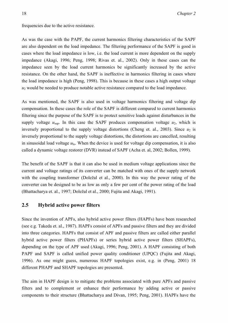
This chapter briefly presents commercial SAPF based filters and their applications. The pure SAPF, which is used in current harmonics filtering, is still at the experimental stage and commercial versions can not be found. This is due to two reasons. First, as was earlier mentioned, the current harmonics filtering performance of the SAPF is poor when the load impedance is not low. Second, the SAPF is more expensive than the PAPF. It is calculated that the expenses of the SAPF are approximately 1.5 times higher than those of the PAPF (Lai and Key, 1997). However, the SAPF is widely used in voltage compensation, such as compensation of the voltage dips, flicker and voltage unbalance. As earlier stated, in this case it is called the DVR. However, the manufacturers of the DVRs also use names such as “active voltage conditioner”, “voltage conditioner”, “power conditioner”, “line conditioner”, “voltage regulator” and “sag ride through”. This makes the situation rather confusing, since basically these terms are used to describe the same device, although there may be slight differences, e.g. in the implementation of the dc-link of the device between manufacturers. In addition to DVRs, also some SAPF based filters, such as the UPQC and the delta-conversion UPS, are commercially available. Some commercially available DVRs are next presented. The information about the devices presented in this chapter was mainly gathered from manufacturers’ websites, which are presented at the end of the references. In addition to this, some information was also received directly from manufacturers, who were contacted by e-mail and phone. One manufacturer of DVRs has been ABB Ltd., which, however, does not produce them anymore. Therefore the specifications of their DVRs are not available. However, from the internet some ABB application notes concerning DVRs can be found. One of them presents the DVR which was installed in Quiriat Gat, Israel, in August 2000. The DVR is presented in Fig. 2.9. The DVR consists of two 22.5 kVA units, which were connected to 22 kV line to protect the production facility of a microprocessor manufacturer against voltage dips. The DVR is able to compensate a three phase voltage dip of 35 % of the nominal voltage.

Power quality problems and power filters 23
Fig. 2.9. The interior of ABBs 22.5 MVA DVR made inside a freight container. The picture is reprinted with the permission of ABB Ltd.
Eaton Corporation provides DVRs which are used to compensate voltage dips. These devices are able to compensate three-phase voltage sags down to 40 % of the nominal voltage. The DVRs are available in power ratings between 25 kVA and 4 MVA. Depending on the device, they can be connected to low or medium voltage up to 15 kV. Omniverter Inc. is the North American partner of Vectek Electronics and provides DVRs with two different voltage ratings. The DVRs for low voltage networks are manufactured with power ratings from 25 kVA to 6 MVA. The DVRs for medium voltage networks with rated voltage below 38 kV are manufactured with power ratings from 1 MVA up to 50 MVA. All DVRs are able to compensate voltage dips, unbalanced voltages and flicker. The DVRs are able to compensate three-phase voltage dips down to 50 % of the nominal voltage. S&C Electric Company manufactures DVRs intented to mitigate voltage dips and disturbances occurring in the supply. The design of the DVR is modular. The power rating of each module is 2 MVA and it can be connected to voltage between 3.3 kV and 72.5 kV. An appropriate amount of modules is used to achieve the necessary compensation capacity. In this fashion, the compensation capacity can be increased to 10 MVAs. Vectek Electronics manufactures DVRs which are capable of compensating voltage dips, voltage unbalance and flicker. The DVRs are intended to be connected to low voltage, although there are medium voltage options available as custom design. The power ratings of the standard DVRs are between 160 kVA and 2.4 MVA. The power rating may be increased up to 10 MVA in the custom designs. The DVRs are capable of compensating three-phase voltage dips smaller than 30 % of the nominal voltage.

24 Chapter 2
Next, a SHAPF implementation and two commercial SAPF based filters are presented. Bhattacharya and Divan (1995) present a real-life SHAPF implementation. The power rating of the SAPF is 35 kVA and it is installed at a wastewater pump station in Beverly, MA, USA. The purpose of the SHAPF is to filter the current harmonics generated by the four ASDs whose total power rating is 765 kVA. Unfortunately, the reference does not reveal the manufacturer of the SAPF. American Power Conversion Corporation (APCC) offers a whole series of delta-conversion UPSs, which is called “the Silcon series”. These UPSs are available in the power ratings from 60 kVA up to 480 kVA. The UPSs are intended to be connected to the three-phase system with 230/400 V nominal voltage. Silcon series UPSs are able to filter current and voltage harmonics, compensate the reactive power and regulate the voltage. The Silcon series UPSs are also able to feed the load during supply interruptions from some minutes to nearly 24 hours depending on the power ratings of the UPS and the load. Hykon Group manufactures UPQCs, which are made of a back-to-back connected static compensator (STATCOM) and the DVR. The UPQCs are available in the range of 10 kVA to 250 kVA and are connected to a low voltage level. The information about SAPF based filters, which was presented above, is summarised in Table 2.3.
Table 2.3. Commercially available and real implementations of SAPF based filters.
Filter type Manufacturer Switch type Power rating
Phase to phase voltage in the
point of connection
Filtering / compensation
type**
DVR ABB Ltd. IGCT 22.5 MVA 22 kV 2 DVR Eaton Corp. IGBT 25 kVA – 4 MVA 208 V– 15kV 2 DVR Omniverter Inc. (Vectek El.) - 25 kVA – 6 MVA 206 V – 690 V 2 DVR Omniverter Inc. (Vectek El.) IGBT 1 MVA – 50 MVA 2.4 kV – 38 kV 2 DVR S&C Electric Company - 2 MVA – 10 MVA 3.3 kV – 72.5 kV 2 DVR Vectek Electronics IGBT 160 kVA – 2.4 MVA 208 V – 600 V 2 SHAPF Unknown IGBT 35 kVA 480 V 1 UPQC Hykon Group IGBT 10 kVA – 250 kVA 415 V 2,3 UPS* APCC IGBT 60 kVA – 480 kVA 400 V 1,2,3
* = delta-conversion UPS. ** = The types are divided into the following categories: 1 = Current or voltage harmonics filtering. 2 = Voltage regulation (voltage dip compensation, three-phase voltage balancing etc.) 3 = Reactive power compensation.
Based on the previous table it can be seen that SAPF based filters can be used at different voltage and power levels. The power ratings of the DVRs, UPQC and delta-conversion UPS are rather high since in these devices the SAPF is used for voltage compensation. If there is, e.g. a supply voltage dip, the SAPF has to produce a missing load voltage and therefore it

Power quality problems and power filters 25
partially feeds the load. If the power of the load is high and voltage dips with low remnant voltage needs to be compensated, the power rating of the series compensation device has to be high. On the other hand, in the case of the SHAPF, where the SAPF is used for current harmonics filtering, its power rating can be kept relatively small compared to the power of the load. This is the benefit of the SAPF, i.e. the power rating of the SAPF can be designed to be significantly smaller than that of the load while the filtering performance of the SAPF is designed to be good. Another benefit of the SAPF, which concerns all filters shown in Table 2.3, is that the SAPF can also be used at the medium voltage level because it is connected in series with the power network. The presented SAPF based filters are used in several applications. Based on the manufacturers’ websites, the typical application targets are the supply systems of industrial facilities (e.g. plastic film, paper or semiconductor manufacturing), hospitals and commercial buildings.

26 Chapter 3
3 Operating principles of SAPF based power filters
In this chapter, the main circuit structures and operating principles of the series active power filter (SAPF) and three series hybrid active power filters (SHAPFs) in current harmonics filtering are presented. In addition to this, the operating principle of the unified power quality conditioner (UPQC) in current and voltage harmonics filtering and voltage dip compensation is investigated. Since the control systems of the presented active power filters (APFs) are based on space vector calculation, the fundamentals of space vector theory are presented at the beginning of the chapter. In this work, the switching components of the inverters are modulated using space vector modulation, which is based on space vector theory. Space vector modulation is introduced after the space vector theory. After this, the main circuit structure and operating principle of SAPF in current and voltage harmonics filtering and voltage dip compensation is presented. Next, the main circuit structures and operating principles of three SHAPFs in current harmonics filtering are presented. The SHAPFs are a supply connected topology (SCT), a filter connected topology (FCT) and an electrically tuned LC shunt circuit (ETLC). The structures and the operating principles of the control systems of SHAPFs are also discussed. In the case of the SCT and the FCT, the influence of the dc-link voltage control on their filtering performance is inspected. Last, the main circuit and control system structures of the UPQC as well as their operating principles in current and voltage harmonics filtering and voltage dip compensation are presented. At the end of this chapter it is shown how control delay compensation is applied to the control system of the SAPF.
3.1 Space vector theory
Regardless of the APF type or topology, its control system has to be able to detect harmonic components from the measured signal in order to filter harmonics. The detection of the harmonic components can be done either in the frequency or time domain (Akagi, 1996; Emadi et. al., 2005; Grady et. al., 1990; Green and Marks, 2005). The frequency domain calculation of the harmonic components is based on Fourier analysis. In this kind of harmonic components detection the frequency components are calculated from the measured block of data using fast Fourier transformation (Grady et. al., 1990; Green and Marks, 2005; Mariethoz and Rufer, 2002). In the time domain the most used solutions are based either on

Operating principles of SAPF based power filters 27
instantaneous power theory (referred also as p-q theory) or on extraction of the harmonics in the rotating reference frame (Akagi, 1996, Akagi et. al., 2007; Bhattacharya and Divan, 1995; Emadi et. al., 2005; Rivas et. al., 2002). The implementations of the control systems, which are based on instantaneous power theory or on the extraction of the harmonics in the rotating reference frame are based on space vector theory which was proposed at the end of the 1950’s (Kovács and Rácz, 1959). Space vector calculation was originally used to model ac machines and was later applied to their control systems (Kovács and Rácz, 1959; Novotny and Lipo, 1996; Vas, 1992). After the invention of the APFs space vector calculation was also applied to their control systems. This took place at the beginning of the 1980’s (Akagi et. al., 1984). In the literature, two different definitions of the space vector can be found. Based on these different definitions, space vector transformation is called either power invariant or power non-invariant (Vas, 1992). The space vectors calculated based on these two different definitions are nearly identical. The only difference is that the lengths of the resulting space vectors are different. In this work, power non-invariant transformation is used. The fundamentals of the space vector theory are presented next (Vas, 1992). The space vector of an arbitrary three-phase variable xA, xB, xC in the stationary reference frame is defined as (Vas, 1992):
( )C2
BA aa32 xxxx ++= (3.1)
where
23j
21ea 3
π2j+−== (3.2)
In this work, the space vector in the stationary reference frame is denoted as x, i.e. no superscript is used. If the system includes a zero sequence component (i.e. the sum of the phase quantities xA, xB and xC differs from zero), it has to be taken into account separately.
( )CBA0 31 xxxx ++= (3.3)
The space vector consists of two perpendicular components, the first of which is parallel with the real axis and other one parallel with the imaginary axis. These components are referred to with the subscripts α and β in the stationary reference frame. βα jxxx += (3.4)
Based on (3.1) and (3.3), the following transformation matrix between the three-phase variables xA, xB and xC and the space vector components in the stationary reference frame can be derived (Vas, 1992):

28 Chapter 3
⎥⎥⎥
⎦
⎤
⎢⎢⎢
⎣
⎡
⎥⎥⎥
⎦
⎤
⎢⎢⎢
⎣
⎡−−−
=⎥⎥⎥
⎦
⎤
⎢⎢⎢
⎣
⎡
C
B
A
0
β
α
21212123230
21211
32
xxx
xxx
(3.5)
The transformation matrix for the calculation of the three-phase variables from the space vector representation can also be formulated by using matrix inversion.
⎥⎥⎥
⎦
⎤
⎢⎢⎢
⎣
⎡
⎥⎥⎥
⎦
⎤
⎢⎢⎢
⎣
⎡
−−−=
⎥⎥⎥
⎦
⎤
⎢⎢⎢
⎣
⎡
⎟⎟⎟
⎠
⎞
⎜⎜⎜
⎝
⎛
⎥⎥⎥
⎦
⎤
⎢⎢⎢
⎣
⎡−−−
=⎥⎥⎥
⎦
⎤
⎢⎢⎢
⎣
⎡−
0
β
α
0
β
α1
C
B
A
1232112321101
21212123230
21211
32
xxx
xxx
xxx
(3.6)
The control systems inspected in this work are based on space vector calculation in the rotating reference frame. Next it is shown how the space vector presented in the stationary reference frame is transformed to the rotating reference frame. The space vector can be presented in polar coordinates, i.e. by using its amplitude and angle as:
( )0je ϕ+= ωtxx , (3.7)
where t is time, ω is the angular speed of the space vector and ϕ0 is its angle at time instant t = 0. If now the reference frame rotating at arbitrary angular speed ωk is considered, the angular speed of the space vector in this reference frame is ω -ωk, i.e. assuming ϕ0 = 0, the space vector can be presented in the rotating reference frame as
tt exexx kk j)j(k ωωω −− == , (3.8)
where the superscript k refers to the reference frame rotating at arbitrary angular speed. This shows how the space vector transformation between the stationary and rotating reference frames is made. The inverse transformation is made using the following equation:
texx kjk ω= (3.9)
The vector components in parallel with the real and imaginary axis in the rotating reference frame are solved by using the Euler equation
tte t ωωω sinjcosj += . (3.10)
In this work, the following super/subscripts are used to denote the angular speed of the reference frame and the space vector and its components presented in this reference frame: reference frame rotating at the arbitrary angular speed: ωk, xk = xx + jxy, supply voltage oriented synchronous reference frame (or simply synchronous reference frame): ωs, xs = xd + jxq and reference frame rotating at the angular speed corresponding to the nth harmonic frequency component: ωn, xn = xn
d + jxnq.
As was shown in (3.8), the space vector presented in the stationary reference frame can be transformed in the reference frame rotating at arbitrary angular speed if the angular speed of the reference frame ωk is known. For example, the space vector components in the synchronous reference frame are calculated taking (3.10) account:

Operating principles of SAPF based power filters 29
⎥⎥⎥
⎦
⎤
⎢⎢⎢
⎣
⎡
⎥⎥⎥
⎦
⎤
⎢⎢⎢
⎣
⎡−=
⎥⎥⎥
⎦
⎤
⎢⎢⎢
⎣
⎡
0
β
α
ss
ss
0
q
d
1000cossin0sincos
xxx
tttt
xxx
ωωωω
(3.11)
The zero sequence component is independent of the reference frame. The opposite transformation from the rotating reference frame to the stationary reference frame is achieved using matrix inversion.
⎥⎥⎥
⎦
⎤
⎢⎢⎢
⎣
⎡
⎥⎥⎥
⎦
⎤
⎢⎢⎢
⎣
⎡ −=
⎥⎥⎥
⎦
⎤
⎢⎢⎢
⎣
⎡
⎥⎥⎥
⎦
⎤
⎢⎢⎢
⎣
⎡−=
⎥⎥⎥
⎦
⎤
⎢⎢⎢
⎣
⎡−
0
q
d
ss
ss
0
q
d1
ss
ss
0
β
α
1000cossin0sincos
1000cossin0sincos
xxx
tttt
xxx
tttt
xxx
ωωωω
ωωωω
(3.12)
Using (3.8), also the space vector transformation between two rotating reference frames may be defined. If the space vector xs = xd + jxq presented in the synchronous reference frame is transformed to the reference frame rotating at the angular speed corresponding to the nth harmonic frequency component, the vector components in this new reference frame are calculated as follows:
( )( ) ( )( )( )( ) ( )( )
⎥⎥⎥
⎦
⎤
⎢⎢⎢
⎣
⎡
⎥⎥⎥
⎦
⎤
⎢⎢⎢
⎣
⎡−−−−−
=⎥⎥⎥
⎦
⎤
⎢⎢⎢
⎣
⎡
0
q
d
ss
ss
0
q
d
1000cossin0sincos
xxx
tttt
xxx
nn
nnn
n
ωωωωωωωω
(3.13)
The opposite transformation between the reference frames is achieved using matrix inversion.
( )( ) ( )( )( )( ) ( )( )
( )( ) ( )( )( )( ) ( )( )
⎥⎥⎥
⎦
⎤
⎢⎢⎢
⎣
⎡
⎥⎥⎥
⎦
⎤
⎢⎢⎢
⎣
⎡−−−−−
=
⎥⎥⎥
⎦
⎤
⎢⎢⎢
⎣
⎡
⎥⎥⎥
⎦
⎤
⎢⎢⎢
⎣
⎡−−−−−
=⎥⎥⎥
⎦
⎤
⎢⎢⎢
⎣
⎡−
0
q
d
ss
ss
0
q
d1
ss
ss
0
q
d
1000cossin0sincos
1000cossin0sincos
xxx
tttt
xxx
tttt
xxx
n
n
nn
nn
n
n
nn
nn
ωωωωωωωω
ωωωωωωωω
(3.14)
The instantaneous real power in the three-phase system is calculated using the space vectors of the voltage u and current i as (Vas, 1992):
( ) ( )k*k* Re23Re
23 iuiup == (3.15)
3.1.1 Space vector modulation
The fundamental part of the APF is a pulse width modulated voltage source inverter (PWM-VSI). The main circuit of the three-phase PWM-VSI, which consists of six controllable switches, a dc-link capacitor Cdc and a discharge resistor Rdc is presented in Fig. 3.1.

30 Chapter 3
Cdc
idc
udc
usfA
usfB
usfC
isfA
isfB
isfC
Rdc
Fig. 3.1. Pulse-width modulated voltage source inverter.
The output terminals of the phases are connected to the positive and negative dc-voltages via controllable semiconductor switches. The operating principle of the PWM-VSI is to generate the pulse-width modulated output voltages usfA, usfB and usfC to its output terminals from the constant dc-link voltage udc. The PWM-voltages are created by switching the semiconductor switches in an on/off-fashion according to the reference values. Both of the switches connected to the same output terminal are never turned on simultaneously, because in this case a short circuit would occur. In addition to this, in real implementations the states of the switches are never changed simultaneously for the same reason. Instead, between the switching states there is always a short period of time when both switches are turned off. This period is called dead time. The dead times are not taken into account in the simulation models presented in this thesis. However, in the implemented prototype of the SAPF approximately 2.6 μs dead time is used. There are numerous methods to control the inverter switches in order to generate the pulse-width modulated output voltages. Examples of these methods are triangular carrier based sinusoidal pulse width modulation, space vector modulation and random modulation (Kazmierkowski et. al., 2002). In this work, (asymmetrical regularly sampled) space vector modulation, which is based on the space vector theory presented in the previous subchapter, is used (Holmes and Lipo, 2003). The fundamentals of space vector modulation are presented next (Holmes and Lipo, 2003; Ollila, 1993). First, the states of the inverter switches connected to the positive dc-link voltage are denoted as swA+, swB+ and swC+. Respectively, the states of the inverter switches connected to the negative dc-link voltage are denoted as swA-, swB- and swC-. Next, the states of the switches are defined as “1” when they are on and “0” when they are off. Now, if the mid-point of the dc-link voltage is used as a reference, the states of the output terminals, which are also called the switching functions of the phases, can be presented as:

Operating principles of SAPF based power filters 31
( ) 2AAA −+ −= swswsw (3.16)
( ) 2BBB −+ −= swswsw (3.17)
( ) 2CCC −+ −= swswsw (3.18)
As is seen, these switching functions have values ±(1/2) depending on the states of the switches. The space vector presentation of the switching functions is obtained using (3.1).
( )C2
BA aa32 swswswsw ++= (3.19)
On the other hand, the six switches of the inverter have eight possible combinations of switching states (Holmes and Lipo, 2003). Two of these switching states produce zero output voltage and thus these states are called zero states and the output voltage vectors corresponding to these switching states are called zero switching vectors. In the case of the remaining six switching states, non-zero output voltage is produced to the output terminals and therefore these states are called active states. In the case of active states the output voltage vectors are called active switching vectors. Based on (3.2) and (3.19), the space vector of the switching functions swA, swB and swC may be presented in active states as
( )
3π1j
e32 −
=i
isw (3.20)
where i is an integer 1…6. The phase voltages of the inverter can be presented by using the switching states and the dc-link voltage udc: dcAsfA uswu = (3.21)
dcBsfB uswu = (3.22)
dcCsfC uswu = (3.23)
The space vector presentation of the inverter output voltage is achieved using (3.19).
( ) dcdcC2
BAsf aa32 uswuswswswu =++= (3.24)
By combining (3.20) and (3.24) the output voltage vectors in the case of active states, i.e. the active switching vectors, are achieved.
( )
3π1j
dcdcsf e32 −
==i
ii uuswu (3.25)
These active switching vectors are presented in Fig. 3.2 with zero switching vectors usfz+ and usfz-. It can be seen that the amplitudes of the active switching vectors are the same and the phase difference between the adjacent vectors is 60°. These vectors divide the plane defined by the real and imaginary axes into six switching sectors denoted as I - VI. The first switching

32 Chapter 3
sector is presented more closely in Fig. 3.3.
Im
Reusf1
usf2usf3
usf4
usf5 usf6
usfz+ usfz-
I
II
III
IV
V
VI
Im
Reusf1
usf2
usfref
(t1/(Tmod/2))usf1
(t2/(Tmod/2))usf2
Fig. 3.2. Switching sectors and output voltage vectors.
Fig. 3.3. Realisation of output voltage reference vector usfref in the switching sector one.
Since the desired output voltage vector rarely matches with the active switching vectors, the output voltage is generated using two adjacent active switching vectors and both zero switching vectors. The duration of each switching combination during a half modulation period is calculated so that the average of the active switching vectors equals the output voltage reference vector. This is presented as follows.
1sfmod
1sf
modsfref 22 +
++= ii
ii u
Tt
uT
tu (3.26)
where ti is the duration of the active switching vector usfi, ti+1 is the duration of the active switching vector usfi+1 and Tmod is the modulation period. The durations of the active switching vectors are solved from the above equation by noticing that the phase difference between the adjacent active switching vectors is 60° (Ollila, 1993).
( )sfref1dc
sfrefmod sin
23 ϕϕ −= +ii u
uTt (3.27)
and
( )ii uu
Tt ϕϕ −=+ sfrefdc
sfrefmod1 sin
23 (3.28)
where ϕ sfref is the phase angle of the output voltage reference vector usfref and ϕ i and ϕ i+1 are the phase angles of the adjacent active switching vectors usfi and usfi+1 in respect of the positive real axis. The realisation of the output voltage reference vector with the adjacent output voltage vectors in switching sector one is illustrated in Fig. 3.3. The rest of the modulation period is fulfilled with the zero switching vectors usfz+ and usfz-. The combined duration of the zero switching vectors during a half modulation period, i.e. tz = tz+ + tz-, is calculated as follows.

Operating principles of SAPF based power filters 33
1mod
z 2 +−−= ii ttT
t (3.29)
The switches are operated symmetrically in order to achieve all switching combinations from the previous ones by changing the state of only one of the six switches. In this way the switching losses are minimised. In conclusion, the active switching vectors are presented in Table 3.1 and zero switching vectors in Table 3.2.
Table 3.1. Active switching vectors.
i usfA usfB usfC usf ∠usf 1 +udc/2 -udc/2 -udc/2 2/3udce0 0° 2 +udc/2 +udc/2 -udc/2 2/3udcejπ/3 60° 3 -udc/2 +udc/2 -udc/2 2/3udcej2π/3 120° 4 -udc/2 +udc/2 +udc/2 2/3udcejπ 180° 5 -udc/2 -udc/2 +udc/2 2/3udcej4π/3 240° 6 +udc/2 -udc/2 +udc/2 2/3udcej5π/3 300°
Table 3.2. Zero switching vectors.
usfA usfB usfC usf ∠usf z+ +udc/2 +udc/2 +udc/2 0 0° z- -udc/2 -udc/2 -udc/2 0 0°
The whole switching sequence during one modulation period in each switching sector is illustrated in Table 3.3, where k indicates the order of execution of the switching states.
Table 3.3. States of the switches during one modulation period.
Tmod Switching sector Time instant k k+1 k+2 k+3 k+4 k+5 k+6 k+7
Output voltage vector usfz- usf1 usf2 usfz+ usfz+ usf2 usf1 usfz- I Duration tz/2 t1 t2 tz/2 tz/2 t2 t1 tz/2 Output voltage vector usfz- usf3 usf2 usfz+ usfz+ usf2 usf3 usfz- II Duration tz/2 t3 t2 tz/2 tz/2 t2 t3 tz/2 Output voltage vector usfz- usf3 usf4 usfz+ usfz+ usf4 usf3 usfz- III Duration tz/2 t3 t4 tz/2 tz/2 t4 t3 tz/2 Output voltage vector usfz- usf5 usf4 usfz+ usfz+ usf4 usf5 usfz- IV Duration tz/2 t5 t4 tz/2 tz/2 t4 t5 tz/2 Output voltage vector usfz- usf5 usf6 usfz+ usfz+ usf6 usf5 usfz- V Duration tz/2 t5 t6 tz/2 tz/2 t6 t5 tz/2 Output voltage vector usfz- usf1 usf6 usfz+ usfz+ usf6 usf1 usfz- VI Duration tz/2 t1 t6 tz/2 tz/2 t6 t1 tz/2
3.2 Primary side connection of the coupling transformer
The compensation voltage produced by the SAPF is fed to the main circuit using the coupling transformer. Therefore, the phases of the secondary side of the coupling transformer are always connected in series with the main circuit. On the other hand, the primary side of the transformer can be either wye or delta-connected. However, the quality of the compensation voltage seen on the secondary side of the transformer may depend largely on the primary side

34 Chapter 3
connection. If the transformer is not well designed, the secondary side voltage is distorted if the primary side is wye-connected and three-wire connection is used. This phenomenon is discussed in this subchapter. In Figs. 3.4a and 3.4b are presented the connections of the transformer terminals in cases where the primary side is either wye- or delta-connected. The transformer is a three-phase transformer, which consists of three single-phase transformers. The positive terminals of the primary and the secondary sides are indicated using upper case letters and the negative terminals using lower case letters. When the primary side is wye-connected, the voltage over the primary side coil in phase-A is equal to phase to neutral voltage u1A. The neutral point voltage is denoted as uN and the secondary side voltage of phase-A as u2A. On the other hand, when the primary side is delta-connected, the voltage over the primary side coil in phase-A is equal to phase to phase voltage u1AB.
a)
1A
1au1A
2A
2au2A
2B
2C2b
2c
1b(uN)
1c
1B
1C
b)
1A
1au1AB
2A
2au2A
2B
2C2b
2c
1b
1c
1B
1C
Fig. 3.4. Transformer terminals: a) wye-connected primary side and b) delta-connected primary side.
The purpose of the coupling transformer is to generate the compensation voltage u2 on its secondary side. This compensation voltage should be a linear function of the voltage applied to the primary side terminals 1A, 1B and 1C. However, if the transformer is not designed carefully, the function between these voltages is not linear but is disturbed by the harmonic components which are caused by the non-linearity of the core (Matsch and Morgan, 1987). The linearity between these voltages depends on the transformer core material and on the transformer design (Matsch and Morgan, 1987; McPherson and Laramore, 1990; Van den Boscche and Valchev, 2005). In practice, this means that the linearity can be improved by choosing a core material, whose magnetic flux density has a higher level of saturation or the hysteresis is smaller. The linearity may also be improved by designing the transformer for lower value of maximum magnetic flux density. However, all of these ways to improve the linearity of the transformer also increase its manufacturing costs. Better core materials are more expensive and if the transformer is designed for lower value of the magnetic flux density, the physical size of the transformer is increased. In addition to the transformer design, the linearity of the three-phase coupling transformer of the SAPF also depends on the connection of the primary side windings. Let us consider the transformer connection shown in Fig. 3.4a, where the primary side of the transformer is wye-

Operating principles of SAPF based power filters 35
connected and the secondary side is open-circuited. Let us now assume that the ohmic losses of the primary side are negligible and a symmetrical, sinusoidal three-phase voltage is applied on the primary side. If four-wire connection is used, i.e. the neutral point is also connected, the primary side current is not linear but contains harmonics because of the non-linearity of the core (Matsch and Morgan, 1987). The harmonics consist mainly of the third harmonic component, whose phase shift is the same in each phase. The third harmonic current of the neutral wire is also in the same phase and its amplitude is three times higher than the amplitude of the third harmonic currents flowing in the phases. If the neutral point is now unconnected, the third harmonic current has no path to flow. Because of this, if the transformers in each phase are identical, the third harmonic current of the phases must be equal to zero. Since the phase currents are in this case sinusoidal, the fluxes in each phase are distorted because of the non-linearity of the core. Because of this, the third harmonic voltage component is created in the neutral point voltage uN. Since the primary side voltage u1 is the difference between the phase voltage and the neutral point voltage, the third harmonic component is seen also in u1. In addition to this, it is seen on the secondary side voltage u2. Therefore, if the wye connection is used and the neutral point is not connected, the secondary side voltage is distorted by a third harmonic component and therefore the function between the voltage applied on the transformer primary side terminals 1A, 1B and 1C and the secondary side voltage u2 is not linear. Let us now consider the transformer connection presented in Fig. 3.4b, where the primary side of the transformer is delta-connected. In this case the third harmonic component is not created on the primary or secondary side voltage. This is because the third harmonic current component, which is caused by the non-linearity of the core, circulates in the delta connection of the primary side (Matsch and Morgan, 1987). Since the third harmonic current component circulates in the delta connection, the fluxes of each phase are not distorted and the function between the voltage applied on the transformer primary side terminals 1A, 1B and 1C and the secondary side voltage u2 is linear. Because of the abovementioned issues, the delta connection is used on the primary side of the coupling transformers in this work.
3.3 SAPF
The SAPF consists of an inverter, an LC-filter and a coupling transformer and is connected in series between the supply and the load. The main circuit of the SAPF is shown in Fig. 3.5.

36 Chapter 3
Lsup
Csf
Lsf
Cdc
APF
usup
Supply
Lco
Load
isup
isf
ilo
Rlo
Llo
udc
usf
u2 ulo
Fig. 3.5. Main circuit of the SAPF.
In this work, the SAPF is used in current harmonics filtering in the case of SHAPFs and in voltage harmonics filtering and in voltage dip compensation in the case of the UPQC.
Current harmonics filtering
The operating principle of the current harmonics filtering using the SAPF is based on the isolation of the harmonics, i.e. the purpose of the SAPF is to generate a high resistance at the harmonic frequencies and thus block the harmonic currents on the load side (Peng, 1998). The high resistance in the supply branch is generated by producing the compensation voltage, which corresponds to the voltage vector
∑∞
==
2
ssup,act
sh,2
nniRu (3.30)
on the secondary side of the coupling transformer at each harmonic component n. In (3.30), Ract is the desired active resistance and isup,n is the nth harmonic component of the supply current. As is shown in Appendix A, the relation between the inverter output voltage vector usf and the coupling transformer secondary side voltage vector u2 can be presented in component form as
⎥⎦
⎤⎢⎣
⎡⎥⎦
⎤⎢⎣
⎡
−=⎥
⎦
⎤⎢⎣
⎡=⎥
⎦
⎤⎢⎣
⎡
2q
2d
2
1
2q
2d
sfq
sfd
3333
6 uu
NN
uu
uu
M , (3.31)
when the primary side of the coupling transformer is delta-connected. In the above equation N1/N2 is the transformation ratio of the coupling transformer and M is the coupling matrix (Turunen and Tuusa, 2008). In (3.31) it is assumed that the LC-filter is lossless and the inspected frequencies are lower than the resonance frequency of the LC-filter. Based on (3.30) and (3.31) the space vector components of the inverter output voltage have to be:

Operating principles of SAPF based power filters 37
⎥⎥⎥⎥⎥
⎦
⎤
⎢⎢⎢⎢⎢
⎣
⎡
⎥⎦
⎤⎢⎣
⎡
−=
⎥⎥⎥⎥⎥
⎦
⎤
⎢⎢⎢⎢⎢
⎣
⎡
=⎥⎦
⎤⎢⎣
⎡
∑
∑
∑
∑∞
=
∞
=∞
=
∞
=
2supq,act
2supd,act
2
1
2supq,act
2supd,act
hsfq,
hsfd,
3333
6
nn
nn
nn
nn
iR
iR
NN
iR
iR
uu
M . (3.32)
Next, the functioning principle of the SAPF shown in Fig. 3.5 in the current harmonics filtering is inspected by assuming the symmetrical three phase system and using the single-phase equivalent circuits and phasor equations. The single-phase equivalent circuits of the system at the fundamental frequency and at the harmonic frequencies are shown in Fig. 3.6.
a)
I los,fuU sup,fu
Zsup,fu
I sup,fu
I loi,fu Zlo,fu
+
-
I lo,fu
b)
I los,nU sup,n
Zsup,nU2,n
I sup,n
I loi,n Zlo,n
+
-
+ -I lo,n
Fig. 3.6. Single-phase equivalent circuits of the system including the SAPF: a) equivalent circuit at fundamental frequency and b) equivalent circuit at harmonic frequencies.
The load is presented as a harmonic current source using the Norton equivalent circuit (Iloi, Ilos and Zlo). If the fundamental frequency component produced by the APF dc-link voltage controller is assumed to be insignificantly small, the SAPF does not have any influence on the fundamental frequency behaviour of the system, i.e. U2,fu = 0, as is presented in Fig. 3.6a. Based on the equivalent circuit presented in Fig. 3.6b the harmonic components of the supply current are at harmonic component n
nn
nnnnn ZZ
IZUUI
lo,sup,
los,lo,,2sup,sup, +
+−= , (3.33)
where Usup is the supply voltage phasor, Zlo the load impedance, Zsup the supply impedance and Ilos the phasor of the load current component flowing through the source of the Norton equivalent circuit. As was presented in (3.30), in the ideal situation the compensation voltage seen on the secondary side of the transformer consists only of the harmonic components: nn IRU sup,act,2 = (3.34)
By substituting this into (3.33) we have
( )
( )( ) n
nn
n
nnn
nn
nnnn
IXXRRR
XR
UXXRRR
RZZIZU
I
los,lo,sup,actlosup
lo,lo
sup,lo,sup,actlosup
actlo,sup,
los,lo,sup,sup,
j
jj
1
++++
++
++++=
++
+=
(3.35)

38 Chapter 3
If it is now assumed that the source impedance Zsup is negligible, it is seen in the previous equation that the filtering performance of the SAPF is largely dependent on the load impedance Zlo. If Zlo is low, applying the active resistance Ract reduces the harmonic components of the source current. In (3.33) it is seen that when the compensation voltage seen on the secondary side of the coupling transformer consists of the harmonic components defined by the phasor equation los,lo,sup,2, nnnn IZUU += , (3.36)
the harmonic components of the supply current become zero. However, if Zlo is infinitely high, based on (3.35) we have: nnZ II los,sup,lo
lim =∞→ (3.37)
which means that all current harmonics produced by the load also flow in the source branch and no filtering occurs. In this case also infinitely high compensation voltage u2 would be needed to enhance the filtering performance of the SAPF, because based on (3.36) ( ) ∞=+= ∞→∞→ nnnZnZ IZUU los,lo,sup,2, lim lim
lolo (3.38)
at each harmonic component n. In reality, this is the case e.g. with the thyristor controlled current source rectifier as its load impedance is nearly infinity (Peng, 1998). Because of this, the harmonics produced by this kind of load can not be filtered using the SAPF. In the above discussion it was assumed that Zsup is negligible. However, also when Zsup is non-zero the situation is not changed. In the case where Zlo is low, non-zero Zsup further enhances the filtering performance. On the other hand, if Zlo is high, the value of Zsup does not have any significance since the harmonics filtering performance of the SAPF is poor anyway. In conclusion, the pure SAPF can be used in current harmonics filtering only in cases where the load impedance is low, such as the diode rectifiers with smoothing dc capacitors. This is an obvious drawback, because the majority of electrical loads include more or less inductance and thus the pure SAPF is inefficient in the filtering of the harmonic currents produced by these kinds of loads. However, the current harmonics filtering characteristics of the SAPF can be improved by adding passive filters in the system, because in this case the load current harmonics have a low impedance path due to the passive filters. This is the starting point of hybrid active power filter (HAPF) design. The aim in HAPF design is to complement or enhance the performance of the active or passive filter by adding passive or active components to their structures. This is also one of the fundamental points in this work, since one objective of the thesis is to research and compare the current harmonics filtering performance of three SHAPF topologies.

Operating principles of SAPF based power filters 39
Voltage harmonics filtering
In the case of voltage harmonics filtering and voltage dip compensation the purpose of the SAPF is to improve the quality of the load voltage by injecting the compensation voltage u2, whose amplitude is equal and phase opposite to the disturbances of the supply voltage usup. This can be presented using the space vectors as
sloref
ssup
s2 uuu −= , (3.39)
where uloref is the reference value of the load voltage. The functioning principle of voltage harmonics filtering and voltage dip compensation may be inspected using single-phase equivalent circuits similarly to those above. Let us consider the equivalent circuits shown in Fig. 3.7, where the functioning of the SAPF is inspected at the fundamental frequency and at harmonic frequencies.
a)
I los,fuU sup,fu
Zsup,fuU2,fu
I sup,fu
I loi,fu Zlo,fu
+
-
-+
U lo,fu
I lo,fu
b)
I los,nUsup,n
Zsup,nU2,n
I sup,n
I loi,n Zlo,n
+
-
-+
U lo,n
I lo,n
Fig. 3.7. Single-phase equivalent circuits of the system including the SAPF: a) equivalent circuit at fundamental frequency and b) equivalent circuit at harmonic frequencies.
In the case of voltage harmonics filtering and voltage dip compensation the operation of the SAPF is similar at the fundamental frequency and at the harmonic frequencies. If the load voltage is different compared to its reference value, the compensation voltage specified in (3.39) is injected to the main circuit using the coupling transformer. The phasor presentation of (3.39) at the fundamental frequency is fuloref,fusup,fu2, UUU −= (3.40)
and at each harmonic component n nnn UUU loref,sup,2, −= (3.41)
Based on Fig. 3.7a the following phasor equation can be written for load voltage Ulo at the fundamental frequency: fu2,fusup,fusup,fusup,fulo, UIZUU −−= (3.42)
Based on Fig. 3.7b at each harmonic component n it can be written: nnnnn UIZUU 2,sup,sup,sup,lo, −−= (3.43)
If (3.40) is substituted into (3.42), it can be seen that Ulo,fu = Uloref,fu - Zsup,fu Isup,fu and if (3.41) is substituted into (3.43) it can be seen that Ulo,n = Uloref,n - Zsup,n Isup,n, which means that the disturbances in the supply voltage are compensated at all frequencies and the load voltage is

40 Chapter 3
approximately equal to its reference value.
3.4 Supply connected topology
The main circuit of the SHAPF, which is called supply connected topology (SCT) is presented in Fig. 3.8 (Akagi, 1996; Peng et. al., 1993).
Lsup
Csf
Lsf
Cdc
Rhp
C5
L5
C7
L7 Lhp
Chp
APF
usup
Supply
Lco
Load
isup
isf
ilo
Rlo
Llo
udc
usf
u2
Fig. 3.8. Main circuit of the SCT.
The main circuit of the SCT consists of the SAPF connected in series with the supply and two LC shunt circuits and a high-pass filter connected in parallel with the load. The tuning frequencies of the LC shunt circuits are 250 Hz and 350 Hz and that of the high-pass filter 550 Hz. The SAPF consists of the inverter, coupling transformer and LC-filter, which is used to filter the high frequency ripple produced by the inverter. The operating principle of the SCT is similar to that of the pure SAPF. The purpose is to produce the compensation voltage that is proportional to the supply current harmonics as was presented in (3.30). This voltage, which is injected to the main circuit using the coupling transformer, creates an active resistance Ract in the supply branch at the harmonic frequencies (Karthik and Quaicoe 2000; Peng et. al., 1990, Peng et. al., 1993). Because of this, the resistance of the supply branch increases at the harmonic frequencies and the harmonic components of the load current are forced to flow more effectively in the passive filters. In the SCT, the function of the passive filters is to guarantee a low impedance path for the load current harmonics instead of the supply, whereas the function of the SAPF is to boost the performance of the passive filters. The purpose of the coupling transformer is to isolate the APF from the power network and to match their power ratings (Peng et. al., 1990). The functioning principle of the SCT is next examined using single-phase equivalent circuits and phasor presentation. The single-phase equivalent circuits of the system at the fundamental

Operating principles of SAPF based power filters 41
frequency and at the harmonic frequencies are shown in Fig. 3.9. The load is presented using the Norton equivalent circuit and the impedance of three parallel connected passive filters is presented by single impedance Zf.
a)
I los,fuU sup,fu
Zsup,fu
I sup,fu I loi,fu
Z lo,fu
I f,fu
Zf,fu
+
-
I lo,fu
b)
I los,nU sup,n
Zsup,nU2,n
I sup,nI loi,n
Zlo,n
I f,n
Zf,n
+
-
+ -
I lo,n
Fig. 3.9. Single-phase equivalent circuits of the SCT: a) equivalent circuit at the fundamental frequency and b) Equivalent circuit at the harmonic frequencies.
If the fundamental frequency component produced by the APF dc-link voltage controller is assumed to be insignificantly small, the SAPF does not have any influence on the fundamental frequency behaviour of the system. In the previous chapter it was shown that if Zlo is high, the current harmonics filtering performance of the SAPF is poor. Therefore, let us now assume that the load impedance Zlo is very high, i.e. Iloi ≈ 0. Based on Fig. 3.9b the following phasor equation can be written at each harmonic component n.
nn
nnnnn ZZ
IZUUI
f,sup,
los,f,,2sup,sup, +
+−= (3.44)
where Zf is the total impedance of three parallel connected passive filters. As was already mentioned, the control principle of the SCT is similar to the control principle of the pure SAPF. Using (3.34) and (3.44) we have
( )
( )( ) n
nn
n
nnn
nn
nnnn
IXXRRR
XR
UXXRRR
RZZIZU
I
los,,fsup,actfsup
,ff
sup,,fsup,actfsup
actf,sup,
los,f,sup,sup,
j
j
j
1
++++
++
++++=
++
+=
(3.45)
In the above equation it is seen that the harmonic components of the supply current are decreased by increasing the active resistance Ract. The simplification Iloi ≈ 0 made in the beginning of the calculation has no influence on this conclusion. This is because if the load impedance Zlo were low, the total impedance of the parallel connected passive filters Zf and the load impedance Zlo would be lower than Zf and the SHAPF would only operate more effectively. Therefore, due to passive filters, the SAPF can be used to filter current harmonics effectively, regardless of the value of Zlo. This is an improvement compared to the pure

42 Chapter 3
SAPF; as was shown in the previous chapter, the current filtering performance of the pure SAPF is dependent on the load impedance Zlo.
3.4.1 Control system
The control system of the SCT used in this thesis is presented in Fig. 3.10. In Fig. 3.10 LPF refers to low-pass filtering and the angle of the reference frame is denoted as ϕfu. The control system is based on space vector calculation in the supply voltage oriented synchronous reference frame. The basic idea of the control system is taken from (Peng et. al., 1993). However, in the control system presented in the reference the harmonics are extracted from the measured supply current using instantaneous power theory. In this work the extraction of the harmonics is based on high-pass filtering of the supply current space vector in the synchronous reference frame, which is a commonly used technique in APF control systems. This otherwise conventional control system has been improved by the author. The control system is improved by adding an additional calculation branch, which is the uppermost calculation branch in Fig. 3.10. The purpose and operating principle of this control branch, whose output is vector us
sfref,dc, are discussed shortly. The last operation in the control system is the multiplication of the signal by the matrix M. This multiplication has been added by the author because the delta-connected primary side is used in the coupling transformer of the SAPF.
d
isupABC ussfref
Ract + +q
a
b
isfA
isfB
isfC
a
b
+
+
+
LPFLPFLPF
LPF
LPF
PPP-
+-
+-
+
0 0 0
ab
ABC ab
dq
ab
ABC ab
dq
ffu
ffu
usfrefd,dc
usfrefq,dc
usfrefd,h
usfrefq,hM
PLLusupA ffu
Ract
Pudc
udcref
+-
usfrefd,fu
- +
- +X
Xusfrefq,fu
Fig. 3.10. Control system of the SCT.
The control system consists of three parallel calculation branches. The active resistance Ract produced by the SAPF is calculated in the middle branch of the control system. First, the phase quantities of the measured supply currents isupA, isupB and isupC are transformed into space vector components in the supply voltage oriented synchronous reference frame using

Operating principles of SAPF based power filters 43
(3.5) and (3.11). The zero component of the space vector is assumed to be zero and is therefore ignored. In this reference frame the fundamental current component is seen as a dc-quantity which is removed using a high-pass filter. The high-pass filter consists of a low-pass filter, whose output is subtracted from the original signal to achieve the high-pass filtered signal. As a result of the high-pass filtering only the harmonic components of the supply current are left and the controller output vector us
sfref,h is achieved by multiplying this signal by the desired active resistance Ract. The lowest branch in the control system is used to control the dc-link voltage of the APF. The measured dc-link voltage is compared to its reference value and the error signal is fed to the P-controller. Since the maximum amount of active power at the fundamental frequency is transferred between the supply and the inverter if the fundamental frequency component of the secondary side voltage u2,fu is in the same or in the opposite phase with the fundamental frequency component of the supply current isup,fu, the output voltage reference component at the fundamental frequency is achieved by multiplying the output signal of the P-controller by the fundamental frequency component of the supply current. The fundamental frequency component of the supply current is a dc-quantity in the given reference frame and is seen in the output of the low-pass filter. The output of this control branch is the vector us
sfref,fu. The purpose of the uppermost branch in the control system is to remove the dc-levels of the primary side (inverter side) phase currents of the coupling transformer by controlling the dc-levels of the APF output phase currents. The dc-levels have to be controlled, because otherwise the dc-voltages produced by the APF may create dc-currents on the primary side of the coupling transformer, which may lead to saturation of the transformer, causing its operation to be non-linear. The dc-levels may appear in the APF output phase currents because of the non-idealities of the inverter, e.g. the different dead times between the semiconductor switches. The functioning principle of the dc-level control is explained next. First, the dc-level of each measured APF phase current isfA, isfB and isfC is found by using a third-order low-pass filter. These dc-levels are compared to the reference value, which is equal to zero, and the differences of these signals are fed to the P-controllers. Finally, the phase quantities are transformed into space vector components in the supply voltage oriented synchronous reference frame. The resulting space vector us
sfref,dc is added to the output voltage reference. The APF output voltage reference vector us
sfref is achieved by summing the outputs of all three calculation branches and multiplying the result by the coupling matrix M. The coupling matrix M is used because the primary side of the coupling transformer of the SAPF is delta-connected. The matrix M is derived in Appendix A.

44 Chapter 3
3.4.2 Influence of dc-link voltage control on the filtering performance
The influence of dc-link voltage and dc-link voltage control on current harmonics filtering performance of the SCT is next examined.
Influence of dc-link voltage on the filtering performance
The PWM-voltage produced by the APF was defined in (3.24). As was previously discussed, the operating principle of the SCT is based on applying of active resistance Ract. This was defined in (3.32). If (3.24) is presented in the supply voltage oriented synchronous reference frame and is combined with (3.32), the active resistance Ract can be calculated based on the d-component of the switching vector swd as follows:
⎟⎟⎠
⎞⎜⎜⎝
⎛+
=
∑∑∞
=
∞
= 2supq,
2supd,1
dcd2act
33
6
nn
nn iiN
uswNR . (3.46)
Respectively, Ract can be calculated based on the q-component of the switching vector swq:
⎟⎟⎠
⎞⎜⎜⎝
⎛+−
=
∑∑∞
=
∞
= 2supq,
2supd,1
dcq2act
33
6
nn
nn iiN
uswNR . (3.47)
These component equations have to hold true simultaneously since Ract is the same for the d- and q-components. Since sws can have only predefined values, in the above equations it is seen that the maximal value of the active resistance Ract is defined by the supply current harmonics, coupling transformer transformation ratio and dc-link voltage of the APF. Thus higher dc-link voltage enables the use of higher active resistance Ract, which enhances the current harmonics filtering performance of the SHAPF, as will be shown in the simulations and experimental tests.
Influence of dc-link voltage control on the filtering performance
On average, reactive power does not transfer energy and therefore the energy equilibrium of the SAPF can be written as EtPtPtP Δ=Δ−Δ+Δ losshfu (3.48)
where Pfu is average active power at the fundamental frequency, Ph average active power at the harmonic frequencies, Ploss power losses of the SAPF and ΔE the amount of energy that is brought to or taken from the dc-link capacitors in time period Δt. Since in steady-state operation the dc-link voltage is constant, this means that for every fundamental period the variation of the energy is equal to zero, i.e. ΔE/Δt = 0. As a result of this, hlossfu PPP −= (3.49)
i.e. active power at the fundamental frequency Pfu has to flow to the SAPF or from the SAPF,

Operating principles of SAPF based power filters 45
otherwise the dc-link voltage does not remain constant because of Ploss and Ph (assuming that Ploss and Ph are not equal). Because of this, in APFs the active power flow at the fundamental frequency is controlled by the dc-link voltage control. The average losses of the SAPF, Ploss, are produced by the inverter, LC-filter and coupling transformer. The inverter losses consist mainly of switching losses and on-state losses of the switching components. The losses of the inductor of the LC-filter and of the coupling transformer consist of copper losses of the windings and iron losses of the core. The active power flow of the SAPF at the harmonic frequencies is a result of harmonic filtering, as will be next shown. In the case of the SCT the coupling transformer is connected in series with the supply. Because of this, the supply current flows through the secondary side of the coupling transformer, i.e. i2 = isup. If (3.15) and (3.30) are taken into account, the instantaneous active power component pn,i of the SAPF, which is caused by the nth harmonic component of u2 and ith harmonic component of i2, can be presented as:
( ) ( )s*up,s
sup,s
acts*,2
s,2, Re
23Re
23
ininin iiRiup == (3.50)
The instantaneous active power components pn,i can be divided into two groups denoted as ph,dc and ph,ac, which are defined as
ach,dch,2 2
,h ppppn i
in +== ∑∑∞
=
∞
= (3.51)
where
nippn i
in == ∑∑∞
=
∞
=,
2 2,dch,
nippn i
in ≠= ∑∑∞
=
∞
=,
2 2,ach,
The sum of the instantaneous active power components ph,ac causes fluctuation in the dc-link voltage. However, its average value Ph,ac calculated over the fundamental period is zero and therefore it does not have an influence on the dc-link voltage on average. Therefore, (3.50) and (3.51) may be presented on average as follows:
( ) ( ) ( )∫∫∫ ⎟⎠⎞
⎜⎝⎛=⎟
⎠⎞
⎜⎝⎛==
T
in
T
in
T
inin tiiRT
tiuT
tpT
P0
s*up,s
sup,s
act
0
s*,2
s,2
0,, dRe
231dRe
231d1 , (3.52)
where T is a fundamental period.
ach,dch,2 2
,h PPPPn i
in +== ∑∑∞
=
∞
= (3.53)
where
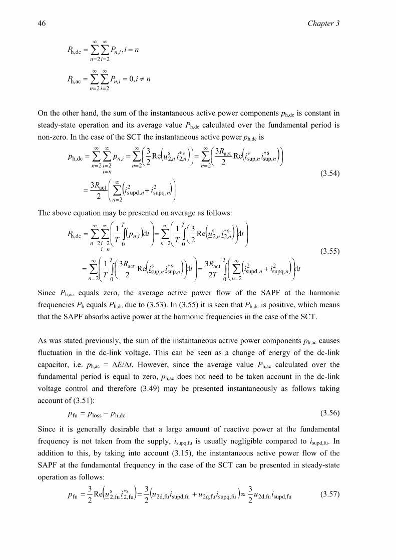
46 Chapter 3
niPPn i
in == ∑∑∞
=
∞
=,
2 2,dch,
niPPn i
in ≠== ∑∑∞
=
∞
=,0
2 2,ach,
On the other hand, the sum of the instantaneous active power components ph,dc is constant in steady-state operation and its average value Ph,dc calculated over the fundamental period is non-zero. In the case of the SCT the instantaneous active power ph,dc is
( ) ( )
( )⎟⎟⎠
⎞⎜⎜⎝
⎛+=
⎟⎠⎞
⎜⎝⎛=⎟
⎠⎞
⎜⎝⎛==
∑
∑∑∑∑
∞
=
∞
=
∞
=
∞
=
∞
==
2
2,supq
2,upds
act
2
s*sup,
sup,s
act
2
s*,2
s,2
2 2,dch,
23
Re2
3Re23
nnn
nnn
nnn
nni
iin
iiR
iiRiupp
(3.54)
The above equation may be presented on average as follows:
( ) ( )
( ) ( )∫ ∑∑ ∫
∑ ∫∑∑ ∫
⎟⎟⎠
⎞⎜⎜⎝
⎛+=
⎟⎟
⎠
⎞
⎜⎜
⎝
⎛⎟⎠⎞
⎜⎝⎛=
⎟⎟
⎠
⎞
⎜⎜
⎝
⎛⎟⎠⎞
⎜⎝⎛=
⎟⎟
⎠
⎞
⎜⎜
⎝
⎛=
∞
=
∞
=
∞
=
∞
=
∞
==
T
nnn
n
T
nn
n
T
nnn
nii
T
in
tiiT
RtiiRT
tiuT
tpT
P
0 2
2supq,
2supd,
act
2 0
s*,sup
sup,s
act
2 0
s*,2
s,2
2 2 0,dch,
d2
3dRe2
31
dRe231d1
(3.55)
Since Ph,ac equals zero, the average active power flow of the SAPF at the harmonic frequencies Ph equals Ph,dc due to (3.53). In (3.55) it is seen that Ph,dc is positive, which means that the SAPF absorbs active power at the harmonic frequencies in the case of the SCT. As was stated previously, the sum of the instantaneous active power components ph,ac causes fluctuation in the dc-link voltage. This can be seen as a change of energy of the dc-link capacitor, i.e. ph,ac = ΔE/Δt. However, since the average value Ph,ac calculated over the fundamental period is equal to zero, ph,ac does not need to be taken account in the dc-link voltage control and therefore (3.49) may be presented instantaneously as follows taking account of (3.51): h,dclossfu ppp −= (3.56)
Since it is generally desirable that a large amount of reactive power at the fundamental frequency is not taken from the supply, isupq,fu is usually negligible compared to isupd,fu. In addition to this, by taking into account (3.15), the instantaneous active power flow of the SAPF at the fundamental frequency in the case of the SCT can be presented in steady-state operation as follows:
( ) ( ) fusupd,fu2d,fusupq,fu2q,fusupd,fu2d,s*fu,2
sfu,2fu 2
323Re
23 iuiuiuiup ≈+== (3.57)

Operating principles of SAPF based power filters 47
The voltage components that are needed to gain active power flow pfu can now be calculated from the above equation by taking (3.31) and (3.56) into account. Based on these the output voltage vector components of the inverter can be calculated.
( )
⎥⎥⎥
⎦
⎤
⎢⎢⎢
⎣
⎡ −
⎥⎦
⎤⎢⎣
⎡
−=⎥
⎦
⎤⎢⎣
⎡
03
2
3333
6 fusupd,
dch,loss
2
1
fusfq,
fusfd,i
pp
NN
uu
, (3.58)
where ph,dc is achieved using (3.54). In conclusion, to provide current harmonics filtering the SAPF has to generate output voltage at the harmonic frequencies, as defined in (3.32). In addition to this, to maintain constant dc-link voltage also the fundamental voltage component defined in (3.58) has to be produced. Thus the space vector components of the APF output voltage reference are in the case of the SCT:
( )
⎥⎥⎥⎥⎥
⎦
⎤
⎢⎢⎢⎢⎢
⎣
⎡+
−
⎥⎦
⎤⎢⎣
⎡
−=⎥
⎦
⎤⎢⎣
⎡
∑
∑∞
=
∞
=
2supq,act
2supd,act
fusupd,
dch,loss
2
1
sfrefq
sfrefd 32
3333
6
nn
nn
iR
iRi
pp
NN
uu
, (3.59)
where ph,dc is defined in (3.54). In this result it is assumed that the APF does not produce any dc-signals in order to control the dc-currents as was mentioned in Section 3.4.1. The influence of the dc-link voltage control on the filtering performance of the SCT can now be seen in (3.59). As is seen, when the dc-link voltage is maintained using the dc-link voltage control, the output voltage reference includes a fundamental component, which is influenced by losses of the SAPF ploss, active power flow at harmonic frequencies ph,dc, d-component of the supply current at fundamental frequency isupd,fu and transformation ratio of the coupling transformer N1/N2. On the other hand, when the dc-link voltage is maintained using an auxiliary power source this voltage reference component is equal to zero. Because of this, the maximum value of the active resistance Ract, which is possible to reach using the same modulation index, is smaller where the dc-link voltage is maintained using the dc-link voltage control compared to where it is maintained using an auxiliary power source.
3.5 Filter connected topology
The second SHAPF topology examined, which is called filter connected topology (FCT) is presented in Fig. 3.11 (Akagi, 1996; Fujita and Akagi, 1991).

48 Chapter 3
Lco Llo
Load
isup
isf
ilo
Rlo
if
usf
udc
u2
C7
L7
Chp
RhpLhp
Csf
Lsf
Cdc
APF
SupplyC5
usup Lsup
L5
Fig. 3.11. Main circuit of the FCT.
Like the SCT, the FCT consists of the SAPF, two LC shunt circuits and high-pass filter. In the case of the FCT, however, the SAPF is connected in series with the passive filters. The tuning frequencies of the LC shunt circuits are 250 Hz, 350 Hz and 550 Hz (high pass). The essential difference between the SCT and the FCT is that in the FCT less current flows through the coupling transformer and the switching components at the fundamental frequency. Therefore the current rating of the APF is lower in the case of the FCT compared to the SCT (Fujita and Akagi, 1991). The operating principle of the FCT is similar to that of the SCT. The purpose when, using the SAPF, is to produce a voltage that is proportional to the supply current harmonics, as was presented in (3.30). This has the same effect as applying active resistance Ract in the supply branch. In this case, too, the function of the passive filters is to guarantee an alternative path for the load current harmonics instead of the supply, whereas a function of the SAPF is to boost the performance of the passive filters (Rivas et. al, 2003). Although the connection point of the SAPF in the main circuit is different in the case of the FCT than the SCT, the functioning of these SHAPFs is the same, as will be shown. The operating principle of the FCT is next examined using the single-phase equivalent circuits and RMS phasor presentation. The single-phase equivalent circuits of the system at the fundamental frequency and at the harmonic frequencies are shown in Fig. 3.12. The load is presented by using the Norton equivalent circuit and the impedance of three parallel connected passive filters is presented by single impedance Zf.

Operating principles of SAPF based power filters 49
a)
U sup,fuI f,fu
Zsup,fu
I sup,fuZf,fu
Z lo,fuI loi,fu I los,fu
-
+
I lo,fu
b)
U sup,n
U2,n
I f,n
Zsup,n
I sup,nZf,n
Zlo,nI loi,n I los,n
+
- +
-
I lo,n
Fig. 3.12. Single-phase equivalent circuits of the FCT: a) equivalent circuit at the fundamental frequency and b) equivalent circuit at the harmonic frequencies.
If the fundamental frequency component produced by the APF dc-link voltage controller is assumed to be insignificant, the SAPF does not have any influence on the fundamental frequency behaviour of the system, as is shown in Fig. 3.12a. As was the case with the SCT, the load impedance Zlo is next assumed to be very high, i.e. Iloi ≈ 0. The following phasor equation can be generated based on the single-phase equivalent circuit presented in Fig. 3.12b.
nn
nnnnn ZZ
IZUUI
f,sup,
los,f,,2sup,sup, +
+−= (3.60)
Since the control principle of the FCT is similar to that of the SCT, using (3.34) and (3.60) we have
( )
( )( ) n
nn
n
nnn
nn
nnnn
IXXRRR
XR
UXXRRR
RZZIZU
I
,los,fsup,actfsup
,ff
sup,,fsup,actfsup
actf,sup,
los,f,sup,sup,
j
j
j
1
++++
++
++++=
++
+=
(3.61)
It is noticed that (3.61) is the same as (3.45). Because of this the active resistance Ract has in this case the same effect as with the SCT, i.e. the harmonic components of the supply current can be decreased by increasing the active resistance Ract. The simplification Iloi ≈ 0 made in the beginning of the calculation has no influence on this conclusion because if the load impedance Zlo were low, the total impedance of the parallel connected passive filters Zf and load impedance Zlo would be lower than Zf and the SHAPF would operate more effectively.
3.5.1 Control system
The control system of the FCT used in this thesis is presented in Fig. 3.13. It is based on space vector calculation in the synchronous reference frame. The control system is based on the control system presented in (Fujita and Akagi, 1991). However, similar changes to the control system have been made by the author as in the case of the control system of the SCT. In the

50 Chapter 3
control system presented in (Fujita and Akagi, 1991) the harmonics are extracted from the measured supply current using instantaneous power theory. In the control system presented in Fig. 3.13 the extraction of the harmonics is based on high-pass filtering of the supply current space vector in the synchronous reference frame. In addition to this, the control system is improved by adding an additional calculation branch, which is the uppermost calculation branch in Fig. 3.13. The functioning of the branch was explained in the case of the control system of the SCT. The multiplication of the output voltage reference by the matrix M has also been added by the author.
d
Pudc
udcref
+-
Ract
q
a
bisupABC
isfA
isfB
isfC
a
b
+
LPFLPFLPF
HPF
HPF+ +
++
PPP-
+-
+-
+
0 0 0
ab
ABC ab
dq
ab
dqab
ABC
ffu
ffu
usfrefd,dc
usfrefq,dc
usfrefq,h
usfrefd,h
usfrefq,fu
PLLusupA ffu
ussfrefM
Ract
Fig. 3.13. Control system of the FCT.
Because of the similar functioning principles of the SCT and the FCT, their control systems are nearly identical. The control system of the FCT also consists of three calculation branches, which are similar to the calculation branches of the control system of the SCT presented in Fig. 3.10. The only difference between the control systems of the SCT and the FCT can be found in the lowest calculation branch. With the FCT the output signal of the dc-link voltage controller is added only to the q-component of the output voltage reference. This is because the fundamental frequency components of the currents of the passive filters are capacitive and thus leading 90° supply voltage.
3.5.2. Influence of dc-link voltage control on the filtering performance
The influence of dc-link voltage control on current harmonics filtering performance of the SAPF is quite similar in the cases of the FCT and SCT. Because of the similar SAPFs and similar operating principles of the control systems, (3.46) and (3.47) also apply in the case of the FCT. Therefore, also in the case of the FCT higher dc-link voltage enables a better current harmonics filtering performance, because in this case higher active resistance Ract may be applied.

Operating principles of SAPF based power filters 51
Similarly, because of the identical SAPFs, the starting point of the inspection of the influence of the dc-link voltage control on the current harmonics filtering performance of the SAPF is the same. This means that (3.48), (3.49) and (3.56), which describe the average and instantaneous active power flows of the SAPF are valid also in the case of the FCT. However, differences between the topologies arise when the active power flow between the SAPF and the system, where it is connected, are inspected. With the FCT, the coupling transformer is connected in series with the passive filters. The current flowing through the secondary windings of the coupling transformer is the total current of the passive filters, i.e. i2 = if. Because of this, (3.50), which presented the instantaneous active power components pn,i of the SAPF at the harmonic frequencies in the case of the SCT is presented in the case of the FCT as follows:
( ) ( )s*f,
ssup,
acts*,2
s,2, Re
23Re
23
ininin iiRiup == (3.62)
pn,i can be again divided into components ph,dc and ph,ac as was defined in (3.51). ph,dc is calculated as
( ) ( )
( )⎟⎟⎠
⎞⎜⎜⎝
⎛+=
⎟⎠⎞
⎜⎝⎛=⎟
⎠⎞
⎜⎝⎛==
∑
∑∑∑∑
∞
=
∞
=
∞
=
∞
=
∞
==
2fq,supq,fd,supd,
act
2
s*f,
sup,s
act
2
s*,2
s,2
2 2,dch,
23
Re2
3Re23
nnnnn
nnn
nnn
nni
iin
iiiiR
iiRiupp
. (3.63)
The average value Ph,dc can be calculated as
( ) ( )
( )
( )∫ ∑
∑ ∫
∑ ∫∑∑ ∫
⎟⎟⎠
⎞⎜⎜⎝
⎛+=
⎟⎟
⎠
⎞
⎜⎜
⎝
⎛⎟⎠⎞
⎜⎝⎛=
⎟⎟
⎠
⎞
⎜⎜
⎝
⎛⎟⎠⎞
⎜⎝⎛=
⎟⎟
⎠
⎞
⎜⎜
⎝
⎛=
∞
=
∞
=
∞
=
∞
=
∞
==
T
nnnnn
n
T
nn
n
T
nnn
nii
T
in
tiiiiT
R
tiiRT
tiuT
tpT
P
0 2fq,supq,fd,supd,
act
2 0
s*f,
sup,s
act
2 0
s*,2
s,2
2 2 0,dch,
d2
3
dRe2
31
dRe231d1
(3.64)
As was stated already in Section 3.4.2, the average value Ph,ac equals zero. Because of this, the average active power flow of the SAPF at the harmonic frequencies Ph equals Ph,dc calculated in (3.64) due to (3.53). As was mentioned in the case of the SCT, ph,dc has an influence on the dc-link voltage control. However, the direction of the active power flow of the SAPF at the harmonic frequencies in the case of the FCT is not as obvious as it is in the case of the SCT. In (3.63) it is seen that the direction of the active power flow at the harmonic frequencies depends on the phase angle between the supply current vector and the vector of total current of the passive filters. Let us now inspect the division of the load current harmonics between the supply branch and the

52 Chapter 3
total current of the passive filter branches. Based on the equivalent circuit shown in Fig. 3.12b and on (3.34) the transfer function from the total current of the passive filters to the supply current is presented at harmonic frequencies as
( ) ( )( )
( )( )
( ) ( ) ( )( )( ) ( ) ( ) ( ) ( ) ( ) ( )( )sZsZsZsZsZsZRsZ
sZsZsZ
RssZ
sIsI
sG
nnnnnnn
nnn
n
n
n
n
,hp,5,hp,7,7,5actup,s
hp,7,5,
actsup,
f,
f,
sup,
Z
+++−=
+−==
(3.65)
where ( ) supdcsupsup, RsLsZ n +=
is the supply impedance and
( )sC
sCRsCLsZ n5
55dc2
55,5
1++=
( )sC
sCRsCLsZ n7
77dc2
77,7
1++=
( ) ( )( ) sCRRsCL
RRsLRRCsRCLsZ n
hphpdchp2
hphp
hpdchphphpdchphp2
hphphp,hp
++
++++=
are the impedances of the LC shunt circuits and the high-pass filter. In these equations, the series dc-resistances of the inductors (Rsupdc, R5dc, R7dc and Rhpdc) are taken account as non-idealities. Although (3.65) was based on the equivalent circuit presented at harmonic frequencies, it also applies at the fundamental frequency if it is noticed that in this case Ract equals zero. The frequency response of the transfer function G(s) is presented in Fig. 3.14 using the component values presented in Table C.2 in Appendix C.
Fig. 3.14. Frequency response from the total current of the passive filters to the supply current, Ract = 0 Ω (-), Ract = 5 Ω (--) and Ract = 10 Ω (.-).

Operating principles of SAPF based power filters 53
In the above figure it is seen that the supply current and the total current of the passive filters are in the different phase at 250 Hz and 350 Hz, which are usually the highest harmonics in the system. Their phase difference at frequencies higher than 500 Hz is nearly 90°. Fig. 3.14 presents the frequency response of the real passive filters, where the resonance frequency is designed to be slightly lower than the harmonic frequency that is to be filtered in order to prevent overloading. Theoretically, if the resonance frequencies of the passive filters were exactly the same as the harmonic frequencies that are to be filtered, the phase difference between the supply current and the total current of the passive filters would be 90° at these frequencies. Therefore, based on (3.63) the active power flow of the SAPF is negligible at the harmonic frequencies in the case of the FCT, i.e. ph,dc ≈ 0. In practice this means that in the case of the FCT only a small amount of energy is changed between the SAPF and the main circuit at harmonic frequencies. The d-component of the total current of the passive filters at the fundamental frequency ifd,fu is negligible compared to the q-component ifq,fu in the supply voltage oriented synchronous reference frame. This is because the currents of the passive filters are capacitive at the fundamental frequency and thus leading the supply voltage 90°. The instantaneous active power of the FCT at the fundamental frequency in steady-state operation is in this case:
( ) ( ) fufq,fu2q,fufq,fu2q,fufd,fu2d,s*fu,2
sfu,2fu 2
323Re
23 iuiuiuiup ≈+== (3.66)
The voltage components that are needed to gain active power flow pfu can now be calculated from the above equation by taking (3.31) and (3.56) into account. In addition to this, it must be noticed that ph,dc ≈ 0 as was earlier stated. Based on this, the following equation is achieved.
⎥⎥
⎦
⎤
⎢⎢
⎣
⎡⎥⎦
⎤⎢⎣
⎡
−=⎥
⎦
⎤⎢⎣
⎡
fufq,
loss2
1
fusfq,
fusfd,
32
0
3333
6 ip
NN
uu
(3.67)
In the case of the FCT the output voltage of the APF also consists of the voltage components at the harmonic frequencies to provide current harmonics filtering and the fundamental voltage component used for the dc-link voltage control. These were defined in (3.32) and (3.67). Based on these, the space vector components of the APF output voltage reference are in the case of the FCT:
⎥⎥⎥⎥⎥
⎦
⎤
⎢⎢⎢⎢⎢
⎣
⎡
+⎥⎦
⎤⎢⎣
⎡
−=⎥
⎦
⎤⎢⎣
⎡
∑
∑∞
=
∞
=
2supq,act
fufq,
loss
2supd,act
2
1
sfrefq
sfrefd
3233
336
nn
nn
iRip
iR
NN
uu
. (3.68)
In this result it is assumed that the inverter does not produce any dc-signals in order to control the dc-currents, as was mentioned in Section 3.4.1.

54 Chapter 3
The influence of the dc-link voltage control on the filtering performance of the FCT is seen in (3.68). Similarly as with the SCT, the maximal value of the active resistance Ract has to be smaller in this case than where dc-link voltage is maintained using an auxiliary power supply if the same modulation index is used. This is because of the fundamental voltage component, which is influenced by the losses of the SAPF ploss, q-component of the passive filter currents at the fundamental frequency ifq,fu and the transformation ratio of the coupling transformer N1/N2. By comparing equations (3.59) and (3.68) it is noticed that in the case of the FCT the output voltage reference at the fundamental frequency is not decreased by the active power flow at the harmonic frequencies ph,dc as is the case with the SCT. Because of this, larger output voltage at the fundamental frequency has to be produced with the FCT than with the SCT in order to gain the same active power flow. It is also noticed that in the case of the FCT the output voltage at the fundamental frequency is inversely proportional to the q-component of the passive filter currents ifq,fu, and in the case of the SCT it is inversely proportional to the d-component of the supply current isupd,fu. Since isupd,fu is always higher than ifq,fu, the amplitude of the output voltage at the fundamental frequency has to be higher with the FCT than with the SCT in order to gain the same active power flow. In conclusion, because of these two reasons the maximal value of the active resistance Ract has to be smaller in the case of the FCT if the same modulation index is used. Because of this the dc-link voltage control has a larger influence on the filtering performance of the FCT than that of the SCT.
3.6 Electrically tuned LC shunt circuit
Fig. 3.15 shows the third SHAPF topology, which is called electrically tuned LC-filter (ETLC) (Bhattacharya et. al., 1997).
Lsup
Csf
Lsf
Cdc
APF
Supply
Lf
Cf
Lco
Load
isup
isf
if
udc
usf
Rlo
Lloilo
u2
Fig. 3.15. Main circuit of the ETLC.

Operating principles of SAPF based power filters 55
The main circuit of the ETLC consists of the SAPF and the LC shunt circuit connected in parallel with the load. The SAPF is connected in series with the LC shunt circuit. The resonance frequency of the LC shunt circuit is not tuned for any precise frequency since it is tuned electrically using the SAPF. The benefit of the ETLC is that the VA-rating of the inverter can be designed low, because only a small current flows through it (Bhattacharya et. al., 1997). The functioning principle of the ETLC is to form a low impedance path for the harmonic components of the load current. Just as with the two previous topologies, when the impedance of the LC shunt circuit seen from the load by the harmonic current components is smaller than the impedance of the supply, the harmonic components of the load current will flow into the LC shunt circuit rather than into the supply. With the ETLC, the purpose of the SAPF is to tune the resonance frequency of the LC shunt circuit electrically for the individual harmonic components. This is done by generating so-called active inductance Lact into the system by the SAPF at these frequencies. The resonance frequency of the LC shunt circuit fr can be tuned by controlling this active inductance at each harmonic frequency:
( )nn
LLCf
,actffr, π2
1+
= , (3.69)
where Cf and Lf are the capacitance and inductance of the LC shunt circuit. The general idea of generating this kind of virtual impedance using power electronic switches has been originally presented by Divan (1984). Later, a similar idea, which was named “variable active-passive reactance (VAPAR)”, was also proposed, analysed and tested by Funato and Kawamura (1992 and 1993). The generation of active inductances is done as follows. The active inductances Lact,n are realised by creating the output voltage usf using the SAPF. The required space vector of the output voltage is calculated based on the inductor voltage equation in the rotating reference frame. The space vector presentation of the nth harmonic component of the compensation voltage seen on the secondary side of the coupling transformer presented in the harmonic reference frame, whose angular speed corresponds to nth harmonic frequency component, is
nnnn
nnn
nn
nn
n iLii
Lu f,act,f,f,
act,,2 jjdt
dωω =
⎟⎟
⎠
⎞
⎜⎜
⎝
⎛+= , (3.70)
where if is the LC shunt circuit current. In the above equation dinf,n/dt equals zero in the steady
state situation, because the nth harmonic component of the passive filter current vector in
f,n is a dc-quantity in the reference frame rotating at angular speed corresponding to the nth
harmonic frequency.

56 Chapter 3
The output voltage vector usf may consist of several frequency components usf,n, which means that the active inductance Lact can be applied simultaneously at several frequencies and its value at each frequency can be chosen individually (Bhattacharya et. al., 1997). The resulting output voltage us
sf is a sum of the voltage components unsf,n, which are transformed to the
supply voltage oriented synchronous reference frame. The space vector components of the output voltage usf may be calculated using (3.14), (3.31) and (3.70):
( )( ) ( )( )( )( ) ( )( )
( )( ) ( )( )( )( ) ( )( )∑
∑
=
=
⎟⎟
⎠
⎞
⎜⎜
⎝
⎛
⎥⎥⎦
⎤
⎢⎢⎣
⎡−⎥⎦
⎤⎢⎣
⎡−−−−−
=
⎟⎟
⎠
⎞
⎜⎜
⎝
⎛
⎥⎥⎦
⎤
⎢⎢⎣
⎡⎥⎦
⎤⎢⎣
⎡−−−−−
=
⎥⎦
⎤⎢⎣
⎡=⎥
⎦
⎤⎢⎣
⎡
ii
inn
nnn
nnnn
nn
nn
ii
inn
n
nn
nn
nn
iLiL
tttt
uu
tttt
uu
uu
fd,act,
fq,act,
ss
ss
,2q
,2d
ss
ss
2q
2d
sfq
sfd
cossinsincos
)71.3(cossinsincos
ωω
ωωωωωωωω
ωωωωωωωω
M
M
M
where n = i,ii are the harmonic frequency components, where the active inductance Lact,n is applied. In this work, n = 5,7. The functioning principle of the ETLC is next examined using single-phase equivalent circuits and RMS phasor presentation. The single-phase equivalent circuits of the system at the fundamental frequency and at the harmonic frequencies are shown in Fig. 3.16. The load is presented by using the Norton equivalent circuit and the load impedance Zlo is assumed to be very high, i.e. Iloi ≈ 0.
a)
U sup,fuI f,fu
Zsup,fu
I sup,fuZf,fu
Zlo,fuI loi,fu I los,fu
-
+
I lo,fu
b)
U sup,n
U2,n
I f,n
Zsup,n
I sup,nZf,n
Zlo,nI loi,n I los,n
+
- +
-
I lo,n
Fig. 3.16. Single-phase equivalent circuits of the ETLC: a) equivalent circuit at the fundamental frequency and b) equivalent circuit at the harmonic frequencies.
If the fundamental frequency component produced by the APF dc-link voltage controller is assumed to be insignificant, the SAPF does not have any influence on the fundamental frequency behaviour of the system as is shown in Fig. 3.16a. Based on Fig. 3.16b, the following steady-state phasor presentation of the ETLC can be written:
nn
nnnnn ZZ
IZUUI
f,sup,
los,f,2,sup,sup, +
+−= (3.72)
The RMS phasor presentation of (3.70) is

Operating principles of SAPF based power filters 57
nnn IXU f,act,2, j= (3.73)
Now, since If,n = Isup,n – Ilos,n, substituting the above equation into (3.72) yields
( )( )( ) n
nnn
nn
nnnn
nnn
nnnnnn
IXXXRR
XXR
UXXXRR
XZZIXIZU
I
los,act,f,sup,fsup
act,f,f
sup,act,f,sup,fsup
act,f,sup,
los,act,los,f,sup,sup,
jj
j1
jj
++++
+++
++++=
++
++=
(3.74)
In the above equation it is seen that if the reactance of the active inductance Xact,n is chosen to be equal to but of the opposite sign than the reactance of the LC shunt circuit Xf,n, the harmonic components of the supply current Isup,n are decreased. It is seen that in this case the filtering characteristics of the ETLC depend on the ratio of the LC shunt circuit resistance Rf and the supply impedance Rsup + jXsup,n. Besides applying the active inductances Lact,n, the active resistance Ract can also be simultaneously generated. In this case, by combining (3.34) and (3.73) we have nnnn IRIXU sup,actf,act,2, j += (3.75)
Substituting this into (3.72) and noticing that If,n = Isup,n – Ilos,n we have
( )( )( ) n
nnn
nn
nnnn
nnn
nnnnnn
IXXXRRR
XXR
UXXXRRR
XRZZIXIZU
I
los,act,f,sup,actfsup
act,f,f
sup,act,f,sup,actfsup
act,actf,sup,
los,act,los,f,sup,sup,
jj
j1
jj
+++++
+++
+++++=
+++
++=
(3.76)
In the above equation it is seen that due to the active resistance Ract, the harmonic components of the supply current Isup,n are further decreased compared to the case presented in (3.74), where only active inductances Lact,n were applied.
3.6.1. Control system
The control system of the ETLC is presented in Fig. 3.17. The control system is based on space vector calculation in the supply voltage oriented synchronous reference frame. The control system is presented in (Bhattacharya et. al., 1997). The control system is improved by the author in a similar way to the control systems of the previous topologies. An additional calculation branch, which is the uppermost calculation branch in Fig. 3.17, has been added to the control system. The purpose of the control branch is to remove the dc-levels of the primary side (inverter side) phase currents of the coupling transformer. Its functioning was explained in the case of the control system of the SCT. The multiplication of the output

58 Chapter 3
voltage reference by the matrix M has also been added by the author. The purpose of the multiplication is to take the delta connection of the primary side of the coupling transformer into account.
d,5
q,5
a
bifABC
LPF
LPF
K5
-K5
d,7
q,7
LPF
LPF
K7
-K7
Pudc
udcref
+-
+ +
+
++
+
isfA
isfB
isfC
a
b
LPFLPFLPF
+
-
+-
+-
+
0 0 0
ab
ABC
ab
ABC
ab
d5q5
ab
d7q7
ab
dq
dq
d5q5
dq
d7q7
ffu
ffu
ffu
f5
f7
usfrefd,dc
usfrefq,dc
usfrefd,5
usfrefq,5
usfrefd,7
usfrefq,7
usfrefq,fu
PLLusupAffuf5f7
ussfrefM
f5
f7
Fig. 3.17. Control system of the ETLC.
The active inductances Lact,n are calculated in two calculation branches in the middle of the control system. In this case the active inductances for the 5th and 7th harmonic frequencies are calculated. The functioning principles of both calculation branches are similar. The phase currents of the LC shunt circuit ifA, ifB and ifC are first transformed into the space vector components in the rotating reference frame. The rotating frequency of the frame is the same as the harmonic frequency that is to be filtered. These signals are low-pass filtered to obtain the nth harmonic of the original signal, which is a dc-quantity in the given reference frame in steady-state operation. After this, the signals are multiplied by the coefficient Kn and interchanged. The coefficient Kn is calculated based on (3.70) by solving the quadratic components of the presented space vector and by noticing that din
f,n/dt is equal to zero.
⎥⎥⎦
⎤
⎢⎢⎣
⎡−=
⎥⎥⎦
⎤
⎢⎢⎣
⎡−=
⎥⎥⎦
⎤
⎢⎢⎣
⎡n
n
nn
nnn
nn
nnnn
nn
ii
Kii
Luu
fd,
fq,
fd,
fq,,act
,q2
d,2 ω , (3.77)
where Kn = Lact,nωn. After this, the resulting space vector is transformed to the supply voltage oriented synchronous reference frame and the resulting voltage reference vector us
sfref,n is summed to the outputs of other calculation branches. The lowest and the uppermost branches, which are used for dc-link voltage control and to control the APF output current dc-levels, are similar to the control systems of the SCT and the

Operating principles of SAPF based power filters 59
FCT and thus their functioning is not presented here. The APF output voltage reference vector us
sfref is finally achieved by summing the outputs of all calculation branches and multiplying the result by the matrix M. The control system of the ETLC, where also the control of the active resistance Ract is included, is presented in Fig. 3.18. The idea of this control system, where the controls of the active resistance Ract and the active inductances Lact are combined, is proposed by the author. The control system is otherwise similar to the previous one, but in this case the branch that controls the active resistance Ract is added. As is seen, the calculation branch is identical to the one which was used for the active resistance control in the cases of the SCT and the FCT and thus its functioning is not presented here. The voltage reference produced by this branch is added to the outputs of other calculation branches.
d,5
q,5
a
bifABC
LPF
LPF
K5
-K5
d,7
q,7
LPF
LPF
K7
-K7
+
isfA
isfB
isfC
a
b
LPFLPFLPF -
+-
+-
+
0 0 0
ab
ABC
ab
ABC
ab
d5q5
ab
d7q7
ab
dq
dq
d5q5
dq
d7q7
dRact
q
a
bisupABC
HPF
HPF
ab
dqab
ABC
Pudc
udcref
+-
+
+
++
+
+ +
+
ffu
ffu
ffu
ffu
f5
f7
usfrefd,dc
usfrefq,dc
usfrefd,5
usfrefq,5
usfrefd,7
usfrefq,7
usfrefd,h
usfrefq,h
usfrefq,fu
PLLusupAffuf5f7
Ract
ussfrefM
f5
f7
Fig. 3.18. Control system of the ETLC with combined control of the active resistance and the active inductances.

60 Chapter 3
3.7 UPQC
The main circuit of the unified power quality conditioner (UPQC) examined in this work is presented in Fig. 3.19 (Akagi, 1996; Emadi et. al., 2005; Turunen and Tuusa, 2006; Turunen and Tuusa, 2007). The main circuit of the UPQC consists of two APFs: the SAPF and parallel active power filter (PAPF). The SAPF is connected in series with the supply and the PAPF is connected in parallel with the load. The high frequency ripple caused by the inverter action is filtered in the case of the SAPF using LC-filter and in the case of the PAPF using the LCL-filter. The inverters of the APFs are back-to-back connected, i.e. they have a common dc-link. The operating principle of the UPQC is twofold. The purpose of the SAPF is to improve the quality of the load voltage by injecting the compensation voltage u2, whose amplitude is equal and phase opposite to the distortions of the supply voltage usup, as was presented in (3.39).
Csf
Lsf
Cdc
SAPF
usup
Supply
Lco
Load
isup
isf
ilo
Rlo
Llo
udc
usf
PAPF
LpfipfCpf
Lpm
upf
ulo
Rpm
u2
ipm
Fig. 3.19. Main circuit of the UPQC.
On the other hand, the purpose of the PAPF is to improve the quality of the supply current by injecting the compensation current ipm. At the harmonic frequencies, the amplitude of ipm is equal and the phase opposite to the harmonic components of the load current ilo. In addition to this, the PAPF is used to compensate for the reactive power taken by the load. Therefore, the vector components of the compensation current reference ipmref in the supply voltage oriented synchronous reference frame are:
( )
( )⎥⎥⎥⎥⎥
⎦
⎤
⎢⎢⎢⎢⎢
⎣
⎡
−+−
−=⎥
⎦
⎤⎢⎣
⎡
∑
∑∞
=
∞
=
2loq,fuloq,
2lod,
pmrefq
pmrefd
nn
nn
ii
i
ii
. (3.78)

Operating principles of SAPF based power filters 61
The compensation current ipm also includes the real component at the fundamental frequency in the synchronous reference frame since the PAPF takes care of the control of the dc-link voltage. However, this is ignored in (3.78). The single-phase equivalent circuits of the system shown in Fig. 3.19 are presented at the fundamental frequency and at the harmonic frequencies in Fig. 3.20. The load is presented by using the Norton equivalent circuit.
a)
I los,fuU sup,fu
Zsup,fuU2,fu
I sup,fu
I loi,fu Zlo,fu
+
-
+ -
I pm,fu
U lo,fuI lo,fu
b)
I los,nU sup,n
Zsup,nU2,n
I sup,n
I loi,n Zlo,n
+
-
+ -
Ipm,n
U lo,nI lo,n
Fig. 3.20. Single-phase equivalent circuits of the UPQC: a) equivalent circuit at the fundamental frequency and b) equivalent circuit at the harmonic frequencies.
The functioning of the system may be analysed based on the equivalent circuits. The functioning of the SAPF is similar to the functioning of the pure SAPF, which was analysed in Chapter 3.3 using (3.40) – (3.43). The functioning of the PAPF is as follows. At the fundamental frequency the purpose of the PAPF is to compensate the reactive power. If the angle of the load voltage phasor is ϕulo,fu at the fundamental frequency and the angle of the load current phasor ϕilo,fu, the phasor of the compensation current generated by the PAPF at the fundamental frequency is
( ) ( )°±∠−= 90sin fuulo,fuilo,fuulo,fulo,fupm, ϕϕϕII . (3.79)
The sign of the phase angle of 90° added to the phase angle of the compensation current depends on whether the reactive power is produced or taken by the load. Now, if it assumed that the load impedance is high, i.e. Iloi ≈ 0, the following phasor equation can be written based on Fig. 3.20a. fulos,fupm,fusup, III += (3.80)
If now (3.79) is substituted into (3.80), it results in Isup,fu = |Ilos,fu|cos(ϕulo,fu - ϕilo,fu)∠ϕulo,fu, i.e. only active power is transferred from the supply to the load. In addition to reactive power compensation, the real fundamental frequency component is also generated by the PAPF because of the dc-link voltage controller. However, in this examination the voltage component caused by the dc-link controller was treated as negligible. At the harmonic frequencies the purpose of the PAPF is to filter supply current harmonics. Therefore at the harmonic frequencies the output current is presented as nn II lo,pm, −= (3.81)
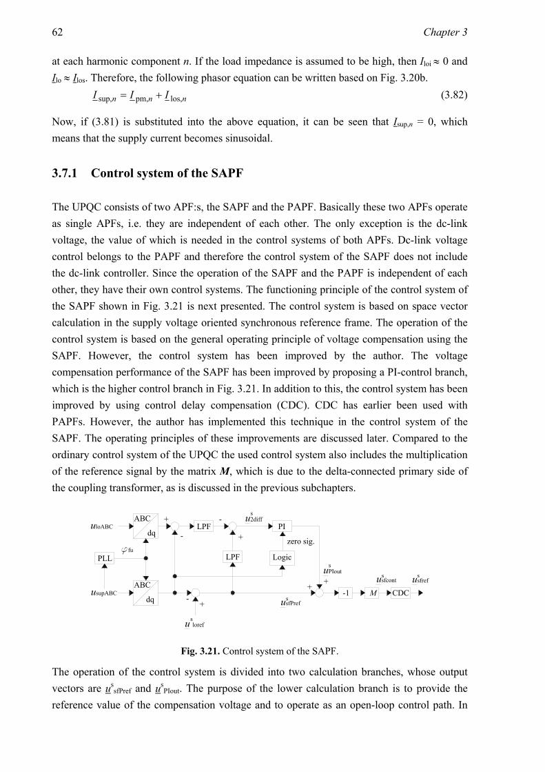
62 Chapter 3
at each harmonic component n. If the load impedance is assumed to be high, then Iloi ≈ 0 and Ilo ≈ Ilos. Therefore, the following phasor equation can be written based on Fig. 3.20b. nnn III los,pm,sup, += (3.82)
Now, if (3.81) is substituted into the above equation, it can be seen that Isup,n = 0, which means that the supply current becomes sinusoidal.
3.7.1 Control system of the SAPF
The UPQC consists of two APF:s, the SAPF and the PAPF. Basically these two APFs operate as single APFs, i.e. they are independent of each other. The only exception is the dc-link voltage, the value of which is needed in the control systems of both APFs. Dc-link voltage control belongs to the PAPF and therefore the control system of the SAPF does not include the dc-link controller. Since the operation of the SAPF and the PAPF is independent of each other, they have their own control systems. The functioning principle of the control system of the SAPF shown in Fig. 3.21 is next presented. The control system is based on space vector calculation in the supply voltage oriented synchronous reference frame. The operation of the control system is based on the general operating principle of voltage compensation using the SAPF. However, the control system has been improved by the author. The voltage compensation performance of the SAPF has been improved by proposing a PI-control branch, which is the higher control branch in Fig. 3.21. In addition to this, the control system has been improved by using control delay compensation (CDC). CDC has earlier been used with PAPFs. However, the author has implemented this technique in the control system of the SAPF. The operating principles of these improvements are discussed later. Compared to the ordinary control system of the UPQC the used control system also includes the multiplication of the reference signal by the matrix M, which is due to the delta-connected primary side of the coupling transformer, as is discussed in the previous subchapters.
ABC
dqusupABC
u loref
ffu
usfref
PLL
s
uloABCdq
ABCLPF
+
-
-
+
LPF
PIu2diff
zero sig.
Logic
s
++
MusfPref
s
uPIouts
s
-1
usfconts
CDC
Fig. 3.21. Control system of the SAPF.
The operation of the control system is divided into two calculation branches, whose output vectors are us
sfPref and usPIout. The purpose of the lower calculation branch is to provide the
reference value of the compensation voltage and to operate as an open-loop control path. In

Operating principles of SAPF based power filters 63
this calculation branch the supply voltage usup is first measured and its space vector calculated using (3.5) and (3.11). The space vector of usup is first compared to reference value us
loref = 325+j0. This reference value is used since a low-voltage supply with nominal phase voltage of 230 VRMS is assumed. The result of the comparison is the space vector us
sfPref. The phase angle ϕfu of the synchronous reference frame is generated by a phase-locked loop (PLL). The purpose of the higher calculation branch, whose output vector is us
PIout is to enhance the performance of the control system at the fundamental frequency. This is achieved by using the closed-loop control method. In this calculation branch inverse of the space vector of the compensation voltage u2 is first found by calculating the difference of the space vectors of the load and supply voltages ulo and usup. This vector is low-pass filtered (LPF) to obtain the fundamental component of -u2, which is seen as a dc-component in the control system. The reference vector, which is also a dc-component in the given reference frame is achieved by low-pass filtering the voltage reference vector us
sfPref. After this, the difference of these vectors us
2diff is fed into the PI-controller, whose output is the space vector usPIout. The PI-
controller is used only in steady-state. If a dynamic change in the supply voltage is observed by the control block “Logic”, it disables the PI-controller. The “zero signal” resets the output signal us
PIout and also the internal variables of the PI-controller and keeps them at zero as long as the state of the supply voltage is changing. This is implemented by continuously calculating the mean value of the d-component of the supply voltage during the last 10 ms and by comparing the latest d-component value with this mean value. If the difference of these values is higher than the preset value, the state of the system is defined as changing. Finally, the output vectors of these control branches, us
sfPref and usPIout, are summed. After this,
inverse of the sum vector is multiplied by matrix M and fed to the control delay compensator (CDC). The multiplication by coefficient -1 is because of chosen polarity of the transformer. The derivation of matrix M is presented in Appendix A. The idea of the control delay compensator is to decrease the influence of delays of the control system and its operating principle is presented later. The output voltage reference vector of the inverter us
sfref which is fed to the space vector modulator is the output vector of the control delay compensator.
The improvement of the compensation performance using the PI-control
The idea behind the PI-control branch, whose output is usPIout is next explained. If this
calculation branch did not exist, i.e. usPIout = 0, the control method of the control system would
be an open-loop control, where the P-controller is used with gain P = 1. However, the voltage compensation performance of the SAPF is poor at the fundamental frequency if the open-loop control system is used, because in practice it always produces a steady-state error (Dorf and Bishop, 1998). In addition to this, the compensation performance is also decreased by the component tolerances of the SAPF and the dead times of the inverter switches.

64 Chapter 3
However, these errors may be avoided and the steady-state error of the load voltage ulo at the fundamental frequency decreased to zero by using the closed-loop control method with the PI-controller. In the proposed closed loop control system the actual coupling transformer voltage u2 at the fundamental frequency is compared to its reference value. The purpose of the PI-controller is to force the error between these signals to zero, which means that the fundamental frequency component of the compensation voltage u2 exactly follows its reference value. However, it must be noticed that this concerns only the fundamental frequency component since it can be seen as a dc-component in this reference frame and because the PI-controller works properly only when its reference signal is a dc-component. In addition to this, in the case where the system is in dynamic change it is advantageous to disable the PI-controller, since its integrating part makes the response of the control system slower. The PI-control may be enabled again after the dynamic change to ensure a good steady-state performance.
3.7.2 Control system of the PAPF
The operating principle of the control system of the PAPF shown in Fig. 3.22 is next presented. The control system is based on the space vector calculation in the supply voltage oriented synchronous reference frame and is taken from (Routimo, 2002).
iloABC
dq
ABC
ipfd
+ -HPF CDC
CDC
ipfq
PID
PID
+ + ++ +
Pc
Pc
-
-+
Pe2
upfrefdipfrefd
ipfrefq
PLLudc
ipfABC ABC
dq
ffu
ipfd
ipfq
upfrefq
dq
ABCuloABCulod
uloq
ulod
uloq
ffu
ffu
ffu
udcref
Fig. 3.22. Control system of the PAPF.
First, the load current ilo is measured and its space vector in the synchronous reference frame calculated using (3.5) and (3.11). The angle ϕfu of the synchronous reference frame is generated by a phase-locked loop (PLL). Next, the d-component of the load current space vector is high-pass filtered (HPF) and the delays of the control system compensated (CDC). The control delay compensation in the case of voltage source PAPF is presented in (Routimo et. al., 2003). The output signal of the dc-link voltage controller is added to the d-component of the output current reference in order to maintain the constant dc-link voltage. The achieved PAPF current reference components ipfrefd and ipfrefq are compared to the space vector components of the measured PAPF output current ipfd and ipfq and the error signals are fed into

Operating principles of SAPF based power filters 65
the PID-controllers. Next, the cross-coupling terms Pc⋅ipfrefq and -Pc⋅ipfrefd, where Pc = ωs(Lpf+Lpm) are summed to the outputs of the PID-controllers. Finally, the achieved space vector components are subtracted from the load voltage space vector components ulod and uloq. The resulting PAPF output voltage reference vector us
pfref is fed to the space vector modulator. The dc-link controller, which is included in the control system of the PAPF, is based on the proportional error squared (Pe2) controller. The error between the measured dc-link voltage and its reference value is fed into the Pe2-controller, whose output signal is added to the d-component of the PAPF output current reference.
3.7.3 Control delay compensation
The control systems of modern APFs are digital. One drawback of digital controllers is the control delay, i.e. there is a delay between the time instants when the control system measures the needed signals and produces the output signal. Because of this control delay, the filtering performance of the APF is degraded. However, the influence of the control delay on the filtering performance of the APF may be reduced by using control delay compensation (CDC). This method is presented in (Salo, 2002) in the case of the current source PAPF and in (Routimo et. al., 2003) that of the voltage source PAPF. Next is presented how the CDC method is applied to the control system of the SAPF when the SAPF is used to compensate the errors of the supply voltage. In the inspected control system the PI-control method, which was presented in Section 3.7.1, is not used. In addition to this, the primary side of the coupling transformer is assumed to be wye-connected, and therefore the coupling matrix M is not needed in the control system. The operation of the SAPF and its control system in general is presented in Fig. 3.23 in the case where the CDC is not used. The operation is inspected at discrete time instants ti, ti+1, ti+2 etc, which are the time instants when the control algorithm is executed. The time interval between these time instants is called the sampling time Ts.
usupd
uerr
ulorefd
usfrefd
0
uerr
u2d0
u2appd
ti ti+1 ti+2 ti+3 ti+4 ti+5
uerr
Fig. 3.23. Operation of the control system of the SAPF.
In Fig. 3.23, the uppermost curve presents the error appearing in the d-component of the
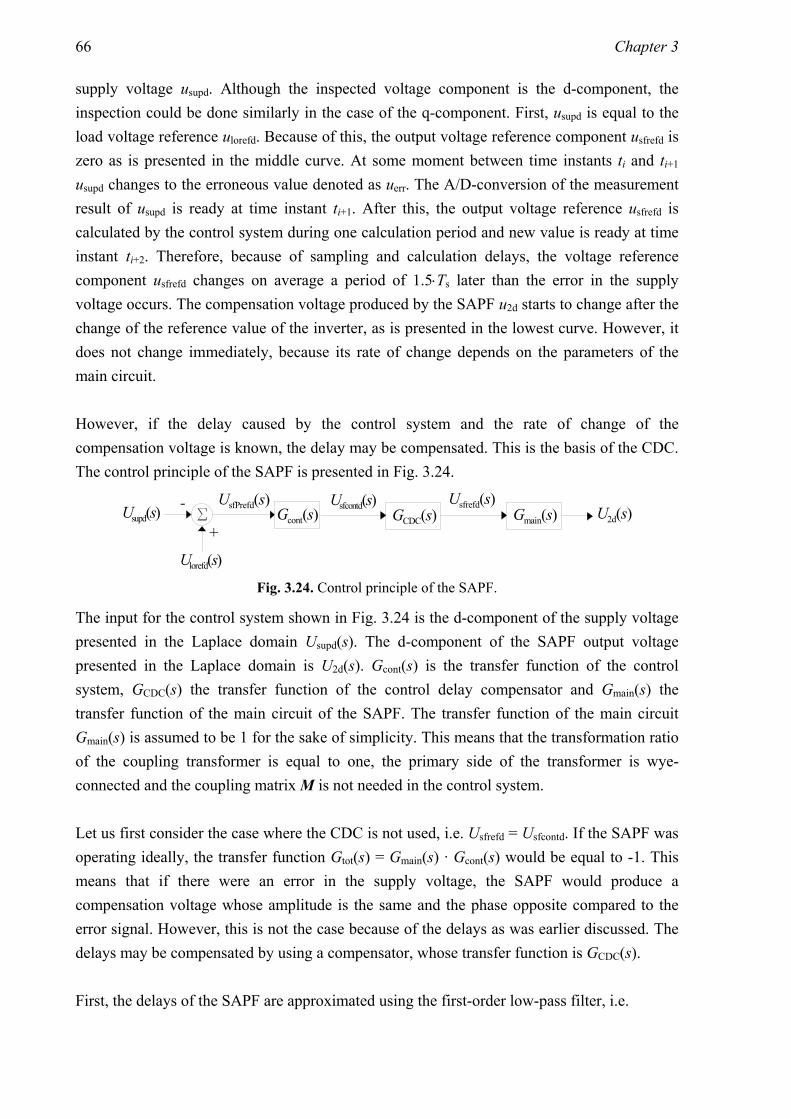
66 Chapter 3
supply voltage usupd. Although the inspected voltage component is the d-component, the inspection could be done similarly in the case of the q-component. First, usupd is equal to the load voltage reference ulorefd. Because of this, the output voltage reference component usfrefd is zero as is presented in the middle curve. At some moment between time instants ti and ti+1 usupd changes to the erroneous value denoted as uerr. The A/D-conversion of the measurement result of usupd is ready at time instant ti+1. After this, the output voltage reference usfrefd is calculated by the control system during one calculation period and new value is ready at time instant ti+2. Therefore, because of sampling and calculation delays, the voltage reference component usfrefd changes on average a period of 1.5⋅Ts later than the error in the supply voltage occurs. The compensation voltage produced by the SAPF u2d starts to change after the change of the reference value of the inverter, as is presented in the lowest curve. However, it does not change immediately, because its rate of change depends on the parameters of the main circuit. However, if the delay caused by the control system and the rate of change of the compensation voltage is known, the delay may be compensated. This is the basis of the CDC. The control principle of the SAPF is presented in Fig. 3.24.
GCDC(s) Gmain(s)Usfcontd(s) U2d(s)Gcont(s)S
+
-Usupd(s)
Ulorefd(s)
Usfrefd(s)UsfPrefd(s)
Fig. 3.24. Control principle of the SAPF.
The input for the control system shown in Fig. 3.24 is the d-component of the supply voltage presented in the Laplace domain Usupd(s). The d-component of the SAPF output voltage presented in the Laplace domain is U2d(s). Gcont(s) is the transfer function of the control system, GCDC(s) the transfer function of the control delay compensator and Gmain(s) the transfer function of the main circuit of the SAPF. The transfer function of the main circuit Gmain(s) is assumed to be 1 for the sake of simplicity. This means that the transformation ratio of the coupling transformer is equal to one, the primary side of the transformer is wye-connected and the coupling matrix M is not needed in the control system. Let us first consider the case where the CDC is not used, i.e. Usfrefd = Usfcontd. If the SAPF was operating ideally, the transfer function Gtot(s) = Gmain(s) · Gcont(s) would be equal to -1. This means that if there were an error in the supply voltage, the SAPF would produce a compensation voltage whose amplitude is the same and the phase opposite compared to the error signal. However, this is not the case because of the delays as was earlier discussed. The delays may be compensated by using a compensator, whose transfer function is GCDC(s). First, the delays of the SAPF are approximated using the first-order low-pass filter, i.e.

Operating principles of SAPF based power filters 67
( ) ( ) ( )sUs
sUsU sfPrefd2appd2d 11+
−=≈τ
, (3.83)
where the time constantτ depends on the control delay and the parameters of the main circuit. In this work, τ = Ts is used. The time domain presentation of the approximated inverter output voltage vector component u2appd is presented as the lowest curve in Fig. 3.23. Based on (3.83) the transfer function Gtot(s) is in the case where the CDC is not used:
( ) ( ) ( ) ( )( )
( )( ) 1
1
sfPrefd
2appd
sfPrefd
2dcontmaintot +
−=≈=⋅=ssU
sUsU
sUsGsGsG
τ. (3.84)
However, the desired transfer function would be Gtot(s) = -1. If now the control delay compensator is added to the system, Gtot(s) = Gmain(s) · GCDC(s) · Gcont(s). The task is now to find the transfer function GCDC(s) such that the requirement Gtot(s) = -1 is fulfilled taking (3.84) into account. This transfer function is GCDC(s) = (τs + 1), i.e. ( ) ( ) ( )sUssU sfcontdsfrefd 1 ⋅+= τ . (3.85)
The discrete time domain presentation of the above equation is
( ) ( ) ( )( ) ( )tututuT
tu sfcontdsfcontdsfcontds
sfrefd 1 +−−=τ . (3.86)
This is the function which is implemented in the CDC-blocks in the control system of the SAPF used with UPQC. Similar blocks are used for the d and q-component.

68 Chapter 4
4 Modelling
In this chapter, the modelling of the three series active power filters (SHAPFs), i.e. the series connected topology (SCT), filter connected topology (FCT), and electrically tuned LC shunt circuit (ETLC), is presented. In addition to this, the modelling of the unified power quality conditioner (UPQC) is presented. The modelling is based on space vector theory, which was introduced in Chapter 3. The simulation models are created using Simulink-expansion of the MatLab calculation software. In the beginning of the chapter, the modelling of a three-phase pulse width modulated voltage source inverter (PWM-VSI) is shown. After this, the modelling of the passive components, i.e. resistors, capacitors, inductors and transformers, is discussed. The modelling of the main circuits of the SCT, FCT, ETLC and the UPQC using space vector theory and the presented component models is presented next. Lastly, the simulation models of the SHAPFs are presented. In the end of this chapter the imperfections of the simulation models are discussed.
4.1 Three-phase inverter model
The compensation voltage produced by the series active power filter (SAPF) is generated using the three-phase PWM-VSI. The operating principle of PWM-VSI was discussed in the Chapter 3. As was shown, the inverter consists of six controllable switches and the dc-link capacitor. For safety reasons, a resistor with a high resistance is connected in parallel with the dc-link capacitor. The operating principle of the three-phase PWM-VSI is to create PWM-voltages to its output terminals according to the given reference values. As was already presented in Section 3.1.1, the output terminals of the PWM-VSI are connected to the positive and negative dc-link voltage terminals via controllable semiconductor switches. The PWM-voltages are created by switching these switches on and off according to the reference values. The modelling of the three-phase PWM-VSI is divided into two parts: the modelling of the switching components and the modelling of the dc-link. The operation of the inverter switches is modelled using (3.24), which shows that the space vector of the output voltage of the inverter usf can be calculated if the space vector of the switching function sw and the dc-link voltage udc are known. In Fig. 3.1, the current flowing through the dc-link idc can be presented as sfCCsfBBsfAAdc iswiswiswi ++= (4.1)

Modelling 69
The space vector presentation of the previous equation is (Ollila, 1993):
*sfdc Re
23 iswi ⋅= (4.2)
On the other hand, the current flowing through the dc-link is equal to the sum of the currents of the dc-link capacitor and the discharge resistor.
dc
dcdcdcdc d
dRu
tu
Ci += (4.3)
The dc-voltage udc can be solved from the above equation.
tRu
iC
u d1
dc
dcdc
dcdc ∫ ⎟⎟
⎠
⎞⎜⎜⎝
⎛−= (4.4)
Therefore, the inputs of the inverter model are the space vector of the switching function sw and the inverter input current vector isf. Based on these, the dc-link voltage is calculated using (4.2) and (4.4). Based on the calculated dc-link voltage udc and the switching function vector sw, the output voltage vector usf of the inverter is calculated using (3.24).
4.2 Modelling of the passive components
The simulation models include four kinds of passive components: resistors, capacitors, inductors and transformers. This subchapter presents the modelling of these passive components. In these simulations the primary aim is to inspect the harmonic content of the voltages and the currents, and therefore the response of the passive components has to be correct as a function of frequency. However, the purpose of the simulations presented in this work is to inspect only the low-frequency harmonics and therefore the components are modelled to work within the limited frequency band. Because of this, some assumptions are made in the modelling of the components in order to simplify the simulation models and speed up the simulations. In these simulations, the total harmonic distortions (THD) of the signals are calculated up to 2.5 kHz and 20 kHz. Therefore, the simulation models are made to work at sufficient accuracy at frequencies lower than 20 kHz. However, the main contributors for the harmonic content of the presented currents and voltages are 5th, 7th, 11th and 13th order harmonic, as will be seen. Because of this, the simulation models are made to work most accurately at frequencies lower than 1 kHz.

70 Chapter 4
4.2.1 Modelling of the resistors and capacitors
The resistors are used in the modelled main circuits to discharge the dc-link capacitor of the PWM-VSI and to dampen oscillations in the LCL-filter of the parallel active power filter (PAPF). In addition to this, the resistors are used in the high-pass filters of the SHAPFs. In the first and second case wire-wound ceramic resistors are used in the prototypes of the SHAPFs. In the third case, tubular wire-wound resistors are used. The resistance of all of these kinds of resistors is set by winding the appropriate length of resistive wire around an insulating material. Because of the winding, the resistor has some inductance in addition to the resistance (Niiranen, 1997). However, this inductance is so small that its influence can be ignored by taking into account the frequency band that is inspected in these simulations. The stray-capacitance between the turns of the windings is also kept insignificantly low. Because of the aforementioned reasons, resistors are modelled as ideal resistances. In the modelled circuits the capacitors are used in the dc-link of the PWM-VSI, in the LCL-filter of the PAPF in the case of UPQC, and in the LC shunt circuits of the SHAPFs. In these applications, two different kinds of capacitors are used. In the dc-link aluminium electrolytic capacitors are used. The rest of the capacitors are polypropylene capacitors. In addition to the capacitance, the capacitors have also some resistance (ESR) and inductance (ESL). The ESR of the dc-link capacitors used in this work is 24 mΩ. (Evox Rifa, 2008). The ESRs of the polypropylene capacitors used in this work are in the range of 1.5 mΩ…3.7 mΩ, depending on the capacitance of the capacitor (Arcotronics, 2008). The ESR values of all these capacitors are measured at the frequency of 100 kHz according to the specifications. The ESL of the dc-link capacitors is 35 nH and the ESL of the polypropylene capacitors is in the range of 36 nH…41 nH, depending on the capacitance of the capacitor (Evox Rifa, 2008; Arcotronics, 2008). The ESR of the dc-link capacitors would be high enough to be taken into account in the simulations. However, the ESR of the dc-link capacitor has an insignificant influence on the quantities on the ac-side of the inverter. Therefore, the ESR of the dc-link capacitor is not modelled. The ESRs of the polypropylene capacitors are insignificantly small compared to the other resistances of the circuit and are therefore ignored in the modelling. The ESLs of all capacitors are considered insignificantly small and are not taken account in the simulation models in this work. Because of this the capacitors are modelled as pure capacitances in this work.

Modelling 71
4.2.2 Inductor modelling
The modelling of the magnetic components, i.e. the inductors and transformers, is one of the key issues in this work because of their non-idealities. In this work, iron core inductors are used and hence the characteristics of the inspected inductors and transformers are basically similar, i.e. they are made of copper windings wound around the laminated iron core. The only differences are that transformers have secondary windings and they have no air gap in the core. In the modelling of the magnetic components, the challenges are caused by the non-ideal behaviour of the windings and the iron core.
Phenomena in the windings
In the windings, ohmic losses (copper losses) are generated. The copper losses are frequency dependent, which makes the modelling difficult. The frequency dependency is caused by two phenomena: the skin effect and proximity effect (de Leon and Samlyen, 1993; Mohan et. al. 1995). The skin effect is due to the non-uniform distribution of the current in the conducting wires of the windings. When an alternating current flows through the conducting wire, it generates an alternating magnetic field, which again generates alternating eddy currents inside the wire. Because of these eddy currents, the current density is higher in the surface of the conducting wire than in the interior of the wire. Since the current is concentrated in a smaller cross-sectional area of the conducting wire, this means that the resistance of the windings is increased due to the skin effect. The skin effect is proportional to the frequency of the current flowing through the conducting wire, i.e. when the frequency is increased the current concentrates more and more on the surface of the conducting wire and therefore the resistance also increases. The proximity effect is related to the skin effect. As was already mentioned, the alternating current flowing through the conducting wire generates the alternating magnetic field. In the inductors and transformers the conducting wire is wound around the core. As the turns of the conducting wire are close to each other, the magnetic field generated by the one turn generates eddy currents in the other. The resistance of the conducting wire is then increased because of the eddy currents, as was earlier discussed.
Phenomena in the core
The challenges in the modelling of the iron core are related to three effects: eddy currents, hysteresis and saturation (Martinez and Mork, 2005; Mohan et. al. 1995).

72 Chapter 4
Because of the alternating current flowing in the windings of an inductor or transformer, an alternating magnetic field is created in the iron core. This magnetic field generates circulating currents, i.e. eddy currents, in the core material. These alternating eddy currents generate alternating magnetic fields that tend to weaken the applied magnetic field in the interior of the core material. Because of this, the resulting magnetic field in the core is decreased, which can be seen as decreasing of the inductance of the magnetic component. However, another drawback is also caused by the eddy currents. Since the resistance of the iron core material is not infinity, ohmic losses are generated by the eddy currents. The impacts of eddy currents are proportional to the frequency of the current flowing through the windings, i.e. the inductance of the component gets smaller and the ohmic losses get higher at higher frequencies. In order to minimise the influence of the eddy currents, the cores of the magnetic components are made of laminated iron alloy sheets. The physical explanation of hysteresis as a phenomenon is very complicated (Van den Boscche and Valchev, 2005). Briefly explained, hysteresis is a result of the magnetic characteristics of the core and it is a sort of “memory” of the magnetic material. This is because of the way in which the influence of the hysteresis is seen. The behaviour of the iron core is normally presented by a relationship between the magnetic flux density B and magnetic field intensity H. Because of hysteresis, B is not dependent only on the present value of H, but also on its previous values (de León and Samlyen, 1995). Because of hysteresis, power losses are created in the core of the magnetic component. These losses are proportional to the flux density and the frequency of the current flowing in the windings (Mohan et al., 1995). Because of this, the higher the applied frequency is, the higher are the losses. The hysteresis losses and eddy current losses of the core are called iron losses. Another drawback of hysteresis is that its influence on the electrical quantities is non-linear. Because of this, harmonic components are created in the currents and voltages of the magnetic component. A third property of the core that should be taken account in the modelling is the saturation of the core material (Van den Bossche and Valchev, 2005). When the magnetic field intensity H is increased in the core, also the magnetic flux density B is increased. With small amplitudes of H this dependency is close to linear. When H is further increased, at some point dependency between H and B becomes nonlinear and further increases in H generates only small increases in B. The saturation causes the B-H characteristics of the core material to be nonlinear. Because of the saturation, harmonic components are created in the voltages and currents of the magnetic components.
Modelling of the inductors using series Foster equivalent circuit
The iron core inductors used in this work were modelled in the following way. As was previously discussed, the inductors have ohmic losses due to copper losses and iron losses. These losses can be modelled as a resistor (ESR). ESR is frequency dependent, as was earlier

Modelling 73
mentioned. The inductance of the inductor is called ESL. ESL is also frequency dependent. The model of a single inductor consists of series connected ESR and ESL. In the simulation model, the frequency dependent ESR and ESL may be implemented using Foster equivalent circuit (de Leon and Samlyen, 1993; Martinez and Mork, 2005). In this work, a third order series Foster equivalent circuit shown in Fig. 4.1 is used for inductor modelling.
R1
L1Rdc
L2
R2
L3
R3
Fig. 4.1. Inductor modelled using third order Foster equivalent circuit.
An equivalent circuit consists of the dc-resistance Rdc of the inductor and three series connected RL blocks. The RL blocks consist of parallel-connected resistor and inductor. The inductance and resistance values of the RL blocks are chosen so that the ESR and ESL generated by the equivalent circuit are equal to the desired ones at the chosen frequency. The accuracies of the generated ESR and ESL are dependent on the amount of RL blocks. The more accurate model desired, the greater is the amount of needed RL blocks. However, the drawback of this is that more calculation power is needed from the computer. In addition to this, if the time constant of the RL block τ = L/R is small, a short calculation step is required, which makes the simulation time longer. In practice, one RL block is required to generate the desired ESR and ESL at each decade of frequency. Since in this work there are three RL blocks, the frequency band that is covered contains frequency decades 101, 102 and 103. In this way, reasonable approximations of the ESR and ESL of the inductor are achieved for frequencies below 10 kHz. The frequency responses of the inductor models were fitted with the measured frequency responses of the real inductors. The fitting of the frequency responses was made by iterating as is next explained (de Leon and Samlyen, 1993). The impedance produced by the Foster equivalent circuit shown in Fig. 4.1 is:
∑= +
+=+=3
1dcESLESReq j
jj
i ii
iiLR
RLRLRZ
ωω
ω (4.5)
In the beginning of the calculation, initial values for the resistances Ri and inductances Li are chosen. Next, the frequencies where the frequency responses are fitted are chosen. The frequency response of each RL block is fitted with the frequency response of the measured inductor at one of the chosen frequencies. In this work, the chosen frequencies vary slightly. However, primarily the used fitting frequencies are 50 Hz, 250 Hz and 5000 Hz. After this, the iteration is begun. The equivalent impedance Zeq,k of the kth RL block is calculated using the following equation:

74 Chapter 4
( ) ∑≠= +
−−=+
=+=3
1dcmeaseq,eq,eq, j
jj
jj
kii iki
iikk
kkk
kkkkkkk LR
RLRZ
LRRL
LRZω
ωω
ωω
ω (4.6)
In (4.6), Req,k and Leq,k are the resistance and inductance of the kth RL block and ωk is the angular frequency corresponding to the fitting frequency of the kth RL block. Zmeas(ωk) is the impedance of the real inductor measured at the angular frequency corresponding to the fitting frequency. Based on (4.6), the resistance and inductance of the kth RL block are calculated as:
kk
kkkk
k
kkkk
L
LRL
RLR
R
eq,2
2eq,
22eq,
eq,
2eq,
22eq,
ω
ω
ω
+=
+=
(4.7)
Using (4.6) and (4.7), the resistances Rk and the inductances Lk of each RL block are calculated. Last, the equivalent resistance RESR and the equivalent inductance LESL of the Foster equivalent circuit are calculated using (4.5). If the resistance RESR and the inductance LESL produced by the calculations deviate too much from the measured values, the calculations are made again using the resistances Rk and inductances Lk achieved at the last iteration cycle as initial values Ri and Li.
Because of the large amount of modelled inductors, the fitting results of all inductors are not presented. However, as an example, the result of the fitting of a frequency response of 5.3 mH / 10 A inductor is presented next. The fitting of the frequency response of the inductor was done as was earlier described. As a result, ESR and ESL values of the inductor were achieved. In Figs. 4.2 and 4.3 the ESR and the ESL of the inductor are presented. The solid line presents the frequency response of the inductor, which is modelled using third order Foster equivalent circuit. The circles indicate the measured values of the real inductor.
Fig. 4.2. ESR of 5.3 mH inductor as a function of frequency: a) up to 1 kHz and b) up to 5 kHz.

Modelling 75
Fig. 4.3. ESL of 5.3 mH inductor as a function of frequency: a) up to 1 kHz and b) up to 5 kHz.
The frequency response of the modelled inductor was fitted with a real inductor at the frequencies 50 Hz, 250 Hz and 5000 Hz. These frequencies were chosen because the amplitude of the 50 Hz component is the highest at the ac-side of the modelled system, the amplitude of the 250 Hz component is the highest of the harmonic components and 5000 Hz was the highest frequency at which the frequency response of the real inductor could be measured. This measurement limitation was because the power supply used in the measurements was not capable of producing signals with higher frequencies. As can be seen in the figures, the frequency responses of the modelled and the measured ESRs and ESLs match at the fitting frequencies. In addition to this, the frequency responses of the modelled ESRs and ESLs uniformly follow the frequency responses of the real ESRs and ESLs at other frequencies. Therefore it can be stated that decent approximations of the ESR and ESL of the inductor are achieved at frequencies below 10 kHz using third order Foster equivalent circuit. Although in this case this could not be verified at the frequency range from 5 kHz to 10 kHz because of the limitations of the measurement equipment, it has to be noted that the amplitudes of the harmonics which occur at this frequency range are so small in the inspected applications that the accuracy of the frequency response of the modelled inductors are of minor importance.
4.2.3 Transformer modelling
The modelling of the transformers is basically similar to the modelling of the inductors, since both inductors and transformers are made of copper windings wound around the laminated iron core. Because of this the copper and iron losses and the saturation of the core are phenomena which also exist in transformers. The basic single-phase equivalent circuit of the transformer is presented in Fig. 4.4 (Guru and Hiziroğlu, 2001; Van den Bossche and Valchev, 2005). This circuit is also known as the Steinmetz model (McPherson and Laramore, 1990).

76 Chapter 4
L2 R2R1' L1'
u1' u2Lm
im
i1' i2
Fig. 4.4. Steinmetz transformer model.
In this circuit, R1 and R2 are the resistances of the primary and secondary windings, L1 and L2 the leakage inductances of the primary and secondary windings and Lm is the magnetizing inductance of the transformer. The primary quantities are reduced to the secondary side of the transformer, which is denoted using quotation marks. The copper losses are now presented using the constant resistances R1 and R2 and the leakage inductances of the primary and secondary side using the constant inductances L1 and L2. Basically, R1 and R2 change as a function of frequency, as was discussed in the case of the inductor modelling. Conversely, L1 and L2 are nearly constants. This is because leakage flux paths do not saturate, since they flow mainly outside of the transformer core (McPherson and Laramore, 1990). In addition to this, L1 and L2 are relatively small inductances compared to the other inductances of the system in the applications presented in this work. Therefore, it is unnecessary to model the resistances and leakage inductances of the primary and secondary side using the Foster equivalent circuits. Because of this, the winding resistances and the leakage inductances of the primary and secondary side are modelled in this work almost as in the Steinmetz model. The only exception is the leakage inductance of the primary side, which was shifted to the secondary side. This is because the values of the leakage inductances for the modelling were measured from the secondary side of the real transformer. This simplification generates a small error in the simulation model since there is no voltage drop caused by the leakage inductance on the primary side. However, this error is considered negligible because of small value of the leakage inductance. The drawback of the Steinmetz model shown in Fig. 4.4 is the modelling of the iron core. In the Steinmetz model, the core is modelled using a constant magnetizing inductance Lm. In reality, this inductance is not constant because of the saturation of the core material (Turunen and Tuusa, 2008). In addition to this, the presented Steinmetz model neglects the existence of the iron losses. The iron losses can approximately be taken into account by placing a resistor in parallel with the magnetizing inductance Lm (Guru and Hiziroğlu, 2001). However, in reality, this resistance is not constant since the iron losses are proportional to the flux density and the frequency of the current flowing through the windings (Mohan et. al., 1995). As was pointed out earlier, the challenges in the modelling of the iron core are related to three effects: eddy currents, hysteresis and saturation (Matrinez and Mork, 2005; Mohan et. al.

Modelling 77
1995). The dominant effect of these in power transformers is saturation (Martinez and Mork, 2005). In this work, less attention is paid to the losses of the transformers, since in the presented applications their frequency response is of main importance. Therefore, the modelling of the saturation and hysteresis are the key issues, since they introduce distortion in the waveforms (Martinez and Mork, 2005; Turunen and Tuusa, 2008). The real behaviour of the core is presented by the relationship between the magnetic field intensity H and the magnetic flux density B. In Fig. 4.5, the relationships between phase-A flux linkages ψ of two transformers are presented as functions of primary side currents i1 in the case where the secondary side is open-circuited.
Fig. 4.5. ψ-i1 curve: a) of TNR27298 transformer and b) of TNR28429 transformer.
The figures are the result of open-circuit tests of the transformers presented in (Turunen and Tuusa, 2008). In this particular test, 280 VRMS sinusoidal voltage was applied on the primary side of the transformers. This voltage is 99 % of the nominal primary side voltage of TNR28429 and 70 % of the nominal primary side voltage of TNR27298. Basically, the shape of these curves corresponds to the shape of the B-H curves of the core materials, since in the open-circuit test the primary side current is directly proportional to the magnetic field intensity based on Ampere’s law
11d iNHllHl
==⋅∫ , (4.8)
and the flux linkage is directly proportional to the flux density based on the definition of the total magnetic flux φ passing through core area Ac:
1
c NBA ψφ == . (4.9)
In the previous equations l is the mean length of the magnetic path in the core and N1 is the number of the winding turns on the primary side of the transformer.
Excitation current modelling using curve fitting technique
If the saturation and hysteresis of the transformer are modelled properly, the core material should behave as is shown in Figs. 4.5a and 4.5b. However, as is stated by Martinez and Mork (2005), detailed models of hysteresis loops based on exact physical equations are too time-

78 Chapter 4
consuming to implement in the simulation programs. Because of this, the behaviour of the core material is modelled in this work using the curve fitting technique. This technique is originally presented in (de León and Samlyen, 1995) and is improved by the author such that the hysteresis-saturation model is more easily adapted to the measurement results of a real transformer open-circuit test. The model is based on two blocks: the first one models the saturation and the other one hysteresis. Because of the saturation, the current of the transformer is not sinusoidal in the open-circuit test of the transformer, although the flux is. If the voltage used in the open-circuit test is sinusoidal, the flux is also sinusoidal since the current is very low and the voltages over the leakage inductance and the copper loss resistance can be kept negligible. The saturated current consists of the fundamental current component and higher frequency components, of which the third harmonic component is dominating (Turunen and Tuusa, 2008). Figs. 4.5a and 4.5b show the hysteresis curves of the modelled transformers TNR27298 and TNR28429. They show ψ-i1 characteristics of the transformer cores in the case where the sinusoidal voltages are applied on the primary sides of the transformers in the open-circuit test. These tests are presented in detail in (Turunen and Tuusa, 2008). Modelling of the ψ-i1 characteristics of the transformer cores using the curve fitting technique can be done, as is next presented in the case of TNR28429 transformer. In the following inspection the coordinate axes are reversed compared to the ordinary presentation of the ψ-i1 curve (i.e. the flux linkage is presented on x-axis and current on y-axis) since the input of the core model is flux linkage and the output is current. The saturation of the core material is modelled first. This is done by generating a saturation curve, which is based on the ψ-i1 characteristics of the transformer and is achieved by removing the hysteresis from the ψ-i1 curve. The saturation curve consists of two parts, of which first one is achieved as follows. The flux linkage and current waveforms are inspected between the instants where the flux linkage is at zero and at its maximum value and where the flux linkage and current are increasing. This is an interval from point A to point B in Fig. 4.6a. Next, a curve from point C to point D, which is a linear function in respect of flux linkage, is added to this current waveform. As a result, the first part of the saturation curve, which is a curve from origin to point B is achieved. The second part of the saturation curve is achieved similarly by first inspecting interval from point F to point C in Fig. 4.6a. To this curve, a linear function, which is a curve from point E to point A, is added. As a result, second part of the saturation curve, which is a curve from point F to origin is achieved. The achieved saturation curve is now the curve from point F to point B via origin. However, this kind of curve is difficult to model with the simulation program and therefore the curve is

Modelling 79
approximated using partial linear approximation. The saturation curve is approximated using the linear functions with two different coefficients in Fig. 4.6b. The fitting of the curves has been done using the least squares fitting technique. Now the modelling of the saturation is ready and the hysteresis model is added to it. The hysteresis is modelled by adding a piecewise linear function to the modelled saturation curve. The coefficient of the function as well as the width of the hysteresis is chosen experimentally. The function, which is added in this case, is presented in Fig.4.7a. Now the total excitation current, which corresponds to the flux linkage ψ, can be calculated by summing the current values produced by the saturation model presented in Fig. 4.6b and the hysteresis model presented in Fig. 4.7a. In order to do this, it also has to be known if the current is increasing or decreasing. In Fig. 4.7b the saturation curve shown in Fig. 4.6b is presented with the curve, where the total excitation current produced by the saturation and hysteresis models is presented as a function of flux linkage.
Fig. 4.6. Saturation model of the core: a) real and b) approximated.
Fig. 4.7. a) Hysteresis curve. b) Saturation curve and the combined curve showing both saturation and hysteresis.
The simulation results of the model are presented in Figs. 4.8 and 4.9. In this case, the open-circuit test, where the secondary side of the transformer is open-circuited, was simulated. In Fig. 4.8a is presented the flux linkage which was used as an input of the core model. Fig. 4.8b presents the resulting primary side (excitation) current, which is achieved as an output of the simulation model. Fig. 4.9 shows flux linkage as a function of the primary side current.
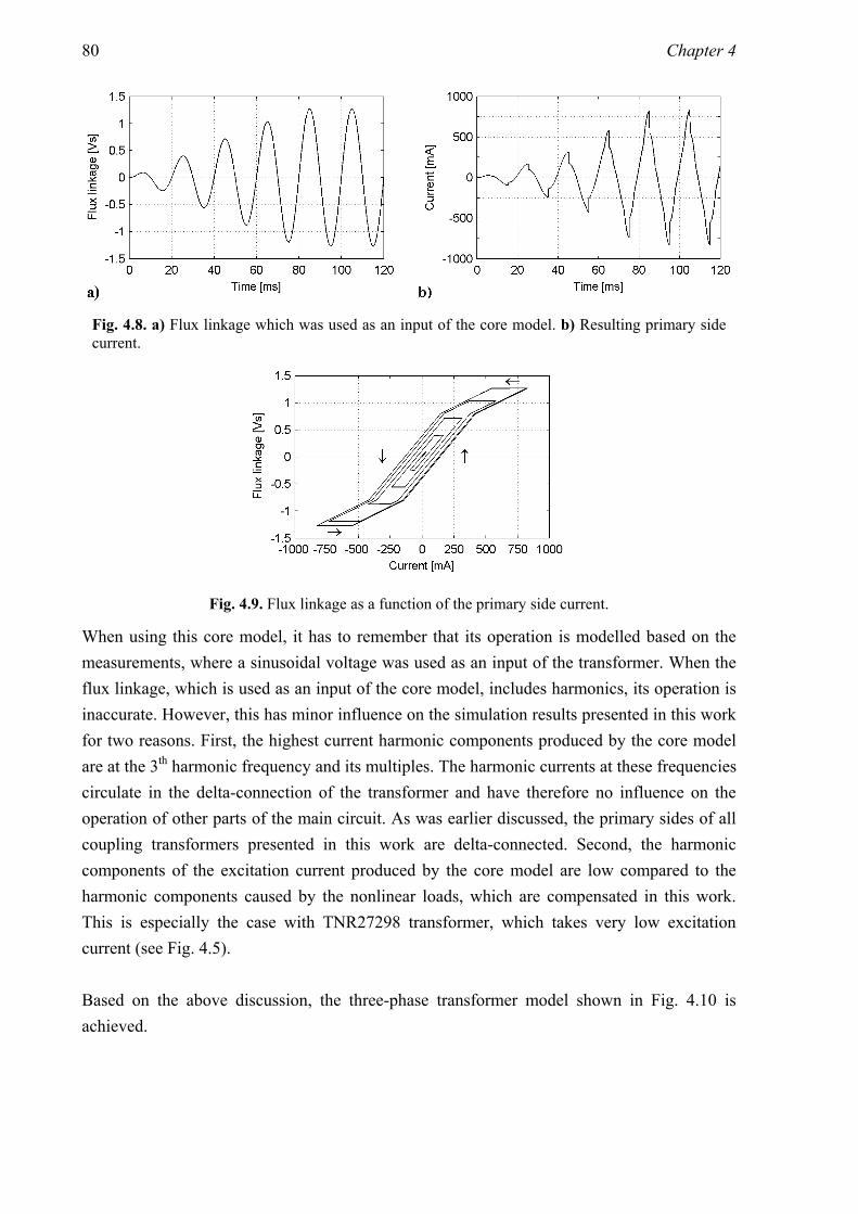
80 Chapter 4
Fig. 4.8. a) Flux linkage which was used as an input of the core model. b) Resulting primary side current.
Fig. 4.9. Flux linkage as a function of the primary side current.
When using this core model, it has to remember that its operation is modelled based on the measurements, where a sinusoidal voltage was used as an input of the transformer. When the flux linkage, which is used as an input of the core model, includes harmonics, its operation is inaccurate. However, this has minor influence on the simulation results presented in this work for two reasons. First, the highest current harmonic components produced by the core model are at the 3th harmonic frequency and its multiples. The harmonic currents at these frequencies circulate in the delta-connection of the transformer and have therefore no influence on the operation of other parts of the main circuit. As was earlier discussed, the primary sides of all coupling transformers presented in this work are delta-connected. Second, the harmonic components of the excitation current produced by the core model are low compared to the harmonic components caused by the nonlinear loads, which are compensated in this work. This is especially the case with TNR27298 transformer, which takes very low excitation current (see Fig. 4.5). Based on the above discussion, the three-phase transformer model shown in Fig. 4.10 is achieved.

Modelling 81
u1A
u2A
R1
iexA
L1'+L2 R2
u2idAu1idA
i1deA
iexB
u1B
i1deB R1
u1idB u2idB
R2
u2B
iexC
u1C
i1deC R1
u1idC u2idC
R2
u2C
i1idA
i1idB
i1idC
i2A
i2B
i2C
i1A
i1B
i1C
L1'+L2
L1'+L2
Fig. 4.10. Three-phase transformer model.
In Fig. 4.10, the dashed lines are used to denote the connections that are not included in the transformer construction, i.e. the primary side of the transformer is delta-connected. In this model, the primary quantities are not reduced to the secondary side, as was shown in Fig. 4.4. Instead of this, an ideal transformer model is used to take account of the transformer transformation ratio. The current sources iexA, iexB and iexC are due to the saturation and hysteresis models of the iron core. The currents are dependent on the flux linkages of the phases. The flux linkages of each phase are calculated based on voltages u1idA, u1idB and u1idC. Based on Fig. 4.10, the delta-connected primary side is modelled using the following equations: 1deC1A1deA iii += (4.10)
1deA1B1deB iii += (4.11)
1deB1C1deC iii += (4.12)
The phase-A of the transformer is modelled using the following equations: exA1deA1idA iii += (4.13)
1deA11idA1B1A iRuuu −=− (4.14)
t
ud
d A1idA
ψ= (4.15)
( )AexA f ψ=i (4.16)
2A1
21idA i
NNi = (4.17)
1idA1
22idA u
NN
u = (4.18)
( )t
iLLiRuu
dd 2A
2'12A22idA2A +++= (4.19)

82 Chapter 4
(4.16) presents the dependency of the excitation current on the flux linkage, as is earlier explained. The three-phase Simulink implementation of the transformer is achieved by using these equations and by generating (4.13) – (4.19) for phases B and C.
4.3 Modelling of the supply connected topology
The space vector model of the supply connected topology (SCT) presented in Fig. 3.8 is shown in Fig. 4.11. The model is achieved using the space-vector theory presented in Chapter 3 and in the previously presented component models.
C5
RsupdcLsup1
usup
Csf iCsf
Lsf3Rsf3
usfCdc
isup
i1
isf
Supply
APF
Load
ilo
ih ip
uloRsup1
Lsup2
Rsup2
Lsup3
Rsup3
Transformer model+SVT
Lsf2Rsf2
Rsf1 Lsf1
Rsfdc
L53R53
R5dc
R51 L51
R52 L52
i5
R7dc
R71 L71
R73
R72
C7
i7
L73
L72
Lhp1
Lhp2
Lhp3
Rhp1
Rhpdc
Rhp3
Rhp2
Chp
ihp
Rhp
u2
u1
Fig. 4.11. Space vector model of the SCT.
The supply voltage is presented as a voltage source usup. Since the impedance of the load is assumed to be infinity in the simulations, the load is presented as current sink ilo. The inverter of the APF is presented as a voltage source usf. The transformer is modelled as is described in Section 4.2.3. Since the transformer is modelled per phase basis and the rest of the model is implemented using space vector theory, the space vector transformation has to be done for the three-phase quantities received from the transformer model (i1ABC and isupABC) and inverse transformation for the space vector quantities fed to the transformer model (u1 and u2). This is denoted as “+SVT” in Fig. 4.11. In Fig. 4.11, the currents through the resistances and inductances of the RL blocks of the modelled inductors have not been named in order to get a clearer figure. However, in the

Modelling 83
following equations, these currents are denoted using the name of that component as a subscript of the current, e.g. the current flowing through the inductance L52 is denoted as iL52. The directions of the currents through the components of the RL blocks are the same as the current direction of the modelled inductor. In addition to this, in the following equations it has to be noticed that the secondary side current of the coupling transformer is equal to the supply current in the case of the SCT, i.e. i2 = isup. In the model of the SCT, isup is calculated in the block that models the transformer. Based on Fig. 4.11 and the above discussion, the following space vector presentation of the system is achieved. The space vector models of the inverter and its LC filter are achieved using the following equations.
∫= tiC
u d1Csf
sf1 (4.20)
sfsfdcRsf1sf1Rsf2sf2Rsf3sf3sf1 iRiRiRiRuu ++++= (4.21)
Csfsf1 iii += (4.22)
3,2,1,d
dRsfsf
sfLsf == niR
ti
L nnn
n (4.23)
3,2,1,LsfRsfsf =+= niii nn (4.24)
The unknown variables are solved based on these equations. The solved equations are used to model the inverter and its LC-filter. Excluding the coupling transformer, the rest of the main circuit is modelled using the following equations.
Supply branch
Rsup3sup3Rsup2sup2Rsup1sup1supsupdc2losup iRiRiRiRuuu ++++=− (4.25)
3,2,1,d
dRsupsup
upLssup == niR
t
iL nn
nn (4.26)
3,2,1,LsupRsupsup =+= niii nn (4.27)
Passive filter tuned for 5th harmonic frequency
55dcR5151R5252R535355
lo d1 iRiRiRiRtiC
u ++++= ∫ (4.28)
3,2,1,d
dR55
5L5 == niR
ti
L nnn
n (4.29)
3,2,1,L5R55 =+= niii nn (4.30)

84 Chapter 4
Passive filter tuned for 7th harmonic frequency
77dcR7171R7272R737377
lo d1 iRiRiRiRtiC
u ++++= ∫ (4.31)
3,2,1,d
dR77
7L7 == niR
ti
L nnn
n (4.32)
3,2,1,L7R77 =+= niii nn (4.33)
High-pass filter
phphphp
lo d1 iRtiC
u += ∫ (4.34)
3,2,1,d
dRhphp
hpLhp == niR
ti
L nnn
n (4.35)
3,2,1,LhpRhph =+= niii nn (4.36)
hhpdcRhp1hp1Rhp2hp2Rhp3hp3php iRiRiRiRiR +++= (4.37)
phhp iii += (4.38)
Main circuit currents
lohp75sup iiiii +++= (4.39)
These equations are used to model the main circuit in the simulations in addition to inverter equations (4.20) – (4.24) and the transformer model presented in Section 4.2.3. In the previous case the LC-filter was used in the output of the APF. If the system is modelled in the case where the LC-filter is not used, the model of the system is simpler. In this case (4.20) - (4.24) do not need to be taken into account and the primary side voltage and current of the coupling transformer are equal to the output voltage and current of the inverter, i.e. u1 = usf and isf = i1. The main level of the Simulink implementation of the space vector model of the SCT is presented in Fig. 4.12. The simulation model was made using the Simulink-expansion of the Matlab software. The implementation consists of two subsystems. These are the models of the APF and the rest of the main circuit. The subsystem “APF” includes the models of the control system, the space vector modulator and the inverter. The control system is modelled based on the control system shown in Fig. 3.10. The space vector modulator is modelled based on its operating principle as discussed in Section 3.1.1. The inverter is modelled using (3.24), (4.2) and (4.4). The subsystem “main circuit” includes the models of the coupling transformer and other passive components included in the main circuit. Besides the two subsystems, the model

Modelling 85
includes two sources, which are the supply voltage and the load current. The load current is modelled as a current source, since the load impedance is assumed to be infinity. The waveforms of the supply voltage and the load current are taken from the measurements of the SCT prototype. Some details of the Simulink implementation are shown in Appendix B.
Out1
supply voltage
ilo_ABC
usup_ABC
usf _ab
ulo_ABC
isup_ABC
isf _ab
main circuit
load voltage
Out1
load current
usup_ABC
isup_ABC
isf _ab
usf _ab
APF
Fig. 4.12. Simulink implementation of the SCT.
4.4. Modelling of the filter connected topology
The space vector model of the filter connected topology (FCT) presented in Fig. 3.11 is shown in Fig. 4.13. The model is achieved using the space vector theory presented in the Chapter 3 and the component models presented in the beginning of this chapter. Similarly to the SCT, the supply voltage usup and the load current ilo are presented as sources. The transformer is modelled as described in Section 4.2.3. In the FCT the secondary side current of the coupling transformer is equal to the total current of the LC shunt circuits, i.e. i2 = if. In the FCT model if is calculated in the transformer model. The inverter and its LC filter are modelled similarly as with the SCT using (4.20) – (4.24). If the system is modelled without the LC-filter, (4.20) - (4.24) do not need to be taken into account and the primary side voltage and current of the coupling transformer are equal to the output voltage and current of the inverter, i.e. u1 = usf and isf = i1.

86 Chapter 4
C5
RsupdcLsup1
usup
usfCdc
isup
Supply
APF
Load
ilo
ih ip
uloRsup1
Lsup2
Rsup2
Lsup3
Rsup3
Transformer model+SVT
L53R53
R5dc
R51 L51
R52 L52
i5
R7dc
R71 L71
R73
R72
C7
i7
L73
L72
Lhp1
Lhp2
Lhp3
Rhp1
Rhpdc
Rhp3
Rhp2
Chp
ihp
Rhp
u2u1
Lsf1 Lsf2 Lsf3
Rsf1 Rsf2 Rsf3isf
Csf
iCsf
Rsfdc i1 if
Fig. 4.13. Space vector model of the FCT.
Based on Fig. 4.13, the main circuit of the FCT can be modelled as follows. Because of the similarities between the SCT and the FCT, (4.26), (4.27), (4.29), (4.30), (4.32), (4.33) and (4.35) – (4.39) are used also in the FCT modelling. In addition to this, the following equations are used. Rsup3sup3Rsup2sup2Rsup1sup1supsupdclosup iRiRiRiRuu +++=− (4.40)
55dcR5151R5252R535355
2lo d1 iRiRiRiRtiC
uu ++++=− ∫ (4.41)
77dcR7171R7272R737377
2lo d1 iRiRiRiRtiC
uu ++++=− ∫ (4.42)
phphphp
2lo d1 iRtiC
uu +=− ∫ (4.43)
hp75f iiii ++= (4.44)
The main level of the Simulink implementation of the FCT is similar to the one of the SCT presented in Fig. 4.12. The implementation similarly includes two subsystems. The first one includes the models of the control system, the space vector modulator and the inverter. The control system is modelled based on the control system presented in Fig. 3.13. The space
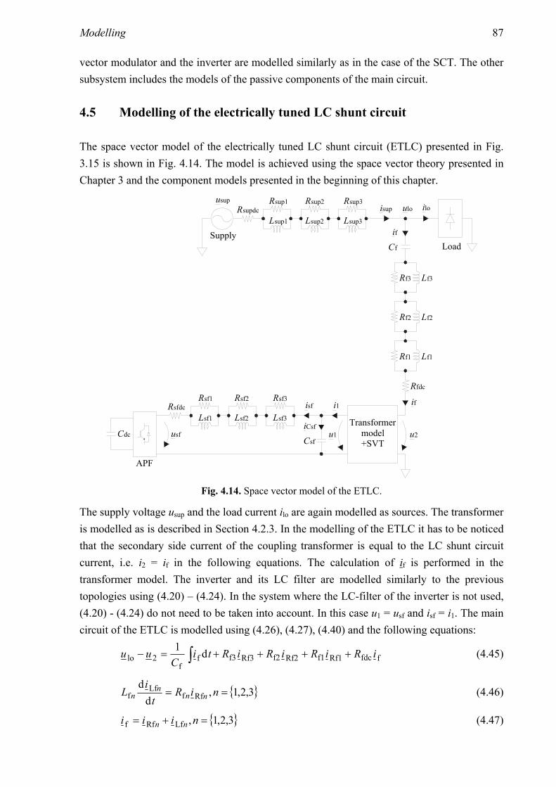
Modelling 87
vector modulator and the inverter are modelled similarly as in the case of the SCT. The other subsystem includes the models of the passive components of the main circuit.
4.5 Modelling of the electrically tuned LC shunt circuit
The space vector model of the electrically tuned LC shunt circuit (ETLC) presented in Fig. 3.15 is shown in Fig. 4.14. The model is achieved using the space vector theory presented in Chapter 3 and the component models presented in the beginning of this chapter.
Cf
RsupdcLsup1
usup
usfCdc
isup
Supply
APF
Load
ilouloRsup1
Lsup2
Rsup2
Lsup3
Rsup3
Transformer model+SVT
Lf3Rf3
Rfdc
Rf1 Lf1
Rf2 Lf2
if
u2u1
Lsf1 Lsf2 Lsf3
Rsf1 Rsf2 Rsf3isf
Csf
iCsf
Rsfdc i1 if
Fig. 4.14. Space vector model of the ETLC.
The supply voltage usup and the load current ilo are again modelled as sources. The transformer is modelled as is described in Section 4.2.3. In the modelling of the ETLC it has to be noticed that the secondary side current of the coupling transformer is equal to the LC shunt circuit current, i.e. i2 = if in the following equations. The calculation of if is performed in the transformer model. The inverter and its LC filter are modelled similarly to the previous topologies using (4.20) – (4.24). In the system where the LC-filter of the inverter is not used, (4.20) - (4.24) do not need to be taken into account. In this case u1 = usf and isf = i1. The main circuit of the ETLC is modelled using (4.26), (4.27), (4.40) and the following equations:
ffdcRf1f1Rf2f2Rf3f3ff
2lo d1 iRiRiRiRtiC
uu ++++=− ∫ (4.45)
3,2,1,d
dRff
Lff == niR
ti
L nnn
n (4.46)
3,2,1,LfRff =+= niii nn (4.47)

88 Chapter 4
lofsup iii += (4.48)
The main level of the Simulink implementation of the space vector model of the ETLC is presented in Fig. 4.15. The implementation includes two subsystems as was the case with previous topologies. The one includes the models of the control system, space vector modulator and inverter, and the other the model of the main circuit. The control system is modelled based on the control system presented in Fig. 3.17. The space vector modulator and the inverter are modelled similarly as with previous topologies.
Fig. 4.15. Simulink implementation of the ETLC.
4.6 Modelling of the UPQC
The space vector model of the unified power quality conditioner (UPQC) presented in Fig. 3.19 is shown in Fig. 4.16. The model is achieved using the space-vector theory presented in Chapter 3 and the component models presented in the beginning of this chapter. In Fig. 4.16, the supply voltage is presented as a voltage source usup, load current as a current sink ilo and the output voltages of the SAPF and the PAPF as voltage sources usf and upf. The coupling transformer shown in Fig. 4.16 is modelled based on the principles discussed in Section 4.2.3. However, no supply inductor is used in the case of the UPQC. The supply impedance is modelled as a series connection of the supply resistance and the supply inductance. In the modelling, the supply resistance and impedance are included in the transformer equations. Therefore, (4.19) used in transformer modelling is replaced by the following equation in the case of the UPQC:
( )t
iLLiRt
iLiRuuud
dd
d 2A2
'12A2
2Asup2Asup2idAloAsupA +++++=− (4.49)
In the above equation it has to be noticed that in the UPQC the secondary side current of the coupling transformer of the SAPF is equal to the supply current, i.e. i2=isup.

Modelling 89
Rsupusup
SupplyLoad
iloulo
Lpm3Rpm3
Rpmdc
Rpm1 Lpm1
Rpm2 Lpm2
Lsup
APF
usf
Rsfdc
Rsf1 Lsf1
Rsf3 Lsf3
Csf
isf
iCsf
Transformer model+SVT
u2
i1u1
isup
Cdc
APF
upf
Rpm
iRpm ipmi
ipm
Lpf2
Lpf1
Rpfdc
Rpf1
Rpf2
Lpf3Rpf3
ipf
Cpf
iCpf
Rsf2 Lsf2
idc,SAPF idc,PAPF
Fig. 4.16. Space vector model of the UPQC.
The rest of the main circuit of the UPQC is modelled as is next described. The SAPF is modelled similarly to the SHAPF topologies using (4.20) – (4.24). The rest of the main circuit is modelled using the following space vector presentation, which is based on Fig. 4.16.
LCL-filter (main circuit side)
pmiRpmpm iii += (4.50)
3,2,1,d
dRpmpm
pmLpm == niR
t
iL nn
nn (4.51)
3,2,1,LpmRpmpmi =+= niii nn (4.52)

90 Chapter 4
Rpm3pm3Rpm2pm2Rpm1pm1pmipmdcRpmpm iRiRiRiRiR +++= (4.53)
∫+= tiC
iRu d1Cpf
pfRpmpmlo (4.54)
LCL-filter (inverter side)
pmiRpmCpfpf iiii +=+ (4.55)
3,2,1,d
dRpfpf
pfLpf == niR
t
iL nn
nn (4.56)
3,2,1,LpfRpfpf =+= niii nn (4.57)
Rpf3pf3Rpf2pf2Rpf1pf1pfpfdcpfCpfpf
d1 iRiRiRiRutiC
++++=∫ (4.58)
Main circuit currents
lopmsup iii += (4.59)
The system is modelled by solving the unknown variables from the above equations. However, it has to be noticed that the voltage vector u2, which appears in Fig. 4.16, is left unsolved. The main level of the Simulink implementation of the space vector model of the UPQC is presented in Fig. 4.17.
Out1
supply voltage(fund. comp.)
Out1
supply voltage
supply current
ilo_ABC
usup_ABC
usf _ab
upf _ab
isup_ABC
ulo_ABC
isf _ab
ipf _ab
main circuit
Out1
load current
usup_ABC
ulo_ABC
isf _ab
Udc
usup_f und
usf _ab
Idc_SAPF
SAPF
Idc_SAPF
usup_f und
ilo_ABC
ulo_ABC
ipf _ab
upf _ab
Udc
PAPF
[usup_fund]
[Udc]
[i lo_ABC]
[usup_ABC]
[usup_fund]
[Udc]
[i lo_ABC]
[usup_fund]
Fig. 4.17. Simulink implementation of the UPQC.
The implementation includes three subsystems, which are called “SAPF”, “PAPF” and “main circuit”. Subsystem “SAPF” includes the control system, space vector modulator and inverter

Modelling 91
of the SAPF. Respectively, the subsystem “PAPF” includes the control system, space vector modulator and inverter of the PAPF. The control system of the SAPF is modelled on the control system shown in Fig. 3.21 and the control system of the PAPF is modelled on the control system shown in Fig. 3.22. The space vector modulators of both APFs are modelled on the operating principles discussed in Section 3.1.1. The inverters of both APFs are modelled based on (3.24) and (4.2). In addition to this, an equation which is used to calculate the dc-link voltage is needed. In the case of the UPQC the inverters have a common dc-link. Therefore, in the modelling of the dc-link (4.4) is replaced with the equation which combines the models of two inverter bridges. This equation is achieved using the Kirchhoff’s current law. Based on the law and Fig. 4.16,
dc
dcdcdcSAPF,dcPAPF,dc d
dRu
tu
Cii +=+ , (4.60)
where idc,PAPF is the dc-current of the PAPF inverter bridge and idc,SAPF is the dc-current of the SAPF inverter bridge. Based on the previous equation, the dc-link voltage udc may be calculated. This equation is used in modelling to combine the models of the PAPF and the SAPF inverter bridges.
tRu
iiC
u d1
dc
dcSAPFdc,PAPFdc,
dcdc ∫ ⎟⎟
⎠
⎞⎜⎜⎝
⎛−+= , (4.61)
The subsystem “main circuit” includes the models of the passive components of the main circuit. In addition to the three subsystems, the implementation includes three sources, which are the load current, the supply voltage and the fundamental component of the supply voltage, whose amplitude is constant. The fundamental component of the supply voltage, whose amplitude is constant, is needed in the simulations of the UPQC in order to generate the angle of the supply voltage oriented synchronous reference frame. This is because in the simulations the angle is calculated straight based on the space vector of the supply voltage. Since in the simulations and the tests distorted supply voltage is also used, this would create errors to the angle of the synchronous reference frame. In the prototype this does not happen since the angle is generated using a phase locked loop (PLL).
4.7 Simulation model imperfections
The simulation and prototype test results presented in this work are achieved using equal parameters in order to have comparable results. Despite this, there are differences between the simulation and test results. The errors are due to imperfections of the simulation models, which are next discussed.

92 Chapter 4
The first known imperfection is incomplete modelling of the passive components. This is because in reality the parameters of the passive components change as a function of several quantities and therefore their complete modelling is difficult. The current harmonics filtering of the presented SHAPFs is based on the division of the harmonic components of the load current between the supply branch and the filter branches. Therefore, if the behaviour of the passive components of the main circuit is incompletely modelled, also this current division is incorrect, which leads to an error in the simulated supply current THD. The second imperfection is the load current used in the simulations. In the simulations, the load current waveform, which was achieved in the prototype measurements, is used as an input of the simulation models. This was done in order to make the processing time of the simulation models reasonable. Since this was done, it had to be assumed that the load current is independent on the load voltage. This assumption is valid at the harmonic frequencies in the case of the used rectifier load, where the load impedance is high. Since the load impedance is high, small variations occurring in the load voltage have insignificantly small influence on the load current. However, since the load impedance is not infinity, the error is caused between the simulation and measurement results. The dependency of the load current and the load voltage on the used harmonic filter is inspected closely in Appendix D. The inspection is made in the cases of the RL and RC-type nonlinear loads used in this work. Both of these loads consist of a three-phase diode rectifier. In the case of the RL-type nonlinear load the inductor and the resistor are connected in series on the dc-side of the diode rectifier. In the case of the RC-type nonlinear load the dc-side load consists of the parallel connected resistor and capacitor. As can be seen in the appendix, the load current THD is quite independent on the used filter if the RL-type nonlinear load is used. However, in the case where the RC-type nonlinear load is used, it can be seen that the load current THD varies with the used harmonic filter. The variation is biggest in the case of the FCT. Therefore, the simulation and the measurement results differ most in the case of the FCT when the RC-type nonlinear load is used. The third imperfection that has an influence on the simulation results is the incomplete modelling of the PWM-VSI. As was shown in the beginning of the chapter, the PWM-VSI is modelled ideally. Since PWM-VSI is not ideal in reality, errors are caused to the output voltage because of, e.g. the dead times between the component switchings.

Prototype realisation 93
5 Prototype realisation
The functioning of the inspected series hybrid active power filters (SHAPFs), i.e. the supply connected topology (SCT), the filter connected topology (FCT) and the electrically tuned LC shunt circuit (ETLC) in addition to the unified power quality conditioner (UPQC), was researched also using laboratory prototypes. The prototypes of each SHAPF and the UPQC were constructed and their performance measured. All topologies were implemented using the same pulse width modulated voltage source inverter (PWM-VSI) prototype. This PWM-VSI was used with other circuit elements needed to constitute each topology. The prototype realisation is discussed in this chapter. Detailed information of the prototype is presented in Appendix C.
5.1 Inverter prototype
The realisation of the PWM-VSI can be divided into realisation of the hardware and software. Both of these are presented next.
5.1.1 Hardware
The circuit diagram of the implemented three-phase PWM-VSI is presented in Fig. 5.1. The PWM-VSI prototype consists of three three-phase converters, of which two are controllable and one a diode rectifier. The two controllable inverters consist of six IGBTs and the diode rectifier respectively of six diodes. Besides the converters the PWM-VSI includes the dc-link capacitor Cdc, discharge resistor Rdc, safety resistor Rov, three-phase contactors SWc1, SWc2 and SWc3 and the control circuits of the IGBT bridges. In addition to the components shown in Fig. 5.1, several other components, such as measurement and relay boards, are included in the prototype. The two inverters are used as voltage sources of the series active power filter (SAPF) and the parallel active power filter (PAPF). The inverter of the SAPF is on the left hand side and the inverter of the PAPF on the right hand side in Fig. 5.1. The diode rectifier is not normally used, but it is used in some special tests. These tests are executed with the SCT and FCT. In these cases only the SAPF, whose dc-link voltage controller is disabled, is used, and the diode rectifier is used as an auxiliary power supply to maintain the dc-link voltage. The switching signals of the IGBT bridges of the SAPF and the PAPF are calculated by two microcontrollers and amplified by the driver circuits.

94 Chapter 5
Cdc Rdc
Rov
PLA
TPU
MPC-563SCI
ADA
IC0ADB
IO0
drivers
PC
TPU
SCI
PLA
drivers
meas.
IC1IC2
IO1signals
SW c1
SW c2
SW c3
SW c1SW c2
oc sig.
ov sig.usupA
ov sig.
meas.signalsoc sig.uloA
IC2
ADBADA
IC1IC0
IO0 SW c3
MPC-563SCI
Fig. 5.1. Implemented PWM-VSI.
Microcontroller board
The microcontroller boards used with the SAPF and the PAPF are identical. Both of the microcontroller boards include the microcontroller, the memory circuits, a part of the measurement circuits and the logic circuits used to generate the switching reference signals. The model of the microcontroller is MPC-563 and it is manufactured by Motorola. Its most important features are given in Appendix C. The operation and the features of the microcontroller board, such as the current and voltage measurement circuits, are presented in (Levonen, 2006). The microcontroller generates the output voltage reference vector, which is then used to calculate the switching times of the IGBTs. In order to calculate the output voltage reference vector, the microcontroller gathers the necessary measurement data from the main circuit. In addition to this, the microcontroller also takes care of the safe operation of the active power filter (APF). The microcontroller also provides a connection for the PC, which is used to monitor the operation of the APF and to change the control parameters. When the APF is operating, the currents and voltages are first measured by the measurement boards for the control system. The processed measurement signals are fed to the A/D-converters of the microcontroller. In MPC-563, there are two A/D-converter modules, which

Prototype realisation 95
are denoted as ADA and ADB in Fig. 5.1. The output voltage reference vector is calculated by the control system after this. Next, the switching times of the IGBTs are calculated by the space vector modulator. The switching times are then stored in the memory. Based on the stored switching times, the logical states of the microcontroller output channels are managed by the time processor unit of the microcontroller (TPU). The output signals of the microcontroller are transferred to the programmable logic array (PLA) circuit, which generates the final switching signals. The final switching signals are amplified by the driver circuits and used to switch the IGBTs. The operation of the space vector modulator is based on the operating principles discussed in Section 3.1.1. Its microcontroller implementation, which was discussed shortly above, is presented more closely in (Routimo, 2002). However, the implementation of the PLA logic differs from the one presented in the reference. Instead, the PLA logic shown in (Pettersson, 2004) is used in this work. Input capture channels IC0…2 are used to protect the inverter and to synchronise it with the supply voltage. The microcontroller board includes a comparator circuit, which monitors all measured current signals. It compares the amplitudes of the currents with the predefined value and whenever it detects an overcurrent, an output signal is produced. IC0 channel monitors the output signal of the comparator, which is denoted as “oc sig.” in Fig. 5.1. When the overcurrent is detected by the input capture channel IC0, the inverter is shut down immediately. This same procedure applies also to the dc-link voltage. When the overvoltage is detected, the comparator produces an output signal which is detected by the input capture channel IC2. The output signal of the comparator is denoted as “ov sig.” in Fig. 5.1. The input capture channel IC1 is used to synchronise the inverter. In the case of the SAPF the phase-A supply voltage usupA is monitored by the comparator. Whenever zero voltage crossing is detected, an output signal is produced. This is detected by the microcontroller input capture channel IC1. This signal is used to synchronise the phase-locked loop (PLL), which is used to set the angle of the space vector reference frame. In the case of the PAPF the procedure is similar, but the output voltage is synchronised with the phase-A load voltage uloA. The general purpose I/O-pins IO0 and IO1 are used as digital outputs to produce the switching signals to contactors SWc1, SWc2 and SWc3. IO0 and IO1 are not used to switch the contactors directly but are used to control the relays on the relay board, which are then used to control the three-phase contactors. The purpose of the contactors is to protect the PWM-VSI against overcurrents and overvoltages. In the cases of both microcontrollers, IO0 is used in the charging of the dc-link voltage. If the dc-link voltage was low and the supply voltage was applied on the ac-side of the diode

96 Chapter 5
rectifier or of the inverter of the PAPF, high inrush current would occur. This inrush current is limited using the resistors, which are bypassed using the contactors SWc1 and SWc3 when the dc-link voltage is on the safe level. On the ac-side of the inverter of the SAPF the contactor is not used. This is because the inverter of the SAPF is connected to the main circuit using the coupling transformer and therefore no inrush current can occur. In addition to this, in the case of the SCT the SAPF is connected in series with the supply and therefore switching off the contactor would shut off the load current, which is not a desirable situation. IO1 signal of the SAPF microcontroller is used to protect the IGBTs against overvoltages. In normal operation, there is no current through the resistor Rov since the contactor SWc2 is not conducting. However, if overvoltage in the dc-link is observed, the contactor is switched to the conducting state to lower the dc-link voltage to the safe level. The serial connection interface (SCI) is used to connect the microcontroller to the PC using RS-232 bus. The PC is used to monitor the operation of the APF and to change the control system parameters.
Measurement boards
The PWM-VSI prototype includes several current and voltage measurement boards. All currents are measured using similar current measurement boards. The current measurement circuits are based on LEM LA 55-P current transducers. The transformation ratio of the transducers is tuned such that the maximum amplitude of the ac-current that can be measured is 25 A and the resolution of the measurement is 49 mA. The current measurement board that is used to measure the supply current also includes the measurement circuit for the synchronisation signal. Three different voltage measurement boards are used to measure the dc-link voltage, supply voltage and load voltage. The dc-link voltage measurement is based on the differential amplifier made of operational amplifiers. The maximum dc-link voltage which can be measured is 1005 V and the resolution of the measurement is 0.98 V. The supply voltage measurement is based on the operational amplifier circuit. The maximum amplitude of the ac-voltage which can be measured is 445 V and the resolution of the measurement is 0.87 V. The load voltage measurement is based on a simple resistor circuit. The maximum amplitude of the measured ac-voltage and the resolution of the measurement are the same as with the supply voltage measurement board.
Relay board
The prototype of the PWM-VSI includes three three-phase contactors, as was earlier mentioned. The switching of the contactors requires 230 V input signal and therefore they can

Prototype realisation 97
not be switched using the output signals of the microcontroller. In order to amplify the output signals of the microcontroller, the relay board was designed. The operation of the board is based on the switching of OMRON G6RN relay using the signal, which is first received from the microcontroller and then amplified using BC546 transistor. The operation of the relay board is described in detail in (Turunen, 2003).
Power supply and driver board
The microcontroller boards, measurement boards, relay boards and driver circuits need power supplies at different voltage levels. For this purpose, the prototype of the PWM-VSI includes a board where the necessary voltages are generated. The input voltage for this board is 24 Vac, which is produced from the 230 V supply voltage by a step-down transformer. The output voltage levels of the board are 8 Vdc (regulated and unregulated), +/-12 Vdc, +/-15 Vdc and 24 Vdc. This same board also includes the driver circuits of the IGBTs. The inputs of the driver circuits are +5/0 Vdc switching reference signals produced by the microcontroller board. The driver circuit amplifies the input voltages to +/-15 Vdc voltage signals, which are used to drive the IGBTs.
5.1.2 Software
When the APF is operating, the microcontroller measures the needed quantities using A/D-converters and performs the calculation of the output voltage reference vector based on the measurement results. After this it generates switching signals of the IGBTs according to the output voltage reference vector. In addition to this, the microcontroller monitors the operation of the APF for possible overvoltages and overcurrents and takes care of communication with the PC. All this is done according to the commands implemented in the software. The commands are executed in pace with the interruptions that are made by the microcontroller timer unit. The interruption interval of the microcontroller is 50 μs with all APFs in this work. In the space vector modulator 10 kHz modulation frequency is used, i.e. the switching times of the IGBTs are calculated twice in a modulation period. The softwares of the APFs were written using C/C++ programming language and RCPU instructions. The most essential part of the software is the interrupt servicing routine, which defines the sequence where the operations of the APF are executed. Although the control systems of the APFs are different, their interrupt servicing routines are similar. According to the interrupt servicing routine, the tasks of APF are performed using the following sequence.
1. Fault detection. The overvoltage and overcurrent flags are detected. If there is a fault the APF is shut down.
2. Measurements. The measurement results are read from the A/D-converters. 3. Control. The output voltage reference vector is calculated based on the measurement

98 Chapter 5
results. 4. Modulator updating. The calculated output voltage reference vector is fed to the
space vector modulator, which calculates and stores to memory the switching times of the IGBTs.
5. SCI processing. The data is transferred to the PC and received from the PC using the RS-232 bus.
6. Synchronisation. If zero crossing of the reference voltage is detected, the PLL is synchronised. In the case of the SAPF, the software is synchronised with the supply voltage and in the case of UPQC, the software of the PAPF is synchronised with the load voltage.
The order of the execution of the tasks also defines their priority order. The most important tasks are performed first and less important ones last. With this it is assured that there is enough time to execute at least the most important tasks at every cycle. In addition to this, not all of these tasks are executed at every cycle in order to prevent unnecessary calculations. The third item in the previous list is the execution of the control system. All other control events are executed at every cycle, but the dc-link control is executed only at every 20th cycle, i.e. at an interval of 1 ms. The detection of the synchronisation signal, which is the last item on the list, is executed at every 40th cycle, i.e. at an interval of 2 ms.
5.2 Structures of SHAPFs and UPQC
The prototypes of the SHAPFs and the UPQC were created based on their main circuits, shown in Chapter 3. Basically, the main circuits of the SCT, FCT and ETLC are made of similar circuit elements: the power supply, SAPF, passive filters and the load. In the case of UPQC there is the power supply, SAPF, PAPF and the load. The design of these main circuit elements is presented in this subchapter. The parameters of the main circuits are presented in Appendix C. As can be seen in the main circuits shown in the Chapter 3, the main circuit of the SAPF is similar in each SHAPF topology. The main circuit of the SAPF consist of the PWM-VSI, LC-filter and coupling transformer.
LC-filters
The LC-filters were designed to filter the high frequency ripple of the inverter output voltage. The same LC-filter was used with the SCT and FCT. Since the LC-filter is a low-pass filter, the resonance frequency of the LC-filter was designed to be as low as possible in order to achieve a good filtering result. The lowest possible resonance frequency is limited by the filtering band of the SAPF, which was about 2 kHz in practice in the case of all topologies. The resonance frequency 3.8 kHz was used with the SCT and the FCT.

Prototype realisation 99
With the ETLC, however, lower resonance frequency was used. This was because of the problems in its dc-link voltage control. By using the same LC-filter as with SCT and FCT, the dc-link voltage could not be increased as high as was desired. This is because the APF is connected in series with only one LC shunt circuit in the case of the ETLC and therefore the current flowing through the SAPF at the fundamental frequency is lower than with the SCT or FCT. Because of this, the SAPF is capable of taking less real power at the fundamental frequency compared to cases of the SCT and FCT. Because of this, the higher inductance of the LC-filter inductor has to be used to minimise the real power inductor losses and to make it possible to maintain the desired dc-link voltage. Because of the higher inductance of the LC-filter inductor, the resonance frequency of the LC-filter is lower. The resonance frequency 2.3 kHz was used with the ETLC. In the case of the UPQC the amplitude of the switching frequency harmonics of the SAPF compensation voltage was desired to be low, and therefore a slightly higher capacitance was used in its LC-filter compared to the SHAPFs in order to decrease its resonance frequency. The resonance frequency 2.2 kHz was used with the UPQC.
Coupling transformers
The coupling transformers, which were used to inject the compensation voltage produced by the inverter, consisted of three single-phase transformers. The current ratings of the coupling transformers were designed somewhat higher than those required by the applications to minimise the copper losses. In addition to this, the transformer cores were designed to have smaller iron losses compared to ordinary power transformers. Because of the different performance requirements of the applications, two transformers were used. In the case of the SCT, FCT and ETLC, the purpose was only to filter the harmonics of the supply current. On the other hand, in the case of UPQC the purpose was to compensate the harmonics and the voltage dips of the supply voltage. Because of the different compensation requirements, higher compensation voltage is required in the case of UPQC, and therefore a different coupling transformer was used with the UPQC. The transformation ratio of the coupling transformer was 2:1 in the case of UPQC and 10:1 in the case of other topologies (the primary side is on the inverter side; see, e.g. Fig. 4.11).
Passive filters
Passive filters were included in the SCT, FCT and ETLC. In the cases of the SCT and FCT the same passive filters were used. Two of these filters were LC shunt circuits tuned for 5th and 7th harmonic frequency component and the third was a high-pass filter tuned for 11th harmonic. The actual resonance frequencies of these filters were designed to be slightly below the harmonic frequencies to prevent resonance with the supply inductance. The reactive power produced by each passive filter was designed to be 20…25 % of the load power. Since
100 Chapter 5
the power of the load was 3.8 kVA, the total reactive power produced by the three passive filters was about 2.5 kVAr. Since the reactive power taken by the load was only 600 Var (nonlinear RL-type load) or 900 Var (nonlinear RC-type load) this leaded to the situation, which is generally not desirable, i.e. more reactive power was produced by the passive filters than was taken by the load. However, this decision had to be done in the design of the passive filters since otherwise the inductance of the passive filter coils would have been unreasonable high to be implemented. The LC shunt circuit of the electrically tuned LC shunt circuit (ETLC) was tuned for 261 Hz. The LC shunt circuit of the ETLC was purposely mistuned, and as will be seen in Chapter 6, this mistuning led to a situation where the LC shunt circuit resonated with the supply. However, with the ETLC it is the task of the SAPF to tune the resonance frequency of the LC shunt circuit electrically. Since the resonance frequency of the LC shunt circuit is changed, also the resonance is removed when the SAPF is turned on. The reactive power produced by the LC shunt circuit was designed to be 25 % of the power of the load in the case of the ETLC.
LCL-filter of the PAPF
The main circuit of the PAPF of the UPQC consists of the PWM-VSI and LCL-filter. The LCL-filter was used since the harmonic content of the load voltage at the switching frequency was desired to be as small as possible. The resonance frequency of the LCL-filter used was 2.3 kHz. 100 Ω damping resistors were used with the LCL-filter, as presented in Fig. 3.19, in order to prevent oscillations.
Power supply
In addition to the presented main circuit components, also three-phase power supply and the load were included. In the case of the SCT, FCT and ETLC a 230/400 V power supply with a nominal frequency of 50 Hz was used. With the UPQC, ELGAR SW 5250A linear three-phase power supply was used. This power supply was used to generate distortions to the supply voltage, which were then compensated using the SAPF. In the case of the SCT, FCT and ETLC, also a supply inductor was used. In reality, the power rating of the SHAPF applications is significantly higher than those of the laboratory prototypes. The supply inductor was used to scale the supply impedance to the level corresponding to the used power rating. The inductance of the supply inductor was 3.7 %. This value was chosen, since the typical impedance of the 500 kVA distribution transformer is around 4 % (ABB, 2004). In the case of the UPQC the supply inductor was not used.
Prototype realisation 101
Loads
The loads were three-phase nonlinear RL and RC-type loads. The nonlinear RL-type load consisted of the series-connected inductor and resistor connected on the dc-side of the three-phase diode rectifier. Respectively, the non-linear RC-type load consisted of the parallel-connected capacitor and resistor connected on the dc-side of the three-phase diode rectifier. The power rating of the load was 3.8 kVA in the case of the SCT, FCT and ETLC and 2.4 kVA in the case of the UPQC. With the UPQC, a smaller power rating was used because of the current limitation of the power supply device.
102 Chapter 6
6 Operation of the SHAPFs and the UPQC
The operation of the three presented series hybrid active power filters (SHAPFs) and the unified power quality conditioner (UPQC) is dealt within this chapter. The operation is inspected through the results of the simulations and the experimental tests. The simulation results are obtained using the simulation models presented in Chapter 4 and the tests results using the prototypes presented in Chapter 5. The simulations and the tests are performed using the same parameters in order to achieve comparable results. The measurement results were achieved using an 8 bit digital oscilloscope. The resolution of all supply and load voltage measurements is 3.13 V. In the SHAPF measurements the resolution of the supply and load current measurements is 0.16 A and in the UPQC measurements 0.03 A. The beginning of the chapter presents the operation of the SHAPFs in steady-state operation and during dynamic changes. Based on the presented results, the current filtering performance of the SHAPFs is compared. After this the chapter presents the operation of the UPQC respectively. Last, a summary, which summarises the achieved results, is given.
6.1 Operation of the SHAPFs
The operation of the SHAPFs, i.e. the supply connected topology (SCT), filter connected topology (FCT) and electrically tuned LC shunt circuit (ETLC), is first researched. In stationary operation the simulations and tests are performed using three-phase, 3.8 kVA RL and RC-type nonlinear loads. Both of the loads consist of a three-phase diode rectifier. In the first case, an inductor and resistor are connected in series on the dc-side of the diode rectifier. In the second case the dc-side load consists of the parallel connected resistor and a capacitor. In the simulations and tests, where the behaviour of the dynamic load is inspected, only RL-type nonlinear load is used. The 230/400 V (50 Hz) supply voltage is used in all simulations and measurements. In stationary operation, the current filtering performance of the SHAPFs is inspected using various configurations. First, only the passive filters included in the SHAPFs are used in the current harmonics filtering. Next, the active power filter (APF) is connected. The simulations and the prototype tests are carried out in cases where there is LC-filter, and is not in the pulse width modulated voltage source inverter (PWM-VSI) output. The current harmonics filtering performance of the SCT and the FCT is also inspected in the case where the dc-link voltage control is disabled. In this case the dc-link voltage is maintained using a three-phase diode

Operation of the SHAPFs and the UPQC 103
rectifier. The current harmonics filtering performance of the ETLC is researched in the case of two control systems presented in Section 3.6. In the one control system the control of the active resistance Ract is not included in the control system and in the other it is. The best current filtering performance of the SHAPFs was found in the following ways. With the SCT and the FCT, the active resistance Ract was chosen to be as high as possible. This maximum value was limited by the characteristics of the prototype. The active resistance Ract was increased until the modulation index reached the value 0.66. If this value was largely exceeded, the resonance occurred in the SCT between the high-pass filter and the series active power filter (SAPF) at the frequency of about 2 kHz. The reason for this resonance is dealt with later. However, by using the modulation index 0.66 with the coupling transformer, whose primary side is delta-connected, the same compensation voltage is achieved on the secondary side of the coupling transformer as with using the modulation index 1.15 with the coupling transformer, whose primary side is wye-connected.
With the ETLC, however, the best possible filtering performance is achieved in a situation where the active reactances Xact,n produced by the SAPF are equal and opposite to the reactances of the LC shunt circuit at the harmonic frequencies whose ordinal number is n. This goal was achieved by applying the active inductances Lact,5 = 5.2 mH and Lact,7 = -4.4 mH in series with the LC shunt circuit using the SAPF. In the simulations and tests, where the control system that applies both active resistance Ract and active inductances Lact,n was used with the ETLC, Ract was chosen similarly as with the SCT and the FCT. The behaviour of the SHAPFs during the dynamic load change was simulated and tested using the RL-type nonlinear load. The dynamically varying load was realised by changing the load current stepwise by changing the value of the load resistor. In this test, the LC-filter was used in the output of the PWM-VSI with all topologies and the dc-link voltage controller was used to maintain the dc-link voltage of the SAPF. Although all simulated and tested systems were three phase systems, the results of only phase-A are presented. This is because all phase quantities are equal in a symmetrical three-phase system.
6.1.1 RL-type nonlinear load
This subchapter presents the results of the steady-state simulations and measurements, where the RL-type non-linear load was used.

104 Chapter 6
Current harmonics filtering performance of the passive filters
In this case only the passive filters included in the SHAPFs were used to filter the current harmonics and therefore the SAPF was not connected to the main circuit. Since the main circuits of the SCT and the FCT are similar if the SAPF is disconnected, also their filtering performances are similar. The simulation results in this case are presented in Fig. 6.1 and the corresponding measurement results in Fig. 6.2. The current filtering performances of the passive filters are presented in Tables 6.1 and 6.2. It must be noticed that in these and in all later tables and bar graphs, which present simulation or measurement results, the frequency components of the supply current are not presented as absolute values but as ratios of the respective frequency components of the load current. For sake of clarity, the current harmonics filtering performances are also presented as bar graphs in Figs. 6.3 and 6.4. In these bar graphs it has to be noticed that y-axis presents the ratio of the amplitudes of the frequency components, but “^”-symbols are not shown in the labels because of the software used for image processing. This applies also to the bar graphs presented later in this chapter. In Fig. 6.4, the height of the bar presenting the ratio of the current amplitudes at the 5th harmonic frequency in the case of the ETLC exceeds the upper limit of the y-axis. This ratio (156.1 %) is therefore marked above the bar. The heights of the bars, which exceed the upper limit of the y-axis are marked in this fashion also in later graphs.
Fig. 6.1. Simulated waveforms: a) load current, b) supply current in the case of the SCT and the FCT and c) supply current in the case of the ETLC.
Fig. 6.2. Measured waveforms: a) load current, b) supply current in the case of the SCT and the FCT and c) supply current in the case of the ETLC.
Based on these results it is seen that the harmonic content of the supply current is decreased when the passive filters of the SCT/FCT are used. Tables 6.1 and 6.2 show that the supply current THD is about ten percentage units smaller in this case compared to the load current THD. However, despite the filtering the THD value of the supply current still remains high.

Operation of the SHAPFs and the UPQC 105
Based on the simulation and measurement results it seems that the supply current THD is increased when the passive filter of the ETLC is used. As can be seen in Tables 6.1 and 6.2 as well as in Figs 6.3 and 6.4, the increasing of the THD is due to the increasing of the 5th harmonic component. The resonance occurring at the fifth harmonic frequency is due to the mistuning of the LC shunt circuit of the ETLC. The LC shunt circuit was purposely mistuned, since with the ETLC it is the purpose of the SAPF to tune the resonance frequency of the LC shunt circuit electrically. The tuning frequency of the LC shunt circuit is 261 Hz. It was chosen to be between the 5th and 7th harmonic component and close to the 5th harmonic component in order to minimise the needed compensation voltage of the SAPF. However, since the resonance frequency is close to the 5th harmonic component, an additional inductance, i.e. the supply inductor, makes it resonate.
Table 6.1. Simulated current harmonics filtering performance of the passive filters.
Load SCT FCT ETLC
n ni A,loˆ [A] n
n
ii
A,lo
A,supˆˆ
[%]n
n
ii
A,lo
A,supˆˆ
[%]
1 7.70 116.3 100.15 1.76 66.7 132.9 7 0.72 34.4 60.1
11 0.54 88.1 77.3 13 0.32 86.4 79.7 17 0.22 70.9 80.3 19 0.15 63.6 80.9 23 0.09 51.8 82.1 25 0.06 41.0 82.4 29 0.05 34.7 80.9 31 0.04 30.8 81.5 35 0.04 33.3 81.0 37 0.04 19.2 81.4 41 0.03 26.2 80.8 43 0.03 26.5 81.5 47 0.02 28.3 80.7 49 0.02 28.8 81.6
THD20kHz [%] 26.3 14.9 31.7
Table 6.2. Measured current harmonics filtering performance of the passive filters.
Load SCT FCT ETLC
n ni A,loˆ [A] n
n
ii
A,lo
A,supˆˆ
[%] n
n
ii
A,lo
A,supˆˆ
[%]
1 7.80 120.1 99.85 1.74 69.7 156.1 7 0.78 47.5 66.9
11 0.57 84.6 77.3 13 0.37 68.6 69.1 17 0.25 54.2 70.5 19 0.19 48.4 61.8 23 0.11 49.3 66.9 25 0.08 51.0 53.5 29 0.05 31.6 106.0 31 0.04 46.9 93.2 35 0.04 41.2 85.6 37 0.04 45.4 89.5 41 0.03 37.5 82.3 43 0.02 99.5 81.0 47 0.03 34.9 68.6 49 0.02 50.8 81.0
THD20kHz [%] 26.4 14.9 36.3 η [%] 95.4 95.4
Fig. 6.3. Simulated current harmonics filtering performance of the passive filters: SCT/FCT (black) and ETLC (white).

106 Chapter 6
Fig. 6.4. Measured current harmonics filtering performance of the passive filters: SCT/FCT (black) and ETLC (white).
The maximum permissible odd harmonic current components excluding the triplen harmonics according to harmonic standard IEC 61000-3-2 were presented in Table 2.1. If these results are compared to the values provided by the standard, it can be seen that if no filter is used with the load, the harmonic current components of the supply current are too high. If the passive filters of the SCT/FCT are used, it can be seen that the situation is improved. In this case the harmonic content of the supply current is almost within the limits provided by the standard. In the case of the ETLC the specifications provided by the standard are not fulfilled because of the resonance at the 5th harmonic frequency. The last row in Table 6.2 shows the efficiencies of the passive filters, which were calculated based on the oscilloscope measurements of the phase-A load and supply current and voltage. It seems that the efficiencies of the passive filters of the SCT/FCT and the ETLC were the same, although there are a different amount of passive filters in these topologies. However, this result is distorted by the resonance of the ETLC. Because of the resonance, a large current at the 5th harmonic frequency flows through the passive filter by causing additional losses. If there were no resonance, the efficiency of the passive filter of the ETLC would be higher. Based on the achieved results it can be stated that the simulation results agree quite well with the measurement results. If Tables 6.1 and 6.2 are compared, it is seen that the load current components are similar in the simulations and the measurements. This is because the measured load current waveform was used as a load current waveform in the simulations. However, the supply current components of the simulation results seem to differ slightly from the current components of the measurement results. This is because of the imperfections of the simulation models, which were discussed in Chapter 4.7.
Current harmonics filtering performance of the SHAPFs
The simulation and measurement results of the SCT, FCT and ETLC are presented next in the case where the APF is connected to the main circuit. In the first case the LC-filter is not used in the PWM-VSI output, but its output voltage is fed directly to the coupling transformer. The results are presented in Figs. 6.5 and 6.6 and in Tables 6.3 and 6.4. The current harmonics filtering performance of the SHAPFs is also presented as bar graphs in Figs. 6.9 and 6.11.
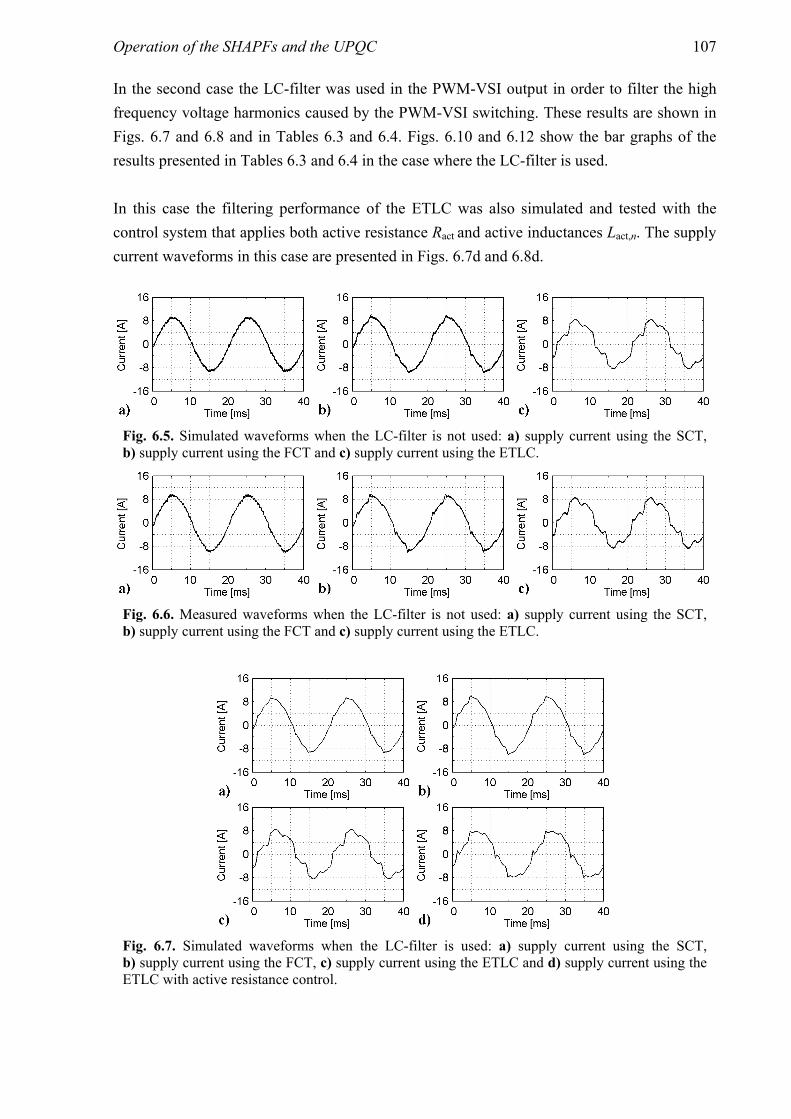
Operation of the SHAPFs and the UPQC 107
In the second case the LC-filter was used in the PWM-VSI output in order to filter the high frequency voltage harmonics caused by the PWM-VSI switching. These results are shown in Figs. 6.7 and 6.8 and in Tables 6.3 and 6.4. Figs. 6.10 and 6.12 show the bar graphs of the results presented in Tables 6.3 and 6.4 in the case where the LC-filter is used. In this case the filtering performance of the ETLC was also simulated and tested with the control system that applies both active resistance Ract and active inductances Lact,n. The supply current waveforms in this case are presented in Figs. 6.7d and 6.8d.
Fig. 6.5. Simulated waveforms when the LC-filter is not used: a) supply current using the SCT, b) supply current using the FCT and c) supply current using the ETLC.
Fig. 6.6. Measured waveforms when the LC-filter is not used: a) supply current using the SCT, b) supply current using the FCT and c) supply current using the ETLC.
Fig. 6.7. Simulated waveforms when the LC-filter is used: a) supply current using the SCT, b) supply current using the FCT, c) supply current using the ETLC and d) supply current using the ETLC with active resistance control.

108 Chapter 6
Fig. 6.8. Measured waveforms when the LC-filter is used: a) supply current using the SCT, b) supply current using the FCT, c) supply current using the ETLC and d) supply current using the ETLC with active resistance control.
Table 6.3. Simulated current harmonics filtering performance of the SHAPFs.
SCT FCT ETLC SCT FCT ETLC ETLC +Ra
LC-filter Not used Used udc [V] 700 696 699 692 683 693 682 Ract [Ω] 74 28 0 47 22 0 16
Lact,5 [mH] - - 5.2 - - 5.2 5.2 Lact,7 [mH] - - -4.4 - - -4.4 -4.4
n n
n
ii
A,lo
A,supˆˆ
[%]n
n
ii
A,lo
A,supˆˆ
[%] n
n
ii
A,lo
A,supˆˆ
[%] n
n
ii
A,lo
A,supˆˆ
[%] n
n
ii
A,lo
A,supˆˆ
[%] n
n
ii
A,lo
A,supˆˆ
[%] n
n
ii
A,lo
A,supˆˆ
[%]
1 116.4 117.2 100.2 116.4 120.0 100.7 101.7 5 7.0 18.5 62.8 12.0 24.6 64.5 34.8 7 3.9 11.1 35.6 7.2 15.7 39.4 25.1
11 26.8 52.7 77.6 39.0 58.6 78.1 86.1 13 22.4 45.1 76.8 33.2 52.4 80.3 88.7 17 22.6 48.5 83.9 33.4 54.3 80.8 90.9 19 21.4 48.8 83.8 32.3 52.3 81.6 91.3 23 33.8 67.6 80.9 45.8 62.1 82.8 91.8 25 28.9 56.1 91.1 43.3 51.4 83.2 93.0 29 51.9 58.6 77.4 62.2 50.0 80.7 89.9 31 34.4 43.4 89.0 62.2 46.9 82.1 92.1 35 194.7 48.8 84.2 115.6 52.1 80.9 88.6 37 136.0 24.3 89.5 62.1 27.1 82.5 91.0 41 145.9 27.7 88.6 72.9 28.8 81.1 88.0 43 84.6 33.0 73.7 53.9 27.0 83.8 91.6 47 63.8 37.6 70.3 51.5 31.8 80.5 87.2 49 40.2 37.1 42.8 37.3 36.4 83.9 86.7
THD2.5kHz [%] 2.8 5.4 16.4 3.8 6.5 16.7 11.3 THD20kHz [%] 2.9 5.5 16.4 3.8 6.5 16.7 11.3

Operation of the SHAPFs and the UPQC 109
Fig. 6.9. Simulated current harmonics filtering performance of the SHAPFs when the LC-filter is not used: SCT (black), FCT (grey) and ETLC (white).
Fig. 6.10. Simulated current harmonics filtering performance of the SHAPFs when the LC-filter is used: SCT (black), FCT (dark grey), ETLC (light grey) and ETLC with active resistance control (white).
Table 6.4. Measured current harmonics filtering performance of the SHAPFs.
SCT FCT ETLC SCT FCT ETLC ETLC +Ra
LC-filter Not used Used udc [V] 703 696 692 700 693 695 690 Ract [Ω] 74 28 0 47 22 0 16
Lact,5 [mH] - - 5.2 - - 5.2 5.2 Lact,7 [mH] - - -4.4 - - -4.4 -4.4
n n
n
ii
A,lo
A,supˆˆ
[%] n
n
ii
A,lo
A,supˆˆ
[%] n
n
ii
A,lo
A,supˆˆ
[%] n
n
ii
A,lo
A,supˆˆ
[%] n
n
ii
A,lo
A,supˆˆ
[%] n
n
ii
A,lo
A,supˆˆ
[%] n
n
ii
A,lo
A,supˆˆ
[%]
1 119.8 113.4 100.2 119.4 114.2 100.9 99.95 12.3 26.7 63.8 15.9 33.2 60.0 30.3 7 5.4 12.4 26.7 7.9 15.0 31.2 5.7
11 21.2 46.9 80.6 29.7 55.4 80.4 88.9 13 21.9 40.5 72.9 32.0 52.2 72.1 79.3 17 26.9 65.7 73.3 45.9 76.2 73.7 91.6 19 29.3 62.9 70.2 48.4 72.2 69.2 80.1 23 40.0 98.8 78.1 101.5 103.9 78.0 94.9 25 48.9 99.2 71.0 121.3 91.1 69.4 83.1 29 50.9 134.1 97.3 168.1 101.2 94.5 114.2 31 71.1 104.6 73.1 127.3 102.3 84.0 74.1 35 421.0 83.6 96.2 92.7 73.4 98.2 100.8 37 76.5 59.3 76.8 45.6 61.3 83.3 90.0 41 114.0 74.8 85.1 63.4 81.0 83.5 99.8 43 73.3 44.4 113.9 53.8 112.2 107.5 107.3 47 43.9 51.6 113.1 33.0 60.7 76.9 74.0 49 61.7 60.8 104.0 49.0 66.9 91.0 103.9
THD2.5kHz [%] 3.8 7.1 16.4 4.7 8.5 15.6 11.0 THD20kHz [%] 4.0 7.2 16.4 4.8 8.6 15.6 11.0
η [%] 94.5 95.2 96.1 94.1 94.8 96.3
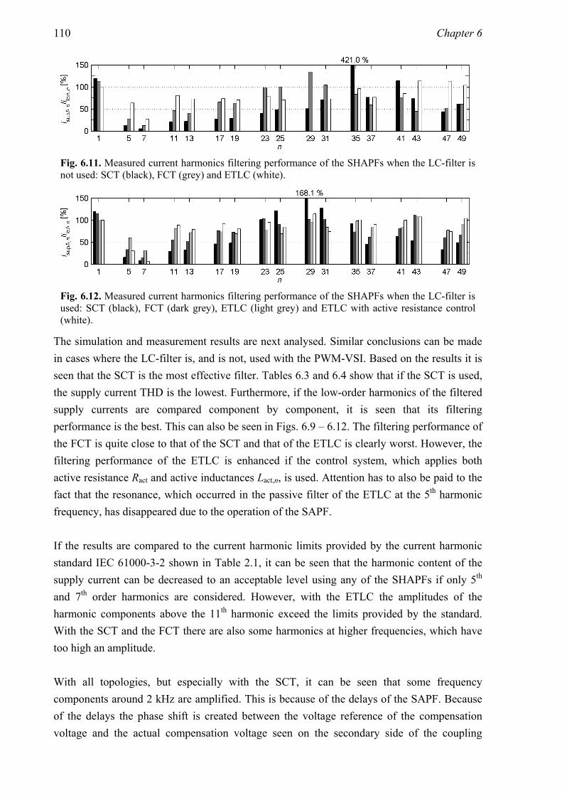
110 Chapter 6
Fig. 6.11. Measured current harmonics filtering performance of the SHAPFs when the LC-filter is not used: SCT (black), FCT (grey) and ETLC (white).
Fig. 6.12. Measured current harmonics filtering performance of the SHAPFs when the LC-filter is used: SCT (black), FCT (dark grey), ETLC (light grey) and ETLC with active resistance control (white).
The simulation and measurement results are next analysed. Similar conclusions can be made in cases where the LC-filter is, and is not, used with the PWM-VSI. Based on the results it is seen that the SCT is the most effective filter. Tables 6.3 and 6.4 show that if the SCT is used, the supply current THD is the lowest. Furthermore, if the low-order harmonics of the filtered supply currents are compared component by component, it is seen that its filtering performance is the best. This can also be seen in Figs. 6.9 – 6.12. The filtering performance of the FCT is quite close to that of the SCT and that of the ETLC is clearly worst. However, the filtering performance of the ETLC is enhanced if the control system, which applies both active resistance Ract and active inductances Lact,n, is used. Attention has to also be paid to the fact that the resonance, which occurred in the passive filter of the ETLC at the 5th harmonic frequency, has disappeared due to the operation of the SAPF. If the results are compared to the current harmonic limits provided by the current harmonic standard IEC 61000-3-2 shown in Table 2.1, it can be seen that the harmonic content of the supply current can be decreased to an acceptable level using any of the SHAPFs if only 5th and 7th order harmonics are considered. However, with the ETLC the amplitudes of the harmonic components above the 11th harmonic exceed the limits provided by the standard. With the SCT and the FCT there are also some harmonics at higher frequencies, which have too high an amplitude. With all topologies, but especially with the SCT, it can be seen that some frequency components around 2 kHz are amplified. This is because of the delays of the SAPF. Because of the delays the phase shift is created between the voltage reference of the compensation voltage and the actual compensation voltage seen on the secondary side of the coupling

Operation of the SHAPFs and the UPQC 111
transformer. With the SCT, the compensation voltage should be in the same phase with the supply current in the ideal case. However, since there is a phase delay in the compensation voltage, the compensation voltage may be at the opposite phase compared to the supply current at high frequencies and therefore these frequency components are amplified. The current at amplified frequencies flows in the high-pass filter since its impedance is low at high frequencies. This resonance is the reason for using the modulation index values lower than 0.66, as was discussed in the beginning of this chapter.
Comparison of the results with the theory
Based on these results it can be stated that the functioning principle of the SCT and FCT is more effective than that of the ETLC, i.e. the functioning principle, which is based on application of the active resistance is more effective than one that is based on the application of the active inductances. This can also be proved analytically by comparing (3.45), (3.61) and (3.74). In (3.45) and (3.61) it is seen that the increasing of the active resistance Ract decreases the amount of the supply current harmonics to an unlimited degree. However, in (3.74) it is seen that the best filtering result using the ETLC is limited by the main circuit impedances if the active resistance control is not used with it. The best filtering result is achieved in the case where the reactances Xact,n caused by the active inductances Lact,n are opposite and equal to the reactances of the LC shunt circuit Xf,n at each harmonic frequency. In this case the reactances of the nominator of (3.74) are cancelled out and it is seen that the best possible filtering result of the ETLC is limited by the ratio of the LC shunt circuit resistance and the supply impedance. The difference in the filtering performances of the SCT and FCT is caused by the different placing of the SAPF in the main circuit. Because of this different placing, the dc-link voltage control has a different influence on the current harmonics filtering performance of the SCT than that of the FCT. The influence of the dc-link voltage control on the current harmonics filtering performances of the SCT and FCT was analysed in Sections 3.4.2 and 3.5.2, respectively. As was shown in (3.49), the SAPF has to draw real power at the fundamental frequency from the supply in order to maintain the dc-link voltage. In the FCT, the SAPF is placed in series with the LC shunt circuits. Because of this, lower current at the fundamental frequency flows through the SAPF in the case of the FCT than in the case of the SCT, i.e. isupd,fu in (3.59) is higher than ifq,fu in (3.68). Besides, the nominator of the d-component of (3.59) is always smaller than that of the q-component of (3.68), because the real power flow at the harmonic frequencies is negligible in the case of the FCT, i.e. ph,dc ≈ 0. This means that to gain the same real power flow, higher voltage at the fundamental frequency has to be applied using the PWM-VSI with the FCT than with the SCT. Since the amplitude of the output voltage produced by the PWM-VSI at the fundamental frequency is higher with the FCT, less voltage

112 Chapter 6
capacity is available for the current harmonics filtering.
Influence of the LC-filter
If then the simulation and measurement results are compared in cases where the LC-filter is, and is not, used in the PWM-VSI output, the following conclusions can be made. It is seen that the supply current THD is higher in the case where the LC-filter is used. In addition to this, if the values of the active resistance Ract are considered, it is seen that Ract has lower values when the LC-filter is used. The reason for these issues is the impedances of the LC-filter, which distorts the compensation voltage. Because of the impedances of the LC-filter, the primary side voltage of the coupling transformer is not the same as the output voltage of the PWM-VSI. Because of this, the compensation voltage seen on the secondary side of the coupling transformer is lower and the filtering performance of the SHAPF worse when the LC-filter is used. Since the filtering performance of the SHAPF is worse, the harmonic content of the supply current is higher, and due to this, in (3.59) and (3.68) it is seen that the value of the active resistance Ract has to be lower if the same modulation index is used. However, it has to be noticed that the purpose of the LC-filter is not to decrease the amount of low-order harmonics of the supply current but to decrease the amount of harmonics of the compensation voltage at the switching frequency.
Efficiencies
The efficiencies of the SHAPFs in the given operating points are given in the last row of Table 6.4. The efficiencies were calculated based on the oscilloscope measurements of the phase-A load and supply current and voltage. Based on the results the efficiencies of all SHAPFs are almost the same and close to 95 %. It seems that the efficiency of the ETLC is highest and that of the SCT lowest. This would be an expected result since the SCT and the FCT have more passive filters than the ETLC and the fundamental component of the current which flows through the passive filters and the SAPF is highest with the SCT. However, the efficiencies are so close to each other that a definite answer is hard to give because the efficiencies were calculated based on the oscilloscope measurements. For example, the amount of error caused by the quantisation of the oscilloscope is in the order of 2 percentage units. If the efficiencies are compared to the efficiencies of the pure passive filters presented in Table 6.2, it can be seen that the efficiency of the SAPF is very high in each case. This is because the transformation ratio of the coupling transformer is 10:1 and very low current flows on the primary side (i.e. on the inverter side) of the transformer and through the SAPF. With the ETLC the efficiency can not be compared to the case where the pure passive filter was used because the resonance at the 5th harmonic frequency distorts the calculations.
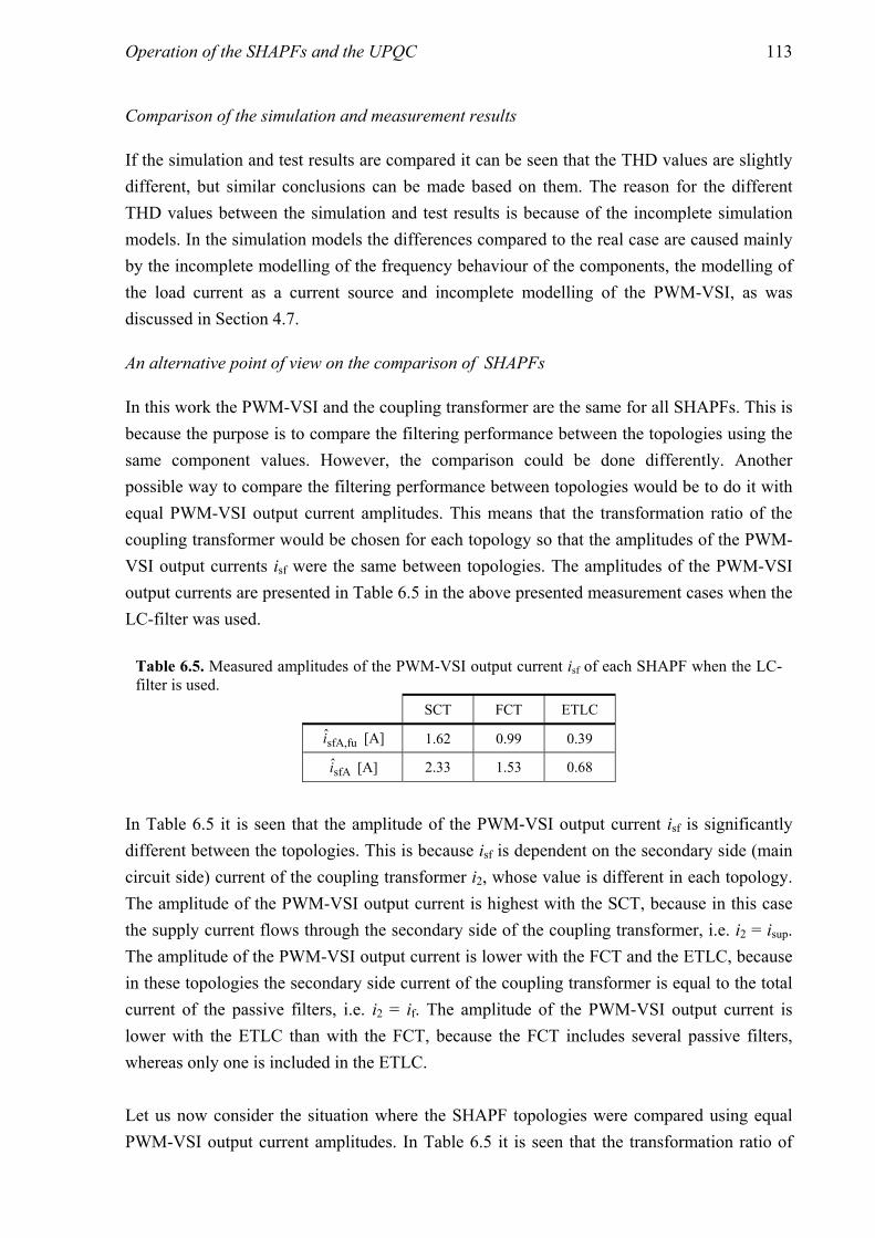
Operation of the SHAPFs and the UPQC 113
Comparison of the simulation and measurement results
If the simulation and test results are compared it can be seen that the THD values are slightly different, but similar conclusions can be made based on them. The reason for the different THD values between the simulation and test results is because of the incomplete simulation models. In the simulation models the differences compared to the real case are caused mainly by the incomplete modelling of the frequency behaviour of the components, the modelling of the load current as a current source and incomplete modelling of the PWM-VSI, as was discussed in Section 4.7.
An alternative point of view on the comparison of SHAPFs
In this work the PWM-VSI and the coupling transformer are the same for all SHAPFs. This is because the purpose is to compare the filtering performance between the topologies using the same component values. However, the comparison could be done differently. Another possible way to compare the filtering performance between topologies would be to do it with equal PWM-VSI output current amplitudes. This means that the transformation ratio of the coupling transformer would be chosen for each topology so that the amplitudes of the PWM-VSI output currents isf were the same between topologies. The amplitudes of the PWM-VSI output currents are presented in Table 6.5 in the above presented measurement cases when the LC-filter was used.
Table 6.5. Measured amplitudes of the PWM-VSI output current isf of each SHAPF when the LC-filter is used.
SCT FCT ETLC
fusfA,i [A] 1.62 0.99 0.39
sfAi [A] 2.33 1.53 0.68
In Table 6.5 it is seen that the amplitude of the PWM-VSI output current isf is significantly different between the topologies. This is because isf is dependent on the secondary side (main circuit side) current of the coupling transformer i2, whose value is different in each topology. The amplitude of the PWM-VSI output current is highest with the SCT, because in this case the supply current flows through the secondary side of the coupling transformer, i.e. i2 = isup. The amplitude of the PWM-VSI output current is lower with the FCT and the ETLC, because in these topologies the secondary side current of the coupling transformer is equal to the total current of the passive filters, i.e. i2 = if. The amplitude of the PWM-VSI output current is lower with the ETLC than with the FCT, because the FCT includes several passive filters, whereas only one is included in the ETLC. Let us now consider the situation where the SHAPF topologies were compared using equal PWM-VSI output current amplitudes. In Table 6.5 it is seen that the transformation ratio of

114 Chapter 6
the coupling transformer could be divided by the factor 1.5 in the case of the FCT and by the factor 3.4 with the ETLC in order to achieve the same amplitude of the PWM-VSI output current isf with all topologies. This division of the transformation ratio of the coupling transformer would increase the compensation voltage u2 seen on the secondary side (main circuit side) of the transformer. Because of this, the active resistance Ract would be increased in the case of the FCT. This would, of course, improve the filtering performance of the FCT. On the other hand, if the transformation ratio of the coupling transformer was decreased and the active resistance Ract not changed, the needed PWM-VSI output voltage usf would be lower. Since the necessary PWM-VSI output voltage was lower, also the dc-link voltage could be decreased. Because of this, the voltage stresses of the switching components of the PWM-VSI would be lower in this case with the FCT compared to the SCT. However, in the case of the ETLC, where only the active reactances Xact,n are produced, the changing of the transformation ratio would not have any influence on the filtering performance. This is because with the ETLC the purpose is not to maximise the output voltage of the PWM-VSI, but to produce a certain output voltage in order to produce the certain active reactances Xact,n. However, if the active resistance Ract was also applied with the ETLC, the situation would be the same, as was previously discussed with the FCT, and therefore also the current harmonics filtering performance of the ETLC would be improved in this case. On the other hand, by lowering the transformation ratio of the coupling transformer the voltage stresses of the switching components of the PWM-VSI could also be lowered in the case of the ETLC similarly as with the FCT. As was shown, the component values of the SAPF have a significant influence on the filtering performance of the SHAPF. The performance is mainly determined by the transformation ratio of the coupling transformer and the current and voltage ratings of the switching components of the PWM-VSI.
Current harmonics filtering performance with uncontrolled dc-link voltage
In this case the filtering performances of the SCT and the FCT were compared in the case where the dc-link voltage controller was not used to maintain the dc-link voltage. The dc-link voltage was maintained using a three-phase diode rectifier. The simulations and measurements were performed using two dc-link voltage levels. In the first case, the dc-link voltage was maintained using the three-phase diode rectifier connected directly to the power supply. In this case the dc-link voltage was approximately 560 V. In the second case the dc-link voltage was also maintained using the three-phase diode rectifier, but here the input voltage of the diode rectifier was increased using a three-phase transformer so that the dc-link voltage was increased to approximately 700 V. The LC-filter was used in these simulations and tests. The results are presented in Figs. 6.13 – 6.16 and in Tables 6.6 and 6.7.

Operation of the SHAPFs and the UPQC 115
Fig. 6.13. Simulated waveforms using dc-link voltage 560 V: a) supply current using the SCT and b) supply current using the FCT.
Fig. 6.14. Measured waveforms using dc-link voltage 560 V: a) supply current using the SCT and b) supply current using the FCT.
Fig. 6.15. Simulated waveforms using dc-link voltage 700 V: a) supply current using the SCT and b) supply current using the FCT.
Fig. 6.16. Measured waveforms using dc-link voltage 700 V: a) supply current using SCT and b) supply current using the FCT.

116 Chapter 6
Table 6.6. Simulated current harmonics filtering performance of the SHAPFs.
SCT FCT SCT FCT udc [V] 563 565 699 696
Ract 24 20 50 30
n n
n
ii
A,lo
A,supˆˆ
[%]n
n
ii
A,lo
A,supˆˆ
[%]n
n
ii
A,lo
A,supˆˆ
[%]n
n
ii
A,lo
A,supˆˆ
[%]
1 116.5 116.5 116.5 116.55 21.5 25.8 11.5 18.8 7 13.3 16.1 6.8 11.4
11 56.5 60.8 37.4 50.8 13 49.8 54.1 31.7 43.8 17 52.0 56.0 31.8 45.2 19 52.7 54.7 31.8 44.7 23 63.3 62.7 45.5 60.7 25 52.2 52.5 42.2 53.5 29 51.1 47.3 54.4 63.6 31 42.4 39.4 60.9 49.0 35 52.1 45.8 150.8 65.6 37 24.3 26.6 71.3 30.0 41 32.1 32.9 56.9 36.7 43 34.2 28.6 54.3 47.4 47 35.7 28.2 44.6 46.0 49 32.7 25.7 45.2 27.5
THD2.5kHz [%] 6.1 6.9 3.7 5.4 THD20kHz [%] 6.1 6.9 3.7 5.4
Table 6.7. Measured current harmonics filtering performance of the SHAPFs.
SCT FCT SCT FCT udc [V] 563 565 699 696
Ract 24 20 50 30
n n
n
ii
A,lo
A,supˆˆ
[%] n
n
ii
A,lo
A,supˆˆ
[%]n
n
ii
A,lo
A,supˆˆ
[%]n
n
ii
A,lo
A,supˆˆ
[%]
1 118.3 113.5 118.0 113.05 27.6 34.2 13.8 25.6 7 13.6 15.1 6.9 10.3
11 47.6 56.3 27.9 46.4 13 52.1 52.9 29.6 44.4 17 68.1 72.8 42.4 71.3 19 66.6 69.7 40.0 73.8 23 88.2 94.3 95.2 114.8 25 87.4 81.8 109.9 116.7 29 85.4 105.7 196.3 135.1 31 80.3 104.4 146.7 107.7 35 63.8 69.3 84.1 88.7 37 27.3 53.8 49.7 79.7 41 53.5 65.9 69.5 68.2 43 53.4 92.6 61.2 78.3 47 27.3 43.9 47.6 49.4 49 43.4 70.2 46.1 70.9
THD2.5kHz [%] 7.1 8.7 4.4 7.2 THD20kHz [%] 7.1 8.7 4.5 7.2
Operation of the SHAPFs and the UPQC 117
Several facts are seen based on the simulation and measurement results. First of all, in Tables 6.6 and 6.7 it can be seen that the increasing of the dc-link voltage improves the current harmonics filtering performance of both SCT and FCT. This is because the higher dc-link voltage enables the use of higher active resistance Ract. This was shown analytically in (3.46) and (3.47).
Comparison of the results between different dc-link voltage maintenance methods
If the results achieved using the dc-link voltage 700 V are compared to the results of the previous case, where this same dc-link voltage was maintained using the dc-link voltage control, it can be seen that the filtering performances of the SHAPFs are better in this case, where the dc-link is maintained using the diode rectifier. Also the active resistances are slightly higher in this case. The reason for these can be seen in (3.59) and (3.68). Since the dc-link voltage is maintained using an auxiliary power supply, there is no fundamental component in the output voltage of the PWM-VSI. Since there is no fundamental component, the whole voltage capacity can be used in current harmonics filtering, i.e. the active resistance Ract can be increased and the filtering performance enhanced with both topologies.
Influence of the dc-link control on the current harmonics performance of the SHAPFs
When the dc-link voltage was maintained by using the dc-link voltage control, it was noticed that the current harmonics filtering performance of the FCT was worse than that of the SCT. However, if that case is compared to one, where the same dc-link voltage is maintained using the diode rectifier, it can be seen that the current harmonics filtering performance of the FCT is more enhanced and therefore the current harmonics filtering performances of the SCT and the FCT are closer to each other. The same can also be seen in the active resistances: Ract can be increased more in the case of FCT than that of the SCT and therefore the active resistance values between the SCT and the FCT are closer to each other when the dc-link voltage is maintained using the diode rectifier. Because of the reasons mentioned in Section 3.5.2, the fundamental component of the output voltage of the PWM-VSI is higher in the case of FCT than in the case of the SCT if the dc-link voltage is maintained using the dc-link control. When the dc-link voltage is maintained using the diode rectifier, this fundamental component is equal to zero and therefore the output voltage capacity, which can be used for harmonics filtering, is more increased in the case of the FCT. Therefore it can be concluded that the dc-link voltage control has more influence on the filtering performance of the FCT than that of the SCT.
Comparison of the simulation and measurement results
If the simulation and measurement results are compared, it can be seen that they differ. The reasons for the different THD values between the simulation and test results are imperfections

118 Chapter 6
of the simulation models, which were discussed in Section 4.7. However, based on the results of the simulations and experimental tests, similar conclusions can be made.
6.1.2 RC-type nonlinear load
This subchapter presents the simulation and measurement results using the RC-type nonlinear load. The current harmonics filtering performance of the SHAPFs was simulated and tested in similar cases as was presented previously in the case of the RL-type nonlinear load.
Current harmonics filtering performance of the passive filters
The current harmonics filtering performance of the passive filters of the SHAPFs was simulated and tested first. In this case the SAPF was not connected to the main circuit. The results of the simulations and tests are presented in Figs. 6.17 and 6.18 and in Tables 6.8 and 6.9. The current harmonics filtering performances of the passive filters presented in Tables 6.8 and 6.9 are also presented as bar graphs in Figs. 6.19 and 6.20.
Fig. 6.17. Simulated waveforms: a) load current, b) supply current in the case of the SCT and FCT and c) supply current in the case of the ETLC.
Fig. 6.18. Measured waveforms: a) load current, b) supply current in the case of the SCT and FCT and c) supply current in the case of the ETLC.

Operation of the SHAPFs and the UPQC 119
Table 6.8. Simulated current harmonics filtering performance of the passive filters.
Load SCT FCT ETLC
n ni A,loˆ [A] n
n
ii
A,lo
A,supˆˆ
[%]n
n
ii
A,lo
A,supˆˆ
[%]
1 7.81 111.0 98.05 2.94 64.9 128.7 7 0.97 34.8 67.8
11 0.54 86.5 77.4 13 0.26 91.3 80.7 17 0.21 77.1 79.7 19 0.16 61.7 82.0 23 0.10 51.6 83.9 25 0.09 44.5 80.2 29 0.06 30.2 79.9 31 0.07 42.3 82.5 35 0.03 46.5 80.8 37 0.04 24.4 83.8 41 0.04 27.0 82.5 43 0.03 43.2 79.3 47 0.03 22.7 79.2 49 0.02 30.6 83.6
THD20kHz [%] 40.7 23.3 50.7
Table 6.9. Measured current harmonics filtering performance of the passive filters.
Load SCT FCT ETLC
n ni A,loˆ [A] n
n
ii
A,lo
A,supˆˆ
[%] n
n
ii
A,lo
A,supˆˆ
[%]
1 7.81 114.4 98.15 2.94 71.2 140.7 7 0.97 52.1 19.9
11 0.54 59.5 70.5 13 0.27 41.5 71.0 17 0.21 58.2 71.5 19 0.16 38.2 75.8 23 0.10 61.7 74.4 25 0.09 36.6 72.6 29 0.05 60.7 86.2 31 0.06 52.2 61.7 35 0.04 25.7 77.6 37 0.04 34.6 58.0 41 0.04 43.7 81.9 43 0.03 39.3 98.3 47 0.03 14.6 75.5 49 0.03 25.0 66.3
THD20kHz [%] 40.7 24.5 54.5 η [%] 94.9 94.8
Fig. 6.19. Simulated current harmonics filtering performance of the passive filters: SCT/FCT (black) and ETLC (white).
Fig. 6.20. Measured current harmonics filtering performance of the passive filters: SCT/FCT (black) and ETLC (white).
Based on these results, similar conclusions can be made as in the case of the RL-type nonlinear load. It can be seen that the current harmonics are decreased due to the use of the passive filters of the SCT/FCT. However, in the case of the passive filter of the ETLC it can

120 Chapter 6
be seen that there is a resonance at the 5th harmonic component. This was also seen with the RL-type nonlinear load. If the measurement results are compared to the values provided by the standard IEC 61000-3-2 which were shown in the Table 2.1, it can be seen that the supply current harmonics are too high if any filter is not used with the load. If the passive filters are used, the situation is not changed, i.e. the supply current includes current components with too high amplitude. In the case of the ETLC the 5th harmonic current is higher than is specified in the standard because of the resonance. In the case of the passive filters of the SCT/FCT the current filtering performance of the passive filters is too low, because the amplitude of the 5th harmonic current is too high despite the passive filtering. In the results it can be seen that the simulations agree well with the measurement results. The load current waveform of the simulations is identical compared to the measurements since the measured load current waveform was used as an input of the simulation model. The supply current components are not the same between the simulations and the measurements because of the defects of the simulation models, which were discussed in Section 4.7.
Current harmonics filtering performance of the SHAPFs
Next, the simulation and measurement results, where the SAPF was connected to the main circuit of the SHAPFs, are presented. The simulations and tests were performed similarly as in the case of the RL-type nonlinear load. First, the current harmonics filtering performance of the SHAPFs is inspected in the case where the LC-filter is not connected to the output of the PWM-VSI. After this the simulation and test results using the LC-filter are shown. The current harmonics filtering performance of the ETLC is simulated and tested with and without active resistance control. The results are presented in Figs. 6.21 – 6.24 and in Tables 6.10 and 6.11. The current harmonics filtering performances of the SHAPFs presented in Tables 6.10 and 6.11 are also shown as bar graphs in Figs. 6.25 – 6.28.
Fig. 6.21. Simulated waveforms when the LC-filter is not used: a) supply current using the SCT, b) supply current using the FCT and c) supply current using the ETLC.

Operation of the SHAPFs and the UPQC 121
Fig. 6.22. Measured waveforms when the LC-filter is not used: a) supply current using the SCT, b) supply current using the FCT and c) supply current using the ETLC.
Fig. 6.23. Simulated waveforms when the LC-filter is used: a) supply current using the SCT, b) supply current using the FCT, c) supply current using the ETLC and d) supply current using the ETLC with active resistance control.
Fig. 6.24. Measured waveforms when the LC-filter is used: a) supply current using the SCT, b) supply current using the FCT, c) supply current using the ETLC and d) supply current using the ETLC with active resistance control.
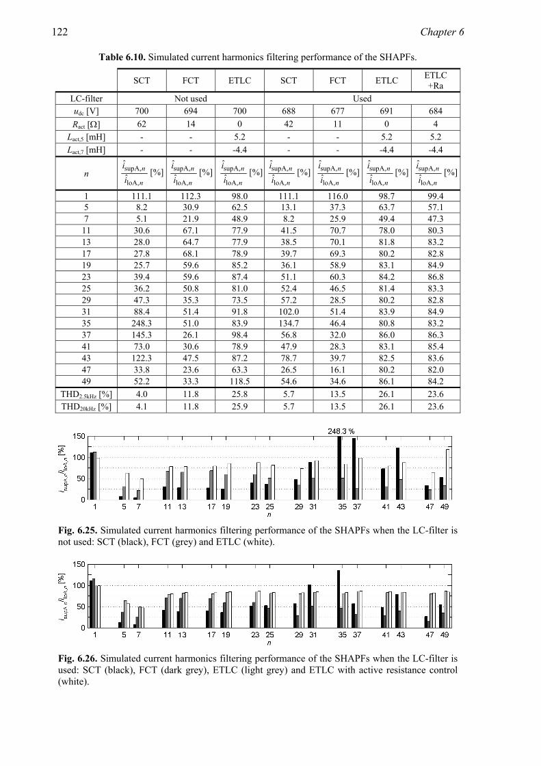
122 Chapter 6
Table 6.10. Simulated current harmonics filtering performance of the SHAPFs.
SCT FCT ETLC SCT FCT ETLC ETLC +Ra
LC-filter Not used Used udc [V] 700 694 700 688 677 691 684 Ract [Ω] 62 14 0 42 11 0 4
Lact,5 [mH] - - 5.2 - - 5.2 5.2 Lact,7 [mH] - - -4.4 - - -4.4 -4.4
n n
n
ii
A,lo
A,supˆˆ
[%]n
n
ii
A,lo
A,supˆˆ
[%] n
n
ii
A,lo
A,supˆˆ
[%]n
n
ii
A,lo
A,supˆˆ
[%]n
n
ii
A,lo
A,supˆˆ
[%]n
n
ii
A,lo
A,supˆˆ
[%] n
n
ii
A,lo
A,supˆˆ
[%]
1 111.1 112.3 98.0 111.1 116.0 98.7 99.4 5 8.2 30.9 62.5 13.1 37.3 63.7 57.1 7 5.1 21.9 48.9 8.2 25.9 49.4 47.3
11 30.6 67.1 77.9 41.5 70.7 78.0 80.3 13 28.0 64.7 77.9 38.5 70.1 81.8 83.2 17 27.8 68.1 78.9 39.7 69.3 80.2 82.8 19 25.7 59.6 85.2 36.1 58.9 83.1 84.9 23 39.4 59.6 87.4 51.1 60.3 84.2 86.8 25 36.2 50.8 81.0 52.4 46.5 81.4 83.3 29 47.3 35.3 73.5 57.2 28.5 80.2 82.8 31 88.4 51.4 91.8 102.0 51.4 83.9 84.9 35 248.3 51.0 83.9 134.7 46.4 80.8 83.2 37 145.3 26.1 98.4 56.8 32.0 86.0 86.3 41 73.0 30.6 78.9 47.9 28.3 83.1 85.4 43 122.3 47.5 87.2 78.7 39.7 82.5 83.6 47 33.8 23.6 63.3 26.5 16.1 80.2 82.0 49 52.2 33.3 118.5 54.6 34.6 86.1 84.2
THD2.5kHz [%] 4.0 11.8 25.8 5.7 13.5 26.1 23.6 THD20kHz [%] 4.1 11.8 25.9 5.7 13.5 26.1 23.6
Fig. 6.25. Simulated current harmonics filtering performance of the SHAPFs when the LC-filter is not used: SCT (black), FCT (grey) and ETLC (white).
Fig. 6.26. Simulated current harmonics filtering performance of the SHAPFs when the LC-filter is used: SCT (black), FCT (dark grey), ETLC (light grey) and ETLC with active resistance control (white).

Operation of the SHAPFs and the UPQC 123
Table 6.11. Measured current harmonics filtering performance of the SHAPFs.
SCT FCT ETLC SCT FCT ETLC ETLC +Ra
LC-filter Not used Used udc [V] 702 689 695 697 686 696 690 Ract [Ω] 62 14 0 42 11 0 4
Lact,5 [mH] - - 5.2 - - 5.2 5.2 Lact,7 [mH] - - -4.4 - - -4.4 -4.4
n n
n
ii
A,lo
A,supˆˆ
[%] n
n
ii
A,lo
A,supˆˆ
[%]n
n
ii
A,lo
A,supˆˆ
[%]n
n
ii
A,lo
A,supˆˆ
[%]n
n
ii
A,lo
A,supˆˆ
[%] n
n
ii
A,lo
A,supˆˆ
[%] n
n
ii
A,lo
A,supˆˆ
[%]
1 116.9 108.1 97.1 116.6 109.2 96.9 96.85 11.8 44.4 66.1 13.5 51.2 65.7 61.5 7 6.0 49.1 47.2 6.4 54.4 55.2 61.1
11 17.7 57.2 75.4 24.7 61.4 74.7 80.4 13 11.0 71.1 61.2 12.2 67.2 63.7 58.9 17 36.4 73.2 78.7 53.3 70.3 82.9 94.3 19 22.2 61.1 60.3 27.5 59.3 64.4 74.3 23 71.6 79.4 95.3 117.2 84.5 94.4 105.1 25 60.8 62.3 71.2 70.4 66.7 75.1 81.9 29 143.0 67.1 102.4 144.4 72.5 84.7 92.4 31 171.0 55.1 73.0 90.7 57.2 78.6 78.8 35 116.1 55.7 68.6 62.3 58.3 63.5 73.3 37 111.3 55.8 73.5 72.9 54.2 71.9 72.7 41 54.5 27.6 52.4 73.5 39.2 59.3 84.5 43 79.9 65.2 76.1 49.3 53.5 73.2 92.8 47 12.4 41.6 82.0 31.6 53.4 76.2 78.0 49 40.1 46.2 55.0 31.2 24.8 47.0 65.2
THD2.5kHz [%] 4.7 17.2 27.3 5.4 19.4 27.4 26.3 THD20kHz [%] 4.9 17.3 27.3 5.4 19.5 27.5 26.3
η [%] 93.7 94.5 95.4 92.8 93.6 95.6
Fig. 6.27. Measured current harmonics filtering performance of the SHAPFs when the LC-filter is not used: SCT (black), FCT (grey) and ETLC (white).
Fig. 6.28. Measured current harmonics filtering performance of the SHAPFs when the LC-filter is used: SCT (black), FCT (dark grey), ETLC (light grey) and ETLC with active resistance control (white).
124 Chapter 6
In this case, where the RC-type non-linear load is used, similar conclusions can be made as in the case of the RL-type non-linear load. Based on the results it can be seen that the current harmonics filtering performance of the SCT is the best and that of the ETLC is the worst. In this case the current harmonics filtering performance of the SCT is clearly better than that of the FCT or the ETLC. The current harmonics filtering result of the ETLC is improved by the use of the control system which applies both active resistance Ract and the active inductances Lact,n. In the case of the ETLC the use of the SAPF removes the resonance of the LC shunt circuit, which occurs at the 5th harmonic frequency. The results are next compared to the current harmonic limits of the current harmonic standard IEC 61000-3-2, which were shown in Table 2.1. It can be seen that the current harmonics requirements of the standard are approximately fulfilled only in the case of the SCT. The requirements are not fulfilled exactly, since there are some harmonic components at the higher frequencies, which exceed the limits specified in the standard. The inspection of the efficiencies of the SHAPFs in the given operation points, which are presented in the last row of Table 6.11, gives similar results to the case of the RL-type nonlinear load. The efficiencies of the topologies are very close to each other: close to 95 %. Also the order of the topologies is the same: the efficiency of the ETLC is the highest and the efficiency of the SCT lowest. However, it has to be again remembered that the differences between the efficiencies are smaller than the possible error caused by the measurement. Although the test results do not totally agree with the simulation results, similar conclusions can be made based on both of these. It can be seen that the differences between the results are largest in the case of the FCT. The reason for the differences between the simulation and test results is the incompleteness of the simulation models. This issue was discussed in Section 4.7. In this case, where the RC-type nonlinear load is used, the error in the simulation results is caused especially because of the modelling of the load current as a current source. In the simulations it was assumed that the load current is independent on the load voltage. However, in this case, where the load impedance is low, the fluctuations of the load voltage have an influence on the harmonic content of the load current. The dependency of the load current on the load voltage is discussed in Appendix D. In the appendix it can be seen that if the RC-type nonlinear load is used, the harmonic content of the load current changes significantly when the SAPF is connected to the main circuit of the SHAPF. The change of the harmonic content is biggest in the case of the FCT. Since the harmonic content of the load current is different in the measurements than is assumed in the simulations, also the simulated supply current differs from the measured one. Since the change of the harmonic content of the load current is highest in the case of the FCT, also its simulation result differs most with the measurement
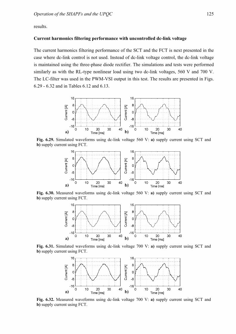
Operation of the SHAPFs and the UPQC 125
results.
Current harmonics filtering performance with uncontrolled dc-link voltage
The current harmonics filtering performance of the SCT and the FCT is next presented in the case where dc-link control is not used. Instead of dc-link voltage control, the dc-link voltage is maintained using the three-phase diode rectifier. The simulations and tests were performed similarly as with the RL-type nonlinear load using two dc-link voltages, 560 V and 700 V. The LC-filter was used in the PWM-VSI output in this test. The results are presented in Figs. 6.29 - 6.32 and in Tables 6.12 and 6.13.
Fig. 6.29. Simulated waveforms using dc-link voltage 560 V: a) supply current using SCT and b) supply current using FCT.
Fig. 6.30. Measured waveforms using dc-link voltage 560 V: a) supply current using SCT and b) supply current using FCT.
Fig. 6.31. Simulated waveforms using dc-link voltage 700 V: a) supply current using SCT and b) supply current using FCT.
Fig. 6.32. Measured waveforms using dc-link voltage 700 V: a) supply current using SCT and b) supply current using FCT.

126 Chapter 6
Table 6.12. Simulated current harmonics filtering performance of the SHAPFs.
SCT FCT SCT FCT udc [V] 555 551 697 695
Ract 30 13 47 18
n n
n
ii
A,lo
A,supˆˆ
[%]n
n
ii
A,lo
A,supˆˆ
[%] n
n
ii
A,lo
A,supˆˆ
[%]n
n
ii
A,lo
A,supˆˆ
[%]
1 111.2 111.2 111.2 111.35 17.6 33.8 11.9 27.4 7 11.1 23.6 7.3 19.2
11 50.1 67.8 38.8 62.0 13 46.9 66.7 35.0 59.4 17 51.4 67.4 36.3 61.1 19 46.3 58.1 33.1 54.7 23 61.3 60.2 46.9 64.7 25 60.2 50.3 48.0 56.9 29 51.6 28.7 57.0 35.1 31 77.7 53.7 96.1 52.9 35 86.2 50.6 161.3 53.0 37 39.9 32.8 76.3 38.4 41 34.7 27.6 59.6 30.9 43 66.7 44.8 106.0 44.6 47 31.2 22.1 37.1 18.2 49 39.4 34.9 45.6 39.5
THD2.5kHz [%] 7.3 12.9 5.2 10.6 THD20kHz [%] 7.3 12.9 5.2 10.6
Table 6.13. Measured current harmonics filtering performance of the SHAPFs.
SCT FCT SCT FCT udc [V] 555 551 697 695
Ract 30 13 47 18
n n
n
ii
A,lo
A,supˆˆ
[%]n
n
ii
A,lo
A,supˆˆ
[%]n
n
ii
A,lo
A,supˆˆ
[%]n
n
ii
A,lo
A,supˆˆ
[%]
1 117.8 112.4 116.4 113.25 19.2 45.1 12.0 36.3 7 9.6 50.1 6.5 46.1
11 33.1 58.9 22.5 53.4 13 16.8 76.6 11.6 75.0 17 71.4 76.9 49.9 77.4 19 23.2 55.2 24.4 61.2 23 114.9 87.3 117.7 101.4 25 59.7 68.9 86.8 78.0 29 103.1 89.0 200.4 105.7 31 77.2 63.8 125.0 68.5 35 46.3 66.0 88.6 69.4 37 68.1 75.5 81.0 65.2 41 70.1 75.4 83.1 67.7 43 32.9 75.9 58.3 61.4 47 41.5 41.1 35.9 52.8 49 20.6 42.7 40.8 64.6
THD2.5kHz [%] 7.1 17.0 5.1 14.0 THD20kHz [%] 7.1 17.0 5.2 14.0

Operation of the SHAPFs and the UPQC 127
Based on the results, similar conclusions can be made as in the case of the RL-type nonlinear load. It is seen that the higher dc-link voltage leads to a better current harmonics filtering result with both SCT and FCT, because the higher dc-link voltage makes possible to increase the active resistance Ract. If the results achieved using dc-link voltage 700 V are compared to the previous simulation and measurement results, where the dc-link voltage was maintained using dc-link voltage control, it can be seen that the filtering results are better when the rectifier is used to maintain the dc-link voltage. It can also be seen that the current harmonics filtering performance of the FCT is enhanced more than that of the SCT compared to the case where the dc-link control was used.
6.1.3 Stepwise changing load current
This subchapter presents the simulation and measurement results of the three SHAPFs in the case of the stepwise changing load current. The simulations and tests were performed using the same RL-type nonlinear load as in the steady-state simulations and tests. The LC-filter was used in the output of the PWM-VSI with all topologies. The dc-link voltage controller was used to maintain the dc-link voltage with each topology. The dc-link voltage reference was 700 V. The control system parameters of the SHAPFs were the same as in the steady-state tests. The parameters are shown in Table 6.14.
Table 6.14. Control system parameters.
Parameter SCT FCT ETLC Ract [Ω] 47 22
Lact,5 [mH] 5.2 Lact,7 [mH] -4.4
The stepwise changing load current was realised by changing the value of the load resistor between 72 Ω (3.8 kVA) and 212 Ω (1.3 kVA). The results are presented in Figs. 6.33 – 6.44. In Figs. 6.33 – 6.36 the simulated and measured load current and supply current of the SCT are presented in cases of increasing and decreasing load current. In Figs. 6.37 – 6.40 these same waveforms are presented in the case of the FCT and in Figs. 6.41 – 6.44 the ETLC.
Fig. 6.33. Simulated waveforms in the case of SCT: a) Load current and b) supply current.

128 Chapter 6
Fig. 6.34. Measured waveforms in the case of SCT: a) Load current and b) supply current.
Fig. 6.35. Simulated waveforms in the case of SCT: a) Load current and b) supply current.
Fig. 6.36. Measured waveforms in the case of SCT: a) Load current and b) supply current.
Fig. 6.37. Simulated waveforms in the case of FCT: a) Load current and b) supply current.
Fig. 6.38. Measured waveforms in the case of FCT: a) Load current and b) supply current.
Fig. 6.39. Simulated waveforms in the case of FCT: a) Load current and b) supply current.

Operation of the SHAPFs and the UPQC 129
Fig. 6.40. Measured waveforms in the case of FCT: a) Load current and b) supply current.
Fig. 6.41. Simulated waveforms in the case of ETLC: a) Load current and b) supply current.
Fig. 6.42. Measured waveforms in the case of ETLC: a) Load current and b) supply current.
Fig. 6.43. Simulated waveforms in the case of ETLC: a) Load current and b) supply current.
Fig. 6.44. Measured waveforms in the case of ETLC: a) Load current and b) supply current.
Based on the results it is seen that the SHAPFs also operate during the stepwise changing load current in the presented cases. It can be seen that it takes less than one fundamental period for each SHAPF to adapt to the new supply current value. However, in order to make the operation of the SAPF stable during the stepwise changing load current in the cases of the SCT and FCT, changes had to be made to their control

130 Chapter 6
systems. This is because the harmonic filtering of these topologies is based on the applying of active resistance. If the changes are not done, the change of the load current is seen by the control system as a huge amount of harmonic components, which are amplified with the gain Ract by the control system. The result of this is a high output voltage of the PWM-VSI, which leads to an overcurrent situation in the output of the PWM-VSI.
6.2 Operation of the UPQC
The operation of the UPQC is examined in this chapter through the simulations and prototype tests. The steady-state operation as well as operation during the dynamic changes is dealt with. In steady-state operation, a 2.4 kVA RL-type nonlinear load is used. The RL-type nonlinear load consists of a three-phase rectifier with inductor and resistor connected in series on its dc-side. In the prototype tests ELGAR SW 5250A linear three-phase power supply is used to produce 230/400 V (50 Hz) supply voltage. In stationary operation the current and voltage harmonics filtering performances of the UPQC are researched. The current harmonics filtering performance is first researched using sinusoidal supply voltage. After this, both current and voltage harmonics filtering performances are inspected using the distorted supply voltage. The operation of the UPQC during dynamic changes is researched in two cases. In the first case the UPQC is used in voltage dip compensation. In this case the supply voltage dips to 78 % of its nominal value and the UPQC is used to compensate for this disturbance. In the second case the operation of the UPQC during the stepwise changing load current is dealt with. In both cases the RL-type nonlinear load is used. Only the simulation and measurement results of phase-A are presented. This is because the three-phase system is symmetrical in the inspected cases and therefore equal conclusions can be made based on all phases.
Steady-state operation with sinusoidal supply voltage
In this case the aim is to filter the current harmonics, which are produced by the RL-type nonlinear load. The simulations and tests were performed with two control system configurations. In the first one the PI-control branch of the SAPF control system, which was shown in Fig. 3.21 in the case of the UPQC, was disabled. In the other one the PI-control was enabled. The results are presented in Figs. 6.45 – 6.48 and in Tables 6.15 - 6.18.
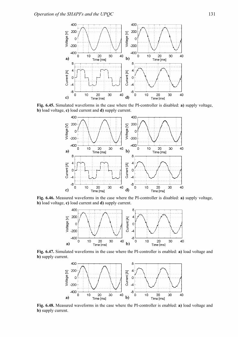
Operation of the SHAPFs and the UPQC 131
Fig. 6.45. Simulated waveforms in the case where the PI-controller is disabled: a) supply voltage, b) load voltage, c) load current and d) supply current.
Fig. 6.46. Measured waveforms in the case where the PI-controller is disabled: a) supply voltage, b) load voltage, c) load current and d) supply current.
Fig. 6.47. Simulated waveforms in the case where the PI-controller is enabled: a) load voltage and b) supply current.
Fig. 6.48. Measured waveforms in the case where the PI-controller is enabled: a) load voltage and b) supply current.

132 Chapter 6
Table 6.15. Characteristics of the simulated voltages.
Supply voltage Load voltage Load voltage
PI-control Disabled Enabled
n nu A,supˆ [V]n
nuu
,supA
A,loˆˆ
[%]n
nuu
,supA
A,loˆˆ
[%]
1 324.98 99.6 99.9THD2.5kHz [%] 0.6 2.3 2.3 THD20kHz [%] 0.9 3.2 3.2
Table 6.16. Simulated current harmonics filtering performance of the UPQC.
Load current Supply current
Supply current
PI-control Disabled Enabled
n ni A,loˆ [A] n
n
ii
A,lo
A,supˆˆ
[%]n
n
ii
A,lo
A,supˆˆ
[%]
1 4.88 109.8 109.95 1.11 3.7 4.7 7 0.54 8.4 5.1
11 0.43 24.0 22.7 13 0.27 43.4 47.7 17 0.24 74.6 77.5 19 0.17 70.6 58.4 23 0.13 53.5 49.0 25 0.11 44.1 56.1 29 0.08 39.6 34.1 31 0.07 41.3 42.4 35 0.05 32.9 33.2 37 0.04 34.9 34.3 41 0.03 43.5 40.5 43 0.03 30.9 18.7 47 0.02 27.3 26.8 49 0.02 39.1 30.5
THD2.5kHz [%] 28.4 5.5 5.4 THD20kHz [%] 28.5 5.7 5.7
Table 6.17. Characteristics of the measured voltages.
Supply voltage Load voltage Load voltage
PI-control Disabled Enabled
n nu A,supˆ [V]n
nuu
,supA
A,loˆˆ
[%]n
nuu
,supA
A,loˆˆ
[%]
1 324.81 91.3 99.7THD2.5kHz [%] 0.6 3.2 3.2 THD20kHz [%] 1.0 3.4 3.4

Operation of the SHAPFs and the UPQC 133
Table 6.18. Measured current harmonics filtering performance of the UPQC.
Load current Supply current
Supply current
PI-control Disabled Enabled
n ni A,loˆ [A] n
n
ii
A,lo
A,supˆˆ
[%]n
n
ii
A,lo
A,supˆˆ
[%]
1 4.89 96.8 113.95 1.10 19.9 18.5 7 0.55 14.0 13.1
11 0.42 29.4 33.0 13 0.28 41.2 50.0 17 0.24 31.9 47.7 19 0.17 31.4 42.8 23 0.13 23.1 38.1 25 0.11 20.1 29.0 29 0.07 20.4 23.1 31 0.07 15.2 19.4 35 0.04 17.8 18.7 37 0.05 12.9 17.5 41 0.03 15.4 35.3 43 0.03 13.6 27.0 47 0.02 11.9 16.9 49 0.02 23.7 11.9
THD2.5kHz [%] 28.2 6.7 6.2 THD20kHz [%] 28.3 6.8 6.3
Based on the results it can be stated that the UPQC filters the current harmonics efficiently. The supply current THD is almost the same in cases where the PI-control branch of the SAPF control system is disabled and enabled. This is natural, since the aim of the PI-control is not to influence on the harmonics filtering, but to correct the amplitude of the load voltage at the fundamental frequency. If the harmonic contents of the currents are compared to the current harmonics limits of the current harmonic standard IEC 61000-3-2 presented in Table 2.1, it can be seen that the amplitudes of the harmonic components of all currents are lower than the maximum values specified in the standard. If the results are examined, it can be seen that the simulation results agree well with the measurement results, although there are some differences. The supply voltage and the load current waveforms are similar in the simulations and in the measurements, because the measured waveforms were used as inputs of the simulation model. However, in the simulated supply current waveforms presented in Figs. 6.45d and 6.47b high frequency ripple can be seen. On the other hand, in the respective measured supply currents shown in Figs. 6.46d and 6.48b this ripple does not exist. In Table 6.16 it can be seen that the high frequency components, which can be seen in the simulated waveforms, occur at the 17th and 19th harmonic frequency. The reason for this difference is the incomplete modelling of the passive

134 Chapter 6
components of the LCL-filter of the parallel active power filter (PAPF). Because of this incomplete modelling, the damping of the real LCL-filter is higher than the damping of the simulated LCL-filter at the 17th and 19th harmonic frequency. The lower damping of the LCL-filter in the simulation model can be seen as higher LCL-filter current at these frequencies, and in addition to this, also as higher supply current at these frequencies. Another difference between the simulation and measurement results can be seen in Tables 6.15 - 6.18. As is seen, there are differences in the fundamental frequency components of the currents and voltages. This is because of the imperfections of the modelling of the PWM-VSI. In the simulation models, the switching bridge of the PWM-VSI was assumed to be ideal. However, in reality the output voltage of the PWM-VSI at the fundamental frequency is not zero, although its voltage reference is. This is because of the dead times between the inverter switchings. Some error is also added by the imperfect calibration of the measurement circuits of the SAPF. In the case where the PI-control is disabled in the control system of the SAPF the situation can not be corrected since the open loop control is used. Because of this the PWM-VSI output voltage reference and actual output voltage are different. Since the output voltage of the PWM-VSI influences on the load voltage, this error can also be seen in it. However, when the PI-control is enabled the error is corrected by the control system. As can be seen in Table 6.18, when the PI-control is enabled the measured fundamental frequency component of the supply current is higher than when the PI-control is disabled. This is because of the operating principle of the UPQC. Since the SAPF produces an output voltage at the fundamental frequency, energy is taken from the dc-link of the PWM-VSI. In order to compensate this energy loss and to maintain the desired dc-link voltage level, PAPF absorbs energy from the supply. Because of the operating principle of the PAPF, this can be seen as increasing of the fundamental component the PAPF output current, which is seen as an increase of the supply current at the fundamental frequency. When the PI-control is disabled, the fundamental component of the supply current is lower, and since the output voltage of the SAPF at the fundamental frequency is lower, less energy is taken from the dc-link and therefore the fundamental component of the PAPF output current is lower. The abovementioned issues can not be seen in the simulation results since the ideal model of the PWM-VSI is used. In addition to this, the efficiency of the UPQC was also calculated. When the PI-control was disabled it was 95.1 %, and when it was enabled it was 96.0 %.
Steady-state operation with distorted supply voltage
In this subchapter the steady-state filtering performance of the UPQC is researched using distorted supply voltage. Also in this case the aim is to filter the current harmonics, which are produced by the RL-type nonlinear load. The simulations and tests were performed with two

Operation of the SHAPFs and the UPQC 135
control system configurations also in this case. In the first one the PI-control branch of the SAPF was disabled and in the other one it was enabled. In these simulations and tests distorted supply voltage was used in order to research the voltage harmonics filtering performance of the UPQC. The amplitudes of the applied supply voltage harmonics are presented in Table 6.19. As a comparison, in the same table is presented the maximum allowable amount of these supply voltage harmonics in the distribution systems according to European standard EN 50160.
Table 6.19. Harmonic content of the applied supply voltage.
Applied voltage EN 50160
n fuA,sup
A,sup
ˆ
ˆ
u
u n [%]fuA,sup
A,sup
ˆ
ˆ
u
u n [%]
5 12.0 6.07 10.0 5.0
11 3.5 3.5 13 3.0 3.0 17 0 2.0 19 0 1.5 23 0 1.5 25 0 1.5
The results of the simulations and prototype tests are presented in Figs. 6.49 – 6.52 and in Tables 6.20 - 6.23. In Figs. 6.49 and 6.50 are presented the waveforms when the PI-controller is disabled and in Figs. 6.51 and 6.52 when the PI-controller is enabled.
Fig. 6.49. Simulated waveforms when the PI-controller is disabled: a) supply voltage, b) load voltage, c) load current and d) supply current.
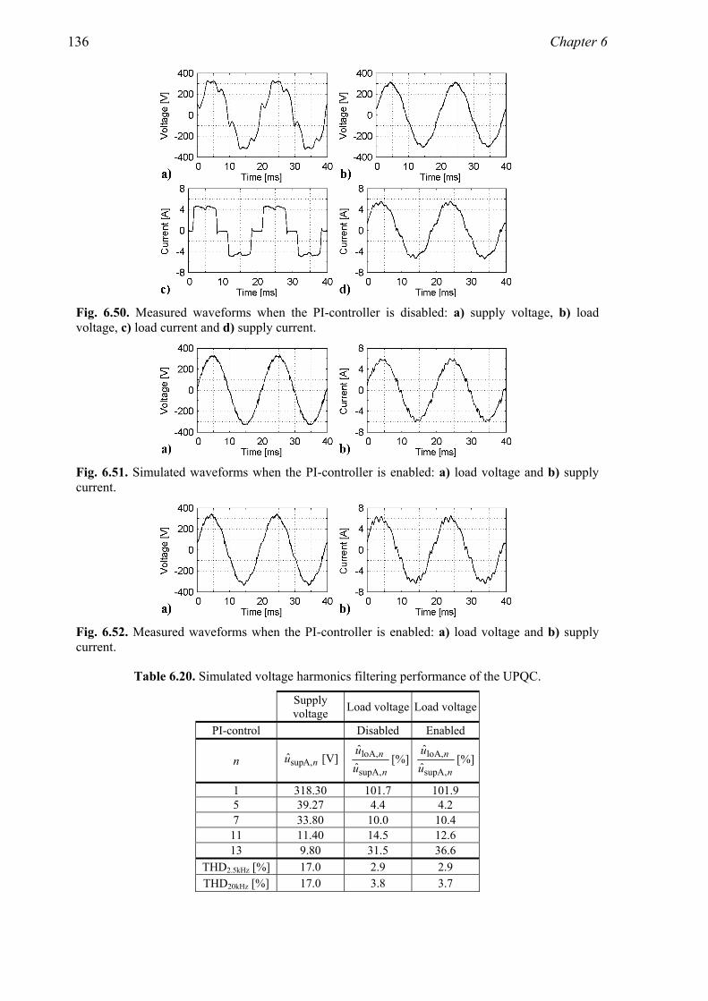
136 Chapter 6
Fig. 6.50. Measured waveforms when the PI-controller is disabled: a) supply voltage, b) load voltage, c) load current and d) supply current.
Fig. 6.51. Simulated waveforms when the PI-controller is enabled: a) load voltage and b) supply current.
Fig. 6.52. Measured waveforms when the PI-controller is enabled: a) load voltage and b) supply current.
Table 6.20. Simulated voltage harmonics filtering performance of the UPQC.
Supply voltage Load voltage Load voltage
PI-control Disabled Enabled
n nu A,supˆ [V] n
nuu
,supA
A,loˆˆ
[%] n
nuu
,supA
A,loˆˆ
[%]
1 318.30 101.7 101.95 39.27 4.4 4.2 7 33.80 10.0 10.4
11 11.40 14.5 12.6 13 9.80 31.5 36.6
THD2.5kHz [%] 17.0 2.9 2.9 THD20kHz [%] 17.0 3.8 3.7

Operation of the SHAPFs and the UPQC 137
Table 6.21. Simulated current harmonics filtering performance of the UPQC.
Load current Supply current
Supply current
PI-control Disabled Enabled
n ni A,loˆ [A] n
n
ii
A,lo
A,supˆˆ
[%]n
n
ii
A,lo
A,supˆˆ
[%]
1 4.95 115.8 116.05 1.12 4.4 5.2 7 0.60 10.8 11.9
11 0.47 19.5 19.9 13 0.27 58.6 62.1 17 0.27 82.0 72.3 19 0.17 71.0 64.6 23 0.15 59.2 56.7 25 0.11 41.6 39.3 29 0.09 47.9 45.8 31 0.08 33.4 45.7 35 0.05 38.2 43.3 37 0.05 47.0 35.1 41 0.03 18.8 43.3 43 0.03 33.0 12.6 47 0.03 63.5 41.5 49 0.02 28.7 46.0
THD2.5kHz [%] 29.0 6.1 5.9 THD20kHz [%] 29.0 6.3 6.1
Table 6.22. Measured voltage harmonics filtering performance of the UPQC.
Supply voltage Load voltage Load voltage
PI-control Disabled Enabled
n nu A,supˆ [V]n
nuu
,supA
A,loˆˆ
[%]n
nuu
,supA
A,loˆˆ
[%]
1 318.35 94.1 101.75 39.12 16.4 17.3 7 33.75 30.3 31.9
11 11.42 8.4 7.7 13 9.96 36.5 54.2
THD2.5kHz [%] 16.9 4.6 4.8 THD20kHz [%] 16.9 4.8 5.0

138 Chapter 6
Table 6.23. Measured current harmonics filtering performance of the UPQC.
Load current Supply current
Supply current
PI-control Disabled Enabled
n ni A,loˆ [A] n
n
ii
A,lo
A,supˆˆ
[%]n
n
ii
A,lo
A,supˆˆ
[%]
1 4.96 106.2 123.85 1.12 23.2 25.0 7 0.60 37.8 38.4
11 0.47 6.3 7.3 13 0.27 43.1 92.3 17 0.26 37.0 60.3 19 0.18 41.7 52.2 23 0.15 17.6 32.9 25 0.12 17.7 31.3 29 0.08 26.5 25.1 31 0.08 30.3 24.9 35 0.05 12.3 24.8 37 0.05 20.7 24.4 41 0.03 7.3 27.7 43 0.03 12.5 14.8 47 0.02 16.6 12.9 49 0.03 20.5 18.7
THD2.5kHz [%] 29.0 7.7 8.6 THD20kHz [%] 29.0 7.8 8.6
Based on the results it can be seen that the UPQC efficiently filters both current and voltage harmonics. In addition to this, there is no remarkable difference in the harmonic filtering performance in cases where the PI-control of the SAPF is disabled or enabled. Based on the results it can be stated that the simulation results agree well with the measurement results, although there are some differences similar to the previous results achieved using sinusoidal supply voltage. The supply voltage and the load current waveforms are again similar in the simulations and in the measurements because the measured waveforms were used as inputs of the simulation model. If the harmonic content of the voltage waveforms are compared to the limits of the standard EN 50160, which were presented in Tables 2.2 and 6.19, it can be seen that the UPQC improves the situation remarkably. Although the amplitudes of the 5th and 7th harmonic components of the supply voltage are twice as high as is specified in the standard, and the 11th and 13th harmonic components are as high as is specified in the standard, the harmonic content of the load voltage is well below the limits specified in the standard. This applies to both cases, where the PI-control is enabled and disabled. If then the harmonic contents of the currents are compared to the limits of the current harmonic standard IEC 61000-3-2, which were presented in Table 2.1, it can be seen that the harmonic contents of all currents are below the limits specified in the standard.
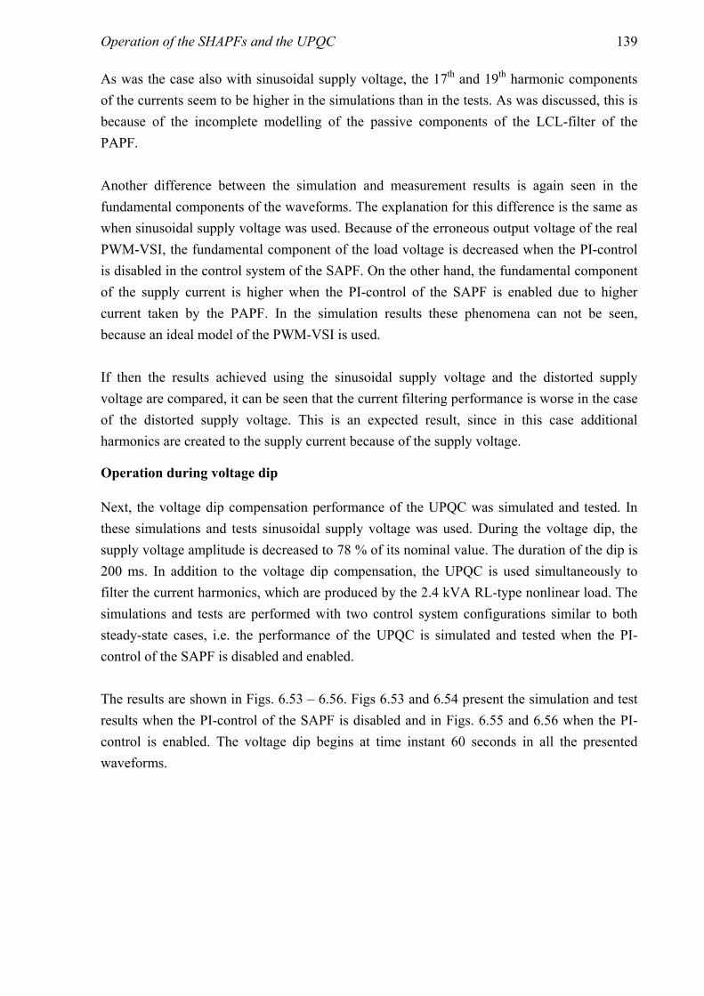
Operation of the SHAPFs and the UPQC 139
As was the case also with sinusoidal supply voltage, the 17th and 19th harmonic components of the currents seem to be higher in the simulations than in the tests. As was discussed, this is because of the incomplete modelling of the passive components of the LCL-filter of the PAPF. Another difference between the simulation and measurement results is again seen in the fundamental components of the waveforms. The explanation for this difference is the same as when sinusoidal supply voltage was used. Because of the erroneous output voltage of the real PWM-VSI, the fundamental component of the load voltage is decreased when the PI-control is disabled in the control system of the SAPF. On the other hand, the fundamental component of the supply current is higher when the PI-control of the SAPF is enabled due to higher current taken by the PAPF. In the simulation results these phenomena can not be seen, because an ideal model of the PWM-VSI is used. If then the results achieved using the sinusoidal supply voltage and the distorted supply voltage are compared, it can be seen that the current filtering performance is worse in the case of the distorted supply voltage. This is an expected result, since in this case additional harmonics are created to the supply current because of the supply voltage.
Operation during voltage dip
Next, the voltage dip compensation performance of the UPQC was simulated and tested. In these simulations and tests sinusoidal supply voltage was used. During the voltage dip, the supply voltage amplitude is decreased to 78 % of its nominal value. The duration of the dip is 200 ms. In addition to the voltage dip compensation, the UPQC is used simultaneously to filter the current harmonics, which are produced by the 2.4 kVA RL-type nonlinear load. The simulations and tests are performed with two control system configurations similar to both steady-state cases, i.e. the performance of the UPQC is simulated and tested when the PI-control of the SAPF is disabled and enabled. The results are shown in Figs. 6.53 – 6.56. Figs 6.53 and 6.54 present the simulation and test results when the PI-control of the SAPF is disabled and in Figs. 6.55 and 6.56 when the PI-control is enabled. The voltage dip begins at time instant 60 seconds in all the presented waveforms.
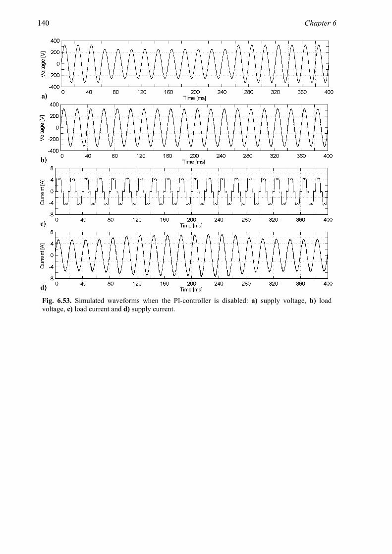
140 Chapter 6
Fig. 6.53. Simulated waveforms when the PI-controller is disabled: a) supply voltage, b) load voltage, c) load current and d) supply current.

Operation of the SHAPFs and the UPQC 141
Fig. 6.54. Measured waveforms when the PI-controller is disabled: a) supply voltage, b) load voltage, c) load current and d) supply current.

142 Chapter 6
Fig. 6.55. Simulated waveforms when the PI-controller is enabled: a) supply voltage, b) load voltage, c) load current and d) supply current.

Operation of the SHAPFs and the UPQC 143
Fig. 6.56. Measured waveforms when the PI-controller is enabled: a) supply voltage, b) load voltage, c) load current and d) supply current.
Based on the presented supply current waveforms, it can be seen that the supply current harmonics can be filtered simultaneously with the voltage dip compensation using the UPQC. In the figures it can also be seen that the fundamental component of the current is increased during the voltage dip. The current increases because the PAPF draws more current at the fundamental frequency during the dip, as has been earlier explained. Based on the results, the voltage dip occurring in the supply voltage can be compensated efficiently using the UPQC. Based on the load voltage waveforms, differences can be seen in the performance of the UPQC between cases where the PI-control of the SAPF is disabled and enabled. When the PI-control is disabled, the amplitude of the load voltage seems to be lower before, during and after the voltage dip compared with when the PI-control is enabled. This is because the amplitude of the fundamental component of the load voltage is closer to its reference value when the PI-control is enabled. This was shown already earlier in the case of the steady-state simulations and tests.

144 Chapter 6
In addition to this, in the measured waveform presented in Fig. 6.56b it can be seen that the amplitude of the load voltage decreases for a half of the fundamental cycle in the beginning and immediately after the voltage dip when PI-control is used. This is because of the functioning of the control system of the SAPF, which was presented in Section 3.7.1. Whenever the control system observes a dynamic change in the supply voltage, the PI-control of the SAPF is disabled in order to guarantee a fast response of the SAPF. The PI-control is again enabled automatically after the supply voltage change. Since it is hard to see the variations of the supply and load voltages presented in Figs. 6.53 – 6.56, the RMS values of these voltages are presented in Figs. 6.57 and 6.58.
Fig. 6.57. Calculated RMS values of the simulated voltages: supply voltage (Δ), load voltage (PI-controller disabled, x) and load voltage (PI-controller enabled, o).
Fig. 6.58. Calculated RMS values of the measured voltages: supply voltage (Δ), load voltage (PI-controller disabled, x), load voltage (PI-controller enabled, o).
The RMS voltages were calculated using
( ) ∑+−=
=k
Nkiiu
NkU
1
2RMS
1 , (6.1)
where k is the ordinal number of the datapoint and N = 2000, which corresponds to one fundamental period, i.e. 20 ms (Bollen, 1999). Since the calculated RMS value corresponds to 20 ms of the voltage data prior to a given time instant, the calculation of the instantaneous RMS values was begun 20 ms before the beginning of the waveforms shown in Figs. 6.53 – 6.56.

Operation of the SHAPFs and the UPQC 145
First it has to be noticed that based on Figs. 6.57 and 6.58, conclusions can be drawn only in the steady-state operation. Since each of the RMS values presents the instantaneous voltage values during the past 2000 samples, the calculation of these RMS values makes sense only if the voltage does not fluctuate during these 2000 samples. This can be seen in the beginning and in the end of the supply voltage dip, where the RMS value of the supply voltage changes slowly, although in reality the voltage is changed stepwise, as could be seen in Figs. 6.53a, 6.54a, 6.55a and 6.56a. In the simulation results presented in Fig. 6.57 nothing special is seen. This is because of the ideal simulation model of the PWM-VSI. However, Fig. 6.58 shows, interestingly, how the control system of the SAPF operates. When the PI-control of the SAPF is disabled, it can be seen that the load voltage is continuously about 20 Volts below the nominal value 230 Volts. Since the supply voltage is 78 % of the nominal value during the dip, the situation is improved thanks to UPQC, since the load voltage is 91 % of the nominal value. However, it can be seen that before and after the supply voltage dip the load voltage is also 91 % of the nominal value, which is a problem since the supply voltage is at its nominal value 230 V. The main reason for this is the erroneous output voltage of the PWM-VSI, which is caused by its non-idealities and which can not be corrected using an open loop control. This was clarified when the steady-state results of the UPQC were discussed. However, in the case where the PI-control of the SAPF is enabled, it can be seen that the load voltage is at its reference value before and after the supply voltage dip, i.e. the steady-state error of the load voltage can be decreased to zero using the PI-control. In the beginning and after the supply voltage dip the load voltage fluctuates since the PI-control is disabled because of the dynamic change in the supply voltage. When the steady-state operation is again reached, the PI-control is automatically enabled and the error between the load voltage and its reference value 230 Volts decreases to zero.
Operation during stepwise changing load current
Lastly, the operation of the UPQC during the stepwise changing load current was simulated and tested. Sinusoidal supply voltage is used in these simulations and tests. In these simulations and tests the 2.4 kVA RL-type nonlinear load is used. The change in the load current is achieved by changing the value of the load resistor between the values 104 Ω (2.4 kVA) and 206 Ω (1.2 kVA). In these simulations and tests the PI-control of the SAPF was enabled. The results of the simulations and tests are shown in Figs. 6.59 – 6.62. Figs 6.59 and 6.60 present the simulated and measured waveforms in the case of decreasing load current and in Figs. 6.61 and 6.62 in the case of increasing load current.

146 Chapter 6
Fig. 6.59. Simulated waveforms: a) load current and b) supply current.
Fig. 6.60. Measured waveforms: a) load current and b) supply current.
Fig. 6.61. Simulated waveforms: a) load current and b) supply current.
Fig. 6.62. Measured waveforms: a) load current and b) supply current.
Based on the results it can be stated that the current filtering performance of the UPQC is not decreased during the stepwise current change. The supply current remains almost sinusoidal during the change and its amplitude reaches its new value smoothly in about three fundamental cycles.
6.3 Summary
This chapter presented the results of the simulations and prototype tests of three SHAPFs and the UPQC. The beginning of the chapter presentsed the SHAPF results. The current filtering performance of the SCT, FCT and the ETLC in steady-state operation was simulated and tested using RL and RC-type nonlinear loads with several different configurations. The aim was to minimise the harmonic content of the supply current using the given parameters.

Operation of the SHAPFs and the UPQC 147
First of all the current harmonics filtering performances of the passive filters of the SHAPF topologies were examined, i.e. the APF was not yet connected to the main circuit. As a result, it was stated that when using the passive filters of the SCT/FCT the amplitudes of the current harmonics are still too high if they are compared to International Standard IEC 61000-3-2. The supply current THD could be decreased to 15 % in the case of RL-type nonlinear load and to 24 % in the case of RC-type nonlinear load, whereas the respective load current THDs were 26 % and 41 %. The current harmonics filtering performance of the passive filter of the ETLC was distorted by the resonance at the 5th harmonic frequency. In the following cases the APF was connected to the main circuit and the simulations and tests were performed in cases where the LC-filter was, and was not, used in the output of the PWM-VSI. Based on the results the current filtering performance of all topologies was slightly worse in the first case. The current filtering performance of the SCT was found to be the best. In the measurements where the LC-filter was not used, the supply current THD 4 % was reached with both RL and RC-type nonlinear loads. The filtering performance of the FCT was the second best, THD values 7 % and 17 % could be reached in the respective test cases. The filtering performance of the ETLC was the worst, the respective measured supply current THDs were 16 % and 27 %. However, the filtering performance of the ETLC could be enhanced using the control system, which is capable of generating active resistance in addition to active inductances. It was also noticed that the resonance of the passive filter of the ETLC, which occurred at the 5th harmonic frequency, was removed thanks to APF operation. Also the efficiencies of the topologies were calculated based on the measurement results. The efficiencies of the SHAPFs were found to be very close to each other and close to 95 % with both loads. The current harmonics filtering performance of the SCT and the FCT was also examined in the case where the dc-link voltage was maintained using the three-phase diode rectifier instead of dc-link voltage control. In this case it was seen that the current filtering performance of the SHAPFs is enhanced if the dc-link voltage is maintained using an auxiliary power supply. In the case of RL-type nonlinear load the supply current THD was decreased by 0.3 percentage units with the SCT and 1.3 percentage units with the FCT based on the measurements. Respectively, in the case of the RC-type nonlinear load the THD was decreased by 0.3 percentage units with the SCT and 5.5 percentage units with the FCT. In addition to this, it was observed that increasing the dc-link voltage enhanced the current filtering performance of both SHAPFs since in this case higher active resistance could be used. The behaviour of the SHAPFs was also researched in the case of stepwise changing load current. Based on the results it was seen that all topologies also operate with this kind of load.

148 Chapter 6
After this the operation of the UPQC was simulated and tested. In all simulations and tests the RL-type nonlinear load was used. The steady-state filtering performance was simulated and tested with two control system configurations. In the first case the PI-control of the SAPF was disabled and in the second case enabled. First, the supply current filtering performance of the UPQC was researched using sinusoidal supply voltage. In the second case distorted supply voltage was used in order to inspect the supply voltage harmonics filtering performance simultaneously. Based on the results it could be seen that the UPQC filters both current and voltage harmonics efficiently. Based on the measurements, in the case of the sinusoidal supply voltage the supply current THD could be decreased to 6 % when the load current THD was 28 %. In the other case distorted supply voltage, the THD of which was 17 %, was used. In this case the supply current THD could be decreased to 8 %, while the load voltage THD was decreased to 5 %. It was noticed that the PI-control of the SAPF had no significant influence on the harmonics filtering performance. However, using the PI-control in the control system of the SAPF, the steady-state error occurring in the fundamental component of the load voltage could be decreased to zero. The efficiency of the UPQC was found to be about 95 %. The behaviour of the UPQC in dynamic changes was tested in two cases. In the first one the voltage dip compensation performance of the UPQC was simulated and tested. In this case it was shown that the UPQC compensates the voltage dip occurring in the supply voltage efficiently simultaneously with supply current harmonics filtering. During the voltage dip, the supply voltage was 78 % of its nominal value 230 V. When the PI-control of the SAPF was not used, the load voltage could be corrected to 91 % of the reference value. By using the PI-control of the SAPF the steady-state error of the load voltage could be completely removed. Lastly, the operation of the UPQC was simulated and tested during stepwise changing load current. Based on the results it was seen that the filtering performance of the UPQC is also good in this case.

Conclusions 149
7 Conclusions
The main objective of this thesis was to research the power conditioning capabilities of the series active power filter (SAPF) and hybrid active power filters (HAPFs) based on it. The research of the power conditioning capabilities was done by inspecting the current and voltage harmonics filtering and voltage dip compensation performance of these filters. The research on the current harmonics filtering performance was done by inspecting the operation and characteristics of three series hybrid active power filter (SHAPF) topologies and by comparing their current harmonics filtering performance. This was one of the scientific contributions of this thesis. These SHAPFs were called supply connected topology (SCT), filter connected topology (FCT) and electrically tuned LC shunt circuit (ETLC). The basic operating principles of these SHAPFs were discussed in Chapter 3. The operation and characteristics of the SHAPFs were researched using computer simulations and experimental tests. The modelling and structures of the simulation models of the SHAPFs were presented in Chapter 4. Chapter 5 presented the prototype of the pulse width modulated voltage source inverter (PWM-VSI), which was used as a part of the SHAPF prototypes used for testing. The results of the simulations and experimental tests were presented in Chapter 6. The current harmonics filtering performance of the SCT, FCT and ETLC was simulated and tested in stationary operation using different nonlinear loads and main circuit and control system configurations. The aim in the steady-state tests was to minimise the harmonic content of the supply current. According to the results, the current harmonics filtering performance of the SCT was the best. The filtering performance of the FCT was nearly the same as with the SCT and the filtering performance of the ETLC was the worst. However, the filtering performance of the ETLC could be enhanced using the control system, which is capable of generating active resistance in addition to the active inductances. This validated one of the scientific contributions of this work, which was to improve the original control system of the ETLC such that it is capable of applying also active resistance. Based on the simulations and tests performed with the SCT and FCT, where the dc-link voltage was maintained using a three-phase diode rectifier instead of the dc-link voltage control, it was stated that the current filtering performance of the SHAPFs is enhanced if the dc-link voltage is maintained using an auxiliary power supply. In addition to this it was shown that increasing of dc-link voltage enhances the current filtering performance of the SHAPFs since in this case higher active resistance can be used. The current filtering performance of the SHAPFs was also examined in the case of stepwise

150 Chapter 7
changing load current. Based on the results it was seen that all topologies are capable of current filtering also during the load current change. One of the author’s contributions was to propose the improvement of the control systems of the SHAPFs, which prevents the saturation of the coupling transformer. Based on the measurements carried out with SHAPF prototypes the improvement was found to be effective and the saturation did not occur. The voltage harmonics filtering performance and the voltage dip compensation performance were researched by inspecting the functioning of the unified power quality conditioner (UPQC), which consists of the parallel active power filter (PAPF) and the SAPF. The objective, and one of the scientific contributions of this thesis, was to research the operation and characteristics of the UPQC and to develop the control system of the SAPF in order to improve its voltage dip compensation performance. The procedure of the research work was similar as with the SHAPFs, i.e. the operation and characteristics of the UPQC were inspected using mathematical models, computer simulations and experimental tests. The operating principle of the UPQC was first introduced in Chapter 3. The modelling and the simulation models of the UPQC were presented in Chapter 4. The prototype of the PWM-VSI, which was presented in Chapter 5, was used to constitute the prototype of the UPQC used for testing. The simulation and experimental test results were presented in Chapter 6. The operation of the UPQC was simulated and tested in stationary operation and in dynamic changes using a nonlinear load. The steady-state current and voltage filtering performance was simulated and tested using sinusoidal and distorted supply voltage. The steady-state simulations and tests were performed with two control system configurations. In the first one, only P-controller was used with the SAPF and in the other one the proposed PI-control method was used in addition to this. It was seen that the proposed PI-control method had no significant influence on the current or voltage harmonics filtering performance. However, when using the proposed PI-control method, the steady-state error occurring in the fundamental component of the load voltage could be decreased to zero. The behaviour of the UPQC in dynamic changes was tested in two cases. In the first one, the voltage dip compensation performance of the UPQC was tested. In the other, the operation of the UPQC during the stepwise changing load current was examined. In the voltage dip compensation test it was seen that the UPQC compensates the voltage dip occurring in the supply voltage efficiently and the proposed PI-control method also works in this case by decreasing the steady-state error of the load voltage at the fundamental frequency immediately after the supply voltage change. This validated the functioning of the improved control system of the UPQC, which was proposed by the author. In the test, where the load current was changed stepwise it was seen that the UPQC filters current harmonics efficiently

Conclusions 151
also in this case. In general, the achieved results can be held to be valid and the original objectives set were achieved. The simulation models, which were realised based on the mathematical models of the systems, were found to be sufficiently precise at the inspected frequency range. This could be verified by comparing the simulation and test results. In addition to this, since the same conclusions could be made based on both simulation and measurement results, these conclusions can be regarded as reliable. A minor drawback of this research work is that the achieved results are topology-specific and cannot be generalised to other active power filters (APFs). Instead, although the low power prototypes were inspected in this work, the conclusions concerning the presented topologies can be regarded also to hold true to some extent at higher power levels. However, it has to be noticed that at higher power levels it may be preferable to use other design parameters in the SHAPF design than would be achieved by scaling the parameters used in this work to the inspected power level. Examples of these parameters are the parameters of the LC shunt circuits and coupling transformer. This different parameter optimisation may have influence on some of the conclusions. In this thesis it was shown that the SAPF can be used efficiently to filter current and voltage harmonics and to compensate voltage dips. Although the subject of this thesis was restricted to these phenomena, it would also be interesting to research the compensation capabilities of the SAPF in the case of other disturbances existing in the electric network. One very interesting task would be to research the current or voltage harmonics filtering performance or the voltage dip compensation performance of the SAPF in the case of unsymmetrical disturbances, since only symmetrical three-phase distortions were inspected in this work. This inspection could include the research of four-wire SAPF, which is also capable of filtering zero sequence distortions. This kind of device has rarely been an object of research work. This topology is realised using the wye-connected coupling transformer and the PWM-VSI, whose dc-link is constructed of two series connected capacitors. In this topology the mid-point of the dc-link capacitors, wye point of the coupling transformer and wye point of the LC-filter capacitors are connected together. Another interesting task would be the comparison of the SHAPFs and PAPF. This research work could include the inspection of the current harmonics filtering performance, losses and costs of the chosen topologies. The last item on the list, the costs of the topology, would be an especially interesting subject of research since it could be investigated whether any SHAPF topology with the same current harmonics filtering performance can compete with the PAPF from the economic point of view.

152 Chapter 7
In conclusion, based on the results presented in this thesis it can be stated that the SAPF is a versatile and efficient tool for power conditioning. The drawbacks of the pure SAPF can be overcome by using HAPFs that are based on the SAPF instead of the pure SAPF. Although the inspected electric systems were low power ones, the most attractive application area of the SAPF is in medium power applications. This is because the SAPF is connected in series with the system using the coupling transformer, which can be used to match the power levels of the electric system and the inverter included in the SAPF. Therefore, as power quality becomes more and more important matter in the future, the SAPF is likely to be the potential tool for power conditioning especially in medium power applications.

153
References
ABB (2004), PowerIT Liquid Filled Transformers – IEC Standard, Small and Medium, Rated Power ≤ 2000 kVA, HV ≤ 36 kV, brochure, ABB Transformers Power Technologies Division, 2004.
ABB (2007), PowerITPienjänniteverkon aktiivisuodattimet – PQFI – PQFM – PQFK – PQFS, brochure, ABB Oy, 2007. (in Finnish)
Acha, E., Agelidis, V., Anaya-Lara, O., Miller, T. (2002), Power Electronic Control in Electrical Systems, Newnes Publishers, 443 p., 2002.
Akagi, H., Kanazawa, Y., Nabae, A. (1984), Instantaneous Reactive Power Compensators Comprising Switching Devices without Energy Storage Components, IEEE Transactions on Industry Applications, Vol. IA-20, No. 3, pp. 625 – 630, May 1984.
Akagi, H. (1996), New Trends in Active Filters for Power Conditioning, IEEE Transactions on Industry Applications, Vol. 32, No. 6, pp. 1312-1322, November 1996.
Akagi, H. (2000), Active and Hybrid Filters for Power Conditioning, Proceedings of the IEEE International Symposium of Industrial Electronics, Vol. 1, pp. TU26-TU36, December 2000.
Akagi, H., Watanabe, E., Aredes, M. (2007), Instantaneous Power Theory and Applications to Power Conditioning, John Wiley & Sons, Inc. - IEEE Press, New Jersey, USA, 379 p., 2007.
Arcotronics (2008), MKP Series Capacitor Specifications, datasheet, Arcotronics group.
Arrillaga, J., Watson, N. (2003), Power System Harmonics, 2nd edition, John Wiley & Sons, Inc., Chichester, England, 399 p., 2003.
Bhattacharya, S., Divan, D. (1995), Synchronous Frame Based Controller Implementation for a Hybrid Series Active Filter System, Conference Record of the IEEE Industry Applications Conference, Vol. 3, pp. 2531-2540, October 1995.
Bhattacharya, S., Cheng, P., Divan, D. (1997), Hybrid Solutions for Improving Passive Filter Performance in High Power Applications, IEEE Transactions on Industry Applications, Vol. 33, No. 3, pp. 732-747, May 1997.
Bollen, M. (1999), Understanding Power Quality Problems: Voltage Sags and Interruptions, John Wiley & Sons, Inc. - IEEE Press, New York, USA, 543 p., 1999.
154 References
Cheng, P., Huang, C., Pan, C., Bhattacharya, S. (2003), Design and Implementation of a Series Voltage Sag Compensator Under Practical Utility Conditions, IEEE Transactions on Industry Applications, Vol. 39, No. 3, pp.844 - 853, May 2003.
Dai, K., Liu, P., Xiong, J., Chen, J. (2003), Study on Dual-DSP-Controlled Three-Phase Series-Parallel Compensated Line-Interactive UPS System (Delta-Conversion UPS), Proceedings of the IEEE International Electric Machines and Drives Conference, Vol. 1, pp. 436 – 443, June 2003.
Das, J. (2004), Passive Filters – Potentialities and Limitations, IEEE Transactions on Industry Applications, Vol. 40, No. 1, pp. 232-241, January 2004.
da Silva, S., Donoso-Garcia, P., Cortizo, P., Seixas, P. (2002), A Three-Phase Line-Interactive UPS System Implementation With Series-Parallel Active Power-Line Conditioning Capabilities, IEEE Transactions on Industry Applications, Vol. 38, No. 6, pp. 1581 – 1590, November 2002.
de Leon, F., Samlyen, A. (1993), Time Domain Modeling of Eddy Current Effects for Transformer Transients, IEEE Transactions of Power Delivery, Vol. 8, No. 1, pp. 271 – 280, January 1993.
de León, F., Samlyen, A. (1995), A Simple Representation of Dynamic Hysteresis Losses in Power Transformers, IEEE Transactions on Power Delivery, Vol. 10, No. 1, pp. 315 – 321, January 1995.
Divan, D. (1984), Non Dissipative Switched Networks for High Power Applications, Electronics Letters, Vol. 20, No. 7, pp. 277 – 279, March 1984.
Djokić, S., Stockman, K., Milanović, J., Desmet, J., Belmans, R. (2005), Sensitivity of AC Adjustable Speed Drives to Voltage Sags and Short Interruptions, IEEE Transactions on Power Delivery, Vol. 20, No. 1, pp. 494 – 505, January 2005.
Doležal, J., Castillo, A., Tlustý, J., Valouch, V. (2000), Topologies and Control of Active Filters for Flicker Compensation, Proceedings of the International Symposium on Industrial Electronics, Vol. 1, pp. 90-95, December 2000.
Domijan, A., Embriz-Santander, E. (1992), A Summary and Evaluation of Recent Developments on Harmonic Mitigation Techniques Useful to Adjustable Speed Drives, IEEE Transactions on Energy Conversion, Vol. 7, Issue 1, pp. 64-71, March 1992.
Dorf, R., Bishop, R. (1998), Modern Control Systems, Addison Wesley Longman, California, USA, 855 p., 1998.
EIA (2000), The Changing Structure of the Electric Power Industry 2000: An Update, Energy Information Administration, Report No. DOE/EIA-0562(00), Washington DC, USA, October 2000.
155
EIA (2008), Annual Energy Outlook 2008 – With Projections for 2030, Energy Information Administration, Report No. DOE/EIA-0383(2008), Washington DC, USA, March 2008.
El-Habrouk, M., Darwish, M., Mehta, P. (2000), Active Power Filters: A Review, IEEE Proceedings on Electric Power Applications, Vol. 147, No. 3, pp. 844-853, September 2000.
El-Saadany, E. (2001), Effectiveness of Different Filtering Methodologies in Harmonic Distortion Mitigation, Proceedings of Canadian Conference on Electric and Computer Engineering, Vol. 2, pp. 1035-1040, May 2001.
Emadi, A., Nasiri, A., Bekiarov, S. (2005), Uninterruptible Power Supplies and Active Filters, CRC Press, Florida, USA, 276 p., 2005.
Evox Rifa (2008), PEH200 Electrolytic Capacitor Specifications, datasheet, Evox Rifa group.
Finland Ministry of Trade and Industry (1997), Energiatalous 2025 – Skenaariotarkasteluja, Finland Ministry of Trade and Industry (Kauppa- ja teollisuusministeriö), Publications 3/1997, 95 p., February 1997. (in Finnish)
Finnish Electricity Market Act (1995), Finnish Electricity Market Act (Sähkömarkkinalaki) 368/1995, March 1995. (in Finnish)
Freescale (2003), MPC-561/MPC563 Reference Manual, Freescale Semiconductor, Inc., 2003.
Fujita, H., Akagi, H. (1991), A Practical Approach To Harmonic Compensation in Power Systems – a Series Connection of Passive and Active Filters, IEEE Transactions on Industry Applications, Vol. 27, pp. 1020-1025., November 1991.
Fujita, H., Akagi, H. (1996), The Unified Power Quality Conditioner: The Integration of Series Active Filters and Shunt Active filters, IEEE Transactions on Power Electronics, Vol. 13, pp. 315-322, March 1996.
Funato, H., Kawamura, A. (1992), Proposal of Variable Active-Passive Reactance, Proceedings of the Annual Conference of the IEEE Industrial Electronics Society, Vol. 1, pp. 381 – 388, 1992.
Funato, H., Kawamura, A. (1993), Analysis of Variable Active-Passive Reactance, Proceedings of the Power Conversion Conference, pp. 647 – 652, 1993.
Grady, W., Samotyj, M., Noyola, A. (1990), Survey of Active Power Line Conditioning Methodologies, IEEE Transactions on Power Delivery, Vol. 5, No 3, pp. 1536-1542, July 1990.
Green, T., Marks, J. (2005), Control Techniques for Active Power Filters, IEE Proceedings of Electric Power Applications, Vol. 152, Issue 2, pp. 369-381, March 2005.

156 References
Guru, B., Hiziroğlu, H. (2001), Electric Machinery and Transformers, 3rd edition, Oxford University Press, New York, USA, 700 p., 2001.
Gyugyi, L., Strycula, E. (1976), Active AC Power Filters, Proceedings of IEEE IAS Annual Meeting, pp. 529-525. 1976.
Gyugui, L., Schauder, C., Williams, S., Rietman, T., Torgerson, D., Edris, A. (1995), The Unified Power Flow Controller: A New Approach to Power Transmission Control, IEEE Transactions on Power Delivery, Vol. 10, No. 2, pp. 1085 – 1097, April 1995.
Heydt, G. (1998), Electric Power Quality: A Tutorial Introduction, IEEE Computer Applications in Power, Vol. 11, Issue 1, pp. 15-19, January 1998.
Holmes, D., Lipo, T. (2003), Pulse Width Modulation for Power Converters – Principles and Practice, John Wiley & sons, Inc. - IEEE Press, New Jersey, USA, 724 p., 2003.
ITIC (2000), ITI (CBEMA) curve, Information Technology Industry Council, Washington DC, USA, http://www.itic.org/archives/iticurv.pdf, January 2000.
Jenkins, N., Allan, R., Crossley, P., Kirschen, D., Strbac, G. (2000), Embedded Generation, The Institution of Electrical Engineers, London, UK, 273 p., 2000.
Johnson, J. (2002), Proper Use of Active Harmonic Filters to Benefit Pulp and Paper Mills, IEEE Transactions on Industry Applications, Vol. 38, No. 3, pp. 719-725, May 2002.
Karthik, K., Quaicoe, J. (2000), Voltage Compensation and Harmonic Suppression Using Series Active and Shunt Passive Filters, Proceedings of Canadian Conference on Electrical and Computer Engineering, Vol. 1, pp. 582-586, March 2000.
Kazmierkowski, M., Krishnan, R., Blaabjerg, F. (2002), Control in Power Electronics – Selected Problems, Academic Press, San Diego, USA, pp. 89 – 160, 2002.
Kawahira, H., Nakamura, T., Nakazawa, S., Nomura, M. (1983), Active Power Filters, Proceedings of the International Power Electronics Conference, pp. 981 – 992, March 1983.
Kovács, K., Rácz, I. (1959), Transiente Vorgänge in Wechselstrommaschinen, Verlag der Ungarischen Akademie der Wissenschaften, Budabest, Hungary, 267 p., 1959. (In German)
Lai, J., Key, T. (1997), Effectiveness of Harmonic Mitigation Equipment for Commercial Office Buildings, IEEE Transactions on Industry Applications, Vol. 33, No. 4, pp. 1104-1110, July 1997.
Lamoree, J., Mueller, D., Vinett, P., Jones, W., Samotyj, M. (1994), Voltage Sag Analysis Case Studies, IEEE Transactions on Industry Applications, Vol. 30, No. 4, pp. 1083 – 1089, July 1994.

157
Levonen, M. (2006), Microcontroller Based Control of Four-Wire Current Source Rectifier, Master of Science Thesis, Tampere, TUT, Degree program in Electrical Engineering, 79 p., June 2006. (in Finnish)
Mannila, T., Hovila, J., Trygg, P., Laitinen, K., Kuusiluoma, S., Korpinen, L. (2000), The Electricity Production and Market Liberalization in the European Union, Proceedings of International Conference on Power System Technology, Vol. 3, pp. 1641-1645, December 2000.
Mariethoz, S., Rufer, A. (2002), Open Loop and Closed Loop Spectral Frequency Active Filtering, IEEE Transactions on Power Electronics, Vol. 17, No. 4, July 2002.
Martinez, J., Mork, B. (2005), Transformer Modeling for Low- and Mid-Frequency Transients – a Review, IEEE Transactions on Power Delivery, Vol. 20, No. 2, April 2005.
Massoud, A., Finney, S., Williams, B. (2004), Seven-Level Shunt Active Power Filter, Proceedings of IEEE International Conference on Harmonics and Quality of Power, 6 p., September 2004.
Matsch, L., Morgan, J. (1987), Electromagnetic and Electromechanical Machines, 3rd edition, John Wiley & Sons, Inc., 574 p.
McGranaghan, M., Kennedy, B., Samotyj, M. (1998), Power Quality Contracts in a Competitive Electric Utility Industry, Proceedings of 8th International Conference on Harmonics and Quality of Power, Vol. 1, pp. 170-175, October 1998.
McPherson, G., Laramore, R. (1990), An Introduction to Electrical Machines and Transformers, 2nd edition, John Wiley & Sons, Inc., 571 p.
Mohan, N., Peterson, H., Long, W., Dreifuerst, G., Vithayathil, J. (1977), Active Filters for AC Harmonic Suppression, Proceedings of the IEEE-PES Winter Meeting, paper A77026-8, January 1977.
Mohan, N., Undeland, T., Robbins, W. (1995), Power Electronics – Converters, Applications and Design, 2nd edition, John Wiley & Sons, Inc., 802 p., 1995.
Morán, L., Dixon, J., Espinoza, J., Wallace, R. (1999), Using Active Power Filters to Improve Power Quality, Proceedings of 5th Brazilian Power Electronics Conference, September 1999.
Nam, K., Choi, S., Ryoo, H., Jeong, S., Lee, J., Kim, D. (2004), Development of Criteria and Calculation of Korean Industrial Customer Interruption Costs, Proceedings of International Conference on Power Systems Technology, pp. 592-597, November 2004.
Niiranen, J. (1997), Tehoelektroniikan komponentit, Otatieto Oy, Helsinki, Finland, 233 p. (in Finnish)
158 References
Nokian Capacitors (2006), MaxSine active filter, brochure, Nokian Capacitors Ltd., 2006.
Novotny, D., Lipo, T. (1996), Vector Control and Dynamics of AC Drives, Oxford University Press, Oxford, UK. 440 p., 1996.
Ollila, J., (1993), Analysis of PWM-Converters Using Space Vector Theory – Application to a Voltage Source Rectifier, Doctoral thesis, Tampere University of Technology Publications 111, 167 p., 1993.
Peng, F., Akagi, H., Nabae, A. (1990), A New Approach to Harmonic Compensation in Power Systems – A Combined System of Shunt Passive and Series Active Filters, IEEE Transactions on Industry Applications, Vol. 26, No. 6, pp. 983-990, November 1990.
Peng, F., Akagi, H., Nabae, A. (1993), Compensation Characteristics of the Combined System of Shunt Passive and Series Active Filters, IEEE Transactions on Industry Applications, Vol. 29, No. 1, pp. 144-152, January 1993.
Peng, F. (1998), Application Issues of Active Power Filters, IEEE Industry Applications Magazine, Vol. 4, pp. 21-30, September 1998.
Peng, F. (2001), Harmonic Sources and Filtering Approaches, IEEE Industry Applications Magazine, Vol. 7, pp. 18-25, July 2001.
Pettersson, S. (2004), Implementation and Microcontroller Based Control of a Four-Wire Active Power Filter, Master of Science Thesis, Tampere, TUT, Degree program in Electrical Engineering, 102 p., March 2004. (in Finnish)
Rivas, D., Morán, L., Dixon, J., Espinoza, J. (2002), A Simple Control Scheme for Hybrid Active Power Filter, IEE Proceedings of Generation, Transmission and Distribution, Vol. 149, No. 4, July 2002.
Rivas, D., Morán, L., Dixon, J., Espinoza, J. (2003), Improving Passive Filter Compensation Performance with Active Techniques, IEEE Transactions on Industrial Electronics, Vol. 50, No. 1, pp. 161-170, February 2003.
Routimo, M. (2002), Microcontroller Based Control of a Voltage Source Active Power Filter, Master of Science Thesis, Tampere, TUT, Degree program in Electrical Engineering, 89 p., February 2002. (in Finnish)
Routimo, M., Salo, M., Tuusa, H. (2003), A Control Delay Compensation Method for Voltage Source Active Power Filter, Proceedings of the 9th European Power Quality Conference, pp. 93-97, May 2003.
Salo, M. (2002), Microcontroller Based Control of Current-Source PWM Converter Applications, Doctoral thesis, Tampere University of Technology Publications 399, 150 p., 2002.

159
Sasaki, H., Machida, T. (1971), A New Method to Eliminate AC Harmonic Currents by Magnetic Flux Compensation – Considerations on Basic Design, IEEE Transactions on Power Apparatus and Systems, Vol. 90, No. 5, September 1971.
Sasaki, H., Machida, T. (1974), Transient Analysis of Harmonic Current Elimination Method by Magnetic Flux Compensation, IEEE Transactions on Power Apparatus and Systems, Vol. 93, No. 2, March 1974.
Sueker, K., Hummel, S., Argent, R. (1989), Power Factor Correction and Harmonic Mitigation in a Thyristor Controlled Glass Melter, IEEE Transactions on Industry Applications, Vol. 25, No. 6, pp. 972-975, November 1989.
Sullivan, M., Vardell, T., Johnson, M. (1997), Power Interruption Costs to Industrial and Commercial Customers of Electricity, IEEE Transactions on Industry Applications, Vol. 33, No. 6, pp. 1448-1458, November 1997.
Takeda, M., Ikeda, K., Tominaga, Y. (1987), Harmonic Current Compensation with Active Filter, Proceedings of IEEE IAS Annual Meeting, pp. 808 – 815, 1987.
Turunen, J. (2003), Simulation and Implementation of Hybrid Filter, Master of Science Thesis, Tampere, TUT, Degree program in Electrical Engineering, 96 p., January 2003. (in Finnish)
Turunen J., Tuusa, H. (2006), Improvement of the Compensation Performance of UPQC, Proceedings of the Nordic Workshop on Power and Industrial electronics, 7p., June 2006.
Turunen J., Tuusa, H. (2007), Improvement of the Voltage Compensation Performance of the Series Active Power Filter Using a Simple PI-Control Method, Proceedings of 12th European Conference on Power Electronics and Applications, 9p., September 2007.
Turunen, J., Tuusa, H. (2008), Design Aspects of the Series Active Power Filter, International Review of Electrical Engineering, Vol. 3, No. 1, pp. 72-82., February 2008.
Van den Bossche, A., Valchev, V. (2005), Inductors and Transformers for Power Electronics, CRC Press, Florida, USA, 447 p., 2005.
Vas, P. (1992), Electrical Machines and Drives: a Space Vector Theory Approach, Clarendon Press, Oxford, UK, 808 p., 1992.
Wang, Z., Wang, Q., Yao, W., Liu, J. (2001). A Series Active Power Filter Adopting Hybrid Control Approach. IEEE Transactions on Power Electronics, Vol. 16, No. 3, pp. 301-310, May 2001.
Zobaa, A. (2004), Harmonics Problems Produced from the Use of Adjustable Speed Drives in Industrial Plants: Case Study, Proceedings of 11th International Conference on Harmonics and Quality of Power, pp. 6-10, September 2004.

160 References
Standards
ANSI C82.77-2002 American National Standard, Harmonic Emission Limits – Related to Power Quality Requirements for Lighting Equipment, January 2002.
EN 50160 European Standard, Voltage Characteristics of Electricity Supplied by Public Distribution Systems, November 1999.
IEC 61000-2-4 International Standard, Electromagnetic Compatibility (EMC) – Part 2-4: Environment – Compatibility levels in industrial plants for low-frequency conducted disturbances, June 2002.
IEC 61000-3-2 International Standard, Electromagnetic Compatibility (EMC) – Part 3-2: Limits - Limits for Harmonic Current Emissions (Equipment Input Current ≤ 16 A Per Phase), October 2001.
IEC 61000-3-3 International Standard, Electromagnetic Compatibility (EMC) - Part 3-3: Limits - Limitation of Voltage Changes, Voltage Fluctuations and Flicker in Public Low-Voltage Supply Systems, for Equipment with Rated Current ≤ 16 A Per Phase and not Subject to Conditional Connection, October 2005.
IEC 61000-3-4 Technical Report, Electromagnetic Compatibility (EMC) - Part 3-4: Limits - Limitation of Emission of Harmonic Currents in Low-Voltage Power Supply Systems for Equipment with Rated Current Greater Than 16 A, October 2008.
IEC 61000-3-5 Technical Report, Electromagnetic Compatibility (EMC) - Part 3: Limits - Section 5: Limitation of Voltage Fluctuations and Flicker in Low-Voltage Power Supply Systems for Equipment with Rated Current Greater Than 16 A, December 1994.
IEC 61000-3-11 International Standard, Electromagnetic Compatibility (EMC) - Part 3-11: Limits - Limitation of Voltage Changes, Voltage Fluctuations and Flicker in Public Low-Voltage Supply Systems - Equipment with Rated Current ≤ 75 A and Subject to Conditional Connection, August 2000.
IEC 61000-3-12 International Standard, Electromagnetic Compatibility (EMC) - Part 3-12: Limits - Limits for Harmonic Currents Produced by Equipment Connected to Public Low-Voltage Systems with Input Current > 16 A and ≤ 75 A Per Phase, November 2004.
IEEE 519-1992 Standard, IEEE Recommended Practices and Requirements for Harmonic Control in Electrical Power Systems, April 1993.
IEEE 1100-1999 Standard, IEEE Recommended Practice for Powering and Grounding Electronic Equipment, March 1999.

161
IEEE 1453-2004 Standard, IEEE Recommended Practice for Measurement and Limits of Voltage Fluctuations and Associated Light Flicker on AC Power Systems, 2005.
SFS-EN 50160 Standard, Voltage Characteristics of Electricity Supplied by Public Distribution Systems (Yleisen jakeluverkon jakelujännitteen ominaisuudet), January 2008. (in Finnish)
Manufacturers’ contact information
The following manufacturers’ contact information was valid on 16.6.2008.
American Power Conversion Company, West Kingston, RI, USA. http://www.apcc.com.
Eaton Corporation, Cleveland, OH, USA. http://www.eaton.com.
Hykon Group, Kerala, India. http://www.hykonindia.com.
Omniverter Inc., Markham, ON, Canada. http://www.omniverter.com.
S&C Electric Company, Chicago, IL, USA. http://www.sandc.com.
Vectek Electronics, Napier, New Zealand. http://www.vectek.co.nz.
ABB Ltd., Zurich, Switzerland. http://www.abb.com.

162 Appendix A
Appendix A
Derivation of matrix M
In this appendix the coupling matrix M is derived. The matrix M shows the correlation between the space vectors of the primary and secondary side voltages of the transformer, whose primary side is delta-connected, as is shown in Fig. A.1.
1A
1au1AB
2A
2au2A
2B
2C2b
2c
1b
1c
1B
1C
Fig. A.1. Three-phase transformer with delta-connected primary side.
In Fig. A.1 the positive terminals in each phase on the primary side are referred to as 1A,1B and 1C, the negative terminals as 1a, 1b and 1c, the positive terminals on the secondary side as 2A, 2B and 2C and the negative terminals as 2a, 2b and 2c. If symmetrical and sinusoidal voltages are assumed, the phase quantities on the primary side phase voltages can be presented using (3.6) as:
1β1αC1
1β1αB1
1αA1
23
21
23
21
uuu
uuu
uu
−−=
+−=
=
(A.1)
The phase to phase voltages may be presented using the space vector components based on the previous equation:
1β1αA1C1CA1
1βC1B1BC1
1β1αB1A1AB1
23
23
323
23
uuuuu
uuuu
uuuuu
−−=−=
=−=
−=−=
(A.2)
Since the primary side of the transformer is delta-connected, the voltage over the primary side coil is equal to the phase to phase voltage. The secondary side voltages may be calculated based on the primary side voltages by taking into account the transformation ratio of the
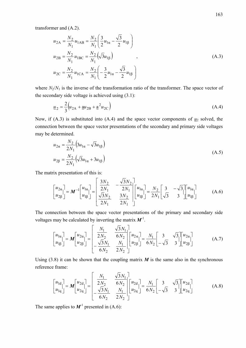
163
transformer and (A.2).
( )
⎟⎟⎠
⎞⎜⎜⎝
⎛−−==
==
⎟⎟⎠
⎞⎜⎜⎝
⎛−==
1β1α1
21CA
1
22C
1β1
21BC
1
2B2
1β1α1
21AB
1
2A2
23
23
3
23
23
uuNNu
NNu
uNN
uNN
u
uuNNu
NNu
, (A.3)
where N2/N1 is the inverse of the transformation ratio of the transformer. The space vector of the secondary side voltage is achieved using (3.1):
( )2C2
2B2A2 aa32 uuuu ++= (A.4)
Now, if (A.3) is substituted into (A.4) and the space vector components of u2 solved, the connection between the space vector presentations of the secondary and primary side voltages may be determined.
( )
( )1β1α1
2β2
1β1α1
2α2
332
332
uuN
Nu
uuN
Nu
+=
−=
(A.5)
The matrix presentation of this is:
⎥⎦
⎤⎢⎣
⎡⎥⎦
⎤⎢⎣
⎡ −=⎥
⎦
⎤⎢⎣
⎡
⎥⎥⎥⎥
⎦
⎤
⎢⎢⎢⎢
⎣
⎡−
=⎥⎦
⎤⎢⎣
⎡=⎥
⎦
⎤⎢⎣
⎡ −
β1
α1
1
2
β1
α1
1
2
1
2
1
2
1
2
β1
α11
β2
α2
3333
223
23
23
23
uu
NN
uu
NN
NN
NN
NN
uu
uu
M (A.6)
The connection between the space vector presentations of the primary and secondary side voltages may be calculated by inverting the matrix M-1.
⎥⎦
⎤⎢⎣
⎡⎥⎦
⎤⎢⎣
⎡
−=⎥
⎦
⎤⎢⎣
⎡
⎥⎥⎥⎥
⎦
⎤
⎢⎢⎢⎢
⎣
⎡
−=⎥
⎦
⎤⎢⎣
⎡=⎥
⎦
⎤⎢⎣
⎡
β2
α2
2
1
β2
α2
2
1
2
1
2
1
2
1
β2
α2
β1
α1
3333
626
363
2uu
NN
uu
NN
NN
NN
NN
uu
uu
M (A.7)
Using (3.8) it can be shown that the coupling matrix M is the same also in the synchronous reference frame:
⎥⎦
⎤⎢⎣
⎡⎥⎦
⎤⎢⎣
⎡
−=⎥
⎦
⎤⎢⎣
⎡
⎥⎥⎥⎥
⎦
⎤
⎢⎢⎢⎢
⎣
⎡
−=⎥
⎦
⎤⎢⎣
⎡=⎥
⎦
⎤⎢⎣
⎡
q2
d2
2
1
q2
d2
2
1
2
1
2
1
2
1
q2
d2
q1
d1
3333
626
363
2uu
NN
uu
NN
NN
NN
NN
uu
uu
M (A.8)
The same applies to M-1 presented in (A.6):

164 Appendix A
⎥⎦
⎤⎢⎣
⎡⎥⎦
⎤⎢⎣
⎡ −=⎥
⎦
⎤⎢⎣
⎡
⎥⎥⎥⎥
⎦
⎤
⎢⎢⎢⎢
⎣
⎡−
=⎥⎦
⎤⎢⎣
⎡=⎥
⎦
⎤⎢⎣
⎡ −
q1
d1
1
2
q1
d1
1
2
1
2
1
2
1
2
q1
d11
q2
d2
3333
223
23
23
23
uu
NN
uu
NN
NN
NN
NN
uu
uu
M (A.9)

165
Appendix B
Simulation model details
This appendix presents some details of MatLab/Simulink simulation models discussed in Chapter 4. In Fig. B.1 a pulse width modulated voltage source inverter (PWM-VSI) model used with the series connected topology (SCT) is presented. The PWM-VSI model consists of a control system, a space vector modulator and hardware of the inverter.
Fig. B.1. PWM-VSI model.
The PWM-VSI models used with the filter connected topology (FCT) and the electrically tuned LC shunt circuit (ETLC) are basically similar to the presented PWM-VSI model. However, there are differences between their control systems as was discussed in Chapter 4. In the modelling of the PWM-VSI of the UPQC it has to be noticed that there are two switching bridges and only one dc-link. This causes slight differences to the inverter hardware model compared to the one shown in Fig. B.1. The simulation model of the inverter hardware shown in Fig. B.1 is shown more closely in Fig. B.2. The model is based on equations presented in Chapter 4.1.
Fig. B.2. Inverter hardware model.
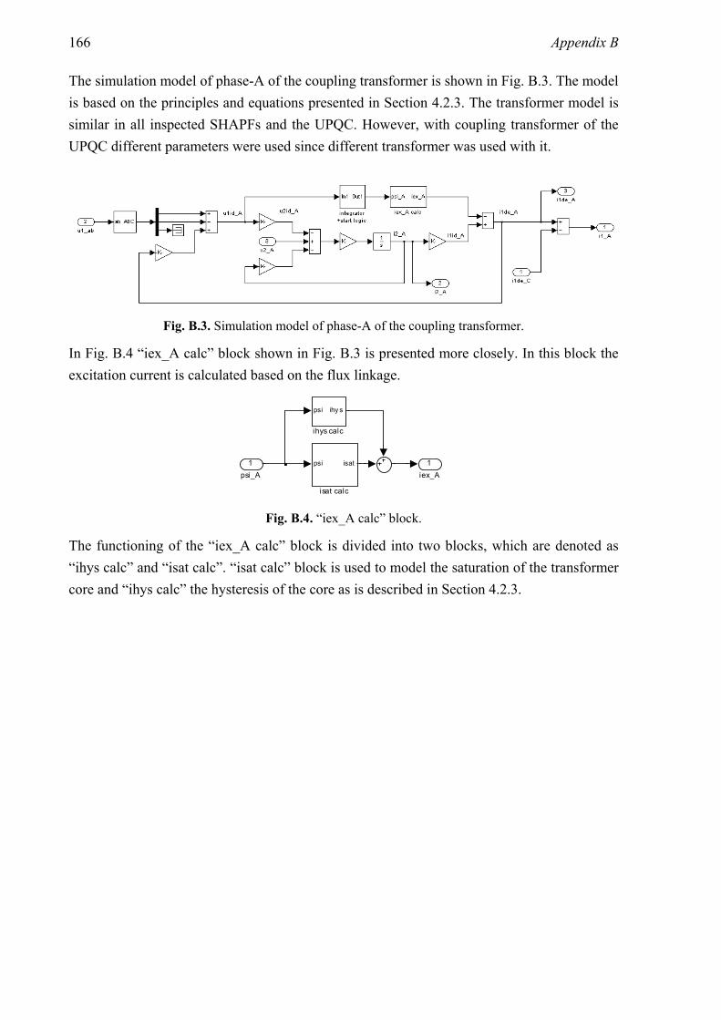
166 Appendix B
The simulation model of phase-A of the coupling transformer is shown in Fig. B.3. The model is based on the principles and equations presented in Section 4.2.3. The transformer model is similar in all inspected SHAPFs and the UPQC. However, with coupling transformer of the UPQC different parameters were used since different transformer was used with it.
Fig. B.3. Simulation model of phase-A of the coupling transformer.
In Fig. B.4 “iex_A calc” block shown in Fig. B.3 is presented more closely. In this block the excitation current is calculated based on the flux linkage.
1iex_A
psi isat
isat calc
psi ihy s
ihys calc
1psi_A
Fig. B.4. “iex_A calc” block.
The functioning of the “iex_A calc” block is divided into two blocks, which are denoted as “ihys calc” and “isat calc”. “isat calc” block is used to model the saturation of the transformer core and “ihys calc” the hysteresis of the core as is described in Section 4.2.3.

167
Appendix C
SHAPF prototypes
The experimental test setup is presented in Fig. C.1.
Fig. C.1. Experimental setup.
The numbered components in the above figure are: 1. Three-phase power supply and a single-phase variac, which was used as a power
supply for the low voltage circuits of the pulse width modulated voltage source inverter (PWM-VSI).
2. ELGAR SW 5250A three-phase power supply, which was used in the unified power quality conditioner (UPQC) tests.
3. Three-phase transformer, which was used as an auxiliary power supply for the PWM-VSI in some series hybrid active power filter (SHAPF) tests.
4. PWM-VSI prototype. 5. Contactor controlled dc-link protection resistor. 6. PC used in communicating with the PWM-VSI microcontroller.
1. 2.
3. 10.
5.
6.
7.
4.
8.
9.
11.
12.
13.

168 Appendix C
7. LC-filter of the series active power filter (SAPF) (second box from the top) and LCL-filter of the parallel active power filter (PAPF).
8. Coupling transformers (2:1 and 10:1). 9. LC shunt circuits tuned for the 5th and 7th harmonic frequencies and high-pass filter
(at the bottom of the stack) and LC shunt circuit used with ETLC (at the top of the stack).
10. Start-up resistor of LC shunt circuits. 11. RL and RC-loads excluding the resistors. 12. Load resistors. 13. Measurement equipment. All SHAPF topologies and the UPQC were built using the same PWM-VSI prototype. Each topology was constructed using the same PWM-VSI, together with other necessary circuit elements. Each topology had its own software, which was uploaded to the microcontroller before the tests. The PWM-VSI prototype is presented in Fig. C.2.
Fig. C.2. PWM-VSI prototype.
1. 2.
3.
4. 6.
7.
8.
9.
10.
11.
5.
12.
13.

169
The numbered components in the above figure are: 1. Supply inductor. 2. Measurement board of the supply currents. 3. Dc-link capacitors. 4. Measurement board of the dc-link voltage. 5. Two IGBT bridges and a diode bridge on a cooler. 6. Measurement boards of the converters output currents. 7. Load voltage measurement board (hidden below the frame). 8. Measurement board of the auxiliary current sensor (measures LC shunt circuit
current in the case of the ETLC and load current in the case of the UPQC) and the measurement board of the supply voltage.
9. Auxiliary current sensor. 10. Two microcontroller boards. 11. Relay boards used to control three-phase contactors. 12. Two boards, which included the driver circuits for the IGBT bridges and power
supplies. Power supplies were used to supply the microcontroller board, the relay board and the measurement boards.
13. Single-phase 230 V / 24 V transformer which was used to feed the power supply circuits.
Microcontroller
The MPC-563 microcontroller made by Motorola was used with the APF prototype. The most important features of the microcontroller are given here (Freescale, 2003).
• 32-bit PowerPCTM single issue RISC processor • Integrated floating-point unit • 32 KB RAM memory • 512 KB flash memory • 5 V I/O-levels • Two time processor units, which both have 16 programmable channels • Modular I/O-system with several submodules • Two A/D conversion units, which both have 16 inputs channels • Serial communication interface • PBGA package with 388 pins • 40 MHz clock frequency

170 Appendix C
Prototypes components and parameters
Those parameters of the SHAPF prototypes, which have not been discussed in Chapter 5 are presented here. In the prototype of the PWM-VSI, SKM 40 GD 123 IGBT modules manufactured by Semikron were used. Each module consists of six IGB transistors. The current and voltage ratings of the module are 40 A / 1200 V. In the dc-link, two series-connected 3.3 mF electrolytic capacitors manufactured by Evox rifa were used. The voltage rating of the series-connected capacitor bank was 1000 V. All transformers and inductors were manufactured by Trafomik. The parameters of each prototype are presented next. The presented resistor values are measured. The inductances of the inductors, except the ones of the load inductor and the commutating inductor, are measured using 50 Hz signal, the amplitude of which is equal to the nominal value of the inductor. The inductance values of the load inductor and the commutating inductor are taken from the type plates. The parameters of the transformers are measured using short-circuit and open-circuit tests. The capacitances of the capacitors, except the one of the load capacitor, are measured. The capacitance of the load capacitor is taken from the type plate. The load parameters are given in Table C.1.
Table C.1. Load parameters.
Parameter Value Capacitance of the load capacitor, Clo 1.1 mF Inductance of the load inductor, Llo 10.0 mH Inductance of the commutating inductor, Lco 2.3 mH Resistance of the load resistor (SCT, FCT and ETLC), Rlo 72 Ω / 212 Ω Resistance of the load resistor (UPQC), Rlo 104 Ω / 206 Ω
The main circuit parameters of the SCT and the FCT are presented in Table C.2.

171
Table C.2. Main circuit parameters of the SCT and the FCT.
Parameter Value Capacitance of the capacitor of the LC shunt circuit tuned for the 5th harmonic frequency, C5 20.4 μFCapacitance of the capacitor of the LC shunt circuit tuned for the 7th harmonic frequency, C7 16.3 μF Capacitance of the high-pass filter capacitor, Chp 16.8 μF Capacitance of the LC-filter capacitor, Csf 0.3 μF Dc-resistance of the high-pass filter inductor, Rhpdc 206 mΩ Dc-resistance of the inductor of the LC shunt circuit tuned for 5th harmonic component, R5dc 441 mΩ Dc-resistance of the inductor of the LC shunt circuit tuned for 7th harmonic component, R7dc 323 mΩ Dc-resistance of the LC-filter inductor, Rsfdc 72 mΩ Dc-resistance of the supply inductor, Rsupdc 57 mΩ Inductance of the high-pass filter inductor, Lhp 6.2 mH Inductance of the inductor of the LC shunt circuit tuned for the 5th harmonic frequency, L5 23.7 mH Inductance of the inductor of the LC shunt circuit tuned for the 7th harmonic frequency, L7 15.4 mH Inductance of the LC-filter inductor, Lsf 5.3 mH Inductance of the supply inductor, Lsup 3.7 mH (3.7 %)Leakage inductance of the primary side of the coupling transformer, L1 6.1 mH Leakage inductance of the secondary side of the coupling transformer, L2 61 μH Resistance of the primary side of the coupling transformer, R1 5.6 Ω Resistance of the secondary side of the coupling transformer, R2 56 mΩ Resistance of the high-pass filter resistor, Rhp 10 Ω Transformation ratio of the coupling transformer 10:1
The main circuit parameters of the ETLC are presented in Table C.3.
Table C.3. Main circuit parameters of ETLC.
Parameter Value Capacitance of the LC-filter capacitor, Csf 0.3 μFCapacitance of the LC shunt circuit capacitor, Cf 20.5 μF Dc-resistance of the LC-filter inductor, Rsfdc 129 mΩ Dc-resistance of the LC shunt circuit inductor, Rfdc 348 mΩ Dc-resistance of the supply inductor, Rsupdc 57 mΩ Inductance of the LC-filter inductor, Lsf 14.9 mH Inductance of the LC shunt circuit inductor, Lf 18.1 mH Inductance of the supply inductor, Lsup 3.7 mH (3.7 %)Leakage inductance of the primary side of the coupling transformer, L1 6.1 mH Leakage inductance of the secondary side of the coupling transformer, L2 61 μH Resistance of the primary side of the coupling transformer, R1 5.6 Ω Resistance of the secondary side of the coupling transformer, R2 56 mΩ Transformation ratio of the coupling transformer 10:1

172 Appendix C
The main circuit parameters of the UPQC are presented in Table C.4.
Table C.4. Main circuit parameters of the UPQC.
Parameter Value Capacitance of the PAPF LCL-filter capacitor, Cpf 5 μF Capacitance of the SAPF LC-filter capacitor, Csf 1 μF Dc-resistance of the PAPF LCL-filter inductor, Rpmdc 33 mΩ Dc-resistance of the PAPF LCL-filter inductor, Rpfdc 69 mΩ Dc-resistance of the SAPF LC-filter inductor, Rsfdc 72 mΩ Inductance of the PAPF LCL-filter inductor, Lpm 1.2 mH Inductance of the PAPF LCL-filter inductor, Lpf 5.2 mH Inductance of the SAPF LC-filter inductor, Lsf 5.3 mH Inductance of the supply, Lsup 0.1 mH Leakage inductance of the primary side of the coupling transformer, L1 863 μH Leakage inductance of the secondary side of the coupling transformer, L2 216 μH Resistance of the PAPF LCL-filter resistor, Rpm 100 Ω Resistance of the primary side of the coupling transformer, R1 468 mΩ Resistance of the secondary side of the coupling transformer, R2 117 mΩ Resistance of the supply, Rsup 30 mΩ Transformation ratio of the coupling transformer 2:1

173
Appendix D
Variation of the load current and load voltage harmonics
In the simulations of this work the same load current waveform achieved from the prototype measurements is used as an input of the simulation models with all SHAPF topologies and the UPQC. This is done in order to simplify the simulation models and to make their process times reasonable. However, since this was done, it had to be assumed that the load current is independent on the load voltage, i.e. the harmonic content of the load current does not depend on the used filter topology. In reality this is not true, but in certain conditions it is a reasonable approximation. The dependency of the harmonic contents of the load voltage and load current on the used SHAPF topology is examined in this appendix. The examination is made in the cases of the RL- and RC-type nonlinear loads, which are used in this work. Both of these loads consist of a three-phase diode rectifier. In the RL-type nonlinear load the inductor and the resistor are connected in series on the dc-side of the diode rectifier and in the case of the RC-type nonlinear load the dc-side load consists of the parallel connected resistor and capacitor.
RL-type nonlinear load
Table D.1 shows the harmonic content of the load current in three cases. First, only the load is connected to the supply. In the supply branch 3.7 mH supply inductor is used. Second, the passive filters of the SCT/FCT are connected in parallel with the load. The measurement results of the SCT and the FCT are given in the same column, since the same passive filters were used with the SCT and FCT. Third, the passive filters of the ETLC are connected in parallel with the load.
Table D.2 presents the harmonic contents of the load current with different SHAPF topologies. These results are achieved with different topologies in cases where the LC-filter is, and is not, used in the output of the PWM-VSI. In addition to this, in the case of the ETLC the measurement results are also shown in the case where the control system that applies active resistance Ract in addition to the active reactances Xact,n, is used. The figures shown in Table D.2 correspond to the measurement results presented in Table 6.4, i.e. the results of these tables are achieved using the same parameters.
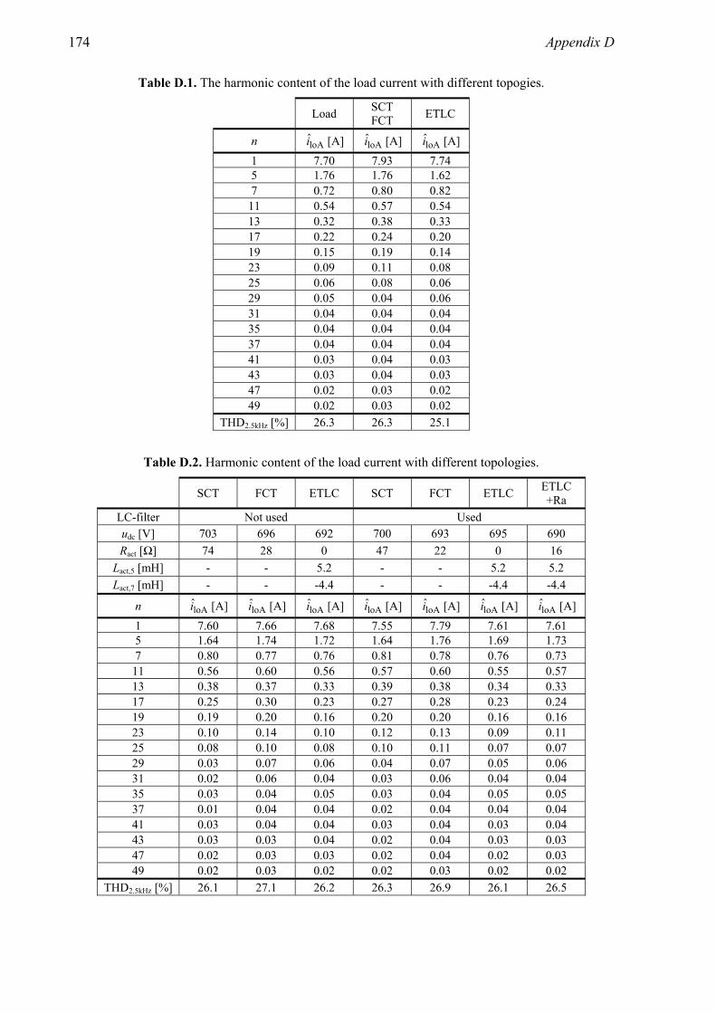
174 Appendix D
Table D.1. The harmonic content of the load current with different topogies.
Load SCT FCT ETLC
n Aloi [A] Aloi [A] Aloi [A] 1 7.70 7.93 7.745 1.76 1.76 1.62 7 0.72 0.80 0.82
11 0.54 0.57 0.54 13 0.32 0.38 0.33 17 0.22 0.24 0.20 19 0.15 0.19 0.14 23 0.09 0.11 0.08 25 0.06 0.08 0.06 29 0.05 0.04 0.06 31 0.04 0.04 0.04 35 0.04 0.04 0.04 37 0.04 0.04 0.04 41 0.03 0.04 0.03 43 0.03 0.04 0.03 47 0.02 0.03 0.02 49 0.02 0.03 0.02
THD2.5kHz [%] 26.3 26.3 25.1
Table D.2. Harmonic content of the load current with different topologies.
SCT FCT ETLC SCT FCT ETLC ETLC +Ra
LC-filter Not used Used udc [V] 703 696 692 700 693 695 690 Ract [Ω] 74 28 0 47 22 0 16
Lact,5 [mH] - - 5.2 - - 5.2 5.2 Lact,7 [mH] - - -4.4 - - -4.4 -4.4
n Aloi [A] Aloi [A] Aloi [A] Aloi [A] Aloi [A] Aloi [A] Aloi [A] 1 7.60 7.66 7.68 7.55 7.79 7.61 7.61 5 1.64 1.74 1.72 1.64 1.76 1.69 1.73 7 0.80 0.77 0.76 0.81 0.78 0.76 0.73
11 0.56 0.60 0.56 0.57 0.60 0.55 0.57 13 0.38 0.37 0.33 0.39 0.38 0.34 0.33 17 0.25 0.30 0.23 0.27 0.28 0.23 0.24 19 0.19 0.20 0.16 0.20 0.20 0.16 0.16 23 0.10 0.14 0.10 0.12 0.13 0.09 0.11 25 0.08 0.10 0.08 0.10 0.11 0.07 0.07 29 0.03 0.07 0.06 0.04 0.07 0.05 0.06 31 0.02 0.06 0.04 0.03 0.06 0.04 0.04 35 0.03 0.04 0.05 0.03 0.04 0.05 0.05 37 0.01 0.04 0.04 0.02 0.04 0.04 0.04 41 0.03 0.04 0.04 0.03 0.04 0.03 0.04 43 0.03 0.03 0.04 0.02 0.04 0.03 0.03 47 0.02 0.03 0.03 0.02 0.04 0.02 0.03 49 0.02 0.03 0.02 0.02 0.03 0.02 0.02
THD2.5kHz [%] 26.1 27.1 26.2 26.3 26.9 26.1 26.5

175
Based on these results it can be seen that the harmonic content of the load current is almost the same in all cases. Tables D.3 and D.4 present the harmonic contents of the phase-A load voltage in the same cases where the harmonic contents of the load current were presented in Tables D.1 and D.2.
Table D.3. Harmonic content of the load voltage with different topologies.
Load SCT FCT ETLC
n Alou [V] Alou [V] Alou [V]
1 326.98 338.74 334.635 8.83 6.34 17.09 7 6.59 3.29 5.45
11 6.31 4.84 4.49 13 4.46 3.54 3.99 17 3.68 2.50 2.92 19 2.78 1.67 2.22 23 2.00 1.12 1.56 25 1.63 1.14 1.23 29 1.64 0.51 1.48 31 1.29 0.51 1.08 35 1.44 0.82 1.14 37 1.11 0.36 1.04 41 1.34 0.45 0.99 43 1.02 0.49 1.02 47 0.86 0.32 0.77 49 0.93 0.33 0.74
THD2.5kHz [%] 4.6 3.0 5.9

176 Appendix D
Table D.4. Harmonic content of the load voltage with different topologies.
SCT FCT ETLC SCT FCT ETLC ETLC +Ra
LC-filter Not used Used udc [V] 703 696 692 700 693 695 690 Ract [Ω] 74 28 0 47 22 0 16
Lact,5 [mH] - - 5.2 - - 5.2 5.2 Lact,7 [mH] - - -4.4 - - -4.4 -4.4
n Alou [V] Alou [V] Alou [V] Alou [V] Alou [V] Alou [V] Alou [V]
1 331.69 333.70 330.49 330.65 333.67 330.37 330.32 5 9.52 2.09 4.30 9.45 2.77 4.43 3.54 7 3.24 1.32 2.39 3.25 1.50 2.67 1.11
11 6.22 3.13 5.45 5.92 3.65 5.29 5.99 13 4.07 2.22 3.84 3.75 2.70 3.89 4.17 17 2.69 2.70 3.15 2.40 3.01 3.05 3.81 19 1.97 2.43 2.67 1.82 2.58 2.75 3.02 23 1.10 2.37 1.87 0.94 2.27 1.79 2.26 25 0.87 1.98 1.62 0.73 1.76 1.63 1.89 29 0.21 1.19 1.22 0.44 1.22 1.17 1.43 31 0.35 0.95 0.98 0.46 0.99 1.00 1.12 35 1.66 1.16 1.54 0.38 1.06 1.22 1.47 37 0.68 0.73 1.11 0.17 0.70 1.10 1.00 41 0.63 0.71 1.09 0.41 0.65 1.00 1.23 43 0.50 0.47 1.14 0.30 0.57 1.12 1.06 47 0.43 0.60 0.85 0.39 0.47 0.77 1.00 49 0.32 0.59 0.79 0.38 0.55 0.87 0.90
THD2.5kHz [%] 4.1 2.2 3.1 3.9 2.4 3.1 3.2
If the harmonic contents of the load voltage are examined in cases of different topologies, it can be seen that there are relatively quite big differences between them. Based on this it can be stated that although the harmonic content of the load voltage is dependent on the used SHAPF topology, the harmonic content of the load current is quite independent on it. Therefore, it can be assumed that the harmonic content of the load current is independent on the load voltage variations. Because of this it is justified to use the measured load current waveform as an input of the simulation models of all SHAPFs in the case of the RL-type nonlinear load.
RC-type nonlinear load
In Tables D.5 – D.8 the harmonic contents of the load current and load voltage are presented in the case of RC-type nonlinear load in similar cases to those presented in Tables D.1 – D.4 in the case of RL-type nonlinear load. Tables D.5 and D.7 present the harmonic contents of the load current and the load voltage in cases where only the load is connected to the supply or only the passive filters of the SHAPF topologies are used in the current harmonics filtering. Tables D.6 and D.8 present the harmonic contents of the load current and the load voltage in the case of different SHAPF topologies. The figures shown in Tables D.6 and D.8 are achieved using the same parameters as the measurement results presented in Table 6.11.

177
Table D.5. Harmonic content of the load current with different topologies.
Load SCT FCT ETLC
n Aloi [A] Aloi [A] Aloi [A] 1 7.81 7.76 7.545 2.94 3.33 2.21 7 0.97 1.23 0.60
11 0.54 0.50 0.53 13 0.26 0.20 0.28 17 0.21 0.23 0.17 19 0.16 0.14 0.15 23 0.10 0.13 0.09 25 0.09 0.09 0.08 29 0.06 0.06 0.06 31 0.07 0.07 0.04 35 0.03 0.03 0.04 37 0.04 0.04 0.03 41 0.04 0.02 0.03 43 0.03 0.03 0.03 47 0.03 0.03 0.02 49 0.02 0.02 0.02
THD2.5kHz [%] 40.7 46.6 31.7
Table D.6. Harmonic content of the load current with different topologies.
SCT FCT ETLC SCT FCT ETLC ETLC +Ra
LC-filter Not used Used udc [V] 702 689 695 697 686 696 690 Ract [Ω] 62 14 0 42 11 0 4
Lact,5 [mH] - - 5.2 - - 5.2 5.2 Lact,7 [mH] - - -4.4 - - -4.4 -4.4
n Aloi [A] Aloi [A] Aloi [A] Aloi [A] Aloi [A] Aloi [A] Aloi [A] 1 7.69 7.72 7.49 7.65 7.70 7.49 7.415 2.88 3.76 3.18 2.85 3.57 3.12 3.18 7 0.74 1.80 1.11 0.71 1.66 1.08 1.25
11 0.50 0.55 0.48 0.51 0.54 0.48 0.53 13 0.12 0.27 0.21 0.11 0.27 0.20 0.21 17 0.21 0.23 0.20 0.22 0.23 0.21 0.21 19 0.12 0.14 0.13 0.11 0.15 0.13 0.14 23 0.11 0.14 0.11 0.11 0.14 0.11 0.12 25 0.08 0.09 0.08 0.09 0.10 0.09 0.09 29 0.04 0.08 0.05 0.07 0.08 0.05 0.07 31 0.07 0.07 0.06 0.05 0.07 0.05 0.05 35 0.03 0.05 0.04 0.03 0.05 0.04 0.03 37 0.04 0.05 0.04 0.03 0.05 0.04 0.03 41 0.02 0.03 0.03 0.02 0.03 0.03 0.03 43 0.03 0.04 0.02 0.02 0.04 0.03 0.02 47 0.02 0.02 0.03 0.01 0.03 0.03 0.02 49 0.02 0.03 0.02 0.02 0.03 0.02 0.02
THD2.5kHz [%] 39.5 54.9 45.8 39.2 52.0 44.9 47.1

178 Appendix D
Table D.7. Harmonic content of the load voltage with different topologies.
Load SCT FCT ETLC
n Alou [V] Alou [V] Alou [V]
1 326.68 338.21 334.475 13.42 10.90 22.36 7 5.35 3.77 2.97
11 6.02 3.76 4.13 13 3.21 1.79 2.71 17 3.59 2.32 2.68 19 2.81 1.30 2.54 23 2.26 1.24 1.49 25 2.21 1.12 1.66 29 1.53 0.57 1.48 31 1.46 0.57 1.14 35 1.39 0.87 1.34 37 1.02 0.59 0.99 41 1.29 0.22 0.90 43 0.91 0.52 1.09 47 1.08 0.32 0.83 49 1.02 0.09 0.77
THD2.5kHz [%] 5.3 3.8 7.1
Table D.8. Harmonic content of the load voltage with different topologies.
SCT FCT ETLC SCT FCT ETLC ETLC +Ra
LC-filter Not used Used udc [V] 702 689 695 697 686 696 690 Ract [Ω] 62 14 0 42 11 0 4
Lact,5 [mH] - - 5.2 - - 5.2 5.2 Lact,7 [mH] - - -4.4 - - -4.4 -4.4
n Alou [V] Alou [V] Alou [V] Alou [V] Alou [V] Alou [V] Alou [V]
1 331.21 333.63 329.73 329.60 332.46 329.63 330.03 5 15.30 6.12 9.26 15.28 6.86 9.23 8.59 7 2.74 2.80 2.16 2.46 3.15 2.70 2.97
11 4.42 4.04 4.71 4.36 4.25 4.68 5.21 13 1.32 2.59 2.53 1.13 2.57 2.51 2.48 17 2.28 2.75 2.81 2.13 2.60 2.75 3.19 19 1.02 1.56 2.03 0.98 1.80 2.09 2.23 23 1.04 1.99 1.99 0.88 1.75 1.96 2.20 25 0.85 1.43 1.79 0.82 1.45 1.88 1.93 29 0.46 1.00 1.32 0.42 1.05 1.23 1.44 31 0.88 1.05 1.49 0.71 1.07 1.40 1.50 35 0.55 1.07 1.09 0.47 1.00 1.03 1.27 37 0.67 0.64 1.06 0.57 0.83 1.14 1.17 41 0.39 0.55 0.83 0.24 0.50 0.88 0.96 43 0.53 0.46 0.77 0.40 0.55 0.81 0.99 47 0.33 0.40 0.88 0.37 0.35 0.74 0.97 49 0.30 0.41 0.65 0.21 0.37 0.64 0.56
THD2.5kHz [%] 5.0 2.9 3.7 5.0 3.1 3.7 3.8

179
Based on the measurement results it can be seen that the harmonic content of the load voltage is dependent on the used SHAPF topology also with the RC-type nonlinear load. However, in this case it can be seen that also the harmonic content of the load current differs in cases where only the load is connected and where the different SHAPF topologies are used. This is the case especially with the FCT. Based on this it can be stated that the load voltage variations have an influence on the harmonic content of the load current in the case of the RC-type nonlinear load. Therefore, in cases where the measured load current waveform of the RC-type nonlinear load is used as an input of the simulation models, an error is produced in the simulation results. This error is greatest in the case of the FCT.