Brigham Young UniversityBYU ScholarsArchive

Faculty Publications

2019-8

Takeoff and Performance Tradeoffs of RetrofitDistributed Electric Propulsion for UrbanTransportKevin MooreBrigham Young University, moorekevin711@gmail.com

Andrew NingBrigham Young University, aning@byu.edu

Follow this and additional works at: https://scholarsarchive.byu.edu/facpubPart of the Mechanical Engineering Commons

Original Publication CitationMoore, K., and Ning, A., “Takeoff and Performance Tradeoffs of Retrofit Distributed ElectricPropulsion for Urban Transport,” Journal of Aircraft, Aug. 2019. doi:10.2514/1.C035321

This Peer-Reviewed Article is brought to you for free and open access by BYU ScholarsArchive. It has been accepted for inclusion in FacultyPublications by an authorized administrator of BYU ScholarsArchive. For more information, please contact scholarsarchive@byu.edu,ellen_amatangelo@byu.edu.

BYU ScholarsArchive CitationMoore, Kevin and Ning, Andrew, "Takeoff and Performance Tradeoffs of Retrofit Distributed Electric Propulsion for UrbanTransport" (2019). Faculty Publications. 3248.https://scholarsarchive.byu.edu/facpub/3248

Takeoff and Performance Tradeoffs of Retrofit Distributed

Electric Propulsion for Urban Transport

Kevin R. Moore∗ and Andrew Ning†

Brigham Young University, Provo, UT, 84602, USA

While vertical takeoff and landing aircraft have shown promise for urban air transport,

distributed electric propulsion on existing aircraft may offer immediately implementable alter-

natives. Distributed electric propulsion could potentially decrease takeoff distances enough to

enable thousands of potential inter-city runways. This conceptual study explores the effects

of a retrofit of open-bladed electric propulsion units. To model and explore the design space

we use blade element momentum method, vortex lattice method, linear-beam finite element

analysis, classical laminate theory, composite failure, empirically-based blade noise modeling,

motor and motor-controller mass models, and gradient-based optimization. With liftoff time

of seconds and the safe total field length for this aircraft type undefined, we focused on the

minimum conceptual takeoff distance. We found that 16 propellers could reduce the takeoff

distance by over 50% compared to the optimal 2 propeller case. This resulted in a conceptual

minimum takeoff distance of 20.5 meters to clear a 50 ft (15.24 m) obstacle. We also found that

when decreasing the allowable noise by approximately 10 dBa, the 8 propeller case performed

the best with a 43% reduction in takeoff distance compared to the optimal 2 propeller case.

This resulted in a noise-restricted conceptual minimum takeoff distance of 95 meters.

I. IntroductionIn early aircraft designs, distributed propulsion was used more out of necessity than deliberate choice. Designs such

as the Dornier Do X in 1929, the Hughes H-4 Hercules in 1947, and many other large aircraft before the jet age, were

constrained by the available propulsion units of the time [1]. With the dawn of the jet age, aircraft began to use fewer but

larger engines. However, some distributed and blended wing jet concepts were explored as early as 1954 [2]. During the

push for high altitude long endurance (HALE) aircraft design, distributed electric propulsion (DEP) emerged as a viable

option with NASA’s Pathfinder in 1983 [3]. In 1988, NASA produced several concepts including distributed propulsion

with the intention of lift augmentation [4], which evolved until the Helios’ destruction in 2003 [5]. In the 2000s, a third

wave of aeronautics began to emerge, termed by NASA as on demand mobility (ODM) [6], or unscheduled aircraft

services. Within ODM, two applications have begun to be targeted: thin-haul commuters and urban air taxis [7].

Fig. 1 NASA X-57 thin-haul concept aircraft illustration∗ showing the mid span DEP propellers in the folded

cruise position.

∗Masters Student, Department of Mechanical Engineering, AIAA Student Member†Assistant Professor, Department of Mechanical Engineering, AIAA Senior Member∗Image reprinted from “NASA Electric Research Plane Gets X Number, New Name", by A. Beutel, 2017, Retrieved from

https://www.nasa.gov/press-release/nasa-electric-research-plane-gets-x-number-new-name. Public Domain Credit: NASA

1

Thin-haul commuters, the first ODM application, are aircraft designed to fly routes not justifiable by large airlines.

An example concept emerged in 2014 when NASA partnered with Joby Aviation and Empirical Systems Aerospace

to use the Leading Edge Asynchronous Propeller Technology (LEAPTech) as a test bed for distributed propulsion

research [8]. Additionally, in 2016, NASA announced the X-57 Maxwell short haul commuter (see fig. 1) with goals to

reduce the energy required for cruise by 4.8x without sacrificing cruise speed or takeoff distance [9]. Since the X-57,

there has been a significant increase in the amount of research regarding DEP for thin-haul commuters in areas such as

economics[10], multidisciplinary modeling requirements [11], wing aerodynamic analysis [8, 9, 12], motor design [13],

avionics [14], hybrid propulsion [15], trajectory thermal considerations [16], certification and landing safety [17] and

large scale multidisciplinary optimization of design and trajectory [7].

Urban air taxis, the second ODM application, are aircraft designed for 2-6 passengers and distances less than 100

miles [18]. Though there is significant infrastructure required to adopt this type of transportation, there is potential

for competitive operating costs [19]. The economic possibilities have driven the development of a variety of concepts

including tilt rotor, multi-rotor, and tilting ducted fans. The concept of urban air transport with conventional small

fixed-wing aircraft as opposed to vertical takeoff and landing aircraft has been previously explored [20]. However, the

concept of using distributed electric propulsion to shorten the runway distance is relatively recent. In the predecessor to

this work [21], we used a propeller-on-wing aerodynamic model and electric component performance modeling to show

an 80% reduction in takeoff rolling distance using an optimal distributed electric propulsion design as opposed to an

optimal two-propeller electric configuration. More recently, Courtin et al. [22] conducted a feasibility analysis of the

STOL concept for urban air transport with the geometric programming (GP) method. They took a broad approach

to the STOL urban air transport problem including takeoff rolling distance, landing distance, wing spar sizing using

root bending moment, propulsion effects via 2D jets, and lift augmentation using a momentum balance. According to

the study, runway lengths need only be less than 150 m (500 ft) to have feasible DEP aircraft access to thousands of

potential locations in cities such as Dallas and Chicago.

This work builds upon previous work with the following contributions: First, we integrate a wide range of

multidisciplinary models and constraints including propeller aerostructural coupling, propeller noise, aircraft takeoff

path dynamics, propeller on wing interactions, power conversion efficiency, and electrical component mass. Second,

we include model modifications that allow for efficient gradient based optimization using a new method for smooth

gradients with respect to propeller on wing interactions. Third, we present several case studies looking at the sensitivity

to a few critical parameters that help better understand the design tradeoffs of a short takeoff fixed wing aircraft in urban

transport applications.

II. Model DescriptionIn this section, models relating to propeller and wing aerodynamics, propeller noise, propeller aerostructural, and

electrical component modeling are outlined. These include blade element momentum theory, airfoil preprocessing, BPM

(Brooks, Pope, and Marcolini) noise modeling, composite structures, vortex lattice method, propeller on wing interaction

modeling, electric motor performance and mass, motor controller mass, and battery mass. Several verification and

validation cases are also presented.

A. Propeller Aerodynamics

We use CCBlade, an open source blade element momentum (BEM) code formulated to give guaranteed convergence

and in turn allow for a continuously differentiable output [23].† It includes a non-normal inflow correction which allows

us to mount the props in line with the wing and include the angle of attack (AOA) of the wing as the inflow angle to the

prop. For atmospheric properties we use NASA’s 1976 Standard Atmosphere Model‡ [24]. From CCBlade we extract

axial and tangential induced flow distributions to be able to compute the propeller wake influence on the wing. This

BEM formulation uses 2D airfoil data to calculate the induction factors for each annular disk of the propeller including

Prandtl hub and tip loss correction factors [25]. To properly model the induced wake velocity in BEM formulation, the

tip loss factors must be included in the output induced velocities.

Propeller wakes generally reach their far-field values within approximately one rotor radius [26]. In this conceptual

design study, we model the propeller as being removed one radius or more from the wing for the far-field values to

be applied on the wing. This removes the need to model slipstream contraction and the associated changes in wing

†CCBlade.jl on BYU FLOW Lab GitHub https://github.com/byuflowlab/CCBlade.jl‡BYU FLOW Lab GitHub Atmosphere.jl https://github.com/byuflowlab/Atmosphere.jl

2

angle of attack and spanwise flow that would otherwise be present with a propeller closer than one radius to the wing.

This configuration is similar to tests conducted by Veldhuis and Epema [27, 28]. Additionally, in their experimental

results, not all of the tangentially induced velocity from the propeller is applied normal to the wing chordline. This swirl

reduction factor (SRF) is approximately 0.5 [27] for a propeller in line with the wing chord. Similar to that done by

Veldhuis [27], we model the annular contraction as being fixed at the wake center with the contraction compounding to

the edge of the stream tube. Applying the fully developed wake on the wing has the advantage of removing the need to

model changes in the wing angle of attack due to wake contraction.

1. Airfoil Pre-computation

Blade element momentum theory is dependent on accurate airfoil data for accurate propeller performance prediction.

To calculate the airfoil data, we use XFOIL§ to run the Eppler 212 airfoil for thirteen Reynolds numbers ranging from

5 × 104 to 1 × 108, five Mach numbers ranging from 0 to 0.8, and fifty-one angles of attack ranging between negative

and positive stall (approximately negative 10◦ to positive 20◦, depending on the Reynolds and Mach number).

We use Airfoilpreppy¶ [29] to model the stall delay experienced by local sections on rotating blades. This code

applies the rotational correction on lift by Du et al. [30] and drag by Eggers et al. [31] as well as extrapolation to high

angles of attack by Viterna et al. [32].

2. Propeller Performance Comparison

To validate that the BEM code with XFOIL airfoil data calculation was consistent with Epema’s published

experimental cases [28], we compared his published experimental results with our computational model of his setup.

The results for a constant RPM and varying freestream are seen in fig. 2. Since the 2D airfoil data includes stall, the

modeled effects of stall can be seen on the 3D propeller performance for very low advance ratios. The more linear

regions at the lowest advance ratios are comprised of post-stall angles of attack calculated by the Viterna extrapolation.

AirfoilData

MomentumBalance

25°

35°30°

Pitch

Fig. 2 Comparison of propeller efficiency with data collected by Epema [28] and our BEM model using XFOIL

airfoil data. A maximum error of 5% can be seen in the normal regions of operation.

B. Propeller Noise

In our early versions of this work [21] we used propeller tip speed as a surrogate for noise. We showed that the

takeoff performance of a DEP STOL aircraft was much less affected using tip speed constraints than what we show in

this current work using semi-experimental blade noise. While tip speed captures the magnitude change in noise for a set

number of propellers, it is not enough to enable comparison of noise between aircraft designs with different numbers of

propellers and the associated blade design changes. In this study we model propeller noise using code‖ developed and

validated by Tingey [33], which uses acoustic modeling techniques by Brooks, Pope, and Marcolini (referred to as the

BPM equations) [34, 35].

§Xfoil.jl on BYU FLOW Lab GitHub https://github.com/byuflowlab/Xfoil.jl¶AirfoilPreppy on BYU FLOW Lab GitHub https://github.com/byuflowlab/AirfoilPreppy‖BPM.jl on BYU FLOW Lab GitHub https://github.com/byuflowlab/BPM.jl

3

Figure 3 shows a graphical representation of the A-weighted noise profile for an example 8 propeller case in climb

at 50 ft with respect to a ground observer. Because this is a comparative conceptual study, we use this semi-empirical

noise model as an approximate calculation for the major components of propeller noise. More detailed use of this model

would require calibration and validation specific to the application, as well as other forms of noise generated by the rest

of the aircraft such as from the wing, fuselage, electric motors, and motor controllers. However, this model captures the

main portion of the total noise generation of an electric aircraft enabling us to make a better a comparison between

designs with different numbers of propellers, blades, and blade geometry.

Fig. 3 Noise profile of example 8 propeller case in climb at 50 ft with respect to a ground observer. (Airframe

included for reference.)

C. Composite Structures

Since our objective is to minimize takeoff distance, the propellers will be subject to very high loading to achieve the

thrust required on takeoff. To achieve a more realistic total design, we need to include the structural constraints and their

effects on the aerodynamic design. These constraints ensure that the blade design and structure meets failure criteria as

well as minimum and maximum composite thicknesses. A by-product of this is that the total propeller mass can be more

accurately predicted, which in some cases can be as high as 6% of the allowable propulsion and battery mass.

1. Propeller Blade Composite Layup

The composite layup for the propellers is defined as a shell with two ply types: unidirectional (or uni) carbon prepreg

along the blade span and bidirectional weave (or weave) oriented at 45◦. To enable gradient-based optimization for this

conceptual study, the plies are modeled with continuous thicknesses.

We use PreComp∗∗ to calculate the span-variant sectional properties of the shell, which include mass, stiffnesses,

and inertias. From the distributed mass, we calculate each blade mass with trapezoidal integration and scale it according

to the number of propellers and blades. PreComp also calculates the structural centers of shear, mass, and tension which

are needed to transform the aerodynamic forces from the aerodynamic center into the structural frame of reference. The

relative distances between the structural centers and the aerodynamic center are used to transform the aerodynamic

forces at the aerodynamic center of each section, calculated by BEM, into the structural frame of reference.

2. Linear Finite Element Analysis

With the propeller blade distributed stiffnesses calculated from PreComp, we use linear beam finite element

theory [36],†† to model the blade. This is done with the beam fixed at the hub and the propeller aerodynamic loads

∗∗PreComp.jl on BYU FLOW Lab GitHub https://github.com/byuflowlab/PreComp.jl††BeamFEA.jl on BYU FLOW Lab GitHub https://github.com/byuflowlab/BeamFEA.jl

4

distributed along the blade. For this study, strains are calculated at 10 evenly spaced points around the airfoils at 8

sections along the blade using a thin shell approach.

3. Composite Frame of Reference Stress

To calculate stresses in the composite frame and in turn first ply failure, we use a thin shell calculation with the

composite centerline strain for all layers. Calculating composite stress in the composite frame of reference is a multi-step

process including calculating the shear strain and laminate stress in the beam frame of reference, then transforming the

stress into the ply frame of reference [37].

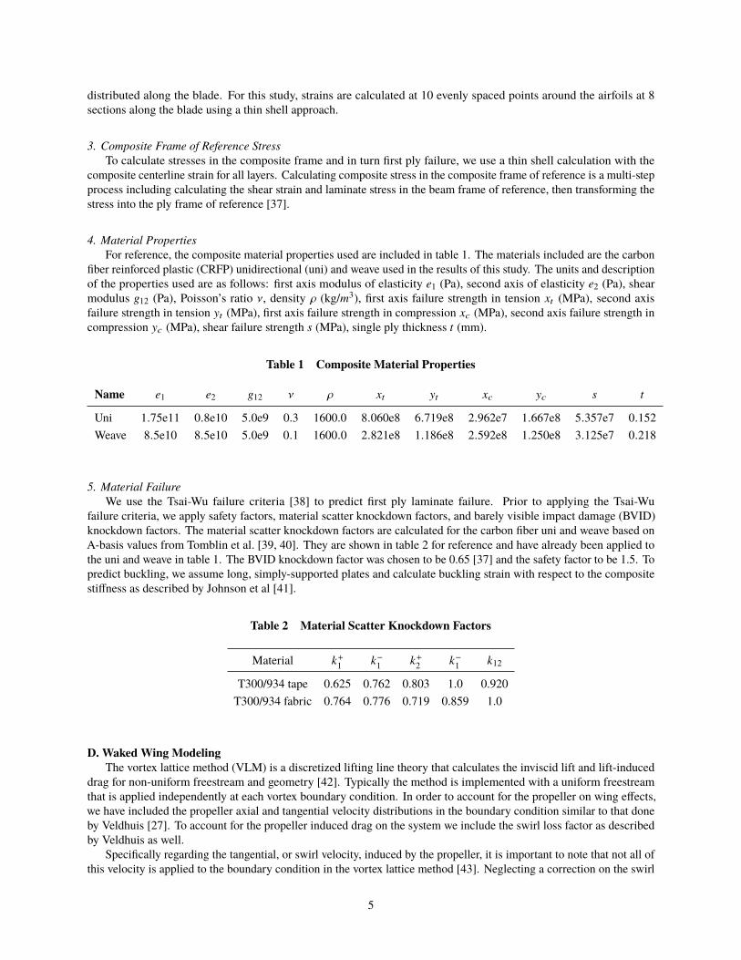
4. Material Properties

For reference, the composite material properties used are included in table 1. The materials included are the carbon

fiber reinforced plastic (CRFP) unidirectional (uni) and weave used in the results of this study. The units and description

of the properties used are as follows: first axis modulus of elasticity e1 (Pa), second axis of elasticity e2 (Pa), shear

modulus g12 (Pa), Poisson’s ratio ν, density ρ (kg/m3), first axis failure strength in tension xt (MPa), second axis

failure strength in tension yt (MPa), first axis failure strength in compression xc (MPa), second axis failure strength in

compression yc (MPa), shear failure strength s (MPa), single ply thickness t (mm).

Table 1 Composite Material Properties

Name e1 e2 g12 ν ρ xt yt xc yc s t

Uni 1.75e11 0.8e10 5.0e9 0.3 1600.0 8.060e8 6.719e8 2.962e7 1.667e8 5.357e7 0.152

Weave 8.5e10 8.5e10 5.0e9 0.1 1600.0 2.821e8 1.186e8 2.592e8 1.250e8 3.125e7 0.218

5. Material Failure

We use the Tsai-Wu failure criteria [38] to predict first ply laminate failure. Prior to applying the Tsai-Wu

failure criteria, we apply safety factors, material scatter knockdown factors, and barely visible impact damage (BVID)

knockdown factors. The material scatter knockdown factors are calculated for the carbon fiber uni and weave based on

A-basis values from Tomblin et al. [39, 40]. They are shown in table 2 for reference and have already been applied to

the uni and weave in table 1. The BVID knockdown factor was chosen to be 0.65 [37] and the safety factor to be 1.5. To

predict buckling, we assume long, simply-supported plates and calculate buckling strain with respect to the composite

stiffness as described by Johnson et al [41].

Table 2 Material Scatter Knockdown Factors

Material k+

1k−1

k+

2k−1

k12

T300/934 tape 0.625 0.762 0.803 1.0 0.920

T300/934 fabric 0.764 0.776 0.719 0.859 1.0

D. Waked Wing Modeling

The vortex lattice method (VLM) is a discretized lifting line theory that calculates the inviscid lift and lift-induced

drag for non-uniform freestream and geometry [42]. Typically the method is implemented with a uniform freestream

that is applied independently at each vortex boundary condition. In order to account for the propeller on wing effects,

we have included the propeller axial and tangential velocity distributions in the boundary condition similar to that done

by Veldhuis [27]. To account for the propeller induced drag on the system we include the swirl loss factor as described

by Veldhuis as well.

Specifically regarding the tangential, or swirl velocity, induced by the propeller, it is important to note that not all of

this velocity is applied to the boundary condition in the vortex lattice method [43]. Neglecting a correction on the swirl

5

velocity over-predicts its effect on the wing lift distribution as previously noted by Hunsaker [44] with the local lift

coefficient being over-predicted by as much as 6x. Additionally, the optimal blown lift distribution is non-elliptical [45],

which makes the propeller on wing interaction critical for design.

1. Stall

We use critical section stall theory by imposing a 20% reduction in the allowable local lift coefficient on the last 5%

of the wing span. The allowable local lift coefficient, normalized by the local velocity is 2.4 for takeoff and 1.2 during

cruise. The local lift coefficient stall constraint of 2.4 is a surrogate for extended flaps with a zero lift angle of attack

at -14◦ for a single slotted flap at 30◦ deflection [46]. The local lift coefficient of 2.4 is also a 10% margin below the

maximum local lift coefficient of the flap configuration chosen.

2. Prop on Wing Smoothing

While vortex lattice methods can be evaluated rapidly, their discrete panels can create difficulties with gradient-based

optimization. This problem arises for this study because we are interested in exploring different propeller sizes as a

design variable. As the propeller diameter changes, the propeller wake blankets a different number of VLM panels.

Specifically, as the wake moves over a new control point, the predicted forces and moments change in a discontinuous

manner.

Larger Smaller

TrueWake

Fig. 4 Illustration of smooth evaluation of varying rotor diameter. Rotor wake is evaluated at next larger (blue)

and next smaller (red) diameters waking full VLM panels. The results (including viscous drag) are linearly

interpolated to the true rotor wake.

To overcome the discontinuities, our methodology has two parts. First, we ensure that the center of the propeller wake

is centered on a wing control point. Because the position and number of propellers are fixed during the optimization,

these locations can be precomputed. Also, since the propeller and control point locations are non-dimensionalized

based on the wingspan, the span could be added as a design variable for constant propeller relative locations and

number of control points. Second, for each wake diameter we find the two nearest far field diameters, one smaller and

one larger, that exactly cover full panels (see fig. 4). We evaluate the VLM at both the smaller diameter and larger

diameter conditions, then linearly interpolate the VLM outputs using the wake diameter (this is not the same as the rotor

diameter due to wake contraction). The linear interpolation is applied to scalar values as well as arrays, such as the wing

distributed lift and drag. This is particularly useful since the viscous drag can also be included in the interpolation

allowing for partial waking of the VLM panels for the viscous model as well.

A comparison of the old method and new linear interpolation method can be seen in fig. 5 showing the effects on

the wing lift coefficient CL , and wing induced drag coefficient CDi . The original function contains many artificial

local minima, while this modified approach produces a differentiable output. While this modification does require

twice the number of function calls to the VLM, it allows for rotor diameter to be directly included in the optimization.

Not including the rotor diameter in the optimization increases the complexity of the problem by making the problem

combinatorial or would require a variable sweep of the propeller diameter for each of the numbers of propellers tested.

6

0.00 0.05 0.10 0.15 0.20 0.25 0.30diameter/semispan

0.38

0.39

0.40

0.41

0.42

0.43

0.44C L

originalsmooth

(a) lift coefficient

0.0 0.2 0.4 0.6 0.8diameter/semispan

55

56

57

58

59

C Di (

coun

ts)

originalsmooth

(b) induced drag coefficient

Fig. 5 Comparison between the original propeller on wing VLM output and our modified approach which

eliminates the artificial minima in the function space.

3. Propeller on Wing Validation

We examined two separate validation cases for the propeller on wing interaction. The first case is from wind tunnel

data of a single propeller on a straight untwisted wing by Veldhuis [27, 45] at 0◦ and 4◦ angle of attack. Figure 6a shows

a comparison between the experimental lift coefficient and that predicted by our methodology for both angles of attack.

Agreement is observed in fig. 6a with a standard deviation on the error of 0.009 and 0.015 for the upper and lower

curves respectively with error being greatest at the propeller slipstream boundary.

The second set of experiments comes from a separate wind tunnel experiment by Epema [28], using a larger propeller

and a tapered wing. We compare the results for the lift distribution for our VLM, the VLM developed by Epema in that

same study, and the wind tunnel data. Reported error bars in the wind tunnel data are included in fig. 6b and are due to

the dynamic nature of the propeller helical vorticies [26]. The two VLMs tend to follow the experimental trends except

where the propeller swirl velocity induces wing upwash in the half-span regions between advance ratios 0.2 and 0.3. In

this region our VLM more closely matches the experimental data and overall has a standard deviation of error of 0.07

with respect to the mean experimental values.

0.0 0.2 0.4 0.6 0.8 1.0Halfspan Location

0.1

0.0

0.1

0.2

0.3

0.4

Loca

l Lift

Coe

fficie

nt

VLMExper.

(a) Lift coefficient distribution from our BEM/VLM compared to

Veldhuis experimental wind tunnel data at 4 degrees (upper) and 0

degrees (lower) angles of attack.

0.0 0.2 0.4 0.6 0.8 1.0Halfspan Location

0.0

0.2

0.4

0.6

0.8

Loca

l Lift

Coe

fficie

nt

Our VLMEpema VLMEpema Exper.

(b) Lift distribution from our BEM/VLM compared to Epema

BEM/VLM and experimental data at 4 degrees angle of attack. Error

bars show one standard deviation.

Fig. 6 Two validation cases for propeller on wing interaction using two different geometries.

7

E. Electric Components Modeling

Based on the results of this study, the motor and motor controller can fill as much as 88% of the total available

battery and propulsion mass. Additionally, a less efficient motor may require more current, and in turn a larger mass, to

output the same amount of power as a more efficient motor. Therefore, with this type of aircraft problem where the mass

has a significant coupled effect due to lift induced drag, mass modeling is a critical part of this conceptual design.

1. Electric Motor

For calculating motor efficiency and power, we use a fundamental first order motor model [47]. Comparing the first

order model to the Maxon 305013 Brushless Motor‡‡ data, we found the efficiency, current, and required voltage to all

be within 1.5% for the nominal RPM and torque.

In order to model the motor mass, we created a linear fit to the motor data from the Astroflight§§ line of motors.

Astroflight motors were chosen due to the availability of data and the favorable range of both power and Kv. We found a

linear relationship between the mass and the motor peak current divided by the motor Kv parameter (fig. 7a). The line fit

in eq. (1) shows the trend of the motor mass and with an R2 value of 0.94. The motors included in this empirically-based

model ranged from 1.5 kW to 15 kW and Kv from 32 to 1355.

0.5 1.0 1.5 2.0Max-Current/Kv

1

2

3

4

5

Mas

s (kg

)

(a) Astroflight motor mass fit in blue with data in red. The equation

for the linear fit is shown in eq. (1).

0 2 4 6I0 (amps)

0.00

0.25

0.50

0.75

1.00

1.25

1.50

R 0(ohm

s)

(b) Astroflight motor I0 and R0 fit in blue with data in red. Fit

equation shown in eq. (2).

Fig. 7 Data fits based on Astroflight motor data.

mmotor = 2.464Im

Kv

+ 0.368 (1)

To accurately model motor performance in addition to mass, we investigated the relationship between all of the

motor parameters. We found that there were no interdependencies other than the relationship already discussed between

the mass, motor peak current, and Kv , then the relationship between the no-load resistance and no-load current. The

trend for the latter can be seen in fig. 7b and the accompanying fit in eq. (2) with an R2 value of 0.93.

R0 = 0.0467(I0)−1.892 (2)

2. Linearized Battery and Motor Controller Masses

Due to the scope and nature of this comparative conceptual design study, we used a simplified approach to model

the motor controller and battery masses. The motor controller model for mass was assumed to be linear based on

the specific power of 22,059 W/kg taken from the Astroflight high voltage motor controller. Efficiency of the motor

controller was assumed to be a constant 97%. The battery was modeled with a specific energy parameter of 300 Wh/kg,

representative of a mid-life, currently available Li-S battery [48].

‡‡Maxon Motors Online Catalog http://www.maxonmotorusa.com, accessed 4/11/19§§Astroflight Motors http://www.astroflight.com, accessed 4/11/19

8

III. Aircraft Takeoff PerformanceWhile it would be more ideal to model the full balanced field length, as will be discussed in the results section,

the time to liftoff is on the order of seconds. This means that the pilot reaction time of approximately one second¶¶

could make an aborted takeoff infeasible before liftoff. A revised balanced field length calculation for this type of

aircraft including concepts discussed by Patterson [17] may be in order. Due to this uncertainty in the full field length

calculation for this type of aircraft, we focused on the minimum conceptual takeoff distance including ground roll,

transition, and climb. For simplicity and as a conservative factor we did not include the beneficial effects of ground

effect in our takeoff distance calculations.

In our final results for this type of STOL aircraft, we found ground roll distance alone accounts for about 20%

of the total distance to clear a 50 ft obstacle. Additionally, the transition distance from liftoff to steady climb must

be accounted for due to the large flight path angles encountered and can exceed 30% of the total takeoff distance. A

graphical representation of the three parts of takeoff can be seen in fig. 8, where the figure is scaled to represent an

example 8 propeller case typical of the results. In light of these requirements, we review the dynamics of aircraft

acceleration for constant power, then for transition, and finally for steady climb, all adapted for high angles of attack.

We also review the aircraft range calculation.

x

Transition

Acceleration

Climb

Fig. 8 Example takeoff profile scaled to represent a sample 8 propeller case. Takeoff transition becomes

significant when the flight path angle is greater than a few degrees.

A. Ground Roll Distance

To model the ground roll, or acceleration distance, we use an approach similar to Anderson’s constant thrust

approach [49]. His approach assumes the aircraft starts from rest and is accelerated to the takeoff speed with a constant

thrust and mass, and an averaged drag. While turbine engine based propulsion is assumed to have a constant thrust

during takeoff, electric propulsion is assumed to have a constant power during takeoff. Because of this, a slight variation

in Anderson’s takeoff rolling distance equation is required. Beginning with the same assumptions (constant mass,

acceleration from rest, and average drag) as in his takeoff performance equation, we modify the derivation to assume a

constant power during takeoff resulting in the following integration for takeoff roll distance with the ground roll distance

sGR, the total mass m, the freestream velocity at liftoff V∞, and the net power output Pnet,out (total power less power

due to drag at liftoff for conservatism). (See eq. (3))

sGR =mV

3∞

3Pnet,out

(3)

B. Steady Climb

We model aircraft climb with the simple steady climb equation for the flight path angle [50]. However, we correct

the thrust for angle of attack since the large amounts of thrust become significant at high angles of attack. The simple

correction in eq. (4) includes the flight path angle γ, thrust T , total drag D, mass m, angle of attack α, and gravity g.

¶¶FAA Takeoff Safety Training Aid https://www.faa.gov/other_visit/aviation_industry/airline_operators/training/media/takeoff_safety.pdf, accessed

4/11/19

9

γ = sin−1

(

Tcosα − D

mg

)

(4)

C. Transition

To fully characterize the transition path, we could use the x and y components of force and Newton’s second law and

numerically integrate the acceleration to find the exact path over time. However, this approach becomes infeasible for

design optimization. Numerical integration would require thousands of additional evaluations, which would make an

optimization that normally takes around 20,000 function evaluations or just a few hours, take several thousand times that,

or months to solve. A simpler approach to full dynamic simulation is to approximate the transition via a circular path

and assume that the flight speed, lift, drag, angle of attack, and thrust are constant [51]. Using the dynamic equation for

a circular path due to acceleration from excess lift allows us to calculate a radius and in turn the traversed distance.

D. Range

To model range, we used a non-standard formulation in the propulsion frame of reference as opposed to the airframe

frame of reference. This was done to increase the convergence rate of the optimization. This slight variation of the more

typically used range equation [49] is shown in eq. (5) with range R, battery mass mb , battery specific energy e, thrust T ,

and propulsion efficiency ηp .

R =mb e 3600 ηp

T(5)

IV. Optimization SetupIn this study, we explore tradeoffs between takeoff distance and cruise speed for the general parameters of the

baseline Tecnam p2006t aircraft∗∗∗, but with continuously powered distributed propellers in a retrofit configuration.

We chose to keep the airframe, wing, and max takeoff weight unchanged to keep this conceptual study a retrofit of the

existing aircraft. Also, to increase efficiency during takeoff and cruise, we include variable pitch propellers, but limit the

allowable tip Mach number to 0.8 to stay reasonably within the XFOIL’s compressibility correction equation limits.

Using our optimization framework, we investigate only the effects of the propulsion system, while assuming no

changes in trim drag due to an unchanging maximum takeoff weight (MTOW) and assumed use of battery mass for

ballast if needed. We vary the number of propellers ranging from 2 until the performance degrades at 32 propellers.

We set up the VLM model with 120 control points per half-span. We design the propellers by changing the blade

chord, twist, radius, and number of blades while maintaining the same airfoil profile (the Eppler 212 low Reynolds

number airfoil). Propellers were modeled as rotating inboard-up due to lower propeller on wing induced drag losses

as opposed to outboard-up [52]. In order to model ground roll, transition and climb, and cruise performance, we use

three sets of the four variables including RPM, pitch, angle of attack, and battery capacity. We use only one set of

variables for the propeller geometry and motor parameters, and size the electronics based on the highest-power case

(using a smooth-max function to avoid discontinuities). Battery capacity is modeled as a design variable to avoid an

inner convergence loop since the total aircraft mass is required to calculate the battery energy and in turn, battery mass

needed. Energy constraints on the three stages (ground roll, transition and climb, and cruise) allow the battery mass to

converge at the proper total value.

A. Framework

Figure 9 shows the general modeling framework used to evaluate the aircraft performance. In the figure, colors

distinguish the design variables (red), models (green) and constraints (blue). The constraints include factors on flight

and structural requirements as well as modeling limitations. These include a constraint on the propeller blade local angle

of attack to help with convergence, lift greater than weight, and thrust greater than drag at each respective stage but with

thrust allowed to be in excess where needed for takeoff performance. Other constraints include battery sizing, maximum

propeller tip speed mach number, maximum sound pressure level (SPL), local lift distribution for stall, propeller tip

separation to prevent overlapping, MTOW, range, cruise speed, composite failure, and buckling stress.

∗∗∗ P2006T Aircraft Flight Manual http://www.tecnamair.com/wp-content/uploads/2017/04/P2006T-12-w-NUEVO.pdf, accessed 4/11/19

10

Distance to 50ft

Clearance

Thrust > Drag

Lift > Weight

Propulsion Energy < Battery Capacity

Tip Mach Number < Max Tip Mach

SPL < FAA Regulations

cl Distribution < max cl Distribution

Tip Separation > 0

Weight < MTOW

Range > Req. Range

Cruise Speed > Req. Cruise Speed

Composite Strain < Tsai-Wu Failure

Composite Stress < Buckling Stress

Blade Local ? < Blade Airfoil Stall ?

Minimize:

Design Variables:

Subject to:

Models: Constraints

Battery

Capacity

Motor

Kv, I0

Prop

RPM, Pitch, Chord,

Laminate Thickneses,

Diameter, Twist, V?

Wing

Angle of Attack,

V?

Battery

Motor

Propeller

VLM

Torque, RPM

Motor

Controller

Power

Prop

Mass, Thrust, Tip Mach

Number, SPL,

Composite Failure

Motor

Mass

ESC

Mass, Power

Battery

Mass

Prop Wake

Wing

Lift, Drag, cl

System

Performance

System

Weight, Range,

Takeoff Distance,

Propulsion Energy

Fig. 9 Optimization framework with design variables in red, models in green, and outputs in blue. To account

for acceleration, transition and climb, and cruise phases, we ran the analysis framework three times with

repeated variables for angle of attack (α), pitch, RPM, and velocity.

The design variables used and touched on in fig. 9 total to 35. We chose the upper and lower bounds for each design

variable to help the optimization convergence by limiting the available design space to not include extreme design

values. As an example, the lower bound on the wing angles of attack were set to be much lower than the typically

converged value, but do not allow for values at which the constraints would always be violated. During development of

the final solutions, the upper and lower bounds were updated to reflect this technique, especially when a design variable

was at a bound constraint.

Using the Julia programming language, the full propeller and wing, propeller aerostructural, and propulsion system

codes run in an average of approximately 0.26 seconds without the noise model and 0.5-3.5 seconds with the noise

model depending on the total number of blades. This means optimizations usually converge in the order of hours. The

gradient based optimization algorithm used was the Sparse Nonlinear OPTimizer (SNOPT) [53].

B. Baseline Aircraft

As mentioned previously, we chose the Tecnam p2006t aircraft because of the work already being done to exchange

the two engines for electric motors [54]. Our intent is to show the conceptual feasibility of electrifying an existing

aircraft as a possible near term solution to the urban ODM problem, thus potentially simplifying certification and safety

requirements. Table 3 shows the main design parameters and limitations of the aircraft.

Because of the relatively low energy density of the electric system, we reduced the conceptual wet useful load to

the level of the Cessna 172 in addition to using all of the mass from the engines and fuel for the batteries and electric

propulsion system. We chose a 50 km range requirement as the minimum range this type of urban transport aircraft

would need to begin to be useful. This was based on the approximate radius of major urban areas such as Dallas, Texas,

and New York City, and also to address the very limited mass available for the propulsion system and battery. Altitude

at takeoff for the atmospheric properties was set at sea level, and cruise was set at the minimum allowable altitude of

500 ft (155 m).

11

Table 3 Baseline Tecnam p2006t aircraft∗∗∗

Parameters Tecnam p2006t Present Study

Propulsion Designed For: Cruise Short Takeoff

MTOW 1230 kg 1230 kg

Wet Useful Load 257 kg 245 kg

Engines & Fuel 289 kg 0 kg

Propulsion & Battery Allowance 0 kg 301 kg

Cruise Speed 77.3 m/s 22, 45, 67 m/s

Range 1239 km 50 km

Max Power 140 kW 100-600 kW

Flight Path Angle 3.5 deg 7-40 deg

Noise 67 dB(a) 60-76 dB(a)

Wing Area 13.47 m2 13.47 m2

Wingspan 11.67 m 11.67 m

Aspect Ratio 10.1 10.1

V. ResultsFor our results, we look at two parameter sweeps, or Pareto fronts, regarding the critical tradeoffs between takeoff

distance, cruise speed, and noise. First we investigate the effect of cruise speed with a constant range and maximum

noise level. Second, we investigate the effect of maximum noise level with a constant cruise speed and range. As

previously discussed in section III, we present the conceptual minimum takeoff distance as opposed to a balanced field

length.

A. Cruise Speed Sweep

The cruise speed constraints we explore are between the minimum speed and recommended cruise speed for the

Tecnam p2006t. These nonlinear constraints are formulated to be greater than 50, 100, and 150 mph (22, 45, and 67

m/s) at noise levels less than the Federal Aviation Administration (FAA) regulation of 76 dBa (discussed in section V.B).

Figure 10 shows the minimum takeoff distance Pareto fronts for varying numbers of propellers and cruise speed

constraints. Based on the results of the figure, DEP clearly benefits the takeoff distance with the best high cruise speed

case, the 16 propeller case, reducing the takeoff distance to less than half that of the 2 propeller case. Across all cases,

excellent theoretical minimum takeoff performance is observed while meeting all other constraints. Predicted noise

levels for all cases are below the 76 dBa level. Also, for the 22 m/s case, the cruise speed constraint is not active

(indicated by the greater-than symbol) meaning that the converged solutions satisfy the constraint by achieving a higher

cruise speed than the minimum bound constraint. The 2, 4, 8, 16, and 32 propeller cases converge to 34.6, 31.3, 33.1,

31.4, and 25.7 m/s respectively.

At these takeoff distances, there are thousands of potential STOL airfield locations within major city limits [22],

meaning that DEP applied to STOL urban transport could be a feasibility even in the immediate future. If we next focus

on only the ground roll distance part of the takeoff, as shown in fig. 11, we can start to make some inferences regarding

the takeoff requirements with no obstacle clearance, such as the top of a building. Keeping in mind the limitations of the

ground roll distance calculation as described in section III.A, the number of potential urban locations for full balanced

field length takeoff strips raises to the tens of thousands [22]. As will be discussed in the future work section, this study

is intended to be a mid-fidelity conceptual feasibility study, indicating further studies in the area are needed to access

things such as blown wing stall, landing approach, and powered deceleration.

At the fundamental level of short takeoff, the two main factors in play are increased thrust and increased lift

coefficient. These factors are also at the root of the increase in takeoff distance between the 16 and 32 propeller cases

seen in figs. 10 and 11.

12

Fig. 10 Cruise speed and number of propellers effect on minimum takeoff distance to clear a 50 ft obstacle.

DEP designs satisfy the same takeoff constraints in less than half the distance. Greater-than symbol indicates

cruise speed constraint was not active.

Fig. 11 Cruise speed and number of propellers effect on resulting ground roll distance to liftoff.

13

1. Augmented Thrust

The main factor contributing to such a short takeoff distance for all cases shown in fig. 10 is total thrust. The net

thrust generated is in some cases as high as 80% of the aircraft weight (fig. 12a). This is due to the relatively large

propeller area as well as the inclusion of variable pitch high solidity propellers, which enables much higher thrust at low

speeds. This high thrust is also possible, from a battery capacity perspective, due to the short time required for takeoff.

The large power required to generate such a large amount of thrust does not significantly contribute to the battery mass.

For all cases, the energy for takeoff as described in section IV is less than 1.5% of the total flight energy. The optimizer

takes advantage of the highly power-dense electrical components for a short period of time to significantly improve

the takeoff objective. This results in an optimum at the system level, including the tradeoffs between battery mass,

propulsion mass, and propulsion efficiency including the propellers’ effect on the wing efficiency.

(a) Climb net thrust to weight. Total climb net thrust in excess of 80%

of the aircraft weight when the constraints on cruise speed are inactive.

(b) Battery mass fraction of total aircraft mass. Increases with increas-

ing number of propellers to satisfy range constraint at a decreased

propulsion efficiency.

Fig. 12 Tradeoff between battery mass and propulsion mass, or ability to generate thrust.

After 16 propellers, the takeoff distance increases due to decreased propulsion efficiency in combination with active

cruise speed, range, and MTOW constraints. With increasing number of propeller blades, the propeller efficiency drops

due to the modeled tip losses with the 32 propeller, 100 m/s cruise speed case dropping by as much as 10% compared

to the 2 propeller case. This decrease in efficiency directly translates to more battery required for cruise, effectively

cutting into the available propulsion system mass. With the motors taking as much as 85% of the allowable battery and

propulsion mass, a 10% increase in battery mass has the compounding effect of decreasing the possible motor power

output by as much as 30%. The tradeoff of battery mass can be seen in fig. 12b.

2. Augmented Lift

Figure 13 shows that very large lift coefficients can be achieved with a blown wing system including flaps. Such

a high lift coefficient decreases the stall speed, the required takeoff rolling distance, and for a propeller system with

relatively constant power, enables greater thrust at the lower speed. This decrease in stall speed is accomplished in part

by the propellers increasing the dynamic pressure on the wings as well as thrust vectoring. Thrust vectoring is inherent

for a propeller in line with the wing as the angle of attack is increased, but at the cost of decreased forward thrust. The

local lift coefficient, normalized by the local velocity, remains below the specified stall constraint of a 2.4 local lift

coefficient. The local lift coefficient stall constraint of 2.4 is a surrogate for extended full-span flaps with a zero lift

angle of attack of -14◦ for a single slotted flap in 30◦ deflection [46]. The local lift coefficient of 2.4 is also a 10%

margin below the maximum local lift coefficient of the flap configuration chosen.

Stall is approximated with critical section stall theory by constraining the local lift coefficient. Under this modeling

14

Fig. 13 Wing lift coefficient in the climb state with an assumed maximum local lift coefficient of 2.4 as a surrogate

for extended flaps with a zero lift angle of attack at -14◦ for a single slotted flap with 30◦ deflection [46].

approach, areas within the propeller slipstream are experiencing a much lower local lift coefficient and the wing is able

to achieve a much higher total freestream lift coefficient by increasing the wing angle of attack without exceeding the

local lift coefficient constraint. For flight phases where a high lift coefficient is beneficial, the wing angle of attack will

be increased to the point that the areas outside of the local velocity meet the local lift coefficient constraint. The extra

lift from the propeller on wing interaction does cause increased induced drag, satisfying the momentum balance.

3. Acceleration Time

With regard to the minimum runway length, typically the balanced field length will be used where the accelerate

stop distance equates the accelerate takeoff distance. For more traditional aircraft, the reaction time of about 1 second¶¶

is a small portion of the total time. The opposite is true for this conceptual retrofit where the ground roll time is on the

same order of magnitude as the reaction time, seen in fig. 14a. In the event of an aborted takeoff, a pilot would be well

(a) Time during acceleration portion of takeoff. (b) Time during transition and climb to 50 ft portion of takeoff.

Fig. 14 Time for takeoff maneuvers is on the same order of magnitude as a 1 second pilot reaction time¶¶.

15

into the transition and climb phase before reaction would be possible (see fig. 14b). To address this safety concern, the

runway length could include adequate distance to transition to descent, touchdown, and deceleration. However, this

would likely require runway distances too long for inter-city services. One alternative approach, somewhat analogous to

multi-engine “Category A” helicopter flight [55], could be taken. The aircraft could still operate from shorter runways

provided adequate power and endurance were maintained to safely land at a nearby longer runway in the improbable

event of critical propulsion failure. For the 16 propeller case, 14 of the electric propulsion units could fail and the system

still match the power of one engine inoperable on the original p2006t.

4. Example Propeller Design

To give some insight into the resulting propeller design, we show one propeller from the 8 propeller, 45 m/s cruise

case in fig. 15. Here we show the two active constraints for the climb phase of flight: composite weave failure shown on

the upper blade and buckling failure shown on the lower blade. For all of the composite failure modes, a safety factor of

1.5 was included. From this plot, we can make several inferences regarding the propeller design. First, considering the

objective of the optimization and physics of flight, the problem has an incentive to reduce the mass in all areas until

propeller structural failure constraints become active. Reducing the propeller mass allows greater motor mass and in

turn greater power output potential with the MTOW constraint active. Second, the weave failure constraint is active on

the tension side of the blade along the leading edge. With the safety factor constraints active for the corrected material

properties during the takeoff portion of the flight, the material property knockdown and safety factors may need to be

reconsidered to insure an adequate true safety factor during flight in an urban setting. Third, the optimization tended

toward two blades, which after re-optimizing with the integer two blades, still maintained a relatively low solidity design

for the outer 50% of the blade. We attribute this to the desirable high propeller efficiency of the case during cruise

(82%), which is quite high considering the large net thrust-to-weight produced during takeoff.

Fig. 15 Single propeller from the eight propeller, 45 m/s cruise case. Scaled composite weave failure constraint

(upper blade) and scaled buckling failure constraint (lower blade) are active when zero or positive.

16

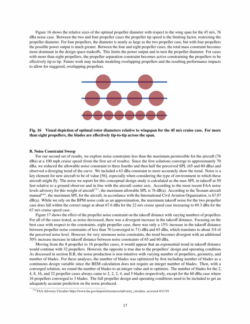
Figure 16 shows the relative sizes of the optimal propeller diameter with respect to the wing span for the 45 m/s, 76

dBa noise case. Between the two and four propeller cases the propeller tip speed is the limiting factor, restricting the

propeller diameter. For four propellers, the diameter is nearly as large as the two propeller case, but with four propellers

the possible power output is much greater. Between the four and eight propeller cases, the total mass constraint becomes

more dominant in the design space tradeoffs. This limits the power output and in turn the propeller diameter. For cases

with more than eight propellers, the propeller separation constraint becomes active constraining the propellers to be

effectively tip to tip. Future work may include modeling overlapping propellers and the resulting performance impacts

to allow for staggered, overlapping propellers.

Fig. 16 Visual depiction of optimal rotor diameters relative to wingspan for the 45 m/s cruise case. For more

than eight propellers, the blades are effectively tip-to-tip across the span.

B. Noise Constraint Sweep

For our second set of results, we explore noise constraints less than the maximum permissible for the aircraft (76

dBa) at a 100 mph cruise speed (from the first set of results). Since the first solutions converge to approximately 70

dBa, we reduced the allowable noise constraint to three fourths and then half the perceived SPL (65 and 60 dBa) and

observed a diverging trend of the curve. We included a 63 dBa constraint to more accurately show the trend. Noise is a

key element for new aircraft to be of value [56], especially when considering the type of environment in which these

aircraft might fly. The noise we report for this conceptual design study is calculated as the max SPL in takeoff at 50

feet relative to a ground observer and in line with the aircraft center axis. According to the most recent FAA noise

levels advisory for this weight of aircraft†††, the maximum allowable SPL is 76 dB(a). According to the Tecnam aircraft

manual∗∗∗, the maximum SPL for the aircraft, in accordance with the International Civil Aviation Organization, is 67.07

dB(a). While we rely on the BPM noise code as an approximation, the maximum takeoff noise for the two propeller

case does fall within the correct range at about 67.6 dBa for the 22 m/s cruise speed case increasing to 69.3 dBa for the

67 m/s cruise speed case.

Figure 17 shows the effect of the propeller noise constraint on the takeoff distance with varying numbers of propellers.

For all of the cases tested, as noise decreased, there was a divergent increase in the takeoff distance. Focusing on the

best case with respect to the constraints, eight propeller case, there was only a 15% increase in the takeoff distance

between propeller noise constraints of less than 76 (converged to 71) dBa and 65 dBa, which translates to about 3/4 of

the perceived noise level. However, for very strenuous noise constraints, the trend becomes divergent with an additional

50% increase increase in takeoff distance between noise constraints of 65 and 60 dBa.

Moving from the 8 propeller to 16 propeller cases, it would appear that an exponential trend in takeoff distance

would continue with 32 propellers. However, the opposite is true due to the propellers’ design and operating condition.

As discussed in section II.B, the noise production is non-intuitive with varying number of propellers, geometry, and

number of blades. For these analyses, the number of blades was optimized by first including number of blades as a

continuous design variable since the BEM calculation does not require an integer number of blades. Then, with a

converged solution, we round the number of blades to an integer value and re-optimize. The number of blades for the 2,

4, 8, 16, and 32 propeller cases always came to 2, 2, 2, 4, and 5 blades respectively, except for the 60 dBa case where

16 propellers converged to 3 blades. The full propeller design and operating conditions need to be included to get an

adequately accurate prediction on the noise produced.

†††FAA Advisory Circulars https://www.faa.gov/airports/resources/advisory_circulars, accessed 4/11/19

17

:

Fig. 17 Noise constraint effects on optimal takeoff distance with a fixed 45 m/s cruise speed constraint. De-

creasing the propeller noise constraint significantly increases takeoff distance. Less-than symbol indicates noise

constraint was not active

1. Noise Constrained Thrust

While the optimal propeller diameter and solidity remain relatively constant for a given number of propellers under

the varying noise constraint, the tip speed for more propellers decreases sharply. To achieve a similar SPL between

many high solidity propellers and a few lower solidity propellers, the tip speed of the greater number of propellers must

be significantly decreased. From the thrust coefficient equation T = CT ρn2D

4, with a relatively constant coefficient of

thrust CT , air density ρ, and diameter D, but changing rotation rate n, the generated thrust is decreased in an n2 manner

due to decreased tip speed. The effects of this can be seen in fig. 18 with the greater number of propellers experiencing

a much greater penalty on thrust to weight with decreasing noise constraint. However, even down to a noise constraint

of 63 dBa, the eight propeller takeoff distance is still below 100 m.

Fig. 18 Climb net thrust to weight with noise constraint effects, 45m/s cruise. Compare fig. 12a. Total climb

thrust in excess of 70% of the aircraft weight when the constraints on cruise speed are inactive.

18

2. Noise Constrained Lift Coefficient

With the decrease in available thrust due to the tip speed constraint, the propeller wake velocity is also decreased.

This decreases the dynamic pressure relative to a case with a higher blown velocity, and in turn, decreases the wing

lift coefficient. As seen in fig. 19 for the eight propeller case, the lift coefficient is decreased from 5.0 at the 76 dBa

constraint level to 3.5 at the 63 dBa constraint level. With decreased available thrust and decreased wing lift coefficient,

it takes longer to accelerate the same aircraft mass to a higher takeoff speed and still clear the 50 ft obstacle.

Fig. 19 Wing lift coefficient in the climb state. Compare fig. 13. Noise constraints significantly decrease the

ability of more propellers to produce excess dynamic pressure and in turn augmented lift coefficients.

VI. ConclusionsIn this study, we explored how continuously powered distributed electric propulsion on a Tecnam p2006t airframe

could be used as an immediate potential alternative to current urban air transport concepts. In this conceptual design

study, we found that a fully blown wing with 16 propellers could reduce the takeoff distance by over 50% when compared

to the optimal 2 propeller case. This resulted in a conceptual minimum takeoff distance of 20.5 meters to clear a 50 ft

(15.24 m) obstacle. We found that when decreasing the allowable noise to 60 dBa, the fully blown 8 propeller case

performed the best with a 43% reduction in takeoff distance compared to the optimal 2 propeller case at the same noise

constraint. The increase in takeoff distance due to noise constraints was divergent with relatively little effect until the

noise-performance tradeoffs become significant at levels below 65 dBa for all cases tested. For the 8 propeller case at

the 65 dBa constraint (70% of the perceived sound pressure level) there was only a 15% increase in the takeoff distance.

This case yielded a total conceptual takeoff distance of approximately 37 m. Further reducing allowable noise to a 60

dBa constraint (50% perceived noise reduction) resulted in an additional 2.4x increase in takeoff distance for the 8

propeller case.

We concluded that based on the results of this study, a distributed electric propulsion short takeoff and landing

fixed wing aircraft may be a candidate for the on demand mobility (ODM) urban air transport problem and warrants

future work in the area. The retrofit propulsion system in this study conceptually enabled the existing Tecnam p2006t to

achieve conceptual takeoff distances which would open thousands of potential options for urban air taxi runways. When

cruise speed and noise constraints are also included, the fully blown DEP system was still able to outperform the more

traditional 2 propeller system for the short range requirement modeled and still achieve a takeoff distance of less than

100 meters.

The main areas of future work critical to this study are in the design fidelity and the certification requirements. On

the design side, work could include more design freedom to completely change an aircraft configuration for a given

mission. Some possibilities include modeling propeller design that varies along the wingspan as well as including

propellers above or below the chord line to further influence the lift distribution and system efficiency. Optionally

powered and overlapping units, as well as including aircraft constraints on things such as brakes for landing, fuselage

19

structure for increased wing loading, stability, control, and full wing redesign could be included. The noise of the

electric motors, lifting surfaces, and control surfaces, could be added into the noise model. The second order motor

model including heat transfer could be included as well as a time-dependent battery model. Additionally, one might

model the landing portion of the flight including a final landing approach suggested by Patterson et al. [17], expand on

the landing as modeled by Courtin et al. [22], and model the optimal flight path similar to work by Hwang [7].

On the certification side, which is a critical component to the potential implementation of this concept, there is

significant work that would need to be done to access the safety, flight requirements, and potential changes to stall

regulations similar to those also suggested by Patterson [17] as well as required total field length when a balanced field

length is so short. Other areas may address safety requirements with multiple partially independent propulsion units,

urban gust and building wind factors, and required infrastructure.

VII. Code

The final code and data used to produce this work will be available on the BYU FLOW Lab website‡‡‡ following a

six month embargo period.

AcknowledgmentsThe authors gratefully acknowledge support from The Connectivity Lab at Facebook.

‡‡‡FLOW Lab http://flow.byu.edu

20

References[1] Gohardani, A. S., Doulgeris, G., and Singh, R., “Challenges of Future Aircraft Propulsion: A Review of Distributed Propulsion

Technology and its Potential Application for the All Electric Commercial Aircraft,” Progress in Aerospace Sciences, Vol. 47, No. 5,

2011, pp. 369–391. doi:10.1016/j.paerosci.2010.09.001, URL https://doi.org/10.1016%2Fj.paerosci.2010.09.001.

[2] Griffith, A., “Improvements Relating to Aircraft and Aircraft Engine Installations.” United Kingdom Patent, 720,394, 1954.

[3] Flittie, K., and Curtin, B., “Pathfinder solar-powered aircraft flight performance,” 23rd Atmospheric Flight Mechanics

Conference, AIAA, 1998. doi:10.2514/6.1998-4446, URL https://doi.org/10.2514%2F6.1998-4446.

[4] Yaros, S., Sexstone, M., Huebner, L., Lamar, J., McKinley., R., and Torres, A., “Synergistic Airframe–Propulsion Interactions

and Integrations: a White Paper Prepared by the 1996–1997 Langley Aeronautics Technical Committee,” Tech. Rep.

TM-1998-207644, NASA, Mar 1998.

[5] Noll, T. E., Ishmael, S. D., Henwood, B., Perez-Davis, M. E., Tiffany, G. C., Madura, J., Gaier, M., Brown, J. M., and

Wierzbanowski, T., “Technical Findings, Lessons Learned, and Recommendations Resulting from the Helios Prototype Vehicle

Mishap,” NASA Langley Research Center Hampton VA., 2007.

[6] Moore, M. D., “The Third Wave of Aeronautics: On-Demand Mobility,” SAE Technical Paper Series, SAE Transactions, 2006,

pp. 713–722. doi:10.4271/2006-01-2429, URL https://doi.org/10.4271%2F2006-01-2429.

[7] Hwang, J. T., and Ning, A., “Large-scale Multidisciplinary Optimization of an Electric Aircraft for On-Demand Mobility,”

2018 AIAA/ASCE/AHS/ASC Structures, Structural Dynamics, and Materials Conference, American Institute of Aeronautics and

Astronautics, 2018. doi:10.2514/6.2018-1384, URL https://doi.org/10.2514%2F6.2018-1384.

[8] Stoll, A. M., Bevirt, J., Moore, M. D., Fredericks, W. J., and Borer, N. K., “Drag Reduction Through Distributed Electric

Propulsion,” 14th AIAA Aviation Technology, Integration, and Operations Conference, AIAA, 2014. doi:10.2514/6.2014-2851,

URL https://doi.org/10.2514%2F6.2014-2851.

[9] Borer, N. K., Derlaga, J. M., Deere, K. A., Carter, M. B., Viken, S., Patterson, M. D., Litherland, B., and Stoll, A.,

“Comparison of Aero-Propulsive Performance Predictions for Distributed Propulsion Configurations,” 55th AIAA Aerospace

Sciences Meeting, American Institute of Aeronautics and Astronautics, 2017. doi:10.2514/6.2017-0209, URL https:

//doi.org/10.2514%2F6.2017-0209.

[10] Harish, A., Perron, C., Bavaro, D., Ahuja, J., Ozcan, M., Justin, C. Y., Briceno, S. I., German, B. J., and Mavris,

D., “Economics of Advanced Thin-Haul Concepts and Operations,” 16th AIAA Aviation Technology, Integration, and

Operations Conference, American Institute of Aeronautics and Astronautics, 2016. doi:10.2514/6.2016-3767, URL https:

//doi.org/10.2514%2F6.2016-3767.

[11] Patterson, M. D., and German, B., “Conceptual Design of Electric Aircraft with Distributed Propellers: Multidisciplinary

Analysis Needs and Aerodynamic Modeling Development,” 52nd Aerospace Sciences Meeting, American Institute of Aeronautics

and Astronautics, 2014. doi:10.2514/6.2014-0534, URL https://doi.org/10.2514%2F6.2014-0534.

[12] Deere, K. A., Viken, J. K., Viken, S., Carter, M. B., Wiese, M., and Farr, N., “Computational Analysis of a Wing Designed

for the X-57 Distributed Electric Propulsion Aircraft,” 35th AIAA Applied Aerodynamics Conference, American Institute of

Aeronautics and Astronautics, 2017. doi:10.2514/6.2017-3923, URL https://doi.org/10.2514%2F6.2017-3923.

[13] Dubois, A., van der Geest, M., Bevirt, J., Christie, R., Borer, N. K., and Clarke, S. C., “Design of an Electric Propulsion System

for SCEPTOR’s Outboard Nacelle,” 16th AIAA Aviation Technology, Integration, and Operations Conference, American Institute

of Aeronautics and Astronautics, 2016. doi:10.2514/6.2016-3925, URL https://doi.org/10.2514%2F6.2016-3925.

[14] Clarke, S., Redifer, M., Papathakis, K., Samuel, A., and Foster, T., “X-57 power and command system design,” 2017 IEEE

Transportation Electrification Conference and Expo (ITEC), IEEE, 2017, pp. 393–400. doi:10.1109/ITEC.2017.7993303, URL

https://doi.org/10.1109/ITEC.2017.7993303.

[15] Papathakis, K. V., Schnarr, O. C., Lavelle, T. M., Borer, N. K., Stoia, T., and Atreya, S., “Integration Concept for a

Hybrid-Electric Solid-Oxide Fuel Cell Power System into the X-57 “Maxwell”,” 2018 Aviation Technology, Integration,

and Operations Conference, American Institute of Aeronautics and Astronautics, 2018. doi:10.2514/6.2018-3359, URL

https://doi.org/10.2514/6.2018-3359.

[16] Falck, R. D., Chin, J., Schnulo, S. L., Burt, J. M., and Gray, J. S., “Trajectory Optimization of Electric Aircraft Subject to

Subsystem Thermal Constraints,” 18th AIAA/ISSMO Multidisciplinary Analysis and Optimization Conference, American Institute

of Aeronautics and Astronautics, 2017. doi:10.2514/6.2017-4002, URL https://doi.org/10.2514%2F6.2017-4002.

21

[17] Patterson, M. D., and Borer, N. K., “Approach Considerations in Aircraft with High-Lift Propeller Systems,” 17th AIAA

Aviation Technology, Integration, and Operations Conference, American Institute of Aeronautics and Astronautics, 2017.

doi:10.2514/6.2017-3782, URL https://doi.org/10.2514%2F6.2017-3782.

[18] Holmes, B. J., “A Vision and Opportunity for Transformation of On-Demand Air Mobility,” 16th AIAA Aviation Technology,

Integration, and Operations Conference, American Institute of Aeronautics and Astronautics, 2016. doi:10.2514/6.2016-3465,

URL https://doi.org/10.2514%2F6.2016-3465.

[19] Antcliff, K. R., Moore, M. D., and Goodrich, K. H., “Silicon Valley as an Early Adopter for On-Demand Civil VTOL Operations,”

16th AIAA Aviation Technology, Integration, and Operations Conference, American Institute of Aeronautics and Astronautics,

2016. doi:10.2514/6.2016-3466, URL https://doi.org/10.2514%2F6.2016-3466.

[20] Holmes, B. J., Durham, M. H., and Tarry, S. E., “Small Aircraft Transportation System Concept and Technologies,” Journal of

Aircraft, Vol. 41, No. 1, 2004, pp. 26–35. doi:10.2514/1.3257, URL https://doi.org/10.2514%2F1.3257.

[21] Moore, K. R., and Ning, A., “Distributed Electric Propulsion Effects on Existing Aircraft Through Multidisciplinary

Optimization,” 2018 AIAA/ASCE/AHS/ASC Structures, Structural Dynamics, and Materials Conference, American Institute of

Aeronautics and Astronautics, 2018. doi:10.2514/6.2018-1652, URL https://doi.org/10.2514%2F6.2018-1652.

[22] Courtin, C., Burton, M. J., Yu, A., Butler, P., Vascik, P. D., and Hansman, R. J., “Feasibility Study of Short Takeoff

and Landing Urban Air Mobility Vehicles using Geometric Programming,” 2018 Aviation Technology, Integration, and

Operations Conference, American Institute of Aeronautics and Astronautics, 2018. doi:10.2514/6.2018-4151, URL https:

//doi.org/10.2514%2F6.2018-4151.

[23] Ning, A., “A Simple Solution Method for the Blade Element Momentum Equations with Guaranteed Convergence,” Wind

Energy, Vol. 17, No. 9, 2014, pp. 1327–1345. doi:10.1002/we.1636, URL https://doi.org/10.1002%2Fwe.1636.

[24] “US standard atmosphere 1976,” Tech. Rep. NASA-TM-X-74335, NASA, 1976.

[25] Glauert, H., “Airplane Propellers. In: Aerodynamic Theory,” Springer, Berlin, Heidelberg, 1935, pp. 169–360. doi:

https://doi.org/10.1007/978-3-642-91487-4_3.

[26] Alvarez, E. J., and Ning, A., “Development of a Vortex Particle Code for the Modeling of Wake Interaction in Distributed

Propulsion,” 2018 Applied Aerodynamics Conference, American Institute of Aeronautics and Astronautics, 2018. doi:

10.2514/6.2018-3646, URL https://doi.org/10.2514%2F6.2018-3646.

[27] Veldhuis, L. L. M., “Propeller Wing Aerodynamic Interference,” Ph.D. thesis, Technical University of Delft, June 2005.

[28] Epema, H., “Wing Optimisation for Tractor Propeller Configurations,” Master’s thesis, Delft University of Technology, Jun

2017.

[29] Ning, S. A., “AirfoilPrep.py Documentation: Release 0.1.0,” Tech. rep., sep 2013. doi:10.2172/1260130, URL https:

//doi.org/10.2172%2F1260130.

[30] Du, Z., and Selig, M., “A 3-D Stall-Delay Model for Horizontal Axis Wind Turbine Performance Prediction,” 1998

ASME Wind Energy Symposium, American Institute of Aeronautics and Astronautics, 1998. doi:10.2514/6.1998-21, URL

https://doi.org/10.2514%2F6.1998-21.

[31] Eggers, A. J., Chaney, K., and Digumarthi, R., “An Assessment of Approximate Modeling of Aerodynamic Loads on the UAE

Rotor,” ASME 2003 Wind Energy Symposium, ASME, 2003. doi:10.2514/6.2003-868, URL https://doi.org/10.2514/6.

2003-868.

[32] Viterna, L. A., and Janetzke, D. C., “Theoretical and Experimental Power from Large Horizontal-Axis Wind Turbines,” Tech.

rep., Sep 1982. doi:10.2172/6763041, URL https://doi.org/10.2172%2F6763041.

[33] Tingey, E. B., and Ning, A., “Trading Off Sound Pressure Level and Average Power Production for Wind Farm Layout

Optimization,” Renewable Energy, Vol. 114, 2017, pp. 547–555. doi:10.1016/j.renene.2017.07.057, URL https://doi.org/

10.1016%2Fj.renene.2017.07.057.

[34] Brooks, T. F., and Marcolini, M. A., “Airfoil Tip Vortex Formation Noise,” AIAA Journal, Vol. 24, No. 2, 1986, pp. 246–252.

doi:10.2514/3.9252, URL https://doi.org/10.2514%2F3.9252.

[35] Brooks, T. F., Pope, D. S., and Marcolini, M. A., “Airfoil Self-Noise and Prediction,” Tech. Rep. 1218, NASA, July 1989.

22

[36] Ning, S. A., “pBEAM Documentation: Release 0.1.0,” Tech. rep., Sep 2013. doi:10.2172/1260133, URL https://doi.org/

10.2172%2F1260133.

[37] Kassapoglou, C., “Design and Analysis of Composite Structures: With Applications to Aerospace Structures,” John Wiley &

Sons, 2013, pp. 55–63. doi:10.1002/9781118536933.

[38] Tsai, S. W., and Wu, E. M., “A General Theory of Strength for Anisotropic Materials,” Journal of Composite Materials, Vol. 5,

No. 1, 1971, pp. 58–80. doi:10.1177/002199837100500106, URL https://doi.org/10.1177%2F002199837100500106.

[39] Tomblin, J., Sherraden, J., Seneviratne, W., and Raju, K., “Advanced General Aviation Transport Experiments. A–Basis and

B–Basis Design Allowables for Epoxy–Based Prepreg Toray T700GC-12K-31E/# 2510 Unidirectional Tape,” National Institute

for Aviation Research Wichita State University, Wichita, Kansas, 2002.

[40] Tomblin, J., Sherraden, J., Seneviratne, W., and Raju, K., “Advanced General Aviation Transport Experiments. ABasis and

BBasis Design Allowables for Epoxy Based Prepreg: TORAY T700SC-12K-50C/#2510 Plain Weave Fabric,” National Institute

for Aviation Research Wichita State University, Wichita, Kansas, 2002.

[41] Johnson, A., “Structural Component Design Techniques,” Handbook of Polymer Composites for Engineers, Elsevier, 1994, pp.

136–180. doi:10.1533/9781845698607.136, URL https://doi.org/10.1533%2F9781845698607.136.

[42] Lan, C. E., “A Quasi-Vortex-Lattice Method in Thin Wing Theory,” Journal of Aircraft, Vol. 11, No. 9, 1974, pp. 518–527.

doi:10.2514/3.60381, URL https://doi.org/10.2514%2F3.60381.

[43] Alba, C., Elham, A., German, B., and Veldhuis, L. L., “A Surrogate-Based Multi-Disciplinary Design Optimization Framework

Exploiting Wing-Propeller Interaction,” 18th AIAA/ISSMO Multidisciplinary Analysis and Optimization Conference, American

Institute of Aeronautics and Astronautics, 2017. doi:10.2514/6.2017-4329, URL https://doi.org/10.2514/6.2017-4329.

[44] Hunsaker, D., and Snyder, D., A Lifting-Line Approach to Estimating Propeller/Wing Interactions, American Institute of

Aeronautics and Astronautics, 2006. doi:10.2514/6.2006-3466, URL https://doi.org/10.2514/6.2006-3466.

[45] Veldhuis, L. L. M., “Review of Propeller-Wing Aerodynamic Interference,” International Congress of the Aeronautical Sciences,

2004.

[46] Abbott, I. H., and von Doenhoff, A. E., “Theory of Wing Sections: Including a Summary of Airfoil Data,” Courier Corporation,

2012, Chaps. High-Lift Devices, pp. 188–247.

[47] Drela, M., “First Order DC Electric Motor Model,” Tech. rep., MIT, Cambridge Massachusetts, Feb 2007.

[48] Mikhaylik, Y. V., Kovalev, I., Schock, R., Kumaresan, K., Xu, J., and Affinito, J., “High Energy Rechargeable Li-S

Cells for EV Application: Status, Remaining Problems and Solutions,” ECS, 2010. doi:10.1149/1.3414001, URL https:

//doi.org/10.1149%2F1.3414001.

[49] Anderson, J., Introduction to Flight, McGraw-Hill Higher Education, 2015, pp. 447–455,469–474.

[50] Anderson, “Aircraft Performance & Design,” Tata McGraw-Hill Education, 1999, pp. 265–267. doi:10.1036/0070019711.

[51] Mair, W. A., and Birdsall, D. L., “Take-off and Landing Performance,” Aircraft Performance, Cambridge University Press,

1992, pp. 119–161. doi:10.1017/cbo9780511607134.008, URL https://doi.org/10.1017%2Fcbo9780511607134.008.

[52] Kroo, I., “Propeller-Wing Integration for Minimum Induced Loss,” Journal of Aircraft, Vol. 23, No. 7, 1986, pp. 561–565.

doi:10.2514/3.45344, URL https://doi.org/10.2514%2F3.45344.

[53] Gill, P. E., Murray, W., and Saunders, M. A., “SNOPT: An SQP algorithm for largescale constrained optimization,” SIAM

Journal on Optimization, Vol. 12, No. 4, 2002, pp. 979–1006. doi:10.2307/20453604.

[54] Borer, N. K., Patterson, M. D., Viken, J. K., Moore, M. D., Bevirt, J., Stoll, A. M., and Gibson, A. R., “Design and Performance

of the NASA SCEPTOR Distributed Electric Propulsion Flight Demonstrator,” 16th AIAA Aviation Technology, Integration,

and Operations Conference, American Institute of Aeronautics and Astronautics, 2016. doi:10.2514/6.2016-3920, URL

https://doi.org/10.2514%2F6.2016-3920.

[55] Lunaas, C., “Category “A” operations for twin-engine helicopters,” Journal of Air Medical Transport, Vol. 10, No. 11,

1991, pp. 15 – 18. doi:https://doi.org/10.1016/S1046-9095(05)80504-5, URL http://www.sciencedirect.com/science/

article/pii/S1046909505805045.

[56] Moore, M. D., “Misconceptions of Electric Aircraft and their Emerging Aviation Markets,” 52nd Aerospace Sciences Meeting,

American Institute of Aeronautics and Astronautics, 2014. doi:10.2514/6.2014-0535, URL https://doi.org/10.2514%

2F6.2014-0535.

23