JIMS Round Up| JIMS corporate Interface, Top Ranked Management college in Delhi/NCR

SYSTEM SOFTWARE
BCA - 502


SYSTEM SOFTWARE
BCA - 502
This SIM has been prepared exclusively under the guidance of Punjab Technical
University (PTU) and reviewed by experts and approved by the concerned statutory
Board of Studies (BOS). It conforms to the syllabi and contents as approved by the
BOS of PTU.

Author: Sanjay Saxena
Copyright © Author, 2006
Reprint 2008, 2009, 2010
Reviewer
Dr. N. Ch. S.N. IyengarSenior Professor, School of Computing Sciences,VIT University, Vellore
Vikas® is the registered trademark of Vikas® Publishing House Pvt. Ltd.
VIKAS® PUBLISHING HOUSE PVT LTDE-28, Sector-8, Noida - 201301 (UP)Phone: 0120-4078900 • Fax: 0120-4078999
Regd. Office: 576, Masjid Road, Jangpura, New Delhi 110 014• Website: www.vikaspublishing.com • Email: [email protected]
All rights reserved. No part of this publication which is material protected by this copyright noticemay be reproduced or transmitted or utilized or stored in any form or by any means now known or
hereinafter invented, electronic, digital or mechanical, including photocopying, scanning, recording
or by any information storage or retrieval system, without prior written permission from the Publisher.
Information contained in this book has been published by VIKAS® Publishing House Pvt. Ltd. and hasbeen obtained by its Authors from sources believed to be reliable and are correct to the best of theirknowledge. However, the Publisher and its Authors shall in no event be liable for any errors, omissions
or damages arising out of use of this information and specifically disclaim any implied warranties or
merchantability or fitness for any particular use.

CAREER OPPORTUNITIES
Computer software engineers are projected to be one of the fastest growing occupationsin the next decade.
Computer applications software engineers analyse users' needs and design, construct,and maintain general computer applications software or specialized utility programs.
Computer system software engineers coordinate the construction and maintenance ofa company's computer systems and plan their future growth. System software engineerswork for companies that configure, implement, and install complete computer systems.Increasing emphasis on computer security suggests that software engineers withadvanced degrees that include system design will be sought after by software developers,government agencies, and consulting firms specializing in information assurance andsecurity.
As is the case with most occupations, advancement opportunities for computer softwareengineers increase with experience. Entry-level computer software engineers are likelyto test and verify ongoing designs. As they become more experienced, they may becomea project manager, manager of information systems, or chief information officer. Somecomputer software engineers with several years of experience or expertise find lucrativeopportunities working as system designers or independent consultants or starting theirown computer consulting firms.
The largest concentration of computer software engineers - almost 30 per cent - are incomputer system design and related services. Rapid employment growth in the computersystem design and related services industry, which employs the greatest number ofcomputer software engineers, should result in very good opportunities for those collegegraduates with at least a bachelor's degree in computer engineering or computer scienceand practical experience working with computers. Employers will continue to seekcomputer professionals with strong programming, system analysis, interpersonal andbusiness skills.
New growth areas will continue to arise from rapidly evolving technologies. Theincreasing uses of the Internet, the proliferation of Web sites, and mobile technologysuch as the Wireless Internet have created a demand for a wide variety of new products.As individuals and businesses rely more on hand-held computers and wirelessnetworks, it will be necessary to integrate current computer systems with this new,more mobile technology. Also, information security concerns have given rise to newsoftware needs. Concerns over "cyber security" should result in businesses andgovernment continuing to invest heavily in software that protects their networks andvital electronic infrastructure from attack. The expansion of this technology in the next10 years will lead to an increased need for computer engineers to design and developthe software and systems to run these new applications and integrate them into oldersystems.

PTU DEP SYLLABI-BOOK MAPPING TABLEBCA - 502 System Software
Section-IIntroduction to Software Processors: Elements of assembly languageprogramming; assembly scheme, single pass and two-pass assembler; generaldesign procedure of a two-pass assembler.
Section-IIMacros and Macro Processor: Macro definition, macro expansion, and featuresof macro facility, design of macro processor.
Overview of Compilers: Memory allocation, lexical analysis, syntax analysis,Intermediate code generation and optimization-local and global optimization,code generation.
Section-IIILoaders and Linkage Editors: Introduction to loading, linking and relocation,program linking, linkage editors, dynamic linking, bootstrap loader. Othersystem software: Operating System, DBMS, Functions and structure of TextEditor.
Unit 1: Introduction to SoftwareProcessors (Pages 3-19)
Unit 2: Macros and Macroprocessor(Pages 20-37);
Unit 3: Introduction to Compilers(Pages 38-49)
Unit 4: Loaders and Linkage Editor(Pages 50-68);
Unit 5: Other System Softwares(Pages 69-79)

CONTENTS
INTRODUCTION 1
UNIT 1 INTRODUCTION TO SOFTWARE PROCESSORS 3–191.0 Introduction; 1.1 Unit Objectives;1.2 Introduction to Software Processors;1.2.1 Complex Instruction Set Computer (CISC); 1.2.2 Reduced Instruction Set Computer (RISC);1.2.3 Hybrid Processors; 1.2.4 Special Purpose Processors1.3 Elements of Assembly Language Programming;1.3.1 Instructions; 1.3.2 Integer expressions; 1.3.3 Reserved Words and Identifiers; 1.3.4 Directives1.4 Assembly Scheme;1.5 Single-Pass and Two-Pass Assembler;1.5.1 Working of an Assembler; 1.5.2 Single-Pass Assembler; 1.5.3 Two-Pass Assembler1.6 General Design Procedure of a Two-Pass Assembler; 1.7 Summary;1.8 Answers to ‘Check your Progress’; 1.9 Exercises and Questions; 1.10 Further Reading
UNIT 2 MACROS AND MACROPROCESSOR 20–372.0 Introduction; 2.1 Unit Objectives; 2.2 Macro Definition;2.3 Macro Expansion; 2.4 Nested Macro Calls;2.5 Features of Macro Facility;2.5.1 Macro Instruction Arguments; 2.5.2 Conditional Macro Expansion; 2.5.3 Macro Instructions Defining Macros2.6 Design of a Macro Pre-processor;2.6.1 Implementation of Two-Pass Algorithm; 2.6.2 Implementation of Single-Pass Algorithm2.7 Summary; 2.8 Answers to ‘Check your Progress’;2.9 Exercises and Questions; 2.10 Further Reading
UNIT 3 INTRODUCTION TO COMPILERS 38–493.0 Introduction; 3.1 Unit Objectives;3.2 Overview of Compilers;3.2.1 Cross Compiler; 3.2.2 One-Pass or Multi-pass Compiler; 3.2.3 Source-to-source Compiler;3.2.4 Stage Compiler; 3.2.5 Just-in-time Compiler3.3 Structure of Compiler;3.3.1 Scanner; 3.3.2 Parser; 3.3.3 Symbol Tables and Error Handler;3.3.4 Contextual Checkers; 3.3.5 Intermediate Code Generator;3.3.6 Code Optimizer; 3.3.7 Code Generator; 3.3.8 Peep Hole Optimizer3.4 Example of a Compiler;3.5 Phases of a Compiler;3.5.1 Lexical Analysis Phase; 3.5.2 Syntax Analysis Phase;3.5.3 Intermediate Code Generation Phase; 3.5.4 Native Code Generation Phase; 3.5.5 Optimization Phase3.6 Summary; 3.7 Answers to ‘Check your Progress’;3.8 Exercises and Questions; 3.9 Further Reading
UNIT 4 LOADERS AND LINKAGE EDITORS 50–684.0 Introduction; 4.1 Unit Objectives;4.2 Overview of Loaders and Linkers;4.2.1 Object Modules; 4.2.2 Binary Programs4.3 Loaders;4.3.1 Compile and Go Loader; 4.3.2 Absolute Loader;4.3.3 Relocating Loaders; 4.3.4 Direct-Linking Loaders

4.4 Linkage Editor;4.4.1 Program Relocation; 4.4.2 Program Linking4.5 Design of a Linker;4.5.1 First Pass; 4.5.2 Second Pass4.6 Dynamic Linking; 4.7 Bootstrap Loader; 4.8 Summary;4.9 Answers to ‘Check your Progress’; 4.10 Exercises and Questions; 4.11 Further Reading
UNIT 5 OTHER SYSTEM SOFTWARES 69-795.0 Introduction; 5.1 Unit Objectives; 5.2 Operating System;5.3 Types of Operating Systems;5.3.1 Multiprocessing Operating System; 5.3.2 Multitasking; 5.3.3 Multi-user;5.3.4 Multithreading; 5.3.5 Real-time Operating System5.4 Functions of Operating System;5.4.1 Process Management; 5.4.2 Memory and Storage Management; 5.4.3 Protection and Security5.5 DataBase Management System (DBMS);5.5.1 Data; 5.5.2 Hardware; 5.5.3 Software; 5.5.4 End Users5.6 Entities and Relationships; 5.7 Functions and Structure of Text Editor; 5.8 Summary;5.9 Answers to ‘Check your Progress’; 5.10 Exercises and Questions; 5.11 Further Reading

Punjab Technical University 1
Introduction
NOTES
Self-Instructional Material
INTRODUCTION System Software is necessarily an important concept in order to communicate with your computer system. It is required to understand the architecture and the interface used in a system so that it becomes easy for a programmer to administer the instructions provided. In this book, we will discuss the concepts that include the use and implementation of assemblers, macros, loaders, compilers and operating systems. We have made an attempt to present all these components in detail with the help of examples.
How This Book is Organized This book is divided into five units:
Unit 1 Introduction to Software Processors discusses the software processors. You will get to know about the different elements of an assembly language programming. It, thereafter, describes the general design procedure of a two-pass assembler. The next section in this chapter discusses about the software tools in which the concept and design of text editor is mentioned.
Unit 2 Macros and Microprocessors explains the concept of defining and expanding macros. Followed by this, it describes various features of macro facility. It also focuses your attention on different types of interpreters and loaders.
Unit 3 Compilers helps understand the aspects of compilation and different phases of a compiler. In addition, you will learn about the important concepts related to linkers such as relocating and linking.
Unit 4 Loaders and linkers discusses about the loaders and linkers that helps in the creation of a program. Linkers connect the object module with the binary program. The loaders help converting the source program into the object program.
Unit 5 Other System Software discusses about the operating system. It also describes the various types of operating systems such as multiprocessing and multitasking. The functions of operating system are also discussed in detail. In addition, this unit also gives an overview of database management system.

2 Self-Instructional Material
Linux Administration
NOTES

Punjab Technical University 3
Introduction to Software Process
NOTES
Self-Instructional Material
UNIT 1 INTRODUCTION TO SOFTWARE PROCESSORS
Structure 1.0 Introduction 1.1 Unit Objectives 1.2 Introduction to Software Processors
1.2.1 Complex Instruction Set Computer (CISC); 1.2.2 Reduced Instruction Set Computer (RISC); 1.2.3 Hybrid Processors; 1.2.4 Special Purpose Processors
1.3 Elements of Assembly Language Programming 1.3.1 Instructions; 1.3.2 Integer expressions; 1.3.3 Reserved Words and Identifiers; 1.3.4 Directives
1.4 Assembly Scheme 1.5 Single-Pass and Two-Pass Assembler
1.5.1 Working of an Assembler; 1.5.2 Single-Pass Assembler; 1.5.3 Two-Pass Assembler
1.6 General Design Procedure of a Two-Pass Assembler 1.7 Summary 1.8 Answers to ‘Check your Progress’ 1.9 Exercises and Questions 1.10 Further Reading 1.0 INTRODUCTION
A software processor is a device such as CPU and I/O channel that operates on the information stored in the memory of a computer. These devices use the information that you store in the memory of a computer for performing various tasks, such as input of character and displaying an output on the computer screen. Software such as traffic controller and scheduler helps a software processor to control running processes in a computer. Computers use assembly language to execute instructions given to the computer. Assembly language uses the concept of single-pass and two pass for executing instructions given to the computer, such assemblers are known as single-pass assembler and two-pass assemblers. 1.1 UNIT OBJECTIVES
• Discussing the concept that a software processor uses • Introducing the elements of an assembly language • Describing assembly scheme • Discussing single and two-pass assembler • Describing general design procedure of a two-pass assembler

4 Punjab Technical University
System Software
NOTES
Self-Instructional Material
1.2 INTRODUCTION TO SOFTWARE PROCESSORS
A software processor is a device such as CPU and I/O channel that processes the information stored in the memory of a system to generate an output. Processors can broadly be divided into following categories:
• Complex Instruction Set Computers (CISC) • Reduced Instruction Set Computers (RISC) • Hybrid processors, and • Special purpose processors
1.2.1 Complex Instruction Set Computer (CISC) CISC performs most of the computer work in the shortest time. It consists of a large instruction set with hardware support for a wide variety of operations. CISC processors are used in scientific, engineering and mathematical operations with hand coded assembly language. You can also use CISC processors in some of the business applications where hand-coded assembly languages are used. The CDC 6600, Motorola 68000 family and AMD x86 CPUs are examples of CISC processors. Some advantages of the CISC design are as follows:
• A new CISC processor design contains the instruction set of the old processors and the new changes are added to the new design of the processor. Therefore, you do not need to re-write code for every new design cycle of the CISC processor.
• For a CISC processor design, fewer instructions are needed to implement a particular computing task, which lead to lower memory use for program storage and takes less time to fetch instruction from the processor of the computer.
• CISC makes the language of the computer more like assembly language that helps in less compilation work.
Some disadvantages of the CISC design philosophy are as follows: • The first advantage listed above can also be viewed as a disadvantage. That
is, the incorporation of older instruction sets into new generations of processors tend to force growing complexity of CISC processors.
• Each CISC command must be translated by the processor into tens or even hundreds of lines of microcode, it tends to run slower than an equivalent series of simpler commands that do not require so much translation, as translation requires time.
• CISC machine builds complexity in the processor, where its various commands must be translated into microcode for actual execution of the instructions, the design of CISC hardware is more difficult and CISC design cycle to add new instructions to the CISC processor is correspondingly long.
1.2.2 Reduced Instruction Set Computer (RISC) RISC consists of a small, compact instruction set that you use for executing instructions of a program. In most business applications and in programs created by compilers from high-level language source, RISC processors usually perform most work in the shortest time.

Punjab Technical University 5
Introduction to Software Process
NOTES
Self-Instructional Material
Examples of RISC processors are the AVR, PIC, ARM, DEC Alpha, PA-RISC, SPARC, MIPS and Power Architecture.
Some advantages of the RISC processor are as follows: • A new microprocessor can be developed and tested more quickly to reduce
the complexity of the RISC processor. • Operating system and application programmers, who use the microprocessor
instructions, will find it easier to develop code with a smaller instruction set. • The simplicity of RISC allows more freedom to select the usage of memory
space on a microprocessor, which helps store more instructions in the computer.
• Higher level language compilers produce more efficient code than low-level language compilers because high-level language compilers always tend to use the smaller set of instructions to be found in a RISC computer.
RISC processors provide following advantages over CISC processors: • RISC processors allow more room for performance-enhancing features, such
as cache memory, memory management functions and floating-point hardware that reduces execution time.
• RISC processors reduces development time, the simple RISC-based processor requires less processor designing and applications programming effort, and offers lower manufacturing costs.
• RISC processors include instruction decode logic, while CISC processors require large microcode ROMs to execute an instruction.
• RISC processors executes instruction in single clock cycle, while CISC processors require multiple clock cycles for executing an instruction.
1.2.3 Hybrid Processors Hybrid processor is a combination of CISC and RISC processors. Most CISC processors are based on hybrid CISC-RISC architecture. Hybrid processor designs use a decoder to convert CISC instructions into RISC instructions before execution of the instruction.
Examples of hybrid processor designs include the Pentium and Athlon family of processors. These processors are compatible with software written for their CISC predecessors and also perform competitively against processors based on RISC designs. However, CISC-RISC hybrid processors consume a lot of power and are not used for mobile and embedded applications.
1.2.4 Special Purpose Processors Special purpose processors are optimised to perform specific functions, such as executing digital signals. Digital signal processors and various kinds of co-processors are the most common kind of special purpose processors. 1.3 ELEMENTS OF ASSEMBLY LANGUAGE
PROGRAMMING
Assembly language is the most basic programming language available to any processor. Assembly language allows a programmer to work with operations that you can implement directly on the CPU for executing programs. An assembly language

6 Punjab Technical University
System Software
NOTES
Self-Instructional Material
source code file consists of collection of statements that helps the assembler to run the programs. These statements in assembly language include:
• Instructions: An instruction refers to the statement that is translated by an assembler into one or more bytes of machine code that executes at run time.
• Directives: A directive is responsible for instructing an assembler to take some action. The performed action does not have any effect on the object code. Such an action does not result in machine instructions.
• Macros: A macro is a shorthand notation for a sequence of statements. These statements can be instructions, directives or even macros. An assembler expands a macro and returns a sequence of statements already specified in the macro definition.
The basic building block of an assembly language program includes characters, identifiers, labels, constants and assembly language counter. Following are the basic elements of assembly programming language:
• Instructions • Integer expressions • Reserved words and identifiers • Directives
1.3.1 Instructions Instructions are assembled to machine code by assembler and executed at run-time by the CPU. Consider the following example of instruction used in assembly language:
No operands stc ; set Carry flag One operand inc eax ; register inc myByte ; memory Two operands add ebx,ecx ; register, register sub myByte,30 ; memory, constant add eax,35 * 15 ; register, constant-expression
The example shows that an instruction includes following parts: • Labels • Operands • Comments
1.3.1.1 Labels There is not much difference between an identifier and a label. A label is written as an identifier immediately followed by a colon (:). A label represents the current value of the current location counter that holds the current location of the instruction. You can use a label in assembler instruction as an operand. A label consists of a digit between 0 and 9 and must be followed by a colon. Local numeric labels allow compilers and programmers to use label names temporarily. The labels that have been created by you can be reused number of times throughout the program for representing the current value of the current location counter. The following example shows a label x that contains a value 20.
x: .word 20!int x = 20;

Punjab Technical University 7
Introduction to Software Process
NOTES
Self-Instructional Material
1.3.1.2 Operands You can use various operands in assembly language programming that help initialise data and store data. Operands may be of following types:
• constant (immediate value) • constant expression • memory (data label) • registers
Constants: There are four different types of constants such as numeric, character, string and floating-point, which helps store data. A numeric constant also starts with a digit and can be a decimal, hexadecimal or octal. The rules for a numeric constant are as follows:
• Decimal constants contain digits between 0 to 9 only. • Hexadecimal constants start with 0x (or 0X), followed decimal digits by
between one to eight or hexadecimal digits (0 to 9, a to f and A to F). • Octal constants start with 0 and are followed by one to eleven octal digits (0
to 7). Values that do not fit in 32 bits are bignums.
Constant Expression: A single character constant consists of a single quotation mark (‘) followed by an ASCII character. It can be an alphanumeric character, i.e., from A to Z or from a to z or from 0 to 9. The characters may also include other printable ASCII characters that include #, $, :, ., +, -, *, / and |. Additionally, the non-printable characters, which are ASCII characters such as space, tab, return and new line. Following example uses special character constants for creating a program using assembly language programming.
Enclose character in single or double quotes 'A', "b" ASCII character = 1 byte Enclose strings in single or double quotes "ABC" 'abc' Each character occupies a single byte Embedded quotes: 'Assembly "Language" Program'
Memory: The basic unit of memory is a byte that comprises of eight bits of information. Table 1.1 lists some other units of memory.
Table 1.1: Units of Memory
Unit of memory Bytes Equivalent bits
Byte 1 8
Halfword 2 16
Word 4 32
Doubleword 8 64

8 Punjab Technical University
System Software
NOTES
Self-Instructional Material
Registers: The registers are used mainly for storing various arithmetic and logical operations. There are 16 general-purpose registers in a processor and each consists of 32 bits of memory. In addition, there are 4 floating-point registers, each consisting of 64 bits of memory. The general-purpose registers are sometimes used as base registers also. For example, the instruction A 1,16(4, 10) interprets an add instruction. This instruction depicts a number that is to be added to the contents of register 1.
1.3.1.3 Comments A comment explains the program’s purpose and are of two types: single-line and multiple-line comments. Single-line comments begin with semicolon (;) and multi-line comments begin with COMMENT directive, and a programmer-chosen character ends with the same programmer-chosen character.
1.3.2 Integer Expressions An integer expression contains various constants and operators such as + and *. Table 1.2 lists various operators of integer expression and their precedence order that allow you to evaluate an expression.
Table 1.2: The Operators and Their Precedence Order
Operator Name Precedence Order
( ) Parenthesis 1
+, - Unary plus, minus 2
*, / Multiply, divide 3
MOD Modulus 4
+, - Add, subtract 5
1.3.3 Reserved Words and Identifiers Reserved words can be instruction mnemonics, directives, type attributes, operators and predefined symbols that are predefined in the language. The reserved words used in assembly language include following general categories of words:
• Operands and Symbols (MEMORY, FLAT, BYTE, DWORD, etc.) • Predefined Symbols (@code, @date, @time, @model, etc.) • Registers (eax, esp, ah, al, etc.) • Operators and Directives (.code, .data, etc.) • Processor Instructions (add, mov, call, etc.), and • Instruction Prefixes (LOCK, REP, etc.).
An assembly language program also includes identifiers. An identifier is also known as a symbol, which is used as a label for an assembler statement. It can also be used as a location tag for storing data. The symbolic name of a constant can also be determined by using identifiers. The rules that should be considered for identifiers are:
• An identifier should consist of a sequence of alphanumeric characters.

Punjab Technical University 9
Introduction to Software Process
NOTES
Self-Instructional Material
• The first character of an identifier must not be a numeric value. First character of an identifier must be a letter, like _, @ or $.
• An identifier can be of any length and all the characters of an identifier are significant.
• An identifier is case-sensitive. • Reserved words cannot be used as identifiers.
1.3.4 Directives Directives are the commands that are recognised and acted upon by the assembler. Directives are used for various purposes such as to declare code, data areas, select memory model and declare procedures. Directives are not case-sensitive and different assemblers can have different directives. Each group of variable declaration should be preceded by a data directive. Each group of assembly language instructions should be preceded by a text directive. The model directive tells the assembler to generate code that will run in protected mode and in 32-bit mode. The end directive marks the end of the program. The data and code directives mark the beginning of the data and code segments. The data is a read and write segment, and code is a read-only segment.
Example: Following example defines directives to allocate space for three variables, x, y and z. You should initialise these variables with decimal 20, hexadecimal 3fcc and decimal 41, respectively.
.data ! start a group of variable declarations x: .word 20 ! int x = 20; y: .word 0x3fcc ! int y = 0x3fcc; z: .word 41 ! int z = 41;
Example of an assembly program
You need to follow a syntax for creating a program in assembly language. Each assembly language statement has the following general form:
label operation operand(s) ; comments
Consider the following assembly program to add and subtract two 32-bit integers values.
TITLE Add and Subtract (AddSub.asm) ; This program adds and subtracts 32-bit integers. INCLUDE Irvine32.inc .code main PROC mov eax,10000h ; EAX = 10000h add eax,40000h ; EAX = 50000h sub eax,20000h ; EAX = 30000h call DumpRegs ; display registers exit main ENDP END main
1.4 ASSEMBLY SCHEME Once you have come across the elements of assembly language, you will know how to communicate with the computer that uses assembly language. The scheme followed in the assembly language is considered as a largely machine-dependent

10 Punjab Technical University
System Software
NOTES
Self-Instructional Material
scheme used by the programmers. The assembly language is preferred by programmers as it is easy to read and uses symbolic addresses.
The assembly scheme can be structured with the help of the following components: • USING: This is a pseudo-op, which is responsible for addressing registers.
Since, no special registers are maintained for this purpose, a programmer should inform an assembler that which register(s) to use and also how to use these registers. This pseudo-op decides which of the general registers are to be used as a base register and what should be the contents of the register.
• BALR: This is an instruction which informs an assembler to load a register with the next address. This instruction branch the address in the second field. It is important to note that in case the second operand is 0 in the BALR instruction, the execution starts proceeding with the next instruction. The major difference between the BALR and the USING components is that the BALR instruction loads a base register, whereas the USING pseudo-op does not load a register in the memory, rather it informs the assembler about the contents of the base register. If the register does not contain the address that is specified by the USING component, it results in a program error.
• START: This pseudo-op informs an assembler about the beginning of a program. It also allows a user to give a name to the program.
• END: This pseudo-op informs an assembler that the last address of a program has been reached.
• BR X: This is the instruction that branches to the location that has its address in general register X.
The assembly scheme can also contain addresses in the operand fields of an instruction. Figure 1.1 shows the implementation of assembly scheme:
Figure 1.1: The Implementation of Assembly Scheme
In the example, ASSEMBLY is the name of the program. The next instruction BALR 10,0 in the program sets register 10 to the address of the next instruction, as the second operation in the instruction is 0. Next comes USING BEGIN+2,10, the pseudo-op in this instruction is indicating to the assembler that register 10 as a base register and also that the content of the register 10 is the address of the next instruction. SR 4,4 clears register 4 and sets index to 0. The next instruction L 3, NINE loads the number 9 into register 3. The instruction L 2,DATA (8) loads data (index) into register 2. Next comes A 2, FORTYFIVE, which adds 45 to register 2.

Punjab Technical University 11
Introduction to Software Process
NOTES
Self-Instructional Material
Similarly, the next two instructions store the updated value of data (index) and 8 is added to register 8.
The next instruction BCT 3,LOOP will decrement register 3 by 1. In case, if the result generated by this instruction comes to non-zero, then it will branch back to the LOOP instruction. The instruction BR 14 would branch back to a caller that has called the LOOP instruction. The next three instructions contain DC pseudo-op, which indicates that these are the constants in a program. The next instruction is also a DC pseudo-op, which indicates the words that are to be processed in a program. The last instruction is the END instruction, which informs the assembler that the last card of the program has been reached. An assembly scheme provides advantages such as readability and easy understanding of the instructions. The primary disadvantage of an assembly scheme is that it uses an assembler to translate a source program into object code. 1.5 SINGLE-PASS AND TWO-PASS ASSEMBLER
An assembler is a program that is responsible for generating machine code instructions from a source code program. Source code programs are written in assembly languages and an assembler converts the written assembly language source program to a format that can be executed on a processor. Each machine code instruction is replaced by a mnemonic, an abbreviation that represents the actual information. An assembler is responsible for translating the programs written in the mnemonic assembler language into executable form. These mnemonics are frequently used in assembly programming as they reduce the chances of making an error.
Following are the features of an assembler: 1. It allows a programmer to use mnemonics while writing source code
programs. 2. It provides variables that are represented by symbolic names and not as
memory locations. 3. It allows error-checking procedure. 4. It allows making the changes and incorporating them with a reassembly. 5. It provides a symbolic code that is easy to read and follow.
An assembler can be a single-pass assembler or a two-pass assembler.
1.5.1 Working of an Assembler The essential task of an assembler is to convert symbolic text into binary values that are loaded into successive bytes of memory. There are three major components to this task.
1. Allocating and initialising storage, 2. Conversion of mnemonics to binary instructions, and 3. Resolving addresses using single or two-pass assembler.
An assembler scans through a file maintaining a set of “location pointers” for next available byte of each segment (.data, .text, .kdata and .ktext).

12 Punjab Technical University
System Software
NOTES
Self-Instructional Material
1.5.1.1 Allocating and Initialising Storage Assembler directives handle the memory allocation and initialise the storage. Consider the following assembly language program to understand the working of an assembler:
.data x: .word 40 msg: .asciiz “Hello, World” .align 2 array: .space 40 fun: .word 0xdeadbeef
The example consists of x, msg, array and fun labels and when an assembler encounters label declarations while scanning a source file, it creates a SYMBOL table entry to keep track of its location. Table 1.3 lists the SYMBOL table for different labels in the program:
Table 1.3: The Symbol Table
Symbol Segment Location Pointer Offset
X data 0
msg data 4
array data 20
fun data 60
1.5.1.2 Encoding Mnemonics Mnemonics generate binary encoded instructions; unresolved addresses are set to 0 in the location-offset pointer and set to unknown in the symbol table. An assembler also computes the offsets to branch targets such as loading a register. Table 1.4 lists the updated symbols after encoding the mnemonics:
Table 1.4: The Updated Symbol Table
Symbol Segment Location Pointer Offset
X data 0
Msg data 4
Array data 20
Fun data 60
Main text 0
Bitrev ? ?
Punjab Technical University 13
Introduction to Software Process
NOTES
Self-Instructional Material
1.5.1.3 Resolving Addresses You can also resolve addresses that are stored in memory. Resolving of address can be done using single-pass and two-pass assembler.
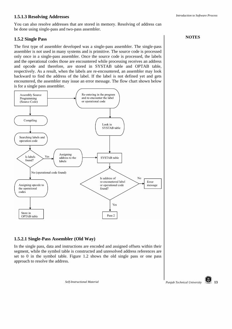
1.5.2 Single Pass The first type of assembler developed was a single-pass assembler. The single-pass assembler is not used in many systems and is primitive. The source code is processed only once in a single-pass assembler. Once the source code is processed, the labels and the operational codes those are encountered while processing receives an address and opcode and therefore, are stored in SYSTAB table and OPTAB table, respectively. As a result, when the labels are re-encountered, an assembler may look backward to find the address of the label. If the label is not defined yet and gets encountered, the assembler may issue an error message. The flow chart shown below is for a single pass assembler.
1.5.2.1 Single-Pass Assembler (Old Way) In the single pass, data and instructions are encoded and assigned offsets within their segment, while the symbol table is constructed and unresolved address references are set to 0 in the symbol table. Figure 1.2 shows the old single pass or one pass approach to resolve the address.

14 Punjab Technical University
System Software
NOTES
Self-Instructional Material
Figure 1.2: The Old Single-Pass Assembler Approach
1.5.2.2 Single-Pass Assembler (Modern Way) Modern assemblers keep more information in their symbol table, which allows them to resolve addresses in a single pass. Modern single-pass assemblers maintains two types of addresses as:
• Known addresses (backward references) are immediately resolved. • Unknown addresses (forward references) are “back-filled” once they are
resolved.
Figure 1.3 shows the symbol table after single-pass through the assembler in the modern way:
Figure 1.3: The Symbol Table After Single-Pass (Modern Way)
1.5.3 Two-Pass Assembler In a two-pass assembler, the source code is passed twice through an assembler. The first pass in a two-pass assembler is specifically for the purpose of assigning an address to all labels. Once all the labels get stored in a table with the appropriate addresses, the second pass is processed to translate the source code into machine code. After the second pass, the assembler generates the object program, assembly listing and output information for the linker to link the program. This is the most

Punjab Technical University 15
Introduction to Software Process
NOTES
Self-Instructional Material
popular type of assembler currently in use. The flow chart shown below is for a two-pass assembler.
Figure 1.4 shows the two-pass or double-pass assembler approach to resolve an address.
Figure 1.4: The Two-Pass Assembler Approach

16 Punjab Technical University
System Software
NOTES
Self-Instructional Material
1.6 GENERAL DESIGN PROCEDURE OF
A TWO-PASS ASSEMBLER
You need to follow a procedure that allows you to design a two-pass assembler. The general design procedure of an assembler involves the following six steps:
1. Specification of the problem
2. Specification of the data structures
3. Defining the format of data structures
4. Specifying the algorithm
5. Looking for modularity that ensures the capability of a program to be subdivided into independent programming units, and
6. Repeating step 1 to 5 on modules for accuracy and checking errors.
The operation of a two-pass assembler can be explained with the help of the following functions that are performed by an assembler while translating a program:
• It replaces symbolic addresses with numeric addresses. • It replaces symbolic operation codes with machine operation codes. • It reserves storage for instructions and data. • It translates constants into machine representation.
A two-pass assembler includes two passes, Pass1 and Pass 2. Therefore, it is named as two-pass assembler. In Pass 1 of the two-pass assembler, the assembler reads the assembly source program. Each instruction in the program is processed and is then translated to the generator. These translations are accumulated in appropriate tables, which help fetch a stored value. In addition to this, an intermediate form of each statement is generated. Once these translations have been made, Pass 2 starts its operation.
Pass 2 examines each statement that has been saved in the file containing the intermediate program. Each statement in this file searches for the translations and then assembles these translations into the machine language program. The primary aim of the first pass of a two-pass assembler is to draw up a symbol table. Once Pass 1 has been completed, all necessary information on each user-defined identifier should have been recorded in this table. A Pass 2 over the program then allows full assembly to take place quite easily. Refer to the symbol table whenever it is necessary to determine an address for a named label, or the value of a named constant. The first pass can also perform some error checking. Figure 1.5 shows the steps followed by a two-pass assembler:
Figure 1.5: The Functioning of a Two-Pass Assembler
Check Your Progress 1. An assembler is a program
that generates machine code instructions from a source code program. A. True B. False
2. The ……………pseudo-op informs the assembler that the last card of the program has been reached.
3. 1 word = ……………bits.
Punjab Technical University 17
Introduction to Software Process
NOTES
Self-Instructional Material
The table stores the translations that are made to the program. The table also includes operation table and symbol table. The operation table is denoted as OPTAB. The OPTAB table contains:
• Content: mnemonic, machine code (instruction format, length), etc. • Characteristic: static table, and • Implementation: array or hash table, easy for search.
An assembler designer is responsible for creating OPTAB table. Once the table is created, an assembler can use the tables contained within OPTAB, known as sub-tables. These sub-tables include mnemonics and their translations. The introduction of mnemonics for each machine instruction is subsequently gets translated into the machine language for the convenience of the programmers. There are four different types of mnemonics in an assembly language:
1. Machine operations such as ADD, SUB, DIV, etc. 2. Pseudo-operations or directives: Pseudo-ops are the data definitions. 3. Macro-operation definitions. 4. Macro-operation call, which includes calls such as PUSH and LOAD.
Another type of tables used in the two-pass assembler is the symbol table. The symbol table is denoted by SYMTAB. The SYMTAB table contains:
• Content: label name, value, flag, (type, length), etc. • Characteristic: dynamic table (insert, delete, search), and • Implementation: hash table, non-random keys, hashing function.
This table stores the symbols that are user-defined in the assembly program. These symbols may be identifiers, constants or labels. Another specification for symbol tables is that these tables are dynamic and you cannot predict the length of the symbol table. The implementation of SYMTAB includes arrays, linked lists and a hash table.
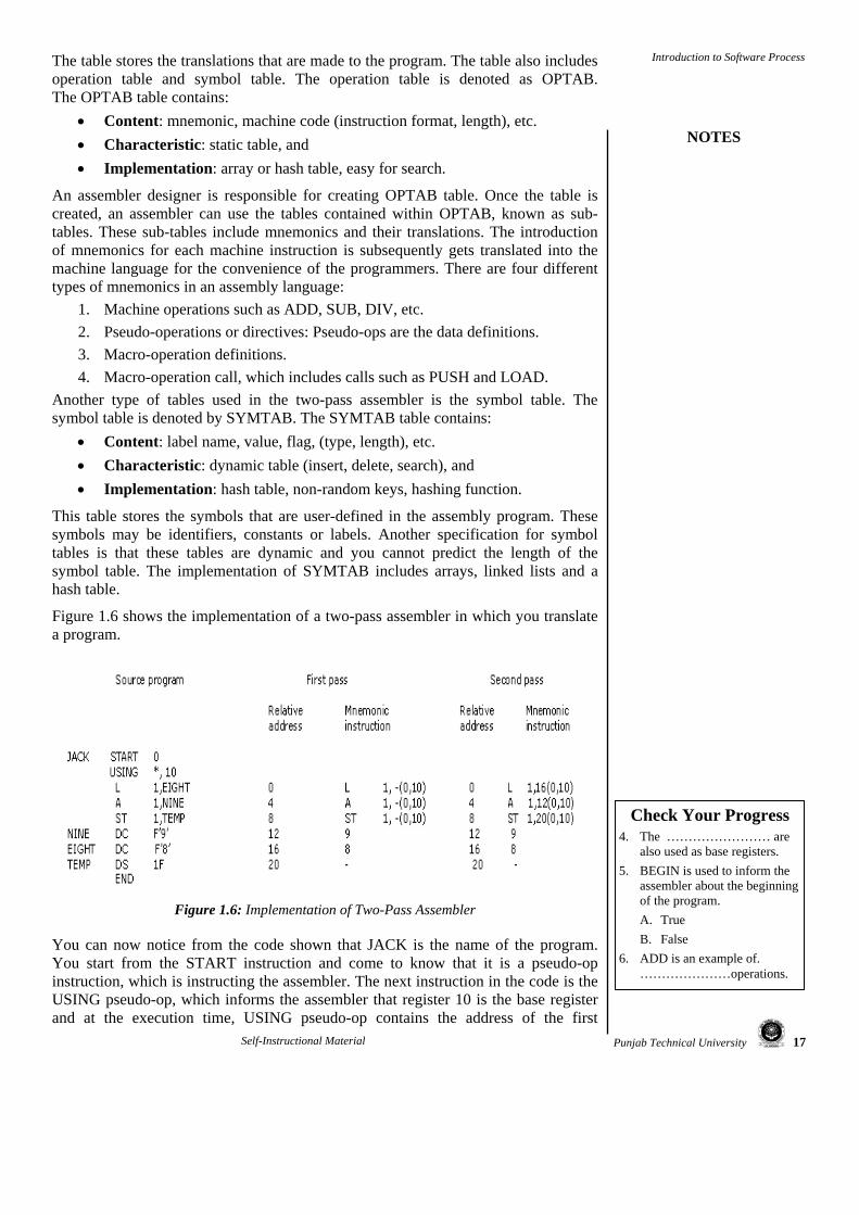
Figure 1.6 shows the implementation of a two-pass assembler in which you translate a program.
Figure 1.6: Implementation of Two-Pass Assembler
You can now notice from the code shown that JACK is the name of the program. You start from the START instruction and come to know that it is a pseudo-op instruction, which is instructing the assembler. The next instruction in the code is the USING pseudo-op, which informs the assembler that register 10 is the base register and at the execution time, USING pseudo-op contains the address of the first
Check Your Progress 4. The …………………… are
also used as base registers. 5. BEGIN is used to inform the
assembler about the beginning of the program. A. True B. False
6. ADD is an example of. …………………operations.

18 Punjab Technical University
System Software
NOTES
Self-Instructional Material
instruction of the program. Next in the code is the load instruction: L 1,EIGHT and to execute this instruction, the assembler needs to have the address of EIGHT. Since, no index register is being used, therefore, you can place a 0 in the relative address for the index register. The next instruction is an ADD instruction. The offset for NINE is still not known. Similar is the case with the next STORE instruction. You will notice that whenever an instruction is executed, the relative address gets incremented. A location counter is maintained by the processor, which indicates that the relative address of an instruction is being processed. Here, the counter is incremented by 4 in each of the instruction as the length of a load instruction is 4. The DC instruction is a pseudo-op that asks for the definition of data. For example, for NINE, a ‘9’ is the output and an ‘8’ for EIGHT.
In the instruction, DC F’9’, the word ‘9’ is stored at the relative location 12, as the location counter is having the value 12 currently. Similarly, the next instruction with label EIGHT that holds the relative address with value 16 and label TEMP is associated with the counter value 20. This completes the description of the column 2 of the above-mentioned code. 1.7 SUMMARY
You can use various processors, such as CISC, RISC and hybrid processors to provide an output. You need to use a programming language to produce an output of a program code; assembly language is the basic programming language that you use for executing a program code. Assembly language uses an assembler that helps translate a program for execution. You need to use an assembly scheme that uses single-pass and two-pass assemblers for executing a program code. 1.8 ANSWERS TO ‘CHECK YOUR PROGRESS’
1. True
2. END
3. 32
4. General-purpose registers
5. True
6. Machine 1.9 EXERCISES AND QUESTIONS
Short-Answer Questions 1. Define software processors.
2. Discuss instructions used in an assembly program.
3. Explain the general format of an assembly language statement.
4. Discuss the functioning of a two-pass assembler.
Long-Answer Questions 1. Discuss the various elements of an assembly language.

Punjab Technical University 19
Introduction to Software Process
NOTES
Self-Instructional Material
2. Describe the different components that can be used when structuring an assembly language program.
1.10 FURTHER READING
Donovan, John J., Systems Programming.

20 Punjab Technical University
System Software
NOTES
Self-Instructional Material
UNIT 2 MACROS AND MACROPROCESSOR
Structure 2.0 Introduction 2.1 Unit Objectives 2.2 Macro Definition 2.3 Macro Expansion 2.4 Nested Macro Calls 2.5 Features of Macro Facility
2.5.1 Macro Instruction Arguments; 2.5.2 Conditional Macro Expansion; 2.5.3 Macro Instructions Defining Macros
2.6 Design of a Macro Pre-processor 2.6.1 Implementation of Two-Pass Algorithm; 2.6.2 Implementation of Single-Pass Algorithm
2.7 Summary 2.8 Answers to ‘Check your Progress’ 2.9 Exercises and Questions 2.10 Further Reading 2.0 INTRODUCTION
Macros are single-line abbreviations for a certain group of instructions. Once the macro is defined, these groups of instructions can be used anywhere in a program. This unit discusses the concept of macros and also how to define and expand it. It also describes nested macro facility and use of macro instructions in programming. This unit also focuses on the design of a macro pre-processor. 2.1 UNIT OBJECTIVES
• Defining the concept of a macro • Explaining how to expand100 a macro • Describing nested macro calls • Understanding features of macro • Explaining the design of a macro pre-processor
2.2 MACRO DEFINITION
It is sometimes necessary for an assembly language programmer to repeat some blocks of code in the course of a program. The programmer needs to define a single machine instruction to represent a block of code for employing a macro in the program. The macro proves to be useful when instead of writing the entire block again and again, you can simply write the macro that you have already defined.

Punjab Technical University 21
Macros and Macroprocessor
NOTES
Self-Instructional Material
An assembly language macro is an instruction that represents several other machine language instructions at once. In other words, a macro is an abbreviation for a sequence of operations. Let us consider an example, which shows the use of a pseudo-op named Define Constant (DC).
:
:
A 1,DATA Add contents of DATA to register 1
A 2,DATA Add contents of DATA to register 2
A 3,DATA Add contents of DATA to register 3
:
:
A 1,DATA Add contents of DATA to register 1
A 2,DATA Add contents of DATA to register 2
A 3,DATA Add contents of DATA to register 3 : : DATA DC F’2’ : :
In this program, the following sequence occurs twice.
A 1,DATA Add contents of DATA to register 1
A 2,DATA Add contents of DATA to register 2
A 3,DATA Add contents of DATA to register 3
A macro facility permits you to attach a name to the sequence that is occurring several times in a program and then you can easily use this name when that sequence is encountered. All you need to do is to attach a name to a sequence with the help of the macro instruction definition. The following structure shows how to define a macro in a program:
Start of definition------------------------------------------------------------- Macro
Macro name------------------------------------------------------------------- [ ]
Sequence to be abbreviated -------
---------
---------
End of definition------------------------------------------------------------ MEND
This structure describes the macro definition in which the first line of the definition is the MACRO pseudo-op. Following line is the name line for macro, which identifies the macro instruction name. The line following the macro name includes the sequence of instructions that are being abbreviated. Each instruction comprises of the actual macro instruction. The last statement in the macro definition is MEND pseudo-op. This pseudo-op denotes the end of the macro definition and terminates the definition of macro instruction.

22 Punjab Technical University
System Software
NOTES
Self-Instructional Material
2.3 MACRO EXPANSION Once a macro is being created, the interpreter or compiler automatically replaces the pattern, described in the macro, when it is encountered. The macro expansion always happens at the compile-time in compiled languages. The tool that performs the macro expansion is known as macro expander. Once a macro is defined, the macro name can be used instead of using the entire instruction sequence again and again.
As you need not write the entire program repeatedly while expanding macros, the overhead associated with macros is very less. This can be explained with the help of the following example. In this example, the name INC has been assigned to the repeated sequence. This is noticeable in the example that INC is the name of the macro that corresponds to a particular sequence of instructions. When this sequence of instructions are required in the program, the name of the macro that has been already defined can be replaced instead of writing the entire sequence of instructions repeatedly. In the following code, you will notice that the same set of instructions is written corresponding to the macro name INC. You can notice the source and the corresponding expanded source in the following code:
The macro processor replaces each macro call with the following lines:
A 1,DATA
A 2,DATA
A 3,DATA
The process of such a replacement is known as expanding the macro. The macro definition itself does not appear in the expanded source code. This is because the macro processor saves the definition of the macro. In addition, the occurrence of the

Punjab Technical University 23
Macros and Macroprocessor
NOTES
Self-Instructional Material
macro name in the source program refers to a macro call. When the macro is called in the program, the sequence of instructions corresponding to that macro name gets replaced in the expanded source. 2.4 NESTED MACRO CALLS
Nested macro calls refer to the macro calls within the macros. A macro is available within other macro definitions also. In the scenario where a macro call occurs, which contains another macro call, the macro processor generates the nested macro definition as text and places it on the input stack. The definition of the macro is then scanned and the macro processor compiles it. This is important to note that the macro call is nested and not the macro definition. If you nest the macro definition, the macro processor compiles the same macro repeatedly, whenever the section of the outer macro is executed. The following example can make you understand the nested macro calls:
MACRO
SUB 1 &PAR
L 1, & PAR
A 1, = F’2’
ST 1, &PAR
MEND MACRO
SUBST &PAR1, &PAR2, &PAR3
SUB1 &PAR1
SUB1 &PAR2
SUB1 &PAR3
2MEND
You can easily notice from this example that the definition of the macro ‘SUBST’ contains three separate calls to a previously defined macro ‘SUB1’. The definition of the macro SUB1 has shortened the length of the definition of the macro ‘SUBST’. Although this technique makes the program easier to understand, at the same time, it is considered as an inefficient technique. This technique uses several macros that result in macro expansions on multiple levels. The following code describes how to implement a nested macro call:

24 Punjab Technical University
System Software
NOTES
Self-Instructional Material
This is clear from the example that a macro call, SUBST, in the source is expanded in the expanded source (Level 1) with the help of SUB1, which is further expanded in the expanded source (Level 2).
Macro calls within macros can involve several levels. This means a macro can include within itself any number of macros, which can further include macros. There is no limit while using macros in a program. In the example discussed, the macro SUB1 might be called within the definition of another macro. The conditional macro facilities such as AIF and AGO makes it possible for a macro to call itself. The concept of conditional macro expansion will be discussed later in this unit. The use of nested macro calls is beneficial until it causes an infinite loop. Apart from the benefits provided by the macro calls, there are certain shortcomings with this technique. Therefore, it is always recommended to define macros separately in a separate file, which makes them easier to maintain. 2.5 FEATURES OF MACRO FACILITY We have already come across the need and importance of macros. In this section, we are concentrating on some of the features of macros. We have already discussed one of the primary features of macro, which are nested macros. The features of the macro facility are as follows:
• Macro instruction arguments • Conditional macro expansion • Macro instructions defining macros

Punjab Technical University 25
Macros and Macroprocessor
NOTES
Self-Instructional Material
Let us discuss these features in detail one by one.
2.5.1 Macro Instruction Arguments The macro facility presented so far inserts block of instructions in place of macro calls. This facility is not at all flexible, in terms that you cannot modify the coding of the macro name for a specific macro call. An important extension of this facility consists of providing the arguments or parameters in the macro calls. Consider the following program.
:
:
:
A 1,DATA1
A 2, DATA1
A 3, DATA1
:
:
:
A 1,DATA2
A 2,DATA2
A 3,DATA2
:
:
:
A 1,DATA3
A 2,DATA3
A 3,DATA3
DATA1 DC F’5’
DATA2 DC F’10’
DATA3 DC F’15’
In this example, the instruction sequences are very much similar but these sequences are not identical. It is important to note that the first sequence performs an operation on an operand DATA1. On the other hand, in the second sequence the operation is being performed on operand DATA2. The third sequence performs operations on DATA3. They can be considered to perform the same operation with a variable parameter or argument. This parameter is known as a macro instruction argument or dummy argument. The program, previously discussed, can be rewritten as follows:

26 Punjab Technical University
System Software
NOTES
Self-Instructional Material
Notice that in this program, a dummy argument is specified on the macro name line and is distinguished by inserting an ampersand (&) symbol at the beginning of the name. There is no limitation on supplying arguments in a macro call. The important thing to understand about the macro instruction argument is that each argument must correspond to a definition or dummy argument on the macro name line of the macro definition. The supplied arguments are substituted for the respective dummy arguments in the macro definition whenever a macro call is processed.
2.5.2 Conditional Macro Expansion We have already mentioned the conditional macro expansion in the nested macro calls. In this section, we will discuss about the important macro processor pseudo-ops such as AIF and AGO. These macro expansions permit conditional reordering of the sequence of macro expansion. They are responsible for the selection of the instructions that appear in the expansions of a macro call. These selections are based on the conditions specified in a program. Branches and tests in the macro instructions permit the use of macros that can be used for assembling the instructions. The facility for selective assembly of these macros is considered as the most powerful programming tool for the system software. The use of the conditional macro expansion can be explained with the help of an example. Consider the following set of instructions:
LOOP 1 A 1,DATA1
A 2,DATA2
A 3,DATA3
:
:
LOOP 2 A 1,DATA3

Punjab Technical University 27
Macros and Macroprocessor
NOTES
Self-Instructional Material
A 2,DATA2
:
:
DATA1 DC F’5’
DATA2 DC F’10’
DATA3 DC F’15’
In this example, the operands, labels and number of instructions generated are different in each sequence. Rewriting the set of instructions in a program might look like:
The labels starting with a period (.) such as .FINI are macro labels. These macro labels do not appear in the output of the macro processor. The statement AIF (& COUNT EQ 1).FINI directs the macro processor to skip to the statement labelled .FINI, if the parameter corresponding to &COUNT is one. Otherwise, the macro processor continues with the statement that follows the AIF pseudo-op.
AIF pseudo-op performs an arithmetic test and since it is a conditional branch pseudo-op, it branches only if the tested condition is true. Another pseudo-op used in this program is AGO, which is an unconditional branch pseudo-op and works as a GOTO statement. This is the label in the macro instruction definition that specifies the sequential processing of instructions from the location where it appears in the instruction. These statements are indications or directives to the macro processor that do not appear in the macro expansions.
We can conclude that AIF and AGO pseudo-ops control the sequence of the statements in macro instructions in the same way as the conditional and unconditional branch instructions direct the order of program flow in a machine language program.
2.5.3 Macro Instructions Defining Macros Here, we are focusing your attention on those macro instructions that defines macros. A single macro instruction can also simplify the process of defining a group of similar macros. The considerable idea while using macro instructions defining

28 Punjab Technical University
System Software
NOTES
Self-Instructional Material
macros is that the inner macro definition should not be defined until the outer macro has been called once. Consider a macro instruction INSTRUCT in which another subroutine &ADD is also defined. This is explained in the following macro instruction.
In this code, first the macro INSTRUCT has been defined and then within INSTRUCT, a new macro &ADD is being defined. Macro definitions within macros are also known as “macro definitions within macro definitions”. 2.6 DESIGN OF A MACRO PRE-PROCESSOR
A macro pre-processor effectively constitutes a separate language processor with its own language. A macro pre-processor is not really a macro processor, but is considered as a macro translator. The approach of using macro pre-processor simplifies the design and implementation of macro pre-processor. Moreover, this approach can also use the features of macros such as macro calls within macros and recursive macros. Macro pre-processor recognises only the macro definitions that are provided within macros. The macro calls are not considered here because the macro pre-processor does not perform any macro expansion.
The macro preprocessor generally works in two modes: passive and active. The passive mode looks for the macro definitions in the input and copies macro definitions found in the input to the output. By default, the macro pre-processor works in the passive mode. The macro pre-processor switches over to the active mode whenever it finds a macro definition in the input. In this mode, the macro pre-processor is responsible for storing the macro definitions in the internal data structures. When the macro definition is completed and the macros get translated, then the macro pre-processor switches back to the passive mode.
As it is already described in Unit 1, an assembler involves different steps such as statement of the problem, specification of the data structures and so on. The four basic tasks that are required while specifying the problem in the macro pre-processor are as follows:
1. Recognising macro definitions: A macro pre-processor must recognise macro definitions that are identified by the MACRO and MEND pseudo-ops. The macro definitions can be easily recognised, but this task is complicated in cases where the macro definitions appear within macros. In such situations, the macro pre-processor must recognise the nesting and correctly matches the last MEND with the first MACRO.
2. Saving the definitions: The pre-processor must save the macro instructions definitions that can be later required for expanding macro calls.
3. Recognising macro calls: The pre-processor must recognise macro calls along with the macro definitions. The macro calls appear as operation mnemonics in a program.
Check Your Progress 1. Which of the following terms
is used to defined a macro inside another macro? A. Macro expansion B. Nested macro C. Condition macro
expansion D. None
2. Which of the following statements is true? A. Macros are used to define
functions. B. Macros are abbreviations
that can be replaced by instructions.
C. Macros cannot be expanded.
D. Macros are used to call the functions.
3. Which of the following is not a feature of macro facility? A. Macro instruction
arguments B. Conditional macro
expansion C. Macro instructions
defining macros D. Nested macro calls

Punjab Technical University 29
Macros and Macroprocessor
NOTES
Self-Instructional Material
4. Replacing macro definitions with macro calls: The pre-processor needs to expand macro calls and substitute arguments when any macro call is encountered. The pre-processor must substitute macro definition arguments within a macro call.
It is quite essential for a pre-processor designer to decide on certain issues such as whether or not dummy arguments appear in the macro definition. It is important to note that dummy arguments can appear anywhere in a macro definition.
The implementation of macro pre-processor can be performed by specifying the databases used macro pre-processor. You can implement macro-preprocessor using:
• Implementation of two-pass algorithm • Implementation of single-pass algorithm
2.6.1 Implementation of Two-Pass Algorithm The two-pass algorithm to design macro pre-processor processes input data into two passes. In first pass, algorithm handles the definition of the macro and in second pass, it handles various calls for macro. Both the passes of two-pass algorithm in detail are:
2.6.1.1 First Pass The first pass processes the definition of the macro by checking each operation code of the macro. In first pass, each operation code is saved in a table called Macro Definition Table (MDT). Another table is also maintained in first pass called Macro Name Table (MNT). First pass uses various other databases such as Macro Name Table Counter (MNTC) and Macro Name Table Counter (MDTC). The various databases used by first pass are:
1. The input macro source deck. 2. The output macro source deck copy that can be used by pass 2. 3. The Macro Definition Table (MDT), which can be used to store the body of
the macro definitions. MDT contains text lines and every line of each macro definition, except the MACRO line gets stored in this table. For example, consider the code described in macro expansion section where macro INC used the macro definition of INC in MDT. Table 2.1 shows the MDT entry for INC macro:
Table 2.1: MDT
4. The Macro Name Table (MNT), which can be used to store the names of
defined macros. Each MNT entry consists of a character string such as the macro name and a pointer such as index to the entry in MDT that
30 Punjab Technical University
System Software
NOTES
Self-Instructional Material
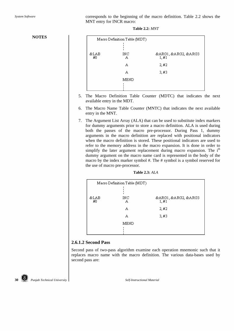
corresponds to the beginning of the macro definition. Table 2.2 shows the MNT entry for INCR macro:
Table 2.2: MNT
5. The Macro Definition Table Counter (MDTC) that indicates the next
available entry in the MDT.
6. The Macro Name Table Counter (MNTC) that indicates the next available entry in the MNT.
7. The Argument List Array (ALA) that can be used to substitute index markers for dummy arguments prior to store a macro definition. ALA is used during both the passes of the macro pre-processor. During Pass 1, dummy arguments in the macro definition are replaced with positional indicators when the macro definition is stored. These positional indicators are used to refer to the memory address in the macro expansion. It is done in order to simplify the later argument replacement during macro expansion. The ith dummy argument on the macro name card is represented in the body of the macro by the index marker symbol #. The # symbol is a symbol reserved for the use of macro pre-processor.
Table 2.3: ALA
2.6.1.2 Second Pass Second pass of two-pass algorithm examine each operation mnemonic such that it replaces macro name with the macro definition. The various data-bases used by second pass are:

Punjab Technical University 31
Macros and Macroprocessor
NOTES
Self-Instructional Material
1. The copy of the input macro source deck.
2. The output expanded source deck that can be used as an input to the assembler.
3. The MDT that was created by pass 1.
4. The MNT that was created by pass 1.
5. The MDTP for indicating the next line of text that is to be used during macro expansion.
6. The ALA that is used to substitute macro calls arguments for the index markers in the stored macro definition.
2.6.1.3 Two-Pass Algorithm In two-pass macro-preprocessor, you have two algorithms to implement, first pass and second pass. Both the algorithms examines line by line over the input data available. Two algorithms to implement two-pass macro-preprocessor are:
• Pass 1 Macro Definition • Pass 2 Macro Calls and Expansion
2.6.1.3.1 Pass 1 Macro Definition Pass 1 algorithm examines each line of the input data for macro pseudo opcode. Following are the steps that are performed during Pass 1 algorithm:
1. Intialize MDTC and MNTC with value one, so that previous value of MDTC and MNTC is set to value one.
2. Read the first input data.
3. If this data contains MACRO pseudo opcode then A. Read the next data input. B. Enter the name of the macro and current value of MDTC in MNT. C. Increase the counter value of MNT by value one. D. Prepare that argument list array respective to the macro found. E. Enter the macro definition into MDT. Increase the counter of MDT
by value one. F. Read next line of the input data. G. Substitute the index notations for dummy arguments passed in
macro. H. Increase the counter of the MDT by value one. I. If mend pseudo opcode is encountered then next source of input data
is read. J. Else expands data input.
4. If macro pseudo opcode is not encountered in data input then A. A copy of input data is created. B. If end pseudo opcode is found then go to Pass 2. C. Otherwise read next source of input data.
Figure 2.1 shows the above steps in diagrammatical structure:

32 Punjab Technical University
System Software
NOTES
Self-Instructional Material
Figure 2.1: Flow Chart for First Pass
Punjab Technical University 33
Macros and Macroprocessor
NOTES
Self-Instructional Material
2.6.1.3.2 Pass 2 Macro Calls and Expansion Pass two algorithm examines the operation code of every input line to check whether it exist in MNT or not. Following are the steps that are performed during second pass algorithm:
1. Read the input data received from Pass 1.
2. Examine each operation code for finding respective entry in the MNT.
3. If name of the macro is encountered then A. A Pointer is set to the MNT entry where name of the macro is found.
This pointer is called Macro Definition Table Pointer (MDTP). B. Prepare argument list array containing a table of dummy arguments. C. Increase the value of MDTP by value one. D. Read next line from MDT. E. Substitute the values from the arguments list of the macro for
dummy arguments. F. If mend pseudo opcode is found then next source of input data is
read. G. Else expands data input.
4. When macro name is not found then create expanded data file.
5. If end pseudo opcode is encountered then feed the expanded source file to assembler for processing.
6. Else read next source of data input.
Figure 2.2 shows the above steps followed to implement second pass algorithm in diagrammatical structure:

34 Punjab Technical University
System Software
NOTES
Self-Instructional Material
Figure 2.2: Flow Chart for Second Pass
2.6.2 Implementation of Single-Pass Algorithm The single-pass algorithm allows you to define macro within the macro but not supports macro calls within the macro. In the single-pass algorithm two additional

Punjab Technical University 35
Macros and Macroprocessor
NOTES
Self-Instructional Material
variables are used, Macro Definition Input (MDI) indicator and Macro Definition Level Counter (MDLC). Following is the usage of MDI and MDLC in single-pass algorithm:
• MDI indicator: Allows you to keep track of macro calls and macro definitions. During expansion of macro call, MDI indicator has value ON and retains value OFF otherwise. If MDI indicator is on, then input data lines are read from MDT until mend pseudo opcode is not encountered. When MDI is off, then data input is read from data source instead of MDI.
• MDLC indicator: MDLC ensures you that macro definition is stored in MDT. MDLC is a counter that keeps track of the numbers of macro1 and mend pseudo opcodes found.
Single-pass algorithm combines both the algorithms defined above to implement two-pass macro pre-processor. Following are the steps that are followed during single-pass algorithm:
1. Initialize MDTC and MNTC to value one and MDLC to zero. 2. Set MDI to value OFF. 3. Performs read operation. 4. Examine MNT to get the match with operation code. 5. If macro name is found then
A. MDI is set to ON. B. Prepare argument list array containing a table of dummy arguments. C. Performs read operation.
6. Else it examines that macro pseudo opcode is encountered. If macro pesudo opcode is found then
A. Enter the name of the macro and current value of MDTC in MNT at entry number MNTC.
B. Increment the MNTC to value one. C. Prepare argument list array containing a table of dummy arguments.. D. Enter the macro card into MDT. E. Increment the MDTC to value one. F. Increment the MDLC to value one. G. Performs read operation. H. Substitute the index notations for the arguments list of the macro for
dummy arguments. I. Enter data input line into MDT. J. Increment the MDTC to value one. K. If macro pseudo opcode is found then increments the MDLC to value
one and performs read operation. L. Else it checks for mend pseudo opcode if not found then performs
read operation. M. If mend pseudo opcode is found then decrement the MDLC to value
one. N. If MDLC is equal to zero then it goes to step 2. Otherwise, it
performs read operation. 7. In case macro pseudo opcode is not found, then write it into expanded source
card file.

36 Punjab Technical University
System Software
NOTES
Self-Instructional Material
If end pseudo opcode is found, then it feeds expanded source file to assembler for processing, otherwise performs read operation at step 2.
Figure 2.3: Single Pass
Figure 2.3 represents above steps in the pictorial representation using flow chart.
Check Your Progress 4. Which of the following is used
to store the name of the macro? A. MDT B. MNT C. MDLC D. MNTC
5. Which of the following is used to store the definition of the macro? A. MDT B. MNT C. MDLC D. MNTC
6. Which of the following is used to store the arguments of the macro? A. MDT B. MNT C. MDLC D. ALA

Punjab Technical University 37
Macros and Macroprocessor
NOTES
Self-Instructional Material
2.7 SUMMARY
This unit mainly focused on macro. It discussed how to define and expand a macro and about its various features including conditional macro expansion, macro instructions. In addition, it discussed the implementation of two-pass and single-pass macro pre-processor. 2.8 ANSWERS TO ‘CHECK YOUR PROGRESS’
1. Nested macro
2. Macros are abbreviations that can be replaced by instructions
3. Nested macro calls
4. MNT
5. MDT
6. ALA 2.9 EXERCISES AND QUESTIONS
Short-Answer Questions 1. What do you understand by macro ?
2. Describe macro expansion.
3. Explain nested macro calls.
4. Explain MNT and MDT.
Long-Answer Questions 1. Explain the features of macro facility in detail with examples.
2. Explain the following in detail: A. Implementation of single-pass macro pre-processor B. Nested macro class
2.10 FURTHER READING
Donovan, John J., Systems Programming.

38 Punjab Technical University
System Software
NOTES
Self-Instructional Material
UNIT 3 INTRODUCTION TO COMPILERS
Structure 3.0 Introduction 3.1 Unit Objectives 3.2 Compilers: An Overview
3.2.1 Cross Compiler; 3.2.2 One-Pass or Multi-pass Compiler; 3.2.3 Source-to-source Compiler; 3.2.4 Stage Compiler; 3.2.5 Just-in-time Compiler
3.3 Structure of a Compiler 3.3.1 Scanner; 3.3.2 Parser; 3.3.3 Symbol Tables and Error Handler; 3.3.4 Contextual Checkers; 3.3.5 Intermediate Code Generator; 3.3.6 Code Optimizer; 3.3.7 Code Generator; 3.3.8 Peep Hole Optimizer
3.4 Example of a Compiler 3.5 Phases of a Compiler
3.5.1 Lexical Analysis Phase; 3.5.2 Syntax Analysis Phase; 3.5.3 Intermediate Code Generation Phase; 3.5.4 Native Code Generation Phase; 3.5.5 Optimization Phase
3.6 Summary 3.7 Answers to ‘Check your Progress’ 3.8 Exercises and Questions 3.9 Further Reading 3.0 INTRODUCTION
A compiler is a very important part of the computer system, which helps an end user to translate the source code into the machine code. You need to use different phases of a compiler for an optimized output. Each phase of a compiler gives an output, which is used as the input for the next phase. 3.1 UNIT OBJECTIVES
• Discussing the basic concepts of a compiler • Understanding the various phases of a compiler • Understanding the operations associated with each phase of the compiler • Discussing operations that help optimize an output of a program
3.2 COMPILERS: AN OVERVIEW A compiler is a set of programs, which translates the text written in a computer language known as source language into another computer language known as target language. The text you input is called a source code and the output is called object code. You need to translate the source code to generate an executable program code. A compiler is generally used for programs that translate a source code written in a high level language to a lower level language, such as assembly language or machine language. A program that translates from lower level language to a higher level

Punjab Technical University 39
Introduction to Compilers
NOTES
Self-Instructional Material
language is known as a decompiler. A compiler performs various operations such as lexing, parsing, semantic analysis, code generation, code optimisation and preprocessing. Compilers are classified according to the input/output, internal structure and the behaviour at the run time. The various types of compiler that you can use are:
• Cross compilers • One-pass or multi-pass compiler • Source-to-source compiler • Stage compiler • Just-in-time compiler
3.2.1 Cross Compiler A cross compiler is a compiler that creates an executable code for one platform and runs the created executable code on another platform. A cross compiler helps separate the build environment from the target environment and is useful in a number of ways, such as it provides compiling for embedded systems and compiling an operating system for the first time.
3.2.2 One-pass or Multi-pass Compiler A compiler performs many operations and consumes a lot of memory space. So compilers are split into smaller programs that perform analysis and translations. A small program can be compiled in one pass while a big program is divided into a numbers of sub-programs, which is compiled in multiple times known as multi-pass. The ability to compile in one pass is beneficial because it simplifies the job of writing a compiler. One-pass compilers are faster than multi-pass compilers.
3.2.3 Source-to-source Compiler Source-to-source compilers are the compilers that take a high level language as its input and gives an output written in the same high level language.
3.2.4 Stage Compiler A stage compiler is used for compiling assembly language of a machine. For example, Warren Abstract Machine (WAM) is used as a stage compiler.
3.2.5 Just-in-time Compiler A just-in-time compiler allows you to deliver applications in byte code. For example, Smalltalk and Java systems use a just-in-time compiler. 3.3 STRUCTURE OF COMPILER
A typical compiler consists of various phases, such as lexical phase, parser phase, contextual analysis phase, optimisation phase and code generation phase. The phases of the compiler allow you to pass the output of the phase to the next phase. Figure 3.1 shows the structure of a compiler that takes input as the source code and gives output as the target code.

40 Punjab Technical University
System Software
NOTES
Self-Instructional Material
Figure 3.1: Structure of a Compiler
3.3.1 Scanner The scanner allows you to group the input characters into tokens and construct a symbol table that is used for contextual analysis of the program code in the later phase. The tokens are also known as lexemes, which include:
• Keyword • Identifier • Operators • Constants • Comments
The scanner phase is also known as lexical phase that helps group input characters into lexical units or tokens. The output of the lexical phase is a stream of tokens.
3.3.2 Parser The parser helps group tokens into syntactical units. The output you get from the parser phase is a parse tree, which is a tree representation of a program. The program structure you get from the parser phase is defined using context-free grammars, which is defined by the following five components:

Punjab Technical University 41
Introduction to Compilers
NOTES
Self-Instructional Material
• A finite terminal vocabulary Vt , which is a token produced by a scanner • A finite set of symbols known as the non-terminal vocabulary Vn • A start symbol S for the grammer • A finite set of productions, P • Push down automata
3.3.3 Symbol Tables and Error Handler The additional information that you acquire during any phase of the compiler and which you can use in the later phase is stored in symbol tables. The information that you store can be a name encountered in the source program or an attribute. The error handler helps report and rectify an error that occurs during the execution of the source program.
3.3.4 Contextual Checkers You use context checkers to analyse the parse tree for context sensitive information, which is known as static semantics. The output of the semantic analysis phase is an annotated parse tree.
3.3.5 Intermediate Code Generator The data structure that you pass between the synthesis and analysis phase is called Intermediate Representation (IR) of the program. The intermediate representation in a source program can be:
• Assembly language
• Abstract syntax tree
3.3.6 Code Optimizer The reconstruction of a parse tree to reduce the size of the tree or to reproduce an equivalent tree that gives more efficient code is known as a code optimizer. Following example shows the use of code optimisation:
• Constant folding: Constant folding allows you to reduce calculation in a program code as shown in the example:
• Loop-constant code motion: Loop-constant code motion helps reduce the
calculation inside a loop as shown in the example:

42 Punjab Technical University
System Software
NOTES
Self-Instructional Material
• Induction variable reduction: During the execution of a program code,
most of the processing time is spent in the body of the loops. Induction variable reduction helps in the improvement of the performance by reducing the execution time inside a loop. The following example shows the use of induction variable reduction.
• Common sub-expression elimination: The common expression that occur
in a source code are eliminated for reducing redundancy, this is done using common sub-expression elimination method. The following code shows the use of common sub-expression elimination.
• Strength reduction: Strength reduction helps reduce the calculation of
operator, such as addition and subtraction.
3.3.7 Code Generator The task of the code generator is to translate the intermediate representation of the source code into the code of the target machine. The code of the target machine can

Punjab Technical University 43
Introduction to Compilers
NOTES
Self-Instructional Material
be binary, assembly or any high level language. A code generator can also be integrated with a parser.
3.3.8 Peep Hole Optimizer A peep hole optimizer allows you to scan small segments of the target code that helps improve efficiency of the instructions in a program code. Peep hole optimization is the last phase of the compilation process, which helps you to discard redundant instructions in the program code. 3.4 EXAMPLE OF A COMPILER
The following example shows how to use a one-pass compiler, which is written in C programming language.
#include <stdlib.h> #include <stdio.h> #include <string.h> #define MODE_POSTFIX 0 #define MODE_ASSEMBLY 1 char lookahead; int pos; int compile_mode; char expression[20+1]; void error() { printf("Syntax error!\n"); } void match( char t ) { if( lookahead == t ) { pos++; lookahead = expression[pos]; } else error(); } void digit() { switch( lookahead ) { case '0': case '1': case '2': case '3': case '4': case '5':
case '6':
case '7': case '8': case '9':
if( compile_mode == MODE_POSTFIX ) printf("%c", lookahead); else printf("\tPUSH %c\n", lookahead);
Check Your Progress 1. The input of a cross compiler
gives an output on ……. computer.
2. What happens when an error is encountered during the execution of a program?
3. Which compiler gives a high level language as output?

44 Punjab Technical University
System Software
NOTES
Self-Instructional Material
match( lookahead ); break; default: error(); break; } } void term() { digit(); while(1) { switch( lookahead ) { case '*': match('*'); digit(); printf( "%s", compile_mode == MODE_POSTFIX ? "*" : "\tPOP B\n\tPOP A\n\tMUL A, B\n\tPUSH A\n"); break; case '/': match('/'); digit(); printf( "%s", compile_mode == MODE_POSTFIX ? "/" : "\tPOP B\n\tPOP A\n\tDIV A, B\n\tPUSH A\n"); break; default: return; } } } void expr() { term(); while(1) { switch( lookahead ) { case '+': match('+'); term(); printf( "%s", compile_mode == MODE_POSTFIX ? "+" : "\tPOP B\n\tPOP A\n\tADD A, B\n\tPUSH A\n"); break; case '-':
match('-'); term(); printf( "%s", compile_mode == MODE_POSTFIX ? "-" : "\tPOP B\n\tPOP A\n\tSUB A, B\n\tPUSH A\n"); break; default:
return; }

Punjab Technical University 45
Introduction to Compilers
NOTES
Self-Instructional Material
}
} int main ( int argc, char** argv ) { printf("Please enter an infix-notated expression with single digits:\n\n\t"); scanf("%20s", expression); printf("\nCompiling to postfix-notated expression:\n\n\t"); compile_mode = MODE_POSTFIX; pos = 0; lookahead = *expression; expr(); printf("\n\nCompiling to assembly-notated machine code:\n\n"); compile_mode = MODE_ASSEMBLY; pos = 0; lookahead = *expression; expr(); return 0; }
The result of the compiler is the following output: Please enter an infix-notated expression with single digits: 3-4*2+2 Compiling to postfix-notated expression: 342*-2+
Compiling to assembly-notated machine code: PUSH 3 PUSH 4 PUSH 2 POP B POP A MUL A, B PUSH A POP B POP A SUB A, B PUSH A PUSH 2 POP B POP A ADD A, B PUSH A

46 Punjab Technical University
System Software
NOTES
Self-Instructional Material
3.5 PHASES OF A COMPILER
A compiler is broken into several logical phases that help in the execution of a source code with efficiency to improve the performance of the compiler. The common logical phases that you use in a compiler for translating a source code into the target code are:
• Lexical analysis phase • Syntax analysis phase • Intermediate code generation phase • Native code generation phase • Optimization phase
3.5.1 Lexical Analysis Phase Lexical analysis phase allows you to perform the sequencing of input characters such as the source code of a computer program, and produces an output known as lexical tokens. The lexical tokens can be used as the input for the next phase such as a parser phase. A lexical analysis phase is a combination of two stages:
• A scanner: Is based on a finite state machine and provides information, such as a possible sequence of characters that a token can contain.
• An evaluator: Contains information about the characters of the lexeme to produce a value. A lexeme is a string of characters that contains string of a certain type. A token is a combination of a lexeme and its corresponding value, which is used as an input for the parser. For example, the source code of a program contains a string and the string is converted into a lexical token stream. The string: net_worth_future = ( assets_responsibilities ) ; Lexical token stream: NAME “net_worth_future” EQUALS OPEN_PARENTHESIS NAME “assets” MINUS NAME “responsibilities” CLOSE_PARENTHESIS SEMICOLON
The lexical token streams are generated using automated tools that accept regular expressions. A regular expression is simply a string of characters that defines a pattern used to search for a matching string. The automated tools generate source code that can be compiled and executed and helps construct a state table for a finite state machine. Regular expressions represent expressions, such as English based language, ASCII alphanumeric character and an underscore.

Punjab Technical University 47
Introduction to Compilers
NOTES
Self-Instructional Material
3.5.1.1 Symbols Used in Lexical Analysis Phase This is an example of a scanner, which is written in C programming language and describes various tokens, keywords, numbers and identifiers for the instructional programming language.
• The symbols recognized are: +, -, *, /, =, (, ), :=, <, <, <>, >, >=, ; • The number are: 0-9 • The identifiers are: a-z and A-Z • Keywords used are: begin, call, const, do, end, if, odd, procedure, then, var,
while • External variables used:
FILE *source — the source file int cur_line, cur_col, err_line, err_col — for error reporting int num -- last number read stored here, for the parser char id[]— last identifier read stored here, for the parser Hashtab *keywords — list of keywords
• External routines called: error(const char msg[]) — report an error Hashtab *create_htab(int estimate) — create a lookup table int enter_htab(Hashtab *ht, char name[], void *data) — add an entry
to a lookup table Entry *find_htab(Hashtab *ht, char *s) — find an entry in a lookup
table void *get_htab_data(Entry *entry) — returns data from a lookup
table FILE *fopen(char fn[], char mode[]) — opens a file for reading fgetc(FILE *stream) — read the next character from a stream ungetc(int ch, FILE *stream) — putback a character onto a stream isdigit(int ch), isalpha(int ch), isalnum(int ch) — character
classification • External types:
o Symbol -- an enumerated type of all the symbols. o Hashtab -- represents a lookup table o Entry -- represents an entry in the lookup table
Scanning is started by calling init_scan, which helps pass the name of the source code file. If the source file is successfully opened, the parser calls getsym repeatedly to return successive symbols from the source file.
3.5.2 Syntax Analysis Phase Syntax analysis phase helps you to recognise the structure of the programming language, also known as parsing. Syntax analysis is performed after lexical analysis that helps to write and use a parser. The programs or code that perform parsing are called parsers.
3.5.3 Intermediate Code Generation Phase The intermediate code generation phase translates the source code into target code. An intermediate code is generated when a direct target code is not desired. The two
Check Your Progress 4. How does the intermediate
code generator work? 5. What are lexemes? 6. Which of these is a keyword?
A. for B. next C. end D. exit

48 Punjab Technical University
System Software
NOTES
Self-Instructional Material
main reasons, which are responsible for the generation of an intermediate code rather than generating a direct target code, are:
• The intermediate form is a simple version of the cource code that helps an optimizer to apply the optimizations, such as common sub-expression elimination and strength reduction.
• Many compilers, such as cross compilers generate target code for many CPUs.
The lexical analysis phase or the parser phase obtains the input and calls the intermediate code generator for processing the parser’s output.
3.5.4 Native Code Generation Phase After intermediate code generation, the next phase in the generation of target code is native code generation. In native code generation phase, the intermediate code generated in the previous phase is converted into a code, which is understandable to the processor installed on a particular computer. Such code that a computer understands for performing a particular task is known as native code.
3.5.5 Optimization Phase The optimization phase translates the intermediate code into a more efficient form, which involves eliminating repeated and unnecessary entries from the input code. Following example shows how to apply optimization on an intermediate code:
3.6 SUMMARY
A compiler is responsible for the execution of a program code that helps to translate the source code into the machine code. The basic structure of a compiler contains a lexer, a parser, a code generator and an optimizer, which helps specify the basic design of a compiler.
3.7 ANSWERS TO ‘CHECK YOUR PROGRESS’
1. Another.
2. The error handler checks for the error encountered and gives instructions to recover from the error.
3. Source-to-source compiler.
4. An intermediate code generator takes an input from the syntax analyser and applies optimization on the input to produce an output that uses CPU efficiently.

Punjab Technical University 49
Introduction to Compilers
NOTES
Self-Instructional Material
5. Lexemes are the tokens that you get after the lexical analysis phase ends.
6. end
3.8 EXERCISES AND QUESTIONS
Short-Answer Type Questions 1. What is the difference between a compiler and an interpreter?
2. What is type checking?
3. Which compiler should be used for faster execution of programs, and why?
4. Explain the syntax analysis phase?
Long-Answer Type Questions 1. What is a parse tree and how is it represented?
2. What is the output of the following expression after lexical analysis:
Position: = initial + rate*50; 3.9 FURTHER READING
Dhamdhere, D. M., Systems Programming and Operating Systems.
Donovan, John J., Systems Programming, Tata McGraw-Hill Edition.

50 Punjab Technical University
System Software
NOTES
Self-Instructional Material
UNIT 4 LOADERS AND LINKAGE EDITORS
Structure 4.0 Introduction 4.1 Unit Objectives 4.2 Loaders and Linkers: An Overview
4.2.1 Object Modules; 4.2.2 Binary Programs 4.3 Loaders
4.3.1 Compile and Go Loader; 4.3.2 Absolute Loader; 4.3.3 Relocating Loaders; 4.3.4 Direct-Linking Loaders
4.4 Linkage Editor 4.4.1 Program Relocation; 4.4.2 Program Linking
4.5 Design of a Linker 4.5.1 First Pass; 4.5.2 Second Pass
4.6 Dynamic Linking 4.7 Bootstrap Loader 4.8 Summary 4.9 Answers to ‘Check your Progress’ 4.10 Exercises and Questions 4.11 Further Reading 4.0 INTRODUCTION
Earlier programmers used loaders that could take program routines stored in tapes and combine and relocate them in one program. Later, these loaders evolved into linkage editor used for linking the program routines but the program memory remained expensive and computers were slow. A little progress in linking technology helped computers become faster and disks larger, thus program linking became easier. For the easier use of memory space and efficiency in speed, you need to use linkers and loaders. 4.1 UNIT OBJECTIVES
• Discussing the basic components of loaders and linkers • Understanding various loader schemes for loading a progarm • Understanding the working and design of a linker • Understanding the concept of a bootstrap loader and how it is loaded in the
operating system 4.2 LOADERS AND LINKERS: AN OVERVIEW
An overview of loaders and linkers helps you to have a schematic flow of steps that you need to follow while creating a program. Following are the steps that you need to perform when you write a program in language:

Punjab Technical University 51
Loaders and Linkers Editors
NOTES
Self-Instructional Material
1. Translation of the program, which is performed by a processor called translator.
2. Linking of the program with other programs for execution, which is performed by a separate processor known as linker.
3. Relocation of the program to execute from the memory location allocated to it, which is performed by a processor called loader.
4. Loading of the program in the memory for its execution, which is performed by a loader.
Figure 4.1 shows a schematic flow of program execution, in which a translator, linker and loader performs functions such as translating and linking a program for the final result of the program.
Figure 4.1: Schematic Flow of Program Execution
4.2.1 Object Modules The object module of a program contains information, which is necessary to relocate and link the program with other programs. The object module of a program, P, consists of various components:
1. Header contains translated origin, size and execution start address of the program P. Translated origin is the address of the origin assumed by the translator.
2. Program contains the machine language program corresponding to P. 3. Relocation table(RELOCTAB) maintains a list of entries that contains the
translated address for the corresponding entry. 4. Linking table(LINKTAB) contains information about the external
references and public definitions of the program P.
4.2.2 Binary Programs A binary program is a machine language program, which contains a set of program units P where Pi ε P. Pi has a memory address that is relocated at its link origin. Link origin is the address of the origin assigned by the linker while producing a binary program. You need to invoke a linker command for creating a binary program from a set of object modules. The syntax for the linker command is:

52 Punjab Technical University
System Software
NOTES
Self-Instructional Material
linker <link origin>, <object module names>,[<execution start address>]
4.3 LOADERS
As already discussed that assemblers and compilers are used to convert the source program developed by the user to the corresponding object program. A loader is a program that performs the functions of a linker program and then immediately schedules the resulting executable program for some kind of action. In other words, a loader accepts the object program, prepares these programs for execution by the computer and then initiates the execution. It is not necessary for the loader to save a program as an executable file. The functions performed by a loader are as follows:
1. Memory Allocation allocates space in memory for the program.
2. Linking: Resolves symbolic references between the different objects.
3. Relocation adjusts all the address dependent locations such as address constants, in order to correspond to the allocated space.
4. Loading places the instructions and data into memory.
The concept of loaders can be well understood if one knows the general loader scheme. It is recommended for the general loader scheme that the instructions and data should be produced in the output, as they were assembled. This strategy, if followed, prevents the problem of wasting core for an assembler. When the code is required to be executed, the output is saved and loaded in the memory. The assembled program is loaded into the same area in core that it occupied earlier. The output that contains a coded form of the instructions is called the object deck. The object deck is used as intermediate data to avoid the circumstances in which the addition of a new program to a system is required. The loader accepts the assembled machine instructions, data and other information present in the object. The loader places the machine instructions and data in core in an executable computer form.
More memory can be made available to a user, since in this scheme, the loader is assumed to be smaller than the assembler. Figure 4.2 shows the general loader scheme.
Figure 4.2: The General Loader Scheme

Punjab Technical University 53
Loaders and Linkers Editors
NOTES
Self-Instructional Material
There are various other loading schemes such as compile and go loader, absolute loader, relocating loader and direct linking loader.
4.3.1 Compile and Go Loader Compile and go loader is also known as “assembler-and-go”. It is required to introduce the term “segment” to understand the different loader schemes. A segment is a unit of information such as a program or data that is treated as an entity and corresponds to a single source or object deck. Figure 4.3 shows the compile and go loader.
The compile and go loader executes the assembler program in one part of memory and places the assembled machine instructions and data directly into their assigned memory locations. Once the assembly is completed, the assembler transfers the control to the starting instruction of the program.
Figure 4.3: The Compile and Go Loader Scheme
This scheme is easy to implement, as the assembler simply places the code into core and the loader, which consists of one instruction, transfers control to the starting instruction of the newly assembled program. However, this scheme has several disadvantages. First, in this scheme, a portion of memory is wasted. This is mainly because the core occupied by the assembler is not available to the object program. Second, it is essential to assemble the user’s program deck every time it is executed. Finally, it is quite difficult to handle multiple segments, if the source programs are in different languages. This disadvantage makes it difficult to produce orderly modular programs.
4.3.2 Absolute Loader An absolute loader is the simplest type of loader scheme that fits the general model of loaders. The assembler produces the output in the same way as in the “compile and go loader”. The assembler outputs the machine language translation of the source program. The difference lies in the form of data, i.e., the data in the absolute loader is punched on cards or you can say that it uses object deck as an intermediate data. The
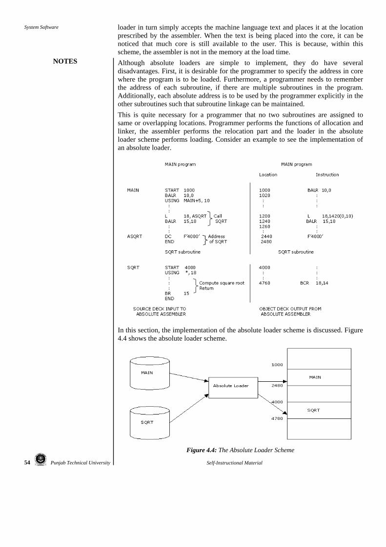
54 Punjab Technical University
System Software
NOTES
Self-Instructional Material
loader in turn simply accepts the machine language text and places it at the location prescribed by the assembler. When the text is being placed into the core, it can be noticed that much core is still available to the user. This is because, within this scheme, the assembler is not in the memory at the load time. Although absolute loaders are simple to implement, they do have several disadvantages. First, it is desirable for the programmer to specify the address in core where the program is to be loaded. Furthermore, a programmer needs to remember the address of each subroutine, if there are multiple subroutines in the program. Additionally, each absolute address is to be used by the programmer explicitly in the other subroutines such that subroutine linkage can be maintained. This is quite necessary for a programmer that no two subroutines are assigned to same or overlapping locations. Programmer performs the functions of allocation and linker, the assembler performs the relocation part and the loader in the absolute loader scheme performs loading. Consider an example to see the implementation of an absolute loader.
In this section, the implementation of the absolute loader scheme is discussed. Figure 4.4 shows the absolute loader scheme.
Figure 4.4: The Absolute Loader Scheme

Punjab Technical University 55
Loaders and Linkers Editors
NOTES
Self-Instructional Material
In the figure, the MAIN program is assigned to locations 1000-2470 and the SQRT subroutine is assigned locations 4000-4770. This means the length of MAIN has increased to more than 3000 bytes, as it can be noticed from figure 4.4. If the modifications are required to be made in MAIN subroutine, then the end of MAIN subroutine, i.e., 1000+3000=4000, gets overlapped with the start of SQRT, i.e., with 4000. Therefore, it is necessary to assign a new location to SQRT. This can be made possible by changing the START pseudo-op card and reassembling it. It is then quite obvious to modify all other subroutines that refer to address of SQRT.
4.3.3 Relocating Loaders Relocating loaders was introduced in order to avoid possible reassembling of all subroutines when a single subroutine is changed. It also allows you to perform the tasks of allocation and linking for the programmer. The example of relocating loaders includes the Binary Symbolic Subroutine (BSS) loader. Although the BSS loader allows only one common data segment, it allows several procedure segments. The assembler in this type of loader assembles each procedure segment independently and passes the text and information to relocation and intersegment references.
In this scheme, the assembler produces an output in the form of text for each source program. A transfer vector that contains addresses, which includes names of the subroutines referenced by the source program, prefixes the output text. The assembler would also provide the loader with additional information such as the length of the entire program and also the length of the transfer vector portion. Once this information is provided, the text and the transfer vector get loaded into the core. Followed by this, the loader would load each subroutine, which is being identified in the transfer vector. A transfer instruction would then be placed to the corresponding subroutine for each entry in the transfer vector.
The output of the relocating assembler is the object program and information about all the programs to which it references. Additionally, it also provides relocation information for the locations that need to be changed if it is to be loaded in the core. This location may be arbitrary in the core, let us say the locations, which are dependent on the core allocation. The BSS loader scheme is mostly used in computers with a fixed-length direct-address instruction format. Consider an example in which the 360 RX instruction format is as follows:
In this format, A2 is the 16-bit absolute address of the operand, which is the direct address instruction format. It is desirable to relocate the address portion of every instruction. As a result, the computers with a direct-address instruction format have much severe problems than the computes having 360-type base registers. The 360-type base registers solve the problem using relocation bits. The relocation bits are included in the object desk and the assembler associates a bit with each instruction or address field. The corresponding address field to each instruction must be relocated if the associated bit is equal to one; otherwise this field is not relocated.
4.3.4 Direct-Linking Loaders A direct-linking loader is a general relocating loader and is the most popular loading scheme presently used. This scheme has an advantage that it allows the programmer

56 Punjab Technical University
System Software
NOTES
Self-Instructional Material
to use multiple procedure and multiple data segments. In addition, the programmer is free to reference data or instructions that are contained in other segments. The direct-linking loaders provide flexible intersegment referencing and accessing ability. An assembler provides the following information to the loader along with each procedure or data segment. This information includes:
• Length of segment. • List of all the symbols and their relative location in the segment that are
referred by other segments. • Information regarding the address constant which includes location in
segment and description about the revising their values. • Machine code translation of the source program and the relative addresses
assigned.
Let us understand the implementation of the direct-linking loader with the help of an example. In the following example, there is a source program, which is being translated by an assembler in order to produce the object code. The source program and the object code, which is being translated, both are depicted code and their var.
You must have noticed that the card number 15 in the example contains a Define Constant (DC) pseudo operation that provide instructions to the assembler. This pseudo-op helps in creating a constant with the value that contains the address of TABLE, which places this constant value at the location labelled as POINTER.
This is the point where the assembler does not know the final absolute address of TABLE. This is because the assembler does not have any idea where the program is to be loaded. However, the assembler has the knowledge that address of TABLE is 28th byte from the beginning of the program. Therefore, the assembler places 28 in POINTER. It also informs to the loader that if this program gets loaded at some other location, other than absolute location 0, then the content of location POINTER is incorrect.

Punjab Technical University 57
Loaders and Linkers Editors
NOTES
Self-Instructional Material
Another usage of DC pseudo-op in this program is on card number 17. This pseudo-op instructs the assembler to create a constant with the value of the address of the subroutine ADD. It would also cause this constant to be placed in the location, which is labelled as AADD. The assembler cannot generate this constant, as the assembler does not have any idea of the location where the procedure ADD is loaded. It is desirable for the assembler to provide information to the loader such that the final absolute address of ADD can be loaded at the designated location, i.e., AADD, when the program gets loaded. 4.4 LINKAGE EDITOR
Linkage editor allows you to combine two or more objects defined in a program and supply information needed to allow references between them. A linkage editor is also known as linker. To allow linking in a program, you need to perform:
• Program relocation • Program linking
4.4.1 Program relocation Program relocation is the process of modifying the addresses containing instructions of a program. You need to use program relocation to allocate a new memory address to the instruction. Instructions are fetched from the memory address and are followed sequentially to execute a program. The relocation of a program is performed by a linker and for performing relocation you need to calculate the relocation_factor that helps specify the translation time address in every instruction. Let the translated and linked origins of a program P be t_origin and l_origin, respectively. The relocation factor of a program P can be defined as:
relocation_factor = l_origin – t_origin
The algorithm that you use for program relocation is:
1. program_linked_origin:=<link origin> from linker command;
2. For each object module
3. t_origin :=translated origin of the object module; OM_size :=size of the object module;
4. relocation_factor :=program_linked_origin-t_origin;
5. Read the machine language program in work_area;
6. Read RELOCTAB of the object module
7. For each entry in RELOCTAB A. translated_addr: = address in the RELOCTAB entry; B. address_in_work: =address of work_area + translated_address –
t_origin; C. add relocation_factor to the operand in the wrd with the address
address_in_work_area. D. program_linked_origin: = program_linked_origin + OM_size;

58 Punjab Technical University
System Software
NOTES
Self-Instructional Material
4.4.2 Program Linking Linking in a program is a process of binding an external reference to a correct link address. You need to perform linking to resolve external reference that helps in the execution of a program. All the external references in a program are maintained in a table called name table (NTAB), which contains the symbolic name for external references or an object module. The information specified in NTAB is derived from LINKTAB entries having type=PD. The algorithm that you use for program linking is:
Algorithm (Program Linking)
1. program_linked_origin: =<link origin> from linker command.
2. for each object module A. t_origin: =translated origin of the object module;
OM_size :=size of the object module; B. relocation_factor: =program_linked_origin – t_origin; C. read the machine language program in work_area. D. Read LINKTAB of the object module. E. For each LINKTAB entry with type=PD
name: =symbol; linked_address: =translated_address + relocation_factor; Enter ( name, linked_address) in NTAB.
F. Enter (object module name, program_linked_origin) in NTAB. G. Program_linked_origin: = program_linked_origin + OM_size;
3. for each object module A. t_origin: =translated origin of the object module;
program_linked_origin :=load_address from NTAB; B. for each LINKTAB entry with type=EXT
address_in_work_area: =address of work_area + program_linked_origin - <link origin> + translated address – t_origin
search symbol in NTAB and copy its linked address. Add the linked address to the operand address in the word with the address address_in_work_area.
4.5 DESIGN OF A LINKER
You need to perform linking and relocation to explain the design of a linker. For example, the design of a program LINKER helps explain linking and relocation. The output of a LINKER program is in binary form with a .COM extension. You need to use the following syntax to create a LINKER program:
LINKER <object module name>,<executable file>,<load origin>,<list of binary files>
The LINKER program allows you to perform linking and relocation of all the named object modules, which are contained in <object module name>. The program is
Check Your Progress 1. How many object module
names can be specified in a linker command?
2. Can a RELOCTAB contain an original link address?
3. How can you specify an array of namelist in a program?
Punjab Technical University 59
Loaders and Linkers Editors
NOTES
Self-Instructional Material
stored in <executable file>, the <list of binary files> contains a list of external object module name that are not specified in <object module name>. You need to resolve all the external object module names for terminating the execution of LINKER program. The LINKER program is explained using an example:
LINKER alpha+beta+min, calculate, 1000, pas.lib
Alpha, beta and min are the names of the object modules that you need to link, and calculate is the name given to the executable file, which is generated by LINKER. The load origin of the program that you want to execute is 1000. The external names, which are not defined in object modules alpha, beta and min needs to be searched in pas.lib library
For proper execution of the LINKER program you need to use a two-pass strategy: • First pass • Second pass
4.5.1 First Pass In the first pass, the object module collects information about the segments and definitions that are defined in the program. The algorithm that you use for the first pass is:
Algorithm (first pass of LINKER)
1. Program_linked_origin: =<load origin>; // a default value is used if <load origin is not specified>.
2. Repeat step 3 for each object module to be linked.
3. Select an object module and process its object records. A. If an LANAME record, enter the names in NAMELIST. B. If a SEGDEF record
i: = name index; segment_name := NAMELIST[i]; segment_addr: =start address in attributes(if present); If an absolute segment, enter (segment_name,
segment_addr) in NTAB. If segment is relocatable and cannot be combined with other
segments: -align the address contained in program_linked_origin on the next word or paragraph as indicated in the attributes field. -enter (segment_name, program_linked_origin) in NTAB. -program_linked_origin :=program load origin+segment length;
C. For each PUBDEF record i:=base; segment_name := NAMELIST[i]; symbol:=name; segment_addr:=load address of segment_name in NTAB; sym_addr:=segment_addr+offset; Enter (symbol, sym_addr) in NTAB.

60 Punjab Technical University
System Software
NOTES
Self-Instructional Material
4.5.2 Second Pass The second pass performs relocation and linking of the program. Second pass helps execute program in work_area. You need to fetch the data from LEDATA records using segment index and data offset and send them to the correct parts of work_area. The segment index helps obtain the load origin of the segment from NTAB while data offset gives the load address of the first byte of the data in the LEDATA record. A segment index can also contain a numeric value rather than the name of the segment, LNAMES records help obtain the segment name. The obtained segment name, the segment name is searched in NTAB for its load origin. For the relocation and linking you need to FIXUPP records, while processing a FIXUPP the target data can be searched in EXTDEF or SEGDEF to obtain the target name. The obtained target name can be searched in NTAB for its load origin. LINKER constructs a table called the segment table (SEGTAB), which contains the name of all the segments defined in the object module. A SEGTAB entry has the following syntax:
The information about the load address is copied from NTAB.
For the relocation and linking, you need to FIXUPP records, while processing a FIXUPP the target data can be searched in EXTDEF or SEGDEF to obtain the target name. The obtained target name can be searched in NTAB for its load origin. A FIXUPP record may also contain a reference to an external symbol, LINKER constructs an external symbols table (EXTTAB), which has the following syntax:
The information about the load address is copied from NTAB.
At the end of the second pass, the executable program is stored in <executable file>, which is specified in the LINKER command.
The algorithm that you use for the second pass is:
1. list_of_object_modules: = object modules named in LINKER command;
2. Repeat step 3 until list_of_object_modules is empty.
3. Select an object module and process its object records. A. If an LNAMES record
Enter the names in NAMELIST. B. If a SEGDEF record
i:= name index; segment_name :=NAMELIST[i] ; Enter (segment_name, load address from NTAB) in SEGTAB.
C. If an EXTTAB record external_name: =name from EXTTAB record; If external_name is not found in NTAB, then
-Locate an object module in the library which contains external_name as a segment or public definition. -Add name of object module to list_of_object_modules. -Perform first pass of LINKER, for the new object module.
Punjab Technical University 61
Loaders and Linkers Editors
NOTES
Self-Instructional Material
Enter (external_name, load address from NTAB) in EXTTAB
D. If an LEDATA record i := segment index; d:=data offset; program_load_origin:=SEGTAB[i].load address; address_in_work_area:= address of work_area +
program_load_origin-<load origin> + d; Move the data from LEDATA into the memory area starting
at the address address_in_work_area. E. If a FIXUPP record, for each FIXUPP specification
f:=offset from locat field; fix_up_address:= address in work_area + f; perform required fix up using a load address from SEGTAB
or EXTTAB and the value of the code in locat and fix dat. F. If a MODEND record
If start address is specified, compute the corresponding load address (analogous to the computation while processing an LEDATA record) and record it in the executable file being generated.
4.6 DYNAMIC LINKING
Sophisticated operating systems, such as Windows allow you to link executable object modules to be linked to a program while a program is running. This is known as dynamic linking. The operating system contains a linker that determines functions, which are not specified in a progam. A linker searches through the specified libraries for the missing function and helps extract the object modules containing the missing functions from the libraries. The libraries are constructed in a way to be able to work with dynamic linkers. Such libraries are known as dynamic link libraries (DLLs). Technically, dynamic linking is not like static linking, which is done at build time. DLLs contain functions or routines, which are loaded and executed when needed by a program. The advantages of DLLs are:
• Code sharing: Programs in dynamic linking can share an identical code instead of creating an individual copy of a same library. Sharing allows executable functions and routines to be shared by many application programs. For example, the object linking and embedding (OLE) functions of OLE2.DLL can be invoked to allow the execution of functions or routines in any program.
• Automatic updating: Whenever you install a new version of dynamic link library, the older version is automatically overridden. When you run a program the updated version of the dynamic link library is automatically picked.
• Securing: Splitting the program you create into several linkage units makes it harder for crackers to read an executable file.
4.7 BOOTSTRAP LOADER Bootstrap is a very small program that usually reside in Read Only Memory (ROM), which reads fixed locations from the disk on an operating system. The bootstrap

62 Punjab Technical University
System Software
NOTES
Self-Instructional Material
program is loaded in the memory that helps understand how a computer operates. Bootstrap is a short program loaded by the BIOS when the system starts up. The BIOS does not specify any information about the environment an operating system needs and thus is not able to initialize a system. Some of the BIOS boot devices include:
• Primary input devices such as keyboard • Primary output devices such as monitor • Initial program load device such as floppy drive, hard drive, CD-ROM, USB
and flash drive
It is the responsibility of the bootstrap loader to load the code and build an appropriate operating environment. Bootstrap programs are capable of performing various tasks such as initialising certain pieces of hardware, putting the processor into advanced operating modes or performing a dedicated processing task. The bootstrap loader locate the files to start an operating system, to locate the target files you need to understand the file allocation table (FAT) system. FAT contains a sequence of files and helps load the files into memory. The following source code shows how to search for a file, load the file into the memory and begin the execution of the loaded file.
[BITS 16] ORG 0 jmp START OEM_ID db "QUASI-OS" BytesPerSector dw 0x0200 SectorsPerCluster db 0x01 ReservedSectors dw 0x0001 TotalFATs db 0x02 MaxRootEntries dw 0x00E0 TotalSectorsSmall dw 0x0B40 MediaDescriptor db 0xF0 SectorsPerFAT dw 0x0009 SectorsPerTrack dw 0x0012 NumHeads dw 0x0002 HiddenSectors dd 0x00000000 TotalSectorsLarge dd 0x00000000 DriveNumber db 0x00 Flags db 0x00 Signature db 0x29 VolumeID dd 0xFFFFFFFF VolumeLabel db "QUASI BOOT" SystemID db "FAT12 " START: ; code located at 0000:7C00, adjust segment registers cli mov ax, 0x07C0 mov ds, ax mov es, ax mov fs, ax mov gs, ax ; create stack mov ax, 0x0000 mov ss, ax mov sp, 0xFFFF sti

Punjab Technical University 63
Loaders and Linkers Editors
NOTES
Self-Instructional Material
; post message mov si, msgLoading call DisplayMessage LOAD_ROOT: ; compute size of root directory and store in "cx" xor cx, cx xor dx, dx
mov ax, 0x0020 ; 32 byte directory entry mul WORD [MaxRootEntries] ; total size of directory div WORD [BytesPerSector] ; sectors used by directory xchg ax, cx ; compute location of root directory and store in "ax" mov al, BYTE [TotalFATs] ; number of FATs mul WORD [SectorsPerFAT] ; sectors used by FATs add ax, WORD [ReservedSectors] ; adjust for bootsector mov WORD [datasector], ax ; base of root directory add WORD [datasector], cx ; read root directory into memory (7C00:0200) mov bx, 0x0200 ; copy root dir above bootcode call ReadSectors ; browse root directory for binary image mov cx, WORD [MaxRootEntries] ; load loop counter mov di, 0x0200 ; locate first root entry .LOOP: push cx mov cx, 0x000B ; eleven character name mov si, ImageName ; image name to find push di rep cmpsb ; test for entry match pop di je LOAD_FAT pop cx add di, 0x0020 ; queue next directory entry loop .LOOP jmp FAILURE LOAD_FAT: ; save starting cluster of boot image mov si, msgCRLF call DisplayMessage mov dx, WORD [di + 0x001A] mov WORD [cluster], dx ; file's first cluster

64 Punjab Technical University
System Software
NOTES
Self-Instructional Material
; compute size of FAT and store in "cx" xor ax, ax mov al, BYTE [TotalFATs] ; number of FATs mul WORD [SectorsPerFAT] ; sectors used by FATs mov cx, ax ; compute location of FAT and store in "ax" mov ax, WORD [ReservedSectors] ; adjust for bootsector
; read FAT into memory (7C00:0200) mov bx, 0x0200 ; copy FAT above bootcode call ReadSectors ; read image file into memory (0050:0000) mov si, msgCRLF call DisplayMessage mov ax, 0x0050 mov es, ax ; destination for image mov bx, 0x0000 ; destination for image push bx LOAD_IMAGE: mov ax, WORD [cluster] ; cluster to read pop bx ; buffer to read into call ClusterLBA ; convert cluster to LBA xor cx, cx mov cl, BYTE [SectorsPerCluster] ; sectors to read call ReadSectors push bx ; compute next cluster mov ax, WORD [cluster] ; identify current cluster mov cx, ax ; copy current cluster mov dx, ax ; copy current cluster shr dx, 0x0001 ;divide by two add cx, dx ; sum for (3/2) mov bx, 0x0200 ; location of FAT in memory add bx, cx ; index into FAT mov dx, WORD [bx] ; read two bytes from FAT test ax, 0x0001 jnz .ODD_CLUSTER .EVEN_CLUSTER: and dx, 0000111111111111b ; take low
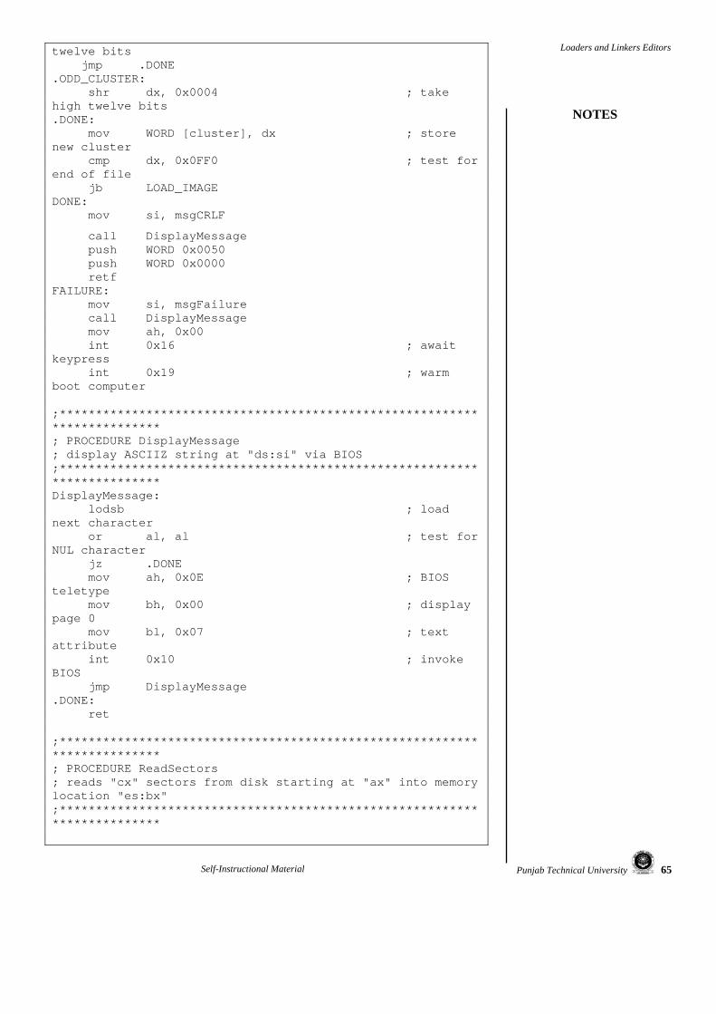
Punjab Technical University 65
Loaders and Linkers Editors
NOTES
Self-Instructional Material
twelve bits jmp .DONE .ODD_CLUSTER: shr dx, 0x0004 ; take high twelve bits .DONE: mov WORD [cluster], dx ; store new cluster cmp dx, 0x0FF0 ; test for end of file jb LOAD_IMAGE DONE: mov si, msgCRLF
call DisplayMessage push WORD 0x0050 push WORD 0x0000 retf FAILURE: mov si, msgFailure call DisplayMessage mov ah, 0x00 int 0x16 ; await keypress int 0x19 ; warm boot computer ;************************************************************************* ; PROCEDURE DisplayMessage ; display ASCIIZ string at "ds:si" via BIOS ;************************************************************************* DisplayMessage: lodsb ; load next character or al, al ; test for NUL character jz .DONE mov ah, 0x0E ; BIOS teletype mov bh, 0x00 ; display page 0 mov bl, 0x07 ; text attribute int 0x10 ; invoke BIOS jmp DisplayMessage .DONE: ret ;************************************************************************* ; PROCEDURE ReadSectors ; reads "cx" sectors from disk starting at "ax" into memory location "es:bx" ;*************************************************************************
66 Punjab Technical University
System Software
NOTES
Self-Instructional Material
ReadSectors: .MAIN mov di, 0x0005 ; five retries for error .SECTORLOOP push ax push bx push cx call LBACHS mov ah, 0x02 ; BIOS read sector mov al, 0x01 ; read one sector mov ch, BYTE [absoluteTrack] ; track mov cl, BYTE [absoluteSector] ; sector
mov dh, BYTE [absoluteHead] ; head mov dl, BYTE [DriveNumber] ; drive int 0x13 ; invoke BIOS jnc .SUCCESS ; test for read error xor ax, ax ; BIOS reset disk int 0x13 ; invoke BIOS dec di ; decrement error counter pop cx pop bx pop ax jnz .SECTORLOOP ; attempt to read again int 0x18 .SUCCESS mov si, msgProgress call DisplayMessage pop cx pop bx pop ax add bx, WORD [BytesPerSector] ; queue next buffer inc ax ; queue next sector loop .MAIN ; read next sector ret ;************************************************************************* ; PROCEDURE ClusterLBA ; convert FAT cluster into LBA addressing scheme ; LBA = (cluster - 2) * sectors per cluster ;************************************************************************* ClusterLBA: sub ax, 0x0002 ; zero base cluster number
Check Your Progress 4. Which FAT system is
specified for floppy disks? 5. What is the extension used for
library files? 6. To execute a program, what
do you need to use? A. DLL file B. EXE file C. LIB file D. DAS file

Punjab Technical University 67
Loaders and Linkers Editors
NOTES
Self-Instructional Material
xor cx, cx mov cl, BYTE [SectorsPerCluster] ; convert byte to word mul cx add ax, WORD [datasector] ; base data sector ret ;************************************************************************* ; PROCEDURE LBACHS ; convert "ax�2; LBA addressing scheme to CHS addressing scheme ; absolute sector = (logical sector / sectors per track) + 1 ; absolute head = (logical sector / sectors per track) MOD number of heads
; absolute track = logical sector / (sectors per track * number of heads) ;************************************************************************* LBACHS: xor dx, dx ; prepare dx:ax for operation div WORD [SectorsPerTrack] ; calculate inc dl ; adjust for sector 0 mov BYTE [absoluteSector], dl xor dx, dx ; prepare dx:ax for operation div WORD [NumHeads] ; calculate mov BYTE [absoluteHead], dl mov BYTE [absoluteTrack], al ret absoluteSector db 0x00 absoluteHead db 0x00 absoluteTrack db 0x00 datasector dw 0x0000 cluster dw 0x0000 ImageName db "LOADER BIN" msgLoading db 0x0D, 0x0A, "Loading Boot Image ", 0x0D, 0x0A, 0x00 msgCRLF db 0x0D, 0x0A, 0x00 msgProgress db ".", 0x00 msgFailure db 0x0D, 0x0A, "ERROR : Press Any Key to Reboot", 0x00 TIMES 510-($-$$) DB 0 DW 0xAA55 ;*************************************************************************

68 Punjab Technical University
System Software
NOTES
Self-Instructional Material
4.8 SUMMARY
The use of loaders and linkers in the operating system helps save memory space and speed up the execution of the program. Loaders and linkers helps you to have a schematic flow of steps to create a program. For performing a successful execution of a program you need to use a translator, loader and a linker. The design of a linker describes the relocation of addresses and linking of these addresses. But before you link all the object modules of a program, the booting of the computer is necessary, which is performed using a bootstrap loader. 4.9 ANSWERS TO ‘CHECK YOUR PROGRESS’
1. Many at a time
2. no
3. namelist[i], where i is a variable
4. FAT12
5. .lib
6. EXE file 4.10 EXERCISES AND QUESTIONS
Short-Answer Type Questions 1. What is the purpose of performing relocation ?
2. Explain the second pass of program linking.
3. What is the use of SEGTAB?
Long-Answer Type Questions 1. Explain the general loader scheme.
2. Name some library files used in system programming. 4.11 FURTHER READING
Dhamdhere, D. M., Systems Programming and Operating Systems.
Donovan, John J., Systems Programming, Tata McGraw-Hill Edition.

Punjab Technical University 69
Other System Softwares
NOTES
Self-Instructional Material
UNIT 5 OTHER SYSTEM SOFTWARES
Structure 5.0 Introduction 5.1 Unit Objectives 5.2 Operating System 5.3 Types of Operating Systems
5.3.1 Multiprocessing Operating System; 5.3.2 Multitasking; 5.3.3 Multi-user; 5.3.4 Multithreading; 5.3.5 Real-time Operating System
5.4 Functions of Operating System 5.4.1 Process Management; 5.4.2 Memory and Storage Management; 5.4.3 Protection and Security
5.5 DataBase Management System (DBMS) 5.5.1 Data; 5.5.2 Hardware; 5.5.3 Software; 5.5.4 End Users
5.6 Entities and Relationships 5.7 Functions and Structure of Text Editor 5.8 Summary 5.9 Answers to ‘Check your Progress’ 5.10 Exercises and Questions 5.11 Further Reading
5.0 INTRODUCTION
There are two types of computer softwares, application software and system software. Application softwares are the programs that help perform a specific task according to the utilisation of computer, such as managing the records of employees in a company. The examples of application software are spreadsheets, database systems and games. System software is a program that provides an interface to run application softwares and is less noticed by end users. The examples of system softwares are operating system and microprocessors. 5.1 UNIT OBJECTIVES
• Understanding the relationship between application software and system software
• Discussing various types of operating systems and their behaviour • Understanding the features of an operating system that helps provide security
and memory management • Introducing database management system and its application • Understanding the concept of Entity Relationship (ER) diagrams
5.2 OPERATING SYSTEM
An operating system is the system software that provides a communication medium between computer hardware and application software that user runs on a computer. An operating system helps manage connectivity between software and hardware of a
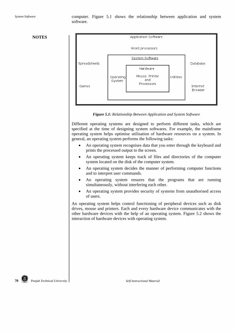
70 Punjab Technical University
System Software
NOTES
Self-Instructional Material
computer. Figure 5.1 shows the relationship between application and system software.
Figure 5.1: Relationship Between Application and System Software
Different operating systems are designed to perform different tasks, which are specified at the time of designing system softwares. For example, the mainframe operating system helps optimise utilisation of hardware resources on a system. In general, an operating system performs the following tasks:
• An operating system recognises data that you enter through the keyboard and prints the processed output to the screen.
• An operating system keeps track of files and directories of the computer system located on the disk of the computer system.
• An operating system decides the manner of performing computer functions and to interpret user commands.
• An operating system ensures that the programs that are running simultaneously, without interfering each other.
• An operating system provides security of systems from unauthorised access of users.
An operating system helps control functioning of peripheral devices such as disk drives, mouse and printers. Each and every hardware device communicates with the other hardware devices with the help of an operating system. Figure 5.2 shows the interaction of hardware devices with operating system.

Punjab Technical University 71
Other System Softwares
NOTES
Self-Instructional Material
Figure 5.2: Interaction of Hardware Devices with Operating System
5.3 TYPES OF OPERATING SYSTEMS
A computer system is useless if you do not install an operating system on it. You can install any operating system on a computer system according to the requirement of the end user. There are following types of operating systems:
• Multiprocessing • Multitasking • Multi-user • Multithreading • Real time
5.3.1 Multiprocessing Operating System Multiprocessing operating system such as Linux, Unix and Windows 2000 allows you to run a single program on more than one CPU. Multiprocessing operating systems are of two types, shared memory and distributed memory. In shared memory multiprocessing operating system, all CPU share same memory and can communicate easily with each other. In the distributed multiprocessing operating system, all CPU have separate memory that slows the processing speed of CPU.
5.3.2 Multitasking Multitasking is the ability of an operating system to manage several applications at a time. The operating system processor assign a time slot to each program that is running on the operating system for the execution of the application. This allotment of time to the programs allows you to share the devices and memory of a multitasking operating system. Multitasking can be implemented in two ways:
• Co-operative multitasking • Pre-emptive multitasking
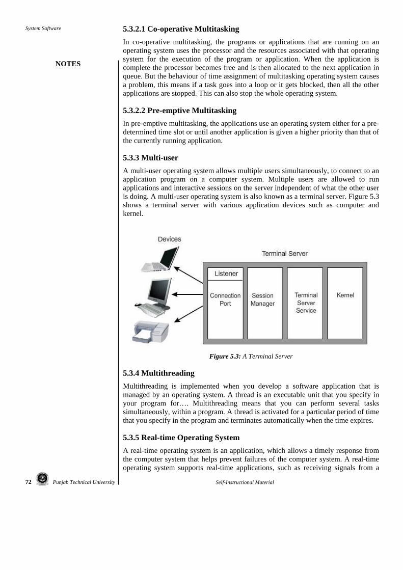
72 Punjab Technical University
System Software
NOTES
Self-Instructional Material
5.3.2.1 Co-operative Multitasking In co-operative multitasking, the programs or applications that are running on an operating system uses the processor and the resources associated with that operating system for the execution of the program or application. When the application is complete the processor becomes free and is then allocated to the next application in queue. But the behaviour of time assignment of multitasking operating system causes a problem, this means if a task goes into a loop or it gets blocked, then all the other applications are stopped. This can also stop the whole operating system.
5.3.2.2 Pre-emptive Multitasking In pre-emptive multitasking, the applications use an operating system either for a pre-determined time slot or until another application is given a higher priority than that of the currently running application.
5.3.3 Multi-user A multi-user operating system allows multiple users simultaneously, to connect to an application program on a computer system. Multiple users are allowed to run applications and interactive sessions on the server independent of what the other user is doing. A multi-user operating system is also known as a terminal server. Figure 5.3 shows a terminal server with various application devices such as computer and kernel.
Figure 5.3: A Terminal Server
5.3.4 Multithreading Multithreading is implemented when you develop a software application that is managed by an operating system. A thread is an executable unit that you specify in your program for…. Multithreading means that you can perform several tasks simultaneously, within a program. A thread is activated for a particular period of time that you specify in the program and terminates automatically when the time expires.
5.3.5 Real-time Operating System A real-time operating system is an application, which allows a timely response from the computer system that helps prevent failures of the computer system. A real-time operating system supports real-time applications, such as receiving signals from a

Punjab Technical University 73
Other System Softwares
NOTES
Self-Instructional Material
satellite and allows the execution of a program at the time when you receive the signals from the satellite. The behaviour of a real-time application allows you to analyse the response time of an application. For example, a satellite sends digitised samples of receiving data at the rate of 5000 samples per second. The application program on an operating system stores these samples in a file. Since every millisecond a new sample arrives, the application program is required to respond to each request to store the data. Failure in storing the data results in the loss of data. Figure 5.4 shows a satellite system that is a real-time application and receives data from a satellite and stores the data in a file located on the operating system.
Figure 5.4: Real-Time Application
5.4 FUNCTIONS OF OPERATING SYSTEM
The main function of an operating system is to manage the computer system resources. An operating system allows you to keep track of all the resources used by an end user, to grant and block a resource request of an end user. When multiple users use a computer, you need to manage and protect the memory and input and output devices. The various functions provided by an operating system are:
• Process Management • Memory and Storage Management • Protection and Security
5.4.1 Process Management A process management ensures that each application and process receives enough time of the processor to execute a process, which helps operating system to function properly and make real-time application work possible. The basic unit of a software in an operating system is a process. A process is software that performs some action, which an end user controls by using other applications or by using an operating
Check Your Progress 1. What is a kernel? 2. Which operating system do
you prefer in a Linux lab? 3. When you connect a computer
to the Internet, which operating system is used?

74 Punjab Technical University
System Software
NOTES
Self-Instructional Material
system. A process controls and schedules the execution of a program. The structure of a process includes:
• A process stack, which contains temporary data such as function parameters, return addresses and local variables.
• A data section, which contains global variables. • A heap, which is memory that is dynamically loaded during run time.
Figure 5.5 shows the structure of a process that specifies process management.
Figure 5.5: Process in Memory
As a process executes, it changes state from one state to another when you receive an instruction. The state is defined as the current activity of a process, which is executed by the processor. Figure 5.6 shows various states that a process can attain.
Figure 5.6: Process State

Punjab Technical University 75
Other System Softwares
NOTES
Self-Instructional Material
5.4.2 Memory and Storage Management Memory management allows an operating system to use the available memory of a computer system effectively. Memory management ensures that each process is allocated with enough memory space for properly executing it. An operating system set up memory boundaries for each type of software and individual applications. The different types of memory used in a computer system are:
• High speed cache: Cache is a very fast memory, which is available to CPU in small amount. CPU controller helps predict the next piece of data in queue, which is allocated the cache memory to complete a task. A cache memory improves the performance of a computer system.
• Main memory: RAM is referred as the main memory of a computer system. • Secondary memory: Secondary memory stores the data on magnetic tapes
and keeps the data and application available to the end user.
5.4.3 Protection and Security Computer systems contain many objects that you need to protect from misuse by the end users. These objects can be hardware objects such as memory, CPU time and input and output devices or software objects such as files and programs. An operating system imposes a protection policy on computer system resources or on its end users. It also provides mechanisms that enable privileges such as using only specified applications of an operating system for maintaining the security of the computer system when they are needed and disable them when they are not needed. 5.5 DATABASE MANAGEMENT SYSTEM (DBMS)
DataBase Management System (DBMS) is a system that maintains computerised record or data on a computer system. The main purpose of DBMS is to store information and to allow end users to retrieve data from the database located on the operating system. The information stored in DBMS can be related to an individual or to an organisation. Figure 5.7 shows a database system that contains four major components: data, hardware, software and end users that can use database system.
Figure 5.7: A Database System
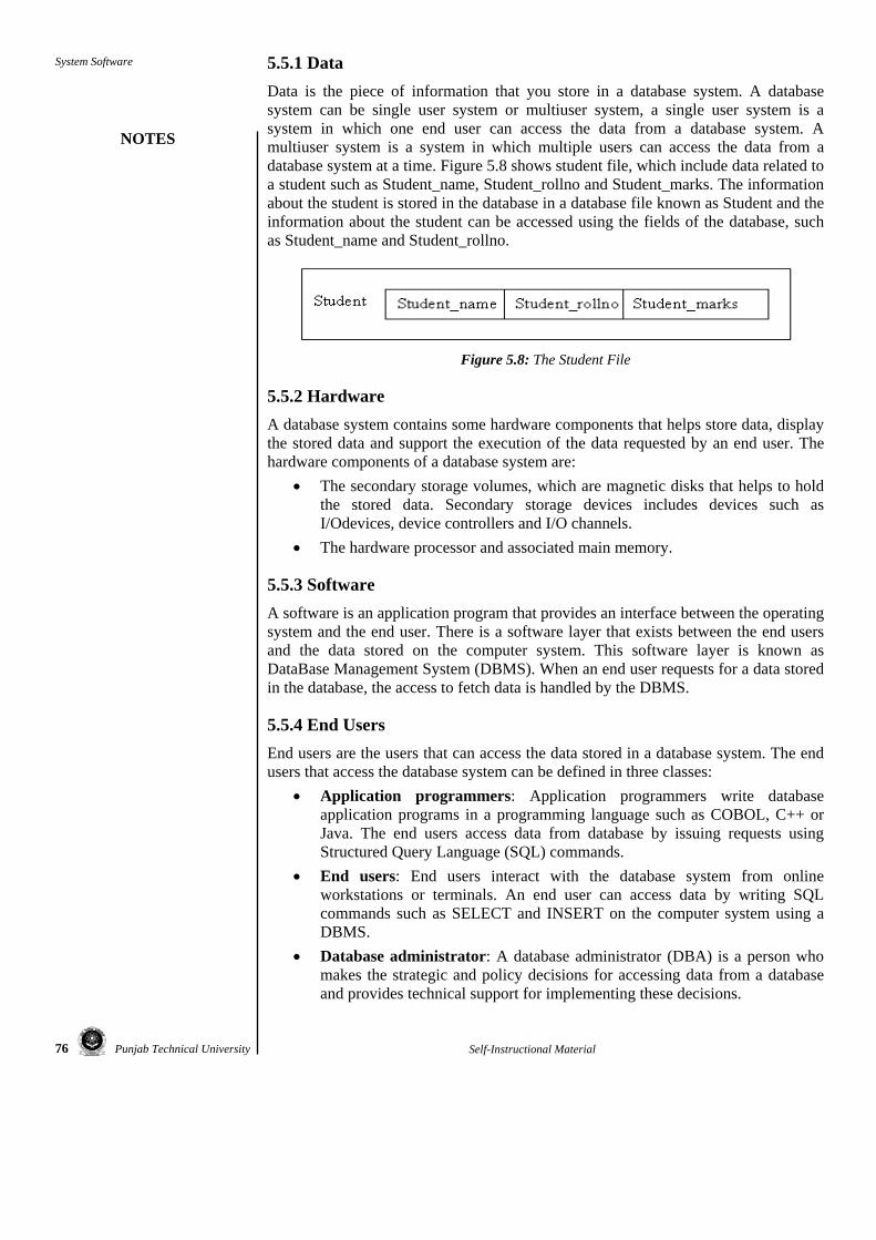
76 Punjab Technical University
System Software
NOTES
Self-Instructional Material
5.5.1 Data Data is the piece of information that you store in a database system. A database system can be single user system or multiuser system, a single user system is a system in which one end user can access the data from a database system. A multiuser system is a system in which multiple users can access the data from a database system at a time. Figure 5.8 shows student file, which include data related to a student such as Student_name, Student_rollno and Student_marks. The information about the student is stored in the database in a database file known as Student and the information about the student can be accessed using the fields of the database, such as Student_name and Student_rollno.
Figure 5.8: The Student File
5.5.2 Hardware A database system contains some hardware components that helps store data, display the stored data and support the execution of the data requested by an end user. The hardware components of a database system are:
• The secondary storage volumes, which are magnetic disks that helps to hold the stored data. Secondary storage devices includes devices such as I/Odevices, device controllers and I/O channels.
• The hardware processor and associated main memory.
5.5.3 Software A software is an application program that provides an interface between the operating system and the end user. There is a software layer that exists between the end users and the data stored on the computer system. This software layer is known as DataBase Management System (DBMS). When an end user requests for a data stored in the database, the access to fetch data is handled by the DBMS.
5.5.4 End Users End users are the users that can access the data stored in a database system. The end users that access the database system can be defined in three classes:
• Application programmers: Application programmers write database application programs in a programming language such as COBOL, C++ or Java. The end users access data from database by issuing requests using Structured Query Language (SQL) commands.
• End users: End users interact with the database system from online workstations or terminals. An end user can access data by writing SQL commands such as SELECT and INSERT on the computer system using a DBMS.
• Database administrator: A database administrator (DBA) is a person who makes the strategic and policy decisions for accessing data from a database and provides technical support for implementing these decisions.

Punjab Technical University 77
Other System Softwares
NOTES
Self-Instructional Material
5.6 ENTITIES AND RELATIONSHIPS
Entity is an object that helps store data and specifies relationship between different entities of DBMS. You need to understand the entities and relationships with the help of diagrams. The Entity Relationship Diagrams (ERD) helps specify the logical structure of a database and inter-relationships between entities of a database. ER diagrams use symbols to represent information such as diamonds, boxes and ovals. Table 5.1 shows various symbols that you can use in ER diagram to represent information.
Table 5.1: Various Symbols Used in ER Diagram
Symbol Meaning
Entity
Weak Entity
Relationship
Identity Relationship
Attribute
Key attribute
Multivalued
Composite Attribute
Derived Attribute
Total participation of E2 In R
Cardinality Ratio 1:N For E1:E2 In R, where E1 and E2 are the entities and R is the relationship between the entities E1 and E2
Check Your Progress 4. What is the basic unit of
software in an operating system?
5. Who grants permission to an end user for accessing data?
6. Name the text editor for Microsoft?

78 Punjab Technical University
System Software
NOTES
Self-Instructional Material
5.7 FUNCTIONS AND STRUCTURE OF TEXT EDITOR
A text editor is an interactive program that allows you to input, delete, update and store information on a computer system such as data, programs and letters. The data and information in a computer system are stored in a simple format referred as plain text. The text is stored in the memory in some memory units, this memory unit is known as byte. One byte that includes eight bits of data represents a character of text in a plain text file. The examples of applications that include plain text are e-mail messages and various Hyper Text Mark-Up Language (HTML) Web pages.
A text editor is a program that creates and modifies the text files. The application of text editor can be seen in the following areas:
• Writing e-mails • Composing Web pages • Creating computer programs • Installing files that control the text files
5.8 SUMMARY
An operating system is the interface that helps build a platform between a computer’s hardware and the software applications. The heart of an operating system is a kernel that helps pass commands system given by the end users to an operating system. The database management system helps access data stored on the database and allows you to update, delete or store data using SQL commands. A database maintains many entities, which are the objects that store data on the computer system. ER diagrams help specify a relationship between the different entities. A text editor is an interactive software program that helps in writing a text. 5.9 ANSWERS TO ‘CHECK YOUR PROGRESS’
1. Kernel is a piece of software, which is a fundamental part of an operating system that provides a secure access to hardware of a computer system.
2. Multi-user
3. Real-time operating system
4. Process
5. DBA
6. Notepad 5.10 EXERCISES AND QUESTIONS
Short-Answer Questions 1. What is an operating system?
2. How does pre-emptive multitasking uses CPU?

Punjab Technical University 79
Other System Softwares
NOTES
Self-Instructional Material
3. What are the drawbacks of a real-time operating system?
4. What are the different types of operating system?
Long-Answer Questions 1. What are SQL commands?
2. How does ER diagram help in removing the complexity of a database? 5.11 FURTHER READING
Date, C. J., An Introduction to Database Systems.
Galvin, Operating System Principles.

PUNJAB TECHNICAL UNIVERSITY LADOWALI ROAD, JALANDHAR
INTERNAL ASSIGNMENT
TOTAL MARKS: 25
NOTE: Attempt any 5 questions All questions carry 5 Marks. Q. 1. What are the steps involved in the design procedure of an assembler? Q. 2. Explain the difference between a directive, an operation and an instruction. Give an
example of each. Q. 3. Give an example to show the implementation of an assembly language program. Q. 4. Explain two-pass macro pre-processor in detail. Q. 5. Explain the following in detail: A. Macro expansion B. Conditional macro expansion Q. 6. Draw a parse tree for the expression 3– 4 * 4 + 2 Q. 7. Why were compilers introduced? Q. 8. If compilers helps in compiling a file, then what does loader and linker do? Q. 9. How will you recognise a weak entity in ER diagram? Q.10. How can you fetch data from a database using SQL commands?

PUNJAB TECHNICAL UNIVERSITY LADOWALI ROAD, JALANDHAR
ASSIGNMENT SHEET
(To be attached with each Assignment) ________________________________________________________________________
Full Name of Student:_____________________________________________________________ (First Name) (Last Name) Registration Number:
Course:__________ Sem.:________ Subject of Assignment:________________________________ Date of Submission of Assignment:
(Question Response Record-To be completed by student)
Total Marks:_____________/25
Remarks by Evaluator:__________________________________________________________________ __________________________________________________________________________________ Note: Please ensure that your Correct Registration Number is mentioned on the Assignment Sheet. Name of the Evaluator Signature of the Student Signature of the Evaluator Date:_______________ Date:_______________
S.No. Question Number Responded
Pages ____ - ____ of Assignment
Marks
1 2 3 4 5 6 7 8 9
10