System Integration Schedule Estimating Relationships (SERs)

NASA Cost and Schedule Symposium

August 13-15, 2019 • Houston, TX

System Integration Schedule Estimating Relationships (SERs)

Presented by:

Marc GreenbergStrategic Investment Division (SID)

National Aeronautics and Space Administration

Outline

• Task Objectives

• Background

• Schedule Data from SMART

• Methodology

– Equation 1: Y = 0.3617 X -0.568

– Equations 2a, 2b, 3a and 3b

– “Knee in the Curve” for Equation 1

• Example for notional project

– Apply equations 2a, 2b, 3a and 3b

– Sensitivity analysis

• Conclusions and Future Work

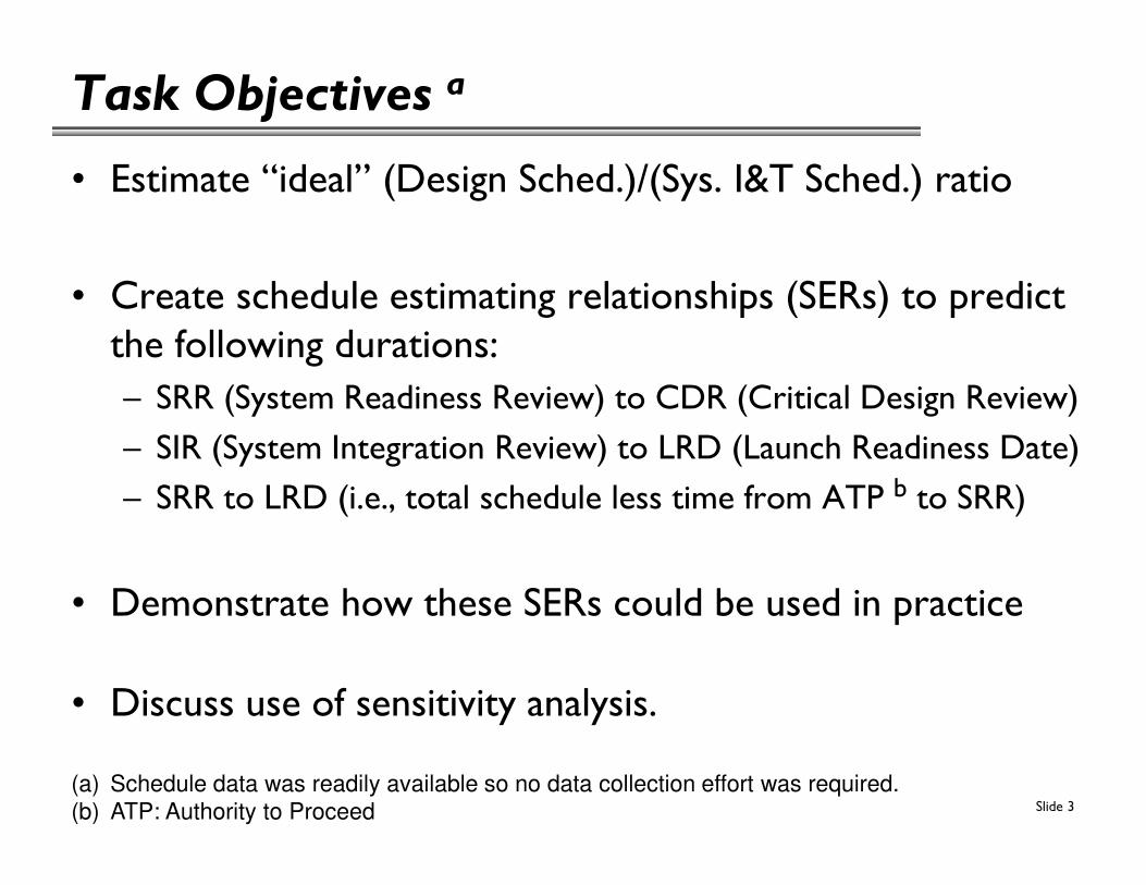
Task Objectives a

• Estimate “ideal” (Design Sched.)/(Sys. I&T Sched.) ratio

• Create schedule estimating relationships (SERs) to predict the following durations:

– SRR (System Readiness Review) to CDR (Critical Design Review)

– SIR (System Integration Review) to LRD (Launch Readiness Date)

– SRR to LRD (i.e., total schedule less time from ATP to SRR)

• Demonstrate how these SERs could be used in practice

• Discuss use of sensitivity analysis.

b

(a) Schedule data was readily available so no data collection effort was required.

ATP: Authority to Proceed(b)

Background: Milestones from SRR to LRDPhase A-B

System LevelDesign Requirements

Item LevelDesign Requirements

SRR

PDR

Phase C

All Design Requirements Complete

CDR

Phase D-E

System Level

Subsystems

Element

Component

LRD

SIR

Major Milestones: SRR: Systems Readiness Review

PDR: Preliminary Design Review

CDR: Critical Design Review

SIR: System Integration Review

LRD: Launch Readiness Date

Schedule Data from SMART

NASA’s Schedule Management and Relationship Tool (SMART) provided schedule data from 55 science missions. Values in Months. Mission SRR-PDR PDR-CDR CDR-SIR SIR-LRD SRR-LRD

CONTOUR 8 11 14 5 38

Dawn 6 8 7 33 54

Deep Impact 10 11 16 20 57

Deep Space 1 3 9 11 15 38

Galileo 9 33 15 82 139

InSight 28 9 9 39 85

Juno 30 11 12 16 69

MAP 8 5 35 14 62

MAVEN 11 12 12 17 52

MER-A 3 14 3 16 36

MER-B 3 14 4 15 36

MESSENGER 13 10 10 19 52

MRO 6 10 11 16 43

MSL 6 12 9 46 73

OSIRIS-REX 10 13 11 19 53

Phoenix 11 8 5 16 40

Stardust 6 9 7 13 35

Chandra X-Ray 23 15 20 22 80

COBE 15 25 35 15 90

FGST (GLAST) 33 15 23 22 93

GALEX 3 8 26 20 57

IBEX 4 8 13 13 38

Kepler 12 24 19 10 65

RHESSI 7 4 13 26 50

SAMPEX 3 10 14 11 38

SDO 11 13 0 59 83

Spitzer 7 12 41 19 79

STEREO 19 14 18 26 77

Mission SRR-PDR PDR-CDR CDR-SIR SIR-LRD SRR-LRD

SWAS 31 10 10 52 103

WIRE 23 0 17 18 58

WISE 7 23 17 13 60

NuSTAR 11 8 12 17 48

OCO 12 25 20 11 68

ACE 12 12 19 16 59

ACTS 10 24 37 27 98

AIM 8 10 0 30 48

Aqua 5 14 1 47 67

Aura 5 14 13 34 66

Calipso 8 18 11 26 63

CHIPSAT 12 8 14 8 42

DART 5 4 7 25 41

EO-1 8 10 5 21 44

FAST 14 10 15 33 72

Glory 12 11 19 38 80

IMAGE 9 5 20 12 46

IRIS 3 7 18 13 41

LANDSAT-7 12 13 16 27 68

LANDSAT-8 14 10 18 14 56

NPP 35 9 62 36 142

OSTM/Jason-2 10 44 7 12 73

Aquarius 12 36 11 25 84

MMS 20 13 25 31 89

SMAP 22 9 9 22 62

TRACE 2 1 16 13 32

VABP (RBSP) 8 14 11 23 56

Methodology: Equation 1: Y = 0.3617 X -0.568

Relative Sys I&T Schedule vs. "Design-to-Sys I&T" Schedule Ratio(SIR to LRD / SRR to LRD) versus (SRR to CDR / SIR to LRD)

0.00

0.10

0.20

0.30

0.40

0.50

0.60

0.70

0.80

0.90

0.00 0.50 1.00 1.50 2.00 2.50 3.00 3.50 4.00 4.50 5.00

Sy

s I&

T S

che

du

le a

s %

of

Pro

ject

Sch

ed

ule

= (

SIR

to

LR

D )

/ (

SR

R t

o L

RD

)

Design Schedule relative to Sys I&T Schedule = (SRR to CDR) / (SIR to LRD)

Potentially insufficient design schedule

As (SRR to CDR) / (SIR to LRD) increases, (SIR to LRD) / (SRR to LRD) decreases.

i.e., As relative design schedule increases, relative sys I&T schedule decreases.

Y: (SIR to CDR)(SRR to LRD)

~ Sys I&T vs. Total Sched.

X: (SRR to CDR)(SIR to LRD)

~ Design vs. Sys I&T

Y = 0.3617 X -0.568

R2 = 0.79 (MUPE)

Methodology: Equations 2a, 2b, 3a and 3b

Note: Schedule data in Months; Sample size = 55

Eq. 2a: SRR to CDR = 0.3060 * SRR to LRD 1.041 Design vs Sys I&T 0.4306

(SRR to CDR)(SIR to LRD)

Adj-R2 (MUPE) = 0.86; Avg. = 24.5 mo. SE = 4.3 mo.; MAD = 13.4%

Rearrange Equation 2a to create Equation 2b …

Eq. 2b: SRR to LRD = 3.1196 * SRR to CDR 0.9607 Design vs Sys I&T -0.4137

Eq. 3a: SIR to LRD = 0.3060 * SRR to LRD 1.041 Design vs Sys I&T -0.5694

Adj-R2 (MUPE) = 0.91; Avg. = 23.4 mo. SE = 4.5 mo.; MAD = 13.4%

Rearrange Equation 3a to create Equation 3b …

Eq. 3b: SRR to LRD = 3.1196 * SIR to LRD 0.9607 Design vs Sys I&T 0.5470

Q: How can we use each SER if we must know not one but up to three independent variables? A: Simplify “Design vs Sys I&T” input!

Methodology: “Knee in the Curve” for Eq. 1

Relative Sys I&T Schedule vs. "Design-to-Sys I&T" Schedule Ratio(SIR to LRD / SRR to LRD) versus (SRR to CDR / SIR to LRD)

0.00

0.10

0.20

0.30

0.40

0.50

0.60

0.70

0.80

0.90

0.00 0.50 1.00 1.50 2.00 2.50 3.00 3.50 4.00 4.50 5.00

Sy

s I&

T S

che

du

le a

s %

of

Pro

ject

Sch

ed

ule

= (

SIR

to

LR

D )

/ (

SR

R t

o L

RD

)

Design Schedule relative to Sys I&T Schedule = (SRR to CDR) / (SIR to LRD)X= 1.175

Knee in the curve: Point on curve where distance

between line & curve is greatest. Must find the

point tangent to curve parallel to straight line.

1. Connect endpoints of Y = 0.3617 X -0.568

2. Calculate Slope of straight line = -0.159

3. Derivative of Y = 0.3617 X -0.568

= Straight line = -0.2055 X -1.568

4. Given Y’ = -0.2055 X -1.568 … find X where slope = -0.159

Methodology: “Knee in the Curve” for Eq. 1Calculation of "Knee in the Curve" for:

Relative Sys I&T Schedule vs. "Design-to-Sys I&T" Schedule Ratio

X = 1.175

Y = 0.330

0.00

0.10

0.20

0.30

0.40

0.50

0.60

0.70

0.80

0.90

0.00 0.50 1.00 1.50 2.00 2.50 3.00 3.50 4.00 4.50 5.00

Sys

I&T

Sch

ed

ule

as

% o

f P

roje

ct S

che

du

le =

(S

IR t

o L

RD

) /

(SR

R t

o L

RD

)

Design Schedule relative to Sys I&T Schedule = (SRR to CDR) / (SIR to LRD)

Knee in the curve: That point on the curve

where distance between the “connector”

line and curve is greatest … … that point on the curve is (1.175, 0.330)

X = “Design vs Sys I&T” = 1.175

“Design vs. Sys I&T” = (SRR to CDR)(SIR to LRD)

For all SERs, we assume an “ideal” Design vs Sys I&T

input = 1.175

y = 0.3617x-0.568

Example for Notional Project: Equation 2a

Eq. 2a: SRR to CDR = 0.3060 * SRR to LRD 1.041 Design vs Sys I&T 0.4306

• Input 1: SRR to LRD = 60 mos. (e.g., constraint for planetary mission “M”)

• Input 2: Design vs Sys I&T = 1.175 (“knee-in-the-curve” value)

SRR to CDR = 0.3060 * 60 1.041 1.175 0.4306 = 23.3 mos.

1.175 = SRR to CDR SIR to LRD

so … SIR to LRD = 23.31.175

= 19.8 mos.

CDR to SIR = (SRR to LRD) – (SRR to CDR) – (SIR to LRD) = 16.9 mos. 60 23.3 19.8

SRR to CDR = 23.3 CDR to SIR = 16.9 SIR to LRD = 19.8

0 10 20 30 40 50 60

Estimates of "SRR to CDR", "CDR to SIR" and "SIR to LRD" (in months)

SRR to LRD (Given) = 60 months

39% 28% 33%

We can now rearrange Eq. 2a to form Eq. 2b

where Y = SRR to LRD.

Example for Notional Project: Equation 2b

Eq. 2b: SRR to LRD = 3.1196 * SRR to CDR 0.9607 Design vs Sys I&T -0.4137

• Input 1: SRR to CDR = 23.3 mos. (e.g., in-family for planetary mission “M”)


SRR to LRD = 3.1196 * 23.3 0.9607 1.175 -0.4137 = 60.0 mos.


so … SIR to LRD = 23.31.175

= 19.8 mos.



0 10 20 30 40 50 60

Estimates of "CDR to SIR" , "SIR to LRD" and "SRR to LRD" (in months)

(Given)

SRR to LRD (estim) = 60

39% 28% 33%

Example for Notional Project: Equation 3a

Eq. 3a: SIR to LRD = 0.3060 * SRR to LRD 1.041 Design vs Sys I&T -0.5694

• Input 1: SRR to LRD = 60 mos. (e.g., constraint for planetary mission “M”)


SIR to LRD = 0.3060 * 60 1.041 1.175 -0.5694 = 19.8 mos.


so … SRR to CDR = 1.175 * 19.8 = 23.3 mos.



0 10 20 30 40 50 60

Estimates of "SRR to CDR", "CDR to SIR" and "SIR to LRD" (in months)

SRR to LRD (Given) = 60 months

39% 28% 33%

We can now rearrange Eq. 3a to form Eq. 3b

where Y = SRR to LRD.

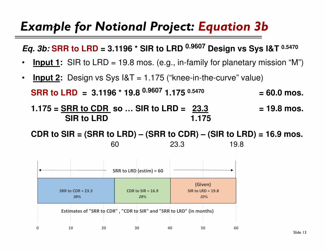
Example for Notional Project: Equation 3b

Eq. 3b: SRR to LRD = 3.1196 * SIR to LRD 0.9607 Design vs Sys I&T 0.5470

• Input 1: SIR to LRD = 19.8 mos. (e.g., in-family for planetary mission “M”)


SRR to LRD = 3.1196 * 19.8 0.9607 1.175 0.5470 = 60.0 mos.


so … SIR to LRD = 23.31.175

= 19.8 mos.



0 10 20 30 40 50 60

Estimates of "SRR to CDR" , "CDR to SIR" and "SRR to LRD" (in months)

(Given)

SRR to LRD (estim) = 60

39% 28% 33%

Example for Notional Project: Sensitivity Analysis

It’s important to explore how changing SER inputs can impact schedule estimates …

1.175

60

Equation 2a: Estimate SRR to CDR Input 1: SRR to LRD (months)

23.3 40 45 50 55 60 65 70 75 80

1.025 14.4 16.3 18.1 20.0 21.9 23.8 25.8 27.7 29.6

1.100 14.8 16.8 18.7 20.7 22.6 24.6 26.6 28.5 30.5

1.175 15.3 17.2 19.2 21.3 23.3 25.3 27.3 29.4 31.4

1.250 15.7 17.7 19.8 21.8 23.9 26.0 28.1 30.1 32.2

1.325 16.1 18.2 20.3 22.4 24.5 26.6 28.8 30.9 33.1

Input 2: Design vs Sys I&T

1.175

23.3

Equation 2b: Estimate SRR to LRD Input 1: SRR to CDR (months)

60.0 9 12 15 18 23.3 27 30 33 36

1.025 25.5 33.6 41.6 49.6 63.5 73.2 81.0 88.8 96.6

1.100 24.8 32.6 40.4 48.2 61.7 71.1 78.7 86.3 93.8

1.175 24.1 31.8 39.4 46.9 60.0 69.2 76.6 83.9 91.2

1.250 23.5 31.0 38.4 45.7 58.5 67.5 74.7 81.8 88.9

1.325 22.9 30.2 37.4 44.6 57.1 65.9 72.9 79.9 86.8


Example: Given SRR to CDR = 23.3 mos., if Design v Sys I&T changed from 1.175 to 1.025, then SRR to LRD would increase to 63.5 mos.

Example for Notional Project: Sensitivity Analysis

It’s important to explore how changing SER inputs can impact schedule estimates …

1.175

60

Equation 3a: Estimate SIR to LRD Input 1: SRR to LRD (months)

19.8 40 45 50 55 60 65 70 75 80

1.025 14.0 15.9 17.7 19.6 21.4 23.3 25.1 27.0 28.9

1.100 13.5 15.2 17.0 18.8 20.6 22.3 24.1 25.9 27.7

1.175 13.0 14.7 16.4 18.1 19.8 21.5 23.2 25.0 26.7

1.250 12.5 14.2 15.8 17.5 19.1 20.8 22.4 24.1 25.8

1.325 12.1 13.7 15.3 16.9 18.5 20.1 21.7 23.3 25.0


1.175

19.80

Equation 3b: Estimate SRR to LRD Input 1: SIR to LRD (months)

60.0 6 9 12 18 19.8 24 27 30 33

1.025 17.7 26.1 34.4 50.8 55.7 67.0 75.0 83.0 90.9

1.100 18.4 27.1 35.8 52.8 57.9 69.6 78.0 86.3 94.5

1.175 19.1 28.1 37.1 54.7 60.0 72.2 80.8 89.4 98.0

1.250 19.7 29.1 38.4 56.6 62.1 74.7 83.6 92.5 101.4

1.325 20.3 30.0 39.6 58.5 64.1 77.1 86.3 95.5 104.7


Example: If SRR to LRD increased to 70 mos. and if Design v Sys I&Tdecreased to 1.025, then SIR to LRD increases from 19.8 to 25.1 mos.

Conclusions & Future Work

• Regression analysis of schedule data produced five SERs.

• Assumed a regime on the curve where an “ideal” amount of design schedule leads to an “ideal” system I&T schedule.

• Use of these SERs can assist estimators in bounding schedule durations from key milestone to key milestone.

– Example: Is the program’s SRR to CDR estimate in-family?

• Future work includes the following tasks:

– Revisit data. Use outlier analysis to learn more on unusual obs.

– Create approach to deviate from knee-in-the-curve (X = 1.175)

– Add pred. intervals to enable showing Y-values at any probability

– Where possible, add data where data is missing in SMART data.

– Where data is sufficient, conduct regressions to estimate …

• ATP to SRR, SRR to PDR, PDR to CDR and ATP to LRD.

System Integration Schedule Estimating Relationships (SERs)

Documents

Transcript of System Integration Schedule Estimating Relationships (SERs)