Symplectic Geometry and its Applicationsv1ranick/papers/arnogive.pdf · classical mechanics,...
69
Symplectic Geometry V. I. Arnol’d, A. B. Givental’ Translated from the Russian by G. Wassermann Contents Foreword. .............................................. 4 Chapter 1. Linear Symplectic Geometry ....................... 5 4 1. Symplectic Space ...................................... 5 1.1. The Skew-Scalar Product .............................. 5 1.2. Subspaces.. ........................................ 5 1.3. The Lagrangian Grassmann Manifold. .................... 6 4 2. Linear Hamiltonian Systems ............................. 7 2.1. The Symplectic Group and its Lie Algebra. ................ 7 2.2. The Complex Classification of Hamiltonians. ............... 8 2.3. Linear Variational Problems. ........................... 9 2.4. Normal Forms of Real Quadratic Hamiltonians. ............ 10 2.5. Sign-Definite Hamiltonians and the Minimax Principle ....... 11 $3. Families of Quadratic Hamiltonians ....................... 12 3.1. The Concept of the Miniversal Deformation. ............... 12 3.2. Miniversal Deformations of Quadratic Hamiltonians ......... 13 3.3. Generic Families ..................................... 14 3.4. Bifurcation Diagrams ................................. 16 94. The Symplectic Group. ................................. 17 4.1. The Spectrum of a Symplectic Transformation .............. 17 4.2. The Exponential Mapping and the Cayley Parametrization .... 18 4.3. Subgroups of the Symplectic Group ...................... 18 4.4. The Topology of the Symplectic Group ................... 19 4.5. Linear Hamiltonian Systems with Periodic Coefficients ....... 19
Transcript of Symplectic Geometry and its Applicationsv1ranick/papers/arnogive.pdf · classical mechanics,...

Symplectic Geometry
V. I. Arnol’d, A. B. Givental’
Translated from the Russian by G. Wassermann
Contents
Foreword. .............................................. 4
Chapter 1. Linear Symplectic Geometry ....................... 5
4 1. Symplectic Space ...................................... 5 1.1. The Skew-Scalar Product .............................. 5 1.2. Subspaces.. ........................................ 5 1.3. The Lagrangian Grassmann Manifold. .................... 6
4 2. Linear Hamiltonian Systems ............................. 7 2.1. The Symplectic Group and its Lie Algebra. ................ 7 2.2. The Complex Classification of Hamiltonians. ............... 8 2.3. Linear Variational Problems. ........................... 9 2.4. Normal Forms of Real Quadratic Hamiltonians. ............ 10 2.5. Sign-Definite Hamiltonians and the Minimax Principle ....... 11
$3. Families of Quadratic Hamiltonians ....................... 12 3.1. The Concept of the Miniversal Deformation. ............... 12 3.2. Miniversal Deformations of Quadratic Hamiltonians ......... 13 3.3. Generic Families ..................................... 14 3.4. Bifurcation Diagrams ................................. 16
94. The Symplectic Group. ................................. 17 4.1. The Spectrum of a Symplectic Transformation .............. 17 4.2. The Exponential Mapping and the Cayley Parametrization .... 18 4.3. Subgroups of the Symplectic Group ...................... 18 4.4. The Topology of the Symplectic Group ................... 19 4.5. Linear Hamiltonian Systems with Periodic Coefficients ....... 19

2 V.I. Arnol’d, A.B. Givental
Chapter 2. Symplectic Manifolds. ............................
4 1. Local Symplectic Geometry. .............................
1.1. The Darboux Theorem ................................
1.2. Example. The Degeneracies of Closed 2-Forms on [w4 ........ 1.3. Germs of Submanifolds of Symplectic Space. ............... 1.4. The Classification of Submanifold Germs .................. 1.5. The Exterior Geometry of Submanifolds. .................. 1.6. The Complex Case ...................................
$2. Examples of Symplectic Manifolds. ........................
2.1. Cotangent Bundles ................................... 2.2. Complex Projective Manifolds .......................... 2.3. Symplectic and KHhler Manifolds ........................
2.4. The Orbits of the Coadjoint Action of a Lie Group .......... 33. The Poisson Bracket ...................................
3.1. The Lie Algebra of Hamiltonian Functions. ................ 3.2. Poisson Manifolds. ...................................
3.3. Linear Poisson Structures .............................. 3.4. The Linearization Problem. ............................
0 4. Lagrangian Submanifolds and Fibrations ................... 4.1. Examples of Lagrangian Manifolds. ...................... 4.2. Lagrangian Fibrations. ................................
4.3. Intersections of Lagrangian Manifolds and Fixed Points of Symplectomorphisms. .................................
Chapter 3. Symplectic Geometry and Mechanics. ................
5 1. Variational Principles. .................................. 1.1. Lagrangian Mechanics. ................................ 1.2. Hamiltonian Mechanics. ............................... 1.3. The Principle of Least Action ...........................
1.4. Variational Problems with Higher Derivatives .............. 1.5. The Manifold of Characteristics .........................
1.6. The Shortest Way Around an Obstacle. ................... 6 2. Completely Integrable Systems. ...........................
2.1. Integrability According to Liouville. ...................... 2.2. The “Action-Angle” Variables ........................... 2.3. Elliptical Coordinates and Geodesics on an Ellipsoid. ........ 2.4. Poisson Pairs. .......................................
2.5. Functions in Involution on the Orbits of a Lie Coalgebra ..... 2.6. The Lax Representation ...............................
9 3. Hamiltonian Systems with Symmetries. ..................... 3.1. Poisson Actions and Momentum Mappings ................ 3.2. The Reduced Phase Space and Reduced Hamiltonians ........ 3.3. Hidden Symmetries ...................................
22
22 22 23 24 25 26 27 27 27 28 29 30 31 31 32 33 34 35 35 36
38
42
42 43 44 45 46 48 49 51 51 53 54 57 58 59 61 61 62 63
Symplectic Geometry
3.4. Poisson Groups. . . . . . . . . . . . . . . . . . . . . . . . . . . . . . . . 65 3.5. Geodesics of Left-Invariant Metrics and the Euler Equation . . 66 3.6. Relative Equilibria. . . . . . . . . . . . . . . . . . . . . . . . . . . . . . . . . . 66 3.7. Noncommutative Integrability of Hamiltonian Systems . . , . . . . 67 3.8. Poisson Actions of Tori. . . . . . . . . . . . . . . . . . . . . . . . . . . . 68
Chapter 4. Contact Geometry ................. __ .............
$1. Contact Manifolds. .................................... 1.1. Contact Structure .................................... I .2. Examples. .......................................... 1.3. The Geometry of the Submanifolds of a Contact Space ....... 1.4. Degeneracies of Differential l-Forms on iw” ................
4 2. Symplectification and Contact Hamiltonians ................. 2.1. Symplectification ..................................... 2.2. The Lie Algebra of Infinitesimal Contactomorphisms. ........ 2.3. Contactification ...................................... 2.4. Lagrangian Embeddings in iw’“. .........................
9 3. The Method of Characteristics. ........................... 3.1. Characteristics on a Hypersurface in a Contact Space ........ 3.2. The First-Order Partial Differential Equation. .............. 3.3. Geometrical Optics ................................... 3.4. The Hamilton-Jacobi Equation. .........................
Chapter 5. Lagrangian and Legendre Singularities ...............
4 1. Lagrangian and Legendre Mappings ....................... 1.1 Fronts and Legendre Mappings. ......................... 1.2. Generating Families of Hypersurfaces ..................... 1.3. Caustics and Lagrangian Mappings ...................... 1.4. Generating Families of Functions ........................ 1.5. Summary ...........................................
$2. The Classification of Critical Points of Functions ............. 2.1. Versa1 Deformations: An Informal Description. ............. 2.2. Critical Points of Functions ............................ 2.3. Simple Singularities ................................... 2.4. The Platonics. ....................................... 2.5. Miniversal Deformations. ..............................
$3. Singularities of Wave Fronts and Caustics. .................. 3.1 The Classification of Singularities of Wave Fronts and Caustics
in Small Dimensions. .................................. 3.2. Boundary Singularities ................................ 3.3. Weyl Groups and Simple Fronts. ........................ 3.4. Metamorphoses of Wave Fronts and Caustics .............. 3.5. Fronts in the Problem of Going Around an Obstacle. ........
3
71
71 71 72 74 76 77 77 79 80 81 82 82 83 84 85
87
87 87 89 91 92 93 94 94 95 97 98 98 99
99 101 104 106 109

4 V.I. Arnol’d, A.B. Givental’ Symplectic Geometry
Chapter 6. Lagrangian and Legendre Cobordisms. ...............
5 1. The Maslov Index ..................................... 1.1. The Quasiclassical Asymptotics of the Solutions of the Schrodinger
Equation ........................................... 1.2. The Morse Index and the Maslov Index. .................. 1.3. The Maslov Index of Closed Curves. ..................... 1.4. The Lagrangian Grassmann Manifold and the Universal Maslov
Class ..... . ........................................ 1.5. Cobordisms of Wave Fronts on the Plane .................
4 2. Cobordisms .......................................... 2.1. The Lagrangian and the Legendre Boundary ............... 2.2. The Ring of Cobordism Classes ......................... 2.3. Vector Bundles with a Trivial Complexification ............. 2.4. Cobordisms of Smooth Manifolds. ....................... 2.5. The Legendre Cobordism Groups as Homotopy Groups ...... 2.6. The Lagrangian Cobordism Groups. .....................
9 3. Characteristic Numbers ............ , .................... 3.1. Characteristic Classes of Vector Bundles. .................. 3.2. The Characteristic Numbers of Cobordism Classes. .......... 3.3. Complexes of Singularities. ............................. 3.4. Coexistence of Singularities .............................
References ...............................................
113
113
114 115 116
117 119 121 121 122 122 123 124 125 126 126 127 128 129 131
Foreword
Symplectic geometry is the mathematical apparatus of such areas of physics as classical mechanics, geometrical optics and thermodynamics. Whenever the equations of a theory can be gotten out of a variational principle, symplectic geometry clears up and systematizes the relations between the quantities entering into the theory. Symplectic geometry simplifies and makes perceptible the frightening formal apparatus of Hamiltonian dynamics and the calculus of variations in the same way that the ordinary geometry of linear spaces reduces cumbersome coordinate computations to a small number of simple basic principles.
In the present survey the simplest fundamental concepts of symplectic geometry are expounded. The applications of symplectic geometry to mechanics are discussed in greater detail in volume 3 of this series, and its applications to the theory of integrable systems and to quantization receive more thorough review in the articles of A.A. Kirillov and of B.A. Dubrovin, I.M. Krichever and S.P. Novikov in this volume.
We would like to express our gratitude to Professor G. Wassermann for the excellent and extremely careful translation.
Chapter 1
Linear Symplectic Geometry
0 1. Symplectic Space
1.1. The Skew-Scalar Product. By a symplectic structure or a skew-scalar product on a linear space we mean a nondegenerate skew-symmetric bilinear form. The nondegeneracy of the skew-symmetric form implies that the space must be even-dimensional.
A symplectic structure on the plane is just an area form. The direct sum of n symplectic planes has a symplectic structure: the skew-scalar product of two vectors is equal to the sum of the areas of the projections onto the n coordinate planes of the oriented parallelogram which they span.
The Linear “Darhoux Theorem”. Any two symplectic spaces of the same dimension are symplectically isomorphic, i.e., there exists a linear isomorphism between them which preserves the skew-scalar product.
Corollary. A symplectic structure on a 2n-dimensional linear space has the form p1 A q1 + . . . +pn A q,, in suitable coordinates (pl, . . . , p., ql,. . . , q,,).
Such coordinates are called Darboux coordinates, and the space Iw’” with this skew-scalar product is called the standard symplectic space.
Examples. 1) The imaginary part of a Hermitian form defines a symplectic structure. With respect to the coordinates zk = pk + flq, on @” the imaginary part of the Hermitian form I.@$ has the form -Cpk A qk.
2) The direct sum of a linear space with its dual V = X* @ X is equipped with a canonical symplectic structure o(< 0 x, ye By) = t(y) - q(x). If (ql, . . . , 4.) are coordinates on X and (pl,. . . , O=,&)k A qk.
p,) are the dual coordinates on X*, then
The standard symplectic structure on the coordinate space Iw2” can be
expressed by means of the matrix R = (1 -2)
where E, is the unit n x n
matrix: o(u, w) = (nu, w). Here (v, w) = f uk wk is the Euclidean scalar product on [w2”. Multiplication by R defines a complex structure on [W2’, since R2 = -E,,.
1.2. Subspaces. Vectors u, WE V for which o(v, w) = 0 are called skew- orthogonal. For an arbitrary subspace of a symplectic space the skew-orthogonal complement is defined, which by virtue of the nondegeneracy of the skew-scalar product does in fact have the complementary dimension, but, unlike the
J.G. Yang
不一定,可能 degenerate

6 V.I. Arnol’d, A.B. Givental’
Euclidean case, may intersect the original subspace. For example, the skew- scalar square of any vector equals 0, and therefore the skew-orthogonal complement of a straight line is a hyperplane which contains that line. Conversely, the skew-orthogonal complement of a hyperplane is a straight line which coincides with the kernel of the restriction of the symplectic structure to the hyperplane.
While a subspace of a Euclidean space has only one invariant-its dimension, in symplectic geometry, in addition to the dimension, the rank of the restriction of the symplectic structure to the subspace is essential. This invariant is trivial only in the case of a line or a hyperplane. The general situation is described by
The Linear “Relative Darboux Theorem”. In a symplectic space, a subspace of rank 2r and dimension 2r-t k is given in suitable Darboux coordinates by the equations qr+k+l =. . .=q,=O, prfl =. . . =pn=O.
The-skew-orthogonal complement of such a subspace is given by the equations ql=... = q, = 0, p1 = . . . = pl+k = 0, and it intersects the original subspace along the k-dimensional kernel of the restriction of the symplectic form.
Subspaces which lie within their skew-orthogonal complements (i.e. which have rank 0) are called isotropic. Subspaces which contain their skew-orthogonal complements are called coisotropic. Subspaces which are isotropic and co- isotropic at the same time are called Lagrangian. The dimension of Lagrangian subspaces is equal to half the dimension of the symplectic space. Lagrangian subspaces are maximal isotropic subspaces and minimal coisotropic ones. Lagrangian subspaces play a special r6le in symplectic geometry.
Examples of Lagrangian Subspaces. 1) In X* 0 X, the subspaces (0} 0 X and X* @ (0) are Lagrangian. 2) A linear operator X + X* is self-adjoint if and only if its graph in X* @X is Lagrangian. To a self-adjoint operator A there corresponds a quadratic form (Ax, x)/2 on X. It is called the generatingfunction of this Lagrangian subspace. 3) A linear transformation of a space V preserves a symplectic form o exactly when its graph in the space V@ V is Lagrangian with respect to the symplectic structure W = TcTc.Q-@~, where x1 and z2 are the projections onto the first and second summands (the area W(x, y) of a parallelogram is equal to the difference of the areas of the projections).
1.3. The Lagrangian Grassmann Manifold. The set of all Lagrangian sub- spaces of a symplectic space of dimension 2n is a smooth manifold and is called the Lagrangian Grassmann manifold A,,.
Theorem. A, is diffeomorphic to the manifold of cosets of the subgroup 0, of orthogonal matrices in the group U, of unitary n x n matrices (a unitary frame in C” generates a Lagrangian subspace in @” considered as a real space).
Corollary. dim A, = n(n + 1)/2.
On the topology of A,, see chap. 6.
Symplectic Geometry 7
Example. A linear line complex. By a line complex is meant a three- dimensional family of lines in three-dimensional projective space. Below we shall give a construction connecting the so-called linear line complexes with the simplest concepts of symplectic geometry. This connection gave symplectic geometry its name: in place of the adjective “corn-plex” (composed of Latin roots meaning “plaited together”), which had introduced terminological confusion, Hermann Weyl [75] in 1946 proposed using the adjective “sym-plectic”, formed from the equivalent Greek roots.
The construction which follows further on shows that the Lagrangian Grassmann manifold A2 is diffeomorphic to a nonsingular quadric (of signature (+ + + - -)) in four-dimensional projective space.
The points of the projective space P3 = P(V) are one-dimensional subspaces of the four-dimensional vector space V. The lines in P3 are two-dimensional subspaces of V. Each such subspace uniquely determines up to a factor an exterior 2-form C$ of rank 2, whose kernel coincides with this subspace. In the 6-dimensional space A2V of all exterior 2-forms, the forms of rank 2 form a quadratic cone with the equation C$ A 4 = 0. Thus the manifold of all lines in P3 is a quadric Q in Ps = P( A2 V). A linear line complex is given by the intersection of the quadric Q with a hyperplane H in Ps. A hyperplane in P( A2V) can be given with the aid of an exterior 2-form w on V: H = P({ 4~ A2 V/ w A 4 = 0} ). Nondegeneracy of the form o is equivalent to the condition that the linear line complex H n Q be nonsingular. The equation o A C$ =0 for a form C$ of rank 2 means that its kernel is Lagrangian with respect to the symplectic structure o. Therefore, a nonsingular linear line complex is the Lagrangian Grassmann manifold A2.
$2. Linear Hamiltonian Systems
Here we shall discuss the Jordan normal form of an infinitesimal symplectic transformation.
2.1. The Symplectic Group and its Lie Algebra. A linear transformation G of a symplectic space (V, w) is called a symplectic transformation if it preserves the skew-scalar product: w(Gx, Gy) = o(x, y) for all x, ye V. The symplectic trans- formations form a Lie group, denoted by Sp( V) (Sp(2n, R) or Sp(2n, C) for the standard real or complex 2n-dimensional symplectic space).
Let us consider a one-parameter family of symplectic transformations, and let the parameter value 0 correspond to the identity transformation. The derivative of the transformations of the family with respect to the parameter (at 0) is called a Hamiltonian operator. By differentiating the condition for symplecticity of a transformation, we may find the condition for an operator H to be Hamiltonian: o(Hx, y) + o(x, Hy) = 0 for all x, y E V. A commutator of Hamiltonian operators

8 V.I. Amol’d, A.B. Givental
is again a Hamiltonian operator: the Hamiltonian operators make up the Lie algebra sp (V) of the Lie group Sp (V).
The quadratic form h(x) = o(x, Hx)/2 is called the Hamiltonian of the operator H. A Hamiltonian operator can be reconstructed from its Hamiltonian out of the equation h(x + y) - h(x) - h(y) = o(y, Hx) for all x, y. We get an isomorphism of the space of Hamiltonian operators to the space of quadratic forms on the symplectic space V.
Corollary. dim Sp( V) = n(2n + l), where 2n = dim V.
The commutator of Hamiltonian operators defines a Lie algebra structure on the space of quadratic Humiltonians: (h,, h2} (x) = o(x, (H, H, -HI H,)x)/2
o(H,x, H,x). The operation {., .} is called the Poisson bracket. In Darboux c:ordinates the Poisson bracket has the form {h, , h, } = C (ah, /8pk. ah,/aq, - ah,iaP,. ah, mk).
The matrix of a Hamiltonian operator in Darboux coordinates H =
satisfies the relations’ B* = B, C* = C, D* = -A. The corresponding Hamilton-
ian h is the quadratic form whose matrix is [h] = -iQH = i
A linear Hamiltonian system of differential equations 1= Hx can be written as follows in Darboux coordinates: fi = -dh/aq, 4 = ahlap. In particular, the Hamiltonian is a first integral of its own Hamiltonian system: h = ah/aq * q + ahlap. rj = 0. Thus we have conveyed the structure of the Lie algebra of the symplectic group and its action on the space V, in terms of the space of quadratic Hamiltonians.
Examples. 1) To the Hamiltonian h = o(p2 +q2)/2 corresponds the system of equations 4 = op, d = -09 of the harmonic oscillator. 2) The group of symplectic transformations of the plane .R2 coincides with the group SL(2, R) of 2 x 2 matrices with determinant 1. Its Lie algebra sl(2, R) has three generators X = q2/2, Y = -p2/2, H = pq with commutators [X, Y] = H, [H, X] = 2X, [H, Y] = -2Y.
2.2. The Complex Classification of Hamiltonians. We shall consider two Hamiltonian operators on a symplectic space V to be equivalent if they can be transformed into one another by a symplectic transformation. The correspond- ing classification problem is entirely analogous to the case of the Jordan normal form of a linear operator. To put it in more erudite terms, it is a question of classifying the orbits of the adjoint action of the symplectic group on its Lie algebra. In the complex case the answer is given by
1 * = transposition.
Symplectic Geometry 9
Williamson’s Theorem [77]. Hamiltonian operators on a complex symplectic space are equivalent if and only if they are similar (i.e. have the same Jordan structure).
The symplectic form allows us to identify the space V with the dual space V* as follows: x H o(x, .). Under this identification the operator H*: V* --+ V* dual to a Hamiltonian operator H: V+ V is turned into -H. Therefore the Jordan structure of a Hamiltonian operator meets the restrictions
1) if a is an eigenvalue, then -a is also an eigenvalue; 2) the Jordan blocks corresponding to the eigenvalues a and --a have the
same structure; 3) the number of Jordan blocks of odd dimension with eigenvalue a = 0 is
even. Apart from this, the Jordan structure of Hamiltonian operators is arbitrary.
Corollary. Let H: V + V be a Hamiltonian operator. Then V decomposes us a direct skew-orthogonal sum of symplectic subspaces, on each of which the operator H has either two Jordan blocks of the same order with opposite eigenvulues, or one Jordan block of even order with eigenvalue 0.
2.3. Linear Variational Problems. As normal forms for linear Hamiltonian systems, one may take the equations of the extremals of special variational problems. We assume that the reader is familiar with the simplest concepts of the calculus of variations, and we shall make use of the formulas of chap. 3, sect. 1.4, where the Hamiltonian formalism of variational problems with higher derivatives is described.
Let x = x(t) be a function of the variable t, and let xk = dkx/dtk. Let us consider the problem of optimizing the functional 1 L(x,, . . . , x,) dt with the Lagrangian function L=(x,~+u,-,~,2-~+ . . . + a,xi)/2. The equation of the extremals of this functional
X2”-a”-,x2,-,+ . . . +(- l)“a,x, =o
is a linear homogeneous equation with constant coefficients involving only even- order derivatives of the required function x.
On the other hand, the equation of the extremals is equivalent to the Hamiltonian system (see chap. 3, sect. 1.4) with the quadratic Hamiltonian
h = + (pOql + . . . +Pn-29”-1+(PnZ-1--“-14n2-1-~~~ -%dm>
where qk=Xk,pn-1 =Xn?Pk-I = k k a x -dp,/dt are Darboux coordinates on the 2n-dimensional phase space of the equation of the extremals.
We remark that with this construction it is not possible to obtain a Hamiltonian system having a pair of Jordan blocks of odd order n with eigenvalue 0. The Hamiltonian k (pOql + . . . + p.- *qn- i) corresponds to such a system. A Hamiltonian Jordan block of order 2n with eigenvalue 0 is obtained for L = x,2/2. The extremals in this case are the solutions of the equation

10 V.I. Amol’d, A.B. Givental’
d2”x/dt2” = 0 i.e. the polynomials x(t) of degree < 2n. In general, to the Lagrangian f;nction L with characteristic polynomial 5” + a,- 1 <“- ’ + . . + a, =<““((+(J’. . .(5+&y corresponds a Hamiltonian operator with one Jordan block of dimension 2m, and eigenvalue 0 and k pairs of Jordan blocks of dimensions mj with eigenvalues &- A.
2.4. Normal Forms of Real Quadratic Hamiltonians. An obvious difference between the real case and the complex one is that the Jordan blocks of a Hamiltonian operator split into quadruples of blocks of the same dimension with eigenvalues k a + b&-l, provided a # 0 and b # 0. A more essential difference lies in the following. Two real matrices are similar in the real sense if they are similar as complex matrices. For quadratic Hamiltonians this is not always so. For example, the Hamiltonians f (p* + q2) of the harmonic oscillator have the same eigenvalues + 2fl, i.e. they are equivalent over C, but they are not equivalent over Iw: to these Hamiltonians correspond rotations in different directions on the phase plane oriented by the skew-scalar product. In particular, in the way in which it is formulated there, the Williamson theorem of sect. 2.2 does not carry over to the real case.
We shall give a list of the elementary normal forms of quadratic Hamiltonians in the Darboux coordinates (pO,. . . , pn- 1, qO,. . . , qnel) of the standard symplectic space [w*“.
1) The case of a pair of Jordan blocks of (odd) order n with eigenvalue 0 is represented by the Hamiltonian
n-2
hO= 2 Pkqk+l (h, = 0 when n = 1). k=O
2) The case of a Jordan block of even order 2n with eigenvalue 0 is represented by a Hamiltonian of exactly one of the two forms
AI (ho + P,“- 1 PI-
3) The case of a pair of Jordan blocks of order n with nonzero eigenvalues k z is represented by a Hamiltonian of one of the two forms
n-1 h, +p,2-J2- C ~;z*‘“-~‘q,2/2
k=O
(for real z these two Hamiltonians are equivalent to each other, but for a purely imaginary z they are not equivalent).
4) The case of a quadruple of Jordan blocks of order m = n/2 with eigenvalues f a + bfl is represented by the Hamiltonian
n-l
where ho + P,‘- 112 - kzo A,q:/2,
1 Aktk = [<* + 2(a2 - b2)5 + (a2 + b2)2]m.
Symplectic Geometry 11
Theorem ([77]). A real symplectic space on which a quadratic Hamiltonian h is given decomposes into a direct skew-orthogonal sum ofreul symplectic subspaces such that the form h can be represented us a sum of elementary forms in suitable Durboux coordinates on these subspaces.
2.5. Sign-Definite Hamiltonians and the Minimax Principle.2 In suitable Darboux coordinates, a positive definite quadratic Hamiltonian has the form h = cw,( pi + q,2)/2, where o,, 2 o, _ 1 2 . . _ 2 o, > 0. For the “frequencies” ok one has the following minimax principle.
In suitable Cartesian coordinates on the Euclidean space V”, a skew- symmetric bilinear form IR can be written as j.,p, A q1 + . . . +j.,p, A q,,, 2n I N, A1 2 i,, 2 . . . 2 E., > 0. To an oriented plane L c VN let us associate the area S(L) of the unit disk D(L)= {XEL I ( x, x) I l> with respect to the form Q.
Theorem.
min max S(L)=7rI”,, k=l, . . . , n. “r+l-kc”N Lcvu+l-k
Corollary. The invariants 1-i of the restriction of the form R to a subspuce WNmMc v” satisfy the inequalities ).k>i.;>j.k+M (we set A,,,=0 for m>n).
For example,
6.; = maxS(L)ImaxS(L)=7G, LCW LCY
and
712~ = max S(L) 2 min max S(L) = 7&+ 1. Lc WN-” V-MC VN L c P-M
Remarks. 1) Courant’s minimax principle (R. Courant) for pairs of Hermitian forms in C”: U =cz,Z,, U’ =ci,,z,Z,, i,, < . . . 5 i,,, states that 2.k = min max (U/U) = max min (U’jU). From this it is easy to deduce
C~CC” cccx c”‘,FkC(y Cc@“‘l.k our theorem.
2) If we take a symplectic structure on [w*” for Q and a positive definite Hamiltonian h for the Euclidean structure, we obtain the minimax principle and analogous corollaries for the frequencies w,=2/%,. In particular, under an increase of the Hamiltonian the frequencies grow: O;ZO,.
* The results in this section were obtained by V.I. Amol’d in 1977 in connection with the conjecture (now proved by Varchenko and Steenbrink) that the spectrum of a singularity is semicontinuous. (See Varchenko, A. N.: On semicontinuity of the spectrum and an upper estimate for the number of singular points ofa projective hypersurface. Dokl. Akad. Nauk SSSR 270(1983), 1294-1297 (English translation: Sov. Math., Dokl. 27 (1983). 735-739) and Steenbrink. J.H.M.: Semicontinuity of the singularity spectrum. Invent. Math. 79 (1985). 557-565.)

12 V.I. Amol’d, A.B. Givental’
3 3. Families of Quadratic Hamiltonians
The Jordan normal form of an operator depending continuously on a parameter is, in general, a discontinuous function of the parameter. The miniversal deformations introduced below are normal forms for families of operators which are safe from the deficiency mentioned.
3.1. The Concept of the Miniversal Deformation. It has to do with the following abstract situation. Let a Lie group G act on a smooth manifold M. Two points of M are considered equivalent if they lie in one orbit, i.e. if they go over into each other under the action of this group. A family with parameter space (base space) Vis a smooth mapping V+ M. A deformation of an element x EM is a germ of a family (V, O)+(M, x) (where 0 is the coordinate origin in V- R”).One says that the deformation 4: (V, 0) -+(M, ) x is induced from the deformation II/: ( W, 0) + (M, x) under a smooth mapping of the base spaces v: (V, 0) + ( W, 0), if (b = q o v. Two deformations 4, $: ( V, O)+(M, x are called equivalent if there is ) a deformation of the identity element g: (V, O)+(G, id) such that d(u)= g(u)+(v).
Definition. A deformation 4: (V, O)-*(M, x) is called versa1 if any deformation of the element x is equivalent to a deformation induced from 4. A versa1 deformation with the smallest base-space dimension possible for a versa1 deformation is called miniversal.
The germ of the manifold M at the point x is obviously a versa1 deformation for x, but generally speaking it is not miniversal.
Example. Let M be the space of quadratic Hamiltonians on the standard symplectic space R2” and let G = Sp(2n, R) be the group of symplectic linear transformations on R2”. The following deformation (1. are the parameters)
k=l
+ k =$+ 1 @k + ik)Pk6?k + k =$+ 1 @k + ik) (Pi? + d )/2 (1)
is a miniversal deformation of the Hamiltonian H, if its spectrum ( fa,
i fib,, kc,, k ndk) is nonmultiple. Let X c M be a submanifold. One says that a deformation 4: (V, O)+(M, x) of
a point XEX is transversal to X if 4,(T,V)+ T,X = T,M (Fig. 1).
The Versality Theorem. A deformation of the point XE M is versa1 ifand only if it is transversal to the orbit Gx of the point x in M.
Corollary. The number of parameters of a miniversal deformation is equal to the codimension of the orbit.
Symplectic Geometry
Fig. 1. Transversality
Fig. 2. The proof of the versality theorem
Sketch of the proof of the theorem (see Fig. 2). Let us choose a submanifold L transversal at the identity element of the group G to the isotropy subgroup St, = {g 1 gx = x} of the point XEM and a submanifold T transversal at the point x to its orbit in M. The action by the elements of L on the points of T gives a diffeomorphism of a neighbourhood of the point x in M to the direct product L x T. Now every deformation 4: (V, O)+(M, x) automatically takes on the form 4(u) =g(v)t(v), where g: (V, O)+(G, id), t: (V, O)+( T, x).
3.2. Miniversal Deformations of Quadratic Hamiltonians. Let M once again be the space of quadratic Hamiltonians in R2” and G = Sp(2n, R). We shall identify M with the space of Hamiltonian matrices of order 2n x 2n. Let us introduce in the space of such matrices the elementwise scalar product (, ). It can be represented in the form (H, F) = tr(HF*), where * denotes transposition. We note that the transposed matrix of a Hamiltonian matrix is again Hamiltonian. From the properties of the trace we obtain: ([X, Y], Z) + ( Y, [X*, Z] ) = 0, where [X, Y] =X Y- YX is the commutator.

14 V.I. Arnol’d, A.B. Ghental
Lemma. The orthogonal complement in M to the tangent space at the point H of the orbit of the Hamiltonian H coincides with the centralizer 2n* = {XEM I [X, H*] =O> ofthe Hamiltonian H * in the Lie algebra of quadratic Hamiltonians.
Proof. If ([H,F],X)=O for all FEM, then (F, [H*, X])=O, i.e. [H*,X] =O, and conversely. CI
Corollary. The deformation (Z,, O)+(M, H): X+-+H+X* is a miniuersal deformation of the quadratic Hamiltonian H.
For a Hamiltonian H let us denote by n,(z)2 n,(z)> . . . 2n,(z) the dimen- sions of the Jordan blocks with eigenvalue z # 0, and by m, 2 . . 2 m, and 612 . . . _ > Ez, the dimensions of its Jordan blocks with eigenvalue 0, where the mj are even and the C’ij are odd (out of every pair of blocks of odd dimension only one is taken into account).
Theorem ([29]). The dimension d of the base space of the miniversal deforma- tion of a Hamiltonian H equals
d=k 1 ‘2 (2j- I)nj(z)+i $ (2j- l)mj z+Oj=l J 1
+ j$l [2(2j - l)~j + 11 + 2 i 2 min (mj, $). j=lk=l
The paper [29] gives the explicit form of the miniversal deformations for all normal forms of quadratic Hamiltonians.
3.3. Generic Families. Let us divide up the space of quadratic Hamiltonians into classes according to the existence of eigenvalues of different types (but not numerical values) and according to the dimensions of the Jordan blocks. Such a classification, in contrast to the classification by G-orbits, is discrete (even finite). One says that the Hamiltonians of a given class are not encountered in generic l-parameter families if one can remove them by an arbitrarily small perturbation of the family. For example, a generic Hamiltonian has no multiple eigenvalues; it also does not have any preassigned spectrum of eigenvalues, but nevertheless does have some other spectrum.
The importance of studying generic phenomena is explained by the fact that in applications the object being investigated is often known only approximately or is subject to perturbations because of which exceptional phenomena are not observed directly.
The codimension c of a given class is the smallest number of parameters of families in which Hamiltonians of this class are encountered unremovably.
Let us denote by v half the number of different nonzero eigenvalues of the Hamiltonians of the given class.
Symplectic Geometry 15
Theorem. c = d - v (so that the formula for c can be obtained out of the formula for d of the preceding theorem by diminishing each term of theform 1(2j- l)nj (z) by one).
The proof of this theorem is based on the intuitively obvious fact that a generic family is transversal to every class (Fig. 3) (for more details on this see [4], [9]), and on the fact that the number of parameters indexing the G-orbits of the given class is equal to v.
Fig. 3. Generic families
Corollary 1. In one and two-parameter families of quadratic Hamiltonians one encounters as irremovable only Jordan blocks of the following twelve types:
c=l: (+a)2, (*ia)‘, O2
(here the Jordan blocks are denoted by their determinants, for example, (i a)’ denotes a pair of Jordan blocks of order 2 with eigenvalues a and -a respectively);
c=2: (ka)3, (kia)3, (+aiib)2, 04, (+a)2(+b)2,
(& ia)2( + ib)2, ( f a)2( f ib)2, (+ a)‘02, (+ ia)
(the remaining eigenvalues are simple).
Corollary 2. Let F, be a smooth generic family of quadratic Hamiltonians which depends on one parameter. In the neighbourhood of an arbitrary value t = to there exists a system of linear Darboux coordinates, depending smoothly on t, in which a)for almost all to, F, has the form H, (see formula (l)), b) for isolated values of to, F, has one of the following forms
(+a12: PIQ2+J’:/2-(a4+luI)Q!/2-(a2+~2)Q:+HI(~, q);
(fia12: iCP1Q2+P~/2-(a4+~1)Q~/2+(a2+~2)Q~l+H~(p,q);
02: -t CP2/2- pQ2/23 + HAP, q)

16 V.I. Arnol’d, A.B. Givental’
(here (P, Q, p, q) are Darboux coordinates on [W2”‘, (A, p) are smoothfunctions of the parameter 4 (W,), Ato)) = (0,O)).
Proof The formulas listed are miniversal deformations of representatives of the classes of codimension 1. C
3.4. Bifurcation Diagrams. The bifurcation diagram of a deformation of a Hamiltonian is the germ of the partition of the parameter space into the preimages of the classes. The bifurcation diagrams of generic families reflect (in view of the condition of transversality to the classes, see Fig. 3) the class partition structure in the space of quadratic Hamiltonians itself.
In Figs. 4 and 5 are presented the bifurcation diagrams of generic deformations for the classes of codimension 1 and the first four classes of codimension 2 in the order of their being listed in the statement of corollary 1.
;L=O ;L=O J/=0
Fig. 4. Bifurcation diagrams of quadratic Hamiltonians, c = 1
c iL;+;t;=o d n&~=‘/t:
Fig. 5. Bifurcation diagrams of quadratic Hamiltonians, c = 2
Symplectic Geometry 17
Remark. One should not think that the bifurcation diagram of a real quadratic Hamiltonian depends only on the Jordan structure. Let us look at the following important example. The Hamiltonian operators with a nonmultiple purely imaginary spectrum form an open set in the space of Hamiltonian operators. The Hamiltonian operators with a purely imaginary spectrum with multiple eigenvalues, but without Jordan blocks, form a set of codimension 3 in the space of Hamiltonian operators. If such an operator H has the spectrum { i-fiok}, then in suitable Darboux coordinates the corresponding Hamiltonian has the form h = [wl( pi + q:) + . . . + w,(pi + 4,2)-J/2. Suppose, say, w:=of ~0. If the invariants w1 and w2 of the Hamiltonian h are of the same sign, then the bifurcation diagram is a point (the class of h) in the space R3-all Hamiltonians near h have a purely imaginary spectrum and have no Jordan blocks. If the invariants w1 and o2 are of different signs, then the bifurcation diagram is a quadratic cone (Fig. 6), to the points of which correspond the operators with Jordan blocks of dimension 2.
Fig. 6. The bifurcation diagram of the Hamiltonian pf + qf -pi-q:
$4. The Symplectic Group
The information we bring below on real symplectic groups is applied at the end of the section to the theory of linear Hamiltonian systems of differential equations with periodic coefficients.
4.1. The Spectrum of a Symplectic Transformation. The symplectic group Sp(2n, R) consists of the linear transformations of the space R2” which preserve the standard symplectic structure w = cpk A qk. The matrix G of a symplectic transformation in a Darboux basis therefore satisfies the defining relation G*OG = f-k
Theorem. The spectrum of a real symplectic transformation is symmetric with respect to the unit circle and the real axis. The eigenspaces in the weaker sense (i.e., where G - AE is nilpotent) corresponding to symmetric eigenvalues have the same Jordan structure.
In fact, the defining relation shows that the matrices G and G-l are similar over @. This leads to the invariance of the Jordan structure of a symplectic

18 V.I. Amol’d, A.B. Givental’
transformation and its spectrum with respect to the symmetry AHAB-‘. Realness gives the second symmetry E.++z.
4.2. The Exponential Mapping and the Cayley Parametrization. The expo- nential of an operator gives the exponential mapping HHexp (H)=xHk/k! of the space of Hamiltonian operators to the symplectic group. The symplectic group acts by conjugation on itself and on its Lie algebra. The exponential mapping is invariant with respect to this action: exp(G-lHG)= G-l exp(H)G.
The mapping exp is a diffeomorphism of a neighbourhood of 0 in the Lie algebra onto a neighbourhood of the identity element in the group. The inverse transformation is given by the series In G = -x(E- G)k/k. The mapping exp: sp(2r1, [W)+Sp(2n, Iw) is neither injective nor surjective. Therefore, for the study of the symplectic group the Cayley parametrization is more useful: G=(E+H)(E-H)-‘, H =(G-E)(G + E)- ‘. These formulas give a diffeomor- phism ca of the set of Hamiltonian operators H all of whose eigenvalues are different from + 1, 0, onto the set of symplectic transformations G all of whose eigenvalues are different from + 1.
Using the mappings ca, exp, - exp and the results of $2, we may obtain the following result.
Theorem. A symplectic space on which is given a symplectic transformation G splits into a direct skew-orthogonal sum of symplectic subspaces on each of which the transformation G has, in suitable Darboux coordinates, the form &exp(H), where H is an elementary Hamiltonian operator from sect. 2.4.
4.3. Subgroups of the Symplectic Group. The symplectic transformations i E commute with all elements of the group Sp( Vzn) and form its center.
Every compact subgroup of Sp( Vzn) lies in the intersection of Sp( V’“) with the orthogonal group O(V2”) of mappings which preserve some positive definite quadratic Hamiltonian h = co,(p,2 + qf)/2. If all the ok are different, the inter- section Sp( V2”)nO(V2”, h) is an n-dimensional torus T” and is generated by transformations exp(i,H,), where H, has the Hamiltonian (pi +q:)/2. Every compact commutative subgroup of Sp( V2’) lies in some torus T” of the kind described above. All such tori are conjugate in the symplectic group.
Let US look at the normalizer N(T”)= {geSp ( V2”) 1 gT”g-’ = T”} of the torus T” in the symplectic group. The factor group W= N(T”)/T” is called the Weyl group. It is finite, isomorphic to the permutation group on n letters and acts on the torus by permuting the one-parameter subgroups exp (iHk). Two elements of the torus are conjugate in the symplectic group if and only if they lie in the same orbit of this action.
If all the ok are equal to each other, the Hamiltonian h together with the symplectic form endows V2” with the structure of an n-dimensional complex Hermitian space. The intersection Sp( V2”) n 0( V2n, h) coincides with the unitary group U, of this space. All the subgroups U, are conjugate. Every compact
Symplectic Geometry 19
subgroup of Sp( V2”) lies in some unitary subgroup of this type. In particular, a torus T” and its normalizer N(T”) lie in a (unique) subgroup U,.
Remarks. 1) In the complex symplectic group Sp(2n, C) a maximal compact subgroup is isomorphic to the compact symplectic group Sp, of transformations of an n-dimensional space over the skew field of quaternions.
2) The torus T” is a maximal torus in the complex symplectic group as well: T” c Sp(2n, (w) c Sp(2n, C), but its normalizer Nc( Y) in Sp(2n, C) differs from the normalizer N( T”) in Sp(2n, Iw). The Weyl group WC = Nc( T”)/ T” acts on T” via compositions of permutations of the subgroups exp(iH,) and reflections exp(i.H,) H exp( - jbHk).
Example. The group Sp, c Sp(2, C) of unit quaternions coincides with the group SU(2). As a maximal torus in Sp(2, C) one may take the group SO(2) of rotations of the plane. In this case the maximal torus coincides with the maximal compact subgroup U, of Sp(2, [w). The Weyl group W is trivial. The complex Weyl group W, is isomorphic to 2/2;2. Its action on SO(2) is given by conjugation by means of the matrix diag (a-J-1).
4.4. The Topology of the Symplectic Group
Theorem. The manifold Sp(2n, Iw) . d;f3 ̂IS I eomorphic to the Cartesian product of
the unitary group U, with a vector space of dimension n(n+ 1).
The key to the proof is given by the polar decomposition: an invertible operator A on a Euclidean space can be represented uniquely in the form of a product S. U of an invertible symmetric positive operator S=(AA*)‘j2 and an orthogonal operator U=S- ‘A. For symmetric operators A acting on the underlying real space [w2” of the Hermitian space C”, the operators U turn out to be unitary, and the logarithms 1nS of the operators S fill out the n(n+ l)- dimensional space of symmetric Hamiltonian operators.
Corollary. 1) The symplectic group Sp(2n, [w) can be contracted to the unitary subgroup U,.
2) The symplectic group Sp(2n, [w) is connected. The fundamental group rcn,(Sp(2n, (w)) is isomorphic to Z.
The latter follows from the properties of the manifold U,: U, 2: SU, x S’ (the function detc: U,+(ZE@ 1 /zI = l> gives the projection onto the second factor); the group SU, is connected and simply connected (this follows from the exact
homotopy sequences of the fibrations SU,s S2”- ‘).
Example. The group Sp(2, K?) is diffeomorphic to the product of an open disk with a circle.
4.5. Linear Hamiltonian Systems with Periodic Coefficients [30]. Let h be a quadratic Hamiltonian whose coefficients depend continuously on the time t and

20 V.I. Amol’d, A.B. Givental
are periodic in t with a common period. To the Hamiltonian h corresponds the linear Hamiltonian system with periodic coefficients
g=ahjap, p= -ahjaq. (2)
Such systems are encountered in the investigation of the stability of periodic solutions of nonlinear Hamiltonian systems, in automatic control theory, and in questions of parametric resonance.
We shall call the system (2) stable if all of its solutions are bounded as t -+ co, and strongly stable if all nearby linear Hamiltonian systems with periodic coefficients are also stable (nearness is to be understood in the sense of the norm mylIW)ll).
Two strongly stable Hamiltonian systems will be called homotopic if they can he deformed continuously into one another while remaining within the class of strongly stable systems of the form (2).
The homotopy relation partitions all strongly stable systems (2) of order 2n into classes. It turns out that the homotopy classes are naturally indexed by the 2” collections of n k signs and by one more integer parameter. Here the number 2” shows up as the ratio of the orders of the Weyl groups WC and W, and the role of the integer parameter is played by the element of the fundamental group xl(Sp(2nT 4).
Let us consider the mapping G,: R2”+ R 2n which associates to an initial condition x(0) the value of the solution x(t) of equation (2), with t,his initial condition, at the moment of time t. We obtain a continuously differentiable curve G, in the symplectic group Sp(2n, R), which uniquely determines the original system of equations. The curve G, begins at the identity element of the group: G, = E, and if to is the period of the Hamiltonian h, then G,,,, = G,G,,. The transformation G= G,, is called the monodromy operator of the system (2). Stability and strong stability of the system (2) are properties of its monodromy operator.
Theorem A. The system (2) is stable if and only if its monodromy operator is diagonalizable and all of its eigenvalues lie on the unit circle.
In fact, the stability of the system (2) is equivalent to the boundedness of the cyclic group {G”) generated by the monodromy operator. The latter condition means that the closure of this group in Sp(2n, R) is compact, i.e. the monodromy operator lies in some torus T” c Sp(2n, R).
We may consider T” as the diagonal subgroup of the group of unitary transformations of the space C”. Then the monodromy operator of a stable system takes the form G =diag(i,, . . . , &J, IU = 1.
Theorem B. The system (2) is strongly stable if and only if there are no relations of the form %,J.t= 1 between the numbers Ak.
Symplectic Geometry 21
Remark. If the monodromy operator of a stable system has a nonmultiple spectrum, then the system is strongly stable. Multiplicity of the spectrum means that i.,=R, or i.,i.,= 1. These equations single out the stationary points of the transformations belonging to the Weyl group WC on the torus T”. The stationary points of the transformations belonging to the Weyl group Ware given by the equations i.,=i.,. Using the Cayley parametrization one may verify that the partition into conjugacy classes in the neighbourhood of the monodromy operator GET” is organized in the same way as is the partition into equivalence classes of quadratic Hamiltonians in the neighbourhood of the Hamiltonian h = cok( p: + qi)/2. The relations 1. k = /I # i 1 correspond in this connection to : multiple invariants of the same sign: ok=ol # 0, and the relations j&= 1 to invariants of different signs: wk +o, =O. The remark in sect. 3.4 explains why strong stability is violated only in the second case.
Among the eigenvalues 1.: ’ of the monodromy operator of a strongly stable system, let us choose those which lie on the upper semicircle Im i. > 0. We obtain a well-defined sequence of n exponents + 1. Under deformations of the system (2) within the class of strongly stable systems this sequence does not change: because of the relations LJ., # 1 the eigenvalues can neither come down from the semicircle, nor change places if they have exponents of different signs.
Theorem C. The monodromy operators of strongly stable systems (2) form an open set St, in the symplectic group Sp(2n, iw), consisting of 2” connected components corresponding to the 2” different sequences of exponents.
In Fig. 7 the set St, in the group Sp(2, R) is depicted. In the general case nearly the entire boundary of the set St, consists of nonstable operators. The stable but not strongly stable monodromy operators also lie on the boundary and form a set of codimension 3 in the symplectic group. At such points the boundary has a singularity (in the simplest case, a singularity like that of the quadratic cone in R3, Fig. 6). The singularities of the boundary of the set of strong stability along strata of codimension 2 can be seen in Fig. 5b, d.
Theorem D ([30]). Each component of the set St, is simply connected.
Under a homotopy of the system (2) the curve G,, te[O, to], with its beginning at the identity element and its end at the point corresponding to the monodromy
Fig. 7. The subset of stable operators in Q-42, R)

21 V.I. Amol’d, A.B. Givental’
operator, is deformed continuously in the symplectic group. Conversely, to homotopic curves G, correspond homotopic systems (2).
Theorem E ([30]). The homotopy classes of systems (2) whose monodromy operators lie in the same component of the set St,, as the monodromy operator G of a given system are in one-to-one correspondence with the elements of thefundamental group 7c1 (Sp(2n, R)) = Z (to a system (2) with the same monodromy operator G is associated in the fundamental group the class of the closed curve formed in Sp(2n, R), Fig. 8).
Fig. 8. Nonhomotopic systems with the same monodromy operator
Remark. Essentially we have described the relative homotopy “group” n=n,(Sp(2n, R), St,) in terms of the exact homotopy sequence
j-c1 (St,)+ x1 (SpPh R)) -+ n-+ how,) + &W2n, NJ,
where n,(Sp(2n, R))= (0} (the symplectic group is connected), ?r,(St,)= (0) (Theorem D), z,(Sp(2n, R))=Z, #~o(St,)= 2” (Theorem C).
Chapter 2
Symplectic Manifolds
5 1. Local Symplectic Geometry
1.1. The Darboux Theorem. By a symplectic structure on a smooth even- dimensional manifold we mean a closed nondegenerate differential 2-form on it. A manifold equipped with a symplectic structure is called a symplectic manifold. A diffeomorphism of symplectic manifolds which takes the symplectic structure
Sympiectic Geometry 23
of one over into the symplectic structure of the other is called a symplectic transformation or a symplectomorphism.3
The tangent space at each point of a symplectic manifold is a symplectic vector space. The closedness condition in the definition of symplectic structure connects the skew-scalar products in the tangent spaces at neighbouring points in such a way that the local geometry of symplectic manifolds turns out to be universal.
The Darboux Theorem. Symplectic manifolds of the same dimension are locally symplectomorphic.
Corollary. In the neiyhbourhood of an arbitrary point, a symplectic structure on a smooth manifold has the form dp, A dq, + . + dp,, A dq, under a suitable choice of local coordinates pl, . . , p,,. ql, . . , qn.
The condition of nondegeneracy is worthy of special discussion. Its absence in the definition of a symplectic structure would make the local classification of such structures boundless. Nevertheless in the case of degeneracies of constant rank the answer is simple: a closed differential 2-form of constant corank k has, in suitable local coordinates pl, . 7 p,, 41.. . . 3 qm> -Xl,. . . , $3 the form dp, A dq, + . . + dp, A dq,.
1.2. Example. The Degeneracies of Closed 2-Forms on R4. Let w be a generic closed differential 2-form on a 4-dimensional manifold.
a) At a generic point of the manifold the form o is nondegenerate and can be reduced in a neighbourhood under a suitable choice of coordinates to the Darboux form dp, A dq, + dp, A dq,.
b) At the points of a smooth three-dimensional submanifold the form w has rank 2. At a generic point this submanifold is transversal to the two-dimensional kernel of the form o. In a neighbourhood of such a point w can be reduced to the form pldpl A dq, + dp, A dq,.
c) The next degeneracy of the generic form o occurs at the points of a smooth curve on our three-dimensional submanifold. At a generic point of the curve the two-dimensional kernel of the form o is tangent to the three- dimensional manifold, but transversal to this curve. In a neighbourhood of such a point the form o can be reduced to one of the two forms d(x - z2/2) A dy + d(xz k ty - z3/3) A dt. The field of kernels of the form cc) cuts out a field of directions on the three-dimensional manifold. The field lines corresponding to the + sign in the normal form are depicted in Fig. 9. With the -sign the spiral rotation is replaced by a hyperbolic turning (see [5 11, [62], [7]).
d) The hyperbolic and elliptic sections of our curve are separated by parabolic points, at which the two-dimensional kernel of the form w is tangent both to the three-dimensional manifold and to the curve itself. Here is known only that there
3 In the literature the traditional name “canonical transformation” is also used.

24 V.I. Arnol’d. A.B. Givental
Fig. 9. A “magnetic field” connected with a degenerate structure on R“’
exists at least one modulus-a continuous numeric parameter which dis- tinguishes inequivalent degeneracies of the form in a neighbourhood of the parabolic point [35].
e) All more profound degeneracies of the form o (for example, its turning to zero at isolated points) are removable by a small perturbation within the class of closed 2-forms.
1.3. Germs of Submanifolds of Symplectic Space. Here we shall discuss under what conditions two germs of smooth submanifolds of symplectic space can be moved into one another by a local diffeomorphism of the ambient space which preserves the symplectic structure. Germs of submanifolds for which this is possible will be called equivalent. The restriction of the symplectic structure of the ambient space to a submanifold defines on it a closed 2-form, possibly a degenerate one. For equivalent germs these degeneracies are identical, in other words, their intrinsic geometry coincides. If this requirement is fulfilled, then there exists a local diffeomorphism of the ambient space taking two submanifold germs over into one another together with the restrictions onto them of the symplectic structure of the ambient space, but not necessarily preserving this structure itself. Thus we may consider that we have one submanifold germ and two symplectic structures in a neighbourhood of the submanifold which coincide upon restriction to it. Two germs of submanifolds of Euclidean space with the same intrinsic geometry may have a different exterior geometry. In symplectic space this is not so.
The Relative Darboux Theorem I. Let there be given a germ of a smooth submanifold at the coordinate origin of the space R2” and two germs of symplectic structures coo and o1 in a neighbourhood of the origin whose restrictions to this submanifold coincide. Then there exists a germ of a difleomorphism of the space R2” which is the identity on the submanifold and which takes co0 over into ol.
If the submanifold is a point, we obtain the Darboux theorem of sect. 1.1.
Proof: We apply the homotopic method. One may assume that the sub- manifold is a linear subspace X and that the differential forms w. and o1 coincide at the origin (the latter follows out of the linear “relative Darboux
Symplectic Geometry 25
theorem”, sect. 1.2 of chap. 1). Then the o, = (I- t)w, + to, are symplectic structures in a neighbourhood of the origin for all tE[O, 11. We shall look for a family of diffeomorphisms taking w, into o0 and being the identity on X, or, what is equivalent, for a family V, of vector fields equal to zero on X and satisfying the homological equation Ly,ol + (oi -wO) = 0 (here L, is the Lie derivative). Since the forms o, are closed, we may pass over to the equation iv&w, + sl = 0, where i,o is the inner product of the field and the form and c1 is a l-form defined by the condition dcr = wi -we uniquely up to addition of the differential of a function. In view of the nondegeneracy of the symplectic structures o, this equation is uniquely solvable for an arbitrary 1 -form ~1. Therefore it remains for us to show that the form SI can be taken to be zero at the points of the subspace X. Let xi = . . = xk = 0 be the equations of X and let y,, . , yZnek be the remaining coordinates on R’“. Since the form w1 -oO is equal to zero on X, then a = 1 (xiai +fidxi) + df, where the cli are l-forms and the f;: and f are functions, f depending only on y. Consequently, we may replace c( by the form CxiCui-dfi) = ~-4f+ CfiXi), equal to zero at the points of X. 0
1.4. The Classification of Submanifold Germs. The relative Darboux theorem allows us to transform information on the degeneracies of closed 2- forms into results on the classification of germs of submanifolds ofsymplectic space. Thus, the degeneracies of closed 2-forms on R4 enumerated in sect. 1.2 can be realized as the restriction of the standard symplectic structure on R6 to the germs at 0 of the following 4-dimensional submanifolds (pl, p2, p3, ql, q2, qS are the Darboux coordinates in I@):
a’) p3 = q3 = 0; b’) q3 = 0, ~1 = P:/% 4 P2 = q1q2, P3 = Plq2 Ii 4143 -d/J.
Theorem. The germ of a generic smooth 4-dimensional submanifold in 6- dimensional symplectic space can be reduced by a local symplectic change of coordinates to the form in a’) at a general point, in b’) at the points of a smooth 3- dimensional submanifold, in c’) at points on a smooth curve, and is unstable at isolated (parabolic) points.
Here we have run into the realization question: what is the smallest dimension of a symplectic space in which a given degeneracy of a closed 2-form can be realized as the restriction of the symplectic structure onto a submanifold? The answer is given by
The Extension Theorem. A closed 2-form on a submanifold of an even- dimensional manifold can be extended to a symplectic structure in a neighbourhood of some point tf and only if the corank of the form at this point does not exceed the codimension of the submanifold. The operation of extension can be made continuous in the C” topology (i. e., to nearby forms one may associate nearby extensions).

26 V.I. Amol’d, A.B. Givental
1.5. The Exterior Geometry of Submanifolds. We shall cite global analogues of the preceding theorems.
The Relative Darboux Theorem II. Let M be an even-dimensional manifold, N a submanifold, and let o,, and w1 be two symplectic structures on M whose restrictions to N coincide. Let us suppose that o,, and w1 can be continuously deformed into one another in the class of symplectic structures on M which coincide with them on N. Then there exist neighbourhoods U, and U, of the submanijold N in M and a diffeomorphism g: U0 -+ U, which is the identity on N and which takes olIU, over into wOIUO: g*oi = oo.-
The distinctive difficulty in the global case consists in clarifying whether the structures o. and w1 are homotopic in the sense indicated above: the linear combination to, + (I- t)coo can become degenerate along the way. There exist examples which show that this condition can not be neglected, even if one does not require the diffeomorphism g to be the identity on N. The homotopy exists if the symplectic structures w. and o1 coincide not only on vectors tangent to N, i.e. on TN, but on all vectors tangent to M and applied at points of N, i.e. on T,M. In this case the linear combination io, + (1 - t)o, will for all t E [0, l] be nondegenerate at the points of N and, consequently, in some neighbourhood of N in M.
The proof of the global theorem is completely analogous to the one cited above for the local version. It is only necessary that in place of the “integration by parts” - the coordinate argument in the concluding part of the proof - one use the following lemma:
The Relative Poincark Lemma. A closed difSerentia1 k-form on M equal to 0 on TN can be represented in a tubular neighbourhood of N in M as the difSerentia1 of a k - 1 -form equal to 0 on T,M.
The basis of the proof of this lemma is the conical contraction of the normal bundle onto the zero section (see [73]).
The Extension Theorem II. Let N be a submanifold of M and on the$bres of the bundle TN M -+ N let there be given a smoothJield of nondegenerate exterior 2- forms whose restriction to the subbundle TN defines a closed Z-form on N. Then this field offorms can be extended to a symplectic structure on a neighbourhood of the submanifold N in M.
The question remains open of the dimension of a symplectic manifold M in which a manifold N given together with a closed 2-form can be realized as a submanifold. In this direction we cite the following result.
The Extension Theorem III. Any manifold N together with a closed diflerential &form o can be realized as a subman$old in a symplectic manifold M of dimension 2dim N.
Symplectic Geometry 27
For the manifold M it is sufficient to take the cotangent bundle T*N. The projection rc: T* N + N determines a closed 2-form rc*m on T*N, but obviously a degenerate one. It turns out that on the cotangent bundle there exists a canonical symplectic structure which is equal to 0 on the zero section and in sum with n*o is again nondegenerate. We shall begin the next section with the description of the canonical structure.
1.6. The Complex Case. The definition of a symplectic structure and the Darboux theorem can be carried over verbatim to the case of complex analytic manifolds. The same applies to the content of sect. 1.3 and extension theorem III. Whether the remaining results of $1 are true in the complex analytic category is not known.
$2. Examples of Symplectic Manifolds
In this section we discuss three sources of examples of symplectic manifolds- cotangent bundles, complex projective manifolds and orbits of the coadjoint action of Lie groups4.
2.1. Cotangent Bundles. Let us define a canonical symplectic structure on the space T*M of the cotangent bundle of an arbitrary (real or complex) manifold M. First we shall introduce on T*M the differential l-form of action CC. A point of the manifold T*M is defined by giving a linear functional PET: M on the tangent space T,M to M at some point XEM. Let 5 be a tangent vector to T*M applied at the point p (Fig. 10). The projection rr: T*M + M determines a tangent vector x*r to M, applied at the point X. Let us now set r,(t) = p(n, 5). In local
T*M
I ff
x*5 h
2
Fig. 10. The definition of the action l-form
4 For other constructions which lead to sympiectic manifolds (for example, manifolds of geodesics) see sects. 1.5 and 3.2 of chap. 3.

18 V.I. Amol’d. A.B. Givental’
coordinates (4, p) on T*M, where pl, . . . . , p,, are coordinates on T:M dual to the coordinates dq,, . - dq, on T,M, the l-form a has the form 2 = xpkdq,. Therefore the differential 2-form w = dr gives a symplectic structure on T*M. And just this is our canonical structure.
Cotangent bundles are constantly exploited by classical mechanics as phase spaces of Hamiltonian systems ‘. The base manifold M is called the configuration space, and the functional p is called the generalized momentum of a mechanical system having the “configuration” x = rr( p). An example: the configurations of a rigid body fixed at a point form the manifold SO(3). The generalized momentum is the three-dimensional vector of angular momentum of the body relative to the fixed point.
2.2. Complex Projective Manifolds. The points of complex projective space CP” are one-dimensional subspaces in @“+I. A complex projective manifold is a nonsingular subvariety in CP” consisting of the common zeroes of a system of homogeneous polynomial equations in the coordinates (z,, . . . , 2,) of Cnfl. It turns out that on an arbitrary k-dimensional complex projective manifold, regarded as a 2k-dimensional real manifold, there exists a symplectic structure. It is constructed in this way. First a symplectic structure is introduced on C=P” as the imaginary part of a Hermitian metric on @P” (compare sect. 1.1 of chap. 1). The restriction of this symplectic structure to a projective manifold M c CP” gives a closed 2-form on M. It is the imaginary part of the restriction to M of the original Hermitian metric on CP”, from which its nondegeneracy follows. Therefore all that remains is to produce the promised Hermitian metric on CP”.
For this let us consider the Hermitian form ( , ) on the space CR+ ‘. The tangent space at a point of the manifold CPcan be identified with the Hermitian orthogonal complement of the corresponding line in C”+’ uniquely up to multiplication by 8”. Therefore the restriction of the form ( , ) onto this orthogonal complement uniquely determines a Hermitian form on the tangent space to @P. The Hermitian metric constructed in this way on CP” is invariant with respect to the unitary group U,,, of the space @“+l. Therefore the imaginary part w of our Hermitian metric and its differential do are U,, i- invariant. In particular, the form dw is invariant with respect to the stabilizer U, of an arbitrary point in CP”, which acts on the tangent space to this point. Since the group U, contains multiplication by - 1, any U,-invariant exterior 3-form on the realification of the space C” is equal to zero, from which it follows that the differential 2-form o is closed.
In explicit form, let (z, z) = C zk.& and let wk = zk/zO be an affine chart on CP”. Then the form w is proportional to
5 See volume 3 of the present publication.
Symplectic Geometry 29
where 2, a are the differentials with respect to the holomorphic and anti- holomorphic coordinates respectively. The coefficient is chosen so that the integral over the projective line @P’ c @P” will be equal to 1.
2.3. Symplectic and K5hler Manifolds. The complex projective manifolds form a subclass of the class of Kahler manifolds. By a Kahler structure on a complex manifold is meant a Hermitian metric on it whose imaginary part is closed, i.e. is a symplectic structure. Just as in the preceding item, a complex submanifold of a Kahler manifold is itself Kahler. Kahler manifolds have characteristic geometric properties. In particular, the Hodge decomposition holds in the cohomology groups of a compact Kahler manifold M:
Hk(M, a=) = @ Hp.9, IjP.9 = H9.P
P+q=k
where Hp.q consists of the classes representable by complex-valued closed differential k-forms on M of type (p,q). The latter means that in the basis dz,, . .,dz,,dF,,. . . , d.F,, of the complexified cotangent space the form appears as a linear combination of exterior products of p of the dzi and q of the d.2,.
On the other hand, a symplectic structure on a manifold can always be strengthened to a quasi-Kahler structure, i.e. a complex structure on the tangent bundle and a Hermitian metric whose imaginary part is closed. This follows from the contractibility of the structure group Sp(24 R) of the tangent bundle of a symplectic manifold to the unitary group U,.
Example (W. Thurston, [73]). There exist compact symplectic manifolds which do not possess a Kahler structure. Let us consider in the standard symplectic space R4 with coordinates pl, ql, p2, q2 the action of the group generated by the following symplectomorphisms:
a:qzHq*+ 1, b: p2++~2 + 1, c:q,+-+q, + 1,
d: (~1, 41: ~23 q2b-+(p, + 1, 413 ~2, 92 + ~2).
In another way this action may be described as the left translation in the group G of matrices of the form (1) by means of elements of the discrete subgroup Gil of integer matrices.
1 Pl q2
0 1 P2 0
00 1 HI 1 41 0
0 1
(1)
30 V.I. Arnol’d, A.B. Givental
Therefore the quotient space M = G/GZ is a smooth symplectic manifold. The functions ql, p2 (mod Z) give a mapping M -+ T2 which is a fibration over the torus T2 with fibre T2, therefore M is compact.
The fundamental group n,(M) is isomorphic to GZ, and the group H, (M,Z) 2 GZ/[GZ, Gh]. The commutator group [G,, GZ] is generated by the element b&-Id-’ = a; therefore dimclcr’(M, C) = 3-the dimension of the one- dimensional cohomology space of M is odd! But from the Hodge decomposition it follows that for ‘a Kihler manifold the cohomology spaces in the odd dimensions are even-dimensional.
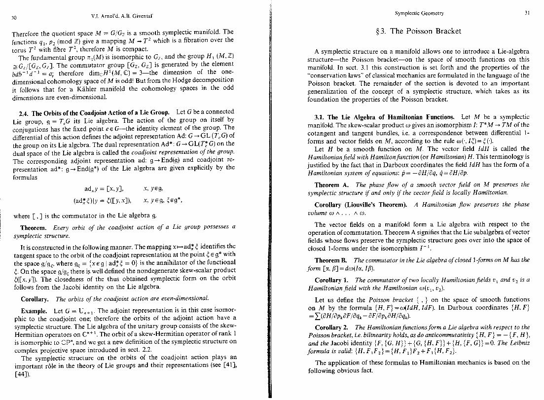
2.4. The Orbits of the Coadjoint Action of a Lie Group. Let G be a connected Lie group, g = T,G its Lie algebra. The action of the group on itself by conjugations has the fixed point e E G-the identity element of the group. The differential of this action defines the adjoint representation Ad: G + GL (T,G) of the group on its Lie algebra. The dual representation Ad*: G + GL(T: G) on the dual space of the Lie algebra is called the coadjoint representation of the group. The corresponding adjoint representation ad: g+ End(g) and coadjoint re- presentation ad*: g +End(g*) of the Lie algebra are given explicitly by the formulas
a&y = Cx, ~1, x, YE%32
WZ5)Iy = 5(Cy,xlh x, Y EC32 re3*,
where [ ,] is the commutator in the Lie algebra g.
Theorem. Every orbit of the coadjoint action of a Lie group possesses a symplectic structure.
It is constructed in the following manner. The mapping x++ad: 5 identifies the tangent space to the orbit of the coadjoint representation at the point 5 E g* with the space g/g+ where ge = {XE g 1 ad:< = 0} is the annihilator of the functional 5. On the space g/g< there is well defined the nondegenerate skew-scalar product <([x, y]). The closedness of the thus obtained symplectic form on the orbit follows from the Jacobi identity on the Lie algebra.
Corollary. The orbits of the coadjoint action are even-dimensional.
Example. Let G = U,, 1. The adjoint representation is in this case isomor- phic to the coadjoint one; therefore the orbits of the adjoint action have a symplectic structure. The Lie algebra of the unitary group consists of the skew- Hermitian operators on @” + ‘. The orbit of a skew-Hermitian operator of rank 1 is isomorphic to CP”, and we get a new definition of the symplectic structure on complex projective space introduced in sect. 2.2.
The symplectic structure on the orbits of the coadjoint action plays an important r61e in the theory of Lie groups and their representations (see [41], CW).
Symplectic Geometry 31
$3. The Poisson Bracket
A symplectic structure on a manifold allows one to introduce a Lie-algebra structure-the Poisson bracket-on the space of smooth functions on this manifold. In sect. 3.1 this construction is set forth and the properties of the “conservation laws” of classical mechanics are formulated in the language of the Poisson bracket. The remainder of the section is devoted to an important generalization of the concept of a symplectic structure, which takes as its foundation the properties of the Poisson bracket.
3.1. The Lie Algebra of Hamiltonian Functions. Let M be a symplectic manifold. The skew-scalar product o gives an isomorphism I: T*M + TM of the cotangent and tangent bundles, i.e. a correspondence between differential l- forms and vector fields on M, according to the rule o(., Z<) = < (.).
Let H be a smooth function on M. The vector field ZdH is called the Hamiltonianjield with Hamilton function (or Hamiltonian) H. This terminology is justified by the fact that in Darboux coordinates the field IdH has the form of a Hamiltonian system of equations: Ij = - aH/aq, 4 = aHlap.
Theorem A. The phase frow of a smooth vector field on M preserves the symplectic structure if and only if the vector field is locally Hamiltonian.
Corollary (Liouville’s Theorem). A Hamiltonian flow preserves the phase volume 0 A . . . A 0.
The vector fields on a manifold form a Lie algebra with respect to the operation of commutation. Theorem A signifies that the Lie subalgebra of vector fields whose Rows preserve the symplectic structure goes over into the space of closed l-forms under the isomorphism I-‘.
Theorem B. The commutator in the Lie algebra of closed l-forms on M has the form [cr, /3] =dw(lcc, I/3).
Corollary 1. The commutator of two locally Hamiltonianjields v1 and v2 is a Hamiltonianfield with the Hamiltonian w(v,, v2).
Let us define the Poisson bracket { , > on the space of smooth functions on M by the formula {H, F} =o(ZdH, IdF). In Darboux coordinates {H, F} =C(aHlap,aFlaq,-aaFlap,aHlaq,).
Corollary 2. The Hamiltonian functions form a Lie algebra with respect to the Poisson bracket, i.e. bilinearity holds, as do anticommutativity {H, F) = - (F, H >, and the Jacobi identity {F, (G, H)) + {G, {H, F}} + {H, (F, G}> =O. The Leibniz formula is valid: {H, FIF2} =(H, F,)F, + F,{H, F,).
The application of these formulas to Hamiltonian mechanics is based on the following obvious fact.

32 V.I. Amol’d, A.B. Givental’
Theorem C. The derivative of a function F along a vector field with a Hamiltonian H is equal to the Poisson bracket {H, F}.
Corollaries. a) The law of conservation of energy: a Hamiltonianfunction is a first integral of its HamiltonianJow.
b) The theorem of E. Noether: A Hamiltonian F whose flow preserves the Hamiltonian H is a first integral of the flow with Hamiltonian H.
c) The Poisson theorem: The Poisson bracket of two first integrals of a Hamiltonian flow is again a first integral.
Example. If in a mechanical system two components M,, M, of the angular momentum vector are conserved, then also the third one M3 = {M,, M2) will be conserved.
3.2. Poisson Manifolds. A Poisson structure on a manifold is a bilinear form ( , } on the space of smooth functions on it satisfying the requirement of anticommutativity, the Jacobi identity and the Leibniz rule (see corollary 2 of the preceding item). This form we shall still call a Poisson bracket. The first two properties of the Poisson bracket mean that it gives a Lie algebra structure on the space of smooth functions on the manifold. From the Leibniz rule it follows that the Poisson bracket of an arbitrary function with a function having a second- order zero at a given point vanishes at this point; therefore a Poisson structure defines an exterior 2-form on each cotangent space to the manifold, depending smoothly on the point of application. Conversely, the value of such a 2-form on a pair df, dg of differentials of functions defines a skew-symmetric biderivation (A g)++ W(f, g) of the functions, that is, a bilinear skew-symmetric operation satisfying the Leibniz identity with respect to each argument.
On a manifold let there be given two smooth fields V and W of exterior 2- forms on the cotangent bundle. We designate as their Schouten bracket [V, W] the smooth field of trilinear forms on the cotangent bundle defined by the following formula
EJ’, W(f,s,h)=Vf, V’Y(g,hN+WS, W,W+ . . . > where the dots denote the terms with cyclically permutedf, g and h.
Lemma. A smooth jield W of exterior 2-forms on the cotangent spaces to a manifold gives a Poisson structure on it if and only if [W, W] =O.
In coordinates a Poisson structure is given by a tensor xwij(a/8xi) A (a/ax,), where the wij are smooth functions satisfying the conditions: for all i, j, k wij= - Wji and
A Poisson structure, like a symplectic one, defines a homomorphism of the Lie algebra of smooth functions into the Lie algebra of vector fields on the manifold:
Symplectic Geometry 33
the derivative of a function g along the field of the function f is equal to {J g}. Such fields are called Hamiltonian; their flows preserve the Poisson structure. Hamiltonians to which zero fields correspond are called Casimirfunctions and they form the centre of the Lie algebra of functions. In contrast to the nondegenerate symplectic case, the centre need not consist only of locally constant functions.
The following theorem aids in understanding the structure of Poisson manifolds and their connection with symplectic ones. Let us call two points of a Poisson manifold equivalent if there exists a piecewise smooth curve joining them, each segment of which is a trajectory of a Hamiltonian vector field. The vectors of Hamiltonian fields generate a tangent subspace at each point of the Poisson manifold. Its dimension is called the rank of the Poisson structure at the given point and is equal to the rank of the skew-symmetric 2-form defined on the cotangent space.
The Foliation Theorem ([42], [74]). The equivalence class of an arbitrary point of a Poisson manifold is a symplectic submanifold of a dimension equal to the rank of the Poisson structure at that point.
Thus, a Poisson manifold breaks up into symplectic leaves, which in aggregate determine the Poisson structure: the Poisson bracket of two functions can be computed over their restrictions to the symplectic leaves. A transversal to a symplectic leaf at any point intersects the neighbouring symplectic leaves transversally along symplectic manifolds and inherits a Poisson structure in a neighbourhood of the original point.
The Splitting Theorem ([74]). The germ ofa Poisson manifold at any point is isomorphic (as a Poisson manifold) to the product of the germ ofthe symplectic leaf with the germ of the transversal Poisson manifold of this point. The latter is uniquely determined up to isomorphism of germs of Poisson manifolds.
This theorem reduces the study of Poisson manifolds in the neighbourhood of a point to the case of a point of rank zero.
3.3. Linear Poisson Structures. A Poisson structure on a vector space is called linear if the Poisson bracket of linear functions is again linear. A linear Poisson structure on a vector space is precisely a Lie algebra structure on the dual space; the symplectic leaves of the linear structure are the orbits of the coadjoint action of this Lie algebra, the Casimir functions are the invariants of this action.
At a point x of rank 0 on a Poisson manifold there is well defined the linear approximation of the Poisson structure-a linear Poisson structure on the tangent space of this point (or a Lie algebra structure on the cotangent space): C&L dxgl =d.xLh s>-

34 V.I. Amol’d, A.B. Givental’
The Annihilator Theorem. Let g be a Lie algebra, let 5 E g*, and let gs =
{x E glad:< =0} be the annihilator of g in g. The linear approximation of the
transversal Poisson structure to the orbit of the coadjoint action at the point < is canonically isomorphic to the linear Poisson structure on the dual space of the annihilator SC.
The isomorphism is given by the mapping g*/ad,*< -gF of the spaces of definition of the linear Poisson structures being regarded which is dual to the inclusion g: 4 g.
Corollary 1. Each element of a semisimple Lie algebra of rank r is contained in an r-dimensional commutatiz;e subalgebra.
Proof: 1”. One of the possible definitions of a semisimple Lie algebra consists in the nondegeneracy of its Killing form (x, y) = tr(ad,O ad,,). This form is invariant with respect to the adjoint action; therefore the adjoint representation of a semisimple Lie algebra is isomorphic to the coadjoint one.
2”. By the rank of a Lie algebra is meant the codimension of a generic orbit of the coadjoint action (i.e. the corank of its Poisson structure at a generic point). It follows from the annihilator theorem that the rank of the annihilator gg of an arbitrary <ES* is not less than the rank of g. Indeed, upon linearization the codimension of a generic symplectic leaf can only increase!
3”. Duflo’s Theorem. The annihilator of a generic element 5 E g* is commuta- tive. In fact, the symplectic leaves of the transversal Poisson structure at a generic point < are zero-dimensional, and the theorem follows from 2”. Let us note that the dimension of such an annihilator is equal to the rank of the Lie algebra g.
4”. Corollary 1 is obtained by an application of 3” to the annihilator gx of the element x E g with respect to the adjoint action, in view of the fact that x lies in the centre of the algebra gx. 0
Corollary 2. A linear Hamiltonian system on R’” has n linearly independent quadratic first integrals.
Indeed, sp(2n, R) is a simple Lie algebra of rank n. 0
3.4. The Linearization Problem. In connection with Poisson structures this problem can be stated thus: is a Poisson structure isomorphic in a neighbour- hood of a point of rank 0 to its linear approximation at that point? All the previous results of the section were equally true both in the smooth and in the holomorphic case, while the answer to this question may depend on the category in which the linearization is carried out.
We shall call a Lie algebra g (analytically, Cm-) sufficient if any Poisson structure whose linear approximation at a point of rank 0 is isomorphic to g* is itself (analytically, Cm-) isomorphic to g * in a neighbourhood of this point.
This definition is in keeping with the general approach to linearization problems in analysis: linearizability is treated as a property of the linear approximation.
Symplectic Geometry 35
The description of sufficient Lie algebras is an open problem. It is easy to convince oneself that commutative Lie algebras are not sufficient in either of the two indicated senses. The solvable two-dimensional Lie algebra of the group of affine transformations of the line is sufficient in each of them. The semisimple Lie algebra sl&R) of the group of symplectomorphisms of the plane is analytically sufficient, but is not (F-sufficient.
Theorem ([17]). A semisimple (real or complex) Lie algebra is analytically suficient. A semisimple Lie algebra of a compact group is C”-suJficient.
Let us observe that linearization of a germ of a Poisson structure with a semisimple linear approximation is equivalent to the selection, in the Lie algebra of Hamiltonian functions, of a semisimple complement to its radical--the nilpotent ideal consisting of the functions with a second-order zero at the coordinate origin. Therefore linearizability modulo terms of sufficiently high order follows from the theorem of Levi-Mal’tsev, which asserts the existence of such a complement in the case of finite-dimensional Lie algebras.
$4. Lagrangian Submanifolds and Fibrations
A submanifold of a symplectic manifold (MZ”, w) is called Lagrangian if it has dimension n and the restriction to it of the symplectic form o is equal to 0. Using the terminology of 9 1 of Chapter 1, one may say that Lagrangianity of a submanifold is just Lagrangianity of its tangent spaces. More generally, a submanifold of a symplectic manifold is called (co)isotropic6 if its tangent spaces are so.
4.1. Examples of Lagrangian Manifolds. 1) A smooth curve on a symplectic surface is Lagrangian. A smooth curve on a symplectic manifold is isotropic and a hypersurface is coisotropic.
2) Let M= T*X, let tl be the action l-form on M and o=dcc the canonical symplectic structure. A l-form on a manifold associates to a point of the manifold a covector at that point. We shall speak of the graph of the l-form to mean the totality of these covectors. The graph of a closed l-form on X is a Lagrangian submanifold of M. Indeed, the restriction of the symplectic form o=d(pdq) to the graph of the l-form t:q~p(q) is equal to d(p(q) dq)=dt=O if 5 is closed. Conversely, a Lagrangian submanifold in M which projects one-to-one onto the base is the graph of a closed l-form on X. If this l-form is exact, 5 = d4, then its potential 4 is called a generatingfunction of the Lagrangian submanifold. This example suggests definition of a generalized function on X as an arbitrary Lagrangian submanifold in T*X. A fibre of the cotangent bundle is also Lagrangian and corresponds to the “delta function” of the point of application.
6 Coisotropic submanifolds are also called involutive.
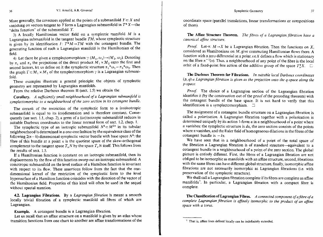
36 V.I. Amol’d, A.B. Givental
More generally, the covectors applied at the points of a submanifold Y c X and vanishing on vectors tangent to Y form a Lagrangian submanifold in T* X-the “delta function” of the submanifold Y.
3) A locally Hamiltonian vector field on a symplectic manifold M is a Lagrangian submanifold in the tangent bundle TM, whose symplectic structure is given by its identification I: T*M -+TM with the cotangent bundle. The generating function of such a Lagrangian manifold is the Hamiltonian of the field.
4) Let there be given a symplectomorphism y: (M,, o~)+(M~, 02). Denoting by rci and 7c2 the projections of the direct product M, x M, onto the first and second factors, let us define on it the symplectic structure 7c1*w1 -7cZ*02. Then the graph I’ c M1 x M2 of the symplectomorphism y is a Lagrangian submani- fold.
These examples illustrate a general principle: the objects of symplectic geometry are represented by Lagrangian manifolds.
From the relative Darboux theorem II (sect. 1.5) we obtain the
Corollary. A suficiently small neighbourhood of a Lagrangian submangold is symplectomorphic to a neighbourhood of the zero section in its cotangent bundle.
The corank of the restriction of the symplectic form to a (co)isotropic submanifold is equal to its (co)dimension and is therefore constant. Conse- quently (see sect. 1.1, chap. 2), a germ of a (co)isotropic submanifold reduces in suitable Darboux coordinates to the linear normal form of sect. 1.2, chap. 1.
The symplectic type of an isotropic submanifold Nkc M2” in its tubular neighbourhood is determined in a one-one fashion by the equivalence class of the following 2(n - k)-dimensional symplectic vector bundle with base space Nk: the fibre of this bundle at a point x is the quotient space of the skew-orthogonal complement to the tangent space T, N by the space T, N itself. This follows from the results of sect. 1.5.
If a Hamiltonian function is constant on an isotropic submanifold, then its displacements by the flow of this function sweep out an isotropic submanifold. A coisotropic submanifold on the level surface of a Hamilton function is invariant with respect to its flow. These assertions follow from the fact that the one- dimensional kernel of the restriction of the symplectic form to the level hypersurface of a Hamilton function coincides with the direction of the vector of the Hamiltonian field. Properties of this kind will often be used in the sequel without special mention.
4.2. Lagrangian Fibrations. By a Lagrangian jibration is meant a smooth locally trivial fibration of a symplectic manifold all fibres of which are Lagrangian.
Example. A cotangent bundle is a Lagrangian fibration. Let us recall that an affine structure on a manifold is given by an atlas whose
transition functions from one chart to another are affine transformations of the
Symplectic Geometry 37
coordinate space (parallel translations, linear transformations or compositions of them).
The Afine Structure Theorem. The jibres of a Lagrangian jbration have a canonical a&fine structure,
Proof Let-r: M-+X be a Lagrangian fibration. Then the functions on X, considered as Hamiltonians on M, give commuting Hamiltonian flows there. A function with a zero differential at a point XEX defines a flow which is stationary on the fibre rt- l(x). Thus, a neighbourhood of any point of the fibre is the local orbit of a fixed-point free action of the additive group of the space T,*X. C
The Darboux Theorem for Fibrations. In suitable local Darboux coordinates (p, q) a LagrangianJibration is given as the projection onto the q-space along the p-space.
Proof: The choice of a Lagrangian section of the Lagrangian fibration identifies it (by the construction out of the proof of the preceding theorem) with the cotangent bundle of the base space. It is not hard to verify that this identification is a symplectomorphism. 0
The assignment of a cotangent bundle structure on a Lagrangian fibration is called a polarization. A Lagrangian fibration together with a polarization is determined uniquely by its action l-form a in a neighbourhood of a point where c( vanishes: the symplectic structure is dcr, the zero section consists of the points where CI vanishes, and the Euler field of homogeneous dilations in the fibres of the cotangent bundle is -la.
We have seen that in a neighbourhood of a point of the total space of the fibration a Lagrangian fibration is of standard structure-equivalent to a cotangent bundle in a neighbourhood of a point of the zero section. The global picture is entirely different. First, the fibres of a Lagrangian fibration are not obliged to be isomorphic as manifolds with an affine structure, second, fibrations with the same fibres can have different global structure, finally, isomorphic affine fibrations are not necessarily isomorphic as Lagrangian fibrations (i.e. with preservation of the symplectic structure).
We shall call a Lagrangian fibration complete if its fibres are complete as affine manifolds’. In particular, a Lagrangian fibration with a compact fibre is complete.
The Classification of Lagrangian Fibres. A connected component of afibre of a complete Lagrangianfibration is afinely isomorphic to the product of an afJine space with a torus.
’ That is, affine lines defined locally can be indefinitely extended.

38 V.I. Arnol’d, A.B. Givental’
Indeed, the completeness of the fibration means that every component of the fibre is a quotient space of the group of translations R” by a discrete subgroup. The only such subgroups are the lattices Zk c 1w”, k 5 n.
Corollary. A connected compact fibre of a Lagrangian jibration is a torus.
Let us now describe the complete Lagrangian fibrations with an affine fibre. A twisted cotangent bundle is a cotangent bundle rr: T*X+X with a symplectic structure on T*X equal to the sum of the canonical symplectic form and a form rr*$, where 4 is a closed 2-form on the base space X. We have already encountered this construction at the end of 5 1.
Theorem. A twisted cotangent bundle is determined by the cohomology class of the form q5 in H2(X, 52) uniquely up to an isomorphism of Lagrangian fibrations (which is the identity on the base space). Any complete Lagrangianjbration with a connected, simply connected jibre is isomorphic to a twisted cotangent bundle.
Proof: Let rr: (M, u)+X be a Lagrangian fibration whose fibres are affine spaces. A section s: X 4 M defines a closed form 4 = s*w and o -rr*$ is a symplectic structure on M in which s(X) is Lagrangian. Taking s as the zero section, by the construction of the affine structure theorem we identify M with T*X. A change of the zero section by s’ changes 4 by ds’; therefore the class [c$]EH~(X, R) is the only invariant of the twisted cotangent bundle. 0
We have already come across an example of a topologically nontrivial Lagrangian fibration with a compact fibre in sect. 2.3 on Klhler structures: we presented a symplectic manifold M4, a Lagrangian fibration over the torus T2 with fibre T2, not homeomorphic to T2 x T2. It turns out the compactness of the fibre of a Lagrangian fibration imposes very stringent conditions on its base space.
Theorem. The base space of a Lagrangianjibration with a connected compact fibre has a canonical integral a&e structure (in other words, in some atlas on the base space the transition functions are compositions of translations and integral linear transformations on KY).
Proof: The identification of the fibre T” over a point x of the base space X with an orbit of the group T,*X gives on T:X a lattice of maximal rank. A continuous basis of such a lattice is a set of l-forms c~i, . . . , a, on X. The symplecticity of translations by the lattice vectors in T*X means that these forms are closed. The local potential (41, . . . , 4”): X + R” of this basis, d4i = ai, defines a chart of the desired atlas. 0
4.3. Intersections of Lagrangian Manifolds and Fixed Points of Symplecto- morphisms. The problem of the existence of periodic motions of dynamical systems led H. Poincare to the following theorem.
Symplectic Geometry 39
Poincarb’s Geometric Theorem. A homeomorphism of a plane circular annulus onto itself which preserves areas and which moves the boundary circles in d@erent directions has at least two fixed points.
The boundary condition in the theorem means that the mapping has the form X=x +f(x, y), Y=y +g(x, y), where X, x are radial coordinates and Y, y are angular coordinates on the annulus, and the functionsf, g are continuous and 27r- periodic in y, and moreover g has different signs on the different boundaries of the annulus.
The proof of this theorem is due to G.D. Birkhoff. H. Poincare succeeded in proving it only under certain restrictions, but his method is less special than Birkhoff’s proof and lends itself to generalization. Poincart’s argument is based on the fact that the fixed points of a symplectomorphism of the annulus are precisely the critical points of the function F(u, u)=f(Jdu-gdu), where u=(X +x)/2, u=( Y+ y)/2, true under the assumption that the Jacobian a(u, u)/c?(x, y) is different from zero. This condition is automatically fulfilled if the symplectomorphism is not too far from the identity.
Carrying over PoincaSs arguments to the general symplectic situation leads to the following concepts and results.
Let M be a symplectic manifold. A symplectomorphism y: M+M is given by a Lagrangian graph Tc M x M. A fixed point of ‘/ is an intersection point of I- with the graph A of the identity symplectomorphism. A tubular neighbourhood of A in M x M has the structure of the Lagrangian bundle T*A. If the symplectomorphism 7 is sufficiently close to the identity, then it is given by a generating function (generally speaking, by a many-valued one) of the Lagrangian section r c T*A. Its critical points and the fixed points of y coincide.
We shall say that a symplectomorphism y is homologous to the identity if it can be connected with the identity by a family of symplectomorphisms whose velocity field for each value of the parameter of the family is globally Hamiltonian. The symplectomorphisms homologous to the identity form the commutator subgroup of the identity component of the group of symplecto- morphisms of the manifold M.
Lemma. A symplectomorphism which is homologous to and close (together with i&first derivatives) to the identity has a single-valued generating function.
Theorem A, A symplectomorphism of a compact symplectic manifold which is homologous to and close to the identity has fixed points. Their number is not less than the number of critical points which a smooth function on this manifold must have at the very least.
Conjecture A. The preceding theorem is true without the condition of closeness of the symplectomorphism to the identity.
The conjecture has been proved in the two-dimensional case: a symplecto- morphism of a compact surface homologous to the identity has for the sphere not less than 2, and in the case of the sphere with handles not less than 3 fixed

40 V.I. Arnol’d, A.B. Givental’
points. The proof of these theorems * bears an essentially two-dimensional character. Thus, in the case of the sphere the proof is based on the fact that the index of an isolated singular point of a Hamiltonian vector field on the plane is equal to one minus one-half the number of components into which the critical level curve of the Hamiltonian divides a neighbourhood of the singular point and hence does not exceed 1.
Let us observe that Poincarl’s theorem on the symplectomorphism of the annulus follows from the (proven) conjecture A for the two-dimensional torus. Out of two copies of the annulus one can glue together a torus. The sym- plectomorphisms of the torus lR2/Z2 homologous to the identity are precisely those which leave in place the centre of gravity of the unit square in [w2 [2]. The latter is not difficult to achieve if one adds connective strips between the glued- together annuli and extends the symplectomorphism so as not to have fixed points on these strips (here it will be necessary to use the rotation of the boundaries of the annulus in different directions).
We shall call two Lagrangian submanifolds of a symplectic manifold N (Lagrangianly) isotopic if one goes over into the other under the action of a symplectomorphism homologous to the identity. In particular, isotopic Lagrangian submanifolds are diffeomorphic.
Theorem B. A compact Lagrangian submanifold isotopic to and close to a given one has as many points of intersection with it as some smooth function on this manifold has critical points.
Conjecture B. Theorem B is true without the assumption of closeness of the isotopic Lagrangian submanifolds.
Conjecture (theorem) A follows out of conjecture (theorem) B: the graph r c M x M of a symplectomorphism y: M +M homologous to the identity is a Lagrangian submanifold isotopic to the diagonal A.
Without the isotopy assumption intersection points of a compact Lagrangian submanifold with a Lagrangian perturbation of it (of which it is the question in theorem B) may be absent. Nevertheless intersection points necessarily exist if the Euler characteristic of the Lagrangian manifold is different from 0 or if each closed l-form on this manifold is the differential of a function. It turns out that the absence of intersection points of a compact Lagrangian submanifold with its Lagrangian perturbation means that this manifold is fibred over a circle.
By a new method progress was recently achieved in the proof of conjectures A and B in the many-dimensional case. Namely, conjecture A has been proved for symplectomorphisms of the torus T2”= R2”/Z2” with the standard symplectic structure, just as conjecture B has been proved for the Lagrangian torus T” embedded in the standard symplectic torus T2” as a subgroup and for an arbitrary Lagrangian isotopy of the torus T” [19]. Let us note that a smooth
s The first is due to A.I. Shnirel’man and N.A. Nikishin, the second to Ya.M. Ehliashberg.
Symplectic Geometry 41
function on the n-dimensional torus has no fewer than n + 1 critical points and no fewer than 2”, counting them with multiplicities [24].
To demonstrate the essence of the method, we shall give a sketch of the proof of the following assertion.
Theorem. On the standard symplectic Zn-dimensional torus let there be given a Hamiltonian depending periodically on time. Then the symplectic transformation of the torus after a period by thejlow of this Hamiltonian has at least onejxed point.
lo. Representing T2” as the quotient space [w2”/Z2” of the standard symplectic space 5X2”, let us consider the vector space Q of loops-smooth mappings of lR/Z+[W2”-with the linear structure of pointwise addition and scalar multiplica-
tion and with the Euclidean structure j (p2 + q2)/2dt. On the space Q let us
introduce the action functional F= s [(pdq -qdp)/2- Hdt], where H(p, q, t) is
the given periodic Hamiltonian with period 1. To the various critical points of the functional F: R+ 1w correspond the various periodic trajectories with period 1 of the flow of the Hamiltonian H, i.e. the various fixed points of the sym- plectomorphism we are interested in.
2”. The gradient VF: Q+R has the form VF = - Jdldt-VH, where J:
IW2”-+ iw”’ is the operator “multiplication by J-1”, J(p, q) = (- q, p). We regard the mapping VF as a perturbation of the linear operator A= - Jdldt. The spectrum of the operator A is 2nZ, and the eigenspace with the eigenvalue ;i is the 2n-dimensional space of solutions with period 1 of the linear Hamiltonian system with Hamiltonian L(p2 + q2)/2. The expansion of a loop [w/Z-+[w2” by eigenfunctions of the operator A is simply its Fourier series expansion. The perturbation B=VH has a bounded image (11 B(o)11 <C) and a bounded norm: II&q)-W,)II s ~llQ4 -wzII.
3”. Let us represent the space Q in the form of a direct sum of a finite- dimensional space V, spanned by the “lower harmonics” with frequency I %I < 20, and an infinite-dimensional space W of “higher harmonics”. The equation VF=O splits into two: aF/aV=O and aF/aW=O. The second has the form Aw + P B(v + w) =O, where P is the projector of R onto W. Since the operator WI+ -A- ‘PB(v+ w) is contracting, the second equation has for each v a unique solution w = w(u). Therefore the search for extrema of the functional F reduces to the determination of the critical points of the function f(u)= F(v, w(u)) on the finite-dimensional space.
4”. The constant loops, which form the kernel of the operator A, correspond to the zero solution of the equation aF/a W= 0; therefore the functionf is periodic on the subspace of such loops. Thus the functionf, essentially, is defined on the manifold T2” x RN /.>o x w<o. Its behaviour at infinity is determined by the unperturbed functional and has hyperbolic character (Fig. 1 l), from which the presence of critical points follows (for example, the set of points where the value

42 V.I. Amol’d, A.B. Givental’
Fig. 11. The change of structure of the level topology of the function f
of the function is less than a given value undergoes a topological change of structure).
Remark. Further analysis of this finite-dimensional situation with tools developed in Morse theory ([SS]) leads to an exact estimate of the number of fixed points (2 2n + 1). The fundamental difference of the argument cited to the standard formalism of the global variational calculus consists in the fact that the unperturbed quadratic functional on the loop space is not elliptic but hyperbolic.
Chapter 3
Symplectic Geometry and Mechanics
Here we shall examine the connection of symplectic geometry with the variational calculus, in particular, with Lagrangian mechanics, we shall give a geometric introduction to the theory of completely integrable systems, and we shall describe a procedure for reducing the order of Hamiltonian systems having a continuous symmetry group. For a systematic exposition of the questions of classical mechanics see volume 3, and for the theory of integrable systems see the article by B.A. Dubrovin, I.M. Krichever and S.P. Novikov in this volume.
0 1. Variational Principles
The motions of a mechanical system are the extremals of a suitable variational principle. On the other hand, any problem of the calculus of variations can be formulated in the language of symplectic geometry.
Symplectic Geometry 43
1.1. Lagrangian Mechanics. A natural mechanical system is given by a kinetic and a potential energy. The potential energy is a smooth function on the manifold ofconjgurations (states) of the system, the kinetic energy is a Riemannian metric on the configuration manifold, i.e. a positive definite quadratic form on each tangent space to the manifold ofconfigurations depending smoothly on the point of application.
Example. A system of mass points in Euclidean space has the kinetic energy T=xm,i,2/2 and the potential energy U =I V,, (rk-rI), where rk is the radius vector of the kth point and V,, is the potential of the pairwise interaction of the mass points, say the Newtonian gravitational potential Vkl(r)= -;jm,m,//rl.
Out of the kinetic and potential energies one composes the Lagrangian or Lagrange function L= T-U on the total space of the tangent bundle of the configuration manifold. A motion t-q(t) of a natural system in the configur- ation space is an extremal of the functional
More generally, if we consider an arbitrary Lagrange function L: TM+[w on the tangent bundle of the configuration manifold and if we designate as motions the extremals of the functional (I), we obtain the definition of a Lagranyian mechanical system. One may also assume an explicit dependence of the Lagrangian on time. The extremals of the functional (1) are locally described by the system of Euler-Lagrange differential equations (d/dt)aL/&j = dL/aq. For a system of mass points in Euclidean space the Euler-Lagrange equations take the form of the system of Newton’s equations m,F,= -dU/&,. Thus, Lagrangian mechanics generalizes Newtonian mechanics, admitting into consideration, for example, systems of mass points with holonomic (rigid) constraints- the configuration manifolds of such systems are no longer domains of coordinate spaces. At the same time, the Lagrangian approach to mechanics permits considering it as a special case of the variational calculus. For example, the problem of the “free” motion of a natural system (U - 0) is equivalent to the description of the geodesic flow on a configuration manifold with Riemannian metric T (see sect. 1.3).
Example. Let us consider an absolutely rigid body one of whose points is fastened at the coordinate origin of the space iw3. The configuration manifold of such a system is the rotation group SO,. The tangent space to the configuration manifold at each point can be identified with the space Iw3: the direction of the vector OG[W~ indicates the axis and the direction of the infinitesimal rotation of the body, and the length of the vector indicates the angular velocity of the rotation. The kinetic energy of the rotation is T= lw2/2, where I is the moment of inertia of the body with respect to the axis of rotation, i.e. the kinetic energy is given in the internal coordinates of the body by the inertia quadratic form. Thus the free rotation of a rigid body fixed at a point is described by the geodesic flow

44 V.I. Amol’d, A.B. Givental’
on the group SO, of a Riemannian metric (left-)invariant with respect to the translations on the group.
1.2. Hamiltonian Mechanics. A Hamiltonian mechanical system is given by a smooth function-the Hamiltonian-on a symplectic manifold (the phase space). The motion in the Hamiltonian system is described by the phase flow of the corresponding Hamiltonian vector field (see sect. 3.1, chap. 2). A Hamilton- ian H depending explicitly on time gives a nonautonomous Hamiltonian system. In Darboux coordinates the system of Hamilton’s equations has the form p= -H,,q=H
Hamiltonian kechanics generalizes Lagrangian mechanics.
Example 1. The system of Euler-Lagrange equations of a natural system with configuration manifold M, kinetic energy T and potential energy U is converted, under the isomorphism of the tangent and cotangent bundles of the manifold M defined by the Riemannian metric 2T, into a system of Hamilton’s equations with Hamiltonian T+ U with respect to the canonical symplectic structure on the total space of the cotangent bundle.
In the general case let us define the Hamiltonian H: T*M-+R as the fibrewise Legendre transformation of the Lagrangian L: TM + R. The Legendre transformation of a convex function f of the vector argument t’ is defined as a function f* of the dual argument p by the formula f*(p)=max [(p, v) -.f(v)]
(Fig. 12, compare sect. 1.1, chap. 5). For example, the Legendre’iransformation of the Euclidean form (Au, v )/2 is (p, A - ’ p )/2.
We shall suppose that the mapping T,M-, T$ M: QHP= L4 is a diffeo- morphism for each q~ M. Then the Hamiltonian H is a smooth function on the total space of the cotangent bundle, H(p, q) = pq - L(q, 4), where 4 is determined from the equation p= L,(q, 4).
Theorem. Under the indicated identification of the total spaces of the tangent and cotangent bundles the mechanical system with Lugrungiunfunction L goes over into the Hamiltonian system with Hamiltonian H.
Fig. 12. The Legendre transformation
Symplectic Geometry 45
Example 2. A natural system in a magnetic field. Let the Lagrangian be the sum of the Lagrangian of a natural system and a differential l-form A on the configuration manifold M, regarded as a function on TM linear with respect to the velocities: L = T- U + A. The corresponding system of Euler-Lagrange equations on TM is Hamiltonian with Hamiltonian function H = T+ U with respect to the symplectic structure R + dA, where Q is the symplectic structure of example 1. If the 1 -form A is a many-valued “vector-potential of a magnetic field” dA defined single-valuedly on M, then the phase space turns out to be a twisted cotangent bundle (sect. 4.2, chap. 2).
1.3. The Principle of Least Action. The fact that the problems of the calculus of variations have a Hamiltonian character is explained by the presence of a variational principle in the Hamiltonian formalism itself. At the basis of this principle lies the following observation: the field of directions of a Hamiltonian vector field on a nonsingular level hypersurface of its Hamiltonian coincides with the jield of characteristic directions of this hypersurfuce- the field of skew- orthogonal complements of its tangent hyperplanes.
Let the symplectic manifold M be polarized: M = T*B, and let c1= 1 p,dq, be the action l-form on M.
Theorem (The principle of least action). The integral curves of the field of characteristic directions of a nonsingular hypersurfuce IY c T*B transversal to the fibres of the cotangent bundle T*B+B are extremuls of the action integral sa in the class of curves lying on I- and joining thefibres T4*, B and Tz, B of the points q,, and q1 of the base space B.
Proof: The increment of the action integral [ a--J a (Fig. 13) is equal to the
symplectic area of the sheet joining two curves “J &d y’:‘and in the case that y is an
r
%I iJ e, Fig. 13. The proof of the principle of least action

46 V.I. Arnol’d, A.B. Givental‘
integral curve, it is infinitesimal to a higher order than the difference of the curves y and 7’. G
Remark. The integral curves of a nonautonomous system of equations with the Hamiltonian function H(p, 4, t) in the extended phase space iw” * x iw” x Iw are
extremals of the action integral i (pdq - Hdr) in the class of curves t H( p(t), q(r), t)
with the boundary conditions z(r,) = qO, q(tl ) = ql.
Corollary. A mass pointforced to stay on a smooth Riemann manifold moves on geodesic curves (i.e. on extremals gf the length Ids).
In fact, in the case of free motion with kinetic energy T=(ds/dr)‘/2 the parameter t ensuring a fixed value of the energy H = T= h must be proportional to the length, dt =ds/fi, and the action integral takes the form f pdq=S pQdt
=JZTdt=,/%j-ds. In the case where the potential energy is different from zero, the trajectories of
a natural system are also geodesics of a certain Riemannian metric: in the region of the configuration space where U(q) < h the trajectories of a system with kinetic energy T=(ds/dt)2/2, potential energy U(q) and total energy h will be geodesic curves of the metric (h- U(q))ds’.
As an application let us consider the rotation of a rigid body around a fixed point in a potential field. For sufficiently large h the Rjemannian metric (h - U)ds2 is defined on the whole compact configuration space SO,. The space SO, is not simply connected (it is diffeomorphic to Rp3 and has a simply connected double covering by S3).
In the class of all noncontractible closed curves on SO, let us choose a curve of minimal length (this is possible [SS]) with respect to the Riemann metric introduced above. We obtain the
Corollary. A rigid body in an arbitrary potential,field has at least one periodic motion for each sujficiently large value qf the total energy.
One can show [55] that on a compact Riemannian manifold each element of the fundamental group is represented by a closed geodesic. From this one can obtain an analog of the preceding corollary for an arbitrary natural system with a compact non-simply connected configuration space.
1.4. Variational Problems with Higher Derivatives. Let us describe the Hamiltonian formalism of the problem of minimizing the functional
i L(x’O’, . _ . , x(“+ “)dt (2)
within the class of smooth curves x: iw +iw’ with a given Taylor expansion at the ends of the interval [a, h] up to order n inclusive, where the Lagrangian L depends on the derivatives x (k)=dkx/dtk of the curve x(t) up to order n+ 1. The
Symplectic Geometry
extremals of the functional (2) satisfy the system of Euler-Poisson equations
d”+1
L.~,,l-~L~,,~+~L,:,- . . .+(-l)“+‘~LX,..,,=o,
47
which expresses the vanishing of the first variation of the functional (2). Now let us regard the Lagrangian L(x, y, , Z, w) as a function of a point on a curve (x, y, . ) z, w): R-+R(“+2)f satisfying the restrictions dx = ydt, . . . , dz = wdt, and let us put together the action form according to the Lagrange multiplier rule:
r=p,(dx-ydt)+ . +p,(dz-wdt)+Ldt
=[p,(i-y)+ . . . +p,(i-w)+L(x,y,. . . , z, w)]dt.
The extremals of the functional JX satisfy the system of Euler-Lagrange equations in iW(2n+ 3)1:
i=y,. . . ) dL j=w; jxZFr OX
dL pp=-px+--,. . . ,p== .,o=-,=+g.
dY
This system is equivalent to the system of Euler-Poisson equations (3). Let us introduce the symplectic form w=dp, A dx+ . . +dp, A dz and with the aid of a Legendre transformation with respect to the variable w let us define the Hamiltonian function H (x, y, . . . , z, p=, . . . , py, p,)=p,y + . . . +p, W -L(x, Y, . . ., 5 W) (W(% Y, . > z, p,) is determined from the equation p==dL/8w). The system of Hamilton’s equations with the Hamiltonian H and the symplectic structure o on iw W+‘V together with the equation pZ=aL/aw coincides with (4). Thus, under the condition of convexity of the Lagrangian L(x’O’, . . . ) XC”+ 1’) with respect to the variable x(“+l), the system of Euler-Poisson equations (3) is equivalent to the Hamiltonian system (H, w).
Having thus written out the coordinate formulas, we shall now impart an invariant sense both to the variational problem (2) itself as well as to its Hamiltonian version.
Upon replacement of the space Iw’ by an arbitrary I-dimensional manifold M it is natural to give the functional of type (2) by means of a Lagrange function L: J”+ ’ -+ (w on the manifold of n + 1 -jets at 0 of curves x: IW-+M. The manifold J “+I is defined by induction together with the projection Jnfl +J” (Fig. 14) as the affine subbundle of the tangent bundle TJ” consisting of those ‘tangent vectors SET~,J” whi~ch under the differential x*: Tjn J” + T,, j”lJn-l of the projection 7~: J”+J”-’ go over into their point of application: ~c*(~)=~“ETJ”- ‘. In addition Jo = M, J ’ = TM.
The phase space of the Hamiltonian system corresponding to the Lagrangian L: J”+ ’ +[w is the total space T*J” of the cotangent bundle with the canonical symplectic structure. Let the function L be convex on each affine fibre of the fibre

48 V.I. Arnol’d, A.B. Givental
Jn+l -Jn T Jn-j - --- -J' --r) JO=M
Fig. 14. The definition of the jet spaces of curves
bundle J n+ ’ -+ J”. Let us construct a function H: T*J”+ R as follows. A covector p applied at the point ~GJ” defines a Iinear nonhomogeneous function on the fibre WC TjJ” of the bundle Jn+’ -+ J”. Let us set H(p) = max(p(w) - L(w)).
WEW
Ostrogradskij’s Theorem. The system of Euler-Poisson equations which is satisfied by the extremals of the Lagrangian L: J”+’ +Iw, where L is a smooth function, strictly convex’ on eachJibre of thefibre bundle J”+ ’ -+ J”, is equivalent to the Hamiltonian system with phase space T*J” and Hamiltonian function H.
Remark. In the case of explicit dependence of the Lagrangian in the functional (2) on time the system of Euler-Poisson equations is equivalent to the nonautonomous Hamiltonian system on the extended phase space Iw x T*J”.
1.5. The Manifold of Characteristics. Let us suppose that the integral curves of the field of characteristic directions on a smooth hypersurface in a symplectic manifold form a smooth manifold (locally this is always so). We shall call it the manifold of characteristics.
Theorem. The man$old of characteristics has a symplectic structure (it is well defined by the condition; the skew-scalar product of vectors tangent to the hypersurface is equal to the skew-scalar product of their projections along the characteristics).
Let the Hamiltonian system with Hamiltonian H have a first integral F, and let M be the manifold of characteristics of a hypersurface F = const. The function H is constant on the characteristics of this hypersurface and defines a smooth function I? on M. The field of the Hamiltonian H on the hypersurface F = const defines, upon projection onto M, a Hamiltonian vector field on M with Hamiltonian Ei.
Corollary 1. A first integral of a Hamiltonian system allows one to reduce its order by 2.
’ That is, d’(L(,)>O.
Symplectic Geometry 49
The parametrized extremals of a variational problem (possibly a non- autonomous one) form a symplectic manifold, namely the phase space of the corresponding Hamiltonian system (for example, T*J” for problem (2)). From the theorem we get
Corollary 2. If the oriented geodesics (the unparametrized ones) of a Riemann- ian manifold form a smooth manifold, then it is symplectic.
Example. The rays (i.e. the oriented straight lines) in Euclidean space R” form a symplectic manifold- the manifold of characteristics of the hypersurface (p, p) = I in T*iW”. Up to the sign of the symplectic structure it is symplecto- morphic to the cotangent bundle of the unit sphere in 174”. Figure 15 shows how to associate to a ray a (co)tangent vector to the sphere.
n ---I-
i’\ .p ‘\
Fig. 15. The ray space
1.6. The Shortest Way Around an Obstacle. Let us regard a smooth surface in space as the boundary of an obstacle. The shortest path between two points q. and q1 avoiding the obstacle (Fig. 16) consists of straight-line segments and a geodesic segment on its surface. The length of the extremals is a many-valued function of the point q1 with singularities along the rays breaking loose from the obstacle surface in an asymptotic direction. The rays on which the extremals issuing from the source break away from the obstacle surface form a Lagrangian variety with singularities in the symplectic manifold of all the rays of the space (compare sect. 1.5).
The symplectic analysis of the probiem of going around an obstacle leads to the notion of a triad in symplectic space. A triad (L, 1, H) consists of a smooth Lagrangian manifold L, a smooth hypersurface 1 in L (I is an isotropic manifold) and a smooth hypersurface H in the ambient symplectic space, tangent to the Lagrangian manifoid at the points of the isotropic one. The projection of the isotropic manifold along the characteristics of the hypersurface is a Lagrangian subvariety in the manifold of characteristics and has singularities at those places where the characteristics are tangent to 1.

50 V.I. Amol‘d, A.B. Givental
F 41
@
f fo Fig. 16. An extremal in the problem of going around an obstacle
Returning to the problem of going around an obstacle in Euclidean (more generally, in a Riemannian) space, let us associate with a pencil of geodesics on the obstacle boundary a triad in the symplectic space TIW”= T* [w”. Motion along straight lines in [w” is given by the Hamiltonian h = (p, p); let H = h- l(1) c TBB” be its unit level hypersurface. The extremals issuing from the source form a pencil of geodesics on the boundary hypersurface F of the obstacle. The manifold i, c H of unit vectors tangent to the geodesics of the pencil is Lagrangian in TF = T*F (the length of the extremal is its generating function). Let L consist of all possible extensions of covectors 5 E A on F to covectors YI on [w” applied at the same point. Let I= H n L. It is not hard to check (Fig. 17) that H is strictly quadratically tangent to L along 1, i.e. (L, 1, h) is a triad.
Fig. 17. Quadratic tangency of H and L
Let us denote by T,,, the germ at 0 of the following triad in the symplectic space lR2” with Darboux coordinates
(Pl?. . . 2 Pmr41,. . ., qm, PI,. . . > P,-,, 417. . . , &-m):
L={p=p=O}, l=Ln{q,=O}, H=(q:/2+p,q,-,+ . . . +p,q,+p,=O}.
It is helpful to compare the equation of the hypersurface H with the quadratic Hamiltonian of the functional l (d”x/d~‘“)~dt (sect. 2.3,2.4 of chap. 1 or sect. 1.4 of
Symplectic Geometry 51
chap. 3). The extremals of the functional are polynomials x(r). Therefore a natural symplectic structure arises in the space of polynomials. The singular Lagrangian variety of the triad r,,,,, is diffeomorphic to the open swallowtail C, - the variety of polynomials of degree 2m - 1 with a fixed leading coefficient and zero root sum which have a root of multiplicity >m. The variety C, is Lagrangian in the natural symplectic structure on the space of polynomials.
Theorem ([S]). The germ ofa generic triad at a point of quadratic tangency of the hypersurface with the Lagrangian manifold is symplectomorphic to one of the germs T”,~, m S n.
Corollary. The germ of the Lagrangian variety of ruys breaking loose from a generic pencil of geodesics on the boundary of a generic obstacle is symplecto- morphic to the Cartesian product of a smooth manifold with the open swallowtail.
Example. The tangent at a point of simple inflection of a curve bounding an obstacle in the plane is a cusp point of the Lagrangian curve formed by the tangents to the obstacle boundary. The curve C, on the parameter plane of the family of cubic polynomials t3 +qt +p, formed by the polynomials with a multiple root, has the same kind of singularity.
The triad example shows that the symplectic version of variational problems can be nontrivial. For more details on the problem of the shortest way around an obstacle see sect. 3.5, chap. 5, and also [6], [7], [SJ, [54], [66].
5 2. Completely Integrable Systems
The integrability of a Hamiltonian dynamical system is ensured by a sufficient supply of first integrals. We discuss the geometric effects and causes of integrability. For an investigation of actually integrated systems see the article by B.A. Dubrovin, I.M. Krichever and S.P. Novikov in this volume.
2.1. Integrability According to Liouville. A function F on a symplectic manifold is a first integral of a Hamiltonian system with Hamiltonian H if and only if the Poisson bracket of H with F is equal to zero (see sect. 3.1, chap. 2). One says of functions whose Poisson bracket is equal to zero that they are in involution.
Definition. A Hamiltonian system on a symplectic manifold M2” is called completely integrable if it has n first integrals in involution which are functionally independent almost everywhere on M’“.
Examples. 1) A Hamiltonian system with one degree of freedom (n= 1) is completely integrable.
2) A linear Hamiltonian system is completely integrable. In article 3.3 of chap. 2 we showed that each quadratic Hamiltonian on Iw2” is contained in

52 V.I. Amol’d, A.B. Givental
an n-dimensional commutative subalgebra of the Lie algebra of quadratic Hamiltonians. In fact the subalgebra may be chosen so that its generators are functionally independent almost everywhere on R’“.
Liouville’s Theorem. On the 2n-dimensional symplectic manifold M let there be given n smooth functions in involution
F, ,..., F,; {Fi,Fj}=O, i,j=l,..., n.
Let us consider a level set of the functions Fi
M,=(x~M/F~(x)=1;:,i=l,. . . ,n}.
Let us suppose that on M, the n functions F, are independent (i.e. dF, A. . . A dF, # 0 at each point of M,-).
Then: 1) M, is a smooth manifold invariant with respect to the phase flow of the
Hamiltonian H=H(F,, . , . , F,) (say, H= F,). 2) M/ has a canon&z1 af%ne structure in which the phaseflpw straightens out, i.e.
in the afine coordinates 4 = (4 1, . . . ,4,) on M, one has 4 = const.
Proof: Under the premises of Liouville’s theorem the mapping F =
(F,, . . . , F,): M + R” is a Lagrangian fibration in a neighbourhood of the manifold MI. By the affine structure theorem (sect. 4.2, chap. 2) MJ can locally be identified with a domain in the cotangent space of the base space R” at the pointA moreover the field on MJ defined by the Hamiltonian F*H, H = H(f,, . . . ,f,), goes over into tbe covector d, H under this identification, i.e. is constant. 0
Remarks. 1) The first integrals F,, . . . , F, are independent on MJ for almost all fc R” (the case is not excluded that MI might be empty here). This follows from Sard’s theorem (see [9]).
2) Let MI be compact. Then (under the assumptions of Liouville’s theorem) each connected component of M/ is an n-dimensional torus (see sect. 4.2, chap. 2). The Hamiltonian flow on such a torus is either periodic or conditionally periodic. In the latter case the phase curves are parallel straight-line windings of the torus (Fig. 18). Invariant tori are often encountered in mechanical integrable systems, since for the compactness of M/ it is sufficient that the energy level
Fig. 18. A winding of the torus
Symplectic Geometry 53
manifolds H =const be compact. This is the case, for example, for natural systems with a compact configuration space.
2.2. The “Action-Angle” Variables. Let M = R2” be the standard symplectic space and let the fibre M, for f=O be compact and satisfy the conditions of Liouville’s theorem. Then in a neighbourhood of M, the fibres M, are n- dimensional Lagrangian tori. Let us choose a basis (yl, . . . , y.) of one- dimensional cycles on the torus M/ depending continuously on f (Fig. 19).
Fig. 19. Families of cycles on the invariant tori
We shall set
Ik(f )=& y jJ,pdq, k= 1,. . . , n. *
The functions I,=I,(F(p, q)) are called the action variables.
Theorem. In a neighbourhood of the torus M, one can introduce the structure of a direct product (W/273”) x KY’, with the action coordinates (II,. . . , I,) on the factor [w” and angular coordinates (41,. . . , 4,) on the torus W/279”, in which the symplectic structure xdp, A dq, on iw’” has the form EdI, A d&.
Proof: In sect. 4.2, chap. 2, we constructed an integral affine structure on the base space of a Lagrangian fibration with fibre a torus: the identification of the tangent spaces to the affine torus M, with the cotangent space of the base space T/*R” introduces an integral lattice Z; c TTW there, and the basis cycles Yl, . . . 2 y. give n differential l-forms on P-the differentials of the affine coordinates on the base space.
In fact, up to a factor 2n and the addition of constants, the action variables are just these affine coordinates. The Lagrangian fibration itself can by a choice of a Lagrangian section be identified locally with (Rn)*/(27rZ)n x R”+ IR” (the group B” acts on T *iw” by translations in each cotangent space). The Darboux coordinates on T*R” turn into the action-angle coordinates after factorization. 0
Examples. 1) In the case of one degree of freedom the action is equal to the area divided by 271 of the region bounded by the closed component of the level line of the Hamiltonian.

54 V.I. Arnol’d, A.B. Givental
2) For the linear oscillator H =c(pz +o$q~)/2 the action variables have the form I, = (pz + c$q,3/2w, (the ratio of the energy of the characteristic oscillation to its frequency), and the angular coordinates are the phases of the characteristic component oscillations.
In action-angle variables the system of Hamilton’s equations with Hamilton- ian H(I,, . . , I,) takes the form i, =O, & = aH/aZ, and can immediately be integrated:
r,(t)=LKv, h(t) = 4,(o) + aww,,,, . t. In the construction of the action-angle variables, apart from differential and
algebraic operations on functions only the inversion of diffeomorphisms and the integration of known functions-“quadratures”-were employed. In such a case one says that one has managed to integrate the original system of equations by quadratures.
Corollary. A completely integrable system can be integrated by quadratures.
Liouville’s theorem covers practically all problems of Hamiltonian mechanics which have been integrated to the present day. But it says nothing about how to find a full set of first integrals in involution. Until recent times, essentially, the only profound means of integration was the method of Hamilton-Jacobi (see sect. 4.4, chap. 4). After the discovery of infinite-dimensional integrable Hamiltonian systems (starting with the Kortewegde Vries equation) many new integration mechanisms came to light. They are all connected with further algebraic-geometric properties of actually integrated systems, not at all reflected in Liouville’s theorem. We shall cite below a number of illustrative examples.
2.3. Elliptical Coordinates and Geodesics on an Ellipsoid. Let E: V+ V* be a linear operator giving a Euclidean structure on the space V, and let A: V-, V * be another symmetric operator, A * = A. By a Euclidean pencil of quadrics is meant the one-parameter family of degree two hypersurfaces (A,x, x) =2, where A,= A-LE. By a confocal family of quadrics in Euclidean space is meant the family of quadrics dual to the quadrics of some Euclidean pencil, i.e. the family (A,‘(, 5)=2, 5~ V*.
Example. The plane curves confocal to a given ellipse are all the ellipses and hyperbolas with the same foci (Fig. 20).
The elliptical coordinates of a point are the values of the parameter 1, for which the quadrics of a given confocal family pass through this point.
Let us fix some ellipsoid in Euclidean space, all of whose axes have unequal lengths.
Jacobi’s Theorem. Through each point of n-dimensional Euclidean space pass n quadrics which are confocal to the chosen ellipsoid. The smooth confocal quadrics intersect at right angles.
Symplectic Geometry 55
Fig. 20. Elliptical coordinates on the plane
Proof In terms of the dual space the theorem signifies that the hyperplane (I, x) = 1 is tangent to exactly n quadrics of the Euclidean pencil, where the radius vectors of the points of tangency are pairwise orthogonal. The property stated follows from the fact that these vectors define the principal axes of the quadric (Ax,x)=2(1,~)~. q
Chasles’s Theorem. A generic straight line in n-dimensional Euclidean space is tangent to n- 1 d@erent quadrics of a family of confocal quadrics; moreover the planes tangent to the quadrics at their points of tangency with the straight line are pairwise orthogonal.
Proof The visible contours of the quadrics of a confocal family under projection along a straight line form a family of quadrics dual to a family of quadrics in a hyperplane of the dual space passing through zero. The latter family is simply the section by a hyperplane of the original Euclidean pencil and therefore forms a Euclidean pencil in the hyperplane. Thus, the visible contours form a confocal family of quadrics in the n - 1 -dimensional space of straight lines parallel to the given one. Chasles’s theorem now follows out of Jacobi’s theorem applied to this family. 0
The Jacobi-Chasles Theorem. The tangent lines to a geodesic curve of a quadric in n-dimensional space, drawn at all points of the geodesic, are tangent, apart from this quadric, to n - 2 more quadrics confocal with it, and to the same ones for all points of the geodesic.
Proof The manifold of oriented straight lines in a Euclidean space V has a natural symplectic structure and up to the sign of this structure is symplecto- morphic to the cotangent bundle of the unit sphere S (see sect. 1.5). Let F be a smooth hypersurface in V.
Lemma A. The mapping p which associates to a point of a geodesic curve on F its tangent line at that point takes the geodesics of F over into the characteristics of the hypersurface P c T*S of straight lines tangent to F within the space of all straight lines.

56 V.I. Amol’d. A.B. Givental’ Symplectic Geometry 57
Indeed, the geodesics on F are the characteristics on the hypersurface G c T*F of all unit (co)vectors on F. Identifying V with V* with the aid of the Euclidean structure, let us regard G as the submanifold 2; of codimension 3 in T*V of all unit vectors on V tangent to F. In the commutative diagram of Fig. 21 rt2 is the projection along the characteristics of the hypersurface ((p, 4) 1 (p, p)= l> of all unit vectors on V, and rri is the projection along ,the characteristics of the hypersurface ((p, q) 1 q E F > of all vectors applied at pomts
of F. The mappings G- n’ c+ P take characteristics over into characteristics, since the characteristics on G, G and P are determined only by the symplectic structures of the ambient spaces. Therefore the mapping p transfers the geodesics on F into the characteristics of P. II
Fig. 21. The proof of Lemma A
In the Euclidean space V let there now be given a smooth function and let some straight line be quadratically tangent to a level surface at some point. Then nearby straight lines are tangent to nearby level surfaces of the function. Let us define an induced function on the space of straight lines, equal to the value of the function at the point of tangency of the straight line with its level surface.
Lemma B. If twofunctions on Euclidean space are such that the tangent planes to their level surfaces at the points of tangency with some fixed straight line are orthogonal, then the Poisson bracket of the inducedfunctions is equal to zero at the point which represents the straight line under consideration (Fig. 22).
Fig. 22. Involutivity of the induced functions
Indeed, under movement along the geodesic of the first level surface which is tangent to our straight line, the tangent line turns in the direction of the normal to this surface and by the same token, up to second-order small terms, continues to be tangent to the same level surface of the second function. Therefore the derivative of the second induced function along the Hamiltonian flow of the first is equal to zero at the point under consideration. 17
Now let us consider a generic straight line in V. By Chasles’s theorem it is tangent to n- 1 quadrics of a confocal family. Let us construct in the neigh- bourhood of the tangency points n- 1 functions whose level surfaces are the quadrics of our family. By Lemma B the induced functions on the space of straight lines are in involution. A characteristic on the level surface of one of the induced functions consists (by Lemma A) of the tangent lines to some geodesic of the corresponding quadric. Insomuch as all the induced functions are constant on this characteristic, the theorem is proved. Cl
Corollary. A geodesic flow on a quadric in Euclidean space is a completely integrable Hamiltonian system.
Remarks. 1) Strictly speaking, we proved the Jacobi-Chasles theorem for generic quadrics and straight lines, but by continuity the result can easily be extended to degenerate cases.
2) The coordinate-free nature of the arguments cited allows one to extend them to the infinite-dimensional situation. We obtain a large stock of completely integrable systems-the geodesic flows on the infinite-dimensional ellipsoids defined by self-adjoint operators on Hilbert spaces. It would be interesting to clarify what thesesystems are for the concrete self-adjoint operators encountered in mathematical physics.
2.4. Poisson Pairs. Let there be given on a manifold M two Poisson structures V and W (see sect. 3.2, chap. 2). One says that they form a Poisson pair if all of their linear combinations i. V+ p W are also Poisson structures. Using the Schouten bracket [ , ] (sect. 3.2, chap. 2) we find that two skew-symmetric bivector fields V, W on M form a Poisson pair if and only if [I’, V] = [W, W] = [V, W] = 0. In the following theorem we assume for simplicity’s sake that M is simply connected and the Poisson structures V and W are everywhere non- degenerate. On the simply connected manifold M two symplectic structures I’- ‘, W-’ are thereby defined, whose Poisson brackets V(i g) and W(f; g) are coordinated via the identity V( W(f g)h) + W( V(f; g)h) + (cyclic permutations) =O for any smooth functionsf; g, h on M.
Theorem ([X9. On the manifold M let there be given a vectorjeld v whose flow preserves both Poisson structures of the Poisson pair V, W. Then there exists a sequence of smoothfunctions { fk } on M such that a)fo is a Hamiltonian of thefield v
58 V.I. Amol’d. A.B. Givental’
sith respect to V; b) theJield of the V-Hamiltonianf, coincides with thefield of the W-Hamiltonian fk + 1; c) the functions { fk } are in involution with respect to both Poisson brackets.
Proof By the condition, the field c’ is Hamiltonian for both symplectic structures. Let f. and fi be Hamiltonians of it with respect to V and W respectively. A formal calculation in application of the identity [V, W] = 0 shows that the flow of the V-Hamiltonian field with Hamiltonianf, preserves the Poisson bracket of W. Let fi be a W-Hamiltonian of it. Continuing by induction we obtain a sequence of functions (fk 1 satisfying a) and b). Let r > s. Then
W,fs)= w.LL+l)= w-lLt+l) t . e c At the end we shall obtain either
V(f;,l;) or Wd, which proves ~1. II
Example. The Toda lattice (M. Toda). Let us consider a natural system on R” with Hamiltonian H =cpz/2 +zeqk-qk+l, qN+ 1 =ql. It describes the dy- namics of N identical point masses with one degree of freedom each, joined in a circle, like a benzene molecule, by elastic bonds with a potential ey-u, where u =qk -qk+ i is the difference of the coordinates of the coupled neighbours. Going over to the system of variables uk = qk-qk+ 1, we have the following equations of evolution of the Toda lattice: zi, = pk - pk + i, Pk = eUk- ’ -e”*. With the notation d, = a/au,, V, = a/?~,, let us set W = C(C?, A d,, 1 +p,V, A (a, - &-i) +eUkV k + i A V,). One immediately checks that W is a Poisson structure on RZN. Let us set V=CV, A (2, - d, _ i ). W, V is a Poisson pair. Indeed, W+ i. V is obtained from W by the translation pkwpk + i.. As the flow preserving both structures of the Poisson pair let us consider the flow of the field u E 0. The total momentum f. = Cpk is a Casimir function for V and therefore f. is a V- Hamiltonian of the field u. The function fO, considered as a W-Hamiltonian, generates the system of equations of the Toda lattice. In accordance with the theorem, this system is V-Hamiltonian with the Hamiltonianf, = c(p,2/2 + e”*). The system with W-Hamiltonian fi is V-Hamiltonian with the Hamiltonian .A =CCd/3+pk(e “*- 1 + e”“)] etc. The arising seriesf,,f, , fi, . . .’ of first integrals in involution provides for the complete integrability of the Toda lattice (see the article by B.A. Dubrovin, I.M. Krichever, S.P. Novikov in this volume).
Another method of constructing functions in involution with respect to a Poisson pair consists in the following. Let fv, gw be Casimir functions of the Poisson structures V, W respectively (here it is assumed that the Poisson structures V, W which form the Poisson pair are degenerate-otherwise fv and tlw are necessarily constant).
Lemma. The functions fv and gw are in involution with respect to the Poisson structure i. V + ,u W.
We shall apply this lemma in the next item.
2.5. Functions in Involution on the Orbits of a Lie Coalgebra. Let g be a Lie algebra. On the dual space g* there exists a linear Poisson structure (see sect. 3.3,
Symplectic Geometry 59
chap. 2): the Poisson bracket of two linear functions X, y on g* is equal to their commutator [x, y] in g. The symplectic leaves of this Poisson structure are the orbits of the coadjoint action of the Lie algebra g on g*, the Casimir functions are the invariants of the coadjoint action. The following method of constructing functions in involution on the orbits is called the method of translation of the argument.
Theorem. Let 1; g: g* -+ R be invariants of the coadjoint action of the Lie algebra g and let to E g*. Then the functions f (< + j&c,,), g(t +,u{,,) of the point 5 E g* are in imolution for any i, p E R, on each orbit of the coadjoint action.
The proof is based on the following lemma.
Lemma. Let w be an exterior 2-form#on g. The constant Poisson structure on g* defined by the form o forms a Poisson pair with the linear Poisson structure on g* if and only if w is a 2-cocycle on g, i.e. Vx, y, z E g
4cx, Yl, z) + 4CY, zl, x) + 4[z, xl, Y) = 0.
If the 2-cocycle cc) is a coboundary, i.e. o(x, y)= &([x, y]), where &, ES* is a linear function on g, then the Poisson structure { , j j, = [-, ] + i.w( , ) is obtained from the linear Poisson structure [ , ] by means of a translation in g* by it,. The functionsf ([ + E.5,) y(< + ptO) are in this case Casimir functions for the Poisson structures { , j1 and ( , }, respectively. If we apply the lemma of the preceding article, we shall obtain the assertion of the theorem for L # p and by continuity, for arbitrary il, p E 174. 0
2.6. The Lax Representation. One says that a Lax representation of a system of differential equations i = u(x) on a manifold M is given (v is a vector field on M), if
1) there are given two mappings, L, A: M --$ g of the manifold M into a Lie algebra g (for example, into a matrix algebra), where L is an embedding;
2) the Lax equation i = [L, A] holds, where i is the derivative of L,along the vector field u and [ , ] is the commutator in the Lie algebra g.
The Lax equation i = [L, A] means that L, as it changes in time, remains on the same orbit of the adjoint action of the Lie algebra g. Therefore the invariants of the orbit (for example, the coefficients of the characteristic polynomial or the eigenvalues of L, if g is a matrix algebra) are first integrals of the system 2 = u(x).
Example 1. Let H(p, q) be a polynomial Hamiltonian on the standard symplectic space R2” with the singular point 0. Let us decompose H as a sum c H, of homogeneous components of degree k (k# 1) and let us set G = C H,/(k - 1). Let us consider the following matrices of size (2n + 1) x (2n + 1)

60 V.I. Amol’d. A.B. Givental’
(E is the unit matrix of size n):
,
P 0
L=
:-
4
4 0
d2G A=A
I P
A= r r 1 4
G---t
)
P 0
G 4P G 44 0
11
-G,, -G&v .
0 0
Then i= [L, A] is the Lax representation for the system of Hamilton’s equations with Hamiltonian H (we make use of the Euler formulas G,,p + G,,q = HP, G,,P + G,,q = Hq).
In this example L3 =O. and no first integrals arise at all. Usually inte- 1
grable systems are connected with nontrivial one-parameter families of Lax representations.
Example 2. In example 1 let H be a quadratic Hamiltonian. Then A is a constant matrix. We may set L1= L+ iA, where 1. is a parameter, and we obtain the Lax representation i, = [L,, A] of the linear Hamiltonian system. Now let S be the matrix of the quadratic Hamiltonian (Sz, z)/2 in the
0 -E Darboux coordinates z = (p, q), and let’ R = E
( > o be the matrix of the
symplectic form. Then the characteristic polynomial of the matrix L, has the form: det(pE,,+ 1 - L,)=det(i.S-pR)[p + ((i.S-pQ)-’ Qz, nz)]. The coef- ficients in this polynomial of the pzk, k = 0, . _ . , n - 1, are first integrals, quadra- tic in Z, of our linear Hamiltonian system. They are in involution. Indeed, setting w,, = Q* (i.S -pQ)- ’ Q and making use of the identity w, - wg = (LX - B)wpQw,, for the quadratic forms 1, = ( W~Z, z ) and Zro = ( wp z, z) we get
(I&?)= (n(w,+w-.)z,(wp+w-p)Z)
=(Sl-/?)-1([(Wa-W-3)-(WP-W~p)]Z,Z)
+(a+~)-l([(w,-w-.)+(wp-ww_p)]Z,Z)=O,
since the wp - w-~ are skew-symmetric matrices.
Symplectic Geometry 61
Practically all completely integrable systems known at the present day can be integrated with the aid of a suitable Lax representation in which L and A are matrices with coefficients which are polynomial in the parameter j..
Example 3. The free rotation of a multidimensional rigid body. The system under consideration is equivalent to the geodesic flow of a particular left- invariant Riemannian metric on the group SO,. The metric is given by the inertia quadratic form “in the internal coordinates of the body” (see sect. 1. l), i.e. on the Lie algebra so,. As we shall see in 43, the investigation of such a system reduces to the study of Hamiltonian flows on the orbits of the coadjoint action on so: with a quadratic Hamilton function. The inertia quadratic form on the algebra so,, of skew-symmetric n x n matrices has the form - tr(oDw), where WESO,, D = diag(d,, . , d,), d, = $Jp(x)xtd x, and p(x) is the density of the body at the point x =(x1, . . , x,). Denoting by M the operator of the inertia form, M: so, -+ so,*, we obtain for the ahgular momentum M(o) the Euler equation hi=adzM. In matrix form M(o) = Do+oD, and the Euler equation has the Lax form .ti = [M, 01. Setting M, = M +i.D’, o, = w+ iD, we obtain a Lax representation with parameter for the Euler equation: hi, = [M,, wj,]. This representation guarantees the complete integrability of the free rotation of an n- dimensional rigid body about an immovable point. The involutivity of the first integrals H,. II = det (M + i.D’ + pE) can be proved using the theorem on translation of the argument out of the preceding item (see [24]).
Q 3. Hamiltonian Systems with Symmetries
The procedure described in sect. 1.5 for reducing the order of a Hamiltonian system invariant with respect to a Hamiltonian flow is generalized below to the case of an arbitrary Lie group of symmetries.
3.1. Poisson Actions and Momentum Mappings. Let the Lie group G act on the connected symplectic manifold (M, w) by symplectomorphisms. Then to each element of the Lie algebra g of the group G there corresponds a locally Hamiltonian vector field on M. We shall assume in the following that all these vector fields have single-valued Hamiltonians. If we choose such Hamiltonians for a basis in 9, we get a linear mapping g -+ C”(M) which associates to an element a E g its Hamiltonian H,. The Poisson bracket {H,, H, 1. may differ from H,,. bl by a constant: {H,, H,) = H,,. bl + C(a, h).
Definition. An action of‘s connected Lie group G by symplectomorphisms on a connected symplectic manifold is called a Poisson action if the basis Hamiltonians are chosen so that C(a, h) = 0 for all a, b E g.
Remurk. In the general case the function C(u, h) is bilinear, skew-symmetric and satisfies the identity C([a, h], c) + C([b, c], a) + C([c, a], h) = 0, that is, it is a

62 V.I. Amol’d, A.B. Givental’
2-cocycle of the Lie algebra g. A different choice of the constants in the Hamiltonians Irl, leads to the replacement of the cocycle C by the cohomologous C’(a, b) = C(a, b) + ~([a, b]), where p is a linear function on g. Thus a symplectic action determines a cohomology class in H2(g, R) and is a Poisson action if and only if this class is zero. In the latter case the basis of Hamiltonians for which C(a, b) = 0 is determined uniquely up to the addition of a 1-cocycle p: g/[g, g] --* [w and gives a homomorphism of the Lie algebra g into the Lie algebra of Hamiltonian functions on M.
A Poisson action defines a momentum mapping P: M + g* whose components are the basis Hamiltonians: to the point XE M corresponds the functional P(x) Lg = H,(x).
The Poisson action of the group G on M goes over under the momentum mapping into the coadjoint action of the group G: P(gx) = Ad,* P(x). On this consideration is based the classification of homogeneous symplectic manifolds (see the article of A.A. Kirillov in the present volume).
Let the connected Lie group G act on the connected manifold V and let M = T* V be its cotangent bundle.
Theorem. The natural action of the group G on M is Poisson (with the choice of Humiltonians indicated below).
In fact, let u, be the vector field on M of the one-parameter subgroup of the element UE G. The action form LY on M is G-invariant, and therefore L,. CI = diDa a + inada = 0. This equality means that H, = iOa c( is the Hamiltonian of the field u,. Since the function H, is linear in the momenta, (H,, Hb) and H,,. bl are also linear and, consequently, equal. 0
Corollary. The value of the Hamiltonian H, on a covector p E T,* V is equal to the value of the covector p on the velocity vector of the one-parameter subgroup of the eiement a E g at the point x.
The momentum mapping in this case can be described as follows. Let us consider the mapping G --f M defined by the action on some stipulated point x EM. The preimage of the 1 -form cy on M under this mapping is a 1 -form on G. Its value at the identity element of the group is just the momentum P(x) of the point x.
Examples. 1) The group SO, of rotations of the Euclidean space R3 is generated by the one-parameter subgroups of the rotations with unit velocity about the ql, q2, q3 coordinate axes. The corresponding Hamiltonians are the components of the angular momentum vector: M 1 = q2p3 - q3p2 etc.
2) The action of the group by left translations on its cotangent bundle is Poisson. The corresponding momentum mapping P: T*G --, g* coincides with the right translation of covectors to the identity element of the group.
3.2. The Reduced Phase Space and Reduced Hamiltonians. Let us suppose that the Hamiltonian H on the symplectic manifold M is invariant with respect
Symplectic Geometry 63
to the Poisson action of the group G on M. The components of the momentum mapping are first integrals of such a Hamiltonian system.
Let us denote by M, the fibre above the point PE g* of the momentum mapping P: M + g *. Let G, be the stabilizer of the point p in the coadjoint representation of the group G. The group G, acts on M,. The quotient space F, = M,/G, is called the reduced phase space.
In order for F, to be a smooth manifold certain assumptions are necessary. For example, it is sufficient to suppose that a) p is a regular value of the momentum mapping, so that M, is a smooth manifold; b) G, is a compact Lie group; c) the elements of the group G, act on M, without fixed points. Condition b) can be weakened: it is enough to suppose that the action of G, on M, is proper, i.e. under the mapping G, x M, -+ M, x M,: (g, x)~(gx, x) the preimages of compacta are compact. For example, the action of a group on itself by translations is always proper.
Let us suppose that the conditions we have formulated are fulfilled.
Theorem (Marsden-Weinstein, see [2]). The reduced phase space has a natural symplectic structure.
The skew-scalar product of vectors on F, is defined as the skew-scalar product of their preimages under the projection M, -+ F, applied at one point of the fibre of the projection. One can show that the tangent space T, M, to the fibre of the momentum mapping and the tangent space T,(Gx) to the orbit of the group G are skew-orthogonal complements of each other in the tangent space T, M and intersect along the isotropic tangent space T,(G,x) to the orbit of the stabilizer G,. From this follows the well-definedness of the skew-scalar product and its nondegeneracy. c3
An invariant Hamiltonian H defines a reduced Hamilton function H, on F,. The Hamiltonian vector field on M corresponding to the function His tangent to the fibre M, of the momentum mapping and is invariant with respect to the action of the group G, on M,. Therefore it defines a reduced vectorjield X, 011 F,.
Theorem. The reducedfield on the reduced phase space is Hamiltonian with the reduced Hamilton function.
Example. In the case of the action of a Lie group by left translations on its cotangent bundle the fibre M, of the momentum mapping is the right-invariant section of the cotangent bundle equal to p at the identity element of the group. The stationary subgroup G, coincides with the stabilizer of the point p in the coadjoint representation. The reduced phase space F, is symplectomorphic to the orbit of the point p.
3.3. Hidden Symmetries. One speaks of hidden symmetries when a Hamil- tonian system possesses a nontrivial Lie algebra ofjirst integrals not connected a priori with any action of a finite-dimensional symmetry group. A generalization

64 V.I. Arnol’d, A.B. Givental’
of the momentum mapping in such a situation is the concept of a realization ofa Poisson structure [741-a submersion M -+ N of a symplectic manifold onto the Poisson manifold under which the Poisson bracket of functions on N goes over into the Poisson bracket of their pull-backs on M. We have the following obvious
Lemma. A submersion M+N is a realization ifand only if the inverse images of the symplectic leaves are coisotropic.
Let the Hamiltonian H: M+lR commute with the Lie algebra &’ of functions lifted from N under the realization. All such Hamiltonians form a Lie algebra d’ connected with a realization M+N’ of a different Poisson structure. This realization is called dual to the original one and can be constructed as follows. Let us consider on M the distribution of skew-orthogonal complements to the fibres of the submersion M --) N. It is generated by the fields of the Hamiltonians in the Lie algebra d. Therefore this distribution is integrable and is tangent to the coisotropic inverse images of the symplectic leaves. The projection M + N’ along its integral manifolds (which is defined at least locally) is (by the lemma) a realization of a Poisson structure arising on N’. The symplectic leaves of the latter are reduced phase spaces on which the Hamiltonian HE&‘, considered as a function on N’, defines a reduced motion.
The momentum mappings of the actions of a Lie group by left and right translations on its cotangent bundle furnish an important example of dual realizations.
In the general case there is a close connection between the Poisson manifolds N and N’ of dual realizations. For example, they share common Casimir functions-considered as functions on M, they form the subalgebra dn&“. There is a correspondence between the symplectic leaves in N and N’, bijective if the inverse images of these leaves in M are connected: leaves with intersecting inverse images correspond to one another.
Theorem ([74]). The germs of the transversal Poisson structures to corre- sponding symplectic leaves of dual realizations are anti-isomorphic (i.e. isomorphic up to the sign of the Poisson bracket).
Let us define an equivalence of realizations M, +N, M,+N as a sym- plectomorphism MI-M2 commuting with them, and a stabilization of the realization M+N as its composition with the projection onto a factor M x R2k+M of the product of symplectic manifolds.
Theorem ([74]). A germ (R”, 0) of a Poisson structure at a point ofcorank r possesses a realization P: (KY +r, O)+(R”, 0). Any realization of it is equivalent to a stabilization of P.
The construction of the realization P cited in [74] is a non-linear gen- eralization of the momentum mapping T*G--+g* of a Lie group G.
Symplectic Geometry 65
3.4. Poisson Groups. The Poisson bracket of two functions on a symplectic manifold which are invariant under a symplectic action of a Lie group is again an invariant function. The converse of this assertion is false-the algebra of invariants’ being closed under the Poisson bracket does not imply symplecticity of the action. This circumstance led V.G. Drinfel’d to generalize the procedure of reduction of Hamiltonian systems to a broader class of actions.
Let us consider the category whose objects are the Poisson manifolds and whose morphisms are the Poisson mappings, that is, the smooth mappings which transform the Poisson bracket of two functions into the Poisson bracket of their pull-backs. A product M x N of Poisson manifolds is endowed with a Poisson structure for which the projections onto the factors are Poisson mappings and the pull-backs of functions from different factors are in involution. By a Poisson group one means a Poisson manifold endowed with a Lie group structure for which multiplication G x G-+G is a Poisson mapping and inversion G-+G is an anti-automorphism (changes the sign of the Poisson bracket). An example is the additive group of a Lie coalgebra.
On the Lie algebra g of a Poisson group G there is defined a linear Poisson structure-the linearization of the Poisson structure on G at the identity. Therefore a Lie algebra structure is defined on g* (the double structure arising here is a Lie bialgebra structure in the sense of [21]). In the example cited above it coincides with the original Lie algebra structure.
An action of a Poisson group G on a Poisson manifold M is called Poisson if G x M-M is a Poisson mapping. In the case of an action of a group G with the trivial Poisson structure on a symplectic manifold M this condition is equivalent to the action’s being symplectic (but not to its being Poisson in the old sense!).
It is not hard to verify that the invariants of a Poisson action of a Poisson group on a Poisson manifold form a Lie subalgebra in the Lie algebra of functions on it. The same is true for the invariants of a connected subgroup H c G if the orthogonal complement h’ c g* of its Lie algebra h c g is a Lie subalgebra in g*.
For such a subgroup there is on the manifold M/H (if it exists) a unique Poisson structure under which the projection M+M/H is a Poisson mapping. On the symplectic leaves in M/H an H-invariant Hamiltonian defines a reduced motion. Let us note that in the construction described the condition imposed on H does not mean that H is a Poisson subgroup-the latter is true if h’ is an ideal in g*.
As an example let us consider the action of a connected subgroup H of the additive group of a Lie coalgebra G by translations on G. If H’ c G* is a Lie subalgebra, then the linear Poisson structure on its dual space is just the sought- for Poisson structure on the orbit space G/H =(H’)*.
Poisson groups have come to occupy an important place in the theory of completely integrable systems. Thus, the example analyzed above is closely connected with the method of translation of the argument (sect. 2.5). This
66 V.I. Arnol’d, A.B. Givental’
direction is developing rapidly. Details can be found in the papers of M.A. Semenov-Tyan-Shanskij, for example in [63].
3.5. Geodesics of Left-Invariant Metrics and the Euler Equation. On the connected Lie group G let there be given a left-invariant Riemannian metric. It is determined by its value at the identity of the group, i.e. by a positive definite quadratic form Q on the space g . * A left-invariant geodesic flow on the group defines a reduced Hamiltonian flow on each orbit of the coadjoint represen- tation-a reduced phase space. The reduced Hamiltonian of this flow coincides with the restriction to the orbit of the quadratic form Q. Let iz: g*-+g be the operator of the quadratic form Q. Then the reduced motion of a point PEg* is described by the Euler equation P = ad&,, P.
In the special case G = SO, we obtain the classical Euler equation describing the free rotation of a rigid body in the internal coordinates of the body. In vector notation it has the form P= P x fi, where R is the angular velocity vector and P is the angular momentum vector, connected with the vector R by a linear transformation-the inertia operator of the body. The equations of the hydro- dynamics of an ideal fluid [2] and the system of Maxwell-Vlasov equations describing the dynamics of a plasma ([74]) have the form of the Euler equation. In these cases the group G is infinite-dimensional.
Let us consider in greater detail the flow of an ideal (i.e. homogeneous, incompressible, inviscid) fluid in a domain D c iw3. Let G be the group of volume- preserving diffeomorphisms of the domain D. The Lie algebra g consists of the smooth divergence-free vector fields on D which are tangent to the boundary of the domain D. The kinetic energy jt?/2dx of the tlow with velocity field u is a right-invariant Riemannian metric on the group G. The flow of an ideal fluid is a geodesic of this metric. The Euler equation can be written down in the form drot u/i?t = [u, rot u], where [ , ] is the commutator of vector fields. Let us note that the “inertia operator” u-rot u maps the space g bijectively onto the space of smooth divergence-free fields on D under certain restrictions on the domain D (it is sufficient that D be a contractible bounded domain with a smooth boundary).
3.6. Relative Equilibria. The phase curves of a system with a G-invariant Hamiltonian function which project into an equilibrium position of the reduced Hamiltonian function on a reduced phase space are called relative equilibria.
For example, the stationary rotations of a rigid body fixed at its centre of mass, but also the rotations of a heavy rigid body with constant velocity about the vertical axis are relative equilibria.
Theorem ([2]). A phase curve of a system with a G-invariant Hamiltonian function is a relative equilibrium if and only if it is the orbit of a one-parameter subgroup of the group G in the original phase space. (Let us recall that the action of the group G, on M, is assumed to be free).
Symplectic Geometry 67
Now let G= Iw/Z be the circle. Let us suppose that the group G acts on the configuration manifold V without fixed points. A reduced phase space F, of the Poisson action of G on T*V is symplectomorphic to a twisted cotangent bundle of the factored configuration manifold V/G. The reduction of a natural Hamiltonian system on T*V with a G-invariant potential and kinetic energy leads to a natural system in a magnetic field (see sect. 1.2), which is equal to zero only when p = 0.
Let an asymmetrical rigid body, fixed at a point, be subject to the action of the force of gravity or of another potential force which is symmetric with respect to the vertical axis. The reduced configuration space in this case is the two- dimensional sphere S2 = SO,/S’.
Corollary 1. An asymmetrical rigid body in an axis-symmetric potentialfield, attached at a point on the axis of thefield, has at least two stationary rotations (for each t;alue of the angular momentum with respect to the symmetry axis).
Corollary 2. An axis-symmetrical rigid body$xed at a point on its symmetry axis has at least two stationary rotations (for each value of the angular momentum with respect to the symmetry axis) in an arbitrary potential force field.
Both corollaries are based on the fact that a function on the sphere-the potential of the reduced motion-has at least two critical points.
3.7. Noncommutative Integrability of Hamiltonian Systems. Let us suppose that the Hamiltonian H of a system is invariant with respect to the Poisson action of a Lie group G on the phase manifold M, and that p E g* is a regular value of the momentum mapping P: M -+ g*.
Theorem. If the dimension of the phase manifold is equal to the sum of the dimension of the algebra g and its rank, then the level set M, of a generic regular level of the momentum mapping is nonsingular and has a canonical ajine structure. In this affine structure the phase flow of the invariant Hamiltonian H becomes straight. Each compact connected component of the set M, is a torus on which the phase j7ow is conditionally periodic.
Remarks. 1) We recall that the rank of a Lie algebra is the codimension of a generic orbit in the coadjoint representation.
2) The theorem just formulated generalizes Liouville’s theorem on complete integrability: there the group G was a commutative group (IWn) of rank n which acted on a symplectic manifold of dimension 2n = dim G + rk G.
Proof The premise dim M = dim G + rkG together with the regularity of the generic value p of the momentum mapping implies that dim M, = rk G = dim G,, i.e. each connected component K of the level set M, is a quotient space of (a connected component of) the group G, by a discrete subgroup. By Duflo’s theorem (sect. 3.3, chap. 2), the algebra gp (for a generic p E g*) is commutative, i.e.

68 V.I. Amol’d, A.B. Givental
K = R”/Zk and in the compact case is a torus. The straightening of the flow is easily deduced from the invariance of the Hamiltonian H. E
Example. Let us consider the Kepler problem of the motion of a mass point in the Newtonian gravitational potential of a fixed centrei H = p2/2 - l/r, where r is the distance to the centre and p is momentum. Then the Hamiltonian H is invariant with respect to the group of rotations SO3 and its flow together with the action of the group SO, makes up a Poisson action of the four-dimensional group G = [w x SO3 of rank 2 on the space T*R3 of dimension 6 = 4 + 2. Therefore the Kepler problem is integrable in the noncommutative sense. The same relates to an arbitrary natural system on the Euclidean space R3 with a spherically symmetric potential: the phase flow of such a system straightens out on the two- dimensional combined level sets of the angular momentum vector and the energy.
It is evident from the formulation of the theorem (and from the example) that motion in a system which is integrable in the noncommutative sense takes place on tori of dimension less than one-half the dimension of the phase space, that is, such systems are degenerate in comparison with general completely integrable systems.
Theorem ([26]). If a Hamiltonian system on the compact symplectic manifold M2” possesses a Lie algebra g of almost everywhere independent first integrals, where dim g+rk g=2n, then there exists another set of n almost everywhere independent integrals in involution.
Geometrically this means that the invariant tori of the small dimension rk g can be unite4 into tori of the half dimension.
For a Lie algebra g of first integrals on an arbitrary symplectic manifold the assertion of the theorem follows from the statement: on the space g* there exist d = (dim g - rk g)/2 smooth functions in involution which are independent almost everywhere on generic orbits in g* (their dimension is equal to 2d).
This statement has been proved (on the basis of the method of translation of the argument, sect. 2.5) for a broad class of Lie algebras, including the semisimple ones (see [25]); its correctness for all Lie algebras would allow one to prove the analogous theorem for arbitrary and not only for compact phase manifolds.
3.8. Poisson Actions of Tori. A set of k functions in involution on a symplectic manifold gives a Poisson action of the commutative group [Wk. The compact orbits of this action inevitably are tori.
Here we shall consider the case of a Poisson action of the torus Tk = Rk/Zk on a compact symplectic manifold M 2n. For k = n the geometry of such an action may be looked at like the geometry of completely integrable systems, although of a fairly special class.
Example. A Hamiltonian H: M2+ [w on a compact symplectic surface gives a Poisson action of the additive group of R. If this action is actually an action of the
Symplectic Geometry 69
group T’ = R/Z, then the function H necessarily has as its critical points only a nondegenerate maximum and minimum, and in particular, M2 is a sphere (Fig. 23). If this property of the function H is realized, then its product with a suitable non-vanishing function is the Hamiltonian of a Poisson action of the group T’ on the sphere. I /-----_ /----_ cizx /---- 1
-_-._
_-_ r--
.--- --
@;
-- -
---_
Fig. 23. Hamiltonian flows on surfaces
Theorem ([lo]). Let there be given a Poisson action of the torus Tk = R’/Zk on the compact connected symplectic manifold M’“. Then the image of the momentum mapping P: M2”+(Rk)* is a convex polyhedron. What is more, the image of the set offixed points of the action of the group Tk on M2” consists of ajnite number of points in (Rk)* (called the vertices), and the image of the whole manifold coincides with the convex hull of the set of vertices. The closure of each connected component of the union of the orbits of dimension r I k is a symplectic submanifold of M2” of codimension I 2(k-r), on which the quotient group T’= Tk/Tk-’ of the torus Tk by the isotropy subgroup Tk-’ acts in a Poisson manner. The image of this submanifold in ( Rk)* under the momentum mapping (a face of the polyhedron) is the convex hull of the image of itsjixed points, has dimension r and lies in a subspace of dimension r parallel to the (integral) subspace of covectors in (Rk)* which annihilate the tangent vectors to the stabilizer Tk-’ . zn the Lie algebra Rk of the torus Tk.
Remark. Under the conditions of the theorem the fibres of the momentum mapping are connected. The convexity of the image can be deduced from this by induction on the dimension of the torus.
Example. The classical origin of this theorem are the Shur inequalities for Hermitian matrices: the vector of diagonal entries of a Hermitian matrix lies in the convex hull of the vectors obtained out of the set of its eigenvalues by permutations (see Fig. 24).
Indeed, let us consider the coadjoint action of the group SU, + 1 of special unitary matrices. It is isomorphic to the adjoint action on the Lie algebra of skew-Hermitian matrices with trace zero. The space of such matrices can by multiplication with &? be identified with the space of Hermitian (n + 1) x (n + 1) matrices with trace zero, and we may reckon that on the latter

70 V.I. Amol’d, A.B. Givental’
/2,+/z,+/?, =a 22+/u=a
Fig. 24. The Shur inequalities
space there is given an action of the group SU,,, whose orbits are compact symplectic manifolds. The maximal torus T” = {diag(e’+“, . . . , e’@‘n)Ix& = 0} ofSUn+, acts in a Poisson manner on each such orbit. The momentum mapping associates to the Hermitian matrix (oki) the vector of its diagonal entries owl,, . . 3 co,,,,) in the space IR” = ((x,, . . , x,) 1 cxk = O}. The fixed points of the action of the torus on the orbit are the diagonal matrices diag (i,,, . . . , n,) of this orbit.
Another characteristic property of Poisson actions of tori is the integration formula [22]. In the simplest case of a Poisson action of the circle T’ on a symplectic manifold (IV’“, o) it has the following form. Let H: M2n-+R* be the Hamiltonian of the action. With each of its critical values p E R* let us connect an integer E(p), equal to the product of the nonzero eigenvalues, each divided by 2x, of the quadratic part of the Hamiltonian H at a critical point m E H-‘(p). Then
where the sum is taken over all critical values. By means of the Fourier
transformation one obtains from this that the function f(h)= [ o”/dH (the H=h
volume of the fibre over h E R*) is a polynomial of degree In- 1 on every interval of the set of regular values of the Hamiltonian H.
AS another corollary of the integration formula we find an expression for the volume of the manifold M via the characteristics of the fixed-point set of the action: f a* = (- 1 )“n! c p”/E(p) and a series of relations on the critical values of
M P
the function H: 1 p’/E( p) = 0 for 0 5 k < n.
Analogous resilts are true also for the actions of tori of greater dimension. The subject of this article has turned out to be connected with the theory of residues, the method of stationary phase, with characteristic classes, equivariant co- homology, Newton polyhedra, toroidal embeddings, and with the computation of characters of irreducible representations of Lie groups (see [I 11, [38]).
Symplectic Geometry
Chapter 4
Contact Geometry
Contact geometry is the odd-dimensional twin of symplectic geometry. The connection between them is similar to the relation of projective and affine geometry.
6 1. Contact Manifolds
1.1. Contact Structure. One says that a field of hyperplanes is given on a smooth manifold if in the tangent space to every point a hyperplane is given which depends smoothly on the point of application. A field of hyperplanes is defined locally by a differential l-form a which does not vanish: al1 = 0 is the equation of the hyperplane of the field at the point x. A field of hyperplanes on a 2n + l-dimensional manifold is called a contact structure if the form x A (dz)” is nondegenerate. This requirement’s independence of the choice of the defining l- form a can instantly be verified. The meaning of the definition of a contact structure becomes clearer if one considers the problem of the existence of integral manifolds of the field of hyperplanes, i.e. submanifolds which at each of their points are tangent to the hyperplane of the field. If an integral hypersurface passes through the point x, then cz A dlwl, =O. Therefore a contact structure may be called a “maximally nonintegrable” field of hyperplanes. In fact the dimension of integral manifolds of a contact structure on a 2n + 1 -dimensional manifold does not exceed n. For the proof let us observe that the form d,cr gives a symplectic structure on the hyperplane of the field at the point x, in which the tangent space to the integral submanifold passing through x is isotropic.
Integral submanifolds of dimension n in a 2n + l-dimensional contact mani- fold are called Legendre submanifolds. A smooth fibration of a contact manifold, all of whose fibres are Legendre, is called a LegendreJibration.
Diffeomorphisms of contact manifolds which preserve the contact structure we shall call contactomorphisms.
Darboux’s Theorem for Contact Manifolds. Contact manifolds of the same dimension are locally contactomorphic.
Corollary. In the neighbourhood ofeach point oj’a contact 2n + l-dimensional manifold there exist coordinates (2, ql, . . . , q., pl, . . . , p,) in which the contact structure has the form dz = cpk dq,.
In fact, dz=xp,dq, is a contact structure on R2”+ l. We shall call this structure the standard one, and the coordinates (z, p, q) the contact Darboux coordinates.

72 V.I. Amol’d, A.B. Givental‘ Symplectic Geometry 73
Darboux’s Theorem for Legendre Fibrations. Legendrefibrations of contact manifolds of the same dimension are locally isomorphic, i.e. there exists a local contactomorphism of the total spaces of thejibrations Mlhich takesjibres intojbres.
Corollary. In the neighbourhood of each point of the total space of a Legendre fibration there exist contact Darboux coordinates (z, q, p) in which thefibration is given by the projection (z, q, p) H(Z, q).
Indeed, the fibres (z, q) = const are Legendre subspaces of the standard contact space.
1.2. Examples. A. Projective space. Let V be a 2n + 2-dimensional symplec- tic linear space, P(V) its projectivization. P(V) is provided with a contact structure in the following way: the hyperplane of the contact structure at a point I E P( V) is given by the hyperplane P(H) c P(V) passing through I, where H is the skew-orthogonal complement to the straight line I c V. In Darboux coordinates (qO, . . . , qn, po, . . . , Pn j on V and in the affine chart q. = i on P( V) this structure has the form dp, =xp,dq, - q,dp,, k 2 1, from which follows its maximal nonintegrability. The Legendre subspaces of P(V) are the pro- jectivizations of the Lagrangian subspaces of V.
The contact structure introduced on P(V) gives an isomorphism between P(V) and the dual projective space P( V*) of hyperplanes in P(V), under which each point lies in the hyperplane corresponding to it. Conversely, every isomorphism of PZn+’ and P*2ni1 with this incidence property is given by a symplectic structure on the underlying vector space and consequently defines a contact structure on P’“+‘. Indeed, an isomorphism of P(V) and P( V*) can be lifted to an isomorphism of V and V*, i.e. to a nondegenerate bilinear form on V; the incidence condition which was formulated is equivalent to the skew- symmetry of this form.
B. The manifold of contact elements. By a contact element on a manifold M, applied at a given point, is meant a hyperplane in the tangent space at that point. All the contact elements on M form the total space PT*M of the projectivized cotangent bundle. The following rule defines a contact structure on PT* M: the velocity vector of a motion of a contact element belongs to the hyperplane of the contact field if the velocity vector of the point of application of the contact element belongs to the contact element itself (Fig. 25). In Darboux coordinates (40, . . . , qn, po, . . , p,) on T*M and in the affine chart p. = 1 on PT*M this structure is given by the vanishing of the action form: dq, + p1 dq, + . . . + pndqg = 0.
Let X be a smooth submanifold of M. Let us consider the set L(X) of contact elements on M which are applied at points of X and are tangent to X. i(X) is a Legendre submanifold of PT*M. In the special case when X is a point, L(X) is the projective space of all contact elements on M which are applied at that point. Thus, the bundle PT*M -+ M is Legendrian.
C. The space of l-jets offunctions. The l-jet of the smooth functionfat the point x (notation jif) is just (x, f(x), d,f). The space J ’ M = R x T* M of 1 -jets
w PT*M
Fig. 25. The definition of the contact structure on PT*M
of functions on the manifold 1%4 has the contact structure du = c(, where u is the coordinate on the axis R of values of the functions and CL = xpkdqk is the action l- form on T* M. The 1 -graph of the function f (notation j ’ f) consists of the 1 -jets of the function at all points. j ‘f is a Legendre submanifold of J’ M. The projection J1 M + R x M along the fibres of the cotangent bundle of M is a Legendre fibration.
One can analogously define the contact structure and the Legendre fibration of the space of l-jets of sections of a one-dimensional vector bundle over M (not necessarily the trivial one) over the total space of this bundle.
D. The phase space of thermodynamics. Let us quote the beginning of the article of J.W. Gibbs “Graphical Methods in the Thermodynamics of Fluids” [31]: “We have to consider the following quantities:- o, the volume, p, the pressure, t, the (absolute) temperature, E, the energy, II, the entropy, of a given body in any state, also W, the work done, and H, the heat received, by the body in passing from one state to another. These are subject to the relations expressed by the following differential equations:- . . . ds = dH -d W, d W= pdv, dH = tdq. Eliminating d W and dH, we have
dE = tdq - pdv. (1)
The quantities v, p, t, E and q are determined when the s$ate of the body is given, and it may be permitted to call them functions ofthe state of the body. The state of a body, in the sense in which the term is used in the thermodynamics of fluids, is capable of two independent variations, so that between the five quantities U, p, t, E and q there exist relations expressible by three finite equations, different in general for different substances, but always such as to be in harmony with the differential equation (l).”
In our terminology the states of a body form a Legendre surface in the five- dimensional phase space of thermodynamics equipped with the contact structure (1).
74 V.I. Arnol’d, A.B. Givental’
1.3. The Geometry of the Submanifolds of a Contact Space. A submanifold of a contact manifold carries an induced structure. Locally this structure is given by the restriction of the defining l-form to its tangent bundle. Forms obtained from one another by multiplication with a non-vanishing function give the same induced structure. The thus defined induced structure is finer than simply the field of tangent subspaces cut out on the submanifold by the hyperplanes of the contact structure. For example, the contact structure du =pdq induces non- diffeomorphic structures on the curves u =p-q=O and u ‘p--q2 =0 in a neighbourhood of the point 0.
Examples. 1) In the neighbourhood of a generic point of a generic even- dimensional submanifold of a contact space there exists a coordinate system xl,-..,xk,yl,.‘., y, in which the induced structure has the form dy, + x,dy, + . . . + x,dy, = 0. The non-generic points form a set of codimension 2 2.
2) In the neighbourhood of a generic point of an odd-dimensional sub- manifold of a contact space the induced structure is a contact structure, but in the neighbourhood of the points of some smooth hypersurface it reduces to one of the two (not equivalent) normal forms + du2 +( 1 +x,)dy, +x2dy, + . . . +x,dy,=O [Sl].
The induced structure defines the “exterior” geometry of the submanifold at least locally:
A. The Relative Darboux Theorem for Contact Structures. Let N be a smooth submanifold of the manifold M and let y0 and y1 be two contact structures which coincide on TN. Then for an arbitrary point x in N there exists a diffeomorphism U, + U, of neighbourhoods of the point x in M which is the identity on N A U, and takes yolUo over into y1 Iv,.
In the special case N = (point) we get the Darboux theorem for contact manifolds of sect. 1.1.
A differential l-form on a manifold which gives a contact structure on it we shall call a contactform. A contact form a defines a field of directions-the field of kernels of the 2-form da. Thus to the form du - xpkdqk corresponds the direction field d/au. We shall call the contact form a transversal to a submanifold if the field of kernels of the form da is nowhere tangent to it.
B. The Relative Darboux Theorem for Contact Forms. Let a0 and a1 be two contact forms on the manifold M which are transversal to the submanifold N, coincide on TN, and lie in one connected component of the set of contactforms with these properties. Then there exists a diffeomorphism of neighbourhoods of the submanifold N in M which is the identity on N and takes a1 over into aO.
Corollary. A contact form reduces focally to the form du - xpkdqk.
Let us pass on to the proof of theorems A and B.
Lemma. Theorem A follows from theorem B.
Symplectic Geometry 15
We may assume that M = lR2”+ ’ , x = 0, N is a linear subspace in M, and y0 and y1 are given by the contact forms a, and a, respectively. By multiplication of a1 with an invertible function we may achieve the coincidence of a0 and a, on TN and by multiplication of the forms a0 and a1 with the same invertible function we may make them transversal with respect to N at 0.
There exists a linear transformation of the space M which is the identity on N and which takes a& over into a1 IX and d,ao over into d,al. Indeed, by a linear transformation A: M + M we may take a,, jX over into a, IX and ker,da, over into ker,da,, moreover in such a way that zAIN = nlN, where n: M + ker,a, is the projection along ker,dsc,. The forms dxa,, and d,aI give two symplectic structures on ker,al which coincide on n(N). They can be identified by means of a linear transformation which is the identity on ker,da, and on n(N) (compare 41, chap. 1). Since N c ker,da, @ n(N) is the graph of the function a1 IN, the resulting transformation possesses the required properties.
Now taO +(1 - t)ac,, t E [0, I], is a family of contact forms which coincide on TN and are transversal with respect to N at the point x, and consequently also in some neighbourhood of it. The lemma is proved. q
Proof of Theorem B. Following the homotopic method (see sect. 1.3, chap. 2), we arrive at the equation
where a, is a smooth family of contact forms which are transversal to N and coincide on TN. This equation we want to solve with respect to the family of vector fields V,, equal to zero on N.
We shall allow the reader to look after the smoothness in t of the subsequent contructions.
A contact form a gives a trivialization of the fibration ker da. If a is transversal to N, then we may consider that a neighbourhood of the manifold N in M is the trivial fibration E4’ x P + P: (u, X)HX by the integral curves of the field of directions ker da, where the coordinate u on the fibres is chosen so that iajaua c 1, N c (0) x P.
We want to represent the l-form &/at, equal to zero on TN, in the form of a sum B + df; where J does not depend on du, PIT,+ = 0 and f In; = 0. After this it will be possible to set V= W- (f + i, a) a/au, where the field W does not depend on a/au and is determined from the equation i,da+/3=0.
Let us set
Then .9 IN = 0 and da/at =p + dF:, where /?’ does not depend on du and /?‘lTNM =O. Using the relative Poincar6 lemma out of sect. 1.5, chap. 2, we may represent p’ in the form p =p + d4, where p and f = 9 + C$ satisfy the require- ments stated above. Theorem B is proved. •I

76 V.I. Amol’d, A.B. Givental
1.4. Degeneracies of Differential l-Forms on W”. In the neighbourhood of a generic point a generic differential l-form reduces by means of a.diffeomorphism to the Darboux normal form du+x,dy, + . +x,dy, (n = 2m + 1) or (1 +x,)dy, + xzdy, + . . . +x,dy, (n=2m), but in the neighbourhood of a point on some smooth hypersurface it reduces to the Martinet normal
form (J. Martinet) +du2+(1+x,)dy,+x,dy,+ . . . +x,dy, (n=2m+l) or (1 kx$dy, +x,dy,+ . . . +x,dy, (n=2m) ([Sl], compare sect. 1.3).
Theorem ([78]). In the neighbourhood of a point where it does not turn to zero, a diflerential l-form is either equivalent to one of the Darboux and Martinet normal forms, or its equivalence class is not determined by any-finite-order jet (i.e. by aJinite section of the Taylor series at the point under consideration).
Remark. The equivalence class of the Darboux form is determined by its l-jet, and of the Martinet form, by its 2-jet.
Example. In the neighbourhood of a point where it does not turn to zero, a generic differential l-form on the plane reduces to the form F(x, y)dy and gives the field of directions dy = 0. On the integral curves y = const of this field let us consider the family of functions F(., y). If at the point under consideration two critical points of the functions of the family merge (Fig. 26), we may choose the parameter y in such a way that the sum of the critical values of the functions F(-, y) will be equal to 1. Then the difference of the critical values, considered as a function of the parameter, will be a functional invariant of the equivalence class of our l-form. In particular, a finite number of coefficients of the Taylor series does not determine the equivalence class.
For the investigation of l-forms in the neighbourhood of singular points see [SO]. It leads to the following problem. On a symplectic space with the structure w, let u be a vector field such that L,o= o. Does there exist a symplecto- morphism of a neighbourhood of a singular point of the field which takes u over into its linear part at that point? The connection of this problem with the original
Fig. 26. A functional modulus of a l-form on Rz
Symplectic Geometry 77
one is as follows. A generic differential l-form r on an even-dimensional space gives a symplectic structure in a neighbourhood of a singular point. For the field v defined by the condition i,o = CL we get L,o = d&w = de = o.
Theorem ([SO]). For an arbitrary vector Jield v on the symplectic space (R2? o), with a given linear part V at a singular point, and having the property L,w = w, to be symplectically P-equivalent to V, it is necessary and suficient that among the eigenvalues i1, . . . , AZ,, of the field V there be no relations of the form Cm,&= 1, Olm,EZ, zm,23.
We note that both the vector field v and its linear part are a sum of the Euler field E=(1/2)xx,a/a xk and a Hamiltonian field with a singular point at the coordinate origin. Therefore the spectrum of the field V is symmetric with respect to I&= l/2. In Darboux coordinates the l-form i,w has the form C (p&q, - wh 112.
Corollary. A generic hypersurface in a contact space, in a neighbourhood of a point of tangency with the hyperplane of the contact jield, reduces, by means of a suitable choice of coordinates, in which the contact structure has the form dt = x(pkdq, - q,dp,), to the normal form t = Q(p, q), where Q is a nondegenerate quadratic Hamiltonian.
Remark. The Hamiltonian Q can be taken in the normal form H, of sect. 3.1, chap. 1, since the indicated contact structure is Sp(2n, @-invariant.
$2. Symplectification and Contact Hamiltonians
Symplectification associates to a contact manifold a symplectic manifold of dimension one greater. We shall bring a description of the Lie algebra of infinitesimal contactomorphisms based on the properties of this operation. The dual operation of contactification will be discussed.
2.1. Symplectification. Let M be a contact manifold. Let us consider the total space L of the one-dimensional bundle L-+M whose fibre over a point x E M is formed by all nonzero linear functions on the tangent space TX M which vanish on the hyperplane of the contact field at the point x. We shall call such functions contact functionals. Giving L as a subbundle of the cotangent bundle T*M is equivalent to the introduction of a contact structure on M. On the manifold L a differential l-form CI is canonically defined: the value of IX on a tangent vector v applied at the point 5 EL is equal to the value of the contact functional 5 on the image of the vector v under the projection L-+M (Fig. 27).
Example. Let M = PT *B be the projectivized cotangent bundle with the canonical contact structure. Then L = T *B\B is the cotangent bundle with the zero section removed and u is the action l-form on T *B.
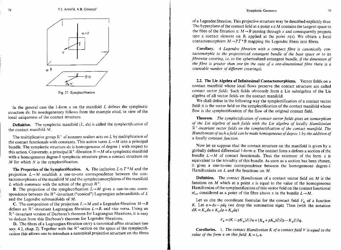
78 V.I. Amol’d, A.B. Givental’
Ci=O II f
V
I
Fig. 27. Symplectification
In the general case the l-form SC on the manifold L defines the symplectic structure dcr. Its nondegeneracy follows from the example cited, in view of the local uniqueness of the contact structure.
Definition. The symplectic manifold (L, da) is called the symplectifcation of the contact manifold M.
The multiplicative group Rx of nonzero scalars acts on L by multiplication of the contact functionals with constants. This action turns L-+ M into a principal bundle. The symplectic structure da is homogeneous of degree 1 with respect to this action. Conversely, a principal tR ’ -fibration N-t M of a symplectic manifold with a homogeneous degree-l symplectic structure gives a contact structure on M for which N is the symplectification.
The Properties of the Symplectification. A. The inclusion L 4 T *M and the projection L+M establish a one-to-one correspondence between the con- tactomorphisms of the manifold M and the symplectomorphisms of the manifold L which commute with the action of the group R ‘.
B. The projection of the symplectification LdM gives a one-to-one corre- spondence between the R ’ -invariant (“conical”) Lagrangian submanifolds of L and the Legendre submanifolds of M.
C. The composition of the projection L+M and a Legendre fibration M-+B defines an R “-invariant Lagrangian fibration L-+B, and vice versa. Using an [w ‘-invariant version of Darboux’s theorem for Lagrangian fibrations, it is easy to deduce from this Darboux’s theorem for Legendre fibrations.
D. The fibres of a Lagrangian fibration carry a canonical affine structure (see sect. 4.2, chap. 2). Together with the RX-action on the space of the symplectifi- cat‘ion this allows one to introduce a canonical projective structure on the fibres
Symplectic Geometry 19
of a Legendre fibration. This projective structure may be described explicitly thus. The hyperplane of the contact field at a point x E M contains the tangent space to the fibre of the fibration z: M-B passing through x and consequently projects into a contact element on B, applied at the point z(x). We obtain a local contactomorphism M-tPT *B mapping the Legendre fibres into fibres.
Corollary. A Legendre fibration with a compact jibre is canonically con- tactomorphic to the projectivized cotangent bundle of the base space or to its jibrewise covering, i.e. to the sphericalized cotangent bundle, if the dimension of the jibre is greater than one (in the case of a one-dimensional jibre there is a countable number of diflerent coverings).
2.2. The Lie Algebra of Infinitesimal Contactomorphisms. Vector fields on a contact manifold whose local flows preserve the contact structure are called contact vector fields. Such fields obviously form a Lie subalgebra of the Lie algebra of all vector fields on the contact manifold.
We shall define in the following way the symplectification of a contact vector field: it is the vector field on the symplectification of the contact manifold whose flow is the symplectification of the flow of the original contact field.
Theorem. The symplectification of contact vectorfields gives an isomorphism of the Lie algebra of such jields with the Lie algebra of locally Hamiltonian R” -invariant vector fields on the symplecti$cation of the contact manifold. The Hamiltonian of such afield can be made homogeneous of degree 1 by the addition of a locally constant function.
Now let us suppose that the contact structure on the manifold is given by a globally defined differential l-form a. The contact form c1 defines a section of the bundle L-M of contact functionals. Thus the existence of the form c1 is equivalent to the triviality of this bundle. As soon as a section has been chosen, it gives a one-to-one correspondence between the homogeneous degree-l Hamiltonians on L and the functions on M.
Definition. The contact Hamiltonian of a contact vector field on M is the function on M which at a point x is equal to the value of the homogeneous Hamiltonian of the symplectification of this vector field on the contact functional cllX, considered as a point of the fibre above x in the bundle L+M.
Let us cite the coordinate formulas for the contact field V, of a function K. Let cr=du--pdq (we drop the summation sign). Then (with the notation dK = K,du + K,dp+ K,dq)
vK =(K -p~,)a/au+ (K, +pK,)aiap- K,aiaq.
Corollaries. 1. The contact Hamiltonian K of a contact field V is equal to the value of the form a on this field: K =&a.

80 V.I. Amol’d, A.B. Givental
2. The correspondence V+-+c( maps the space ofcontactfields bijectively onto the space of smooth functions. In particular, triviality of the bundle L-+M implies the global Hamiltonicity of all RX-invariant locally Hamiltonian fields on L.
The Lie algebra structure introduced in this manner on the space of smooth functions on M is called the Lagrange bracket. The explicit description of this operation looks like this. A contact diffeomorphism, preserving the contact structure, multiplies the form u by an invertible function. Therefore we may associate to a contact Hamiltonian K a new function bK by the rule Lyp = C$~CL. Then the Lagrange bracket [F, G] of two functions will take the form [F, G] = (L,,G - L,,,F + F4, - G4,)/2. With the previous coordinate notations
[F, G]=FG,-FUG-p(F,G,-FUG,)-F,G,+F,G,,
from which, of course, the cited invariant formula for the Lagrange bracket follows. It follows from the intrinsic definition of the Lagrange bracket that the expression on the right-hand side satisfies the Jacobi identity (this is a non- obvious formula).
The Lagrange bracket does not give a Poisson structure ($3, chap. 2), inasmuch as it does not satisfy the Leibniz rule. We shall denote as a Lie structure on a manifold a bilinear operation [ , ] on the space of smooth functions which gives a Lie algebra structure on this space and has the property of localness, i.e. [f, g] lx depends only on the values of the functions A g and of their partial derivatives of arbitrary order at the point x. One can show [42] that a Lie manifold canonically breaks up into smooth symplectic and contact manifolds. This result is a generalization of the theorem on symplectic leaves for Poisson manifolds. The analogues of the other properties of Poisson structures (trans- versal structures, linearization, and the like) for Lie structures have not been studied.
2.3. Contactification. It is defined in the case when a symplectic structure on a manifold N is given as the differential of a l-form 01. By definition the contactification of the manifold (N, ~1) is the manifold IR x N with the contact structure du=cq where u is the coordinate on CR.
Example. Let N be the symplectification of a contact manifold. Since the symplectic structure on N is given as the differential of the canonical l-form CI, the contactification of N is defined. In the special case N = T*B the con- tactification of the manifold N is the space of l-jets of functions on B.
For a given symplectic manifold (N, o) with an exact symplectic structure a different choice of the potential c1 (dcr = CO) leads to different contact structures on R x N. Nevertheless if the difference of two potentials c1i, CQ is exact (al - ~1~ = dd), then the corresponding structures are equivalent in the following sense: the translation (u, x)I+(u+ r+(x), x) is a contactomorphism of (R x N, du-cr,)
Symplectic Geometry 81
onto (R x N, du- a*). If the closed form a, -a2 is not a total differential, then these contact manifolds might not be contactomorphic.
The situation described is typical. The symplectification of contact objects always exists and leads to a topologically trivial symplectic object. The con- tactification exists only under certain conditions of topological triviality and may give a nonunique result. Here is yet another .example of this sort. Let there be given a contactification IF! x N-+N. By a contactification of a Lagrangian manifold A c N is meant a Legendre submanifold LC R x N which projects diffeomorphically onto A. It is not difficult to convince oneself that a contactification of the Lagrangian manifold exists precisely in the case when the closed l-form CIIA on A is exact. If aI,,=d4, then one may set L= {(4(l), ~JE R x N Ii. E A}. The function $I is defined uniquely up to the addition of a locally constant function on A, and we see that the contactification is nonunique. Lagrangian embeddings which admit a contactification will be called exact.
2.4. Lagrangian Embeddings in R’“. An embedded circle in the symplectic plane does not possess a contactification: the integral Ipdq is equal to the area of the region bounded by this circle and is different from zero. In other words, the projection of a Legendre circle in R3 onto the symplectic plane has self-intersection points. The question of the existence of exact Lagrangian embeddings is non-trivial already for the two-dimensional torus.
Theorem ([7]). An orientable compact Lagrangian submanifold in the sym- plectic space R2” has vanishing Euler characteristic.
Proof: The self-intersection number of an orientable submanifold in a tubular neighbourhood of it is the same as in the containing space. The self- intersection number in Euclidean space is zero. The self-intersection number in a tubular neighbourhood is equal to the Euler characteristic of the normal bundle. For a Lagrangian submanifold the normal bundle is isomorphic to the tangent bundle. 0
In particular, the sphere cannot be embedded Lagrangianly in R4. The torus admits Lagrangian embeddings in R4. There exist exact Lagrangian embeddings of the torus in the space R4 with a nonstandard symplectic structure. Exact Lagrangian embeddings of the torus in the standard symplectic space do not exist.
Theorem (M. Gromov, 1984). A closed n-dimensional manifold has no exact Lagrangian embeddings into the standard 2n-dimensional symplectic space.
This theorem, applied to the two-dimensional torus, implies the existence of a symplectic manifold diffeomorphic to R4 but not symplectomorphic to any region in the standard symplectic space R4.
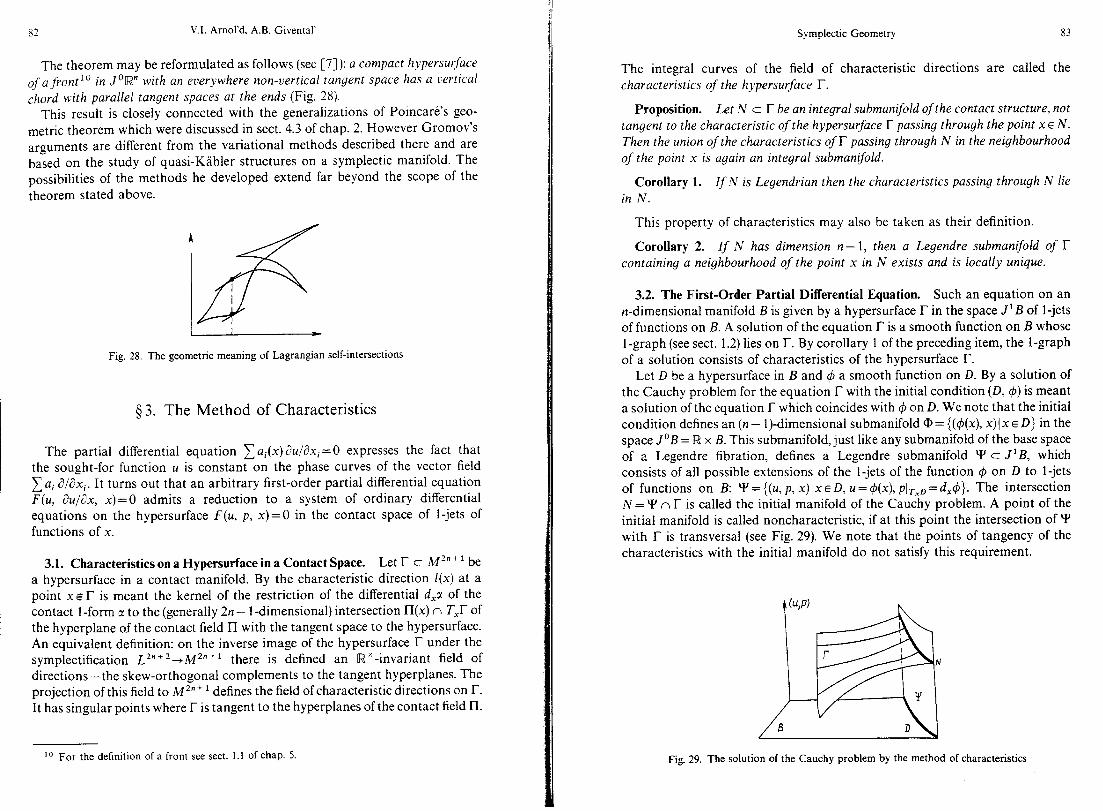
82 V.I. Amol’d. A.B. Givental’
The theorem may be reformulated as follows (see [7]): a compact kypersurfuce of a front lo in J’R” with an everywhere non-vertical tangent space has a vertical chord with parallel tangent spaces at the ends (Fig. 28).
This result is closely connected with the generalizations of Poincare’s geo- metric theorem which were discussed in sect. 4.3 of chap. 2. However Gromov’s arguments are different from the variational methods described there and are based on the study of quasi-Kahler structures on a symplectic manifold. The possibilities of the methods he developed extend far beyond the scope of the theorem stated above.
‘6 Fig. 28. The geometric meaning of Lagrangian self-intersections
$3. The Method of Characteristics
The partial differential equation 1 ai(x)&/~xi=O expresses the fact that the sought-for function u is constant on the phase curves of the vector field c Ui d/ax,. It turns out that an arbitrary first-order partial differential equation F(u, &/ax, x)=0 admits a reduction to a system of ordinary differential equations on the hypersurface F(u, p, x) =0 in the contact space of l-jets of functions of x.
3.1. Characteristics on a Hypersurface in a Contact Space. Let r c M’“+l be a hypersurface in a contact manifold. By the characteristic direction l(x) at a point XET is meant the kernel of the restriction of the differential d,a of the contact l-form ‘1 to the (generally 2n - l-dimensional) intersection II(x) n T,T of the hyperplane of the contact field II with the tangent space to the hypersurface. An equivalent definition: on the inverse image of the hypersurface I- under the symplectification Lzn+ 2 + Mzni ’ there is defined an RX-invariant field of directions-the skew-orthogonal complements to the tangent hyperplanes. The projection of this field to M “+ ’ defines the field of characteristic directions on r. It has singular points where r is tangent to the hyperplanes of the contact field II.
lo For the definition of a front see sect. 1.1 of chap. 5.
Symplectic Geometry 83
The integral curves of the field of characteristic directions are called the characteristics of the kypersurface r.
Proposition. Let N c r be an integral submani$old of the contact structure, not tangent to the characteristic of the kypersurface r passing through the point x E N. Then the union of the characteristics of r passing through N in the neigkbourkood of the point x is again an integral subman$old.
Corollary 1. If N is Legendrian then the characteristics passing through N lie in N.
This property of characteristics may also be taken as their definition.
Corollary 2. If N has dimension n- 1, then a Legendre submanifold of r containing a neigkbourkood of the point x in N exists and is locally unique.
3.2. The First-Order Partial Differential Equation. Such an equation on an n-dimensional manifold B is given by a hypersurface I in the space J’B of l-jets of functions on B. A solution of the equation I is a smooth function on B whose l-graph (see sect. 1.2) lies on r. By corollary 1 of the preceding item, the l-graph of a solution consists of characteristics of the hypersurface I-.
Let D be a hypersurface in B and 4 a smooth function on D. By a solution of the Cauchy problem for the equation r with the initial condition (D, 4) is meant a solution of the equation I- which coincides with 4 on D. We note that the initial condition defines an (n - 1)-dimensional submanifold Q = ((4(x), x)1x E Dj in the space JOB = R x B. This submanifold, just like any submanifold of the base space of a Legendre fibration, defines a Legendre submanifold ‘I-’ c J’B, which consists of all possible extensions of the l-jets of the function 4 on D to l-jets of functions on B: Y = ((u, p, x) Ix E D, u = 4(x), pjT,o = d,4}. The intersection N = ‘I’ n I is called the initial manifold of the Cauchy problem. A point of the initial manifold is called noncharacteristic, if at this point the intersection of Y with r is transversal (see Fig. 29). We note that the points of tangency of the characteristics with the initial manifold do not satisfy this requirement.
Fig. 29. The solution of the Cauchy problem by the method of characteristics

84 V.I. Amol’d, A.B. Givental’
Theorem. A solution of the Cauchy problem in the neighbourhood of a noncharacteristic point of the initial manifold exists and is locally unique.
The l-graph of the solution consists of the characteristics which intersect the initial manifold in a neighbourhood of this point.
Coordinate Formulas. Let r c J ‘(KY’) be given by the equation F(u, p, x) ~0. Then the equation of the characteristics has the form
i=F,.,, @= -F,-pF,, z.i=pF,.
Noncharacteristicity of a point (u, p, x) of the initial manifold is equivalent to the condition that the vector F,(u, p, x) not be tangent to D at the point x. In other words, noncharacteristicity permits one to find from the equation the derivative of the desired function at the points of D along the normal to D, after the derivatives in the tangent directions and the value of the function have been determined by the initial condition 4.
3.3. Geometrical Optics. The equivalence well-known in geometric optics of descriptions of the propagation of light in terms of rays and of fronts served as the prototype of the method of characteristics. The movement of “light cor- pustules” along straight lines in 52” is described by the Hamiltonian H(p, q) =p’. The eikonal equation (8u/3q)2 = 1 describes the propagation of short light waves: the solution of it equal to zero on a hypersurface D in R” is the optical length of the shortest path from the light source D to the point q. The projections to KY of the characteristics composing the l-graph of the function u are the normal lines (rays) to the level surfaces of the function u (the fronts).
@B D a
b
Fig. 30. The fronts (a) and the caustic (b) of an elliptical source
Symplectic Geometry 85
The solutions of the eikonal equation may be many-valued, and the fronts may have singularities. For example, upon propagation of light inside an elliptical source on the plane the front acquires semicubical cusp points (Fig. 30a). Upon movement of the front its singularities slide along a caustic (Fig. 30b). The caustic may be defined as the set of the centres of curvature of the source or as the envelope of the family of rays. In the neighbourhood of the caustic the light becomes concentrated. Singularities of wave fronts and caustics will be studied in chap. 5.
3.4. The Hamilton-Jacobi Equation. A Hamilton-Jacobi equation is an equation of the form H(&/~x, x)=0. It differs from the general first-order equation in that it does not contain the required function u explicitly. Integration of the equations of the characteristics reduces essentially to the integration of the Hamiltonian system with Hamiltonian H(p, q). The eikonal equation is a special case of the Hamilton-Jacobi equation.
The path, inverse to the method of characteristics, of integration of Hamilton- ian systems by a reduction to the solution of a Hamilton-Jacobi equation has proved to be very effective in mechanics.
Jacobi’s Theorem. Let u(Q, q) be a solution of the Hamilton-Jacobi equation H(au/aq, q)= h depending on n parameters Q=(h, ;1,, . . . , &-l) and on the n variables q. Let us suppose that the equation au(Q, q)/aq =p is solvable for Q, in particular, that det(a2u/aqaQ)#0. Then the functions Q(p, q) are n involutivejrst integrals of the Hamiltonian H.
Indeed, the Lagrangian manifolds Aa with the generating functions uTQ, .), ~~=((~,q)~p=au(e,q)iaq}, are the fibres of a Lagrangian fibration over the space of parameters Q. The Hamilton-Jacobi equation means that the restriction of H onto A, is equal to h, i.e. that the Hamiltonian of the system is a function of Q. 0
Success in applying Jacobi’s theorem is always tied up with a felicitous choice of the system of coordinates in which the separation of the variables in the Hamilton-Jacobi equation takes place. It was by just such a method that Jacobi integrated the equation of the geodesics on a triaxial ellipsoid. One says that in the equation H(au/aq, q)= h the variable q1 is separable, if du/aq, and q1 enter into H only in the form of a combination 4(au/aq,, ql). Then, in trying to find a solution in the form u=ul(ql)+ U(q,, . . , q.), we arrive at the system ~(au/aq,,q,)=i.,, H@,, au/aq,,. ..,au/aq,,q,,. . ., q.)=h. If in the second equation variables again separate etc., then we finally arrive at a solution of the original equation of the form ul(ql, &)+u,(q,, I.,, E.2)+ _ . . +u,(q,, 11,. . . , jun-l, h) and we shall be able to apply Jacobi’s theorem.
Let us illustrate this approach with the example of Euler’s problem of the attraction of a point on the plane by two fixed centres. Let rl, r2 be the distance from the moving point to the centres O,, O2 (Fig. 31). The Hamiltonian of the

I 86 V.I. Amol’d, A.B. Givental
Fig. 31. Integration of the Euler problem
problem has the form (~2 +~$/2--k(l/r, + 1/r2). Let us pass over to elliptical coordinates (SC, ye) on the plane: 5 =I~ + r2, yl =rI -r2. The level lines of the functions c, ye are mutually orthogonal families of curves--ellipses and hyper- bolas with the foci O,, 0,. In the canonical coordinates ( ps, ptl, 5, I?) on T*Iw2 the Hamiltonian (after some computations) takes on the form
2 52-4c2 H=2p, 52-vr2 --+2p:
4c2-rf2 4k5 52 -___
52-$’
In the Hamilton-Jacobi equation
(a~/a~)~(~~-4~~)+(&+3y1)~(4c~-yl~)=h(5~ -q2)+2kSI
we may separate the variables, setting
(&+?~)2(~2-4c2)-2k~-h~2=i.
I (aU/aYf)‘(4C2 - q2) + hYf2 = - 2
From this we find a two-parameter family of solutions of the Hamilton-Jacobi equation in the form
The endeavour to extract explicit expressions for the trajectories of Hamilton- ian systems from a similar kind of formulas led Jacobi to the problem of the inversion of hyperelliptic integrals, whose successful solution constitutes today one of the best achievements of algebraic geometry.
Symplectic Geometry 87
Chapter 5
Lagrangian and Legendre Singularities
In this section we set forth the foundations of the mathematical theory of caustics and wave fronts. The classification of their singularities is connected with the classification of regular polyhedra. The proofs take contributions from the theory of critical points of functions, from reflection groups, and from Lie groups and Lie algebras. Perhaps this explains why the final results, elementary in their form, were not already obtained in the last century.
4 1. Lagrangian and Legendre Mappings
These are constructions which formalize in the language of symplectic geometry the concepts of a caustic and of a wave front of geometrical optics.
1.1. Fronts and Legendre Mappings. A Legendre mapping is a diagram consisting of an embedding of a smooth manifold as a Legendre submanifold in the total space of a Legendre fibration, and the projection of the total space of the Legendre fibration onto the base. By abuse of language we shall call the composition of these maps the Legendre mapping, too. The image of a Legendre mapping is called its front.
Examples. A. The equidistant mapping is the mapping which associates to each point of an oriented hypersurface in Euclidean space the end point of the unit vector of the normal at this point. The image of the equidistant mapping is called the equidistant (compare sect. 3.3, chap. 4). More generally, let B be a Riemannian manifold and X c B a smooth submanifold. The flow of the contact Hamiltonian H =.IIpll in the contact space ST*B of transversally oriented contact elements moves (in time t) the Legendre submanifold A, of elements tangent to X into a Legendre submanifold A,. The projection of At to the base space B is an equidistant of the submanifold X-the set of free ends of segments of geodesics (extremals of the Lagrangian 11 p Ij ) of length r sent out from X along normals. Thus, the equidistant mapping is Legendrian and the equidistant is its front.
B. Projective duality. The tangential mapping is the mapping which associates to each point of a hypersurface in a projective space the hyperplane tangent at this point. Let us consider in the product IP x P* of the projective space and its dual the submanifold F of pairs (p, p*) satisfyin, 0 the incidence condition: the

88 V.I. Arnol’d, A.B. Givental
point p E P lies in the hyperplane p * c P, and also the submanifold F* picked out by the dual condition: the point p* E P* lies in the hyperplane p c P*.
1 O. The two incidence conditions coincide: F * = F. The projection F + IFP (F * -+ P*) is a Legendre fibration of the manifold of
contact elements F=PT*lQ(F*=PT*P* respectively). 2”. The two contact structures on F = F* coincide. This follows from 1’ and the definition of the contact structure on PT*B. 0
The tangential mapping is just the projection of the Legendre submanifold A of PT*P, formed by the contact elements of the submanifold X of P, to the base
* space of the second Legendre fibration PT [FD *-+I!+*. Therefore the tangential mapping of a smooth hypersurface is Legendrian. Its front X* in P* is called the dual hypersur ace.
f 3”. The Leendre submanifolds A and A* coincide (Fig. 32).
PJ*tP = PT”IP*
p\
lP=JX x*clp*
Fig. 32. Projective duality
Indeed, a Legendre manifold is determined by its projection to the base space of a Legendre fibration.
Corollary. (X*)* = X.
C. The Legendre transformation. Let us consider the two Legendre fibrations of the standard contact space R2”+ ’ of 1 -jets of functions on KY: (24, p, q) H (24, q)
and (u, P, d - ( pq - u, P). The projection of the l-graph of a function u = S(q) onto the base of the second
fibration gives a Legendre mapping q ~(qaS/8q-S(q), dS/cYq). In the case that the function S is convex, the front of this mapping is again the graph of a convex function u= S*(p)--the Legendre transform of the function S (compare sect. 1.2, chap. 3).
The fronts of Legendre mappings are in general not smooth. The problem of classifying the singularities of fronts reduces to the study of Legendre singular- ities (i.e. singularities of Legendre mappings). Generic Legendre singularities are different from the singularities of generic mappings of n-dimensional manifolds into n + l-dimensional ones. Thus the projection of a generic space curve into the plane has as its singularities only self-intersection points, while the projection of a generic Legendre curve in a Legendre fibration has cusp points as well.
Symplectic Geometry 89
By a Legendre equivalence of two Legendre mappings is meant a con- tactomorphism of the corresponding Legendre fibrations which takes the Legendre manifold of the first Legendre mapping over into the Legendre manifold of the second.
Remarks. 1. A contactomorphism of Legendre fibrations is uniquely deter- mined by a diffeomorphism of the base spaces. A smooth front of a Legendre mapping uniquely determines the original Legendre s.ubmanifold. In this sense the effect of a Legendre equivalence is reduced to the effect of the diffeomorphism of the base on the front. This remark is also applicable to singular fronts whose set of points of regularity is dense in the original Legendre manifold. The last condition is violated only for germs of Legendre mappings forming a set of infinite codimension in the space of all germs.
2. One can show that (up to equivalence) all Legendre singularities can already be realized in the case of equidistants of hypersurfaces in Euclidean space. In this sense the investigation of Legendre singularities coincides with the investigation of equidistants (one can show that to nearby Legendre singularities correspond equidistants of nearby hypersurfaces and conversely, so that the generic singularities for fronts of Legendre mappings are the same as for equidistants), The same may be asserted for the singularities of hypersurfaces projectively dual to smooth ones, or for the singularities of Legendre transforms of graphs of smooth functions.
1.2. Generating Families of Hypersurfaces. A nonsingular Legendre map- ping is determined by its front-the generating hypersurface of the Legendre manifold. An arbitrary Legendre mapping can be given by a generating family of hypersurfaces. Let us consider an auxiliary trivial fibration Rk+‘+R’ of a “big space” Rk +’ over the base space R’. The contact elements in Rk+’ which are tangent to the fibres of the fibration form the mixed submanifold P c PT* I&!‘+’ of codimension k. The mixed manifold is fibred over the manifold of contact elements of the base space (Fig. 33). A Legendre submanifold of PT*pk+’ is called regular if it is transversal to the mixed space P.
Lemma. 1. The image of the projection of the intersection of a regular Legendre manifold with the mixed space P into the space of contact elements of the base is an immersed Legendre submanifold.
2. Every germ of a Legendre submani$old of PT*[w’ can be obtained by this construction from some regular Legendre submanifold, generated by a generating hypersurface, of a suitable auxiliary fibration.
Let us give the proof of the second assertion of the lemma. In the fibra- tion PT* R’+ R’ let us introduce contact Darboux coordinates (u, p, q)= (u,p,, pJ, q,, q5), IuJ=(l,. . . , l-l], InJ=@, so that the Legendre sub- manifold germ being investigated projects injectively to the space of the coordinates (p,, ql) along the (u, p1, q,)-space. Then from the relations

90 V.I. Amol’d, A.B. Givental’
Fig. 33. The mixed space
du =pdq =d(p,q,) - q,dp, +p,dq, we get: there exists a germ of a smooth function S(p,, qr) so that our Legendre submanifold is given by the equations
PI = as/$!,, qJ = - ~Sh%J, u = PJqJ + s(pJ, 4,).
Now let us consider the hypersurface U= F(x, q) in the “big” space lRk+‘, where k= JJI and F(x, q)=xq,+S(x, q,), as the generating hypersurface of the Legendre manifold u= F, y= F,, p= F,. An application of the construction of the first part of the lemma leads to the original Legendre germ in PT*R’. The regularity condition has the form det( Fsq,) # 0 and is fulfilled. 0
The hypersurface of the big space, through which the germ of the Legendre mapping is given by the construction described in the lemma, is called a generatingfamily ofhypersurfuces of this Legendre mapping (the elements of the family are in general singular intersections of the hypersurface with the fibres of the fibration Rk + I+ 52).
Remark. The “physical meaning” of the generating family consists in the following. Let us consider the propagation of light in R’ from a source X c R’ of dimension k. According to Huygens’ principle, each point x of the source radiates a spherical wave. Let us denote by F(x, q) the propagation time of this wave to the point q of the space R’. Then the condition that the least time of motion of the light from the source X to the point q is equal to u gives the equations:
3x E X: u = F(x, q), ~F(x, q)/ax = 0. (1)
But this is just the equation of the front for the projection to R’ of the intersection of the Legendre manifold (u=F, y= F,, p=F,) with the mixed space {y=O}.
By a fibred equivalence of generating families of hypersurfaces l-r and Tz in the total space of the fibration R k+‘+R’ is meant a fibred diffeomorphism (x, q)++(h(x, q), 4(q)) which transfers I-r into Tz. Let I-c M be a smooth hypersurface with a simple equation f=O. The doubling of M with branching along T is the hypersurface in the direct product Rx M with the equation u’=f(u), UER. In the complex case the doubling is a double covering of M
Symplectic Geometry 91
ramified along T. The real type of the equation depends on the choice of the side of T. Two families of hypersurfaces in auxiliary fibrations with a common base space are called stably fibred-equivalent if they become fibred-equivalent after a series of fibrewise doublings.
Theorem ([S]). Two germs of generating families of hypersurfaces give equitl- alent germs of Legendre mappings ifand only ifthesefamilies of hypersurfuces are jibred stably equicalent.
The reason for the appearance of stable equivalence here will become clear in 42.
1.3. Caustics and Lagrangian Mappings. A Lagranyian mapping is a diagram consisting of an embedding of a smooth manifold as a Lagrangian submanifold in the total space of a Lagrangian fibration and the projection to the base space of this fibration.
Examples. A. A gradient mapping q~c?S/Zq is Lagrangian.
B. The Gauss mapping of a transversally oriented hypersurface in Euclidean space R” to the unit sphere is Lagrangian. In fact, it is a composition of two maps. The first associates to a point of the hypersurface the oriented normal to the hypersurface at that point; its image is a Lagrangian submanifold in the space of all straight lines in R”, which is isomorphic to the (co)tangent bundle of the sphere (Fig. 34). The second is the Lagrangian projection T*S”- ’ -+S’- ‘.
/ / 02;:\. \ / r” \ Fig. 34. The Gauss mapping is Lagrangian
C. The normal mapping, which associates to a vector sof a normal to a submanifold in Euclidean space, applied at the point u, the point u of the space itself, is Lagrangian.
The set of critical values of a Lagrangian mapping is called a caustic (Fig. 35).
Example. The caustic of the normal mapping of a submanifold in Euclidean space is the set of its centres of curvature: to construct the caustic, one must lay out along each normal the respective radii of the principal curvatures.

92 V.I. Arnol’d, A.B. Givental’
Fig. 35. The caustic of a Lagranglan mapping
A Lagrangian equivalence of Lagrangian mappings is a symplectomorphism of the Lagrangian fibrations which takes the Lagrangian manifold of the first mapping over into the Lagrangian manifold of the second.
Remarks. 1. An automorphism of the Lagrangian bundle T*M + M factors into the product of an automorphism induced by a diffeomorphism of the base space and a translation automorphism (p, q)w(p + 4(q), q), where 4 is a closed l-form on M.
2. The caustics of equivalent Lagrangian mappings are diffeomorphic. The converse is in general not true.
3. Every germ of a Lagrangian mapping is equivalent to a germ ofa gradient (Gauss, normal) mapping. All germs of Lagrangian mappings which are close to a given gradient (Gauss, normal) mapping are themselves gradient (Gauss, normal). Therefore the generic local phenomena in these classes of Lagrangian mappings are the same as in the class of all Lagrangian mappings.
1.4. Generating Families of Functions. A Lagrangian section of a cotangent bundle, i.e. a closed l-form on the base space, is given by its generating function-a potential of this l-form. Let us consider an auxiliary fibration iWk+‘+R1. The covectors in T*IWk+’ which vanish on the tangent space to the fibre at their point of application form the mixed submanifold Q t T*[Wk+‘. The mixed manifold is fibred over T*Iw’ with k-dimensional isotropic fibres. A Lagrangian submanifold of T * iw k+l transversal to Q is called regular. The projection to T*Lw’ of the intersection An Q of a regular Lagrangian manifold is an immersed Lagrangian submanifold in T*Lw’. Conversely, any germ of a Lagrangian submanifold of T*Iw’ can be obtained as a projection of the intersection with the mixed submanifold Q of a regular Lagrangian submanifold A which is a section of the cotangent bundle of the “big space”, for a suitable choice of the auxiliary fibration.
A generatingfamily offunctions of a germ of a Lagrangian mapping is a germ of a function on a “big” space which generates a regular Lagrangian section of the cotangent bundle of the “big” space and by means of the construction described above defines the given Lagrangian mapping. (The function on [Wk+’ is here
Symplectic Geometry 93
regarded as a family of functions on the fibres of the projection [Wk+‘+(W1, depending on the point of the base space as a parameter).
In Darboux coordinates (pr, pJ, ql, qr) for the Lagrangian fibration T*[w*-, (w’ such that the Lagrangian submanifold of T*[w’ projects nonsingularly along the (pI, q,)-space, let us give this submanifold by the equations p,=&Y/aq,, qJ= -%/ap,, where S(p,, qr) is some smooth function. Then the family of functions F(x, q)=xq, +S(x, ql) may be taken as a generating family of the Lagrangian mapping of our Lagrangian submanifold of T*Lw’ to the base space IR’.
In the general case the family of functions F(x, q) is generating for some Lagrangian mapping if and only if rk(F,.,, FXq)= k. In this case it defines
a) a regular Lagrangian submanifold A in T*[Wk+‘:
b) the intersection of A with the mixed space Q= (y=O}:
AnQ={(p, x, dlF,=O, P=F,};
c) a Lagrangian submanifold L c T*IW’--the projection of An Q:
L=C(p, 4)13x: FAX, 4)=Q P=Fqk 4));
d) the caustic K in IP:
K=(qI3x:F,(x,q)=O,detIF,,(x,q)l=O}; (2) We shall call two families of functions F, (x, q), F, (x, q) fibred R +-equivalent if
there exists a fibred diffeomorphism (x, q) H (h(x, q), 4(q)) and a smooth function Y(q) on the base space, such that F,(x, q) = F,(h(x, q), 4(q))+ Y(q). Two families of functions F,(x,, q), F,(x,, q), in general of a different number of variables, will be called stably fibred R +-equivalent if they become fibred R+- equivalent after adding to them nondegenerate quadratic forms Q1(z,), Q2(.z2) in new variables
Example: the family x3 +yz +qx (q is the parameter) is stably fibred R+-equivalent to the family x3 + qx.
Theorem ([9]). Two germs of Lagrangian mappings are Lagrangianly equiu- alent if and only if the germs of their generating families are stably fibred R +-equivalent.
1.5. Summary. The investigation of singularities of caustics and wave fronts led to the study of generating families of functions and hypersurfaces. The formulas (1) and (2) mean that the front of a generating family of hypersurfaces consists of those points of the parameter space for which the hypersurface of the family is singular, and the caustic of a generating family of functions consists of
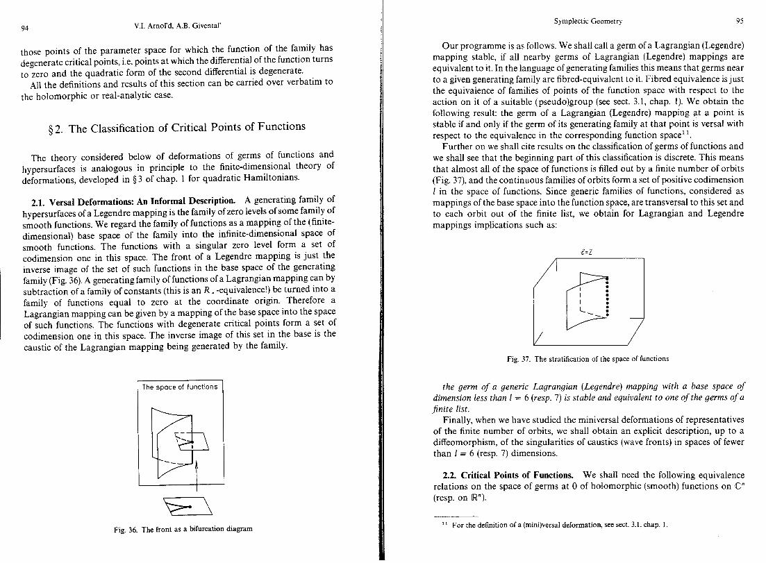
94 V.I. Arnol’d, A.B. Givental’
those points of the parameter space for which the function of the family has degenerate critical points, i.e. points at which the differential of the function turns to zero and the quadratic form of the second differential is degenerate.
All the definitions and results of this section can be carried over verbatim to the holomorphic or real-analytic case.
$2. The Classification of Critical Points of Functions
The theory considered below of deformations of germs of functions and hypersurfaces is analogous in principle to the finite-dimensional theory of deformations, developed in 9 3 of chap. 1 for quadratic Hamiltonians.
2.1. Versa1 Deformations: An Informal Description. A generating family of hypersurfaces of a Legendre mapping is the family of zero levels of some family of smooth functions. We regard the family of functions as a mapping of the (finite- dimensional) base space of the family into the infinite-dimensional space of smooth functions. The functions with a singular zero level form a set of codimension one in this space. The front of a Legendre mapping is just the inverse image of the set of such functions in the base space of the generating family (Fig. 36). A generating family of functions of a Lagrangian mapping can by subtraction of a family of constants (this is an R + -equivalence!) be turned into a family of functions equal to zero at the coordinate origin. Therefore a Lagrangian mapping can be given by a mapping of the base space into the space of such functions. The functions with degenerate critical points form a set of codimension one in this space. The inverse image of this set in the base is the caustic of the Lagrangian mapping being generated by the family.
Fig. 36. The front as a bifurcation diagram
Symplectic Geometry 95
Our programme is as follows. We shall call a germ of a Lagrangian (Legendre) mapping stable, if all nearby germs of Lagrangian (Legendre) mappings are equivalent to it. In the language of generating families this means that germs near to a given generating family are fibred-equivalent to it. Fibred equivalence is just the equivalence of families of points of the function space with respect to the action on it of a suitable (pseudo)group (see sect. 3.1, chap. 1). We obtain the following result: the germ of a Lagrangian (Legendre) mapping at a point is stable if and only if the germ of its generating family at that point is versa1 with respect to the equivalence in the corresponding function space”.
Further on we shall cite results on the classification of germs of functions and we shall see that the beginning part of this classification is discrete. This means that almost all of the space of functions is filled out by a finite number of orbits (Fig. 37), and the continuous families of orbits form a set of positive codimension I in the space of functions. Since generic families of functions, considered as mappings of the base space into the function space, are transversal to this set and to each orbit out of the finite list, we obtain for Lagrangian and Legendre mappings implications such as:
C-2
Fig. 37. The stratification of the space of functions
the germ of a generic Lagrangian (Legendre) mapping with a base space of dimension less than 1 = 6 (resp. 7) is stable and equivalent to one of the germs of a finite list.
Finally, when we have studied the miniversal deformations of representatives of the finite number of orbits, we shall obtain an explicit description, up to a diffeomorphism, of the singularities of caustics (wave fronts) in spaces of fewer than I = 6 (resp. 7) dimensions.
2.2. Critical Points of Functions. We shall need the following equivalence relations on the space of germs at 0 of holomorphic (smooth) functions on @” (resp. on Rn).
I1 For the definition of a (mini)versal deformation, see sect. 3.1, chap. 1.

96 V.I. Amol’d, A.B. Givental’
R-equivalent germs are taken into each other by the germ at 0 of a
diffeomorphism of the preimage space; R.-equivalent germs become R-equivalent after addition of a suitable con-
stant to one of them; V-equivalent germs become R-equivalent after multiplication of one of them
with the germ of a non-vanishing function (V-equivalence of germs of functions is just equivalence of the germs of their zero-level hypersurfaces).
At a critical (or singular) point of a function its differential turns to 0. The critical point is nondegenerate if the quadratic form of the second differential of the function at that point is so. By the Morse lemma [9], in the neighbourhood of a nondegenerate critical point the function is R-equivalent to a function &xff... _ + x,” + const. By the corank of a critical point is meant the corank of the second differential of the function at that point.
The Morse Lemma with Parameters ([S]). The germ of a.finction at a critical
point of corank r is R-equivalent to the germ at 0 of a function of the form const + 4(x,, . . . , x,)~x;+~ f . . _ kx,‘, where ~$=O(\xl~).
This lemma explains the appearance of the concept of stable equivalence in the theorems on generating families: in fact the germ of a Lagrangian (Legendre) mapping at a point may be given by a germ of a generating family with zero second differential of the function at that point. Fibred equivalence of in this sense minimal generating families means the same as the equivalence of the original mappings. For the construction of minimal generating families it is only necessary that in the constructions of sects. 1.2 and 1.4 one choose the number of “pathological” variables p, to be minimal.
Germs of functions (possibly of a different number of variables) are called stably R(R + , V)-equivalent if they are R (R + , V)-equivalent to sums of the same
germ of rank 0 with nondegenerate quadratic forms of the appropriate number of additional variables.
A degenerate critical point falls apart into nondegenerate ones upon deform- ation (Fig. 38). If the number of the latter is finite for an arbitrary small deformation, then the critical point is said to be of finite multiplicity. The germ of a function at a critical point of finite multiplicity is R-equivalent to its Taylor polynomial of sufficiently high order. In the holomorphic case finite multiplicity is equivalent to isolatedness of the critical point. The number of nondegenerate
Fig. 38. Morsification
Symplectic Geometry 97
critical points into which such a point falls apart upon deformation does not depend on the deformation and is called the multiplicity or the Milnor number p of the critical point. The germs of infinite multiplicity form a set of infinite codimension in the space of germs of functions.
2.3. Simple Singularities. A germ of a function at a critical point is called simple if a neighbburhood of it in the space of germs of functions at this point can be covered by a finite number of equivalence classes. The simplicity concept depends in general on the equivalence relation and is applicable to an arbitrary Lie group action on a manifold. The number of parameters (moduli) which are needed for the parametrization of the orbits in the neighbourhood of a given point of the manifold is called the modality of the point. Examples: the modality of an arbitrary quadratic Hamiltonian on iw”’ with respect to the action of the symplectic group is equal to n; the critical value is a modulus with respect to R- equivalence on the space of germs of functions at a given point, but is not a modulus for R.-equivalence on this space.
Theorem ([9]). A germ ofafunction at a critical point, which is simple in the space of germs of smoothfinctions (with value zero at that point), is stably R + (reip. R, V)-equivalent to one of the following germs at zero
AZ&f2 I:f(x)= +x’+‘; D;,pL4:f(x,y)=x2yIfIyP-‘;
Ed : f(x, y) = x3 i y4; E,: f(x, y) = x3+xy3;
E, : f (x, y) = x3 + y5.
The nonsimple germs form a set of codimension 6 in these spaces.
Remarks. 1) The index ,U is equal to the multiplicity of the critical point. 2) The enumerated germs are pairwise stably inequivalent, except for the
following cases: A2:, L A;,‘, A+ : P A;, D+ 2k+l 1 D;k+l, E6’ : E,, A: 5 A; (stably).
3) In the holomorphic case the germs which differ only in the sign f are equivalent among themselves. Figure 39 depicts the adjacencies of the simple classes and the unimodal classes bordering on them in the space of functions.
A,- A,- A,- A,- A 5-A,- A,- A,- ---
D,- D5q,D6\\“,<D8-- ---
E,- E,-- E,
Fig. 39. Adjacencies of simple singularities of functions
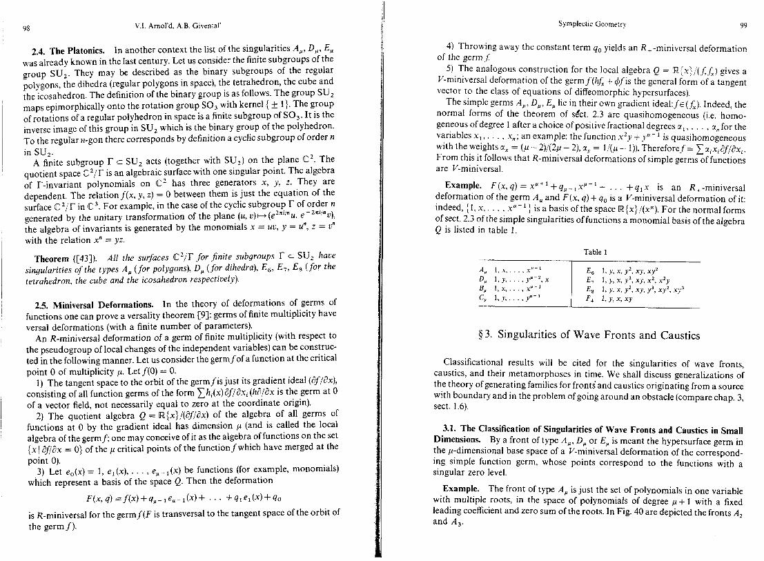
98 V.I. Arnol’d, A.B. Givental
2.4. The Platonic% In another context the list of the singularities A,, D,, E, was already known in the last century. Let us consider the finite subgroups of the group SUP. They may be described as the binary subgroups of the regular polygons, the dihedra (regular polygons in space), the tetrahedron, the cube and the icosahedron. The definition of the binary group is as follows. The group SU2 maps epimorphically onto the rotation group SO3 with kernel .( f l}. The group of rotations of a regular polyhedron in space is a finite subgroup of SO,. It is the inverse image of this group in SU, which is the binary group of the polyhedron. To the regular n-gon there corresponds by definition a cyclic subgroup of order n in SU2.
A finite subgroup I- c SU, acts (together with SU2) on the plane C2. The quotient space rC’/I’ is an algebraic surface with one singular point. The algebra of r-invariant polynomials on Cc 2 has three generators x, y, z. They are dependent. The relationf(x, y, z) = 0 between them is just the equation of the surface cCz/T in C3. For example, in the case of the cyclic subgroup r of order n generated by the unitary transformation of the plane (u, U)H (e2rri’nU, e-2ni’nu), the algebra of invariants is generated by the monomials x = ut’, y = u”, z = U” with the relation xn = yz.
Theorem ([43]). All the surfaces @‘/I- for jinite subgroups r c SU, have singularities ofthe types A,, (for polygons), D, (for dihedra), E,, E,, Es (for the tetrahedron, the cube and the icosahedron respectively).
2.5. Miniversal Deformations. In the theory of deformations of germs of functions one can prove a versality theorem [9]: germs of finite multiplicity have versa1 deformations (with a finite number of parameters).
An R-miniversal deformation of a germ of finite multiplicity (with respect to the pseudogroup of local changes of the independent variables) can be construc- ted in the following manner. Let us consider the germfof a function at the critical point 0 of multiplicity p. Let f(O) = 0.
1) The tangent space to the orbit of the germfis just its gradient ideal (8f/Jx), consisting of all function germs of the form C hi(x) lJJ/8xi (ha/ax is the germ at 0 of a vector field, not necessarily equal to zero at the coordinate origin).
2) The quotient algebra Q = R(x}/(aJ/ax) of the algebra of all germs of functions at 0 by the gradient ideal has dimension p (and is called the local algebra of the germf; one may conceive of it as the algebra of functions on the set {x I &‘dx = 0) of th e p critical points of the functionfwhich have merged at the point 0).
3) Let e,(x) = 1, e,(x), . . . , e,- 1(x) be functions (for example, monomials) which represent a basis of the space Q. Then the deformation
W,d =f(x)+9p-1e,-l(x)+ . . +q1el(4+q0
is R-miniversal for the germf(F is transversal to the tangent space of the orbit of the germ f).
Symplectic Geometry 99
4) Throwing away the constant term q,, yields an R .-miniversal deformation of the germj:
5) The analogous construction for the local algebra Q = R{xJ/(f,f,) gives a V-miniversal deformation of the germf(hf, + 4?fis the general form of a tangent vector to the class of equations of diffeomorphic hypersurfaces).
The simple germs A,, D,, E, lie in their own gradient ideal:fE(fx). Indeed, the normal forms of the theorem of s&t. 2.3 are quasihomogeneous (i.e. homo- geneous of degree 1 after a choice of positive fractional degrees sll, . . , aL, for the variables x1, . , x,; an example: the function x2y +y”-’ is quasihomogeneous with the weights a, = (p - 2)/(2/1- 2), aY = l/(p - 1)). Thereforef = ~~ixi8~/8xi. From this it follows that R-miniversal deformations of simple germs of functions are V-miniversal.
Example. F(x,q) = xP+l +qP-lx”-l + . . . +qlx is an R+-miniversal deformation of the germ A, and F(x, q) + q. is a V-miniversal deformation of it: indeed, { 1, x, . . , x’ - ’ 3 is a basis of the space [w (x} /(xv). For the normal forms of sect. 2.3 of the simple singularities of functions a monomial basis of the algebra Q is listed in table 1.
Table 1
~
$3. Singularities of Wave Fronts and Caustics
Classificational results will be cited for the singularities of wave fronts, caustics, and their metamorphoses in time. We shall discuss generalizations of the theory ofgenerating families for fronts’and caustics originating from a source with boundary and in the problem of going around an obstacle (compare chap. 3, sect. 1.6).
3.1. The Classification of Singularities of Wave Fronts and Caustics in Small Dimensions. By a front of type A,, D, or E, is meant the hypersurface germ in the p-dimensional base space of a V-miniversal deformation of the correspond- ing simple function germ, whose points correspond to the functions with a singular zero level.
Example. The front of type A, is just the set of polynomials in one variable with multiple roots, in the space of polynomials of degree ,u+ I with a fixed leading coefficient and zero sum of the roots. In Fig. 40 are depicted the fronts A, and A,.

V.I. Arnol’d, A.B. Givental
Fig. 40. Singularities of wave fronts
~ Theorem. A generic wave front in a space of 116 dimensions is stable and in
the neighbourhood of any of its points is diffeomorphic to the Cartesian product of a front of type A,, D,, E, with p 5 I and a nonsingular manifold of dimension 1 -p, or to a union of such fronts which are transversal (Fig. 41).
______ F--.--- --_\ I \\
Q@
I ’ ‘Y i ‘\ ‘\ __
Fig. 41. Transversal fronts (caustics)
* By a caustic of type A, , 0: , Ez is meant the hypersurface germ in the p - l- dimensional base space of an R+- miniversal deformation of the corresponding simple function germ, whose points correspond to the functions with degenerate critical points (i.e. the projection of the cuspidal edge A, of the front of the same name to the base space of the R+-miniversal deformation).
Example. The caustic of type A, is diffeomorphic to the front of type A, - 1 : to a point of this caustic corresponds a polynomial of degree p + 1, whose derivative (i.e. a polynomial of degree p) has a multiple root.
Theorem. A generic caustic in a space of 1 I 5 dimensions is stable and in the neighbourhood of any of its points is diffeomorphic to the Cartesian product of a
Symplectic Geometry 101
caustic of type A,,, D,, E, with .a- 1 I 1 and a nonsingular manifold of dimension 1 -p+ 1, or to a union of such caustics which are transversal.
In particular, a generic caustic in space is locally diffeomorphic to one of the surfaces of Figs. 41,42.
Swallowtai I Pyramid Purse (elliptic umbtlic) (hyperbolic umbllic J
Fig. 42. Singularities of caustics in OX3
Fronts and caustics of type A,, D,, E, are stable in all dimensions. Generic fronts (caustics) in spaces of dimension I2 7 (12 6) may be unstable12. This is connected with the existence of nonsimple singularities of functions, the first of which is P, (see Fig. 39). The existing classification of unimodal and bimodal critical points of functions [9] carries considerable information about the singularities of generic fronts (caustics) in spaces of I < 11 (I I 10) dimensions. Nonetheless a classification of the singularities of generic caustics in iw6, even only up to homeomorphisms, is lacking for the present.
3.2. Boundary Singularities. Let us suppose that the source of a radiation is a manifold with boundary (for example, the solar disk). In this situation the wave front has two components-the front of the radiation of the boundary and the front from the source proper (Fig. 43). The caustic in this case has three components in general-the boundaries of light and umbra, umbra and penumbra, and also of penumbra and light.
The corresponding theory of Lagrangian and Legendre mappings and their generating families leads to the theory of singularities of functions on a manifold with boundary. A boundary should be taken to mean a nonsingular hypersurface on a manifold without boundary. A point is considered singular for a function on the manifold with boundary if it is critical either for the function itself or for its restriction to the boundary. The diffeomorphisms which enter into the definition of equivalence are required to preserve the boundary (in the real case, each half- space of the complement of the boundary). The theory of boundary singularities of functions includes the usual one, since the functions may have singularities also outside the boundary.
I2 and for 12 10 (I 2 6) they may have functional moduli.

102 V.I. Arnol’d, A.B. Givental’
Fig. 43. A source with a boundary
Theorem. The simple germs of functions on a manifold with boundary are stably equivalent to the germs at 0 (the boundary is x = 0) either of 2: (*', a: (", id (?): 2 x + f (y, z), where f (y, z) is the germ Ai, 02, E: of sect. 2.3 on the boundary;orofB:,a22:~xP;CZ,a>2:xy+yP;F~:+x2+y3.
Remarks. 1) The germs enumerated are pairwise inequivalent, except for the
cases: A:, L A,, C: E B: (stably), but also, germs which differ in the signs + are equivalent in the holomorphic and V-classification, except for the case C 2k+ i, in which the hypersurfaces Czk+ i are real-inequivalent.
2) The role of the nondegenerate singularities is played in the theory with boundary by the germs 2,: +x&y:* . . . ky,’ and A,: ~(x-x~)~ +y: * . . +y;, so that the singularities Ap, 6,, I!?, may be considered as the stabilizations of the A,, D,, E, singularities on the boundary.
3) The simple singularities outside the boundary are Ad, 02, Et. 4) The theory of boundary singularities is equivalent to the theory of critical
points of functions which are even in the variable u on the double covering x = u’, ramified along the boundary x = 0.
The construction of miniversal deformations of boundary singularities of finite multiplicity is analogous to that described in sect. 2.6 and reduces to finding a monomial basis of the local algebra R(x, y,, . . . , y,)/(xaf/ax, aflay). For the germs B,, C,, F, such a basis is indicated in table 1. The fronts of the miniversal families of B, and C, are diffeomorphic to each other and consist of two irreducible hypersurfaces in the space of polynomials of degree p with a fixed leading coefficient-the set of polynomials with a zero root and the set of polynomials with a multiple root. In the case of B, the first component has the meaning of the front of the radiation from the boundary of the source (A”,), the second that of the front of the source itself (A i), but in the case of C, everything is the other way around. The caustics of B, and C, are diffeomorphic to the fronts of B,+1 and C,,,. The fronts and the caustics of the germs Alp, 6,,, E, are the same as for A,, D,, E,. Figure 44 depicts the caustics of B,, C,, F, in space and on the plane.
Symplectic Geometry 103
Fig. 44. Boundary caustics
Theorem. A germ of a generic wave front (caustic) from a “source with boundary” in a space of 1 I 4 (1 I 3) dimensions is stable and is difleomorphic to the Cartesian product of the front (caustic) of a miniversal family of one of the germs A,, B,, C,, D,, E,, F, with p _< 1 (,u-- 1 I 1) and a germ of a nonsingular manifold of dimension 1 -,u (1-p + l), or to a union of such fronts (caustics) which are transversal. Unstable generic fronts (caustics) are encountered in spaces of dimension 12 5 (12 4).

104 V.I. Arnol’d, A.B. Givental’
Example([64]). In Euclidean space R3 let there be given a generic surface with boundary. Where the boundary is tangent to a line of curvature of the surface, three things together-the focal points of the surface (A,), the focal points of the boundary (Jz), the normals to the surface at the points of the boundary (B,)-form the caustic F, at the centre of curvature of the surface.
The symplectic version of the theory of caustics from a source with boundary leads to the following object: in the total space of a Lagrangian fibration, two nontangent Lagrangian manifolds which intersect along a hypersurface of each of them. The caustic of such an object consists of three parts: the caustics of both Lagrangian manifolds and the projection of their intersection to the base space of the Lagrangian fibration.
The theory of generating families of such objects reduces to the theory of singularities of functions on a manifold with boundary [SS]. Interchanging the two Lagrangian manifolds corresponds to interchanging the stable equivalence classes of the function itself and its restriction to the boundary [65]. This duality generalizes the duality of the B and C series of simple boundary singularities and clears up the classification of unimodal and bimodal critical points of functions on a manifold with boundary [53].
3.3. Weyl Groups and Simple Fronts. The classification of simple germs of functions on a manifold with boundary is parallel to many other classifications of “simple” objects. One of them is the classification of symmetry groups of regular integral polyhedra in multidimensional spaces.
A Weyl group is a finite group of orthogonal transformations of a Euclidean space V which is generated by reflections in hyperplanes and preserves some full- dimensional integral lattice in V. The irreducible pairs (Weyl group, lattice) are classified by Dynkin diagrams [14]; see Fig. 45.
The vertices of the Dynkin diagram correspond to the basis vectors of the lattice Z”, the edges give the scalar product of the basis vectors according to a definite rule (the absence of an edge signifies their orthogonality). The Weyl group corresponding to the diagram is generated by the reflections in the
E6 --I-- A/, - --- -
BpA a+-+- ---- E7 -T--
c, c+b-o- - - - e E8 --I----
D,,, >---e Fc a 52 0~0
Fig. 45. Dynkin diagrams
Symplectic Geometry 105
hyperplanes orthogonal to the basis vectors of the lattice. Any Weyl group is isomorphic to a direct product of irreducible ones.
Examples. The Weyl group A i is just the group Z2, which acts by reflection on the line. The Weyl groups on the plane (besides A i 0 A,) are just the symmetry groups of the regular triangle, square and hexagon (Fig. 46). To the diagram C, corresponds the symmetry group of the p-dimensional cube, and to B, that of its dual, the p-dimensional “octahedron”, so that the corresponding Weyl groups coincide, but the lattices connected with them are different.
A, - 0,= c, +=o
Fig. 46. Weyl groups on R2
Let us consider the action of a Weyl group W on the complexified p- dimensional space Vc. It turns out that the quotient manifold VC/W is nonsingular and diffeomorphic to Q’.
Example. For the group A, of permutations of the roots of a polynomial of degree p + 1 (with zero root sum) this is a fundamental theorem about symmetric polynomials: every symmetric polynomial can be uniquely represented as a polynomial in the elementary symmetric functions.
Let us consider all reflections in hyperplanes (mirrors) which lie in the Weyl group W. The image of the mirrors under the projection Vc + Vc/ W (the Vieta map) is a singular hypersurface and is called the discriminant of the Weyl group.
Example. The discriminant of the Weyl group A, is the variety of poly- nomials with multiple roots in the p-dimensional space of polynomials of degree p + 1 in one variable with a given leading coefficient and zero sum of the roots.
Theorem. The complex front of a simple boundary germ is diffeomorphic to the discriminant of the irreducible Weyl group of the same name.
Corollary. The strata of the complex front of a simple boundary germ are in one-to-one correspondence with the subdiagrams of the corresponding Dynkin diagram (a subdiagram is obtained by discarding a certain number of vertices of the diagram together with the edges adjoining them, Fig. 47).

106 V.I. Amol’d, A.B. Givental’ Symplectic Geometry 107
f43 3A1 0 0 0
0 AI
Fig. 47. The stratification of the front D,
Remarks. 1) The singularity with the front G, can be obtained as a simple singularity in the theory of functions on the plane invariant with respect to the symmetry group of a regular triangle.
2) Besides Weyl groups, platonics, fronts and caustics other objects too can be classified by Dynkin diagrams, for example, complex simple Lie groups [24]. We have already pointed out this connection in chap. 1, sect. 4.3 with regard to the example of the symplectic group Sp(2~ @)--it corresponds to the diagram C,. Direct correspondences between the various such classifications have not been established completely, although many of them are known. Thus, from a simple complex Lie algebra one can construct a simple singularity of surfaces in C3 together with its miniversal deformation [15]. The general reason for the universality of the A, B, C, D, E, F, G-classification remains rather mysterious.
3.4. Metamorphoses of Wave Fronts and Caustics. A spreading wave front will not at all moments of time be a generic front: at isolated moments of time it bifurcates. The investigation of such metamorphoses leads to the problem of generic singularities in a family of Legendre mappings.
Let us consider a family of Legendre mappings depending on one parameter t-the time. We shall call the union in space-time (the product of the base space by the time axis) of the fronts corresponding to the different values of t the big front.
Lemma. The germ of the big front at each point is a germ of a front of a Legendre mapping in space-time.
Indeed, it is given by the generating family FJx, 4) = 0 of hypersurfaces in the x-space with the (4, t)-space-time as the base space. 0
An equivalence of metamorphoses of fronts is just a diffeomorphism of space- time which takes the big fronts over into each other and preserves the time function on this space up to an additive constant: t H t + const.
Example. Special metamorphoses. In the space R”’ x [w’ let us consider a big front C which is the product of R” with the front of a simple germ of multiplicity p. Let us choose as a miniversal deformation of the simple germ f a monomial deformation of the form f(x)+qOePmI(x)+. . . +qP-2e,(x)+q,-,, where e, _ I (x) represents the class of the highest quasihomogeneous degree in the local algebra of the germ (for example, for A, : x’+ ’ + qOxP-’ + . . . + qP- 1 ). Let us denote by (ri, . . _ , 7,) the coordinates on R” and let us give a special metamorphosis by a time function on R” x II%@ of the form t = 5 qO rh T! & . . . *7: or t=r,.
Theorem. The metamorphoses in generic one-parameter families of fronts in spaces of dimension 1 < 6 are locally equivalent to the germs of special meta- morphoses at 0, where ,a+m = I+ 1 (Fig. 48).
AZ A2 A3
Fig. 48. Metamorphoses of wave fronts
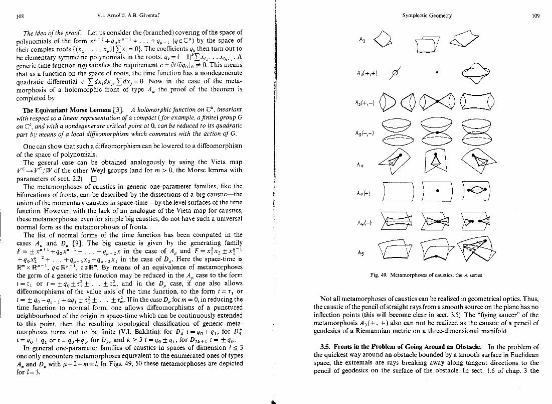
108 V.I. Arnol’d. A.B. Givental
The idea ofthe proof: Let us consider the (branched) covering of the space of polynomials of the form x”+ ’ + q,x “-‘+. . . +qp-1 (q~@‘) by the space of their complex roots ((x,, . . . , x~) 1 xxi = O}. The coefficients qk then turn out to be elementary symmetric polynomials in the roots: qk = (- l)kx~i,. . . xik+, . A generic time function t(q) satisfies the requirement c = &/dq, 1 0 # 0. This means that as a function on the space of roots, the time function has a nondegenerate quadratic differential c.xdxidxj, xdxj = 0. Now in the case of the meta- morphosis of a holomorphic front of type A, the proof of the theorem is completed by
The Equivariant Morse Lemma [3]. A holomorphic function on Ck, invariant with respect to a linear representation of a compact (for example, ajnite) group G on Ck, and with a nondegenerate critical point at 0, can be reduced to its quadratic part by means of a local diffeomorphism which commutes with the action of G.
One can show that such a diffeomorphism can be lowered to a diffeomorphism of the space of polynomials.
The general case can be obtained analogously by using the Vieta map V” + V”/ W of the other Weyl groups (and for m > 0, the Morse lemma with parameters of sect. 2.2). 0
The metamorphoses of caustics in generic one-parameter families, like the bifurcations of fronts, can be described by the dissections of a big caustic-the union of the momentary caustics in space-time-by the level surfaces of the time function. However, with the lack of an analogue of the Vieta map for caustics, these metamorphoses, even for simple big caustics, do not have such a universal normal form as the metamorphoses of fronts.
The list of normal forms of the time function has been computed in the cases A,, and D, [9]. The big caustic is given by the generating family F= ix”+‘+qOx’-’ + . . _ +q,-,x in the case of A, and F = x:x2 +x$-l +qoxf;-2 + . . +q,-,x,+q,-,x1 in the case of D,. Here the space-time is R” x KY-‘, qelw”-‘, TE [Wm. By means of an equivalence of metamorphoses the germ of a generic time function may be reduced in the A, case to the form t=t, or t= *q0f5:+. . . *T$, and in the D, case, if one also allows diffeomorphisms of the value axis of the time function, to the form t = tl or t= +qO-qp-l+aq,kr:f.. . + 7;. If in the case D, form = 0, in reducing the time function to normal form, one allows diffeomorphisms of a punctured neighbourhood of the origin in space-time which can be continuously extended to this point, then the resulting topological classification of generic meta- morphoses turns out to be finite (V.I. Bakhtin): for 04 t = q0 + ql, for 0: t=q0fq10rt=q,+q,,forD2,andk23t=q,+q,,forD2,+, t=kqO.
In general one-parameter families of caustics in spaces of dimension 1 I 3 one only encounters metamorphoses equivalent to the enumerated ones of types A,, and D, with p - 2 + m = 1. In Figs. 49, 50 these metamorphoses are depicted for 1=3.
Symplectic Geometry
A,(+,+) a’
109
Ad-)
Fig. 49. Metamorphoses of caustics, the A series
Not all metamorphoses of caustics can be realized in geometrical optics. Thus, the caustic of the pencil of straight rays from a smooth source on the plane has no inflection points (this will become clear in sect. 3.5). The “flying saucer” of the metamorphosis A3( +, +) also can not be realized as the caustic of a pencil of geodesics of a Riemannian metric on a three-dimensional manifold.
3.5. Fronts in the Problem of Going Around an Obstacle. In the problem of the quickest way around an obstacle bounded by a smooth surface in Euclidean space, the extremals are rays breaking away along tangent directions to the pencil of geodesics on the surface of the obstacle. In sect. 1.6 of chap. 3 the
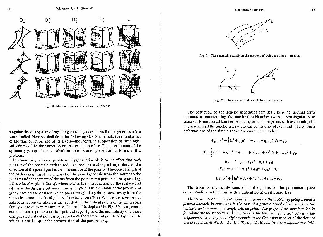
V.I. Amol’d, A.B. Givental’ Symplectic Geometry 111
Fig. 50. Metamorphoses of caustics, the D series
singularities of a system of rays tangent to a geodesic pencil on a generic surface were studied. Here we shall describe, following O.P. Shcherbak, the singularities of the time function and of its levels-the fronts, in supposition of the single- valuedness of the time function on the obstacle surface. The discriminant of the symmetry group of the icosahedron appears among the normal forms in this problem.
In connection with our problem Huygens’ principle is to the effect that each point x of the obstacle surface radiates into space along all rays close to the direction of the pencil geodesic on the surface at the point x. The optical length of the path consisting of the segment of the pencil geodesic from the source to the point x and the segment of the ray from the point x to a point q of the space (Fig. 5 1) is F(x, q) = 4(x) + G(x, q), where 4(x) is the time function on the surface and G(x, q) is the distance between x and q in space. The extremals of the problem of going around the obstacle which pass through the point q break away from the obstacle surface at critical points of the function F(., q). What is decisive for our subsequent considerations is the fact that all the critical points of the generating family F are of even multiplicity. The proof is depicted in Fig. 52: to a generic extremal corresponds a critical point of type A,, and the multiplicity of a more complicated critical point is equal to twice the number of points of type A, into which it breaks up under perturbation of the parameter q.
Fig. 51. The generating family in the problem of going around an obstacle
Fig. 52. The even multiplicity of the critical points
The reduction of the generic generating families F(x, q) to normal form amounts to enumerating the maximal subfamilies (with a nonsingular base space) of R-miniversal families belonging to function germs with even multiplic- ity, in which all the functions have critical points only of even multiplicity. Such deformations of the simple germs are enumerated below.
A;,: y2+[(uk+qIuk-z+. . +q,-,)2du+q,;
D;,: j(uk-l+qluk-2+. . . +qk-2U+X)‘du+qk-1x+qk; 0
Ek: x3+y4+qIy2+q2y+q3;
E’,: x3+y5+q,y3+q,y2+q,y+q,;
E’,‘: x3+j(u2+qIx+q2)2du+q3x+q4; 0
The front of the family consists of the points in the parameter space corresponding to functions with a critical point on the zero level.
Theorem. Thefunctions of a generatingfamily in the problem of going around a generic obstacle in space and in the case of a generic pencil of geodesics on the obstacle surface have only simple critical points. The graph of the time function in four-dimensional space-time (the big front in the terminology of sect. 3.4) is in the neighbourhood of any point difleomorphic to the Cartesian product of the front of one of the families A;, AL, A;, L14, D& D& EL, E18, E’{ by a nonsingular manifold.

112 V.I. Amol’d, A.B. Givental’ Symplectic Geometry 113
Examples. 1) To the family A; correspond the nonsingular points of the front.
2) The self-intersection line of the swallowtail-the latter is the caustic of an R +-versa1 deformation of the germ &-corresponds to the functions with two critical points of type A,. This is how one obtains the family Ai of the preceding list. Its front q2 - _ +q:” is diffeomorphic to the discriminant of the symmetry group H, of the regular pentagon.
3) In Fig. 53a is shown the metamorphosis of a front in the neighbourhood of an inflection point of an obstacle on the plane. The graph of the time function (Fig. 53b) is diffeomorphic to the discriminant of the symmetry group H, of the icosahedron’3. The discriminant of H, is the front of the family L)& It is also diffeomorphic to the front in the neighbourhood of the points on an obstacle surface in space at which the pencil geodesic has an asymptotic direction.
( .gyh.@ Fig. 53. Going around an obstacle in R2 and the icosahedron discriminant
4) After breaking away from the obstacle surface in a nonasymptotic direc- tion, the rays may become focused far away from it, forming a caustic. The metamorphoses of the front in the neighbourhood of a nonsingular point, a point on a cusp ridge, or a swallowtail vertex of such a caustic are described by the families Dk (x3 - y3 + qly+ q2), Ek and E’,. These families can be obtained from the R-versa1 families of the germs A,, A,, A4 by addition of the cube of a new variable. This operation turns all critical points of the functions of the original family into ones of even multiplicity, but does not change its front.
5) In the classification of regular polytopes (see [ 14]), just after the pentagon and the icosahedron comes a body with 120 vertices in four-dimensional space. It can be described as follows. The Lie group SU, of quaternions of unit length contains the binary group of the icosahedron (see sect. 2.4). Its 120 elements are just the vertices of our polytope in the space of quaternions. The discriminant of the symmetry group H, of this polytope is diffeomorphic to the front of the
I3 A different description: the union of the tangents to the curve (t, t3, t’) in R3.
family Ei. In the problem of going around an obstacle this front is encountered as the graph of the time function in the neighbourhood of a point of intersection of an asymptotic ray with a cusp ridge of the caustic far away from the obstacle surfacei4.
If we now turn to the classification of the irreducible Coxeter groups-finite groups generated by reflections but not necessarily preserving an integral lattice (see [14]), then we will discover that among the wave fronts in the various problems of geometrical optics, we have encountered the discriminants of all such groups except for the symmetry groups of the regular n-gons with n 2 6.
Chapter 6
Lagrangian and Legendre Cobordisms
Cobordism theory studies the properties of a smooth manifold which do not change when it is replaced by another manifold of the same dimension which together with the first forms the boundary of a manifold of dimension one greater (Fig. 54). In this chapter the manifolds and the sheets bounded by them will be Lagrangian or Legendre submanifolds. The corresponding cobordism theories reflect, for example, the global properties of wave fronts which are preserved under metamorphoses.‘5 \ G :
Fig. 54. Cobordism
0 1. The Maslov Index
A Lagrangian submanifold of a phase space describes the phase of a short- wave oscillation. The Maslov index associates integers to the curves on the
I4 Such a ray breaks away from the obstacle at a parabolic point. I s Beginning with 3 2, we are compelled to abandon all concern for the inexperienced reader. By
way of compensation. 5 1 includes a completely elementary exposition of the theory of cobordisms of wave fronts on the plane.
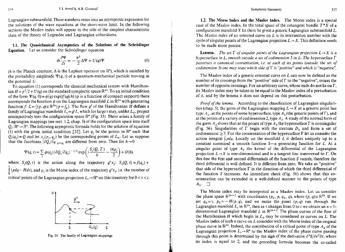
113 V.I. Amol’d, A.B. Givental’ Symplectic Geometry 115
Lagrangian submanifold. These numbers enter into an asymptotic expression for the solutions of the wave equations at the short-wave limit. In the following sections the Maslov index will appear in the role of the simplest characteristic class of the theory of Legendre and Lagrangian cobordisms.
1.1. The Quasiclassical Asymptotics of the Solutions of the Schriidinger Equation. Let us consider the Schrodinger equation
ihg= -g*Y+U(q)Y! (1)
(h is the Planck constant, A is the Laplace operator on R”), which is satisfied by the probability amplitude Y(q, t) of a quantum-mechanical particle moving in the potential U.
To equation (1) corresponds the classical mechanical system with Hamilton- ian H =p2/2 + U(q) on the standard symplectic space R2”. To an initial condition of the form Y (q, 0) = 4(q) exp(if(q)/h) (4 is a function of compact support) there corresponds the function C#I on the Lagrangian manifold L in lR2” with generating function f: L = ((p, q) E lR*” 1 p =f,}. The flow g’ of the Hamiltonian H defines a family of Lagrangian manifolds L, = g’L, which for large t may, unlike L,, project noninjectively into the configuration space R” (Fig. 55). There arises a family of Lagrangian mappings (see sect. 1.2, chap, 5) of the configuration space into itself Q,: R”+ KY. The following asymptotic formula holds for the solution of equation (1) with the given initial condition [.52]. Let qj be the points in R” such that Q,(qj)=Q and let xj(pj, qj) be the corresponding points of L,. Let us suppose that the Jacobians /aQ,/aq lqE4, are different from zero. Then for h-t0
y(q, t) = 1 +(qj) IdQtldqj I- 1'2 exp i sj(Q, T)
h - y +0(h), j >
where S,(Q, t) is the action along the trajectory g’Xj: Sj(Q, t) =f(qj)+
[(Pdq-Hd )T d j’ r an p IS the Morse index of the trajectory g’xj, i.e. the number of
critical points of the Lagrangian projection L, + R” on this traectory for 0 -C r ct.
pt
I !L /q--F )
e Qde, e
Fig. 55. The family of Lagrangian mappings
1.2. The Morse Index and the Maslov Index. The Morse index is a special case of the Maslov index. In the total space of the cotangent bundle T*X of a configuration manifold X let there be given a generic Lagrangian submanifold L. The Masloc index of an oriented curve on L is its intersection number with the cycle of singular points of the Lagrangian projection L-+X. This definition needs to be made more precise.
Lemma. The set I- of singular points of the Lagrangian projection L-+X is a hypersurface in L, smooth outside a set of codimension 3 in L. The hypersurface r possesses a canonical coorientation, i.e. at each of its points (outside the set of codimension 3) one may state which side of r is “positive” and which is “negative”.
The Maslov index of a generic oriented curve on L can now be defined as the number of its crossings from the “positive” side of r to the “negative”, minus the number of opposite crossings. For an arbitrary curve, whose ends do not lie on r, its Maslov index may be taken to be equal to the Maslov index of a perturbation of it, and by the lemma it does not depend on this perturbation.
Proof of the lemma. According to the classification of Lagrangian singulari- ties (chap. 5), the germ of the Lagrangian mapping L-+X at a generic point has type A r, at the points of some hypersurface, type A, (the generic points of r), and at the points of a variety of codimension 2, type A,. A study of the normal form of the germ A, shows that at the points of type A, the hypersurface JY is nonsingular (Fig. 56). Singularities of r begin with the stratum D, and form a set of codimension 2 3. For the coorientation of the hypersurface r let us consider the action integral fpdq. Locally on the manifold L it defines uniquely up to a constant summand a smooth function S-a generating function for L. At a singular point of type A, the kernel of the differential of the Lagrangian projection L+X is one-dimensional and is a tangent line transversal to r. On this line the first and second differentials of the function S vanish; therefore the third differential is well defined. It is different from zero. We take as “positive” that side of the hypersurface r in the direction of which the third differential of the function S increases. An immediate check (Fig. 56) shows that this CO-
orientation can be extended in a well-defined manner to the points of type A,. 0
The Morse index may be interpreted as a Maslov index. Let us consider the phase space lR2n+2 with coordinates (p,,, p, q,,, q), where (p, q) E R2”. If we set qO=t, pO= - H(p, q), and we make the point (p; q) run through the Lagrangian manifold L, in R2n, then as T changes from 0 to t we obtain an n + l- dimensional Lagrangian manifold L in [w 2”+2. The phase curves of the flow of the Hamiltonian H which begin in L, may be considered as curves on L. The Maslov index of such a curve on L coincides’with the Morse index of the original phase curve in R2”. Indeed, the contribution of a critical point of type A, of the Lagrangian projection L,+R” to the Maslov index of the phase curve passing through this point is determined by the sign of the derivative ~3S/~u2~7, where its index is equal to 2, and the preceding formula becomes the so-called

116 V.I. Amol’d, A.B. Givental Symplectic Geometry 117
“quantization condition” (see the article by A.A. Kirillov in this volume)
Fig. 56. The coorientation of the cycle I’
S = l (pdq - Hdt) is a generating function for L, and u is a vector from the kernel of the differential of the projection L 4 lRZ”+Z+iRnc ’ at the critical point under consideration. This sign is always negative in view of the convexity of the function H = p2/2 + U(q) with respect to the momenta. Therefore each critical point lying on the phase curve gives a contribution of + 1 both to its Maslov index and to the Morse index.
1.3. The Maslov Index of Closed Curves. The intersection number of a closed curve on a Lagrangian manifold L c T*X with the cooriented hypersurface I of singular points of the projection L +X does not change upon replacement of the curve by a homologous one. Therefore r defines a Maslou class in the cohomology group H’(L, Z).
The Maslov indices of closed curves enter into the asymptotic formulas for the solutions of stationary problems (characteristic oscillations) [52]. Let us suppose that on the level manifold H = E of the Hamiltonian H = p2/2 + U(q) there lies a Lagrangian submanifold L. If a sequence of numbers pN-’ cc satisfies the conditions
G$pdy--indy(mod4) Y
for all closed contours y on L (for the existence of the sequence pN the existence of at least one such number p#O is sufficient), then the equation AY/2 = I.‘( U(q) - E)Y has a series of eigenvalues & with the asymptotic behaviour ~N=PN+o(Pil).
In the one-dimensional case the Lagrangian manifold is an embedded circle, its index is equal to 2, and the preceding formula becomes the so-called
For example, in the case H =p2/2 + q2/2 with the given Planck constant h= l/,u we obtain the exact values for the characteristic energy levels E, = h( N + i), N = 0, 1, . . . of the quantum harmonic oscillator.
The Maslov class of Lagrangian submanifolds of the standard symplectic space R2” is the inverse image of a universal class of the Lagrangian Grassmann manifold A, under the Gauss mapping. The Gauss mapping G: L + A, associates to a point of the Lagrangian submanifold the tangent Lagrangian space at that point, translated to 0. The cohomology group H’(A,, Z) is isomorphic to Z.
Theorem. The generator of the group H’(A,, Z) goes over into the Maslov class under the homomorphism G*: H’(A,, if)-, H ‘(L, Z).
Corollary. The Masiov class of a Lagrangian submanifold in R2” does not depend on the Lagrangian projection R’“+ &I”.
Below we shall cite two descriptions of the generators in the group H’V,, 0
1.4. The Lagrangian Grassmann Manifold and the Universal Maslov Class. The Lagrangian Grassmann manifold A,, is the manifold of all Lagrangian
linear subspaces of the 2n-dimensional symplectic space. The manifold of all oriented Lagrangian subspaces in R”’ is called the oriented Lagrangian Grassmann manifold and is denoted by A,‘. Obviously 12: is a double covering of A,,.
Examples. 1) A, = RP’ z A: = S’. 2) The manifold A, is isomorphic to the quadric x2 + y2 + a2 = u2 + v2 in RP4
as a projective algebraic manifold (see sect. 1.3, chap. 1). The manifold A: is diffeomorphic to S2 x S’. The covering A: +A2 is the factorization of S2 x S’ by the antipodal involution (x, y)~( -x, - y) (in [37] A2 is found incorrectly).
3) dim A,,= n(n+ 1)/2: a generic Lagrangian subspace in R2” is given by a generating quadratic form in n variables.
Theorem. The Grassmann manifolds of Lagrangian subspaces in C” are
homogeneous spaces: A, =U,/O,, A,’ =U,/SO,, where U,, O,, SO, are the unitary, orthogonal and special orthogonal groups respectively.
Indeed, an orthonormal basis of a Lagrangian subspace in @” is a unitary basis in @” and conversely, the real linear span of a unitary frame in @” is a Lagrangian subspace. Unitary bases which generate the same Lagrangian subspace can be obtained from each other by an orthogonal. transformation of this subspace. I-J
Corollary. x1 (A,) = H 1 (A,, Z) z H r (A,, h) z Z.

118 V.I. Arnol’d, A.B. Givental’
Let us consider the mapping de?: U,+C ‘, which associates to a unitary matrix the square ofits determinant. The mapping det’ well-defines a fibration of the Lagrangian Grassmann manifold An over the circle S’ = {eib} of complex numbers of modulus 1. The fibre SUJSO, of this fibration is simply connected, and therefore the differential l-form a=( 1/2x)(det*)*@ on A, represents a generator of the one-dimensional cohomology group H’(A,, Z). We shall call this generator the universal Maslov class.
Example. det2: A, +S’ is a diffeomorphism, and a=dO/z, where B is the angular coordinate of the line 1 E/\~ on the plane R*.
Let us define an inclusion i: A,,- 1 4 A, in the following manner. Let H be a hyperplane in R2”. The projection H+ H/H’ into the 2n - 2-dimensional symplectic space of characteristics of the hyperplane H establishes a one-to-one correspondence between the n- l-dimensional Lagrangian subspaces in H/H’ and the n-dimensional Lagrangian subspaces lying in H.
Lemma. The inclusion j induces an isomorphism of the fundamental groups.
Indeed, the sequence ofinclusions A1 4 A2 4 . . . 4 A,, maps the circle A1 into a circle S over which the integral of the l-form c( on A, is equal to 1, i.e. the inclusion A1 4 A, induces an isomorphism nl(A1)+n,(A,). 0
Let us now present the cycle which is dual to the generator of the group H ‘(A”, Z) = Z. Let us fix a Lagrangian subspace L c R*” and let us denote by C the hypersurface in A, formed by the Lagrangian subspaces in IX*” which are not transversal to L. The Lagrangian spaces in R*” which intersect L along subspaces of dimension 2 or more form a set Y of codimension 3 in A,, (and 2 in C). At points AEX\Z’ the hypersurface C is smooth. Let us coorient Z by choosing as a vector of the positive normal at the point 3, the velocity vector of the curve e”i, (it is transversal to C).
Theorem. The intersection number of a l-cycle in A,, with the cooriented cycle C is equal to the value of the universal Maslov class on this l-cycle.
Indeed, the intersection number of the generator S of the group H, (A,,.Z) with the cycle C is equal to 1. 0
The cycle r of singularities of the projection of a Lagrangian submanifold in [w*” along the Lagrangian subspace L is the inverse image of the cycle C under the Gauss map. From this the theorem of sect. 1.3 follows. IJ
Remark. The Maslov index has found application in the theory of represen- tations [49]. In this context a series of Maslov indices is used-symplectic invariants of chains of k Lagrangian subspaces in R*“. The simplest of them is the triple index r(i., , i,,, &), equal to the signature of the quadratic form Q(x1@x2@x3)=~(x1, x2)+o(x2,xj)+o(xg, x1) on the direct sum of the Lagrangian subspaces 3,, @ ;1, @A,, where w is the symplectic form on R2”. It has thecocycle property: r(ll,, i,,, &)-7(&, i.,, &)+7(i1, i,,, &)-7(&, &, &)=O.
Symplectic Geometry 119
With the aid of the Maslov index of a quadruple of subspaces r(i., , i.,, &) + 7(3.,, &, &) one may define on a Lagrangian submanifold in the total space of the cotangent bundle of an arbitrary manifold a Tech cocycle corresponding to the Maslov class of sect. 1.3 (see [37]).
1.5. Cobordisms of Wave Fronts on the Plane. The simplest example of a Legendre cobordism is the relation between the traces of a wave front spreading in a three-dimensional medium on its boundary at the various moments of time. These traces are not necessarily homeomorphic, but their being cobordant imposes a restriction on the types of the singularities (see Corollary 1 below).
Two compact wave fronts F,, F, on the plane are called cobordant, if in the direct product of the plane with the interval 0 <t I 1 there exists a compact front K transversal to the planes t = 0 and t = 1 whose intersection with the first of these is F, and with the second, F, (Fig. 57). The front K is called a cobordism. We distinguish the cases of oriented and nonoriented, armed (cooriented) or un- armed fronts and cobordisms. An armament of a cobordism K induces an armament of the boundary dK = F0 u F,, which must coincide with the own armament of the fronts F07 F, (i.e. fronts which coincide but which are spreading to different sides are considered different and may be incobordant). The same also relates to orientations. The addition of fronts is defined as their disjoint union. This operation provides the set of classes of cobordant fronts with the structure of a commutative semigroup. In the cases being considered it turns out to be a group. The class of the empty front serves as the zero element.
Fig. 57. Cobordism bf fronts in Wz
Theorem ([S]). The group of cobordism classes of armed orientedfronts on the plane is free cyclic (the generator is the class of the “bow”, Fig. 58a), of armed nonoriented ones is trivial, and of unarmed ones is finite: 7, @ Z, for oriented and Z, for nonoriented fronts (as generators one may take the classes of the “drops”, Fig. 58b, which differ in the orientation in the oriented case).
What serves as the unique invariant of the cobordism class of an armed oriented front on the plane is its index-the number of cusp points (or the number of inflection points) with signs taken into account, Fig. 58~. The index of a compact front in R2 is even.

120 V.I. Amol’d, A.B. Givental’
a
btlb -2 2
C e 8
r' i'
Fig. 58. a) the bow b) the drop c) the Maslov index of an armed front
Corollary 1. The algebraic number of cusp (inflection) points of the compact trace on the plane of an oriented wave front spreading in space is even and does not change with time.
The index of a front is connected with the Maslov index in the following way. An armed front in R* defines the conical Lagrangian surface L in T*R* of covectors equal to zero on a contact element tangent to the front and positive on the arming normal. For a generic front L is smoothly immersed in T*R*. The scalar praduct on R* defines an immersion of the front into L (to a point of the front corresponds the covector equal to 1 on the unit vector of the arming normal). The index of an oriented front in lR* is equal to the Maslov index of the constructed curve on L.
The computation of the cobordism groups described in the theorem is based on the information on metamorphoses of wave fronts from sect. 3.4 of chap. 5. Thus, the nonoriented cobordance to zero of the armed bow follows from the series of restructurings of Fig. 59, using the local metamorphoses A, and A, of Fig. 48.
Fig. 59. The unoriented bow is cobordant to zero
Symplectic Geometry 121
A cobordism K of fronts defines the immersed Legendre manifold of its contact elements in the manifold of all contact elements of the product of the plane with the interval.
Corollary 2. The Klein bottle admits a Legendre immersion into R5.
This immersion is induced by the metamorphoses of Fig. 59 together with the reverse series: the fronts being bifurcated in this drawing have a nonvertical tangent everywhere and their union glues the “bow” by means of a Mdbius strip. 0
Theorem ([S], compare sect. 2.4, chap. 4). The compact connected two- dimensional manifolds with an even Euler characteristic admit a Legendre immer- sion into the contact space R5, but those with an odd Euler characteristic do not even admit a Lagrangian immersion into R4.
6 2. Cobordisms
In [S] about a score of different Lagrangian and Legendre cobordism theories are defined and the corresponding groups of classes of cobordant curves are computed. Here we shall consider in the main the cobordisms of exact Lagrangian immersions-the theory in which the most complete results have been obtained.
2.1. The Lagrangian and the Legendre Boundary. In the total space of the cotangent bundle of a manifold with boundary let there be given an immersed Lagrangian submanifold L CG T*M, transversal to the boundary a( T*M). Under the mapping a( T*M)+ T*(dM) (to a covector at a point of the boundary is associated its restriction to the boundary) the intersection Lna( T*M) projects to an immersed Lagrangian submanifold 2L of the total space of the cotangent bundle of the boundary. 8L is called the Lagrangian boundary of the manifold L.
The Legendre boundary 8L of a Legendre manifold L 4 J ‘M immersed in the space of l-jets of functions on a manifold with boundary and transversal to the boundary a(J’M) is defined analogously with the aid of the projection 8(J’M)+J’(ZM) (to the l-jet of a function at a point of the boundary is associated the l-jet of the restriction of the function to the boundary). In a similar way one can define the boundary of a Legendre submanifold of the space of (cooriented) contact elements on a manifold with boundary.
A Lagrangian cobordism of two compact Lagrangian immersed sub- manifolds LO, L, CG T *M is an immersed Lagrangian submanifold of the space T *(M x [0, l]), the cotangent bundle of the cylinder over M, whose Lagrangian boundary is the difference of L, x 1 and LO x 0 (for oriented cobordisms changing the orientation of a manifold changes its sign). The manifolds L,, L,

122 V.I. Amol’d, A.B. Givental’
are called Lagrangianly (orientedly) cobordant, if there exists a Lagrangian (oriented) cobordism between them.
Legendre cobordisms are defined analogously. In this case in place of cobor- dism of Legendre manifolds one may speak directly of cobordism of fronts. The theory of cobordisms of Legendre immersions in the space of 1 -jets of functions is equivalent to the theory of cobordisms of exact Lagrangian immersions: under the projection J ‘M + T*M the Legendre immersed submanifolds go over into Lagrangian immersed submanifolds on which the action l-form is exact, and conversely (see sect. 2.3, chap. 4).
2.2. The Ring of Cobordism Classes. Lagrangian (Legendre) immersions of manifolds L,, L, of the same dimension into a symplectic (contact) manifold give an immersion of their disjoint union into this manifold, called the sum of the original immersions.
Lemma ([5]). The classes of Lagrangianly (Legendrianly) cobordant immer- sions into T*M (J’M, PT*M or ST*M)f orm an abelian group with respect to the summation operation.
In the simplest and most important case M = IR” let us define the product of two (exact) Lagrangian immersions L, 4 T*R”, L, 4 T*Rm as the (exact) Lagrangian immersion of the direct product L, x L, in T*R”+“‘= T*R” x T*W’ The corresponding cobordism classes form a skew-commutative graded ring with respect to the operations introduced.
Theorem ([7], [12], [19]). 1) The graded ring 9X, = @‘%z[L, ofnonoriented
Legendre cobordism classes in the spaces of 1 -jets offunctiols on iRk is isomorphic to the graded ring Z,[x,, x9, xI1,. . .] of polynomials with coeficients in Z, in generators xk of odd degrees k # 2’- 1.
2) The graded ring II,= @[Lk oriented Legendre cobordism classes in the
spaces of l-jets offunctions on ‘Rk is isomorphic (after tensor multiplication with Q) to the exterior algebra over Q with generators of degrees 1,5,9, . . . , 4n + 1, . .
We are far from being able to prove this theorem, but we shall cite the fundamental results on the way to its proof.
2.3. Vector Bundles with a Trivial Complexification. Every k-dimensional vector bundle with a finite CW base space X can be induced from a universal classifying bundle rk. As the latter one may take the tautological bundle over the Grassmann manifold G,, k of all k-dimensional subspaces in a space RN of growing dimension N (serving as the fibre of the tautological bundle over a point is the k-dimensional subspace which answers to that point). The induction of a bundle over X under a continuous mapping X + G,., establishes a one-to-one correspondence between the equivalence classes of k-dimensional vector bundles
Symplectic Geometry 123
with the base space X and the homotopy classes of mappings of X into the classifying space G,. k. In the category of oriented vector bundles the role of the classifying spaces is played by the Grassmann manifolds Gz.k of oriented k- dimensional subspaces.
Let the complexification of a real k-dimensional vector bundle over X be trivial and let a trivialization be fixed.
An example: the complexification of a tangent space L to a Lagrangian manifold immersed in the realification Rzk of the Hermitian space Ck is canonically isomorphic to @’ = L 0 iL.
If we associate to a point in X the subspace of Ck with which the fibre over it is identified under the trivialization, we get a mapping of X into the Grassmann manifold of k-dimensional real subspaces L of Ck for which L n iL=O. This Grassmann manifold is homotopy equivalent to the Lagrangian Grassmann manifold A,.
Theorem ([27]). The tautological bundle i., (1.: ) over the (oriented) Lagran- gian Grassmann manifold A, (A:) is classifying in the category of k-dimensional (oriented) vector bundles with a trivialized complexification.
2.4. Cobordisms of Smooth Manifolds. In this classical theory two closed manifolds (immersed nowhere) are called cobordant, if their difference is the boundary of some compact manifold with boundary. In the computation of the corresponding cobordism groups the key role is played by the ‘following construction. By the Thorn space Ti of a vector bundle i’ with a compact base space is meant the one-point compactification of the total space of this bundle (Fig. 60). For an induction of a bundle 5 from a bundle v under a mapping of the base spaces X-r Y there is a corresponding mapping T<-+ Tn of the Thorn spaces, which takes the distinguished point (co) over into the distinguished point. Let the compact n-dimensional manifold M be embedded in a sphere of large dimension n + k. Collapsing the complement of a tubular neighbourhood of M in
Fig. 60. The Thorn space

124 V.I. Arnol’d, A.B. Givental
S n+ k to a point gives a mapping S n+k+ TV of the sphere to the Thorn space of the normal bundle of the manifold M. The induction of the normal bundle from the classifying bundle tk furnishes a mapping TV+ T<, of Thorn spaces, which in composition with the first defines a mapping Sn+k+T<k. An analogous construction, applied to a cobordism of manifolds which is embedded in S n+k x [0, 11, shows that for a cobordism class there is a corresponding homotopy class of mappings S”+k-+T5k, i.e. an element of the homotopy
group %+,( % co). Conversely, the inverse image of the zero section Gs,k 4 Ttk under a mapping of the sphere Sn*k+ T& transversal to it is a smooth n-dimensional submanifold in Snfk, and the inverse image of the zero section under a homotopy S”+k x [0, l] + Tt, transversal to it is a cobordism of such manifolds.
Theorem ([69]). The group 9I, (Q,) of(oriented) cobordism classes ofclosed n- dimensional manifolds is isomorphic to the stable homotopy group lim rr, +k( Ttk) of
k-m
the Thorn spaces of the classifying (oriented) vector bundles.
Here the symbol lim denotes the following. A mapping Sn+k + Tt, can be suspended to a mapping S ni-ki- ’ + T(t, @ 1) of the sphere to the Thorn space of the sum of the bundle tk with the one-dimensional trivial bundle. This sum can be induced from tk + 1, which gives a mapping Sn+k+ ’ + Ttk+ 1. It is over the so arising sequence of homomorphisms n, + k( Ttk) + n, + k + r ( Tck + 1 ) that the limit is taken.
This theorem reduces the computation of cobordism groups to a purely homotopic problem, which one can succeed in solving to a significant degree.
Theorem ([69]). 1) The ring 3, = @%, is isomorphic to the ring Z, [y2, y,,
Y5,. . .] of polynomials over Z, in generators y, of degrees n # 2’- 1. 2) The ring R, = @Q,, is isomorphic modulo torsion to the ring of polynomials
over Z with generators of degrees 4k, k= 1, 2, . . . .
2.5. The Legendre Cobordism Groups as Homotopy Groups. Let us associate to a Legendre immersion of a manifold L in J ‘R” a trivialization of the complexified tangent bundle TcL, as explained in the example of sect. 2.3.
Theorem ([36], [46]). This mapping is a one-to-one correspondence between the set of homotopy classes of Legendre immersions L 4 J’R” and the set of homotopy classes of trivializations of the bundle T ‘L.
From this, just as in the theory of cobordisms of smooth manifolds, one can deduce
Theorem (Ya.M. Ehliashberg, see [19]). The groups of Legendre cobordism classes are isomorphic to the stable homotopy groups of the Thorn spaces of the
Symplectic Geometry 125
tautological bundles over the Lagrangian Grassmann manifolds:
‘%L, = lim x,+~( TAk), 11, = lim x”+~( TA,,?). k-w k-x
The passage to the limit is in correspondence with the sequence of inclusions of Lagrangian Grassmann manifolds described in sect. 1.4.
An analogous expression for the cobordism groups through homotopy groups (of more unwieldy spaces, it is true) holds also for the other Lagrangian and Legendre cobordism theories’ 6, but these homotopy groups have at present not been computed.
The computation of the stable homotopy groups of the spaces Ti,, leads to the following refinement of the theorem of sect. 2.2.
Theorem ([ 123). The mapping 8: 9I [L, + 912, which associates to the cobordism class of an immersed Legendre manifold the nonoriented cobordism class of this manifold is an inclusion of graded rings and ‘!R2, = 6(%~,.@Zz[yz, . . . , yzk, . . .].
Corollary. The nonoriented Legendre cobordism class of a Legendre immersion L 4 J ‘R” depends only on the manifold L.
2.6. The Lagrangian Cobordism Groups. These groups are as a rule too large to be readily visible. Only the Lagrangian cobordism groups of curves on surfaces have been computed [5]. The point is that the action integral over a closed curve on a Lagrangian cobordism-manifold depends only on the homology class of the curve on it. If the action integrals over a basis of l-cycles on a Lagrangianly immersed closed manifold L are rationally independent, then the space H,(L, Q) together with the linear real-valued function on it defined by the cohomology class of the action form is an invariant of the Lagrangian cobordism class of the manifold L.
A Lagrangian immersion L 4 T*R”, along’with the Gauss mapping L-A,, gives a mapping L+K(R, 1) into the Eilenberg-MacLane space of the additive group of real numbers (rc,(K(R, l))= R, r&(K@, I))=0 for k# l), defined by the homomorphism of the fundamental groups rte(L)+HH(L, Q)-+R.” Let T, be the Thorn space of the bundle over K(R, 1) x A,’ induced from the tautological bundle by the projection onto the second factor.
Theorem.” The group of oriented Lagrangian cobordism classes in T*R” is
lim %+k( Tk). k-m
I6 See Ya.M. Ehliashberg’s article in [19]. ” The first of these two maps is the Hurewicz homomorphism, and the second is the cohomology
class of the restriction to L of the Liouville l-form pdq on the cotangent bundle T*R”, which on L is closed because L is Lagrangian. The homomorphism H, (L, Q)- R may be thought of as being given by integration of this I-form along the I-cycles. (Note added in translation).
ts See Ya.M. Ehliashberg’s article in [19].

126 V.I. Amol’d. A.B. Givental
For n = 1 this group is R @ Z-the only (and independent) invariants of the Lagrangian cobordism class of a closed curve on the symplectic plane are its Maslov index and the area of the region bounded by the curve [S].
4 3. Characteristic Numbers
Here we shall describe discrete invariants of the Lagrangian (Legendre) cobordism class. They arise from cohomology classes of the Lagrangian Grassmann manifolds, but they receive a geometric interpretation in the calculation of Lagrangian and Legendre singularities. This circumstance sheds light on the algebraic nature of the classification of critical points of functions.
3.1. Characteristic Classes of Vector Bundles. When a vector bundle is induced by a mapping of the base space into a classifying space a cohomology class of the classifying space determines a cohomology class of the base space, called a characteristic class of the bundle. The original cohomology class of the classifying space is called the universal characteristic class. If two bundles of the same dimension with a common base space have different characteristic classes obtained from one universal class, then these bundles are inequivalent.
The sequences of homomorphisms of the cohomology groups corresponding to the sequences of inclusions
define the stable cohomology groups of the corresponding Grassmann mani- folds.
Theorem ([56], [27]). The graded stable cohomology rings of the Grassman‘n manifolds are as follows:
1) H*(G+, Q) = Q[pl, . . , pk, . ] is the ring of polynomials with rational coefficients in the integral Pontryagin classes pk of degree 4k;
2) H*(G, Z,) = Z,[w,, . . . , wk, . . . ] is the ring of polynomials over thefield Z, in the Stiefel-Whitney classes wk of degree k;
3) H*(A+, Q) is an exterior algebra over Q with integral generators of degrees 4k+l,k=0,1,2 ,...;
4) H*(A, Z’,) is the exterior algebra over Z, in the Stiefel- Whitney classes.
Remarks. 1) The kernel of the epimorphism H*(G, Z,)-+ H*(A, Z,) defined by the inclusions A,, 4 GZn.” 4 G,., is the ideal generated by the squares [28]. We note that the dimension of the space Hk(A, 77,) over the field Z, is equal to the number of partitions of k into a sum of different natural-number summands.
Symplectic Geometry 127
2) Every nonzero element of the cohomology rings enumerated in the theorem defines a nontrivial universal characteristic class which distinguishes the stable Tquivalence classes of (oriented) vector bundles and of (oriented) vector bundles with a trivialized complexification respectively.
3.2. The Characteristic Numbers of Cobordism Classes
Lemma. The value of an n-dimensional stable characteristic class of the tangent bundle of an n-dimensional closed manifold on its fundamental cycle depends only on the cobordism class of this manifold.
Indeed, the restriction of the tangent bundle of a manifold to its boundary is isomorphic to the sum of the one-dimensional trivial bundle and the tangent bundle of the boundary, i.e. it is stably equivalent to the latter. The value of a stable characteristic class of the tangent bundle of the manifold on the fundamental cycle of the boundary is equal to zero, since this cycle is homologous to zero. 0
Thus, each stable universal n-dimensional characteristic class defines a characteristic number of a closed n-dimensional manifold-an invariant of the cobordism class of this manifold. Analogously, characteristic numbers of a Lagrangian (Legendre) immersion into T*R” (.I’ R”) are defined by the n- dimensional characteristic classes of a trivialization of the complexified tangent bundle of the immersed manifold and they are invariants of the Lagrangian (Legendre) cobordism class. Obviously, the characteristic number of a sum of cobordism classes is equal to the sum of the characteristic numbers of the summands.
Theorem ([12]). 1) The group homomorphism CJziL, + H,(A, Z,) given by the Stiefel- Whitney characteristic numbers is a monomorphism.
2) The analogous homomorphism IL,,-+ H,(A’, Z) is a monomorphism and becomes an isomorphism after tensoring with Q.
Corollary. The nonoriented Legendre cobordism class of a Legendre immersion in J 1 [w” is determined by the Stiefel- Whitney numbers of the immersed manifold,
Remarks. 1) An analogous theorem is true for the cobordism theory of closed manifolds.
2) The number of partitions of a natural number k into a sum of odd summands-the dimension of the subspace H, of the graded ring @H, of polynomials over Z, in generators of odd degree-is equal to the number of partitions of k into distinct summands (we split each even summand into a sum of 2’ identical odd ones. . . ).
3) Between the Stiefel-Whitney numbers of Legendre immersions there are relations. For example, the Maslov index of a closed Legendre curve in J ‘[w is even, i.e. the characteristic number wI = 0.

128 V.I. Arnol’d, A.B. Givental’
4) The multiplication of characteristic classes together with the multiplication of the objects dual to them-the cobordism classes-gives a Hopf algebra structure on H = 1, @ Q: the comultiplication H + H @ H is an algebra homomorphism.
5) The corollary has no analogue in the oriented case: the Pontryagin classes of the tangent bundle of a manifold which admits a Lagrangian immersion in T*R” are zero.
3.3. Complexes of Singularities. Let us partition the space of germs of smooth functions of one variable at a critical point 0 with critical value zero (more precisely-the space ofjets of such functions of sufficiently high order) into nonsingular strata-the R-equivalence classes (see 3 2, chap. 5) of A:, A,, A:, A . . . and the class containing the zero function. We shall call a stratum of f$;te codimension coorientable if its normal bundle possesses an orientation invariant with respect to the action of the group of germs of diffeomorphisms on the space of germs of functions. Those which prove to be noncoorientable are the strata A&- 1 and only they. For example, the transversal to the stratum A: at the point x4 may be taken of the form x4 + i., x3 + i.,x’; the substitution x w -x changes the orientation of the transversal. Let us define a complex w whose group of k-chains consists of the formal integral linear combinations of the cooriented strata of codimension k. Changing the orientation changes the sign of the stratum. The coboundary operator 6 is defined using the adjacencies of strata like the usual operator of taking the boundary of chains. We remark that a noncoorientable stratum enters into the boundary of a coorientable one with coefficient zero, and therefore the operator 6 is well-defined and J2 = 0. The complex v, which does not take into account the coorientation of the strata, consists of the formal sums with coefficients in the field Z, of all strata and is provided with an operator of taking the boundary of a stratum modulo 2.
We have used the classification of critical points of functions on the line only as an illustration. In reality we need universal complexes o and v defined analogously with respect to a discrete stratification of the spaces of germs of functions of an arbitrary number of variables into nonsingular strata which are invariant with respect to stable R-equivalence of germs.
Let there be given a generic Lagrangian immersion L 4 T*M”. The Lagrang- ian projection into M” defines a stratification of the manifold L according to the types of the singularities of the Lagrangian mapping L + M” in correspondence with the stratification of the space of germs of functions.
Theorem (V.A. Vasil’ev [71]). To each (cooriented) cycle of the universal complex v (CO) there corresponds a (cooriented) cycle of the closed (oriented) manifold L with coefficients in Z, (Z). A homology class of the complex v (CO) defines a cohomology class of the manifold L with coeficients in Z, (Q-the intersection number of cycles on L with the corresponding (cooriented) cycle of singularities.
Symplectic Geometry 129
The cohomology classes on L defined by the homology classes of the universal complexes o and v are called the characteristic classes of the Lagrangian immersion. This construction generalizes the construction of the Maslov class of sect. 1.3. The value of a characteristic class of highest dimension on the fundamental cycle of the manifold L defines a characteristic number-an invariant of the Lagrangian cobordism class. The corresponding cycle of singularities is just simply a set of points with signs determined by whether or not the coorientation of the point coincides with the orientation of the manifold, and the characteristic number is the quantity of such points, taking these signs into account in the oriented case, and modulo 2 in the nonoriented case.
There are similar constructions [71] of characteristic classes and numbers in the Legendre cobordism theory. The corresponding universal complexes o and v of cooriented and noncooriented singularities of Legendre mappings are defined according to a nonsingular stratification of the spaces of germs of (cooriented) hypersurfaces at a singular point, invariant with respect to the group of germs of diffeomorphisms of the containing space, for the theory of Legendre cobordisms in PT*M” (ST*M” or J ‘M” respectively).
The characteristic classes of Lagrangian immersions in T*R”, or of Legendre immersions in J ’ IK’, defined by the homology classes of the universal complexes, can be induced from suitable cohomology classes of the Lagrangian Grassmann manifolds under the Gauss mapping.
Theorem (M. Audin [19]). There exist natural homomorphisms H*(o)+ H*(A+, Z), H*(v)+ H*(A, Zz).
Indeed, let us consider the space J .’ of jets of a high order N of germs at 0 of (oriented) Lagrangian submanifolds in T*R”. The space J’ is the Lagrangian Grassmann manifold A,, (A: ). The fibration J N + J ’ has a contractible fibre, i.e. JN is homotopy equivalent to J ‘. The Lagrangian projection T*R” -+ (w” allows one to stratify the space JN by types of singularities of germs of Lagrangian mappings. Similarly to the way that the Maslov class of a generic Lagrangian immersion L 4 T*R” is defined as the inverse image of a cycle C c J ’ (see sect. 1.4) under the Gauss mapping, each cycle of singularities on L is the inverse image of a corresponding cycle on the space JN under the mapping which associates to a point on L the N-jet of the Lagrangian immersion at that point.
3.4. Coexistence of Singularities. The cohomology groups of the universal complexes o and v have been computed for the strata of codimension 5 6. The corresponding stable R-equivalence classes of germs of functions are the following: Azk- Ir A,, (k = 1,2,3), 0: (k = 4,5,6,7), E,, E,, P,, where the A, D, E classes are simple (see sect. 2.3, chap. 5), and P, is the unimodal class of germs x3 + ax2z + xz’ + y2z (a is a modulus, a2 # 4 in the case of the + sign; see [72]). The strata A&1 and 0; turn out to be noncoorientable. The results of the computation of the cohomology groups are listed in Table 2.

130 V.I. Arnol’d, A.B. Givental
Table 2
Theory k 1 2 3 4 5 6
T*M, HkW z 0 0 G iz z
J’M generators A2 - AS A, or E, PS or zeros - - - 24 A,--% E, + 3P,
ST*M H’(v) H, G G 22 (22 z:
eenerators A, A, Ador D, As A, or D, A,, E, or Ps
PT*M H’C-4 0 0 0 22 0 zez, generators - - - 4 - f’s, 3P, + E,
H’(v) G G z: G ‘G z: generators A, A, A,, D, A, 4, D,, 4, A,, E,, P,
The cohomological product (cup product) u of characteristic classes is also a characteristic class. As it turns out, no new characteristic classes arise in this way.
Theorem. On an arbitrary closed Lagrangian immersed manifold, thefollowing multiplicative relations between characteristic classes are valid:
for cooriented classes A, v AZ = 0, A, u A, = 3 P,, P, u P, = 0 modulo torsion,
for noncooriented classes A, v A, = A., = Dq, A, u A, = E, = P,, A, v A, = E, = D8 = A,, A, v A, = E, = P, and the remaining products of dimension I 6 of the generators out of table 2 are zero.
The relations between cycles of singularities in the cohomology of the universal complexes impose a restriction on the coexistence of singularities. Thus, on an arbitrary closed oriented Lagrangian manifold of appropriate dimension, brought into general position with respect to the Lagrangian projection, the number of A, points taken with regard for signs is equal to zero, as are also the numbers of A, - E, and E, + 3Ps, and on a nonoriented one, the numbers of A, + Dq, D5, D,, A6 + E,, D,, E, + P8, A, + D, and A, + E8 are even.
Not all cohomology classes of the universal complexes generate nontrivial characteristic classes of Lagrangian or Legendre immersions. For example, the number of A, points on a generic closed Legendre surface in J’M2 is always even, since the A, points of a generic closed wave front are pairwise joined by self-intersection lines of the wave front, of type (A, A,), issuing from them. The examination of points of the intersections of different strata of wave fronts leads to new characteristic numbers. For example, the parities of the quantities of @,A,), (AlAd (A2A.A (AlAd, and (A,A,A,) points on generic fronts of appropriate dimension turn out to be Legendre characteristic numbers. The
Symplectic Geometry 131
enumerated classes are cocycles of the universal complex of multisingularities defined in [72]. From computations in this complex many implications may be obtained about the coexistence of multisingularities. For example, on a generic closed front in J”M2, the number of (A, A,) points where the front is pierced by its cusp ridge is even. It turns out that the product of the cohomology classes of the space containing the front which are dual to the front and to the closure of its cusp ridge is dual to the closure of the (A, A2) stratum. From this the assertion we made follows, since for the open three-dimensional manifold J ‘M 2 this product is zero. For the many-dimensional generalization of this result see [7].
As was already noted in 5 1, the Maslov class A, of a Lagrangian immersion in T*R” is induced under the Gauss mapping from a generator of the group H’(A+).
Theorem. On an oriented compact Lagrangian submanifold of T*R” the characteristic classes A, and P, coincide modulo torsion with the classes induced from three times the generator of the group H5(A’) and from the product of the Maslov class with this generator respectively, and on a nonoriented one, the characteristic classes A,, A,, A,, A,, A,, E, coincide with the Stiefel-Whitney classes wl, w2, wIw2, w1w3, w2wg, w1w2w3 respectively.
Corollary. The number of A, singularities, taken with regard for sign, on a generic Lagrangian oriented manifold in T*R5 is a multiple of three.
In conclusion let us note the almost complete parallelism between the beginnings of the hierarchies of degenerate critical points of functions and of Steenrod’s “admissible sequences” [69] (x1 2 2x, 2 ‘4x, 2 . . . ):
A2A3A,A5A6A,A, . _. 123 4 5 6 7 D,D,D,D,D, . . . 2,l 3,l 4,l 5,l 6,l : : :
E,E,E8 . . . ? 4,2 5,2 . . . P, . . . 4,2,1 . . .
(the number of terms of the sequence is equal to the corank of the singularity, the sum is the codimension of the orbit; the deficiency of E, is explained, perhaps, by the relation A, - E, in the complex CO).
References*
Besides the references which were quoted, the list includes classical works and textbooks on dynamics [163, [23], [31], [393, [45], [48], [60], [61], [76], a few contemporary monographs [I],
* For the convenience of the reader. references to reviews in Zentralblatt fiir Mathematik (Zbl.), compiled using the MATH database, and Jahrbuch iiber die Fortschritte der Mathematik (FdM.) have, as far as possible. been included in this bibliography.

132 V.I. Arnol’d, A.B. Givental’
[33], [371, c471, C681, c731, and also papers which relate to questions which were completely, or
almost, untouched upon in the survey but are connected with it by their subject-[18]. [32], [44], [%I], [59], [67], [70] (f or an important advance in contact topology we refer to D. Bennequin in
[ 193). The collections [13] and [19] give a good idea of the directions of present research. Detailed expositions of the foundations of symplectic geometry-from various points of viewdan be found in [2] and [37], and for isolated parts of it in [4], [9], [24]. Among the bibliographical sources on our topic let us note [l].
I Abraham. R., Marsden, J.: Foundations of Mechanics. Benjamin/Cummings, Reading, Mass. 1978, 806 p. Zbl. 397.70001
2. Arnol’d, V.I.: Mathematical Methods of Classical Mechanics. Nauka, Moscow 1974, 431 p. (English translation: Graduate Texts in Mathematics 60, Springer-Verlag, New York-
Heidelberg-Berlin 1978. 462 p.). Zbl. 386.70001 7 Arnold. V.I.: Wave front evolution and equivariant Morse lemma. Commun. Pure Appl. Math. -. .._. .~ ~,
29, 557-582 (1976). Zbl. 343.58003 4. Arnol’d, V.I.: Supplementary Chapters of the Theory of Ordinary Differential Equations. Nauka,
Moscow 1978, 304~. (English translation: Geometrical Methods in the Theory of Ordinary Differential Equations. Grundlehren der mathematischen Wissenschaften 250, Springer-Verlag, New York-Heidelberg-Berlin 1983, 334 p.). Zbl. 507.34003
5. Arnold, V.I.: Lagrange and Legendre cobordisms. I, II. Funkts. Anal. Prilozh. 14, No. 3, 1-13 (1980) and 14, No. 4, 8-17 (1980) (English translation: Funct. Anal. Appl. 14, 167-177 and ;52-i60 (1980)). Zbl. 448.57017 Zbl. 472.55002
6. Arnol’d, V.I.: Singularities of Legendre varieties, of evolvents and of fronts at an obstacle. Ergodic Theory Dyn. Syst. 2, 301-309 (1982). Zbl. 525.53051
7. Arnol’d, V.I.: Singularities of systems of rays. Usp. Mat. Nauk 38, No. 2 (230), 77-147 (1983) (English translation: Russ. Math. Surv. 38, No. 2, 87-176 (1983)). Zbl. 522.58007
8. Arnold. V.I.: Singularities in variational calculus, in: Itogi Nauki Tekh., Ser. Sovrem. Probl. Mat. (Contemporary Problems of Mathematics) 22. VINITI, MOSCOW 1983, pp. 3-55 (English translation: J. Sov. Math. 27, 2679-2713 (1984)). Zbl. 537.58012
9. Arnol’d. V.I., Gusein-Zade, S.M., Varchenko, A.N.: Singularities of Differentiable Maps, Volume I. Nauka, Moscow 1982, 304 p., Volume II. Nauka, Moscow 1984, 336 p. (English translation: Birkhauser, Boston-Basel-Stuttgart, Volume I 1985, 382 p., Volume II 1987, 400 p.). Zbl. 513.58001 Zbl. 545.58001
10. Atiyah, M.F.: Convexity and commuting Hamiltonians. Bull. Lond. Math. SOC. 14, l-15 (1982). Zbl. 482.58013
11. Atiyah, M.F., Bott, R.: The moment map and equivaiiant cohomology. Topology 23,1-28 (1984). Zbi. 521.58025
12. Audin, M.: Quelques calculs en cobordisme lagrangien. Ann. Inst. Fourier 35, No. 3, 159-194 (1985). Zbl. 572.57019; Cobordismes d’immersions lagrangiennes et legendriennes. Travaux en Cours, 20, Hermann, Paris 1987, 198 p. Zbl. 615.57001.
13. Benenti, S., Francaviglia, M., Lichnerowicz, A. (eds.): Modern Developments in Analytical Mechanics, Vols. I and II. Proc. IUTAM-ISIMM Symp., Torino/Italy 1982. Accademia delle Scienze di Torino, Turin 1983, 858 p. Zbl. 559.00013
14. Bourbaki, N.: Groupes et algibres de Lie, ch. 4-6. Elements de mathematique 34. Hermann, Paris 1968, 288 p. Zbl. 186,330
i5. Brieskorn, E.: Singular elements of semi-simple algebraic groups, in: Actes du Con@ International des Mathematiciens 1970. Tome 2. Gauthier-Villars, Paris 1971, pp. 279-284. Zbl. 223.22012
16. Cartan, E.: Lecons sur les invariants inttgraux. Hermann, Paris 1922, 210 p. FdM. 48,538 17. Corm, J.F.: Norma1 forms for analytic Poisson structures. Ann. Math., II. Ser. 119, 577-601
(1984). Zbl. 553.58004 and: Normal forms for smooth Poisson structures. Ann. Math., II. Ser. ;21, 565-593 (1985). Zbl. 592.58025
Symplectic Geometry 133
18. Croke. C., Weinstein, A.: Closed curves on convex hypcrsurfaces and periods of nonlinear oscillations. Invent. Math. 64. 199-202 (1981). Zbl. 471.70020
19. Dazord, P., Desolneux-Moulis, N. (eds.): Stminaire sud-rhodanien de geometric. Tomes I-III. Journees lyonnaises de la Sot. math. France 1983. Hermann, Paris 1984. III: Zbl. 528.00006, II: Zbl. 521.00017, I: Zbl. 521.00016
20. Dorfman, LYa., Gel’fand, I.M.: Hamiltonian operators and the classical Yang-Baxter equation. Funkts. Anal. Prilozh. 16, No. 4, l-9 (1982)(English translation: Funct. Anal. Appl. 16,241-248 (1982)). Zbl. 527.58018
21. Drinfel’d, V.G.: Hamiltonian structures on Lie groups, Lie bialgebras and the geometric meaning of the classical Yang-Baxter equations. Dokl. Akad. Nauk SSSR 268,285-287 (1983) (English translation: Sov. Math., Dokl. 27, 68-71 (1983)). Zbl. 526.58017
22. Duistermaat, J.J., Heckman, G.J.: On the variation in the cohomology of the symplectic form of the reduced phase space. Invent. Math. 69, 259-268 (1982). Zbl. 503.58015
23. Euler, L.: Du mouvement de rotation des corps solides autour d’un axe variable. Memoires de l’academie des sciences de Berlin 14, 154-193 (1758), 1765 (reprinted in: Leonhardi Euleri Opera Qmnia II 8. Societatis Scientiarum Naturalium Helveticae, Zurich 1964, pp. 20&235). Zbl. 125,2
24. Fomenko, A.T.: Differential Geometry and Topology. Supplementary Chapters (in Russian). Moscow State University, Moscow 1983, 216 p. Zbl. 517.53001
25. Fomenko, A.T., Mishchenko, A..?: Euler equations on finite-dimensional Lie groups. Izv. Akad. Nauk SSSR, Ser. Mat. 42, 396415 (1978) (English translation: Math. USSR, lzv. I2, 371-389 (1978)). Zbl. 383.58006
26. Fomenko, A.T., Mishchenko, A.S.: The integration of Hamiltonian systems with non-commuta- tive symmetries (in Russian). Tr. Semin. Vektorn. Tenzorn. Anal. Prilozh. Geom. Mekh. Fiz. 20, 5-54 (1981). Zbl. 473.58015
27. Fuks, D.B.: Maslov-Arnol’d characteristic classes. Dokl. Akad. Nauk SSSR 178,303-306 (1968) (English translation: Sov. Math., Dokl. 9, 96-99 (1968)). Zbl. 175,203
28. Fuks, D.B.: The cohomology of the braid group mod 2. Funkts. Anal. Prilozh. 4, No. 2,62-73 (1970) (English translation under the title: Cohomologies of the group COS mod 2. Funct. Anal. Appl. 4, 143-151 (1970)). Zbl. 222.57031
29. Galin, D.M.: Versa1 deformations of linear Hamiltonian systems. Tr. Semin. lm. I. G. Petrov- skogo I, 63-74 (1975) (English translation: Transl., II. Ser., Am. Math. Sot. II& l-l 2 (1982)). Zbl. 343.58006
30. Gel’fand, I.M., Lidskij, V.B.: On the structure of the domains of stability of linear canonical systems of differential equations with periodic coefficients (in Russian). Usp. Mat. Nauk IO, No. 1 (63), 3-40 (1955). Zbl. 64,89
31. Gibbs, J.W.: Graphical methods in the thermodynamics of fluids. Transactions of the Connecti- cut Academy of Arts and Sciences II, 309-342 (1871-3). FdM 5,585
32. Givental’, A.B., Varchenko, A.N.: The period mapping and the intersection form. Funkts. Anal. Prilozh. 16, NO. 2, 7-20 (1982) (English translation under the title: Mapping of periods and intersection form. Funct. Anal. Appl. 16, 83-93 (1982)). Zbl. 497.32008
33. Godbillon, C.: Geomttrie differentielle et mecanique analytique. Hermann, Paris 1969, 183 p. Zbl. 174,246
34. Golubitsky, M., Tischler, D.: On the local stability of differential forms. Trans. Am. Math. Sot. 223, 205-221 (1976). Zbl. 339.58003
35. Golubitsky, M., Tischler, D.: An example of moduli for singular symplectic forms. Invent. Math. 38,219-225 (1977). Zbl. 345.58002
36. Gromov, M.L.: A topological technique for the construction of solutions of differential equations and inequalities, in: Actes du Congres International des Mathematiciens 1970. Tome 2. Gauthier-Villars, Paris 1971, pp. 221-225. Zbl. 237.57019
37. Guillemin, V., Sternberg, S.: Geometric Asymptotics. Mathematical Surveys No. 14, American Mathematical Society, Providence, RI. 1977, 474 p. Zbl. 364.53011
38 Guillemin, V., Stemberg S.: Geometric quantization and multiplicities of group representations. Invent. Math. 67, 515-538 (1982). Zbl. 503.58018

134 V.I. Arnol’d, A.B. Givental’
39. Hamilton, W.R.: The Mathematical Papers of Sir William Rowan Hamilton. Vol. 2: Dynamics. Cunningham Mem. Nr. 14, Cambridge University Press. Cambridge 1940, 656 p. Zbl. 24,363
40. Jacobi, C.G.J.: Vorlesungen iiber Dynamik. G. Reimer, Berlin 1884, 300 p. (reprint: Chelsea Publishing Company. New York 1969)
41. Kirillov. A. A.: Elements of the Theory of Representations. Nauka, Moscow 1972,336 p. (English translation: Grundlehren der mathematischen Wissenschaften 220, Springer-Verlag, Berlin- Heidelberg-New York 1976, 315 p.). Zbl. 264.22011
42. Kirillov, A.A.: Local Lie algebras. Usp. Mat. Nauk 31, No. 4 (190), 57-76 (1976) (English translation: Russ, Math. Surv. 31, No. 4, 55-75 (1976)). Zbl. 352.58014
43. Klein, F.: Vorlesungen iiber die Entwicklung der Mathematik im 19. Jahrhundert. Teil I und II. Verlag von Julius Springer, Berlin 1926, 385 p., Teil II 1927, 208 p. (reprint of both parts in a single volume: Springer-Verlag, Berlin-Heidelberg-New York 1979). FdM 52,22 FdM 53,24
44. Kostant, B.: Quantization and unitary representations. Part I: Prequantization, in: Lectures in Modern Analysis and Applications III. Lect. Notes Math. 170. Springer-Verlag, Berlin-Heidelberg-New York 1970, pp. 87-208. Zbl. 223.53028
45. Landau. L.D., Lifshitz [Lifshits], E.M.: Course of Theoretical Physics. Vol. 1. Mechanics (Third edition). Nauka, Moscow 1973, 208 p, (English translation: Pergamon Press, Oxford-New York-Toronto 1976, 169 p.). Zbl. 114,148
46. Lees, J.A.: On the classification of Lagrange immersions. Duke Math. J. 43,217-224 (1976). Zbl. 329.58006
47. Leray, J.: Analyse lagrangienne et mecanique quantique. Seminaire sur les Equations aux Derivtes Partielles (1976-1977). I. Exp. No. 1, College de France, Paris 1977, 303 p.; and Recherche cooperative sur programme CNRS No. 25, IRMA de Strasbourg 1978 (revised and translated into English: Lagrangian Analysis and Quantum Mechanics. The MIT Press, Cambridge, Mass.-London 1981, 271p.). Zbl. 483.35002
48. Lie, S.: Theorie der Transformationsgruppen. Zweiter Abschnitt. B.G. Teubner, Leipzig 1890, 559 p. (reprint: B.G. Teubner, Leipzig-Berlin 1930).
49. Lion, G., Vergne. M.: The Weil Representation, Maslov Index and Theta Series. Prog. Math., Boston 6, Birkhluser, Boston-Basel-Stuttgart 1980, 337 p. Zbl. 444.22005
50. Lychagin, V.V.: Local classification of non-linear first order partial differential equations. Usp. Mat. Nauk 30, No. 1 (181), 101-171 (1975) (English translation: Russ. Math. Surv. 30, No. I, 105-175 (1975)). Zbl. 308.35018
51. Martinet, J.: Sur les singularites des formes differentielles. Ann. Inst. Fourier 20, No. 1,95-178 (1970). Zbl. 189,100
52. Maslov, V.P.: Thtorie des perturbations et methodes asymptotiques. Moscow State University, MOSCOW 1965, 554 p. (French translation with 2 additional articles by V.I. Arnol’d and V.C. Bouslaev [Buslaev]: Etudes mathtmatiques, Dunod Gauthier-Villars, Paris 1972, 384p.). Zbl. 247.47010
53. Matov, V.I.: Unimodal and bimodal germs of functions on a manifold with boundary. Tr. Semin. Im. I.G. Petrovskogo 7, 174-189(1981) (English translation: J. Sov. Math. 3/,3193-3205 (1985)). Zbl. 497.58005
54. Melrose, R.B.: Equivalence of glancing hypersurfaces. Invent. Math. 37, 165-191 (1976). Zbl. 354.53033
55. Milnor, J.: Morse Theory. Ann. Math. Stud. 51, Princeton University Press, Princeton, N.J. 1963, 153 p. Zbl. 108,104
56. Milnor, J., Stasheff, J.: Characteristic Classes. Ann. Math. Stud. 76, Princeton University Press and University of Tokyo Press, Princeton, N.J. 1974, 330 p. Zbl. 298.57008
57. Moser, J.: On the volume elements on a manifold. Trans. Am. Math. Sot. 120, 286-294 (1965). Zbl. 141,194
58. Nguy&t hau Due, Nguy&r tikn Dai: Stabilite de l’interaction geomitrique entre deux compos- antes holonomes simples. C. R. Acad. Sci., Paris, Ser. A 291, 113-l 16 (1980). Zbl. 454.58004
59. Pnevmatikos, S.: Structures hamiltoniennes en presence de contraintes. C. R. Acad. Sci., Paris, Sir. A 289, 799-802 (1979). Zbl. 441.53030
60
61. 62.
63.
64.
65.
66.
67
68. 69.
70
71.
72.
73.
74.
75.
76.
77.
78.
Symplectic Geometry 135
Poincare, H.: Les mtthodes nouvelles de la mecanique celeste. Tomes 1-3. Gauthier-Villars, Paris 1892, 1893, 1899 (reprint: Dover Publications, Inc.. New York 1957, 382/479/414 p.). Zbl: 79,238 Poisson, S.D.: Traite de mecanique (2’ edition). Tomes I. II. Bachelier, Paris 1832, 1833 Roussarie, R.: Modeles locaux de champs et de formes. Asterisque 30 (1975) 181 p. Zbl. 327.57017 Semenov-Tyan-Shanskij, M.A.: What is a classical r-matrix?. Funkts. Anal. Prilozh. 17, No. 4, 17-33 (1983) (English translation: Funct. Anal. Appl. 17, 259-272 (1983)). Zbl. 535.58031 Shcherbak, I.G.: Focal set of a surface with boundary, and caustics of groups generated by reflections B,, C, and F‘,. Funkts. Anal. Prilozh. 18, No. 1, 90-91 (1984) (English translation: Funct. Anal. Appl. 18, 84-85 (1984)). Zbl. 544.58002 Shcherbak, I.G.: Duality of boundary singularities. Usp. Mat. Nauk 39, No. 2, 207-208 (1984) (English translation: Russ. Math. Surv. 39, No. 2, 195-196 (1984)). Zbl. 581.58006 Shcherbak, O.P.: Singularities of families of evolvents in the neighborhood of an inflection point of the curve, and the group H, generated by reflections. Funkts. Anal. Prilozh. 17, No. 4, 7&72 (1983) (English translation: Funct. Anal. Appl. 17, 301-303 (1983)). Zbl. 534.58011 Smale, S.: Topology and mechanics I.. and II. The planar n-body problem. Invent. Math. f0, 305-331 (1970) and II, 45-64 (1970). Zbl. 202.232; Zbl. 203.261 Souriau, J.-M.: Structure des systimes dynamiques. Dunod, Paris 1970, 414 p. Zbl. 186,580 Thorn, R.: Quelques proprietes globales des variites differentiables. Comment. Math. Helv. 28, 17-86 (1954). Zbl. 57,155 Tischler, D.: Closed 2-forms and an embedding theorem for symplectic manifolds. J. Differ. Geom. 12, 229-235 (1977). Zbl. 386.58001 Vasil’ev, V.A.: Characteristic classes of Lagrangian and Legendre manifolds dual to singularities of caustics and wave fronts. Funkts. Anal. Prilozh. 15. No. 3. l&22 (1981) (English translation: Funct. Anal. Appl. fj, 164173 (1981)). Zbl. 493.57008 Vasil’ev, V.A.: Self-intersections of wave fronts and Legendre (Lagrangian) characteristic numbers. Funkts. Anal. Prilozh. 16, No. 2,68-69 (1982) (English translation: Funct. Anal. Appl. 16, 131-133 (1982)). Zbl. 556.58007 Weinstein, A.: Lectures on Symplectic Manifolds. Reg. Conf. Ser. Math. 29, American Mathema- tical Society, Providence, RI. 1977, 48 p. Zbl. 406.53031 Weinstein, A.: The local structure of Poisson manifolds. J. Differ. Geom. f&523-557 (1983). Zbl. 524.58011 Weyl, H.: The Classical Groups. Their Invariants and Representations. Princeton University Press, Princeton, N.J. 1946, 320 p. Zbl. 20,206 Whittaker, E.T.: A Treatise on the Analytical Dynamics of Particles .and Rigid Bodies (Fourth edition). Cambridge University Press, Cambridge 1937,456 p. (This edition has been reprinted many times with new publication dates). Zbl. 91,164 Williamson, J.: On the algebraic problem concerning the normal forms of linear dynamical systems. Am. J. Math. 58, 141-163 (1936). Zbl. 13,284 Zhitomirskij, M.Ya.: Finitely determined l-forms w, w10 #O, are exhausted by the Darboux and Martinet models. Funkts. Anal. Prilozh. 19, No. 1, 71-72 (1985) (English translation: Funct. Anal. Appl. 19, 59-61 (1985)). Zbl. 576.58001
Added in proof: Additional list of new publications
On linear symplectic geometry: 1. Arnol’d V.I.: The Sturm theorems and symplectic geometry. Funkts. Anal. Prilozh. 19, No. 4,
l-10 (1985) (English translation: Funct. Anal. Appl. 19, 251-259 (1985))
136 V.I. Amol’d, A.B. Givental
On Poisson structures: 2. Karasev, M.V.: Analogues of the objects of Lie group theory for nonlinear Poisson brackets. Izv.
Akad. Nauk SSSR, Ser. Mat. 50. 508-538 (1986) (English translation: Math. USSR, Izv. 28, 497-527 (1987))
3. Weinstein, A.: Symplectic groupoids and Poisson manifolds. Bull. Am. Math. Sot., New Ser. 16, 101-104 (1987)
4. Weinstein, A.: Coisotropic calculus and Poisson groupoids. J. Math. Sot. Japan 40, 705-727 (1988)
On contact singularities 5. Arnol’d V.I.: Surfaces defined by hyperbolic equations. Mat. Zametki 44, No. 1, 3-18 (1988)
(English translation: Math. Notes 44, 489497 (1988)) 6. Arnol’d, V.I.: On the interior scattering of waves defined by the hyperbolic variational principles.
To appear in J. Geom. Phys. 6 (1989)
On geometrical optics: 7. Bennequin, D.: Caustique mystique. Stminaire N. Bourbaki No. 634 (1984). Asttrisque 133-134,
19-56 (1986) 8. Shcherbak, O.P.: Wavefronts and reflection groups. Usp. Mat. Nauk 43, No. 3, 125-160 (1988)
(English translation: Russ. Math. Surv. 43, No. 3, 149-194 (1988)) 9. Givental’, A.B.: Singular Lagrangian varieties and their Lagrangian mappings (in Russian), in:
Itogi Nauki Tekh., Ser. Sovrem. Probl. Mat. (Contemporary Problems of Mathematics) 33. VINITI, Moscow 1988, pp. 55-l 12 (English translation will appear in J. Sov. Math.)
On cobordism theory: 10. Vassilyev [Vasil’ev], V.A.: Lagrange and Legendre characteristic classes. Gordon and Breach,
New York 1988, 278 p.
On Lagrangian intersections: 11. Gromov, M.: Pseudo holomorphic curves in symplectic manifolds. Invent. Math. 82, 307-347
(1985) 12. Laudenbach, F., Sikorav, J.-C.: Persistance d’intersection avec la section nulle au tours d’une
isotopie hamiltonienne dans un fibri cotangent. Invent. Math. 82, 349-357 (1985) 13. Hofer, H.: Lagrangian embeddings and critical point theory. Ann. Inst. Henri Poincari, Anal.
Non Lintaire 2, 407462 (1985) 14. Fleer, A.: Intersections of Lagrangian submanifolds of symplectic manifolds. Preprint Nr.
108/1987. Fakultlt und Institut fiir Mathematik der Ruhr-Universitst Bochum, Bochum 1987 15. Viterbo, C.: Intersection de sous-variltts lagrangiennes, fonctionelles d’action et indice des
systemes hamiltoniens. Bull. Sot. Math. Fr. 115, 361-390 (1987) 16. Givental’. A.B.: Periodic mappings in symplectic topology (in Russian). Funkts. Anal. Prilozh. 23,
NO. 1, l-10 (1989) (English translation: Funct. Anal. Appl. 23 (1989))
Geometric Quantization
A. A. Kirillov
Translated from the Russian by G. Wassermann
Contents
Introduction .............................................
ij 1. Statement of the Problem. ............................... 1.1. The Mathematical Model of Classical Mechanics in the
Hamiltonian Formalism ............................... 1.2. The Mathematical Model of Quantum Mechanics ........... 1.3. The Statement of the Quantization Problem. The Connection with
the Method of Orbits in Representation Theory. ............ Q 2. Prequantization .......................................
2.1. The Koopman-Van Hove-Segal Representation. ............ 2.2. Hermitian Bundles with a Connection. The Souriau-Kostant
Prequantization ...................................... 2.3. Examples. Prequantization of the Two-Dimensional Sphere and
the Two-Dimensional Torus ............................. 2.4. Prequantization of Symplectic Supermanifolds ..............
9 3. Polarizations ......................................... 3.1. The Definition of a Polarization ......................... 3.2. Polarizations on Homogeneous Manifolds .................
$4. Quantization ......................................... 4.1. The Space of a Quantization. ........................... 4.2. Quantization of a Flat Space ........................... 4.3. The Connection with the Maslov Index and with the Weil
Representation. ......................................
138
138
138 143
145 146 146
147
151 153 153 153 155 157 157 159
165