Symplectic phase flow approximation for the numerical ... · Symplectic phase flow approximation...

Numer. Math. 61,501-521 (1992) Numerische Mathematik �9 Springer-Verlag 1992

Symplectic phase flow approximation for the numerical integration of canonical systems

S. Miesbach and H.J. Pesch

Mathematisches lnstitut, Technische Universitfit Miinchen, Arcisstrasse 21, W-8000 Miinchen 2, Federal Republic of Germany

Received October 31, 1990 / Revised version received September 20, 1991

Summary. New methods are presented for the numerical integration of ordinary differential equations of the important family of Hamiltonian dynamical systems. These methods preserve the Poincar6 invariants and, therefore, mimic relevant qualitative properties of the exact solutions. The methods are based on a Runge- Kutta-type ansatz for the generating function to realize the integration steps by canonical transformations. A fourth-order method is given and its implemen- tation is discussed. Numerical results are presented for the H6non-Heiles system, which describes the motion of a star in an axisymmetric galaxy.

Mathematics Subject Classification (1991): 65L05, 65L07, 58F05, 70-08, 70F15, 70H15

1 Introduction

Numerical methods for the solution of initial-value problems of ordinary differential equations (ODEs) have achieved high reliability and efficiency as well as wide applicability. Obviously, generality may have certain drawbacks since a "general" method cannot be optimal in all individual cases. The objective of the present paper is to consider numerical methods for special ODEs which can be described by so-called Hamiltonian or canonical systems. Such systems of ODEs frequently arise in mathematical physics, e.g., in the description of nondissipative problems.

An autonomous Hamiltonian system is determined by a real valued function H(p, q) over the phase space p . . = ~ z . = {z.'=(p, q)] P=(Pl . . . . . P.), q =(ql . . . . . q,)} where n is the degree of freedom. The time evolution of the system is given by the following ODE system

d p _ ~H d q _ ~H (1.1) P = dt ~q , (1- dt ~p

Offprint requests to: H.J. Pesch

502 S. Miesbach and H.J. Pesch

or, in short,

(1.2)

where

(1.3)

2 = j _ 1 OH 0z

with the n x n identity matrix I. The Hamiltonian function H usually corresponds to the physical energy of the system. The variables Pl and ql denote the generalized momentum and spatial coordinates, respectively.

Let the evolution operator gt map each point z~P, regarded as initial value z..=z(0), to the point gt(z)=z(t) on the corresponding trajectory through z. This operator is called the Hamiltonian phase flow. Indeed, gt is a flow since there holds, due to autonomy,

(1.4) gt o g~ = g~ +

for all times t and s for which the operators in (1.4) are defined. If one disregards the occurrence of singularities, the set {gt I t ~ } becomes a one parameter group with identity gO and inverse (gt)- 1 =g - t . For more details see Arnol 'd [1]. Con- sidering the phase flow on a discrete time grid t j=jh with j67Z and a fixed stepsize h, the evolution becomes an iteration process

(1.5) z(ti+ 1)= gh(z(tj)) .

Explicit and implicit numerical one-step integration methods with constant stepsize h also fit into that pattern,

(1.6) z j+ 1 = Fh(zj).

Here z i denotes the approximation of z(tj), and Fh describes the application of one integration step of the numerical scheme. Thus, F, can be interpreted as a phase flow approximation.

Especially for meaningful long time simulations it is necessary to construct phase flow approximations in such a way that intrinsic physical properties of the underlying canonical system are preserved. One of the most important properties are the so-called symplectic invariants. For each degree of freedom the Hamiltonian flow gt satisfies a 2i-dimensional area preserving law (for i= 1 . . . . . n) known as the Poincar6-Cartan integral invariant. The n-th invariant is equivalent to the preservation of the phase volume (see Arnol 'd [1]). Generally, a transformation rp on P preserving these symplectic invariants is called canoni-

0rp cal. Its Jacobian ~-z has to satisfy

T

(1.7) \~-z] J / ~ - I = J . \ o z /

This paper is concerned with numerical integration schemes F h which satisfy the symplectic preservation laws like the underlying Hamiltonian flow. There-

Symplectic phase flow approximation for the numerical integration 503

fore, the Jacobian of F h has also to satisfy (1.7). The construction of canonical integration methods is the aim of the present paper.

For the benefit of the reader, the following example of a harmonic oscillator should illustrate the gain in meaningfulness of the numerical results when using symplectic instead of nonsymplectic methods. The Hamiltonian of the oscillator is given by

(1.8) H(p, q) = �89 + k 2 q2).

The Hamiltonian phase flow gt is the linear transformation

(1.9) (p(t)]=/ coskt - k sinkt~(p].

q(t)] k k s i n k t coskt J\q/ =:d t

In two dimensions the canonicity condition (1.7) reduces to det Gt= 1. Applying Heun's method (see, e.g., Stoer and Bulirsch [20], p. 414)

(1.10) z j+l = z i + h(f(zJ) +f(z j + hf(zJ)))

for an ODE with right-hand side f to the harmonic oscillator, one obtains

(1.11)

I1 h2 - h k 2 {pj+ 1,~_ - - ~ k2

h 2

=:FH;u-

The centered Euler method (CEM)

(1.12) �9 1 j �9

zJ+ =z +hJ [~ 2 )

leads to

(1.13) i h2

q j+ = h 2 1 +-~- k 2 h

=:Fh ci~M

-hk2


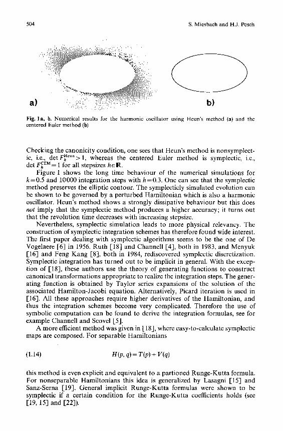
a) b)

Fig. l a, b. Numerical results for the harmonic oscillator using Heun's method (a) and the centered Euler method (b)

Checking the canonicity condition, one sees that Heun's method is nonsymplectic, i.e., detF,neu">l, whereas the centered Euler method is symplectic, i.e., det FCEM= 1 for all stepsizes heR.

Figure 1 shows the long time behaviour of the numerical simulations for k--0.5 and 10000 integration steps with h=0.3. One can see that the symplectic method preserves the elliptic contour. The symplecticly simulated evolution can be shown to be governed by a perturbed Hamiltonian which is also a harmonic oscillator. Heun's method shows a strongly dissipative behaviour but this does not imply that the symplectic method produces a higher accuracy; it turns out that the revolution time decreases with increasing stepsize.

Nevertheless, symplectic simulation leads to more physical relevancy. The construction of symplectic integration schemes has therefore found wide interest. The first paper dealing with symplectic algorithms seems to be the one of De Vogelaere [6] in 1956. Ruth [18] and Channell [,4], both in 1983, and Menyuk [16] and Feng Kang [,8], both in 1984, rediscovered symplectic discretization. Symplectic integration has turned out to be implicit in general. With the excep- tion of [,18], these authors use the theory of generating functions to construct canonical transformations appropriate to realize the integration steps. The generating function is obtained by Taylor series expansions of the solution of the associated Hamilton-Jacobi equation. Alternatively, Picard iteration is used in [16]. All these approaches require higher derivatives of the Hamiltonian, and thus the integration schemes become very complicated. Therefore the use of symbolic computation can be found to derive the integration formulas, see for example Channell and Scovel [5].

A more efficient method was given in [-18], where easy-to-calculate symplectic maps are composed. For separable Hamiltonians

(1.14) H(p, q)= T(p)+ V(q)

this method is even explicit and equivalent to a partioned Runge-Kutta formula. For nonseparable Hamiltonians this idea is generalized by Lasagni [15] and Sanz-Serna [19]. General implicit Runge-Kutta formulas were shown to be symplectic if a certain condition for the Runge-Kutta coefficients holds (see [19, 15] and [-22]).


Picking up bo th ideas, the a p p r o a c h using genera t ing funct ions is c o m b i n e d with the R u n g e - K u t t a technique in the present paper . The p a p e r is a shor t vers ion of the more de ta i led d i p l o m a thesis [17].

2 Symplectic integration via generating functions

In this sect ion we prov ide the cons t ruc t ive tools to a p p r o x i m a t e the H a m i l t o n i a n flow

z(tj+ 1)-~- gh(z(tj))

by a canonica l t r ans fo rma t ion F h which per forms the symplec t ic in tegra t ion step

z ~ + ~ = F h ( z i ) .

A central resul t of the theory of genera t ing funct ions is the fol lowing impl ic i t r ep resen ta t ion of the H a m i l t o n i a n flow gt by the g rad ien t of a sca lar funct ion S(w, t) cal led the generating function of the Hamiltonian phase f low,

,) g t ( z ) = z + J - 1 ~ w

The genera t ing funct ion S(w, t) is a so lu t ion of the Hamilton-Jacobi equation ~

-7=H

To cons t ruc t a symplec t ic in tegra t ion m e t h o d zJ+I=Fh(ZJ), w e replace S by an easy- to -ca lcu la te a p p r o x i m a t i o n ~ a n d subs t i tue this a p p r o x i m a t i o n into the above implici t equa t ion for the flow gt. This yields an in tegra t ion scheme accord ing to the pa t t e rn of the impl ic i t r ep re sen t a t i on for the flow gt,

z J + l = z J q - J - l OS (zJq-~J+l 2 ,h

1 Sir William Rowan Hamilton has shown that the problems of mechanics, for which "the principle of living forces" - now called the principle of conservation of energy - is valid, can be reduced to the integration of a partial differential equation of the first order. These results appeared first in the Philosophical Transactions 1834 and 1835 [11, 12]. In 1837 Carl Gustav Jacob Jacobi [14] levels a criticism at Hamilton's work, since Hamilton actually defines one function by two partial differential equations of the first order without showing that such a function really exists. Moreover, Hamilton's results exclude the important case where the "force-function" - later it was called the "potential function" by Gaul3 - contains the time explicitly. Jacobi: Hamilton scheint mir dadurch seine sch6ne Entdeckung in ein falsches Licht gesetzt zu haben, ausserdem dass sie dadurch zu gleicher Zeit unn6thig complicirt und beschrdnkt wird. The generalization of the Hamilton-Jacobi equation to more general problems of the calculus of variations was suggested by Eugenio Beltrami in 1868 [2]. Carath6odory [3] : Unter diesen muff man an erster Stelle Beltrami nennen, der in mehreren wundervollen Arbeiten die Beziehungen der Flgichentheorie yon GauJ3 zu den Resultaten yon Jacobi ergrfindet hat.


where h denotes the stepsize for the numerical integration. In fact, for all choices of S one obtains canonical transformations. This will be explained by the following two theorems.

The first theorem provides a special theory of generating functions: Canoni- cal transformations sufficiently close to the identity can be implicity expressed by the gradient of a scalar function.

Theorem 2.1. Let {q~,[[t[ < T} be a family of canonical transformations Z=<p~(z) including the identity for t=0 . Then for T sufficiently small, the family can be then written in the so-called implicit gradient form ( IGF)

10S [ z + Z \ (2.1) z - Z = J - -~w ~ , t)

where S=S(w, t ) denotes a real valued function defined on N2"x] - -~ l , e2 [ , 51, ~z > O. Conversely, each sufficiently smooth function S with S (w, O) = 0 generates a family of symplectic maps by (2.1).

The function S is called the generating function of the family {~0t} of canonical transformations.

Proof We introduce a new set of variables { W, w} by the following linear relations

(2.2) W,=J(z--Z), w,=�89

For each fixed t, the variables {Z, z} are coupled by the map <Pt

(2.3) z = ~0,(z).

Therefore the new variables are also coupled by a map, say, 4),

(2.4) W= 4), (w)

which is implicitly defined by

(2.5) W= J(z - <P,(z))lw = �89 + ~,~)).

Indeed, the map 4)t is, for small Ill, at least locally well defined because of

(2.6) det ( I + ~ j ) > 0 .

This holds since the Jacobian of ~0 t tends to the identity as It[---)0 because of q~o = I.

Theorem 2.1 is now a consequence of the following equivalency for each fixed t

(2.7) ~0t is canonical iff 0r is a gradient map,


i.e., ~b~ can be written as

(2.8) w= r = ~-~Sw (w, t).

Substituting the definitions (2.2), the IGF (2.1) follows immediately. To complete the proof, the equivalency (2.7) has to be shown: Having

expressed the Jacobian of ~b t by

aw az aw az \ a z ] = 2 J I - I + ,

one can easily verify that the integrability condition for the gradient map ~b, is equivalent to the canonicity condition (1.7) for q~t:

Owl ~aw/

[]

The next theorem gives a representation of the Hamiltonian flow according to the aforementioned theory of generating functions. Note that, because of historical reasons, the generating functions S of the inverse Hamiltonian flow is used; see the proof of the following theorem.

Theorem 2.2. For sufficiently small rt], the phase flow g' of the Hamiltonian H can be written as

(2.10) aS/z+g'(z) \ g'(z)-z=J-lWw ,t)

The generating function S = S(w, t) is the solution of the following initial-value problem for the partial differential equation

OS [ 1 1 (2.11) ~ { = H ~ w + ~ d - OS~, aw] S(w, 0)=0.

Proof Consider the inverse Hamiltonian flow q~t"=g-t which throws the points z(t) back to the initial points z(O)=g-'(z(t)). Thus the image points Z of the inverse flow Z=~o~(z) are time independent. Therefore the time derivative of the corresponding IGF (2.1) becomes

(2.12) 1 x 0 2 S �9 0 0 S

z=-2J - O~w 2 z + J - z at Ow"


Substituting the right-hand side of the canonical ODE (1.2) for ~ and using j - 1 = jT__ __ j , one obtains

1 0 2 S ] T OH (3 OS (2.13) I + l j - ~w2 ] ~z (Z)=~w ~(W, t ).

1 OS By virtue of the relations (2.2) and (2.8) we have z = w + 2 J - ~ ~ww" Therefore

the right-hand side of (2.13) is just the gradient of H(z) with respect to w. Hence, we have

(2.14) 0 H _ 0 0S t3w 0w 0 t '

and the Hamilton-Jacobi equation (2.11) follows by integration and the initial condition by Theorem 2.1.

Finally, the implicit gradient from of the Hamiltonian flow (2.10) is obtained by substituting z=gt(Z) in the IGF (2.1). Because of dealing with the generating function of the inverse flow ~o t =g- t , the variables Z and z have to be inter- changed in (2.10). []

Having numerical applications in mind the following lemma will be quite useful.

Lemma 2.1. The generating function S(w, t) defined by (2.11) is antisymmetric with respect to t.

Proof From the IGF of the flow gt given in (2.10), the IGF of the inverse flow g- t acting on z(t) is obtained by replacing t by - t

(2.15) 1 OS (z(t)+g-r(z(t)) --t) g- t(z( t ))--z( t )=J- ~ w \ 2 ' "

Now we re-substitute z(t) by gt(z), which yields

, OS [gt(z)+z ) (2.16) z-g'(z)= J- ~ww ~ 2 ' t

and which obviously also represents the Hamiltonian flow. Comparing the last equation with the IGF (2.10) from Theorem 2.2, the proof is completed. []

Remark 2.1. These results are special cases of more general results of Feng Kang and Qin Meng-zhao [9]. A proof of these general results can be found in [17]. It should be mentioned that there are many different types of generating functions and associated Hamilton-Jacobi equations (see, e.g., [1]). The type of generating functions used in [-9] and in the present paper cannot be found in classical mechanics. Recall that generating functions as well as the Hamiltonian are only determined up to a constant.

We now attend to the construction of symplectic integrators. Consider the IGF representation (2.10) of the Hamiltonian flow with the generating function S obtained by solving the Hamilton-Jacobi equation (2.11). As mentioned at the beginning of this section, we replace the exact solution S(w, t) by an easy-to-


calculate approximation S(w,t) to obtain a canonical transformation z s+~ = Fa(z j) which then realizes a symplectic numerical integration step,

(2.17) , ~g[z~+zi+' )

zJ+'=zJ+J- ~w[ 2 ,h .

The integration formula (2.17) is symplectic only by the construction via the IGF. This property is not affected by the choice of S.

3 Runge-Kutta ansatz for generating functions

In this section we will specify the generating function of the symplectic integration step (2.17). If we would use the exact solution S(w, t) of the Hamilton-Jacobi equation (2.11), the integration scheme (2.17) would be exact. Since S(w, t) is not available, we search for an easy-to-calculate approximate solution S(w, t). Thereby the approximation has to be done with respect to the variable t. The time t in S(w,t) corresponds to the stepsize h. Therefore the approximation

needs to be valid only for small Itl. Feng Kang obtains S as a truncated Taylor series, with respect to t, of

the solution S of the Hamilton-Jacobi equation (see [8]). In analogy to Taylor series methods for general ODEs, this approach requires the evaluation of higher derivatives of the right-hand side, i.e., of the Hamiltonian.

To circumvent this problem, we proceed here similar to Runge-Kutta methods. The occurrence of higher derivatives can be avoided by successively inserting right-hand-side terms into each other. This principle of successive insertion is here directly applied to the desired generating function S. This idea leads to the following new Runge-Kutta-type ansatz for the generating function

(3.1) 3 (

S(w,h)=h ~=lc~iH w+hfli J - ' OH (w , a l l \ \ .= ' c~z ~ +hfl'2 J - ~ z (W))) �9

Note that this ansatz substituted into the difference scheme (2.17) generally does not lead to a Runge-Kutta method as one obtains when applying the Runge-Kutta technique directly to the canonical differential equations. Rather, the Runge-Kutta insertion technique is only applied to the generating function itself. This idea results via (2.17) in a new class of symplectic integration methods.

The coefficients ~i, fill and fli2, i= 1, 2, 3, are now determined by comparing the Taylor series expansion of (3.1) around h = 0 with the Taylor series of the exact generating function S(w, t) around t = 0 yielding

(3.2) ~k ~k

~h k~(w'O)=~S(w'O)cr for k=O, 1 . . . . . p.

The maximum obtainable value for p will be given in Sect. 4. This procedure leads to a method of the order p, i.e., gh(z)- Fh(2 ) = O(h p+ 1), which follows immediately from the implicit function theorem.

A few remarks should be made concerning the complexity of the integration schemes presented. First, the sym!~lectic integration formula (2.17) uses the gradient of the generating function S. The second derivatives of the Hamiltonian


must therefore be supplied by the user, but no higher derivatives can appear independent of the order p. Take for example Feng Kang's fourth-order formula, which requires third-order derivatives of H. On the other hand, Runge-Kutta methods don't need second-order derivatives if the nonlinear system of each implicit integration step is solved by a fixed-point iteration. Second-order derivatives, too, are involved if the simplified Newton method is used. However, the number of unknowns in the equations of an implicit s-stage Runge-Kutta scheme is s times as large as in the method based on (2.17).

4 Order conditions for the Runge-Kutta-type generating functions

The determination of the unknown coefficients in the ansatz (3.1) from the Eqs. (3.2) is based on a modified Butcher tree technique (see [17], and a subsequent paper to be published). Since the generating function is a scalar function, the derivation of the conditions for the coefficients is much easier than for vector valued Runge-Kutta formulas (see, e.g., Fehlberg [7]). One obtains fewer equations for each order condition.

The conditions are

3 3 (4.1) (I) ~, a i = l , (V.1) ~ ai(5fl~,-2Ofli , fl32)= ~ ,

i = l i = l

3 3

(III) 2 ~(3flz1-6fl,1 fl,2)=�88 (V.2) ~ 60a,(f121 fl~2-fl 3, fl~2)=�88 i = 1 i = l

3 3

(IV) ~" e~(4fl~,-12fl~lfl~2)=O, (V.3) ~ 60c~,fl~,fl~=�89 i = l i = 1

The Roman numbers in front of the equations indicate the order of the terms in the Taylor expansion. An equation corresponding to the second-order term

02~ does not appear since it turns out that ~ - vanishes for t = 0.

There are 6 equations for the 9 unknown coefficients in (3.1). Proceeding to the sixth order, 4 additional equations must be taken into account leading to an overdetermined system. However, it is possible to obtain a sixth-order method by taking advantage of the antisymmetry of S according to Lemma 2.1. A formula with coefficients satisfying all the above equations is of the sixth order if it is, in addition, antisymmetric. This is because the sixth-order derivatives of both S and ~ vanish. Moreover, the antisymmetry allows a consistency check when calculating the right-hand sides of (3.2). Formulas with orders higher than 6 can be obtained only by including more terms in a modified version of ansatz (3.1).

A special antisymmetric fourth-order formula is now presented,

( 4 . 2 ) ~(w,h)=h~, H(w)+h~ 2 H(w+hfl2 , j-x ~z (W))

OH + h ~ 2 H ( w - h f 1 2 1 J - l ~ ( w ) ) .


Note that e2 =(x3, f i l l = 0 , f131 = --fl21 and all fli2 =0. This leads to the following equations

(4.3) (I) cq + 2 c~ 2 = 1,

(III) 6ct 2 fiE 1 =�88

(v.1) lOc, / L

with the solution ~1 = 4/9, ~2 = 5/18 and fl21= ]//3-/20. Because of the antisymmetry no equation for the fourth-order term (IV)

appears, and a double insertion is not required in the ansatz (3.1). The third equation (V.1) is included here in order to reduce the truncation error

1 /Os~ r S ,~ (4.4) TE.'=~- ~ h = O ~ ,=0}"

Equation (V.1) assures that the term with the highest derivative of the Hamilton- Jan disappears in TE; this term is expected to make the largest contribution to the truncation error.

Inserting the special generating function S from (4.2) into the symplectic integration formula (2.17), we end up with the following integration scheme 2

zj+ 1 = z./+ h {~1 b + oc2 (b + + b - ) _ h ~ 2 fl21 A( b+ - b - ) } (4.5)

with (z , + z, + ,1

b = J - ' \ -2 ),

b e : = J - d z \ 2 +hf121J- ~zz \ 2 '

A , = J - Oz 2 ]"

An additional fourth-order method and two fifth-order methods are given in [17]. They are discussed with respect to their amount of computation, their truncation errors and their dependence on roundoff errors. In that paper also a pair of symplectic integration methods of the orders 4 and 5, respectively, is presented which allows to estimate the error and to control the stepsize similar to Runge-Kutta-Fehlberg methods. Alternatively one can also develop an error estimate based on the preservation of energy, i.e., of the Hamiltonian, of the problem. Despite of more precise results when applying methods with built-in error estimates, these methods, however, cannot preserve the qualitative behaviour of the solutions in long time simulations. The symplectic integration of a canonical system with Hamiltonian H can be shown to be formally equivalent to the exact integration of, again, a canonical system with a l~erturbed Hamilton- ian/4. This Hamiltonian depends on the stepsize used, i.e., H(z)=/~ (z; h). There- fore a stepsize-controlled integration is governed by Hamiltonians /4 varying from step to step. The qualitative performance of a variable-step symplectic

2 In his doctoral thesis [21] Stoffer independently developed the same integration method as in (4.5) in a completely different way.


method is comparable to the performance of a variable-step Runge-Kutta method.

To conclude this section, we want to summarize some properties of the method (4.5) concerning stability. First, the stability function of the method is given by

24+ 122-23 (4.6) ~(2) - 2 4 - 122 + 23.

For linear canonical systems it is known (see Feng-Kang [8]) that the condition

(4.7) ~ (2) O ( - 2) - 1

is equivalent to the symplecticity of the method associated with ~. This condition results for linear canonical systems in the preservation of all quadratic invariants including the Hamiltonian; see [8], too. Second, it can easily be shown that every symplectic integration formula for which a stability function ~ exists is P-stable, thus preserving harmonic oscillations. For the definition of P-stability see Hairer [10]. In summary, symplecticity is equivalent to P-stability for linear canonical systems. However, even A-stability (see, e.g., [20], p. 464) is not sufficient for symplecticity in the gernal nonlinear case; see again [8].

5 Numerical evaluation of the integration step

The implicit symplectic integration step (2.17) must be evaluated iteratively, which is carried out by an appropriate fixed-point iteration. Using the definitions

zJ+ z j+l O ( w , h ) : = l j - 1 ~?S (5.1) x : = ~ , ~w(W, h),

the symplectic integration step (2.17) takes the form of a fixed-point equation

(5.2) x = z J+ O(x , h).

Then z ~+ 1 is obtained from x by

(5.3) z j + 1 = 2 x - z ~.

Since the Lipschitz constant of (5.2) is, because of (3.1) and (5.1), of the first order in the stepsize h, the fixed-point iteration seems to be appropriate for the numerical solution. Hence, we can iterate

(5.4) x l + l = z J + O ( x t , h), /=0, 1 . . . . , with x ~


Note that the application of the fixed-point iteration avoids the evaluation of third-order derivatives of H as it would be needed, e.g., for the simplified Newton method.

The following Lemma shows that for a p-th-order integration scheme only p iterations have to be performed. Note that in this case the symplectic invariants are only preserved up to the order p + 1.

Lemma 5.1. The I-th iterate xt=xl(h) approximates the solution x= x (h ) of (5.2) to the order I:

(5.5) xZ (h)- x(h)= O(h l+ 1).

Proof The Lemma can be easily verified by induction. []

With some modifications the amount of computat ion for the fixed-point iteration can be reduced considerably. This is based on the following

Lemma 5.2. I f Yct denotes any approximation of the order l for the solution x,

i.e., 2 t - x = O ( h t + i ) , one obtains an approximation x I+~ of the order l + l by (5.4) even in the case the iteration step is evaluated only up to the order l+2 . This means

(5.6) x'--~+~:=zJ+O(s with ~)=O+O(h'+2).

Proof The proof follows the line of the proof of Lemma 5.1. []

We can now reduce the amount of computat ion as follows:

1. According to Lemma 5.1 the first two iteration steps can be performed using a second-order generating function, for example, the generating function of the centered Euler method (1.12),

(5.7) S(w, h)= hH(w).

This is sufficient to obtain a starting value of the second order for the iteration of the fourth-order method. 2. The expensive evaluations of the second-order derivatives of H can be mini- mized as follows: If the second derivatives of H appear in the iteration in a term of the r-th order, i.e.,

xl+t . . . . + O ( h r ) j - t 6~2H" l TzT(X + . . .)+ ....

one can replace the iterate x z by a preceeding iterate, say, x t-m as long as m < r - 1. Indeed, since x l - x l - " = O(h t-"+ 1), a perturbat ion of the order

r + ( l - - m + l )> l+ 2


is introduced into the term O of the iteration. Therefore Lemma 5.2 guarantees that the ( l+ 1)-st iterate remains of the order l+ 1 if the second derivatives of H are evaluated only every m + 1 iteration steps.

For the integration scheme (4.5) these two modifications are explained in more detail by the following algorithm:

X 0 :~_ Z j

h 1 ~l t(xo ) xl '=z +-2 J - ~z

h 1 ~H(xx ) X 2 : = Z J § J - 6~ z

l.'=2

repeat

s h x '+ ' . . = z + ~ { ~ , blx,+C~z(b+lx, +b-Ix,)-h~2 f12, A(b+l~,--b-[x,)}

with A .'--AI~, updated only i f /= 2, 5, 8 ....

l : = / + l

until numerical convergence.

The first two steps are based on the centered Euler method. In the loop the second-order derivatives A of H have to be evaluated every third step according to Item 2. This is because the second-order derivatives appear in a third-order term in (4.5). Note that in (4.5) the difference b + - b - is already of the first order.

According to Lemma 5.1 one has to carry out 2 loops to obtain a fourth- order approximation when neglecting the full preservation of the symplecticity. In this case, the number of function evaluations runs up to 8 calls of the right-

hand side J - 1 aH and only one additional call of the Jacobian J - 1 t~2Ht3z2. How-

ever, we will see in Sect. 6 that only an iteration up to full machine precision will give all the advantages of symplectic integration.

6 Numerical results

In this section we describe some numerical experiments to show the performance of symplectic integration by comparing the fourth-order symplectic method of this paper with the classical fourth-order Runge-Kutta method (see, e.g., [20], p. 414).

First we consider a planar pendulum with Hamiltonian

(6.1) H(p, q)= �89 p2 --COS q.


Fig. 2. Numerical results for the planar pendulum using the classical fourth-order Runge-Kutta method (left), a "reduced symplectic" method (middle) and the fourth-order symplectic method (right)

Figure 2 shows the phase portrait of a libration of the pendulum for initial values p(0)=0 and q(0)= 3.1. The right figure shows the result of the symplectic integration whereas on the left we have the result of the Runge-Kutta method. These results were obtained after 50000 integration steps of length h=0.3. We have seen in Sect. 1 that in the linear case the contour is preserved exactly since it is a level line of the preserved quadratic Hamiltonian (see also the remarks at the end of Sect. 4). In the nonlinear case, however, the energy can be preserved only approximately. Nevertheless, even in the nonlinear case the symplectic simulation yields a clear-cut contour. This contour deviates from the exact level lines far below drawing accuracy. The nondissipative behaviour of the pendulum is unchanged by the symplectic simulation. This is independent of the number of integration steps and the stepsize. In contrast, the Runge-Kutta method cannot reproduce any contour; the phase portrait collapses. The behaviour is dissipative.

The middle part of Fig. 2 shows the result of the "reduced symplectic" simulation. That is, the integration steps are numerically evaluated only within an accuracy given by the order according to Lemma 5.1. All properties of symplectic integration get lost. Consequently, the implicit equations must be evaluated up to full machine precision.

The second example describes the motion of a star in an axisymmetric galaxy. The example is well-known in the literature as the H6non-Heiles system (see H6non and Heiles [-13]). By virtue of axisymmetry the problem can be reduced to a planar movement governed by the following Hamiltonian

(6.2) H ( p , , p 2 , q , , q 2 ) = � 8 9 2 1 2 Pz)+~(ql +q~ 2 2 3 + 2 q l q2--xq2).

Instead of pursuing a complete trajectory, H6non and Heiles considered its points of intersection with a certain two-dimensional surface within the corresponding three-dimensional energy-level surface. This surface o f sections can be parameterized by the coordinates P2 and q2- Two cases have to be distin- guished. Depending on the energy level, the points of intersection are either on a curve or lie densely within an open subset of the surface of sections. The first case indicates the existence of a second isolated integral in addition to the first integral H. Indeed, the trace of its level surface is just the above


mentioned curve on the surface of sections. In the second case, no further isolated integral can exist.

First, we discuss the low energy behaviour (H= 1/2). Figure 3 shows the points of intersection of two distinct trajectories.

The first trajectory is marked by diamonds (<>), the second trajectory by circles (o). The initial point of the first trajectory is situated at the crossing point in the middle of the two figures. The trace of the second trajectory splits into two parts. The pear-shaped part is intersected from behind, the banana- shaped part from the front side. The initial point of the second trajectory is situated on the pear-shaped contour. The pictures are obtained after 50000 integration steps of length h--0.1 using either the symplectic method (top) or the classical Runge-Kutta method (bottom). The points of intersection of both trajectories lie on curves, thus the low energy state represents a case where a second isolated integral exists. Obviously, this behaviour is reproduced by both methods equivalently. Nevertheless, one important difference can be observed. For the symplectic simulation, there is only a finite number of intersection points for the second trajectory, which are passed periodically. This behaviour gets lost when using the classical Runge-Kutta method unless a considerably reduced stepsize is used. Even in that case, however, the periodicity will disappear for an increasing number of integration steps.

The picture is different for high energy. Doubling the energy to H = 1/6 changes the behaviour dramatically. The motion becomes chaotic. The symplectic simulation in Fig. 4 (top) shows the trace of a single trajectory only. The intersection points tend to fill densely a region on the surface of sections. So a second isolated integral seems not to exist. Using the classical Runge-Kutta method the qualitative behaviour is completely destroyed. Both results are obtained after 30000 integration steps of length h = 0.5. To get meaningful results with the Runge-Kutta method the stepsize has to be reduced to h = 0.125 requir- ing then 120000 steps. This result and an intermediate simulation with 60000 steps of size h = 0.25 are shown in Fig. 5.

The most important advantage of symplectic integration is that the qualitative behaviour of the trajectories can be obtained independent of the number and the size of the integration steps.

Again we want to emphasize that symplecticity does not result in a higher accuracy compared to nonsymplectic integration. Especially for simulations of chaotic motions, a high accuracy is neither obtainable nor meaningful. All that matters is that the approximate phase flow Fh has the same qualitative properties as the underlying Hamiltonian flow g', for example, ergodicity properties and invariant integrals.

8 Conclusions

The present paper has shown that symplectic integration methods are superior on investigating the qualitative behaviour of Hamiltonian systems, in particular, when long time simulations are to be performed. For that purpose a new class of symplectic integration schemes has been developed. These methods turn out to be not only efficient but, because of their construction via generating functions, they are closely related to the canonical theory.


o

o

~o

o

o

�9 ~ ooo o ".,

2 1 ~" o . . . . . o "~ o + .~ ~ 1 7 6 o o o o

o ,~'~~ o o ~ ~ *. o | , o ~ o '~ o ~ s ~ o~ o +

o o �9

o ~ o it o . ~ o o

o ~ ", %Oo oO~ o ~ "~'"- �9 ~ 1 7 6 1 7 6 1 7 6 4 #

o o , , - ~ .

o ~ ~"~~ ,,~ o ~ : ~ ~ ~ o

o I o o oOc~ ..

\

Fig. 3. Numerical results for the Hbnon-Heiles system at low energy (H = 1/12) using the fourth- order symplectic method (top) and the classical fourth-order Runge-Kutta method (bottom)


�9 + ~++ .+

�9 . " : . . . " . .

�9 . . . . . ;..'.+ tP"

. , \ . 7 : + : + " . . . . . .~. . : . . " 5 " ' - : +

. . . . .. . . :o ~ ~,d~ . . . + . : . .

�9 . + + . + ~ + ~ R I �9 " " + �9 �9 + . . . . . ' + + . . + . , + , +,. �9 �9 �9 �9 + " . ' ~ r . ~ + ~ . ' . ' . " : ' " �9 ":

.+ .:+, ; . ; + ~ . s + ~ . ~ . - . . . . . : . : . . . .

�9 +" + " " ~ k " ~ + + , ; , : ~ " ++'+.. " �9 o+,+++ �9 ++,+<+:'~. + o+++. + + o

++ + :. ++ ++.++~+ + �9 . + + + ++. ++t+ +

+~ " � 9 +4+

. + " + ' ; ; : + .

. : ' , �9

Fig. 4. Numerical results for the H6non-Heiles system at high energy (H = 1/6) using the fourth- order symplectic method ( t o p ) and the classical fourth-order Runge-Kutta method ( b o t t o m )

Symplectic phase flow approximat ion for the numerical integration 519

tz*" . .Z" . g . . . ~-

. .~ o"., �9 �9 .~. ..-r ~ *.7,,~'~-7.~_.*,.r ; ' r . ~ . .

. . . , ~ , ~ . ~ : . . . . . . . . . . . �9 . ~ . � 9 4t, ~ . �9 #~ ~ ~ �9 ,g,,,..- ~ ~ �9

Fig. 5. Numerical results for the H6non-Heiles system at high energy (H = 1/6) using the classical four th-order Runge-Kut ta me thod with halfed (top) and quartered (bottom) stepsize


Acknowledgements. The authors would like to thank Professor R. Bulirsch and Professor P. Rentrop for their support and fruitful discussions and Professor D.R. Smith for checking the English of the manuscript. They are indebted to Professor Feng Kang for inspiring this work by his lecture in January 1988 at Munich University of Technology. They also want to thank Professor J.M. Sanz-Serna and Dr. D. Stoffer for their helpful comments on a previous version of this paper.

References

1. Arnol'd V.I. (1978): Mathematical Methods of Classical Mechanics. Springer, Berlin Heidel- berg New York

2. Beltrami, E. (1868/1902-20): Sulla teoria delle linee geodetiche. Rendiconti del Reale Istituto Lombardo (serie I1) 1, 708 718 (1868) = Beltrami, E. : Opere Matematiche 1,366 373. Hoepli, Milano (1902-1920)

3. Carath6odory, C. (1935): Variationsrechnung und partielle Differentialgleichungen erster Ordnung. Teubner, Leipzig

4. Channetl, P.J. (1983): Symplectie Integration Algorithms. Internal Report AT-6: ATN-83-9. Los Alamos National Laboratory, Los Alamos

5. Channell, P.J., Scovel, C. (1990): Symplectic Integration of H amiltonian Systems. Nonlinear- ity 3, 231-259

6. De Vogelaere, R. (1956): Methods of Integration which Preserve the Contact Transformation Property of the Hamiltonian Equations. Report No. 4. Department of Mathematics, Univer- sity of Notre Dame, Notre Dame, Ind.

7. Fehlberg, E. (1970): Low-Order Classical Runge-Kutta Formulas with Stepsize Control and Their Application to Some Heat Transfer Problems. Computing 6, 61-71

8. Feng Kang (1985): On Difference Schemes and Symplectic Geometry. In: Feng Kang, ed., Computation of Partial Differential Equations. Proceedings of the 1984 Beijing Sympo- sium on Differential Geometry and Differential Equations, pp. 42-58. Science Press, Beijing

9. Feng Kang, Qin Meng-zhao (1987): The Symplectic Methods for the Computation of Hamil- tonian Equations. In: Zhu You-lan, Guo Ben-yu, eds., Numerical Methods for Partial Differential Equations. Proceedings of a Conference held in Shanghai, 1987. Lecture Notes in Mathematics, Vol. 1297, pp. 1-35. Springer, Berlin Heidelberg New York

10. Hairer, E. (1979): Unconditionally Stable Methods for Second Order Differential Equations. Numer. Math. 32, 373379

11. Hamilton, W.R. (1834/1931-40): On a General Method in Dynamics by Which the Study of the Motions of All Free Systems of Attracting or Repelling Points is Reduced to the Search and Differentiation of One Central Relation, or Characteristic Function. Philosophi- cal Transactions of the Royal Society 124, 247 308 (1834)=A.W. Conway, J.L. Synge, eds., The Mathematical Papers of Sir William Rowan Hamilton, Vol. 2, pp. 103 167. Cam- bridge University Press, Cambridge (1931 1940)

12. Hamilton, W.R. (1835/1931-40): Second Essay on a General Method in Dynamics. Philoso- phical Transactions of the Royal Society 125, 95-144 (1835)=A.W. Conway, J.L. Synge, eds., The Mathematical Papers of Sir William Rowan Hamilton, Vol. 2, pp. 162 216. Cam- bridge University Press, Cambridge (1931-1940)

13. H6non, M., Heiles, C. (1964): The Applicability of the Third Integral of Motion: Some Numerical Experiments. Astron..J. 69, 73 79

14. Jacobi, C.G.J. (1837/1881-91): Uber die Reduction der Integration der Partiellen Differen- tialgleichungen erster Ordnung zwischen irgend einer Zahl Variablen auf die Integration eines einzigen Systemes gew6hnlicher Differentialgleichungen. Crelle Journal ffir die reine und angewandte Mathematik 17, 97-162 (1837)=K. Weierstrass, ed., C.G.J. Jacobi's Gesam- melte Werke, Vol. 4, pp. 57 127. Reimer, Berlin (1881-1891)

15. Lasagni, F.M. (1988): Canonical Runge-Kutta Methods. ZAMP 39, 952 953 16. Menyuk, C.R. (1984): Some Properties of the Discrete Hamiltonian Method. Physica D

11, 109-129 17. Miesbach, S. (1989): Symplektische Phasenflul3approximation zur numerischen Integration

kanonischer Differentialgleichungen. Diploma Thesis, Department of Mathematics, Univer- sity of Technology, Miinchen


18. Ruth, R. (1983): A Canonical Integration Technique. IEEE Trans. Nucl. Sci. 30, 266~2671 19. Sanz-Serna, J.M. (1988): Runge-Kutta Schemes for Hamiltonian Systems. BIT 28, 877-883 20. Stoer, J., Bulirsch, R. (1980): Introduction to Numerical Analysis. Springer, Berlin Heidel-

berg New York 21. Stoffer, D.M. (1988): Some Geometric and Numerical Methods for Perturbed Integrable

Systems. Dissertation, Department of Mathematics, Swiss Federal Institute of Technology, Zfirich

22. Suris, Y.B. (1988): On the Preservation of the Symplectic Structure in the Course of Numeri- cal Integration of Hamiltonian Systems. In: S.S. Filippov, ed., Numerical Solution of Ordi- nary Differential Equations, pp. 148-160. Keldysh Instiute of Applied Mathematics, USSR Academy of Sciences, Moscow [in Russian]

Symplectic phase flow approximation for the numerical ... · Symplectic phase flow approximation...

Documents

Transcript of Symplectic phase flow approximation for the numerical ... · Symplectic phase flow approximation...