Symmetries of differential equations

Libor SnoblDepartment of Physics, Faculty of Nuclear Sciences

and Physical Engineering, Czech Technical University in Prague

Lectures presented at Instituto de Matematica Interdisciplinar(IMI) y el Departamento de Geometrıa y Topologıa,

Facultad de CC Matematicas, UCM,

January 9 – January 19, 2012

Abstract

The purpose of this short course is to introduce the concept of pointsymmetries of differential equations. Next, we shall use point symme-tries to solve a given ordinary differential equation. The method isbased on finding a suitable transformation of independent and depen-dent variables after which we can reduce the order trivially. We shallalso briefly indicate other applications.

1

Contents

1 Definition of Lie group and its Lie algebra 3

2 Actions of Lie groups 5

3 Symmetries of algebraic equations 7

4 Symmetries of differential equations 10

5 Applications: Reduction of the order of a given ODE andothers 19

Index 26

References 27

2

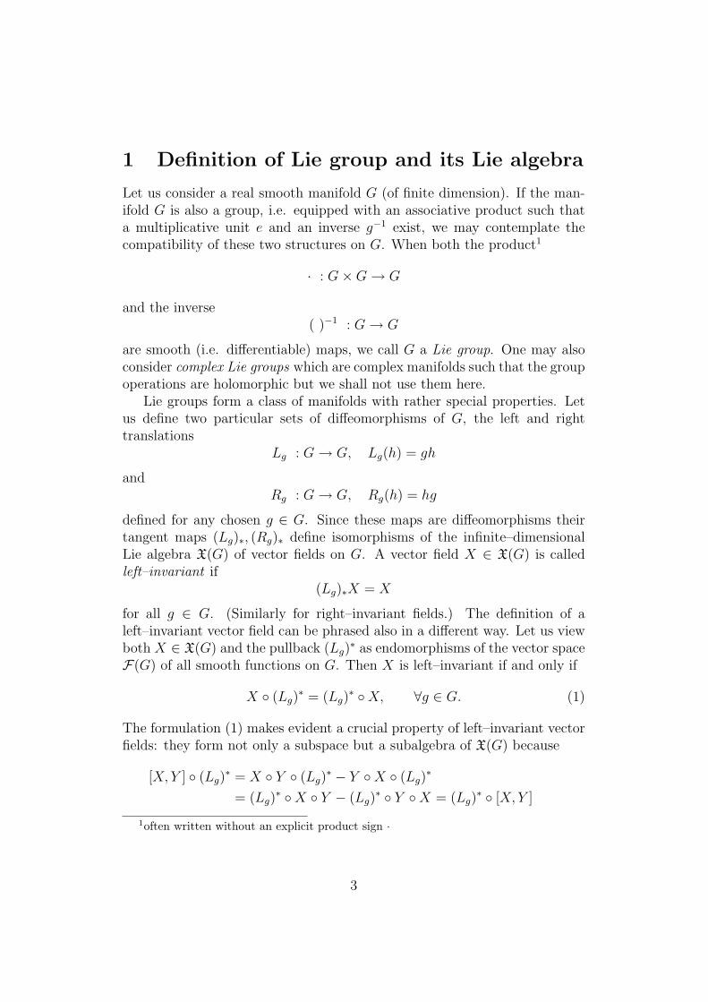
1 Definition of Lie group and its Lie algebra

Let us consider a real smooth manifold G (of finite dimension). If the man-ifold G is also a group, i.e. equipped with an associative product such thata multiplicative unit e and an inverse g−1 exist, we may contemplate thecompatibility of these two structures on G. When both the product1

· : G×G→ G

and the inverse( )−1 : G→ G

are smooth (i.e. differentiable) maps, we call G a Lie group. One may alsoconsider complex Lie groups which are complex manifolds such that the groupoperations are holomorphic but we shall not use them here.

Lie groups form a class of manifolds with rather special properties. Letus define two particular sets of diffeomorphisms of G, the left and righttranslations

Lg : G→ G, Lg(h) = gh

andRg : G→ G, Rg(h) = hg

defined for any chosen g ∈ G. Since these maps are diffeomorphisms theirtangent maps (Lg)∗, (Rg)∗ define isomorphisms of the infinite–dimensionalLie algebra X(G) of vector fields on G. A vector field X ∈ X(G) is calledleft–invariant if

(Lg)∗X = X

for all g ∈ G. (Similarly for right–invariant fields.) The definition of aleft–invariant vector field can be phrased also in a different way. Let us viewboth X ∈ X(G) and the pullback (Lg)

∗ as endomorphisms of the vector spaceF(G) of all smooth functions on G. Then X is left–invariant if and only if

X ◦ (Lg)∗ = (Lg)

∗ ◦X, ∀g ∈ G. (1)

The formulation (1) makes evident a crucial property of left–invariant vectorfields: they form not only a subspace but a subalgebra of X(G) because

[X, Y ] ◦ (Lg)∗ = X ◦ Y ◦ (Lg)

∗ − Y ◦X ◦ (Lg)∗

= (Lg)∗ ◦X ◦ Y − (Lg)

∗ ◦ Y ◦X = (Lg)∗ ◦ [X, Y ]

1often written without an explicit product sign ·

3

for any left–invariant vector fields X, Y . The algebra of left–invariant vectorfields is called the Lie algebra of the Lie group G and denoted by g.2

Elements of g are uniquely specified by their value at any chosen pointg ∈ G. Conventionally, this identification is performed at the group unit, i.e.we identify

g ' TeG.

Therefore, the dimension of g is the same as dimension of the Lie group G.One of the properties of left–invariant vector fields is that they are com-

plete, i.e. any integral curve γ(t)

γ(t) = X(γ(t))

of X ∈ g can be extended to all real values of the curve parameter t ∈ R.This property allows us to define the exponential map from the Lie algebrato the Lie group

exp : g→ G : X → γX(1) where γX(t) = X(γX(t)), γX(0) = e. (2)

The exponential map is a local diffeomorphism of g into G, i.e. is smoothand is a diffeomorphism of some open neighborhood U of 0 ∈ g onto the openneighborhood exp(U) of e ∈ G.

Using the exponential map one may relate properties of Lie groups andtheir Lie algebras. In essence any local property of Lie groups has its coun-terpart in the properties of Lie algebras. Therefore, one may say that locally,i.e. up to topological issues, a Lie group and its Lie algebra encode thesame information. Because Lie algebras are vector spaces, most computa-tions in the theory of Lie algebras reduce to problems of linear algebra andconsequently are much easier to handle than the corresponding computation

2More generally, an abstract Lie algebra g is a vector space over a field F equippedwith a multiplication (also called a bracket), i.e. a bilinear map [ , ] : g× g→ g, such that

[y, x] = −[x, y] (antisymmetry)0 =

[x, [y, z]

]+[y, [z, x]

]+[z, [x, y]

](Jacobi identity)

for all elements x, y, z ∈ g. In what follows we shall consider the fields F = R, C andfinite–dimensional Lie algebras only.

The structure of the Lie algebra g can be represented in any chosen basis (ej)dim gj=1 by

the corresponding structure constants cjkl in the basis (ej)dim g

j=1

[ej , ek] =dim g∑l=1

cjklel.

4

in Lie groups. Therefore, using the local diffeomorphism exp (2) one maysolve many problems on Lie groups which would be intractable on a generalsmooth manifold (or on a general, e.g. discrete, group).

2 Actions of Lie groups

For applications in both mathematics and physics we need a formalism allow-ing us to view Lie groups as sets of certain transformations of some objects.This leads us to the notion of an action of the group.

A (left) action of the Lie group G on a manifold M is a smooth map

. : G×M →M : (g,m)→ g . m

such that g1 . (g2 .m) = (g1g2) .m and e .m = m for all g1, g2 ∈ G, m ∈M .Similarly one may consider also right actions / : M × G → G which

satisfy (m / g1) / g2 = m / (g1g2) and m / e = m. Any left action . defines aright action / through m / g = g−1 . m and vice versa.

An action . of G on M is called effective if for every g ∈ G differentfrom the group unit e an element m ∈ M exists such that g . m 6= m.Consequently, we can reconstruct the group multiplication on the group Gfrom the knowledge of its effective action.

Examples of left actions of the group G on itself are

g . h = gh, g . h = h · g−1

and the adjoint action

Ad : G×G→ G : Adg(h) ≡ Ad(g, h) = g · h · g−1.

When the manifold M is a vector space and the action of G on M islinear

g . (av + w) = a(g . v) + g . w, ∀g ∈ G, v, w ∈M,a ∈ R

it is equivalent to a representation of the group G on the vector space M . Arepresentation of the Lie group G on a vector space V is any (smooth) map

ρ : G→ End(V )

which satisfies

ρ(e) = 1, ρ(g1g2) = ρ(g1) ◦ ρ(g2), ∀g1, g2 ∈ G.

5

A representation can be associated to any linear action by the prescription

ρ : G→ End(M) : ρ(g)v = g . v.

Whether we speak about a linear action or a representation is just amatter of convenience in the problem at hand.

A particular representation of the Lie group G on its algebra g is definedby the derivation of the adjoint action

Ad : G→ gl(g) : Ad(g) = (Adg)∗.

This representation is called the adjoint representation of G.Further differentiating we get the adjoint representation of the Lie algebra

g on itselfad : g→ gl(g) : ad = Ad∗.

It can be shown that the adjoint representation of the Lie algebra satisfies

ad(x) y = [x, y] (3)

for any pair x, y of elements of g.Sometimes we may encounter actions which are not well–defined for all

pairs (g,m). Formally, one defines a local (left) action of a Lie group Gon a manifold M to be a smooth map . : U → M where U is some openneighborhood in G×M which contains the whole subset {e}×M and satisfiesthe properties

e . m = m, ∀m ∈Mand

g1 . (g2 . m) = (g1g2) . m

whenever (g2,m) and (g1, g2 . m) ∈ U .When we consider an abstract Lie group G together with its prescribed

(local) effective action on some manifold M we often speak about a (local)group of transformations or group of motions of M . In fact, this notion waswhat Sophus Lie had in mind in his pioneering works [1, 2, 3, 4] on what wenow call Lie groups and Lie algebras.

An infinitesimal action of the Lie algebra g on M is a homomorphismµ : g → X(M). We often write the image of x ∈ g in capital letters,µ(x) ≡ X. A Lie algebra equipped with an injective infinitesimal action onsome manifold M is called an algebra of infinitesimal transformations.

Any local action of G on M gives rise to an infinitesimal action of the Liealgebra g on M through the prescription

(µ(x)f) (m) =d

dt

∣∣∣∣t=0

f (exp(tx) . m) , ∀f ∈ F(M),m ∈M. (4)

6

3 Symmetries of algebraic equations

Now we shall introduce the notion of a symmetry of a given equation. Next,we apply it in particular to differential equations. Again we present only theessential notions and ideas. For proofs see [5, 6].

Letf(x) = 0, f : Dom(f) ⊂ FN → FN (5)

be a system of algebraic equations (or just one equation when N = 1) andSf be its solution set

Sf = {x ∈ Dom(f) |f(x) = 0}.

A symmetry of the equation (5) is any transformation

T : Dom(f)→ Dom(f)

such that it preserves the solution set

T (Sf ) = Sf . (6)

Usually, we restrict our attention to transformations T which are diffeomor-phisms, T ∈ Diff(Dom(f)).

It follows from the definition of a symmetry that symmetries of a givenequation form a group, i.e. a subgroup of Diff(Dom(f)). Let us denote thisgroup of symmetries of the equation (5) by Sym(f = 0).

The group of all diffeomorphisms Diff(Dom(f)) is infinite–dimensional.While the use of the theory of Lie algebras as introduced above is not com-pletely rigorous in this case, we may in a certain sense view the algebraX(Dom(f)) of vector fields on Dom(f) as a Lie algebra of Diff(Dom(f)).When Sym(f = 0) happens to be a a Lie group (more precisely, a Lie groupof transformations), the corresponding algebra sym(f = 0) of infinitesimaltransformations defines a subalgebra of X(Dom(f)). Its relation to the func-tion f is derived using the notion of a 1–parameter subgroup.

A 1–parameter subgroup σ of a group G is a homomorphism of the ad-ditive group (R,+) into the group G. While G may not necessarily be aLie group (cf. Diff(Dom(f))), the image σ(R) has a natural structure of a1–dimensional Lie group (or 0–dimensional if σ(t) = e for all t ∈ R). Conse-quently, one may consider its Lie algebra. When G is a group of transforma-tions of M and σ its 1–parameter subgroup we have a 1–dimensional algebraof infinitesimal transformations spanned by its generator Xσ ∈ X(M):

Xσj(m) =d

dt

∣∣∣∣t=0

j (σ(t) . m) , ∀j ∈ F(M).

7

Let Sym(f = 0) be the group of symmetries of the equation (5). Weshall call the vector subspace of X(Dom(f)) spanned by all generators Xσ of1–parametric subgroups of the group Sym(f = 0) the algebra of infinitesimalsymmetries of the equation f = 0 and denote it by sym(f = 0). It turnsout that sym(f = 0) is a subalgebra of X(Dom(f)). The algebra sym(f = 0)coincides with the algebra of infinitesimal transformations arising from thegroup of transformation Sym(f = 0) when Sym(f = 0) is a Lie group.

Let us take m ∈ Sf and Xσ ∈ sym(f = 0). Because σ(t) lies in thesymmetry group Sym(f = 0) for all t ∈ R we have f(σ(t) . m) = 0 andconsequently

Xσf(m) =d

dt

∣∣∣∣t=0

f (σ(t) . m) = 0.

That means that the vector fields X in the algebra of infinitesimal symmetriessym(f = 0) of the equation f = 0 satisfy

Xf∣∣f=0

= 0, i.e. Xf(m) = 0, ∀m ∈ Sf . (7)

Let us consider the converse problem. We recall that the flow of the vectorfield X is the map

ΦX : U →M : ΦX(0,m) = m,d

dtΦX(t,m) = X(ΦX(t,m)), ∀(t,m) ∈ U,

(8)where U is some open neighborhood U ⊂ R×M such that (0,M) ⊂ U .

Let X ∈ X(Dom(f)) satisfy the condition (7). Is it true that the flow ΦX

defines a 1–parameter group of symmetries of the equation (5)?In general, the answer is negative for two reasons.Firstly, the flow may not be defined on the whole R × Dom(f), i.e. the

vector field may not be complete. That is why we introduced the notion ofa local action of a group: the flow of a vector field defines in general a localaction of a 1–parameter group.

Secondly, even locally the flow may not define symmetries of the givenequation (5).

Example 1 Let us consider a system of equations

x1 − x22 = 0, x1 = 0. (9)

Its set of solutions is S = {(0, 0)}. On the other hand, the condition (7) issatisfied by the vector field

X = ∂x2

8

whose flow is

ΦX : R× (R× R)→ (R× R) : ΦX(t, x1, x2) = (x1, x2 + t).

Now the action of the group element t 6= 0, ΦX(t, ·), takes the solution (0, 0)to a point (0, t) which is not a solution of the equation (9).

It turns out that the condition on the function f which prevents such patho-logical behaviour is the maximality of the rank of the Jacobian, rank

∂fj

∂xk

∣∣Sf

=

N . These results are the content of

Theorem 1 (On infinitesimal generators of symmetries) Let

f : Dom(f) ⊂ RN → RN define a system of equations

f(x) = 0 (10)

such that

rank∂fj∂xk

(x) = N , ∀x ∈ Sf . (11)

Then a vector field X ∈ X(Dom(f)) generates a local 1–parameter group ofsymmetries of the equation (10) if and only if

(Xf)(m) = 0, ∀m ∈ Sf . (12)

We see that under the assumption of regularity of the function f (11) we candetermine the algebra of infinitesimal symmetries sym(f = 0) of the givenequation f = 0 through solution of a linear system of equations (7) for thecoefficient functions X i ∈ F(Dom(f)) of the vector field

X : X(x) =N∑i=1

X i(x)∂

∂xi

∣∣∣∣x

.

Infinitesimal symmetries can be converted into actual symmetries throughcomputation of the corresponding flows; composing the flows one may con-struct a local group of symmetries of the given equation f = 0. In thisway, the description of infinitesimal symmetries in terms of the condition (7)significantly simplifies the search for symmetries of the given equation.

Detection of symmetries which cannot be connected to identity trans-formation by flows of infinitesimal symmetries, e.g. belonging to differentconnected components of the symmetry group, is a much harder problemand we shall not discuss it here.

9

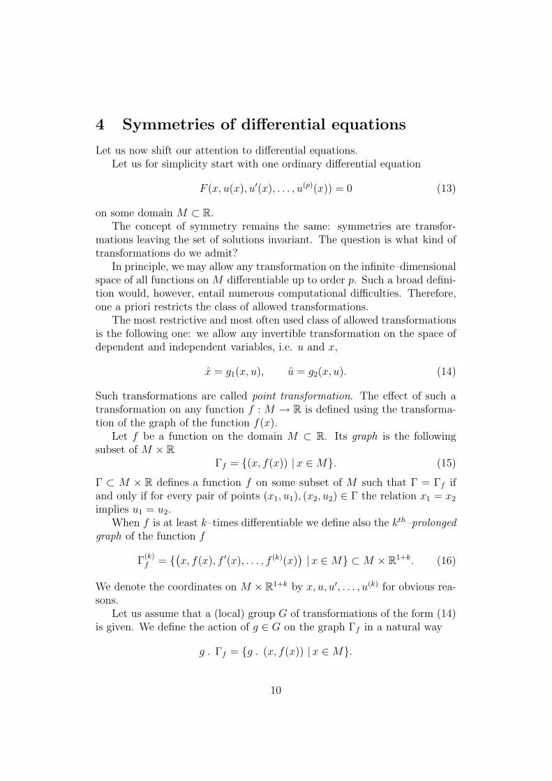
4 Symmetries of differential equations

Let us now shift our attention to differential equations.Let us for simplicity start with one ordinary differential equation

F (x, u(x), u′(x), . . . , u(p)(x)) = 0 (13)

on some domain M ⊂ R.The concept of symmetry remains the same: symmetries are transfor-

mations leaving the set of solutions invariant. The question is what kind oftransformations do we admit?

In principle, we may allow any transformation on the infinite–dimensionalspace of all functions on M differentiable up to order p. Such a broad defini-tion would, however, entail numerous computational difficulties. Therefore,one a priori restricts the class of allowed transformations.

The most restrictive and most often used class of allowed transformationsis the following one: we allow any invertible transformation on the space ofdependent and independent variables, i.e. u and x,

x = g1(x, u), u = g2(x, u). (14)

Such transformations are called point transformation. The effect of such atransformation on any function f : M → R is defined using the transforma-tion of the graph of the function f(x).

Let f be a function on the domain M ⊂ R. Its graph is the followingsubset of M × R

Γf = {(x, f(x)) |x ∈M}. (15)

Γ ⊂ M × R defines a function f on some subset of M such that Γ = Γf ifand only if for every pair of points (x1, u1), (x2, u2) ∈ Γ the relation x1 = x2

implies u1 = u2.When f is at least k–times differentiable we define also the kth–prolonged

graph of the function f

Γ(k)f = {

(x, f(x), f ′(x), . . . , f (k)(x)

)|x ∈M} ⊂M × R1+k. (16)

We denote the coordinates on M ×R1+k by x, u, u′, . . . , u(k) for obvious rea-sons.

Let us assume that a (local) group G of transformations of the form (14)is given. We define the action of g ∈ G on the graph Γf in a natural way

g . Γf = {g . (x, f(x)) |x ∈M}.

10

In this way we obtain a new subset g .Γf of M ×R. When g .Γf is a graph

of some function fg . Γf = Γf

we call f ≡ g . f the transformation of the function f under the pointtransformation g of M × R.

Such construction of the transformation f → f introduces another sourceof locality into our transformation groups. In particular, even if the action ofG on the space of dependent and independent coordinates M ×R is globallydefined, its induced action on functions is not: g . Γf may fail to define agraph of a new function; there may be two different points (x, u1) and (x, u2)in g .Γf . Therefore, the induced action of G on the space of functions F(M)is only a local action.

A local 1–parameter group of point transformations

(x, u) = t . (x, u) : x = g1(x, u; t), u = g2(x, u; t) (17)

of M × R is a 1–parameter symmetry group of the differential equation (13)if for every solution u : M → R of equation (13) and every t ∈ R such thatu = t . u is defined we have

F (x, u(x), u′(x), . . . , u(n)(x)) = 0.

In order to establish a symmetry criterion in terms of a vector field gen-erating the 1–parameter group of transformations we have to analyze howdo the derivatives transform. Let us assume that a function u = f(x) is

given. We have its graph Γf and its prolonged graph Γ(1)f . We transform Γf

by a 1–parameter group of point transformations φ : R → Diff(M × R) andconsequently we also obtain ft = t . f whenever it is defined. What is therelation between the derivatives of the function f and of the functions ft? Inother words, how are the prolonged graphs of these functions related?

The points of the graph Γf transform under the action (17) into the pointsof the graph Γf as

x = g1(x, f(x); t), f(x) = g2(x, f(x); t).

We obtain by differentiation and use of the chain rule an expression for thederivative of f ,

f ′(x) ≡ df

dx(x) =

ddxg2(x, f(x); t)

ddxg1(x, f(x); t)

=∂g2∂x

+ f ′(x)∂g2∂u

∂g1∂x

+ f ′(x)∂g1∂y

∣∣∣∣∣(x,f(x);t)

.

11

We see that the transformation (17) induces a unique point transformationof U × R2

x = g1(x, u; t), u = g2(x, u; t), u′ =∂g2∂x

(x, u; t) + u′ ∂g2∂u

(x, u; t)∂g1∂x

(x, u; t) + u′ ∂g1∂u

(x, u; t)(18)

such that the prolonged graph Γ(1)f of any function f : M → R is transformed

by the transformation (18) into the prolonged graph Γ(1)

ftof the transformed

function ft = t . f whenever ft exists. By induction, this concept can bereadily generalized to kth–prolonged graphs.

Let us now convert these ideas to the infinitesimal language. Let usassume that the 1–parameter group of transformations (17) is generated bythe vector field X on M × R,

X ∈ X(M × R), X = ξ(x, u)∂

∂x+ η(x, u)

∂

∂u. (19)

What is the corresponding vector field X ∈ X(M × R × R) generating theaction on the prolonged graphs?

We differentiate equation (18) with respect to t and set t = 0. We noticethat by definition of the generator X of the 1–parameter group (17) we have

g1(x, u; 0) = x, g2(x, u; 0) = u,∂g1

∂t(x, u; 0) = ξ(x, u),

∂g2

∂t(x, u; 0) = η(x, u).

Altogether, we find that

X = ξ(x, u)∂

∂x+ η(x, u)

∂

∂u+ (Dxη(x, u, u′)− u′Dxξ(x, u, u′))

∂

∂u′(20)

where Dx = ∂∂x

+u′ ∂∂u

is called the operator of total derivative on F(M ×R).We call the vector field (20) the first prolongation of the vector field X anddenote it by pr(1)X. Repeating the same procedure for higher derivatives wefind that the action of the 1–parameter group (17) on kth–prolonged graphsis generated by the vector field pr(k)X ∈ X(M × R1+k)

pr(k)X = ξ(x, u)∂

∂x+ η(x, u)

∂

∂u+

k∑j=1

η(j)(x, u, u′, . . . , u(j))∂

∂u(j)(21)

where the components η(j)(x, u, u′, . . . , u(j)) are constructed recursively

η(j)(x, u, u′, . . . , u(j)) = Dxη(j−1) − u(j)Dxξ (22)

12

using the operator of total derivative

Dx =∂

∂x+ u′

∂

∂u+

k−1∑j=1

u(j+1) ∂

∂u(j).

That means that the vector field (21) encodes in itself the fact that thederivatives u′(x), . . . , u(n)(x) in the differential equation (13) transform in aunique way once the point transformation (14) is chosen. Provided that wework only with generators of the form (21), we may now for our purposes viewthe differential equation (13) as an algebraic equation for a set of unknownsx, u, u′, . . . , u(p). This determines certain solution hypersurface ΣF in M ×R1+p,

ΣF = {(x, u, u′, . . . , u(p)) ∈M × R1+p|F (x, u, u′, . . . , u(p)) = 0}.

Any p–times differentiable function f : M → R whose pth–prolonged graphΓ

(p)f lies in the hypersurface ΣF is a solution of the differential equation (13).

Combining the results on symmetries of algebraic equations and the pro-longation of vector fields, we can formulate a criterion on generators of pointsymmetries of differential equations.

Theorem 2 (On generators of symmetries of ODEs) Let M ⊂ R andlet F : M × R1+p → R define a differential equation

F (x, u(x), u′(x), . . . , u(p)(x)) = 0. (23)

Let

ΣF = {(x, u, u′, . . . , u(p)) ∈M × R1+p|F (x, u, u′, . . . , u(p)) = 0}

anddF (v) 6= 0, ∀v ∈ ΣF . (24)

Then a vector field X ∈ X(M × R) generates a local 1–parameter group ofpoint symmetries of the differential equation (23) if and only if

pr(p)F (v) = 0, ∀v ∈ ΣF . (25)

We notice that the regularity condition (24) is satisfied e.g. for any differen-tial equation solved with respect to the highest derivative.

Let us mention that point transformations are not the only class of trans-formations one may consider in the context of symmetry analysis of differen-tial equations. Another, less restrictive choice is defined by transformationson R3 (with coordinates x, u, u′) of the form

x = g1(x, u, u′), u = g2(x, u, u

′), u′ = g3(x, u, u′) (26)

13

subject to a consistency condition

∂g2(x, u, u′)

∂u′= g3(x, u, u

′)∂g1(x, u, u

′)

∂u′. (27)

This condition comes from the requirement that first derivatives of the func-tion u = f(x) should transform independently of second and higher deriva-tives of f(x).

Transformations (26) are called contact transformations. While for cer-tain differential equations the group of contact symmetries is larger than thegroup of point symmetries, in most cases both groups are isomorphic.

We shall restrict ourselves to point transformations in the following.

Theorem 2 can be readily generalized to systems of ordinary differentialequations and also to partial differential equations.

Let us consider a system of q partial differential equations of order atmost p

Fν(xi, uα, . . . , uαJ) = 0, ν = 1, . . . , q, |J | ≤ p. (28)

where (xi)mi=1 are independent variables, (uα)nα=1 are dependent variables.(Collectively, we denote them x and u, respectively.) We define the multi–index J = (j1, . . . , jm), where ji ∈ N ∪ {0}, |J | = j1 + . . .+ jm and

uαJ =∂|J |uα

∂j1x1∂j2x2 . . . ∂jmxm.

We suppose that solutions u(x) of PDE (28) are defined on a domainM ⊂ Rm

and take values in N ⊂ Rn where M and N are some open subsets.As before, the coordinates xi, uα on M ×N are formally extended to the

so–called kth jet bundle

Jk = {(xi, uα, uαJ)| |J | ≤ k} (29)

which includes both coordinates on M ×N and all derivatives of the depen-dent variables uα of order less or equal to k (we identify J0 ≡ M ×N). Onthe jet bundle, we define the total derivatives

Di =∂

∂xi+∑α,J

uαJi

∂

∂uαJ, (30)

whereJi = (j1, . . . , ji−1, ji + 1, ji+1, . . . , jm).

More generally, for J = (j1, j2, . . . , jm), we define

DJ = D1D1 · · · D1︸ ︷︷ ︸j1

· · · DnDn · · · Dn︸ ︷︷ ︸jm

. (31)

14

The prolongation of a 1–parameter group action to the jet bundle Jk asbefore induces a prolongation of the generating vector field. For the vectorfield X given by

X = ξi(x, u)∂

∂xi+ ηα(x, u)

∂

∂uα, (32)

the kth order prolongation of X is

pr(k)(X) = ξi(x, u)∂

∂xi+ ηα(x, u)

∂

∂uα+∑

α,|J |6=0

ηαJ (x, u, . . . , u(|J |))∂

∂uαJ, (33)

where ηαJ (x, u, . . . , u(|J |)) are functions on the |J |–th jet bundle and are givenby the recursive formula

ηαJj= DjηαJ −

∑i

(Djξi)uαJi(34)

or, equivalently, by the formula

ηαJ = DJ(ηα − ξi∂u

α

∂xi

)+ ξiuαJi

. (35)

An analogue of the symmetry criterion 2 can now be stated as follows

Theorem 3 (On generators of symmetries of PDEs) Let

Fν(xi, uα, . . . , uαJ) = 0, ν = 1, . . . , q, |J | ≤ p.

be a non–degenerate system of partial differential equations (meaning thatthe system is locally solvable with respect to highest derivatives and is ofmaximal rank at every point p ∈ Jk such that Fν(p) = 0, ν = 1, . . . , q) andG be a connected Lie group (locally) acting on J0 = M × N through thetransformations

xi = Ai(x, u, g), uα = Bα(x, u, g).

Let the Lie algebra g of the Lie group G together with its induced infinitesi-mal action (4) be the corresponding algebra of infinitesimal transformations.Then G is a group of point symmetries of the PDE system F = 0 if and onlyif [

pr(p)(X)]

(Fν) = 0, ν = 1, . . . , q, whenever F = 0 (36)

for every infinitesimal generator X representing the infinitesimal action ofx ∈ g.

15

Theorem 3 applies also to ODEs and systems of ODEs (when m = 1).

A practical determination of the symmetry algebra of a given pth ordersystem (28) of differential equations

Fν(xi, uα, . . . , uαJ) = 0, ν = 1, . . . , q

involves several steps:

1. we have to compute pth prolongation of an arbitrary vector field X (32)on J0,

2. evaluate pr(p)(X)Fν ,

3. substitute into it all equations Fν = 0 and their differential conse-quences (if necessary); preferably, we eliminate the highest order deriva-tives using Fν = 0.

These three steps can be rather lengthy and tedious, but are algorithmicand can be efficiently and reliably performed using computer algebrasystems.

4. Now that F = 0 was imposed, the resulting equations

pr(p)(X)Fν |F=0 = 0

are to be viewed as equations for the unknown components ξi, ηα of thevector field X which must hold for any values of the remaining jet spacecoordinates uαJ , |J | ≥ 1. After we separate independent terms in uαJ ,we obtain a highly overdetermined3 system of linear partial differentialequations for the functions ξi(x, u), ηα(x, u). Its solution provides uswith all generators X which satisfy equation (36) of Theorem 3.

Although this step is often also entrusted to computers, it does some-times happen that computer programs miss some of the solutions andthe resulting symmetry algebra is incomplete.

After the symmetry generators are found, it is sensible to check theirconsistency by verifying that the symmetry algebra is closed under commu-tators. Next, one may integrate the generators to 1–parameter subgroups andcompose them to obtain the connected component of the symmetry group.

Other possible components of the symmetry group cannot be deduceddirectly from the infinitesimal approach. Although some methods for theirdetermination exist (see e.g. [5, 6]) we shall not consider them here.

Let us now iluminate the presented abstract concepts by concrete exam-ples. We use an abbreviated notation, ∂a ≡ ∂

∂a.

3in almost all cases

16

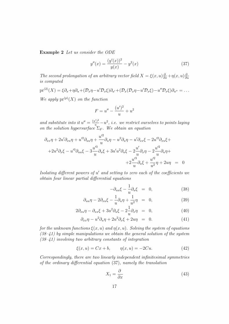
Example 2 Let us consider the ODE

y′′(x) =(y′(x))2

y(x)− y2(x) (37)

The second prolongation of an arbitrary vector field X = ξ(x, u) ∂∂x

+η(x, u) ∂∂u

is computed

pr(2)(X) = ξ∂x+η∂u+(Dxη−u′Dxξ)∂u′ +(Dx(Dxη−u′Dxξ)−u′′Dxξ)∂u′′ = . . .

We apply pr(p)(X) on the function

F = u′′ − (u′)2

u+ u2

and substitute into it u′′ = (u′)2

u−u2, i.e. we restrict ourselves to points laying

on the solution hypersurface ΣF . We obtain an equation

∂xxη + 2u′∂xuη + u′2∂uuη +u′2

u∂uη − u2∂uη − u′∂xxξ − 2u′2∂xuξ+

+2u2∂xξ − u′3∂uuξ − 3u′3

u∂uξ + 3u′u2∂uξ − 2

u′

u∂xη − 2

u′2

u∂uη+

+2u′3

u∂uξ +

u′2

u2η + 2uη = 0

Isolating different powers of u′ and setting to zero each of the coefficients weobtain four linear partial differential equations

−∂uuξ −1

u∂uξ = 0, (38)

∂uuη − 2∂xuξ −1

u∂uη +

1

u2η = 0, (39)

2∂xuη − ∂xxξ + 3u2∂uξ − 21

u∂xη = 0, (40)

∂xxη − u2∂uη + 2u2∂xξ + 2uη = 0. (41)

for the unknown functions ξ(x, u) and η(x, u). Solving the system of equations(38–41) by simple manipulations we obtain the general solution of the system(38–41) involving two arbitrary constants of integration

ξ(x, u) = Cx+ b, η(x, u) = −2Cu. (42)

Correspondingly, there are two linearly independent infinitesimal symmetriesof the ordinary differential equation (37), namely the translation

X1 =∂

∂x(43)

17

with the flow Φ1(x, u; t) = (x+ t, u), and a scaling symmetry

X2 = −x ∂∂x

+ 2u∂

∂u(44)

with the flow Φ2(x, u; t) = (e−tx, e2tu). The action of these point transfor-mations on functions y(x) is

(t .1 y)(x) = y(x− t)

and(t .2 y)(x) = e2ty(etx),

respectively.

In the case of PDEs the full derivation and intermediate calculations arevery long. Therefore, we shall only review and interpret the results.

Example 3 The heat equation

∂tu− ∂xxu = 0 (45)

has an infinite dimensional algebra of infinitesimal point symmetries. It con-sists of the six vector fields

X1 = 4xt∂x + 4t2∂t − (2t+ x2)u∂u,

X2 = 2x∂x + 4t∂t − u∂u,X3 = ∂t,

X4 = −2t∂x + xu∂u,

X5 = u∂u,

X6 = ∂x

together with an infinite set of generators

XV = V (x, t)∂u

where V (x, t) is an arbitrary solution of the heat equation (45).It is instructive to interpret these vector fields in terms of the correspond-

ing finite transformations. The vector fields X3, X6 generate translations int and x. These symmetries are obvious from the onset – they just representthe fact that the heat equation (45) is autonomous, i.e. does not involve tand x explicitly.

The vector fields X2, X5 represent invariance of the heat equation undertwo independent scalings u→ λu and x→ λx, t→ λ2t.

18

The vector field X4 indicates invariance under the Galilei transformationx→ x− λt accompanied by a suitable redefinition of u(x, t).

Finally, XV generates the invariance under the transformation u → u +λV where V is another arbitrary solution of the heat equation (45), i.e. rep-resents its linearity.

Altogether, all the symmetry generators X2, . . . , X6, XV can be guessedwithout any calculations. They close into a subalgebra of the full symmetryalgebra sym(∂tu − ∂xxu = 0) = span{X1, . . . , X6, XV }∂tV−∂xxV=0. Withoutexplicit computation of the symmetry algebra one would probably miss thegenerator X1 which does not possess any obvious physical interpretation.

As far as the algebraic structure of the Lie algebra sym(∂tu − ∂xxu = 0)is considered, we notice that it splits into a semidirect sum,

sym(∂tu− ∂xxu = 0) = span{XV }∂tV−∂xxV=0 +⊃ span{X1, . . . , X6}

where span{XV }∂tV−∂xxV=0 is an infinite–dimensional Abelian Lie algebraand span{X1, . . . , X6} is a finite dimensional Levi decomposable algebra. Ithas a simple factor span{X1, X2, X3} isomorphic to sl(2) and a nilpotentradical span{X4, X5, X6} isomorphic to the Heisenberg algebra h(1) whichis a nilpotent Lie algebras spanned by three vectors e1, e2, e3 with the onlynonvanishing Lie bracket

[e2, e3] = e1.

We observe that the infinite dimensional algebra span{XV }∂tV−∂xxV=0 is of-ten truncated to a finite dimensional subalgebra when the symmetries arecomputed using algorithms implemented in computer algebra systems (e.g.procedure Infinitesimals in Maple 13).

We have noticed in this example that often most, if not all, infinitesimalsymmetries of the given differential equation can be found by inspection,without any computation. Unfortunately, there is no easy way of establishingthe completeness of the symmetry algebra guessed in this way, e.g. there is nomethod of independent determination of dimension of the symmetry algebra.The only reliable method is to perform the full computation of symmetriesand check whether anything unexpected arises.

5 Applications: Reduction of the order of a

given ODE and others

Once the symmetry algebra of the given equation(s) is determined, one canuse it in several different ways such as:

19

1. Exponentiate infinitesimal symmetries to 1–parameter subgroups anduse the resulting transformations to generate new solutions from theknown ones.

2. Use the symmetry algebra as a necessary criterion for equivalence of twodifferential equations. If any pair of differential equations can be trans-formed one into the other by a point transformation then necessarilytheir symmetry algebras must be isomorphic. Thus we have a neces-sary (though far from sufficient) condition for equivalence. In addition,when an explicit transformation between two equations is sought, it isoften convenient to construct point transformations taking one sym-metry algebra into the other and only then look for transformationstaking one equation into the other inside this class.

In particular, when a given PDE has an infinite dimensional Abeliansubalgebra of infinitesimal symmetries involving an arbitrary solutionof some linear PDE we may interpret it as a strong indication that ourprescribed equation may be linearizable by some point transformation.

3. Reduce the order of an ODE. This method is based on a simple obser-vation that an ODE

F (x, y, . . . , y(p)) = 0

which possesses an infinitesimal symmetry ∂y must be independent ofthe dependent variable y, i.e. in the form

F (x, y′, . . . , y(p)) = 0 (46)

(possibly up to a multiplication by a common nonvanishing y–dependentprefactor which does not affect its solutions). Obviously, we may lowerits order by one through the substitution z = y′, then attempt to solvethe new ODE

F (x, z, . . . , z(p−1)) = 0

and once its solution z(x) is known, we may write the solution of theoriginal equation (46) in quadrature

y(x) =

∫z(x)dx.

Hence, the substance of the method is the following: starting from anarbitrary nonvanishing infinitesimal symmetry X = ξ∂x + η∂y we lookfor a point transformation, i.e. a change of coordinates on M × N ,such that in the new coordinates x, y our vector field X takes the form

20

X = ∂y. According to the rules for transformation of the componentsof a vector field these new coordinates must satisfy equations

X(x) = 0, X(y) = 1.

These equations are solved using the method of characteristics. Theirsolution is in general not unique, but any particular solution with non-constant x can be used.

Once x, y are found, we lower the order of our equation in the newcoordinates, solve it (if possible), and at the end transform the solutionto the original coordinates.

This approach generalizes many particular methods used in solution ofODEs.

Example 4 LetF (y, . . . , y(p)) = 0

be an autonomous ODE, i.e. not depending explicitly on x. It is in-variant under translations in the independent variable x, generated byX = ∂x. Therefore, if we interchange the roles of independent and de-pendent variable x = y, y = x, the vector field becomes X = ∂y and wemay lower the order of the differential equation for the inverse functionx(y) by one.

Example 5 LetF (x, y, . . . , y(p)) = 0 (47)

be invariant under the scaling x → λx, y → λαy. Such scaling isobtained as the 1–parameter group of transformations generated by thevector field

X = x∂x + αy∂y.

The new coordinates x, y can be chosen as

x =y

xα, y = lnx.

Once we rewrite the original ODE (47) in these coordinates we mayagain lower its order by one.

We remark that the reduced equation may have a group of symmetriesrather distinct from the original one. In particular, other symmetries

21

of the original equation may not survive the reduction. Only the sym-metries generated by such vector fields Y ∈ X(M ×N) that a constantα ∈ F exists satisfying

[Y,X] = αX

are guaranteed to survive the reduction.

By induction, a k–dimensional algebra of infinitesimal symmetries of agiven ODE with a complete flag of ideals as in Lie’s theorem4 allows usto reduce the order by k provided we can find suitable coordinates ineach step, of course. That was the original motivation for the definitionof a solvable algebra – although, as we have seen in Lie’s theorem, itis in the current terminology well justified only if we consider complexLie algebras and complex (holomorphic) ODEs.

Example 6 Let us use the symmetries computed in Example 2 to solvethe ordinary differential equation (37). Since we have [X1, X2] = −X1

we shall use the vector field X1 first. The suitable new coordinates inwhich we have X1 = ∂u are obviously

x = u, u = x,

i.e. we use a so–called hodograph transformation. The equation (37)when expressed in these new coordinates becomes

y′′(x) = − y′(x)

x+ x2(y′(x))3

and we can lower its degree using the substitution

z(x) = y′(x).

4

Theorem 4 (Theorem of Lie) Any representation ρ of a solvable Lie algebra g on acomplex finite–dimensional vector space V contains a common eigenvector v ∈ V, v 6= 0,i.e.

ρ(x)v = λ(x) · v, x ∈ g (48)

for some linear functional λ on g.For any complex solvable Lie algebra g there exists a filtration by codimension 1 ad–

invariant subspaces, i.e.

0 ( V1 ( V2 ( . . . ( Vdim g = g, dimVk/ dimVk−1 = 1, [g, Vk] ⊆ Vk. (49)

Lie’s theorem implies that any complex solvable Lie algebra g has only one–dimensionalirreducible representations and that the adjoint representation of any complex non–Abeliansolvable Lie algebra g is not fully reducible.

22

We obtain an equation

z′(x) = − z(x)

x+ x2(z(x))3 (50)

The vector field X2 in the new coordinates becomes

X2 = 2x∂

∂x− u ∂

∂u.

Its first prolongation is

pr(1)X2 = 2x∂

∂x− u ∂

∂u− 3z

∂

∂z.

We see that dropping the ∂∂u

term we obtain a well defined vector field

X2 = 2x∂

∂x− 3z

∂

∂z

on a two–dimensional space with coordinates x, z. The vector field X2

is by construction an infinitesimal symmetry of the equation (50). Now,we use it to further lower the order of the equation (50), i.e. to convertit into an algebraic equation. We find suitable new coordinates

x = x3z2, z = −1

2ln x

in which our equation (50) becomes

z′(x) = − 1

2(x+ 2x2). (51)

Integrating the equation (51) we find

z(x) =1

2ln

∣∣∣∣1 + 2x

x

∣∣∣∣− 1

2lnC

where C is a constant of integration. Going back to the coordinates x, zwe get an expression for the function z(x),

z(x) =1

x√C − 2x

.

Now we can further integrate

y(x) =

∫z(x)dx = − 2√

Carctanh

√C − 2x

C+D

23

where D is a second constant of integration. Finally, we transform thefunction y(x) to the original coordinates and find a general solution ofthe ODE (37) in the form

y(x) =C

2

(1− tanh2

(√C

2(D − x)

)). (52)

This reduction method can be immediately generalized to systems ofODEs but not to PDEs. For PDEs, another method is available.

4. Construction of group–invariant solutions of PDEs. As already men-tioned, the method described above does not work for PDEs since thefact that a PDE does not involve the dependent variable explicitly doesnot in general provide any help in its solution. Nevertheless, we mayemploy the symmetries in construction of particular solutions of a givenPDE.

The essential observation is as simple as above. Let us suppose that agiven PDE

F (xi, uα, . . . , uαJ) = 0

has a symmetry generatorX = ∂x1 . (53)

That means that F is invariant with respect to translations in x1, i.e.does not depend on it explicitly. Consequently, we may suppose thatour solution uα depends only on the remaining independent variablesxi, i = 2, . . . ,m and in this way we obtain a well–defined PDE with oneless independent variables. Any solution of this PDE is also a solutionof the original equation which in addition is invariant with respect tothe 1–parameter group of symmetries generated by the vector field X;hence its name group–invariant solution.

Similarly as before, the method boils down to the construction of suit-able coordinates xi, uα on M ×N in which a given symmetry generatorX takes the form (53). Again, the method of characteristics is used.In fact, it turns out that we need to compute only the invariant coor-dinates

xi : X(xi) = 0, i = 2, . . . ,m, uα : X(uα) = 0, α = 1, . . . , n

in the process, as the following example will demonstrate.

24

Example 7 Let us consider the heat equation of Example 3 and thevector field

X4 = −2t∂x + xu∂u.

This vector field has the following invariants

τ = t, I = uex2

4t .

Therefore, we substitute u(x, t) = I(t)e−x2

4t into the heat equation (45)and obtain a reduced equation for I(t)

2tI ′(t) + I(t) = 0.

Its general solution is I(t) = C√t. Altogether, we have recovered the

fundamental solution (when C = 1√4π

) of the heat equation

u(x, t) =C√te−

x2

4t

as the solution invariant with respect to Galilei transformations gener-ated by the vector field X4.

As before, the reduced equation may have symmetries which are of nodirect relation to the original ones. If we want to be able to further re-duce the number of independent variables we again need a solvable sym-metry algebra and an appropriate choice of generators of 1–parametersubgroups (i.e. a basis respecting the flag of codimension 1 ideals,starting from the smallest one).

We notice that solutions invariant with respect to vector fields X andX = AdgX are related: we may obtain a solution u(x) invariant withrespect to X from u(x) simply by setting u(x) = g . u(x). Therefore,one shall first classify 1–dimensional subalgebras of the symmetry alge-bra under conjugation by g ∈ G (or higher–dimensional subalgebras ifreduction with respect to more independent variables is intended) andonly then perform the reduction with respect to nonequivalent genera-tors.

25

Index

1–parameter subgroup, 71–parameter symmetry group, 11

action of Lie group, 5adjoint, 5effective, 5

contact transformation, 14

exponential map, 4

flow of vector field, 8

group of symmetries, 7group of transformations, 6group–invariant solution, 24

infinitesimal action, 6infinitesimal symmetry, 8infinitesimal transformation, 6

left–invariant vector field, 3Lie algebra, 4

structure constants, 4Lie algebra of Lie group, 4Lie group, 3

operator of total derivative, 12

point transformation, 10prolongation of vector field, 12prolonged graph, 10

representationof Lie group, 5

symmetry of algebraic equation, 7

theoremof Lie, 22on generators of symmetries, 9

on generators of symmetries of ODEs,13

on generators of symmetries of PDEs,15

26

References

[1] S. Lie, Theorie der Transformationsgruppen, Teil I–III. Leipzig: Teubner,1888, 1890, 1893.

[2] S. Lie, “Allgemeine Untersuchungen uber Differentialgleichungen, die einecontinuirliche, endliche Gruppe gestatten,” Math. Ann., vol. 25, no. 1,pp. 71–151, 1885.

[3] S. Lie, “Classification und Integration von gewohnlichen Differentialgle-ichungen zwischen xy, die eine Gruppe von Transformationen gestatten,”Math. Ann., vol. 32, no. 2, pp. 213–281, 1888.

[4] S. Lie, Vorlesungen uber continuierliche Gruppen mit Geometrischen undanderen Anwendungen. Leipzig: Teubner, 1893.

[5] P. J. Olver, Applications of Lie groups to differential equations, vol. 107of Graduate Texts in Mathematics. New York: Springer-Verlag, 1986.

[6] P. E. Hydon, Symmetry methods for differential equations: A beginner’sguide. Cambridge Texts in Applied Mathematics, Cambridge: CambridgeUniversity Press, 2000.

27