Part A1: Differential Equations I

Lecture notes by Janet Dyson *

MT 2020Lecturer: Melanie Rupflin

Contents

1 ODEs and Picard’s Theorem 4

1.1 Introduction . . . . . . . . . . . . . . . . . . . . . . . . . . . . . . . . . . . 4

1.2 Picard’s method of successive approximation . . . . . . . . . . . . . . . . 6

1.3 Picard’s Theorem . . . . . . . . . . . . . . . . . . . . . . . . . . . . . . . . 8

1.4 Extension of solutions and global existence. . . . . . . . . . . . . . . . . . 12

1.5 Gronwall’s inequality and continuous dependence on the initial data. . . . 14

1.6 Picard’s Theorem via the CMT . . . . . . . . . . . . . . . . . . . . . . . . 15

1.7 Picard’s Theorem for systems and higher order ODEs via the CMT . . . . 20

1.8 Summary . . . . . . . . . . . . . . . . . . . . . . . . . . . . . . . . . . . . 23

2 Plane autonomous systems of ODEs 24

2.1 Critical points and closed trajectories . . . . . . . . . . . . . . . . . . . . 24

2.1.1 An example . . . . . . . . . . . . . . . . . . . . . . . . . . . . . . . 25

2.2 Stability and linearisation . . . . . . . . . . . . . . . . . . . . . . . . . . . 26

2.3 Classification of critical points . . . . . . . . . . . . . . . . . . . . . . . . . 28

2.3.1 An example . . . . . . . . . . . . . . . . . . . . . . . . . . . . . . . 34

2.3.2 Further example: the damped pendulum . . . . . . . . . . . . . . . 36

2.3.3 An important example: The Lotka–Volterra predator-prey equations 37

*based on notes by Peter Grindrod, Colin Please, Paul Tod, Lionel Mason and others, with modifi-cations in chapter 1 by the lecturer

1

2.3.4 Another example from population dynamics. . . . . . . . . . . . . 38

2.3.5 Another important example: limit cycles . . . . . . . . . . . . . . . 39

2.4 The Bendixson–Dulac Theorem . . . . . . . . . . . . . . . . . . . . . . . . 43

2.4.1 Corollary. . . . . . . . . . . . . . . . . . . . . . . . . . . . . . . . . 43

2.4.2 Examples . . . . . . . . . . . . . . . . . . . . . . . . . . . . . . . . 43

3 First order semi-linear PDEs: the method of characteristics 45

3.1 The problem . . . . . . . . . . . . . . . . . . . . . . . . . . . . . . . . . . 45

3.2 The big idea: characteristics . . . . . . . . . . . . . . . . . . . . . . . . . . 46

3.2.1 Examples of characteristics . . . . . . . . . . . . . . . . . . . . . . 47

3.3 The Cauchy problem . . . . . . . . . . . . . . . . . . . . . . . . . . . . . . 48

3.4 Examples . . . . . . . . . . . . . . . . . . . . . . . . . . . . . . . . . . . . 49

3.5 Domain of definition . . . . . . . . . . . . . . . . . . . . . . . . . . . . . . 51

3.6 Cauchy data and the Cauchy Problem: . . . . . . . . . . . . . . . . . . . 55

3.7 Discontinuities in the first derivatives . . . . . . . . . . . . . . . . . . . . . 55

3.8 General Solution . . . . . . . . . . . . . . . . . . . . . . . . . . . . . . . . 57

4 Second order semi-linear PDEs 58

4.1 Classification . . . . . . . . . . . . . . . . . . . . . . . . . . . . . . . . . . 58

4.1.1 The idea: . . . . . . . . . . . . . . . . . . . . . . . . . . . . . . . . 58

4.1.2 The Classification . . . . . . . . . . . . . . . . . . . . . . . . . . . 59

4.2 Characteristics: . . . . . . . . . . . . . . . . . . . . . . . . . . . . . . . . . 65

4.3 Type and data: well posed problems . . . . . . . . . . . . . . . . . . . . . 66

4.4 The Maximum Principle . . . . . . . . . . . . . . . . . . . . . . . . . . . . 72

4.4.1 Poisson’s equation . . . . . . . . . . . . . . . . . . . . . . . . . . . 72

4.4.2 The heat equation . . . . . . . . . . . . . . . . . . . . . . . . . . . 76

5 Where does this course lead? 79

5.1 Section 1 . . . . . . . . . . . . . . . . . . . . . . . . . . . . . . . . . . . . 79

5.2 Section 2 . . . . . . . . . . . . . . . . . . . . . . . . . . . . . . . . . . . . 79

5.3 Section 3 . . . . . . . . . . . . . . . . . . . . . . . . . . . . . . . . . . . . 80

5.4 Section 4 . . . . . . . . . . . . . . . . . . . . . . . . . . . . . . . . . . . . 80

2

Introduction

The solution of problems in most parts of applied mathematics and many areas of purecan more often than not be reduced to the problem of solving some differential equa-tions. Indeed, many parts of pure maths were originally motivated by issues arising fromdifferential equations, including large parts of algebra and much of analysis, and Differ-ential equations are a central topic in research in both pure and applied mathematics tothis day. From Prelims, and even from school, you know how to solve some differentialequations. Indeed most of the study of differential equations in the first year consistedof finding explicit solutions of particular ODEs or PDEs. However, for many differentialequations which arise in practice one is unable to give explicit solutions and, for themost part, this course will consider what information one can discover about solutionswithout actually finding the solution. Does a solution exist? Is it unique? Does itdepend continuously on the initial data? How does it behave asymptotically? What isappropriate data?

So, first we will develop techniques for proving Picard’s theorem for the existence anduniqueness of solutions of ODEs; then we will look at how phase plane analysis enablesus to estimate the long term behaviour of solutions of plane autonomous systems ofODEs. We will then turn to PDEs and show how the method of characteristics reducesthe solution of a first order semi-linear PDE to solving a system of non-linear ODEs.Finally we will look at second order semi-linear PDEs: We classify them and investigatehow the different types of problem require different types of boundary data if the prob-lem is to be well posed. We then look at how the maximum principle enables us to proveuniqueness and continuous dependence on the initial data for two very special problems:Poisson’s equation and the inhomogeneous heat equation – each with suitable data.

Throughout, we shall use the following convenient abbreviations: we shall write

DEs: for differential equations.

ODEs: for ordinary DEs, i.e. differential equations with only ordinary derivatives.

PDEs: for partial DEs, i.e. differential equations with partial derivatives.

The course contains four topics, with a section devoted to each. The chapters are:

1. ODEs and Picard’s Theorem (for existence/uniqueness of solutions/continuous de-pendence on initial data).

2. Plane autonomous systems of ODEs

3. First order semi-linear PDEs: the method of characteristics.

4. Second-order semi-linear PDEs: classification; well posedness; the Maximum Prin-ciple and its consequences

3

Books

The main text is P J Collins Differential and Integral Equations, O.U.P. (2006), whichcan be used for the whole course (Chapters 1-7, 14, 15).

Other good books which cover parts of the course include

W E Boyce and R C DiPrima, Elementary Differential Equations and Boundary ValueProblems, 7th edition, Wiley (2000).

E Kreyszig, Advanced Engineering Mathematics, 8th Edition, Wiley (1999).

G F Carrier and C E Pearson, Partial Differential Equations – Theory and Technique,Academic (1988).

J Ockendon, S Howison, A Lacey and A Movchan, Applied Partial Differential Equations,Oxford (1999) [a more advanced text].

4

PART I Ordinary Differential Equations

1 ODEs and Picard’s Theorem

1.1 Introduction

An ODE is an equation for y(x) of the form

G(x, y, y′, y′′, ..., y(n)) = 0.

We refer to y as the dependent variable and x as the independent variable. Usually thiscan be solved for the highest derivative of y and written in the form

dny

dxn:= y(n)(x) = F (x, y, y′, ..., y(n−1)).

Then the order of the ODE is n, the order of the highest derivative which appears.Given an ODE, certain obvious questions arise. We could ask:

• Does it have solutions? Can we find them (explicitly or implicitly)? If not, can weat least say something about their qualitative behaviour?

• Given data e.g. the values y(a), y′(a), ... of y(x) and its first n − 1 derivativesat some initial value a of x, does it have a solution? is it unique? does it dependcontinuously on the given data?

We shall consider these questions in Part I.

For simplicity, we begin with a first-order ODE with data:

y′(x) = f(x, y(x)) with y(a) = b. (1.1)

This is an initial value problem or IVP, since we are given y at an initial, or starting,value of x. You know how to solve a variety of equations like this. You might expect thata solution exists, so there is some function that satisfies the equations (even if you cannotfind a formula for it) and perhaps you expect, for a given initial values, the solution isunique (there is only one function that satisfies the ODE and the initial data) as youmay not have encountered the following difficulties.

Warning examples:

Consider this IVP:y′ = 3y2/3; y(0) = 0. (1.2)

5

So separate the variables (a prelims technique):∫dy

3y2/3=

∫dx,

to get y = (x+A)3, so if y(0) = 0

(i) There is a solution y = x3;

(ii) But evidently there is another solution: by direct checking y = 0 will do;

(iii) In fact we can find that there are infinitely many solutions. Pick a, b with a ≤ 0 ≤ band define

y = (x− a)3 x < a

= 0 a ≤ x < b

= (x− b)3 b ≤ x

The solution does exist but is not unique (in fact far from it, since we’ve found infinitelymany solutions).

Furthermore, even if a solution of (1.1) exists, it may not exist for all x.

For example consider the IVP

y′ = y2; y(0) = 1. (1.3)

Using separation of variables we can see this has solution y =1

1− x; so y → ∞ as

x → 1, and the solution only exists on x < 1. We will see later that this solution is infact unique.

So, if we want to have a unique solution to the problem (1.1) we must impose conditionson f , and we cannot necessarily expect to have solutions for all x. This will be the firstexistence theorem which you’ve encountered. The proof is quite technical, certainly themost technical thing in the course. In particular, you need to remember from Prelimsthe Weierstrass M-test for convergence of a series of functions.

To be precise then, we shall seek a solution of problem (1.1) in a rectangle R about theinitial point (x, y) = (a, b), so suppose R = {(x, y) : |x− a| ≤ h, |y− b| ≤ k} as in figure1.1:

6

2h

2k

a

bR

y

x

Figure 1.1: The rectangle R

Our first assumption is that f : R → R is continuous in R. Note that if y is asolution of (1.1), say on an interval [a−h, a+h], then integrating (1.1) from a to variablex ∈ [a− h, a+ h] yields

y(x)− y(a) = [y(t)]xa =

∫ x

af(t, y(t))dt

for any x so rearranging

y(x) = b+

∫ x

af(t, y(t))dt. (1.4)

We note that since f : R→ R and y : [a−h, a+h]→ R are continuous, also the functionx 7→ f(x, y(x)) is continuous function on [a− h, a+ h] so integrable.

Conversely, if y(t) is continuous on [a − h, a + h] and satisfies (1.4), then y(a) = band by the Fundamental theorem of Calculus we can differentiate (1.4) to get that yis a solution of (1.1). Thus (1.1) and (1.4) are equivalent. We have transformed thedifferential equation to an integral equation - the unknown y is given in terms of anintegral rather than a differential. There is a general theory of these, but we only needto deal with the particular case of (1.4). The standard approach is to seek a solution byiteration or successive approximation.

1.2 Picard’s method of successive approximation

We start with an initial guess and then improve it. The guesses, or successive approxi-mations or iterates, are labeled yn(x) starting with y0(x). Take

y0(x) = byn+1(x) = b+

∫ xa f(t, yn(t))dt

}(1.5)

That is, we start with the simplest guess, that y equals its initial value, and at each stagesubstitute the current guess into the right-hand-side of (1.4) to get the next guess. We

7

need to know if this process converges, and if it does whether it converges to a solutionof the problem (1.4). Consider the differences between successive approximations:

e0(x) = ben+1(x) = yn+1(x)− yn(x)

}(1.6)

and note that

yn(x) =

n∑0

ek(x). (1.7)

We want yn to converge, so we want the series∑n

0 ek(x) to converge. So we mustestimate the differences en(x). This will need a condition on f , but here is the key idea.

Notice that

en+1(x) = yn+1(x)− yn(x) =

∫ x

a[f(t, yn(t))− f(t, yn−1(t))]dt

and recall that the modulus of the integral of a function is less than or equal to theintegral of the modulus (because the function can be negative). Therefore

| en+1(x)| ≤∣∣∣∣∫ x

a|f(t, yn(t))− f(t, yn−1(t))| dt

∣∣∣∣ . (1.8)

(The modulus outside the integral on the right hand side is required to cover the casex ≤ a.) We want to bound the integrand on the right-hand side in terms of the erroren(t) = |yn(t)− yn−1(t)| of the previous step which motivates the following definition:

Definition 1.1. A function f(x, y) on a rectangle R satisfies a Lipschitz condition (withconstant L) if ∃ real positive L such that

|f(x, u)− f(x, v)| ≤ L|u− v| for all (x, u) ∈ R, (x, v) ∈ R. (1.9)

This is a new condition on a function, stronger than being continuous in the secondvariable but weaker than being differentiable. It turns out to be the right condition tomake Picard’s theorem, which is the existence theorem we want, work, as it allows us tobound the integrand in (1.8) by

|f(t, yn(t))− f(t, yn−1(t))| ≤ L|en(t)|.

Important note: One way to ensure that f satisfies a Lipschitz condition on R is thefollowing: Suppose that, on R, f is differentiable with respect to y , with |fy(x, y)| ≤ K.Then for any (x, u) ∈ R, (x, v) ∈ R the mean value theorem (applied to the function[k − h, k + h] 3 y 7→ f(x, y)) gives

|f(x, u)− f(x, v)| = |fy(x,w)(u− v)| ≤ K|u− v| (1.10)

where w is some intermediate value. So, f clearly satisfies the Lipschitz condition onsuch intervals.

On the other hand f(y) = |y| is Lipschitz continuous, but is not differentiable at y = 0.

8

1.3 Picard’s Theorem

Theorem 1.1. (Picard’s existence theorem):

Let f : R→ R be a function defined on the rectangle R := {(x, y) : |x−a| ≤ h, |y−b| ≤ k}which satisfiesP(i): (a) f is continuous in R, with bound M (so |f(x, y)| ≤M) and (b) Mh ≤ k.P(ii): f satisfies a Lipschitz condition in R.

Then the IVPy′(x) = f(x, y(x)) with y(a) = b.

has a unique solution y : [a− h, a+ h]→ [b− k, b+ k].

We will prove the existence of a solution by showing that the iterates yn defined in (1.5)converge as n→∞ to a solution y of the IVP and will do this by showing that the seriesin (1.7) converges. We break the proof into a series of steps:

Claim 1: Each yn is well defined, continuous and |yn(x)− b| ≤ k for x ∈ [a− h, a+ h].

Proof of Claim 1: This is clearly true for n = 0, so suppose claim is true for somen ≥ 0. Then t ∈ [a−h, a+h] we have that (t, yn(t)) ∈ R so as f is defined and continuouson R and as yn is continuous we have that t 7→ f(t, yn(t)) is a continuous function onthe interval [a − h, a + h]. Thus yn+1 is well defined and continuous by properties ofintegration and by P(i)

|yn+1(x)− b| ≤∣∣∣∣∫ x

a|f(t, yn(t))|dt

∣∣∣∣≤

∣∣∣∣M ∫ x

adt

∣∣∣∣ = M |x− a| ≤Mh ≤ k

for every x ∈ [a− h, a+ h]. Thus the claim is true by induction.

Figure 1.2: successive iterates graphed in R.

We next prove:

9

Claim 2: For |x− a| ≤ h and n ∈ N

|en(x)| ≤ Ln−1M

n!|x− a|n (1.11)

where L is such that the Lipschitz condition (1.9) holds.

We remark that this claim in particualar implies that

|en(x)| ≤ Ln−1M

n!hn for all |x− a| ≤ h. (1.12)

which will be the estimate that we will use to show that∑en converges uniformly using

M-test.

Proof of Claim 2: We recall that the Lipschitz condition P(ii) combined with the factthat the graph of yn is in the rectangle implies that for all |t− a| ≤ h

|f(t, yn(t))− f(t, yn−1(t))| ≤ L|yn(t)− yn−1(t)| = L|en(t)|. (1.13)

From (1.8) and (1.13) thus

| en+1(x)| ≤∣∣∣∣∫ x

a|f(t, yn(t))− f(t, yn−1(t))|dt

∣∣∣∣≤ L

∣∣∣∣∫ x

a|en(t)|dt

∣∣∣∣ . (1.14)

Now we prove (1.11) by induction:

e1(x) = y1(x)− b =

∫ x

af(t, b)dt. (1.15)

By P(i), f is bounded by M so that

|e1(x)| ≤∣∣∣∣∫ x

a|f(t, b)|dt

∣∣∣∣ ≤M |x− a|, (1.16)

so (1.11) is true for n = 1. Now suppose that (1.11) is true for n, then

| en+1(x)| ≤ L

∣∣∣∣∫ x

a|en(t)|dt

∣∣∣∣≤ L

∣∣∣∣∫ x

a

Ln−1M

n!|t− a|ndt

∣∣∣∣ =LnM

(n+ 1)!|x− a|n+1,

so that (1.11) is true by induction.

We now use these two claims to prove the existence of a solution to the integral equation(1.4) by showing

10

Claim 3: The iterates yn(x) =∑n

j=0 ej(x) converge uniformly to a continuous functiony∞ and y∞ is a solution of the integral equation (1.4).

Proof of Claim 3: The uniform convergence immediately follows from the Weierstrass

M -test and (1.12), since∑∞

n=1Mn for Mn =Ln−1Mhn

n!converges and Mn is a upper

bound on |en(x)| that is independent of x. Thus, yn =∑n

0 ek converges uniformly to alimit y∞ on [a − h, a + h] and this limit is continuous as it is the uniform limit of thecontinuous functions yn.

To see that y∞ is a solution of (1.1), we would like to take the limit in (1.5) and exchangethe limit and the integral to get that

y∞(x) = limn→∞

yn+1(x) = b+ limn→∞

∫ x

af(t, yn(t))dt

(∗)= b+

∫ x

alimn→∞

f(t, yn(t))dt

= b+

∫ x

af(t, y∞(t))dt.

(1.17)

The reason that we are allowed to switch limit and integral in (*) is that the integrandsf(t, yn(t)) converge uniformly to f(t, y∞(t)) since the uniform convergence of the yn andthe Lipschitz condition allow us to estimate

supt∈[a−h,a+h]

|f(t, yn(t))− f(t, y∞(t))| ≤ supt∈[a−h,a+h]

L|yn(t)− y∞(t)| → 0.

We have thus proven the existence of a solution of the integral equation and as remarkedpreviously differentiating the integral equation implies that

y′∞(x) = f(x, y∞(x))

and since also y∞(a) = b, thus y∞ is a solution of the IVP.

This completes the proof of existence and it remains to show

Claim 4: The solution of (1.1) is unique among all functions y : [a − h, a + h] →[b− k, b+ k].

Proof of Claim 4: Let y1(x) and y2(x) be two solutions of (1.1) (for the same f , aand b!) and set e(x) := y2(x)− y1(x). We aim to show that e(x) = 0 for all x.

As the IVP is equivalent to the integral equation (1.4) we can subtract the two integralequations satisfied by y1,2 to see that

e(x) = y2(x)− y1(x) =

∫ x

a(f(t, y2(t))− f(t, y1(t)))dt

so using the triangle inequality for integrals and the Lipschitz condition we get

| e(x)| ≤∣∣∣∣∫ x

a|f(t, y2(t))− f(t, y1(t))|dt

∣∣∣∣ ≤ L ∣∣∣∣∫ x

a|y2(t)− y1(t)|dt

∣∣∣∣≤ L

∣∣∣∣∫ x

a|e(t)|dt

∣∣∣∣ (1.18)

11

Now e(x) is continuous on [a− h, a+ h] therefore, it is bounded say |e(x)| ≤ B so

| e(x)| ≤ L∣∣∣∣∫ x

aBdt

∣∣∣∣ = LB|x− a|

and inducting on n, using (1.18), for each n

| e(x)| ≤ BLn |x− a|n

n!

So that for each n

| e(x)| ≤ BLnhn

n!→ 0 as n→∞ and e(x) = 0.

Thus the difference is zero, so the solutions are the same which establishes uniqueness(uniqueness proofs almost always go like this: assume there are two and make theirdifference vanish).

This completes the proof of Picard’s Theorem.

Since the warning example doesn’t have a unique solution, something goes wrong forit. As an exercise, show that the warning example fails the Lipschitz condition (in anyneighbourhood of the initial point).

The following example also fails the Lipschitz condition in any neighbourhood of theinitial point y = 0. However, the Lipschitz condition does hold on any rectangle whichdoes not contain any point (x, 0).

Example: Consider the IVP

y′ = x2y1/5, y(0) = b.

So we consider the function f : R2 → R defined by f(x, y) = x2y1/5 which is clearlycontinuous. (Note that when we write y1/5 here we mean to take the real root: so thatif y is negative we will take −|y|1/5.)

Case b = 0: f(x, y) does not satisfy a Lipschitz condition on any rectangle of the formR0 = {(x, y) : |x| ≤ h, |y| ≤ k}, where h > 0 and k > 0.

Suppose it does, then there exists a finite constant L such that for all |x| ≤ h and|y|, |y| ≤ k

|x2||y1/5 − y1/5| ≤ L|y − y|

so in particular (choosing y = 0 and x = h)

|h2||y−4/5| ≤ L for every y ∈ [−h, h] \ {0}.

But this is a contradiction as |h2||y−4/5| is unbounded as y → 0 so the function does notsatisfy a Lipschitz condition on R0. So Picard’s theorem does not apply if we take b = 0.(We saw that f satisfies a Lipschitz condition on any rectangle where its derivative with

12

respect to y exists and is bounded. The problem here is that the derivative of f isunbounded as y → 0 – indeed the derivative does not exist at y = 0.)

Case b > 0: However, the assumptions of Picard’s theorem will be satisfied if we take asinitial condition y(0) = b > 0, provided we take a rectangle, Rb, given by Rb = {|x| ≤ h,|y − b| ≤ k} when 0 < k < b, so that y cannot be zero in this rectangle .

On any such rectangle fy(x, y) = x2y−4/5

5 is bounded, so, by (1.10), f satisfies a Lipschitzcondition, and P(ii) is satisfied.

For P(i): f(x, y) is continuous on Rb and

maxRb|x2y1/5| ≤ h2(b+ k)1/5 =: M,

so Picard’s theorem applies in a rectangle where h > 0 satisfies

h2(b+ k)1/5h ≤ k.

That is

h3 ≤ k

(b+ k)1/5. (1.19)

We can of course solve this problem directly using separation of variables if we wishgiving

y =(

4x3/15 + b4/5)5/4

,

so actually the solution exists for all x. Note the solution above is valid for b = 0 BUTthe trivial solution is also valid. So while we still have existence, uniqueness does nothold.

Remark: Note that the proof of uniqueness of the solution only holds among thosesolutions whose graph lies in R. However, actually, if P(i) and P(ii) hold, then, for|x− a| ≤ h, the graph of any solution of (1.1) must lie in R.

Indeed, suppose not. Then, by the continuity of y, there will exist a ‘first’ x0, with|x0 − a| < h, where (x0, y(x0)) is on the boundary of R. That is such that |x0 − a| < h,|y(x0)− b| = k but |y(x)− b| < k if |x− a| < |x0 − a|, see figure 1.3. But then

|y(x0)− b| ≤∣∣∣∣∫ x0

a|f(s, y(s))|ds

∣∣∣∣ ≤M |x0 − a| < Mh = k

a contradiction.

1.4 Extension of solutions and global existence.

The result in Section 1.5 is a local result in that it guarantees existence and uniquenessof a solution on the interval [a−h, a+h], where h satisfies Mh ≤ k (though this h neednot be the best possible).

13

Figure 1.3:

As we have seen there are examples of initial value problems where solutions do notexist for all x ∈ (−∞,∞). So we would like to find conditions which guarantee that thesolution does exist for all x ∈ (−∞,∞) (or if f is only defined for x in an certain intervalthen on the whole such interval). One such condition is the global Lipschitz condition,where we can find a constant L such that the Lipschitz condition holds for all y. First wewill see that if the Lipschitz condition is global in y, but L still depends on the interval[a− h, a+ h], then there is existence on all of [a− h, a+ h]

Suppose we require that f(x, y) is defined and continuous for all (x, y) ∈ [a−h, a+h]×Rand instead of (P(ii)) we have

(P(iii)): f(x, y) satisfies the Lipschitz condition for all real y and all x ∈ [a− h, a+ h].

Then the last condition in claim 1 is not required and hence we don’t need to askthat Mh ≤ k. If we investigate the proof of the Picard existence theorem, we seethat M also appears in (1.16). However for claim 2 to hold it is sufficient to takeM = supx∈[a−h,a+h] |f(x, b)|, which exists as x 7→ f(x, b) is a continuous function on theclosed bounded interval [a− h, a+ h] (whereas (x, y) 7→ f(x, y) might be unbounded onthe unbounded set [a−h, a+h]×R) . The rest of the proof applies without change andwe hence obtain that the solution exists and is unique ∀x ∈ [a− h, a+ h].

14

Iif (P(iii)) holds for each h > 0 (for some L that is allowed to depend on h), then wecan carry out this argument for every h > 0 and, by letting h → ∞ deduce that thesolution exists on all of R. In this case we say that we have a global solution.

Example: If f(x, y) = p(x)y + q(x), where p and q are continuous on |x− a| ≤ h, thenf satisfies (P(iii)).

Remark We do not need the interval in (P(iii)) to be a balanced interval (ie of the form[a−h, a+h]) because we can deal with x ≤ a and x ≥ a separately. Thus if a ∈ [c, d] andwe require that f is continuous on [c, d]×R and that it satisfies the Lipschitz conditionon this set, then a solution of (1.1) exists and is unique for all x ∈ [c, d].

1.5 Gronwall’s inequality and continuous dependence on the initialdata.

We will now prove Gronwall’s inequality which will be used to provide another proof ofuniqueness of solutions, but will also be used to show that solutions depend continuouslyon the initial data.

Theorem 1.2. (Gronwall’s inequality) : Suppose A ≥ 0 and b ≥ 0 are constantsand v is a non-negative continuous function satisfying

v(x) ≤ b+A

∣∣∣∣∫ x

av(s)ds

∣∣∣∣ (1.20)

thenv(x) ≤ beA|x−a|.

(The modulus is needed to take care of the case x ≤ a.)

Proof: We use an integrating factor.

For x ≥ a let V (x) =∫ xa v(s)ds, so that V ′(x) = v(x). As x ≥ z and v ≥ 0 also X(x) ≥ 0

and we haveV ′(x) ≤ b+AV (x).

Multiply through by the integrating factor e−Ax so

(V ′(x)−AV (x))e−Ax ≤ be−Ax that is

d

dx(V (x)e−Ax) ≤ be−Ax, so, integrating and noting that V (a) = 0

V (x)e−Ax ≤∫ x

abe−Asds =

b

A(e−Aa − e−Ax), so

V (x) ≤ b

A(eA(x−a) − 1).

Finally, using (1.20)

v(x) ≤ b+A

∫ x

av(s)ds = b+AV (x) ≤ b+A

b

A(eA(x−a) − 1) = beA(x−a),

15

as required. Similarly if x ≤ a.

Remark: Gronwall’s inequality says that v is bounded above by the solution of theintegral equation one obtains when there is equality in (1.20). For, if we differentiate

v(x) = b+A

∫ x

av(s)ds,

we getv′(x) = Av(x), v(a) = b,

which has solution v(x) = beA(x−a).

Suppose now that y and z are solutions of the ordinary differential equation y′(x) =f(x, y(x)) with y(a) = b and z(a) = c, where f satisfies conditions (P(i)) and (P(ii)).Then

y(x)− z(x) = b− c+

∫ x

a(f(s, y(s))− f(s, z(s))ds

so setting v(x) = |y(x)− z(s)| (note Gronvall requires v to be non-negative) we get that

|y(x)− z(x)| ≤ |b− c|+∣∣∣∣∫ x

aL|y(s)− z(s)|ds

∣∣∣∣and by Gronwall’s inequality

|y(x)− z(x)| ≤ |b− c|eL|x−a| ≤ |b− c|eLh. (1.21)

Thus we have related |y(x)− z(x)| to |b− c|.

We say a solution is continuously dependent on the initial data if we can make |y(x)−z(x)|as small as we like by taking |b−c| small enough. In other words the error in the solutionwill be small provided the error in the initial data is small enough. To be precise, in thiscase, solutions are continuously dependent on the initial data for x ∈ [a− h, a+ h] if forall ε > 0 there exists δ > 0 such that if y and z are as above,

|b− c| < δ ⇒ |y(x)− z(x)| ≤ ε, ∀x ∈ [a− h, a+ h].

This is clearly true from (1.21), because given ε > 0, we have |y(x)− z(x)| ≤ ε whenever|b− c| < e−Lhε, so we can take δ = e−Lhε.

We could also use this to prove uniqueness. If y and z are solutions with b = c, then weget y(x) = z(x) for every x so that solution is unique.

1.6 Picard’s Theorem via the CMT

We can prove Picard’s theorem in a more efficient way, which is really equivalent toour previous method, by using the contraction mapping theorem (CMT). This is a veryuseful method of proving existence and uniqueness of solutions of nonlinear differential

16

equations and many, many other things besides. The results we need will be discussed inthe course on Metric Spaces and Complex Analysis. We will assume the results provedthere.

Define Ch,k = C([a − h, a + h]; [b − k, b + k]), the space of continuous functions y :[a− h, a+ h]→ [b− k, b+ k]. As is shown in the Metric Spaces course, for y, z ∈ Ch,k ifwe define

d(y, z) := ||y − z||sup := supx∈[a−h,a+h]

|y(x)− z(x)|

then (Ch,k, d) is a complete metric space (we call || · ||sup the “sup norm”).

Also we say that a map T : Ch,k → Ch,k is a contraction if there exists K < 1 such that

||T (y)− T (z)||sup ≤ K||y − z||sup,

and then we have the CMT, which says:

Theorem 1.3. (Contraction Mapping Theorem) (Banach) Let X be a completemetric space and let T : X → X be a contraction. Then there is a unique fixed pointy ∈ X, i.e. a unique y such that Ty = y.

To prove Picard’s Theorem via the CMT we will first apply this theorem for X = Cη,k =C([a− η, a+ η]; [b− k, b+ k]) for a small enough 0 < η ≤ h that we chose below, whichwill give that there exists a unique solution for |x−a| ≤ η. In a second step we will thendiscuss how this solution can be extended to all of [a− h, a+ h] if Mh ≤ k by repeatingthe argument with a new choice of the space X.

We again consider the IVP (1.1)

Theorem 1.4. (Picard’s existence theorem.) Let f : R → R be a function definedon the rectangle R := {(x, y) : |x−a| ≤ h, |y− b| ≤ k} which satisfies conditions P(i)(a)and P(ii) and let η > 0 be so that Lη < 1 and Mη ≤ k.

Then the initial value problem (1.1) has a unique solution for x ∈ [a− η, a+ η].

Proof.

The strategy is to express (1.1) as a fixed point problem and use the CMT.

As before, we can write the initial value problem as an integral equation

y(x) = b+

∫ x

af(s, y(s))ds (1.22)

Provided f(s, y(s)) is continuous in s, y is a solution of the differential equation if andonly if y is a solution of the integral equation.

If we define

(Ty)(x) = b+

∫ x

af(s, y(s))ds

17

then we can write (1.22) as a fixed point problem

y = Ty.

We will work in the complete metric space Cη,k = C([a − η, a + η]; [b − k, b + k]), wherewe will choose η ≤ h so that T : Cη,k → Cη,k and is a contraction. We begin by provingClaim 1: If η > 0 is so that Mη ≤ k then T : Cη,k → Cη,k

Proof. First we note that from the properties of integration, (Ty)(x) ∈ C([a−η, a+η];R).All that we require is thus to show that ||Ty − b||sup ≤ k if ||y − b||sup ≤ k.

But

||Ty − b||sup = supx∈[a−η,a+η]

∣∣∣∣∫ x

af(s, y(s))ds

∣∣∣∣ (1.23)

≤ supx∈[a−η,a+η]

∣∣∣∣∫ x

a|f(s, y(s))|ds

∣∣∣∣ (1.24)

≤ Mη ≤ k, (1.25)

provided Mη ≤ k.

Claim 2: If Lη < 1 then T is a contraction (with K = Lη):

Proof. Given y, z ∈ Cη,k we can bound

||Ty − Tz||sup = supx∈[a−η,a+η]

∣∣∣∣∫ x

af(s, y(s))− f(s, z(s))ds

∣∣∣∣≤ sup

x∈[a−η,a+η]

∣∣∣∣∫ x

a|f(s, y(s))− f(s, z(s))|ds

∣∣∣∣≤ sup

x∈[a−η,a+η]

∣∣∣∣∫ x

aL|y(s)− z(s)|ds

∣∣∣∣ ≤ Lη||y − z||sup ≤ K||y − z||sup

where K := ηL < 1 provided η < 1/L.

If we hence choose η < min{h, k/M, 1/L} then T satisfies the conditions of the CMTand has a unique fixed point, y(x). As explained before, a (continuous) function y solvesthe integral equation Ty = y if and only if it is continuously differentiable and a solutionof the initial value problem, so we have established that the initial value problem has aunique solution on the interval [a− η, a+ η].

Note that our proof using CMT produces a more restricted range of x values than didour proof on one dimension. The range of η depends on L as well as M and k. However,if Mh ≤ k, actually we only need η ≤ h, and we can now extend the range of the solutionto all x ∈ [a− h, a+ h], by iteration.

18

Corollary 1.5. If Mh ≤ k, then the initial value problem has a unique solution on thewhole interval [a− h, a+ h]

Proof: We look at x ≥ a first. If h < 1/L we are done. (Take η = h.)

Otherwise we choose η1 < 1/L. Then, from Theorem 1.4, there exists a unique solution,y0 say, on [a, a+ η1] .

Now choose η2 = min{2η1, h}, and look for a solution, y1 say, on [a+ η1, a+ η2], of theODE with initial data y1(a+ η1) = y0(a+ η1).

Now definey(x) = y0(x), x ∈ [a, a+ η1]y(x) = y1(x), x ∈ [a+ η1, a+ η2]

To constuct y1: As in Theorem 1.4, but we now work in the space X1 := C([a+ η1, a+η2]; [b− k, b+ k]), and take (for a+ η1 ≤ x ≤ a+ η2)

(T1y)(x) = y0(a+ η1) +

∫ x

a+η1

f(s, y(s))ds

= b+

∫ a+η1

af(s, y0(s))ds+

∫ x

a+η1

f(s, y(s))ds. (1.26)

So T1 : X1 → X1 because from (1.26)

||T1y − b||sup ≤Mη1 +M(x− (a+ η1) = M(x− a) ≤Mη2

≤Mh ≤ k.

Also T1 is a contraction as the proof of claim 2 only requires that the length of theinterval we work, which for T1 is η2 − η1 is less than 1/L. Thus we obtain the existenceof a unique solution on [a, a+η2]. Repeating this argument, both in positive and negativedirection, we continue to be able to extend the solution and after finitely many stepshave reached the endpoint a + h of the original interval, since we can carry out eachstep except the very last one (where we will be able to choose ηj = h since we’ll haveh− ηj−1 <

1L) with the same ’stepsize’ ηk − ηk−1 = η1.

Global Existence: If f is continuous for all x ∈ [a− h, a+ h], and all y and satisfies aglobal Lipschitz condition (i.e. condition P(iii) on [a− h, a + h]× R), then we insteadwork in the spaces Ch = C([a − h, a + h];R), respectively Cη = C([a − η, a + η];R). Asbefore, claim 1 then no longer requires the condition condition Mh ≤ k and we obtainin a first step that a solution exists on [a − η, a + η] for η < 1

L . We can then carry outthe argument above to extend this solution and in this case the proof of Corollary 1.5is also simplified as we no longer require ||T1y− b||sup ≤ k etc. We thus conclude that aunique solution of the IVP exists on all of [a− h, a+ h].

19

Figure 1.4: Corollary 1.5, where η2 = 2η1, η3 = 3η1, η4 = h.

Comparison of the two methods:

(1)The proof using the CMT is shorter and simpler than the direct proof because muchof the work has been done in proving the CMT and once we have chosen a suitablespace, we have only to check that the conditions apply. Also, the CMT automaticallygives uniqueness of solutions, which has to be proved separately in the direct method.

2) By Theorem 1.4.3 of the Prelims Analysis II lecture notes, a sequence of continuousfunctions yn converges in the sup norm if and only if it is uniformly convergent. Thusconvergence in the sup norm is equivalent to uniform convergence. Furthermore in theCMT the fixed point is given by the limit in Ch,k of yn = Tyn−1, with y0 any point inthe space. So if we take y0(x) = b (for all x) the fixed point is given by the uniform limitof the successive approximations as in the direct proof.

(3) One feature of the proof using the CMT was that it produced a less delicate result,in that the range of x for which it applied is more restricted. (Though it was easy toextend the range using iteration.) This sometimes happens when we use abstract resultsrather than direct computations, because the direct computations can be more delicate.We can see why this happens in this case if we investigate the direct proof. In the directproof we are working pointwise and each time we apply the inductive step using (1.14)we integrate (x−a)n, and thus end up dividing by n!, so we have a series which convergesfor all x ∈ [a−h, a+h]. But in the CMT we are working in C([a−h, a+h]) , so on each

20

integration we take the supremum which, of course, does not depend on x, and thus weintegrate a constant, so the n! is absent.

Remark: There are many other fixed point theorems, and other abstract results, whichcan be used to prove existence of solutions of more general equations involving derivatives(including partial derivatives) and integrals. These powerful theorems generally requiresome general theory of Banach and Hilbert spaces (see the B4 courses) and a knowledgeof suitable spaces (eg Sobolev spaces) in which to apply them (see the part C courseson functional analysic methods for PDEs and fixed point methods for non-linear PDEs).The above proof can in particular be adjusted to prove the existence of solutions ofpartial differential equations, such as heat equations with non-linearities.

1.7 Picard’s Theorem for systems and higher order ODEs via the CMT

We now want to look at existence and uniqueness of solutions of systems of ODEs. Aswell as being of interest in itself, this will be useful in particular for proving the existenceof solutions of equations with higher order derivatives. We consider a pair of first orderODEs, for the functions y1 and y2.

y′1(x) = f1(x, y1(x), y2(x)) (1.27)

y′2(x) = f2(x, y1(x), y2(x)) (1.28)

with initial data y1(a) = b1, y2(a) = b2. (1.29)

We can introduce vector notation

y =

(y1

y2

), f =

(f1

f2

), b =

(b1b2

);

So we can write equations (1.27)–(1.29) as

y′(x) = f(x, y(x)), (1.30)

y(a) = b, (1.31)

Now we want to prove Picard’s Theorem for such systems of ODEs. Our previous proofusing the CMT will extend in a very natural way.

We need a ‘distance’ in R2. In the Metric Spaces course the various norms l1, l2 (theEuclidean distance) and l∞ on Rn were defined. We could use any of these (or anyother norm on Rn), but we will make the fairly arbitrary choice to use the l1 norm,||y||1 = |y1| + |y2|. In place of the rectangle R we will use the subset S = {(x, y) ∈R3 : |x − a| ≤ h, y ∈ Bk(b)}, where Bk(b) is the closed disc in R2 centred on b,radius k with respect to the l1 norm. That is Bk(b) = {y ∈ R2 : ||y − b||1 ≤ k} (ieBk(b) = {(y1, y2) ∈ R2 : |y1 − b1|+ |y2 − b2| ≤ k}.

We will suppose that

21

(H(i)) f1(x, y1, y2) and f2(x, y1, y2) are continuous on S, and are hence bounded (be-cause f1 and f2 are continuous functions on the closed bounded set S), say |f1(x, y)|+|f2(x, y)| ≤M on S.

(H(ii)) f1(x, y1, y2) and f2(x, y1, y2) are Lipschitz continuous with respect to (y1, y2) onS. That is, there exist L1 and L2 such that for x ∈ [a− h, a+ h] and u, v ∈ Bk(b),

|f1(x, u1, u2)− f1(x, v1, v2)| ≤ L1(|u1 − v1|+ |u2 − v2|) and

|f2(x, u1, u2)− f2(x, v1, v2)| ≤ L2(|u1 − v1|+ |u2 − v2|).

It is easy to see that these conditions are equivalent to the following:

(H(i))′ f(x, y) is continuous on S, and bounded by M , say (that is ||f(x, y)||1 ≤ M).[M must exist because f is a continuous function on the closed bounded set S.]

(H(ii))′ f(x, y) is Lipschitz continuous with respect to y on S. That is, there exists Lsuch that for x ∈ [a− h, a+ h] and u, v ∈ Bk(b),

||f(x, u)− f(x, v)||1 ≤ L||u− v||1.

Note that we can take L = L1 + L2.

We now get the following version of Picard’s existence theorem

Theorem 1.6. (Picard’s existence theorem for systems.) Let f1, f2 : S → R befunctions for which the conditions (H(i)) and (H(ii)) (or (H(i))′ and (H(ii))′) holdtrue the set S = [a− h, a+ h]×Bk(b) ⊂ R3. Then there exists 0 < η ≤ h, such that theinitial value problem (1.31) has a unique solution for x ∈ [a− η, a+ η]

Our previous proof using the CMT will extend to this case if we work in the completemetric space Cη := C([a − η, a + η];Bk(b)), the space of continuous functions mappingfrom [a− η, a+ η] to Bk(b) with norm (or distance) on Cη defined by

||y||sup = supx∈[a−η,a+η]

||y(x)||1

(:= sup

x∈[a−η,a+η](|y1(x)|+ |y2(x)|).

)

As before, we can write the initial value problem as an integral equation

y(x) = b+

∫ x

af(s, y(s))ds

where by the integral we mean that we integrate componentwise. Provided f(s, y(s)) iscontinuous in s, y is a solution of the differential equation if and only if y is a solutionof the integral equation.

If we define

(Ty)(x) = b+

∫ x

af(s, y(s))ds

22

then we can write this as a fixed point problem

y = Ty.

As before we can now work in the complete metric space Cη, to show that, providedwe choose η < min{h, k/M, 1/L}, then T : Cη → Cη and is a contraction (see problemsheet).

Again we can extend the range of the solution to all x ∈ [a− h, a+ h], by iteration.

Corollary 1.7. If Mh ≤ k then there is a unique solution for all x ∈ [a− h, a+ h]

Again if the functions are globally Lipschitz with respect to (y1, y2), then the solution isglobal.

This all extends easily to systems of n equations.

Picard for Higher Order ODEs

With Picard extended to first-order systems, it is a small step to extend it to a single,higher order ODE. For simplicity, we consider just an IVP for linear second-order ODEs(which will be considered in more detail in DEs2):

y′′ + p(x)y′ + q(x)y = r(x)

with initial datay(a) = b y′(a) = c,

and p, q, r continuous for |x− a| ≤ h.

To reduce this to a first-order system, introduce z = y′ and write

y′ = z := f1(x, y, z)

z′ = −pz − qy + r := f2(x, y, z)

with data y(a) = b, z(a) = c. This is precisely in the form to which the previoussection applies, and it’s easy to check that the global Lipschitz condition is satisfied, sowe get:

Theorem 1.8. ( Picard for second-order linear ODEs)

With the assumptions as above, the solution exists for |x− a| ≤ h, and is unique.

Clearly this method can be extended to the IVP for an n-th order linear ODE. Inparticular, this justifies our belief that an n-th order ODE needs n pieces of data to fixa unique solution.

23

1.8 Summary

So we have looked at existence and uniqueness of solutions of various initial value prob-lems. We found that Lipschitz continuity gives existence and uniqueness and thatuniqueness can fail without the Lipschitz continuity. Even with Lipschitz continuity,the existence is often local, though a global Lipschitz condition on an interval containingthe initial point will give existence and uniqueness of solutions on that interval.

There were two different methods of proof of existence and uniqueness. First we did adirect proof using successive approximations. Then we saw that using the CMT simplifiesthe proof, because the hard work has already been done in the proof of the CMT andproving completeness of C. This proof readily extends to treat systems of ODEs (thoughhere again we could have used successive approximation). A disadvantage of using theCMT was that it gave the result only for a restricted range of x, though it was easy toextend using iteration. This can be a feature of proofs using abstract results, becausesometimes some of the detail is lost in the abstraction.

We also derived Gronwall’s inequality, and used it to show that solutions depend con-tinuously on the initial data. It also gave another proof of uniqueness.

24

2 Plane autonomous systems of ODEs

The definition: a plane autonomous system of ODEs is a pair of ODEs of the form;

dx

dt= X(x, y) (2.1)

dy

dt= Y (x, y)

Here “autonomous” means there is no t-dependence in X or Y , and “plane” means thereare just two equations, so we can draw pictures in the (x, y) - plane, which will then becalled the phase plane. We will assume throughout that X and Y Lipschitz continuousin x and y. Then given initial values x(0) = a, y(0) = b, we expect to find a uniquesolution which will define a trajectory or phase path in the phase plane. It is convenient,though not necessary, to think of t as time, and the trajectory as tracing out the pathin time of a moving particle. Then we can put an arrow on the trajectory giving thedirection of increasing t. We will denote x = dx

dt etc.

2.1 Critical points and closed trajectories

A critical point is a point in the phase plane where X = Y = 0. So a critical point isa particular (very special) trajectory (for which the solution is constant so the particledoesn’t move).

There is a trajectory through every point and trajectories can only cross at a criticalpoint. Indeed, suppose thatX and Y are Lipschitz continuous in x and y and that (x0, y0)is not a critical point, so, without loss of generality, we can assume that X(x0, y0) 6= 0,and hence, by continuity, that X(x, y) 6= 0 in a neighbourhood of the point. Thus Y

X isLipschitz continuous there. So

y

x=dy

dx=Y

X, y(x0) = y0

has a unique solution and there will indeed be a unique path through the point. Thusthere is a trajectory through every point and trajectories can only cross at a criticalpoint. 1

There may be trajectories in the phase plane which are closed i.e. which return to thesame point. Provided they don’t contain a critical point, these correspond to periodicsolutions of (2.1) as may be seen as follows:

Suppose the trajectory is closed so that for some finite value p of t, (x(p), y(p)) =(x(0), y(0)), while (x(t), y(t)) 6= (x(0), y(0)) for 0 < t < p. Define x(t) = x(t + p),

1One might try to argue that if X and Y are Lipschitz continuous there is a unique (local) solutionx(t), y(t) such that x(t0) = x0 and y(t0) = y0. But this does not necessarily mean that there is only onetrajectory through any point (x0, y0), as this point could also serve as an initial point for other startingtimes. Our proof shows this cannot happen.

25

y(t) = y(t+ p). Then

dx

dt= X(x(t+ p), y(t+ p)) = X(x(t), y(t))

anddy

dt= Y (x(t), y(t)).

So (x(t), y(t)) is another solution with x(0) = x(p) = x(0); y(0) = y(p) = y(0). Now byuniqueness of solution (given Lipschitz again).

x(t+ p) = x(t) = x(t)

y(t+ p) = y(t) = y(t),

but this is now true for all t, so a closed trajectory corresponds to a periodic solutionof (2.1) with period p. Converse is trivial.

2.1.1 An example

Consider the harmonic oscillator equation

x = −ω2x.

Turn this into a plane autonomous system by introducing y as follows:

x = y = X(x, y)so y = −ω2x = Y (x, y).

}(2.2)

(Clearly this trick often works for second-order ODEs arising from Newton’s equations.)The only critical point is (0, 0), but note that

d

dt(ω2x2 + y2) = 2ω2xx+ 2yy = 0

so ω2x2 + y2 = constant. (which, from Prelims dynamics, we know to be proportionalto the total energy). For a given value of the constant this is the equation of an ellipse,so we can draw all the trajectories in the phase plane as a set of nested (concentric)ellipses:

26

x

y

Figure 2.1: The phase diagram for the harmonic oscillator; to put the arrows on the trajectories,notice that x > 0 if y > 0.

The picture in the phase plane is called the phase diagram (or phase portrait) and fromthat we see that all trajectories are closed, so all solutions are periodic (as we alreadyknow, from Prelims).

2.2 Stability and linearisation

We want to learn how to sketch the trajectories in the phase plane in general and to dothis we first consider their stability. Intuitively we say a critical point (a, b) is stable ifnear (a, b) the trajectories have all their points close to (a, b) for all t greater than somet0. We make the formal definition:

Definition A critical point (a, b) is stable if given ε > 0 there exists δ > 0 and t0 suchthat for any solution (x(t), y(t)) of (2.1) for which

√(x(t0)− a)2 + (y(t0)− b)2 < δ√

(x(t)− a)2 + (y(t)− b)2 < ε, ∀t > t0.

A critical point is unstable if it is not stable.

(Here we have used the Euclidean distance. We could use other norms such as l1 or l∞)

A common way to analyse the stability of a critical point is to linearise about the pointand assume that the stability is the same as for the linearised equation. There arerigorous ways of showing when this is true. We will assume it is valid, pointing out thecases where it is likely fail. Linearising will also enable us to classify the critical pointsaccording to what the trajectories look like near the critical point .

So suppose P = (a, b) is a critical point for (2.1), so

X(a, b) = 0 = Y (a, b). (2.3)

Now x = a, y = b is a solution of (2.1). We linearise by setting

x = a+ ζ(t); y = b+ η(t)

27

where ζ and η are thought of as small. From (2.1), and Taylor’s theorem

x = ζ = X(a+ ζ, b+ η) = X(a, b) + ζXx|p + ηXy|p + h.o.

y = η = Y (a, b) + ζYx|p + ηYy|p + h.o.

where ‘h.o.’ means quadratic and higher order terms in ζ and η. Now use (2.3) andneglect higher order terms to find

(ζη

).=

(A BC D

)(ζη

)(A BC D

)=

(Xx|p Xy|pYx|p Yy|p

) (2.4)

Call this (constant) matrix M and set Z(t) =

(ζη

)then (2.4) becomes

Z = M Z. (2.5)

We can solve (2.5) with eigen-vectors and eigen-values as follows: Z0eλt is a solution,

with constant vector Z0 and constant scalar λ if

λZ0 = M Z0,

i.e. Z0 is an eigen-vector of M with eigen-value λ. We are considering just 2×2-matrices,with eigen-values say λ1 and λ2 so the general solution if λ1 6= λ2 is

Z(t) = c1Z1eλ1t + c2Z2e

λ2t, (2.6)

for constants ci. Recall λ1, λ2 may be real, in which case the ci and the Zi are real, ora complex conjugate pair, in which case the ci and the Zi are too.

If λ1 = λ2 = λ ∈ R say, we need to take more care. The Cayley-Hamilton Theorem (seeAlgebra I) implies that (M − λI)2 = 0 since the characteristic polynomial is cM (x) =(x− λ)2, so either M − λI = 0 or M − λI 6= 0. We have a dichotomy:

(i) if M − λI = 0 then M = λI and the solution is

Z(t) = Ceλt (2.7)

for any constant vector C.

(ii) if M − λI 6= 0 then there exists a constant vector Z1 with

Z0 := (M − λI)Z1 6= 0

but(M − λI)Z0 = (M − λI)2Z1 = 0.

(So Z0 is the one linearly independent eigenvector of M .) One now checks thatthe solution of (2.5) is

(c1Z1 + (c0 + c1t)Z0)eλt. (2.8)

Now we can use (2.6) and (2.8) to classify critical points.

28

2.3 Classification of critical points

We shall assume that neither eigenvalue of the matrix M is zero, which is the requirementthat the critical point be non-degenerate. A proper discussion of this point would takeus outside the course but roughly speaking if a critical point is degenerate then we needto keep more terms in the Taylor expansion leading to (2.4), and the problem is muchharder.

Case 1. 0 < λ1 < λ2 (both real of course)

From (2.6), as t → −∞, Z(t) → 0, and Z(t) ∼ c1Z1eλ1t unless c1 = 0 in which case

Z(t) ∼ c2Z2eλ2t, while as t → +∞, Z(t) ∼ a large multiple of Z2, unless c2 = 0 when

Z(t) ∼ a large multiple of Z1

Z1

Z2

Figure 2.2: An unstable node.

These trajectories converge on the critical point into the past, but go off to infinity inthe future. A critical point with these properties is called an unstable node.

Case 2: λ1 < λ2 < 0 (both real)

This is as above but with t → −t and the roles of Z1, Z2 switched. The trajectoriesconverge on the critical point into the future and come in from infinity in the past.

29

Z1

Z2

Figure 2.3: A stable node.

This is a stable node.

Case 3: λ1 = λ2 = λ. If the solution of the linearised equation is given by (2.7) (case(i)) we have a star , while if the solution is given by (2.8) (case (ii)) there is an inflectednode . In both cases the critical point is stable if λ < 0 and unstable if λ > 0.

Figure 2.4: Unstable star case (i) and unstable inflected node case (ii)

Case 4: λ1 < 0 < λ2 (both real)

If c1 = 0 then Z(t)→∞ along Z2 as t→∞→ 0 along Z2 as t→ −∞.

If c2 = 0 then Z(t)→ 0 along Z1 as t→∞→∞ along Z1 as t→ −∞.

30

If c1, c2 6= 0 then Z(t)→∞ along Z2 as t→∞ and along Z1 as t→ −∞.

Most trajectories come in approximately parallel to±Z1 and go out becoming asymptoticto ±Z2.

Figure 2.5: A saddle.

This is a saddle (to motivate the name, think of the trajectories as contour lines on amap; then two opposite directions from the critical point are uphill and the two orthog-onal directions are downhill).

If the eigen-values are a complex conjugate pair we may write

λ1 = µ− iν, λ2 = µ+ iν µ, ν ∈ R,

and the classification continues in terms of µ and ν.

In (2.6) the ciZi are a conjugate pair so if we put c1 = reiθ, Z1 = (1, keiφ)T , then

c1Z1 =

(reiθ

rkei(φ+θ)

)so that

Z(t) = eµt(

2r cos(νt− θ)2rk cos(νt− (φ+ θ))

).

Case 5: µ = 0

Then Z(t) is periodic.

This case is called a centre, and is stable. The sense of the trajectories, clockwise oranticlockwise, depends on the sign of B; B > 0 is clockwise (take ζ = 0 and η > 0, thenζ = Bη > 0).

31

Figure 2.6: An anticlockwise centre (B < 0); X = −x− 3y, Y = x+ y

To see that this centre is stable: Take t0 = 0. Consider the path whose maxmum distancefrom the critical point, (a, b), is ε > 0. Let δ > 0 be the minimum distance of this pathfrom (a, b). Then√

(x(0)− a)2 + (y(0)− b)2 ≤ δ implies√

(x(t)− a)2 + (y(t)− b)2 ≤ ε, for all t ≥ 0.

Case 6: µ 6= 0

This is just like case 5, but with the extra factor eµt, which is monotonic in time. Wehave another dichotomy:

(i) µ > 0 then |Z(t)| → ∞ as t → ∞ so the trajectory spirals out, into the future.This is called an unstable spiral.

Figure 2.7: A antilockwise unstable spiral; X=-y, Y=x+y. Reverse the arrows for a stable spiral .

(ii) µ < 0 this is the previous with time reversed so it spirals in, and is called a stablespiral.

32

In case 6, as in case 5, the sense of the spiral is dictated by the sign of B.

[ An alternative method of looking at case 5 and 6:

Case 5: µ = 0

so λ1 = −iν and λ2i = −ν2 < 0; but, as both the trace and determinant of a matrix are

invariant under P−1M P transformations, in terms of the matrix M of (2.4), trace M =A + D = λ1 + λ2 = iν − iν = 0 so det M = AD− BC = −A2 − BC = λ1λ2 = ν2 > 0

Equation (2.4) becomes

(ζη

)=

(A BC −A

)(ζη

). (2.9)

As an exercise, show that now −Cζ2 + 2Aζη + Bη2 is constant in time. We know thatB,C have opposite signs with (−BC) > A2 so this is the equation of an ellipse.

This case is called a centre.

Case 6: µ 6= 0

So, in (2.6), we must have Z1 = Z2 and c1 = c2 and

Z(t) = eµt[c1Z1e

−iνt + c1Z1eiνt],

which is just like case 5, but with the extra factor eµt, which is monotonic in time. So:

(i) µ > 0 then |Z(t)| → ∞ as t→∞ so the trajectory spirals out, into the future. Anunstable spiral.

(ii) µ < 0 this is the previous with time reversed so it spirals in, a stable spiral.]

33

Important observation:

Both the trace and determinant of a matrix are invariant under P−1M P transfor-mations, so in terms of the matrix M of (2.4), trace M = A + D = λ1 + λ2 anddet M = AD− BC = λ1λ2

Thus: if A+D > 0 then we have one of the cases 1, 4 or 6(i), all of which are unstable(but if A+D < 0 the critical point can be stable or unstable). Further det M = λ1λ2.So when the eigenvalues are real the sign of det M tells us whether the signs of theeigenvalues are the same or different. The determinant is always positive in the case ofcomplex eigenvalues.

Relationship to non-linear problem: One hopes that the linearistion will have thesame type of critical point as the original system. In general if the linearisation has anode, saddle point or spiral, then so does the original system, but proving this is beyondthe scope of this course. However, a centre in the linearisation does not imply a centrein the nonlinear system. This is not surprising when one reflects that a centre in thelinear system arises when Reλ = 0 so the perturbation involved when one returns to thenonlinear system, however small, can change this property.

Analysing the critical points and their local behaviour is important in determining thegeneral behaviour of trajectories of an ODE system. Connecting the various criticalpoints together requires care. It helps to remember that trajectories can only crossat critical points. Also that the signs of X and Y give the signs of dx/dt and dy/dtrespectively. One method to assist in putting the “time arrows” on the trajectories andsketching them is the use of “nullclines”. A nullcline is a curve on which either dx/dt = 0or dy/dt = 0. Such nullclines obviously cross at critical points. To find the nullclinessketch the curves X(x, y) = 0 and the curves Y (x, y) = 0. In particular in any regionbounded by nullclines the trajectories must have a single sign for dx/dt and for dy/dt.Hence a simple examination of the expressions for X and Y in any region will determineif all the arrows in that region are “up and to the left”, “up and to the right”, “downand to the left” or “down and to the right”.

34

2.3.1 An example

Find and classify the critical points for the system

x = x− y = X(x, y) (2.10)

y = 1− xy = Y (x, y)

Solution: for the critical points, from X = 0 deduce x = y, therefore from Y = 0deduce x2 = 1, and we have either (1, 1) or (−1,−1).

For the classification, calculate

M =

(Xx Xy

Yx Yy

)=

(1 −1−y −x

),

and evaluate at the critical points:

at (1, 1) : M =

(1 −1−1 −1

): λ2 − 2 = 0 : λ = ±

√2

this is a saddle. The corresponding eigenvectors are:

λ1 = −√

2 Z1 =

(1

1 +√

2

)direction in

λ2 =√

2 Z2 =

(1

1−√

2

)direction out

at (−1, 1) : M =

(1 −11 1

): λ2 − 2λ+ 2 = 0 : λ = 1± i.

this is an unstable spiral; B < 0, so its described anticlockwise.

35

Figure 2.8: The phase diagram of (2.10)

Figure 2.9: The phase plane diagram of (2.10) showing the nullclines y = x and xy = 1.

36

2.3.2 Further example: the damped pendulum

Another example from mechanics: a simple plane pendulum with a damping force pro-portional to the angular velocity. We shall use the analysis of plane autonomous systemsto understand the motion.

Take θ to be the angle with the downward vertical, then Newton’s equation is

mlθ = −mg sin θ −mklθ,

where m is the mass of the bob, l is the length of the string, g is the acceleration dueto gravity and k is a (real, positive) constant determining the friction. We cast this asa plane autonomous system in the usual way: set x = θ and y = x = θ so

x = y

y = −gl

sinx− ky

For simplicity below, we’ll also assume that k2 < 4gl , so that the damping isn’t too large.

To sketch the phase diagram, we first find and classify the critical points. The criticalpoints satisfy y = 0 = sinx, so are located at (x, y) = (Nπ, 0). Then

M =

(0 1

−gl cosx −k

)The classification depends on whether N is even or odd:

for x = 2nπ M =

(0 1−gl −k

)which gives a stable spiral (clockwise);

for x = (2n+ 1)π M =

(0 1gl −k

)which gives a saddle.We now have enough information to sketch the phase diagram (note that x is positiveor negative according as y is).

37

Figure 2.10: The phase diagram of the damped pendulum

2.3.3 An important example: The Lotka–Volterra predator-prey equations

This is a simplified mathematical model of a predator-prey system. Think of variables xstanding for the population of prey, and y for the population of predators, both functionsof t for time. As time passes, x increases as the prey breed, but decreases as the predatorspredate; likewise y increases by predation but decreases if too many predators compete.We assume that x and y are governed by the following plane autonomous system:

x = αx− γxy (2.11)

y = −βy + δxy,

where α, β, γ, δ are positive real constants. Because of the interpretation as populations,we only care about x ≥ 0, y ≥ 0 but we shall consider the whole plane for simplicity.Again, the aim is to use the analysis of plane autonomous systems to lead us to thephase diagram and an understanding of the dynamics.

For the critical points first, set

X := x(α− γy) = 0

Y := y(−β + δx) = 0.

There are two solutions, (0, 0) and (βδ ,αγ ). For the matrix:

M =

(Xx Xy

Yx Yy

)=

(α− γy −γxδy −β + δx

)so first

at (0, 0) : M =

(α 00 −β

)which gives a saddle, where, it is easy to see, the out-direction is the x-axis and thein-direction is the y-axis. Next

at

(β

δ,α

γ

): M =

(0 −βγ

δαδγ 0

): λ2 + αβ = 0

which gives a centre, described anticlockwise since B < 0.

We have found and classified the critical points. Before sketching the phase diagram, itis worth noting, from (2.11), that the axes are particular trajectories, and trajectoriescan only cross at critical points (as noted before).

38

Figure 2.11: The phase diagram for the Lotka–Volterra system

Therefore any trajectory which is ever in the first quadrant is confined to the firstquadrant, and no trajectory can enter the first quadrant from outside. Since there is acentre in the first quadrant, it looks as though all trajectories in the first quadrant maybe periodic. This is true, and can be seen by the following argument: form the ratio

y

x=y(−β + αx)

x(α− γy)=dy

dx.

and separate(α− γy)

ydy − (−β + δx)

xdx = 0;

now integrateβ log x− δx+ α log y − γy = C. (2.12)

for a constant C. For different values of C, (2.12) is the equation of the trajectory orequivalently the trajectories are the level sets or contours of the function on the left in(2.12). This function is of the form h(x) + k(y) and can easily be seen to have singlemaximum (at (βδ ,

αγ )) . Also it tends to minus infinity on the axes and at infinity.

Therefore its contours are all closed curves and so all the trajectories are closed and allthe solutions of (2.11) are periodic.

This useful technique can be applied to other examples.

2.3.4 Another example from population dynamics.

This is a simple model for two species in competition. Suppose that, when suitablyscaled, the population on an island of rabbits (x ≥ 0) and sheep (y ≥ 0) satisfies the

39

plane autonomous system:

x = x(3− x− 2y), y = y(2− x− y). (2.13)

(The populations are in competition for resources so each has a negative effect on theother)

If we analyse this system we find that the critical points are (0, 0), (3, 0), (0, 2), (1, 1).

Then at (0, 0):

M =

(3 00 2

)which has eigenvalues 3 and 2, with eigenvectors are (1,0), and (0,1) and is an unstablenode.

At (3, 0):

M =

(−3 −60 −1

)which has eigenvalues -3 and -1, with eigenvectors (1,0), and (-3,1) and is a stable node.

At (0, 2):

M =

(−1 0−2 −2

)which has eigenvalues -1 and -2, with eigenvectors (-1,2), and (0,1) and is a stable node.

At (1, 1):

M =

(−1 −2−1 −1

)which has eigenvalues −1 −

√2 and −1 +

√2, with eigenvectors (

√2, 1) and (−

√2, 1).

and is a saddle point.

Again, as x and y represent populations we require that any trajectory which starts outin the first quadrant will remain there. As in the previous example this is indeed thecase as the axes are particular trajectories.

Looking at the phase diagram we can see that, in the long term, depending on the initialdata, either the rabbits or the sheep will survive.

Other values of the coefficients will give different outcomes - see problem sheet 2.

2.3.5 Another important example: limit cycles

Consider the plane autonomous system:

x = (1− (x2 + y2)12 )x− y

y = (1− (x2 + y2)12 )y + x.

40

Figure 2.12: The nullclines for the equations (2.13).

Figure 2.13: Phase diagram for the equations (2.13) for competitive species - no nullclines.

Figure 2.14: The phase diagram for the equations (2.13) for competitive species - with the nullclinesRabbits or sheep survive, depending on the initial data.

41

Put x2 + y2 = r2 thenX = x(1− r)− y

Y = y(1− r) + x

and one sees that only critical point is (0, 0). One could go through the classification forthis to find that it is an unstable spiral (exercise!).

Alternatively, in this case, we can analyse the full nonlinear system. We shall transformto polar coordinates. The simplest way to do this is as follows: first

rr = xx+ yy = x[x(1− r)− y] + y[y(1− r) + x]

= r2(1− r)

orr = r(1− r).

Then, withy = r sin θ,

we findy = r sin θ + r cos θθ = y(1− r) + x,

which gives θ, so the system becomes

θ = 1r = r(1− r).

}Unlike the system in its previous form, we can solve this. First

θ = t+ const,

and then ∫dt =

∫dr

r(1− r)=

∫ (1

r+

1

1− r

)dr

solog

r

|1− r|= t+ const

i.e.r

1− r= Aet.

Solve for r and change the constant:

r =1

1 +Be−t=

1

1 + ( 1r0− 1)e−t

where r(0) = r0.

Note that as t→∞, r → 1, while as t→ −∞ either r → 0 if r0 < 1 or r →∞ at somefinite t if r0 > 1.

42

Now it is clear that the origin is an unstable spiral, and that the trajectories spiralout of it anticlockwise. We can also see that r = 1 is a closed trajectory and that allother trajectories (except the fixed point at the origin) tend to it; we call such a closedtrajectory a limit cycle. It is stable because the other trajectories converge on it. (Foran example of an unstable limit cycle we could consider the same system but with tchanged to −t.)

limit cycle

Figure 2.15: Phase diagram with a limit cycle

Another system with a limit cycle arises from the Van der Pol equation:

x+ ε(x2 − 1)x+ x = 0

where ε is a positive real constant. If ε = 0 this is the harmonic oscillator again. If ε 6= 0then the usual trick produces a plane autonomous system:

x = y

y = −ε(x2 − 1)y − x.

The only critical point is (0, 0) and it’s an unstable spiral for ε > 0 (exercise!).

Claim: Its beyond us to show this, but this system has a unique limit cycle, whichis stable. There are some good illustrations for this in e.g. Boyce and di Prima (pp496–500 of the 5th edition).

43

2.4 The Bendixson–Dulac Theorem

It’s important to be able to detect periodic solutions, but it can be tricky. We end thissection with a discussion of a test that can rule them out.

Theorem 2.1. ( Bendixson–Dulac) Consider the system x = X(x, y), y = Y (x, y),with X,Y ∈ C1. If there exists a function ϕ(x, y) ∈ C1 with

ρ :=∂

∂x(ϕX) +

∂

∂y(ϕY ) > 0

in a simply connected region R then there can be no nontrivial closed trajectories lyingentirely in R.

Proof. (By nontrivial, I mean I want the trajectory must have an inside i.e. it isn’t justa fixed point.) So suppose C is a closed trajectory lying entirely in R and let D be thedisc (which also lies entirely in R, as R is simply connected) whose boundary is C. Weapply Green’s theorem in the plane. Consider the integral∫ ∫

Dρ dxdy =

∫ ∫D

[∂

∂x(ϕX) +

∂

∂y(ϕY )

]dxdy

=

∮C−ϕY dx+ ϕX dy

=

∮C−ϕ (−ydx+ xdy) .

But on C, dx = xdt, dy = ydt so this is zero, which contradicts positivity of ρ, so therecan be no such C.

2.4.1 Corollary.

If∂X

∂x+∂Y

∂y

has fixed sign in a simply connected region R, then there are no nontrivial closed tra-jectories lying entirely in R.

This is just the previous but with ϕ const — in an example, always try this first!

2.4.2 Examples

(i) the damped pendulum (section 2.3.2)

x = y

44

y = −gl

sinx− ky

has no periodic solutions.Here

∂X

∂x+∂Y

∂y= −k < 0;

now use the corollary.

(ii)x+ f(x)x+ x = 0

has no periodic solutions in a simply connected region where f has a fixed sign.

By the usual trick we get the system

x = y

y = −yf(x)− x

then∂X

∂x+∂Y

∂y= −f(x)

and we use the corollary.

(iii) The systemx = y

y = −x− y + x2 + y2

has no periodic solutions.

The corollary doesn’t help so try the general case:

ρ := (ϕX)x + (ϕY )y = ϕ(−1 + 2y) +Xϕx + Y ϕy.

Now guess: ϕy = 0 then

ρ = ϕ(−1 + 2y) + yϕx = −ϕ+ y(ϕx + 2ϕ)

so if we take ϕ = −e−2x the coefficient of y (which can take either sign) is zeroand ρ = 2e−2x > 0 and we are done.

45

PART II Partial Differential Equations.

3 First order semi-linear PDEs: the method of character-istics

3.1 The problem

In this chapter, we consider first-order PDEs of the following form:

P (x, y)∂z

∂x+Q(x, y)

∂z

∂y= R(x, y, z) (3.1)

The PDE is said to be semi-linear as it is linear in the highest order partial derivatives,with the coefficients of the highest order partial derivatives depending only on x and y.If P and Q depend also on z the PDE is said to be quasi-linear. We will consider onlysemi-linear equations.

We will assume throughout this section that, in the region specified, P (x, y) and Q(x, y)are Lipschitz continuous in x and y and R(x, y, z) is continuous and Lipschitz continuousin z. This will be enough to ensure that the characteristic equations have a solutionthrough each point in the region, which is unique except at points where P = 0 andQ = 0 (see below) .

We want to find a unique solution to (3.1) given suitable data and determine its domainof definition. This is the region in the (x, y)-plane in which the solution is uniquelydetermined by the data. It turns out to depend on both the equation and the data.

The solution of (3.1) will be a function

z = f(x, y)

but can be thought of as the surface defined by this equation, or equivalently defined bythe equation

Σ(x, y, z) := z − f(x, y) = 0. (3.2)

We shall refer to this as the solution surface and call it Σ. The method of solution ofthe equation will be to generate Σ.

46

z

x

y

n

∑= 0

Figure 3.1: The solution surface

A normal to the solution surface is defined by

n = OΣ =

(∂Σ

∂x,∂Σ

∂y,∂Σ

∂z

)= (−fx,−fy, 1).

(this is a fact from Prelims for the single-subject mathematicians; Maths and Compstudents should ask their tutors for enlightenment) so consider the vector t = (P,Q,R).Then

t · n = −P ∂f∂x−Q∂f

∂y+R,

which vanishes by (3.1), so t is tangent to the surface Σ.

3.2 The big idea: characteristics

We look for a curve Γ whose tangent is t. If Γ = (x(t), y(t), z(t)) in terms of a parametert this means

dx

dt= P (x, y), (a)

dy

dt= Q(x, y), (b)

dz

dt= R(x, y, z). (c)

(3.3)

These are the characteristic equations and the curve Γ is a characteristic curve or just acharacteristic. Given a characteristic (x(t), y(t), z(t)), call the curve (x(t), y(t), 0), whichlies below it in the (x, y)-plane, the characteristic projection or characteristic trace.

The next result shows that characteristics exist, and gives the crucial property of them:

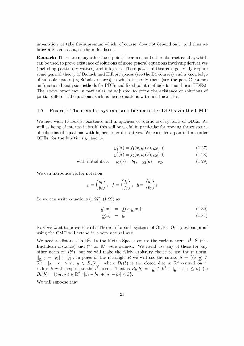
Proposition 3.1. Suppose that P (x, y) and Q(x, y) are Lipschitz continuous in xand y and R(x, y, z) is continuous and Lipschitz continuous in z. Then(a) There is a characteristic projection through each point of the plane, and theycan only meet at critical points (ie points where P and Q are both zero).(b) Given a point p ∈ Σ, the characteristic through p lies entirely on Σ.

47

Proof

(a) This is exactly the same as in Section 2.1, as (3.3)(a),(b) is an autonomous systemand, if P 6= 0, reduces to dy

dx = QP , which has a unique solution for given initial

data. We can then find z uniquely along y = y(x) from

dz

dx=R(x, y(x), z)

P (x, y(x)).

(b) (This is fiddly.) Let (x(t), y(t), z(t)) be the characteristic through p and set

Σ(t) = z(t)− f(x(t), y(t)).

Then to prove that the characteristic lies on the surface Σ we must show thatΣ(t) ≡ 0. To do this we will show that Σ(t) satisfies an IVP which has the uniquesolution zero so that Σ(t) = 0 for all t.

From (3.3) and the chain rule

dΣ

dt= R(x(t), y(t), z(t))− ∂f

∂xP (x(t), y(t))

−∂f∂yQ(x(t), y(t)),

while from (3.1)

R(x(t), y(t), f(x(t), y(t))− ∂f

∂xP (x(t), y(t))− ∂f

∂yQ(x(t), y(t)) = 0.

Subtract thesedΣ

dt= R(x, y, z)−R(x, y, f)

Now put f = z − Σ, then the RHS here is a function F (Σ(t), t) for some F withF (0, t) = 0. Furthermore, if the point p is (x(0), y(0), z(0)) then Σ(0) = 0.Thus we have an ODE for Σ(t), with given initial value, and the RHS is continuousand is Lipschitz continuous in Σ (check!), so the IVP has a unique solution. ButΣ(t) = 0 is a solution, so it is the only one. Therefore, Σ = 0 all along Γ, and Γlies on the solution surface. Q.E.D.

Thus the solution surface Σ is generated by a collection of characteristics.

3.2.1 Examples of characteristics

We need to gain proficiency in calculating characteristics.

48

(a) Calculate the characteristics for the PDE:

x∂z

∂x+ y

∂z

∂y= z.

From (3.3) write down the characteristic equations and solve them:

dx

dt= P = x; x = Aet

dy

dt= Q = y; y = Bet

dz

dt= R = z; z = Cet

with A, B, C constants (trivial to solve).

(b) Calculate the characteristics for the PDE:

y∂z

∂x+∂z

∂y= z.

dx

dt= y; x = Bt+

t2

2+A

dy

dt= 1; y = B + t

dz

dt= z; z = Cet.

with A, B, C constants. To solve this system, pass over the first, solve the second,then come back to the first and third. (I am adopting a convention to introducethe constants A,B,C in the first, second and third of the characteristic equationsrespectively.)

In general solving the characteristic equations needs experience and luck; there isn’t ageneral algorithm.

3.3 The Cauchy problem

A Cauchy Problem for a PDE is the combination of the PDE together with boundarydata that, in principle, will give a unique solution, at least locally. We will look forsuitable data and determine the domain on which the solution is uniquely determined.

Suppose we are given the solution z of (3.1) along a curve γ0 (the data curve) in the(x, y)-plane. This produces a curve γ in space (the initial curve):

49

z

x

y

γ0(s) = (x(s), y(s), 0))

γ(s) = (x(s), y(s), z(s))

Figure 3.2: Geometry of the Cauchy problem.

We introduce a parameter s along γ so it is (x(s), y(s), z(s)), while γ0 is the projection(x(s), y(s), 0), and we will assume x, y, z are continuously differentiable. Then, to solve(3.1), we construct the solution surface Σ by taking the characteristics through the pointsof γ (because Proposition 3.1(b) tells us that the solution surface is generated by thesecharacteristics) . Thus the method of solution, the method of characteristics, is

(i) Parametrise γ as (x(s), y(s), z(s)).

(ii) Solve∂x

∂t= P

∂y

∂t= Q

∂z

∂t= R

for (x(t, s), y(t, s), z(t, s)) with data x(0, s) = x(s); y(0, s) = y(s); z(0, s) = z(s).

then, knowing (x(t, s), y(t, s), z(t, s)), we have found Σ in parametric form. We wouldlike to find the solution explicitly, that is z in terms of x and y, a question we will explorebelow, and there is a restriction on the data for the method to work, also to be foundlater.

3.4 Examples

(a) Solve

y∂z

∂x+∂z

∂y= z,

with z(x, 0) = x for 1 ≤ x ≤ 2.

50

z

x

γ

γ0

y

2

1

12

Figure 3.3: The data curve for this problem

We introduce a parameter s for the data, say γ(s) = (s, 0, s), for 1 ≤ s ≤ 2, andthen solve the characteristic equations (done in section 3.2.1) with this as data att = 0

x = Bt+t2

2+A; x(0, s) = A = s

y = B + t; y(0, s) = B = 0

z = Cet; z(0, s) = C = s

So, C = s, B = 0, A = s and the parametric form of the solution is

x = s+ 12 t

2

y = tz = set

(3.4)

for 1 ≤ s ≤ 2.

(b) (From Ockendon et al) Solve

x∂z

∂x+ y

∂z

∂y= (x+ y)z (3.5)

with z = 1 on the segment of the circle (x− 2)2 + y2 = 2, y ≥ 0.

So we can take γ(s) = (2 −√

2 cos s,√

2 sin s, 1), s ∈ [0, π], and solve the charac-teristic equations:

∂x

∂t= P = x; x = Aet; A = (2−

√2 cos s)

∂y

∂t= Q = y; y = Bet; B =

√2 sin s

51

∂z

∂t= R = (x+ y)z = ((2−

√2 cos s+

√2 sin s)et)z.

We can integrate the final equation to get

log |z| = ((2−√

2 cos s+√

2 sin s)et) + C; C = −(2−√

2 cos s+√

2 sin s).

So the parametric form of the solution is

x = (2−√

2 cos s)et

y = (√

2 sin s)et

z = exp[((2−√

2 cos s+√

2 sin s)(et − 1)]

(3.6)

3.5 Domain of definition

Where is the solution determined uniquely by the data? This is the domain of definitionand is the region in the (x, y)-plane where the solution surface is uniquely determinedand is given explicitly as z = f(x, y).

Bounded Initial Data:

In general the initial curve could be bounded or semi-infinite. The solution surface isswept out by the characteristics through the initial curve, so the solution will be definedin the region swept out by the projections of the characteristics through the initial curve.In particular if the initial curve is bounded, the domain of definition will be bounded bythe projections of the characteristics through the end points of the initial curve.

Blow up:

The method of characteristics reduces the PDE (3.1) to a system of ODEs. As we havealready seen nonlinear ODEs can give rise to solutions which blow up, so the same mustbe true of non linear PDEs, even if those that are semi-linear.

Explicit solution: We want z as a function of x and y, so we need to be able toeliminate t and s in favour of x and y, at least in principle. For this, recall from Prelimsthe definition of the Jacobian:

J(s, t) =∂(x, y)

∂(t, s)= det

(xt ytxs ys

). (3.7)

Now ifx = x(t, s), and y = y(t, s)

are continuously differentiable functions of t and s in a neighbourhood of a point, thena sufficient condition to be able to find unique continuously differentiable functions

t = t(x, y) and s = s(x, y)

in some neighbourhood of the point, is that J be non-zero at the point. We can thensubstitute into z = z(t, s) to get

z = z(t(x, y), s(x, y)) = f(x, y),

52

a continuously differentiable function of x and y as required. This comes from a resultknown as the Inverse Function Theorem. We will have to take it on trust, but it is thetwo dimensional equivalent of the one dimensional result you saw in Analysis in Prelims- where the function f has a differentiable inverse if f has a non zero derivative.

Thus we require first that J(s, 0) 6= 0 on the initial curve. If this is so, then the problemhas a unique explicit solution, at least close to the initial curve. Then, we can continueto extend the solution away from the curve so long as J 6= 0 and the solution does notblow up.

This fails if the data curve touches a characteristic projection. For

J(s, 0) = det

(xt ytxs ys

)= det

(P Qxs ys

). (3.8)

So if, for some s, J(s, 0) = 0 then, if a dash denotes differentiation with respect to s onγ0 = (x(s), y(s), 0) , we have

P (x, y)y′ −Q(x, y)x′ = 0, (3.9)

so the data curve is tangent to the projection of the characteristic at that point.

Typically away from the initial curve we will only have J = 0 if the characteristics crosseach other (so that uniqueness fails) and for semi-linear problems this can only happenat critical points.

Examples:

Example (a) : Let us determine the domain of definition for the example of section3.4(a):

The solution surface is swept out by the characteristics through γ, so has edges given bythe characteristics through the ends of γ, which are at s = 1 and s = 2.

At s = 1, the characteristic projection is

x = 1 +1

2t2; y = t so x = 1 +

1

2y2;

at s = 2 it’s

x = 2 +1

2t2 y = t so x = 2 +

1

2y2

53

0.0 0.5 1.0 1.5 2.0 2.5 3.0-2

-1

0

1

2

x=1 x=2

x = 1 + 12y

2

x = 2 + 12y

2

Figure 3.4: The domain of definition for this problem

so the solution surface lies above the region

1 +1

2y2 ≤ x ≤ 2 +

1

2y2 (3.10)

54

and these curves don’t meet .

It is easy to see from (3.4) that the solution can be given explicitly as z(x, y) = (x− 12y

2)ey

for 1 + 12y

2 ≤ x ≤ 2 + 12y

2.

Thus the solution does not blow up and can be given explicitly. Therefore (3.10) givesthe domain of definition. Or we could calculate J which is never zero.

Example (b): Now look at the example of section 3.4(b); First consider

J = det

((2−

√2 cos s)et (

√2 sin s)et

(√

2 sin s)et (√

2 cos s)et

)= 2e2t(1−

√2 cos s),

This vanishes when s = π4 , that is along the characteristic projection y = x, which

touches the data curve at (1, 1). So we will restrict the data curve to s ∈ [0, π/4).The data curve starts at s = 0, so the solution surface will have an edge given by thecharacteristic through the end of γ at s = 0 and at s = 0 the characteristic projection isy = 0. But the domain of definition is swept out by the projections of the characteristicsthrough γ. So the domain of definition is 0 ≤ y < x.

Remark: More generally if the data curve and characteristic projection coincide then,if the initial curve γ is a characteristic so that z(s) satisfies dz

ds = R, there will be aninfinity of solutions through γ, while otherwise there will be no solution.

For, if γ is a characteristic, then let C be any curve through γ whose projection is nowheretangent to a characteristic projection. Then there is a solution surface through C. Butthis was any C so there is an infinity of solutions. On the other hand, if the data curveis a characteristic projection, then there can only be a solution if γ = (x(s), y(s), z(s))is a characteristic, as if the solution surface is z = f(x, y), then z(s) = f((x(s), y(s)) so,using the chain rule,

dz

ds=dx

dsfx +

dx

ds= Pfx +Qfyfy = R.

So, returning to our example above, if one continues along the data curve from s = π4

there will be problems as each characteristic meets the data curve in two points, so theinitial data is likely to be inconsistent. If one changes the data curve to continue tothe left of y = x (for example the curve with the small dashes in the diagram) then itis likely there would only be problems on the characteristic y = x. But if we continuethe data curve to include a section of the line y = x (curve with larger dashes in thediagram) the problem is likely to have no solution.

55

0 1 2 3 40.0

0.5

1.0

1.5

2.0

2.5

3.0

Figure 3.5: Different data curves for problem (3.5)

Example (c): Consider the PDE

∂z

∂x+∂z

∂y= z2,

with z(x, 0) = 1.

parametrise the initial curve as (s, 0, 1). Then the solutions of the characteristics are:x = t+ s, y = t, z = 1

1−t , so z = 11−y which blows up at y = 1.

3.6 Cauchy data and the Cauchy Problem:

We have seen that a necessary condition on the data for the solution to exist close tothe initial curve is that on γ0

P (x, y)y′ −Q(x, y)x′ 6= 0. (3.11)

If it holds, we call the data Cauchy data.

Thus the Cauchy Problem is the PDE (3.1) with Cauchy data.

3.7 Discontinuities in the first derivatives

The characteristic projections have another property. They are the only curves acrosswhich the solution surface can have discontinuities in the first derivatives. For, supposethat γ is the curve (x(s), y(s), z(s)) in the solution surface, across which there are discon-tinuities in the first order partial derivatives but z is continuous. Use the superscript ±to denote the solution on either side of γ and denote the jumps in the partial derivative

56

by [zx]+− = z+x − z−x and [zy]

+− = z+

y − z−y . Then differentiating each solution along γ,and also using (3.1)

dz+

ds= z+

x

dx

ds+ z+

y

dy

ds, (3.12)

R = Pz+x +Qz+

y . (3.13)

and

dz−

ds= z−x

dx

ds+ z−y

dy

ds, (3.14)

R = Pz−x +Qz−y . (3.15)

But z is continuous across γ, so dz+

ds = dz−

ds , and subtracting, we see that

0 = [zx]+−dx

ds+ [zy]

+−dy

ds, (3.16)

0 = P [zx]+− +Q[zy]+−. (3.17)

Thus for there to be a non-zero jump, the solution of these simultaneous equations mustbe nonzero, so the determinant of the coefficients must be zero. That is

0 = det

(P Qdxds

dyds

), (3.18)

so that the projection of the curve must be a characteristic projection. That it is acharacteristic curve now follows from (3.12) and (3.13). See problem sheet 3 for anexample of this.

Figure 3.6: The curve γ.

57

3.8 General Solution

Another problem we could have considered, is what is the most general solution of (3.1)?Just as we expect the most general solution of an ODE to have n arbitrary constants, sowe expect the most general solution of a PDE of order n to have n arbitrary functions.

For example: The first order PDE ∂z∂x(x, y) = 0, has the most general solution z = f(y)

where f is an arbitrary function.

58

4 Second order semi-linear PDEs

4.1 Classification

In this section, we are interested in second-order PDEs of the following form:

a(x, y)uxx + 2b(x, y)uxy + c(x, y)uyy︸ ︷︷ ︸principal part

= f(x, y, u, ux, uy). (4.1)

This PDE is said to be linear if f is linear in u, ux, uy, otherwise it is said to semi-linear.(If the coefficients a, b, c also depend on u, ux, uy it is said to be quasi-linear. We willconsider only semi-linear equations.) You have seen the following examples in Prelims:

uxx + uyy = 0 Laplace’s equation

uxx − uyy = 0 wave equation if y = ct

uxx − uy = 0 heat equation if y = t/κ.

Equations that are linear (in the dependent variable) have solutions that can be combinedby linear superposition (taking linear combinations). In general PDEs that are nonlinear(for example where f , above, depends nonlinearly on u or its derivatives) do not havesolutions that are superposable.

We will assume throughout that functions are suitably differentiable.

4.1.1 The idea:

In this section, the key idea is to change coordinates so as to simplify the principal part.So we make the change of variables

(x, y)→ (ϕ(x, y), ψ(x, y));

with non vanishing Jacobian (basically this ensures that the map is locally invertible):

∂(ϕ,ψ)

∂(x, y)= ϕxψy − ϕyψx 6= 0.

We will abuse the notation a little and write (the solution) u as either a function of(x, y) or (ϕ,ψ) as required.

For the change in the partials, we calculate

ux = uϕϕx + uψψx; uy = uϕϕy + uψψy

59

then

uxx = uϕϕϕ2x + 2uϕψϕxψx + uψψψ

2x + uϕϕxx + uψψxx

uxy = uϕϕϕxϕy + uϕψ(ϕxψy + ψxϕy) + uψψψxψy + uϕϕxy + uψψxyuyy = uϕϕϕ

2y + 2uϕψϕyψy + uψψψ

2y + uϕϕyy + uψψyy

(4.2)

so that (4.1) becomes

A(ϕ,ψ)uϕϕ + 2B(ϕ,ψ)uϕψ + C(ϕ,ψ)uψψ = F (ϕ,ψ, u, uϕuψ) (4.3)

withA = aϕ2

x + 2bϕxϕy + cϕ2y

B = aϕxψx + b(ϕxψy + ϕyψx) + cϕyψyC = aψ2

x + 2bψxψy + cψ2y .

(4.4)

(Beware, F will include lower order derivatives from (4.2).) In a matrix notation (4.4)is (check!)

(A BB C

)=

(ϕx ϕyψx ψy

)(a bb c

)(ϕx ψxϕy ψy

)so that, taking determinants,

(AC −B2) = (ac− b2)(ϕxψy − ψxϕy)2 = (ac− b2)

(∂(ϕ,ψ)

∂(x, y)

)2

. (4.5)

(We could obtain (4.5) directly from (4.4) but the matrix notation makes the computa-tion simpler.) Now (4.5) leads to a classification of second-order linear PDEs:

4.1.2 The Classification

Second-order linear PDEs are classified into three types as follows:

1. ac < b2 hyperbolic: e.g. wave equation;

2. ac > b2 elliptic: e.g. Laplace equation;

3. ac = b2 parabolic: e.g. heat equation.

So, by (4.5) the class of the equation is invariant under transformations with non-vanishing Jacobian.

We shall look at the classification in terms of the quadratic polynomial

a(x, y)λ2 − 2b(x, y)λ+ c(x, y) = 0. (4.6)

Note: We will assume that a 6= 0, in the domain under consideration. If a = 0 but c 6= 0,we can swap the roles of x and y.

60

Case 1: hyperbolic type

So ac < b2 and the quadratic has distinct real roots λ1, λ2, say. So

a(x, y)

(dy

dx

)2

− 2b(x, y)dy

dx+ c(x, y) = 0. (4.7)

is equivalent tody

dx= λ1(x, y),

dy

dx= λ2(x, y). (4.8)

Suppose these equations have solutions ϕ(x, y)=constant, ψ(x, y) =constant, respec-tively. Set as change of variables

ϕ = ϕ(x, y), ψ = ψ(x, y).

Then, on ϕ(x, y)=constant,

ϕx + ϕydy

dx= 0

so thatλ1ϕy = −ϕx

and thusA(ϕ,ψ) = a(x, y)(ϕx)2 + 2b(x, y)ϕxϕy + c(x, y)(ϕy)

2 = 0,

and analogously C(ϕ,ψ) = 0. But λ1 6= λ2, so ϕxϕy6= ψx

ψy, and from (4.5) B 6= 0. Divide

(4.3) by B to obtain the equation in the form

uϕψ = G(ϕ,ψ, u, uϕ, uψ). (4.9)

This is the normal form (or canonical form) for a hyperbolic equation; the equation(4.7) is the characteristic equation; ϕ, ψ are characteristic variables; curves on which ϕor ψ are constant are characteristic curves. We can often solve (4.9) explicitly.

Examples:

(a)uxx − uyy = 0.

We already know how to solve this, but let us apply the method. So

a = 1, b = 0, c = −1, and λ2 − 1 = 0.

We can takeλ1 = 1, λ2 = −1

and solve (4.8)y′(x) = 1 y′(x) = −1

61

to getϕ = x− y ψ = x+ y.

(There is clearly lots of choice at this stage.) The equation has become

uϕψ = 0,

which we solve at once byu = f(ϕ) + g(ψ),

a solution known from Prelims. So the characteristic curves of the wave equationare x+ ct=const and x− ct =const.

(b) An example with data: solve

xuxx − (x+ y)uxy + yuyy +(x+ y)

(y − x)(ux − uy) = 0, for y 6= x

with

u =1

2(x− 1)2, uy = 0 on y = 1.

Problem is hyperbolic provided x 6= y (check). The quadratic (4.6) is

xλ2 + (x+ y)λ+ y = 0

= (λ+ 1)(xλ+ y);

so chooseλ1 = −1 λ2 = −y

x

and solvey′(x) = −1; y′(x) = −y

x,

by x+ y = const; xy =const, so put

ϕ = x+ y; ψ = xy.

Calculateux = uϕ + yuψ

uy = uϕ + xuψ

so thatuxx = uϕϕ + 2yuϕψ + y2uψψ

uxy = uϕϕ + xuϕψ + yuϕψ + xyuψψ + uψ

uyy = uϕϕ + 2xuϕψ + x2uψψ.

(It is always better to calculate the derivatives directly, rather than trying toremember formulae.)

62

Now the PDE becomes

0 = x[uϕϕ + 2yuϕψ + y2uψψ]

−(x+ y)[uϕϕ + (x+ y)uϕψxyuψψ + uψ]

+y[uϕϕ + 2xuϕψ + x2uψψ]

+(x+ y)uψ

= (4xy − (x+ y)2)uϕψ

souϕψ = 0

and the solution is

u = f(ϕ) + g(ψ) = f(x+ y) + g(xy).

To impose the data, calculate

uy = f ′(x+ y) + xg′(xy)

so on y = 1,

u = f(x+ 1) + g(x) =1

2(x− 1)2

uy = f ′(x+ 1) + xg′(x) = 0.

Differentiate the first:f ′(x+ 1) + g′(x) = x− 1

and solve simultaneously with the second:

g′(x) = −1,

and integrate to findg(x) = −x+ c.

Substitute back in u(x, 1):

f(x+ 1) =1

2(x− 1)2 + x− c =

1

2(x+ 1)2 − x− c,

so

f(x) =1

2x2 − x+ 1− c.

Finally

u = f(x+ y) + g(xy) =1

2(x+ y)2 − (x+ y) + 1− xy.

63

Case 2: elliptic type

Now ac > b2 so (4.6) has a complex conjugate pair of roots, and the integral curves of

y′(x) = λ(x, y); y′(x) = λ(x, y)

are in complex conjugate pairs, ϕ(x, y) =const; ψ(x, y) = ϕ(x, y) =const. Then A =C = 0, B 6= 0 and the equation becomes

uϕϕ = G(ϕ, ϕ, u, uϕ, uϕ).

Introduce new variables, ζ, η, given by ϕ = ζ + iη, ϕ = ζ − iη, to obtain the normalform for an elliptic equation (check):

uζζ + uηη = H(ζ, η, u, uζ , uη), (4.10)

which closely resembles Laplace’s equation.

Example: Classify and reduce to normal form the PDE

yuxx + uyy = 0, for y > 0.

ac− b2 = y so the equation is elliptic when y > 0.

The characteristic equation isy(y′)2 + 1 = 0

that isy1/2y′ = ±i,

so integrating2y3/2 ∓ 3ix = const.

So take as variables ζ = 2y3/2; η = 3x. Making the substitution, we find that

3ζ(uζζ + uηη) + uη = 0,

but ζ 6= 0 so the normal form is

uζζ + uηη = −uζ3ζ.

Case 3: parabolic type

Now ac = b2 so (4.6) has a repeated root λ(x, y). Solve y′(x) = λ(x, y) for one newcoordinate ϕ, and pick any ψ with

ϕxψy − ϕyψx 6= 0 (4.11)

64

as the other, then A = 0 so B2 = AC = 0. But C 6= 0, as ψ =const is not a characteristiccurve by (4.11), so we get the normal form for a parabolic equation:

uψψ = G(u, ϕ, ψ, uϕ, uψ),

which closely resembles the heat equation.

Example:

Classify and reduce to normal form the equation

x2uxx + 2xyuxy + y2uyy = 0 for x > 0. (4.12)

The relevant quadratic is

x2λ2 − 2xyλ+ y2 = 0 = (xλ− y)2

which has equal roots, so this equation is parabolic; λ = yx so solve

dy

dx=y

x, to get, for example, ϕ =

y

x

and take, for example, ψ = x. Calculate

ux = − y

x2uϕ + uψ

uy =1

xuϕ

so that

uxx =y2

x4uϕϕ − 2

y

x2uϕψ + uψψ + 2

y

x3uϕ

uxy = − y

x3uϕϕ +

1

xuϕψ −

1

x2uϕ

uyy =1

x2uϕϕ.

The equation becomes

x2

[y2

x4uϕϕ +

2y

x2uϕψ + uψψ +

2y

x3uϕ

]+

+ 2xy

[− y

x3uϕϕ +

1

xuϕψ −

1

x2uϕ

]+ y2

[1

x2uϕϕ

]= x2uψψ = 0 (4.13)

so the normal form isuψψ = 0

with general solution u = F (ϕ) + ψG(ϕ). In terms of the original variables this is:

u = F(yx

)+ xG

(yx

). (4.14)

65

NB Very often, a question like this will be phrased in the form ‘Classify and reduce tonormal form the equation (4.12) and show that the general solution can be written as(4.14)’. Therefore candidates for ϕ and ψ are proposed by the question itself.

A warning example:

The type can change e.g. classify the equation

uxx + yuyy = 0.

Thenλ2 + y = 0, λ2 = −y,

and this is:

� elliptic in y > 0,

� parabolic at y = 0,

� hyperbolic in y < 0.

4.2 Characteristics:

The characteristics of second order semi-linear PDEs have analogous properties to thecharacteristic projections of first order semi-linear PDEs. (Note the difference in termi-nology.)

Firstly, if there are discontinuities in the second derivatives of a solution across a givencurve, then that curve must be a characteristic curve. To see this, suppose that the curveΓ, given parametrically by (x(s), y(s)), is a curve across which there are discontinuitiesin the second derivatives of the solution. Let u+

xx etc denote values on one side of Γand u−xx denote values on the other side of Γ. Then differentiating ux(x(s), y(s)) anduy(x(s), y(s)) along Γ, and noting that u, ux, uy are continuous across the curve,

duxds

=dx

dsu±xx+

dy

dsu±xy

duyds

=dx

dsu±yx +

dy

dsu±yy

and also f(x, y, u, ux, uy) = a(x, y)u±xx+ 2b(x, y)u±xy + c(x, y)u±yy.

Subtracting the ‘minus’ equation from the ‘plus’ equation

0 =dx

ds[uxx]+−+

dy

ds[uxy]

+−

0 =dx

ds[uyx]+− +

dy

ds[uyy]

+−

0 = a(x, y)[uxx]+−+ 2b(x, y)[uxy]+− + c(x, y)[uyy]

+−,

66

where [uxx]+− = u+xx − u−xx denotes the jump in uxx across Γ, etc. If there are to be

discontinuities in the second derivatives, then this set of equations in the jumps musthave a nonzero solution, so that the determinant of the coefficients must be zero. Thus

a(x, y)

(dy

ds

)2

− 2b(x, y)dx

ds

dy

ds+ c(x, y)

(dx

ds

)2

= 0, (4.15)

so Γ is a characteristic.

Furthermore, under suitable smoothness conditions, the Cauchy problem for a secondorder semi-linear PDE, where u and ∂u

∂n are given along a curve Γ, will have a uniquelocal solution provided Γ is nowhere tangent to a characteristic curve. This result isbeyond the scope of this course and will be investigated further in the Part B course,Applied PDEs. It can be seen that it is necessary that Γ is not a characteristic curve, asif u exists then it must have unique second order partial derivatives along Γ and exactlyas above this can only be true when Γ is not a characteristic curve.

Remark: Our previous work carried the implicit assumption that a 6= 0. Note that(4.15) gives a method of calculating the characteristic curves if a = 0. In particular ifa = 0 and c = 0 then the characteristic curves are x =const, y =const.

4.3 Type and data: well posed problems

We want to say something about the notion of well posedness and its connection withtype. Our examples are mostly based on knowledge acquired in Prelims.

A problem, consisting of a PDE with data, is said to be well posed if the solution:

� exists

� is unique

� depends continuously on the data.

Recall that, in Section 1.5, we said that a solution of a DE is continuously dependenton the data if the error in the solution is small provided the error in the initial data issmall enough.. We then gave a precise definition for ODEs. We now want to extendthis definition to PDEs. Data can be given in different ways, so to be precise we willconsider a problem where u(x, y) is the solution of a certain PDE in a bounded subset ofthe plane D, with u given on some curve Γ. Then we will say that the solution dependscontinuously on the data if :

∀ε > 0 ∃δ > 0 such that if ui, i = 1, 2, are solutions with ui = fi on Γ then

supΓ|f1 − f2| < δ ⇒ sup

D|u1 − u2| < ε.

67

The definition extends in a fairly obvious way to other types of data. (Note that thereare plenty of other ‘distances ’ we could use in place of taking the sup, but that is whatwe will use here.)

Of the three requirements for well posedness it is existence which is the hardest to obtain.In Prelims solutions were found for a number of linear problems, either by making achange of variables and then integrating, or by using separation of variables and Fourierseries. Anything more than this is beyond the scope of this course. Uniqueness ofsolution was also proved for a number of linear problems (even when you didn’t knowif the solution existed). Proving uniqueness and continuous dependence on the data ismuch easier for linear problems as we can then start out by looking at the differencebetween two solutions, which will then be the solution of some suitable problem. Later wewill look at the linear equations Poisson’s equation and the heat equation and state andprove the maximum principle, which will enable us to prove uniqueness and continuousdependence for suitable boundary data.

But first we need to consider what data might be appropriate. In Prelims you consideredthree particular PDEs, each with a different type of data which arose from the particularphysical problem they modelled. These are summarised in the table below. It turns outthat there are mathematical as well as physical reasons why each problem had a differenttype of data. So first we will look at some of these problems and consider which may bewell posed.

68

Som

eM

od

els

from

Pre

lim

s:

PD

EM

od

els

Bou

nd

ary

con

dit

ion

s

Wav

eE

qu

ati

on

:c2uxx−utt

=0

Wav

eson

ast

rin

g;u

,∂u∂t

give

nt

=0

(IB

VP

)H

yp

erb

olic

(In

fin

ite

stri

ng)

ugi

ves

dis

pla

cem

ent

∂u∂t

give

nt

=0;

plu

sen

dp

oint

(IV

P)

con

dit

ion

-sa

yu

=0

aten

ds

(Fin

ite

stri

ng)

Lap

lace

’sE

qu

atio

n:

uxx

+uyy

=0,

Pot

enti

alT

heo

ryor

uor

∂u∂n

give

non

bou

nd

ary

ofD

(BV

P)

Ell

ipti

c(x,y

)∈D

Ste

ady

Hea

t;u

give

sp

oten

tial

orte

mp

erat

ure

Hea

tE

qu

atio

n:

ut

=κuxx

Hea

t;u

give

natt

=0;

(IB

VP

)P

arab

olic

plu

sen

dp

oint

con

dit

ion

s(T

emp

erat

ure

ugi

ves

tem

per

atu

re-u

or∂u∂x

give

nat

end

sin

fin

ite

bar

)

69

Some examples from Prelims: (We will assume that the data is smooth enough forthe following to hold.)

(a) Hyperbolic equation: The IVP and IBVP (initial-boundary-value problem) for thewave equation

uxx − uyy = 0 (ct = y).

For the IVP (modelling an infinite string, where u is the displacement), we knowthe solution is

u =1

2[f(x+ y) + f(x− y)] +

1

2

∫ x+y

x−yg(s)ds, (4.16)

where the data are u(x, 0) = f(x) and uy(x, 0) = g(x), −∞ < x < ∞. This isd’Alembert’s solution of the IVP: it exists, and is unique and, intuitively at least,a small change in ϕ,ψ gives a small change in u (see problem sheet for proof). Sothis problem is well-posed.

For the IBVP (modelling a finite string length L, fixed at each end) consider thedata:

u(x, 0) = f(x), uy(x, 0) = g(x) 0 < x < L

u(0, y) = 0 = u(L, y).

So the boundaries are at x = 0, L. This IBVP is solved using separation of variablesand Fourier series to get a solution

u =∑n

sinnπx

L

(an cos

nπy

L+ bn sin

nπy

L

)with an, bn given in terms of f and g. Uniqueness was shown in Prelims, so thisis the unique solution. If we now appeal to intuition for continuous dependence onthe data this problem is well-posed.

(b) Elliptic equation:The BVP for the Laplace/Poisson’s equation (modelling steadystate heat, for example, where u is the temperature)

uxx + uyy = 0.

Do this first with data at the sides of a square, so 0 ≤ x, y ≤ a with

u(0, y) = u(a, y) = u(x, 0) = 0; u(x, a) = f(x).

Consider separable solutions un = sin nπxa sinh nπy

a , then

u =∑n

ansinh nπy

a

sinh(nπ)sin

nπx

a

70

andf(x) =

∑an sin

nπx

a

which determines the solution as a Fourier series.

Now a different BVP, with data at the circumference of the unit circle:

on r = 1, u = f(θ)

and in polars

urr +1

rur +

1

r2uθθ = 0.

The separable solutions are{ (Arn + B

rn

)(C cosnθ +D sinnθ)

A+B log r, n = 0

Regularity at r = 0 implies

u =1

2a0 +

∞∑1

rn(an cosnθ + bn sinnθ)

and the boundary value at r = 1 requires

1

2a0 +

∑(an cosnθ + bn sinnθ) = f(θ)

which again is solved by Fourier methods.

Uniqueness was proved in Prelims so in each of these cases we have the uniquesolution. It is plausible, but beyond our scope, to show that there is existence ofsolution in general. Later we will prove that there is continuous dependence onthe data. So this problem is well posed

(c) Parabolic equation: The IBVP for the heat equation (modelling heat flow in a barlength L, with the ends held at zero temperature, u is temperature. )

uxx = uy

on the semi-infinite strip where y = t > 0 and 0 < x < L, and data

u(x, 0) = f(x); u(0, y) = 0 = u(L, y).

The relevant separable solutions are

un = sinnπx

Le−

n2π2tL2

so that

u =∑n

an sinnπx

Le−

n2π2

L2 t

71

and the initial value requires

f(x) =∑

an sinnπx

L

which is solved by Fourier methods. The solution exists provided the series for uconverges which it will do for positive t. However, note that for negative t theexponentials grow rapidly with n and there is no reason to expect existence.

Uniqueness for this problem was done in Prelims, so again this is the uniquesolution for positive t. Later we will prove continuous dependence on the data.Thus the problem is well posed forward in time.

(d) What then is not well-posed? We give a few examples:

� BVPs for hyperbolic

e.g. uxx − uyy = 0 on the unit square with data

u(0, y) = u(1, y) = u(x, 0) = 0; u(x, 1) = f(x).

Recall this data gave a well-posed problem for the Laplace equation, but hereif f = 0, then sinnπx sinnπy will do, for any n, while it can be proved thatthere is no solution at all if f 6= 0 (try the Fourier series to see what goeswrong).

� IVPs for elliptic

e.g. uxx + uyy = 0 in the horizontal strip 0 ≤ y ≤ Y , −∞ < x < ∞, withdata

u(x, 0) = 0, uy(x, 0) = f(x).

We know (from the problem sheet) that this data gives continuous depen-dence on the data for the wave equation. But not for Laplace’s equation.For if f(x) = 1

n sinnx it can be seen that u(x, y) = 1n2 sinhny sinnx. But

sup | 1n2 sinhny sinnx| → ∞ as n → ∞, whereas 1/n sinnx → 0. Thus small

changes in the initial data can lead to large changes in the solution. [Moreprecisely: Suppose that there is continuous dependence on the initial dataabout the zero solution. That is: ∀ε > 0, ∃δ > 0 such that

supx∈R|f(x)− 0| < δ ⇒ sup

x∈R,0≤y≤Y|u(x, y)− 0| < ε.

But taking ε = 1, say, there existsN such that for all n > N , sup | 1n2 sinhny sinnx| >

1, but for any δ > 0 we can choose n > N such that | 1n sinnx| < δ, giving acontradiction.

� IBVP for elliptic

e.g. uxx + uyy = 0 on the semi-infinite strip 0 ≤ x ≤ 1, y ≥ 0, with data

u(0, y) = u(1, y) = 0, u(x, 0) = 1, uy(x, 0) = 0.

72

This data gives a well-posed problem for the wave equation. If we try forseparable solutions here, we have un = sinnπx coshnπy so

u =∑n

an sinnπx coshnπy.

Initial conditions need1 =

∑an sinnπx

whencean = 0 n even

=4

nπn odd,

and then

u

(1

2, y

)=∑n

4

(2n+ 1)π(−1)n cosh(2n+ 1)πy,

which does not converge for any y > 0 (because the ”cosh” terms grow rapidlywith n) - there is no solution (strictly speaking, we’ve only shown that thereis no solution of the form considered; we need more).

� The BVP for the heat equation is not well-posed, but we won’t show that.

Again, it is beyond our scope to prove it in this course, but these different be-haviours are universal for the different types of second-order, linear PDEs. Intabulated form, which problems are well-posed?

IVP IBVP BVPHyperbolic yes yes noElliptic no no yesParabolic yes yes no

where the ‘yes’ for parabolic equations are only valid forward in time.

4.4 The Maximum Principle

4.4.1 Poisson’s equation

The normal form for second-order elliptic PDEs is

uxx + uyy = f(x, y, u, ux, uy) (4.17)

73

The operator on the left-hand side is referred to as the Laplacian, for which the symbols∇2u and ∆u are often used as shorthand. Poisson’s equation is a special case of (4.17),in which f depends only on x and y. We have already seen that appropriate boundarydata for (4.17) is to give just one boundary condition on u everywhere on a closed curve.

We will consider the Dirichlet problem where u is given on the boundary of D:

uxx + uyy = f(x, y) in D (4.18)

u = g(x, y) on ∂D. (4.19)

It was shown in Prelims, using the divergence theorem, that if a solution exists, then itis unique. Using the maximum principle we will give another proof of this and also showthat there is continuous dependence on the data. The solution does exist, but apartfrom the particular cases considered in Prelims that is beyond the scope of this course.

Theorem 4.1. (The Maximum principle for Poisson’s equation) Suppose u satisfiesPoisson’s equation everywhere within a bounded domain, D,

uxx + uyy = f(x, y) (x, y) ∈ D, (4.20)

where we have f ≥ 0 in D. Then u attains its maximum value on ∂D.

Proof:

If we denote the boundary of D by ∂D , then as D∪∂D is a closed bounded set, u mustattain its maximum somewhere in D or on its boundary. The proof now proceeds in twoparts.

Suppose first that f > 0 in D.

If u has an interior maximum at some point (x0, y0) inside D, then the following condi-tions must be satisfied at (x0, y0):

ux = uy = 0, uxx ≤ 0, uyy ≤ 0.

But, if f is strictly positive, (4.20) implies that it is impossible for both uxx and uyy tobe non positive (they sum to f). Hence u cannot have an interior maximum within D,so it must attain its maximum value on the boundary ∂D.

Suppose now that we only have f ≥ 0 in D. We perturb u to get a function v whichsatisfies Poisson’s equation with the right hand side strictly positive, so we can applythe first part of the proof.

Consider the functionv(x, y) = u(x, y) +

ε

4(x2 + y2),

where ε is a positive constant.

Thenvxx + vyy = f + ε > 0

74

in D. So using the result just proved, v attains its maximum value on ∂D.

Now, suppose that the maximum value of u on ∂D is M and the maximum value of(x2 + y2) on ∂D is R2 , then the maximum value of v on ∂D (and thus throughout D)is M + (ε/4)R2 . In other words, the inequality

u+ε

4(x2 + y2) = v ≤M +

ε

4R2

holds for all (x, y) ∈ D. Letting ε → 0, we see that u ≤ M throughout D, i.e. that uattains its maximum value on ∂D.

It obviously follows (by using the above result with u replaced by −u) that, if f ≤ 0 inD, then u attains its minimum value on ∂D.

In the case f = 0, u therefore attains both its maximum and minimum values on ∂D.This is an important property of Laplace’s equation.

Remark: (a) The result also holds if f is also a function of u, provided f(x, y, u) ≥ 0in D for all u.

(b) Note that if f > 0 then the maximum of u will be attained only on the boundary,whereas if f ≤ 0 the maximum may also be attained within the interior of D as well ason the boundary.

Corollary 4.2. (a) Consider the Dirichlet problem (4.18), (4.19). Then if the solutionexists, it is unique.

(b) The Dirichlet problem (4.18), (4.19) has continuous dependence on the data.

Proof: (a) Suppose that u1, u2 are two solutions, so u = u1 − u2 satisfies

uxx + uyy = 0 in D (4.21)

u = 0 on ∂D. (4.22)

By (4.21) the maximum and minimum of u occur on ∂D, so by (4.22) u ≤ 0 and u ≥ 0in D. Thus u = 0 in D as required.

(b) We have to prove that for all ε > 0 there exists δ > 0 such that if ui, i = 1, 2 aresolutions with boundary data gi, then

sup(x,y)∈∂D

|g1(x, y)− g2(x, y)| < δ ⇒ sup(x,y)∈D

|u1(x, y)− u2(x, y)| < ε.

By linearity u = u1 − u2 satisfies

uxx + uyy = 0 in D (4.23)

u = g1 − g2, on ∂D. (4.24)

We now apply the maximum principle to see that u ≤ max(x,y)∈∂D(g1−g2), and applyingthe same result to −u, −u ≤ max(x,y)∈∂D −(g1 − g2).

75

Hence in D

|u1 − u2| ≤ max(x,y)∈∂D

|g1 − g2|, (4.25)

so we may take δ = ε.

76

4.4.2 The heat equation

In parabolic PDEs it is usually the case that one independent variable representstime, so we now use x and t as independent variables instead of x and y. Thenormal form for second-order parabolic equations is

uxx = F (x, t, u, ut, ux)

and specific examples include the inhomogeneous heat equation, often called thediffusion equation:

ut = uxx + f(x, t).

and the reaction-diffusion equation

ut = uxx + f(x, t, u),

Well posed boundary data: Typical boundary data for a diffusion equation areto give an initial condition for u at t = 0 and one boundary condition on each oftwo curves C1 and C2 in the (x, t)-plane that do not meet and are nowhere parallelto the x-axis.

For example: The inhomogeneous heat equation

ut = uxx + f(x, t)

is a simple model for the temperature u(x, t) in a uniform bar of conductive ma-terial, with heat source f(x, t), where x is position and t is time. Suppose the baris of length L, its initial temperature is given via u0(x), and its ends are kept atzero temperature. Then the initial and boundary conditions are

u = u0(x) at t = 0, u = 0 at x = 0; u = 0 at x = L.

If, instead of being held at constant temperature, an end is insulated, then theDirichlet boundary condition, u = 0, there is replaced by the Neumann boundarycondition, ux = 0. Alternatively , the boundary conditions at x = 0 and x = Lmay, in general, be replaced by conditions at moving boundaries, say x = x1(t)and x = x2(t).

Theorem 4.3. (The Maximum principle for the heat equation) Suppose that u(x, t)satisfies the inhomogeneous heat equation

ut − uxx = f(x, t) (4.26)

in a region Dτ bounded by the lines t = 0, t = τ > 0, and two non-intersectingsmooth curves C1 and C2 that are nowhere parallel to the x-axis. Suppose also thatf ≤ 0 in Dτ . Then u takes its maximum value either on t = 0 or on one of thecurves C1 or C2 .

77

Proof:

The proof is similar to that for Poisson’s equation.

Suppose first that f < 0 in Dτ . At an internal maximum inside Dτ , u must satisfy

ux = ut = 0 uxx ≤ 0, (utt ≤ 0).

On the other hand, if u has a maximum at a point on t = τ , then there it mustsatisfy

ux = 0, ut ≥ 0, uxx ≤ 0.

With f assumed to be strictly negative, both of these lead to contradictions, and itfollows that u must take its maximum value somewhere on ∂Dτ but not on t = τ .We are done.

Suppose now that f ≤ 0, then define

v(x, t) = u(x, t) +ε

2x2,

where ε is a positive constant. Then v satisfies

vt − vxx = f(x, t)− ε < 0

in Dτ . So by the earlier step v takes its maximum value on ∂Dτ but not on t = τ .

Now if the maximum value of u over these three portions of ∂Dτ is M , and themaximum value of |x| on C1 and C2 is L, then

u ≤ v ≤ L2ε

2+M.

Now we let ε → 0 and conclude that u ≤ M , i.e. u takes its maximum value on∂Dτ but not on t = τ

If f ≥ 0 in Dτ , then a similar argument shows that u attains its minimum valueon ∂Dτ but not on t = τ . Thus, for the homogeneous equation (the heat equation)u attains both its maximum and its minimum values on ∂Dτ but not on t = τ .

Remark: (a) Again the result also holds if f is also a function of u, providedf(x, t, u) ≤ 0 in Dτ for all u.

(b) Physical interpretation: In a rod with no heat sources the hottest and thecoldest spot will occur either initially or at an end. (Because heat flows from ahotter area to a colder area.)

Corollary 4.4. Consider the IBVP consisting of (4.26) in Dτ with u given on∂Dτ\{t = τ}. Then if the solution exists, it is unique and depends continuouslyon the initial data.

78

Proof: As for Poisson’s equation (see problem sheet).

Sketch: Suppose that ui (i = 1, 2) are solutions of (4.26) in Dτ with data

ui = gi on C1, ui = hi on C2, ui(x, 0) = ki(x) for x between C1 and C2 .

Let u = u1 − u2, g = g1 − g2, h = h1 − h2, k = k1 − k2. Then u satisfies (4.26)with f = 0, and u = g on C1, u = h on C2, u(x, 0) = k(x) for x between C1 andC2 . Thus u and −u take their maximum values on ∂Dτ\{t = τ}. Hence

supDτ

u ≤ max{sup g, suph, sup k}

andsupDτ

−u ≤ max{sup−g, sup−h, sup−k}.

SosupDτ

|u| ≤ max{sup |g|, sup |h|, sup |k|},

and continuous dependence follows. In particular, if g = h = k = 0 then u = 0and uniqueness follows.

79

5 Where does this course lead?

The course leads to DEs2, where, among other topics, boundary value problems forODEs are discussed. Further discussion of differential equations comes in the PartB courses ‘Non-linear Systems’ and ‘Applied Partial Differential Equations’. Theuse of abstract methods such as the Contraction Mapping Theorem to investigatethe solutions of differential equations is taken further in various C4 courses, whichrequire some knowledge of Banach and Hilbert spaces.

The techniques taught in DEs1 and DEs2 will be useful in various applied mathscourses such as the Part A short course ‘Modelling in Mathematical Biology’ andthe Part B courses ‘Mathematical Ecology and Biology’, ‘Viscous Flow’ and ‘Wavesand Compressible Flow’.

5.1 Section 1

Fixed point results such as the CMT provide very powerful methods for provingexistence of solution for ODEs and PDEs. For PDEs we have to work in Banachspaces of functions rather than Rn. For example for parabolic equations such asthe reaction-diffusion equation:

ut = uxx + f(t, u),

with suitable boundary data, our proof of Picard’s theorem can be extended toprove local existence (in t), provided f is continuous and is Lipschitz in u, wherefor each time t the solution u lives within a Banach space of x-dependent functions(which is infinite dimensional space) rather than the Euclidean n-dimensional spacethat we considered previously for ODEs. The technical details of this requiremethods from Functional Analysis, but the basic ideas are just the same - there isjust more to do, because more can go wrong!

There is more about fixed point methods in the Part C course ‘Fixed Point Methodsfor Nonlinear PDEs’

An example of a reaction diffusion equations which occurs in applications is Fisher’sequation:

ut = uxx + u(1− u),

Another example of a second order parabolic equation is the Black-Scholes equationin mathematical finance.

5.2 Section 2

Phase plane analysis is a very important tool in mathematical modelling. It will beused, for example, in the Part A short course ‘Modelling in Mathematical Biology’

80

and the Part B course, ‘Mathematical Ecology and Biology’.

The theory will be taken further in the Part B course, ‘Nonlinear Systems’.

5.3 Section 3

We have considered only semi-linear first order PDEs. Similar methods can beextended to quasi-linear and fully non-linear equations. In these cases the char-acteristic equations are generally more difficult to solve. Such equations allow forthe formation of shocks - see Part B ‘Applied PDEs’.

These first order PDEs model many physical processes, including particularly con-servation laws, and will appear in many of the modelling courses in Part B andbeyond.

There are other methods for producing explicit solutions of PDEs:

Transform methods are very useful for linear PDEs- see the Part A short coursein HT.

Similarity solutions can be used for both linear or non-linear PDEs - see Part Bcourse ‘Applied PDEs’ - and involve reducing the PDE to an ODE in a ’similarityvariable’ involving both independent variables in the PDE.

5.4 Section 4

As we have already observed, proving the existence of solution, even of semi-linearsecond order PDEs is challenging. The different types of equation demand differentapproaches. For example:

Semi-linear hyperbolic equations with the solution u and its normal derivativeprescribed on a given initial curve: One method to prove existence of solutionsproceeds by showing that on initial curves other than characteristic curves we canfind all the derivatives of u and that if all coefficients etc in the equation are verysmooth (analytic) the solution is given by a power series near the initial curve.This is a version of the Cauchy-Kowalevski theorem.

Hyperbolic equations are dealt with further in the Part C course ‘Hyperbolic equa-tions’.

Elliptic equations are treated in the Part C course ‘Functional analytic methodsfor PDEs’.

81

Acknowledgements

I am grateful to colleagues for allowing me to use and adapt their notes from earliercourses.

82