Sustainable Real Exchange Rates in the New EU Member...
26
Finance a úvěr-Czech Journal of Economics and Finance, 62, 2012, no. 3 226 JEL Classification: F31, F33, F36, F47 Keywords: foreign direct investment, Great Recession, new EU member states, sustainable exchange rates Sustainable Real Exchange Rates in the New EU Member States: What Did the Great Recession Change? * Jan BABECKÝ—Czech National Bank ([email protected]), corresponding author Aleš BULÍŘ—International Monetary Fund ([email protected]) Kateřina ŠMÍDKOVÁ—Czech National Bank and Faculty of Social Sciences, Charles University, Prague ([email protected]) Abstract The Great Recession affected export and import patterns in our sample of new EU member countries, and these changes, coupled with a more volatile external environment, have a profound impact on our estimates of real exchange rate misalignments and projections of sustainable real exchange rates. We find that real misalignments in several countries with pegged exchange rates and excessive external liabilities widened relative to earlier estimates. While countries with balanced net trade positions may experience sustainable appreciation during 2010–2014, several currencies are likely to require real depreciation to maintain sustainable net external debt. 1. Introduction The Great Recession of 2008–2009 caused major disruption to intra-European trade and a slowdown in capital flows to the new EU member states (NMS), and temporarily either halted or reversed the trend of real exchange rate appreciation in the NMS observed during the previous 20 years. 1 While there is a number of recent studies which examine the impact of the Great Recession on economic performance in the NMS (e.g. Coricelli and Maurel, 2010; Keppel and Wörz, 2010; and Furceri and Zdzienicka, 2011), our contribution to the literature lies in comparing the de- terminants of sustainable exchange rates before and during the recent crisis, which has not been done yet to our knowledge. Using simulations based on the Šmídková, Barrell, and Holland (2002) nexus between the real exchange rate, net external debt, and FDI, and by adding a ceiling on external debt, we find that the current real exchange rate trends in the NMS are a mix of sustainable appreciation and persistent * We are indebted to Irena Asmundson, Bas Bakker, Mark De Broeck, Enrica Detragiache, Jarko Fidrmuc, László Halpern, Niko Hobdari, Yuko Kinoshita, Dmitriy Kovtun, Mico Loretan, Pritha Mitra, Caroline Silverman, Michal Skořepa, and Michael Stierle for numerous suggestions. The paper benefited from comments at seminars at the European Commission, the Czech National Bank, the European Central Bank, the IMF, the London Business School, the European University Institute, and Prague University of Economics. The views expressed in this paper are those of the authors and do not necessarily represent those of the Czech National Bank or the International Monetary Fund. 1 The new EU member states are the Czech Republic, Cyprus, Estonia, Hungary, Latvia, Lithuania, Malta, Poland, Slovakia, Slovenia, Bulgaria, and Romania. We exclude Cyprus and Malta from our analysis owing to missing data. As a control group we include Greece, Spain, and Portugal since they are converging euro-area economies with incomes per capita initially below the euro-area average and exhibiting a broadly similar type of FDI flows (net inflows) to those of the NMS. As further discussed in the data section, the control group countries share some common features with the NMS, for example being net external debtors.
Transcript of Sustainable Real Exchange Rates in the New EU Member...
Finance a úvěr-Czech Journal of Economics and Finance, 62, 2012, no. 3 226
JEL Classification: F31, F33, F36, F47
Keywords: foreign direct investment, Great Recession, new EU member states, sustainable exchange rates
Sustainable Real Exchange Rates in the New EU Member States: What Did the Great Recession Change?*
Jan BABECKÝ—Czech National Bank ([email protected]), corresponding author
Aleš BULÍŘ—International Monetary Fund ([email protected])
Kateřina ŠMÍDKOVÁ—Czech National Bank and Faculty of Social Sciences, Charles University, Prague ([email protected])
AbstractThe Great Recession affected export and import patterns in our sample of new EU member countries, and these changes, coupled with a more volatile external environment, have a profound impact on our estimates of real exchange rate misalignments and projections of sustainable real exchange rates. We find that real misalignments in several countries with pegged exchange rates and excessive external liabilities widened relative to earlier estimates. While countries with balanced net trade positions may experience sustainable appreciation during 2010–2014, several currencies are likely to require real depreciation to maintain sustainable net external debt.
1. Introduction
The Great Recession of 2008–2009 caused major disruption to intra-European trade and a slowdown in capital flows to the new EU member states (NMS), and temporarily either halted or reversed the trend of real exchange rate appreciation in the NMS observed during the previous 20 years.1 While there is a number of recent studies which examine the impact of the Great Recession on economic performance in the NMS (e.g. Coricelli and Maurel, 2010; Keppel and Wörz, 2010; and Furceri and Zdzienicka, 2011), our contribution to the literature lies in comparing the de-terminants of sustainable exchange rates before and during the recent crisis, which has not been done yet to our knowledge. Using simulations based on the Šmídková, Barrell, and Holland (2002) nexus between the real exchange rate, net external debt, and FDI, and by adding a ceiling on external debt, we find that the current real exchange rate trends in the NMS are a mix of sustainable appreciation and persistent
* We are indebted to Irena Asmundson, Bas Bakker, Mark De Broeck, Enrica Detragiache, Jarko Fidrmuc, László Halpern, Niko Hobdari, Yuko Kinoshita, Dmitriy Kovtun, Mico Loretan, Pritha Mitra, Caroline Silverman, Michal Skořepa, and Michael Stierle for numerous suggestions. The paper benefited from comments at seminars at the European Commission, the Czech National Bank, the European Central Bank, the IMF, the London Business School, the European University Institute, and Prague University of Economics. The views expressed in this paper are those of the authors and do not necessarily represent those of the Czech National Bank or the International Monetary Fund.
1 The new EU member states are the Czech Republic, Cyprus, Estonia, Hungary, Latvia, Lithuania, Malta, Poland, Slovakia, Slovenia, Bulgaria, and Romania. We exclude Cyprus and Malta from our analysis owing to missing data. As a control group we include Greece, Spain, and Portugal since they areconverging euro-area economies with incomes per capita initially below the euro-area average and exhibiting a broadly similar type of FDI flows (net inflows) to those of the NMS. As further discussed in the data section, the control group countries share some common features with the NMS, for example being net external debtors.
227 Finance a úvěr-Czech Journal of Economics and Finance, 62, 2012, no. 3
misalignments.2 Real appreciation is deemed sustainable as long as net exports are sufficient to prevent an increase of external debt above some safe threshold, thus the sustainable real exchange rate (SRER).
Most sample currencies appeared to be misaligned in real terms at the end of 2009, in particular in countries with pegged exchange rates (Bulgaria, Latvia, and Lithuania) or those using the euro (Greece, Slovakia, and Spain). Among peggers only Slovenia and Estonia appeared to be on a sustainable path. In contrast, most floating currencies appeared reasonably close to the model-implied sustainable values, with the exception of Romania. Misalignment can be traced to either excessive debt accumulation (Bulgaria, Greece, Latvia, Portugal, and Spain), poor net export per-formance (Bulgaria and Romania), or both. Looking ahead, the SRER projections indicate continued sustainable real appreciation for the Czech Republic, Slovakia, and Slovenia. For the remaining sample countries the model points to either stable sustainable rates (Bulgaria, Poland, and Spain) or depreciating ones (Estonia, Greece, and Romania).
We estimate the SRER using a set of economic fundamentals: net external debt, the stock of net foreign direct investment, the terms of trade, international interest rates, and domestic and external demand. The relationship between the real exchange rate and external debt is bi-directional. First, ceteris paribus, appreciation of the domestic currency contributes to accumulation of external debt (negative net foreign assets). Second, when the country’s net exports are insufficient to service its external debt, there is depreciation pressure. The price elasticity of exports and imports to the real exchange rate is country-specific, reflecting the country’s capacity to produce exportable goods and import substitutes. It follows that some countries may require a much larger change in the SRER to support a 1-percent increase in external debt than others. Just like any simulation, this approach provides model-specific results that may differ from those based on alternative approaches. Our SRER estimates are conditional on the structure of our model and on macroeconomic projections from the National Institute Global Econometric Model (NiGEM) and the International Monetary Fund (World Economic Outlook, WEO). These pro-jections are as of May 2010 and the sample of actual data ends in 2009 in order to capture the immediate impact of the crisis on external imbalances.
We observe three recent breaks in the external trade relationships that affect our estimates of sustainable exchange rates. First, the estimated price elasticity of exports declined below one and became insignificant in most panel specifications. Second, the so-called integration gain of FDI is difficult to detect on an aggregate level—the stock of inward FDI is associated with an improvement in the national trade balance in only a few countries. Third, almost all sample countries improved their net export balances during 2008–2009 due to lower imports, going above and beyond the model’s in-sample predictions. These changes, coupled with a more volatile external environment, have made computation of sustainable exchange rates more uncertain compared to previous estimates.
The paper is organized as follows. After discussing the stylized facts we outline the empirical model. We then present estimates of the export and import function, calibrate the simulation model, and show the results.
2 We use the concepts of net external wealth, net debt, and net foreign assets interchangeably in this paper.
Finance a úvěr-Czech Journal of Economics and Finance, 62, 2012, no. 3 228
2. Stylized Facts
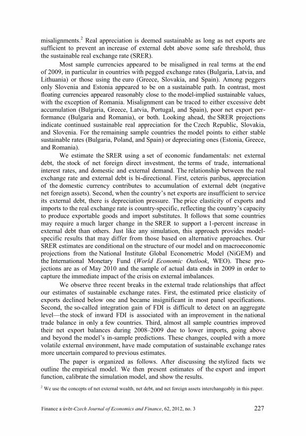
Until the Great Recession the NMS’s currencies were appreciating on aver-age by almost 3 percent annually during 1998–2009. Also, the currencies of Greece, Portugal, and Spain were appreciating in real terms by more than 1 percent annually (Figure 1, see the solid line). Depending on the exchange-rate regime, real apprecia-tion was effected through either nominal appreciation, higher domestic inflation, or a combination of the two.3 The real appreciation either could not be fully attributed to, or appeared to contradict, justifications such as the Balassa-Samuelson effect and the external wealth accumulation hypothesis of Lane and Milesi-Ferretti (2002). Regarding the former, nontradable goods sectors recorded as impressive productivity gains as tradable goods sectors (Mihaljek and Klau, 2004) and the empirical estimatesof the Balassa-Samuelson effect fall short of the observed real appreciation. Regard-ing the latter, the NMS currencies failed to depreciate in order to improve their trade balances in parallel to the rapid accumulation of net external debt. Moreover, the appreciation trend was simply too persistent to be the result of excessive devaluation at the start of the transition process as argued by Halpern and Wyplosz (1997). Further potential sources of trend appreciation—e.g. quality improvements in goods, pricing-to-market practices, country-specific effects of changing oil prices, and incomplete exchange rate pass-through—are discussed in Égert (2010).
Real appreciation in the NMS was also linked to massive inflows of foreign direct investment (FDI), which affected investors’ perceptions about the countries’ sustainable external balances (Schneider and Frey, 1985).4 In so far as FDI inflows contribute to export growth, capital inflows signal future net export gains consistent with sustainable foreign debt (negative net foreign assets) and real appreciation. The evidence on the relationship between FDI and the real exchange rate is mixed, however. On the one hand, in a cross-country setting, we observe a positive relation-ship between the stock of FDI and trade balance developments: trade balances improved in countries that accumulated more FDI than in those that accumulated less (Figure 2). On the other hand, over time, the increasing FDI-to-GDP ratio cor-responds to an improving trade balance in only four sample countries (the Czech Republic, Hungary, Poland, and Slovakia) and to either a worsening or unchanged trade balance in the others (Figure 1). These results are also consistent with anecdo-tal evidence that FDI inflows into the above four countries were directed mostly into tradable goods sectors (manufacturing and tourism) while in the rest of the sample these inflows were directed into nontradables (construction, banking, services, and so on). During 2002–2008 the shares of FDI flowing into tradable sectors in Bulgaria and Latvia were about one quarter of those in Poland or the Czech Republic (Figure 3).
3 The Baltic countries and Bulgaria retained the hard pegs established during the 1990s, while the Central European countries and later also Romania floated their currencies within the inflation-targeting frame-work. Slovenia, Cyprus, and Malta floated their currencies within a very narrow corridor against the euro and joined the euro area in 2007 and 2008, respectively. 4 The manifold effects of FDI inflows are difficult to disentangle empirically (see Bulíř and Šmídková, 2005, for a review). First, export capacity increased to the extent that FDI was directed into sectors producing tradables. Second, productivity spillovers positively affected aggregate productivity and real manufacturing output per worker grew. Third, FDI also stimulated imports as the FDI receiving sectors were incorporated into the production chain.
229 Finance a úvěr-Czech Journal of Economics and Finance, 62, 2012, no. 3
Figure 1 FDI, Real Effective Exchange Rate, External Debt, Net Exports
Bulgaria
-40
0
40
80
120
160
1998 2000 2002 2004 2006 2008
-30
-20
-10
0
10
FDI/GDP (l.s.)
REER (l.s.) NX/GDP (r.s.)
External debt (l.s.)
Czech Republic
-40
0
40
80
120
160
1998 2000 2002 2004 2006 2008
-30
-20
-10
0
10
Estonia
-40
0
40
80
120
160
1998 2000 2002 2004 2006 2008
-30
-20
-10
0
10Greece
-40
0
40
80
120
160
1998 2000 2002 2004 2006 2008
-30
-20
-10
0
10
Hungary
-40
0
40
80
120
160
1998 2000 2002 2004 2006 2008
-30
-20
-10
0
10Latvia
-40
0
40
80
120
160
1998 2000 2002 2004 2006 2008
-30
-20
-10
0
10
Lithuania
-40
0
40
80
120
160
1998 2000 2002 2004 2006 2008
-30
-20
-10
0
10
Portugal
-40
0
40
80
120
160
1998 2000 2002 2004 2006 2008
-30
-20
-10
0
10Romania
-40
0
40
80
120
160
1998 2000 2002 2004 2006 2008
-30
-20
-10
0
10
Slovakia
-40
0
40
80
120
160
1998 2000 2002 2004 2006 2008
-30
-20
-10
0
10Slovenia
-40
0
40
80
120
160
1998 2000 2002 2004 2006 2008
-30
-20
-10
0
10
Spain
-40
0
40
80
120
160
1998 2000 2002 2004 2006 2008
-30
-20
-10
0
10
Poland
-40
0
40
80
120
160
1998 2000 2002 2004 2006 2008
-30
-20
-10
0
10
Notes:
1. Foreign direct investment (FDI, ) is the stock of inward FDI as a ratio to GDP; in percent; left-hand scale. Source: International Financial Statistics, Balance of Payments Statistics.

Finance a úvěr-Czech Journal of Economics and Finance, 62, 2012, no. 3 230
2. Real effective exchange rate (REER, —) is the CPI-based, trade-weighted measure of external price competitiveness, 2000 = 0; in percent; left-hand scale. An upward-sloping line indicates real appreciation, that is, ceteris paribus, a loss of competitiveness. Source: IMF Information Notice System.
3. Net external debt (- - -) is the economy’s net foreign assets (assets minus liabilities) as a ratio to GDP; in percent; left-hand scale. Source: International Financial Statistics.
4. Net exports (NX, – –) is the balance on trade in goods (export minus imports) as a ratio to GDP; in percent; right-scale scale. Source: World Economic Outlook.
Figure 2 FDI and the Trade Balance in Goods, 1998–2008(change in percent of GDP)
b = 0.24R2 = 0.48
-10
-5
0
5
10
0 15 30 45Foreign direct investment
Tra
de b
ala
nce
Greece
Hungary
Malta
Slovakia
EstoniaCzech Republic
Poland
LithuaniaSlovenia
Romania
Portugal
Cyprus
Spain
Latvia
Notes: On the horizontal axis is the difference between the stock of net FDI-to-GDP ratio in 2001–2008 and 1996–1998. On the vertical axis is the difference between the average trade balance in goods as a ratio to GDP in 2001–2008 and 1996–1998. The simple linear regression implies that a 1-percentage-point increase in the stock of FDI corresponds to an improvement in the trade balance by about 0.2 percentage points.
Sources: IMF World Economic Outlook; authors’ calculations.
Figure 3 “Tradable FDI” as a Share of “Nontradable FDI,” 2002–2008
0.00
0.25
0.50
0.75
Poland CzechRepublic
Lithuania Hungary Romania Bulgaria Estonia Latvia
Notes: Tradable-sector FDI inflows are defined as those directed into manufacturing and tourism; nontradable-sector FDI is the residual. For Hungary, Poland, and Romania the series end in 2007. For Romania they start in 2004. The level of detail of the sectoral breakdown differed significantly across the sample.
Source: National central banks. We are indebted to Esteban Vesperoni for sharing these series.
All sample countries except Cyprus and Malta were net external debtors; they had negative net foreign assets (NFA) and external debt exploded in a few (Figure 1).While in 1998 only Hungary had external debt equivalent to more than 40 percent of GDP, by the end of the next decade the ratio exceeded 80 percent in Bulgaria, Estonia, Greece, Hungary, Latvia, Portugal, and Spain. What contributed to such accumulation of external liabilities? While in some countries NFA reflected cumula-tive FDI inflows (Estonia, Romania, and Slovakia), in others external liabilities grew
231 Finance a úvěr-Czech Journal of Economics and Finance, 62, 2012, no. 3
much faster than FDI (Greece, Latvia, Portugal, and also Hungary until 2005). Only in the Czech Republic and Slovenia was the NFA-to-GDP ratio below 40 percent and less than the FDI-to-GDP ratio in 2008.
3. The SRER Modeling Approach
The estimation of the SRER proceeds in two steps. First, in a panel of our sample countries, we estimate export and import equations. For the former we use the relative price of exports, external demand, and the FDI-to-GDP ratio, and for the latter we use the relative price of imports, domestic demand, and the FDI-to-GDP ratio.5 Second, we simulate the net external debt, FDI, and real exchange rate nexus of Šmídková, Barrel, and Holland (2002), imposing a steady-state ceiling on the stock of external debt. Our approach defines the SRER as a real exchange rate ensuring that net external debt is sustainable in the medium term. The SRER approach belongs to the equilibrium (fundamental) real exchange rate models (Williamson, 1994); furthermore, using the classification of Driver and Westaway (2005), it belongs to the medium-term structural methodologies that work with both stock and flow variables. To the extent that the SRER approach works with both the trade balance and NFA, it encompasses most of the fundamental real exchange rate models, in particular those based on flow variables, including some of the methodologies of the IMF Coordinating Group on Exchange Rate Issues (Lee et al., 2008). The SRER estimates hinge on two inputs: the values of the real exchange rate elasticity of external trade and the normatively chosen steady-state level of net external debt, both of which are estimates only.
The SRER literature has emphasized the role of FDI. In countries where FDI has been directed into tradable goods sectors, the resulting improvement in net exports has contributed to sustainable real appreciation. FDI is not homogeneous, and its impact on the economy, the trade balance, and real exchange rates depends on the capacity of the domestic economy to absorb the potential benefits of these inflows. On the one hand, the evidence supports the hypothesis that FDI has a positiveeffect on economic growth and productivity through the transfer of technology and skills and by augmenting the recipient’s domestic capital stock (Kose et al., 2006). On the other hand, FDI inflows seem to contribute to growth only in countries with a stock of human capital beyond a certain threshold or with well-developed financial markets and with sufficient provision of infrastructure (Borensztein, de Gregorio, and Lee, 1998). When such conditions are met, FDI contributes to economic growth by augmenting capital accumulation by “crowding-in” domestic investment.
The SRER calculation is built around empirically estimated trade equations with the usual fundamental variables while directly incorporating the impact of FDI (Šmídková, Barrell, and Holland, 2003). The current account balance is not restricted as NFA define the external equilibrium. The sustainable level of NFA is related to the country’s openness to trade as in Lee et al. (2008) and to the amount by which
5 The SRER approach is motivated by a dynamic model of a small, open economy, the external develop-ments of which are affected by FDI (Bulíř and Šmídková, 2005). FDI affects growth through two channels:first, through an increase in total investment (Holland and Pain, 1998) and, second, through interaction of the FDI’s more advanced technology with the host’s human capital (Borensztein et al., 1998, and Lim, 2001).

Finance a úvěr-Czech Journal of Economics and Finance, 62, 2012, no. 3 232
the actual debt deviates from its sustainable level; the more the discrepancy, the more the observed real exchange rate differs from the SRER.
Empirically, exports increase with foreign demand, improvement in the relativeprice of domestic goods (through either real depreciation or a terms-of-trade change), and the stock of FDI to approximate the integration gain:
11
23*
0m x
m
EP PX Y F
P P
(1)
where X denotes an export volume index; E is the US dollar nominal exchange rate vis-à-vis the domestic currency; Pm and Px are the effective prices of imports and exports, respectively (following the approach of NiGEM, the real exchange rate is defined in terms of the relative import price, which makes it convenient to represent the relative price of exports EPx/P as the product of the relative import price EPm/Pand the terms of trade Px/Pm—see Barrell, Holland, and Šmídková, 2002); P is the consumer price level; Y* is foreign demand; and F is the FDI-to-GDP ratio. Para-meters 1 through 3 all have nonnegative expected values.6
Demand for imports is driven by domestic activity, the real exchange rate, and FDI:
1
32
0mEP
M Y FP
(2)
where M denotes an import volume index and Y is domestic output. The parameter
1 has a negative expected value and the parameters 2 and 3 have positive
expected values. The stylized facts suggest that for some but not all countries we should observe that FDI improves net exports, i.e., 3 3 .
The trade balance, current-period external borrowing, and external-debt interest payments affect the level of net external debt, the sustainable level of which is determined by financial markets. We approximate the path of sustainable debt by considering the initial stock of debt, the country-specific sustainable debt target for the end of the simulation period, and three possible transition paths. The sustainable debt target is based on IMF estimates:
*0 , TD D D (3)
where D* denotes the sustainable path of net external debt (NFA in percent of GDP), and D0 and DT are the initial and target levels.
The SRER, C*, is then defined by solving equations (1)–(3):
1
1 1 23 32* * * * *
0 0 1 1(1 )x
m
PM C Y F X C Y F r D Y D Y
P
(4)
where M and X are the volume of real imports and exports, respectively, and r is the world real interest rate.
6 We also experimented with the exclusion of country-specific productivity relative to that of the euro area. However, we finally dropped productivity from the export equation as foreign demand and productivity turned out to be multicorrelated.

233 Finance a úvěr-Czech Journal of Economics and Finance, 62, 2012, no. 3
3.1 Trade Equations
The trade equations are estimated in a dynamic equilibrium correction model (ECM) using quarterly data over 1998–2009. The beginning of the sample is given by data availability (in particular with respect to the IMF estimates of the FDIstocks). The actual data cover the period up to 2009q3 or 2009q4 depending on the country under review, followed by the predictions up to 2014q4 that will be used to perform the simulations. As the variables in levels are nonstationary and our sample period of about one decade is too short for robust testing of the order of integration of the series and cointegration relationships, we specify the equations directly as an ECM, allowing for long-run relationships between the variables in levels and capturing the short-run dynamics. The cointegration tests are performed in the ECM. In addition, we perform system estimates imposing common elasticities across countries but allowing for country-specific terms:
*, 0, , 1 1 , 1 2 , 1 3 , 1Δ ln ln ln ln lni t i i t i t i t i tX A X RPX Y F
*4, , 5, , ,Δ ln Δ lni i t i i t i tRPX Y (5)
, 0, , 1 1 , 1 2 , 1 3 , 1Δ ln ln ln ln lni t i i t i t i t i tM B M RPM Y F
4, , 5, , ,Δ ln Δ lni i t i i t i tRPM Y u (6)
where 0 0exp( )A , 0 0expB , .m x
m
EP PRPX
P P
and mEPRPM
P
are the relative prices of exports and imports, respectively, the parameters λ and δcharacterize the speed of adjustment toward the long-run equilibrium, and ,i t and
,i tu are white noise disturbances.
Data consistency is crucial for the SRER calculations given the endogenous relationships among the variables, and we rely mostly on the global econometric model (NiGEM) and the IMF series (Table 1).7 The NiGEM series are quarterly, actual observations for the period 1998–2009 and projections for 2010–2014. The IMF’s International Financial Statistics NFA series are also quarterly, while the World Economic Outlook FDI series are annual and we use cubic intrapolation to increase the series frequency. The net external debt trajectory is a normative projection.
The panel approach involves a trade-off between country- and group-specific results. While the former tend to improve the short-run fit for the individual coun-tries, they complicate the long-run cross-country comparisons and capture transi-tional rather than long-run results—see Fic, Barrell, and Holland (2008). Basing the SRER estimates on the country-specific elasticities would mix estimates from the euro-area countries that are reasonably close to their steady state (say, Spain and
7 NiGEM is the large-scale quarterly macroeconomic model of the world economy created and maintained by the London-based National Institute of Economic and Social Research (http://www.niesr.ac.uk). Details of the model are available via the Internet: http://nimodel.niesr.ac.uk/.
Finance a úvěr-Czech Journal of Economics and Finance, 62, 2012, no. 3 234
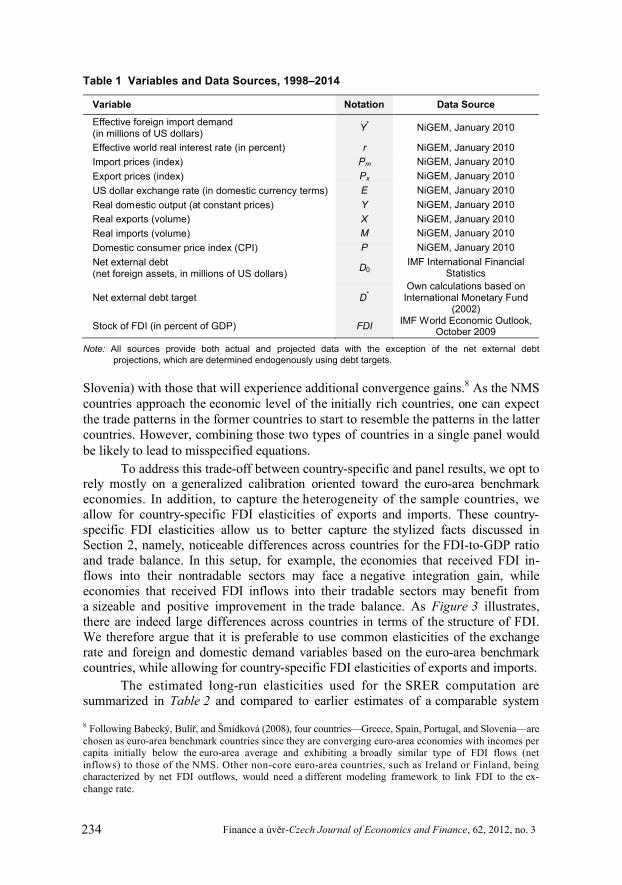
Table 1 Variables and Data Sources, 1998–2014
Variable Notation Data Source
Effective foreign import demand (in millions of US dollars)
Y* NiGEM, January 2010
Effective world real interest rate (in percent) r NiGEM, January 2010
Import prices (index) Pm NiGEM, January 2010
Export prices (index) Px NiGEM, January 2010
US dollar exchange rate (in domestic currency terms) E NiGEM, January 2010
Real domestic output (at constant prices) Y NiGEM, January 2010
Real exports (volume) X NiGEM, January 2010
Real imports (volume) M NiGEM, January 2010
Domestic consumer price index (CPI) P NiGEM, January 2010
Net external debt (net foreign assets, in millions of US dollars)
D0IMF International Financial
Statistics
Net external debt target D*Own calculations based on
International Monetary Fund (2002)
Stock of FDI (in percent of GDP) FDIIMF World Economic Outlook,
October 2009
Note: All sources provide both actual and projected data with the exception of the net external debt projections, which are determined endogenously using debt targets.
Slovenia) with those that will experience additional convergence gains.8 As the NMS countries approach the economic level of the initially rich countries, one can expect the trade patterns in the former countries to start to resemble the patterns in the latter countries. However, combining those two types of countries in a single panel would be likely to lead to misspecified equations.
To address this trade-off between country-specific and panel results, we opt to rely mostly on a generalized calibration oriented toward the euro-area benchmark economies. In addition, to capture the heterogeneity of the sample countries, we allow for country-specific FDI elasticities of exports and imports. These country-specific FDI elasticities allow us to better capture the stylized facts discussed in Section 2, namely, noticeable differences across countries for the FDI-to-GDP ratio and trade balance. In this setup, for example, the economies that received FDI in-flows into their nontradable sectors may face a negative integration gain, while economies that received FDI inflows into their tradable sectors may benefit from a sizeable and positive improvement in the trade balance. As Figure 3 illustrates, there are indeed large differences across countries in terms of the structure of FDI. We therefore argue that it is preferable to use common elasticities of the exchange rate and foreign and domestic demand variables based on the euro-area benchmark countries, while allowing for country-specific FDI elasticities of exports and imports.
The estimated long-run elasticities used for the SRER computation are summarized in Table 2 and compared to earlier estimates of a comparable system
8 Following Babecký, Bulíř, and Šmídková (2008), four countries—Greece, Spain, Portugal, and Slovenia—arechosen as euro-area benchmark countries since they are converging euro-area economies with incomes per capita initially below the euro-area average and exhibiting a broadly similar type of FDI flows (net inflows) to those of the NMS. Other non-core euro-area countries, such as Ireland or Finland, being characterized by net FDI outflows, would need a different modeling framework to link FDI to the ex-change rate.
235 Finance a úvěr-Czech Journal of Economics and Finance, 62, 2012, no. 3
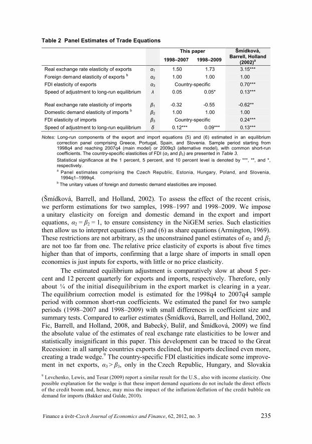
Table 2 Panel Estimates of Trade Equations
This paper Šmídková, Barrell, Holland
(2002)a1998–2007 1998–2009
Real exchange rate elasticity of exports α1 1.50 1.73 3.15***
Foreign demand elasticity of exports b α2 1.00 1.00 1.00
FDI elasticity of exports α3 Country-specific 0.70***
Speed of adjustment to long-run equilibrium λ 0.05 0.05* 0.13***
Real exchange rate elasticity of imports β1 -0.32 -0.55 -0.62**
Domestic demand elasticity of imports b β2 1.00 1.00 1.00
FDI elasticity of imports β3 Country-specific 0.24***
Speed of adjustment to long-run equilibrium δ 0.12*** 0.09*** 0.13***
Notes: Long-run components of the export and import equations (5) and (6) estimated in an equilibrium correction panel comprising Greece, Portugal, Spain, and Slovenia. Sample period starting from 1998q4 and reaching 2007q4 (main model) or 2009q3 (alternative model), with common short-run coefficients. The country-specific elasticities of FDI (α3 and β3) are presented in Table 3.
Statistical significance at the 1 percent, 5 percent, and 10 percent level is denoted by ***, **, and *, respectively.a
Panel estimates comprising the Czech Republic, Estonia, Hungary, Poland, and Slovenia, 1994q1–1999q4.
bThe unitary values of foreign and domestic demand elasticities are imposed.
(Šmídková, Barrell, and Holland, 2002). To assess the effect of the recent crisis, we perform estimations for two samples, 1998–1997 and 1998–2009. We impose a unitary elasticity on foreign and domestic demand in the export and import equations, α2 = β2 = 1, to ensure consistency in the NiGEM series. Such elasticities then allow us to interpret equations (5) and (6) as share equations (Armington, 1969). These restrictions are not arbitrary, as the unconstrained panel estimates of α2 and β2
are not too far from one. The relative price elasticity of exports is about five times higher than that of imports, confirming that a large share of imports in small open economies is just inputs for exports, with little or no price elasticity.
The estimated equilibrium adjustment is comparatively slow at about 5 per-cent and 12 percent quarterly for exports and imports, respectively. Therefore, only about ¼ of the initial disequilibrium in the export market is clearing in a year. The equilibrium correction model is estimated for the 1998q4 to 2007q4 sample period with common short-run coefficients. We estimated the panel for two sample periods (1998–2007 and 1998–2009) with small differences in coefficient size and summary tests. Compared to earlier estimates (Šmídková, Barrell, and Holland, 2002, Fic, Barrell, and Holland, 2008, and Babecký, Bulíř, and Šmídková, 2009) we find the absolute value of the estimates of real exchange rate elasticities to be lower and statistically insignificant in this paper. This development can be traced to the Great Recession: in all sample countries exports declined, but imports declined even more, creating a trade wedge.9 The country-specific FDI elasticities indicate some improve-ment in net exports, α3 > β3, only in the Czech Republic, Hungary, and Slovakia
9 Levchenko, Lewis, and Tesar (2009) report a similar result for the U.S., also with income elasticity. One possible explanation for the wedge is that these import demand equations do not include the direct effects of the credit boom and, hence, may miss the impact of the inflation/deflation of the credit bubble ondemand for imports (Bakker and Gulde, 2010).
Finance a úvěr-Czech Journal of Economics and Finance, 62, 2012, no. 3 236
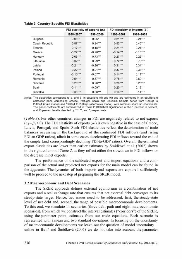
Table 3 Country-Specific FDI Elasticities
FDI elasticity of exports (α3) FDI elasticity of imports (β3)
1998–2007 1998–2009 1998–2007 1998–2009
Bulgaria 0.05** 0.05* 0.21*** 0.21***
Czech Republic 0.87*** 0.94*** 0.53*** 0.45***
Estonia 0.17*** 0.18*** 0.24*** 0.21***
Greece -0.22*** -0.20*** -0.14*** -0.16***
Hungary 0.66*** 0.73*** 0.27*** 0.23***
Lithuania 0.32** 0.29** 0.72*** 0.70***
Latvia -0.21*** -0.26*** 0.31*** 0.34***
Poland 0.22*** 0.21*** 0.37*** 0.38***
Portugal -0.10*** -0.07** 0.14*** 0.11***
Romania 0.54*** 0.57*** 0.78*** 0.69***
Slovenia 0.26*** 0.28*** 0.28*** 0.26***
Spain -0.11*** -0.09** 0.20*** 0.16***
Slovakia 0.35*** 0.38*** 0.16*** 0.14***
Notes: The elasticities correspond to α3 and β3 in equations (5) and (6) and are estimated in an equilibrium correction panel comprising Greece, Portugal, Spain, and Slovenia. Sample period from 1998q4 to 2007q4 (main model) and 1998q4 to 2009q3 (alternative model), with common short-run coefficients. The panel coefficients are summarized in Table 2. Statistical significance at the 1 percent, 5 percent, and 10 percent level is denoted by ***, **, and *, respectively.
(Table 3). For other countries, changes in FDI are negatively related to net exports (α3 – β3 < 0) The FDI elasticity of exports (α3) is even negative in the case of Greece, Latvia, Portugal, and Spain. Such FDI elasticities reflect the deterioration of trade balances occurring in the background of the continued FDI inflows (and risingFDI-to-GDP ratios), albeit in some cases decelerating FDI inflows toward the end of the sample (and correspondingly declining FDI-to-GDP ratios). Overall, the estimatedexport elasticities are lower than earlier estimates by Šmídková et al. (2002) shown in the right column of Table 2, as they reflect either the slowdown in FDI inflows or the decrease in net exports.
The performance of the calibrated export and import equations and a com-parison of the actual and predicted net exports for the main model can be found in the Appendix. The dynamics of both imports and exports are captured sufficiently well to proceed to the next step of preparing the SRER model.
3.2 Macroeconomic and Debt Scenarios
The SRER approach defines external equilibrium as a combination of net exports and a real exchange rate that ensures that net external debt converges to its steady-state target. Hence, two issues need to be addressed: first, the steady-state level of net debt and, second, the range of possible macroeconomic developments. To this end, we simulate 11 scenarios (three debt-path and eight macroeconomicscenarios), from which we construct the interval estimates (“corridors”) of the SRER, using the parameter point estimates from our trade equations. Each scenario is represented with a mean and two standard deviations. In focusing on the uncertainty of macroeconomic developments we leave out the question of model uncertainty—unlike in Bulíř and Šmídková (2005) we do not take into account the parameter
237 Finance a úvěr-Czech Journal of Economics and Finance, 62, 2012, no. 3
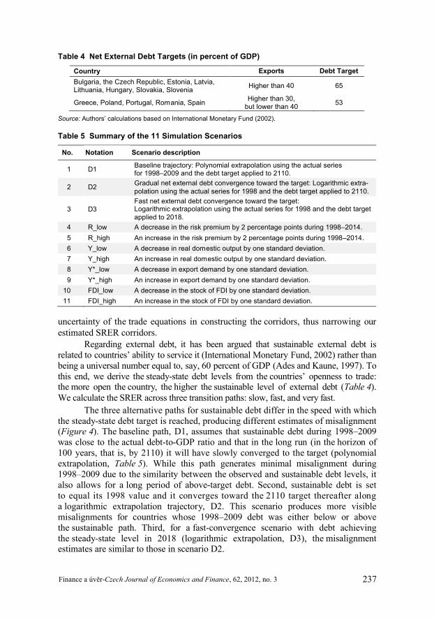
Table 4 Net External Debt Targets (in percent of GDP)
Country Exports Debt Target
Bulgaria, the Czech Republic, Estonia, Latvia, Lithuania, Hungary, Slovakia, Slovenia
Higher than 40 65
Greece, Poland, Portugal, Romania, Spain Higher than 30,
but lower than 4053
Source: Authors’ calculations based on International Monetary Fund (2002).
Table 5 Summary of the 11 Simulation Scenarios
No. Notation Scenario description
1 D1Baseline trajectory: Polynomial extrapolation using the actual series for 1998–2009 and the debt target applied to 2110.
2 D2Gradual net external debt convergence toward the target: Logarithmic extra-polation using the actual series for 1998 and the debt target applied to 2110.
3 D3Fast net external debt convergence toward the target: Logarithmic extrapolation using the actual series for 1998 and the debt target applied to 2018.
4 R_low A decrease in the risk premium by 2 percentage points during 1998–2014.
5 R_high An increase in the risk premium by 2 percentage points during 1998–2014.
6 Y_low A decrease in real domestic output by one standard deviation.
7 Y_high An increase in real domestic output by one standard deviation.
8 Y*_low A decrease in export demand by one standard deviation.
9 Y*_high An increase in export demand by one standard deviation.
10 FDI_low A decrease in the stock of FDI by one standard deviation.
11 FDI_high An increase in the stock of FDI by one standard deviation.
uncertainty of the trade equations in constructing the corridors, thus narrowing our estimated SRER corridors.
Regarding external debt, it has been argued that sustainable external debt is related to countries’ ability to service it (International Monetary Fund, 2002) rather than being a universal number equal to, say, 60 percent of GDP (Ades and Kaune, 1997). To this end, we derive the steady-state debt levels from the countries’ openness to trade: the more open the country, the higher the sustainable level of external debt (Table 4). We calculate the SRER across three transition paths: slow, fast, and very fast.
The three alternative paths for sustainable debt differ in the speed with which the steady-state debt target is reached, producing different estimates of misalignment (Figure 4). The baseline path, D1, assumes that sustainable debt during 1998–2009 was close to the actual debt-to-GDP ratio and that in the long run (in the horizon of 100 years, that is, by 2110) it will have slowly converged to the target (polynomial extrapolation, Table 5). While this path generates minimal misalignment during 1998–2009 due to the similarity between the observed and sustainable debt levels, it also allows for a long period of above-target debt. Second, sustainable debt is set to equal its 1998 value and it converges toward the 2110 target thereafter along a logarithmic extrapolation trajectory, D2. This scenario produces more visible misalignments for countries whose 1998–2009 debt was either below or above the sustainable path. Third, for a fast-convergence scenario with debt achieving the steady-state level in 2018 (logarithmic extrapolation, D3), the misalignment estimates are similar to those in scenario D2.
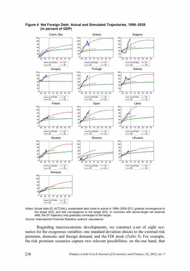
Finance a úvěr-Czech Journal of Economics and Finance, 62, 2012, no. 3 238
Figure 4 Net Foreign Debt: Actual and Simulated Trajectories, 1998–2039 (in percent of GDP)
0
20
40
60
80
100
120
00 05 10 15 20 25 30 35
D_ACTUAL D1
D2 D3
Czech_Rep
0
20
40
60
80
100
120
00 05 10 15 20 25 30 35
D_ACTUAL D1
D2 D3
Greece
0
20
40
60
80
100
120
00 05 10 15 20 25 30 35
D_ACTUAL D1
D2 D3
Bulgaria
0
20
40
60
80
100
120
00 05 10 15 20 25 30 35
D_ACTUAL D1D2 D3
Hungary
0
20
40
60
80
100
120
00 05 10 15 20 25 30 35
D_ACTUAL D1D2 D3
Portugal
0
20
40
60
80
100
120
00 05 10 15 20 25 30 35
D_ACTUAL D1D2 D3
Estonia
0
20
40
60
80
100
120
00 05 10 15 20 25 30 35
D_ACTUAL D1D2 D3
Poland
0
20
40
60
80
100
120
00 05 10 15 20 25 30 35
D_ACTUAL D1D2 D3
Spain
0
20
40
60
80
100
120
00 05 10 15 20 25 30 35
D_ACTUAL D1D2 D3
Latvia
0
20
40
60
80
100
120
00 05 10 15 20 25 30 35
D_ACTUAL D1D2 D3
Slovakia
0
20
40
60
80
100
120
00 05 10 15 20 25 30 35
D_ACTUAL D1D2 D3
Slovenia
0
20
40
60
80
100
120
00 05 10 15 20 25 30 35
D_ACTUAL D1D2 D3
Lithuania
0
20
40
60
80
100
120
00 05 10 15 20 25 30 35
D_ACTUAL D1D2 D3
Romania
Notes: Actual data (D_ACTUAL); sustainable debt close to actual in 1998–2009 (D1); gradual convergence to the target (D2); and fast convergence to the target (D3). In countries with above-target net external debt, the D1 trajectory only gradually converges to the target.
Source: International Financial Statistics; authors’ calculations
Regarding macroeconomic developments, we construct a set of eight sce-narios for the exogenous variables: one standard deviation shocks to the external risk premium, domestic and foreign demand, and the FDI stock (Table 5). For example, the risk premium scenarios capture two relevant possibilities: on the one hand, that
239 Finance a úvěr-Czech Journal of Economics and Finance, 62, 2012, no. 3
the adoption of the euro would be accompanied by a decrease in the risk premium (Schadler et al., 2005) and, on the other hand, that the 2009–2010 Greek debt crisis spills over into the NMS. These shocks are relatively large, as the corresponding standard deviations are equivalent to about 10 percent of the 2007 values. The com-puted SRER intervals are therefore quite robust, in particular capturing uncertainty related to the recent financial crisis through the scenarios of lower and higher risk premiums and reduced export demand.
4. Simulation Results
We report two types of simulation results, all performed in the EViews 7 package. First, we report estimates of currency misalignment for 1999–2009 using elasticities from the main model. The estimate range indicates real overvaluation//undervaluation if the interval is above/below the zero horizontal line. Second, we show the SRER projections for 2010–2014. Horizontal estimate ranges indicate a stable real exchange rate; downward/upward sloping ranges indicate real appre-ciation/depreciation.
4.1 Misalignment
Looking back, the floating exchange rates in the inflation-targeting countries were mostly close to their sustainable values, while the rates in the pegging countries were mostly overvalued, although with some exceptions. Our results are consistent with the common view that pegged currencies are more likely to be overvalued in real terms compared to floating ones (see Coudert and Couharde, 2009, and Dubas, 2009). To this end, in Figure 5 we report in the first column the inflation-targeting coun-tries (the Czech Republic, Hungary, Poland, Slovakia, and Romania), in the second the euro-area countries (Greece, Portugal, Spain, and Slovenia), and in the third those with hard pegs (Bulgaria, Estonia, Latvia, and Lithuania).10 The values for real mis-alignment in 2009 are shown in Table 7.
The inflation-targeting countries all had short-lived periods of either over- or undervaluation—the Czech Republic in 2007/2008, Hungary in the mid-2000s, Poland in 2001/2002, and Slovakia in 2009—but the currency misalignments disappeared quickly. Quantitatively, we estimate that these misalignments were about 10 percent or less. Despite fast accumulation of external liabilities and real appreciation of the national currencies, the actual real exchange rate remained close to the SRER, mainly on account of improvements in the trade balance. Slovakia shows an overvaluation of about 10–15 percent as the koruna was revalued prior to the adoption of the euro on January 1, 2009 and as Slovak inflation picked up relative to Germany and France.11 Romania, which floated its national currency only in 2005, was an exception in the subsample: the misalignment of the leu kept growing to almost 30 percent as the trade balance worsened and the real exchange rate continued to appreciate until 2008.
All three early euro-area countries (Greece, Portugal, and Spain) show signs of persistent overvaluation. Portugal and Spain narrowed their estimated misalign-
10 Slovakia joined the euro area in 2009, so we still include it among the inflation targeters.11 Bulíř and Hurník (2009) noted that a number of euro-area countries suffered from a sudden increase in inflation after euro adoption as pent-up inflationary pressures were released.

Finance a úvěr-Czech Journal of Economics and Finance, 62, 2012, no. 3 240
Figure 5 Real Exchange Rate Misalignment, 1999–2009(based on the panel estimates of the trade equations in Tables 2 and 3)
-.4
-.2
.0
.2
.4
00 02 04 06 08
Czech_Rep
-.4
-.2
.0
.2
.4
00 02 04 06 08
Greece
-.4
-.2
.0
.2
.4
00 02 04 06 08
Bulgaria
-.4
-.2
.0
.2
.4
00 02 04 06 08
Hungary
-.4
-.2
.0
.2
.4
00 02 04 06 08
Portugal
-.4
-.2
.0
.2
.4
00 02 04 06 08
Estonia
-.4
-.2
.0
.2
.4
00 02 04 06 08
Poland
-.4
-.2
.0
.2
.4
00 02 04 06 08
Spain
-.4
-.2
.0
.2
.4
00 02 04 06 08
Latvia
-.4
-.2
.0
.2
.4
00 02 04 06 08
Slovakia
-.4
-.2
.0
.2
.4
00 02 04 06 08
Slovenia
-.4
-.2
.0
.2
.4
00 02 04 06 08
Lithuania
-.4
-.2
.0
.2
.4
00 02 04 06 08
Romania
Notes: Values above/below the zero line indicate over/undervaluation of the national currency. Overvaluation is equivalent to excessive appreciation and, hence, a loss in external competitiveness. The middle line is the mean of the 11 scenarios described in the text; the upper and lower dashed lines show ±2 stand-ard deviations.
ments from 20 percent and 10 percent, respectively, to almost nil before the recentcrisis and a renewed widening in 2008–2009. Meanwhile, Greece’s currency appears to be overvalued throughout the sample period by 20–30 percent, with an increase to about 40 percent in 2009. In contrast, the estimated corridor for Slovenia’s currency is close to equilibrium, with relatively small appreciation vis-à-vis the SRER afterthe adoption of the euro in 2007. All four pegged currencies also appear to be over-valued, with Estonia and Lithuania only marginally such that the bottom of the cor-
241 Finance a úvěr-Czech Journal of Economics and Finance, 62, 2012, no. 3
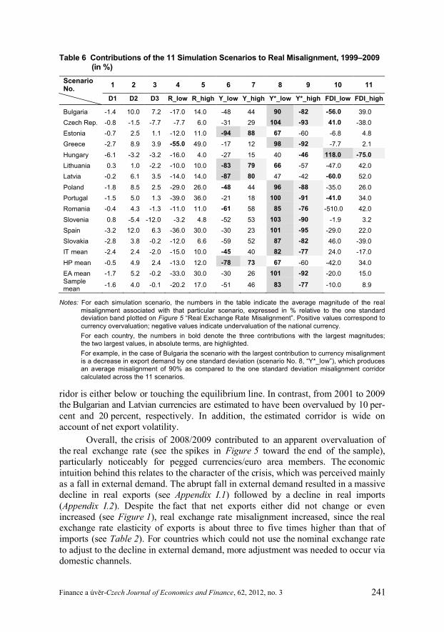
Table 6 Contributions of the 11 Simulation Scenarios to Real Misalignment, 1999–2009 (in %)
Scenario No.
1 2 3 4 5 6 7 8 9 10 11
D1 D2 D3 R_low R_high Y_low Y_high Y*_low Y*_high FDI_low FDI_high
Bulgaria -1.4 10.0 7.2 -17.0 14.0 -48 44 90 -82 -56.0 39.0
Czech Rep. -0.8 -1.5 -7.7 -7.7 6.0 -31 29 104 -93 41.0 -38.0
Estonia -0.7 2.5 1.1 -12.0 11.0 -94 88 67 -60 -6.8 4.8
Greece -2.7 8.9 3.9 -55.0 49.0 -17 12 98 -92 -7.7 2.1
Hungary -6.1 -3.2 -3.2 -16.0 4.0 -27 15 40 -46 118.0 -75.0
Lithuania 0.3 1.0 -2.2 -10.0 10.0 -83 79 66 -57 -47.0 42.0
Latvia -0.2 6.1 3.5 -14.0 14.0 -87 80 47 -42 -60.0 52.0
Poland -1.8 8.5 2.5 -29.0 26.0 -48 44 96 -88 -35.0 26.0
Portugal -1.5 5.0 1.3 -39.0 36.0 -21 18 100 -91 -41.0 34.0
Romania -0.4 4.3 -1.3 -11.0 11.0 -61 58 85 -76 -510.0 42.0
Slovenia 0.8 -5.4 -12.0 -3.2 4.8 -52 53 103 -90 -1.9 3.2
Spain -3.2 12.0 6.3 -36.0 30.0 -30 23 101 -95 -29.0 22.0
Slovakia -2.8 3.8 -0.2 -12.0 6.6 -59 52 87 -82 46.0 -39.0
IT mean -2.4 2.4 -2.0 -15.0 10.0 -45 40 82 -77 24.0 -17.0
HP mean -0.5 4.9 2.4 -13.0 12.0 -78 73 67 -60 -42.0 34.0
EA mean -1.7 5.2 -0.2 -33.0 30.0 -30 26 101 -92 -20.0 15.0Sample mean
-1.6 4.0 -0.1 -20.2 17.0 -51 46 83 -77 -10.0 8.9
Notes: For each simulation scenario, the numbers in the table indicate the average magnitude of the real misalignment associated with that particular scenario, expressed in % relative to the one standard deviation band plotted on Figure 5 “Real Exchange Rate Misalignment”. Positive values correspond to currency overvaluation; negative values indicate undervaluation of the national currency.
For each country, the numbers in bold denote the three contributions with the largest magnitudes; the two largest values, in absolute terms, are highlighted.
For example, in the case of Bulgaria the scenario with the largest contribution to currency misalignment is a decrease in export demand by one standard deviation (scenario No. 8, “Y*_low”), which produces an average misalignment of 90% as compared to the one standard deviation misalignment corridor calculated across the 11 scenarios.
ridor is either below or touching the equilibrium line. In contrast, from 2001 to 2009 the Bulgarian and Latvian currencies are estimated to have been overvalued by 10 per-cent and 20 percent, respectively. In addition, the estimated corridor is wide on account of net export volatility.
Overall, the crisis of 2008/2009 contributed to an apparent overvaluation of the real exchange rate (see the spikes in Figure 5 toward the end of the sample), particularly noticeably for pegged currencies/euro area members. The economicintuition behind this relates to the character of the crisis, which was perceived mainly as a fall in external demand. The abrupt fall in external demand resulted in a massive decline in real exports (see Appendix I.1) followed by a decline in real imports (Appendix I.2). Despite the fact that net exports either did not change or even increased (see Figure 1), real exchange rate misalignment increased, since the real exchange rate elasticity of exports is about three to five times higher than that of imports (see Table 2). For countries which could not use the nominal exchange rate to adjust to the decline in external demand, more adjustment was needed to occur via domestic channels.
Finance a úvěr-Czech Journal of Economics and Finance, 62, 2012, no. 3 242
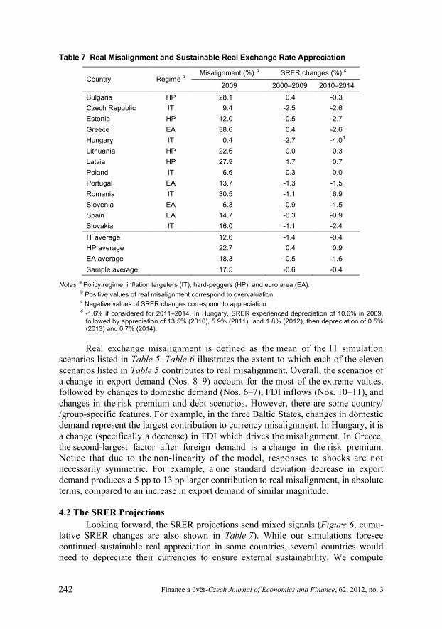
Table 7 Real Misalignment and Sustainable Real Exchange Rate Appreciation
Country Regime aMisalignment (%) b SRER changes (%) c
2009 2000–2009 2010–2014
Bulgaria HP 28.1 0.4 -0.3
Czech Republic IT 9.4 -2.5 -2.6
Estonia HP 12.0 -0.5 2.7
Greece EA 38.6 0.4 -2.6
Hungary IT 0.4 -2.7 -4.0d
Lithuania HP 22.6 0.0 0.3
Latvia HP 27.9 1.7 0.7
Poland IT 6.6 0.3 0.0
Portugal EA 13.7 -1.3 -1.5
Romania IT 30.5 -1.1 6.9
Slovenia EA 6.3 -0.9 -1.5
Spain EA 14.7 -0.3 -0.9
Slovakia IT 16.0 -1.1 -2.4
IT average 12.6 -1.4 -0.4
HP average 22.7 0.4 0.9
EA average 18.3 -0.5 -1.6
Sample average 17.5 -0.6 -0.4
Notes:a
Policy regime: inflation targeters (IT), hard-peggers (HP), and euro area (EA).b
Positive values of real misalignment correspond to overvaluation.c
Negative values of SRER changes correspond to appreciation.d
-1.6% if considered for 2011–2014. In Hungary, SRER experienced depreciation of 10.6% in 2009, followed by appreciation of 13.5% (2010), 5.9% (2011), and 1.8% (2012), then depreciation of 0.5% (2013) and 0.7% (2014).
Real exchange misalignment is defined as the mean of the 11 simulationscenarios listed in Table 5. Table 6 illustrates the extent to which each of the eleven scenarios listed in Table 5 contributes to real misalignment. Overall, the scenarios of a change in export demand (Nos. 8–9) account for the most of the extreme values, followed by changes to domestic demand (Nos. 6–7), FDI inflows (Nos. 10–11), and changes in the risk premium and debt scenarios. However, there are some country//group-specific features. For example, in the three Baltic States, changes in domestic demand represent the largest contribution to currency misalignment. In Hungary, it is a change (specifically a decrease) in FDI which drives the misalignment. In Greece, the second-largest factor after foreign demand is a change in the risk premium. Notice that due to the non-linearity of the model, responses to shocks are notnecessarily symmetric. For example, a one standard deviation decrease in export demand produces a 5 pp to 13 pp larger contribution to real misalignment, in absolute terms, compared to an increase in export demand of similar magnitude.
4.2 The SRER Projections
Looking forward, the SRER projections send mixed signals (Figure 6; cumu-lative SRER changes are also shown in Table 7). While our simulations foresee continued sustainable real appreciation in some countries, several countries would need to depreciate their currencies to ensure external sustainability. We compute
243 Finance a úvěr-Czech Journal of Economics and Finance, 62, 2012, no. 3
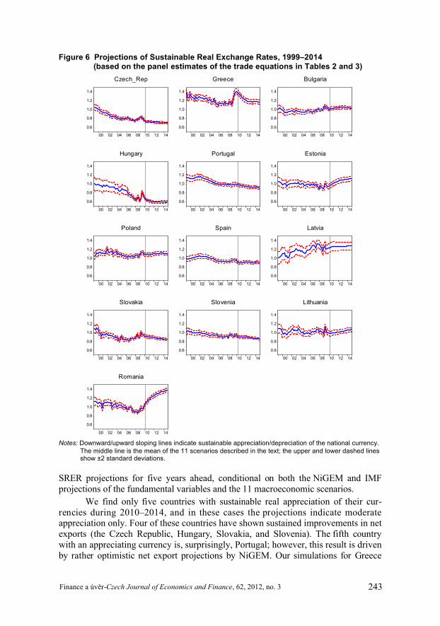
Figure 6 Projections of Sustainable Real Exchange Rates, 1999–2014(based on the panel estimates of the trade equations in Tables 2 and 3)
0.6
0.8
1.0
1.2
1.4
00 02 04 06 08 10 12 14
Czech_Rep
0.6
0.8
1.0
1.2
1.4
00 02 04 06 08 10 12 14
Greece
0.6
0.8
1.0
1.2
1.4
00 02 04 06 08 10 12 14
Bulgaria
0.6
0.8
1.0
1.2
1.4
00 02 04 06 08 10 12 14
Hungary
0.6
0.8
1.0
1.2
1.4
00 02 04 06 08 10 12 14
Portugal
0.6
0.8
1.0
1.2
1.4
00 02 04 06 08 10 12 14
Estonia
0.6
0.8
1.0
1.2
1.4
00 02 04 06 08 10 12 14
Poland
0.6
0.8
1.0
1.2
1.4
00 02 04 06 08 10 12 14
Spain
0.6
0.8
1.0
1.2
1.4
00 02 04 06 08 10 12 14
Latvia
0.6
0.8
1.0
1.2
1.4
00 02 04 06 08 10 12 14
Slovakia
0.6
0.8
1.0
1.2
1.4
00 02 04 06 08 10 12 14
Slovenia
0.6
0.8
1.0
1.2
1.4
00 02 04 06 08 10 12 14
Lithuania
0.6
0.8
1.0
1.2
1.4
00 02 04 06 08 10 12 14
Romania
Notes: Downward/upward sloping lines indicate sustainable appreciation/depreciation of the national currency. The middle line is the mean of the 11 scenarios described in the text; the upper and lower dashed lines show ±2 standard deviations.
SRER projections for five years ahead, conditional on both the NiGEM and IMF projections of the fundamental variables and the 11 macroeconomic scenarios.
We find only five countries with sustainable real appreciation of their cur-rencies during 2010–2014, and in these cases the projections indicate moderate appreciation only. Four of these countries have shown sustained improvements in net exports (the Czech Republic, Hungary, Slovakia, and Slovenia). The fifth country with an appreciating currency is, surprisingly, Portugal; however, this result is driven by rather optimistic net export projections by NiGEM. Our simulations for Greece
Finance a úvěr-Czech Journal of Economics and Finance, 62, 2012, no. 3 244
project some real appreciation in 2010–2012; however, the end-of-sample SRER level is depreciated relative to 2007. It is important to note that a country could be characterized by both an overvalued currency (i.e., a positive misalignment) and sus-tainable appreciation foreseen in the medium term. The reason is that the historical misalignment is not informative about the future SRER trajectory. If a currency is overvalued in real terms, it could depreciate, followed by subsequent SRER apprecia-tion.
The simulations point to stable SRERs in three countries (Poland, Spain, and Latvia) and depreciating SRERs in the rest (Bulgaria, Estonia, Lithuania, and Romania). Most notable is the depreciation required to achieve sustainable debt in Romania—some 30–40 percent relative to 2009. These simulations are conditional on the NiGEM projections for the individual countries, and these projections may change materially: for example, in January 2010 the growth, export, and import projections for Estonia changed so much that the direction of the sustainable ex-change rate path changed.
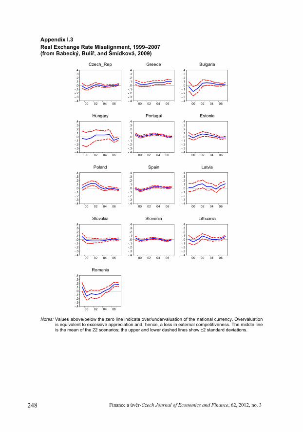
4.3 Comparisons with the Pre-Crisis Results
We compare our estimates of SRER misalignment and projections with two sets of our own estimates based on the pre-crisis data. First, the quarterly SRER estimates from Babecký, Bulíř, and Šmídková (2008) based on the trade elasticities from Barrell et al. (2002) are considered. Second, the annual SRER estimates based on Babecký, Bulíř, and Šmídková (2009) are also utilized. We can therefore trace the impact of the recent crisis on the SRER estimates through two channels. First, the projections for macroeconomic variables from NiGEM and FDI flows from WEO changed dramatically during the crisis. Second, the present SRER estimates use dif-ferent calibrations based on alternative trade equations. Moreover, the former paper covers only the Czech Republic, Greece, Hungary, Poland, Portugal, Slovakia, Slovenia, and Spain, while the latter adds Bulgaria, Estonia, Latvia, Lithuania, and Romania. For illustration of the impact of these differences, the previous estimates (from Babecký, Bulíř, and Šmídková, 2009) are shown in Appendix I.3 (real exchange rate misalignment) and Appendix I.4 (SRER projections).
While in a few countries (the Czech Republic and Slovenia) the misalignment estimates are practically indistinguishable from one another, in most countries the mean estimate shifted upward in the aftermath of the crisis, keeping the slope of the path of the misalignment estimate unchanged. The shift was negligible for Estonia, Poland, and Slovakia; however, it was sizable for Greece, Latvia, and Romania. For example, the annual-series simulations in Babecký, Bulíř, andŠmídková (2009) estimated that Greece’s currency may be overvalued by 10 percent at most, but the current estimate suggests overvaluation close to 30 percent.
We find a pronounced impact of the Great Recession on trade and net external debt in our 2010–2014 SRER projections. To recapitulate, in this paper we assess the impact of the Great Recession by estimating the elasticities for two samples, 1998–2007 and 1998–2009. As illustrated in Tables 2 and 3, the estimated elasticities are fairly similar across periods. Thus, the main effect of the recent crisis on real exchange rate misalignment and SRER projections was due to changes in the under-lying macroeconomic variables rather than the coefficients of the model. While in
245 Finance a úvěr-Czech Journal of Economics and Finance, 62, 2012, no. 3
the earlier papers’ simulations we found either appreciating or stable SRERs in our sample countries (see Figure 4 in Babecký, Bulíř, and Šmídková, 2008, or Figure V.2 in Babecký, Bulíř, and Šmídková, 2009), in this paper we find that a number of countries will require real depreciation to stabilize their external position. These changes are particularly pronounced for Bulgaria, Estonia, Greece, and Romania. In contrast, countries with healthy net trade balances (the Czech Republic, Hungary, Slovakia, and Slovenia) seem unaffected by the recent developments.
5. Conclusions
We simulate sustainable real exchange rates using a set of economic funda-mentals and find that the Great Recession had a profound impact on our estimates of real exchange rate misalignments and SRER projections. We find that after the crisis, the so-called integration gain of FDI inflows was limited to the Czech Republic, Hungary, and Slovakia. The price elasticity of exports and imports declined, be-coming insignificant in most specifications. A weakening of the relative-price-equilibrating mechanism affects the SRER—the lower the relative price elasticities, the more the real exchange rate must depreciate to support the debt service on an existing stock of external liabilities. Our estimates of the SRER are conditional on the structure of our model and on macroeconomic projections from the National Institute Global Econometric Model and the IMF (World Economic Outlook).
We find, first, that real misalignments in countries with mostly pegged exchange rates and with excessive external liabilities widened relative to earlier estimates of the SRER. In contrast, countries with flexible exchange rates seem to be closer to their fundamental equilibria; however, even their currencies appeared overvalued at the end of 2009. Looking ahead, countries with balanced net trade positions are expected to continue to appreciate during 2010–2014; still, several currencies are likely to require real depreciation to maintain sustainable net external debt. As most of the latter countries either are members of the euro area or have their currencies pegged to the euro, real depreciation will require a decrease of either domestic prices or external debt. Our estimates of the sustainable real exchange rates do not explicitly account for the structure of FDI and thus the differences in the results could also be due to the extent to which FDI inflows are divided between the tradable and non-tradable sectors of the economy. This could be an avenue for future research.

Finance a úvěr-Czech Journal of Economics and Finance, 62, 2012, no. 3 246
APPENDIX
Appendix I.1
Real Exports, 1998–2009, Actual (—) versus Estimated (- - -) Values
200,000
300,000
400,000
500,000
600,000
700,000
800,000
900,000
98 00 02 04 06 08
Czech_Rep
6
7
8
9
10
11
12
13
98 00 02 04 06 08
Greece
2
3
4
5
6
7
8
98 00 02 04 06 08
Bulgaria
1,000,000
2,000,000
3,000,000
4,000,000
5,000,000
6,000,000
7,000,000
98 00 02 04 06 08
Hungary
7
8
9
10
11
12
13
14
98 00 02 04 06 08
Portugal
12,000
16,000
20,000
24,000
28,000
32,000
36,000
40,000
98 00 02 04 06 08
Estonia
30,000
40,000
50,000
60,000
70,000
80,000
90,000
100,000
110,000
98 00 02 04 06 08
Poland
35
40
45
50
55
60
65
70
98 00 02 04 06 08
Spain
400
500
600
700
800
900
1,000
1,100
98 00 02 04 06 08
Latvia
2
4
6
8
10
12
14
98 00 02 04 06 08
Slovakia
2.0
2.5
3.0
3.5
4.0
4.5
5.0
98 00 02 04 06 08
Slovenia
4,000
6,000
8,000
10,000
12,000
14,000
98 00 02 04 06 08
Lithuania
4
6
8
10
12
14
16
18
98 00 02 04 06 08
Romania
Notes: Actual values show export volumes (XVOL). Estimated values are based on the main model, which uses estimates of demand and price elasticities on 1998q4–2007q4, country-specific FDI elasticities, and constant terms calibrated on 1998q4–2009q4.

247 Finance a úvěr-Czech Journal of Economics and Finance, 62, 2012, no. 3
Appendix I.2
Real Imports, 1998–2009, Actual (—) versus Estimated (- - -) Values
200,000
300,000
400,000
500,000
600,000
700,000
800,000
900,000
98 00 02 04 06 08
Czech_Rep
10
11
12
13
14
15
16
17
98 00 02 04 06 08
Greece
23456789
1011
98 00 02 04 06 08
Bulgaria
1,600,0002,000,0002,400,0002,800,0003,200,0003,600,0004,000,0004,400,0004,800,0005,200,0005,600,000
98 00 02 04 06 08
Hungary
11
12
13
14
15
16
17
98 00 02 04 06 08
Portugal
15,000
20,000
25,000
30,000
35,000
40,000
45,000
50,000
98 00 02 04 06 08
Estonia
40,00050,00060,00070,00080,00090,000
100,000110,000120,000130,000
98 00 02 04 06 08
Poland
40
50
60
70
80
90
98 00 02 04 06 08
Spain
400
600
800
1,000
1,200
1,400
1,600
98 00 02 04 06 08
Latvia
5
6
7
8
9
10
11
12
13
98 00 02 04 06 08
Slovakia
2.0
2.5
3.0
3.5
4.0
4.5
5.0
5.5
98 00 02 04 06 08
Slovenia
4,000
6,000
8,000
10,000
12,000
14,000
16,000
18,000
98 00 02 04 06 08
Lithuania
5
10
15
20
25
30
35
98 00 02 04 06 08
Romania
Notes: Actual values show export volumes (XVOL). Estimated values are based on the main model, which uses estimates of demand and price elasticities on 1998q4–2007q4, country-specific FDI elasticities, and constant terms calibrated on 1998q4–2009q4.
Finance a úvěr-Czech Journal of Economics and Finance, 62, 2012, no. 3 248
Appendix I.3
Real Exchange Rate Misalignment, 1999–2007 (from Babecký, Bulíř, and Šmídková, 2009)
-.4-.3-.2-.1.0.1.2.3.4
00 02 04 06
Czech_Rep
-.4-.3-.2-.1.0.1.2.3.4
00 02 04 06
Greece
-.4-.3-.2-.1.0.1.2.3.4
00 02 04 06
Bulgaria
-.4-.3-.2-.1.0.1.2.3.4
00 02 04 06
Hungary
-.4-.3-.2-.1.0.1.2.3.4
00 02 04 06
Portugal
-.4-.3-.2-.1.0.1.2.3.4
00 02 04 06
Estonia
-.4-.3-.2-.1.0.1.2.3.4
00 02 04 06
Poland
-.4-.3-.2-.1.0.1.2.3.4
00 02 04 06
Spain
-.4-.3-.2-.1.0.1.2.3.4
00 02 04 06
Latvia
-.4-.3-.2-.1.0.1.2.3.4
00 02 04 06
Slovakia
-.4-.3-.2-.1.0.1.2.3.4
00 02 04 06
Slovenia
-.4-.3-.2-.1.0.1.2.3.4
00 02 04 06
Lithuania
-.4-.3-.2-.1.0.1.2.3.4
00 02 04 06
Romania
Notes: Values above/below the zero line indicate over/undervaluation of the national currency. Overvaluation is equivalent to excessive appreciation and, hence, a loss in external competitiveness. The middle line is the mean of the 22 scenarios; the upper and lower dashed lines show ±2 standard deviations.
249 Finance a úvěr-Czech Journal of Economics and Finance, 62, 2012, no. 3
Appendix I.4
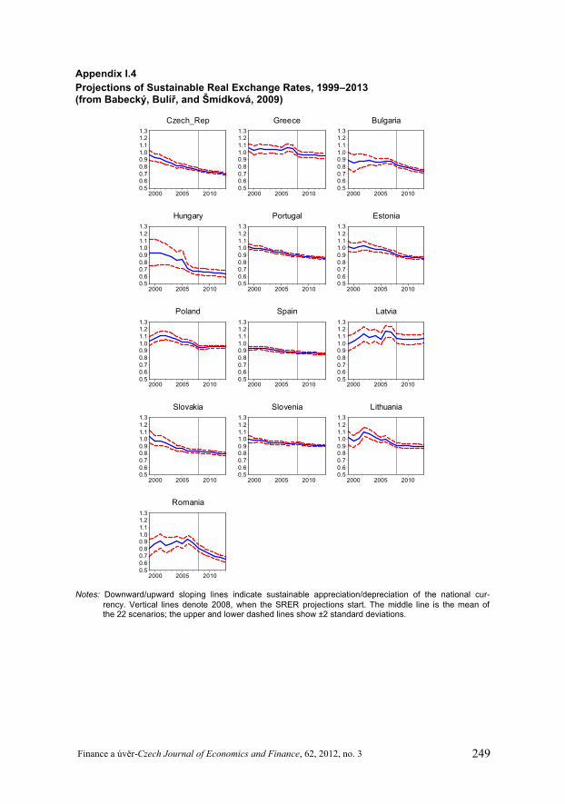
Projections of Sustainable Real Exchange Rates, 1999–2013(from Babecký, Bulíř, and Šmídková, 2009)
0.50.60.70.80.91.01.11.21.3
2000 2005 2010
Czech_Rep
0.50.60.70.80.91.01.11.21.3
2000 2005 2010
Greece
0.50.60.70.80.91.01.11.21.3
2000 2005 2010
Bulgaria
0.50.60.70.80.91.01.11.21.3
2000 2005 2010
Hungary
0.50.60.70.80.91.01.11.21.3
2000 2005 2010
Portugal
0.50.60.70.80.91.01.11.21.3
2000 2005 2010
Estonia
0.50.60.70.80.91.01.11.21.3
2000 2005 2010
Poland
0.50.60.70.80.91.01.11.21.3
2000 2005 2010
Spain
0.50.60.70.80.91.01.11.21.3
2000 2005 2010
Latvia
0.50.60.70.80.91.01.11.21.3
2000 2005 2010
Slovakia
0.50.60.70.80.91.01.11.21.3
2000 2005 2010
Slovenia
0.50.60.70.80.91.01.11.21.3
2000 2005 2010
Lithuania
0.50.60.70.80.91.01.11.21.3
2000 2005 2010
Romania
Notes: Downward/upward sloping lines indicate sustainable appreciation/depreciation of the national cur-rency. Vertical lines denote 2008, when the SRER projections start. The middle line is the mean of the 22 scenarios; the upper and lower dashed lines show ±2 standard deviations.
Finance a úvěr-Czech Journal of Economics and Finance, 62, 2012, no. 3 250
REFERENCES
Ades A, Kaune F (1997): A New Measure of Current Account Sustainability for Developing Countries. Goldman-Sachs Emerging Markets Economic Research. Goldman-Sachs, New-York.
Armington PS (1969): A Theory of Demand for Products Distinguished by Place of Production. IMF Staff Papers, 16(1):159–178.
Babecký J, Bulíř A, Šmídková K (2008): Sustainable Real Exchange Rates when Trade Winds Are Plentiful. National Institute Economic Review, 204:98–107.
Babecký J, Bulíř A, Šmídková K (2009): Sustainable Real Exchange Rates in the New EU Member States: Is FDI a Mixed Blessing? European Economy Economic Papers, no. 368.
Bakker BB, Gulde AM (2010): The Credit Boom in the EU New Member States: Bad Luck or Bad Policies? IMF Working Paper, no. 10/130.
Barrell R, Holland D, Jakab ZM, Kovács MA, Šmídková K, Sepp U, Čufer U (2002): An Econo-metric Macro-model of Transition: Policy Choices in the Pre-Accession Period. In: Modelling Economies in Transition—proceedings of AMFET 2001 Conference, Krag (Poland). Absolwent, Lodz.
Barrell R, Holland D, Šmídková K (2002): An Empirical Analysis of Monetary Policy Choices in the Pre-EMU Period. NIESR Discussion Paper, no. 204.
Borensztein E, Gregorio J de, Lee JW (1998): How Does Foreign Direct Investment Affect Economic Growth? Journal of International Economics, 45(1):115–135.
Bulíř A, Hurník J (2009): Inflation Convergence in the Euro Area: Just Another Gimmick? Journal of Financial Economic Policy, 1(4):355–369.
Bulíř A, Šmídková K (2005): Sustainable Real Exchange Rates in the New Accession Countries: What Have We Learned from the Forerunners? Economic Systems, 29(2):163–186.
Bulíř A, Šmídková K (2007): Fast Sailing Toward the Euro: Dangers of the Lee Shore. In: Batini N (Ed): Monetary Policy in Emerging Markets and Other Developing Countries. Nova Science Publishers, New York, pp. 67–92.
Coricelli F, Maurel M (2010): Growth and Crisis in Transition: A Comparative Perspective, Documents de travail du Centre d’Economie de la Sorbonne, no. 2010/20.
Coudert V, Couharde C (2009): Currency Misalignments and Exchange Rate Regimes in Emerging and Developing Countries. Review of International Economics, 17(1):121–136.
Driver R, Westaway PF (2005): Concepts of Equilibrium Exchange Rates. Bank of England Working Paper, no. 247.
Dubas JM (2009): The Importance of the Exchange Rate Regime in Limiting Misalignment. World Development, 37(10):1612–1622.
Égert B (2010): Catching-up and Inflation in Europe: Balassa-Samuelson, Engel’s Law and Other Culprits. OECD Economics Department Working Paper, no. 792.
Fic T, Barrell R, Holland D (2008): Entry Rates and the Risks of Misalignment in the EU8. Journal of Policy Modeling, 30(5):761–774.
Furceri D, Zdzienicka A (2011): The Real Effect of Financial Crises in the European Transition Economies. Economics of Transition, 19(1):1–25.
Halpern L, Wyplosz C (1997): Equilibrium Exchange Rates in Transition Economies. IMF Staff Papers, 44(4):430–461.
International Monetary Fund (2002): Assessing Sustainability. available at: http://www.imf.org/external/np/pdr/sus/2002/eng/052802.htm.
International Monetary Fund (2009): Greece: 2009 Article IV Consultation—Staff Report. available at: http://www.imf.org/external/pubs/ft/scr/2009/cr09244.pdf.
251 Finance a úvěr-Czech Journal of Economics and Finance, 62, 2012, no. 3
Keppel C, Wörz J (2010): The Impact of the Global Recession in Europe: The Role of International Trade. In: Backé P, Gnan E, Hartmann P (Eds): Contagion and Spillovers: New Insights from the Crisis. SUERF Studies (Vienna), no. 2010/5, pp. 115–140.
Kose MA, Prasad E, Rogoff K, Wei SJ (2006): Financial Globalization: A Reappraisal. IMF Working Paper, no. 06/189.
Lane PR, Milesi-Ferretti GM (2002): External Wealth, the Trade Balance, and the Real Exchange Rate. European Economic Review, 46(6):1049–1071.
Lee J, Milesi-Ferretti GM, Ostry J, Prati A, Ricci L (2008): Exchange Rate Assessments: CGER Methodologie. IMF Occasional Paper, no. 261.
Levchenko AA, Lewis L, Tesar LL (2009): The Collapse of International Trade During the 2008––2009 Crisis: In: Search of the Smoking Gun. Gerald R Ford School of Public Policy Discussion Paper, no. 592.
Lim EG (2001): Determinants of, and the Relation Between, Foreign Direct Investment and Growth: A Summary of the Recent Literature. IMF Working Paper, no. 01/175.
Mihaljek D, Klau M (2004): The Balassa-Samuelson Effect in Central Europe: A Disaggregated Analysis. Comparative Economic Studies, 46(1):63–94.
Schadler S, Drummond P, Kuijs L, Murgasova Z, Elkan R van (2005): Adopting the Euro in Central Europe—Challenges of the Next Step in European Integration. IMF Occasional Paper, no. 234.
Schneider F, Frey BS (1985): Economic and Political Determinants of Foreign Direct Investment. World Development, 13(2):161–175.
Šmídková K, Barrell R, Holland D (2002): Estimates of FRERs for the Five EU Accession Countries. CNB Working Paper, no. 3/2002.
Williamson J (1994): Estimating Equilibrium Exchange Rates. Institute for International Economics, Washington, DC.