Home Value and Homeownership Rates: Recession and Post-Recession Comparisons
16
American Community Survey Briefs U.S. Department of Commerce Economics and Statistics Administration U.S. CENSUS BUREAU census.gov Home Value and Homeownership Rates: Recession and Post-Reces sion Comparisons From 2007–2009 to 2010–2012 INTRODUCTION This report examines the differences in the median home value and homeownership rate across differ- ent geographies during and after the recession of 2007 through 2009. The data used in this report are from a 3-year period roughly encompassing part of the 2007–2009 recession and the 3 years following the recent recession 1 (2010 through 2012) collected in the American Community Survey (ACS). Using the 3-year ACS data enables us to look at geographies with smaller populations, 20,000 or more, than the geog- raphies available from the 1-year data. This report will focus on those changes at the nation, state, county, metropolitan area, and place (city) level. For the purpose of this report, areas with populations of 20,000 to 65,000 will be referred to as smaller cities or counties. The 50 least populous of the smaller cities or counties will be referred to as the least populous cities or counties. Since the latest publication of the American Community Survey Brief, “Property Value: 2008 and 2009,” which looked at median home value and the percent change in median home value for Metropoli- tan Statistical Areas, the recession in the United States has ended. Subsequently, metropolitan areas saw an increase in renter occupied housing units. 2 The United States experienced a significant decrease in median home value (–$17,300) as well as homeownership rate (–1.7) from 2007–2009 to 2010–2012. 1 The recent recession started in December 2007 and ended in June 2009 according to the National Bureau of Economic Research, Inc., 1050 Massachusetts Ave., Cambridge, MA, <www.nber.org/cycles /cyclesmain.html>. 2 See “Rental Housing Market Condition Measures: A Comparison of U.S. Metropolitan Areas From 2009 to 2011” by Christine Flanagan and Mary Schwartz. OWNER HOUSING MARKET CONDITION MEASURES Home Value As Figure 1 shows, the median home value in current dollars, based on decennial census data, rose slowly from 1940 to 1970. After that, the median home value rose steadily . By 2000, it had increased by more than seven times the median home value in 1970. How- ever, the housing bubble was followed by a housing crash and the recession. Figure 2, based on ACS data, which replaced the decennial long form, shows that after the peak of the reported monetary value in 2008, the median home value in current dollars declined. Issued November 2013 ACSBR/12-20 By Christine Flanagan and Ellen Wilson Home Value: Home value is the owner’s estimate of how much the property (house and lot, mobile home and lot, or condominium unit) would sell for if it were for sale. Median home value means that one- half of all homes were worth more and one-half were worth less. Median home value estimates in this report are presented in current dollars. Homeownership Rate: The homeownership rate is the percent of occupied housing units that are owned with a mortgage and those owned free and clear. Current dollars: Current dollars are the dollar values in other time periods that are not converted into present-day dollars. They do not take into con- sideration the effects of inflation, but simply present values as they were at the time. In this report, both the average over the 3-year period as well as the comparison across periods are presented in current dollars.
-
Upload
jordan-weissmann -
Category
Documents
-
view
218 -
download
0
Transcript of Home Value and Homeownership Rates: Recession and Post-Recession Comparisons

8/14/2019 Home Value and Homeownership Rates: Recession and Post-Recession Comparisons
http://slidepdf.com/reader/full/home-value-and-homeownership-rates-recession-and-post-recession-comparisons 1/16
American Community Survey Briefs
U.S. Department of CommerceEconomics and Statistics Administration
U.S. CENSUS BUREAU
census.gov
Home Value and Homeownership Rates:
Recession and Post-Recession Comparisons
From 2007–2009 to 2010–2012
INTRODUCTION
This report examines the differences in the median
home value and homeownership rate across differ-
ent geographies during and after the recession of
2007 through 2009. The data used in this report are
from a 3-year period roughly encompassing part ofthe 2007–2009 recession and the 3 years following
the recent recession1 (2010 through 2012) collected
in the American Community Survey (ACS). Using the
3-year ACS data enables us to look at geographies with
smaller populations, 20,000 or more, than the geog-
raphies available from the 1-year data. This report will
focus on those changes at the nation, state, county,
metropolitan area, and place (city) level.
For the purpose of this report, areas with populations
of 20,000 to 65,000 will be referred to as smaller cities
or counties. The 50 least populous of the smaller cities
or counties will be referred to as the least populouscities or counties.
Since the latest publication of the American
Community Survey Brief, “Property Value: 2008 and
2009,” which looked at median home value and the
percent change in median home value for Metropoli-
tan Statistical Areas, the recession in the United States
has ended. Subsequently, metropolitan areas saw an
increase in renter occupied housing units.2 The United
States experienced a significant decrease in median
home value (–$17,300) as well as homeownership rate
(–1.7) from 2007–2009 to 2010–2012.
1 The recent recession started in December 2007 and ended in June2009 according to the National Bureau of Economic Research, Inc.,1050 Massachusetts Ave., Cambridge, MA, <www.nber.org/cycles/cyclesmain.html>.
2 See “Rental Housing Market Condition Measures: A Comparison ofU.S. Metropolitan Areas From 2009 to 2011” by Christine Flanagan andMary Schwartz.
OWNER HOUSING MARKET CONDITIONMEASURES
Home Value
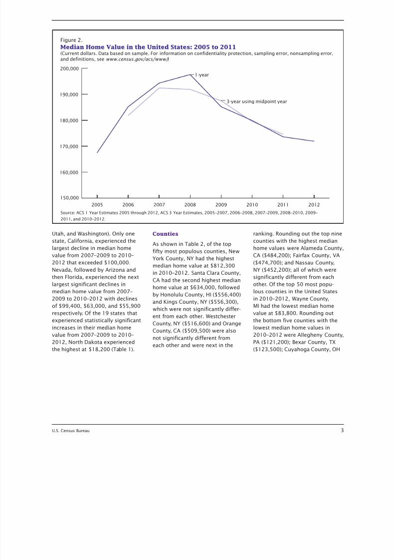
As Figure 1 shows, the median home value in current
dollars, based on decennial census data, rose slowly
from 1940 to 1970. After that, the median home value
rose steadily. By 2000, it had increased by more than
seven times the median home value in 1970. How-
ever, the housing bubble was followed by a housing
crash and the recession. Figure 2, based on ACS data,
which replaced the decennial long form, shows that
after the peak of the reported monetary value in 2008,
the median home value in current dollars declined.
Issued November 2013ACSBR/12-20
By Christine Flanagan and Ellen Wilson
Home Value: Home value is the owner’s estimate
of how much the property (house and lot, mobile
home and lot, or condominium unit) would sell for if
it were for sale. Median home value means that one-
half of all homes were worth more and one-half were
worth less. Median home value estimates in this
report are presented in current dollars.
Homeownership Rate: The homeownership rate
is the percent of occupied housing units that are
owned with a mortgage and those owned free and
clear.
Current dollars: Current dollars are the dollar
values in other time periods that are not converted
into present-day dollars. They do not take into con-
sideration the effects of inflation, but simply present
values as they were at the time. In this report, both
the average over the 3-year period as well as the
comparison across periods are presented in
current dollars.

8/14/2019 Home Value and Homeownership Rates: Recession and Post-Recession Comparisons
http://slidepdf.com/reader/full/home-value-and-homeownership-rates-recession-and-post-recession-comparisons 2/16
2 U.S. Census Bureau
By 2009, the median home value
according to the 2009 American
Community Survey was $185,200.
This was the same estimate that
the 2006 American CommunitySurvey reported as the median
home value in 2006. The median
home value continued to decline
from 2009 to 2012.
States
The median home value for the
United States in 2010–2012 was
$174,600, a $17,300 decline from
the median home value in 2007–
2009. Table 1 shows that in
2010–2012, Hawaii had the highestmedian home value at $503,100,
followed by the District of
Columbia at $436,000. California
came in third place with a median
home value of $358,800, followed
by Massachusetts ($328,300), New Jersey ($325,800), and Maryland
($289,300). Rounding out the top
ten states with the highest median
home values in 2010–2012 were
New York ($286,700), Connecticut
($278,600), Washington
($256,500), and Rhode Island
($245,300). West Virginia had the
lowest median home value at
$98,300, followed by Mississippi at
$100,000, Arkansas at $106,900,
Oklahoma at $112,900, Michigan at
$119,200, and Kentucky at
$120,800. All of these states were
statistically different from each
other.
The median home value decreased
nationally as well as in 28 states
between 2007–2009 and 2010–
2012: 7 in the Northeast
(Connecticut, Maine,
Massachusetts, New Hampshire,
New Jersey, New York, and Rhode
Island), 6 in the South (Delaware,
District of Columbia, Florida,
Georgia, Maryland, and Virginia),
6 in the Midwest (Illinois, Michigan,
Minnesota, Missouri, Ohio, and
Wisconsin), and 9 in the West
(Arizona, California, Colorado,Hawaii, Idaho, Nevada, Oregon,
Figure 1.
Median Home Value in the United States: 1940 to 2010
(Current dollars. Data based on sample. For information on confidentiality protection, sampling error, nonsampling error,
and definitions, see www.census.gov/acs/www/ )
Source: U.S. Census Bureau, Census of Population and Housing, decennial volumes.
0
50,000
100,000
150,000
200,000
20102000199019801970196019501940
2,9387,354
11,90017,000
47,200
79,100
119,600
179,900
8/14/2019 Home Value and Homeownership Rates: Recession and Post-Recession Comparisons
http://slidepdf.com/reader/full/home-value-and-homeownership-rates-recession-and-post-recession-comparisons 3/16
U.S. Census Bureau 3
Utah, and Washington). Only one
state, California, experienced the
largest decline in median home
value from 2007–2009 to 2010–
2012 that exceeded $100,000.Nevada, followed by Arizona and
then Florida, experienced the next
largest significant declines in
median home value from 2007–
2009 to 2010–2012 with declines
of $99,400, $63,000, and $55,900
respectively. Of the 19 states that
experienced statistically significant
increases in their median home
value from 2007–2009 to 2010–
2012, North Dakota experienced
the highest at $18,200 (Table 1).
Counties
As shown in Table 2, of the top
fifty most populous counties, New
York County, NY had the highest
median home value at $812,300in 2010–2012. Santa Clara County,
CA had the second highest median
home value at $634,000, followed
by Honolulu County, HI ($556,400)
and Kings County, NY ($556,300),
which were not significantly differ-
ent from each other. Westchester
County, NY ($516,600) and Orange
County, CA ($509,500) were also
not significantly different from
each other and were next in the
ranking. Rounding out the top nine
counties with the highest median
home values were Alameda County,
CA ($484,200); Fairfax County, VA
($474,700); and Nassau County,NY ($452,200); all of which were
significantly different from each
other. Of the top 50 most popu-
lous counties in the United States
in 2010–2012, Wayne County,
MI had the lowest median home
value at $83,800. Rounding out
the bottom five counties with the
lowest median home values in
2010–2012 were Allegheny County,
PA ($121,200); Bexar County, TX
($123,500); Cuyahoga County, OH
Figure 2.
Median Home Value in the United States: 2005 to 2011
(Current dollars. Data based on sample. For information on confidentiality protection, sampling error, nonsampling error, and definitions, see www.census.gov/acs/www/ )
Source: ACS 1 Year Estimates 2005 through 2012, ACS 3 Year Estimates, 2005–2007, 2006–2008, 2007–2009, 2008–2010, 2009–
2011, and 2010–2012.
150,000
160,000
170,000
180,000
190,000
200,000
3-year using midpoint year
1-year
20122011201020092008200720062005

8/14/2019 Home Value and Homeownership Rates: Recession and Post-Recession Comparisons
http://slidepdf.com/reader/full/home-value-and-homeownership-rates-recession-and-post-recession-comparisons 4/16
4 U.S. Census Bureau
Table 1.
Homeownership Rate and Median Property Value by State: 2007–2009 and 2010–2012
Area
Homeownership rate Median property value (in current dollars)
2007–2009 2010–2012
Difference
2007–2009 2010–2012
DifferenceEstimateMargin oferror (±)1 Estimate
Margin oferror (±)1 Estimate
Margin oferror (±)1 Estimate
Margin oferror (±)1
United States . . . 66.41 0.1 64.68 0.1 *–1.72 191,900 205 174,600 142 *–17,300
Alabama . . . . . . . . . . . . 70.33 0.3 69.57 0.3 *–0.76 118,700 855 123,400 746 *4,700Alaska . . . . . . . . . . . . . . 64.01 0.7 63.50 0.7 –0.51 232,600 1,996 241,400 2,360 *8,800Arizona . . . . . . . . . . . . . 67.55 0.3 63.89 0.3 *–3.66 221,100 952 158,100 710 *–63,000Arkansas . . . . . . . . . . . . 67.14 0.3 66.95 0.4 –0.19 102,900 1,027 106,900 908 *4,000California . . . . . . . . . . . . 57.09 0.1 54.91 0.1 *–2.18 461,400 1,007 358,800 879 *–102,600Colorado . . . . . . . . . . . . 67.66 0.4 64.91 0.3 *–2.75 237,800 713 235,000 1,080 *–2,800Connecticut . . . . . . . . . . 69.16 0.3 67.63 0.3 *–1.53 301,000 1,859 278,600 1,228 *–22,400Delaware . . . . . . . . . . . . 73.07 0.6 71.73 0.6 *–1.35 246,000 2,306 235,900 1,678 *–10,100District of Columbia . . . . 44.86 0.7 41.61 0.7 *–3.25 457,100 6,945 436,000 8,360 *–21,100Florida . . . . . . . . . . . . . . 69.27 0.2 66.89 0.2 *–2.37 210,800 626 154,900 453 *–55,900
Georgia . . . . . . . . . . . . . 67.35 0.3 64.94 0.2 *–2.41 165,100 560 149,300 792 *–15,800Hawaii . . . . . . . . . . . . . . 57.87 0.6 57.28 0.6 –0.59 543,600 5,606 503,100 5,879 *–40,500Idaho . . . . . . . . . . . . . . . 71.13 0.5 68.97 0.5 *–2.16 177,400 1,391 160,000 941 *–17,400Illinois. . . . . . . . . . . . . . . 68.84 0.2 67.33 0.2 *–1.51 207,300 617 179,900 715 *–27,400Indiana . . . . . . . . . . . . . . 71.10 0.3 69.91 0.3 *–1.19 122,800 471 122,600 478 –200Iowa . . . . . . . . . . . . . . . . 72.78 0.3 72.30 0.3 *–0.48 120,100 572 124,300 688 *4,200
Kansas. . . . . . . . . . . . . . 68.94 0.4 67.42 0.4 *–1.52 123,600 862 128,500 997 *4,900Kentucky . . . . . . . . . . . . 69.50 0.3 68.12 0.3 *–1.38 116,800 641 120,800 548 *4,000Louisiana . . . . . . . . . . . . 67.98 0.3 66.72 0.3 *–1.26 131,800 1,143 138,800 1,140 *7,000Maine . . . . . . . . . . . . . . . 72.77 0.4 71.57 0.5 *–1.19 178,100 1,776 173,900 1,199 *–4,200
Maryland . . . . . . . . . . . . 69.19 0.3 67.07 0.3 *–2.11 335,100 1,175 289,300 1,168 *–45,800Massachusetts. . . . . . . . 64.68 0.2 62.32 0.2 *–2.36 352,400 932 328,300 1,184 *–24,100Michigan . . . . . . . . . . . . 73.94 0.2 71.88 0.2 *–2.06 145,400 379 119,200 401 *–26,200Minnesota . . . . . . . . . . . 74.18 0.2 72.39 0.2 *–1.79 209,900 557 185,800 692 *–24,100Mississippi . . . . . . . . . . . 70.13 0.4 69.23 0.4 *–0.91 97,300 888 100,000 1,091 *2,700Missouri . . . . . . . . . . . . . 69.74 0.2 68.38 0.2 *–1.36 139,700 626 137,100 656 *–2,600Montana. . . . . . . . . . . . . 68.55 0.6 68.18 0.6 –0.37 174,900 1,682 183,600 2,139 *8,700Nebraska . . . . . . . . . . . . 67.91 0.4 66.76 0.4 *–1.14 122,600 702 127,800 765 *5,200Nevada . . . . . . . . . . . . . 59.59 0.4 56.17 0.4 *–3.42 260,700 1,962 161,300 998 *–99,400New Hampshire . . . . . . . 72.83 0.6 71.36 0.5 *–1.47 257,600 1,878 239,100 1,338 *–18,500
New Jersey . . . . . . . . . . 66.75 0.2 65.56 0.2 *–1.19 361,100 921 325,800 908 *–35,300
New Mexico . . . . . . . . . . 69.16 0.5 68.07 0.4 *–1.09 160,900 1,384 159,300 1,201 –1,600New York . . . . . . . . . . . . 55.39 0.1 53.90 0.1 *–1.50 310,100 1,639 286,700 1,398 *–23,400North Carolina . . . . . . . . 67.70 0.2 66.33 0.2 *–1.37 151,800 603 152,800 638 *1,000North Dakota . . . . . . . . . 65.95 0.6 65.69 0.6 –0.26 112,300 1,509 130,500 1,816 *18,200Ohio . . . . . . . . . . . . . . . . 68.85 0.2 67.30 0.2 *–1.55 136,900 362 130,600 470 *–6,300Oklahoma . . . . . . . . . . . 67.45 0.3 67.07 0.3 –0.37 104,900 681 112,900 541 *8,000Oregon. . . . . . . . . . . . . . 63.90 0.3 61.65 0.4 *–2.26 263,200 1,317 233,900 1,296 *–29,300Pennsylvania . . . . . . . . . 70.94 0.2 69.55 0.2 *–1.39 161,700 551 164,700 368 *3,000Rhode Island . . . . . . . . . 63.04 0.7 60.32 0.6 *–2.72 282,300 1,875 245,300 1,637 *–37,000
South Carolina . . . . . . . . 70.07 0.3 68.78 0.3 *–1.29 136,300 797 136,300 951 0South Dakota . . . . . . . . . 68.21 0.5 68.02 0.5 –0.18 122,500 1,425 131,600 1,445 *9,100Tennessee . . . . . . . . . . . 69.50 0.3 67.48 0.3 *–2.02 135,400 671 138,400 678 *3,000Texas . . . . . . . . . . . . . . . 64.22 0.1 63.01 0.2 *–1.21 124,400 355 128,400 482 *4,000Utah . . . . . . . . . . . . . . . . 71.77 0.4 69.69 0.4 *–2.09 227,400 1,025 209,000 1,134 *–18,400Vermont . . . . . . . . . . . . . 71.68 0.7 70.92 0.7 –0.77 211,800 1,964 215,700 2,038 *3,900Virginia. . . . . . . . . . . . . . 68.55 0.2 67.11 0.2 *–1.44 260,100 1,205 243,100 1,042 *–17,000
Washington . . . . . . . . . . 65.06 0.3 62.80 0.3 *–2.25 297,000 1,131 256,500 1,152 *–40,500West Virginia . . . . . . . . . 73.91 0.4 72.93 0.5 *–0.97 95,400 940 98,300 958 *2,900Wisconsin . . . . . . . . . . . 69.40 0.2 67.96 0.2 *–1.44 170,800 471 167,200 475 *–3,600Wyoming . . . . . . . . . . . . 69.80 0.8 69.98 0.7 0.17 181,900 2,636 183,200 2,453 1,300
* Statistically different from zero at the 90 percent confidence level.1 Data are based on a sample and are subject to sampling variability. A margin of error is a measure of an estimate’s variability. The larger the margin of error
in relation to the size of the estimate, the less reliable the estimate. When added to and subtracted from the estimate, the margin of error forms the 90 percent
confidence interval.Sources: U.S. Census Bureau, 2007–2009 and 2010–2012 American Community Surveys.

8/14/2019 Home Value and Homeownership Rates: Recession and Post-Recession Comparisons
http://slidepdf.com/reader/full/home-value-and-homeownership-rates-recession-and-post-recession-comparisons 5/16
U.S. Census Bureau 5
Table 2.
Homeownership Rate and Median Property Value by 50 Most Populous Counties: 2007–
2009 and 2010–20121
Area
Homeownership rate Median property value (in current dollars)
2007–2009 2010–2012
Differ-ence
2007–2009 2010–2012
DifferenceEstimateMargin oferror (±)2 Estimate
Margin oferror (±)2 Estimate
Margin oferror (±)2 Estimate
Margin oferror (±)2
United States . . . . . . . . . . . . . . 66.41 0.1 64.68 0.1 *–1.72 191,900 205 174,600 142 *–17,300
Los Angeles County, California . . . . . . 47.82 0.2 46.42 0.2 *–1.40 517,900 2,884 414,100 1,679 *–103,800Cook County, Illinois . . . . . . . . . . . . . . 60.23 0.3 57.88 0.3 *–2.35 274,400 1,327 227,400 1,201 *–47,000Harris County, Texas . . . . . . . . . . . . . . 57.09 0.3 56.30 0.4 *–0.79 133,700 820 131,000 942 *–2,700Maricopa County, Arizona . . . . . . . . . . 66.47 0.3 61.74 0.4 *–4.73 243,400 1,228 167,100 955 *–76,300San Diego County, California. . . . . . . . 55.95 0.3 53.58 0.4 *–2.37 484,700 2,680 396,500 2,043 *–88,200Orange County, California . . . . . . . . . . 60.87 0.4 58.33 0.4 *–2.55 608,800 2,583 509,500 3,575 *–99,300Miami-Dade County, Florida . . . . . . . . 57.87 0.5 55.71 0.6 *–2.16 279,800 1,921 188,400 2,264 *–91,400Kings County, New York . . . . . . . . . . . . 30.37 0.4 29.49 0.3 *–0.88 580,900 4,034 556,300 4,291 *–24,600Dallas County, Texas . . . . . . . . . . . . . . 54.09 0.4 52.52 0.4 *–1.57 130,600 1,249 128,000 1,583 *–2,600Queens County, New York . . . . . . . . . . 45.67 0.5 43.33 0.4 *–2.34 491,100 4,546 447,500 3,089 *–43,600
Riverside County, California . . . . . . . . 69.19 0.5 66.26 0.6 *–2.94 330,100 2,674 223,700 1,873 *–106,400San Bernardino County, California . . . 64.34 0.6 61.77 0.6 *–2.56 323,800 2,813 211,700 2,879 *–112,100Clark County, Nevada . . . . . . . . . . . . . 57.62 0.5 53.79 0.6 *–3.83 262,800 2,235 156,500 1,252 *–106,300King County, Washington . . . . . . . . . . . 60.62 0.4 57.41 0.5 *–3.22 423,600 2,408 369,000 2,547 *–54,600Tarrant County, Texas . . . . . . . . . . . . . 62.77 0.4 61.36 0.5 *–1.41 135,700 806 135,100 1,107 –600
Santa Clara County, California . . . . . . 59.39 0.6 56.87 0.5 *–2.51 707,900 4,271 634,000 4,342 *–73,900Wayne County, Michigan . . . . . . . . . . . 66.86 0.5 64.34 0.4 *–2.52 118,100 972 83,800 727 *–34,300Broward County, Florida . . . . . . . . . . . 69.55 0.5 65.44 0.5 *–4.11 252,800 3,246 170,800 1,521 *–82,000Bexar County, Texas . . . . . . . . . . . . . . 61.64 0.5 59.18 0.6 *–2.47 117,500 1,110 123,500 1,490 *6,000New York County, New York . . . . . . . . . 23.92 0.4 22.03 0.4 *–1.89 840,100 15,423 812,300 17,978 *–27,800
Philadelphia County, Pennsylvania . . . 55.59 0.5 53.42 0.5 *–2.17 143,300 2,265 142,300 2,205 –1,000Alameda County, California . . . . . . . . . 55.08 0.6 52.81 0.5 *–2.27 594,600 4,166 484,200 4,995 *–110,400Middlesex County, Massachusetts . . . 64.29 0.5 62.52 0.5 *–1.77 419,400 2,814 396,400 2,451 *–23,000Suffolk County, New York . . . . . . . . . . . 82.18 0.4 78.89 0.5 *–3.29 430,600 2,555 383,000 1,718 *–47,600Sacramento County, California . . . . . . 59.14 0.6 56.30 0.6 *–2.83 321,100 2,789 224,800 2,298 *–96,300Bronx County, New York . . . . . . . . . . . 21.30 0.4 19.02 0.5 *–2.28 397,300 7,958 373,500 5,185 *–23,800Nassau County, New York . . . . . . . . . . 83.17 0.5 80.37 0.4 *–2.80 494,000 2,310 452,200 2,020 *–41,800Palm Beach County, Florida . . . . . . . . 72.73 0.5 71.01 0.5 *–1.72 263,800 2,556 190,500 2,753 *–73,300Cuyahoga County, Ohio . . . . . . . . . . . . 61.21 0.5 60.66 0.4 –0.55 136,600 946 125,700 1,080 *–10,900Hillsborough County, Florida . . . . . . . . 62.40 0.6 59.84 0.6 *–2.57 204,200 2,230 154,900 1,500 *–49,300
Allegheny County, Pennsylvania . . . . . 66.33 0.5 65.24 0.4 *–1.09 116,300 1,092 121,200 1,111 *4,900Oakland County, Michigan . . . . . . . . . . 74.64 0.5 71.11 0.5 *–3.52 207,100 1,973 165,300 1,021 *–41,800Franklin County, Ohio . . . . . . . . . . . . . 57.55 0.6 54.29 0.5 *–3.26 157,000 1,143 151,200 1,459 *–5,800Orange County, Florida . . . . . . . . . . . . 60.09 0.7 57.32 0.7 *–2.77 237,200 2,418 161,000 1,463 *–76,200Hennepin County, Minnesota. . . . . . . . 65.73 0.5 63.49 0.5 *–2.25 250,900 2,224 228,100 1,570 *–22,800Fairfax County, Virginia . . . . . . . . . . . . 71.54 0.7 68.29 0.7 *–3.25 510,600 5,122 474,700 3,668 *–35,900Contra Costa County, California . . . . . 69.45 0.7 65.08 0.7 *–4.38 534,400 6,986 392,900 5,138 *–141,500Travis County, Texas . . . . . . . . . . . . . . 52.89 0.6 51.17 0.8 *–1.72 206,600 3,169 215,700 3,602 *9,100Salt Lake County, Utah . . . . . . . . . . . . 68.46 0.7 66.68 0.7 *–1.78 247,500 1,753 228,300 1,734 *–19,200St. Louis County, Missouri . . . . . . . . . . 72.34 0.6 70.84 0.6 *–1.50 181,600 1,845 174,100 1,475 *–7,500
Montgomery County, Maryland . . . . . . 70.11 0.6 66.55 0.6 *–3.56 484,700 4,101 444,100 4,298 *–40,600Pima County, Arizona . . . . . . . . . . . . . 65.36 0.6 62.11 0.7 *–3.25 204,000 2,023 164,800 1,712 *–39,200Honolulu County, Hawaii . . . . . . . . . . . 55.79 0.7 55.29 0.6 –0.49 565,600 5,881 556,400 5,246 *–9,200Westchester County, New York . . . . . . 62.47 0.6 62.06 0.6 –0.41 562,700 6,781 516,600 6,280 *–46,100Milwaukee County, Wisconsin . . . . . . . 53.56 0.6 50.97 0.6 *–2.59 168,100 1,040 158,700 1,188 *–9,400Fulton County, Georgia . . . . . . . . . . . . 57.56 0.8 53.23 0.7 *–4.33 260,400 5,464 235,600 4,822 *–24,800
Mecklenburg County, North Carolina . . 62.30 0.6 59.89 0.7 *–2.41 190,000 2,237 181,600 2,931 *–8,400Fresno County, California . . . . . . . . . . 54.54 0.8 53.58 0.8 –0.96 261,300 3,908 190,400 3,186 *–70,900Shelby County, Tennessee . . . . . . . . . 60.99 0.7 58.62 0.7 *–2.37 134,700 2,034 132,500 1,935 –2,200Wake County, North Carolina . . . . . . . 66.53 0.7 65.29 0.8 *–1.24 226,200 2,443 228,800 2,431 2,600
* Statistically different from zero at the 90 percent confidence level.1 Ranked in order of population—highest to lowest.2 Data are based on a sample and are subject to sampling variability. A margin of error is a measure of an estimate’s variability. The larger the margin of error in
relation to the size of the estimate, the less reliable the estimate. When added to and subtracted from the estimate, the margin of error forms the 90 percent confi-
dence interval.
Sources: U.S. Census Bureau, 2007–2009 and 2010–2012 American Community Surveys.

8/14/2019 Home Value and Homeownership Rates: Recession and Post-Recession Comparisons
http://slidepdf.com/reader/full/home-value-and-homeownership-rates-recession-and-post-recession-comparisons 6/16
6 U.S. Census Bureau
Table 3.
Homeownership Rate and Median Property Value by 50 Least Populous Counties: 2007–
2009 and 2010–20121
Area
Homeownership rate Median property value (in current dollars)
2007–2009 2010–2012
Differ-ence
2007–2009 2010–2012
Differ-enceEstimate
Margin oferror (±)2 Estimate
Margin oferror (±)2 Estimate
Margin oferror (±)2 Estimate
Margin oferror (±)2
United States . . . . . . . . . . . . 66.41 0.1 64.68 0.1 *–1.72 191,900 205 174,600 142 *–17,300
Covington County, Mississippi . . . . . 83.44 4.8 83.07 3.9 –0.36 79,400 6,216 74,100 6,779 –5,300Plumas County, California . . . . . . . . 67.66 5.8 71.70 4.6 4.03 279,500 25,394 237,100 18,649 *–42,400Jackson County, Iowa . . . . . . . . . . . 78.68 3.1 73.82 3.0 *–4.86 111,500 6,856 104,800 7,482 –6,700Langlade County, Wisconsin . . . . . . 79.44 3.0 74.83 2.9 *–4.61 116,300 6,199 112,800 7,034 –3,500Elbert County, Georgia . . . . . . . . . . 75.15 3.7 66.47 3.9 *–8.68 87,300 12,309 83,000 3,960 –4,300Gonzales County, Texas . . . . . . . . . 63.81 6.0 72.28 4.3 *8.47 77,600 9,082 82,000 7,433 4,400Lampasas County, Texas . . . . . . . . . 74.92 4.6 74.98 3.9 0.07 118,400 13,369 125,900 12,071 7,500Marion County, Kentucky . . . . . . . . . 79.12 4.3 76.05 3.9 –3.07 93,000 8,458 100,900 6,610 7,900Minidoka County, Idaho . . . . . . . . . . 78.31 3.8 71.13 4.5 *–7.18 99,500 8,397 107,900 6,533 8,400Carroll County, Indiana . . . . . . . . . . 77.21 3.7 79.65 3.2 2.44 109,000 6,819 105,900 6,306 –3,100
Breckinridge County, Kentucky . . . . 77.85 4.2 82.41 2.8 4.56 81,800 6,689 81,600 5,359 –200East Feliciana Parish, Louisiana . . . 84.15 3.7 77.95 3.2 *–6.2 98,400 9,605 123,800 20,599 * 25,400Allen County, Kentucky . . . . . . . . . . 75.08 4.4 73.93 3.8 –1.15 90,800 4,960 91,800 5,164 1,000Jones County, Texas . . . . . . . . . . . . 82.41 3.6 76.53 4.4 *–5.88 55,700 8,297 65,500 8,171 9,800Dodge County, Minnesota . . . . . . . . 86.78 2.4 84.64 2.4 –2.14 166,100 5,715 159,700 5,517 –6,400
Woodward County, Oklahoma . . . . . 69.55 4.5 72.59 4.3 3.04 97,000 7,196 105,000 10,023 8,000Kent County, Maryland . . . . . . . . . . 72.63 4.2 70.55 4.0 –2.08 286,600 25,109 254,000 17,326 *–32,600Henry County, Iowa . . . . . . . . . . . . . 71.10 3.6 75.24 3.4 4.15 99,100 5,422 100,000 5,452 900Washington County, Nebraska . . . . 80.58 3.2 81.69 2.6 1.11 168,600 8,741 174,000 9,665 5,400DeWitt County, Texas . . . . . . . . . . . . 76.44 4.4 73.85 5.0 –2.6 71,000 6,936 79,200 8,591 8,200
Roosevelt County, New Mexico . . . . 63.06 4.4 57.16 5.2 –5.89 87,800 8,060 117,500 8,423 *29,700Polk County, North Carolina . . . . . . 77.04 5.2 75.20 4.4 –1.84 180,500 25,644 167,000 19,404 –13,500Morgan County, Missouri . . . . . . . . . 83.11 2.8 82.73 2.8 –0.38 116,200 12,182 114,000 10,058 –2,200Hubbard County, Minnesota . . . . . . 83.96 2.4 82.53 2.0 –1.43 171,300 6,618 175,000 7,091 3,700Buena Vista County, Iowa . . . . . . . . 67.67 3.9 71.35 3.6 3.68 85,800 3,938 97,600 5,084 *11,800McIntosh County, Oklahoma . . . . . . 76.54 3.4 79.29 3.4 2.75 70,200 8,184 82,400 7,251 *12,200Lincoln County, New Mexico . . . . . . 77.81 3.8 78.92 3.6 1.12 162,200 21,004 157,600 11,495 –4,600La Paz County, Arizona . . . . . . . . . . 72.17 4.7 75.21 4.2 3.05 97,100 19,165 95,600 13,414 –1,500Jackson County, Wisconsin . . . . . . . 76.23 2.9 74.08 2.5 –2.15 123,500 4,855 125,000 6,792 1500Clay County, Mississippi . . . . . . . . . 70.62 4.9 70.93 3.9 0.31 76,100 8,062 80,700 4,959 4,600
Bandera County, Texas . . . . . . . . . . 83.56 3.9 76.98 4.0 *–6.58 142,000 19,031 142,600 23,057 600Polk County, Arkansas . . . . . . . . . . . 77.29 4.1 75.94 4.0 –1.35 82,700 6,556 85,300 5,919 2,600Kewaunee County, Wisconsin . . . . . 81.05 2.7 81.45 2.9 0.4 143,500 8,524 146,600 7,000 3,100Klickitat County, Washington . . . . . . 69.64 4.2 67.33 4.4 –2.31 188,100 13,231 197,900 14,725 9,800Butler County, Alabama . . . . . . . . . . 68.04 4.3 70.47 4.2 2.43 77,500 9,585 73,900 4,677 –3,600Taylor County, Wisconsin . . . . . . . . . 80.28 2.4 77.71 2.2 –2.57 121,800 3,643 127,500 5,442 5,700Clinton County, Missouri . . . . . . . . . 74.84 3.3 72.19 3.6 –2.65 153,000 8,839 143,300 9,387 –9,700Martin County, Minnesota . . . . . . . . 76.21 3.3 75.70 2.5 –0.51 96,600 4,946 105,800 5,875 *9,200Concordia Parish, Louisiana . . . . . . 65.61 5.0 63.30 4.9 –2.31 79,400 9,151 78,800 8,530 –600Jones County, Iowa . . . . . . . . . . . . . 80.51 3.3 80.33 2.8 –0.18 104,200 8,609 124,600 11,517 *20,400
Marengo County, Alabama . . . . . . . 69.98 5.1 70.10 3.6 0.13 79,300 7,936 95,900 11,215 *16,600Wayne County, Mississippi . . . . . . . 81.40 5.2 83.45 3.8 2.05 57,800 7,015 68,700 7,026 * 10,900Franklin Parish, Louisiana . . . . . . . . 71.94 4.2 73.02 3.8 1.09 73,600 5,301 77,900 7,836 4,300Carroll County, Iowa . . . . . . . . . . . . 72.37 3.1 77.60 3.1 *5.24 108,800 5,165 105,400 6,717 –3,400Crook County, Oregon . . . . . . . . . . . 75.18 3.9 69.60 3.8 *–5.59 237,600 13,443 172,700 18,334 *–64,900Colorado County, Texas . . . . . . . . . . 77.94 3.8 76.15 4.5 –1.79 84,900 10,731 112,600 15,490 *27,700
Madison County, North Carolina . . . 78.71 4.0 72.21 4.6 *–6.5 173,600 17,812 155,100 11,789 –18,500Fulton County, Indiana . . . . . . . . . . . 80.03 3.7 73.44 4.3 *–6.6 97,900 5,850 93,300 7,853 –4,600Pacific County, Washington . . . . . . . 75.53 2.9 72.73 3.4 –2.8 170,100 7,117 158,100 7,493 *–12,000Warren County, North Carolina . . . . 77.30 4.2 67.82 4.3 *–9.49 93,300 9,947 106,800 9,548 13,500
* Statistically different from zero at the 90 percent confidence level.1 Ranked in order of population—lowest to highest.2 Data are based on a sample and are subject to sampling variability. A margin of error is a measure of an estimate’s variability. The larger the margin of error
in relation to the size of the estimate, the less reliable the estimate. When added to and subtracted from the estimate, the margin of error forms the 90 percent
confidence interval.
Sources: U.S. Census Bureau, 2007–2009 and 2010–2012 American Community Surveys.

8/14/2019 Home Value and Homeownership Rates: Recession and Post-Recession Comparisons
http://slidepdf.com/reader/full/home-value-and-homeownership-rates-recession-and-post-recession-comparisons 7/16
U.S. Census Bureau 7
($125,700); and Dallas County, TX
($128,000); all of which were sig-
nificantly different from each other.
Worth noting is that out of the top
50 most populous counties, 43
counties experienced significant
declines in their overall median
home value from 2007–2009 to2010–2012. The largest decline
was in Contra Costa County, CA,
which declined by $141,500.
Only Bexar County, TX; Alleghany
County, PA; and Travis County, TX;
experienced significant increases
in their median home value
from 2007–2009 to 2010–2012
(Table 2).
Of the 1,038 smaller counties in
2010–2012, which include the 50
least populous counties shownin Table 3, 344 (33.1 percent)
experienced significant changes
in their median home value from
2007–2009 to 2010–2012. A little
over half (183 counties or 53.2 per-
cent) of these counties experienced
significant declines in their median
home value, while 46.8 percent
(161 counties) experienced sig-
nificant increases in their median
home value.
McDowell County, WV had the low-
est median home value at $39,900
of these smaller counties. Five of
these counties had median home
values that were over $400,000.
The highest was Teton County, WY
at $705,600. Teton County was
followed by Summit County, UT
at $488,700, Eagle County, CO
at $469,800, Fairfax City, VA3 at
$450,900, and Summit County,
CO at $ 442,800, none of which
3 Fairfax city, VA is a county equivalentand is included in the discussion of counties.
were significantly different from
one another.
Table 3 shows that of the fifty least
populous counties in 2010–2012,
Kent County, MD and Plumas
County, CA had the highest median
home values at $254,000 and
$237,100 respectively and werenot significantly different from each
other. Rounding out the bottom
three counties with the highest
median value was Klickitat County,
WA with a median home value of
$197,900.
Only 4 of the 50 least populous
counties experienced significant
declines in median home value
from 2007–2009 to 2010–2012.
They were Crook County, OR
(–$64,900); Plumas County, CA(–$42,400); Kent County, MD
(–$32,600); and Pacific County,
WA (–$12,000). Conversely, nine
counties experienced significant
increases in median home value
from 2007–2009 to 2010–2012.
Metropolitan Areas
Of the top 50 most populous
metro areas in 2010–2012, Table 4
shows that the San Jose-Sunnyvale-
Santa Clara, CA Metro Area had
the highest median home value
at $624,800. The San Francisco-
Oakland-Fremont, CA Metro Area
had the second highest median
home value at $568,900. These
were followed by the Los Angeles-
Long Beach-Santa Ana, CA Metro
Area ($442,000) with the third
highest median home value and the
New York-Northern New Jersey-
Long Island, NY-NJ-PA Metro Area
($412,500) with the fourth highestmedian home value. Rounding out
the top nine metro areas with the
highest median home values were
the San Diego-Carlsbad-San
Marcos, CA Metro Area ($396,500),
the Washington-Arlington-
Alexandria, DC-VA-MD-WV Metro
Area ($369,500), the Boston-
Cambridge-Quincy, MA-NH Metro
Area ($360,100), the Seattle-
Tacoma-Bellevue, WA Metro Area
($312,700), and the Baltimore-
Towson, MD Metro Area
($279,300), all significantly dif-
ferent from each other. The 3 of
the top 50 most populous metro
areas with the lowest median home
values in 2010–2012 were the
Detroit-Warren-Livonia, MI Metro
Area ($119,900), followed by the
Buffalo-Niagara Falls, NY Metro
Area ($121,500), and then the
Pittsburgh, PA Metro Area($124,300) with the third lowest
median home value, all significantly
different from each other.
Of the top 50 most populous metro
areas, 36 metro areas experienced
significant declines in median
home value from 2007–2009 to
2010–2012. Three of these sig-
nificant declines amounted to
over $100,000. These metro areas
were the Riverside-San Bernardino-
Ontario, CA Metro Area, the Las
Vegas-Paradise, NV Metro Area,
and the Los Angeles-Long Beach-
Santa Ana, CA Metro Area. Only the
Riverside-San Bernardino-Ontario,
CA Metro Area and the Los Angeles-
Long Beach-Santa Ana, CA Metro
Areas were statistically different
from each other. Conversely, ten
metro areas experienced significant
increases in median home value.
Places (Cities)
Table 5 shows that the 3 cities of
the top 50 most populous cities

8/14/2019 Home Value and Homeownership Rates: Recession and Post-Recession Comparisons
http://slidepdf.com/reader/full/home-value-and-homeownership-rates-recession-and-post-recession-comparisons 8/16
8 U.S. Census Bureau
Table 4.
Homeownership Rate and Median Property Value by 50 Most Populous Metropolitan
Statistical Area: 2007–2009 and 2010–20121—Con.
Area
Homeownership rate Median property value (in current dollars)
2007–2009 2010–2012
Differ-ence
2007–2009 2010–2012
DifferenceEstimate
Marginof error
(±)2 Estimate
Marginof error
(±)2 Estimate
Marginof error
(±)2 Estimate
Marginof error
(±)2
United States . . . . . . . . . . . . . . . . . . . 66.41 0.1 64.68 0.1 *–1.72 191,900 205 174,600 142 *–17,300
New York-Northern New Jersey-Long Island,NY-NJ-PA Metro Area . . . . . . . . . . . . . . . . . 53.08 0.1 51.59 0.1 *–1.49 455,900 1,060 412,500 1,011 *–43,400
Los Angeles-Long Beach-Santa Ana, CAMetro Area. . . . . . . . . . . . . . . . . . . . . . . . . . 50.89 0.2 49.23 0.2 *–1.66 546,500 2,065 442,000 1,294 *–104,500
Chicago-Joliet-Naperville, IL-IN-WI MetroArea . . . . . . . . . . . . . . . . . . . . . . . . . . . . . . . 67.69 0.2 65.69 0.2 *–2.00 258,800 957 221,800 956 *–37,000
Dallas-Fort Worth-Arlington, TXMetro Area. . . . . . . . . . . . . . . . . . . . . . . . . . 62.46 0.2 60.93 0.2 *–1.54 148,100 634 149,200 722 *1,100
Houston-Sugar Land-Baytown, TX MetroArea . . . . . . . . . . . . . . . . . . . . . . . . . . . . . . . 62.50 0.3 61.91 0.3 *–0.59 139,400 728 140,700 842 *1,300
Philadelphia-Camden-Wilmington, PA-NJ-DE-MD Metro Area . . . . . . . . . . . . . . . . . . . 69.77 0.3 68.10 0.2 *–1.67 247,700 900 239,700 883 *–8,000
Washington-Arlington-Alexandria, DC-VA-MD-WV Metro Area . . . . . . . . . . . . . . . . . . . 66.57 0.3 63.67 0.3 *–2.90 421,600 1,694 369,500 1,421 *–52,100
Miami-Fort Lauderdale-Pompano Beach, FL
Metro Area. . . . . . . . . . . . . . . . . . . . . . . . . . 65.52 0.3 62.90 0.3 *–2.62 266,800 1,366 182,500 1,321 *–84,300Atlanta-Sandy Springs-Marietta, GA Metro
Area . . . . . . . . . . . . . . . . . . . . . . . . . . . . . . . 68.46 0.3 65.06 0.3 *–3.40 193,000 818 168,100 904 *–24,900Boston-Cambridge-Quincy, MA-NH Metro
Area . . . . . . . . . . . . . . . . . . . . . . . . . . . . . . . 63.84 0.3 61.51 0.3 *–2.33 382,400 1,066 360,100 1,084 *–22,300
San Francisco-Oakland-Fremont, CAMetro Area. . . . . . . . . . . . . . . . . . . . . . . . . . 56.17 0.4 53.68 0.3 *–2.49 656,300 3,105 568,900 3,547 *–87,400
Riverside-San Bernardino-Ontario, CAMetro Area. . . . . . . . . . . . . . . . . . . . . . . . . . 66.89 0.4 64.15 0.4 *–2.74 327,200 1,772 218,800 1,726 *–108,400
Detroit-Warren-Livonia, MI Metro Area . . . . . 72.98 0.3 70.21 0.3 *–2.77 158,000 622 119,900 680 *–38,100Phoenix-Mesa-Glendale, AZ Metro Area . . . . 67.26 0.4 62.85 0.4 *–4.41 237,100 1,140 161,700 907 *–75,400Seattle-Tacoma-Bellevue, WA Metro Area . . 62.62 0.3 60.05 0.3 *–2.57 371,000 1,361 312,700 1,982 *–58,300Minneapolis-St. Paul-Bloomington, MN-WI
Metro Area. . . . . . . . . . . . . . . . . . . . . . . . . . 72.98 0.3 70.52 0.3 *–2.46 242,300 683 213,900 944 *–28,400San Diego-Carlsbad-San Marcos, CA
Metro Area. . . . . . . . . . . . . . . . . . . . . . . . . . 55.95 0.3 53.58 0.4 *–2.37 484,700 2,680 396,500 2,043 *–88,200
Tampa-St. Petersburg-Clearwater, FLMetro Area. . . . . . . . . . . . . . . . . . . . . . . . . . 68.97 0.4 66.12 0.4 *–2.85 187,200 1,190 141,200 1,242 *–46,000
St. Louis, MO-IL Metro Area . . . . . . . . . . . . . 71.95 0.4 70.34 0.4 *–1.61 160,900 767 157,800 873 *–3,100Baltimore-Towson, MD Metro Area . . . . . . . . 68.09 0.4 66.35 0.4 *–1.74 307,900 1,913 279,300 1,492 *–28,600
Denver-Aurora-Broomfield, CO Metro Area . . 66.72 0.4 63.42 0.4 *–3.30 246,700 883 245,700 1,206 –1,000Pittsburgh, PA Metro Area . . . . . . . . . . . . . . . 70.97 0.4 69.75 0.3 *–1.22 118,100 744 124,300 793 *6,200Portland-Vancouver-Hillsboro, OR-WA
Metro Area. . . . . . . . . . . . . . . . . . . . . . . . . . 63.68 0.4 61.03 0.4 *–2.64 296,900 1,741 260,600 1,722 *–36,300San Antonio-New Braunfels, TX
Metro Area. . . . . . . . . . . . . . . . . . . . . . . . . . 64.82 0.5 62.90 0.5 *–1.92 123,400 1,091 131,800 1,656 *8,400Orlando-Kissimmee-Sanford, FL
Metro Area. . . . . . . . . . . . . . . . . . . . . . . . . . 66.24 0.5 63.09 0.5 *–3.15 225,200 1,587 155,600 1,204 *–69,600Sacramento—Arden-Arcade—Roseville, CA
Metro Area. . . . . . . . . . . . . . . . . . . . . . . . . . 62.46 0.5 59.89 0.4 *–2.57 356,000 2,053 261,700 2,192 *–94,300Cincinnati-Middletown, OH-KY-IN Metro
Area . . . . . . . . . . . . . . . . . . . . . . . . . . . . . . . 68.87 0.5 67.96 0.4 *–0.91 157,500 827 153,100 980 *–4,400
Cleveland-Elyria-Mentor, OH Metro Area . . . 67.25 0.4 66.41 0.4 *–0.85 150,100 1,006 141,700 788 *–8,400Kansas City, MO-KS Metro Area . . . . . . . . . . 68.60 0.4 67.10 0.4 *–1.50 160,000 831 157,600 849 *–2,400Las Vegas-Paradise, NV Metro Area . . . . . . . 57.62 0.5 53.79 0.6 *–3.83 262,800 2,235 156,500 1,252 *–106,300
San Jose-Sunnyvale-Santa Clara, CAMetro Area. . . . . . . . . . . . . . . . . . . . . . . . . . 59.53 0.5 57.06 0.5 *–2.47 702,700 4,247 624,800 4,296 *–77,900
Columbus, OH Metro Area . . . . . . . . . . . . . . 64.28 0.5 61.89 0.4 *–2.39 164,400 950 160,500 965 *–3,900Charlotte-Gastonia-Rock Hill, NC-SC
Metro Area. . . . . . . . . . . . . . . . . . . . . . . . . . 67.31 0.4 65.93 0.5 *–1.38 173,000 1,150 168,300 1,442 *–4,700Austin-Round Rock-San Marcos, TX
Metro Area. . . . . . . . . . . . . . . . . . . . . . . . . . 59.30 0.5 57.40 0.6 *–1.89 184,000 1,847 188,700 1,966 *4,700
See notes at end of table.

8/14/2019 Home Value and Homeownership Rates: Recession and Post-Recession Comparisons
http://slidepdf.com/reader/full/home-value-and-homeownership-rates-recession-and-post-recession-comparisons 9/16
U.S. Census Bureau 9
that had the largest median home
values in 2010–2012 were San
Francisco City, CA ($737,700),
followed by San Jose City, CA
($546,300), and then New York
City, NY ($490,400). The city that
had the lowest median home value
of the 50 most populous cities in
2010–2012 was Detroit City, MI at
$48,000. Cleveland City, OH had
the second lowest median home
value ($76,700), followed by
Memphis City, TN ($96,800), and
San Antonio City, TX ($113,400).
Thirty-five of the top fifty most
populous cities experienced signifi-
cant declines in their median home
value from 2007–2009 to 2010–
2012. Seven cities experienced
significant increases in median
home value. The cities with the
highest increase in median home
values were Austin City, TX with
a $13,800 increase and Denver
City, CO with a $9,600 increase,
which were not significantly differ-
ent from each other. Additionally,
Denver City was not significantly
different from Oklahoma City, OK;
Tulsa City, OK; El Paso City TX; or
Wichita City, KS.
Of the 1,596 smaller cities in 2010–
2012, which include the 50 least
populous cities shown on Table 6,
1,023 (64.1 percent) experienced
significant changes in their medianhome value from 2007–2009 to
2010–2012. Of these cities, 90.9
percent (930 cities) experienced
significant declines in their median
home value. Conversely, 93 cities
(9.1 percent) experienced sig-
nificant increases in their median
home value. Sixty-one cities
were not discussed in this report
because comparable statistics for
previous years were not available.
Table 6 shows that Lake Forest City,
IL had the highest median home
value in 2010–2012 of the 50 least
populous cities at $837,600.4 In
second place was Naples City, FL at
$722,100 followed by Syosset CDP,
NY ($609,700) and La Crescenta-
Montrose CDP, CA ($608,700),
which were not significantly differ-
ent from one another. Rounding out
the top five was Marblehead CDP,
4 Six places that would have beenincluded in the fifty least populous cities werenot included because comparable statisticsfor previous years were not comparable.
Table 4.
Homeownership Rate and Median Property Value by 50 Most Populous Metropolitan
Statistical Area: 2007–2009 and 2010–20121—Con.
Area
Homeownership rate Median property value (in current dollars)
2007–2009 2010–2012
Differ-ence
2007–2009 2010–2012
DifferenceEstimate
Marginof error
(±)2 Estimate
Marginof error
(±)2 Estimate
Marginof error
(±)2 Estimate
Marginof error
(±)2
Indianapolis-Carmel, IN Metro Area . . . . . . . 67.94 0.4 66.19 0.5 *–1.75 144,500 1,007 144,400 1,164 –100Virginia Beach-Norfolk-Newport News,
VA-NC Metro Area . . . . . . . . . . . . . . . . . . . . 63.87 0.5 62.82 0.5 *–1.04 247,800 1,645 239,400 1,569 *–8,400Nashville-Davidson—Murfreesboro—
Franklin, TN Metro Area . . . . . . . . . . . . . . . 68.65 0.5 65.83 0.5 *–2.82 171,900 1,017 172,100 1,221 200Providence-New Bedford-Fall River, RI-MA
Metro Area. . . . . . . . . . . . . . . . . . . . . . . . . . 63.54 0.5 61.06 0.5 *–2.48 291,000 1,577 257,700 1,637 *–33,300Milwaukee-Waukesha-West Allis, WI
Metro Area. . . . . . . . . . . . . . . . . . . . . . . . . . 62.85 0.5 61.09 0.4 *–1.76 207,300 1,553 198,200 1,281 *–9,100Jacksonville, FL Metro Area . . . . . . . . . . . . . 67.76 0.6 66.68 0.6 *–1.07 196,300 1,775 159,500 1,678 *–36,800Memphis, TN-MS-AR Metro Area . . . . . . . . . 64.42 0.6 62.64 0.6 *–1.77 135,300 1,671 134,400 1,804 –900Louisville/Jefferson County, KY-IN
Metro Area. . . . . . . . . . . . . . . . . . . . . . . . . . 69.56 0.5 67.86 0.5 *–1.70 145,100 1,119 147,000 1,166 *1,900Oklahoma City, OK Metro Area . . . . . . . . . . . 65.50 0.5 65.21 0.6 –0.29 121,700 1,221 130,400 1,051 *8,700Richmond, VA Metro Area . . . . . . . . . . . . . . . 69.28 0.6 67.88 0.5 *–1.40 231,800 1,530 216,600 1,443 *–15,200
Hartford-West Hartford-East Hartford, CT
Metro Area. . . . . . . . . . . . . . . . . . . . . . . . . . 68.95 0.5 67.76 0.5 *–1.19 261,500 2,071 250,000 1,727 *–11,500New Orleans-Metairie-Kenner, LA
Metro Area. . . . . . . . . . . . . . . . . . . . . . . . . . 65.48 0.8 62.11 0.6 *–3.37 182,800 1,993 174,100 1,277 *–8,700Raleigh-Cary, NC Metro Area . . . . . . . . . . . . 68.21 0.7 66.75 0.7 *–1.46 200,400 2,708 205,800 2,902 *5,400Salt Lake City, UT Metro Area . . . . . . . . . . . . 69.09 0.6 67.47 0.6 *–1.62 246,800 1,780 228,700 1,710 *–18,100Buffalo-Niagara Falls, NY Metro Area . . . . . . 67.13 0.5 65.98 0.5 *–1.15 113,600 892 121,500 1,186 *7,900Birmingham-Hoover, AL Metro Area . . . . . . . 71.31 0.6 70.12 0.7 *–1.19 141,700 1,693 144,200 1,636 *2,500
* Statistically different from zero at the 90 percent confidence level.1 Ranked in order of population—highest to lowest.2 Data are based on a sample and are subject to sampling variability. A margin of error is a measure of an estimate’s variability. The larger the margin of error in
relation to the size of the estimate, the less reliable the estimate. When added to and subtracted from the estimate, the margin of error forms the 90 percent confi-dence interval.
Sources: U.S. Census Bureau, 2007–2009 and 2010–2012 American Community Surveys.

8/14/2019 Home Value and Homeownership Rates: Recession and Post-Recession Comparisons
http://slidepdf.com/reader/full/home-value-and-homeownership-rates-recession-and-post-recession-comparisons 10/16
10 U.S. Census Bureau
Table 5.
Homeownership Rate and Median Property Value by 50 Most Populous Cities: 2007–2009
and 2010–20121
Area
Homeownership rate Median property value (in current dollars)
2007–2009 2010–2012
Differ-ence
2007–2009 2010–2012
DifferenceEstimate
Marginof error
(±)2 Estimate
Marginof error
(±)2 Estimate
Marginof error
(±)2 Estimate
Marginof error
(±)2
United States . . . . . . . . . . . . . . . . 66.41 0.1 64.68 0.1 *–1.72 191,900 205 174,600 142 *–17,300
New York city, New York . . . . . . . . . . . . . . 33.49 0.2 31.66 0.2 *–1.83 530,800 3,053 490,400 2,263 *–40,400Los Angeles city, California . . . . . . . . . . . 38.53 0.3 36.99 0.3 *–1.54 561,700 4,260 437,600 2,964 *–124,100Chicago city, Illinois . . . . . . . . . . . . . . . . . 47.86 0.4 44.87 0.4 *–2.99 277,900 2,512 229,200 2,251 *–48,700Houston city, Texas . . . . . . . . . . . . . . . . . 47.12 0.4 45.09 0.5 *–2.03 129,200 1,566 123,900 1,110 *–5,300Philadelphia city, Pennsylvania . . . . . . . . 55.59 0.5 53.42 0.5 *–2.17 143,300 2,265 142,300 2,205 –1,000Phoenix city, Arizona . . . . . . . . . . . . . . . . 60.30 0.5 54.77 0.7 *–5.53 226,800 1,883 146,400 2,144 *–80,400San Antonio city, Texas . . . . . . . . . . . . . . 58.83 0.6 55.31 0.6 *–3.52 112,200 1,087 113,400 1,413 1,200San Diego city, California. . . . . . . . . . . . . 49.75 0.5 47.94 0.6 *–1.82 498,100 4,821 434,500 4,551 *–63,600Dallas city, Texas . . . . . . . . . . . . . . . . . . . 45.83 0.5 43.35 0.6 *–2.49 131,300 2,854 130,000 3,543 –1,300San Jose city, California . . . . . . . . . . . . . 60.04 0.7 57.17 0.7 *–2.87 641,900 4,731 546,300 5,251 *–95,600
Jacksonville city, Florida . . . . . . . . . . . . . 62.71 0.7 61.82 0.7 –0.88 177,300 2,212 142,000 2,180 *–35,300Indianapolis city (balance), Indiana . . . . . 57.91 0.6 54.94 0.7 *–2.97 122,000 1,211 117,200 1,130 *–4,800Austin city, Texas . . . . . . . . . . . . . . . . . . . 45.94 0.7 44.44 0.8 *–1.50 205,000 3,248 218,800 2,700 *13,800San Francisco city, California. . . . . . . . . . 37.18 0.7 36.37 0.7 –0.82 796,700 10,106 737,700 10,274 *–59,000
Columbus city, Ohio . . . . . . . . . . . . . . . . . 49.89 0.8 45.97 0.6 *–3.92 141,000 1,351 131,200 1,531 *–9,800Fort Worth city, Texas. . . . . . . . . . . . . . . . 59.90 0.8 57.86 0.9 *–2.03 120,800 1,401 120,000 1,734 –800Charlotte city, North Carolina. . . . . . . . . . 58.26 0.7 56.82 0.8 *–1.43 178,700 2,922 170,500 2,168 *–8,200Detroit city, Michigan . . . . . . . . . . . . . . . . 54.61 0.8 51.63 0.8 *–2.98 81,000 1,102 48,000 1,045 *–33,000El Paso city, Texas . . . . . . . . . . . . . . . . . . 61.43 0.8 59.25 1.0 *–2.18 111,600 1,412 117,600 1,429 *6,000Memphis city, Tennessee . . . . . . . . . . . . . 53.69 0.9 50.49 0.8 *–3.20 100,100 1,987 96,800 1,546 *–3,300
Boston city, Massachusetts . . . . . . . . . . . 36.97 0.9 33.21 0.7 *–3.75 394,600 5,293 368,600 3,677 *–26,000Seattle city, Washington . . . . . . . . . . . . . . 49.53 0.7 46.13 0.7 *–3.40 468,500 4,869 426,600 6,195 *–41,900Baltimore city, Maryland . . . . . . . . . . . . . 50.65 1.0 47.15 0.9 *–3.50 167,300 2,367 156,800 2,109 *–10,500Denver city, Colorado. . . . . . . . . . . . . . . . 53.39 0.9 48.98 0.8 *–4.40 240,100 2,629 249,700 4,399 *9,600Washington city, District of Columbia . . . 44.86 0.7 41.61 0.7 *–3.25 457,100 6,945 436,000 8,360 *–21,100Nashville-Davidson metropolitan
government (balance), Tennessee . . . . 58.00 0.9 53.16 0.9 *–4.84 162,500 1,534 164,900 1,834 *2,400Louisville/Jefferson County metro
government (balance), Kentucky . . . . . . 63.41 0.8 61.04 0.8 *–2.36 137,800 1,654 139,400 1,581 1,600Milwaukee city, Wisconsin . . . . . . . . . . . . 47.02 0.7 43.21 0.7 *–3.81 144,800 1,532 128,200 1,834 *–16,600
Portland city, Oregon . . . . . . . . . . . . . . . . 55.22 0.8 52.50 0.8 *–2.72 298,800 3,834 278,000 3,421 *–20,800Oklahoma City city, Oklahoma. . . . . . . . . 60.27 0.8 59.45 0.9 –0.82 124,000 1,886 132,100 1,716 *8,100
Las Vegas city, Nevada . . . . . . . . . . . . . . 56.53 0.9 53.29 1.0 *–3.24 257,300 4,000 153,700 2,965 *–103,600Albuquerque city, New Mexico . . . . . . . . . 60.78 0.9 59.40 0.9 *–1.39 191,700 2,404 187,000 2,468 *–4,700Tucson city, Arizona . . . . . . . . . . . . . . . . . 53.66 0.9 50.40 1.0 *–3.26 175,200 2,248 137,300 2,244 *–37,900Fresno city, California . . . . . . . . . . . . . . . 48.64 1.1 47.68 1.1 –0.96 249,000 4,410 174,000 3,141 *–75,000Sacramento city, California . . . . . . . . . . . 50.17 1.0 48.24 1.0 *–1.93 309,100 5,309 218,200 4,882 *–90,900Long Beach city, California . . . . . . . . . . . 41.99 0.9 40.11 1.0 *–1.87 515,600 10,961 421,300 7,380 *–94,300Kansas City city, Missouri . . . . . . . . . . . . 58.54 0.9 55.90 0.8 *–2.64 138,200 2,356 135,000 2,384 –3,200Mesa city, Arizona . . . . . . . . . . . . . . . . . . 65.79 1.0 60.59 0.9 *–5.19 204,800 3,239 140,500 2,774 *–64,300Virginia Beach city, Virginia . . . . . . . . . . . 65.43 1.0 64.27 0.9 –1.15 282,000 2,836 266,200 3,133 *–15,800Atlanta city, Georgia. . . . . . . . . . . . . . . . . 51.67 1.0 44.25 0.8 *–7.41 261,500 8,163 204,800 7,946 *–56,700
Colorado Springs city, Colorado . . . . . . . 62.86 1.1 58.37 0.9 *–4.48 215,800 2,827 210,100 3,344 *–5,700Omaha city, Nebraska . . . . . . . . . . . . . . . 60.81 1.0 57.75 0.9 *–3.06 133,700 1,411 132,300 1,304 –1,400Raleigh city, North Carolina . . . . . . . . . . . 54.96 1.0 53.47 1.0 *–1.49 209,100 3,972 204,800 5,336 –4,300
Miami city, Florida . . . . . . . . . . . . . . . . . . 36.97 1.0 32.09 1.1 *–4.88 296,400 7,170 202,100 6,895 *–94,300Oakland city, California . . . . . . . . . . . . . . 42.59 1.0 39.95 0.9 *–2.64 535,400 11,313 420,400 11,251 *–115,000Cleveland city, Ohio . . . . . . . . . . . . . . . . . 46.62 1.1 44.52 0.8 *–2.10 87,400 967 76,700 977 *–10,700Tulsa city, Oklahoma . . . . . . . . . . . . . . . . 54.10 1.0 53.50 0.9 –0.59 115,500 2,082 122,600 1,735 *7,100Minneapolis city, Minnesota . . . . . . . . . . . 51.04 0.8 49.24 0.9 *–1.80 231,000 2,258 205,100 3,302 *–25,900Wichita city, Kansas . . . . . . . . . . . . . . . . . 62.59 0.9 60.57 0.9 *–2.02 113,900 2,021 117,600 2,395 *3,700Arlington city, Texas . . . . . . . . . . . . . . . . . 57.88 1.1 57.50 1.2 –0.39 132,600 1,552 128,900 1,939 *–3,700
* Statistically different from zero at the 90 percent confidence level.1 Ranked in order of population—highest to lowest.2 Data are based on a sample and are subject to sampling variability. A margin of error is a measure of an estimate’s variability. The larger the margin of error in
relation to the size of the estimate, the less reliable the estimate. When added to and subtracted from the estimate, the margin of error forms the 90 percent confi-
dence interval.
Sources: U.S. Census Bureau, 2007–2009 and 2010–2012 American Community Surveys.

8/14/2019 Home Value and Homeownership Rates: Recession and Post-Recession Comparisons
http://slidepdf.com/reader/full/home-value-and-homeownership-rates-recession-and-post-recession-comparisons 11/16
U.S. Census Bureau 11
Table 6.
Homeownership Rate and Median Property Value by 50 Least Populous Cities: 2007–2009
and 2010–20121
Area
Homeownership rate Median property value (in current dollars)
2007–2009 2010–2012
Differ-ence
2007–2009 2010–2012
DifferenceEstimateMargin oferror (±)2 Estimate
Margin oferror (±)2 Estimate
Margin oferror (±)2 Estimate
Margin oferror (±)2
United States . . . . . . . . . . . . . . . . . . . . 66.41 0.1 64.68 0.1 *–1.72 191,900 205 174,600 142 *–17,300
Lake Forest city, Illinois . . . . . . . . . . . . . 91.01 2.8 88.90 2.7 –2.11 882,700 40,820 837,600 51,962 –45,100Norwood city, Ohio. . . . . . . . . . . . . . . . . 53.55 4.0 46.85 4.2 *–6.7 130,600 5,571 118,800 8,224 *–11,800Syosset CDP, New York . . . . . . . . . . . . . 95.25 2.5 91.81 3.8 –3.44 643,500 18,192 609,700 12,455 *–33,800Cockeysville CDP, Maryland . . . . . . . . . 35.66 3.2 37.76 3.5 2.1 320,500 18,875 329,200 18,560 8,700Ronkonkoma CDP, New York . . . . . . . . . 79.62 4.2 79.43 4.8 –0.19 403,200 17,147 344,200 9,038 *–59,000Pace CDP, Florida . . . . . . . . . . . . . . . . . 68.42 8.1 81.70 4.4 *13.28 153,100 15,482 156,800 12,918 3,700Saratoga Springs city, Utah . . . . . . . . . . 93.50 4.0 80.33 6.9 *–13.17 283,000 11,736 238,100 10,281 *–44,900Farmington city, Utah . . . . . . . . . . . . . . . 87.31 3.5 83.57 4.1 –3.74 324,500 17,755 269,900 15,723 *–54,600Oxford city, Mississippi . . . . . . . . . . . . . 51.27 5.7 38.63 4.9 *–12.64 192,300 16,332 243,900 24,851 *51,600Ypsilanti city, Michigan. . . . . . . . . . . . . . 40.11 4.0 32.02 3.1 *–8.08 157,300 5,876 108,100 10,149 *–49,200
Woodbridge CDP, New Jersey . . . . . . . . 64.05 5.0 61.56 4.6 –2.49 321,600 15,646 273,600 11,021 *–48,000Wilsonville city, Oregon . . . . . . . . . . . . . 49.12 4.3 48.01 4.2 –1.11 391,600 24,079 336,800 14,947 *–54,800Morrisville town, North Carolina . . . . . . 50.04 4.9 50.91 6.3 0.87 253,300 28,134 267,700 16,495 14,400McKeesport city, Pennsylvania . . . . . . . 55.52 3.8 55.60 3.1 0.08 49,000 4,710 47,100 4,292 –1,900Canyon Lake CDP, Texas. . . . . . . . . . . . 79.48 5.3 82.37 5.7 2.89 141,300 11,719 163,000 15,398 *21,700
Arvin city, California . . . . . . . . . . . . . . . . 52.79 7.0 43.64 5.4 *–9.15 172,300 30,696 94,500 4,859 *–77,800Lake Ronkonkoma CDP, New York . . . . 76.00 4.6 73.13 4.0 –2.87 391,200 12,875 347,500 10,272 *–43,700Lake Zurich village, Illinois . . . . . . . . . . . 89.17 3.1 88.73 3.4 –0.44 355,700 8,723 316,300 13,921 *–39,400Fort Walton Beach city, Florida . . . . . . . 61.87 3.8 62.21 4.0 0.34 180,500 10,632 154,000 10,856 *–26,500Gardner city, Kansas . . . . . . . . . . . . . . . 77.87 5.1 70.47 6.4 –7.39 165,800 7,913 159,600 5,702 –6,200
Naples city, Florida . . . . . . . . . . . . . . . . 76.15 3.9 79.23 3.2 3.08 838,700 55,583 722,100 61,859 *–116,600Pleasant Prairie village, Wisconsin . . . . 79.93 3.7 80.07 3.8 0.14 244,400 13,065 216,200 17,384 *–28,200Spanish Lake CDP, Missouri . . . . . . . . . 57.39 5.2 46.65 5.0 *–10.73 116,000 5,121 107,200 6,818 *–8,800Washington city, Utah . . . . . . . . . . . . . . 74.59 6.5 69.69 8.0 –4.9 247,900 23,148 221,800 14,087 –26,100Pooler city, Georgia . . . . . . . . . . . . . . . . 74.74 4.9 67.15 5.8 *–7.59 184,000 10,898 173,700 10,900 –10,300Montclair CDP, Virginia . . . . . . . . . . . . . 93.08 3.7 88.47 4.4 –4.61 401,600 16,245 338,100 11,127 *–63,500Willowbrook CDP, California . . . . . . . . . 48.83 4.5 39.98 6.3 *–8.84 348,400 13,697 212,100 24,174 *–136,300Oak Ridge CDP, Florida . . . . . . . . . . . . . 36.88 4.9 34.55 5.0 –2.33 168,200 14,853 89,000 7,429 *–79,200Bellview CDP, Florida . . . . . . . . . . . . . . 78.31 4.2 75.31 4.4 –3.00 130,000 8,951 99,100 7,388 *–30,900Marblehead CDP, Massachusetts . . . . . 79.55 3.0 80.39 4.1 0.84 596,100 27,951 544,400 40,952 *–51,700
Marina city, California . . . . . . . . . . . . . . 37.28 3.5 45.89 4.5 *8.61 546,100 32,489 349,400 14,119 *–196,700Ferndale city, Michigan . . . . . . . . . . . . . 73.09 4.1 59.91 3.9 *–13.19 128,400 6,620 88,900 3,862 *–39,500La Crescenta-Montrose CDP,
California . . . . . . . . . . . . . . . . . . . . . . . 64.89 5.0 65.44 4.7 0.55 732,900 31,175 608,700 26,853 *–124,200White Oak CDP, Ohio . . . . . . . . . . . . . . 70.23 5.4 73.47 4.1 3.24 145,600 8,642 131,100 6,906 *–14,500Camas city, Washington . . . . . . . . . . . . 80.59 3.9 78.73 4.8 –1.86 357,800 16,630 286,800 16,464 *–71,000Carrboro town, North Carolina . . . . . . . 34.79 3.5 33.05 3.1 –1.73 345,400 19,351 329,400 31,325 –16,000Union City city, Georgia . . . . . . . . . . . . . 50.31 3.8 43.20 5.4 *–7.12 146,700 7,459 102,800 16,153 *–43,900Trussville city, Alabama . . . . . . . . . . . . . 92.75 2.7 87.62 4.1 *–5.13 234,600 8,087 228,900 10,177 –5,700Hammond city, Louisiana. . . . . . . . . . . . 51.58 5.0 47.97 5.0 –3.61 151,500 18,560 156,900 22,186 5,400Mountlake Terrace city, Washington. . . . 57.38 4.9 60.61 4.0 3.22 298,300 11,280 252,100 10,544 *–46,200
Papillion city, Nebraska . . . . . . . . . . . . . 74.78 3.5 69.21 3.5 *–5.57 166,500 4,374 167,200 3,470 700St. Andrews CDP, South Carolina . . . . . 34.14 3.6 35.33 3.6 1.18 108,100 6,673 108,500 6,505 400North Bay Shore CDP, New York . . . . . . 83.93 6.4 71.86 6.3 *–12.07 351,000 11,298 281,700 17,058 *–69,300Rocky River city, Ohio . . . . . . . . . . . . . . 74.83 3.3 75.62 3.5 0.79 210,800 9,462 205,500 12,262 –5,300Palm Springs village, Florida . . . . . . . . . 58.70 5.4 57.71 5.2 –0.99 178,900 12,146 78,700 10,675 *–100,200
Hunters Creek CDP, Florida . . . . . . . . . 47.32 6.4 52.50 6.5 5.19 331,500 27,013 228,200 24,731 *–103,300Bear CDP, Delaware . . . . . . . . . . . . . . . 69.46 5.1 68.33 5.6 –1.13 211,800 22,454 182,600 13,178 *–29,200Easley city, South Carolina . . . . . . . . . . 68.30 4.3 62.77 4.1 –5.53 130,800 7,578 137,800 6,156 7,000Murrysville municipality, Pennsylvania . . 93.21 2.5 87.17 3.8 *–6.04 206,100 12,170 209,500 11,785 3,400Miamisburg city, Ohio . . . . . . . . . . . . . . 75.11 3.5 69.27 4.2 *–5.84 153,600 7,457 141,600 5,923 *–12,000
* Statistically different from zero at the 90 percent confidence level.1 Ranked in order of population—lowest to highest.2 Data are based on a sample and are subject to sampling variability. A margin of error is a measure of an estimate’s variability. The larger the margin of error in
relation to the size of the estimate, the less reliable the estimate. When added to and subtracted from the estimate, the margin of error forms the 90 percent confi-dence interval.
Sources: U.S. Census Bureau, 2007–2009 and 2010–2012 American Community Surveys.

8/14/2019 Home Value and Homeownership Rates: Recession and Post-Recession Comparisons
http://slidepdf.com/reader/full/home-value-and-homeownership-rates-recession-and-post-recession-comparisons 12/16
12 U.S. Census Bureau
! (
! (
! (
! (
! (
! (
! (
! ( ! (
! (
! (
! ( ! (
! (
! ( ! (
! (
! ( ! (
! (
! (
! (
! (
! ( ! ( ! ( ! (
! (
! ( ! (
! (
! (
! (
! ( ! (
! (
! (
! ( ! ( ! ( ! ( ! ( ! (
! (
! (
! (
! (
! (
! (
! (
! (
! (
! (
! (
! (
! ( ! ( ! (
! (
! (
! (
! ( ! (
! (
! ( ! (
! (
! (
! ( ! (
! (
! (
! ( ! ( ! ( ! (
! ( ! (
! (
! ( ! ( ! (
! ( ! ( ! ( ! ( ! ( ! (
! (
! (
! (
! (
! (
! (
! ( ! ( ! ( ! ( ! (
! (
! (
! ( ! ( ! ( ! (
! ( ! (
! (
! ( ! (
! (
! (
! (
! (
! (
! (
! ( ! (
! ( ! (
! (
! (
! ( ! ( ! ( ! (
! (
! (
! (
! ( ! ( ! (
! (
! (
! (
! ( ! ( ! (
! (
! (
! ( ! (
! ( ! (
! (
! ( ! ( ! ( ! ( ! ( ! ( ! ( ! ( ! (
! (
! ( ! (
! (
! (
! (
! ( ! ( ! ( ! ( ! (
! (
! (
! (
! ( ! ( ! ( ! ( ! ( ! ( ! (
! ( ! ( ! ( ! ( ! ( ! ( ! (
! ( ! (
! ( ! (
! (
! ( ! ( ! ( ! ( ! (
! (
! (
! ( ! ( ! ( ! (
! ( ! ( ! ( ! ( ! (
! (
! ( ! ( ! ( ! (
! (
! (
! ( ! (
! (
! (
! (
! (
! (
! (
! (
! (
! (
! ( ! ( ! ( ! (
! (
! ( ! ( ! (
! (
! (
! ( ! (
! (
! (
! (
! (
! (
! (
! (
! (
! (
! (
! (
! (
! (
! (
! (
! (
! (
! (
! (
! (
! (
! (
! (
! (
! (
! (
! (
! (
! ( ! ( ! ( ! (
! (
! (
! (
! (
! (
! (
! (
! (
! (
! (
! (
! (
! ( ! (
! (
! (
! ( ! ( ! ( ! ( ! ( ! ( ! (
! (
! ( ! (
! (
! (
! ( ! (
! (
! (
! (
! (
! (
! (
! (
! (
! (
! (
! (
! (
! ( ! (
! (
! (
! (
! (
! (
! ( ! (
! (
! (
! (
! ( ! (
! (
! (
! (
! ( ! (
! (
! (
! ( ! (
! (
! (
! (
! ( ! (
! (
! (
! (
! (
! (
! (
! (
! (
! (
! (
! (
! (
! (
! (
! (
! (
! (
! (
! (
! (
! (
! (
! (
! (
! (
! (
! ( ! ( ! (
! ( ! (
! (
! (
! (
! (
! (
! ( ! (
! (
! (
! ( ! (
! (
! (
! (
! (
! (
! (
! (
! (
! (
! (
! (
! (
! (
! ( ! (
! (
! (
! ( ! (
! (
! (
! ( ! (
! (
! (
! ( ! ( ! ( ! (
! ( ! ( ! (
! (
! (
! (
! (
! (
! (
! (
! (
! ( ! ( ! (
! (
! (
! (
! (
! (
! (
! (
! ( ! (
! (
! (
! (
! (
! ( ! (
! (
! (
! (
! ( ! (
! (
! ( ! ( ! (
! (
! ( ! (
! (
! (
! (
! (
! (
! (
! ( ! (
! ( ! ( ! ( ! (
! (
! (
! ( ! (
! ( ! (
! (
! ( ! ( ! ( ! (
! (
! (
! (
! (
! (
! (
! (
! (
! ( ! (
! ( ! ( ! (
! (
! (
! (
! (
! ( ! (
! (
! (
! (
! (
! (
! (
! (
! (
! (
! ( ! (
! (
! ( ! (
! ( ! (
! (
! (
! (
! ( ! (
! (
! (
! (
! ( ! ( ! (
! (
! (
! (
! (
! (
! (
! (
! (
! (
! (
! ( ! ( ! ( ! (
! (
! ( ! (
! (
! (
! (
! (
! (
! (
! ( ! (
! (
! (
! ( ! ( ! (
! (
! (
! ( ! (
! (
! ( ! ( ! (
! (
! ( ! ( ! (
! (
! (
! (
! (
! (
! (
! (
! (
! (
! ( ! (
! (
! (
! ( ! (
! ( ! (
! ( ! (
! (
! (
! ( ! (
! (
! (
! ( ! (
! (
! (
! (
! (
! (
! (
! (
! ( ! ( ! (
! (
! ( ! (
! (
! ( ! (
! (
! (
! ( ! (
! (
! (
! (
! ( ! (
! (
! (
! (
! ( ! (
! (
! ( ! ( ! (
! (
! (
! ( ! (
! (
! (
! (
! (
! (
! (
! (
! (
! (
! (
! ( ! (
! ( ! (
! (
! ( ! (
! (
! ( ! (
! (
! (
! (
! (
! (
! (
! (
! (
! (
! ( ! ( ! ( ! (
! ( ! ( ! (
! (
! ( ! (
! (
! (
! ( ! (
! (
! ( ! (
! ( ! (
! ( ! ( ! (
! ( ! (
! ( ! (
! ( ! ( ! (
! (
! (
! ( ! (
! (
! (
! (
! ( ! ( ! ( ! (
! (
! (
! ( ! ( ! ( ! ( ! (
! (
! ( ! ( ! ( ! (
! ( ! (
! (
! (
! (
! (
! (
! ( ! ( ! ( ! (
! ( ! ( ! (
! (
! (
! (
! (
! (
! (
! (
! ( ! (
! (
! (
! (
! ( ! ( ! ( ! (
! (
! ( ! ( ! (
! ( ! ( ! ( ! ( ! (
! ( ! ( ! (
! ( ! ( ! ( ! ( ! ( ! ( ! ( ! ( ! ( ! ( ! ( ! ( ! (
! ( ! (
! (
! ( ! ( ! ( ! (
! ( ! (
! (
! ( ! ( ! ( ! ( ! ( ! ( ! (
! (
! (
! ( ! ( ! (
! (
! ( ! (
! ( ! (
! (
! ( ! ( ! (
! (
! (
! (
! ( ! ( ! (
! (
! ( ! ( ! (
! (
! (
! (
! (
! (
! ( ! (
! (
! (
! (
! (
! (
! (
! (
! ( ! (
! ( ! (
! (
! (
! (
! (
! (
! (
! (
! ( ! (
! (
! ( ! (
! ( ! ( ! ( ! (
! ( ! ( ! ( ! ( ! ( ! ( ! (
! ( ! ( ! (
! (
! (
! (
! ( ! (
! (
! ( ! (
! (
! (
! (
! (
! ( ! (
! (
! (
! (
! (
! ( ! ( ! (
! ( ! (
! (
! ( ! ( ! ( ! (
! (
! (
! (
! ( ! ( ! ( ! ( ! ( ! (
! (
! (
! ( ! (
! (
! (
! (
! (
! ( ! ( ! (
! ( ! ( ! ( ! (
! (
! (
! (
! ( ! ( ! ( ! ( ! ( ! ( ! ( ! ( ! ( ! ( ! (
! ( ! (
! ( ! ( ! ( ! ( ! ( ! ( ! ( ! ( ! (
! (
! (
! ( ! ( ! (
! (
! ( ! (
! ( ! ( ! ( ! (
! ( ! ( ! ( ! (
! (
! ( ! (
! (
! (
! ( ! ( ! (
! (
! (
! (
! ( ! (
! ( ! ( ! ( ! (
! (
! ( ! (
! (
! (
! ( ! ( ! ( ! ( ! (
! (
! ( ! (
! ( ! (
! ( ! ( ! ( ! (
! (
! ( ! (
! (
! (
! (
! (
! ( ! ( ! (
! (
! (
! (
! (
! (
! ( ! (
! (
! (
! ( ! ( ! (
! ( ! ( ! ( ! (
! ( ! (
! (
! ( ! ( ! ( ! ( ! (
! (
! (
! ( ! ( ! (
! (
! ( ! ( ! (
! ( ! (
! ( ! (
! (
! (
! (
! (
! ( ! ( ! ( ! ( ! ( ! ( ! ( ! (
! (
! ( ! ( ! ( ! (
! (
! (
! ( ! ( ! ( ! ( ! ( ! ( ! (
! ( ! (
! (
! ( ! ( ! ( ! ( ! (
! ( ! (
! (
! ( ! (
! (
! (
! (
! ( ! (
! ( ! (
! ( ! (
! (
! ( ! ( ! (
! (
! ( ! ( ! ( ! ( ! ( ! (
! ( ! (
! (
! ( ! ( ! ( ! ( ! ( ! ( ! ( ! ( ! ( ! ( ! ( ! ( ! (
! ( ! (
! (
! (
! (
! (
! (
! (
! (
! ( ! (
! (
! (
! ( ! ( ! (
! (
! (
! ( ! (
! ( ! (
! (
! (
! ( ! ( ! ( ! (
! (
! ( ! (
! (
! (
! ( ! (
! (
! (
! ( ! (
! ( ! ( ! (
! (
! ( ! ( ! (
! ( ! ( ! (
! (
! (
! (
! (
! (
! (
! (
! (
! (
! ( ! (
! (
! (
! (
! (
! (
! (
! (
! ( ! (
! (
! (
! (
! ( ! (
! (
! (
! ( ! (
! (
! (
! (
! ( ! (
! (
! (
! (
! (
! ( ! ( ! (
! (
! (
! (
! (
! (
! (
! (
! ( ! (
! (
! (
! (
! (
! (
! (
! (
! (
! (
! (
! (
! (
! (
! (
! (
! ( ! (
! (
! (
! (
! (
! (
! (
! ( ! (
! (
! ( ! (
! ( ! (
! (
! (
! (
! (
! ( ! (
! (
! ( ! (
! (
! (
! (
! (
! ( ! (
! (
! (
! (
! (
! (
! (
! (
! (
! (
! (
! (
! ( ! (
! (
! (
! (
! (
! (
! (
! ( ! (
! ( ! (
! ( ! ( ! ( ! ( ! (
! (
! (
! (
! (
! (
! (
! (
! (
! ( ! (
! ( ! (
! (
! ( ! ( ! ( ! (
! (
! (
! ( ! ( ! ( ! (
! (
! ( ! (
! ( ! ( ! ( ! (
! ( ! (
! (
! (
! (
! (
! ( ! ( ! ( ! ( ! ( ! ( ! (
! (
! (
! ( ! ( ! ( ! (
! ( ! ( ! (
! ( ! ( ! ( ! ( ! ( ! ( ! ( ! ( ! (
! ( ! (
! ( ! (
! (
! ( ! (
! ( ! (
! ( ! ( ! (
! (
! ( ! (
! (
! (
! (
! (
! ( ! (
! (
! ( ! (
! (
! ( ! (
! ( ! (
! (
! (
! ( ! ( ! (
! (
! ( ! ( ! (
! (
! ( ! (
! ( ! (
! (
! ( ! (
! ( ! (
! (
! (
! (
! ( ! ( ! (
! (
! ( ! ( ! (
! (
! (
! (
! (
! ( ! ( ! (
! (
! (
! (
! (
! (
! (
! (
! ( ! (
! ( ! ( ! (
! (
! (
! (
! ( ! (
! (
! (
! ( ! ( ! (
! (
! (
! ( ! (
! ( ! (
! ( ! ( ! ( ! ( ! ( ! (
! (
! (
! (
! (
! ( ! (
! (
! (
! (
! (
! (
! (
! (
! (
! (
! ( ! (
! (
! ( ! (
! (
! ( ! (
! ( ! (
! (
! (
! (
! (
! (
! (
! (
! (
! (
! (
! (
! (
! (
! ( ! (
! (
! ( ! ( ! (
! (
! (
! ( ! ( ! ( ! (
! (
! ( ! (
! (
! (
! (
! (
! (
! (
! (
! (
! (
! (
! ( ! ( ! (
! (
! ( ! (
! (
! ( ! ( ! (
! (
! (
! (
! (
! (
! (
! ( ! (
! (
! (
! (
! (
! (
! (
! (
! (
! (
! (
! (
! (
! (
! (
! (
! ( ! (
! (
! (
! (
! ( ! ( ! ( ! (
! (
! (
! (
! ( ! (
! (
! (
! (
! (
! ( ! ( ! (
! ( ! (
! (
! (
! (
! ( ! ( ! ( ! ( ! ( ! ( ! (
! ( ! (
! (
! ( ! ( ! ( ! ( ! ( ! (
! ( ! ( ! (
! ( ! ( ! (
! (
! (
! ( ! ( ! (
! (
! ( ! ( ! ( ! (
! ( ! (
! ( ! ( ! (
! (
! (
! (
! (
! (
! (
! ( ! (
! (
! ( ! (
! (
! (
! (
! (
! (
! (
! (
! ( ! (
! (
! (
! ( ! (
! (
! (
! ( ! (
! (
! (
! (
! (
! ( ! (
! (
! ( ! ( ! ( ! (
! ( ! ( ! (
! ( ! (
! (
! (
! ( ! (
! ( ! (
! ( ! (
! ( ! ( ! ( ! ( ! (
! ( ! (
! (
! ( ! ( ! (
! ( ! (
! ( ! ( ! (
! ( ! ( ! ( ! (
! ( ! ( ! ( ! ( ! ( ! ( ! ( ! ( ! ( ! ( ! (
! (
! ( ! (
! (
! ( ! ( ! (
! ( ! (
! (
! ( ! ( ! (
! ( ! ( ! ( ! ( ! (
! (
! ( ! (
! ( ! (
! (
! (
! (
! (
! (
! (
! (
! (
! ( ! (
! ( ! (
! (
! (
! (
! ( ! (
! (
! (
! ( ! (
! ( ! (
! (
! (
! (
! (
! (
! (
! (
! (
! (
! (
! (
! ( ! ( ! (
! (
! ( ! (
! (
! (
! (
! ( ! (
! (
! (
! (
! (
! ( ! ( ! ( ! ( ! ( ! (
! (
! (
! (
! (
! (
! (
! ( ! ( ! ( ! (
! (
! ( ! ( ! (
! (
! (
! (
! (
! (
! ( ! (
! (
! ( ! ( ! (
! ( ! ( ! (
! ( ! ( ! (
! ( ! (
! (
! ( ! ( ! ( ! ( ! ( ! ( ! ( ! (
! ( ! (
! ( ! (
! ( ! ( ! ( ! (
! ( ! (
! (
! ( ! (
! ( ! ( ! (
! (
! (
! ( ! ( ! (
! ( ! ( ! ( ! ( ! ( ! (
! ( ! (
! (
! (
! (
! ( ! (
! ( ! ( ! (
! (
! ( ! (
! (
! ( ! ( ! (
! (
! ( ! ( ! (
! (
! (
! (
! (
! (
! ( ! ( ! (
! (
! (
! (
! (
! (
! ( ! (
! (
! ( ! (
! (
! (
! (
! (
! (
! ( ! (
! (
! ( ! ( ! ( ! (
! (
! (
! (
! (
! (
! ( ! (
! (
! (
! ( ! (
! (
! ( ! (
! (
! (
! (
! ( ! (
! ( ! (
! (
! (
! (
! (
! (
! (
! ( ! ( ! (
! (
! (
! (
! (
! (
! (
! (
! (
! (
! (
! (
! (
! (
! (
! (
! (
! (
! (
! (
! (
! (
! (
! (
! (
! (
! (
! (
! (
! ( ! (
! (
! (
! (
! ( ! (
! (
! (
! ( ! (
! (
! ( ! (
! ( ! (
! (
! (
! (
! (
! (
! ( ! ( ! (
! (
! (
! ( ! (
! (
! (
! ( ! (
! (
! (
! ( ! ( ! (
! (
! ( ! ( ! (
! ( ! (
! (
! (
! (
! (
! ( ! (
! (
! ( ! (
! (
! (
! (
! ( ! (
! ( ! (
! (
! (
! ( ! (
! ( ! ( ! ( ! (
! (
! (
! (
! ( ! (
! ( ! (
! (
! (
! (
! (
! (
! (
! ( ! (
! (
! (
! ( ! ( ! (
! ( ! ( ! (
! ( ! (
! (
! (
! (
! (
! (
! (
! (
! (
! (
! (
! (
! ( ! (
! (
! (
! (
! ( ! ( ! (
! (
! (
! (
! ( ! ( ! (
! ( ! (
! (
! (
! ( ! (
! (
! (
! (
! (
! (
! (
! (
! (
! ( ! (
! ( ! ( ! (
! (
! ( ! (
! (
! (
! (
! (
! ( ! ( ! (
! (
! ( ! ( ! (
! (
! ( ! (
! (
! ( ! (
! (
! (
! (
! ( ! (
! (
! (
! ( ! ( ! (
! (
! ( ! (
! (
! (
! (
! (
! ( ! (
! (
! (
! (
! ( ! (
! (
! (
! (
! (
! (
! (
! (
! (
! (
! (
! (
! (
! (
! (
! ( ! (
! ( ! ( ! (
! (
! (
! ( ! (
! (
! ( ! ( ! (
! (
! (
! ( ! (
! (
! (
! (
! ( ! ( ! (
! (
S o u r c e : U . S .
C e n s u s
B u r e a u ,
A m e r i c a n C o m m u n i t y S u r v e y 2 0 0 7 – 2 0 0 9 a n d 2 0 1 0 – 2 0 1 2 .
0
5 0 0 M i l e s
0
1 0 0 M i l e s
0
1 0 0 M i l e s
V a l u e
i n
c u r r e n t
d o l l a r s
b y
p l a c e
- $ 1 4 , 9
9 9
t o - $ 1
- $ 4 9 , 9
9 9 t o - $ 1 5 , 0
0 0
- $ 5 0 , 0
0 0 o r l e s s
$ 0 o r m o r e
F i g u r e 3 .
D i ff e r e n c e s
i n M e
d i a n
H o m e
V a
l u e
f o r
P l a c e s W i t h a
P o p u
l a t i o n o
f 2 0 ,
0 0 0 o r M o r e :
2 0 0 7 –
2 0 0 9 t o
2 0 1 0 – 2
0 1 2
C o m p a r a b l e d a t a
n o t a v a l i a b l e
U . S . c h a n g e i n v a l u e
i s - $ 1 7 , 3
0 0

8/14/2019 Home Value and Homeownership Rates: Recession and Post-Recession Comparisons
http://slidepdf.com/reader/full/home-value-and-homeownership-rates-recession-and-post-recession-comparisons 13/16
U.S. Census Bureau 13
MA at $544,400.5 The city with the
lowest median home value of those
cities in 2010–2012 was
McKeesport City, PA with a median
home value of $47,100.
Thirty-three of the fifty least popu-
lous cities experienced significant
declines in median home value
5 Census Designated Places (CDPs) are thestatistical counterparts of incorporated placesand are delineated to provide data for settledconcentrations of population that are identifi-able by name but are not legally incorporatedunder the laws of the state in which they arelocated. The boundaries usually are definedin cooperation with local or tribal officialsand generally updated prior to each decennialcensus. These boundaries, which usually
coincide with visible features or the boundaryof an adjacent incorporated place or anotherlegal entity boundary, have no legal status,nor do these places have officials elected toserve traditional municipal functions. CDPboundaries may change from one decennialcensus to the next with changes in the settle-ment pattern; a CDP with the same name asin an earlier census does not necessarily havethe same boundary. CDPs must be containedwithin a single state and may not extend intoan incorporated place. There are no popula-tion size requirements for CDPs.
from 2007–2009 to 2010–2012. Of
the 50 cities, one, Marina City, CA
(–$196,700), had a higher decline
than any other city with the excep-
tion of Naples City, FL (–$116,600).
For graphical presentation of
change in median home values for
places with populations of 20,000
or more, see Figure 3.
Homeownership Rates
Historical homeownership rates
from the decennial census show a
dramatic upward trend from 1940
to 1960, after which the percent
of owners started to increase at a
slower rate and finally to decrease
in 2010.6 ACS data show that after
2006, when the homeownership
rate was at its highest (not sig-
nificantly different from 2007), the
6 See Housing Characteristics: 2010 , 2010Census Brief; Figure 5. Owner-Occupied Unitsas a Percentage of All Occupied Housing Units1890 to 2010, issued October 2011.
rate dropped continuously through
2012 (Figure 4).
States
The rise and fall of the housingmarket measured in change in
home value has contributed to a
decline in homeownership rates
across the country. As seen on
Table 1, the United States had
a homeownership rate of 64.7
percent in 2010–2012, which was
significantly lower than the nation’s
homeownership rate of 66.4
percent in 2007–2009. Only nine
states did not show a significant
decrease in homeownership ratebetween 2007–2009 and 2010–
2012: Vermont, Hawaii, Alaska,
Montana, Oklahoma, North Dakota,
Arkansas, South Dakota, and
Wyoming. All other states had
a lower homeownership rate in
2010–2012 (Table 1).
Figure 4.
Homeownership Rate in the United States: 2005 to 2012(Percent of occupied housing units that are owner-occupied. Data based on sample. For information on confidentiality
protection, sampling error, nonsampling error, and definitions, see www.census.gov/acs/www/ )
Source: ACS 1 Year Estimates 2005 through 2012, ACS 3 Year Estimates, 2005–2007, 2006–2008, 2007–2009, 2008–2010,
2009–2011, and 2010–2012.
62
63
64
65
66
67
68
3 year using midpoint year
1 year
20122011201020092008200720062005

8/14/2019 Home Value and Homeownership Rates: Recession and Post-Recession Comparisons
http://slidepdf.com/reader/full/home-value-and-homeownership-rates-recession-and-post-recession-comparisons 14/16
14 U.S. Census Bureau
In 2010–2012, West Virginia had a
higher homeownership rate than
any other state (72.9 percent). The
District of Columbia (41.6 percent),
New York (53.9 percent), California
(54.9 percent), Nevada (56.2
percent), Hawaii (57.3 percent),
Rhode Island (60.3 percent),
Oregon (61.7 percent), and
Massachusetts (62.3 percent) had
the lowest homeownership rates,
all of which were statistically differ-
ent from each other. The U.S. home-
ownership rate of 64.7 percent
was not significantly different from
that of Colorado (64.9 percent),
which in turn was not significantly
different from the rate in Georgia
(64.9 percent). Aside from those
states, the U.S. rate was different
from the homeownership rate of allother states.
Counties
Table 2 shows that of the 50 most
populous counties, 5 experienced
a higher percentage point dif-
ference in homeownership rates
from 2007–2009 to 2010–2012
than the change at the national
level (–1.72 percent). Those coun-
ties—Westchester County, NY;
Honolulu County, HI; CuyahogaCounty, OH; Harris County, TX; and
Kings County, NY all experienced
smaller decreases (–0.41 percent,
–0.49 percent, –0.55 percent, –0.79
percent, and –0.88 percent respec-
tively). Conversely, 22 counties
had larger decreases, ranging from
–2.35 percent to –4.73 percent,
than that of the United States
(–1.72 percent).
Most of the 50 most populous
counties in the United States had
statistically lower homeownership
rates in 2010–2012 than in 2007–
2009. Only Cuyahoga County, OH
(–0.55 percent); Honolulu County,
HI (–0.49 percent); Westchester
County, NY (–0.41 percent); and
Fresno County, CA (–0.96 percent)
experienced a similar percentage
of owner-occupied housing units in
2010–2012 as in 2007–2009.
In 2010–2012, Nassau (80.4 per-
cent) and Suffolk (78.9 percent)
counties in New York had higher
homeownership rates than any
other of the 50 most populous
counties in the United States. Thiswas followed by Oakland County,
MI (71.1 percent); Palm Beach
County, FL (71.0 percent); and St.
Louis County, MO (70.8 percent);
which were not significantly differ-
ent from each other, and then
Fairfax County, VA (68.3 percent).
The four lowest were also in New
York: Bronx County (19.0 percent),
New York County (22.0 percent),
Kings County (29.5 percent),
Queens County (43.3 percent), fol-lowed by Los Angeles County, CA
(46.4 percent), which was in fifth
place. All of these are significantly
different from each other.
The 2007–2009 homeownership
rates for 81.5 percent of smaller
counties, which include the 50 least
populous counties shown in Table
3, were similar to the rate in
2010–2012. Of those that were
significantly different, 135 had a
lower rate in 2010–2012, while 57were higher. Two county equiva-
lents in Virginia, Fredericksburg
and Petersburg cities, experienced
the lowest homeownership rate for
smaller counties in 2010–2012
(35.2 percent and 44.3 percent,
respectively).
Looking at the same data for the
50 least populous counties in Table
3, only 13 showed a significant
change. Of these, only Gonzales
County, TX (8.5 percent) and Car-
roll County, IA (5.2 percent), which
were not statistically different
from each other, had an increase
in the percentage point change in
homeownership rate. Eleven of the
thirteen counties showed decreases
from 2007–2009 to 2010–2012:
Langlade County, WI (–4.6 percent);
Jackson County, IA (–4.9 percent);
Crook County, OR (–5.6 percent);
Jones County, TX (–5.9 percent);
East Feliciana Parish, LA (–6.2
percent); Madison County, NC (–6.5
percent); Bandera County, TX (–6.6
percent); Fulton County, IN (–6.6
percent); Minidoka County, ID (–7.2
percent); Elbert County, GA (–8.7
percent); and Warren County, NC
(–9.5 percent), which were all simi-
lar to each other.
Metropolitan Areas
Table 4 shows that 49 of the 50
metropolitan areas with the larg-
est total population had a statisti-
cally lower homeownership rate
in 2010–2012 than in 2007–2009.
The homeownership rate for the
Oklahoma City, OK Metro Area,
the only metropolitan area whose
homeownership rate did not
decrease was similar in 2010–2012
to that in 2007–2009.
Of those 50 most populous metro-
politan areas, those with the high-
est homeownership rates were the
Minneapolis-St. Paul-Bloomington,
MN-WI Metro Area (70.5 percent);
the St. Louis, MO-IL Metro Area
(70.3 percent); the Detroit-Warren-Livonia, MI Metro Area (70.2 per-
cent); and the Birmingham-Hoover,
AL Metro Area (70.1 percent).
All were statistically similar but
higher than all of the other 45
metro areas, with the exception
of the Pittsburgh, PA Metro Area.
The Pittsburgh Metro Area (69.8
percent) was higher than all the
remaining metro areas but simi-
lar to the Birmingham-Hoover, AL
Metro Area.
Places (Cities)
Forty-three of the fifty cities with
the largest total population had a
statistically lower homeownership
rate in 2010–2012 than in 2007–
2009. As shown on Table 5, the
remaining seven cities had similar
8/14/2019 Home Value and Homeownership Rates: Recession and Post-Recession Comparisons
http://slidepdf.com/reader/full/home-value-and-homeownership-rates-recession-and-post-recession-comparisons 15/16
U.S. Census Bureau 15
rates between the two time peri-
ods—Virginia Beach city, VA; Fresno
city, CA; Jacksonville city, FL; San
Francisco city, CA; Oklahoma City,
OK; Tulsa city, OK; and Arlington
city, TX.
Twenty-three of the fifty most
populous cities had bigger per-centage point decreases than the
United States (–1.72 percent) rang-
ing from –2.49 percent to –7.41
percent. Atlanta city, GA had the
largest percentage point decrease
(–7.4 percent) of the 50 most popu-
lous cities.
In 2010–2012, Virginia Beach city,
Virginia, had a higher homeowner-
ship rate (64.3 percent) than any
of the other 49 most populous
cities. The lowest rate was in NewYork city, NY (31.7 percent), which
was not significantly different from
Miami city, FL (32.1 percent), but
was different from Boston city, MA
(33.2 percent) and all other remain-
ing cities. Miami was not different
from Boston or New York, but the
rates in New York, Miami, and
Boston were significantly lower
than those in the 50 remaining
cities.
Smaller places showed a slightly
different story. The majority (73.5
percent) of those cities showed no
significant change between 2007–
2009 and 2010–2012. Of those
that were significant, 349 cities
experienced a lower homeowner-
ship rate in 2010–2012, 29 cities
had increases, and for 45 cities,
comparable statistics were not
available.
As Table 6 shows, for the 50least populous cities, only 17
experienced a significant percent-
age point change in homeowner-
ship rates between 2007–2009
and 2010–2012. Pace CDP, FL and
Marina city, CA increased by 13.3
and 8.6 percentage points, respec-
tively, during that time period,
increases that were higher than
that of the other 15 cities. Pace
CDP and Marina city were not sta-
tistically different from each other.
For graphical presentation of the
differences in homeownership
rates for places with populations of
20,000 or more, see Figure 5.
THREE-YEAR DATASOURCE AND ACCURACYSTATEMENT
The data presented in this reportare based on the ACS sample inter-
viewed from January 2010 through
December 2012 and from January
2007 through December 2009. The
estimates based on this sample
describe the actual average values
of person, household, and housing
unit characteristics over this period
of collection. Sampling error is the
uncertainty between an estimate
based on a sample and the cor-
responding value that would beobtained if the estimate were based
on the entire population (as from
a census). Measures of sampling
error are provided in the form of
margins of error for all estimates
included in this report. All com-
parative statements in this report
have undergone statistical testing,
and comparisons are significant
at the 90 percent level unless
otherwise noted. In addition to
sampling error, nonsampling error
may be introduced during any of
the operations used to collect and
process survey data such as edit-ing, reviewing, or keying data from
questionnaires. For more informa-
tion on sampling and estimation
methods, confidentiality protection,
and sampling and nonsampling
errors, please see the ACS Multiyear
Accuracy of the Data document
located at <www.census.gov
/acs/www/Downloads
/data_documentation
/Accuracy/MultiyearACS
/AccuracyofData2012.pdf>.
WHAT IS THE AMERICANCOMMUNITY SURVEY?
The American Community Sur-
vey (ACS) is a nationwide survey
designed to provide communi-
ties with reliable and timely
demographic, social, economic,
and housing data for the nation,
states, congressional districts,
counties, places, and other local-
ities every year. It has an annual
sample size of about 3.3 million
addresses across the United
States and Puerto Rico and
includes both housing units and
group quarters (e.g., nursing
facilities and prisons). The ACS
is conducted in every county
throughout the nation, and
every municipio in Puerto Rico,where it is called the Puerto Rico
Community Survey. Beginning in
2006, ACS data for 2005 were
released for geographic areas
with populations of 65,000 and
greater. For information on the
ACS sample design and other
topics, visit <www.census.gov
/acs/www>.

8/14/2019 Home Value and Homeownership Rates: Recession and Post-Recession Comparisons
http://slidepdf.com/reader/full/home-value-and-homeownership-rates-recession-and-post-recession-comparisons 16/16
16 U.S. Census Bureau
! (
! (
! (
! (
! (
! (
! (
! ( ! (
! (
! (
! ( ! (
! (
! ( ! (
! (
! ( ! (
! (
! (
! (
! (
! ( ! ( ! ( ! (
! (
! ( ! (
! (
! (
! (
! ( ! (
! (
! (
! ( ! ( ! ( ! ( ! ( ! (
! (
! (
! (
! (
! (
! (
! (
! (
! (
! (
! (
! (
! ( ! ( ! (
! (
! (
! (
! ( ! (
! (
! ( ! (
! (
! (
! ( ! (
! (
! (
! ( ! ( ! ( ! (
! ( ! (
! (
! ( ! ( ! (
! ( ! ( ! ( ! ( ! ( ! (
! (
! (
! (
! (
! (
! (
! ( ! ( ! ( ! ( ! (
! (
! (
! ( ! ( ! ( ! (
! ( ! (
! (
! ( ! (
! (
! (
! (
! (
! (
! (
! ( ! (
! ( ! (
! (
! (
! ( ! ( ! ( ! (
! (
! (
! (
! ( ! ( ! (
! (
! (
! (
! ( ! ( ! (
! (
! (
! ( ! (
! (
! (
! (
! ( ! ( ! ( ! ( ! ( ! ( ! ( ! ( ! (
! (
! ( ! (
! (
! (
! (
! ( ! ( ! ( ! ( ! (
! (
! (
! (
! ( ! ( ! ( ! ( ! ( ! ( ! (
! ( ! ( ! ( ! ( ! ( ! ( ! (
! ( ! (
! ( ! (
! (
! ( ! ( ! ( ! ( ! (
! (
! (
! ( ! ( ! ( ! (
! ( ! ( ! ( ! ( ! (
! (
! ( ! ( ! ( ! (
! (
! (
! ( ! (
! (
! (
! (
! (
! (
! (
! (
! (
! (
! ( ! ( ! ( ! (
! (
! ( ! ( ! (
! (
! (
! ( ! (
! (
! (
! (
! (
! (
! (
! (
! (
! (
! (
! (
! (
! (
! (
! (
! (
! (
! (
! (
! (
! (
! (
! (
! (
! (
! (
! (
! (
! ( ! ( ! ( ! (
! (
! (
! (
! (
! (
! (
! (
! (
! (
! (
! (
! (
! ( ! (
! (
! (
! ( ! ( ! ( ! ( ! ( ! ( ! (
! (
! ( ! (
! (
! (
! ( ! (
! (
! (
! (
! (
! (
! (
! (
! (
! (
! (
! (
! (
! ( ! (
! (
! (
! (
! (
! (
! ( ! (
! (
! (
! (
! ( ! (
! (
! (
! (
! ( ! (
! (
! (
! ( ! (
! (
! (
! (
! ( ! (
! (
! (
! (
! (
! (
! (
! (
! (
! (
! (
! (
! (
! (
! (
! (
! (
! (
! (
! (
! (
! (
! (
! (
! (
! (
! (
! ( ! ( ! (
! ( ! (
! (
! (
! (
! (
! (
! ( ! (
! (
! (
! ( ! (
! (
! (
! (
! (
! (
! (
! (
! (
! (
! (
! (
! (
! (
! ( ! (
! (
! (
! ( ! (
! (
! (
! ( ! (
! (
! (
! ( ! ( ! ( ! (
! ( ! ( ! (
! (
! (
! (
! (
! (
! (
! (
! (
! ( ! ( ! (
! (
! (
! (
! (
! (
! (
! (
! ( ! (
! (
! (
! (
! (
! ( ! (
! (
! (
! (
! ( ! (
! (
! ( ! ( ! (
! (
! ( ! (
! (
! (
! (
! (
! (
! (
! ( ! (
! ( ! ( ! ( ! (
! (
! (
! ( ! (
! ( ! (
! (
! ( ! ( ! ( ! (
! (
! (
! (
! (
! (
! (
! (
! (
! ( ! (
! ( ! ( ! (
! (
! (
! (
! (
! ( ! (
! (
! (
! (
! (
! (
! (
! (
! (
! (
! ( ! (
! (
! ( ! (
! ( ! (
! (
! (
! (
! ( ! (
! (
! (
! (
! ( ! ( ! (
! (
! (
! (
! (
! (
! (
! (
! (
! (
! (
! ( ! ( ! ( ! (
! (
! ( ! (
! (
! (
! (
! (
! (
! (
! ( ! (
! (
! (
! ( ! ( ! (
! (
! (
! ( ! (
! (
! ( ! ( ! (
! (
! ( ! ( ! (
! (
! (
! (
! (
! (
! (
! (
! (
! (
! ( ! (
! (
! (
! ( ! (
! ( ! (
! ( ! (
! (
! (
! ( ! (
! (
! (
! ( ! (
! (
! (
! (
! (
! (
! (
! (
! ( ! ( ! (
! (
! ( ! (
! (
! (
! (
! (
! (
! ( ! (
! (
! (
! (
! ( ! (
! (
! (
! (
! ( ! (
! (
! ( ! ( ! (
! (
! (
! ( ! (
! (
! (
! (
! (
! (
! (
! (
! (
! (
! (
! ( ! (
! ( ! (
! (
! ( ! (
! (
! ( ! (
! (
! (
! (
! (
! (
! (
! (
! (
! (
! ( ! ( ! ( ! (
! ( ! ( ! (
! (
! ( ! (
! (
! (
! ( ! (
! (
! ( ! (
! ( ! (
! ( ! ( ! (
! ( ! (
! ( ! (
! ( ! ( ! (
! (
! (
! ( ! (
! (
! (
! (
! ( ! ( ! ( ! (
! (
! (
! ( ! (
! ( ! ( ! (
! (
! ( ! ( ! ( ! (
! ( ! (
! (
! (
! (
! (
! (
! ( ! ( ! ( ! (
! ( ! ( ! (
! (
! (
! (
! (
! (
! (
! (
! ( ! (
! (
! (
! (
! ( ! ( ! ( ! (
! (
! ( ! ( ! (
! ( ! ( ! ( ! ( ! (
! ( ! ( ! (
! ( ! ( ! ( ! ( ! ( ! ( ! ( ! ( ! ( ! ( ! ( ! ( ! (
! ( ! (
! (
! ( ! ( ! ( ! (
! ( ! (
! (
! ( ! ( ! ( ! ( ! ( ! ( ! (
! (
! (
! ( ! ( ! (
! (
! ( ! (
! ( ! (
! (
! ( ! ( ! (
! (
! (
! (
! ( ! ( ! (
! (
! ( ! ( ! (
! (
! (
! (
! (
! (
! ( ! (
! (
! (
! (
! (
! (
! (
! (
! ( ! (
! ( ! (
! (
! (
! (
! (
! (
! (
! (
! (
! (
! (
! ( ! (
! ( ! ( ! ( ! (
! ( ! ( ! ( ! ( ! ( ! ( ! (
! ( ! ( ! (
! (
! (
! (
! ( ! (
! (
! ( ! (
! (
! (
! (
! (
! ( ! (
! (
! (
! (
! (
! ( ! ( ! (
! ( ! (
! (
! ( ! ( ! ( ! (
! (
! (
! (
! ( ! ( ! ( ! ( ! ( ! (
! (
! (
! ( ! (
! (
! (
! (
! (
! ( ! ( ! (
! ( ! ( ! ( ! (
! (
! (
! ( ! ( ! ( ! ( ! ( ! ( ! ( ! ( ! ( ! ( ! ( ! (
! ( ! (
! ( ! ( ! ( ! ( ! ( ! ( ! ( ! ( ! (
! (
! (
! ( ! ( ! (
! (
! ( ! (
! ( ! ( ! ( ! (
! ( ! ( ! ( ! (
! (
! ( ! (
! (
! (
! ( ! ( ! (
! (
! (
! (
! ( ! (
! ( ! ( ! ( ! (
! (
! ( ! (
! (
! (
! ( ! ( ! ( ! ( ! (
! (
! ( ! (
! ( ! (
! ( ! ( ! ( ! (
! (
! ( ! (
! (
! (
! (
! (
! ( ! ( ! (
! (
! (
! (
! (
! (
! ( ! (
! (
! (
! ( ! ( ! ( ! ( ! (
! ( ! (
! ( ! (
! (
! ( ! ( ! ( ! ( ! (
! (
! (
! ( ! ( ! (
! (
! ( ! ( ! (
! ( ! (
! ( ! (
! (
! (
! (
! (
! ( ! ( ! ( ! ( ! ( ! ( ! ( ! (
! (
! ( ! ( ! ( ! (
! (
! (
! ( ! ( ! ( ! ( ! ( ! ( ! (
! ( ! (
! (
! ( ! ( ! ( ! ( ! (
! ( ! (
! (
! ( ! (
! (
! (
! ( ! ( ! (
! ( ! (
! ( ! (
! (
! ( ! ( ! (
! (
! ( ! ( ! ( ! ( ! ( ! (
! ( ! (
! (
! ( ! ( ! ( ! ( ! ( ! ( ! ( ! ( ! ( ! ( ! ( ! ( ! (
! ( ! (
! (
! (
! (
! (
! (
! (
! (
! ( ! (
! (
! (
! ( ! ( ! (
! (
! (
! ( ! (
! ( ! (
! (
! (
! ( ! ( ! ( ! (
! (
! ( ! (
! (
! (
! ( ! (
! (
! (
! ( ! (
! ( ! ( ! (
! (
! ( ! ( ! (
! ( ! ( ! (
! (
! (
! (
! (
! (
! (
! (
! (
! (
! ( ! (
! (
! (
! (
! (
! (
! (
! (
! ( ! (
! (
! (
! (
! ( ! (
! (
! (
! ( ! (
! (
! (
! (
! ( ! (
! (
! (
! (
! (
! ( ! ( ! (
! (
! (
! (
! (
! (
! (
! (
! ( ! (
! (
! (
! (
! (
! (
! (
! (
! (
! (
! (
! (
! (
! (
! (
! (
! ( ! (
! (
! (
! (
! (
! (
! (
! ( ! (
! (
! ( ! (
! ( ! (
! (
! (
! (
! (
! ( ! (
! (
! ( ! (
! (
! (
! (
! (
! ( ! (
! (
! (
! (
! (
! (
! (
! (
! (
! (
! (
! (
! ( ! (
! (
! (
! (
! (
! (
! (
! ( ! (
! ( ! (
! ( ! ( ! ( ! ( ! (
! (
! (
! (
! (
! (
! (
! (
! (
! ( ! (
! ( ! (
! (
! ( ! ( ! ( ! (
! (
! (
! ( ! ( ! ( ! (
! (
! ( ! (
! ( ! ( ! ( ! (
! ( ! (
! (
! (
! (
! (
! ( ! ( ! ( ! (
! ( ! ( ! (
! (
! (
! ( ! ( ! ( ! (
! ( ! ( ! (
! ( ! ( ! ( ! ( ! ( ! ( ! ( ! ( ! ( ! (
! (
! ( ! (
! (
! ( ! (
! ( ! (
! ( ! ( ! (
! (
! ( ! (
! (
! (
! (
! (
! ( ! (
! (
! (
! (
! (
! ( ! (
! ( ! (
! (
! (
! ( ! ( ! (
! (
! ( ! ( ! (
! (
! ( ! (
! ( ! (
! (
! ( ! (
! ( ! (
! (
! (
! (
! ( ! ( ! (
! (
! ( ! ( ! (
! (
! (
! (
! (
! ( ! ( ! (
! (
! (
! (
! (
! (
! (
! (
! ( ! (
! ( ! ( ! (
! (
! (
! (
! ( ! (
! (
! (
! ( ! ( ! (
! (
! (
! ( ! (
! ( ! (
! ( ! ( ! ( ! ( ! (
! (
! (
! (
! (
! (
! ( ! (
! (
! (
! (
! (
! (
! (
! (
! (
! (
! ( ! (
! (
! ( ! (
! (
! ( ! (
! ( ! (
! (
! (
! (
! (
! (
! (
! (
! (
! (
! (
! (
! (
! (
! ( ! (
! (
! ( ! ( ! (
! (
! (
! ( ! ( ! ( ! (
! (
! ( ! (
! (
! (
! (
! (
! (
! (
! (
! (
! (
! (
! ( ! ( ! (
! (
! (
! (
! (
! ( ! ( ! (
! (
! (
! (
! (
! (
! (
! ( ! (
! (
! (
! (
! (
! (
! (
! (
! (
! (
! (
! (
! (
! (
! (
! (
! ( ! (
! (
! (
! (
! ( ! ( ! ( ! (
! (
! (
! (
! ( ! (
! (
! (
! (
! (
! ( ! ( ! (
! ( ! (
! (
! (
! (
! ( ! ( ! ( ! ( ! ( ! ( ! ( ! ( ! (
! (
! ( ! ( ! ( ! ( ! ( ! (
! ( ! ( ! (
! ( ! ( ! (
! (
! (
! ( ! ( ! (
! (
! ( ! ( ! ( ! (
! ( ! (
! ( ! ( ! (
! (
! (
! (
! (
! (
! (
! ( ! (
! (
! ( ! (
! (
! (
! (
! (
! (
! (
! (
! ( ! (
! (
! (
! ( ! (
! (
! (
! ( ! (
! (
! (
! (
! (
! ( ! (
! (
! ( ! ( ! ( ! (
! ( ! ( ! (
! ( ! (
! (
! (
! (
! ( ! ( ! (
! ( ! (
! ( ! ( ! ( ! ( ! (
! ( ! (
! (
! ( ! ( ! (
! ( ! (
! ( ! ( ! (
! ( ! ( ! ( ! (
! ( ! ( ! ( ! ( ! ( ! ( ! ( ! ( ! ( ! ( ! (
! (
! ( ! (
! (
! ( ! ( ! (
! ( ! (
! (
! ( ! ( ! (
! ( ! ( ! ( ! ( ! (
! (
! ( ! (
! ( ! (
! (
! (
! (
! (
! (
! (
! (
! (
! ( ! (
! ( ! (
! (
! (
! (
! ( ! (
! (
! (
! ( ! (
! ( ! (
! (
! (
! (
! (
! (
! (
! (
! (
! (
! (
! (
! ( ! ( ! (
! (
! ( ! (
! (
! (
! (
! ( ! (
! (
! (
! (
! (
! ( ! ( ! ( ! ( ! ( ! (
! (
! (
! (
! (
! (
! (
! ( ! ( ! ( ! (
! (
! ( ! ( ! (
! (
! (
! (
! (
! (
! ( ! (
! (
! ( ! ( ! (
! ( ! ( ! (
! ( ! ( ! (
! ( ! (
! (
! ( ! ( ! ( ! ( ! ( ! ( ! ( ! (
! ( ! (
! ( ! (
! ( ! ( ! ( ! (
! ( ! (
! (
! ( ! (
! ( ! ( ! (
! (
! (
! ( ! ( ! (
! ( ! ( ! ( ! ( ! ( ! (
! ( ! (
! (
! (
! (
! ( ! (
! ( ! ( ! (
! (
! ( ! (
! (
! ( ! ( ! (
! (
! ( ! ( ! (
! (
! (
! (
! (
! (
! ( ! ( ! (
! (
! (
! (
! (
! (
! ( ! (
! (
! ( ! (
! (
! (
! (
! (
! (
! ( ! (
! (
! ( ! ( ! ( ! (
! (
! (
! (
! (
! (
! ( ! (
! (
! (
! ( ! (
! (
! ( ! (
! (
! (
! (
! ( ! (
! ( ! (
! (
! (
! (
! (
! (
! (
! ( ! ( ! (
! (
! (
! (
! (
! (
! (
! (
! (
! (
! (
! (
! (
! (
! (
! (
! (
! (
! (
! (
! (
! (
! (
! (
! (
! (
! (
! (
! (
! ( ! (
! (
! (
! (
! ( ! (
! (
! (
! ( ! (
! (
! ( ! (
! ( ! (
! (
! (
! (
! (
! (
! ( ! ( ! (
! (
! (
! ( ! (
! (
! (
! ( ! (
! (
! (
! ( ! ( ! (
! (
! ( ! ( ! (
! ( ! (
! (
! (
! (
! (
! ( ! (
! (
! ( ! (
! (
! (
! (
! ( ! (
! ( ! (
! (
! (
! ( ! (
! ( ! ( ! ( ! (
! (
! (
! (
! ( ! (
! ( ! (
! (
! (
! (
! (
! (
! (
! ( ! (
! (
! (
! ( ! ( ! (
! ( ! ( ! (
! ( ! (
! (
! (
! (
! (
! (
! (
! (
! (
! (
! (
! (
! ( ! (
! (
! (
! (
! ( ! ( ! (
! (
! (
! (
! ( ! ( ! (
! ( ! (
! (
! (
! ( ! (
! (
! (
! (
! (
! (
! (
! (
! (
! ( ! (
! ( ! ( ! (
! (
! ( ! (
! (
! (
! (
! (
! ( ! ( ! (
! (
! ( ! ( ! (
! (
! ( ! (
! (
! ( ! (
! (
! (
! (
! ( ! (
! (
! (
! ( ! ( ! (
! (
! ( ! (
! (
! (
! (
! (
! ( ! (
! (
! (
! (
! ( ! (
! (
! (
! (
! (
! (
! (
! (
! (
! (
! (
! (
! (
! (
! (
! ( ! (
! ( ! ( ! ( ! (
! (
! ( ! (
! (
! ( ! ( ! (
! (
! (
! ( ! (
! (
! (
! (
! ( ! ( ! (
! (
S o u r c e : U . S .
C e n s u s
B u r e a u ,
A m e r i c a n C o m m u n i
t y S u r v e y 2 0 0 7 – 2 0 0 9 a n d 2 0 1 0 – 2 0 1 2 .
0
5 0 0 M i l e s
0
1 0 0 M i l e s
0
1 0 0 M i l e s
P e r c e n t a g e
p o i n t s
b y
p l a c e
- 2 . 9
t o - 0 . 1
- 4 . 9
t o - 3 . 0
- 5 . 0 o r l e s s
0 . 0 o r m o r e
F i g u r e 5 .
P e r c e n t a g e
P o
i n t
D i ff e r e n c e s
i n H o m e o w n e r s
h i p R a t e
f o r
P l a c e s W i t h a
P o p u
l a t i o n o
f 2 0
, 0 0 0 o r M o
r e :
2 0 0 7 – 2
0 0 9 t o
2 0 1 0 –
2 0 1 2
C o m p a r a b l e d a t a
n o t a v a l i a b l e
U . S . p e r c e n t a g e p o i n t
d i f f e r e n c e i s - 1 . 7
2