Sustainable Agricultural Practices and Agricultural … for Development Discussion Paper Series...
47
Environment for Development Discussion Paper Series April 2009 EfD DP 09-12 Sustainable Agricultural Practices and Agricultural Productivity in Ethiopia Does Agroecology Matter? Menale Kassie, Precious Zikhali, John Pender, and Gunnar Köhlin
Transcript of Sustainable Agricultural Practices and Agricultural … for Development Discussion Paper Series...

Environment for Development
Discussion Paper Series Apr i l 2009 EfD DP 09-12
Sustainable Agricultural Practices and Agricultural Productivity in Ethiopia
Does Agroecology Matter?
Mena le Kass ie , P rec ious Z ikha l i , John Pender , and Gunnar Kö h l in

Environment for Development
The Environment for Development (EfD) initiative is an environmental economics program focused on international research collaboration, policy advice, and academic training. It supports centers in Central America, China, Ethiopia, Kenya, South Africa, and Tanzania, in partnership with the Environmental Economics Unit at the University of Gothenburg in Sweden and Resources for the Future in Washington, DC. Financial support for the program is provided by the Swedish International Development Cooperation Agency (Sida). Read more about the program at www.efdinitiative.org or contact [email protected].
Central America Environment for Development Program for Central America Centro Agronómico Tropical de Investigacíon y Ensenanza (CATIE) Email: [email protected]
China Environmental Economics Program in China (EEPC) Peking University Email: [email protected]
Ethiopia Environmental Economics Policy Forum for Ethiopia (EEPFE) Ethiopian Development Research Institute (EDRI/AAU) Email: [email protected]
Kenya Environment for Development Kenya Kenya Institute for Public Policy Research and Analysis (KIPPRA) Nairobi University Email: [email protected]
South Africa Environmental Policy Research Unit (EPRU) University of Cape Town Email: [email protected]
Tanzania Environment for Development Tanzania University of Dar es Salaam Email: [email protected]
© 2009 Environment for Development. All rights reserved. No portion of this paper may be reproduced without permission of the authors.
Discussion papers are research materials circulated by their authors for purposes of information and discussion. They have not necessarily undergone formal peer review.
Sustainable Agricultural Practices and Agricultural Productivity in
Ethiopia: Does Agroecology Matter?
Menale Kassie, Precious Zikhali, John Pender, and Gunnar Köhlin
Abstract Sustainable agricultural practices, in as far as they rely on renewable local or farm resources, present
desirable options for enhancing agricultural productivity for resource-constrained farmers in developing countries. In this paper, we used two sets of plot-level data—from a low-rainfall area and from a high-rainfall area of Ethiopia—to investigate the impact of sustainable agricultural practices on crop productivity, with a particular focus on reduced tillage. Specifically, we sought to investigate whether reduced tillage results in more or less productivity gain than chemical fertilizer. The nature of the two sets of data allows us to examine whether the productivity of these technologies is conditioned by agroecology. Interestingly, our results revealed a clear superiority of reduced tillage over chemical fertilizers in enhancing crop productivity in the low-rainfall region. In the high-rainfall region, however, chemical fertilizer is overwhelmingly superior and reduced tillage potentially results in productivity losses. Thus, our results underscore the need to understand the role of agroecology in determining the profitability (in terms of productivity gains) of farm technologies. This has particular importance in formulating policies that promote technology adoption. In this particular case, our results support encouraging resource-constrained farmers in semi-arid areas to adopt sustainable agricultural practices, especially since they enable farmers to reduce production costs, provide environmental benefits, and—as our results confirm—enhance crop productivity.
Key Words: reduced tillage, chemical fertilizer, crop productivity, matched observations, Ethiopia
JEL Classification: C21, Q12, Q15, Q16, Q24
Contents
Introduction ............................................................................................................................. 1
1. Econometric Framework and Estimation Strategy ......................................................... 3
1.1 Semi-Parametric Analysis ............................................................................................ 3
1.2 Parametric Analysis ...................................................................................................... 6
2. Data and Descriptive Statistics ........................................................................................... 8
3. Empirical Results .............................................................................................................. 10
3.1 Results from Semi-Parametric Analysis ..................................................................... 10
3.2 Results from Parametric Analysis .............................................................................. 12
4. Conclusions and Policy Implications ............................................................................... 13
References .............................................................................................................................. 16
Appendix: Tables 1–13 .......................................................................................................... 20
Environment for Development Kassie et al.
1
Sustainable Agricultural Practices and Agricultural Productivity in Ethiopia: Does Agroecology Matter?
Menale Kassie, Precious Zikhali, John Pender, and Gunnar Köhlin∗
Introduction
Agriculture accounts for about 30 percent of Africa’s gross domestic product (GDP) and 75 percent of total employment (World Bank 2007). However, nearly half of the area of Africa, which is home to more than 14 percent of the low-income countries in the world, is either arid or semi-arid, and over 90 percent of agricultural production is rain-fed (Fisher et al. 2004; WDI 2005). This implies that erratic rainfall patterns present serious challenges to food production in these areas (Fisher et al. 2004), and this will be further worsened by climate change which is expected to increase rainfall variability in many African countries that are already at least partly semi-arid and arid.
These concerns are substantial in Ethiopia where the agriculture sector—the most important sector for poverty reduction—has been undermined by lack of adequate plant-nutrient supply, depletion of soil organic matter, and soil erosion (Grepperud 1996). In an effort to overcome these challenges, the government and non-governmental organizations have consistently promoted chemical fertilizer as a yield-augmenting technology. Despite this promotion, chemical fertilizer adoption rates remain very low (Byerlee et al. 2007, 37), and in some cases, there is evidence suggesting a retreat from fertilizer adoption (EEA/EEPRI 2006), possibly due to escalating fertilizer prices and production and consumption risks (Kassie, Yesuf, and Köhlin 2008; Dercon and Christiaensen 2007). More importantly, government policies to promote technologies lack a clear understanding of the role of agroecology, such as rainfall, in conditioning the effectiveness of technologies in enhancing productivity. The distribution and amount of rainfall varies both in spatial and temporal terms across and within Ethiopia. This implies that it is important to consider the distribution of rainfall when formulating policies that
∗ Menale Kassie, Department of Economics, University of Gothenburg, Box 640, SE405 30, Gothenburg, Sweden, (email) [email protected]; Precious Zikhali, Department of Economics, University of Gothenburg, Box 640, SE405 30, Gothenburg, Sweden, (email) [email protected]; John Pender, International Food Policy Research Institute, Washington, DC, USA, 20006-1002, (email) [email protected]; and Gunnar Köhlin, Department of Economics, University of Gothenburg, P.O. Box 640, 405 30 Gothenburg, Sweden, (tel) + 46 31 786 4426, (fax) +46 31 7861043, (email) [email protected].
Environment for Development Kassie et al.
2
promote adoption of productivity-enhancing technologies, such as chemical fertilizer and conservation tillage.
For instance, the key to tackling these challenges in semi- and arid areas lies not only in the adoption of farming technologies that enhance water retention capacities of soils in these areas but also in the adoption of farming technologies that rely mainly on renewable local or farm resources (which reduce production costs and risks). A prime example of such technology is sustainable agricultural production systems that conserve resources, such as land and water; are environmentally non-degrading; are technically appropriate; and are economically and socially acceptable (FAO 2008). In practice, sustainable agriculture uses fewer external inputs (e.g., purchased fertilizers) and more locally available natural resources (Lee 2005).
Conservation agriculture achieves sustainable benefits through minimal soil disturbance (i.e., zero- or reduced-tillage farming; hereafter conservation tillage), permanent soil cover, and crop rotations. The potential gains from conservation or reduced tillage lie not only in conserving but also in enhancing the natural resources (e.g., increasing soil organic matter) without sacrificing yields. This practice makes it possible for fields to act as a sink for carbon, increase the soils’ water retention capacities, and decrease soil erosion, and cuts production costs by reducing time and labor requirements, as well as mechanized farming costs, e.g., for fossil fuels (FAO 2008). This ability to address a broad set of farming constraints makes conservation tillage a desirable (and widely adopted) component of sustainable farming (Lee 2005).
Moreover, the water-retention characteristics of conservation tillage (Twarog 2006) make it especially appealing in water-deficient farming areas, as is the case in one of our study areas. In addition to reducing natural risks, conservation tillage enables poor farmers to avoid the financial risk of purchasing chemical fertilizer on credit and overcomes the prevailing problem of late delivery of chemical fertilizer. Consequently, since 1998, Ethiopia has included conservation tillage as part of its extension packages to help reverse extensive land degradation (Sasakawa Africa Association 2008).
Although encouraging adoption of conservation tillage is important, an equally if not more important aspect is whether or not it enhances productivity. How does conservation tillage compare to external inputs, such as chemical fertilizers, in terms of its impact on crop productivity? These are important questions that farmers presumably consider when deciding to adopt a given technology. If conservation tillage and/or chemical fertilizer increase yields, are their impacts on productivity influenced by agroecology? Using chemical fertilizer in water-stressed areas could, for example, entail production risks. For example, research has shown that
Environment for Development Kassie et al.
3
in Ethiopia the economic returns to soil and water conservation investments, as well as their impacts on productivity, are greater in areas with lower rainfall than in more humid areas (Sutcliffe 1993; Benin 2006; Kassie and Holden 2006; Kassie et al. 2008a).
For this paper, we examined the productivity gains associated with adoption of sustainable agricultural practices, with a particular focus on adoption of reduced tillage. We also investigated how these productivity gains compared to the gain resulting from chemical fertilizer use. In doing this, we employed two sets of plot-level data: one from a low-rainfall area in the Tigray region, and another from a high-rainfall area in the Amhara region—both regions in Ethiopia. This nature of the data allowed us to further examine whether agroecology, defined here with reference to rainfall abundance, influences the productivity gains associated with the reduced tillage and chemical fertilizer. To achieve these objectives, and at the same time ensure robustness, we pursued an estimation strategy that employs both semi-parametric and parametric econometric methods. This permitted us to (1) explore how household and plot characteristics influence decisions to adopt either conservation tillage or chemical fertilizer, (2) assess and compare the impact of these technologies on crop productivity, and (3) explore determinants of crop production in general. The semi-parametric method we used is the propensity score matching (PSM) method, and the parametric methods are pooled OLS (ordinary least squares) and random effects estimators. The parametric analysis was based on observations that found matches in the PSM analysis; this was to ensure a comparable sample. Our results revealed that, in areas with lower rainfall, reduced tillage had significant impact on crop productivity, and in higher rainfall areas, chemical fertilizer had higher significant productivity impacts. This implied that technology performance varies by agroecology.
The rest of the paper is organized as follows. The next section presents the econometric framework and estimation strategy we pursued, followed by a description of the dataset in section 2. The empirical results are presented in section 3. Finally, section 4 concludes the paper and draws some policy implications of the study.
1. Econometric Framework and Estimation Strategy
We employed semi-parametric and parametric techniques to overcome the econometric problems mentioned below and to ensure robustness. The semi-parametric method here is the propensity score matching (PSM), while the parametric analysis uses a switching regression framework. The parametric analysis is based on matched observations from the PSM process.
Environment for Development Kassie et al.
4
1.1 Semi-Parametric Analysis
The PSM method addresses the “selection on observables” problem, i.e., it might be that adoption of reduced tillage and/or chemical fertilizer is non-random. This was especially relevant here since we had observational rather than experimental data. Farmers might not be randomly assigned to the two groups (adopters and non-adopters): they might make the adoption choices themselves or they might be systematically selected by development agencies based on their propensity to participate in the adoption of technologies. Furthermore, farmers or development agencies are likely to select plots non-randomly, based on their qualities and attributes (often unobservable). If this is the case, there is a risk that the non-random selection process may lead to differences between adopters and non-adopters that can be mistaken for effects of adoption. Failure to account for this potential selection bias could lead to inconsistent estimates of the impact of technology adoption.
The rationale behind the PSM is that one group of people participates in a program or treatment (adopting a given technology in our case), while another group does not, and the objective is to assess the effectiveness of the treatment by comparing the average outcomes. Consequently, a matching process based on observed characteristics was used to compare adopters and non-adopters. Comparisons are, therefore, between plots with and without technology adoption, but with characteristics that are similar and relevant to the technology choice. This reduced the potential for bias from comparing non-comparable observations, although there still may be selection bias caused by differences in unobservables. The PSM is a semi-parametric method used to estimate the average treatment effect of a binary treatment on a continuous scalar outcome (Rosenbaum and Rubin 1983). We took adoption as the treatment variable, while crop productivity was the outcome of interest. Adopters constituted the treatment group, while non-adopters formed the control group.
In order to estimate the average treatment effect of technology adoption on crop productivity among adopters, we would ideally want to estimate the following:
1 0[ | 1] [ | 1]hp hp hp hpATT E y d E y d= = − = , (1)
where ATT is the average effect of the treatment on the treated households or plots, 1hpd = is when the technology has been adopted by household h on plot p, and 0hpd = when no adoption has taken place. 0 | 1hp hpy d = is the level of crop productivity that would have been observed had the plot not been subjected to the technology under analysis, while 1 | 1hp hpy d = is the level of productivity actually observed among adopters. The challenge is that 0 | 1hp hpy d = cannot be

Environment for Development Kassie et al.
5
observed, i.e., we did not observe the outcome of plots with reduced tillage or chemical fertilizer if they did not have these technologies. This created a need for a counterfactual for what could be observed by matching treatment and control groups.
Instead of estimating ATT as shown in equation (1), since 0 | 1hp hpy d = is unobservable,
one could estimate the following:
1 0[ | 1, ] [ | 0, ]hp hp hp hp hp hpATT E y d x E y d x= = − = , (2)
where the expectation is taken at the same matched level of the observable covariates hpx for adopters and non-adopters. Here, hpx is the set of household and plot covariates that influence
the decision to adopt a particular technology. This formulation eliminates any bias due to “selection on observables” by assuming that 0 0[ | 0, ] [ | 1, ]hp hp hp hp hp hpE y d x E y d x= = = . This does
not necessarily eliminate all bias, since differences in unobservable factors also could cause differences in outcomes between adopters and non-adopters, even after matching on observable covariates (Heckman et al. 1998).
Matching on every covariate is difficult to implement when the set of covariates is large. To overcome the curse of dimensionality, propensity scores ( )hpp x —the conditional
probabilities that plot p receives reduced tillage and/or chemical fertilizer treatment conditional on hpx —were used to reduce this problem. The model matches treated units to control units with similar values of hpx . The equation to be estimated is thus:
1 0[ | 1, ( )] [ | 0, ( )]hp hp hp hp hp hpATT E y d p x E y d p x= = − = . (3)
The PSM relies on the key assumption that conditional on hpx , the outcomes must be independent of the targeting dummy hpd (the conditional independence assumption, or CIA).
Rosenbaum and Rubin (1983) showed that if matching on covariates is valid, so is matching on the propensity score. This allows matching on a single index rather than on the multidimensional
hpx vector.
We performed the matching process in two steps. First, we used a probit model to estimate the propensity scores and, in the second stage, we used nearest-neighbor matching based on propensity scores estimates to calculate the ATT. Compared to other weighted matching methods, such as kernel matching, nearest-neighbor matching method allowed us to identify the specific matched observations that entered the calculation of the ATT, which we then used for parametric regressions.

Environment for Development Kassie et al.
6
Matching methods assume that the selection process is based only on observable characteristics (i.e., the conditional independence). To adjust for unobservables, we included the means of plot-varying covariates, following Mundlak’s approach and Wooldridge’s (1995) panel-data sample-selection estimation approach (more on this below).
1.2 Parametric Analysis
Besides the non-randomness of selection into technology adoption, the other econometric issue is that using a pooled sample of adopters and non-adopters (via a dummy regression model, where a binary indicator is used to assess the effect of reduced tillage or chemical fertilizer on productivity) might be inappropriate. This is because pooled model estimation assumes that the set of covariates has the same impact on adopters as non-adopters (i.e., common slope coefficients for both groups). This implies that reduced tillage and chemical fertilizer adoption have only an intercept shift effect, which is always the same, irrespective of the values taken by other covariates that determine yield. However, for our sample, a Chow test of equality of coefficients for adopters and non-adopters of reduced tillage and chemical fertilizer rejected equality of the non-intercept coefficients at 1-percent significance level. This supported the idea of using a regression approach that differentiates coefficients for adopters and non-adopters.
To deal with this problem, we employed a switching regression framework, such that the parametric regression equation to be estimated using multiple plots per household is:
1 1 1 hp
0 0 0 hp
if 1
if 0hp hp h hp
hp hp h hp
y x u e d
y x u e d
β
β
= + + =⎧⎪⎨ = + + =⎪⎩
, (4)
where hpy is value of crop production per hectare (hereafter gross crop revenue)1obtained by household h on plot p , depending on its technology adoption status ( hpd ); hu captures
unobserved household characteristics that affect crop production, such as farm management ability and average land fertility; hpe is a random variable that summarizes the effects of plot-
specific unobserved components on productivity, such as unobserved variation in plot quality and plot-specific production shocks (e.g., microclimate variations in rainfall, frost, floods, weeds, and pest and disease infestations); hpx includes both plot-specific and household-specific
observed explanatory variables; and β is a vector of parameters to be estimated.
1 To compute the value of production, we used average crop prices based upon the community-level surveys.

Environment for Development Kassie et al.
7
To obtain consistent estimates of the effects of conservation tillage and chemical fertilizer, we needed to control for unobserved heterogeneity ( hu ) that might be correlated with
observed explanatory variables. One way to address this issue is to exploit the panel nature of our data (repeated cross sectional plot observations per household), and use household-specific fixed effects. The main shortcoming of fixed effects, in our case, was that we had many households with only a single plot. At least two observations per household are needed to apply fixed effects. These households, therefore, could not play a role in a fixed-effects analysis. Random effects and pooled OLS models are consistent only under the assumption that unobserved heterogeneity is uncorrelated with the explanatory variables. As an alternative, we used the modified random effects model framework proposed by Mundlak (1978), whereby we included on the right hand-side of each equation the mean value of plot-varying explanatory variables.
Mundlak’s approach relies on the assumption that unobserved effects are linearly correlated with explanatory variables, such that:
h hu xγ η= + , )iid(0,~ 2ησηh , (5)
where x is the mean of plot-varying explanatory variables within each household (cluster mean), γ is the corresponding vector coefficients, and η is a random error unrelated to the sx ' .
We included average plot characteristics, such as average plot fertility, soil depth, slope, and conventional inputs, as we believed they had an impact on production and technology adoption decisions.
The selection process in the parametric switching regression model can be addressed using the inverse Mills ratio derived from the probit criterion equation, which addresses the problem of selection on unobservables. However, the criterion models turned out to be insignificant (i.e., the overall model significance test statistic, Wald 2χ , is insignificant). This is
perhaps not surprising since we used matched samples obtained from nearest-neighbor propensity score matching. As a result, we did not use the inverse Mills ratio derived from such an insignificant model; instead, we assumed that by addressing selection on observables using propensity score matching, we might also reduce problems with selection on unobservables.
Kassie et al. (2008a), in estimating the impact of stone bunds on productivity, found that the problem of selection on unobservables could be managed by addressing selection on observables using propensity score matching. However, if selection and endogeneity bias are due to plot invariant unobserved factors, such as household heterogeneity, the selection process and

Environment for Development Kassie et al.
8
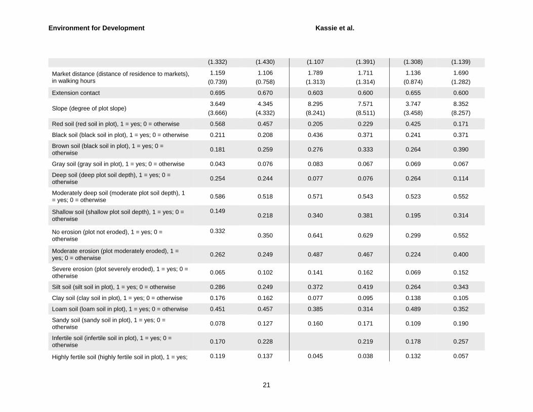
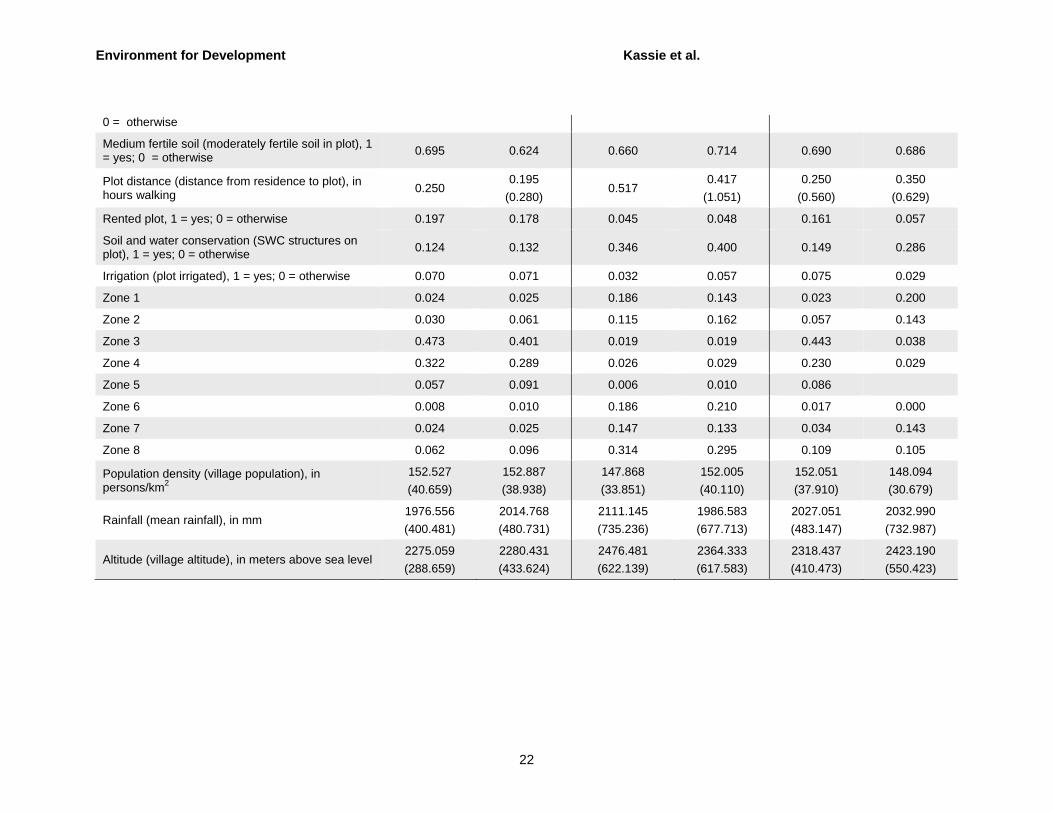
endogeneity bias could be addressed using the panel nature of our data and Mundlak’s approach (Wooldridge 2002). In addition, our rich plot and household characteristics dataset (tables 1 and 2 in the appendix) could assist in reducing both household and plot unobserved effects.
Controlling for the above econometric problems and incorporating equation (5) into equation (4), the expected yield difference between adoption and non-adoption of reduced tillage and/or chemical fertilizer becomes:
1 0 1 0 1 0( , , 1) ( , , 0) ( ) ( ).hp hp h hp hp hp h hp hpE y x u d E y x u d x xβ β γ γ= − = = − + −
(6)
The second term on the left-hand side of equation (6) is the expected value of y , if a plot
had not received reduced tillage or chemical fertilizer treatment. The difference between the expected outcome with and without the treatment, conditional on hpx , is our parameter of interest
in the parametric regression analysis. Equation (6) was also be estimated without including the second term of the right-hand side of the equation (i.e., without the Mundlak approach) for comparison purposes and to assess the robustness of the econometric results. It is important to note that the parametric analysis is based on observations that fell within common support from the propensity score matching process, i.e., matched observations.
2. Data and Descriptive Statistics
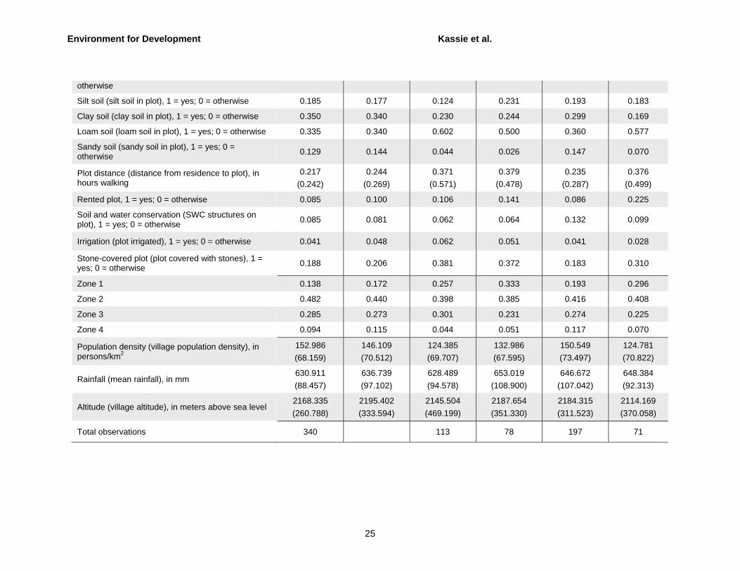
The data used in this study are from a farm survey conducted in 1999–2000 in the Tigray and Amhara regions of Ethiopia. Plots analyzed are located 1500 meters above sea level. The Amhara region dataset includes 435 farm households, 98 villages, 49 kebeles,2 and about 1365 plots, while the Tigray dataset include 500 farm households, 100 villages, 50 kebeles, and 1067 plots.3
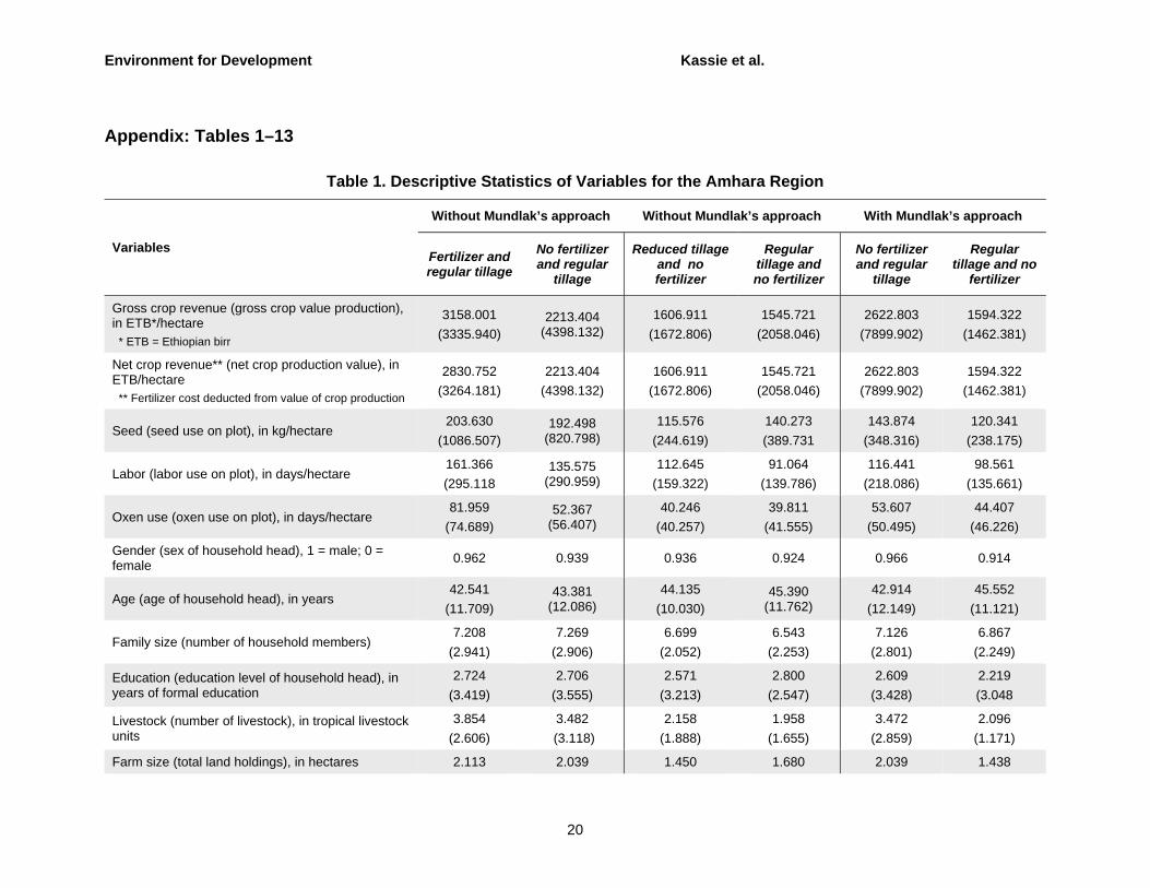
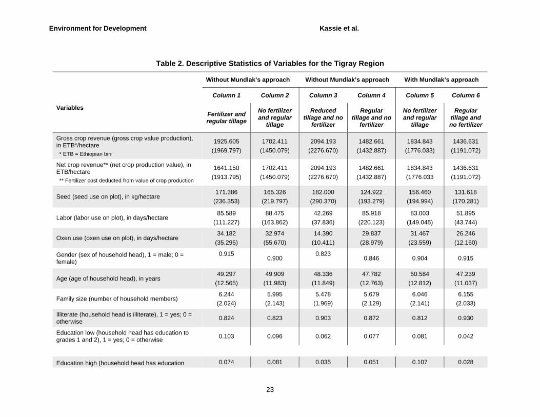
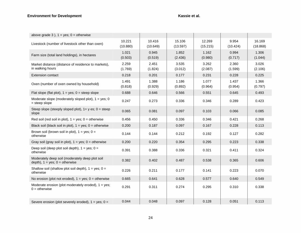
Tables 1 and 2 in the appendix present the descriptive statistics of variables used in the analysis by regions for the sub-samples of plots after matching. We conducted four comparisons to assess reduced tillage and fertilizer impact on productivity. These are 1) chemical fertilizer and regular tillage versus no fertilizer and regular tillage, 2) reduced tillage and no fertilizer versus regular tillage and no fertilizer, 3) reduced tillage and fertilizer versus reduced tillage and
2 A kebele is a higher administrative unit than a village and is often translated as “peasant association.” 3 For more details on study areas, sampling techniques, and criterions used to select sample areas, please see Pender and Gebremedhin (2006) and Benin (2006).
Environment for Development Kassie et al.
9
no fertilizer; and 4) reduced tillage and fertilizer versus regular tillage and fertilizer. Regular tillage is used here to refer to the normal or traditional tillage practices. Comparisons 1 and 3 enable assessing the impact of fertilizer under different tillage regimes, while comparisons 2 and 4 enable assessing impacts of tillage practices under different fertilizer use regimes. The last two comparisons have a small number of observations after matching. (See tables 1 and 2 in the appendix.) We did not present the descriptive statistics of these comparisons, but they are available upon request.
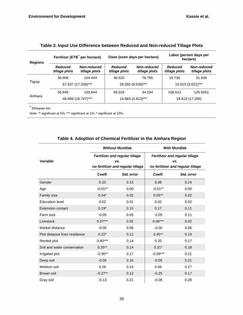
About 13.2 percent and 34.5 percent of the total sample plots in Tigray and 14.6 percent and 30.3 percent in Amhara region used reduced tillage and chemical fertilizer, respectively. The conditional mean fertilizer value (conditional being fertilizer use) was about ETB 2814 per hectare in Tigray and ETB 361 per hectare in Amhara. Production costs (labor, fertilizer, and oxen use) are lower on reduced tillage plots compared to non-reduced tillage plots. (See table 3 in the appendix.) This is the direct benefit of using sustainable agriculture practices.
The mean plot altitude, which was associated closely with temperature and microclimates, was 2175 and 2350 meters above sea level for Tigray and Amhara regions, respectively. The average annual rainfall in Amhara was about 1981 mm per year and 648 mm in the Tigray region,5 respectively. Rainfall in Amhara study sites, therefore, averaged approximately three times that of Tigray. Differences across the two regions are thus very large. The mean population density was 142 persons per square kilometer for Tigray and 158 for Amhara region.
In addition to these variables, several plot characteristics, household characteristics, endowments, and indicators of access to infrastructure were included in the empirical model. The choice of these variables was guided by economic theory and previous empirical research. Given missing and/or imperfect markets in Ethiopia, households’ initial resource endowments and characteristics were expected to play a role in investment and production decisions and were thus included in the analysis (Holden et al. 2001; Pender and Kerr 1998). The plot characteristics in the dataset included plot slope, position on slope, plot size, soil fertility, soil depth, soil color,
4 ETB = Ethipian birr. 5 The mean rainfall data are based long-term rainfall averages, spatially interpolated using a climate model (Corbett and White 2001). The minimum and maximum rainfall averaged over the Amhara region for the last 50 years (1953–2003) was 1303 and 2457 mm, respectively. Even the minimum average rainfall in Amhara is higher than the maximum annual rainfall (994 mm) of the drier region, Tigray.
Environment for Development Kassie et al.
10
soil textures, plot distance from homestead, and input use by plot. Including observed plot characteristics and inputs could also help address selection due to idiosyncratic errors, such as plot heterogeneity. Observable plot characteristics might be correlated with unobservable ones (Fafchamps 1993; Levinsohn and Petrin 2003; Assunção and Braido 2004). Including input use also helped control for plot heterogeneity because farmers typically respond to shocks (positive or negative) by changing input use (ibid.).
3. Empirical Results In this section, we present and discuss the empirical results, starting with results from
semi-parametric analysis and followed by results from parametric estimations.
3.1 Results from Semi-Parametric Analysis
As the foregoing discussion on the econometric strategy showed, the use of PSM allowed us to explore how the plot and household characteristics influenced the households’ decisions to adopt either reduced tillage or chemical fertilizer, as well as how the adoption subsequently impacted crop productivity. In particular, we used the PSM to compare the impact of reduced tillage and chemical fertilizer on crop productivity. We did this via several pair-wise comparisons. First, we compared the productivity of plots with chemical fertilizer and regular tillage to plots with regular tillage but no chemical fertilizer. Second, we compared plots with reduced tillage but no chemical fertilizer to plots with regular tillage but no chemical fertilizer. Third, plots with reduced tillage and chemical fertilizer were compared to plots with reduced tillage but no chemical fertilizer. Fourth, we considered plots with both reduced tillage and chemical fertilizer against plots with regular tillage and chemical fertilizer. Finally, we compared the productivity of plots with reduced tillage but no chemical fertilizer to plots with chemical fertilizer and regular tillage. This implies that our analysis 1) assessed the impacts of chemical fertilizer under different tillage regimes (achieved in the first and third comparisons), and 2) assessed impacts of tillage practices under different chemical fertilizer use regimes (achieved in the second and fourth comparisons). Thus, these comparisons enabled assessment of interactions between tillage regime and fertilizer use on productivity. Furthermore, by comparing the results from the two data sets, we were able to understand how agroecology affects productivity impacts.
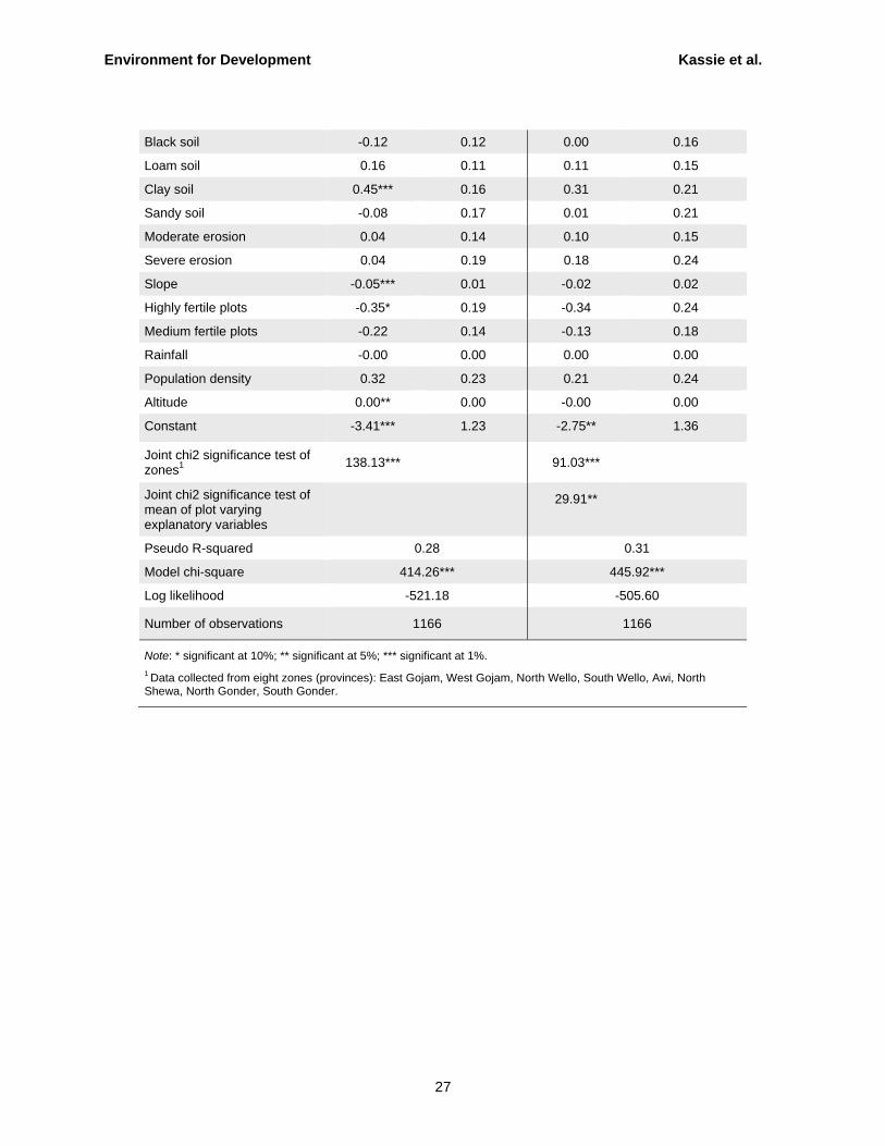
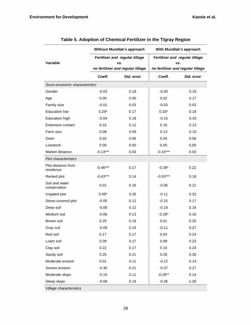
Tables 4, 5, 6, and 7 (in the appendix) present probit results of the above comparisons. The PSM was performed with and without Mundlak’s approach for comparison purposes, although the statistical evidence found in the correlation between observed explanatory variables

Environment for Development Kassie et al.
11
and unobserved effects suggests that ignoring this might lead to biased estimates. In the interest of space and because our main goal in the matching method is to identify the average treatment effect on the treated plots (ATT) and obtain matched treated and non-treated observations to use them as input for parametric regression, the score estimates are not discussed in detail, but the results along with the matching variables are reported in tables 4, 5, 6, and 7 in the appendix.
The results suggested that both socio-economic and plot characteristics were significant in conditioning the households’ decisions to adopt any technology. In addition, there was heterogeneity with regards to factors influencing the choice to adopt conservation tillage or chemical fertilizer.
Table 8 (see appendix) provides the nearest-neighbor matching method estimates. As mentioned earlier, we started by matching plots with chemical fertilizer and regular tillage to plots with regular tillage but no chemical fertilizer (model 1). Second, we matched the productivity impacts of reduced tillage with no chemical fertilizer to regular tillage with no chemical fertilizer (model 2). Third, plots with reduced tillage and chemical fertilizer were matched to plots with reduced tillage but no chemical fertilizer (model 3). Finally, we compared plots with both reduced tillage and chemical fertilizer to plots with regular tillage and chemical fertilizer (model 4). The results are reported for gross crop revenue per hectare.
The results revealed that using chemical fertilizer was more productive in the high-rainfall areas of the Amhara region, but it showed no significant crop productivity impact in the low-rainfall areas of the Tigray region.
6 On the other hand, reduced tillage was more productive
in the low rainfall areas of the Tigray region. However, it had no significant crop productivity impact in the high rainfall areas of the Amhara region. These results hold for all comparisons except for model 4.
7 Although the number of observations for models 3 and 4 is small and
impact of reduced tillage has insignificant impact in the Amhara region, it seems the productivity of reduced tillage can be increased by combining it with chemical fertilizer. This is because organic inputs are poor sources of some nutrients, especially phosphorus, and are often limited in availability to farmers (Palm et al. 1997, 193–217). This indicates that, in Tigray, reduced tillage leads to significantly higher productivity gains than chemical fertilizers. This result is consistent
6 The results are consistent in high-rainfall areas when net crop revenue are used, i.e., when the monetary cost of fertilizer has been deducted, but in low-rainfall areas, it turned out to be negative and insignificant. 7 This result is consistent with results using alternative matching methods, such as kernel and stratification matching methods.
Environment for Development Kassie et al.
12
with Pender and Gebremedhin (2008), who found that fertilizer use is not very profitable in arid environments.
The finding that sustainable agricultural practices enhance crop productivity is consistent with findings of previous research based on data from Tigray. For example, empirical results from a project on sustainable agriculture (the main activities were to implement sustainable agriculture practices, such as composting, water and soil conservation activities, and crop diversification), carried out since 1996 in the Tigray region in Ethiopia, demonstrate the superiority, in terms of its impact on productivity, of using compost compared to chemical fertilizer (Araya and Edwards 2006; Kassie et al. 2008b).
3.2 Results from Parametric Analysis
All regression models except for the control group (regular tillage and no fertilizer) in model 3 were estimated using random effects methods.8 Parametric regression was not run for models 3 and 4 because they had insufficient observations; the regression models turned out to be insignificant. Models 1 and 2 were estimated with and without Mundlak’s approach, although our statistical evidence indicated that the vectorγ is statistically different from zero, implying
that there is a correlation between observed regressors and unobserved random effects. The dependent variable in all cases was the gross crop revenue per hectare in natural logarithmic form. Our parameter of interest, as indicated in equation (6) is to estimate the ATT (difference in mean gross crop revenue per hectare) of conservation tillage and chemical fertilizer adoption. In the interest of brevity, we have not discussed the details of the estimated coefficients of the explanatory variables but these results are available in tables 9–12 in the appendix.
In brief, the results underscored the significance of plot and household characteristics, as well as conventional agricultural inputs (seeds, labor, and oxen),9 in influencing crop productivity. More importantly, the results suggested that the effectiveness of these factors in influencing crop productivity varies depending on the technology that has been adopted on a
8 The control group had insufficient observations to run random effects except pooled OLS. However, the same conclusion was reached when both treatment and control groups were run using pooled OLS. 9 Traditionally, farm households retain their own seeds from previous harvests for planting. Seed use is, therefore, a pre-determined variable. Improved seeds were used only on 3 percent and 1 percent of all sample plots in the Tigray and Amhara regions, respectively. We assumed labor and oxen use were fixed in the short term since households usually depend on family resources.
Environment for Development Kassie et al.
13
given plot. Thus, understanding how these factors interact with specific technology is crucial for policy makers as this will enable them to formulate more effective and appropriate polices.
The switching regression estimates from tables 9–12 (see appendix) were used to investigate the predicted gross crop revenue gap between plots with reduced tillage and no fertilizer versus regular tillage and no fertilizer and plots with fertilizer and regular tillage versus no fertilizer and regular tillage.
Consistent with results from the semi-parametric analysis, parametric results without Mundlak’s approach indicated that, while in both regions chemical fertilizer enhanced productivity, it leads to significantly higher productivity gains in the high-rainfall areas (table 13 in the appendix). However, using Mundlak’s approach, we found that chemical fertilizer had no significant productivity impact in low rainfall areas. Again, these results were robust to both gross and net crop revenue per hectare except for model 1 of low-rainfall areas where fertilizer is negative and insignificant.10 On the other hand, as in the semi-parametric regression results, reduced tillage had significant impact in the low-rainfall areas. However, this significance was not observed in the high-rainfall areas.
In sum, the empirical results showed that adoption of sustainable agricultural practices, such as reduced tillage, could create a win-win situation for resource-constrained farmers in a dry land environment, i.e., they can reduce production costs, promote environmental benefits, and, at the same time, lead to increased yields. Thus, promotion of sustainable agricultural practices could help increase agricultural productivity, as well as contribute to environmental benefits in low-rainfall areas of Ethiopia.
4. Conclusions and Policy Implications
Inadequate nutrient supply, depletion of soil organic matter, and soil erosion continue to present serious challenges to crop production in Ethiopia. This is further compounded by increased population pressure that is not accompanied by technological and/or efficiency progress. Efforts by the government to promote the adoption of chemical fertilizers have been frustrated by escalating fertilizer prices and production and consumption risks associated with fertilizer adoption. The efforts lack a clear understanding of the role of agroecology, such as rainfall, in conditioning the effectiveness of technology adoption to enhance productivity of
10 These results (not reported) were also robust after controlling for crop types.
Environment for Development Kassie et al.
14
agriculture, i.e., agroecology shapes the performance of technology. The distribution and amount of rainfall varies both in spatial and temporal terms across and within Ethiopia. This implies that the profitability of adopting sustainable agricultural practices, vis-à-vis chemical fertilizer, will depend on the distribution of rainfall (i.e., agroecology), and thus this should play a role when formulating policies that promote adoption of productivity-enhancing technologies, such as chemical fertilizer and reduced tillage.
In this paper, we examined the productivity gains associated with adoption of sustainable agricultural practices, with a particular focus on adoption of reduced tillage. We also investigated how these productivity gains compared to the gain resulting from chemical fertilizer use. To do so, we employed two sets of plot-level data from Ethiopia: one from a low-rainfall area in the Tigray region and another from a high-rainfall area in the Amhara region. This nature of the data allowed us to further examined whether agroecology, defined here with reference to rainfall abundance, influences the productivity gains associated with the reduced tillage and chemical fertilizer. To do so, we employed both semi-parametric and parametric econometric methods which permitted us to (1) explore how household and plot characteristics influence decisions to adopt either reduced tillage or chemical fertilizer, (2) assess the impact of these technologies on crop productivity, and (3) explore determinants of crop production in general. Interestingly, our results revealed a clear superiority of reduced tillage over chemical fertilizers in enhancing crop productivity in the low-rainfall region. In the high-rainfall region, however, chemical fertilizer is overwhelmingly superior and reduced tillage potentially results in productivity losses in some cases.
The results thus suggest that the promotion of farming technologies should not be based on policies that fail to incorporate the impact of agroecology on both adoption decisions, as well as the profitability of the technology in question. As the results showed, while sustainable agricultural practices such as reduced tillage can help increase agricultural productivity in semi-arid contexts (such as the Tigray region of Ethiopia), it had no impact on productivity in the high-rainfall Amhara region. Chemical fertilizer had a large and significant impact in the high-rainfall Amhara region. The productivity advantages of reduced tillage may derive from conservation of soil moisture in dry environments, where inorganic fertilizer use is less profitable and risky due to inadequate soil moisture. There is a need for governments and non-governmental organizations to shift their focus from chemical fertilizers to considering sustainable agricultural practices as yield-augmenting technologies in semi-arid and arid areas. In these areas, sustainable agricultural practices not only increase yields but could also provide other benefits: farmers may also be able to cut production costs, increase environmental benefits,

Environment for Development Kassie et al.
15
reduce crop failure risk due to moisture stress, and decrease financial risk associated with buying chemical fertilizer on credit.
Environment for Development Kassie et al.
16
References
Adesina, A.A., D. Mbila, G.B. Nkamleu, and D. Endamana. 2000. “Econometric Analysis of the Determinants of Adoption of Alley Farming by Farmers in the Forest Zone of Southwest Cameroon,”Agriculture, Ecoystems and Environment 80: 255–65.
Araya, H., and S. Edwards. 2006. The Tigray Experience: A Success Story in Sustainable Agriculture. Third World Network (TWN) Environment and Development Series 4. Penang, Malaysia: TWN.
Assunção, J.J., and B.H.L. Braido. 2004. “Testing among Competing Explanations for the Inverse Productivity Puzzle.” Unpublished paper. http://www.econ.puc-rio.br/PDF/seminario/2004/inverse.pdf. Accessed April 2009.
Benin, S. 2006. “Policies and Programs Affecting Land Management Practices, Input Use, and Productivity in the Highlands of Amhara Region, Ethiopia.” In Strategies for Sustainable Land Management in the East African Highlands, edited by J. Pender, F. Place, and S. Ehui. Washington, DC: IFPRI.
Byerlee, D., D.J. Spielman, D. Alemu, and M. Gautam. 2007. “Policies to Promote Cereal Intensification in Ethiopia: A Review of Evidence and Experience.” International Food Policy Research Institute Discussion Paper, no. 00707. Washington, DC: IFPRI.
Caviglia, J.L., and J.R. Kahn. 2001. “Diffusion of Sustainable Agriculture in the Brazilian Rain Forest: A Discrete Choice Analysis,” Economic Development and Cultural Change 49: 311–33.
Dercon, S., and L. Christiaensen. 2007. “Consumption Risk, Technology Adoption and Poverty Traps: Evidence from Ethiopia.” World Bank Policy Research Working Paper 4527. Washington, DC: World Bank.
Edwards, S., A. Asmelash, H. Araya, and T.B. Gebre-Egziabher. 2007. Impact of Compost Use on Crop Production in Tigary, Ethiopia.” Rome: FAO, Natural Resources Management and Environment Department.
EEA/EEPRI (Ethiopian Economic Association/Ethiopian Economic Policy Research Institute). 2006. “Evaluation of the Ethiopian Agricultural Extension with Particular Emphasis on the Participatory Demonstration and Training Extension System (PADETES).” Addis Ababa, Ethiopia: EEA/EEPRI.
Environment for Development Kassie et al.
17
Fafchamps, M. 1993. “Sequential Labour Decisions under Uncertainty: An Estimable Household Model of West Africa Farmers,” Econometrica 61: 1173–97.
Food and Agriculture Organization (FAO). 2008. Web site. “Conservation Agriculture.” http://www.fao.org/ag/ca/. Accessed April 2009.
Fischer T., N. Turner, J. Angus, L. McIntyre, M. Robertson, A. Borrell, and D. Lloyd. 2004. “New Directions for a Diverse Planet: Proceedings of the 4th International Crop Science Congress,” Brisbane, Australia, 26 September–1 October 2004.
Grepperud, S. 1996. “Population Pressure and Land Degradation: The Case of Ethiopia,” Journal of Environmental Economics and Management 30: 18–33.
Holden, S.T., B. Shiferaw, and J. Pender. 2001. “Market Imperfections and Profitability of Land Use in the Ethiopian Highlands: A Comparison of Selection Models with Heteroskedasticity,” Journal of Agricultural Economics 52(2): 53–70.
Honlonkou, A.N. 2004. “Modelling Adoption of Natural Resources Management Technologies: The Case of Fallow Systems,” Environment and Development Economics 9: 289–314.
Kassie, M., J. Pender, M. Yesuf, G. Köhlin, R. Bluffstone, and E. Mulugeta. 2008a. “Estimating Returns to Soil Conservation Adoption in the Northern Ethiopian Highlands,” Agricultural Economics 38: 213–32.
Kassie, M., M. Yesuf, and G. Köhlin. 2008. “The Role of Production Risk in Sustainable Land-Management Technology Adoption in the Ethiopian Highlands.” EfD Discussion Paper 08-15. Washington, DC: Resources for the Future.
Kassie, M., P. Zikhali, K. Manjur, and S. Edwards. 2008b. “Adoption of Organic Farming Technologies: Evidence from Semi-arid Regions of Ethiopia.” Scandinavian Working Papers in Economics, no. 335. Gothenburg, Sweden: University of Gothenburg, Department of Economics. http://swopec.hhs.se/gunwpe/abs/gunwpe0335.htm. Accessed April 2009.
Kassie, M., and T.S. Holden. 2006. ”Parametric and Non-parametric Estimation of Soil Conservation Adoption Impact on Productivity in the Northwestern Ethiopian Highlands.” Paper presented at the International Association of Agricultural Economists Conference, Gold Coast, Australia, August 12–18, 2006. http://ageconsearch.umn.edu/bitstream/25281/1/cp060544.pdf. Accessed April 2009.
Environment for Development Kassie et al.
18
Lee, D.R. 2005. “Agricultural Sustainability and Technology Adoption: Issues and Policies for Developing Countries,” American Journal of Agricultural Economics 87(5): 1325–34.
Levinsohn, J., and A. Petrin. 2003. “Estimating Production Functions Using Inputs to Control for Unobservable,” Review of Economic Studies 70: 317–41.
Mundlak, Y. 1978. “On the Pooling of Time Series and Cross Section Data,” Econometrica 64(1): 69–85.
Palm, C.A., R.J.K. Myers, and S.N. Nandwa. 1997. “Combined Use of Organic and Inorganic Nutrient Sources for Soil Fertility Maintenance and Replenishment.” In Replenishing Soil Fertility in Africa, edited by R. J. Buresh, P.A. Sanchez, and F. Calhoun. SSSA Special Publication 51. Madison, WI, USA: Soil Science Socity of America and American Society of Agronomy. http://www.worldagroforestry.org/units/Library/Books/PDFs/91_Replenishing_soil_fertility_in_africa.pdf. Accessed April 2009.
Pender, J., and B. Gebremedhin. 2006. “Land Management, Crop Production, and Household Income in the Highlands of Tigray, Northern Ethiopia: An Econometric Analysis. In Strategies for Sustainable Land Management in the East African Highlands, edited by J. Pender, F. Place, and S.Ehui. Washington, DC: IFPRI.
Pender, J., and J.M. Kerr. 1998. ”Determinants of Farmer’s Indigenous Soil And Water Conservation Investments In Semi-Arid India,” Agricultural Economics 19, 113–25.
Place, F., and P. Dewees. 1999. “Policies and Incentives for the Adoption of Improved Fallows,” Agroforestry Systems 47: 323–43.
Rosenbaum, P.R., and D.B. Rubin. 1983. “The Central Role of the Propensity Score in Observational Studies for Causal Effects,” Biometrika 70(1), 41–55.
Sasakawa Africa Association. 2008. Web site. “Country Profile: Ethiopia.” http://www.saa-tokyo.org/english/country/ethiopia.shtml. Accessed April 2009.
Shiferaw, B., and S.T. Holden. 1998. “Resource Degradation and Adoption of Land Conservation Technologies in the Ethiopian Highlands: A Case Study in Andit Tid, North Shewa,” Agricultural Economics 18: 233–47.
Sutcliffe, J.P. 1993. “Economic Assessment of Land Degradation in the Ethiopian Highlands: A Case Study.” Addis Ababa, Ethiopia: Transitional Government of Ethiopia, Ministry of Planning and Economic Development, National Conservation Strategy Secretariat.
Environment for Development Kassie et al.
19
Twarog. 2006. “Organic Agriculture: A Trade and Sustainable Development Opportunity for Developing Countries.” In Trade and Environment Review 2006. New York and Geneva: UN/UNCTAD. http://www.unctad.org/en/docs/ditcted200512_en.pdf. Accessed April 2009.
Wooldridge, J.M., 2002. Econometric Analysis of Cross Section and Panel Data. 1st ed. Cambridge, MA, USA: MIT Press.
World Bank. 2005. World Development Indicators 2005. Database. http://devdata.worldbank.org/wdi2005/Section2.htm. Accessed April 2009.
———. 2007. World Development Report 2008: Agriculture for Development. Washington, DC: World Bank.
Environment for Development Kassie et al.
20
Appendix: Tables 1–13
Table 1. Descriptive Statistics of Variables for the Amhara Region
Variables
Without Mundlak’s approach Without Mundlak’s approach With Mundlak’s approach
Fertilizer and regular tillage
No fertilizer and regular
tillage
Reduced tillage and no fertilizer
Regular tillage and no fertilizer
No fertilizer and regular
tillage
Regular tillage and no
fertilizer
Gross crop revenue (gross crop value production), in ETB*/hectare * ETB = Ethiopian birr
3158.001 (3335.940)
2213.404 (4398.132)
1606.911 (1672.806)
1545.721 (2058.046)
2622.803 (7899.902)
1594.322 (1462.381)
Net crop revenue** (net crop production value), in ETB/hectare ** Fertilizer cost deducted from value of crop production
2830.752 (3264.181)
2213.404 (4398.132)
1606.911 (1672.806)
1545.721 (2058.046)
2622.803 (7899.902)
1594.322 (1462.381)
Seed (seed use on plot), in kg/hectare 203.630
(1086.507) 192.498
(820.798) 115.576
(244.619) 140.273 (389.731
143.874 (348.316)
120.341 (238.175)
Labor (labor use on plot), in days/hectare 161.366 (295.118
135.575 (290.959)
112.645 (159.322)
91.064 (139.786)
116.441 (218.086)
98.561 (135.661)
Oxen use (oxen use on plot), in days/hectare 81.959
(74.689) 52.367
(56.407) 40.246
(40.257) 39.811
(41.555) 53.607
(50.495) 44.407
(46.226)
Gender (sex of household head), 1 = male; 0 = female 0.962 0.939 0.936 0.924 0.966 0.914
Age (age of household head), in years 42.541
(11.709) 43.381
(12.086) 44.135
(10.030) 45.390
(11.762) 42.914
(12.149) 45.552
(11.121)
Family size (number of household members) 7.208
(2.941) 7.269
(2.906) 6.699
(2.052) 6.543
(2.253) 7.126
(2.801) 6.867
(2.249)
Education (education level of household head), in years of formal education
2.724 (3.419)
2.706 (3.555)
2.571 (3.213)
2.800 (2.547)
2.609 (3.428)
2.219 (3.048
Livestock (number of livestock), in tropical livestock units
3.854 (2.606)
3.482 (3.118)
2.158 (1.888)
1.958 (1.655)
3.472 (2.859)
2.096 (1.171)
Farm size (total land holdings), in hectares 2.113 2.039 1.450 1.680 2.039 1.438
Environment for Development Kassie et al.
21
(1.332) (1.430) (1.107 (1.391) (1.308) (1.139)
Market distance (distance of residence to markets), in walking hours
1.159 (0.739)
1.106 (0.758)
1.789 (1.313)
1.711 (1.314)
1.136 (0.874)
1.690 (1.282)
Extension contact 0.695 0.670 0.603 0.600 0.655 0.600
Slope (degree of plot slope) 3.649
(3.666) 4.345
(4.332) 8.295
(8.241) 7.571
(8.511) 3.747
(3.458) 8.352
(8.257)
Red soil (red soil in plot), 1 = yes; 0 = otherwise 0.568 0.457 0.205 0.229 0.425 0.171
Black soil (black soil in plot), 1 = yes; 0 = otherwise 0.211 0.208 0.436 0.371 0.241 0.371
Brown soil (black soil in plot), 1 = yes; 0 = otherwise 0.181 0.259 0.276 0.333 0.264 0.390
Gray soil (gray soil in plot), 1 = yes; 0 = otherwise 0.043 0.076 0.083 0.067 0.069 0.067
Deep soil (deep plot soil depth), 1 = yes; 0 = otherwise 0.254 0.244 0.077 0.076 0.264 0.114
Moderately deep soil (moderate plot soil depth), 1 = yes; 0 = otherwise 0.586 0.518 0.571 0.543 0.523 0.552
Shallow soil (shallow plot soil depth), 1 = yes; 0 = otherwise
0.149
0.218 0.340 0.381 0.195 0.314
No erosion (plot not eroded), 1 = yes; 0 = otherwise
0.332
0.350 0.641 0.629 0.299 0.552
Moderate erosion (plot moderately eroded), 1 = yes; 0 = otherwise 0.262 0.249 0.487 0.467 0.224 0.400
Severe erosion (plot severely eroded), 1 = yes; 0 = otherwise 0.065 0.102 0.141 0.162 0.069 0.152
Silt soil (silt soil in plot), 1 = yes; 0 = otherwise 0.286 0.249 0.372 0.419 0.264 0.343
Clay soil (clay soil in plot), 1 = yes; 0 = otherwise 0.176 0.162 0.077 0.095 0.138 0.105
Loam soil (loam soil in plot), 1 = yes; 0 = otherwise 0.451 0.457 0.385 0.314 0.489 0.352
Sandy soil (sandy soil in plot), 1 = yes; 0 = otherwise 0.078 0.127 0.160 0.171 0.109 0.190
Infertile soil (infertile soil in plot), 1 = yes; 0 = otherwise 0.170 0.228 0.219 0.178 0.257
Highly fertile soil (highly fertile soil in plot), 1 = yes; 0.119 0.137 0.045 0.038 0.132 0.057
Environment for Development Kassie et al.
22
0 = otherwise
Medium fertile soil (moderately fertile soil in plot), 1 = yes; 0 = otherwise 0.695 0.624 0.660 0.714 0.690 0.686
Plot distance (distance from residence to plot), in hours walking 0.250
0.195 (0.280)
0.517 0.417
(1.051) 0.250
(0.560) 0.350
(0.629)
Rented plot, 1 = yes; 0 = otherwise 0.197 0.178 0.045 0.048 0.161 0.057
Soil and water conservation (SWC structures on plot), 1 = yes; 0 = otherwise 0.124 0.132 0.346 0.400 0.149 0.286
Irrigation (plot irrigated), 1 = yes; 0 = otherwise 0.070 0.071 0.032 0.057 0.075 0.029
Zone 1 0.024 0.025 0.186 0.143 0.023 0.200
Zone 2 0.030 0.061 0.115 0.162 0.057 0.143
Zone 3 0.473 0.401 0.019 0.019 0.443 0.038
Zone 4 0.322 0.289 0.026 0.029 0.230 0.029
Zone 5 0.057 0.091 0.006 0.010 0.086
Zone 6 0.008 0.010 0.186 0.210 0.017 0.000
Zone 7 0.024 0.025 0.147 0.133 0.034 0.143
Zone 8 0.062 0.096 0.314 0.295 0.109 0.105
Population density (village population), in persons/km2
152.527 (40.659)
152.887 (38.938)
147.868 (33.851)
152.005 (40.110)
152.051 (37.910)
148.094 (30.679)
Rainfall (mean rainfall), in mm 1976.556 (400.481)
2014.768 (480.731)
2111.145 (735.236)
1986.583 (677.713)
2027.051 (483.147)
2032.990 (732.987)
Altitude (village altitude), in meters above sea level 2275.059 (288.659)
2280.431 (433.624)
2476.481 (622.139)
2364.333 (617.583)
2318.437 (410.473)
2423.190 (550.423)
Environment for Development Kassie et al.
23
Table 2. Descriptive Statistics of Variables for the Tigray Region
Variables
Without Mundlak’s approach Without Mundlak’s approach With Mundlak’s approach
Column 1 Column 2 Column 3 Column 4 Column 5 Column 6
Fertilizer and regular tillage
No fertilizer and regular
tillage
Reduced tillage and no
fertilizer
Regular tillage and no
fertilizer
No fertilizer and regular
tillage
Regular tillage and no fertilizer
Gross crop revenue (gross crop value production), in ETB*/hectare * ETB = Ethiopian birr
1925.605 (1969.797)
1702.411 (1450.079)
2094.193 (2276.670)
1482.661 (1432.887)
1834.843 (1776.033)
1436.631 (1191.072)
Net crop revenue** (net crop production value), in ETB/hectare ** Fertilizer cost deducted from value of crop production
1641.150 (1913.795)
1702.411 (1450.079)
2094.193 (2276.670)
1482.661 (1432.887)
1834.843 (1776.033
1436.631 (1191.072)
Seed (seed use on plot), in kg/hectare 171.386
(236.353) 165.326
(219.797) 182.000
(290.370) 124.922
(193.279) 156.460
(194.994) 131.618
(170.281)
Labor (labor use on plot), in days/hectare 85.589
(111.227) 88.475
(163.862) 42.269
(37.836) 85.918
(220.123) 83.003
(149.045) 51.895
(43.744)
Oxen use (oxen use on plot), in days/hectare 34.182
(35.295) 32.974
(55.670) 14.390
(10.411) 29.837
(28.979) 31.467
(23.559) 26.246
(12.160)
Gender (sex of household head), 1 = male; 0 = female)
0.915
0.900 0.823
0.846 0.904 0.915
Age (age of household head), in years 49.297
(12.565) 49.909
(11.983) 48.336
(11.849) 47.782
(12.763) 50.584
(12.812) 47.239
(11.037)
Family size (number of household members) 6.244
(2.024) 5.995
(2.143) 5.478
(1.969) 5.679
(2.129) 6.046
(2.141) 6.155
(2.033)
Illiterate (household head is illiterate), 1 = yes; 0 = otherwise 0.824 0.823 0.903 0.872 0.812 0.930
Education low (household head has education to grades 1 and 2), 1 = yes; 0 = otherwise 0.103 0.096 0.062 0.077 0.081 0.042
Education high (household head has education 0.074 0.081 0.035 0.051 0.107 0.028
Environment for Development Kassie et al.
24
above grade 3 ), 1 = yes; 0 = otherwise
Livestock (number of livestock other than oxen) 10.221
(10.880) 10.416
(10.649) 15.106
(13.597) 12.269
(15.215) 9.954
(10.424) 16.169
(18.868)
Farm size (total land holdings), in hectares 1.021
(0.503) 0.945
(0.519) 1.852
(2.436) 1.162
(0.980) 0.994
(0.717) 1.306
(1.044)
Market distance (distance of residence to markets), in walking hours
2.259 (1.769)
2.451 (1.824)
3.535 (3.012)
3.262 (2.087)
2.360 (1.599)
3.026 (2.106)
Extension contact 0.218 0.201 0.177 0.231 0.228 0.225
Oxen (number of oxen owned by household) 1.491
(0.818) 1.388
(0.929) 1.186
(0.892) 1.077
(0.964) 1.437
(0.954) 1.366
(0.797)
Flat slope (flat plot), 1 = yes; 0 = steep slope 0.688 0.646 0.566 0.551 0.645 0.493
Moderate slope (moderately sloped plot), 1 = yes; 0 = steep slope 0.247 0.273 0.336 0.346 0.289 0.423
Steep slope (steeply sloped plot), 1= y es; 0 = steep slope 0.065 0.081 0.097 0.103 0.066 0.085
Red soil (red soil in plot), 1 = yes; 0 = otherwise 0.456 0.450 0.336 0.346 0.421 0.268
Black soil (black soil in plot), 1 = yes; 0 = otherwise 0.200 0.187 0.097 0.167 0.228 0.113
Brown soil (brown soil in plot), 1 = yes; 0 = otherwise 0.144 0.144 0.212 0.192 0.127 0.282
Gray soil (gray soil in plot), 1 = yes; 0 = otherwise 0.200 0.220 0.354 0.295 0.223 0.338
Deep soil (deep plot soil depth), 1 = yes; 0 = otherwise 0.391 0.388 0.336 0.321 0.411 0.324
Moderately deep soil (moderately deep plot soil depth), 1 = yes; 0 = otherwise 0.382 0.402 0.487 0.538 0.365 0.606
Shallow soil (shallow plot soil depth), 1 = yes; 0 = otherwise 0.226 0.211 0.177 0.141 0.223 0.070
No erosion (plot not eroded), 1 = yes; 0 = otherwise 0.665 0.641 0.628 0.577 0.640 0.549
Moderate erosion (plot moderately eroded), 1 = yes; 0 = otherwise 0.291 0.311 0.274 0.295 0.310 0.338
Severe erosion (plot severely eroded), 1 = yes; 0 = 0.044 0.048 0.097 0.128 0.051 0.113
Environment for Development Kassie et al.
25
otherwise
Silt soil (silt soil in plot), 1 = yes; 0 = otherwise 0.185 0.177 0.124 0.231 0.193 0.183
Clay soil (clay soil in plot), 1 = yes; 0 = otherwise 0.350 0.340 0.230 0.244 0.299 0.169
Loam soil (loam soil in plot), 1 = yes; 0 = otherwise 0.335 0.340 0.602 0.500 0.360 0.577
Sandy soil (sandy soil in plot), 1 = yes; 0 = otherwise 0.129 0.144 0.044 0.026 0.147 0.070
Plot distance (distance from residence to plot), in hours walking
0.217 (0.242)
0.244 (0.269)
0.371 (0.571)
0.379 (0.478)
0.235 (0.287)
0.376 (0.499)
Rented plot, 1 = yes; 0 = otherwise 0.085 0.100 0.106 0.141 0.086 0.225
Soil and water conservation (SWC structures on plot), 1 = yes; 0 = otherwise 0.085 0.081 0.062 0.064 0.132 0.099
Irrigation (plot irrigated), 1 = yes; 0 = otherwise 0.041 0.048 0.062 0.051 0.041 0.028
Stone-covered plot (plot covered with stones), 1 = yes; 0 = otherwise 0.188 0.206 0.381 0.372 0.183 0.310
Zone 1 0.138 0.172 0.257 0.333 0.193 0.296
Zone 2 0.482 0.440 0.398 0.385 0.416 0.408
Zone 3 0.285 0.273 0.301 0.231 0.274 0.225
Zone 4 0.094 0.115 0.044 0.051 0.117 0.070
Population density (village population density), in persons/km2
152.986 (68.159)
146.109 (70.512)
124.385 (69.707)
132.986 (67.595)
150.549 (73.497)
124.781 (70.822)
Rainfall (mean rainfall), in mm 630.911 (88.457)
636.739 (97.102)
628.489 (94.578)
653.019 (108.900)
646.672 (107.042)
648.384 (92.313)
Altitude (village altitude), in meters above sea level 2168.335 (260.788)
2195.402 (333.594)
2145.504 (469.199)
2187.654 (351.330)
2184.315 (311.523)
2114.169 (370.058)
Total observations 340 113 78 197 71
Environment for Development Kassie et al.
26
Table 3. Input Use Difference between Reduced and Non-reduced Tillage Plots
Regions Fertilizer (ETB¤ per hectare) Oxen (oxen days per hectare) Labor (person days per
hectare)
Reduced tillage plots
Non-reduced tillage plots
Reduced tillage plots
Non-reduced tillage plots
Reduced tillage plots
Non-reduced tillage plots
Tigray 36.906 104.444 48.520 76.785 15.730 31.645
67.537 (17.209)*** 28.265 (9.539)*** 15.915 (3.021)***
Amhara 56.845 103.844 59.018 44.034 106.513 125.9261
46.999 (16.747)*** 14.983 (4.913)*** 19.413 (17.295)
¤ Ethiopian birr Note: ** significant at 5%; *** significant at 1%; * significant at 10%.
Table 4. Adoption of Chemical Fertilizer in the Amhara Region
Variable
Without Mundlak With Mundlak
Fertilizer and regular tillage vs.
no fertilizer and regular tillage
Fertilizer and regular tillage vs.
no fertilizer and regular tillage
Coeff. Std. error Coeff. Std. error
Gender 0.10 0.23 0.08 0.24
Age -0.01** 0.00 -0.01** 0.00
Family size 0.04* 0.02 0.05** 0.02
Education level 0.02 0.01 0.02 0.02
Extension contact 0.19* 0.10 0.17 0.11
Farm size -0.05 0.05 -0.05 0.11
Livestock 0.07*** 0.02 0.06*** 0.02
Market distance -0.00 0.06 -0.00 0.06
Plot distance from residence 0.22* 0.12 0.45** 0.19
Rented plot 0.40*** 0.14 0.20 0.17
Soil and water conservation 0.35** 0.14 0.31* 0.18
Irrigated plot -0.36** 0.17 -0.59*** 0.21
Deep soil -0.05 0.16 -0.05 0.21
Medium soil 0.16 0.14 0.06 0.17
Brown soil -0.27** 0.12 -0.25 0.17
Gray soil -0.13 0.21 -0.08 0.28
Environment for Development Kassie et al.
27
Black soil -0.12 0.12 0.00 0.16
Loam soil 0.16 0.11 0.11 0.15
Clay soil 0.45*** 0.16 0.31 0.21
Sandy soil -0.08 0.17 0.01 0.21
Moderate erosion 0.04 0.14 0.10 0.15
Severe erosion 0.04 0.19 0.18 0.24
Slope -0.05*** 0.01 -0.02 0.02
Highly fertile plots -0.35* 0.19 -0.34 0.24
Medium fertile plots -0.22 0.14 -0.13 0.18
Rainfall -0.00 0.00 0.00 0.00
Population density 0.32 0.23 0.21 0.24
Altitude 0.00** 0.00 -0.00 0.00
Constant -3.41*** 1.23 -2.75** 1.36
Joint chi2 significance test of zones1 138.13*** 91.03***
Joint chi2 significance test of mean of plot varying explanatory variables
29.91**
Pseudo R-squared 0.28 0.31
Model chi-square 414.26*** 445.92***
Log likelihood -521.18 -505.60
Number of observations 1166 1166
Note: * significant at 10%; ** significant at 5%; *** significant at 1%. 1 Data collected from eight zones (provinces): East Gojam, West Gojam, North Wello, South Wello, Awi, North Shewa, North Gonder, South Gonder.
Environment for Development Kassie et al.
28
Table 5. Adoption of Chemical Fertilizer in the Tigray Region
Variable
Without Mundlak’s approach With Mundlak’s approach
Fertilizer and regular tillage vs.
no fertilizer and regular tillage
Fertilizer and regular tillage vs.
no fertilizer and regular tillage
Coeff. Std. error Coeff. Std. error
Socio-economic characteristics
Gender -0.03 0.18 -0.00 0.19
Age 0.00 0.00 0.02 0.17
Family size -0.01 0.03 -0.03 0.03
Education low 0.29* 0.17 0.33* 0.18
Education high -0.04 0.18 -0.15 0.19
Extension contact 0.16 0.12 0.16 0.13
Farm size 0.08 0.09 0.13 0.10
Oxen 0.02 0.06 0.04 0.06
Livestock 0.00 0.00 0.00 0.00
Market distance -0.13*** 0.03 -0.15*** 0.03
Plot characteristics
Plot distance from residence -0.46*** 0.17 -0.39* 0.22
Rented plot -0.43*** 0.14 -0.53*** 0.18
Soil and water conservation 0.01 0.16 -0.06 0.21
Irrigated plot 0.49* 0.26 -0.11 0.32
Stone-covered plot -0.05 0.12 -0.15 0.17
Deep soil -0.09 0.12 -0.19 0.16
Medium soil -0.06 0.13 -0.28* 0.16
Brown soil 0.25 0.19 0.01 0.25
Gray soil -0.09 0.19 -0.11 0.27
Red soil 0.17 0.17 0.04 0.24
Loam soil 0.08 0.17 0.09 0.23
Clay soil 0.22 0.17 0.10 0.24
Sandy soil 0.25 0.21 0.28 0.30
Moderate erosion 0.01 0.11 -0.12 0.14
Severe erosion -0.30 0.21 -0.37 0.27
Moderate slope -0.16 0.11 -0.29** 0.14
Steep slope -0.08 0.19 -0.26 o.26
Village characteristics

Environment for Development Kassie et al.
29
Rainfall 0.15 0.55 0.65 0.58
Population density 0.02 0.12 0.00 0.00
Altitude -0.77* 0.43 -1.24*** 0.46
Constant 4.30 4.86 4.17 5.14
Joint chi2 significance test of zones1 23.72*** 19.19***
Joint chi2 significance test of mean of plot varying explanatory variables
30.83**
Pseudo R-squared 0.11 0.14
Model chi-square 139.41*** 171.28***
Log likelihood -539.08 -523.14
Number of observations 926 926
Note: * significant at 10%; ** significant at 5%; *** significant at 1%. 1 Data collected from four zones (provinces): southern, central, eastern, and western Tigray.
Environment for Development Kassie, Zikhali, Pender, and Köhlin
30
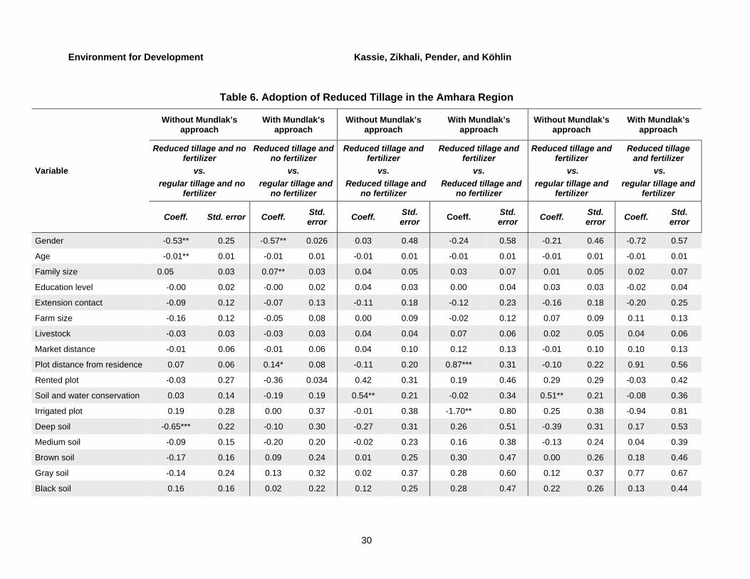
Table 6. Adoption of Reduced Tillage in the Amhara Region
Variable
Without Mundlak’s approach
With Mundlak’s approach
Without Mundlak’s approach
With Mundlak’s approach
Without Mundlak’s approach
With Mundlak’s approach
Reduced tillage and no fertilizer
vs. regular tillage and no
fertilizer
Reduced tillage and no fertilizer
vs. regular tillage and
no fertilizer
Reduced tillage and fertilizer
vs. Reduced tillage and
no fertilizer
Reduced tillage and fertilizer
vs. Reduced tillage and
no fertilizer
Reduced tillage and fertilizer
vs. regular tillage and
fertilizer
Reduced tillage and fertilizer
vs. regular tillage and
fertilizer
Coeff. Std. error Coeff. Std. error Coeff. Std.
error Coeff. Std. error Coeff. Std.
error Coeff. Std. error
Gender -0.53** 0.25 -0.57** 0.026 0.03 0.48 -0.24 0.58 -0.21 0.46 -0.72 0.57
Age -0.01** 0.01 -0.01 0.01 -0.01 0.01 -0.01 0.01 -0.01 0.01 -0.01 0.01
Family size 0.05 0.03 0.07** 0.03 0.04 0.05 0.03 0.07 0.01 0.05 0.02 0.07
Education level -0.00 0.02 -0.00 0.02 0.04 0.03 0.00 0.04 0.03 0.03 -0.02 0.04
Extension contact -0.09 0.12 -0.07 0.13 -0.11 0.18 -0.12 0.23 -0.16 0.18 -0.20 0.25
Farm size -0.16 0.12 -0.05 0.08 0.00 0.09 -0.02 0.12 0.07 0.09 0.11 0.13
Livestock -0.03 0.03 -0.03 0.03 0.04 0.04 0.07 0.06 0.02 0.05 0.04 0.06
Market distance -0.01 0.06 -0.01 0.06 0.04 0.10 0.12 0.13 -0.01 0.10 0.10 0.13
Plot distance from residence 0.07 0.06 0.14* 0.08 -0.11 0.20 0.87*** 0.31 -0.10 0.22 0.91 0.56
Rented plot -0.03 0.27 -0.36 0.034 0.42 0.31 0.19 0.46 0.29 0.29 -0.03 0.42
Soil and water conservation 0.03 0.14 -0.19 0.19 0.54** 0.21 -0.02 0.34 0.51** 0.21 -0.08 0.36
Irrigated plot 0.19 0.28 0.00 0.37 -0.01 0.38 -1.70** 0.80 0.25 0.38 -0.94 0.81
Deep soil -0.65*** 0.22 -0.10 0.30 -0.27 0.31 0.26 0.51 -0.39 0.31 0.17 0.53
Medium soil -0.09 0.15 -0.20 0.20 -0.02 0.23 0.16 0.38 -0.13 0.24 0.04 0.39
Brown soil -0.17 0.16 0.09 0.24 0.01 0.25 0.30 0.47 0.00 0.26 0.18 0.46
Gray soil -0.14 0.24 0.13 0.32 0.02 0.37 0.28 0.60 0.12 0.37 0.77 0.67
Black soil 0.16 0.16 0.02 0.22 0.12 0.25 0.28 0.47 0.22 0.26 0.13 0.44
Environment for Development Kassie, Zikhali, Pender, and Köhlin
31
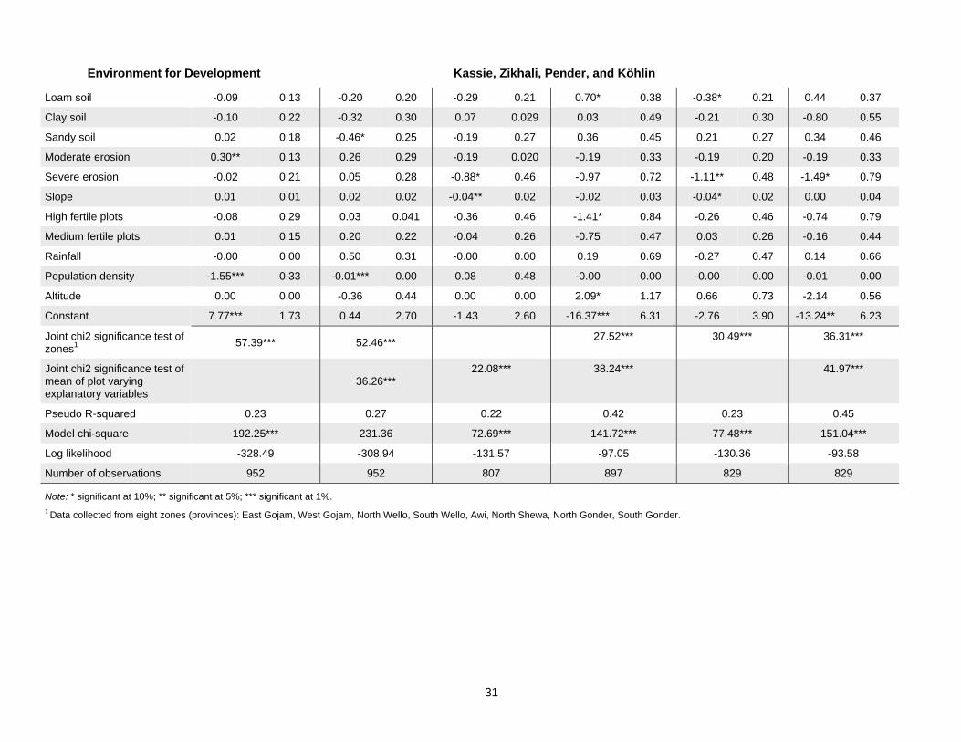
Loam soil -0.09 0.13 -0.20 0.20 -0.29 0.21 0.70* 0.38 -0.38* 0.21 0.44 0.37
Clay soil -0.10 0.22 -0.32 0.30 0.07 0.029 0.03 0.49 -0.21 0.30 -0.80 0.55
Sandy soil 0.02 0.18 -0.46* 0.25 -0.19 0.27 0.36 0.45 0.21 0.27 0.34 0.46
Moderate erosion 0.30** 0.13 0.26 0.29 -0.19 0.020 -0.19 0.33 -0.19 0.20 -0.19 0.33
Severe erosion -0.02 0.21 0.05 0.28 -0.88* 0.46 -0.97 0.72 -1.11** 0.48 -1.49* 0.79
Slope 0.01 0.01 0.02 0.02 -0.04** 0.02 -0.02 0.03 -0.04* 0.02 0.00 0.04
High fertile plots -0.08 0.29 0.03 0.041 -0.36 0.46 -1.41* 0.84 -0.26 0.46 -0.74 0.79
Medium fertile plots 0.01 0.15 0.20 0.22 -0.04 0.26 -0.75 0.47 0.03 0.26 -0.16 0.44
Rainfall -0.00 0.00 0.50 0.31 -0.00 0.00 0.19 0.69 -0.27 0.47 0.14 0.66
Population density -1.55*** 0.33 -0.01*** 0.00 0.08 0.48 -0.00 0.00 -0.00 0.00 -0.01 0.00
Altitude 0.00 0.00 -0.36 0.44 0.00 0.00 2.09* 1.17 0.66 0.73 -2.14 0.56
Constant 7.77*** 1.73 0.44 2.70 -1.43 2.60 -16.37*** 6.31 -2.76 3.90 -13.24** 6.23
Joint chi2 significance test of zones1 57.39*** 52.46*** 27.52*** 30.49*** 36.31***
Joint chi2 significance test of mean of plot varying explanatory variables
36.26*** 22.08*** 38.24*** 41.97***
Pseudo R-squared 0.23 0.27 0.22 0.42 0.23 0.45
Model chi-square 192.25*** 231.36 72.69*** 141.72*** 77.48*** 151.04***
Log likelihood -328.49 -308.94 -131.57 -97.05 -130.36 -93.58
Number of observations 952 952 807 897 829 829
Note: * significant at 10%; ** significant at 5%; *** significant at 1%. 1 Data collected from eight zones (provinces): East Gojam, West Gojam, North Wello, South Wello, Awi, North Shewa, North Gonder, South Gonder.
Environment for Development Kassie, Zikhali, Pender, and Köhlin
32
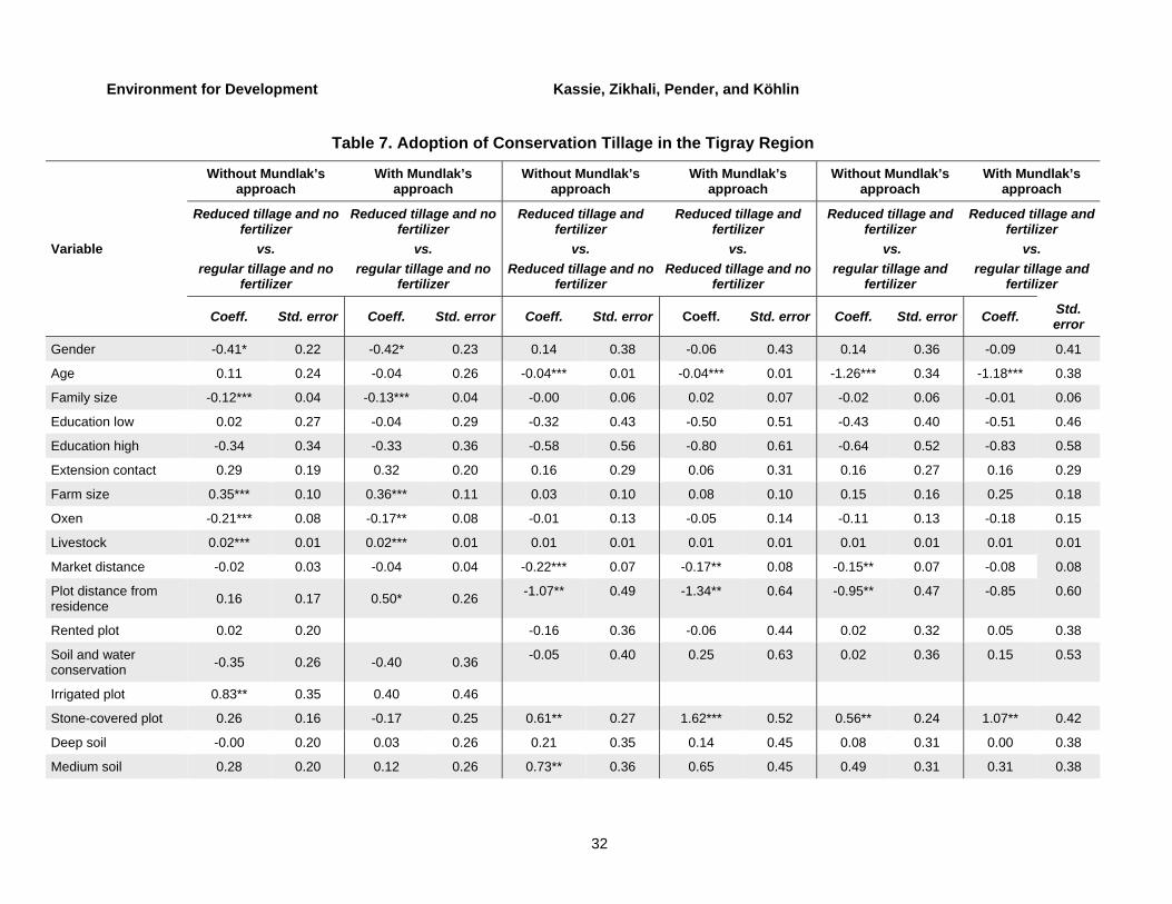
Table 7. Adoption of Conservation Tillage in the Tigray Region
Variable
Without Mundlak’s approach
With Mundlak’s approach
Without Mundlak’s approach
With Mundlak’s approach
Without Mundlak’s approach
With Mundlak’s approach
Reduced tillage and no fertilizer
vs. regular tillage and no
fertilizer
Reduced tillage and no fertilizer
vs. regular tillage and no
fertilizer
Reduced tillage and fertilizer
vs. Reduced tillage and no
fertilizer
Reduced tillage and fertilizer
vs. Reduced tillage and no
fertilizer
Reduced tillage and fertilizer
vs. regular tillage and
fertilizer
Reduced tillage and fertilizer
vs. regular tillage and
fertilizer
Coeff. Std. error Coeff. Std. error Coeff. Std. error Coeff. Std. error Coeff. Std. error Coeff. Std. error
Gender -0.41* 0.22 -0.42* 0.23 0.14 0.38 -0.06 0.43 0.14 0.36 -0.09 0.41
Age 0.11 0.24 -0.04 0.26 -0.04*** 0.01 -0.04*** 0.01 -1.26*** 0.34 -1.18*** 0.38
Family size -0.12*** 0.04 -0.13*** 0.04 -0.00 0.06 0.02 0.07 -0.02 0.06 -0.01 0.06
Education low 0.02 0.27 -0.04 0.29 -0.32 0.43 -0.50 0.51 -0.43 0.40 -0.51 0.46
Education high -0.34 0.34 -0.33 0.36 -0.58 0.56 -0.80 0.61 -0.64 0.52 -0.83 0.58
Extension contact 0.29 0.19 0.32 0.20 0.16 0.29 0.06 0.31 0.16 0.27 0.16 0.29
Farm size 0.35*** 0.10 0.36*** 0.11 0.03 0.10 0.08 0.10 0.15 0.16 0.25 0.18
Oxen -0.21*** 0.08 -0.17** 0.08 -0.01 0.13 -0.05 0.14 -0.11 0.13 -0.18 0.15
Livestock 0.02*** 0.01 0.02*** 0.01 0.01 0.01 0.01 0.01 0.01 0.01 0.01 0.01
Market distance -0.02 0.03 -0.04 0.04 -0.22*** 0.07 -0.17** 0.08 -0.15** 0.07 -0.08 0.08
Plot distance from residence 0.16 0.17 0.50* 0.26 -1.07** 0.49 -1.34** 0.64 -0.95** 0.47 -0.85 0.60
Rented plot 0.02 0.20 -0.16 0.36 -0.06 0.44 0.02 0.32 0.05 0.38
Soil and water conservation -0.35 0.26 -0.40 0.36 -0.05 0.40 0.25 0.63 0.02 0.36 0.15 0.53
Irrigated plot 0.83** 0.35 0.40 0.46
Stone-covered plot 0.26 0.16 -0.17 0.25 0.61** 0.27 1.62*** 0.52 0.56** 0.24 1.07** 0.42
Deep soil -0.00 0.20 0.03 0.26 0.21 0.35 0.14 0.45 0.08 0.31 0.00 0.38
Medium soil 0.28 0.20 0.12 0.26 0.73** 0.36 0.65 0.45 0.49 0.31 0.31 0.38
Environment for Development Kassie, Zikhali, Pender, and Köhlin
33
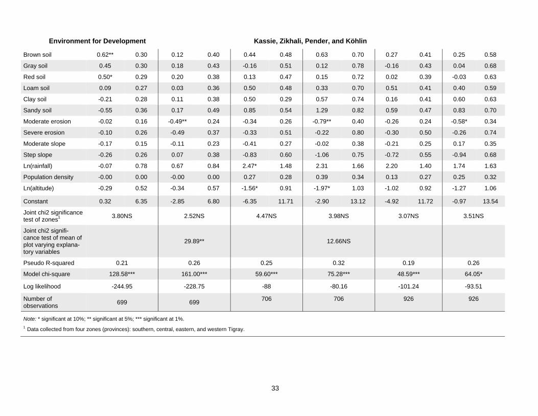
Brown soil 0.62** 0.30 0.12 0.40 0.44 0.48 0.63 0.70 0.27 0.41 0.25 0.58
Gray soil 0.45 0.30 0.18 0.43 -0.16 0.51 0.12 0.78 -0.16 0.43 0.04 0.68
Red soil 0.50* 0.29 0.20 0.38 0.13 0.47 0.15 0.72 0.02 0.39 -0.03 0.63
Loam soil 0.09 0.27 0.03 0.36 0.50 0.48 0.33 0.70 0.51 0.41 0.40 0.59
Clay soil -0.21 0.28 0.11 0.38 0.50 0.29 0.57 0.74 0.16 0.41 0.60 0.63
Sandy soil -0.55 0.36 0.17 0.49 0.85 0.54 1.29 0.82 0.59 0.47 0.83 0.70
Moderate erosion -0.02 0.16 -0.49** 0.24 -0.34 0.26 -0.79** 0.40 -0.26 0.24 -0.58* 0.34
Severe erosion -0.10 0.26 -0.49 0.37 -0.33 0.51 -0.22 0.80 -0.30 0.50 -0.26 0.74
Moderate slope -0.17 0.15 -0.11 0.23 -0.41 0.27 -0.02 0.38 -0.21 0.25 0.17 0.35
Step slope -0.26 0.26 0.07 0.38 -0.83 0.60 -1.06 0.75 -0.72 0.55 -0.94 0.68
Ln(rainfall) -0.07 0.78 0.67 0.84 2.47* 1.48 2.31 1.66 2.20 1.40 1.74 1.63
Population density -0.00 0.00 -0.00 0.00 0.27 0.28 0.39 0.34 0.13 0.27 0.25 0.32
Ln(altitude) -0.29 0.52 -0.34 0.57 -1.56* 0.91 -1.97* 1.03 -1.02 0.92 -1.27 1.06
Constant 0.32 6.35 -2.85 6.80 -6.35 11.71 -2.90 13.12 -4.92 11.72 -0.97 13.54
Joint chi2 significance test of zones1 3.80NS 2.52NS 4.47NS 3.98NS 3.07NS 3.51NS
Joint chi2 signifi-cance test of mean of plot varying explana-tory variables
29.89** 12.66NS
Pseudo R-squared 0.21 0.26 0.25 0.32 0.19 0.26
Model chi-square 128.58*** 161.00*** 59.60*** 75.28*** 48.59*** 64.05*
Log likelihood -244.95 -228.75 -88 -80.16 -101.24 -93.51
Number of observations 699 699 706 706 926 926
Note: * significant at 10%; ** significant at 5%; *** significant at 1%. 1 Data collected from four zones (provinces): southern, central, eastern, and western Tigray.

Environment for Development Kassie, Zikhali, Pender, and Köhlin
34
Table 8. Productivity Impacts from Semi-Parametric Regression Analysis
Model 1 Model 2 Model 3 Model 4
Fertilizer and regular tillage
vs. no fertilizer and regular tillage
Reduced tillage and no fertilizer
vs. regular tillage and
no fertilizer
Reduced tillage and fertilizer
vs. Reduced tillage and no fertilizer
Reduced tillage and fertilizer
vs. regular tillage and
fertilizer
With Mundlak’s approach
Amhara Region
ATT 1180.841*** 39.902 402.743 583.144
Standard error 357.036 185.279 392.915 363.917
Number of observations
Treated 370 156 43 43
Control 197 105 38 34
Tigray Region
ATT 88.098 738.818*** 712.198* 902.697*
Standard error 188.750 321.111 419.603 478.863
Number of observations
Treated 340 113 28 28
Control 209 78 28 26
Without Mundlak’s approach
Amhara region
ATT 1020.141** 43.224 159.898 -43.491
Standard error 431.564 199.887 402.661 383.008
Number of observations
Treated 370 156 43 43
Control 174 105 28 31
Tigray region
ATT 70.170 695.336*** 672.373 * 624.388
Standard error 153.171 290.621 357.772 518.357
Number of observations
Treated 340 113 28 28
Control 197 71 25 26
Note: * significant at 10%; ** significant at 5%; *** significant at 1%.
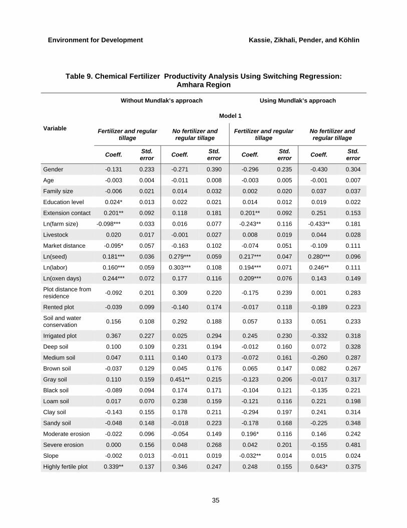
Environment for Development Kassie, Zikhali, Pender, and Köhlin
35
Table 9. Chemical Fertilizer Productivity Analysis Using Switching Regression: Amhara Region
Variable
Without Mundlak’s approach Using Mundlak’s approach
Model 1
Fertilizer and regular tillage
No fertilizer and regular tillage
Fertilizer and regular tillage
No fertilizer and regular tillage
Coeff. Std. error Coeff. Std.
error Coeff. Std. error Coeff. Std.
error
Gender -0.131 0.233 -0.271 0.390 -0.296 0.235 -0.430 0.304
Age -0.003 0.004 -0.011 0.008 -0.003 0.005 -0.001 0.007
Family size -0.006 0.021 0.014 0.032 0.002 0.020 0.037 0.037
Education level 0.024* 0.013 0.022 0.021 0.014 0.012 0.019 0.022
Extension contact 0.201** 0.092 0.118 0.181 0.201** 0.092 0.251 0.153
Ln(farm size) -0.098*** 0.033 0.016 0.077 -0.243** 0.116 -0.433** 0.181
Livestock 0.020 0.017 -0.001 0.027 0.008 0.019 0.044 0.028
Market distance -0.095* 0.057 -0.163 0.102 -0.074 0.051 -0.109 0.111
Ln(seed) 0.181*** 0.036 0.279*** 0.059 0.217*** 0.047 0.280*** 0.096
Ln(labor) 0.160*** 0.059 0.303*** 0.108 0.194*** 0.071 0.246** 0.111
Ln(oxen days) 0.244*** 0.072 0.177 0.116 0.209*** 0.076 0.143 0.149
Plot distance from residence -0.092 0.201 0.309 0.220 -0.175 0.239 0.001 0.283
Rented plot -0.039 0.099 -0.140 0.174 -0.017 0.118 -0.189 0.223
Soil and water conservation 0.156 0.108 0.292 0.188 0.057 0.133 0.051 0.233
Irrigated plot 0.367 0.227 0.025 0.294 0.245 0.230 -0.332 0.318
Deep soil 0.100 0.109 0.231 0.194 -0.012 0.160 0.072 0.328
Medium soil 0.047 0.111 0.140 0.173 -0.072 0.161 -0.260 0.287
Brown soil -0.037 0.129 0.045 0.176 0.065 0.147 0.082 0.267
Gray soil 0.110 0.159 0.451** 0.215 -0.123 0.206 -0.017 0.317
Black soil -0.089 0.094 0.174 0.171 -0.104 0.121 -0.135 0.221
Loam soil 0.017 0.070 0.238 0.159 -0.121 0.116 0.221 0.198
Clay soil -0.143 0.155 0.178 0.211 -0.294 0.197 0.241 0.314
Sandy soil -0.048 0.148 -0.018 0.223 -0.178 0.168 -0.225 0.348
Moderate erosion -0.022 0.096 -0.054 0.149 0.196* 0.116 0.146 0.242
Severe erosion 0.000 0.156 0.048 0.268 0.042 0.201 -0.155 0.481
Slope -0.002 0.013 -0.011 0.019 -0.032** 0.014 0.015 0.024
Highly fertile plot 0.339** 0.137 0.346 0.247 0.248 0.155 0.643* 0.375
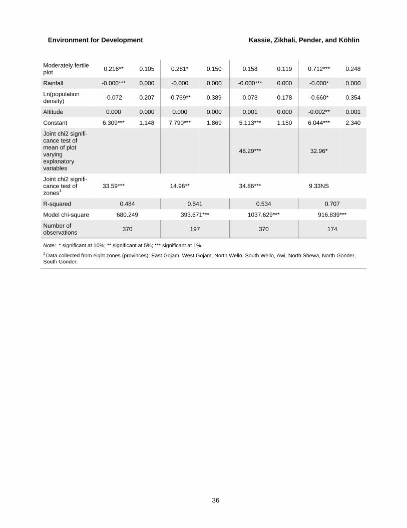
Environment for Development Kassie, Zikhali, Pender, and Köhlin
36
Moderately fertile plot 0.216** 0.105 0.281* 0.150 0.158 0.119 0.712*** 0.248
Rainfall -0.000*** 0.000 -0.000 0.000 -0.000*** 0.000 -0.000* 0.000
Ln(population density) -0.072 0.207 -0.769** 0.389 0.073 0.178 -0.660* 0.354
Altitude 0.000 0.000 0.000 0.000 0.001 0.000 -0.002** 0.001
Constant 6.309*** 1.148 7.790*** 1.869 5.113*** 1.150 6.044*** 2.340
Joint chi2 signifi-cance test of mean of plot varying explanatory variables
48.29*** 32.96*
Joint chi2 signifi-cance test of zones1
33.59*** 14.96** 34.86*** 9.33NS
R-squared 0.484 0.541 0.534 0.707
Model chi-square 680.249 393.671*** 1037.629*** 916.839***
Number of observations 370 197 370 174
Note: * significant at 10%; ** significant at 5%; *** significant at 1%. 1 Data collected from eight zones (provinces): East Gojam, West Gojam, North Wello, South Wello, Awi, North Shewa, North Gonder, South Gonder.
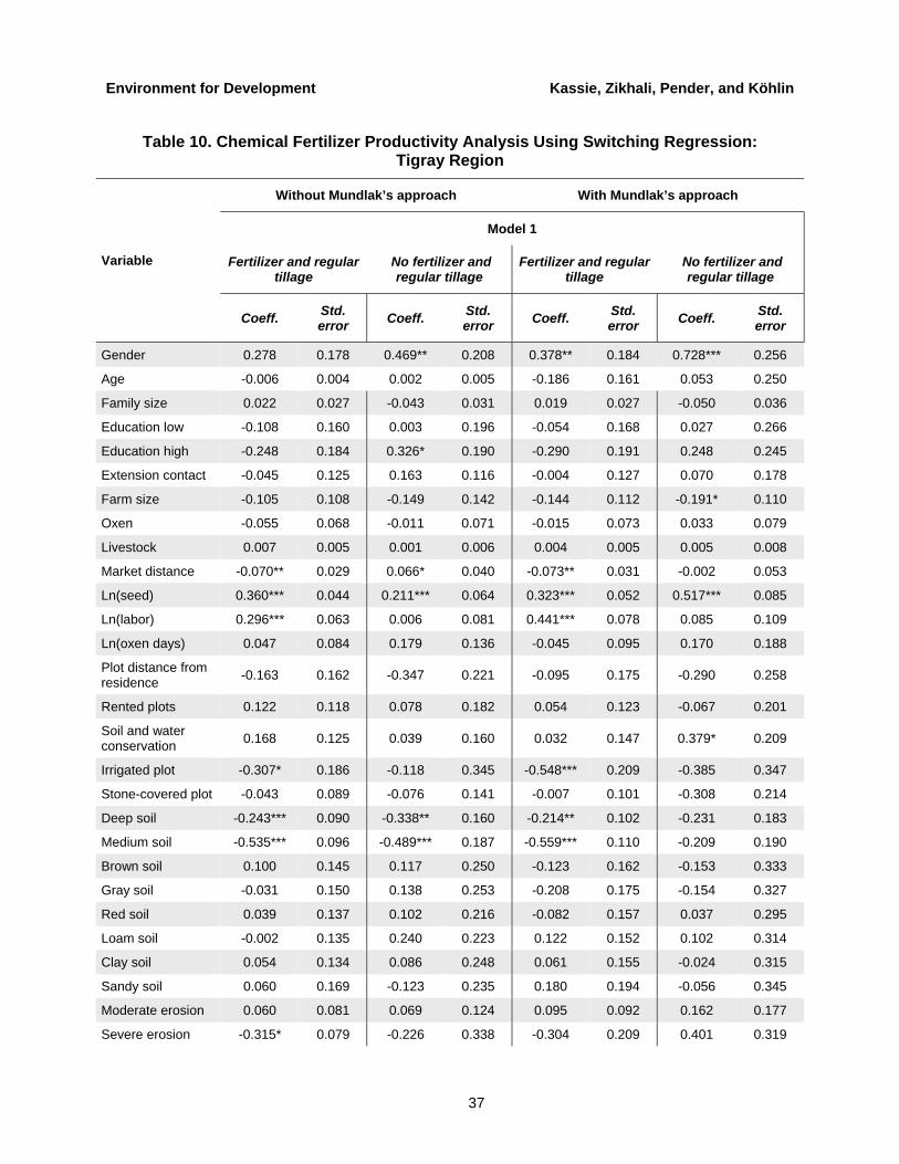
Environment for Development Kassie, Zikhali, Pender, and Köhlin
37
Table 10. Chemical Fertilizer Productivity Analysis Using Switching Regression: Tigray Region
Variable
Without Mundlak’s approach With Mundlak’s approach
Model 1
Fertilizer and regular tillage
No fertilizer and regular tillage
Fertilizer and regular tillage
No fertilizer and regular tillage
Coeff. Std. error Coeff. Std.
error Coeff. Std. error Coeff. Std.
error
Gender 0.278 0.178 0.469** 0.208 0.378** 0.184 0.728*** 0.256
Age -0.006 0.004 0.002 0.005 -0.186 0.161 0.053 0.250
Family size 0.022 0.027 -0.043 0.031 0.019 0.027 -0.050 0.036
Education low -0.108 0.160 0.003 0.196 -0.054 0.168 0.027 0.266
Education high -0.248 0.184 0.326* 0.190 -0.290 0.191 0.248 0.245
Extension contact -0.045 0.125 0.163 0.116 -0.004 0.127 0.070 0.178
Farm size -0.105 0.108 -0.149 0.142 -0.144 0.112 -0.191* 0.110
Oxen -0.055 0.068 -0.011 0.071 -0.015 0.073 0.033 0.079
Livestock 0.007 0.005 0.001 0.006 0.004 0.005 0.005 0.008
Market distance -0.070** 0.029 0.066* 0.040 -0.073** 0.031 -0.002 0.053
Ln(seed) 0.360*** 0.044 0.211*** 0.064 0.323*** 0.052 0.517*** 0.085
Ln(labor) 0.296*** 0.063 0.006 0.081 0.441*** 0.078 0.085 0.109
Ln(oxen days) 0.047 0.084 0.179 0.136 -0.045 0.095 0.170 0.188
Plot distance from residence -0.163 0.162 -0.347 0.221 -0.095 0.175 -0.290 0.258
Rented plots 0.122 0.118 0.078 0.182 0.054 0.123 -0.067 0.201
Soil and water conservation 0.168 0.125 0.039 0.160 0.032 0.147 0.379* 0.209
Irrigated plot -0.307* 0.186 -0.118 0.345 -0.548*** 0.209 -0.385 0.347
Stone-covered plot -0.043 0.089 -0.076 0.141 -0.007 0.101 -0.308 0.214
Deep soil -0.243*** 0.090 -0.338** 0.160 -0.214** 0.102 -0.231 0.183
Medium soil -0.535*** 0.096 -0.489*** 0.187 -0.559*** 0.110 -0.209 0.190
Brown soil 0.100 0.145 0.117 0.250 -0.123 0.162 -0.153 0.333
Gray soil -0.031 0.150 0.138 0.253 -0.208 0.175 -0.154 0.327
Red soil 0.039 0.137 0.102 0.216 -0.082 0.157 0.037 0.295
Loam soil -0.002 0.135 0.240 0.223 0.122 0.152 0.102 0.314
Clay soil 0.054 0.134 0.086 0.248 0.061 0.155 -0.024 0.315
Sandy soil 0.060 0.169 -0.123 0.235 0.180 0.194 -0.056 0.345
Moderate erosion 0.060 0.081 0.069 0.124 0.095 0.092 0.162 0.177
Severe erosion -0.315* 0.079 -0.226 0.338 -0.304 0.209 0.401 0.319
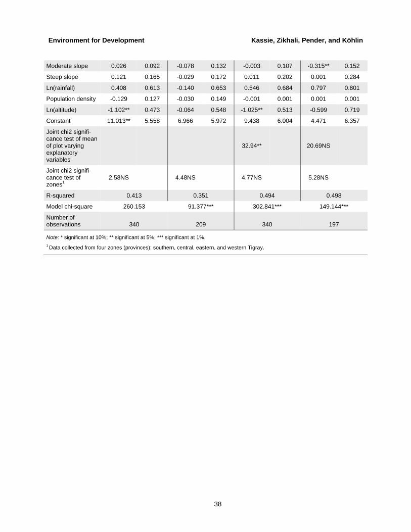
Environment for Development Kassie, Zikhali, Pender, and Köhlin
38
Moderate slope 0.026 0.092 -0.078 0.132 -0.003 0.107 -0.315** 0.152
Steep slope 0.121 0.165 -0.029 0.172 0.011 0.202 0.001 0.284
Ln(rainfall) 0.408 0.613 -0.140 0.653 0.546 0.684 0.797 0.801
Population density -0.129 0.127 -0.030 0.149 -0.001 0.001 0.001 0.001
Ln(altitude) -1.102** 0.473 -0.064 0.548 -1.025** 0.513 -0.599 0.719
Constant 11.013** 5.558 6.966 5.972 9.438 6.004 4.471 6.357
Joint chi2 signifi-cance test of mean of plot varying explanatory variables
32.94** 20.69NS
Joint chi2 signifi-cance test of zones1
2.58NS 4.48NS 4.77NS 5.28NS
R-squared 0.413 0.351 0.494 0.498
Model chi-square 260.153 91.377*** 302.841*** 149.144***
Number of observations 340 209 340 197
Note: * significant at 10%; ** significant at 5%; *** significant at 1%. 1 Data collected from four zones (provinces): southern, central, eastern, and western Tigray.
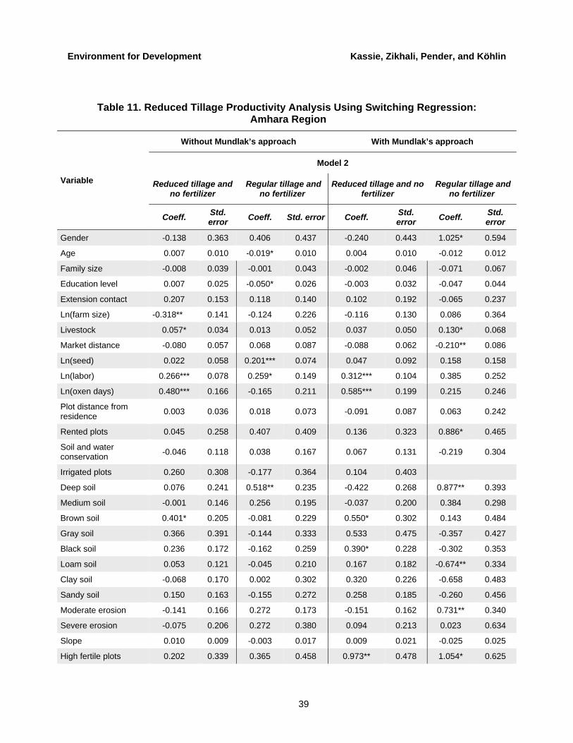
Environment for Development Kassie, Zikhali, Pender, and Köhlin
39
Table 11. Reduced Tillage Productivity Analysis Using Switching Regression: Amhara Region
Variable
Without Mundlak’s approach With Mundlak’s approach
Model 2
Reduced tillage and no fertilizer
Regular tillage and no fertilizer
Reduced tillage and no fertilizer
Regular tillage and no fertilizer
Coeff. Std. error Coeff. Std. error Coeff. Std.
error Coeff. Std. error
Gender -0.138 0.363 0.406 0.437 -0.240 0.443 1.025* 0.594
Age 0.007 0.010 -0.019* 0.010 0.004 0.010 -0.012 0.012
Family size -0.008 0.039 -0.001 0.043 -0.002 0.046 -0.071 0.067
Education level 0.007 0.025 -0.050* 0.026 -0.003 0.032 -0.047 0.044
Extension contact 0.207 0.153 0.118 0.140 0.102 0.192 -0.065 0.237
Ln(farm size) -0.318** 0.141 -0.124 0.226 -0.116 0.130 0.086 0.364
Livestock 0.057* 0.034 0.013 0.052 0.037 0.050 0.130* 0.068
Market distance -0.080 0.057 0.068 0.087 -0.088 0.062 -0.210** 0.086
Ln(seed) 0.022 0.058 0.201*** 0.074 0.047 0.092 0.158 0.158
Ln(labor) 0.266*** 0.078 0.259* 0.149 0.312*** 0.104 0.385 0.252
Ln(oxen days) 0.480*** 0.166 -0.165 0.211 0.585*** 0.199 0.215 0.246
Plot distance from residence 0.003 0.036 0.018 0.073 -0.091 0.087 0.063 0.242
Rented plots 0.045 0.258 0.407 0.409 0.136 0.323 0.886* 0.465
Soil and water conservation -0.046 0.118 0.038 0.167 0.067 0.131 -0.219 0.304
Irrigated plots 0.260 0.308 -0.177 0.364 0.104 0.403
Deep soil 0.076 0.241 0.518** 0.235 -0.422 0.268 0.877** 0.393
Medium soil -0.001 0.146 0.256 0.195 -0.037 0.200 0.384 0.298
Brown soil 0.401* 0.205 -0.081 0.229 0.550* 0.302 0.143 0.484
Gray soil 0.366 0.391 -0.144 0.333 0.533 0.475 -0.357 0.427
Black soil 0.236 0.172 -0.162 0.259 0.390* 0.228 -0.302 0.353
Loam soil 0.053 0.121 -0.045 0.210 0.167 0.182 -0.674** 0.334
Clay soil -0.068 0.170 0.002 0.302 0.320 0.226 -0.658 0.483
Sandy soil 0.150 0.163 -0.155 0.272 0.258 0.185 -0.260 0.456
Moderate erosion -0.141 0.166 0.272 0.173 -0.151 0.162 0.731** 0.340
Severe erosion -0.075 0.206 0.272 0.380 0.094 0.213 0.023 0.634
Slope 0.010 0.009 -0.003 0.017 0.009 0.021 -0.025 0.025
High fertile plots 0.202 0.339 0.365 0.458 0.973** 0.478 1.054* 0.625

Environment for Development Kassie, Zikhali, Pender, and Köhlin
40
Medium fertile plots 0.311** 0.135 0.347 0.229 0.452** 0.184 0.584 0.448
Rainfall 0.000 0.000 0.000 0.000 -0.120 0.395 0.195 0.685
Ln(population density) 0.120 0.454 0.123 0.491 0.002 0.003 0.159 0.769
Altitude -0.000 0.000 -0.000 0.000 0.474 0.407 -0.480 0.805
Constant 2.776 2.267 4.791** 2.291 2.038 3.492 6.180 4.014
Joint chi2 significance test of mean of plot varying explanatory variables
34.55** 2.84***
Joint chi2 significance test of zones1 20.36*** 1.44NS 10.57 2.11*
R-squared 0.520 0.295 0.586 0.690
Model chi-square 376.609*** 2.14*** 971.441*** 15.22***
Number of observations 156 105 156 105
Note: * significant at 10%; ** significant at 5%; *** significant at 1%. 1 Data collected from eight zones (provinces): East Gojam, West Gojam, North Wello, South Wello, Awi, North Shewa, North Gonder, South Gonder.
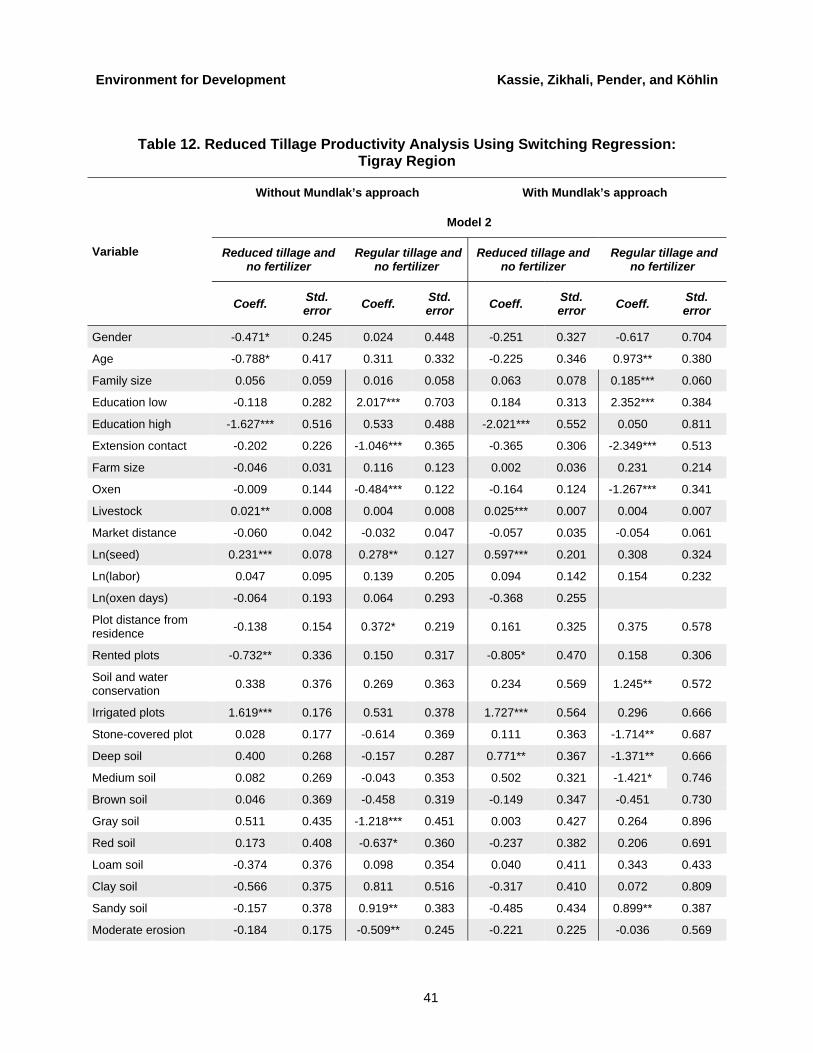
Environment for Development Kassie, Zikhali, Pender, and Köhlin
41
Table 12. Reduced Tillage Productivity Analysis Using Switching Regression: Tigray Region
Variable
Without Mundlak’s approach With Mundlak’s approach
Model 2
Reduced tillage and no fertilizer
Regular tillage and no fertilizer
Reduced tillage and no fertilizer
Regular tillage and no fertilizer
Coeff. Std. error Coeff. Std.
error Coeff. Std. error Coeff. Std.
error
Gender -0.471* 0.245 0.024 0.448 -0.251 0.327 -0.617 0.704
Age -0.788* 0.417 0.311 0.332 -0.225 0.346 0.973** 0.380
Family size 0.056 0.059 0.016 0.058 0.063 0.078 0.185*** 0.060
Education low -0.118 0.282 2.017*** 0.703 0.184 0.313 2.352*** 0.384
Education high -1.627*** 0.516 0.533 0.488 -2.021*** 0.552 0.050 0.811
Extension contact -0.202 0.226 -1.046*** 0.365 -0.365 0.306 -2.349*** 0.513
Farm size -0.046 0.031 0.116 0.123 0.002 0.036 0.231 0.214
Oxen -0.009 0.144 -0.484*** 0.122 -0.164 0.124 -1.267*** 0.341
Livestock 0.021** 0.008 0.004 0.008 0.025*** 0.007 0.004 0.007
Market distance -0.060 0.042 -0.032 0.047 -0.057 0.035 -0.054 0.061
Ln(seed) 0.231*** 0.078 0.278** 0.127 0.597*** 0.201 0.308 0.324
Ln(labor) 0.047 0.095 0.139 0.205 0.094 0.142 0.154 0.232
Ln(oxen days) -0.064 0.193 0.064 0.293 -0.368 0.255
Plot distance from residence -0.138 0.154 0.372* 0.219 0.161 0.325 0.375 0.578
Rented plots -0.732** 0.336 0.150 0.317 -0.805* 0.470 0.158 0.306
Soil and water conservation 0.338 0.376 0.269 0.363 0.234 0.569 1.245** 0.572
Irrigated plots 1.619*** 0.176 0.531 0.378 1.727*** 0.564 0.296 0.666
Stone-covered plot 0.028 0.177 -0.614 0.369 0.111 0.363 -1.714** 0.687
Deep soil 0.400 0.268 -0.157 0.287 0.771** 0.367 -1.371** 0.666
Medium soil 0.082 0.269 -0.043 0.353 0.502 0.321 -1.421* 0.746
Brown soil 0.046 0.369 -0.458 0.319 -0.149 0.347 -0.451 0.730
Gray soil 0.511 0.435 -1.218*** 0.451 0.003 0.427 0.264 0.896
Red soil 0.173 0.408 -0.637* 0.360 -0.237 0.382 0.206 0.691
Loam soil -0.374 0.376 0.098 0.354 0.040 0.411 0.343 0.433
Clay soil -0.566 0.375 0.811 0.516 -0.317 0.410 0.072 0.809
Sandy soil -0.157 0.378 0.919** 0.383 -0.485 0.434 0.899** 0.387
Moderate erosion -0.184 0.175 -0.509** 0.245 -0.221 0.225 -0.036 0.569
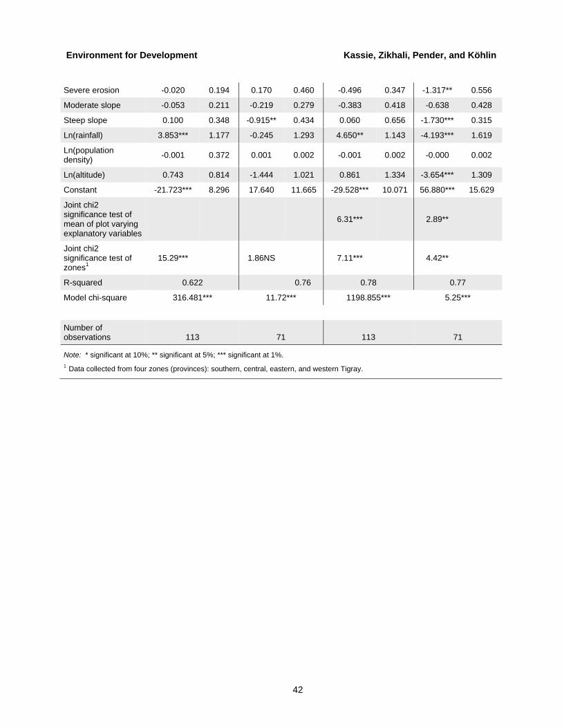
Environment for Development Kassie, Zikhali, Pender, and Köhlin
42
Severe erosion -0.020 0.194 0.170 0.460 -0.496 0.347 -1.317** 0.556
Moderate slope -0.053 0.211 -0.219 0.279 -0.383 0.418 -0.638 0.428
Steep slope 0.100 0.348 -0.915** 0.434 0.060 0.656 -1.730*** 0.315
Ln(rainfall) 3.853*** 1.177 -0.245 1.293 4.650** 1.143 -4.193*** 1.619
Ln(population density) -0.001 0.372 0.001 0.002 -0.001 0.002 -0.000 0.002
Ln(altitude) 0.743 0.814 -1.444 1.021 0.861 1.334 -3.654*** 1.309
Constant -21.723*** 8.296 17.640 11.665 -29.528*** 10.071 56.880*** 15.629
Joint chi2 significance test of mean of plot varying explanatory variables
6.31*** 2.89**
Joint chi2 significance test of zones1
15.29*** 1.86NS 7.11*** 4.42**
R-squared 0.622 0.76 0.78 0.77
Model chi-square 316.481*** 11.72*** 1198.855*** 5.25***
Number of observations 113 71 113 71
Note: * significant at 10%; ** significant at 5%; *** significant at 1%. 1 Data collected from four zones (provinces): southern, central, eastern, and western Tigray.
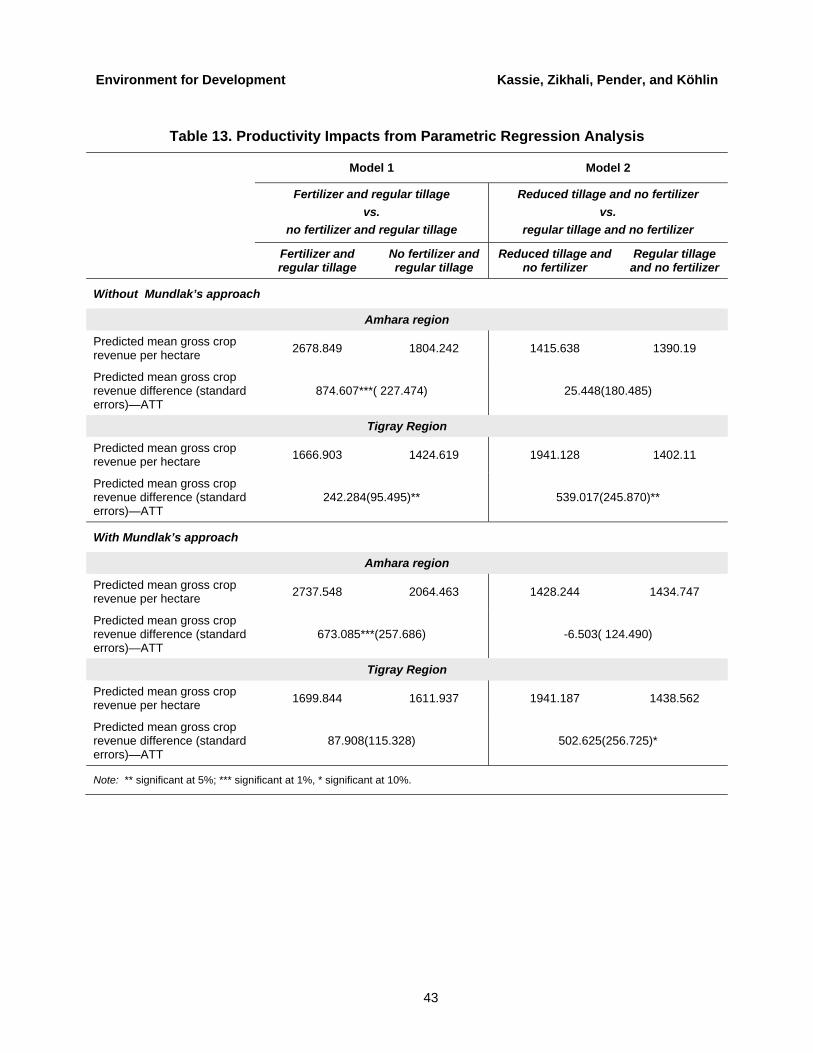
Environment for Development Kassie, Zikhali, Pender, and Köhlin
43
Table 13. Productivity Impacts from Parametric Regression Analysis
Model 1 Model 2
Fertilizer and regular tillage vs.
no fertilizer and regular tillage
Reduced tillage and no fertilizer vs.
regular tillage and no fertilizer
Fertilizer and regular tillage
No fertilizer and regular tillage
Reduced tillage and no fertilizer
Regular tillage and no fertilizer
Without Mundlak’s approach
Amhara region
Predicted mean gross crop revenue per hectare 2678.849 1804.242 1415.638 1390.19
Predicted mean gross crop revenue difference (standard errors)—ATT
874.607***( 227.474) 25.448(180.485)
Tigray Region
Predicted mean gross crop revenue per hectare 1666.903 1424.619 1941.128 1402.11
Predicted mean gross crop revenue difference (standard errors)—ATT
242.284(95.495)** 539.017(245.870)**
With Mundlak’s approach
Amhara region
Predicted mean gross crop revenue per hectare 2737.548 2064.463 1428.244 1434.747
Predicted mean gross crop revenue difference (standard errors)—ATT
673.085***(257.686) -6.503( 124.490)
Tigray Region
Predicted mean gross crop revenue per hectare 1699.844 1611.937 1941.187 1438.562
Predicted mean gross crop revenue difference (standard errors)—ATT
87.908(115.328) 502.625(256.725)*
Note: ** significant at 5%; *** significant at 1%, * significant at 10%.