Survey Bmis 2011

8/3/2019 Survey Bmis 2011

http://slidepdf.com/reader/full/survey-bmis-2011 1/73

Short Survey of Brain Machine Interfaces

Jose C. Principe, Ph.D.Distinguished Professor ECE, BME

Computational NeuroEngineering LaboratoryElectrical and Computer Engineering Department

University of Floridawww.cnel.ufl.edu

[email protected]

http://www.cnel.ufl.edu/

http://www.cnel.ufl.edu/



Acknowledgments

Dr. Justin Sanchez, University of Florida

Dr. Phil Kim, Brown University

My students: Yiwen WangAntonio PaivaIl ParkAysegul Gunduz

NSF (DDDAS, CRCNS), NIH NIBIB, DARPA



Outline

Brain Machine InterfaceDefinitionsTypes

Hardware challengesBMI Models using rate codesBMI Models using spike trains



Why is a New Neurotechnology Emerging?

Synergistic advances inNeuroscience

Understanding the brain as information processingsystem, localization, coding

Physical InterfacesTiny size, stable materials, effective at sensing andstimulating

Device miniaturizationLow power electronics, fast computers, algorithms



Brain Machine Interfaces (BMI)

A man made device that either substitutes asensory input to the brain, repairs functionalcommunication between brain regions ortranslates intention of movement.



Deep Brain Stimulation (DBS)

Donoghue, 2005

Parkinson's disease

Medtronics



Vagal Nerve Stimulation

EpilepsyMood disorders

Cyberonics



Cochlear Implants

(http://www.cochlear.com)

Electronics(12-22 channels)

battery

microphone

Headpiece(antenna)

Internal receiverstimulator

wires

Electrodes(12-22)

AuditoryNerve



Visual prosthesis

Prof. J. Lobo Antunes was involved in this project

http://www.artificialvision.com/vision/asaio1.html



Cognitive/Memory Prosthesis

Berger et al, 2008

damage



Neuromotor ProsthesisFrom Thought to Action

Many neuropathies leave cognition intact but disrupt thecontrol of the motor system

Spinal cord injury

ALSCerebral palsyStrokeLock-in syndromeMuscular dystrophy/atrophyLimb loss

Goal is to bypass the motor system and create a directpath between the cortex and an external device.



Proof of Concept…and media fanfare!

What are the underlying principles behind neural control of devices?



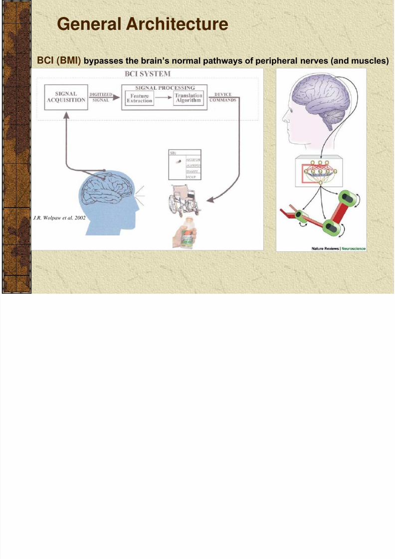
J.R. Wolpaw et al. 2002

BCI (BMI) bypasses the brain’s normal pathways of peripheral nerves (and muscles)

General Architecture



INTENT

PERCEPT

ACTION

STIMULUS

Decoding

Coding

BRAIN MACHINE

Neural Interface Physical Interface

The Fundamental Concept

Stimulus Neural Response

Coding Given To be inferred

Decoding To be inferred Given

Need to understand how brain processes information .



Levels of Abstraction for Neurotechnology

Brain is an extremelycomplex system

10 12 neurons

1015

synapsesSpecificinterconnectivity



Tapping into the Nervous System

The choice and availability of brain signals andrecording methods can greatly influence the ultimateperformance of the BMI.

The level of BMI performance may be attributed toselection of electrode technology, choice of model , andmethods for extracting rate, frequency , or timing codes.



http://ida.first.fhg.de/projects/bci/bbci_official/

Coarse(mm)



Choice of Scale for Neuroprosthetics

Bandwidth(approximate) Localization

ScalpElectrodes

0 ~ 80 Hz VolumeConductionCortical Surface

Electro-corticogram(ECoG)

0 ~ 500Hz Cortical Surface

Implanted

Electrodes

0 ~ 7kHz Single Neuron



Spatial Resolution of Recordings

Moran


http://slidepdf.com/reader/full/survey-bmis-2011 22/735/5/2012 22

Examples of Multiscale Signals

Scalp EEGPenfield

Spikes andLFPs

In vivo extracellular



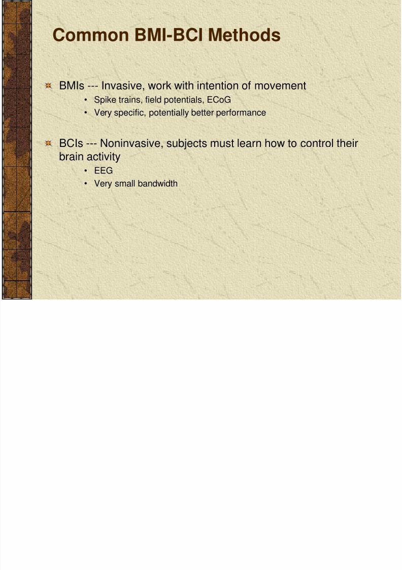
Common BMI-BCI Methods

BMIs --- Invasive, work with intention of movement• Spike trains, field potentials, ECoG• Very specific, potentially better performance

BCIs --- Noninvasive, subjects must learn how to control theirbrain activity

• EEG• Very small bandwidth



Brain Computer Interfaces (BCI) EEG

Sensory Motor Rhythm

Wasdworth Center, NY



How to put it together?

NeoCortical Brain Areas Related to Movement

Posterior Parietal (PP) – Visual to motortransformation

Premotor (PM) and DorsalPremotor (PMD) -

Planning and guidance

(visual inputs)

Primary Motor (M1) – Initiates muscle contraction



Electrophysiology:Electrode Arrays

50 μm polyimide insulatedtungsten250 μm separationWire impedance of 500K – 1.5M Ω



two polyimide cables

•Flexible polyimide cableintegrated with rigid metalelectrodes

Design StrategyMetal electrodes(array of 16)

Glass (Pyrex) wafer

Cured Polyimide

Sputter nickel, pattern via lift-off

Coat with polyimide,Etch polyimide from contact pads &probe tip, Insulate free probe tips(CVD Parylene C)

Remove from substrate

Cut out individual probes

Footing to prescribe insertion depth

•Batch fabricated toreduce assembly time

UF Electrode Arrays

0 0.01 0.02 0.03 0.04-40

-30

-20

-10

0

10

20

30

40

50

Time (s)

M i c r o v o l t s

J. C. Sanchez , N. Alba, T. Nishida, C. Batich, and P. R. Carney,"Structural modifications in chronic microwire electrodes for corticalneuroprosthetics: a case study," IEEE Transactions on Neural

Systems and Rehabilitation Engineering , 2006



28mm

15mm

12mm Thru vias toRX/Power Coil

+

12.5 mm

Coil winding

3.5 mm

50µm pitchElectrodes

Coin Battery(10 x 2.5 mm)

Thru vias to Battery

Supportingscrews

Flexiblesubstrate

TX antenna

ModularElectrodes

Electrodeattachment

sites

IF-IC

RFIC

18 mm

Coil

Battery

PatternedSubstrate

SupportingSubstrate

ElectrodeArray

IC

Flip-chipconnection

Specifications:16 flexible microelectrodes (40 dB, 20 KHz)

Wireless (500 Kpulse/sec)2mW of power (72-96 hours between charges)

FWIRE: Florida Wireless ImplantableRecording Electrodes



RatPackLow-Power, Wireless, Portable BMIs

RequirementsTotal Weight: < 100gSmall Form FactorBattery Powered: Run for 4hours64 channels

MethodsCustomized electronicsNovel discriminative codersachieving 64:1 compressionwith high SNRs



UF PICO System (Backpack)

PICO system = DSP + Wireless

Generation 3



Motor Tasks Performed

-40 -30 -20 -10 0 10 20 30 40-40

-30

-20

-10

0

10

20

30

40

T a s

k 1

T a s k

2

Data• 2 Owl monkeys – Belle,Carmen

• 2 Rhesus monkeys – Aurora, Ivy

• 54-192 sorted cells

• Cortices sampled: PP,M1, PMd, S1, SMA

• Neuronal activity rateand behavior is timesynchronized anddownsampled to 10Hz



100 msec Binned Counts Raster of 105 neurons (spike sorted)

Firing Rates

Time

N e u r o n

N u m b

e r

200 400 600 800 1000 1200 1400 1600 1800 2000

10

20

30

40

50

60

70

80

90

100



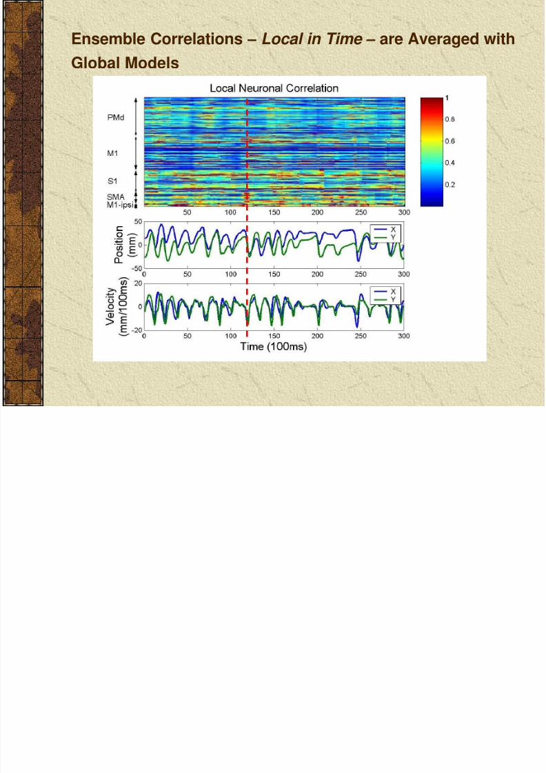
Ensemble Correlations – Local in Time – are Averaged withGlobal Models



Computational Models of Neural Intent

Two different levels of neurophysiology realism

Black Box models – no realism, function relation betweeninput desired response

Generative Models – minimal realism, state space modelsusing neuroscience elements



Signal Processing Approaches with BlackBox Modeling

Accessing 2 types of signals (cortical activity and behavior) leads us to ageneral class of I/O models.

Data for these models are rate codes obtained by binning spikes on 100msec windows.

Optimal FIR Filter – linear, feedforwardTDNN – nonlinear, feedforwardMultiple FIR filters – mixture of expertsRMLP – nonlinear, dynamic



Optimal Linear Model

Ten tap embedding with 105neuronsFor 1-D topology contains1,050 parameters (3,150)

The Wiener solution (coincideswith linear regression)



Optimal Linear ModelLet us assume that a M dimensional multiple time series isgenerated by a stationary stable vector autoregressive (VAR)model (b is a colum vector and W are MxM matrices ofcoefficients)

In matrix notation this can be written X=AZ+U

The multivariate least square estimation chooses the estimatorthat minimizes

)()(...)1()( 1 nu Ln xW n xW bn x L

1][

1)(][

1][

],...,[

)1(],...,[1)1(],...,,1[

)1(],...,,[

],...[

2

1

10

1

1

1

MTxU vec

x M L M Avec

MTx X vec

MxT uuU

xT ML Z Z Z x ML x x Z

ML MxW W b A

MxT x x X

T

T

T

Lnnn

L

T

)}(){()( 11 AZ X AZ X tr J T T

)(2)(2)( 11 Z ZZ

J T

))((ˆ 1 I Z ZZ T 1)( T T ZZ XZ A



Optimal Linear Model

Effectively we use a regularizedsolution

Normalized LMS with weightdecay is a simple starting point.

Four multiplies, one divide andtwo adds per weight update

)()()(

)()1( 2 n xnen x

nwnw

pw 1)( I R



Time-Delay Neural Network (TDNN)

The first layer is a bank of linearfilters followed by a nonlinearity.The number of delays to span Isecondy(n)= Σ wf(Σwx(n))Trained with backpropagationTopology contains a ten tapembedding and five hiddenPEs – 5,255 weights (1-D)

Principe, UF



Multiple Switching Local Models

Multiple adaptive filters that compete to win the modeling of a signalsegment.Structure is trained all together with normalized LMS/weight decayNeeds to be adapted for input-output modeling.We selected 10 FIR experts of order 10 (105 input channels)

d(n)



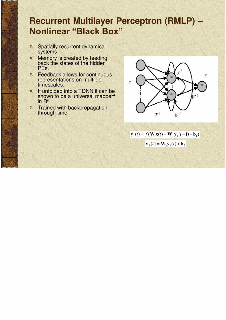
Recurrent Multilayer Perceptron (RMLP) – Nonlinear “Black Box”

Spatially recurrent dynamicalsystemsMemory is created by feedingback the states of the hiddenPEs.Feedback allows for continuous

representations on multipletimescales.If unfolded into a TDNN it can beshown to be a universal mapperin R n Trained with backpropagationthrough time

))1()(()( 1111 byWxWy t t f t f

2122 )()( byWy t t



Model Building Techniques

Train the adaptive system with neuronal firing rates (100 msec) as the input and hand position as thedesired signal.Training - 20,000 samples (~33 minutes of neuronalfiring)Freeze weights and present novel neuronal data.Testing - 3,000 samples – (5 minutes of neuronalfiring)



Results (Belle)

Signal to error ratio (dB) Correlation Coefficient

(average) (max) (average) (max)

LMS 0.8706 7.5097 0.6373 0.9528

Kalman 0.8987 8.8942 0.6137 0.9442

TDNN 1.1270 3.6090 0.4723 0.8525

Local Linear 1.4489 23.0830 0.7443 0.9748

RNN 1.6101 32.3934 0.6483 0.9852

Based on 5 minutes of test data, computed over 4 secwindows (training on 30 minutes)



Computing Sensitivities Through theModels

T

iit

T f t

T

t t

11

22

)()(

WDWDWx

y

))1()(()( 1111 byWxWy t t f t f

2122 )()( byWy t t

Feedforward RMLP Eqs.

General form of RMLPSensitivity

Feedforward Linear Eq.

General form of LinearSensitivity

Wx

y)(

)(t

t

)()( t t Wxy

Identify the neurons that affect the output the most.



Data Analysis : The Effect of Sensitive Neurons on Performance

0 20 40 60

-20

0

20

40

60

Hightest Sensitivity Neurons

0 20 40 60

-20

0

20

40

60

Middle Sensitivity Neurons

0 20 40 60

-20

0

20

40

60

Lowest Sensitivity Neurons

0 20 40 60 800

0.2

0.4

0.6

0.8

1

P r o

b a

b i l i t y

3D Error Radius (mm)

Movements (hits) of Test Trajectory

10 Highest Sensitivity

84 Intermediate Sensitivity

10 Lowest Sensitivity

All Neurons

0 20 40 60 80 100 1200

0.05

0.1

0.15

0.2

0.25

0.3

0.35

0.4

S e n s

i t i v i t y

Primate 1, Session 1

Neurons

93

192954

847

2645

104

Decay trend appears in allanimals and behavioral

paradigms



Cortical Contributions Belle Day 2

0 20 40

-20

0

20

40

60

Area 1

0 20 40

-20

0

20

40

60

Area 2

0 20 40

-20

0

20

40

60

Area 3

0 20 40

-20

0

20

40

60

Area 4

0 20 40

-20

0

20

40

60

Areas 12

0 20 40

-20

0

20

40

60

Areas 13

0 20 40

-20

0

20

40

60

Areas 14

0 20 40

-20

0

20

40

60

Areas 23

0 20 40

-20

0

20

40

60

Areas 24

0 20 40

-20

0

20

40

60

Areas 34

0 20 40

-20

0

20

40

60

Areas 123

0 20 40

-20

0

20

40

60

Areas 124

0 20 40

-20

0

20

40

60

Areas 134

0 20 40

-20

0

20

40

60

Areas 234

0 20 40

-20

0

20

40

60

Areas 1234

Area 1 PP

Area 2 M1

Area 3 PMd

Area 4 M1 (right)

Train 15 separate RMLPs with every combination of cortical input.



Is there enough information in spiketrains for modeling movement?

Analysis is based on the time embedded modelCorrelation with desired is based on a linear filter output foreach neuron

Utilize a non-stationary tracking algorithmParameters are updated by LMS

Build a spatial filterAdaptive in real timeSparse structure based on regularization for enablesselection



Adapted by LMS Adapted by on-line LAR(Kim et. al., MLSP , 2004)

Architecture

x1(n) z-1

z-1

y1(n) w11

w1 L

/ /

x M (n) z-1

z-1

y M (n) w M 1

w ML

/ /

…

y2(n)

…

c1

c M

)(ˆ

nd c2



Application to BMI Data – TrackingPerformance

A li i BMI D N l



Application to BMI Data – NeuronalSubset Selection

HandTrajectory

(z)

NeuronalChannelIndex

EarlyPart

LatePart



Generative Models for BMIs

Use partial information about the physiological system, normallyin the form of states.

They can be either applied to binned data or to spike trainsdirectly.

Here we will only cover the spike train implementations.

Difficulty of spike train Analysis:Spike trains are point processes , i.e. all the information is contained

in the timing of events, not in the amplitude fo the signals!



Build an adaptive signal processing framework forBMI decoding in the spike domain.

Features of Spike domain analysis

Binning window size is not a concernPreserve the randomness of the neuron behavior. Provide more understanding of neuron physiology (tuning) andinteractions at the cell assembly levelInfer kinematics onlineDeal with nonstationary

More computation with millisecond time resolution

Goal



Recursive Bayesian Approach

),~

(~

t t n X H Z t t

State Time-seriesmodel cont. observ.

Prediction),(

~11 t t t t v X F X

Updating

t Z

P(state|observation)



Recursive Bayesian approach

State space representation

First equation ( system model ) defines a first order Markov process.Second equation ( observation model ) defines the likelihood of the

observations p(z t|x t) . The problem is completely defined by theprior distribution p(x 0).

Although the posterior distribution p(x 0:t |u 1:t,z 1:t) constitutes thecomplete solution, the filtering density p(x

t|u

1:t, z

1:t) is normally

used for on-line problems.The general solution methodology is to integrate over the unknown

variables (marginalization).

t t t t t

t t t

n xuh z

v x f x

),(

)(1

h



Recursive Bayesian approach

There are two stages to update the filtering density:Prediction (Chapman Kolmogorov)

System model p(x t|x t-1) propagates into the future the posterior density

Update

Uses Bayes rule to update the filtering density. The following equationsare needed in the solution.

11:11:1111:11:1 ),|()|(),|( t t t t t t t t t dx zu x p x x p zu x p

),|(),|(),|(

),|(1:1

1:11:1:1:1

t t t

t t t t t t t t t zuu p

z x x pu x z p zu x p

1111111111 )()()|(),|()|( t t t t t t t t t t t t t dvv p xv xdv xv p xv x p x x p

t t t t t t t t t dnn pn xuh zu x z p )()),((),|(

t t t t t t t t t t dxu z x pu x z pu z z p ),|(),|(),|( 1:11:11:1



State estimation framework for BMI decoding

Tuning function

Kinematics

state

Neural Tuning

functionMulti-spike trains

observation

xk k-1xk F k-1v= ( ),

k x

k z

k H

k n= )( ,

0 0.2 0.4 0.6 0.8 1 1.2 1.4 1.6 1.8 2

x 105

0

0.1

0.2

0.3

0.4

0.5

0.6

0.7

0.8

0.9

1

time

s p

i k e

0 0.2 0.4 0.6 0.8 1 1.2 1.4 1.6 1.8 2

5

-1.5

-1

-0.5

0

0.5

1

1.5

time(ms)

v e

l o c

i t y

Decoding

Kinematic dynamic model

Key Idea : work with the probability of spike firing which is a

continuous random variable



Kalman filter for BMI decoding

KinematicState

Neuron tuningfunction Firing rate

ContinuousObservation

P(state|observation)Prediction

Updating

Gaussian

Linea

r

Linear

[Wu et al. 2006]

For Gaussian noises and linear prediction and observation models, thereis an analytic solution called the Kalman Filter.

Particle Filter for BMI decoding



Particle Filter for BMI decoding

KinematicState

Neuron tuningfunction Firing rate

ContinuousObservation

P(state|observation)Prediction

Updating

nonGaussianLinear

Exponential

[Brockwell et al. 2004]

In general the integrals need to be approximated by sums using

Monte Carlo integration with a set of samples drawn from theposterior distribution of the model parameters.



Step 2- Tuning Function Estimation

Neural firing Model

Assumption :

generation of the spikes depends only on the kinematic

vector we choose.

Linearfilter

nonlinear f Poissonmodel

velocity spikes

)( t t vk f

)( t t Poissonspike



Step 2- Linear Filter Estimation

Spike Triggered Average (STA)

Geometry interpretation][)][(

|1 v E I vv E k

spikev

T

-30 -20 -10 0 10 20 30-25

-20

-15

-10

-5

0

5

10

15

20

25

1st Principal Component

2 n d P r i n c

i p a

l C o m p o n e n

t

neuron 72: VpS PCA

VpVpS

1st Princi al com onent

2n

d P r i n

c i p

al c

om p on

en

t



Step 2- Nonlinear f estimation

Step 2- Diversity of neural nonlinear properties



Step 2- Diversity of neural nonlinear properties

Ref: Paradoxical cold

[Hensel et al. 1959]

Step 2- Estimated firing probability and



p g p ygenerated spikes

Step 3: Sequential Estimation Algorithm for



Step 3: Sequential Estimation Algorithm forPoint Process Filtering

Consider the neuron as an inhomogenous Poisson point process

Observing N(t) spikes in an interval T, the posterior of the spikemodel is

The probability of observing an event in t is

And the one step prediction density (Chapman-Kolmogorov)

The posterior of the state vector, given an observation N

}exp{)( k k k vk t

t t t t t N t t N

t t t t t

))(),(),(|1)()(Pr(lim))(),(),(|(

0

HθxHθx

)),|(exp()),|((),|( t t t t N P k k k N

k k k k k k k HxHxHx

)|()|(),|(

),|(k k

k k k k k k k k N p

p N P N p

HHxHx

Hx

11111 ),|(),|()|( k k k k k k k k k d N p p p xHxHxxHx

Step 3: Sequential Estimation Algorithm forS

N i

ik

ik w 1:0 },{x S

N i

ik

ik w 1:0 },{x S

N i

ik

ik w 1:0 },{x S

N i

ik

ik w 1:0 },{x



p q gPoint Process Filtering

Monte Carlo Methods are used to estimate the integral. Letrepresent a random measure on the posterior density, and represent

the proposed density by

The posterior density can then be approximated by

Generating samples from using the principle of Importance

sampling

By MLE we can find the maximum or use direct estimation with kernels

of mean and variance

)|( :1:0 k k N q x

N

i

i t t it t t x xk w N x p1

:0:0:1:0 ),()|(

S N

iik

ik w 1:0 },{x

),|()|()|(

)|()|(

1

11

:1:0

:1:0

k ik

ik

ik

ik

ik k i

k k

ik

k i

k ik N q

p N pw

N q N p

wxx

xxxxx

S N

i

ik

ik k k N p

1

~)|( xxx ))()(()|(

~

1

~T

k ik

N

i

k ik

ik k k

S

N pV xxxxx

)|( :1:0 k k N q x



Posterior density at a time index

-2.5 -2 -1.5 -1 -0.5 0 0.50

0.05

0.1

0.15

0.2

0.25

0.3

0.35

velocity

p r o

b a

b i l i t y

pdf at time index 45.092s

posterior density

desired velocityvelocity by seq. estimation (collapse)velocity by seq. estimation (MLE)velocity by adaptive filtering



Step 3: Causality concerns

0 0. 2 0. 4 0. 6 0. 8 1 1. 2 1. 4 1. 6 1. 8 2

x 105

0

0.1

0.2

0.3

0.4

0.5

0.6

0.7

0.8

0.9

1

time

s p

i k e

0 0.2 0.4 0.6 0.8 1 1.2 1.4 1.6 1.8 2

5

-1.5

-1

-0.5

0

0.5

1

1.5

time ms

v e

l o c

i t y

1,02);( )

)())(|(

(log))(|())(()(spike X

KX spike spike plagKX spike p

lagKX spike plagKX plag I

lag

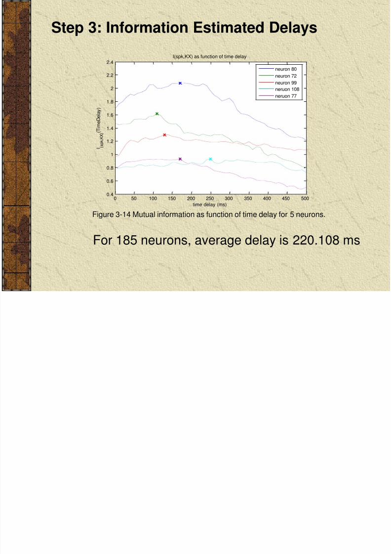
S 3 I f i E i d D l



For 185 neurons, average delay is 220.108 ms

0 50 100 150 200 250 300 350 400 450 5000.4

0.6

0.8

1

1.2

1.4

1.6

1.8

2

2.2

2.4

time delay (ms)

I ( s p k , K

X ) ( T

i m e

D e

l a y

)

I(spk,KX) as function of time delay

neuron 80neuron 72neuron 99neruon 108neruon 77

Figure 3-14 Mutual information as function of time delay for 5 neurons.

Step 3: Information Estimated Delays

Step 4:



Step 4:Monte Carlo sequential kinematics estimation

)(i

it t

X k f

KinematicState

Neural Tuningfunction spike trains

Prediction

it

it t

it v X F X 11

Updating

)|( )(1

it

jt

it

it N pww

)( j

t N

NonGaussian

P(state|observation) N

i

it t

it

jt t x xk w N x p

1:0:0

)(:1:0 )()|(

N

i

ik k

ik k k k W N p

1:1 )()|( xxx

Reconstruct the kinematics from neuron spike



trains

650 700 750 800-30

-20

-10

0

10

t

Px

650 700 750 800-40

-20

0

20

40

t

Py

650 700 750 800-2

-1

0

1

t

Vx

650 700 750 800-2

0

2

t

Vy

650 700 750 800-0.1

0

0.1

0.2

0.3

t

Ax

650 700 750 800-0.1

0

0.1

0.2

0.3

t

Ay

desiredcc exp =0.7002

cc MLE=0.69188


cc MLE=0.040027


cc MLE=0.91162


cc MLE=0.8151


cc MLE=0.95376

es recc exp =0.80243

cc MLE=0.67264

R lt i



Table 3-2 Correlation Coefficients between the Desired Kinematics and theReconstructions

CCPosition Velocity Acceleration

x y x y x y

Expectation 0.8161 0.8730 0.7856 0.8133 0.5066 0.4851

MLE 0.7750 0.8512 0.7707 0.7901 0.4795 0.4775

Table 3-3 Correlation Coefficient Evaluated by the Sliding Window

CC

Position Velocity Acceleration

x y x y x y

Expectation0.840100.0738

0.89450.0477

0.79440.0578

0.81420.0658

0.52560.0658

0.44600.1495

MLE 0.79840.0963 0.87210.0675 0.78050.0491 0.79180.0710 0.49500.0430 0.44710.1399

Results comparison

[Sanchez, 2004]



Conclusion

Our results and those from other laboratories show it is possible toextract intent of movement for trajectories from multielectrode arraydata.The current results are very promising, but the setups have limiteddifficulty, and the performance seems to have reached a ceiling at anuncomfortable CC < 0.9Recently, spike based methods are being developed in the hope ofimproving performance. But difficulties in these models are many.Experimental paradigms to move the field from the present level needto address issues of:

Training (no desired response in paraplegic)How to cope with coarse sampling of the neural populationHow to include more neurophysiology knowledge in the design

Survey Bmis 2011

Documents

Transcript of Survey Bmis 2011