Surface Water Temperature Modeling 6B.A: Surface Water Temperature Modeling . Final LTO EIS 6B.A-3 ....
609
Appendix 6B.A: Surface Water Temperature Modeling Final LTO EIS 6B.A-1 Appendix 6B, Section A 1 2 3 4 5 6 7 8 9 10 11 12 13 14 15 16 17 18 19 20 21 22 23 24 25 26 27 28 29 30 31 32 33 34 35 36 37 38 Surface Water Temperature Modeling This appendix provides information about the methods and assumptions used for the Coordinated Long-Term Operation of the Central Valley Project (CVP) and State Water Project (SWP) Environmental Impact Statement (EIS) analysis on surface water temperature. The appendix also provides temperature model results and interpretation methods used for the impacts analysis and descriptions. Additional information pertaining to the development of the analytical tools, incorporating climate change, and the use of input data from other models, is also provided. This appendix is organized into three sections that are briefly described below: • Appendix 6B, Section A: Surface Water Temperature Modeling Methodology, Simulations, and Assumptions – The water quality impacts analysis uses the HEC-5Q and Reclamation Monthly Temperature models to assess and quantify effects of the alternatives on the environment. This section provides information about the overall analytical framework linkages with other models. – This section provides a brief description of the assumptions for the surface water temperature model simulations of the No Action Alternative, Second Basis of Comparison, and other alternatives. • Appendix 6B, Section B: Surface Water Temperature Modeling Results – This section provides model outputs and a description of the model simulation output formats used in the analysis and interpretation of modeling results for the alternatives impacts assessment. • Appendix 6B, Section C: HEC-5Q Model Update for Surface Water Temperature Modeling – This section provides a detailed description of the compilation and updates of the HEC-5Q models performed during development of the EIS for the Trinity-Sacramento, American, and Stanislaus Rivers. 6B.A.1 Surface Water Temperature Modeling Methodology This section summarizes the surface water temperature modeling methodology used for the No Action Alternative, Second Basis of Comparison, and other alternatives. It describes how temperature modeling fits into the overall analytical framework and contains descriptions of the key analytical and numerical tools and approaches used in the quantitative evaluation of the alternatives. In the evaluation of the No Action Alternative, Second Basis of Comparison, and other alternatives, climate change assumptions at the Year 2030 are used to DWR-1085
-
Upload
nguyenhanh -
Category
Documents
-
view
217 -
download
1
Transcript of Surface Water Temperature Modeling 6B.A: Surface Water Temperature Modeling . Final LTO EIS 6B.A-3 ....

Appendix 6B.A: Surface Water Temperature Modeling
Final LTO EIS 6B.A-1
Appendix 6B, Section A 1
2
3 4 5 6 7 8 9
10 11
12 13
14 15 16 17
18 19 20
21
22 23 24
25 26
27 28 29
30 31
32 33 34 35 36
37 38
Surface Water Temperature Modeling This appendix provides information about the methods and assumptions used for the Coordinated Long-Term Operation of the Central Valley Project (CVP) and State Water Project (SWP) Environmental Impact Statement (EIS) analysis on surface water temperature. The appendix also provides temperature model results and interpretation methods used for the impacts analysis and descriptions. Additional information pertaining to the development of the analytical tools, incorporating climate change, and the use of input data from other models, is also provided. This appendix is organized into three sections that are briefly described below:
• Appendix 6B, Section A: Surface Water Temperature Modeling Methodology,Simulations, and Assumptions
– The water quality impacts analysis uses the HEC-5Q and ReclamationMonthly Temperature models to assess and quantify effects of thealternatives on the environment. This section provides information aboutthe overall analytical framework linkages with other models.
– This section provides a brief description of the assumptions for the surfacewater temperature model simulations of the No Action Alternative,Second Basis of Comparison, and other alternatives.
• Appendix 6B, Section B: Surface Water Temperature Modeling Results
– This section provides model outputs and a description of the modelsimulation output formats used in the analysis and interpretation ofmodeling results for the alternatives impacts assessment.
• Appendix 6B, Section C: HEC-5Q Model Update for Surface WaterTemperature Modeling
– This section provides a detailed description of the compilation and updatesof the HEC-5Q models performed during development of the EIS for theTrinity-Sacramento, American, and Stanislaus Rivers.
6B.A.1 Surface Water Temperature Modeling Methodology
This section summarizes the surface water temperature modeling methodology used for the No Action Alternative, Second Basis of Comparison, and other alternatives. It describes how temperature modeling fits into the overall analytical framework and contains descriptions of the key analytical and numerical tools and approaches used in the quantitative evaluation of the alternatives.
In the evaluation of the No Action Alternative, Second Basis of Comparison, and other alternatives, climate change assumptions at the Year 2030 are used to
DWR-1085

Appendix 6B.A: Surface Water Temperature Modeling
6B.A-2 Final LTO EIS
develop modified climate input files for the temperature models. The modeling 1 2
3 4 5 6 7 8 9
10 11 12 13 14 15 16 17 18
19 20 21 22 23 24 25 26 27 28 29 30 31
32 33 34
35 36
37 38 39 40 41 42
assumptions are provided in Section 6B.A.2.
6B.A.1.1 Overview of the Modeling Approach To support the water quality and aquatic resources impact analyses of the alternatives, modeling of surface water temperature in the Central Valley is necessary to evaluate changes to conditions affecting surface water temperatures in rivers that are affected by SWP and CVP operations. Two different surface water temperature modeling tools were used for the analysis. The HEC-5Q model simulated daily temperatures for the Trinity River (downstream of Lewiston Dam), Sacramento River (from Keswick Dam to the Feather River confluence), American River (from Nimbus Dam to Sacramento River confluence), and Stanislaus River (from New Melones Dam to the confluence with San Joaquin River). The Reclamation Temperature Model was used for simulating monthly temperatures for the Feather and Lower Sacramento (from the Feather River confluence to Freeport) rivers. Both models used CalSim II outputs as stream flow and reservoir storage inputs. The results from these models are used to inform the understanding of effects on the surface water temperature of each individual alternative considered in the EIS.
6B.A.1.1.1 HEC-5Q Over the past 15 years, various temperature models were developed to simulate temperature conditions on the rivers affected by CVP and SWP operations (Sacramento River Water Quality Model [SRWQM], San Joaquin River HEC-5Q model) (Reclamation 2008). Recently, these models were compiled and updated into a single modeling package hereafter referred to as the HEC-5Q model. Further updates were performed under the EIS modeling that included improved meteorological data and subsequent validation of the Sacramento and American River models, implementation of the Folsom Temperature Control Devices and low-level outlet, implementation of the Trinity River auxiliary outlet, improved temperature targeting for the Shasta and Folsom Dams, as well as improved documentation and streamlining of the models as well as improved integration with the CalSim II model.
Section 6B.C.4 of this appendix is consistent with the technical memorandum submitted to Reclamation that documented changes in the HEC-5Q compilation and updates for the temperature models.
The HEC-5Q model contains three separate models that simulate reservoir and river temperatures:
• The Trinity River from Trinity Dam to below Lewiston Dam and the Sacramento River from Shasta Dam to the Feather River confluence. Reservoir temperatures are simulated for Trinity Lake, Lewiston Reservoir, Shasta Lake, Keswick Reservoir, and Black Butte Reservoir (see Figure 6B.A.1 for a schematic of the Trinity-Sacramento River HEC-5Q model).

Appendix 6B.A: Surface Water Temperature Modeling
Final LTO EIS 6B.A-3
• The American River from Folsom Dam to the confluence with the Sacramento 1 2 3 4
5 6 7 8 9
10 11 12 13 14 15
16 17 18 19 20 21 22 23 24 25 26 27 28 29 30 31 32 33 34
35 36 37 38
39 40 41
River. Reservoir temperatures were simulated for Folsom Lake and Lake Natoma (see Figure 6B.A.2 for a schematic of the American River HEC-5Q model).
• The Stanislaus River from upstream of New Melones Reservoir to the confluence with the San Joaquin River and the lower San Joaquin River from the Stanislaus River confluence to below Vernalis. Reservoir temperatures were simulated for New Melones Reservoir (see Figure 6B.A.3 for a schematic of the Stanislaus River HEC-5Q model).
The HEC-5Q model was developed using integrated HEC-5 and HEC-5Q models. The HEC-5 component of the model simulates daily reservoir and river flow operations from monthly CalSim II data that are disaggregated to daily data. The HEC-5Q component simulates mean daily reservoir and river temperatures based on the daily flow inputs and meteorological parameters specified on a 6-hour time step.
6B.A.1.1.2 Reclamation Temperature Model The Reclamation Temperature Model includes reservoir and stream temperature models that simulate monthly reservoir and stream temperatures used for evaluating the effects of CVP and SWP project operations on mean monthly water temperatures in the basin (Reclamation 2008). The model simulates temperatures in seven major reservoirs (Trinity Lake, Whiskeytown Reservoir, Shasta Lake, Oroville Reservoir, Folsom Lake, New Melones Reservoir, and Tulloch Reservoir), four downstream regulating reservoirs (Lewiston, Keswick, and Goodwin reservoirs; Lake Natoma), and five main river systems (Trinity, Sacramento, Feather, American, and Stanislaus rivers). The river component of the Reclamation Temperature Model calculates temperature changes in the regulating reservoirs, below the main reservoirs. With regulating reservoir release temperature as the initial river temperature, the river model computes temperatures at several locations along the rivers. The calculation points for river temperatures generally coincide with tributary inflow locations. The model is one-dimensional in the longitudinal direction and assumes fully mixed river cross sections. The effect of tributary inflow on river temperature is computed by mass balance calculation. The river temperature calculations are based on regulating reservoir release temperatures, river flows, and climatic data.
For the EIS, the Reclamation Temperature Model was used for the Feather River and lower Sacramento River from the Feather River confluence to Freeport. Sacramento, Trinity, American, and Stanislaus rivers temperature effects were analyzed using the daily HEC-5Q models described in the previous section.
For more information on the Reclamation Temperature Model, see Appendix H of the Reclamation’s 2008 Operation Criteria and Plan (OCAP) Biological Assessment (BA) (Reclamation 2008).

Appendix 6B.A: Surface Water Temperature Modeling
6B.A-4 Final LTO EIS
6B.A.2 Surface Water Temperature Modeling 1 2
3 4 5
6 7 8 9
10 11
12 13
14 15
16
17 18
19
20 21
22 23 24 25 26 27 28
29
30 31 32 33
Simulations and Assumptions
This section describes the assumptions for the HEC-5Q and Reclamation Temperature Model monthly temperature simulations of the No Action Alternative, Second Basis of Comparison, and Alternatives 1 through 5.
The following model simulations were performed as the basis of evaluating the impacts of Alternatives 1 through 5 as compared to the No Action Alternative, and the No Action Alternative and Alternatives 1 through 5 as compared to the Second Basis of Comparison:
• No Action Alternative • Second Basis of Comparison
• Alternative 1 – for simulation purposes, considered the same as Second Basis of Comparison
• Alternative 2 – for simulation purposes, considered the same as No Action Alternative
• Alternative 3
• Alternative 4 – for simulation purposes, considered the same as Second Basis of Comparison.
• Alternative 5
Assumptions for each of these alternatives were developed with the surface water modeling tools and are described in Appendix 5A, Section B.
Alternative 1 modeling assumptions are the same as the Second Basis of Comparison and Alternative 2 modeling assumptions are the same as the No Action Alternative; therefore, the assumptions for those alternatives are not discussed separately in this document. The general modeling assumptions described below pertain to the model runs for the No Action Alternative, Second Basis of Comparison, and Alternatives 1 through 5.
6B.A.2.1 Input Storage and Streamflow
6B.A.2.1.1 HEC-5Q Monthly flows simulated by the CalSim II model for an 82-year period (water years 1922 through 2003) are used as input to HEC-5Q. Temporal downscaling is performed1 on the CalSim II monthly average tributary flows to convert them to
1 A constant daily flow that is equivalent to monthly average flow simulated in CalSim II is assumed throughout the month for each month of the 82-year CalSim II simulation period. An exception to this is the inflow timeseries to Trinity, Shasta, and New Melones reservoirs, where monthly average inflows are downscaled to a daily timestep by fitting to a cubic-spline. This allows simulation of a daily varying inflow into the reservoirs with a smooth transition between the individual months, while assuming the same monthly volume of inflow consistent with CalSim II.

Appendix 6B.A: Surface Water Temperature Modeling
daily average flows for HEC-5Q input using a pre-processing tool (see Tables 6B.A.1 to 6B.A.3 for a list of all of the CalSim II inputs).
1 2
Table 6B.A.1 CalSim II Input Mapping with Trinity-Sacramento River HEC-5Q Model 3 HEC-5Q
Control Point Number
HEC-5Q Control Point Name Input Types CalSim II Node
340 Trinity Reservoir
Storage Inflow
Outflow Evaporation
S1 I1
C1+F1 E1
330 Lewiston Reservoir Inflow
Diversion I100 D100
240 Whiskeytown Reservoir
Storage Inflow
Outflow Evaporation
S3 I3
C3+F3 E3
220 Shasta Reservoir
Storage Inflow
Outflow Evaporation
S4 I4
C4+F4 E4
200 Keswick Reservoir Evaporation E5
180 Sacramento River below Clear Creek Confluence
Diversion C5-C104
178 Sacramento River below Cow Creek Confluence
Inflow C10801
176 Sacramento River below Cottonwood Creek Confluence
Inflow C10802
172 Sacramento River below Battle Creek Confluence
Inflow C10803
170 Sacramento River at Bend Bridge
Inflow Diversion
I109+R109 D109
160 Sacramento River above Red Bluff Diversion Dam
Inflow Diversion
C11001+I112 D112
150 Sacramento River below Woodson Bridge
Inflow Diversion
C11305+C11301+R113+R114A+R114B+R114C D113A+D113B
140 Sacramento River at GCID Diversion D114
1136 Black Butte Reservoir
Storage Inflow
Outflow Diversion
S42 I42+C41 C42+F42 E42+D42
Final LTO EIS 6B.A-5

Appendix 6B.A: Surface Water Temperature Modeling
6B.A-6 Final LTO EIS
HEC-5Q Control Point
Number HEC-5Q Control
Point Name Input Types CalSim II Node
1134 Stony Creek Diversions Diversion C42-C142A
1132 Stony Creek Confluence Inflow C11501
132 Sacramento River at Ord Ferry Diversion D117
130 Sacramento River at Butte City
Inflow Diversion
I118 I118+C115-C118-D117
128 Sacramento River above Moultin Weir
Inflow Diversion
I123+c17603 C118+I123+C17603-C124
126 Sacramento River at Moultin Weir Diversion D124
120 Sacramento River at Colusa Weir Diversion D125
116 Sacramento River at Tisdale Weir Diversion D126
114 Sacramento River above Knights Landing
Diversion C126-C129
112 Sacramento River at Knights Landing Diversion C129-C134
365 Butte Creek BP3 Diversion C136B-R137-R135A-R135B-C217A
Table 6B.A.2 CalSim II Input Mapping with American River HEC-5Q Model 1 HEC-5Q Control Point
Number
HEC-5Q Control Point Name Input Types CalSim II Node
590 Folsom Reservoir
Storage Inflow
Outflow Diversion
S8 C300+I8 C8+F8 E8+D8
580 Natoma Reservoir Storage
Diversion S9
D9+E9-I9
572
American River above City of Sacramento Diversion
Diversion GS66-I302
570 American River at City of Sacramento Diversion
Diversion D302

Appendix 6B.A: Surface Water Temperature Modeling
Final LTO EIS 6B.A-7
Table 6B.A.3 CalSim II Input Mapping with Stanislaus River HEC-5Q Model 1
2 3 4 5 6 7
8 9
10 11
HEC-5Q Control Point
Number HEC-5Q Control
Point Name Input Types CalSim II Node
240 New Melones Reservoir
Storage Inflow
Outflow Evaporation
S10 I10
C10+F10 E10
220 Tulloch Reservoir Storage Inflow
Diversion
S76 I76 E76
200 Goodwin Reservoir Inflow
Diversion I520
C76-C520
160 Stanislaus River at Knights Ferry Diversion C520-C528
150 Stanislaus River at Orange Blossom Bridge
Diversion C520-C528
140 Stanislaus River at Oakdale Highway 120 Bridge
Diversion C520-C528
130 Stanislaus River at Riverbank Bridge Diversion C520-C528
120 Stanislaus River at McHenry Bridge Diversion C520-C528
110 Stanislaus River at Ripon Gage Diversion C520-C528
400
San Joaquin River above Stanislaus River Confluence Dummy Reservoir
Diversion C620+C545+C528-C644
98 San Joaquin River at Vernalis Diversion C620+C545+C528-C644
6B.A.2.1.2 Reclamation Temperature Model Monthly flows that were simulated by the CalSim II model for an 81-year period (January 1922 to December 2002) are used as input to the model. Because of the CalSim II model’s complex structure, where applicable, flow arcs were combined at the appropriate temperature nodes to ensure compatibility with the Reclamation Temperature Model.
6B.A.2.2 Climate Change Assumptions When simulating alternatives with climate change, some of the inputs to the temperature models must be modified. This section presents the assumptions and approaches used for modifying meteorological and inflow temperatures in the

Appendix 6B.A: Surface Water Temperature Modeling
6B.A-8 Final LTO EIS
temperature models. For the alternative simulations, climate assumptions were 1 2 3 4 5
6 7 8 9
10 11 12 13
14 15 16 17 18 19 20 21 22 23 24 25 26 27
28 29 30 31 32 33 34 35 36 37
38 39 40 41 42
established around Year 2030. Therefore, to be consistent with the other water supply and economics models, the climate input data for HEC-5Q and Reclamation Temperature Model were modified to represent approximate conditions at Year 2030.
6B.A.2.2.1 HEC-5Q HEC-5Q requires meteorological inputs specified in the form of equilibrium temperatures, exchange rates, shortwave radiation and wind speed. The exchange rates and equilibrium temperatures are computed from hourly observed data at the Gerber gauging station. Considering the uncertainties associated with climate change impacts, it was assumed that the equilibrium temperature inputs derived from observed data would be modified by the change in daily average air temperature projected under the climate change scenarios.
The inflow temperatures in HEC-5Q are specified as seasonal curve fit values with diurnal variations superimposed as a function of heat exchange parameters. The seasonal temperature values are derived based on the observed flows and temperatures for each inflow. HEC-5Q superimposes diurnal variations on the seasonal values specified using the heat exchange parameter inputs. The diurnal variations are superimposed by adjusting the equilibrium temperature to reflect the inflow location environment and scaling it based on the heat exchange rate scaling factor and the weighting factor for emphasis on the seasonal values specified. In this fashion, any climate change effects accounted for in the equilibrium temperature are translated to the changes in inflow temperatures in the HEC-5Q. Therefore, for the climate change scenarios, only the equilibrium temperatures were adjusted for the projected change in temperature, and these influence the inflow temperatures; however, independent inflow temperature inputs were not changed.
6B.A.2.2.2 Reclamation Temperature Model The Reclamation Temperature Model requires mean monthly meteorological inputs of air and equilibrium temperature and heat exchange rates. The heat exchange rates and equilibrium temperatures are computed from the mean monthly air temperature data and long-term estimates of solar radiation, relative humidity, wind speed, cloud cover, solar reflectivity, and river shading. Considering the uncertainties associated with climate change impacts, it was assumed that the equilibrium temperature and heat exchange rate inputs would be modified by the change in mean monthly air temperature in the climate change scenarios.
Reservoir inflow temperatures were derived from the available record of observed data and averaged by month. The mean monthly inflow temperatures are then repeated for each study year. For alternatives modeled with climate change, the inflow temperatures were modified based on the projected long-term average change in mean annual air temperature for each month.

Appendix 6B.A: Surface Water Temperature Modeling
Final LTO EIS 6B.A-9
6B.A.3 Reference 1
2 3 4 5
Reclamation (Bureau of Reclamation). 2008. 2008 Central Valley Project and State Water Project Operations Criteria and Plan Biological Assessment, Appendix H Reclamation Temperature Model and SRWQM Temperature Model.

Appendix 6B.A: Surface Water Temperature Modeling
6B.A-10 Final LTO EIS
Trinity Reservoir
Trinity River Above Lewiston
Lewiston Reservoir
340
330
320
300Trinity River Below Lewiston
242 240Clear Creek Power Plant
232
WhiskeytownReservoir
Clear Creek Below Whiskeytown
220
210
200
Shasta Reservoir
Sacramento River Above Keswick
Keswick Reservoir
180
178
Sacramento River at Clear Creek Confluence
Sacramento River below Cow Creek Confluence
174 Sacramento River below Cottonwood Creek Confluence
172 Sacramento River below Battle Creek Confluence
170Sacramento River at
Bend Bridge
160
158
Sacramento River at Red Bluff Diversion Dam
Red Bluff Diversion Dam
150 Sacramento River below Woodson Bridge
140 Sacramento River at GCID
1321136
1134 1132Sacramento River at
Ord Ferry
130
Black Butte Reservoir
Stony Creek Diversions
Stony Creek Confluence
Sacramento River at Butte City
176
Cottonwood Creek Dummy Reservoir
244
Clear Creek Power Plant
Dummy Reservoir
242
Spring Creek Power Plant
214Spring Creek Power
Plant Dummy Reservoir
128Sacramento River above Moultin Weir
126Sacramento River at Moultin Weir
120Sacramento River at Colusa Weir
118Sacramento River above Tisdale Weir
116Sacramento River at Tisdale Weir
114Sacramento River above Knights Landing
112Sacramento River at Knights Landing
110Sacramento River above Sutter Bypass
106
Sacramento River above Sutter Bypass
Dummy Reservoir
102Sutter Bypass Sacramento
River Confluence
100Sacramento River at Feather River Confluence
380
375
370
365
362
360
355
352
350
390
385
Ord Ferry Spills
Butte Creek BP1
Moultin Weir
Butte Creek BP2
Colusa Weir
Butte Creek BP3
Butte-Sutter
Tisdale Weir
Sutter BP1
Sutter BP2
Sutter Bypass above Sacramento River Dummy Reservoir
1 Figure 6B.A.1 Schematic of Trinity-Sacramento River HEC-5Q Model 2

Appendix 6B.A: Surface Water Temperature Modeling
Final LTO EIS 6B.A-11
Folsom Reservoir 590
582American River Above Natoma
580Natoma
Reservoir
578American River below Natoma
572American River upstream of City of Sacramento Diversion
570American River at City of Sacramento Diversion
80American River at Sacramento
River Confluence1 Figure 6B.A.2 Schematic of American River HEC-5Q Model 2

Appendix 6B.A: Surface Water Temperature Modeling
6B.A-12 Final LTO EIS
330Middle Fork Stanislaus
River Dummy Reservoir
318
Collierville Powerhouse Dummy Reservoir 320
Middle Fork Stanislaus River above Stanislaus Powerhouse
310Stanislaus Powerhouse
Dummy Reservoir
300
290
Middle Fork Stanislaus River above New Melones Reservoir #1
Middle Fork Stanislaus River above New Melones Reservoir #2
New MelonesReservoir 240
230Stanislaus River above Tulloch Reservoir
Tulloch Reservoir 220
210Stanislaus River above Goodwin Reservoir
Goodwin Reservoir 200
198Stanislaus River above Goodwin Reservoir
160Stanislaus River at Knights Ferry
150Stanislaus River at Orange Blossom Bridge
140Stanislaus River at Oakdale Highway 120 Bridge
130Stanislaus River at Riverbank Bridge
120Stanislaus River at McHenry Bridge
110 Stanislaus River at Ripon Gage
100
San Joaquin River at Stanislaus River
Confluence
98
San Joaquin River at Vernalis
98
San Joaquin River at Mossdale
400San Joaquin River above
Stanislaus River Confluence Dummy Reservoir
1 Figure 6B.A.3 Schematic of Stanislaus River HEC-5Q Model 2

Appendix 6B.B: Surface Water Temperature Modeling Results
Appendix 6B, Section B 1
2
3
4 5 6 7 8
9 10
11 12 13 14
15 16 17
18
19 20 21
22 23
24 25 26
27
28 29 30 31
32
33 34 35 36 37
Surface Water Temperature Modeling Results This appendix provides information about the methods and assumptions used for the Coordinated Long-Term Operation of the Central Valley Project (CVP) and State Water Project (SWP) Environmental Impact Statement (EIS) analysis on surface water temperature. The appendix is organized into three sections that are briefly described below:
• Appendix 6B, Section A: Surface Water Temperature Modeling Methodology,Simulations, and Assumptions
– The water quality impacts analysis uses the HEC-5Q and ReclamationMonthly Temperature models to assess and quantify effects of thealternatives on the environment. This section provides information aboutthe overall analytical framework linkages with other models.
– This section provides a brief description of the assumptions for the surfacewater temperature model simulations of the No Action Alternative,Second Basis of Comparison, and other alternatives.
• Appendix 6B, Section B: Surface Water Temperature Modeling Results
– This section provides model outputs and a description of the modelsimulation output formats used in the analysis and interpretation ofmodeling results for the alternatives impact assessment.
• Appendix 6B, Section C: HEC-5Q Model Update for Surface WaterTemperature Modeling
– This section provides a detailed description of the compilation and updatesof the HEC-5Q models performed during development of the EIS for theTrinity-Sacramento, American, and Stanislaus Rivers.
6B.B.1 Introduction
This section provides surface water temperature model (HEC-5Q and Reclamation Temperature Model) simulation results for alternatives evaluated for the EIS. The sections provided for each parameter include figures and tables in various formats to provide the reader with tools for multiple ways of analysis.
The different types of presentations are explained as follows:
• Probability of Exceedance Plots: Probability of exceedance plots provide thefrequency of occurrence of values of a parameter that exceed a referencevalue. For this appendix, the calculation of exceedance probability is done byranking the data. For example, for Shasta storage end-of-Septemberexceedance plot, Shasta storage values at the end of September for each
Final LTO EIS 6B.B-1

Appendix 6B.B: Surface Water Temperature Modeling Results
simulated year are sorted in ascending order. The smallest value would have a 1 2 3 4 5 6 7 8 9
10
11 12 13 14 15 16 17 18
19
20 21 22
23 24
25 26
27 28 29 30 31
32 33 34 35 36 37
38 39 40 41
probability of exceedance of 100 percent since all other values would be greater than that value; and the largest value would have a probability of exceedance of 0 percent. All of the values are plotted with probability of exceedance on the x-axis and the value of the parameter on the y-axis. Following the same example, if for one scenario, Shasta Lake end-of-September storage of 2,000 thousand acre-feet (TAF) corresponds to 80 percent probability, it implies that Shasta end-of-September storage is higher than 2,000 TAF in 80 percent of the years under the simulated conditions.
• Long-Term Average Summary and Year-Type-Based Statistics SummaryTables: These tables provide parameter values for each 10 o increment ofexceedance probability (rows) for each month (columns) as well as long-termand year-type averages (using the Sacramento Valley 40-30-30 Indexdeveloped by the State Water Resources Control Board for projected climateat Year 2030) for each month. For a few parameters, such as Delta outflow,annual total or average values are added to the tables (for volume and rates,respectively).
All plots and tables are prepared to accommodate following comparisons:
• No Action Alternative (with climate change and sea-level rise at Year 2030)compared to the Second Basis of Comparison (with climate change andsea-level rise at Year 2030)
• Alternatives (with climate change and sea-level rise at Year 2030) comparedto the No Action Alternative
• Alternatives (with climate change and sea-level rise at Year 2030) comparedto the Second Basis of Comparison
6B.B.1.1 Appropriate Use of Model Results The physical models developed and applied in the EIS analysis are generalized and simplified representations of a complex water resources system. A brief description of the appropriate use of the model results to compare two scenarios or to compare against threshold values or standards is presented below.
6B.B.1.1.1 Absolute vs. Relative Use of the Model Results The models are not predictive models (in how they are applied in this project), and therefore the results cannot be considered as absolute with and within a quantifiable confidence interval. The model results are only useful in a comparative analysis and can only serve as an indicator of condition (e.g., compliance with a standard) and of trend (e.g., generalized impacts).
6B.B.1.2 Appropriate Reporting Time-Step Due to the assumptions involved in the input data sets and model logic, care must be taken to select the most appropriate time-step for the reporting of model results. Sub-monthly (e.g., weekly or daily) reporting of model results is
6B.B-2 Final LTO EIS

Appendix 6B.B: Surface Water Temperature Modeling Results
i1 b2
63 4
a5 r6 a7 s8 (9
10 ti11 r12 i13 o14
15 a16 y17 d18 t19 y20 (21 i22 o23
24 f25 (26 a27 c28
29
30
•31 •32 •33 •34 •35 •36 •37 •38 •39 •40 •41
nappropriate for all models and the results should be presented on a monthly asis.
B.B.1.3 Statistical Comparisons Are Preferred Absolute differences computed at a point in time between model results from an lternative and a baseline to evaluate impacts is an inappropriate use of model esults (e.g., computing differences between the results from a baseline and an lternative for a particular day or month and year within the period of record of imulation). Likewise computing absolute differences between an alternative or a baseline) and a specific threshold value or standard is an inappropriate use of
model results. Statistics computed based on the absolute differences at a point in me (e.g., average of monthly differences) are an inappropriate use of model esults. By computing the absolute differences in this way, disregards the changes n antecedent conditions between individual scenarios and distorts the evaluation f impacts of a specific action.
Reporting seasonal patterns from long-term averages and water year-type verages is appropriate. Statistics computed based on long-term and water ear-type averages are an appropriate use of model results. Computing ifferences between long-term or water year type averages of model results from wo scenarios are appropriate. Care should be taken to use the appropriate water ear type for presenting water year-type average statistics of model results e.g., D1641 Sacramento River 40-30-30 index or San Joaquin River 60-20-20ndex based on climate modifications). For this study, water year-types are based n the projected climate and hydrology at Year 2030.
The most appropriate presentation of monthly and annual model results is in the orm of probability distributions and comparisons of probability distributions e.g., cumulative probabilities). If necessary, comparisons of model resultsgainst threshold or standard values should be limited to comparisons based on umulative probability distributions.
6B.B.2 Results
The results are presented in the following figures.
B.1. Trinity River below Lewiston Temperature B.2. Clear Creek below Whiskeytown Temperature B.3. Clear Creek at Igo Temperature B.4. Clear Creek at Mouth Temperature B.5. Sacramento River below Keswick Temperature B.6. Sacramento River at Balls Ferry Temperature B.7. Sacramento River at Jellys Ferry Temperature B.8. Sacramento River at Bend Bridge Temperature B.9. Sacramento River at Red Bluff Temperature B.10. Sacramento River at Hamilton City Temperature B.11. Sacramento River at Knights Landing Temperature
Final LTO EIS 6B.B-3
Appendix 6B.B: Surface Water Temperature Modeling Results
• B.12. American River below Nimbus Temperature 1 2 3 4 5 6 7 8 9
10 11 12
• B.13. American River at Watt Avenue Temperature• B.14. American River at Mouth Temperature• B.15. Stanislaus River below New Melones Temperature• B.16. Stanislaus River below Tulloch Temperature• B.17. Stanislaus River below Goodwin Temperature• B.18. Stanislaus River at Orange Blossom Bridge Temperature• B.19. Stanislaus River at Mouth Temperature• B.20. Feather River Low Flow Channel• B.21. Feather River at Robinson Riffle• B.22. Feather River at Gridley Bridge• B.23. Feather River at Mouth
6B.B-4 Final LTO EIS

B.1. Trinity River below Lewiston Temperature
Appendix 6B: Surface Water Temperature Modeling
Final LTO EIS 6B.B-5

Figure B-1-1. Trinity River below Lewiston Dam, October
Notes: 1) Exceedance probability is defined as the probability a given value will be exceeded in any one year. 2) All alternatives are simulated with projected hydrology and
sea level at Year 2030 conditions. 3) Model results for Alternatives 1, 4, and Second Basis of Comparison are the same, therefore Alternatives 1 and 4 results are not
presented. Qualitative differences, if applicable, are discussed in the text. 4) Model results for Alternative 2 and No Action Alternative are the same, therefore Alternative 2
results are not presented. Qualitative differences, if applicable, are discussed in the text.
34
36
38
40
42
44
46
48
50
52
54
56
58
60
62
64
0%10%20%30%40%50%60%70%80%90%100%
Exceedance Probability
No Action Alternative & Alternative 2 Second Basis of Comparison, Alternative 1, & Alternative 4
Alternative 3 Alternative 5
Mon
thly
Tem
pera
ture
(DE
G-F
)
Final LTO EIS 6B.B-6

Figure B-1-2. Trinity River below Lewiston Dam, November
Notes: 1) Exceedance probability is defined as the probability a given value will be exceeded in any one year. 2) All alternatives are simulated with projected hydrology and
sea level at Year 2030 conditions. 3) Model results for Alternatives 1, 4, and Second Basis of Comparison are the same, therefore Alternatives 1 and 4 results are not
presented. Qualitative differences, if applicable, are discussed in the text. 4) Model results for Alternative 2 and No Action Alternative are the same, therefore Alternative 2
results are not presented. Qualitative differences, if applicable, are discussed in the text.
34
36
38
40
42
44
46
48
50
52
54
56
58
60
62
64
0%10%20%30%40%50%60%70%80%90%100%
Exceedance Probability
No Action Alternative & Alternative 2 Second Basis of Comparison, Alternative 1, & Alternative 4
Alternative 3 Alternative 5
Mon
thly
Tem
pera
ture
(DE
G-F
)
Final LTO EIS 6B.B-7

Figure B-1-3. Trinity River below Lewiston Dam, December
Notes: 1) Exceedance probability is defined as the probability a given value will be exceeded in any one year. 2) All alternatives are simulated with projected hydrology and
sea level at Year 2030 conditions. 3) Model results for Alternatives 1, 4, and Second Basis of Comparison are the same, therefore Alternatives 1 and 4 results are not
presented. Qualitative differences, if applicable, are discussed in the text. 4) Model results for Alternative 2 and No Action Alternative are the same, therefore Alternative 2
results are not presented. Qualitative differences, if applicable, are discussed in the text.
34
36
38
40
42
44
46
48
50
52
54
56
58
60
62
64
0%10%20%30%40%50%60%70%80%90%100%
Exceedance Probability
No Action Alternative & Alternative 2 Second Basis of Comparison, Alternative 1, & Alternative 4
Alternative 3 Alternative 5
Mon
thly
Tem
pera
ture
(DE
G-F
)
Final LTO EIS 6B.B-8

Figure B-1-4. Trinity River below Lewiston Dam, January
Notes: 1) Exceedance probability is defined as the probability a given value will be exceeded in any one year. 2) All alternatives are simulated with projected hydrology and
sea level at Year 2030 conditions. 3) Model results for Alternatives 1, 4, and Second Basis of Comparison are the same, therefore Alternatives 1 and 4 results are not
presented. Qualitative differences, if applicable, are discussed in the text. 4) Model results for Alternative 2 and No Action Alternative are the same, therefore Alternative 2
results are not presented. Qualitative differences, if applicable, are discussed in the text.
34
36
38
40
42
44
46
48
50
52
54
56
58
60
62
64
0%10%20%30%40%50%60%70%80%90%100%
Exceedance Probability
No Action Alternative & Alternative 2 Second Basis of Comparison, Alternative 1, & Alternative 4
Alternative 3 Alternative 5
Mon
thly
Tem
pera
ture
(DE
G-F
)
Final LTO EIS 6B.B-9

Figure B-1-5. Trinity River below Lewiston Dam, February
Notes: 1) Exceedance probability is defined as the probability a given value will be exceeded in any one year. 2) All alternatives are simulated with projected hydrology and
sea level at Year 2030 conditions. 3) Model results for Alternatives 1, 4, and Second Basis of Comparison are the same, therefore Alternatives 1 and 4 results are not
presented. Qualitative differences, if applicable, are discussed in the text. 4) Model results for Alternative 2 and No Action Alternative are the same, therefore Alternative 2
results are not presented. Qualitative differences, if applicable, are discussed in the text.
34
36
38
40
42
44
46
48
50
52
54
56
58
60
62
64
0%10%20%30%40%50%60%70%80%90%100%
Exceedance Probability
No Action Alternative & Alternative 2 Second Basis of Comparison, Alternative 1, & Alternative 4
Alternative 3 Alternative 5
Mon
thly
Tem
pera
ture
(DE
G-F
)
Final LTO EIS 6B.B-10

Figure B-1-6. Trinity River below Lewiston Dam, March
Notes: 1) Exceedance probability is defined as the probability a given value will be exceeded in any one year. 2) All alternatives are simulated with projected hydrology and
sea level at Year 2030 conditions. 3) Model results for Alternatives 1, 4, and Second Basis of Comparison are the same, therefore Alternatives 1 and 4 results are not
presented. Qualitative differences, if applicable, are discussed in the text. 4) Model results for Alternative 2 and No Action Alternative are the same, therefore Alternative 2
results are not presented. Qualitative differences, if applicable, are discussed in the text.
34
36
38
40
42
44
46
48
50
52
54
56
58
60
62
64
0%10%20%30%40%50%60%70%80%90%100%
Exceedance Probability
No Action Alternative & Alternative 2 Second Basis of Comparison, Alternative 1, & Alternative 4
Alternative 3 Alternative 5
Mon
thly
Tem
pera
ture
(DE
G-F
)
Appendix 6B: Surface Water Temperature Modeling
Final LTO EIS 6B.B-11

Figure B-1-7. Trinity River below Lewiston Dam, April
Notes: 1) Exceedance probability is defined as the probability a given value will be exceeded in any one year. 2) All alternatives are simulated with projected hydrology and
sea level at Year 2030 conditions. 3) Model results for Alternatives 1, 4, and Second Basis of Comparison are the same, therefore Alternatives 1 and 4 results are not
presented. Qualitative differences, if applicable, are discussed in the text. 4) Model results for Alternative 2 and No Action Alternative are the same, therefore Alternative 2
results are not presented. Qualitative differences, if applicable, are discussed in the text.
34
36
38
40
42
44
46
48
50
52
54
56
58
60
62
64
0%10%20%30%40%50%60%70%80%90%100%
Exceedance Probability
No Action Alternative & Alternative 2 Second Basis of Comparison, Alternative 1, & Alternative 4
Alternative 3 Alternative 5
Mon
thly
Tem
pera
ture
(DE
G-F
)
Appendix 6B: Surface Water Temperature Modeling
Final LTO EIS 6B.B-12

Figure B-1-8. Trinity River below Lewiston Dam, May
Notes: 1) Exceedance probability is defined as the probability a given value will be exceeded in any one year. 2) All alternatives are simulated with projected hydrology and
sea level at Year 2030 conditions. 3) Model results for Alternatives 1, 4, and Second Basis of Comparison are the same, therefore Alternatives 1 and 4 results are not
presented. Qualitative differences, if applicable, are discussed in the text. 4) Model results for Alternative 2 and No Action Alternative are the same, therefore Alternative 2
results are not presented. Qualitative differences, if applicable, are discussed in the text.
34
36
38
40
42
44
46
48
50
52
54
56
58
60
62
64
0%10%20%30%40%50%60%70%80%90%100%
Exceedance Probability
No Action Alternative & Alternative 2 Second Basis of Comparison, Alternative 1, & Alternative 4
Alternative 3 Alternative 5
Mon
thly
Tem
pera
ture
(DE
G-F
)
Appendix 6B: Surface Water Temperature Modeling
Final LTO EIS 6B.B-13

Figure B-1-9. Trinity River below Lewiston Dam, June
Notes: 1) Exceedance probability is defined as the probability a given value will be exceeded in any one year. 2) All alternatives are simulated with projected hydrology and
sea level at Year 2030 conditions. 3) Model results for Alternatives 1, 4, and Second Basis of Comparison are the same, therefore Alternatives 1 and 4 results are not
presented. Qualitative differences, if applicable, are discussed in the text. 4) Model results for Alternative 2 and No Action Alternative are the same, therefore Alternative 2
results are not presented. Qualitative differences, if applicable, are discussed in the text.
34
36
38
40
42
44
46
48
50
52
54
56
58
60
62
64
0%10%20%30%40%50%60%70%80%90%100%
Exceedance Probability
No Action Alternative & Alternative 2 Second Basis of Comparison, Alternative 1, & Alternative 4
Alternative 3 Alternative 5
Mon
thly
Tem
pera
ture
(DE
G-F
)
Appendix 6B: Surface Water Temperature Modeling
Final LTO EIS 6B.B-14

Figure B-1-10. Trinity River below Lewiston Dam, July
Notes: 1) Exceedance probability is defined as the probability a given value will be exceeded in any one year. 2) All alternatives are simulated with projected hydrology and
sea level at Year 2030 conditions. 3) Model results for Alternatives 1, 4, and Second Basis of Comparison are the same, therefore Alternatives 1 and 4 results are not
presented. Qualitative differences, if applicable, are discussed in the text. 4) Model results for Alternative 2 and No Action Alternative are the same, therefore Alternative 2
results are not presented. Qualitative differences, if applicable, are discussed in the text.
34
36
38
40
42
44
46
48
50
52
54
56
58
60
62
64
0%10%20%30%40%50%60%70%80%90%100%
Exceedance Probability
No Action Alternative & Alternative 2 Second Basis of Comparison, Alternative 1, & Alternative 4
Alternative 3 Alternative 5
Mon
thly
Tem
pera
ture
(DE
G-F
)
Appendix 6B: Surface Water Temperature Modeling
Final LTO EIS 6B.B-15

Figure B-1-11. Trinity River below Lewiston Dam, August
Notes: 1) Exceedance probability is defined as the probability a given value will be exceeded in any one year. 2) All alternatives are simulated with projected hydrology and
sea level at Year 2030 conditions. 3) Model results for Alternatives 1, 4, and Second Basis of Comparison are the same, therefore Alternatives 1 and 4 results are not
presented. Qualitative differences, if applicable, are discussed in the text. 4) Model results for Alternative 2 and No Action Alternative are the same, therefore Alternative 2
results are not presented. Qualitative differences, if applicable, are discussed in the text.
34
36
38
40
42
44
46
48
50
52
54
56
58
60
62
64
0%10%20%30%40%50%60%70%80%90%100%
Exceedance Probability
No Action Alternative & Alternative 2 Second Basis of Comparison, Alternative 1, & Alternative 4
Alternative 3 Alternative 5
Mon
thly
Tem
pera
ture
(DE
G-F
)
Appendix 6B: Surface Water Temperature Modeling
Final LTO EIS 6B.B-16

Figure B-1-12. Trinity River below Lewiston Dam, September
Notes: 1) Exceedance probability is defined as the probability a given value will be exceeded in any one year. 2) All alternatives are simulated with projected hydrology and
sea level at Year 2030 conditions. 3) Model results for Alternatives 1, 4, and Second Basis of Comparison are the same, therefore Alternatives 1 and 4 results are not
presented. Qualitative differences, if applicable, are discussed in the text. 4) Model results for Alternative 2 and No Action Alternative are the same, therefore Alternative 2
results are not presented. Qualitative differences, if applicable, are discussed in the text.
34
36
38
40
42
44
46
48
50
52
54
56
58
60
62
64
0%10%20%30%40%50%60%70%80%90%100%
Exceedance Probability
No Action Alternative & Alternative 2 Second Basis of Comparison, Alternative 1, & Alternative 4
Alternative 3 Alternative 5
Mon
thly
Tem
pera
ture
(DE
G-F
)
Appendix 6B: Surface Water Temperature Modeling
Final LTO EIS 6B.B-17

Oct Nov Dec Jan Feb Mar Apr May Jun Jul Aug Sep
10% 56 54 52 50 50 53 53 51 55 54 55 5520% 55 53 51 49 49 52 52 50 52 53 53 5430% 54 52 50 49 49 51 52 48 52 52 52 5340% 53 51 50 48 48 50 51 47 51 52 52 5250% 52 51 50 48 47 50 51 46 50 52 51 5160% 51 50 49 48 47 49 51 46 49 51 51 5170% 50 50 48 46 46 49 50 45 48 51 51 5080% 50 49 47 45 46 48 49 45 47 50 50 4990% 49 49 46 44 45 46 48 45 46 50 50 49
Full Simulation Periodb 52 51 49 47 48 49 51 47 50 52 52 52
Wet (32%) 49 48 46 46 46 48 49 46 48 51 51 50Above Normal (16%) 53 51 49 47 46 49 50 45 48 51 50 50Below Normal (13%) 51 51 50 48 48 50 52 47 50 51 52 53
Dry (24%) 52 51 50 48 49 51 52 48 52 52 53 53Critical (15%) 55 50 51 49 49 51 52 50 55 55 56 55
Oct Nov Dec Jan Feb Mar Apr May Jun Jul Aug Sep
10% 55 53 52 50 50 53 52 51 55 54 55 5520% 55 53 51 49 49 52 52 50 52 53 53 5330% 54 52 50 48 49 51 52 48 52 52 52 5340% 53 51 49 48 48 50 52 47 51 52 52 5250% 52 51 49 48 47 50 51 46 50 51 51 5260% 51 50 48 47 47 49 51 46 49 51 51 5170% 51 50 47 46 46 48 50 45 49 51 51 5080% 50 49 46 45 45 47 49 45 47 50 50 5090% 49 48 46 44 44 46 48 45 46 50 50 49
Full Simulation Periodb 52 51 49 47 48 50 51 47 50 52 52 52
Wet (32%) 49 48 45 46 46 48 49 46 48 51 51 51Above Normal (16%) 53 51 48 46 47 49 50 45 48 50 50 50Below Normal (13%) 52 50 48 48 47 50 51 47 50 51 52 52
Dry (24%) 52 51 50 48 49 51 52 48 52 52 52 53Critical (15%) 55 52 51 49 50 52 52 50 55 55 55 55
Oct Nov Dec Jan Feb Mar Apr May Jun Jul Aug Sep
0.1 -0.3 -0.4 -0.1 0.1 -0.2 0.0 -0.1 -0.2 -0.1 -0.3 -0.3 -0.2
0.2 -0.3 -0.1 -0.2 -0.3 0.0 0.4 -0.1 0.0 0.1 -0.2 -0.5 -0.4
0.3 -0.7 0.2 -0.4 -0.6 0.1 0.2 -0.1 0.0 0.2 -0.2 -0.3 0.0
0.4 -0.4 0.0 -0.6 -0.2 -0.1 0.3 0.0 0.1 0.0 0.0 -0.2 0.0
0.5 0.1 -0.1 -0.9 -0.2 0.0 0.1 -0.1 0.0 0.1 -0.2 0.0 0.20.6 0.5 0.2 -0.6 -0.8 -0.1 -0.1 0.0 -0.1 0.1 -0.2 -0.1 0.30.7 0.2 0.1 -0.5 -0.5 0.0 -0.4 0.0 0.0 0.1 -0.2 -0.2 0.30.8 0.3 0.0 -0.6 -0.1 -0.2 -0.4 0.0 0.1 0.0 -0.1 -0.1 0.30.9 0.0 -0.6 -0.1 -0.1 0.0 0.0 0.1 0.0 0.1 0.0 -0.1 0.0
Full Simulation Periodb
-0.1 0.1 -0.4 -0.3 -0.1 0.1 0.0 0.0 0.0 -0.1 -0.2 0.1
Wet (32%) -0.1 -0.1 -0.4 -0.2 -0.2 -0.1 0.1 0.0 0.0 -0.1 -0.1 0.6Above Normal (16%) -0.2 -0.7 -0.6 -0.9 0.1 0.0 0.1 0.1 0.1 -0.2 -0.3 -0.3
Below Normal (13%) 0.3 -0.8 -1.5 -0.5 -0.4 0.1 -0.5 0.1 0.1 -0.3 -0.2 -0.4
Dry (24%) -0.4 0.0 -0.1 -0.1 -0.1 0.3 -0.1 0.0 0.1 -0.1 -0.1 -0.2
Critical (15%) -0.2 2.4 0.2 0.0 0.3 0.1 0.0 -0.2 -0.4 -0.2 -0.7 0.3
a Exceedance probability is defined as the probability a given value will be exceeded in any one year.
b Based on the 82-year simulation period.
Probability of Exceedancea
Long Term
Water Year Typesc
c As defined by the Sacramento Valley 40-30-30 Index Water Year Hydrologic Classification (SWRCB D-1641, 1999); projected to Year 2030.
Notes: 1) All alternatives are simulated with projected hydrology and sea level at Year 2030 conditions. 2) Model results for Alternatives 1, 4, and Second Basis of Comparison are the same,
therefore Second Basis of Comparison and Alternative 4 results are not presented. Qualitative differences, if applicable, are discussed in the text. 3) Model results for Alternative 2 and No Action
Alternative are the same, therefore Alternative 2 results are not presented. Qualitative differences, if applicable, are discussed in the text.
Probability of Exceedancea
Long Term
Water Year Typesc
Alternative 1 minus No Action Alternative
Statistic
Monthly Temperature (DEG-F)
Long Term
Water Year Typesc
Alternative 1
Statistic
Monthly Temperature (DEG-F)
Table B-1-1. Trinity River below Lewiston Dam, Monthly Temperature
No Action Alternative
Statistic
Monthly Temperature (DEG-F)
Probability of Exceedancea
Appendix 6B: Surface Water Temperature Modeling
Final LTO EIS 6B.B-18

Oct Nov Dec Jan Feb Mar Apr May Jun Jul Aug Sep
10% 56 54 52 50 50 53 53 51 55 54 55 5520% 55 53 51 49 49 52 52 50 52 53 53 5430% 54 52 50 49 49 51 52 48 52 52 52 5340% 53 51 50 48 48 50 51 47 51 52 52 5250% 52 51 50 48 47 50 51 46 50 52 51 5160% 51 50 49 48 47 49 51 46 49 51 51 5170% 50 50 48 46 46 49 50 45 48 51 51 5080% 50 49 47 45 46 48 49 45 47 50 50 4990% 49 49 46 44 45 46 48 45 46 50 50 49
Full Simulation Periodb 52 51 49 47 48 49 51 47 50 52 52 52
Wet (32%) 49 48 46 46 46 48 49 46 48 51 51 50Above Normal (16%) 53 51 49 47 46 49 50 45 48 51 50 50Below Normal (13%) 51 51 50 48 48 50 52 47 50 51 52 53
Dry (24%) 52 51 50 48 49 51 52 48 52 52 53 53Critical (15%) 55 50 51 49 49 51 52 50 55 55 56 55
Oct Nov Dec Jan Feb Mar Apr May Jun Jul Aug Sep
10% 55 54 52 50 50 52 52 51 55 54 55 5520% 55 53 51 49 50 52 52 50 52 53 53 5330% 54 52 50 48 49 51 52 48 52 52 52 5340% 53 51 50 48 48 50 52 47 51 52 52 5250% 52 51 49 48 47 50 51 46 50 51 51 5260% 51 50 48 47 47 49 50 46 49 51 51 5170% 50 50 47 46 46 48 50 45 49 50 51 5080% 50 49 46 45 45 47 49 45 47 50 50 5090% 49 48 46 44 44 46 48 45 46 50 50 49
Full Simulation Periodb 52 51 49 47 48 49 51 47 50 52 52 52
Wet (32%) 49 48 45 46 46 48 49 46 48 51 51 51Above Normal (16%) 53 51 48 46 46 49 50 45 48 50 50 50Below Normal (13%) 51 50 48 48 47 50 51 47 50 51 52 52
Dry (24%) 52 51 49 48 49 51 52 48 52 52 52 53Critical (15%) 55 53 51 49 50 52 52 50 55 54 55 54
Oct Nov Dec Jan Feb Mar Apr May Jun Jul Aug Sep
0.1 -0.3 -0.2 -0.1 -0.1 -0.2 -0.3 -0.1 -0.1 -0.2 -0.2 -0.4 -0.3
0.2 -0.5 0.0 -0.2 -0.4 0.3 0.1 -0.1 0.0 0.1 -0.1 -0.5 -0.6
0.3 -0.6 0.4 -0.2 -0.6 0.1 0.4 -0.1 -0.2 0.1 0.0 -0.3 -0.1
0.4 -0.5 0.3 -0.2 -0.2 0.0 -0.2 0.0 0.1 0.1 0.0 -0.2 0.10.5 0.0 0.1 -0.8 -0.1 0.0 0.0 0.0 0.0 0.2 -0.3 -0.1 0.30.6 0.2 0.2 -0.8 -0.4 -0.1 -0.1 -0.2 0.0 0.2 -0.1 -0.1 0.20.7 0.1 0.3 -0.8 -0.2 0.0 -0.3 -0.2 0.0 0.3 -0.3 -0.2 0.20.8 0.2 0.0 -0.8 -0.1 -0.2 -0.3 -0.1 0.1 0.0 -0.3 -0.1 0.30.9 -0.1 -0.6 -0.1 -0.1 0.0 0.0 0.3 0.0 0.1 0.0 -0.1 0.1
Full Simulation Periodb
-0.2 0.3 -0.4 -0.2 -0.1 0.0 0.0 0.0 0.0 -0.2 -0.2 0.0
Wet (32%) -0.1 -0.1 -0.4 -0.1 -0.2 -0.1 0.2 0.0 0.0 0.0 -0.1 0.6Above Normal (16%) 0.0 -0.4 -0.6 -0.7 0.0 -0.1 0.0 0.1 0.3 -0.2 -0.1 -0.2
Below Normal (13%) 0.1 -0.7 -1.5 -0.6 -0.5 0.1 -0.6 0.1 0.1 0.0 -0.2 -0.5
Dry (24%) -0.4 0.0 -0.3 0.0 -0.1 0.0 -0.1 -0.1 0.2 -0.2 -0.2 -0.2
Critical (15%) -0.8 3.3 0.3 0.3 0.6 0.0 0.0 -0.2 -0.4 -0.5 -0.8 -0.3
a Exceedance probability is defined as the probability a given value will be exceeded in any one year.
b Based on the 82-year simulation period.
Probability of Exceedancea
Long Term
Water Year Typesc
c As defined by the Sacramento Valley 40-30-30 Index Water Year Hydrologic Classification (SWRCB D-1641, 1999); projected to Year 2030.
Notes: 1) All alternatives are simulated with projected hydrology and sea level at Year 2030 conditions. 2) Model results for Alternatives 1, 4, and Second Basis of Comparison are the same,
therefore Alternative 1 and 4 results are not presented. Qualitative differences, if applicable, are discussed in the text. 3) Model results for Alternative 2 and No Action Alternative are the same,
therefore Alternative 2 results are not presented. Qualitative differences, if applicable, are discussed in the text.
Probability of Exceedancea
Long Term
Water Year Typesc
Alternative 3 minus No Action Alternative
Statistic
Monthly Temperature (DEG-F)
Long Term
Water Year Typesc
Alternative 3
Statistic
Monthly Temperature (DEG-F)
Table B-1-2. Trinity River below Lewiston Dam, Monthly Temperature
No Action Alternative
Statistic
Monthly Temperature (DEG-F)
Probability of Exceedancea
Appendix 6B: Surface Water Temperature Modeling
Final LTO EIS 6B.B-19

Oct Nov Dec Jan Feb Mar Apr May Jun Jul Aug Sep
10% 56 54 52 50 50 53 53 51 55 54 55 5520% 55 53 51 49 49 52 52 50 52 53 53 5430% 54 52 50 49 49 51 52 48 52 52 52 5340% 53 51 50 48 48 50 51 47 51 52 52 5250% 52 51 50 48 47 50 51 46 50 52 51 5160% 51 50 49 48 47 49 51 46 49 51 51 5170% 50 50 48 46 46 49 50 45 48 51 51 5080% 50 49 47 45 46 48 49 45 47 50 50 4990% 49 49 46 44 45 46 48 45 46 50 50 49
Full Simulation Periodb 52 51 49 47 48 49 51 47 50 52 52 52
Wet (32%) 49 48 46 46 46 48 49 46 48 51 51 50Above Normal (16%) 53 51 49 47 46 49 50 45 48 51 50 50Below Normal (13%) 51 51 50 48 48 50 52 47 50 51 52 53
Dry (24%) 52 51 50 48 49 51 52 48 52 52 53 53Critical (15%) 55 50 51 49 49 51 52 50 55 55 56 55
Oct Nov Dec Jan Feb Mar Apr May Jun Jul Aug Sep
10% 56 54 52 50 50 53 52 51 55 54 55 5520% 55 53 51 49 50 52 52 50 52 53 53 5430% 54 52 50 49 49 51 52 48 52 52 52 5340% 53 51 50 48 48 50 51 47 51 52 52 5250% 52 51 49 48 47 50 51 46 50 52 51 5160% 51 50 49 48 47 49 50 46 49 51 51 5170% 50 50 48 47 46 49 50 45 48 51 51 5080% 50 49 47 45 46 48 49 45 47 50 50 4990% 49 49 46 44 45 46 48 45 46 50 50 49
Full Simulation Periodb 52 51 49 48 48 50 51 47 50 52 52 52
Wet (32%) 49 48 46 46 46 48 49 46 48 51 51 50Above Normal (16%) 53 51 49 47 46 49 50 45 48 51 50 50Below Normal (13%) 51 51 50 48 48 50 51 47 50 51 52 52
Dry (24%) 52 51 50 48 49 51 52 48 52 52 53 53Critical (15%) 56 50 51 49 49 51 52 50 56 55 56 54
Oct Nov Dec Jan Feb Mar Apr May Jun Jul Aug Sep
0.1 0.0 0.2 -0.2 0.0 -0.1 0.0 -0.1 0.0 0.1 0.0 0.0 -0.3
0.2 -0.2 0.0 0.0 -0.1 0.1 0.0 0.0 0.0 0.0 0.0 0.0 0.0
0.3 -0.1 0.0 -0.1 0.0 0.0 0.0 -0.1 0.0 0.0 0.1 0.0 0.10.4 0.1 0.0 0.1 0.0 0.0 0.0 -0.1 0.0 0.0 0.1 0.1 -0.1
0.5 0.0 -0.1 0.0 0.0 -0.1 0.0 0.0 0.0 -0.1 0.0 0.0 0.00.6 0.0 -0.1 0.0 0.0 0.0 0.0 -0.3 0.0 0.0 0.0 0.0 -0.2
0.7 0.0 0.1 0.0 0.0 0.1 0.1 0.0 0.0 0.0 0.0 0.0 0.0
0.8 0.0 0.0 0.0 0.0 -0.1 0.0 0.2 0.0 0.0 0.0 0.0 0.0
0.9 0.0 0.0 0.2 0.0 0.0 0.0 -0.1 0.0 0.0 0.0 0.0 0.0
Full Simulation Periodb 0.1 0.0 0.0 0.0 0.0 0.0 -0.1 0.0 0.0 0.0 0.0 -0.1
Wet (32%) 0.0 0.0 0.0 0.0 0.0 0.1 0.0 0.0 0.0 -0.1 0.0 0.0
Above Normal (16%) 0.4 0.1 -0.2 0.1 0.0 0.0 0.1 0.0 0.0 0.0 0.1 0.0
Below Normal (13%) 0.0 0.0 0.0 0.0 -0.1 0.0 -0.5 0.1 0.0 0.0 0.0 -0.2
Dry (24%) -0.1 -0.1 0.0 0.0 0.0 0.0 0.0 0.0 -0.1 0.0 0.0 0.0
Critical (15%) 0.3 0.3 -0.1 0.1 0.0 0.0 -0.1 0.0 0.2 0.4 -0.1 -0.3
a Exceedance probability is defined as the probability a given value will be exceeded in any one year.
b Based on the 82-year simulation period.
Probability of Exceedancea
Long Term
Water Year Typesc
c As defined by the Sacramento Valley 40-30-30 Index Water Year Hydrologic Classification (SWRCB D-1641, 1999); projected to Year 2030.
Notes: 1) All alternatives are simulated with projected hydrology and sea level at Year 2030 conditions. 2) Model results for Alternatives 1, 4, and Second Basis of Comparison are the same,
therefore Alternative 1 and 4 results are not presented. Qualitative differences, if applicable, are discussed in the text. 3) Model results for Alternative 2 and No Action Alternative are the same,
therefore Alternative 2 results are not presented. Qualitative differences, if applicable, are discussed in the text.
Probability of Exceedancea
Long Term
Water Year Typesc
Alternative 5 minus No Action Alternative
Statistic
Monthly Temperature (DEG-F)
Long Term
Water Year Typesc
Alternative 5
Statistic
Monthly Temperature (DEG-F)
Table B-1-3. Trinity River below Lewiston Dam, Monthly Temperature
No Action Alternative
Statistic
Monthly Temperature (DEG-F)
Probability of Exceedancea
Appendix 6B: Surface Water Temperature Modeling
Final LTO EIS 6B.B-20

Oct Nov Dec Jan Feb Mar Apr May Jun Jul Aug Sep
10% 55 53 52 50 50 53 52 51 55 54 55 5520% 55 53 51 49 49 52 52 50 52 53 53 5330% 54 52 50 48 49 51 52 48 52 52 52 5340% 53 51 49 48 48 50 52 47 51 52 52 5250% 52 51 49 48 47 50 51 46 50 51 51 5260% 51 50 48 47 47 49 51 46 49 51 51 5170% 51 50 47 46 46 48 50 45 49 51 51 5080% 50 49 46 45 45 47 49 45 47 50 50 5090% 49 48 46 44 44 46 48 45 46 50 50 49
Full Simulation Periodb 52 51 49 47 48 50 51 47 50 52 52 52
Wet (32%) 49 48 45 46 46 48 49 46 48 51 51 51Above Normal (16%) 53 51 48 46 47 49 50 45 48 50 50 50Below Normal (13%) 52 50 48 48 47 50 51 47 50 51 52 52
Dry (24%) 52 51 50 48 49 51 52 48 52 52 52 53Critical (15%) 55 52 51 49 50 52 52 50 55 55 55 55
Oct Nov Dec Jan Feb Mar Apr May Jun Jul Aug Sep
10% 56 54 52 50 50 53 53 51 55 54 55 5520% 55 53 51 49 49 52 52 50 52 53 53 5430% 54 52 50 49 49 51 52 48 52 52 52 5340% 53 51 50 48 48 50 51 47 51 52 52 5250% 52 51 50 48 47 50 51 46 50 52 51 5160% 51 50 49 48 47 49 51 46 49 51 51 5170% 50 50 48 46 46 49 50 45 48 51 51 5080% 50 49 47 45 46 48 49 45 47 50 50 4990% 49 49 46 44 45 46 48 45 46 50 50 49
Full Simulation Periodb 52 51 49 47 48 49 51 47 50 52 52 52
Wet (32%) 49 48 46 46 46 48 49 46 48 51 51 50Above Normal (16%) 53 51 49 47 46 49 50 45 48 51 50 50Below Normal (13%) 51 51 50 48 48 50 52 47 50 51 52 53
Dry (24%) 52 51 50 48 49 51 52 48 52 52 53 53Critical (15%) 55 50 51 49 49 51 52 50 55 55 56 55
Oct Nov Dec Jan Feb Mar Apr May Jun Jul Aug Sep
0.1 0.3 0.4 0.1 -0.1 0.2 0.0 0.1 0.2 0.1 0.3 0.3 0.20.2 0.3 0.1 0.2 0.3 0.0 -0.4 0.1 0.0 -0.1 0.2 0.5 0.40.3 0.7 -0.2 0.4 0.6 -0.1 -0.2 0.1 0.0 -0.2 0.2 0.3 0.00.4 0.4 0.0 0.6 0.2 0.1 -0.3 0.0 -0.1 0.0 0.0 0.2 0.00.5 -0.1 0.1 0.9 0.2 0.0 -0.1 0.1 0.0 -0.1 0.2 0.0 -0.2
0.6 -0.5 -0.2 0.6 0.8 0.1 0.1 0.0 0.1 -0.1 0.2 0.1 -0.3
0.7 -0.2 -0.1 0.5 0.5 0.0 0.4 0.0 0.0 -0.1 0.2 0.2 -0.3
0.8 -0.3 0.0 0.6 0.1 0.2 0.4 0.0 -0.1 0.0 0.1 0.1 -0.3
0.9 0.0 0.6 0.1 0.1 0.0 0.0 -0.1 0.0 -0.1 0.0 0.1 0.0
Full Simulation Periodb 0.1 -0.1 0.4 0.3 0.1 -0.1 0.0 0.0 0.0 0.1 0.2 -0.1
Wet (32%) 0.1 0.1 0.4 0.2 0.2 0.1 -0.1 0.0 0.0 0.1 0.1 -0.6
Above Normal (16%) 0.2 0.7 0.6 0.9 -0.1 0.0 -0.1 -0.1 -0.1 0.2 0.3 0.3Below Normal (13%) -0.3 0.8 1.5 0.5 0.4 -0.1 0.5 -0.1 -0.1 0.3 0.2 0.4
Dry (24%) 0.4 0.0 0.1 0.1 0.1 -0.3 0.1 0.0 -0.1 0.1 0.1 0.2Critical (15%) 0.2 -2.4 -0.2 0.0 -0.3 -0.1 0.0 0.2 0.4 0.2 0.7 -0.3
a Exceedance probability is defined as the probability a given value will be exceeded in any one year.
b Based on the 82-year simulation period.
Probability of Exceedancea
Long Term
Water Year Typesc
c As defined by the Sacramento Valley 40-30-30 Index Water Year Hydrologic Classification (SWRCB D-1641, 1999); projected to Year 2030.
Notes: 1) All alternatives are simulated with projected hydrology and sea level at Year 2030 conditions. 2) Model results for Alternatives 1, 4, and Second Basis of Comparison are the same,
therefore Alternative 1 and 4 results are not presented. Qualitative differences, if applicable, are discussed in the text. 3) Model results for Alternative 2 and No Action Alternative are the same,
therefore Alternative 2 results are not presented. Qualitative differences, if applicable, are discussed in the text.
Probability of Exceedancea
Long Term
Water Year Typesc
No Action Alternative minus Second Basis of Comparison
Statistic
Monthly Temperature (DEG-F)
Long Term
Water Year Typesc
No Action Alternative
Statistic
Monthly Temperature (DEG-F)
Table B-1-4. Trinity River below Lewiston Dam, Monthly Temperature
Second Basis of Comparison
Statistic
Monthly Temperature (DEG-F)
Probability of Exceedancea
Appendix 6B: Surface Water Temperature Modeling
Final LTO EIS 6B.B-21

Oct Nov Dec Jan Feb Mar Apr May Jun Jul Aug Sep
10% 55 53 52 50 50 53 52 51 55 54 55 5520% 55 53 51 49 49 52 52 50 52 53 53 5330% 54 52 50 48 49 51 52 48 52 52 52 5340% 53 51 49 48 48 50 52 47 51 52 52 5250% 52 51 49 48 47 50 51 46 50 51 51 5260% 51 50 48 47 47 49 51 46 49 51 51 5170% 51 50 47 46 46 48 50 45 49 51 51 5080% 50 49 46 45 45 47 49 45 47 50 50 5090% 49 48 46 44 44 46 48 45 46 50 50 49
Full Simulation Periodb 52 51 49 47 48 50 51 47 50 52 52 52
Wet (32%) 49 48 45 46 46 48 49 46 48 51 51 51Above Normal (16%) 53 51 48 46 47 49 50 45 48 50 50 50Below Normal (13%) 52 50 48 48 47 50 51 47 50 51 52 52
Dry (24%) 52 51 50 48 49 51 52 48 52 52 52 53Critical (15%) 55 52 51 49 50 52 52 50 55 55 55 55
Oct Nov Dec Jan Feb Mar Apr May Jun Jul Aug Sep
10% 55 54 52 50 50 52 52 51 55 54 55 5520% 55 53 51 49 50 52 52 50 52 53 53 5330% 54 52 50 48 49 51 52 48 52 52 52 5340% 53 51 50 48 48 50 52 47 51 52 52 5250% 52 51 49 48 47 50 51 46 50 51 51 5260% 51 50 48 47 47 49 50 46 49 51 51 5170% 50 50 47 46 46 48 50 45 49 50 51 5080% 50 49 46 45 45 47 49 45 47 50 50 5090% 49 48 46 44 44 46 48 45 46 50 50 49
Full Simulation Periodb 52 51 49 47 48 49 51 47 50 52 52 52
Wet (32%) 49 48 45 46 46 48 49 46 48 51 51 51Above Normal (16%) 53 51 48 46 46 49 50 45 48 50 50 50Below Normal (13%) 51 50 48 48 47 50 51 47 50 51 52 52
Dry (24%) 52 51 49 48 49 51 52 48 52 52 52 53Critical (15%) 55 53 51 49 50 52 52 50 55 54 55 54
Oct Nov Dec Jan Feb Mar Apr May Jun Jul Aug Sep
0.1 0.0 0.2 0.1 -0.1 0.0 -0.3 0.0 0.1 0.0 0.1 -0.1 -0.1
0.2 -0.1 0.0 0.0 -0.1 0.3 -0.3 0.0 0.0 0.1 0.1 0.0 -0.2
0.3 0.1 0.2 0.2 0.0 0.0 0.2 0.0 -0.2 -0.2 0.2 0.0 0.0
0.4 0.0 0.3 0.4 0.0 0.1 -0.5 0.0 0.0 0.1 0.0 0.0 0.10.5 0.0 0.2 0.1 0.1 0.0 -0.1 0.0 0.0 0.1 -0.1 -0.1 0.00.6 -0.2 0.0 -0.2 0.4 0.0 -0.1 -0.2 0.1 0.1 0.1 0.0 -0.1
0.7 -0.1 0.2 -0.3 0.3 -0.1 0.1 -0.2 0.1 0.2 -0.1 0.0 -0.1
0.8 -0.1 0.0 -0.2 0.0 0.0 0.1 -0.1 0.0 0.0 -0.1 0.0 0.00.9 -0.1 0.0 0.0 0.0 0.0 0.0 0.1 0.0 0.0 0.0 0.0 0.1
Full Simulation Periodb
-0.1 0.2 0.0 0.1 0.0 -0.1 0.0 0.0 0.0 0.0 0.0 -0.1
Wet (32%) -0.1 0.0 0.0 0.0 0.0 0.0 0.1 0.0 0.0 0.0 0.0 0.0Above Normal (16%) 0.2 0.3 0.1 0.2 -0.1 -0.2 -0.1 0.0 0.2 -0.1 0.1 0.0Below Normal (13%) -0.2 0.1 0.0 -0.2 0.0 0.0 -0.2 0.0 0.0 0.3 0.0 -0.1
Dry (24%) -0.1 0.0 -0.1 0.1 0.0 -0.3 0.0 -0.1 0.1 0.0 0.0 0.0
Critical (15%) -0.6 0.8 0.1 0.3 0.3 -0.1 0.0 0.0 -0.1 -0.4 -0.1 -0.6
a Exceedance probability is defined as the probability a given value will be exceeded in any one year.
b Based on the 82-year simulation period.
Probability of Exceedancea
Long Term
Water Year Typesc
c As defined by the Sacramento Valley 40-30-30 Index Water Year Hydrologic Classification (SWRCB D-1641, 1999); projected to Year 2030.
Notes: 1) All alternatives are simulated with projected hydrology and sea level at Year 2030 conditions. 2) Model results for Alternatives 1, 4, and Second Basis of Comparison are the same,
therefore Alternative 1 and 4 results are not presented. Qualitative differences, if applicable, are discussed in the text. 3) Model results for Alternative 2 and No Action Alternative are the same,
therefore Alternative 2 results are not presented. Qualitative differences, if applicable, are discussed in the text.
Probability of Exceedancea
Long Term
Water Year Typesc
Alternative 3 minus Second Basis of Comparison
Statistic
Monthly Temperature (DEG-F)
Long Term
Water Year Typesc
Alternative 3
Statistic
Monthly Temperature (DEG-F)
Table B-1-5. Trinity River below Lewiston Dam, Monthly Temperature
Second Basis of Comparison
Statistic
Monthly Temperature (DEG-F)
Probability of Exceedancea
Appendix 6B: Surface Water Temperature Modeling
Final LTO EIS 6B.B-22

Oct Nov Dec Jan Feb Mar Apr May Jun Jul Aug Sep
10% 55 53 52 50 50 53 52 51 55 54 55 5520% 55 53 51 49 49 52 52 50 52 53 53 5330% 54 52 50 48 49 51 52 48 52 52 52 5340% 53 51 49 48 48 50 52 47 51 52 52 5250% 52 51 49 48 47 50 51 46 50 51 51 5260% 51 50 48 47 47 49 51 46 49 51 51 5170% 51 50 47 46 46 48 50 45 49 51 51 5080% 50 49 46 45 45 47 49 45 47 50 50 5090% 49 48 46 44 44 46 48 45 46 50 50 49
Full Simulation Periodb 52 51 49 47 48 50 51 47 50 52 52 52
Wet (32%) 49 48 45 46 46 48 49 46 48 51 51 51Above Normal (16%) 53 51 48 46 47 49 50 45 48 50 50 50Below Normal (13%) 52 50 48 48 47 50 51 47 50 51 52 52
Dry (24%) 52 51 50 48 49 51 52 48 52 52 52 53Critical (15%) 55 52 51 49 50 52 52 50 55 55 55 55
Oct Nov Dec Jan Feb Mar Apr May Jun Jul Aug Sep
10% 56 54 52 50 50 53 52 51 55 54 55 5520% 55 53 51 49 50 52 52 50 52 53 53 5430% 54 52 50 49 49 51 52 48 52 52 52 5340% 53 51 50 48 48 50 51 47 51 52 52 5250% 52 51 49 48 47 50 51 46 50 52 51 5160% 51 50 49 48 47 49 50 46 49 51 51 5170% 50 50 48 47 46 49 50 45 48 51 51 5080% 50 49 47 45 46 48 49 45 47 50 50 4990% 49 49 46 44 45 46 48 45 46 50 50 49
Full Simulation Periodb 52 51 49 48 48 50 51 47 50 52 52 52
Wet (32%) 49 48 46 46 46 48 49 46 48 51 51 50Above Normal (16%) 53 51 49 47 46 49 50 45 48 51 50 50Below Normal (13%) 51 51 50 48 48 50 51 47 50 51 52 52
Dry (24%) 52 51 50 48 49 51 52 48 52 52 53 53Critical (15%) 56 50 51 49 49 51 52 50 56 55 56 54
Oct Nov Dec Jan Feb Mar Apr May Jun Jul Aug Sep
0.1 0.3 0.6 0.0 -0.1 0.2 0.0 0.0 0.2 0.2 0.3 0.3 -0.1
0.2 0.2 0.1 0.2 0.2 0.1 -0.3 0.0 0.0 -0.1 0.1 0.5 0.30.3 0.6 -0.2 0.3 0.6 -0.1 -0.2 0.0 0.0 -0.2 0.2 0.3 0.20.4 0.5 0.0 0.7 0.2 0.1 -0.4 -0.1 -0.1 0.0 0.1 0.3 -0.1
0.5 0.0 0.0 0.9 0.2 0.0 -0.1 0.0 0.0 -0.2 0.2 0.1 -0.2
0.6 -0.5 -0.2 0.6 0.9 0.1 0.0 -0.3 0.1 -0.2 0.2 0.1 -0.5
0.7 -0.2 0.0 0.5 0.5 0.0 0.4 0.0 0.0 -0.1 0.2 0.2 -0.3
0.8 -0.3 0.0 0.6 0.1 0.1 0.4 0.2 -0.1 0.0 0.1 0.1 -0.3
0.9 0.1 0.6 0.3 0.1 0.1 0.0 -0.2 0.0 -0.1 0.0 0.1 0.0
Full Simulation Periodb 0.2 -0.1 0.4 0.3 0.1 -0.1 0.0 0.0 0.0 0.2 0.2 -0.2
Wet (32%) 0.0 0.1 0.4 0.2 0.2 0.1 -0.1 0.0 0.0 0.0 0.1 -0.7
Above Normal (16%) 0.6 0.8 0.5 1.0 -0.1 -0.1 -0.1 -0.1 0.0 0.2 0.3 0.2Below Normal (13%) -0.3 0.8 1.5 0.5 0.3 -0.1 0.0 0.0 -0.1 0.3 0.2 0.2
Dry (24%) 0.3 0.0 0.2 0.2 0.1 -0.3 0.1 0.0 -0.2 0.2 0.1 0.2Critical (15%) 0.5 -2.2 -0.3 0.0 -0.3 -0.1 -0.1 0.2 0.5 0.5 0.6 -0.7
a Exceedance probability is defined as the probability a given value will be exceeded in any one year.
b Based on the 82-year simulation period.
Probability of Exceedancea
Long Term
Water Year Typesc
c As defined by the Sacramento Valley 40-30-30 Index Water Year Hydrologic Classification (SWRCB D-1641, 1999); projected to Year 2030.
Notes: 1) All alternatives are simulated with projected hydrology and sea level at Year 2030 conditions. 2) Model results for Alternatives 1, 4, and Second Basis of Comparison are the same,
therefore Alternative 1 and 4 results are not presented. Qualitative differences, if applicable, are discussed in the text. 3) Model results for Alternative 2 and No Action Alternative are the same,
therefore Alternative 2 results are not presented. Qualitative differences, if applicable, are discussed in the text.
Probability of Exceedancea
Long Term
Water Year Typesc
Alternative 5 minus Second Basis of Comparison
Statistic
Monthly Temperature (DEG-F)
Long Term
Water Year Typesc
Alternative 5
Statistic
Monthly Temperature (DEG-F)
Table B-1-6. Trinity River below Lewiston Dam, Monthly Temperature
Second Basis of Comparison
Statistic
Monthly Temperature (DEG-F)
Probability of Exceedancea
Appendix 6B: Surface Water Temperature Modeling
Final LTO EIS 6B.B-23

B.2. Clear Creek below Whiskeytown Temperature
Appendix 6B: Surface Water Temperature Modeling
Final LTO EIS 6B.B-24

Figure B-2-1. Clear Creek below Whiskeytown, October
Notes: 1) Exceedance probability is defined as the probability a given value will be exceeded in any one year. 2) All alternatives are simulated with projected hydrology and
sea level at Year 2030 conditions. 3) Model results for Alternatives 1, 4, and Second Basis of Comparison are the same, therefore Alternatives 1 and 4 results are not
presented. Qualitative differences, if applicable, are discussed in the text. 4) Model results for Alternative 2 and No Action Alternative are the same, therefore Alternative 2
results are not presented. Qualitative differences, if applicable, are discussed in the text.
42
44
46
48
50
52
54
56
58
60
62
64
66
0%10%20%30%40%50%60%70%80%90%100%
Exceedance Probability
No Action Alternative & Alternative 2 Second Basis of Comparison, Alternative 1, & Alternative 4
Alternative 3 Alternative 5
Mon
thly
Tem
pera
ture
(DE
G-F
)
Appendix 6B: Surface Water Temperature Modeling
Final LTO EIS 6B.B-25

Figure B-2-2. Clear Creek below Whiskeytown, November
Notes: 1) Exceedance probability is defined as the probability a given value will be exceeded in any one year. 2) All alternatives are simulated with projected hydrology and
sea level at Year 2030 conditions. 3) Model results for Alternatives 1, 4, and Second Basis of Comparison are the same, therefore Alternatives 1 and 4 results are not
presented. Qualitative differences, if applicable, are discussed in the text. 4) Model results for Alternative 2 and No Action Alternative are the same, therefore Alternative 2
results are not presented. Qualitative differences, if applicable, are discussed in the text.
42
44
46
48
50
52
54
56
58
60
62
64
66
0%10%20%30%40%50%60%70%80%90%100%
Exceedance Probability
No Action Alternative & Alternative 2 Second Basis of Comparison, Alternative 1, & Alternative 4
Alternative 3 Alternative 5
Mon
thly
Tem
pera
ture
(DE
G-F
)
Appendix 6B: Surface Water Temperature Modeling
Final LTO EIS 6B.B-26

Figure B-2-3. Clear Creek below Whiskeytown, December
Notes: 1) Exceedance probability is defined as the probability a given value will be exceeded in any one year. 2) All alternatives are simulated with projected hydrology and
sea level at Year 2030 conditions. 3) Model results for Alternatives 1, 4, and Second Basis of Comparison are the same, therefore Alternatives 1 and 4 results are not
presented. Qualitative differences, if applicable, are discussed in the text. 4) Model results for Alternative 2 and No Action Alternative are the same, therefore Alternative 2
results are not presented. Qualitative differences, if applicable, are discussed in the text.
42
44
46
48
50
52
54
56
58
60
62
64
66
0%10%20%30%40%50%60%70%80%90%100%
Exceedance Probability
No Action Alternative & Alternative 2 Second Basis of Comparison, Alternative 1, & Alternative 4
Alternative 3 Alternative 5
Mon
thly
Tem
pera
ture
(DE
G-F
)
Appendix 6B: Surface Water Temperature Modeling
Final LTO EIS 6B.B-27

Figure B-2-4. Clear Creek below Whiskeytown, January
Notes: 1) Exceedance probability is defined as the probability a given value will be exceeded in any one year. 2) All alternatives are simulated with projected hydrology and
sea level at Year 2030 conditions. 3) Model results for Alternatives 1, 4, and Second Basis of Comparison are the same, therefore Alternatives 1 and 4 results are not
presented. Qualitative differences, if applicable, are discussed in the text. 4) Model results for Alternative 2 and No Action Alternative are the same, therefore Alternative 2
results are not presented. Qualitative differences, if applicable, are discussed in the text.
42
44
46
48
50
52
54
56
58
60
62
64
66
0%10%20%30%40%50%60%70%80%90%100%
Exceedance Probability
No Action Alternative & Alternative 2 Second Basis of Comparison, Alternative 1, & Alternative 4
Alternative 3 Alternative 5
Mon
thly
Tem
pera
ture
(DE
G-F
)
Appendix 6B: Surface Water Temperature Modeling
Final LTO EIS 6B.B-28

Figure B-2-5. Clear Creek below Whiskeytown, February
Notes: 1) Exceedance probability is defined as the probability a given value will be exceeded in any one year. 2) All alternatives are simulated with projected hydrology and
sea level at Year 2030 conditions. 3) Model results for Alternatives 1, 4, and Second Basis of Comparison are the same, therefore Alternatives 1 and 4 results are not
presented. Qualitative differences, if applicable, are discussed in the text. 4) Model results for Alternative 2 and No Action Alternative are the same, therefore Alternative 2
results are not presented. Qualitative differences, if applicable, are discussed in the text.
42
44
46
48
50
52
54
56
58
60
62
64
66
0%10%20%30%40%50%60%70%80%90%100%
Exceedance Probability
No Action Alternative & Alternative 2 Second Basis of Comparison, Alternative 1, & Alternative 4
Alternative 3 Alternative 5
Mon
thly
Tem
pera
ture
(DE
G-F
)
Appendix 6B: Surface Water Temperature Modeling
Final LTO EIS 6B.B-29

Figure B-2-6. Clear Creek below Whiskeytown, March
Notes: 1) Exceedance probability is defined as the probability a given value will be exceeded in any one year. 2) All alternatives are simulated with projected hydrology and
sea level at Year 2030 conditions. 3) Model results for Alternatives 1, 4, and Second Basis of Comparison are the same, therefore Alternatives 1 and 4 results are not
presented. Qualitative differences, if applicable, are discussed in the text. 4) Model results for Alternative 2 and No Action Alternative are the same, therefore Alternative 2
results are not presented. Qualitative differences, if applicable, are discussed in the text.
42
44
46
48
50
52
54
56
58
60
62
64
66
0%10%20%30%40%50%60%70%80%90%100%
Exceedance Probability
No Action Alternative & Alternative 2 Second Basis of Comparison, Alternative 1, & Alternative 4
Alternative 3 Alternative 5
Mon
thly
Tem
pera
ture
(DE
G-F
)
Appendix 6B: Surface Water Temperature Modeling
Final LTO EIS 6B.B-30

Figure B-2-7. Clear Creek below Whiskeytown, April
Notes: 1) Exceedance probability is defined as the probability a given value will be exceeded in any one year. 2) All alternatives are simulated with projected hydrology and
sea level at Year 2030 conditions. 3) Model results for Alternatives 1, 4, and Second Basis of Comparison are the same, therefore Alternatives 1 and 4 results are not
presented. Qualitative differences, if applicable, are discussed in the text. 4) Model results for Alternative 2 and No Action Alternative are the same, therefore Alternative 2
results are not presented. Qualitative differences, if applicable, are discussed in the text.
42
44
46
48
50
52
54
56
58
60
62
64
66
0%10%20%30%40%50%60%70%80%90%100%
Exceedance Probability
No Action Alternative & Alternative 2 Second Basis of Comparison, Alternative 1, & Alternative 4
Alternative 3 Alternative 5
Mon
thly
Tem
pera
ture
(DE
G-F
)
Appendix 6B: Surface Water Temperature Modeling
Final LTO EIS 6B.B-31

Figure B-2-8. Clear Creek below Whiskeytown, May
Notes: 1) Exceedance probability is defined as the probability a given value will be exceeded in any one year. 2) All alternatives are simulated with projected hydrology and
sea level at Year 2030 conditions. 3) Model results for Alternatives 1, 4, and Second Basis of Comparison are the same, therefore Alternatives 1 and 4 results are not
presented. Qualitative differences, if applicable, are discussed in the text. 4) Model results for Alternative 2 and No Action Alternative are the same, therefore Alternative 2
results are not presented. Qualitative differences, if applicable, are discussed in the text.
42
44
46
48
50
52
54
56
58
60
62
64
66
0%10%20%30%40%50%60%70%80%90%100%
Exceedance Probability
No Action Alternative & Alternative 2 Second Basis of Comparison, Alternative 1, & Alternative 4
Alternative 3 Alternative 5
Mon
thly
Tem
pera
ture
(DE
G-F
)
Appendix 6B: Surface Water Temperature Modeling
Final LTO EIS 6B.B-32

Figure B-2-9. Clear Creek below Whiskeytown, June
Notes: 1) Exceedance probability is defined as the probability a given value will be exceeded in any one year. 2) All alternatives are simulated with projected hydrology and
sea level at Year 2030 conditions. 3) Model results for Alternatives 1, 4, and Second Basis of Comparison are the same, therefore Alternatives 1 and 4 results are not
presented. Qualitative differences, if applicable, are discussed in the text. 4) Model results for Alternative 2 and No Action Alternative are the same, therefore Alternative 2
results are not presented. Qualitative differences, if applicable, are discussed in the text.
42
44
46
48
50
52
54
56
58
60
62
64
66
0%10%20%30%40%50%60%70%80%90%100%
Exceedance Probability
No Action Alternative & Alternative 2 Second Basis of Comparison, Alternative 1, & Alternative 4
Alternative 3 Alternative 5
Mon
thly
Tem
pera
ture
(DE
G-F
)
Appendix 6B: Surface Water Temperature Modeling
Final LTO EIS 6B.B-33

Figure B-2-10. Clear Creek below Whiskeytown, July
Notes: 1) Exceedance probability is defined as the probability a given value will be exceeded in any one year. 2) All alternatives are simulated with projected hydrology and
sea level at Year 2030 conditions. 3) Model results for Alternatives 1, 4, and Second Basis of Comparison are the same, therefore Alternatives 1 and 4 results are not
presented. Qualitative differences, if applicable, are discussed in the text. 4) Model results for Alternative 2 and No Action Alternative are the same, therefore Alternative 2
results are not presented. Qualitative differences, if applicable, are discussed in the text.
42
44
46
48
50
52
54
56
58
60
62
64
66
0%10%20%30%40%50%60%70%80%90%100%
Exceedance Probability
No Action Alternative & Alternative 2 Second Basis of Comparison, Alternative 1, & Alternative 4
Alternative 3 Alternative 5
Mon
thly
Tem
pera
ture
(DE
G-F
)
Appendix 6B: Surface Water Temperature Modeling
Final LTO EIS 6B.B-34

Figure B-2-11. Clear Creek below Whiskeytown, August
Notes: 1) Exceedance probability is defined as the probability a given value will be exceeded in any one year. 2) All alternatives are simulated with projected hydrology and
sea level at Year 2030 conditions. 3) Model results for Alternatives 1, 4, and Second Basis of Comparison are the same, therefore Alternatives 1 and 4 results are not
presented. Qualitative differences, if applicable, are discussed in the text. 4) Model results for Alternative 2 and No Action Alternative are the same, therefore Alternative 2
results are not presented. Qualitative differences, if applicable, are discussed in the text.
42
44
46
48
50
52
54
56
58
60
62
64
66
0%10%20%30%40%50%60%70%80%90%100%
Exceedance Probability
No Action Alternative & Alternative 2 Second Basis of Comparison, Alternative 1, & Alternative 4
Alternative 3 Alternative 5
Mon
thly
Tem
pera
ture
(DE
G-F
)
Appendix 6B: Surface Water Temperature Modeling
Final LTO EIS 6B.B-35

Figure B-2-12. Clear Creek below Whiskeytown, September
Notes: 1) Exceedance probability is defined as the probability a given value will be exceeded in any one year. 2) All alternatives are simulated with projected hydrology and
sea level at Year 2030 conditions. 3) Model results for Alternatives 1, 4, and Second Basis of Comparison are the same, therefore Alternatives 1 and 4 results are not
presented. Qualitative differences, if applicable, are discussed in the text. 4) Model results for Alternative 2 and No Action Alternative are the same, therefore Alternative 2
results are not presented. Qualitative differences, if applicable, are discussed in the text.
42
44
46
48
50
52
54
56
58
60
62
64
66
0%10%20%30%40%50%60%70%80%90%100%
Exceedance Probability
No Action Alternative & Alternative 2 Second Basis of Comparison, Alternative 1, & Alternative 4
Alternative 3 Alternative 5
Mon
thly
Tem
pera
ture
(DE
G-F
)
Appendix 6B: Surface Water Temperature Modeling
Final LTO EIS 6B.B-36

Oct Nov Dec Jan Feb Mar Apr May Jun Jul Aug Sep
10% 56 52 49 46 46 47 48 49 51 53 54 5520% 54 52 48 45 45 46 48 49 50 52 53 5430% 54 51 47 45 45 46 47 48 50 52 53 5340% 53 51 47 45 45 45 47 48 50 51 53 5350% 53 50 47 44 44 45 47 48 50 51 52 5260% 52 50 46 44 44 45 46 48 49 51 52 5270% 51 50 46 44 44 45 46 47 49 51 52 5180% 51 50 46 44 44 45 46 47 49 51 51 5190% 50 49 46 43 43 44 45 47 48 50 51 51
Full Simulation Periodb 53 51 47 45 45 45 47 48 50 51 52 53
Wet (32%) 50 48 45 44 44 45 46 48 49 51 52 51Above Normal (16%) 53 51 47 44 44 45 46 48 49 51 52 52Below Normal (13%) 52 50 47 44 44 45 47 48 49 51 52 53
Dry (24%) 53 51 47 45 45 46 47 48 50 52 53 53Critical (15%) 55 52 48 46 46 46 48 49 50 52 54 56
Oct Nov Dec Jan Feb Mar Apr May Jun Jul Aug Sep
10% 55 52 49 46 46 47 48 50 51 53 54 5520% 54 52 48 45 45 46 48 49 50 52 53 5430% 53 51 47 45 45 46 47 49 50 52 53 5340% 53 51 47 45 45 45 47 48 50 52 53 5350% 52 50 46 44 44 45 47 48 50 51 52 5360% 52 50 46 44 44 45 46 48 49 51 52 5270% 51 50 46 44 44 45 46 48 49 51 52 5280% 51 50 46 44 44 45 46 47 49 51 52 5190% 50 49 45 43 43 44 45 47 48 50 51 51
Full Simulation Periodb 53 51 47 45 44 45 47 48 50 51 52 53
Wet (32%) 50 48 45 44 44 45 46 48 49 51 52 51Above Normal (16%) 53 51 47 44 44 45 46 48 49 51 52 51Below Normal (13%) 52 50 46 44 44 45 47 48 49 52 52 53
Dry (24%) 53 51 47 45 45 46 47 48 50 52 53 53Critical (15%) 55 52 48 46 45 46 48 49 50 52 54 56
Oct Nov Dec Jan Feb Mar Apr May Jun Jul Aug Sep
0.1 -0.6 -0.1 -0.1 0.0 0.0 0.0 0.1 0.3 -0.2 -0.1 -0.1 -0.1
0.2 -0.3 -0.2 0.0 0.0 0.0 0.0 -0.1 0.2 -0.2 0.0 -0.1 -0.1
0.3 -0.3 0.0 0.0 0.0 0.0 -0.1 -0.1 0.3 0.0 0.0 0.1 -0.4
0.4 0.0 0.1 0.0 0.0 0.0 -0.2 -0.1 0.2 0.0 0.1 0.0 -0.1
0.5 -0.2 0.1 -0.1 0.0 0.0 -0.1 0.0 0.2 0.0 0.1 0.0 0.00.6 0.1 0.0 0.0 0.0 0.0 0.0 0.0 0.2 0.1 0.1 0.1 0.00.7 0.1 0.0 0.0 0.0 -0.1 0.0 0.1 0.3 -0.1 0.2 0.1 0.10.8 0.1 0.0 -0.1 0.0 0.0 0.0 0.0 0.4 0.1 0.1 0.1 0.20.9 0.0 -0.1 -0.2 -0.1 0.0 0.0 0.0 0.5 0.1 -0.1 0.2 0.1
Full Simulation Periodb
-0.1 0.0 0.0 0.0 0.0 0.0 0.0 0.3 0.0 0.1 0.1 0.0
Wet (32%) 0.1 -0.1 0.0 0.0 0.0 -0.1 0.0 0.3 0.0 0.1 0.1 0.1Above Normal (16%) -0.1 0.0 0.0 0.0 0.0 0.0 0.1 0.4 0.0 0.0 0.0 -0.1
Below Normal (13%) -0.1 0.0 -0.2 0.0 0.0 -0.1 -0.1 0.4 0.2 0.2 0.1 0.0
Dry (24%) -0.4 0.0 0.0 0.0 0.0 0.0 0.0 0.2 -0.1 0.0 0.0 -0.2
Critical (15%) -0.3 -0.1 -0.1 0.0 -0.1 -0.1 -0.1 0.1 0.0 0.1 0.1 -0.1
a Exceedance probability is defined as the probability a given value will be exceeded in any one year.
b Based on the 82-year simulation period.
Probability of Exceedancea
Long Term
Water Year Typesc
c As defined by the Sacramento Valley 40-30-30 Index Water Year Hydrologic Classification (SWRCB D-1641, 1999); projected to Year 2030.
Notes: 1) All alternatives are simulated with projected hydrology and sea level at Year 2030 conditions. 2) Model results for Alternatives 1, 4, and Second Basis of Comparison are the same,
therefore Second Basis of Comparison and Alternative 4 results are not presented. Qualitative differences, if applicable, are discussed in the text. 3) Model results for Alternative 2 and No Action
Alternative are the same, therefore Alternative 2 results are not presented. Qualitative differences, if applicable, are discussed in the text.
Probability of Exceedancea
Long Term
Water Year Typesc
Alternative 1 minus No Action Alternative
Statistic
Monthly Temperature (DEG-F)
Long Term
Water Year Typesc
Alternative 1
Statistic
Monthly Temperature (DEG-F)
Table B-2-1. Clear Creek below Whiskeytown, Monthly Temperature
No Action Alternative
Statistic
Monthly Temperature (DEG-F)
Probability of Exceedancea
Appendix 6B: Surface Water Temperature Modeling
Final LTO EIS 6B.B-37

Oct Nov Dec Jan Feb Mar Apr May Jun Jul Aug Sep
10% 56 52 49 46 46 47 48 49 51 53 54 5520% 54 52 48 45 45 46 48 49 50 52 53 5430% 54 51 47 45 45 46 47 48 50 52 53 5340% 53 51 47 45 45 45 47 48 50 51 53 5350% 53 50 47 44 44 45 47 48 50 51 52 5260% 52 50 46 44 44 45 46 48 49 51 52 5270% 51 50 46 44 44 45 46 47 49 51 52 5180% 51 50 46 44 44 45 46 47 49 51 51 5190% 50 49 46 43 43 44 45 47 48 50 51 51
Full Simulation Periodb 53 51 47 45 45 45 47 48 50 51 52 53
Wet (32%) 50 48 45 44 44 45 46 48 49 51 52 51Above Normal (16%) 53 51 47 44 44 45 46 48 49 51 52 52Below Normal (13%) 52 50 47 44 44 45 47 48 49 51 52 53
Dry (24%) 53 51 47 45 45 46 47 48 50 52 53 53Critical (15%) 55 52 48 46 46 46 48 49 50 52 54 56
Oct Nov Dec Jan Feb Mar Apr May Jun Jul Aug Sep
10% 55 52 49 46 46 47 48 50 51 53 54 5520% 54 52 48 45 45 46 48 49 50 52 53 5430% 54 51 47 45 45 46 47 49 50 52 53 5340% 53 51 47 45 45 45 47 49 50 51 53 5350% 52 50 46 44 44 45 47 48 49 51 52 5260% 52 50 46 44 44 45 46 48 49 51 52 5270% 51 50 46 44 44 45 46 48 49 51 52 5180% 51 50 46 44 44 45 46 47 49 51 52 5190% 50 49 45 43 43 44 45 47 48 50 51 51
Full Simulation Periodb 53 51 47 45 44 45 47 48 50 51 52 53
Wet (32%) 50 48 45 44 44 45 46 48 49 51 52 51Above Normal (16%) 53 51 47 44 44 45 46 48 49 51 52 51Below Normal (13%) 52 50 46 44 44 45 47 48 49 52 52 53
Dry (24%) 53 51 47 45 45 46 47 48 49 52 53 53Critical (15%) 54 52 48 46 45 46 48 49 50 52 54 56
Oct Nov Dec Jan Feb Mar Apr May Jun Jul Aug Sep
0.1 -0.6 -0.2 -0.1 0.0 0.0 0.0 0.1 0.4 -0.1 -0.1 -0.1 -0.2
0.2 -0.3 -0.3 0.1 0.0 0.0 0.0 0.0 0.2 0.0 0.1 -0.1 -0.1
0.3 -0.2 0.0 0.0 0.0 0.0 -0.1 -0.1 0.3 0.0 0.0 0.1 -0.2
0.4 -0.1 0.1 -0.1 0.0 0.0 -0.2 -0.1 0.3 -0.1 0.0 0.0 -0.1
0.5 -0.1 0.1 -0.1 0.0 0.0 -0.1 0.0 0.1 -0.1 0.0 0.1 0.0
0.6 0.1 -0.1 -0.1 0.0 -0.1 0.0 -0.1 0.2 -0.2 0.0 0.1 0.00.7 0.1 0.0 0.0 0.0 -0.1 0.0 0.0 0.2 -0.1 0.1 0.1 0.00.8 0.1 0.0 -0.1 -0.1 -0.1 0.0 0.0 0.3 0.1 0.1 0.1 0.10.9 0.0 -0.1 -0.3 0.0 0.0 0.0 -0.1 0.5 0.2 -0.1 0.1 0.1
Full Simulation Periodb
-0.1 -0.1 -0.1 0.0 0.0 -0.1 0.0 0.3 -0.1 0.0 0.0 0.0
Wet (32%) 0.1 -0.1 0.0 -0.1 0.0 -0.1 0.0 0.3 0.0 0.1 0.1 0.2Above Normal (16%) -0.1 0.0 -0.1 -0.1 0.0 0.0 0.0 0.3 -0.1 0.0 0.0 -0.1
Below Normal (13%) 0.0 0.0 -0.2 0.0 -0.1 -0.1 -0.1 0.4 0.1 0.1 0.1 -0.1
Dry (24%) -0.4 0.0 0.0 0.0 0.0 0.0 -0.1 0.2 -0.2 -0.1 -0.1 -0.2
Critical (15%) -0.4 -0.3 -0.2 -0.1 -0.1 -0.1 -0.1 0.0 -0.1 0.0 0.1 -0.2
a Exceedance probability is defined as the probability a given value will be exceeded in any one year.
b Based on the 82-year simulation period.
Probability of Exceedancea
Long Term
Water Year Typesc
c As defined by the Sacramento Valley 40-30-30 Index Water Year Hydrologic Classification (SWRCB D-1641, 1999); projected to Year 2030.
Notes: 1) All alternatives are simulated with projected hydrology and sea level at Year 2030 conditions. 2) Model results for Alternatives 1, 4, and Second Basis of Comparison are the same,
therefore Alternative 1 and 4 results are not presented. Qualitative differences, if applicable, are discussed in the text. 3) Model results for Alternative 2 and No Action Alternative are the same,
therefore Alternative 2 results are not presented. Qualitative differences, if applicable, are discussed in the text.
Probability of Exceedancea
Long Term
Water Year Typesc
Alternative 3 minus No Action Alternative
Statistic
Monthly Temperature (DEG-F)
Long Term
Water Year Typesc
Alternative 3
Statistic
Monthly Temperature (DEG-F)
Table B-2-2. Clear Creek below Whiskeytown, Monthly Temperature
No Action Alternative
Statistic
Monthly Temperature (DEG-F)
Probability of Exceedancea
Appendix 6B: Surface Water Temperature Modeling
Final LTO EIS 6B.B-38

Oct Nov Dec Jan Feb Mar Apr May Jun Jul Aug Sep
10% 56 52 49 46 46 47 48 49 51 53 54 5520% 54 52 48 45 45 46 48 49 50 52 53 5430% 54 51 47 45 45 46 47 48 50 52 53 5340% 53 51 47 45 45 45 47 48 50 51 53 5350% 53 50 47 44 44 45 47 48 50 51 52 5260% 52 50 46 44 44 45 46 48 49 51 52 5270% 51 50 46 44 44 45 46 47 49 51 52 5180% 51 50 46 44 44 45 46 47 49 51 51 5190% 50 49 46 43 43 44 45 47 48 50 51 51
Full Simulation Periodb 53 51 47 45 45 45 47 48 50 51 52 53
Wet (32%) 50 48 45 44 44 45 46 48 49 51 52 51Above Normal (16%) 53 51 47 44 44 45 46 48 49 51 52 52Below Normal (13%) 52 50 47 44 44 45 47 48 49 51 52 53
Dry (24%) 53 51 47 45 45 46 47 48 50 52 53 53Critical (15%) 55 52 48 46 46 46 48 49 50 52 54 56
Oct Nov Dec Jan Feb Mar Apr May Jun Jul Aug Sep
10% 56 53 49 46 46 47 48 49 51 53 54 5520% 54 52 48 45 45 46 48 49 50 52 53 5430% 54 51 47 45 45 46 47 48 50 52 53 5340% 53 51 47 45 45 45 47 48 50 51 52 5350% 52 50 47 44 44 45 47 48 50 51 52 5260% 52 50 46 44 44 45 46 48 49 51 52 5270% 51 50 46 44 44 45 46 47 49 51 52 5180% 51 50 46 44 44 45 46 47 49 51 52 5190% 50 49 46 43 43 44 46 46 48 50 51 51
Full Simulation Periodb 53 51 47 45 45 45 47 48 50 51 52 53
Wet (32%) 50 48 45 44 44 45 46 48 49 51 52 51Above Normal (16%) 53 51 47 44 44 45 46 48 49 51 52 51Below Normal (13%) 52 50 47 44 44 45 47 48 49 52 52 53
Dry (24%) 53 51 47 45 45 46 47 48 50 52 53 53Critical (15%) 55 52 48 46 46 46 48 49 51 52 53 56
Oct Nov Dec Jan Feb Mar Apr May Jun Jul Aug Sep
0.1 0.2 0.2 0.0 0.0 0.0 0.0 0.1 0.2 0.3 0.1 -0.1 -0.2
0.2 0.0 0.0 0.0 0.0 0.0 0.0 0.0 0.0 0.0 0.0 0.0 0.0
0.3 0.1 0.0 0.1 0.0 0.0 0.0 0.0 0.0 0.0 0.1 -0.1 0.00.4 -0.1 0.1 0.0 0.0 0.0 0.0 0.0 0.0 0.0 0.0 -0.1 0.10.5 0.0 -0.1 0.0 0.0 0.0 0.0 0.0 0.0 0.0 0.0 -0.1 0.0
0.6 -0.2 0.0 0.0 0.0 0.0 0.0 0.0 0.0 0.0 0.0 -0.1 0.0
0.7 0.0 0.0 0.0 0.1 0.0 0.0 0.0 0.0 0.0 0.0 0.0 0.0
0.8 0.0 0.0 0.0 0.0 0.0 0.0 0.0 0.1 0.0 0.0 0.0 0.00.9 -0.1 0.0 0.0 0.0 0.0 0.0 0.1 -0.1 0.1 0.0 0.1 0.0
Full Simulation Periodb
-0.1 0.0 0.0 0.0 0.0 0.0 0.0 0.1 0.1 0.0 0.0 0.0
Wet (32%) 0.0 0.0 0.0 0.0 0.0 0.0 0.0 0.0 0.0 0.0 0.0 0.0
Above Normal (16%) 0.1 0.1 0.0 0.0 0.0 0.0 0.0 0.0 0.0 0.0 0.0 0.0
Below Normal (13%) 0.0 0.0 0.0 0.0 0.0 0.0 0.0 0.2 0.1 0.1 0.1 0.1Dry (24%) -0.3 0.0 0.0 0.0 0.0 0.0 0.0 0.0 0.0 0.0 0.0 0.0
Critical (15%) 0.0 0.0 0.0 0.0 0.0 0.0 0.0 0.3 0.4 0.2 -0.2 -0.3
a Exceedance probability is defined as the probability a given value will be exceeded in any one year.
b Based on the 82-year simulation period.
Probability of Exceedancea
Long Term
Water Year Typesc
c As defined by the Sacramento Valley 40-30-30 Index Water Year Hydrologic Classification (SWRCB D-1641, 1999); projected to Year 2030.
Notes: 1) All alternatives are simulated with projected hydrology and sea level at Year 2030 conditions. 2) Model results for Alternatives 1, 4, and Second Basis of Comparison are the same,
therefore Alternative 1 and 4 results are not presented. Qualitative differences, if applicable, are discussed in the text. 3) Model results for Alternative 2 and No Action Alternative are the same,
therefore Alternative 2 results are not presented. Qualitative differences, if applicable, are discussed in the text.
Probability of Exceedancea
Long Term
Water Year Typesc
Alternative 5 minus No Action Alternative
Statistic
Monthly Temperature (DEG-F)
Long Term
Water Year Typesc
Alternative 5
Statistic
Monthly Temperature (DEG-F)
Table B-2-3. Clear Creek below Whiskeytown, Monthly Temperature
No Action Alternative
Statistic
Monthly Temperature (DEG-F)
Probability of Exceedancea
Appendix 6B: Surface Water Temperature Modeling
Final LTO EIS 6B.B-39

Oct Nov Dec Jan Feb Mar Apr May Jun Jul Aug Sep
10% 55 52 49 46 46 47 48 50 51 53 54 5520% 54 52 48 45 45 46 48 49 50 52 53 5430% 53 51 47 45 45 46 47 49 50 52 53 5340% 53 51 47 45 45 45 47 48 50 52 53 5350% 52 50 46 44 44 45 47 48 50 51 52 5360% 52 50 46 44 44 45 46 48 49 51 52 5270% 51 50 46 44 44 45 46 48 49 51 52 5280% 51 50 46 44 44 45 46 47 49 51 52 5190% 50 49 45 43 43 44 45 47 48 50 51 51
Full Simulation Periodb 53 51 47 45 44 45 47 48 50 51 52 53
Wet (32%) 50 48 45 44 44 45 46 48 49 51 52 51Above Normal (16%) 53 51 47 44 44 45 46 48 49 51 52 51Below Normal (13%) 52 50 46 44 44 45 47 48 49 52 52 53
Dry (24%) 53 51 47 45 45 46 47 48 50 52 53 53Critical (15%) 55 52 48 46 45 46 48 49 50 52 54 56
Oct Nov Dec Jan Feb Mar Apr May Jun Jul Aug Sep
10% 56 52 49 46 46 47 48 49 51 53 54 5520% 54 52 48 45 45 46 48 49 50 52 53 5430% 54 51 47 45 45 46 47 48 50 52 53 5340% 53 51 47 45 45 45 47 48 50 51 53 5350% 53 50 47 44 44 45 47 48 50 51 52 5260% 52 50 46 44 44 45 46 48 49 51 52 5270% 51 50 46 44 44 45 46 47 49 51 52 5180% 51 50 46 44 44 45 46 47 49 51 51 5190% 50 49 46 43 43 44 45 47 48 50 51 51
Full Simulation Periodb 53 51 47 45 45 45 47 48 50 51 52 53
Wet (32%) 50 48 45 44 44 45 46 48 49 51 52 51Above Normal (16%) 53 51 47 44 44 45 46 48 49 51 52 52Below Normal (13%) 52 50 47 44 44 45 47 48 49 51 52 53
Dry (24%) 53 51 47 45 45 46 47 48 50 52 53 53Critical (15%) 55 52 48 46 46 46 48 49 50 52 54 56
Oct Nov Dec Jan Feb Mar Apr May Jun Jul Aug Sep
0.1 0.6 0.1 0.1 0.0 0.0 0.0 -0.1 -0.3 0.2 0.1 0.1 0.10.2 0.3 0.2 0.0 0.0 0.0 0.0 0.1 -0.2 0.2 0.0 0.1 0.10.3 0.3 0.0 0.0 0.0 0.0 0.1 0.1 -0.3 0.0 0.0 -0.1 0.40.4 0.0 -0.1 0.0 0.0 0.0 0.2 0.1 -0.2 0.0 -0.1 0.0 0.10.5 0.2 -0.1 0.1 0.0 0.0 0.1 0.0 -0.2 0.0 -0.1 0.0 0.0
0.6 -0.1 0.0 0.0 0.0 0.0 0.0 0.0 -0.2 -0.1 -0.1 -0.1 0.0
0.7 -0.1 0.0 0.0 0.0 0.1 0.0 -0.1 -0.3 0.1 -0.2 -0.1 -0.1
0.8 -0.1 0.0 0.1 0.0 0.0 0.0 0.0 -0.4 -0.1 -0.1 -0.1 -0.2
0.9 0.0 0.1 0.2 0.1 0.0 0.0 0.0 -0.5 -0.1 0.1 -0.2 -0.1
Full Simulation Periodb 0.1 0.0 0.0 0.0 0.0 0.0 0.0 -0.3 0.0 -0.1 -0.1 0.0
Wet (32%) -0.1 0.1 0.0 0.0 0.0 0.1 0.0 -0.3 0.0 -0.1 -0.1 -0.1
Above Normal (16%) 0.1 0.0 0.0 0.0 0.0 0.0 -0.1 -0.4 0.0 0.0 0.0 0.1Below Normal (13%) 0.1 0.0 0.2 0.0 0.0 0.1 0.1 -0.4 -0.2 -0.2 -0.1 0.0
Dry (24%) 0.4 0.0 0.0 0.0 0.0 0.0 0.0 -0.2 0.1 0.0 0.0 0.2Critical (15%) 0.3 0.1 0.1 0.0 0.1 0.1 0.1 -0.1 0.0 -0.1 -0.1 0.1
a Exceedance probability is defined as the probability a given value will be exceeded in any one year.
b Based on the 82-year simulation period.
Probability of Exceedancea
Long Term
Water Year Typesc
c As defined by the Sacramento Valley 40-30-30 Index Water Year Hydrologic Classification (SWRCB D-1641, 1999); projected to Year 2030.
Notes: 1) All alternatives are simulated with projected hydrology and sea level at Year 2030 conditions. 2) Model results for Alternatives 1, 4, and Second Basis of Comparison are the same,
therefore Alternative 1 and 4 results are not presented. Qualitative differences, if applicable, are discussed in the text. 3) Model results for Alternative 2 and No Action Alternative are the same,
therefore Alternative 2 results are not presented. Qualitative differences, if applicable, are discussed in the text.
Probability of Exceedancea
Long Term
Water Year Typesc
No Action Alternative minus Second Basis of Comparison
Statistic
Monthly Temperature (DEG-F)
Long Term
Water Year Typesc
No Action Alternative
Statistic
Monthly Temperature (DEG-F)
Table B-2-4. Clear Creek below Whiskeytown, Monthly Temperature
Second Basis of Comparison
Statistic
Monthly Temperature (DEG-F)
Probability of Exceedancea
Appendix 6B: Surface Water Temperature Modeling
Final LTO EIS 6B.B-40

Oct Nov Dec Jan Feb Mar Apr May Jun Jul Aug Sep
10% 55 52 49 46 46 47 48 50 51 53 54 5520% 54 52 48 45 45 46 48 49 50 52 53 5430% 53 51 47 45 45 46 47 49 50 52 53 5340% 53 51 47 45 45 45 47 48 50 52 53 5350% 52 50 46 44 44 45 47 48 50 51 52 5360% 52 50 46 44 44 45 46 48 49 51 52 5270% 51 50 46 44 44 45 46 48 49 51 52 5280% 51 50 46 44 44 45 46 47 49 51 52 5190% 50 49 45 43 43 44 45 47 48 50 51 51
Full Simulation Periodb 53 51 47 45 44 45 47 48 50 51 52 53
Wet (32%) 50 48 45 44 44 45 46 48 49 51 52 51Above Normal (16%) 53 51 47 44 44 45 46 48 49 51 52 51Below Normal (13%) 52 50 46 44 44 45 47 48 49 52 52 53
Dry (24%) 53 51 47 45 45 46 47 48 50 52 53 53Critical (15%) 55 52 48 46 45 46 48 49 50 52 54 56
Oct Nov Dec Jan Feb Mar Apr May Jun Jul Aug Sep
10% 55 52 49 46 46 47 48 50 51 53 54 5520% 54 52 48 45 45 46 48 49 50 52 53 5430% 54 51 47 45 45 46 47 49 50 52 53 5340% 53 51 47 45 45 45 47 49 50 51 53 5350% 52 50 46 44 44 45 47 48 49 51 52 5260% 52 50 46 44 44 45 46 48 49 51 52 5270% 51 50 46 44 44 45 46 48 49 51 52 5180% 51 50 46 44 44 45 46 47 49 51 52 5190% 50 49 45 43 43 44 45 47 48 50 51 51
Full Simulation Periodb 53 51 47 45 44 45 47 48 50 51 52 53
Wet (32%) 50 48 45 44 44 45 46 48 49 51 52 51Above Normal (16%) 53 51 47 44 44 45 46 48 49 51 52 51Below Normal (13%) 52 50 46 44 44 45 47 48 49 52 52 53
Dry (24%) 53 51 47 45 45 46 47 48 49 52 53 53Critical (15%) 54 52 48 46 45 46 48 49 50 52 54 56
Oct Nov Dec Jan Feb Mar Apr May Jun Jul Aug Sep
0.1 0.0 0.0 0.0 0.0 0.0 0.0 0.0 0.0 0.1 0.0 0.0 -0.1
0.2 0.0 -0.1 0.0 0.0 0.0 0.0 0.0 0.0 0.2 0.1 0.0 0.00.3 0.1 0.0 0.0 0.0 0.0 0.0 -0.1 -0.1 0.0 -0.1 -0.1 0.20.4 -0.1 0.0 0.0 0.0 0.0 0.0 0.0 0.0 -0.1 -0.1 0.0 -0.1
0.5 0.1 0.0 0.0 0.0 0.0 0.0 0.0 -0.1 0.0 0.0 0.0 -0.1
0.6 0.0 0.0 0.0 0.0 0.0 0.0 -0.1 -0.1 -0.3 -0.1 -0.1 0.0
0.7 0.0 0.1 0.0 0.0 0.0 0.0 -0.1 -0.1 0.0 -0.1 0.0 0.0
0.8 0.0 0.0 0.0 0.0 0.0 -0.1 0.0 -0.1 0.0 0.0 0.0 -0.1
0.9 0.1 -0.1 -0.1 0.1 0.0 0.0 -0.1 0.0 0.0 0.0 -0.1 0.0
Full Simulation Periodb
0.0 0.0 0.0 0.0 0.0 0.0 0.0 0.0 0.0 0.0 0.0 0.0
Wet (32%) 0.0 0.0 0.0 0.0 0.0 0.0 0.0 0.0 0.0 0.0 0.0 0.0Above Normal (16%) 0.0 0.0 0.0 0.0 0.0 0.0 0.0 -0.1 0.0 0.0 0.0 0.1Below Normal (13%) 0.0 0.0 0.0 0.0 0.0 0.0 0.0 0.0 -0.1 0.0 -0.1 0.0
Dry (24%) 0.0 0.0 0.0 0.0 0.0 0.0 0.0 -0.1 -0.1 -0.1 -0.1 0.0
Critical (15%) -0.1 -0.2 -0.1 0.0 0.0 0.0 0.0 0.0 -0.1 -0.1 0.0 -0.1
a Exceedance probability is defined as the probability a given value will be exceeded in any one year.
b Based on the 82-year simulation period.
Probability of Exceedancea
Long Term
Water Year Typesc
c As defined by the Sacramento Valley 40-30-30 Index Water Year Hydrologic Classification (SWRCB D-1641, 1999); projected to Year 2030.
Notes: 1) All alternatives are simulated with projected hydrology and sea level at Year 2030 conditions. 2) Model results for Alternatives 1, 4, and Second Basis of Comparison are the same,
therefore Alternative 1 and 4 results are not presented. Qualitative differences, if applicable, are discussed in the text. 3) Model results for Alternative 2 and No Action Alternative are the same,
therefore Alternative 2 results are not presented. Qualitative differences, if applicable, are discussed in the text.
Probability of Exceedancea
Long Term
Water Year Typesc
Alternative 3 minus Second Basis of Comparison
Statistic
Monthly Temperature (DEG-F)
Long Term
Water Year Typesc
Alternative 3
Statistic
Monthly Temperature (DEG-F)
Table B-2-5. Clear Creek below Whiskeytown, Monthly Temperature
Second Basis of Comparison
Statistic
Monthly Temperature (DEG-F)
Probability of Exceedancea
Appendix 6B: Surface Water Temperature Modeling
Final LTO EIS 6B.B-41

Oct Nov Dec Jan Feb Mar Apr May Jun Jul Aug Sep
10% 55 52 49 46 46 47 48 50 51 53 54 5520% 54 52 48 45 45 46 48 49 50 52 53 5430% 53 51 47 45 45 46 47 49 50 52 53 5340% 53 51 47 45 45 45 47 48 50 52 53 5350% 52 50 46 44 44 45 47 48 50 51 52 5360% 52 50 46 44 44 45 46 48 49 51 52 5270% 51 50 46 44 44 45 46 48 49 51 52 5280% 51 50 46 44 44 45 46 47 49 51 52 5190% 50 49 45 43 43 44 45 47 48 50 51 51
Full Simulation Periodb 53 51 47 45 44 45 47 48 50 51 52 53
Wet (32%) 50 48 45 44 44 45 46 48 49 51 52 51Above Normal (16%) 53 51 47 44 44 45 46 48 49 51 52 51Below Normal (13%) 52 50 46 44 44 45 47 48 49 52 52 53
Dry (24%) 53 51 47 45 45 46 47 48 50 52 53 53Critical (15%) 55 52 48 46 45 46 48 49 50 52 54 56
Oct Nov Dec Jan Feb Mar Apr May Jun Jul Aug Sep
10% 56 53 49 46 46 47 48 49 51 53 54 5520% 54 52 48 45 45 46 48 49 50 52 53 5430% 54 51 47 45 45 46 47 48 50 52 53 5340% 53 51 47 45 45 45 47 48 50 51 52 5350% 52 50 47 44 44 45 47 48 50 51 52 5260% 52 50 46 44 44 45 46 48 49 51 52 5270% 51 50 46 44 44 45 46 47 49 51 52 5180% 51 50 46 44 44 45 46 47 49 51 52 5190% 50 49 46 43 43 44 46 46 48 50 51 51
Full Simulation Periodb 53 51 47 45 45 45 47 48 50 51 52 53
Wet (32%) 50 48 45 44 44 45 46 48 49 51 52 51Above Normal (16%) 53 51 47 44 44 45 46 48 49 51 52 51Below Normal (13%) 52 50 47 44 44 45 47 48 49 52 52 53
Dry (24%) 53 51 47 45 45 46 47 48 50 52 53 53Critical (15%) 55 52 48 46 46 46 48 49 51 52 53 56
Oct Nov Dec Jan Feb Mar Apr May Jun Jul Aug Sep
0.1 0.9 0.3 0.1 0.0 0.1 0.0 0.0 -0.2 0.5 0.1 0.0 0.0
0.2 0.3 0.2 0.0 0.0 0.0 0.0 0.1 -0.2 0.1 0.0 0.1 0.10.3 0.4 0.1 0.1 0.0 0.0 0.1 0.0 -0.3 0.0 0.0 -0.3 0.40.4 0.0 0.0 0.0 0.0 0.0 0.2 0.1 -0.2 0.0 -0.1 -0.1 0.10.5 0.1 -0.1 0.1 0.0 0.0 0.1 0.0 -0.3 0.0 -0.1 -0.1 -0.1
0.6 -0.3 0.0 0.0 0.0 0.1 0.0 0.0 -0.2 -0.1 -0.1 -0.2 0.0
0.7 -0.1 0.0 0.0 0.1 0.1 0.0 -0.1 -0.3 0.1 -0.2 -0.1 -0.1
0.8 0.0 0.0 0.0 0.0 0.0 0.0 0.0 -0.3 -0.1 0.0 -0.1 -0.1
0.9 0.0 0.1 0.2 0.1 0.0 0.0 0.1 -0.6 0.0 0.0 -0.1 -0.1
Full Simulation Periodb 0.1 0.0 0.0 0.0 0.0 0.0 0.0 -0.2 0.1 0.0 -0.1 0.0
Wet (32%) -0.1 0.1 0.0 0.0 0.0 0.1 0.0 -0.3 0.1 0.0 -0.1 -0.2
Above Normal (16%) 0.2 0.1 0.0 0.1 0.0 0.0 -0.1 -0.4 0.0 0.0 0.0 0.1Below Normal (13%) 0.0 0.0 0.2 0.0 0.0 0.1 0.1 -0.2 -0.1 -0.1 0.0 0.1
Dry (24%) 0.1 0.0 0.0 0.0 0.0 0.0 0.0 -0.2 0.1 0.0 0.0 0.1Critical (15%) 0.2 0.2 0.1 0.0 0.1 0.0 0.1 0.2 0.5 0.1 -0.3 -0.1
a Exceedance probability is defined as the probability a given value will be exceeded in any one year.
b Based on the 82-year simulation period.
Probability of Exceedancea
Long Term
Water Year Typesc
c As defined by the Sacramento Valley 40-30-30 Index Water Year Hydrologic Classification (SWRCB D-1641, 1999); projected to Year 2030.
Notes: 1) All alternatives are simulated with projected hydrology and sea level at Year 2030 conditions. 2) Model results for Alternatives 1, 4, and Second Basis of Comparison are the same,
therefore Alternative 1 and 4 results are not presented. Qualitative differences, if applicable, are discussed in the text. 3) Model results for Alternative 2 and No Action Alternative are the same,
therefore Alternative 2 results are not presented. Qualitative differences, if applicable, are discussed in the text.
Probability of Exceedancea
Long Term
Water Year Typesc
Alternative 5 minus Second Basis of Comparison
Statistic
Monthly Temperature (DEG-F)
Long Term
Water Year Typesc
Alternative 5
Statistic
Monthly Temperature (DEG-F)
Table B-2-6. Clear Creek below Whiskeytown, Monthly Temperature
Second Basis of Comparison
Statistic
Monthly Temperature (DEG-F)
Probability of Exceedancea
Appendix 6B: Surface Water Temperature Modeling
Final LTO EIS 6B.B-42

B.3. Clear Creek at Igo Temperature
Appendix 6B: Surface Water Temperature Modeling
Final LTO EIS 6B.B-43

Figure B-3-1. Clear Creek at Igo, October
Notes: 1) Exceedance probability is defined as the probability a given value will be exceeded in any one year. 2) All alternatives are simulated with projected hydrology and
sea level at Year 2030 conditions. 3) Model results for Alternatives 1, 4, and Second Basis of Comparison are the same, therefore Alternatives 1 and 4 results are not
presented. Qualitative differences, if applicable, are discussed in the text. 4) Model results for Alternative 2 and No Action Alternative are the same, therefore Alternative 2
results are not presented. Qualitative differences, if applicable, are discussed in the text.
42
44
46
48
50
52
54
56
58
60
62
64
66
68
0%10%20%30%40%50%60%70%80%90%100%
Exceedance Probability
No Action Alternative & Alternative 2 Second Basis of Comparison, Alternative 1, & Alternative 4
Alternative 3 Alternative 5
Mon
thly
Tem
pera
ture
(DE
G-F
)
Appendix 6B: Surface Water Temperature Modeling
Final LTO EIS 6B.B-44

Figure B-3-2. Clear Creek at Igo, November
Notes: 1) Exceedance probability is defined as the probability a given value will be exceeded in any one year. 2) All alternatives are simulated with projected hydrology and
sea level at Year 2030 conditions. 3) Model results for Alternatives 1, 4, and Second Basis of Comparison are the same, therefore Alternatives 1 and 4 results are not
presented. Qualitative differences, if applicable, are discussed in the text. 4) Model results for Alternative 2 and No Action Alternative are the same, therefore Alternative 2
results are not presented. Qualitative differences, if applicable, are discussed in the text.
42
44
46
48
50
52
54
56
58
60
62
64
66
68
0%10%20%30%40%50%60%70%80%90%100%
Exceedance Probability
No Action Alternative & Alternative 2 Second Basis of Comparison, Alternative 1, & Alternative 4
Alternative 3 Alternative 5
Mon
thly
Tem
pera
ture
(DE
G-F
)
Appendix 6B: Surface Water Temperature Modeling
Final LTO EIS 6B.B-45

Figure B-3-3. Clear Creek at Igo, December
Notes: 1) Exceedance probability is defined as the probability a given value will be exceeded in any one year. 2) All alternatives are simulated with projected hydrology and
sea level at Year 2030 conditions. 3) Model results for Alternatives 1, 4, and Second Basis of Comparison are the same, therefore Alternatives 1 and 4 results are not
presented. Qualitative differences, if applicable, are discussed in the text. 4) Model results for Alternative 2 and No Action Alternative are the same, therefore Alternative 2
results are not presented. Qualitative differences, if applicable, are discussed in the text.
42
44
46
48
50
52
54
56
58
60
62
64
66
68
0%10%20%30%40%50%60%70%80%90%100%
Exceedance Probability
No Action Alternative & Alternative 2 Second Basis of Comparison, Alternative 1, & Alternative 4
Alternative 3 Alternative 5
Mon
thly
Tem
pera
ture
(DE
G-F
)
Appendix 6B: Surface Water Temperature Modeling
Final LTO EIS 6B.B-46

Figure B-3-4. Clear Creek at Igo, January
Notes: 1) Exceedance probability is defined as the probability a given value will be exceeded in any one year. 2) All alternatives are simulated with projected hydrology and
sea level at Year 2030 conditions. 3) Model results for Alternatives 1, 4, and Second Basis of Comparison are the same, therefore Alternatives 1 and 4 results are not
presented. Qualitative differences, if applicable, are discussed in the text. 4) Model results for Alternative 2 and No Action Alternative are the same, therefore Alternative 2
results are not presented. Qualitative differences, if applicable, are discussed in the text.
42
44
46
48
50
52
54
56
58
60
62
64
66
68
0%10%20%30%40%50%60%70%80%90%100%
Exceedance Probability
No Action Alternative & Alternative 2 Second Basis of Comparison, Alternative 1, & Alternative 4
Alternative 3 Alternative 5
Mon
thly
Tem
pera
ture
(DE
G-F
)
Appendix 6B: Surface Water Temperature Modeling
Final LTO EIS 6B.B-47

Figure B-3-5. Clear Creek at Igo, February
Notes: 1) Exceedance probability is defined as the probability a given value will be exceeded in any one year. 2) All alternatives are simulated with projected hydrology and
sea level at Year 2030 conditions. 3) Model results for Alternatives 1, 4, and Second Basis of Comparison are the same, therefore Alternatives 1 and 4 results are not
presented. Qualitative differences, if applicable, are discussed in the text. 4) Model results for Alternative 2 and No Action Alternative are the same, therefore Alternative 2
results are not presented. Qualitative differences, if applicable, are discussed in the text.
42
44
46
48
50
52
54
56
58
60
62
64
66
68
0%10%20%30%40%50%60%70%80%90%100%
Exceedance Probability
No Action Alternative & Alternative 2 Second Basis of Comparison, Alternative 1, & Alternative 4
Alternative 3 Alternative 5
Mon
thly
Tem
pera
ture
(DE
G-F
)
Appendix 6B: Surface Water Temperature Modeling
Final LTO EIS 6B.B-48

Figure B-3-6. Clear Creek at Igo, March
Notes: 1) Exceedance probability is defined as the probability a given value will be exceeded in any one year. 2) All alternatives are simulated with projected hydrology and
sea level at Year 2030 conditions. 3) Model results for Alternatives 1, 4, and Second Basis of Comparison are the same, therefore Alternatives 1 and 4 results are not
presented. Qualitative differences, if applicable, are discussed in the text. 4) Model results for Alternative 2 and No Action Alternative are the same, therefore Alternative 2
results are not presented. Qualitative differences, if applicable, are discussed in the text.
42
44
46
48
50
52
54
56
58
60
62
64
66
68
0%10%20%30%40%50%60%70%80%90%100%
Exceedance Probability
No Action Alternative & Alternative 2 Second Basis of Comparison, Alternative 1, & Alternative 4
Alternative 3 Alternative 5
Mon
thly
Tem
pera
ture
(DE
G-F
)
Appendix 6B: Surface Water Temperature Modeling
Final LTO EIS 6B.B-49

Figure B-3-7. Clear Creek at Igo, April
Notes: 1) Exceedance probability is defined as the probability a given value will be exceeded in any one year. 2) All alternatives are simulated with projected hydrology and
sea level at Year 2030 conditions. 3) Model results for Alternatives 1, 4, and Second Basis of Comparison are the same, therefore Alternatives 1 and 4 results are not
presented. Qualitative differences, if applicable, are discussed in the text. 4) Model results for Alternative 2 and No Action Alternative are the same, therefore Alternative 2
results are not presented. Qualitative differences, if applicable, are discussed in the text.
42
44
46
48
50
52
54
56
58
60
62
64
66
68
0%10%20%30%40%50%60%70%80%90%100%
Exceedance Probability
No Action Alternative & Alternative 2 Second Basis of Comparison, Alternative 1, & Alternative 4
Alternative 3 Alternative 5
Mon
thly
Tem
pera
ture
(DE
G-F
)
Appendix 6B: Surface Water Temperature Modeling
Final LTO EIS 6B.B-50

Figure B-3-8. Clear Creek at Igo, May
Notes: 1) Exceedance probability is defined as the probability a given value will be exceeded in any one year. 2) All alternatives are simulated with projected hydrology and
sea level at Year 2030 conditions. 3) Model results for Alternatives 1, 4, and Second Basis of Comparison are the same, therefore Alternatives 1 and 4 results are not
presented. Qualitative differences, if applicable, are discussed in the text. 4) Model results for Alternative 2 and No Action Alternative are the same, therefore Alternative 2
results are not presented. Qualitative differences, if applicable, are discussed in the text.
42
44
46
48
50
52
54
56
58
60
62
64
66
68
0%10%20%30%40%50%60%70%80%90%100%
Exceedance Probability
No Action Alternative & Alternative 2 Second Basis of Comparison, Alternative 1, & Alternative 4
Alternative 3 Alternative 5
Mon
thly
Tem
pera
ture
(DE
G-F
)
Appendix 6B: Surface Water Temperature Modeling
Final LTO EIS 6B.B-51

Figure B-3-9. Clear Creek at Igo, June
Notes: 1) Exceedance probability is defined as the probability a given value will be exceeded in any one year. 2) All alternatives are simulated with projected hydrology and
sea level at Year 2030 conditions. 3) Model results for Alternatives 1, 4, and Second Basis of Comparison are the same, therefore Alternatives 1 and 4 results are not
presented. Qualitative differences, if applicable, are discussed in the text. 4) Model results for Alternative 2 and No Action Alternative are the same, therefore Alternative 2
results are not presented. Qualitative differences, if applicable, are discussed in the text.
42
44
46
48
50
52
54
56
58
60
62
64
66
68
0%10%20%30%40%50%60%70%80%90%100%
Exceedance Probability
No Action Alternative & Alternative 2 Second Basis of Comparison, Alternative 1, & Alternative 4
Alternative 3 Alternative 5
Mon
thly
Tem
pera
ture
(DE
G-F
)
Appendix 6B: Surface Water Temperature Modeling
Final LTO EIS 6B.B-52

Figure B-3-10. Clear Creek at Igo, July
Notes: 1) Exceedance probability is defined as the probability a given value will be exceeded in any one year. 2) All alternatives are simulated with projected hydrology and
sea level at Year 2030 conditions. 3) Model results for Alternatives 1, 4, and Second Basis of Comparison are the same, therefore Alternatives 1 and 4 results are not
presented. Qualitative differences, if applicable, are discussed in the text. 4) Model results for Alternative 2 and No Action Alternative are the same, therefore Alternative 2
results are not presented. Qualitative differences, if applicable, are discussed in the text.
42
44
46
48
50
52
54
56
58
60
62
64
66
68
0%10%20%30%40%50%60%70%80%90%100%
Exceedance Probability
No Action Alternative & Alternative 2 Second Basis of Comparison, Alternative 1, & Alternative 4
Alternative 3 Alternative 5
Mon
thly
Tem
pera
ture
(DE
G-F
)
Appendix 6B: Surface Water Temperature Modeling
Final LTO EIS 6B.B-53

Figure B-3-11. Clear Creek at Igo, August
Notes: 1) Exceedance probability is defined as the probability a given value will be exceeded in any one year. 2) All alternatives are simulated with projected hydrology and
sea level at Year 2030 conditions. 3) Model results for Alternatives 1, 4, and Second Basis of Comparison are the same, therefore Alternatives 1 and 4 results are not
presented. Qualitative differences, if applicable, are discussed in the text. 4) Model results for Alternative 2 and No Action Alternative are the same, therefore Alternative 2
results are not presented. Qualitative differences, if applicable, are discussed in the text.
42
44
46
48
50
52
54
56
58
60
62
64
66
68
0%10%20%30%40%50%60%70%80%90%100%
Exceedance Probability
No Action Alternative & Alternative 2 Second Basis of Comparison, Alternative 1, & Alternative 4
Alternative 3 Alternative 5
Mon
thly
Tem
pera
ture
(DE
G-F
)
Appendix 6B: Surface Water Temperature Modeling
Final LTO EIS 6B.B-54

Figure B-3-12. Clear Creek at Igo, September
Notes: 1) Exceedance probability is defined as the probability a given value will be exceeded in any one year. 2) All alternatives are simulated with projected hydrology and
sea level at Year 2030 conditions. 3) Model results for Alternatives 1, 4, and Second Basis of Comparison are the same, therefore Alternatives 1 and 4 results are not
presented. Qualitative differences, if applicable, are discussed in the text. 4) Model results for Alternative 2 and No Action Alternative are the same, therefore Alternative 2
results are not presented. Qualitative differences, if applicable, are discussed in the text.
42
44
46
48
50
52
54
56
58
60
62
64
66
68
0%10%20%30%40%50%60%70%80%90%100%
Exceedance Probability
No Action Alternative & Alternative 2 Second Basis of Comparison, Alternative 1, & Alternative 4
Alternative 3 Alternative 5
Mon
thly
Tem
pera
ture
(DE
G-F
)
Appendix 6B: Surface Water Temperature Modeling
Final LTO EIS 6B.B-55

Oct Nov Dec Jan Feb Mar Apr May Jun Jul Aug Sep
10% 56 53 49 46 46 47 49 50 53 57 57 5620% 55 52 48 46 46 47 49 50 53 56 57 5530% 54 51 47 45 45 47 48 49 52 55 56 5540% 54 51 47 45 45 46 48 49 52 55 56 5450% 53 51 47 45 45 46 48 49 51 55 55 5460% 52 50 46 44 45 46 47 49 51 55 55 5370% 52 50 46 44 44 46 47 48 51 55 55 5380% 51 50 46 44 44 45 47 48 50 54 55 5290% 51 50 46 44 44 45 46 48 50 54 54 52
Full Simulation Periodb 53 51 47 45 45 46 48 49 51 55 56 54
Wet (32%) 50 48 45 45 45 46 47 49 51 55 55 53Above Normal (16%) 53 51 47 45 45 46 47 49 51 55 55 53Below Normal (13%) 52 50 47 44 45 46 48 49 51 55 55 54
Dry (24%) 54 51 47 45 45 46 48 49 51 55 56 55Critical (15%) 55 53 48 46 46 47 49 50 53 55 57 57
Oct Nov Dec Jan Feb Mar Apr May Jun Jul Aug Sep
10% 56 52 49 46 46 47 49 51 53 57 57 5620% 55 52 48 46 46 47 49 51 52 56 56 5530% 54 51 47 45 45 47 48 50 52 56 56 5440% 54 51 47 45 45 46 48 50 52 55 56 5450% 53 51 47 45 45 46 48 50 51 55 55 5460% 52 50 46 44 44 46 47 49 51 55 55 5370% 52 50 46 44 44 46 47 49 51 55 55 5380% 51 50 46 44 44 45 47 49 50 54 55 5290% 51 50 46 43 44 45 46 48 50 54 54 52
Full Simulation Periodb 53 51 47 45 45 46 48 50 51 55 56 54
Wet (32%) 50 48 45 44 45 46 47 49 51 55 55 53Above Normal (16%) 53 51 47 45 45 46 47 49 51 55 55 53Below Normal (13%) 52 50 46 44 45 46 48 50 51 55 55 54
Dry (24%) 53 51 47 45 45 46 48 50 51 55 56 54Critical (15%) 55 53 48 46 46 47 49 51 53 56 57 57
Oct Nov Dec Jan Feb Mar Apr May Jun Jul Aug Sep
0.1 -0.1 -0.2 -0.1 0.1 0.0 0.0 0.1 0.6 -0.2 -0.1 0.0 -0.3
0.2 -0.4 -0.2 0.2 -0.1 0.0 0.0 -0.1 0.6 -0.2 0.0 -0.2 -0.2
0.3 -0.4 0.0 0.0 0.0 0.0 -0.1 0.1 0.7 0.0 0.1 0.1 -0.4
0.4 -0.1 0.0 0.0 0.0 0.0 -0.2 0.0 0.6 0.0 0.1 0.1 0.0
0.5 -0.2 0.1 -0.1 0.0 0.0 -0.1 0.0 0.5 0.0 0.1 0.1 0.10.6 0.1 0.0 -0.1 0.0 -0.1 0.0 0.0 0.6 0.1 0.2 0.0 0.00.7 0.1 -0.1 0.0 -0.1 -0.1 0.0 0.0 0.7 0.0 0.1 0.2 0.0
0.8 0.1 0.0 0.0 0.0 -0.1 0.0 0.1 0.8 0.0 0.1 0.1 0.10.9 0.1 -0.1 -0.2 -0.2 0.0 0.0 0.0 0.6 0.0 0.1 0.1 0.0
Full Simulation Periodb
-0.2 0.0 0.0 0.0 0.0 0.0 0.0 0.6 0.0 0.1 0.1 0.0
Wet (32%) 0.1 -0.1 0.0 0.0 0.0 -0.1 0.0 0.6 0.0 0.1 0.1 0.1Above Normal (16%) -0.1 0.0 0.0 0.0 0.0 0.0 0.1 0.7 0.0 0.0 0.0 -0.1
Below Normal (13%) -0.1 0.0 -0.2 0.0 0.0 -0.1 -0.1 0.8 0.2 0.1 0.1 0.0
Dry (24%) -0.5 0.0 0.0 0.0 0.0 0.0 0.0 0.6 -0.1 0.0 0.0 -0.1
Critical (15%) -0.3 -0.1 -0.1 0.0 -0.1 0.0 -0.1 0.4 0.0 0.1 0.1 -0.1
a Exceedance probability is defined as the probability a given value will be exceeded in any one year.
b Based on the 82-year simulation period.
Probability of Exceedancea
Long Term
Water Year Typesc
c As defined by the Sacramento Valley 40-30-30 Index Water Year Hydrologic Classification (SWRCB D-1641, 1999); projected to Year 2030.
Notes: 1) All alternatives are simulated with projected hydrology and sea level at Year 2030 conditions. 2) Model results for Alternatives 1, 4, and Second Basis of Comparison are the same,
therefore Second Basis of Comparison and Alternative 4 results are not presented. Qualitative differences, if applicable, are discussed in the text. 3) Model results for Alternative 2 and No Action
Alternative are the same, therefore Alternative 2 results are not presented. Qualitative differences, if applicable, are discussed in the text.
Probability of Exceedancea
Long Term
Water Year Typesc
Alternative 1 minus No Action Alternative
Statistic
Monthly Temperature (DEG-F)
Long Term
Water Year Typesc
Alternative 1
Statistic
Monthly Temperature (DEG-F)
Table B-3-1. Clear Creek at Igo, Monthly Temperature
No Action Alternative
Statistic
Monthly Temperature (DEG-F)
Probability of Exceedancea
Appendix 6B: Surface Water Temperature Modeling
Final LTO EIS 6B.B-56

Oct Nov Dec Jan Feb Mar Apr May Jun Jul Aug Sep
10% 56 53 49 46 46 47 49 50 53 57 57 5620% 55 52 48 46 46 47 49 50 53 56 57 5530% 54 51 47 45 45 47 48 49 52 55 56 5540% 54 51 47 45 45 46 48 49 52 55 56 5450% 53 51 47 45 45 46 48 49 51 55 55 5460% 52 50 46 44 45 46 47 49 51 55 55 5370% 52 50 46 44 44 46 47 48 51 55 55 5380% 51 50 46 44 44 45 47 48 50 54 55 5290% 51 50 46 44 44 45 46 48 50 54 54 52
Full Simulation Periodb 53 51 47 45 45 46 48 49 51 55 56 54
Wet (32%) 50 48 45 45 45 46 47 49 51 55 55 53Above Normal (16%) 53 51 47 45 45 46 47 49 51 55 55 53Below Normal (13%) 52 50 47 44 45 46 48 49 51 55 55 54
Dry (24%) 54 51 47 45 45 46 48 49 51 55 56 55Critical (15%) 55 53 48 46 46 47 49 50 53 55 57 57
Oct Nov Dec Jan Feb Mar Apr May Jun Jul Aug Sep
10% 56 52 49 46 46 47 49 51 53 57 57 5620% 55 52 48 46 46 47 49 51 52 56 56 5530% 54 51 47 45 45 46 48 50 52 55 56 5540% 54 51 47 45 45 46 48 50 52 55 56 5450% 53 51 47 45 45 46 48 50 51 55 55 5460% 52 50 46 44 44 46 47 49 51 55 55 5370% 52 50 46 44 44 46 47 49 51 55 55 5380% 51 50 46 44 44 45 47 49 50 54 55 5390% 51 49 45 44 44 45 46 48 50 54 54 52
Full Simulation Periodb 53 51 47 45 45 46 48 50 51 55 56 54
Wet (32%) 50 48 45 44 45 46 47 49 51 55 55 53Above Normal (16%) 53 51 47 45 45 46 47 49 51 55 55 53Below Normal (13%) 52 50 46 44 45 46 48 49 51 55 55 54
Dry (24%) 53 51 47 45 45 46 48 50 51 55 56 54Critical (15%) 55 52 48 46 46 47 49 51 53 55 57 57
Oct Nov Dec Jan Feb Mar Apr May Jun Jul Aug Sep
0.1 -0.1 -0.2 0.0 0.1 0.0 0.0 0.0 0.6 -0.3 -0.1 -0.1 -0.4
0.2 -0.3 -0.2 0.2 -0.1 0.0 0.0 0.0 0.7 -0.4 -0.1 -0.2 -0.1
0.3 -0.2 0.1 -0.2 0.0 0.0 -0.1 0.0 0.7 -0.1 0.0 0.0 -0.2
0.4 -0.1 0.1 0.0 0.0 0.0 -0.2 -0.2 0.6 0.0 0.1 0.0 -0.1
0.5 -0.1 0.1 -0.1 0.0 0.0 -0.1 0.0 0.5 -0.1 0.0 0.1 0.10.6 0.2 0.0 -0.1 0.0 -0.1 0.0 0.0 0.5 -0.1 0.2 0.1 0.0
0.7 0.1 0.0 0.0 -0.1 -0.1 -0.1 0.0 0.7 0.0 0.0 0.2 0.00.8 0.1 0.0 0.0 0.0 -0.1 0.0 0.0 0.6 -0.1 0.0 0.0 0.20.9 0.0 -0.1 -0.3 0.0 -0.1 0.0 0.0 0.7 0.1 0.0 0.1 0.1
Full Simulation Periodb
-0.2 -0.1 -0.1 0.0 0.0 -0.1 0.0 0.6 -0.1 0.0 0.0 0.0
Wet (32%) 0.1 -0.1 0.0 -0.1 0.0 -0.1 0.0 0.6 0.0 0.1 0.1 0.2Above Normal (16%) -0.1 0.0 -0.1 -0.1 0.0 0.0 0.0 0.7 -0.1 0.0 0.0 -0.1
Below Normal (13%) 0.0 0.0 -0.2 0.0 -0.1 -0.1 -0.1 0.8 0.1 0.1 0.1 -0.1
Dry (24%) -0.5 0.0 0.0 0.0 0.0 0.0 -0.1 0.6 -0.2 -0.1 -0.1 -0.1
Critical (15%) -0.4 -0.3 -0.2 -0.1 -0.1 -0.1 -0.1 0.4 -0.1 0.0 0.1 -0.2
a Exceedance probability is defined as the probability a given value will be exceeded in any one year.
b Based on the 82-year simulation period.
Probability of Exceedancea
Long Term
Water Year Typesc
c As defined by the Sacramento Valley 40-30-30 Index Water Year Hydrologic Classification (SWRCB D-1641, 1999); projected to Year 2030.
Notes: 1) All alternatives are simulated with projected hydrology and sea level at Year 2030 conditions. 2) Model results for Alternatives 1, 4, and Second Basis of Comparison are the same,
therefore Alternative 1 and 4 results are not presented. Qualitative differences, if applicable, are discussed in the text. 3) Model results for Alternative 2 and No Action Alternative are the same,
therefore Alternative 2 results are not presented. Qualitative differences, if applicable, are discussed in the text.
Probability of Exceedancea
Long Term
Water Year Typesc
Alternative 3 minus No Action Alternative
Statistic
Monthly Temperature (DEG-F)
Long Term
Water Year Typesc
Alternative 3
Statistic
Monthly Temperature (DEG-F)
Table B-3-2. Clear Creek at Igo, Monthly Temperature
No Action Alternative
Statistic
Monthly Temperature (DEG-F)
Probability of Exceedancea
Appendix 6B: Surface Water Temperature Modeling
Final LTO EIS 6B.B-57

Oct Nov Dec Jan Feb Mar Apr May Jun Jul Aug Sep
10% 56 53 49 46 46 47 49 50 53 57 57 5620% 55 52 48 46 46 47 49 50 53 56 57 5530% 54 51 47 45 45 47 48 49 52 55 56 5540% 54 51 47 45 45 46 48 49 52 55 56 5450% 53 51 47 45 45 46 48 49 51 55 55 5460% 52 50 46 44 45 46 47 49 51 55 55 5370% 52 50 46 44 44 46 47 48 51 55 55 5380% 51 50 46 44 44 45 47 48 50 54 55 5290% 51 50 46 44 44 45 46 48 50 54 54 52
Full Simulation Periodb 53 51 47 45 45 46 48 49 51 55 56 54
Wet (32%) 50 48 45 45 45 46 47 49 51 55 55 53Above Normal (16%) 53 51 47 45 45 46 47 49 51 55 55 53Below Normal (13%) 52 50 47 44 45 46 48 49 51 55 55 54
Dry (24%) 54 51 47 45 45 46 48 49 51 55 56 55Critical (15%) 55 53 48 46 46 47 49 50 53 55 57 57
Oct Nov Dec Jan Feb Mar Apr May Jun Jul Aug Sep
10% 56 53 49 46 46 47 49 50 53 57 57 5620% 55 52 48 46 46 47 49 50 53 56 57 5530% 54 51 47 45 45 47 48 49 52 56 56 5540% 54 51 47 45 45 46 48 49 52 55 56 5450% 53 51 47 45 45 46 48 49 51 55 55 5460% 52 50 46 44 45 46 47 49 51 55 55 5370% 52 50 46 44 44 46 47 48 51 55 55 5380% 51 50 46 44 44 45 47 48 50 54 55 5290% 51 50 46 44 44 45 46 47 50 54 54 52
Full Simulation Periodb 53 51 47 45 45 46 48 49 52 55 56 54
Wet (32%) 50 48 45 45 45 46 47 49 51 55 55 53Above Normal (16%) 54 51 47 45 45 46 47 49 51 55 55 53Below Normal (13%) 52 50 47 44 45 46 48 49 51 55 55 54
Dry (24%) 54 51 47 45 45 46 48 49 51 55 56 55Critical (15%) 55 53 48 46 46 47 49 50 54 56 56 57
Oct Nov Dec Jan Feb Mar Apr May Jun Jul Aug Sep
0.1 0.2 0.1 0.0 0.0 0.0 0.0 0.2 0.1 0.1 0.1 -0.1 -0.3
0.2 -0.1 0.0 0.0 0.0 0.0 0.0 0.0 0.1 0.0 0.0 -0.1 0.0
0.3 0.0 0.1 0.0 0.0 0.0 0.0 0.0 0.0 0.0 0.1 0.0 0.0
0.4 -0.1 0.1 0.0 0.0 0.0 0.0 0.0 0.0 0.0 0.0 -0.1 0.00.5 0.0 0.0 0.0 0.0 0.0 0.0 0.0 0.0 0.0 0.0 -0.1 0.0
0.6 -0.2 0.0 0.0 0.0 0.0 0.0 0.0 0.0 0.0 0.0 0.0 0.0
0.7 0.0 0.0 0.0 0.0 0.0 0.0 0.0 0.0 0.0 0.0 0.0 0.0
0.8 0.0 0.0 0.0 0.0 0.0 0.0 0.0 0.1 0.0 0.0 0.0 0.00.9 -0.1 0.0 0.0 0.0 0.0 0.0 0.0 -0.2 0.0 0.0 0.1 0.0
Full Simulation Periodb
-0.1 0.0 0.0 0.0 0.0 0.0 0.0 0.1 0.1 0.0 0.0 0.0
Wet (32%) 0.0 0.0 0.0 0.0 0.0 0.0 0.0 0.0 0.0 0.0 0.0 0.0
Above Normal (16%) 0.1 0.1 0.0 0.0 0.0 0.0 0.0 0.0 0.0 0.0 0.0 0.0
Below Normal (13%) 0.0 0.0 0.0 0.0 0.0 0.0 0.0 0.2 0.1 0.0 0.1 0.1Dry (24%) -0.4 0.0 0.0 0.0 0.0 0.0 0.0 0.0 0.0 0.0 0.0 0.0
Critical (15%) 0.0 0.0 0.0 0.0 0.0 0.0 0.0 0.3 0.4 0.2 -0.2 -0.2
a Exceedance probability is defined as the probability a given value will be exceeded in any one year.
b Based on the 82-year simulation period.
Probability of Exceedancea
Long Term
Water Year Typesc
c As defined by the Sacramento Valley 40-30-30 Index Water Year Hydrologic Classification (SWRCB D-1641, 1999); projected to Year 2030.
Notes: 1) All alternatives are simulated with projected hydrology and sea level at Year 2030 conditions. 2) Model results for Alternatives 1, 4, and Second Basis of Comparison are the same,
therefore Alternative 1 and 4 results are not presented. Qualitative differences, if applicable, are discussed in the text. 3) Model results for Alternative 2 and No Action Alternative are the same,
therefore Alternative 2 results are not presented. Qualitative differences, if applicable, are discussed in the text.
Probability of Exceedancea
Long Term
Water Year Typesc
Alternative 5 minus No Action Alternative
Statistic
Monthly Temperature (DEG-F)
Long Term
Water Year Typesc
Alternative 5
Statistic
Monthly Temperature (DEG-F)
Table B-3-3. Clear Creek at Igo, Monthly Temperature
No Action Alternative
Statistic
Monthly Temperature (DEG-F)
Probability of Exceedancea
Appendix 6B: Surface Water Temperature Modeling
Final LTO EIS 6B.B-58

Oct Nov Dec Jan Feb Mar Apr May Jun Jul Aug Sep
10% 56 52 49 46 46 47 49 51 53 57 57 5620% 55 52 48 46 46 47 49 51 52 56 56 5530% 54 51 47 45 45 47 48 50 52 56 56 5440% 54 51 47 45 45 46 48 50 52 55 56 5450% 53 51 47 45 45 46 48 50 51 55 55 5460% 52 50 46 44 44 46 47 49 51 55 55 5370% 52 50 46 44 44 46 47 49 51 55 55 5380% 51 50 46 44 44 45 47 49 50 54 55 5290% 51 50 46 43 44 45 46 48 50 54 54 52
Full Simulation Periodb 53 51 47 45 45 46 48 50 51 55 56 54
Wet (32%) 50 48 45 44 45 46 47 49 51 55 55 53Above Normal (16%) 53 51 47 45 45 46 47 49 51 55 55 53Below Normal (13%) 52 50 46 44 45 46 48 50 51 55 55 54
Dry (24%) 53 51 47 45 45 46 48 50 51 55 56 54Critical (15%) 55 53 48 46 46 47 49 51 53 56 57 57
Oct Nov Dec Jan Feb Mar Apr May Jun Jul Aug Sep
10% 56 53 49 46 46 47 49 50 53 57 57 5620% 55 52 48 46 46 47 49 50 53 56 57 5530% 54 51 47 45 45 47 48 49 52 55 56 5540% 54 51 47 45 45 46 48 49 52 55 56 5450% 53 51 47 45 45 46 48 49 51 55 55 5460% 52 50 46 44 45 46 47 49 51 55 55 5370% 52 50 46 44 44 46 47 48 51 55 55 5380% 51 50 46 44 44 45 47 48 50 54 55 5290% 51 50 46 44 44 45 46 48 50 54 54 52
Full Simulation Periodb 53 51 47 45 45 46 48 49 51 55 56 54
Wet (32%) 50 48 45 45 45 46 47 49 51 55 55 53Above Normal (16%) 53 51 47 45 45 46 47 49 51 55 55 53Below Normal (13%) 52 50 47 44 45 46 48 49 51 55 55 54
Dry (24%) 54 51 47 45 45 46 48 49 51 55 56 55Critical (15%) 55 53 48 46 46 47 49 50 53 55 57 57
Oct Nov Dec Jan Feb Mar Apr May Jun Jul Aug Sep
0.1 0.1 0.2 0.1 -0.1 0.0 0.0 -0.1 -0.6 0.2 0.1 0.0 0.30.2 0.4 0.2 -0.2 0.1 0.0 0.0 0.1 -0.6 0.2 0.0 0.2 0.20.3 0.4 0.0 0.0 0.0 0.0 0.1 -0.1 -0.7 0.0 -0.1 -0.1 0.40.4 0.1 0.0 0.0 0.0 0.0 0.2 0.0 -0.6 0.0 -0.1 -0.1 0.00.5 0.2 -0.1 0.1 0.0 0.0 0.1 0.0 -0.5 0.0 -0.1 -0.1 -0.1
0.6 -0.1 0.0 0.1 0.0 0.1 0.0 0.0 -0.6 -0.1 -0.2 0.0 0.0
0.7 -0.1 0.1 0.0 0.1 0.1 0.0 0.0 -0.7 0.0 -0.1 -0.2 0.00.8 -0.1 0.0 0.0 0.0 0.1 0.0 -0.1 -0.8 0.0 -0.1 -0.1 -0.1
0.9 -0.1 0.1 0.2 0.2 0.0 0.0 0.0 -0.6 0.0 -0.1 -0.1 0.0
Full Simulation Periodb 0.2 0.0 0.0 0.0 0.0 0.0 0.0 -0.6 0.0 -0.1 -0.1 0.0
Wet (32%) -0.1 0.1 0.0 0.0 0.0 0.1 0.0 -0.6 0.0 -0.1 -0.1 -0.1
Above Normal (16%) 0.1 0.0 0.0 0.0 0.0 0.0 -0.1 -0.7 0.0 0.0 0.0 0.1Below Normal (13%) 0.1 0.0 0.2 0.0 0.0 0.1 0.1 -0.8 -0.2 -0.1 -0.1 0.0
Dry (24%) 0.5 0.0 0.0 0.0 0.0 0.0 0.0 -0.6 0.1 0.0 0.0 0.1Critical (15%) 0.3 0.1 0.1 0.0 0.1 0.0 0.1 -0.4 0.0 -0.1 -0.1 0.1
a Exceedance probability is defined as the probability a given value will be exceeded in any one year.
b Based on the 82-year simulation period.
Probability of Exceedancea
Long Term
Water Year Typesc
c As defined by the Sacramento Valley 40-30-30 Index Water Year Hydrologic Classification (SWRCB D-1641, 1999); projected to Year 2030.
Notes: 1) All alternatives are simulated with projected hydrology and sea level at Year 2030 conditions. 2) Model results for Alternatives 1, 4, and Second Basis of Comparison are the same,
therefore Alternative 1 and 4 results are not presented. Qualitative differences, if applicable, are discussed in the text. 3) Model results for Alternative 2 and No Action Alternative are the same,
therefore Alternative 2 results are not presented. Qualitative differences, if applicable, are discussed in the text.
Probability of Exceedancea
Long Term
Water Year Typesc
No Action Alternative minus Second Basis of Comparison
Statistic
Monthly Temperature (DEG-F)
Long Term
Water Year Typesc
No Action Alternative
Statistic
Monthly Temperature (DEG-F)
Table B-3-4. Clear Creek at Igo, Monthly Temperature
Second Basis of Comparison
Statistic
Monthly Temperature (DEG-F)
Probability of Exceedancea
Appendix 6B: Surface Water Temperature Modeling
Final LTO EIS 6B.B-59

Oct Nov Dec Jan Feb Mar Apr May Jun Jul Aug Sep
10% 56 52 49 46 46 47 49 51 53 57 57 5620% 55 52 48 46 46 47 49 51 52 56 56 5530% 54 51 47 45 45 47 48 50 52 56 56 5440% 54 51 47 45 45 46 48 50 52 55 56 5450% 53 51 47 45 45 46 48 50 51 55 55 5460% 52 50 46 44 44 46 47 49 51 55 55 5370% 52 50 46 44 44 46 47 49 51 55 55 5380% 51 50 46 44 44 45 47 49 50 54 55 5290% 51 50 46 43 44 45 46 48 50 54 54 52
Full Simulation Periodb 53 51 47 45 45 46 48 50 51 55 56 54
Wet (32%) 50 48 45 44 45 46 47 49 51 55 55 53Above Normal (16%) 53 51 47 45 45 46 47 49 51 55 55 53Below Normal (13%) 52 50 46 44 45 46 48 50 51 55 55 54
Dry (24%) 53 51 47 45 45 46 48 50 51 55 56 54Critical (15%) 55 53 48 46 46 47 49 51 53 56 57 57
Oct Nov Dec Jan Feb Mar Apr May Jun Jul Aug Sep
10% 56 52 49 46 46 47 49 51 53 57 57 5620% 55 52 48 46 46 47 49 51 52 56 56 5530% 54 51 47 45 45 46 48 50 52 55 56 5540% 54 51 47 45 45 46 48 50 52 55 56 5450% 53 51 47 45 45 46 48 50 51 55 55 5460% 52 50 46 44 44 46 47 49 51 55 55 5370% 52 50 46 44 44 46 47 49 51 55 55 5380% 51 50 46 44 44 45 47 49 50 54 55 5390% 51 49 45 44 44 45 46 48 50 54 54 52
Full Simulation Periodb 53 51 47 45 45 46 48 50 51 55 56 54
Wet (32%) 50 48 45 44 45 46 47 49 51 55 55 53Above Normal (16%) 53 51 47 45 45 46 47 49 51 55 55 53Below Normal (13%) 52 50 46 44 45 46 48 49 51 55 55 54
Dry (24%) 53 51 47 45 45 46 48 50 51 55 56 54Critical (15%) 55 52 48 46 46 47 49 51 53 55 57 57
Oct Nov Dec Jan Feb Mar Apr May Jun Jul Aug Sep
0.1 0.0 0.0 0.1 0.0 0.0 0.0 0.0 0.0 -0.1 0.0 -0.1 -0.1
0.2 0.0 0.0 0.0 0.0 0.0 0.0 0.1 0.1 -0.1 -0.1 0.0 0.00.3 0.2 0.0 -0.1 0.0 0.0 -0.1 0.0 0.0 -0.1 -0.1 -0.1 0.20.4 0.1 0.1 0.0 0.0 0.0 0.0 -0.2 -0.1 0.0 0.0 -0.1 0.0
0.5 0.0 0.0 0.0 0.0 0.0 0.0 0.0 -0.1 -0.1 0.0 0.0 -0.1
0.6 0.0 0.0 0.0 0.0 0.0 0.0 0.0 -0.1 -0.2 0.0 0.0 0.0
0.7 0.0 0.1 0.0 0.0 0.0 0.0 0.0 -0.1 0.0 0.0 -0.1 0.00.8 0.0 0.0 0.0 0.0 0.0 0.0 0.0 -0.2 0.0 -0.1 -0.1 0.10.9 0.0 0.0 -0.1 0.1 -0.1 0.0 0.0 0.1 0.0 -0.1 0.0 0.0
Full Simulation Periodb
0.0 0.0 0.0 0.0 0.0 0.0 0.0 0.0 0.0 0.0 0.0 0.0
Wet (32%) 0.0 0.0 0.0 0.0 0.0 0.0 0.0 0.0 0.0 0.0 0.0 0.0Above Normal (16%) 0.0 0.0 0.0 0.0 0.0 0.0 0.0 -0.1 0.0 0.0 0.0 0.0Below Normal (13%) 0.0 0.0 0.0 0.0 0.0 0.0 0.0 0.0 -0.1 0.0 0.0 0.0
Dry (24%) 0.0 0.0 0.0 0.0 0.0 0.0 0.0 -0.1 -0.1 -0.1 -0.1 0.0
Critical (15%) -0.1 -0.2 -0.1 0.0 0.0 0.0 0.0 0.0 -0.1 -0.1 0.0 0.0
a Exceedance probability is defined as the probability a given value will be exceeded in any one year.
b Based on the 82-year simulation period.
Probability of Exceedancea
Long Term
Water Year Typesc
c As defined by the Sacramento Valley 40-30-30 Index Water Year Hydrologic Classification (SWRCB D-1641, 1999); projected to Year 2030.
Notes: 1) All alternatives are simulated with projected hydrology and sea level at Year 2030 conditions. 2) Model results for Alternatives 1, 4, and Second Basis of Comparison are the same,
therefore Alternative 1 and 4 results are not presented. Qualitative differences, if applicable, are discussed in the text. 3) Model results for Alternative 2 and No Action Alternative are the same,
therefore Alternative 2 results are not presented. Qualitative differences, if applicable, are discussed in the text.
Probability of Exceedancea
Long Term
Water Year Typesc
Alternative 3 minus Second Basis of Comparison
Statistic
Monthly Temperature (DEG-F)
Long Term
Water Year Typesc
Alternative 3
Statistic
Monthly Temperature (DEG-F)
Table B-3-5. Clear Creek at Igo, Monthly Temperature
Second Basis of Comparison
Statistic
Monthly Temperature (DEG-F)
Probability of Exceedancea
Appendix 6B: Surface Water Temperature Modeling
Final LTO EIS 6B.B-60

Oct Nov Dec Jan Feb Mar Apr May Jun Jul Aug Sep
10% 56 52 49 46 46 47 49 51 53 57 57 5620% 55 52 48 46 46 47 49 51 52 56 56 5530% 54 51 47 45 45 47 48 50 52 56 56 5440% 54 51 47 45 45 46 48 50 52 55 56 5450% 53 51 47 45 45 46 48 50 51 55 55 5460% 52 50 46 44 44 46 47 49 51 55 55 5370% 52 50 46 44 44 46 47 49 51 55 55 5380% 51 50 46 44 44 45 47 49 50 54 55 5290% 51 50 46 43 44 45 46 48 50 54 54 52
Full Simulation Periodb 53 51 47 45 45 46 48 50 51 55 56 54
Wet (32%) 50 48 45 44 45 46 47 49 51 55 55 53Above Normal (16%) 53 51 47 45 45 46 47 49 51 55 55 53Below Normal (13%) 52 50 46 44 45 46 48 50 51 55 55 54
Dry (24%) 53 51 47 45 45 46 48 50 51 55 56 54Critical (15%) 55 53 48 46 46 47 49 51 53 56 57 57
Oct Nov Dec Jan Feb Mar Apr May Jun Jul Aug Sep
10% 56 53 49 46 46 47 49 50 53 57 57 5620% 55 52 48 46 46 47 49 50 53 56 57 5530% 54 51 47 45 45 47 48 49 52 56 56 5540% 54 51 47 45 45 46 48 49 52 55 56 5450% 53 51 47 45 45 46 48 49 51 55 55 5460% 52 50 46 44 45 46 47 49 51 55 55 5370% 52 50 46 44 44 46 47 48 51 55 55 5380% 51 50 46 44 44 45 47 48 50 54 55 5290% 51 50 46 44 44 45 46 47 50 54 54 52
Full Simulation Periodb 53 51 47 45 45 46 48 49 52 55 56 54
Wet (32%) 50 48 45 45 45 46 47 49 51 55 55 53Above Normal (16%) 54 51 47 45 45 46 47 49 51 55 55 53Below Normal (13%) 52 50 47 44 45 46 48 49 51 55 55 54
Dry (24%) 54 51 47 45 45 46 48 49 51 55 56 55Critical (15%) 55 53 48 46 46 47 49 50 54 56 56 57
Oct Nov Dec Jan Feb Mar Apr May Jun Jul Aug Sep
0.1 0.3 0.2 0.0 -0.1 0.0 0.0 0.1 -0.6 0.3 0.1 0.0 0.0
0.2 0.3 0.2 -0.2 0.0 0.0 0.0 0.1 -0.5 0.2 0.0 0.1 0.20.3 0.4 0.0 0.0 0.0 0.0 0.1 0.0 -0.6 0.0 0.1 -0.2 0.40.4 0.0 0.1 0.0 0.0 0.0 0.2 0.0 -0.7 0.0 -0.1 -0.2 0.10.5 0.2 -0.1 0.1 0.0 0.0 0.1 0.0 -0.6 0.0 -0.1 -0.1 -0.2
0.6 -0.4 0.0 0.1 0.0 0.1 0.0 0.0 -0.6 0.0 -0.2 0.0 -0.1
0.7 -0.1 0.1 0.0 0.1 0.1 0.0 0.0 -0.7 0.0 -0.1 -0.2 0.0
0.8 -0.1 0.0 0.0 0.0 0.1 0.0 -0.1 -0.7 0.0 -0.1 -0.1 -0.1
0.9 -0.1 0.1 0.2 0.2 0.0 0.0 0.0 -0.8 0.0 -0.1 0.0 0.0
Full Simulation Periodb 0.1 0.0 0.0 0.0 0.0 0.0 0.0 -0.6 0.1 0.0 -0.1 0.0
Wet (32%) -0.1 0.1 0.0 0.0 0.0 0.1 0.0 -0.6 0.1 0.0 -0.1 -0.2
Above Normal (16%) 0.2 0.1 0.0 0.1 0.0 0.0 -0.1 -0.8 0.0 0.0 0.0 0.1Below Normal (13%) 0.0 0.0 0.2 0.0 0.0 0.1 0.1 -0.6 -0.1 -0.1 0.0 0.1
Dry (24%) 0.1 0.0 0.0 0.0 0.0 0.0 0.0 -0.6 0.1 0.0 0.0 0.1Critical (15%) 0.2 0.1 0.1 0.0 0.1 0.0 0.1 -0.1 0.4 0.1 -0.3 -0.1
a Exceedance probability is defined as the probability a given value will be exceeded in any one year.
b Based on the 82-year simulation period.
Probability of Exceedancea
Long Term
Water Year Typesc
c As defined by the Sacramento Valley 40-30-30 Index Water Year Hydrologic Classification (SWRCB D-1641, 1999); projected to Year 2030.
Notes: 1) All alternatives are simulated with projected hydrology and sea level at Year 2030 conditions. 2) Model results for Alternatives 1, 4, and Second Basis of Comparison are the same,
therefore Alternative 1 and 4 results are not presented. Qualitative differences, if applicable, are discussed in the text. 3) Model results for Alternative 2 and No Action Alternative are the same,
therefore Alternative 2 results are not presented. Qualitative differences, if applicable, are discussed in the text.
Probability of Exceedancea
Long Term
Water Year Typesc
Alternative 5 minus Second Basis of Comparison
Statistic
Monthly Temperature (DEG-F)
Long Term
Water Year Typesc
Alternative 5
Statistic
Monthly Temperature (DEG-F)
Table B-3-6. Clear Creek at Igo, Monthly Temperature
Second Basis of Comparison
Statistic
Monthly Temperature (DEG-F)
Probability of Exceedancea
Appendix 6B: Surface Water Temperature Modeling
Final LTO EIS 6B.B-61

B.4. Clear Creek at Mouth Temperature
Appendix 6B: Surface Water Temperature Modeling
Final LTO EIS 6B.B-62

Figure B-4-1. Clear Creek at mouth, October
Notes: 1) Exceedance probability is defined as the probability a given value will be exceeded in any one year. 2) All alternatives are simulated with projected hydrology and
sea level at Year 2030 conditions. 3) Model results for Alternatives 1, 4, and Second Basis of Comparison are the same, therefore Alternatives 1 and 4 results are not
presented. Qualitative differences, if applicable, are discussed in the text. 4) Model results for Alternative 2 and No Action Alternative are the same, therefore Alternative 2
results are not presented. Qualitative differences, if applicable, are discussed in the text.
42
44
46
48
50
52
54
56
58
60
62
64
66
68
0%10%20%30%40%50%60%70%80%90%100%
Exceedance Probability
No Action Alternative & Alternative 2 Second Basis of Comparison, Alternative 1, & Alternative 4
Alternative 3 Alternative 5
Mon
thly
Tem
pera
ture
(DE
G-F
)
Appendix 6B: Surface Water Temperature Modeling
Final LTO EIS 6B.B-63

Figure B-4-2. Clear Creek at mouth, November
Notes: 1) Exceedance probability is defined as the probability a given value will be exceeded in any one year. 2) All alternatives are simulated with projected hydrology and
sea level at Year 2030 conditions. 3) Model results for Alternatives 1, 4, and Second Basis of Comparison are the same, therefore Alternatives 1 and 4 results are not
presented. Qualitative differences, if applicable, are discussed in the text. 4) Model results for Alternative 2 and No Action Alternative are the same, therefore Alternative 2
results are not presented. Qualitative differences, if applicable, are discussed in the text.
42
44
46
48
50
52
54
56
58
60
62
64
66
68
0%10%20%30%40%50%60%70%80%90%100%
Exceedance Probability
No Action Alternative & Alternative 2 Second Basis of Comparison, Alternative 1, & Alternative 4
Alternative 3 Alternative 5
Mon
thly
Tem
pera
ture
(DE
G-F
)
Appendix 6B: Surface Water Temperature Modeling
Final LTO EIS 6B.B-64

Figure B-4-3. Clear Creek at mouth, December
Notes: 1) Exceedance probability is defined as the probability a given value will be exceeded in any one year. 2) All alternatives are simulated with projected hydrology and
sea level at Year 2030 conditions. 3) Model results for Alternatives 1, 4, and Second Basis of Comparison are the same, therefore Alternatives 1 and 4 results are not
presented. Qualitative differences, if applicable, are discussed in the text. 4) Model results for Alternative 2 and No Action Alternative are the same, therefore Alternative 2
results are not presented. Qualitative differences, if applicable, are discussed in the text.
42
44
46
48
50
52
54
56
58
60
62
64
66
68
0%10%20%30%40%50%60%70%80%90%100%
Exceedance Probability
No Action Alternative & Alternative 2 Second Basis of Comparison, Alternative 1, & Alternative 4
Alternative 3 Alternative 5
Mon
thly
Tem
pera
ture
(DE
G-F
)
Appendix 6B: Surface Water Temperature Modeling
Final LTO EIS 6B.B-65

Figure B-4-4. Clear Creek at mouth, January
Notes: 1) Exceedance probability is defined as the probability a given value will be exceeded in any one year. 2) All alternatives are simulated with projected hydrology and
sea level at Year 2030 conditions. 3) Model results for Alternatives 1, 4, and Second Basis of Comparison are the same, therefore Alternatives 1 and 4 results are not
presented. Qualitative differences, if applicable, are discussed in the text. 4) Model results for Alternative 2 and No Action Alternative are the same, therefore Alternative 2
results are not presented. Qualitative differences, if applicable, are discussed in the text.
42
44
46
48
50
52
54
56
58
60
62
64
66
68
0%10%20%30%40%50%60%70%80%90%100%
Exceedance Probability
No Action Alternative & Alternative 2 Second Basis of Comparison, Alternative 1, & Alternative 4
Alternative 3 Alternative 5
Mon
thly
Tem
pera
ture
(DE
G-F
)
Appendix 6B: Surface Water Temperature Modeling
Final LTO EIS 6B.B-66

Figure B-4-5. Clear Creek at mouth, February
Notes: 1) Exceedance probability is defined as the probability a given value will be exceeded in any one year. 2) All alternatives are simulated with projected hydrology and
sea level at Year 2030 conditions. 3) Model results for Alternatives 1, 4, and Second Basis of Comparison are the same, therefore Alternatives 1 and 4 results are not
presented. Qualitative differences, if applicable, are discussed in the text. 4) Model results for Alternative 2 and No Action Alternative are the same, therefore Alternative 2
results are not presented. Qualitative differences, if applicable, are discussed in the text.
42
44
46
48
50
52
54
56
58
60
62
64
66
68
0%10%20%30%40%50%60%70%80%90%100%
Exceedance Probability
No Action Alternative & Alternative 2 Second Basis of Comparison, Alternative 1, & Alternative 4
Alternative 3 Alternative 5
Mon
thly
Tem
pera
ture
(DE
G-F
)
Appendix 6B: Surface Water Temperature Modeling
Final LTO EIS 6B.B-67
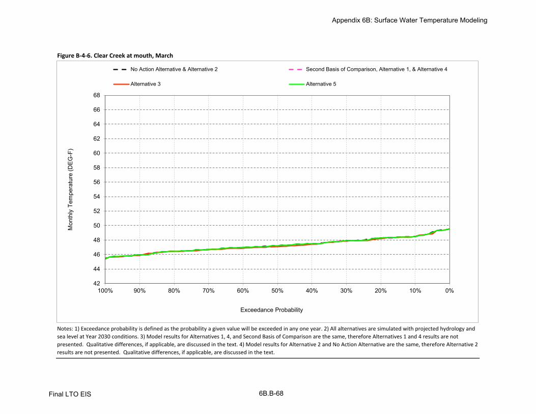
Figure B-4-6. Clear Creek at mouth, March
Notes: 1) Exceedance probability is defined as the probability a given value will be exceeded in any one year. 2) All alternatives are simulated with projected hydrology and
sea level at Year 2030 conditions. 3) Model results for Alternatives 1, 4, and Second Basis of Comparison are the same, therefore Alternatives 1 and 4 results are not
presented. Qualitative differences, if applicable, are discussed in the text. 4) Model results for Alternative 2 and No Action Alternative are the same, therefore Alternative 2
results are not presented. Qualitative differences, if applicable, are discussed in the text.
42
44
46
48
50
52
54
56
58
60
62
64
66
68
0%10%20%30%40%50%60%70%80%90%100%
Exceedance Probability
No Action Alternative & Alternative 2 Second Basis of Comparison, Alternative 1, & Alternative 4
Alternative 3 Alternative 5
Mon
thly
Tem
pera
ture
(DE
G-F
)
Appendix 6B: Surface Water Temperature Modeling
Final LTO EIS 6B.B-68

Figure B-4-7. Clear Creek at mouth, April
Notes: 1) Exceedance probability is defined as the probability a given value will be exceeded in any one year. 2) All alternatives are simulated with projected hydrology and
sea level at Year 2030 conditions. 3) Model results for Alternatives 1, 4, and Second Basis of Comparison are the same, therefore Alternatives 1 and 4 results are not
presented. Qualitative differences, if applicable, are discussed in the text. 4) Model results for Alternative 2 and No Action Alternative are the same, therefore Alternative 2
results are not presented. Qualitative differences, if applicable, are discussed in the text.
42
44
46
48
50
52
54
56
58
60
62
64
66
68
0%10%20%30%40%50%60%70%80%90%100%
Exceedance Probability
No Action Alternative & Alternative 2 Second Basis of Comparison, Alternative 1, & Alternative 4
Alternative 3 Alternative 5
Mon
thly
Tem
pera
ture
(DE
G-F
)
Appendix 6B: Surface Water Temperature Modeling
Final LTO EIS 6B.B-69

Figure B-4-8. Clear Creek at mouth, May
Notes: 1) Exceedance probability is defined as the probability a given value will be exceeded in any one year. 2) All alternatives are simulated with projected hydrology and
sea level at Year 2030 conditions. 3) Model results for Alternatives 1, 4, and Second Basis of Comparison are the same, therefore Alternatives 1 and 4 results are not
presented. Qualitative differences, if applicable, are discussed in the text. 4) Model results for Alternative 2 and No Action Alternative are the same, therefore Alternative 2
results are not presented. Qualitative differences, if applicable, are discussed in the text.
42
44
46
48
50
52
54
56
58
60
62
64
66
68
0%10%20%30%40%50%60%70%80%90%100%
Exceedance Probability
No Action Alternative & Alternative 2 Second Basis of Comparison, Alternative 1, & Alternative 4
Alternative 3 Alternative 5
Mon
thly
Tem
pera
ture
(DE
G-F
)
Appendix 6B: Surface Water Temperature Modeling
Final LTO EIS 6B.B-70

Figure B-4-9. Clear Creek at mouth, June
Notes: 1) Exceedance probability is defined as the probability a given value will be exceeded in any one year. 2) All alternatives are simulated with projected hydrology and
sea level at Year 2030 conditions. 3) Model results for Alternatives 1, 4, and Second Basis of Comparison are the same, therefore Alternatives 1 and 4 results are not
presented. Qualitative differences, if applicable, are discussed in the text. 4) Model results for Alternative 2 and No Action Alternative are the same, therefore Alternative 2
results are not presented. Qualitative differences, if applicable, are discussed in the text.
42
44
46
48
50
52
54
56
58
60
62
64
66
68
0%10%20%30%40%50%60%70%80%90%100%
Exceedance Probability
No Action Alternative & Alternative 2 Second Basis of Comparison, Alternative 1, & Alternative 4
Alternative 3 Alternative 5
Mon
thly
Tem
pera
ture
(DE
G-F
)
Appendix 6B: Surface Water Temperature Modeling
Final LTO EIS 6B.B-71

Figure B-4-10. Clear Creek at mouth, July
Notes: 1) Exceedance probability is defined as the probability a given value will be exceeded in any one year. 2) All alternatives are simulated with projected hydrology and
sea level at Year 2030 conditions. 3) Model results for Alternatives 1, 4, and Second Basis of Comparison are the same, therefore Alternatives 1 and 4 results are not
presented. Qualitative differences, if applicable, are discussed in the text. 4) Model results for Alternative 2 and No Action Alternative are the same, therefore Alternative 2
results are not presented. Qualitative differences, if applicable, are discussed in the text.
42
44
46
48
50
52
54
56
58
60
62
64
66
68
0%10%20%30%40%50%60%70%80%90%100%
Exceedance Probability
No Action Alternative & Alternative 2 Second Basis of Comparison, Alternative 1, & Alternative 4
Alternative 3 Alternative 5
Mon
thly
Tem
pera
ture
(DE
G-F
)
Appendix 6B: Surface Water Temperature Modeling
Final LTO EIS 6B.B-72

Figure B-4-11. Clear Creek at mouth, August
Notes: 1) Exceedance probability is defined as the probability a given value will be exceeded in any one year. 2) All alternatives are simulated with projected hydrology and
sea level at Year 2030 conditions. 3) Model results for Alternatives 1, 4, and Second Basis of Comparison are the same, therefore Alternatives 1 and 4 results are not
presented. Qualitative differences, if applicable, are discussed in the text. 4) Model results for Alternative 2 and No Action Alternative are the same, therefore Alternative 2
results are not presented. Qualitative differences, if applicable, are discussed in the text.
42
44
46
48
50
52
54
56
58
60
62
64
66
68
0%10%20%30%40%50%60%70%80%90%100%
Exceedance Probability
No Action Alternative & Alternative 2 Second Basis of Comparison, Alternative 1, & Alternative 4
Alternative 3 Alternative 5
Mon
thly
Tem
pera
ture
(DE
G-F
)
Appendix 6B: Surface Water Temperature Modeling
Final LTO EIS 6B.B-73

Figure B-4-12. Clear Creek at mouth, September
Notes: 1) Exceedance probability is defined as the probability a given value will be exceeded in any one year. 2) All alternatives are simulated with projected hydrology and
sea level at Year 2030 conditions. 3) Model results for Alternatives 1, 4, and Second Basis of Comparison are the same, therefore Alternatives 1 and 4 results are not
presented. Qualitative differences, if applicable, are discussed in the text. 4) Model results for Alternative 2 and No Action Alternative are the same, therefore Alternative 2
results are not presented. Qualitative differences, if applicable, are discussed in the text.
42
44
46
48
50
52
54
56
58
60
62
64
66
68
0%10%20%30%40%50%60%70%80%90%100%
Exceedance Probability
No Action Alternative & Alternative 2 Second Basis of Comparison, Alternative 1, & Alternative 4
Alternative 3 Alternative 5
Mon
thly
Tem
pera
ture
(DE
G-F
)
Appendix 6B: Surface Water Temperature Modeling
Final LTO EIS 6B.B-74

Oct Nov Dec Jan Feb Mar Apr May Jun Jul Aug Sep
10% 57 53 49 46 47 48 51 52 57 62 62 5820% 56 52 48 46 46 48 50 52 55 62 61 5730% 55 52 48 46 46 48 50 51 55 61 61 5740% 54 51 47 45 46 47 50 51 55 61 61 5650% 54 51 47 45 46 47 49 51 54 61 60 5660% 53 51 47 45 45 47 49 51 54 60 60 5670% 53 50 46 44 45 47 49 50 53 60 60 5580% 52 50 46 44 45 46 49 50 53 60 60 5590% 52 50 46 44 45 46 48 49 53 60 59 54
Full Simulation Periodb 54 51 47 45 46 47 49 51 55 61 60 56
Wet (32%) 51 49 45 45 45 47 49 51 54 61 60 55Above Normal (16%) 54 51 47 45 45 47 49 51 54 60 60 55Below Normal (13%) 53 50 47 45 45 47 50 50 54 61 60 56
Dry (24%) 55 51 47 45 46 48 50 51 55 61 61 57Critical (15%) 56 53 48 46 47 49 51 52 58 61 61 60
Oct Nov Dec Jan Feb Mar Apr May Jun Jul Aug Sep
10% 57 53 49 47 47 48 51 53 57 62 62 5820% 56 52 48 46 46 48 50 53 55 62 61 5730% 55 52 47 46 46 48 50 52 55 61 61 5740% 54 51 47 45 46 47 50 52 55 61 61 5650% 54 51 47 45 46 47 49 52 54 61 60 5660% 53 51 46 45 45 47 49 52 54 60 60 5670% 53 50 46 44 45 47 49 52 54 60 60 5580% 52 50 46 44 45 46 49 51 53 60 60 5590% 52 50 46 44 44 46 48 51 53 60 59 55
Full Simulation Periodb 54 51 47 45 46 47 49 52 55 61 60 56
Wet (32%) 51 49 45 45 45 47 49 52 54 61 60 55Above Normal (16%) 54 51 47 45 45 47 49 52 54 61 60 55Below Normal (13%) 53 50 47 45 45 47 50 52 54 61 60 56
Dry (24%) 54 51 47 45 46 48 50 52 54 61 61 57Critical (15%) 56 53 48 46 47 49 51 53 58 61 61 60
Oct Nov Dec Jan Feb Mar Apr May Jun Jul Aug Sep
0.1 -0.7 -0.2 0.0 0.1 0.0 0.0 -0.1 0.9 0.0 0.2 -0.1 -0.2
0.2 -0.2 0.0 0.2 0.0 0.0 0.0 0.0 1.2 -0.1 -0.1 -0.1 -0.2
0.3 -0.4 0.0 -0.2 0.0 0.0 0.0 -0.1 1.1 0.0 0.1 0.0 -0.2
0.4 -0.1 -0.1 0.0 0.0 -0.1 -0.1 0.0 1.2 0.0 0.0 0.1 0.0
0.5 -0.2 0.1 0.0 0.0 0.0 -0.1 0.0 1.2 -0.1 0.0 0.2 0.20.6 0.2 0.0 -0.1 0.0 -0.2 -0.1 0.0 1.1 0.0 0.1 0.1 -0.1
0.7 0.1 -0.2 0.0 -0.1 -0.1 0.0 -0.1 1.2 0.1 0.1 -0.1 0.10.8 -0.1 0.1 0.0 0.0 -0.1 0.0 0.0 1.3 -0.1 0.2 0.0 0.10.9 0.1 0.0 -0.2 -0.1 0.0 0.0 0.1 1.4 -0.1 0.0 0.1 0.1
Full Simulation Periodb
-0.1 0.0 0.0 0.0 0.0 0.0 0.0 1.2 0.0 0.1 0.0 0.0
Wet (32%) 0.1 -0.1 0.0 0.0 0.0 0.0 0.0 1.2 0.0 0.1 0.1 0.2Above Normal (16%) -0.1 0.0 0.0 0.0 0.0 0.0 0.1 1.3 0.0 0.0 0.0 -0.1
Below Normal (13%) -0.1 0.0 -0.2 0.0 0.0 -0.1 -0.1 1.3 0.2 0.1 0.1 0.0
Dry (24%) -0.4 0.0 0.0 0.0 0.0 0.0 0.0 1.2 -0.1 0.0 0.0 -0.1
Critical (15%) -0.2 -0.1 -0.1 0.0 -0.1 0.0 -0.1 0.9 0.0 0.1 0.1 -0.1
a Exceedance probability is defined as the probability a given value will be exceeded in any one year.
b Based on the 82-year simulation period.
Probability of Exceedancea
Long Term
Water Year Typesc
c As defined by the Sacramento Valley 40-30-30 Index Water Year Hydrologic Classification (SWRCB D-1641, 1999); projected to Year 2030.
Notes: 1) All alternatives are simulated with projected hydrology and sea level at Year 2030 conditions. 2) Model results for Alternatives 1, 4, and Second Basis of Comparison are the same,
therefore Second Basis of Comparison and Alternative 4 results are not presented. Qualitative differences, if applicable, are discussed in the text. 3) Model results for Alternative 2 and No Action
Alternative are the same, therefore Alternative 2 results are not presented. Qualitative differences, if applicable, are discussed in the text.
Probability of Exceedancea
Long Term
Water Year Typesc
Alternative 1 minus No Action Alternative
Statistic
Monthly Temperature (DEG-F)
Long Term
Water Year Typesc
Alternative 1
Statistic
Monthly Temperature (DEG-F)
Table B-4-1. Clear Creek at mouth, Monthly Temperature
No Action Alternative
Statistic
Monthly Temperature (DEG-F)
Probability of Exceedancea
Appendix 6B: Surface Water Temperature Modeling
Final LTO EIS 6B.B-75

Oct Nov Dec Jan Feb Mar Apr May Jun Jul Aug Sep
10% 57 53 49 46 47 48 51 52 57 62 62 5820% 56 52 48 46 46 48 50 52 55 62 61 5730% 55 52 48 46 46 48 50 51 55 61 61 5740% 54 51 47 45 46 47 50 51 55 61 61 5650% 54 51 47 45 46 47 49 51 54 61 60 5660% 53 51 47 45 45 47 49 51 54 60 60 5670% 53 50 46 44 45 47 49 50 53 60 60 5580% 52 50 46 44 45 46 49 50 53 60 60 5590% 52 50 46 44 45 46 48 49 53 60 59 54
Full Simulation Periodb 54 51 47 45 46 47 49 51 55 61 60 56
Wet (32%) 51 49 45 45 45 47 49 51 54 61 60 55Above Normal (16%) 54 51 47 45 45 47 49 51 54 60 60 55Below Normal (13%) 53 50 47 45 45 47 50 50 54 61 60 56
Dry (24%) 55 51 47 45 46 48 50 51 55 61 61 57Critical (15%) 56 53 48 46 47 49 51 52 58 61 61 60
Oct Nov Dec Jan Feb Mar Apr May Jun Jul Aug Sep
10% 57 53 49 47 47 48 51 53 57 62 62 5820% 56 52 48 46 46 48 50 53 55 62 61 5730% 55 52 47 46 46 48 50 52 55 61 61 5740% 54 51 47 45 46 47 50 52 54 61 61 5650% 54 51 47 45 46 47 49 52 54 61 60 5660% 53 51 46 45 45 47 49 52 54 60 60 5670% 53 50 46 44 45 47 49 51 53 60 60 5580% 52 50 46 44 45 46 49 51 53 60 60 5590% 52 50 46 44 44 46 48 51 53 60 59 55
Full Simulation Periodb 54 51 47 45 46 47 49 52 55 61 60 56
Wet (32%) 51 49 45 45 45 47 49 52 54 61 60 55Above Normal (16%) 54 51 47 45 45 47 49 52 54 61 60 55Below Normal (13%) 53 51 47 45 45 47 50 52 54 61 60 56
Dry (24%) 54 51 47 45 46 48 50 52 54 61 61 57Critical (15%) 56 53 48 46 47 49 51 53 58 61 61 60
Oct Nov Dec Jan Feb Mar Apr May Jun Jul Aug Sep
0.1 -0.8 -0.2 0.0 0.1 0.0 0.0 0.1 0.9 0.0 0.2 -0.1 -0.3
0.2 -0.3 -0.1 0.2 0.0 0.0 0.0 0.0 1.2 -0.1 0.0 -0.2 -0.2
0.3 -0.1 0.0 -0.2 0.0 0.0 0.0 -0.1 1.1 -0.1 -0.1 0.0 -0.1
0.4 -0.1 -0.1 -0.1 0.0 -0.1 -0.1 0.0 1.1 -0.1 0.0 0.0 -0.1
0.5 -0.2 0.1 0.0 0.0 0.0 -0.1 0.0 1.2 0.0 -0.1 0.1 0.10.6 0.2 0.0 -0.1 0.0 -0.2 -0.1 0.0 1.1 -0.1 0.1 0.1 -0.1
0.7 0.2 -0.1 -0.1 -0.1 -0.1 0.0 -0.1 1.1 0.0 0.2 0.0 0.10.8 -0.1 0.1 -0.1 -0.1 0.0 0.0 0.0 1.2 -0.1 0.0 0.1 0.10.9 0.1 0.0 -0.2 0.0 -0.1 0.0 0.0 1.3 -0.1 -0.1 0.1 0.1
Full Simulation Periodb
-0.1 -0.1 -0.1 0.0 0.0 -0.1 0.0 1.1 0.0 0.0 0.0 0.0
Wet (32%) 0.1 0.0 0.0 0.0 0.0 -0.1 0.0 1.2 0.0 0.0 0.0 0.2Above Normal (16%) -0.1 0.0 -0.1 0.0 0.0 0.0 0.0 1.2 0.0 0.0 0.0 0.0
Below Normal (13%) 0.0 0.0 -0.2 0.0 -0.1 -0.1 -0.1 1.3 0.1 0.1 0.1 -0.1
Dry (24%) -0.4 0.0 0.0 0.0 0.0 0.0 -0.1 1.1 -0.1 0.0 -0.1 -0.1
Critical (15%) -0.4 -0.3 -0.2 -0.1 -0.1 -0.1 -0.1 0.8 -0.1 0.0 0.1 -0.2
a Exceedance probability is defined as the probability a given value will be exceeded in any one year.
b Based on the 82-year simulation period.
Probability of Exceedancea
Long Term
Water Year Typesc
c As defined by the Sacramento Valley 40-30-30 Index Water Year Hydrologic Classification (SWRCB D-1641, 1999); projected to Year 2030.
Notes: 1) All alternatives are simulated with projected hydrology and sea level at Year 2030 conditions. 2) Model results for Alternatives 1, 4, and Second Basis of Comparison are the same,
therefore Alternative 1 and 4 results are not presented. Qualitative differences, if applicable, are discussed in the text. 3) Model results for Alternative 2 and No Action Alternative are the same,
therefore Alternative 2 results are not presented. Qualitative differences, if applicable, are discussed in the text.
Probability of Exceedancea
Long Term
Water Year Typesc
Alternative 3 minus No Action Alternative
Statistic
Monthly Temperature (DEG-F)
Long Term
Water Year Typesc
Alternative 3
Statistic
Monthly Temperature (DEG-F)
Table B-4-2. Clear Creek at mouth, Monthly Temperature
No Action Alternative
Statistic
Monthly Temperature (DEG-F)
Probability of Exceedancea
Appendix 6B: Surface Water Temperature Modeling
Final LTO EIS 6B.B-76

Oct Nov Dec Jan Feb Mar Apr May Jun Jul Aug Sep
10% 57 53 49 46 47 48 51 52 57 62 62 5820% 56 52 48 46 46 48 50 52 55 62 61 5730% 55 52 48 46 46 48 50 51 55 61 61 5740% 54 51 47 45 46 47 50 51 55 61 61 5650% 54 51 47 45 46 47 49 51 54 61 60 5660% 53 51 47 45 45 47 49 51 54 60 60 5670% 53 50 46 44 45 47 49 50 53 60 60 5580% 52 50 46 44 45 46 49 50 53 60 60 5590% 52 50 46 44 45 46 48 49 53 60 59 54
Full Simulation Periodb 54 51 47 45 46 47 49 51 55 61 60 56
Wet (32%) 51 49 45 45 45 47 49 51 54 61 60 55Above Normal (16%) 54 51 47 45 45 47 49 51 54 60 60 55Below Normal (13%) 53 50 47 45 45 47 50 50 54 61 60 56
Dry (24%) 55 51 47 45 46 48 50 51 55 61 61 57Critical (15%) 56 53 48 46 47 49 51 52 58 61 61 60
Oct Nov Dec Jan Feb Mar Apr May Jun Jul Aug Sep
10% 57 53 49 46 47 48 51 53 57 62 62 5820% 56 52 48 46 46 48 50 52 56 62 61 5730% 55 52 48 46 46 48 50 51 55 61 61 5740% 54 51 47 45 46 47 50 51 55 61 61 5750% 54 51 47 45 46 47 49 51 54 61 60 5660% 53 51 47 45 45 47 49 51 54 60 60 5670% 53 50 46 44 45 47 49 50 53 60 60 5580% 52 50 46 44 45 46 49 50 53 60 60 5590% 52 50 46 44 45 46 48 49 53 60 59 54
Full Simulation Periodb 54 51 47 45 46 47 49 51 55 61 60 56
Wet (32%) 51 49 45 45 45 47 49 51 54 61 60 55Above Normal (16%) 55 51 47 45 45 47 49 50 54 60 60 55Below Normal (13%) 53 50 47 45 45 47 50 51 54 61 60 56
Dry (24%) 55 51 47 45 46 48 50 51 54 61 61 57Critical (15%) 56 53 48 46 47 49 51 53 58 61 61 59
Oct Nov Dec Jan Feb Mar Apr May Jun Jul Aug Sep
0.1 0.0 0.1 0.0 0.0 0.0 0.0 0.1 0.1 0.0 0.1 0.0 -0.1
0.2 0.0 0.0 0.0 0.0 0.0 0.0 0.0 0.1 0.0 0.0 -0.1 0.00.3 0.0 0.0 0.1 0.0 0.0 0.0 0.0 0.0 0.0 0.1 0.0 0.0
0.4 -0.1 0.0 0.0 0.0 0.0 0.0 0.0 0.0 0.0 0.1 0.0 0.10.5 0.0 0.0 0.0 0.0 0.0 0.0 0.0 0.0 0.0 0.0 0.0 0.00.6 0.0 -0.1 0.0 0.0 0.0 0.0 0.0 0.0 0.0 0.0 0.0 -0.2
0.7 0.0 0.0 0.0 0.0 0.0 0.0 0.0 0.0 0.0 0.0 -0.1 0.00.8 0.0 0.0 0.0 0.0 0.0 0.0 0.0 0.1 0.0 0.0 0.0 0.0
0.9 0.0 0.0 0.0 0.0 0.0 0.0 0.0 0.0 0.0 0.0 0.1 0.0
Full Simulation Periodb
-0.1 0.0 0.0 0.0 0.0 0.0 0.0 0.1 0.1 0.0 0.0 0.0
Wet (32%) 0.0 0.0 0.0 0.0 0.0 0.0 0.0 0.0 0.0 0.0 0.0 0.0
Above Normal (16%) 0.1 0.1 0.0 0.0 0.0 0.0 0.0 0.0 0.0 0.0 0.0 0.0
Below Normal (13%) 0.0 0.0 0.0 0.0 0.0 0.0 0.0 0.2 0.1 0.0 0.1 0.1Dry (24%) -0.3 0.0 0.0 0.0 0.0 0.0 0.0 0.0 0.0 0.0 0.0 0.0
Critical (15%) 0.0 0.0 0.0 0.0 0.0 0.0 0.0 0.3 0.3 0.2 -0.2 -0.2
a Exceedance probability is defined as the probability a given value will be exceeded in any one year.
b Based on the 82-year simulation period.
Probability of Exceedancea
Long Term
Water Year Typesc
c As defined by the Sacramento Valley 40-30-30 Index Water Year Hydrologic Classification (SWRCB D-1641, 1999); projected to Year 2030.
Notes: 1) All alternatives are simulated with projected hydrology and sea level at Year 2030 conditions. 2) Model results for Alternatives 1, 4, and Second Basis of Comparison are the same,
therefore Alternative 1 and 4 results are not presented. Qualitative differences, if applicable, are discussed in the text. 3) Model results for Alternative 2 and No Action Alternative are the same,
therefore Alternative 2 results are not presented. Qualitative differences, if applicable, are discussed in the text.
Probability of Exceedancea
Long Term
Water Year Typesc
Alternative 5 minus No Action Alternative
Statistic
Monthly Temperature (DEG-F)
Long Term
Water Year Typesc
Alternative 5
Statistic
Monthly Temperature (DEG-F)
Table B-4-3. Clear Creek at mouth, Monthly Temperature
No Action Alternative
Statistic
Monthly Temperature (DEG-F)
Probability of Exceedancea
Appendix 6B: Surface Water Temperature Modeling
Final LTO EIS 6B.B-77

Oct Nov Dec Jan Feb Mar Apr May Jun Jul Aug Sep
10% 57 53 49 47 47 48 51 53 57 62 62 5820% 56 52 48 46 46 48 50 53 55 62 61 5730% 55 52 47 46 46 48 50 52 55 61 61 5740% 54 51 47 45 46 47 50 52 55 61 61 5650% 54 51 47 45 46 47 49 52 54 61 60 5660% 53 51 46 45 45 47 49 52 54 60 60 5670% 53 50 46 44 45 47 49 52 54 60 60 5580% 52 50 46 44 45 46 49 51 53 60 60 5590% 52 50 46 44 44 46 48 51 53 60 59 55
Full Simulation Periodb 54 51 47 45 46 47 49 52 55 61 60 56
Wet (32%) 51 49 45 45 45 47 49 52 54 61 60 55Above Normal (16%) 54 51 47 45 45 47 49 52 54 61 60 55Below Normal (13%) 53 50 47 45 45 47 50 52 54 61 60 56
Dry (24%) 54 51 47 45 46 48 50 52 54 61 61 57Critical (15%) 56 53 48 46 47 49 51 53 58 61 61 60
Oct Nov Dec Jan Feb Mar Apr May Jun Jul Aug Sep
10% 57 53 49 46 47 48 51 52 57 62 62 5820% 56 52 48 46 46 48 50 52 55 62 61 5730% 55 52 48 46 46 48 50 51 55 61 61 5740% 54 51 47 45 46 47 50 51 55 61 61 5650% 54 51 47 45 46 47 49 51 54 61 60 5660% 53 51 47 45 45 47 49 51 54 60 60 5670% 53 50 46 44 45 47 49 50 53 60 60 5580% 52 50 46 44 45 46 49 50 53 60 60 5590% 52 50 46 44 45 46 48 49 53 60 59 54
Full Simulation Periodb 54 51 47 45 46 47 49 51 55 61 60 56
Wet (32%) 51 49 45 45 45 47 49 51 54 61 60 55Above Normal (16%) 54 51 47 45 45 47 49 51 54 60 60 55Below Normal (13%) 53 50 47 45 45 47 50 50 54 61 60 56
Dry (24%) 55 51 47 45 46 48 50 51 55 61 61 57Critical (15%) 56 53 48 46 47 49 51 52 58 61 61 60
Oct Nov Dec Jan Feb Mar Apr May Jun Jul Aug Sep
0.1 0.7 0.2 0.0 -0.1 0.0 0.0 0.1 -0.9 0.0 -0.2 0.1 0.20.2 0.2 0.0 -0.2 0.0 0.0 0.0 0.0 -1.2 0.1 0.1 0.1 0.20.3 0.4 0.0 0.2 0.0 0.0 0.0 0.1 -1.1 0.0 -0.1 0.0 0.20.4 0.1 0.1 0.0 0.0 0.1 0.1 0.0 -1.2 0.0 0.0 -0.1 0.00.5 0.2 -0.1 0.0 0.0 0.0 0.1 0.0 -1.2 0.1 0.0 -0.2 -0.2
0.6 -0.2 0.0 0.1 0.0 0.2 0.1 0.0 -1.1 0.0 -0.1 -0.1 0.10.7 -0.1 0.2 0.0 0.1 0.1 0.0 0.1 -1.2 -0.1 -0.1 0.1 -0.1
0.8 0.1 -0.1 0.0 0.0 0.1 0.0 0.0 -1.3 0.1 -0.2 0.0 -0.1
0.9 -0.1 0.0 0.2 0.1 0.0 0.0 -0.1 -1.4 0.1 0.0 -0.1 -0.1
Full Simulation Periodb 0.1 0.0 0.0 0.0 0.0 0.0 0.0 -1.2 0.0 -0.1 0.0 0.0
Wet (32%) -0.1 0.1 0.0 0.0 0.0 0.0 0.0 -1.2 0.0 -0.1 -0.1 -0.2
Above Normal (16%) 0.1 0.0 0.0 0.0 0.0 0.0 -0.1 -1.3 0.0 0.0 0.0 0.1Below Normal (13%) 0.1 0.0 0.2 0.0 0.0 0.1 0.1 -1.3 -0.2 -0.1 -0.1 0.0
Dry (24%) 0.4 0.0 0.0 0.0 0.0 0.0 0.0 -1.2 0.1 0.0 0.0 0.1Critical (15%) 0.2 0.1 0.1 0.0 0.1 0.0 0.1 -0.9 0.0 -0.1 -0.1 0.1
a Exceedance probability is defined as the probability a given value will be exceeded in any one year.
b Based on the 82-year simulation period.
Probability of Exceedancea
Long Term
Water Year Typesc
c As defined by the Sacramento Valley 40-30-30 Index Water Year Hydrologic Classification (SWRCB D-1641, 1999); projected to Year 2030.
Notes: 1) All alternatives are simulated with projected hydrology and sea level at Year 2030 conditions. 2) Model results for Alternatives 1, 4, and Second Basis of Comparison are the same,
therefore Alternative 1 and 4 results are not presented. Qualitative differences, if applicable, are discussed in the text. 3) Model results for Alternative 2 and No Action Alternative are the same,
therefore Alternative 2 results are not presented. Qualitative differences, if applicable, are discussed in the text.
Probability of Exceedancea
Long Term
Water Year Typesc
No Action Alternative minus Second Basis of Comparison
Statistic
Monthly Temperature (DEG-F)
Long Term
Water Year Typesc
No Action Alternative
Statistic
Monthly Temperature (DEG-F)
Table B-4-4. Clear Creek at mouth, Monthly Temperature
Second Basis of Comparison
Statistic
Monthly Temperature (DEG-F)
Probability of Exceedancea
Appendix 6B: Surface Water Temperature Modeling
Final LTO EIS 6B.B-78

Oct Nov Dec Jan Feb Mar Apr May Jun Jul Aug Sep
10% 57 53 49 47 47 48 51 53 57 62 62 5820% 56 52 48 46 46 48 50 53 55 62 61 5730% 55 52 47 46 46 48 50 52 55 61 61 5740% 54 51 47 45 46 47 50 52 55 61 61 5650% 54 51 47 45 46 47 49 52 54 61 60 5660% 53 51 46 45 45 47 49 52 54 60 60 5670% 53 50 46 44 45 47 49 52 54 60 60 5580% 52 50 46 44 45 46 49 51 53 60 60 5590% 52 50 46 44 44 46 48 51 53 60 59 55
Full Simulation Periodb 54 51 47 45 46 47 49 52 55 61 60 56
Wet (32%) 51 49 45 45 45 47 49 52 54 61 60 55Above Normal (16%) 54 51 47 45 45 47 49 52 54 61 60 55Below Normal (13%) 53 50 47 45 45 47 50 52 54 61 60 56
Dry (24%) 54 51 47 45 46 48 50 52 54 61 61 57Critical (15%) 56 53 48 46 47 49 51 53 58 61 61 60
Oct Nov Dec Jan Feb Mar Apr May Jun Jul Aug Sep
10% 57 53 49 47 47 48 51 53 57 62 62 5820% 56 52 48 46 46 48 50 53 55 62 61 5730% 55 52 47 46 46 48 50 52 55 61 61 5740% 54 51 47 45 46 47 50 52 54 61 61 5650% 54 51 47 45 46 47 49 52 54 61 60 5660% 53 51 46 45 45 47 49 52 54 60 60 5670% 53 50 46 44 45 47 49 51 53 60 60 5580% 52 50 46 44 45 46 49 51 53 60 60 5590% 52 50 46 44 44 46 48 51 53 60 59 55
Full Simulation Periodb 54 51 47 45 46 47 49 52 55 61 60 56
Wet (32%) 51 49 45 45 45 47 49 52 54 61 60 55Above Normal (16%) 54 51 47 45 45 47 49 52 54 61 60 55Below Normal (13%) 53 51 47 45 45 47 50 52 54 61 60 56
Dry (24%) 54 51 47 45 46 48 50 52 54 61 61 57Critical (15%) 56 53 48 46 47 49 51 53 58 61 61 60
Oct Nov Dec Jan Feb Mar Apr May Jun Jul Aug Sep
0.1 0.0 0.0 0.0 0.0 0.0 0.0 0.2 -0.1 0.0 0.0 0.0 -0.1
0.2 0.0 -0.1 0.0 0.0 0.0 0.0 0.0 0.0 0.0 0.0 -0.1 0.0
0.3 0.2 0.0 0.0 0.0 0.0 0.0 0.0 0.0 -0.1 -0.2 0.0 0.10.4 0.1 0.0 -0.1 0.0 0.0 0.0 0.0 -0.1 -0.1 0.0 -0.1 0.0
0.5 0.0 0.0 0.0 0.0 0.0 0.0 0.0 -0.1 0.1 0.0 0.0 0.0
0.6 -0.1 0.0 0.0 0.0 0.0 0.0 0.0 0.0 -0.1 0.0 -0.1 0.0
0.7 0.1 0.1 0.0 0.0 0.0 0.0 0.0 -0.1 -0.1 0.0 0.0 0.0
0.8 0.0 0.0 0.0 -0.1 0.0 0.0 0.0 -0.1 -0.1 -0.2 0.1 0.00.9 0.0 0.0 -0.1 0.2 0.0 0.0 -0.1 -0.1 0.0 -0.1 0.0 -0.1
Full Simulation Periodb
0.0 0.0 0.0 0.0 0.0 0.0 0.0 0.0 0.0 0.0 0.0 0.0
Wet (32%) 0.0 0.0 0.0 0.0 0.0 0.0 0.0 0.0 0.0 0.0 0.0 0.0Above Normal (16%) 0.0 0.0 0.0 0.0 0.0 0.0 0.0 -0.1 0.0 0.0 0.0 0.0Below Normal (13%) 0.0 0.0 0.0 0.0 0.0 0.0 0.0 0.0 -0.1 0.0 0.0 0.0
Dry (24%) 0.0 0.0 0.0 0.0 0.0 0.0 0.0 -0.1 -0.1 -0.1 -0.1 0.0
Critical (15%) -0.1 -0.2 -0.1 0.0 0.0 0.0 0.0 0.0 -0.1 -0.1 0.0 0.0
a Exceedance probability is defined as the probability a given value will be exceeded in any one year.
b Based on the 82-year simulation period.
Probability of Exceedancea
Long Term
Water Year Typesc
c As defined by the Sacramento Valley 40-30-30 Index Water Year Hydrologic Classification (SWRCB D-1641, 1999); projected to Year 2030.
Notes: 1) All alternatives are simulated with projected hydrology and sea level at Year 2030 conditions. 2) Model results for Alternatives 1, 4, and Second Basis of Comparison are the same,
therefore Alternative 1 and 4 results are not presented. Qualitative differences, if applicable, are discussed in the text. 3) Model results for Alternative 2 and No Action Alternative are the same,
therefore Alternative 2 results are not presented. Qualitative differences, if applicable, are discussed in the text.
Probability of Exceedancea
Long Term
Water Year Typesc
Alternative 3 minus Second Basis of Comparison
Statistic
Monthly Temperature (DEG-F)
Long Term
Water Year Typesc
Alternative 3
Statistic
Monthly Temperature (DEG-F)
Table B-4-5. Clear Creek at mouth, Monthly Temperature
Second Basis of Comparison
Statistic
Monthly Temperature (DEG-F)
Probability of Exceedancea
Appendix 6B: Surface Water Temperature Modeling
Final LTO EIS 6B.B-79

Oct Nov Dec Jan Feb Mar Apr May Jun Jul Aug Sep
10% 57 53 49 47 47 48 51 53 57 62 62 5820% 56 52 48 46 46 48 50 53 55 62 61 5730% 55 52 47 46 46 48 50 52 55 61 61 5740% 54 51 47 45 46 47 50 52 55 61 61 5650% 54 51 47 45 46 47 49 52 54 61 60 5660% 53 51 46 45 45 47 49 52 54 60 60 5670% 53 50 46 44 45 47 49 52 54 60 60 5580% 52 50 46 44 45 46 49 51 53 60 60 5590% 52 50 46 44 44 46 48 51 53 60 59 55
Full Simulation Periodb 54 51 47 45 46 47 49 52 55 61 60 56
Wet (32%) 51 49 45 45 45 47 49 52 54 61 60 55Above Normal (16%) 54 51 47 45 45 47 49 52 54 61 60 55Below Normal (13%) 53 50 47 45 45 47 50 52 54 61 60 56
Dry (24%) 54 51 47 45 46 48 50 52 54 61 61 57Critical (15%) 56 53 48 46 47 49 51 53 58 61 61 60
Oct Nov Dec Jan Feb Mar Apr May Jun Jul Aug Sep
10% 57 53 49 46 47 48 51 53 57 62 62 5820% 56 52 48 46 46 48 50 52 56 62 61 5730% 55 52 48 46 46 48 50 51 55 61 61 5740% 54 51 47 45 46 47 50 51 55 61 61 5750% 54 51 47 45 46 47 49 51 54 61 60 5660% 53 51 47 45 45 47 49 51 54 60 60 5670% 53 50 46 44 45 47 49 50 53 60 60 5580% 52 50 46 44 45 46 49 50 53 60 60 5590% 52 50 46 44 45 46 48 49 53 60 59 54
Full Simulation Periodb 54 51 47 45 46 47 49 51 55 61 60 56
Wet (32%) 51 49 45 45 45 47 49 51 54 61 60 55Above Normal (16%) 55 51 47 45 45 47 49 50 54 60 60 55Below Normal (13%) 53 50 47 45 45 47 50 51 54 61 60 56
Dry (24%) 55 51 47 45 46 48 50 51 54 61 61 57Critical (15%) 56 53 48 46 47 49 51 53 58 61 61 59
Oct Nov Dec Jan Feb Mar Apr May Jun Jul Aug Sep
0.1 0.7 0.2 -0.1 -0.1 0.0 0.0 0.2 -0.9 0.0 -0.1 0.1 0.10.2 0.2 0.0 -0.2 0.0 0.0 0.0 0.0 -1.1 0.1 0.1 0.0 0.20.3 0.4 0.0 0.3 0.0 0.0 0.0 0.1 -1.1 0.0 0.0 -0.1 0.20.4 0.0 0.1 0.0 0.0 0.1 0.1 0.0 -1.2 0.0 0.0 -0.1 0.10.5 0.1 -0.1 0.0 0.0 0.0 0.1 0.0 -1.2 0.1 0.0 -0.2 -0.1
0.6 -0.3 0.0 0.0 0.0 0.1 0.1 0.0 -1.1 0.0 -0.1 -0.2 -0.1
0.7 -0.2 0.1 0.0 0.1 0.1 0.0 0.1 -1.2 0.0 -0.1 0.0 -0.1
0.8 0.1 0.0 0.0 0.0 0.1 0.0 0.0 -1.2 0.0 -0.1 0.0 -0.1
0.9 -0.1 0.1 0.1 0.2 0.0 0.0 -0.1 -1.4 0.1 0.0 0.0 -0.1
Full Simulation Periodb 0.1 0.0 0.0 0.0 0.0 0.0 0.0 -1.1 0.1 0.0 -0.1 0.0
Wet (32%) -0.1 0.1 0.0 0.0 0.0 0.0 0.0 -1.1 0.0 0.0 0.0 -0.2
Above Normal (16%) 0.2 0.1 0.0 0.0 0.0 0.0 -0.1 -1.3 0.0 0.0 0.0 0.0Below Normal (13%) 0.0 0.0 0.2 0.0 0.0 0.1 0.1 -1.1 -0.1 -0.1 0.0 0.1
Dry (24%) 0.1 0.0 0.0 0.0 0.0 0.0 0.0 -1.2 0.1 0.0 0.0 0.1Critical (15%) 0.2 0.1 0.1 0.0 0.1 0.0 0.1 -0.6 0.3 0.1 -0.2 -0.1
a Exceedance probability is defined as the probability a given value will be exceeded in any one year.
b Based on the 82-year simulation period.
Probability of Exceedancea
Long Term
Water Year Typesc
c As defined by the Sacramento Valley 40-30-30 Index Water Year Hydrologic Classification (SWRCB D-1641, 1999); projected to Year 2030.
Notes: 1) All alternatives are simulated with projected hydrology and sea level at Year 2030 conditions. 2) Model results for Alternatives 1, 4, and Second Basis of Comparison are the same,
therefore Alternative 1 and 4 results are not presented. Qualitative differences, if applicable, are discussed in the text. 3) Model results for Alternative 2 and No Action Alternative are the same,
therefore Alternative 2 results are not presented. Qualitative differences, if applicable, are discussed in the text.
Probability of Exceedancea
Long Term
Water Year Typesc
Alternative 5 minus Second Basis of Comparison
Statistic
Monthly Temperature (DEG-F)
Long Term
Water Year Typesc
Alternative 5
Statistic
Monthly Temperature (DEG-F)
Table B-4-6. Clear Creek at mouth, Monthly Temperature
Second Basis of Comparison
Statistic
Monthly Temperature (DEG-F)
Probability of Exceedancea
Appendix 6B: Surface Water Temperature Modeling
Final LTO EIS 6B.B-80

B.5. Sacramento River below Keswick Temperature
Appendix 6B: Surface Water Temperature Modeling
Final LTO EIS 6B.B-81

Figure B-5-1. Sacramento River below Keswick, October
Notes: 1) Exceedance probability is defined as the probability a given value will be exceeded in any one year. 2) All alternatives are simulated with projected hydrology and
sea level at Year 2030 conditions. 3) Model results for Alternatives 1, 4, and Second Basis of Comparison are the same, therefore Alternatives 1 and 4 results are not
presented. Qualitative differences, if applicable, are discussed in the text. 4) Model results for Alternative 2 and No Action Alternative are the same, therefore Alternative 2
results are not presented. Qualitative differences, if applicable, are discussed in the text.
42
44
46
48
50
52
54
56
58
60
62
64
66
68
0%10%20%30%40%50%60%70%80%90%100%
Exceedance Probability
No Action Alternative & Alternative 2 Second Basis of Comparison, Alternative 1, & Alternative 4
Alternative 3 Alternative 5
Mon
thly
Tem
pera
ture
(DE
G-F
)
Appendix 6B: Surface Water Temperature Modeling
Final LTO EIS 6B.B-82

Figure B-5-2. Sacramento River below Keswick, November
Notes: 1) Exceedance probability is defined as the probability a given value will be exceeded in any one year. 2) All alternatives are simulated with projected hydrology and
sea level at Year 2030 conditions. 3) Model results for Alternatives 1, 4, and Second Basis of Comparison are the same, therefore Alternatives 1 and 4 results are not
presented. Qualitative differences, if applicable, are discussed in the text. 4) Model results for Alternative 2 and No Action Alternative are the same, therefore Alternative 2
results are not presented. Qualitative differences, if applicable, are discussed in the text.
42
44
46
48
50
52
54
56
58
60
62
64
66
68
0%10%20%30%40%50%60%70%80%90%100%
Exceedance Probability
No Action Alternative & Alternative 2 Second Basis of Comparison, Alternative 1, & Alternative 4
Alternative 3 Alternative 5
Mon
thly
Tem
pera
ture
(DE
G-F
)
Appendix 6B: Surface Water Temperature Modeling
Final LTO EIS 6B.B-83

Figure B-5-3. Sacramento River below Keswick, December
Notes: 1) Exceedance probability is defined as the probability a given value will be exceeded in any one year. 2) All alternatives are simulated with projected hydrology and
sea level at Year 2030 conditions. 3) Model results for Alternatives 1, 4, and Second Basis of Comparison are the same, therefore Alternatives 1 and 4 results are not
presented. Qualitative differences, if applicable, are discussed in the text. 4) Model results for Alternative 2 and No Action Alternative are the same, therefore Alternative 2
results are not presented. Qualitative differences, if applicable, are discussed in the text.
42
44
46
48
50
52
54
56
58
60
62
64
66
68
0%10%20%30%40%50%60%70%80%90%100%
Exceedance Probability
No Action Alternative & Alternative 2 Second Basis of Comparison, Alternative 1, & Alternative 4
Alternative 3 Alternative 5
Mon
thly
Tem
pera
ture
(DE
G-F
)
Appendix 6B: Surface Water Temperature Modeling
Final LTO EIS 6B.B-84

Figure B-5-4. Sacramento River below Keswick, January
Notes: 1) Exceedance probability is defined as the probability a given value will be exceeded in any one year. 2) All alternatives are simulated with projected hydrology and
sea level at Year 2030 conditions. 3) Model results for Alternatives 1, 4, and Second Basis of Comparison are the same, therefore Alternatives 1 and 4 results are not
presented. Qualitative differences, if applicable, are discussed in the text. 4) Model results for Alternative 2 and No Action Alternative are the same, therefore Alternative 2
results are not presented. Qualitative differences, if applicable, are discussed in the text.
42
44
46
48
50
52
54
56
58
60
62
64
66
68
0%10%20%30%40%50%60%70%80%90%100%
Exceedance Probability
No Action Alternative & Alternative 2 Second Basis of Comparison, Alternative 1, & Alternative 4
Alternative 3 Alternative 5
Mon
thly
Tem
pera
ture
(DE
G-F
)
Appendix 6B: Surface Water Temperature Modeling
Final LTO EIS 6B.B-85

Figure B-5-5. Sacramento River below Keswick, February
Notes: 1) Exceedance probability is defined as the probability a given value will be exceeded in any one year. 2) All alternatives are simulated with projected hydrology and
sea level at Year 2030 conditions. 3) Model results for Alternatives 1, 4, and Second Basis of Comparison are the same, therefore Alternatives 1 and 4 results are not
presented. Qualitative differences, if applicable, are discussed in the text. 4) Model results for Alternative 2 and No Action Alternative are the same, therefore Alternative 2
results are not presented. Qualitative differences, if applicable, are discussed in the text.
42
44
46
48
50
52
54
56
58
60
62
64
66
68
0%10%20%30%40%50%60%70%80%90%100%
Exceedance Probability
No Action Alternative & Alternative 2 Second Basis of Comparison, Alternative 1, & Alternative 4
Alternative 3 Alternative 5
Mon
thly
Tem
pera
ture
(DE
G-F
)
Appendix 6B: Surface Water Temperature Modeling
Final LTO EIS 6B.B-86

Figure B-5-6. Sacramento River below Keswick, March
Notes: 1) Exceedance probability is defined as the probability a given value will be exceeded in any one year. 2) All alternatives are simulated with projected hydrology and
sea level at Year 2030 conditions. 3) Model results for Alternatives 1, 4, and Second Basis of Comparison are the same, therefore Alternatives 1 and 4 results are not
presented. Qualitative differences, if applicable, are discussed in the text. 4) Model results for Alternative 2 and No Action Alternative are the same, therefore Alternative 2
results are not presented. Qualitative differences, if applicable, are discussed in the text.
42
44
46
48
50
52
54
56
58
60
62
64
66
68
0%10%20%30%40%50%60%70%80%90%100%
Exceedance Probability
No Action Alternative & Alternative 2 Second Basis of Comparison, Alternative 1, & Alternative 4
Alternative 3 Alternative 5
Mon
thly
Tem
pera
ture
(DE
G-F
)
Appendix 6B: Surface Water Temperature Modeling
Final LTO EIS 6B.B-87

Figure B-5-7. Sacramento River below Keswick, April
Notes: 1) Exceedance probability is defined as the probability a given value will be exceeded in any one year. 2) All alternatives are simulated with projected hydrology and
sea level at Year 2030 conditions. 3) Model results for Alternatives 1, 4, and Second Basis of Comparison are the same, therefore Alternatives 1 and 4 results are not
presented. Qualitative differences, if applicable, are discussed in the text. 4) Model results for Alternative 2 and No Action Alternative are the same, therefore Alternative 2
results are not presented. Qualitative differences, if applicable, are discussed in the text.
42
44
46
48
50
52
54
56
58
60
62
64
66
68
0%10%20%30%40%50%60%70%80%90%100%
Exceedance Probability
No Action Alternative & Alternative 2 Second Basis of Comparison, Alternative 1, & Alternative 4
Alternative 3 Alternative 5
Mon
thly
Tem
pera
ture
(DE
G-F
)
Appendix 6B: Surface Water Temperature Modeling
Final LTO EIS 6B.B-88

Figure B-5-8. Sacramento River below Keswick, May
Notes: 1) Exceedance probability is defined as the probability a given value will be exceeded in any one year. 2) All alternatives are simulated with projected hydrology and
sea level at Year 2030 conditions. 3) Model results for Alternatives 1, 4, and Second Basis of Comparison are the same, therefore Alternatives 1 and 4 results are not
presented. Qualitative differences, if applicable, are discussed in the text. 4) Model results for Alternative 2 and No Action Alternative are the same, therefore Alternative 2
results are not presented. Qualitative differences, if applicable, are discussed in the text.
42
44
46
48
50
52
54
56
58
60
62
64
66
68
0%10%20%30%40%50%60%70%80%90%100%
Exceedance Probability
No Action Alternative & Alternative 2 Second Basis of Comparison, Alternative 1, & Alternative 4
Alternative 3 Alternative 5
Mon
thly
Tem
pera
ture
(DE
G-F
)
Appendix 6B: Surface Water Temperature Modeling
Final LTO EIS 6B.B-89

Figure B-5-9. Sacramento River below Keswick, June
Notes: 1) Exceedance probability is defined as the probability a given value will be exceeded in any one year. 2) All alternatives are simulated with projected hydrology and
sea level at Year 2030 conditions. 3) Model results for Alternatives 1, 4, and Second Basis of Comparison are the same, therefore Alternatives 1 and 4 results are not
presented. Qualitative differences, if applicable, are discussed in the text. 4) Model results for Alternative 2 and No Action Alternative are the same, therefore Alternative 2
results are not presented. Qualitative differences, if applicable, are discussed in the text.
42
44
46
48
50
52
54
56
58
60
62
64
66
68
0%10%20%30%40%50%60%70%80%90%100%
Exceedance Probability
No Action Alternative & Alternative 2 Second Basis of Comparison, Alternative 1, & Alternative 4
Alternative 3 Alternative 5
Mon
thly
Tem
pera
ture
(DE
G-F
)
Appendix 6B: Surface Water Temperature Modeling
Final LTO EIS 6B.B-90

Figure B-5-10. Sacramento River below Keswick, July
Notes: 1) Exceedance probability is defined as the probability a given value will be exceeded in any one year. 2) All alternatives are simulated with projected hydrology and
sea level at Year 2030 conditions. 3) Model results for Alternatives 1, 4, and Second Basis of Comparison are the same, therefore Alternatives 1 and 4 results are not
presented. Qualitative differences, if applicable, are discussed in the text. 4) Model results for Alternative 2 and No Action Alternative are the same, therefore Alternative 2
results are not presented. Qualitative differences, if applicable, are discussed in the text.
42
44
46
48
50
52
54
56
58
60
62
64
66
68
0%10%20%30%40%50%60%70%80%90%100%
Exceedance Probability
No Action Alternative & Alternative 2 Second Basis of Comparison, Alternative 1, & Alternative 4
Alternative 3 Alternative 5
Mon
thly
Tem
pera
ture
(DE
G-F
)
Appendix 6B: Surface Water Temperature Modeling
Final LTO EIS 6B.B-91

Figure B-5-11. Sacramento River below Keswick, August
Notes: 1) Exceedance probability is defined as the probability a given value will be exceeded in any one year. 2) All alternatives are simulated with projected hydrology and
sea level at Year 2030 conditions. 3) Model results for Alternatives 1, 4, and Second Basis of Comparison are the same, therefore Alternatives 1 and 4 results are not
presented. Qualitative differences, if applicable, are discussed in the text. 4) Model results for Alternative 2 and No Action Alternative are the same, therefore Alternative 2
results are not presented. Qualitative differences, if applicable, are discussed in the text.
42
44
46
48
50
52
54
56
58
60
62
64
66
68
0%10%20%30%40%50%60%70%80%90%100%
Exceedance Probability
No Action Alternative & Alternative 2 Second Basis of Comparison, Alternative 1, & Alternative 4
Alternative 3 Alternative 5
Mon
thly
Tem
pera
ture
(DE
G-F
)
Appendix 6B: Surface Water Temperature Modeling
Final LTO EIS 6B.B-92

Figure B-5-12. Sacramento River below Keswick, September
Notes: 1) Exceedance probability is defined as the probability a given value will be exceeded in any one year. 2) All alternatives are simulated with projected hydrology and
sea level at Year 2030 conditions. 3) Model results for Alternatives 1, 4, and Second Basis of Comparison are the same, therefore Alternatives 1 and 4 results are not
presented. Qualitative differences, if applicable, are discussed in the text. 4) Model results for Alternative 2 and No Action Alternative are the same, therefore Alternative 2
results are not presented. Qualitative differences, if applicable, are discussed in the text.
42
44
46
48
50
52
54
56
58
60
62
64
66
68
0%10%20%30%40%50%60%70%80%90%100%
Exceedance Probability
No Action Alternative & Alternative 2 Second Basis of Comparison, Alternative 1, & Alternative 4
Alternative 3 Alternative 5
Mon
thly
Tem
pera
ture
(DE
G-F
)
Appendix 6B: Surface Water Temperature Modeling
Final LTO EIS 6B.B-93

Oct Nov Dec Jan Feb Mar Apr May Jun Jul Aug Sep
10% 60 56 53 50 48 49 49 51 52 54 55 5820% 56 56 53 49 48 48 49 50 51 53 54 5530% 55 56 52 49 47 48 49 50 50 52 53 5440% 55 56 52 48 47 48 49 49 50 51 53 5350% 55 55 51 48 47 47 48 49 50 51 52 5360% 54 55 51 47 46 47 48 49 49 51 52 5270% 54 55 51 47 46 46 47 49 49 50 52 5180% 54 54 50 47 45 46 47 48 49 50 51 5190% 54 54 49 46 45 45 46 48 48 49 51 51
Full Simulation Periodb 55 55 51 48 46 47 48 49 50 51 53 54
Wet (32%) 53 53 49 47 46 46 48 49 49 51 52 51Above Normal (16%) 55 55 51 47 46 46 48 49 49 50 51 51Below Normal (13%) 55 55 52 48 47 48 48 49 50 51 52 53
Dry (24%) 55 55 52 48 47 48 49 49 50 52 53 54Critical (15%) 58 56 52 48 47 48 49 51 52 54 58 61
Oct Nov Dec Jan Feb Mar Apr May Jun Jul Aug Sep
10% 58 56 53 50 48 49 49 51 52 54 55 5620% 56 56 52 49 48 48 49 50 51 52 54 5530% 55 56 52 49 47 48 49 50 50 52 53 5440% 55 55 51 48 47 48 49 49 50 51 53 5450% 54 55 51 48 47 47 48 49 50 51 52 5360% 54 54 51 47 46 47 48 49 49 51 52 5370% 54 54 51 47 46 46 47 49 49 50 52 5280% 54 54 50 47 45 46 47 48 49 50 51 5290% 53 53 49 46 45 45 46 48 48 50 51 51
Full Simulation Periodb 55 55 51 48 46 47 48 49 50 51 53 54
Wet (32%) 52 52 49 47 46 46 48 49 49 51 52 52Above Normal (16%) 55 54 51 47 46 46 48 49 49 50 51 52Below Normal (13%) 54 55 51 48 47 48 49 49 50 51 52 53
Dry (24%) 55 55 51 48 47 48 49 49 50 51 53 54Critical (15%) 57 56 52 48 47 48 49 51 52 54 57 60
Oct Nov Dec Jan Feb Mar Apr May Jun Jul Aug Sep
0.1 -2.0 -0.3 -0.1 0.0 0.2 0.0 0.0 0.0 -0.4 -0.1 0.1 -1.9
0.2 -0.1 -0.1 -0.2 0.0 0.2 0.0 0.0 -0.1 -0.2 -0.3 -0.3 -0.2
0.3 0.1 -0.2 -0.4 0.0 0.0 0.0 -0.1 -0.1 -0.2 0.0 -0.1 -0.1
0.4 -0.1 -0.4 -0.4 0.0 0.0 -0.1 0.0 0.1 0.0 -0.1 -0.1 0.60.5 -0.1 -0.4 -0.2 0.0 0.0 0.0 0.0 0.0 0.0 0.2 0.1 0.30.6 0.0 -0.6 0.0 0.0 0.0 0.0 0.0 0.1 0.0 0.2 0.0 0.70.7 -0.1 -0.7 0.0 0.0 0.1 0.2 0.0 0.0 0.0 0.1 -0.1 0.90.8 -0.2 -0.5 0.0 0.0 0.0 0.1 0.0 0.0 0.0 0.0 0.0 0.80.9 -0.4 -0.3 0.1 0.1 0.1 0.0 0.0 0.0 0.0 0.1 0.0 0.5
Full Simulation Periodb
-0.2 -0.4 -0.1 0.0 0.0 0.0 0.1 0.0 -0.1 0.0 -0.1 0.2
Wet (32%) -0.2 -0.3 0.0 0.0 0.0 0.0 0.0 0.0 0.0 0.0 -0.1 1.0Above Normal (16%) -0.1 -0.4 -0.1 0.0 0.1 0.0 0.1 0.0 0.0 0.2 0.0 0.8Below Normal (13%) -0.3 -0.6 -0.5 -0.1 0.0 -0.1 0.2 0.3 0.0 0.0 -0.2 0.1
Dry (24%) 0.1 -0.3 -0.2 -0.1 0.0 0.0 0.0 0.0 -0.1 0.0 0.0 -0.1
Critical (15%) -0.8 -0.2 0.0 0.3 0.2 0.1 0.1 0.0 -0.2 -0.1 -0.5 -1.1
a Exceedance probability is defined as the probability a given value will be exceeded in any one year.
b Based on the 82-year simulation period.
Probability of Exceedancea
Long Term
Water Year Typesc
c As defined by the Sacramento Valley 40-30-30 Index Water Year Hydrologic Classification (SWRCB D-1641, 1999); projected to Year 2030.
Notes: 1) All alternatives are simulated with projected hydrology and sea level at Year 2030 conditions. 2) Model results for Alternatives 1, 4, and Second Basis of Comparison are the same,
therefore Second Basis of Comparison and Alternative 4 results are not presented. Qualitative differences, if applicable, are discussed in the text. 3) Model results for Alternative 2 and No Action
Alternative are the same, therefore Alternative 2 results are not presented. Qualitative differences, if applicable, are discussed in the text.
Probability of Exceedancea
Long Term
Water Year Typesc
Alternative 1 minus No Action Alternative
Statistic
Monthly Temperature (DEG-F)
Long Term
Water Year Typesc
Alternative 1
Statistic
Monthly Temperature (DEG-F)
Table B-5-1. Sacramento River below Keswick, Monthly Temperature
No Action Alternative
Statistic
Monthly Temperature (DEG-F)
Probability of Exceedancea
Appendix 6B: Surface Water Temperature Modeling
Final LTO EIS 6B.B-94

Oct Nov Dec Jan Feb Mar Apr May Jun Jul Aug Sep
10% 60 56 53 50 48 49 49 51 52 54 55 5820% 56 56 53 49 48 48 49 50 51 53 54 5530% 55 56 52 49 47 48 49 50 50 52 53 5440% 55 56 52 48 47 48 49 49 50 51 53 5350% 55 55 51 48 47 47 48 49 50 51 52 5360% 54 55 51 47 46 47 48 49 49 51 52 5270% 54 55 51 47 46 46 47 49 49 50 52 5180% 54 54 50 47 45 46 47 48 49 50 51 5190% 54 54 49 46 45 45 46 48 48 49 51 51
Full Simulation Periodb 55 55 51 48 46 47 48 49 50 51 53 54
Wet (32%) 53 53 49 47 46 46 48 49 49 51 52 51Above Normal (16%) 55 55 51 47 46 46 48 49 49 50 51 51Below Normal (13%) 55 55 52 48 47 48 48 49 50 51 52 53
Dry (24%) 55 55 52 48 47 48 49 49 50 52 53 54Critical (15%) 58 56 52 48 47 48 49 51 52 54 58 61
Oct Nov Dec Jan Feb Mar Apr May Jun Jul Aug Sep
10% 58 56 53 50 48 49 50 51 52 54 55 5620% 55 56 52 49 48 48 49 50 51 52 54 5430% 55 56 52 49 47 48 49 50 50 52 53 5440% 55 55 51 48 47 48 49 49 50 51 53 5350% 54 55 51 48 47 47 48 49 50 51 52 5360% 54 54 51 47 46 47 48 49 49 51 52 5370% 54 54 51 47 46 46 47 49 49 50 52 5280% 54 54 50 47 45 46 47 48 49 50 51 5290% 53 53 49 46 45 45 46 48 48 49 51 51
Full Simulation Periodb 55 55 51 48 46 47 48 49 50 51 53 54
Wet (32%) 52 53 49 47 46 46 48 49 49 51 52 52Above Normal (16%) 55 54 51 47 46 46 48 49 49 50 51 52Below Normal (13%) 54 55 52 48 47 48 49 49 50 51 52 53
Dry (24%) 55 55 51 48 47 48 49 49 50 51 53 54Critical (15%) 57 56 52 48 47 48 49 51 52 54 57 60
Oct Nov Dec Jan Feb Mar Apr May Jun Jul Aug Sep
0.1 -2.1 -0.3 0.0 0.1 0.2 -0.1 0.1 -0.2 -0.3 -0.2 -0.2 -1.8
0.2 -0.2 -0.1 -0.3 0.0 0.2 0.0 0.1 -0.1 -0.1 -0.3 -0.3 -0.3
0.3 -0.1 -0.2 -0.3 0.0 -0.1 0.0 0.0 0.0 -0.2 0.0 -0.1 -0.2
0.4 -0.3 -0.2 -0.3 0.0 0.0 -0.1 0.1 0.1 0.1 -0.1 0.1 0.40.5 -0.1 -0.4 -0.2 0.0 0.0 0.0 0.0 0.0 0.0 0.2 0.1 0.20.6 0.0 -0.6 0.0 0.0 0.0 0.1 0.0 0.0 0.0 0.1 0.0 0.70.7 -0.1 -0.7 0.0 0.1 0.0 0.1 0.1 0.0 0.0 0.1 0.0 0.60.8 -0.3 -0.6 -0.1 0.0 0.0 0.1 0.1 0.0 0.0 0.1 0.1 0.70.9 -0.4 -0.2 0.2 0.2 0.0 0.1 0.1 0.1 0.0 0.0 0.0 0.5
Full Simulation Periodb
-0.2 -0.4 -0.1 0.0 0.0 0.0 0.1 0.0 -0.1 0.0 -0.1 0.1
Wet (32%) -0.2 -0.3 0.0 0.0 0.0 0.1 0.0 0.1 0.0 0.0 0.0 0.8Above Normal (16%) 0.0 -0.4 -0.1 0.0 0.0 0.0 0.0 0.0 0.0 0.2 0.1 0.8Below Normal (13%) -0.4 -0.6 -0.4 -0.1 0.0 -0.1 0.2 0.3 0.0 0.0 0.0 -0.3
Dry (24%) -0.1 -0.4 -0.2 -0.1 0.0 0.0 0.0 0.0 -0.1 0.0 -0.1 -0.2
Critical (15%) -0.6 -0.1 0.1 0.2 0.1 0.0 0.1 0.0 -0.1 -0.1 -0.6 -1.2
a Exceedance probability is defined as the probability a given value will be exceeded in any one year.
b Based on the 82-year simulation period.
Probability of Exceedancea
Long Term
Water Year Typesc
c As defined by the Sacramento Valley 40-30-30 Index Water Year Hydrologic Classification (SWRCB D-1641, 1999); projected to Year 2030.
Notes: 1) All alternatives are simulated with projected hydrology and sea level at Year 2030 conditions. 2) Model results for Alternatives 1, 4, and Second Basis of Comparison are the same,
therefore Alternative 1 and 4 results are not presented. Qualitative differences, if applicable, are discussed in the text. 3) Model results for Alternative 2 and No Action Alternative are the same,
therefore Alternative 2 results are not presented. Qualitative differences, if applicable, are discussed in the text.
Probability of Exceedancea
Long Term
Water Year Typesc
Alternative 3 minus No Action Alternative
Statistic
Monthly Temperature (DEG-F)
Long Term
Water Year Typesc
Alternative 3
Statistic
Monthly Temperature (DEG-F)
Table B-5-2. Sacramento River below Keswick, Monthly Temperature
No Action Alternative
Statistic
Monthly Temperature (DEG-F)
Probability of Exceedancea
Appendix 6B: Surface Water Temperature Modeling
Final LTO EIS 6B.B-95

Oct Nov Dec Jan Feb Mar Apr May Jun Jul Aug Sep
10% 60 56 53 50 48 49 49 51 52 54 55 5820% 56 56 53 49 48 48 49 50 51 53 54 5530% 55 56 52 49 47 48 49 50 50 52 53 5440% 55 56 52 48 47 48 49 49 50 51 53 5350% 55 55 51 48 47 47 48 49 50 51 52 5360% 54 55 51 47 46 47 48 49 49 51 52 5270% 54 55 51 47 46 46 47 49 49 50 52 5180% 54 54 50 47 45 46 47 48 49 50 51 5190% 54 54 49 46 45 45 46 48 48 49 51 51
Full Simulation Periodb 55 55 51 48 46 47 48 49 50 51 53 54
Wet (32%) 53 53 49 47 46 46 48 49 49 51 52 51Above Normal (16%) 55 55 51 47 46 46 48 49 49 50 51 51Below Normal (13%) 55 55 52 48 47 48 48 49 50 51 52 53
Dry (24%) 55 55 52 48 47 48 49 49 50 52 53 54Critical (15%) 58 56 52 48 47 48 49 51 52 54 58 61
Oct Nov Dec Jan Feb Mar Apr May Jun Jul Aug Sep
10% 60 56 53 50 48 49 50 51 52 54 55 5920% 56 56 53 49 48 48 49 50 51 53 54 5530% 55 56 52 49 47 48 49 50 50 52 53 5440% 55 55 52 48 47 48 49 49 50 51 53 5350% 54 55 51 48 47 47 48 49 50 51 52 5360% 54 55 51 47 46 47 48 49 49 51 52 5270% 54 55 51 47 46 46 47 49 49 50 52 5180% 54 54 50 47 45 46 47 48 49 50 51 5190% 54 54 49 46 44 45 46 48 48 49 51 51
Full Simulation Periodb 55 55 51 48 46 47 48 49 50 51 53 54
Wet (32%) 53 53 49 47 46 46 48 49 49 51 52 51Above Normal (16%) 55 55 51 47 46 46 48 49 49 50 51 51Below Normal (13%) 54 55 52 48 47 48 48 49 50 51 52 53
Dry (24%) 55 55 52 48 47 48 49 49 50 51 53 54Critical (15%) 58 56 52 48 47 48 49 51 53 54 58 61
Oct Nov Dec Jan Feb Mar Apr May Jun Jul Aug Sep
0.1 0.1 0.0 0.0 0.2 0.0 0.0 0.2 0.0 0.0 -0.1 0.0 0.90.2 0.0 0.0 0.0 0.0 0.0 0.0 0.1 0.0 0.0 -0.1 -0.1 -0.1
0.3 0.1 0.0 -0.1 0.0 0.0 0.0 0.0 0.0 0.0 0.0 0.0 -0.1
0.4 -0.1 -0.1 0.0 0.0 0.0 0.0 0.0 0.0 0.0 0.0 -0.1 0.00.5 0.0 0.0 -0.1 0.0 0.0 0.0 0.0 0.0 0.0 0.0 -0.1 0.00.6 0.0 0.0 0.0 0.0 0.0 0.0 0.0 0.0 0.0 0.0 0.0 0.0
0.7 0.0 0.0 0.0 -0.1 0.0 0.0 0.0 0.0 0.0 0.0 0.0 0.0
0.8 -0.1 0.0 0.2 0.0 0.0 0.0 0.0 0.0 0.0 0.0 0.0 0.00.9 0.0 0.0 0.0 0.0 0.0 0.0 0.0 0.0 0.0 0.0 0.0 0.0
Full Simulation Periodb 0.0 0.0 0.0 0.0 0.0 0.0 0.0 0.0 0.0 0.0 0.0 0.0
Wet (32%) 0.0 0.0 0.0 0.0 0.0 0.0 0.0 0.0 0.0 0.0 0.0 0.0Above Normal (16%) 0.0 -0.1 0.0 0.0 0.0 0.0 0.0 0.0 0.0 0.0 0.0 0.0Below Normal (13%) -0.1 0.0 0.0 0.0 0.0 0.0 0.1 0.1 0.0 0.0 0.1 0.1
Dry (24%) 0.1 0.0 0.0 0.0 0.0 0.0 0.0 0.1 0.0 -0.1 -0.1 -0.1
Critical (15%) 0.1 0.0 0.0 0.0 0.0 0.0 0.1 0.0 0.0 -0.1 -0.1 0.1
a Exceedance probability is defined as the probability a given value will be exceeded in any one year.
b Based on the 82-year simulation period.
Probability of Exceedancea
Long Term
Water Year Typesc
c As defined by the Sacramento Valley 40-30-30 Index Water Year Hydrologic Classification (SWRCB D-1641, 1999); projected to Year 2030.
Notes: 1) All alternatives are simulated with projected hydrology and sea level at Year 2030 conditions. 2) Model results for Alternatives 1, 4, and Second Basis of Comparison are the same,
therefore Alternative 1 and 4 results are not presented. Qualitative differences, if applicable, are discussed in the text. 3) Model results for Alternative 2 and No Action Alternative are the same,
therefore Alternative 2 results are not presented. Qualitative differences, if applicable, are discussed in the text.
Probability of Exceedancea
Long Term
Water Year Typesc
Alternative 5 minus No Action Alternative
Statistic
Monthly Temperature (DEG-F)
Long Term
Water Year Typesc
Alternative 5
Statistic
Monthly Temperature (DEG-F)
Table B-5-3. Sacramento River below Keswick, Monthly Temperature
No Action Alternative
Statistic
Monthly Temperature (DEG-F)
Probability of Exceedancea
Appendix 6B: Surface Water Temperature Modeling
Final LTO EIS 6B.B-96

Oct Nov Dec Jan Feb Mar Apr May Jun Jul Aug Sep
10% 58 56 53 50 48 49 49 51 52 54 55 5620% 56 56 52 49 48 48 49 50 51 52 54 5530% 55 56 52 49 47 48 49 50 50 52 53 5440% 55 55 51 48 47 48 49 49 50 51 53 5450% 54 55 51 48 47 47 48 49 50 51 52 5360% 54 54 51 47 46 47 48 49 49 51 52 5370% 54 54 51 47 46 46 47 49 49 50 52 5280% 54 54 50 47 45 46 47 48 49 50 51 5290% 53 53 49 46 45 45 46 48 48 50 51 51
Full Simulation Periodb 55 55 51 48 46 47 48 49 50 51 53 54
Wet (32%) 52 52 49 47 46 46 48 49 49 51 52 52Above Normal (16%) 55 54 51 47 46 46 48 49 49 50 51 52Below Normal (13%) 54 55 51 48 47 48 49 49 50 51 52 53
Dry (24%) 55 55 51 48 47 48 49 49 50 51 53 54Critical (15%) 57 56 52 48 47 48 49 51 52 54 57 60
Oct Nov Dec Jan Feb Mar Apr May Jun Jul Aug Sep
10% 60 56 53 50 48 49 49 51 52 54 55 5820% 56 56 53 49 48 48 49 50 51 53 54 5530% 55 56 52 49 47 48 49 50 50 52 53 5440% 55 56 52 48 47 48 49 49 50 51 53 5350% 55 55 51 48 47 47 48 49 50 51 52 5360% 54 55 51 47 46 47 48 49 49 51 52 5270% 54 55 51 47 46 46 47 49 49 50 52 5180% 54 54 50 47 45 46 47 48 49 50 51 5190% 54 54 49 46 45 45 46 48 48 49 51 51
Full Simulation Periodb 55 55 51 48 46 47 48 49 50 51 53 54
Wet (32%) 53 53 49 47 46 46 48 49 49 51 52 51Above Normal (16%) 55 55 51 47 46 46 48 49 49 50 51 51Below Normal (13%) 55 55 52 48 47 48 48 49 50 51 52 53
Dry (24%) 55 55 52 48 47 48 49 49 50 52 53 54Critical (15%) 58 56 52 48 47 48 49 51 52 54 58 61
Oct Nov Dec Jan Feb Mar Apr May Jun Jul Aug Sep
0.1 2.0 0.3 0.1 0.0 -0.2 0.0 0.0 0.0 0.4 0.1 -0.1 1.90.2 0.1 0.1 0.2 0.0 -0.2 0.0 0.0 0.1 0.2 0.3 0.3 0.20.3 -0.1 0.2 0.4 0.0 0.0 0.0 0.1 0.1 0.2 0.0 0.1 0.10.4 0.1 0.4 0.4 0.0 0.0 0.1 0.0 -0.1 0.0 0.1 0.1 -0.6
0.5 0.1 0.4 0.2 0.0 0.0 0.0 0.0 0.0 0.0 -0.2 -0.1 -0.3
0.6 0.0 0.6 0.0 0.0 0.0 0.0 0.0 -0.1 0.0 -0.2 0.0 -0.7
0.7 0.1 0.7 0.0 0.0 -0.1 -0.2 0.0 0.0 0.0 -0.1 0.1 -0.9
0.8 0.2 0.5 0.0 0.0 0.0 -0.1 0.0 0.0 0.0 0.0 0.0 -0.8
0.9 0.4 0.3 -0.1 -0.1 -0.1 0.0 0.0 0.0 0.0 -0.1 0.0 -0.5
Full Simulation Periodb 0.2 0.4 0.1 0.0 0.0 0.0 -0.1 0.0 0.1 0.0 0.1 -0.2
Wet (32%) 0.2 0.3 0.0 0.0 0.0 0.0 0.0 0.0 0.0 0.0 0.1 -1.0
Above Normal (16%) 0.1 0.4 0.1 0.0 -0.1 0.0 -0.1 0.0 0.0 -0.2 0.0 -0.8
Below Normal (13%) 0.3 0.6 0.5 0.1 0.0 0.1 -0.2 -0.3 0.0 0.0 0.2 -0.1
Dry (24%) -0.1 0.3 0.2 0.1 0.0 0.0 0.0 0.0 0.1 0.0 0.0 0.1Critical (15%) 0.8 0.2 0.0 -0.3 -0.2 -0.1 -0.1 0.0 0.2 0.1 0.5 1.1
a Exceedance probability is defined as the probability a given value will be exceeded in any one year.
b Based on the 82-year simulation period.
Probability of Exceedancea
Long Term
Water Year Typesc
c As defined by the Sacramento Valley 40-30-30 Index Water Year Hydrologic Classification (SWRCB D-1641, 1999); projected to Year 2030.
Notes: 1) All alternatives are simulated with projected hydrology and sea level at Year 2030 conditions. 2) Model results for Alternatives 1, 4, and Second Basis of Comparison are the same,
therefore Alternative 1 and 4 results are not presented. Qualitative differences, if applicable, are discussed in the text. 3) Model results for Alternative 2 and No Action Alternative are the same,
therefore Alternative 2 results are not presented. Qualitative differences, if applicable, are discussed in the text.
Probability of Exceedancea
Long Term
Water Year Typesc
No Action Alternative minus Second Basis of Comparison
Statistic
Monthly Temperature (DEG-F)
Long Term
Water Year Typesc
No Action Alternative
Statistic
Monthly Temperature (DEG-F)
Table B-5-4. Sacramento River below Keswick, Monthly Temperature
Second Basis of Comparison
Statistic
Monthly Temperature (DEG-F)
Probability of Exceedancea
Appendix 6B: Surface Water Temperature Modeling
Final LTO EIS 6B.B-97

Oct Nov Dec Jan Feb Mar Apr May Jun Jul Aug Sep
10% 58 56 53 50 48 49 49 51 52 54 55 5620% 56 56 52 49 48 48 49 50 51 52 54 5530% 55 56 52 49 47 48 49 50 50 52 53 5440% 55 55 51 48 47 48 49 49 50 51 53 5450% 54 55 51 48 47 47 48 49 50 51 52 5360% 54 54 51 47 46 47 48 49 49 51 52 5370% 54 54 51 47 46 46 47 49 49 50 52 5280% 54 54 50 47 45 46 47 48 49 50 51 5290% 53 53 49 46 45 45 46 48 48 50 51 51
Full Simulation Periodb 55 55 51 48 46 47 48 49 50 51 53 54
Wet (32%) 52 52 49 47 46 46 48 49 49 51 52 52Above Normal (16%) 55 54 51 47 46 46 48 49 49 50 51 52Below Normal (13%) 54 55 51 48 47 48 49 49 50 51 52 53
Dry (24%) 55 55 51 48 47 48 49 49 50 51 53 54Critical (15%) 57 56 52 48 47 48 49 51 52 54 57 60
Oct Nov Dec Jan Feb Mar Apr May Jun Jul Aug Sep
10% 58 56 53 50 48 49 50 51 52 54 55 5620% 55 56 52 49 48 48 49 50 51 52 54 5430% 55 56 52 49 47 48 49 50 50 52 53 5440% 55 55 51 48 47 48 49 49 50 51 53 5350% 54 55 51 48 47 47 48 49 50 51 52 5360% 54 54 51 47 46 47 48 49 49 51 52 5370% 54 54 51 47 46 46 47 49 49 50 52 5280% 54 54 50 47 45 46 47 48 49 50 51 5290% 53 53 49 46 45 45 46 48 48 49 51 51
Full Simulation Periodb 55 55 51 48 46 47 48 49 50 51 53 54
Wet (32%) 52 53 49 47 46 46 48 49 49 51 52 52Above Normal (16%) 55 54 51 47 46 46 48 49 49 50 51 52Below Normal (13%) 54 55 52 48 47 48 49 49 50 51 52 53
Dry (24%) 55 55 51 48 47 48 49 49 50 51 53 54Critical (15%) 57 56 52 48 47 48 49 51 52 54 57 60
Oct Nov Dec Jan Feb Mar Apr May Jun Jul Aug Sep
0.1 -0.1 0.0 0.1 0.1 0.0 0.0 0.1 -0.2 0.1 -0.1 -0.2 0.10.2 -0.1 0.0 -0.1 0.0 0.0 0.1 0.1 0.0 0.0 0.0 -0.1 -0.1
0.3 -0.1 0.0 0.1 0.0 -0.1 0.0 0.1 0.0 0.0 0.0 0.0 0.0
0.4 -0.1 0.2 0.1 0.0 0.0 0.0 0.1 0.0 0.1 0.0 0.2 -0.2
0.5 0.0 0.0 0.0 0.0 0.0 0.0 0.0 0.1 0.0 0.0 0.0 -0.1
0.6 0.0 0.0 0.0 0.0 0.0 0.0 0.0 0.0 0.0 0.0 0.0 0.0
0.7 0.0 0.1 0.0 0.1 0.0 0.0 0.0 0.0 0.0 0.0 0.0 -0.3
0.8 -0.1 -0.1 -0.1 0.0 0.0 0.0 0.0 0.0 0.0 0.2 0.1 0.0
0.9 0.0 0.0 0.1 0.1 -0.1 0.0 0.0 0.1 0.0 -0.1 0.1 0.0
Full Simulation Periodb
0.0 0.0 0.0 0.0 0.0 0.0 0.0 0.0 0.0 0.0 0.0 -0.1
Wet (32%) 0.0 0.0 0.0 0.0 0.0 0.0 0.0 0.0 0.0 0.0 0.1 -0.1
Above Normal (16%) 0.0 0.0 -0.1 -0.1 0.0 0.0 0.0 0.0 0.0 0.0 0.1 0.0Below Normal (13%) 0.0 0.0 0.1 0.0 0.0 0.0 0.0 0.0 0.1 -0.1 0.2 -0.3
Dry (24%) -0.2 -0.1 0.0 0.0 0.0 0.0 0.0 0.0 0.0 0.0 -0.2 -0.1
Critical (15%) 0.2 0.1 0.0 0.0 -0.1 -0.1 0.0 0.0 0.0 0.1 0.0 0.0
a Exceedance probability is defined as the probability a given value will be exceeded in any one year.
b Based on the 82-year simulation period.
Probability of Exceedancea
Long Term
Water Year Typesc
c As defined by the Sacramento Valley 40-30-30 Index Water Year Hydrologic Classification (SWRCB D-1641, 1999); projected to Year 2030.
Notes: 1) All alternatives are simulated with projected hydrology and sea level at Year 2030 conditions. 2) Model results for Alternatives 1, 4, and Second Basis of Comparison are the same,
therefore Alternative 1 and 4 results are not presented. Qualitative differences, if applicable, are discussed in the text. 3) Model results for Alternative 2 and No Action Alternative are the same,
therefore Alternative 2 results are not presented. Qualitative differences, if applicable, are discussed in the text.
Probability of Exceedancea
Long Term
Water Year Typesc
Alternative 3 minus Second Basis of Comparison
Statistic
Monthly Temperature (DEG-F)
Long Term
Water Year Typesc
Alternative 3
Statistic
Monthly Temperature (DEG-F)
Table B-5-5. Sacramento River below Keswick, Monthly Temperature
Second Basis of Comparison
Statistic
Monthly Temperature (DEG-F)
Probability of Exceedancea
Appendix 6B: Surface Water Temperature Modeling
Final LTO EIS 6B.B-98

Oct Nov Dec Jan Feb Mar Apr May Jun Jul Aug Sep
10% 58 56 53 50 48 49 49 51 52 54 55 5620% 56 56 52 49 48 48 49 50 51 52 54 5530% 55 56 52 49 47 48 49 50 50 52 53 5440% 55 55 51 48 47 48 49 49 50 51 53 5450% 54 55 51 48 47 47 48 49 50 51 52 5360% 54 54 51 47 46 47 48 49 49 51 52 5370% 54 54 51 47 46 46 47 49 49 50 52 5280% 54 54 50 47 45 46 47 48 49 50 51 5290% 53 53 49 46 45 45 46 48 48 50 51 51
Full Simulation Periodb 55 55 51 48 46 47 48 49 50 51 53 54
Wet (32%) 52 52 49 47 46 46 48 49 49 51 52 52Above Normal (16%) 55 54 51 47 46 46 48 49 49 50 51 52Below Normal (13%) 54 55 51 48 47 48 49 49 50 51 52 53
Dry (24%) 55 55 51 48 47 48 49 49 50 51 53 54Critical (15%) 57 56 52 48 47 48 49 51 52 54 57 60
Oct Nov Dec Jan Feb Mar Apr May Jun Jul Aug Sep
10% 60 56 53 50 48 49 50 51 52 54 55 5920% 56 56 53 49 48 48 49 50 51 53 54 5530% 55 56 52 49 47 48 49 50 50 52 53 5440% 55 55 52 48 47 48 49 49 50 51 53 5350% 54 55 51 48 47 47 48 49 50 51 52 5360% 54 55 51 47 46 47 48 49 49 51 52 5270% 54 55 51 47 46 46 47 49 49 50 52 5180% 54 54 50 47 45 46 47 48 49 50 51 5190% 54 54 49 46 44 45 46 48 48 49 51 51
Full Simulation Periodb 55 55 51 48 46 47 48 49 50 51 53 54
Wet (32%) 53 53 49 47 46 46 48 49 49 51 52 51Above Normal (16%) 55 55 51 47 46 46 48 49 49 50 51 51Below Normal (13%) 54 55 52 48 47 48 48 49 50 51 52 53
Dry (24%) 55 55 52 48 47 48 49 49 50 51 53 54Critical (15%) 58 56 52 48 47 48 49 51 53 54 58 61
Oct Nov Dec Jan Feb Mar Apr May Jun Jul Aug Sep
0.1 2.1 0.3 0.1 0.2 -0.2 0.0 0.2 0.0 0.4 0.0 0.0 2.80.2 0.1 0.1 0.2 0.0 -0.2 0.0 0.0 0.1 0.1 0.1 0.2 0.10.3 0.0 0.2 0.4 0.0 -0.1 0.0 0.1 0.1 0.1 0.0 0.2 0.00.4 0.0 0.3 0.4 0.0 -0.1 0.1 0.0 -0.1 0.0 0.0 0.0 -0.5
0.5 0.1 0.4 0.1 0.0 0.1 0.0 0.0 0.0 0.0 -0.2 -0.2 -0.3
0.6 0.0 0.6 0.0 0.0 0.1 0.0 0.0 -0.1 0.0 -0.1 0.0 -0.7
0.7 0.1 0.7 0.0 -0.1 -0.1 -0.2 0.0 0.0 0.0 -0.1 0.1 -0.9
0.8 0.1 0.5 0.2 0.0 0.0 -0.1 -0.1 0.0 0.0 0.0 0.0 -0.8
0.9 0.4 0.2 -0.1 0.0 -0.1 0.0 0.0 0.1 0.0 -0.1 0.0 -0.5
Full Simulation Periodb 0.2 0.4 0.1 0.0 -0.1 0.0 0.0 0.0 0.1 0.0 0.1 -0.2
Wet (32%) 0.2 0.3 0.0 0.0 0.0 -0.1 0.0 0.0 0.0 0.0 0.1 -0.9
Above Normal (16%) 0.1 0.3 0.1 0.0 -0.1 0.0 -0.1 0.0 0.0 -0.2 -0.1 -0.8
Below Normal (13%) 0.3 0.6 0.5 0.1 0.0 0.1 -0.1 -0.2 0.0 0.0 0.3 0.0
Dry (24%) 0.0 0.3 0.2 0.1 0.0 0.0 0.0 0.1 0.1 0.0 -0.2 0.0Critical (15%) 0.9 0.3 0.0 -0.3 -0.2 -0.1 0.0 0.0 0.2 0.0 0.4 1.2
a Exceedance probability is defined as the probability a given value will be exceeded in any one year.
b Based on the 82-year simulation period.
Probability of Exceedancea
Long Term
Water Year Typesc
c As defined by the Sacramento Valley 40-30-30 Index Water Year Hydrologic Classification (SWRCB D-1641, 1999); projected to Year 2030.
Notes: 1) All alternatives are simulated with projected hydrology and sea level at Year 2030 conditions. 2) Model results for Alternatives 1, 4, and Second Basis of Comparison are the same,
therefore Alternative 1 and 4 results are not presented. Qualitative differences, if applicable, are discussed in the text. 3) Model results for Alternative 2 and No Action Alternative are the same,
therefore Alternative 2 results are not presented. Qualitative differences, if applicable, are discussed in the text.
Probability of Exceedancea
Long Term
Water Year Typesc
Alternative 5 minus Second Basis of Comparison
Statistic
Monthly Temperature (DEG-F)
Long Term
Water Year Typesc
Alternative 5
Statistic
Monthly Temperature (DEG-F)
Table B-5-6. Sacramento River below Keswick, Monthly Temperature
Second Basis of Comparison
Statistic
Monthly Temperature (DEG-F)
Probability of Exceedancea
Appendix 6B: Surface Water Temperature Modeling
Final LTO EIS 6B.B-99

B.6. Sacramento River at Balls Ferry Temperature
Appendix 6B: Surface Water Temperature Modeling
Final LTO EIS 6B.B-100

Figure B-6-1. Sacramento River at Balls Ferry, October
Notes: 1) Exceedance probability is defined as the probability a given value will be exceeded in any one year. 2) All alternatives are simulated with projected hydrology and
sea level at Year 2030 conditions. 3) Model results for Alternatives 1, 4, and Second Basis of Comparison are the same, therefore Alternatives 1 and 4 results are not
presented. Qualitative differences, if applicable, are discussed in the text. 4) Model results for Alternative 2 and No Action Alternative are the same, therefore Alternative 2
results are not presented. Qualitative differences, if applicable, are discussed in the text.
42
44
46
48
50
52
54
56
58
60
62
64
66
68
70
0%10%20%30%40%50%60%70%80%90%100%
Exceedance Probability
No Action Alternative & Alternative 2 Second Basis of Comparison, Alternative 1, & Alternative 4
Alternative 3 Alternative 5
Mon
thly
Tem
pera
ture
(DE
G-F
)
Appendix 6B: Surface Water Temperature Modeling
Final LTO EIS 6B.B-101

Figure B-6-2. Sacramento River at Balls Ferry, November
Notes: 1) Exceedance probability is defined as the probability a given value will be exceeded in any one year. 2) All alternatives are simulated with projected hydrology and
sea level at Year 2030 conditions. 3) Model results for Alternatives 1, 4, and Second Basis of Comparison are the same, therefore Alternatives 1 and 4 results are not
presented. Qualitative differences, if applicable, are discussed in the text. 4) Model results for Alternative 2 and No Action Alternative are the same, therefore Alternative 2
results are not presented. Qualitative differences, if applicable, are discussed in the text.
42
44
46
48
50
52
54
56
58
60
62
64
66
68
70
0%10%20%30%40%50%60%70%80%90%100%
Exceedance Probability
No Action Alternative & Alternative 2 Second Basis of Comparison, Alternative 1, & Alternative 4
Alternative 3 Alternative 5
Mon
thly
Tem
pera
ture
(DE
G-F
)
Appendix 6B: Surface Water Temperature Modeling
Final LTO EIS 6B.B-102

Figure B-6-3. Sacramento River at Balls Ferry, December
Notes: 1) Exceedance probability is defined as the probability a given value will be exceeded in any one year. 2) All alternatives are simulated with projected hydrology and
sea level at Year 2030 conditions. 3) Model results for Alternatives 1, 4, and Second Basis of Comparison are the same, therefore Alternatives 1 and 4 results are not
presented. Qualitative differences, if applicable, are discussed in the text. 4) Model results for Alternative 2 and No Action Alternative are the same, therefore Alternative 2
results are not presented. Qualitative differences, if applicable, are discussed in the text.
42
44
46
48
50
52
54
56
58
60
62
64
66
68
70
0%10%20%30%40%50%60%70%80%90%100%
Exceedance Probability
No Action Alternative & Alternative 2 Second Basis of Comparison, Alternative 1, & Alternative 4
Alternative 3 Alternative 5
Mon
thly
Tem
pera
ture
(DE
G-F
)
Appendix 6B: Surface Water Temperature Modeling
Final LTO EIS 6B.B-103

Figure B-6-4. Sacramento River at Balls Ferry, January
Notes: 1) Exceedance probability is defined as the probability a given value will be exceeded in any one year. 2) All alternatives are simulated with projected hydrology and
sea level at Year 2030 conditions. 3) Model results for Alternatives 1, 4, and Second Basis of Comparison are the same, therefore Alternatives 1 and 4 results are not
presented. Qualitative differences, if applicable, are discussed in the text. 4) Model results for Alternative 2 and No Action Alternative are the same, therefore Alternative 2
results are not presented. Qualitative differences, if applicable, are discussed in the text.
42
44
46
48
50
52
54
56
58
60
62
64
66
68
70
0%10%20%30%40%50%60%70%80%90%100%
Exceedance Probability
No Action Alternative & Alternative 2 Second Basis of Comparison, Alternative 1, & Alternative 4
Alternative 3 Alternative 5
Mon
thly
Tem
pera
ture
(DE
G-F
)
Appendix 6B: Surface Water Temperature Modeling
Final LTO EIS 6B.B-104

Figure B-6-5. Sacramento River at Balls Ferry, February
Notes: 1) Exceedance probability is defined as the probability a given value will be exceeded in any one year. 2) All alternatives are simulated with projected hydrology and
sea level at Year 2030 conditions. 3) Model results for Alternatives 1, 4, and Second Basis of Comparison are the same, therefore Alternatives 1 and 4 results are not
presented. Qualitative differences, if applicable, are discussed in the text. 4) Model results for Alternative 2 and No Action Alternative are the same, therefore Alternative 2
results are not presented. Qualitative differences, if applicable, are discussed in the text.
42
44
46
48
50
52
54
56
58
60
62
64
66
68
70
0%10%20%30%40%50%60%70%80%90%100%
Exceedance Probability
No Action Alternative & Alternative 2 Second Basis of Comparison, Alternative 1, & Alternative 4
Alternative 3 Alternative 5
Mon
thly
Tem
pera
ture
(DE
G-F
)
Appendix 6B: Surface Water Temperature Modeling
Final LTO EIS 6B.B-105

Figure B-6-6. Sacramento River at Balls Ferry, March
Notes: 1) Exceedance probability is defined as the probability a given value will be exceeded in any one year. 2) All alternatives are simulated with projected hydrology and
sea level at Year 2030 conditions. 3) Model results for Alternatives 1, 4, and Second Basis of Comparison are the same, therefore Alternatives 1 and 4 results are not
presented. Qualitative differences, if applicable, are discussed in the text. 4) Model results for Alternative 2 and No Action Alternative are the same, therefore Alternative 2
results are not presented. Qualitative differences, if applicable, are discussed in the text.
42
44
46
48
50
52
54
56
58
60
62
64
66
68
70
0%10%20%30%40%50%60%70%80%90%100%
Exceedance Probability
No Action Alternative & Alternative 2 Second Basis of Comparison, Alternative 1, & Alternative 4
Alternative 3 Alternative 5
Mon
thly
Tem
pera
ture
(DE
G-F
)
Appendix 6B: Surface Water Temperature Modeling
Final LTO EIS 6B.B-106

Figure B-6-7. Sacramento River at Balls Ferry, April
Notes: 1) Exceedance probability is defined as the probability a given value will be exceeded in any one year. 2) All alternatives are simulated with projected hydrology and
sea level at Year 2030 conditions. 3) Model results for Alternatives 1, 4, and Second Basis of Comparison are the same, therefore Alternatives 1 and 4 results are not
presented. Qualitative differences, if applicable, are discussed in the text. 4) Model results for Alternative 2 and No Action Alternative are the same, therefore Alternative 2
results are not presented. Qualitative differences, if applicable, are discussed in the text.
42
44
46
48
50
52
54
56
58
60
62
64
66
68
70
0%10%20%30%40%50%60%70%80%90%100%
Exceedance Probability
No Action Alternative & Alternative 2 Second Basis of Comparison, Alternative 1, & Alternative 4
Alternative 3 Alternative 5
Mon
thly
Tem
pera
ture
(DE
G-F
)
Appendix 6B: Surface Water Temperature Modeling
Final LTO EIS 6B.B-107

Figure B-6-8. Sacramento River at Balls Ferry, May
Notes: 1) Exceedance probability is defined as the probability a given value will be exceeded in any one year. 2) All alternatives are simulated with projected hydrology and
sea level at Year 2030 conditions. 3) Model results for Alternatives 1, 4, and Second Basis of Comparison are the same, therefore Alternatives 1 and 4 results are not
presented. Qualitative differences, if applicable, are discussed in the text. 4) Model results for Alternative 2 and No Action Alternative are the same, therefore Alternative 2
results are not presented. Qualitative differences, if applicable, are discussed in the text.
42
44
46
48
50
52
54
56
58
60
62
64
66
68
70
0%10%20%30%40%50%60%70%80%90%100%
Exceedance Probability
No Action Alternative & Alternative 2 Second Basis of Comparison, Alternative 1, & Alternative 4
Alternative 3 Alternative 5
Mon
thly
Tem
pera
ture
(DE
G-F
)
Appendix 6B: Surface Water Temperature Modeling
Final LTO EIS 6B.B-108

Figure B-6-9. Sacramento River at Balls Ferry, June
Notes: 1) Exceedance probability is defined as the probability a given value will be exceeded in any one year. 2) All alternatives are simulated with projected hydrology and
sea level at Year 2030 conditions. 3) Model results for Alternatives 1, 4, and Second Basis of Comparison are the same, therefore Alternatives 1 and 4 results are not
presented. Qualitative differences, if applicable, are discussed in the text. 4) Model results for Alternative 2 and No Action Alternative are the same, therefore Alternative 2
results are not presented. Qualitative differences, if applicable, are discussed in the text.
42
44
46
48
50
52
54
56
58
60
62
64
66
68
70
0%10%20%30%40%50%60%70%80%90%100%
Exceedance Probability
No Action Alternative & Alternative 2 Second Basis of Comparison, Alternative 1, & Alternative 4
Alternative 3 Alternative 5
Mon
thly
Tem
pera
ture
(DE
G-F
)
Appendix 6B: Surface Water Temperature Modeling
Final LTO EIS 6B.B-109

Figure B-6-10. Sacramento River at Balls Ferry, July
Notes: 1) Exceedance probability is defined as the probability a given value will be exceeded in any one year. 2) All alternatives are simulated with projected hydrology and
sea level at Year 2030 conditions. 3) Model results for Alternatives 1, 4, and Second Basis of Comparison are the same, therefore Alternatives 1 and 4 results are not
presented. Qualitative differences, if applicable, are discussed in the text. 4) Model results for Alternative 2 and No Action Alternative are the same, therefore Alternative 2
results are not presented. Qualitative differences, if applicable, are discussed in the text.
42
44
46
48
50
52
54
56
58
60
62
64
66
68
70
0%10%20%30%40%50%60%70%80%90%100%
Exceedance Probability
No Action Alternative & Alternative 2 Second Basis of Comparison, Alternative 1, & Alternative 4
Alternative 3 Alternative 5
Mon
thly
Tem
pera
ture
(DE
G-F
)
Appendix 6B: Surface Water Temperature Modeling
Final LTO EIS 6B.B-110

Figure B-6-11. Sacramento River at Balls Ferry, August
Notes: 1) Exceedance probability is defined as the probability a given value will be exceeded in any one year. 2) All alternatives are simulated with projected hydrology and
sea level at Year 2030 conditions. 3) Model results for Alternatives 1, 4, and Second Basis of Comparison are the same, therefore Alternatives 1 and 4 results are not
presented. Qualitative differences, if applicable, are discussed in the text. 4) Model results for Alternative 2 and No Action Alternative are the same, therefore Alternative 2
results are not presented. Qualitative differences, if applicable, are discussed in the text.
42
44
46
48
50
52
54
56
58
60
62
64
66
68
70
0%10%20%30%40%50%60%70%80%90%100%
Exceedance Probability
No Action Alternative & Alternative 2 Second Basis of Comparison, Alternative 1, & Alternative 4
Alternative 3 Alternative 5
Mon
thly
Tem
pera
ture
(DE
G-F
)
Appendix 6B: Surface Water Temperature Modeling
Final LTO EIS 6B.B-111

Figure B-6-12. Sacramento River at Balls Ferry, September
Notes: 1) Exceedance probability is defined as the probability a given value will be exceeded in any one year. 2) All alternatives are simulated with projected hydrology and
sea level at Year 2030 conditions. 3) Model results for Alternatives 1, 4, and Second Basis of Comparison are the same, therefore Alternatives 1 and 4 results are not
presented. Qualitative differences, if applicable, are discussed in the text. 4) Model results for Alternative 2 and No Action Alternative are the same, therefore Alternative 2
results are not presented. Qualitative differences, if applicable, are discussed in the text.
42
44
46
48
50
52
54
56
58
60
62
64
66
68
70
0%10%20%30%40%50%60%70%80%90%100%
Exceedance Probability
No Action Alternative & Alternative 2 Second Basis of Comparison, Alternative 1, & Alternative 4
Alternative 3 Alternative 5
Mon
thly
Tem
pera
ture
(DE
G-F
)
Appendix 6B: Surface Water Temperature Modeling
Final LTO EIS 6B.B-112

Oct Nov Dec Jan Feb Mar Apr May Jun Jul Aug Sep
10% 61 56 52 49 49 51 53 55 55 56 57 6120% 57 56 51 49 48 50 52 54 54 55 57 5830% 56 55 51 48 48 50 52 53 54 55 56 5740% 56 55 50 48 48 50 51 53 53 54 55 5650% 55 55 50 47 47 49 51 53 53 54 55 5560% 55 54 50 47 47 48 51 52 53 53 55 5470% 55 54 49 47 46 48 50 52 52 53 54 5380% 55 54 49 46 46 47 50 52 52 53 54 5390% 54 53 48 46 45 47 49 51 52 52 53 52
Full Simulation Periodb 56 55 50 47 47 49 51 53 53 54 56 56
Wet (32%) 53 52 48 47 46 47 50 53 53 53 54 53Above Normal (16%) 56 54 50 47 46 48 51 53 52 52 54 54Below Normal (13%) 56 55 51 47 47 50 51 52 53 53 55 56
Dry (24%) 56 55 50 48 48 50 52 53 53 54 56 57Critical (15%) 59 56 51 48 48 50 51 54 55 57 60 63
Oct Nov Dec Jan Feb Mar Apr May Jun Jul Aug Sep
10% 59 56 52 49 49 51 53 55 55 56 58 5920% 57 56 51 48 48 50 52 54 54 55 56 5830% 56 55 51 48 48 50 52 53 53 54 56 5740% 56 55 50 48 48 49 51 53 53 54 55 5750% 56 54 50 47 47 49 51 53 53 54 55 5660% 55 54 50 47 47 48 51 52 53 53 55 5670% 55 53 49 47 46 48 50 52 52 53 54 5580% 55 53 49 46 46 47 50 52 52 52 54 5590% 54 53 48 46 45 47 49 51 51 52 53 54
Full Simulation Periodb 56 54 50 47 47 49 51 53 53 54 55 57
Wet (32%) 53 52 48 47 46 48 50 53 53 53 54 55Above Normal (16%) 56 54 50 47 46 48 51 52 52 53 54 55Below Normal (13%) 55 54 50 47 47 49 51 52 53 53 54 56
Dry (24%) 56 54 50 48 48 50 52 53 53 54 56 57Critical (15%) 58 56 51 48 48 50 51 54 55 57 60 62
Oct Nov Dec Jan Feb Mar Apr May Jun Jul Aug Sep
0.1 -1.5 -0.3 0.0 0.1 0.2 -0.3 0.2 0.1 -0.4 -0.4 0.5 -1.3
0.2 0.0 -0.1 -0.3 -0.1 0.1 0.0 -0.1 -0.1 0.0 -0.2 -0.3 -0.3
0.3 0.0 -0.4 -0.2 0.0 0.0 0.1 0.1 -0.1 -0.3 -0.2 -0.2 -0.2
0.4 0.0 -0.5 -0.2 0.1 0.0 -0.1 -0.2 -0.1 -0.2 0.0 -0.1 0.60.5 0.1 -0.5 -0.2 -0.1 0.0 -0.1 -0.1 -0.1 -0.3 0.0 -0.2 0.60.6 0.0 -0.5 0.0 0.0 0.0 0.0 0.0 -0.1 -0.2 0.2 0.0 1.70.7 0.0 -0.5 0.1 0.0 0.0 0.2 -0.1 -0.2 -0.1 0.2 -0.1 1.70.8 -0.3 -0.5 0.2 0.0 0.1 0.0 -0.3 -0.2 -0.2 -0.1 -0.1 1.80.9 0.0 -0.1 0.1 0.0 0.0 0.1 -0.1 0.0 -0.2 0.1 -0.1 1.3
Full Simulation Periodb
-0.1 -0.4 -0.1 0.0 0.0 0.0 0.0 -0.1 -0.2 0.0 -0.2 0.7
Wet (32%) -0.1 -0.3 0.1 0.0 0.0 0.0 0.0 0.0 -0.1 0.0 -0.2 2.0Above Normal (16%) 0.0 -0.4 -0.1 0.1 0.0 -0.1 0.0 -0.2 -0.2 0.1 -0.1 1.5Below Normal (13%) -0.3 -0.6 -0.4 0.0 0.0 -0.2 0.0 0.0 -0.2 0.0 -0.3 0.0
Dry (24%) 0.0 -0.3 -0.2 -0.1 0.0 0.0 -0.1 -0.1 -0.3 -0.1 0.1 -0.1
Critical (15%) -0.6 -0.3 0.0 0.2 0.2 0.0 0.0 0.0 -0.3 -0.1 -0.4 -1.0
a Exceedance probability is defined as the probability a given value will be exceeded in any one year.
b Based on the 82-year simulation period.
Probability of Exceedancea
Long Term
Water Year Typesc
c As defined by the Sacramento Valley 40-30-30 Index Water Year Hydrologic Classification (SWRCB D-1641, 1999); projected to Year 2030.
Notes: 1) All alternatives are simulated with projected hydrology and sea level at Year 2030 conditions. 2) Model results for Alternatives 1, 4, and Second Basis of Comparison are the same,
therefore Second Basis of Comparison and Alternative 4 results are not presented. Qualitative differences, if applicable, are discussed in the text. 3) Model results for Alternative 2 and No Action
Alternative are the same, therefore Alternative 2 results are not presented. Qualitative differences, if applicable, are discussed in the text.
Probability of Exceedancea
Long Term
Water Year Typesc
Alternative 1 minus No Action Alternative
Statistic
Monthly Temperature (DEG-F)
Long Term
Water Year Typesc
Alternative 1
Statistic
Monthly Temperature (DEG-F)
Table B-6-1. Sacramento River at Balls Ferry, Monthly Temperature
No Action Alternative
Statistic
Monthly Temperature (DEG-F)
Probability of Exceedancea
Appendix 6B: Surface Water Temperature Modeling
Final LTO EIS 6B.B-113

Oct Nov Dec Jan Feb Mar Apr May Jun Jul Aug Sep
10% 61 56 52 49 49 51 53 55 55 56 57 6120% 57 56 51 49 48 50 52 54 54 55 57 5830% 56 55 51 48 48 50 52 53 54 55 56 5740% 56 55 50 48 48 50 51 53 53 54 55 5650% 55 55 50 47 47 49 51 53 53 54 55 5560% 55 54 50 47 47 48 51 52 53 53 55 5470% 55 54 49 47 46 48 50 52 52 53 54 5380% 55 54 49 46 46 47 50 52 52 53 54 5390% 54 53 48 46 45 47 49 51 52 52 53 52
Full Simulation Periodb 56 55 50 47 47 49 51 53 53 54 56 56
Wet (32%) 53 52 48 47 46 47 50 53 53 53 54 53Above Normal (16%) 56 54 50 47 46 48 51 53 52 52 54 54Below Normal (13%) 56 55 51 47 47 50 51 52 53 53 55 56
Dry (24%) 56 55 50 48 48 50 52 53 53 54 56 57Critical (15%) 59 56 51 48 48 50 51 54 55 57 60 63
Oct Nov Dec Jan Feb Mar Apr May Jun Jul Aug Sep
10% 59 56 52 49 49 51 53 55 55 56 57 5920% 57 55 51 48 48 50 52 54 54 55 56 5830% 56 55 51 48 48 50 52 53 53 54 56 5740% 56 55 50 48 48 50 51 53 53 54 55 5750% 56 54 50 47 47 49 51 53 53 54 55 5660% 55 54 50 47 47 48 51 52 53 53 55 5670% 55 53 49 47 46 48 50 52 52 53 54 5580% 54 53 49 46 46 47 50 52 52 52 54 5490% 54 53 49 46 45 47 49 51 52 52 53 54
Full Simulation Periodb 56 54 50 47 47 49 51 53 53 54 56 57
Wet (32%) 53 52 48 47 46 48 50 53 53 53 54 55Above Normal (16%) 56 54 50 47 46 48 51 52 52 53 54 55Below Normal (13%) 55 54 50 47 47 50 51 52 53 53 55 56
Dry (24%) 56 54 50 48 48 50 52 53 53 54 56 57Critical (15%) 58 56 51 48 48 50 52 54 55 57 59 62
Oct Nov Dec Jan Feb Mar Apr May Jun Jul Aug Sep
0.1 -1.4 -0.3 0.1 -0.1 0.2 -0.2 0.2 0.1 -0.3 -0.3 -0.2 -1.4
0.2 -0.1 -0.1 -0.3 -0.1 0.1 0.0 -0.1 -0.2 0.0 -0.2 -0.5 -0.4
0.3 0.0 -0.3 -0.1 0.0 0.0 0.0 0.1 0.0 -0.3 -0.2 -0.1 -0.2
0.4 -0.1 -0.5 -0.2 0.1 0.0 0.0 -0.1 -0.1 -0.1 0.0 0.1 0.50.5 0.0 -0.5 -0.2 -0.1 0.0 -0.1 0.0 -0.1 -0.2 0.0 -0.1 0.40.6 0.1 -0.6 0.0 0.1 0.0 0.0 0.0 -0.1 -0.2 0.2 0.0 1.60.7 -0.1 -0.5 0.1 0.0 0.0 0.1 0.0 -0.2 -0.2 0.1 -0.1 1.30.8 -0.3 -0.6 0.1 0.1 0.2 0.0 -0.3 0.0 -0.2 -0.1 -0.1 1.60.9 -0.2 -0.2 0.2 0.0 0.0 0.1 0.0 0.0 -0.1 0.1 -0.1 1.1
Full Simulation Periodb
-0.2 -0.4 -0.1 0.0 0.0 0.0 0.0 0.0 -0.2 0.0 -0.2 0.5
Wet (32%) -0.1 -0.3 0.1 0.0 0.0 0.0 0.0 0.0 -0.1 0.0 -0.1 1.8Above Normal (16%) 0.0 -0.4 -0.2 0.0 0.0 -0.1 0.0 -0.2 -0.1 0.2 0.1 1.5Below Normal (13%) -0.3 -0.6 -0.4 0.0 0.0 -0.2 0.0 0.0 -0.1 -0.1 -0.1 -0.7
Dry (24%) -0.1 -0.4 -0.1 -0.1 0.0 0.0 -0.1 -0.1 -0.3 -0.1 -0.2 -0.2
Critical (15%) -0.5 -0.2 0.0 0.2 0.1 0.0 0.1 0.0 -0.3 0.0 -0.5 -1.1
a Exceedance probability is defined as the probability a given value will be exceeded in any one year.
b Based on the 82-year simulation period.
Probability of Exceedancea
Long Term
Water Year Typesc
c As defined by the Sacramento Valley 40-30-30 Index Water Year Hydrologic Classification (SWRCB D-1641, 1999); projected to Year 2030.
Notes: 1) All alternatives are simulated with projected hydrology and sea level at Year 2030 conditions. 2) Model results for Alternatives 1, 4, and Second Basis of Comparison are the same,
therefore Alternative 1 and 4 results are not presented. Qualitative differences, if applicable, are discussed in the text. 3) Model results for Alternative 2 and No Action Alternative are the same,
therefore Alternative 2 results are not presented. Qualitative differences, if applicable, are discussed in the text.
Probability of Exceedancea
Long Term
Water Year Typesc
Alternative 3 minus No Action Alternative
Statistic
Monthly Temperature (DEG-F)
Long Term
Water Year Typesc
Alternative 3
Statistic
Monthly Temperature (DEG-F)
Table B-6-2. Sacramento River at Balls Ferry, Monthly Temperature
No Action Alternative
Statistic
Monthly Temperature (DEG-F)
Probability of Exceedancea
Appendix 6B: Surface Water Temperature Modeling
Final LTO EIS 6B.B-114

Oct Nov Dec Jan Feb Mar Apr May Jun Jul Aug Sep
10% 61 56 52 49 49 51 53 55 55 56 57 6120% 57 56 51 49 48 50 52 54 54 55 57 5830% 56 55 51 48 48 50 52 53 54 55 56 5740% 56 55 50 48 48 50 51 53 53 54 55 5650% 55 55 50 47 47 49 51 53 53 54 55 5560% 55 54 50 47 47 48 51 52 53 53 55 5470% 55 54 49 47 46 48 50 52 52 53 54 5380% 55 54 49 46 46 47 50 52 52 53 54 5390% 54 53 48 46 45 47 49 51 52 52 53 52
Full Simulation Periodb 56 55 50 47 47 49 51 53 53 54 56 56
Wet (32%) 53 52 48 47 46 47 50 53 53 53 54 53Above Normal (16%) 56 54 50 47 46 48 51 53 52 52 54 54Below Normal (13%) 56 55 51 47 47 50 51 52 53 53 55 56
Dry (24%) 56 55 50 48 48 50 52 53 53 54 56 57Critical (15%) 59 56 51 48 48 50 51 54 55 57 60 63
Oct Nov Dec Jan Feb Mar Apr May Jun Jul Aug Sep
10% 61 56 52 49 49 51 53 55 56 56 58 6120% 57 56 51 49 48 50 52 54 54 55 57 5830% 56 55 51 48 48 50 52 54 54 55 56 5740% 56 55 50 47 48 50 51 53 53 54 55 5650% 56 55 50 47 47 49 51 53 53 54 55 5560% 55 54 50 47 47 48 51 52 53 53 55 5470% 55 54 49 47 46 48 50 52 52 53 54 5380% 55 54 49 46 46 47 50 52 52 53 54 5390% 54 53 48 46 45 47 49 51 52 52 54 52
Full Simulation Periodb 56 55 50 47 47 49 51 53 53 54 56 56
Wet (32%) 53 52 48 47 46 47 50 53 53 53 54 53Above Normal (16%) 56 54 50 47 46 48 51 53 52 52 54 54Below Normal (13%) 55 54 51 47 48 50 51 53 53 53 55 56
Dry (24%) 56 55 50 48 48 50 52 53 53 54 56 57Critical (15%) 59 56 51 48 48 50 52 54 56 57 60 63
Oct Nov Dec Jan Feb Mar Apr May Jun Jul Aug Sep
0.1 0.0 0.0 0.0 0.0 0.0 0.0 0.0 0.0 0.1 -0.1 0.1 0.70.2 -0.2 -0.1 0.1 0.0 0.0 0.0 0.1 0.0 0.0 0.0 -0.1 0.0
0.3 0.0 0.0 0.0 0.0 0.0 0.0 0.1 0.1 -0.1 -0.1 0.0 -0.1
0.4 -0.1 0.0 0.0 0.0 0.0 0.0 0.0 0.0 0.0 0.0 -0.1 -0.1
0.5 0.0 -0.1 0.0 -0.1 0.0 0.0 0.1 0.1 0.0 0.0 0.0 -0.1
0.6 0.0 0.0 0.0 0.0 0.0 0.0 0.0 0.1 0.0 0.0 0.0 0.20.7 0.0 0.0 0.0 0.0 0.0 0.0 0.0 0.0 0.0 0.0 -0.1 0.0
0.8 0.0 0.0 0.0 0.0 0.0 0.0 0.0 0.0 0.0 0.0 0.0 0.00.9 0.0 0.1 0.0 0.0 0.0 0.0 0.1 0.0 0.0 0.0 0.1 0.0
Full Simulation Periodb 0.0 0.0 0.0 0.0 0.0 0.0 0.0 0.1 0.0 0.0 -0.1 0.0
Wet (32%) 0.0 0.0 0.0 0.0 0.0 0.0 0.0 0.0 0.0 0.0 0.0 0.0Above Normal (16%) 0.0 -0.1 0.0 0.0 0.0 0.0 0.0 0.1 0.0 0.0 0.0 0.0Below Normal (13%) 0.0 0.0 0.0 0.0 0.0 0.0 0.0 0.1 0.0 0.0 0.1 0.0
Dry (24%) 0.0 0.0 0.0 0.0 0.0 0.0 0.0 0.2 0.0 -0.1 -0.2 -0.1
Critical (15%) 0.1 0.0 0.0 0.0 0.0 0.0 0.1 0.1 0.1 -0.2 -0.2 0.0
a Exceedance probability is defined as the probability a given value will be exceeded in any one year.
b Based on the 82-year simulation period.
Probability of Exceedancea
Long Term
Water Year Typesc
c As defined by the Sacramento Valley 40-30-30 Index Water Year Hydrologic Classification (SWRCB D-1641, 1999); projected to Year 2030.
Notes: 1) All alternatives are simulated with projected hydrology and sea level at Year 2030 conditions. 2) Model results for Alternatives 1, 4, and Second Basis of Comparison are the same,
therefore Alternative 1 and 4 results are not presented. Qualitative differences, if applicable, are discussed in the text. 3) Model results for Alternative 2 and No Action Alternative are the same,
therefore Alternative 2 results are not presented. Qualitative differences, if applicable, are discussed in the text.
Probability of Exceedancea
Long Term
Water Year Typesc
Alternative 5 minus No Action Alternative
Statistic
Monthly Temperature (DEG-F)
Long Term
Water Year Typesc
Alternative 5
Statistic
Monthly Temperature (DEG-F)
Table B-6-3. Sacramento River at Balls Ferry, Monthly Temperature
No Action Alternative
Statistic
Monthly Temperature (DEG-F)
Probability of Exceedancea
Appendix 6B: Surface Water Temperature Modeling
Final LTO EIS 6B.B-115

Oct Nov Dec Jan Feb Mar Apr May Jun Jul Aug Sep
10% 59 56 52 49 49 51 53 55 55 56 58 5920% 57 56 51 48 48 50 52 54 54 55 56 5830% 56 55 51 48 48 50 52 53 53 54 56 5740% 56 55 50 48 48 49 51 53 53 54 55 5750% 56 54 50 47 47 49 51 53 53 54 55 5660% 55 54 50 47 47 48 51 52 53 53 55 5670% 55 53 49 47 46 48 50 52 52 53 54 5580% 55 53 49 46 46 47 50 52 52 52 54 5590% 54 53 48 46 45 47 49 51 51 52 53 54
Full Simulation Periodb 56 54 50 47 47 49 51 53 53 54 55 57
Wet (32%) 53 52 48 47 46 48 50 53 53 53 54 55Above Normal (16%) 56 54 50 47 46 48 51 52 52 53 54 55Below Normal (13%) 55 54 50 47 47 49 51 52 53 53 54 56
Dry (24%) 56 54 50 48 48 50 52 53 53 54 56 57Critical (15%) 58 56 51 48 48 50 51 54 55 57 60 62
Oct Nov Dec Jan Feb Mar Apr May Jun Jul Aug Sep
10% 61 56 52 49 49 51 53 55 55 56 57 6120% 57 56 51 49 48 50 52 54 54 55 57 5830% 56 55 51 48 48 50 52 53 54 55 56 5740% 56 55 50 48 48 50 51 53 53 54 55 5650% 55 55 50 47 47 49 51 53 53 54 55 5560% 55 54 50 47 47 48 51 52 53 53 55 5470% 55 54 49 47 46 48 50 52 52 53 54 5380% 55 54 49 46 46 47 50 52 52 53 54 5390% 54 53 48 46 45 47 49 51 52 52 53 52
Full Simulation Periodb 56 55 50 47 47 49 51 53 53 54 56 56
Wet (32%) 53 52 48 47 46 47 50 53 53 53 54 53Above Normal (16%) 56 54 50 47 46 48 51 53 52 52 54 54Below Normal (13%) 56 55 51 47 47 50 51 52 53 53 55 56
Dry (24%) 56 55 50 48 48 50 52 53 53 54 56 57Critical (15%) 59 56 51 48 48 50 51 54 55 57 60 63
Oct Nov Dec Jan Feb Mar Apr May Jun Jul Aug Sep
0.1 1.5 0.3 0.0 -0.1 -0.2 0.3 -0.2 -0.1 0.4 0.4 -0.5 1.30.2 0.0 0.1 0.3 0.1 -0.1 0.0 0.1 0.1 0.0 0.2 0.3 0.30.3 0.0 0.4 0.2 0.0 0.0 -0.1 -0.1 0.1 0.3 0.2 0.2 0.20.4 0.0 0.5 0.2 -0.1 0.0 0.1 0.2 0.1 0.2 0.0 0.1 -0.6
0.5 -0.1 0.5 0.2 0.1 0.0 0.1 0.1 0.1 0.3 0.0 0.2 -0.6
0.6 0.0 0.5 0.0 0.0 0.0 0.0 0.0 0.1 0.2 -0.2 0.0 -1.7
0.7 0.0 0.5 -0.1 0.0 0.0 -0.2 0.1 0.2 0.1 -0.2 0.1 -1.7
0.8 0.3 0.5 -0.2 0.0 -0.1 0.0 0.3 0.2 0.2 0.1 0.1 -1.8
0.9 0.0 0.1 -0.1 0.0 0.0 -0.1 0.1 0.0 0.2 -0.1 0.1 -1.3
Full Simulation Periodb 0.1 0.4 0.1 0.0 0.0 0.0 0.0 0.1 0.2 0.0 0.2 -0.7
Wet (32%) 0.1 0.3 -0.1 0.0 0.0 0.0 0.0 0.0 0.1 0.0 0.2 -2.0
Above Normal (16%) 0.0 0.4 0.1 -0.1 0.0 0.1 0.0 0.2 0.2 -0.1 0.1 -1.5
Below Normal (13%) 0.3 0.6 0.4 0.0 0.0 0.2 0.0 0.0 0.2 0.0 0.3 0.0Dry (24%) 0.0 0.3 0.2 0.1 0.0 0.0 0.1 0.1 0.3 0.1 -0.1 0.1
Critical (15%) 0.6 0.3 0.0 -0.2 -0.2 0.0 0.0 0.0 0.3 0.1 0.4 1.0
a Exceedance probability is defined as the probability a given value will be exceeded in any one year.
b Based on the 82-year simulation period.
Probability of Exceedancea
Long Term
Water Year Typesc
c As defined by the Sacramento Valley 40-30-30 Index Water Year Hydrologic Classification (SWRCB D-1641, 1999); projected to Year 2030.
Notes: 1) All alternatives are simulated with projected hydrology and sea level at Year 2030 conditions. 2) Model results for Alternatives 1, 4, and Second Basis of Comparison are the same,
therefore Alternative 1 and 4 results are not presented. Qualitative differences, if applicable, are discussed in the text. 3) Model results for Alternative 2 and No Action Alternative are the same,
therefore Alternative 2 results are not presented. Qualitative differences, if applicable, are discussed in the text.
Probability of Exceedancea
Long Term
Water Year Typesc
No Action Alternative minus Second Basis of Comparison
Statistic
Monthly Temperature (DEG-F)
Long Term
Water Year Typesc
No Action Alternative
Statistic
Monthly Temperature (DEG-F)
Table B-6-4. Sacramento River at Balls Ferry, Monthly Temperature
Second Basis of Comparison
Statistic
Monthly Temperature (DEG-F)
Probability of Exceedancea
Appendix 6B: Surface Water Temperature Modeling
Final LTO EIS 6B.B-116

Oct Nov Dec Jan Feb Mar Apr May Jun Jul Aug Sep
10% 59 56 52 49 49 51 53 55 55 56 58 5920% 57 56 51 48 48 50 52 54 54 55 56 5830% 56 55 51 48 48 50 52 53 53 54 56 5740% 56 55 50 48 48 49 51 53 53 54 55 5750% 56 54 50 47 47 49 51 53 53 54 55 5660% 55 54 50 47 47 48 51 52 53 53 55 5670% 55 53 49 47 46 48 50 52 52 53 54 5580% 55 53 49 46 46 47 50 52 52 52 54 5590% 54 53 48 46 45 47 49 51 51 52 53 54
Full Simulation Periodb 56 54 50 47 47 49 51 53 53 54 55 57
Wet (32%) 53 52 48 47 46 48 50 53 53 53 54 55Above Normal (16%) 56 54 50 47 46 48 51 52 52 53 54 55Below Normal (13%) 55 54 50 47 47 49 51 52 53 53 54 56
Dry (24%) 56 54 50 48 48 50 52 53 53 54 56 57Critical (15%) 58 56 51 48 48 50 51 54 55 57 60 62
Oct Nov Dec Jan Feb Mar Apr May Jun Jul Aug Sep
10% 59 56 52 49 49 51 53 55 55 56 57 5920% 57 55 51 48 48 50 52 54 54 55 56 5830% 56 55 51 48 48 50 52 53 53 54 56 5740% 56 55 50 48 48 50 51 53 53 54 55 5750% 56 54 50 47 47 49 51 53 53 54 55 5660% 55 54 50 47 47 48 51 52 53 53 55 5670% 55 53 49 47 46 48 50 52 52 53 54 5580% 54 53 49 46 46 47 50 52 52 52 54 5490% 54 53 49 46 45 47 49 51 52 52 53 54
Full Simulation Periodb 56 54 50 47 47 49 51 53 53 54 56 57
Wet (32%) 53 52 48 47 46 48 50 53 53 53 54 55Above Normal (16%) 56 54 50 47 46 48 51 52 52 53 54 55Below Normal (13%) 55 54 50 47 47 50 51 52 53 53 55 56
Dry (24%) 56 54 50 48 48 50 52 53 53 54 56 57Critical (15%) 58 56 51 48 48 50 52 54 55 57 59 62
Oct Nov Dec Jan Feb Mar Apr May Jun Jul Aug Sep
0.1 0.1 0.0 0.1 -0.3 0.0 0.1 0.0 -0.1 0.1 0.1 -0.6 -0.1
0.2 -0.2 -0.1 0.0 0.0 -0.1 0.0 0.1 -0.1 0.0 -0.1 -0.2 -0.1
0.3 0.0 0.1 0.2 0.0 0.0 0.0 0.0 0.1 0.0 0.0 0.1 -0.1
0.4 -0.1 0.0 0.0 0.0 0.0 0.1 0.1 0.0 0.1 0.0 0.1 -0.1
0.5 -0.1 0.0 0.0 0.0 0.0 0.0 0.0 0.0 0.1 0.0 0.1 -0.2
0.6 0.1 -0.1 0.1 0.1 0.0 0.0 0.0 0.0 0.0 0.0 -0.1 -0.1
0.7 -0.1 0.0 -0.1 0.0 0.0 -0.1 0.0 0.0 0.0 -0.1 0.0 -0.4
0.8 0.0 -0.1 -0.1 0.0 0.0 0.0 0.0 0.2 0.0 0.0 0.1 -0.2
0.9 -0.1 0.0 0.1 0.0 0.0 0.0 0.1 0.0 0.1 0.0 0.0 -0.2
Full Simulation Periodb
0.0 0.0 0.0 0.0 0.0 0.0 0.0 0.0 0.0 0.0 0.0 -0.2
Wet (32%) 0.0 0.0 0.0 0.0 0.0 0.0 0.0 0.0 0.0 0.0 0.1 -0.2
Above Normal (16%) 0.0 0.0 0.0 0.0 0.0 0.0 0.0 0.0 0.0 0.0 0.2 0.0Below Normal (13%) 0.0 0.0 0.0 0.0 0.0 0.0 0.1 0.0 0.1 -0.1 0.2 -0.6
Dry (24%) -0.2 -0.1 0.0 0.0 0.0 0.0 0.1 0.0 0.0 0.0 -0.2 -0.1
Critical (15%) 0.1 0.1 0.0 0.0 -0.1 0.0 0.0 0.0 0.0 0.1 -0.1 -0.1
a Exceedance probability is defined as the probability a given value will be exceeded in any one year.
b Based on the 82-year simulation period.
Probability of Exceedancea
Long Term
Water Year Typesc
c As defined by the Sacramento Valley 40-30-30 Index Water Year Hydrologic Classification (SWRCB D-1641, 1999); projected to Year 2030.
Notes: 1) All alternatives are simulated with projected hydrology and sea level at Year 2030 conditions. 2) Model results for Alternatives 1, 4, and Second Basis of Comparison are the same,
therefore Alternative 1 and 4 results are not presented. Qualitative differences, if applicable, are discussed in the text. 3) Model results for Alternative 2 and No Action Alternative are the same,
therefore Alternative 2 results are not presented. Qualitative differences, if applicable, are discussed in the text.
Probability of Exceedancea
Long Term
Water Year Typesc
Alternative 3 minus Second Basis of Comparison
Statistic
Monthly Temperature (DEG-F)
Long Term
Water Year Typesc
Alternative 3
Statistic
Monthly Temperature (DEG-F)
Table B-6-5. Sacramento River at Balls Ferry, Monthly Temperature
Second Basis of Comparison
Statistic
Monthly Temperature (DEG-F)
Probability of Exceedancea
Appendix 6B: Surface Water Temperature Modeling
Final LTO EIS 6B.B-117

Oct Nov Dec Jan Feb Mar Apr May Jun Jul Aug Sep
10% 59 56 52 49 49 51 53 55 55 56 58 5920% 57 56 51 48 48 50 52 54 54 55 56 5830% 56 55 51 48 48 50 52 53 53 54 56 5740% 56 55 50 48 48 49 51 53 53 54 55 5750% 56 54 50 47 47 49 51 53 53 54 55 5660% 55 54 50 47 47 48 51 52 53 53 55 5670% 55 53 49 47 46 48 50 52 52 53 54 5580% 55 53 49 46 46 47 50 52 52 52 54 5590% 54 53 48 46 45 47 49 51 51 52 53 54
Full Simulation Periodb 56 54 50 47 47 49 51 53 53 54 55 57
Wet (32%) 53 52 48 47 46 48 50 53 53 53 54 55Above Normal (16%) 56 54 50 47 46 48 51 52 52 53 54 55Below Normal (13%) 55 54 50 47 47 49 51 52 53 53 54 56
Dry (24%) 56 54 50 48 48 50 52 53 53 54 56 57Critical (15%) 58 56 51 48 48 50 51 54 55 57 60 62
Oct Nov Dec Jan Feb Mar Apr May Jun Jul Aug Sep
10% 61 56 52 49 49 51 53 55 56 56 58 6120% 57 56 51 49 48 50 52 54 54 55 57 5830% 56 55 51 48 48 50 52 54 54 55 56 5740% 56 55 50 47 48 50 51 53 53 54 55 5650% 56 55 50 47 47 49 51 53 53 54 55 5560% 55 54 50 47 47 48 51 52 53 53 55 5470% 55 54 49 47 46 48 50 52 52 53 54 5380% 55 54 49 46 46 47 50 52 52 53 54 5390% 54 53 48 46 45 47 49 51 52 52 54 52
Full Simulation Periodb 56 55 50 47 47 49 51 53 53 54 56 56
Wet (32%) 53 52 48 47 46 47 50 53 53 53 54 53Above Normal (16%) 56 54 50 47 46 48 51 53 52 52 54 54Below Normal (13%) 55 54 51 47 48 50 51 53 53 53 55 56
Dry (24%) 56 55 50 48 48 50 52 53 53 54 56 57Critical (15%) 59 56 51 48 48 50 52 54 56 57 60 63
Oct Nov Dec Jan Feb Mar Apr May Jun Jul Aug Sep
0.1 1.5 0.3 -0.1 -0.1 -0.2 0.3 -0.2 -0.1 0.5 0.3 -0.4 2.00.2 -0.2 0.0 0.4 0.1 -0.1 0.0 0.2 0.0 0.0 0.2 0.2 0.20.3 0.0 0.4 0.2 0.0 0.0 0.0 0.0 0.2 0.2 0.1 0.2 0.10.4 -0.1 0.5 0.2 -0.1 0.0 0.1 0.2 0.2 0.2 0.0 0.0 -0.7
0.5 0.0 0.4 0.2 -0.1 0.0 0.2 0.2 0.2 0.3 0.0 0.3 -0.7
0.6 0.0 0.6 0.0 0.0 0.0 0.0 0.0 0.1 0.2 -0.3 0.0 -1.5
0.7 0.0 0.5 -0.1 0.0 0.0 -0.2 0.1 0.3 0.1 -0.2 0.1 -1.7
0.8 0.3 0.5 -0.2 0.0 -0.1 0.0 0.3 0.2 0.2 0.1 0.2 -1.8
0.9 0.0 0.3 -0.1 0.0 0.0 0.0 0.1 0.1 0.1 -0.1 0.2 -1.3
Full Simulation Periodb 0.2 0.4 0.1 0.0 0.0 0.0 0.0 0.1 0.2 0.0 0.1 -0.7
Wet (32%) 0.1 0.3 -0.1 0.0 0.0 0.0 0.0 0.0 0.1 0.0 0.2 -2.0
Above Normal (16%) 0.0 0.3 0.2 -0.1 0.0 0.1 0.0 0.2 0.2 -0.1 0.1 -1.5
Below Normal (13%) 0.2 0.5 0.4 0.0 0.0 0.2 0.1 0.1 0.2 0.0 0.5 0.0Dry (24%) 0.0 0.3 0.2 0.1 0.0 0.0 0.1 0.3 0.3 0.0 -0.3 0.0
Critical (15%) 0.7 0.3 0.0 -0.2 -0.2 0.0 0.0 0.1 0.4 -0.1 0.2 1.0
a Exceedance probability is defined as the probability a given value will be exceeded in any one year.
b Based on the 82-year simulation period.
Probability of Exceedancea
Long Term
Water Year Typesc
c As defined by the Sacramento Valley 40-30-30 Index Water Year Hydrologic Classification (SWRCB D-1641, 1999); projected to Year 2030.
Notes: 1) All alternatives are simulated with projected hydrology and sea level at Year 2030 conditions. 2) Model results for Alternatives 1, 4, and Second Basis of Comparison are the same,
therefore Alternative 1 and 4 results are not presented. Qualitative differences, if applicable, are discussed in the text. 3) Model results for Alternative 2 and No Action Alternative are the same,
therefore Alternative 2 results are not presented. Qualitative differences, if applicable, are discussed in the text.
Probability of Exceedancea
Long Term
Water Year Typesc
Alternative 5 minus Second Basis of Comparison
Statistic
Monthly Temperature (DEG-F)
Long Term
Water Year Typesc
Alternative 5
Statistic
Monthly Temperature (DEG-F)
Table B-6-6. Sacramento River at Balls Ferry, Monthly Temperature
Second Basis of Comparison
Statistic
Monthly Temperature (DEG-F)
Probability of Exceedancea
Appendix 6B: Surface Water Temperature Modeling
Final LTO EIS 6B.B-118

B.7. Sacramento River at Jellys Ferry Temperature
Appendix 6B: Surface Water Temperature Modeling
Final LTO EIS 6B.B-119

Figure B-7-1. Sacramento River at Jellys Ferry, October
Notes: 1) Exceedance probability is defined as the probability a given value will be exceeded in any one year. 2) All alternatives are simulated with projected hydrology and
sea level at Year 2030 conditions. 3) Model results for Alternatives 1, 4, and Second Basis of Comparison are the same, therefore Alternatives 1 and 4 results are not
presented. Qualitative differences, if applicable, are discussed in the text. 4) Model results for Alternative 2 and No Action Alternative are the same, therefore Alternative 2
results are not presented. Qualitative differences, if applicable, are discussed in the text.
42
44
46
48
50
52
54
56
58
60
62
64
66
68
70
0%10%20%30%40%50%60%70%80%90%100%
Exceedance Probability
No Action Alternative & Alternative 2 Second Basis of Comparison, Alternative 1, & Alternative 4
Alternative 3 Alternative 5
Mon
thly
Tem
pera
ture
(DE
G-F
)
Appendix 6B: Surface Water Temperature Modeling
Final LTO EIS 6B.B-120

Figure B-7-2. Sacramento River at Jellys Ferry, November
Notes: 1) Exceedance probability is defined as the probability a given value will be exceeded in any one year. 2) All alternatives are simulated with projected hydrology and
sea level at Year 2030 conditions. 3) Model results for Alternatives 1, 4, and Second Basis of Comparison are the same, therefore Alternatives 1 and 4 results are not
presented. Qualitative differences, if applicable, are discussed in the text. 4) Model results for Alternative 2 and No Action Alternative are the same, therefore Alternative 2
results are not presented. Qualitative differences, if applicable, are discussed in the text.
42
44
46
48
50
52
54
56
58
60
62
64
66
68
70
0%10%20%30%40%50%60%70%80%90%100%
Exceedance Probability
No Action Alternative & Alternative 2 Second Basis of Comparison, Alternative 1, & Alternative 4
Alternative 3 Alternative 5
Mon
thly
Tem
pera
ture
(DE
G-F
)
Appendix 6B: Surface Water Temperature Modeling
Final LTO EIS 6B.B-121

Figure B-7-3. Sacramento River at Jellys Ferry, December
Notes: 1) Exceedance probability is defined as the probability a given value will be exceeded in any one year. 2) All alternatives are simulated with projected hydrology and
sea level at Year 2030 conditions. 3) Model results for Alternatives 1, 4, and Second Basis of Comparison are the same, therefore Alternatives 1 and 4 results are not
presented. Qualitative differences, if applicable, are discussed in the text. 4) Model results for Alternative 2 and No Action Alternative are the same, therefore Alternative 2
results are not presented. Qualitative differences, if applicable, are discussed in the text.
42
44
46
48
50
52
54
56
58
60
62
64
66
68
70
0%10%20%30%40%50%60%70%80%90%100%
Exceedance Probability
No Action Alternative & Alternative 2 Second Basis of Comparison, Alternative 1, & Alternative 4
Alternative 3 Alternative 5
Mon
thly
Tem
pera
ture
(DE
G-F
)
Appendix 6B: Surface Water Temperature Modeling
Final LTO EIS 6B.B-122

Figure B-7-4. Sacramento River at Jellys Ferry, January
Notes: 1) Exceedance probability is defined as the probability a given value will be exceeded in any one year. 2) All alternatives are simulated with projected hydrology and
sea level at Year 2030 conditions. 3) Model results for Alternatives 1, 4, and Second Basis of Comparison are the same, therefore Alternatives 1 and 4 results are not
presented. Qualitative differences, if applicable, are discussed in the text. 4) Model results for Alternative 2 and No Action Alternative are the same, therefore Alternative 2
results are not presented. Qualitative differences, if applicable, are discussed in the text.
42
44
46
48
50
52
54
56
58
60
62
64
66
68
70
0%10%20%30%40%50%60%70%80%90%100%
Exceedance Probability
No Action Alternative & Alternative 2 Second Basis of Comparison, Alternative 1, & Alternative 4
Alternative 3 Alternative 5
Mon
thly
Tem
pera
ture
(DE
G-F
)
Appendix 6B: Surface Water Temperature Modeling
Final LTO EIS 6B.B-123

Figure B-7-5. Sacramento River at Jellys Ferry, February
Notes: 1) Exceedance probability is defined as the probability a given value will be exceeded in any one year. 2) All alternatives are simulated with projected hydrology and
sea level at Year 2030 conditions. 3) Model results for Alternatives 1, 4, and Second Basis of Comparison are the same, therefore Alternatives 1 and 4 results are not
presented. Qualitative differences, if applicable, are discussed in the text. 4) Model results for Alternative 2 and No Action Alternative are the same, therefore Alternative 2
results are not presented. Qualitative differences, if applicable, are discussed in the text.
42
44
46
48
50
52
54
56
58
60
62
64
66
68
70
0%10%20%30%40%50%60%70%80%90%100%
Exceedance Probability
No Action Alternative & Alternative 2 Second Basis of Comparison, Alternative 1, & Alternative 4
Alternative 3 Alternative 5
Mon
thly
Tem
pera
ture
(DE
G-F
)
Appendix 6B: Surface Water Temperature Modeling
Final LTO EIS 6B.B-124

Figure B-7-6. Sacramento River at Jellys Ferry, March
Notes: 1) Exceedance probability is defined as the probability a given value will be exceeded in any one year. 2) All alternatives are simulated with projected hydrology and
sea level at Year 2030 conditions. 3) Model results for Alternatives 1, 4, and Second Basis of Comparison are the same, therefore Alternatives 1 and 4 results are not
presented. Qualitative differences, if applicable, are discussed in the text. 4) Model results for Alternative 2 and No Action Alternative are the same, therefore Alternative 2
results are not presented. Qualitative differences, if applicable, are discussed in the text.
42
44
46
48
50
52
54
56
58
60
62
64
66
68
70
0%10%20%30%40%50%60%70%80%90%100%
Exceedance Probability
No Action Alternative & Alternative 2 Second Basis of Comparison, Alternative 1, & Alternative 4
Alternative 3 Alternative 5
Mon
thly
Tem
pera
ture
(DE
G-F
)
Appendix 6B: Surface Water Temperature Modeling
Final LTO EIS 6B.B-125

Figure B-7-7. Sacramento River at Jellys Ferry, April
Notes: 1) Exceedance probability is defined as the probability a given value will be exceeded in any one year. 2) All alternatives are simulated with projected hydrology and
sea level at Year 2030 conditions. 3) Model results for Alternatives 1, 4, and Second Basis of Comparison are the same, therefore Alternatives 1 and 4 results are not
presented. Qualitative differences, if applicable, are discussed in the text. 4) Model results for Alternative 2 and No Action Alternative are the same, therefore Alternative 2
results are not presented. Qualitative differences, if applicable, are discussed in the text.
42
44
46
48
50
52
54
56
58
60
62
64
66
68
70
0%10%20%30%40%50%60%70%80%90%100%
Exceedance Probability
No Action Alternative & Alternative 2 Second Basis of Comparison, Alternative 1, & Alternative 4
Alternative 3 Alternative 5
Mon
thly
Tem
pera
ture
(DE
G-F
)
Appendix 6B: Surface Water Temperature Modeling
Final LTO EIS 6B.B-126

Figure B-7-8. Sacramento River at Jellys Ferry, May
Notes: 1) Exceedance probability is defined as the probability a given value will be exceeded in any one year. 2) All alternatives are simulated with projected hydrology and
sea level at Year 2030 conditions. 3) Model results for Alternatives 1, 4, and Second Basis of Comparison are the same, therefore Alternatives 1 and 4 results are not
presented. Qualitative differences, if applicable, are discussed in the text. 4) Model results for Alternative 2 and No Action Alternative are the same, therefore Alternative 2
results are not presented. Qualitative differences, if applicable, are discussed in the text.
42
44
46
48
50
52
54
56
58
60
62
64
66
68
70
0%10%20%30%40%50%60%70%80%90%100%
Exceedance Probability
No Action Alternative & Alternative 2 Second Basis of Comparison, Alternative 1, & Alternative 4
Alternative 3 Alternative 5
Mon
thly
Tem
pera
ture
(DE
G-F
)
Appendix 6B: Surface Water Temperature Modeling
Final LTO EIS 6B.B-127

Figure B-7-9. Sacramento River at Jellys Ferry, June
Notes: 1) Exceedance probability is defined as the probability a given value will be exceeded in any one year. 2) All alternatives are simulated with projected hydrology and
sea level at Year 2030 conditions. 3) Model results for Alternatives 1, 4, and Second Basis of Comparison are the same, therefore Alternatives 1 and 4 results are not
presented. Qualitative differences, if applicable, are discussed in the text. 4) Model results for Alternative 2 and No Action Alternative are the same, therefore Alternative 2
results are not presented. Qualitative differences, if applicable, are discussed in the text.
42
44
46
48
50
52
54
56
58
60
62
64
66
68
70
0%10%20%30%40%50%60%70%80%90%100%
Exceedance Probability
No Action Alternative & Alternative 2 Second Basis of Comparison, Alternative 1, & Alternative 4
Alternative 3 Alternative 5
Mon
thly
Tem
pera
ture
(DE
G-F
)
Appendix 6B: Surface Water Temperature Modeling
Final LTO EIS 6B.B-128
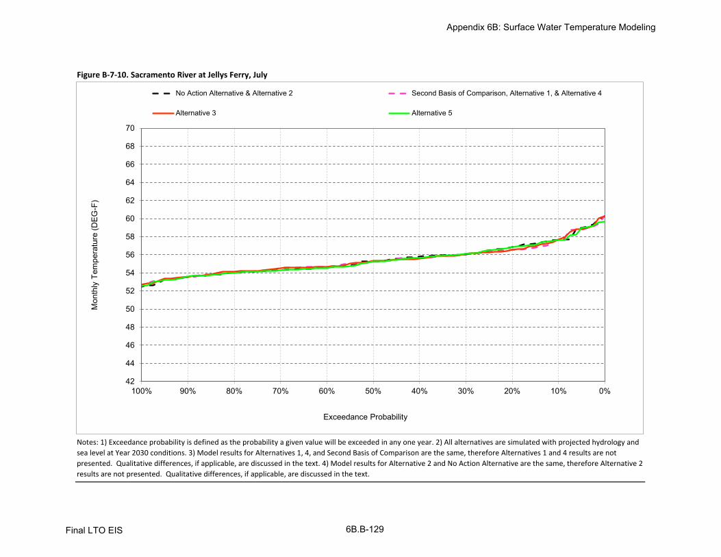
Figure B-7-10. Sacramento River at Jellys Ferry, July
Notes: 1) Exceedance probability is defined as the probability a given value will be exceeded in any one year. 2) All alternatives are simulated with projected hydrology and
sea level at Year 2030 conditions. 3) Model results for Alternatives 1, 4, and Second Basis of Comparison are the same, therefore Alternatives 1 and 4 results are not
presented. Qualitative differences, if applicable, are discussed in the text. 4) Model results for Alternative 2 and No Action Alternative are the same, therefore Alternative 2
results are not presented. Qualitative differences, if applicable, are discussed in the text.
42
44
46
48
50
52
54
56
58
60
62
64
66
68
70
0%10%20%30%40%50%60%70%80%90%100%
Exceedance Probability
No Action Alternative & Alternative 2 Second Basis of Comparison, Alternative 1, & Alternative 4
Alternative 3 Alternative 5
Mon
thly
Tem
pera
ture
(DE
G-F
)
Appendix 6B: Surface Water Temperature Modeling
Final LTO EIS 6B.B-129

Figure B-7-11. Sacramento River at Jellys Ferry, August
Notes: 1) Exceedance probability is defined as the probability a given value will be exceeded in any one year. 2) All alternatives are simulated with projected hydrology and
sea level at Year 2030 conditions. 3) Model results for Alternatives 1, 4, and Second Basis of Comparison are the same, therefore Alternatives 1 and 4 results are not
presented. Qualitative differences, if applicable, are discussed in the text. 4) Model results for Alternative 2 and No Action Alternative are the same, therefore Alternative 2
results are not presented. Qualitative differences, if applicable, are discussed in the text.
42
44
46
48
50
52
54
56
58
60
62
64
66
68
70
0%10%20%30%40%50%60%70%80%90%100%
Exceedance Probability
No Action Alternative & Alternative 2 Second Basis of Comparison, Alternative 1, & Alternative 4
Alternative 3 Alternative 5
Mon
thly
Tem
pera
ture
(DE
G-F
)
Appendix 6B: Surface Water Temperature Modeling
Final LTO EIS 6B.B-130

Figure B-7-12. Sacramento River at Jellys Ferry, September
Notes: 1) Exceedance probability is defined as the probability a given value will be exceeded in any one year. 2) All alternatives are simulated with projected hydrology and
sea level at Year 2030 conditions. 3) Model results for Alternatives 1, 4, and Second Basis of Comparison are the same, therefore Alternatives 1 and 4 results are not
presented. Qualitative differences, if applicable, are discussed in the text. 4) Model results for Alternative 2 and No Action Alternative are the same, therefore Alternative 2
results are not presented. Qualitative differences, if applicable, are discussed in the text.
42
44
46
48
50
52
54
56
58
60
62
64
66
68
70
0%10%20%30%40%50%60%70%80%90%100%
Exceedance Probability
No Action Alternative & Alternative 2 Second Basis of Comparison, Alternative 1, & Alternative 4
Alternative 3 Alternative 5
Mon
thly
Tem
pera
ture
(DE
G-F
)
Appendix 6B: Surface Water Temperature Modeling
Final LTO EIS 6B.B-131
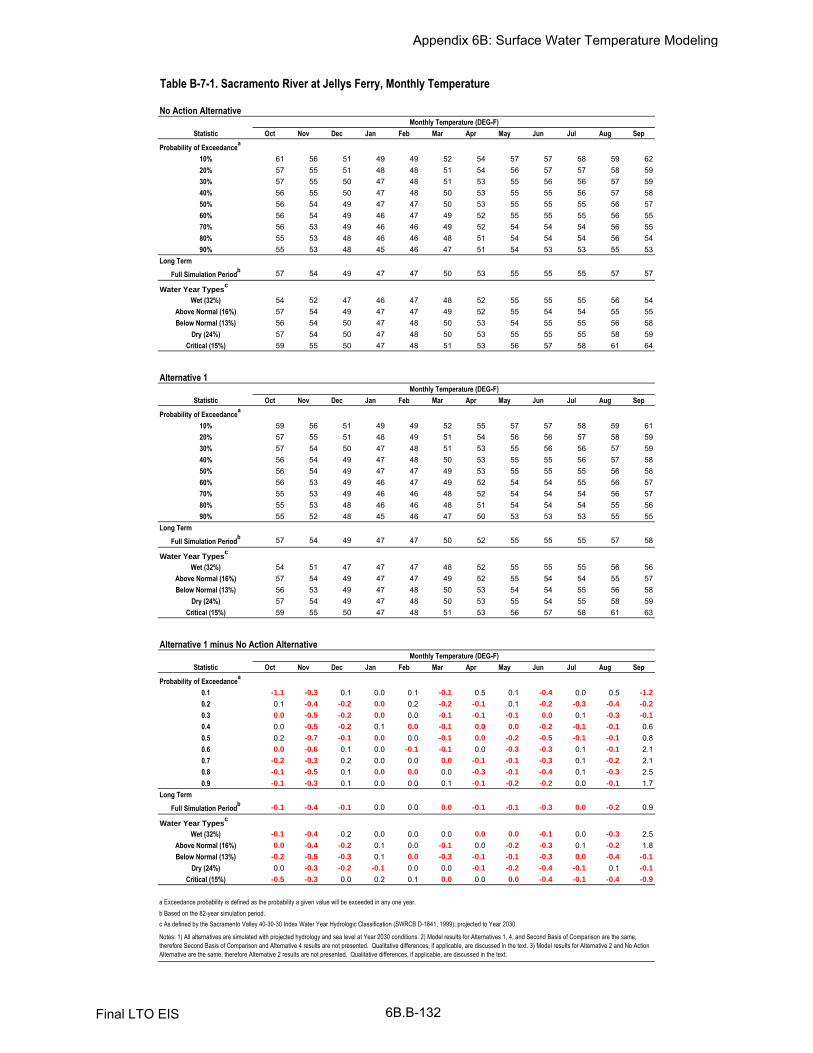
Oct Nov Dec Jan Feb Mar Apr May Jun Jul Aug Sep
10% 61 56 51 49 49 52 54 57 57 58 59 6220% 57 55 51 48 48 51 54 56 57 57 58 5930% 57 55 50 47 48 51 53 55 56 56 57 5940% 56 55 50 47 48 50 53 55 55 56 57 5850% 56 54 49 47 47 50 53 55 55 55 56 5760% 56 54 49 46 47 49 52 55 55 55 56 5570% 56 53 49 46 46 49 52 54 54 54 56 5580% 55 53 48 46 46 48 51 54 54 54 56 5490% 55 53 48 45 46 47 51 54 53 53 55 53
Full Simulation Periodb 57 54 49 47 47 50 53 55 55 55 57 57
Wet (32%) 54 52 47 46 47 48 52 55 55 55 56 54Above Normal (16%) 57 54 49 47 47 49 52 55 54 54 55 55Below Normal (13%) 56 54 50 47 48 50 53 54 55 55 56 58
Dry (24%) 57 54 50 47 48 50 53 55 55 55 58 59Critical (15%) 59 55 50 47 48 51 53 56 57 58 61 64
Oct Nov Dec Jan Feb Mar Apr May Jun Jul Aug Sep
10% 59 56 51 49 49 52 55 57 57 58 59 6120% 57 55 51 48 49 51 54 56 56 57 58 5930% 57 54 50 47 48 51 53 55 56 56 57 5940% 56 54 49 47 48 50 53 55 55 56 57 5850% 56 54 49 47 47 49 53 55 55 55 56 5860% 56 53 49 46 47 49 52 54 54 55 56 5770% 55 53 49 46 46 48 52 54 54 54 56 5780% 55 53 48 46 46 48 51 54 54 54 55 5690% 55 52 48 45 46 47 50 53 53 53 55 55
Full Simulation Periodb 57 54 49 47 47 50 52 55 55 55 57 58
Wet (32%) 54 51 47 47 47 48 52 55 55 55 56 56Above Normal (16%) 57 54 49 47 47 49 52 55 54 54 55 57Below Normal (13%) 56 53 49 47 48 50 53 54 54 55 56 58
Dry (24%) 57 54 49 47 48 50 53 55 54 55 58 59Critical (15%) 59 55 50 47 48 51 53 56 57 58 61 63
Oct Nov Dec Jan Feb Mar Apr May Jun Jul Aug Sep
0.1 -1.1 -0.3 0.1 0.0 0.1 -0.1 0.5 0.1 -0.4 0.0 0.5 -1.2
0.2 0.1 -0.4 -0.2 0.0 0.2 -0.2 -0.1 0.1 -0.2 -0.3 -0.4 -0.2
0.3 0.0 -0.5 -0.2 0.0 0.0 -0.1 -0.1 -0.1 0.0 0.1 -0.3 -0.1
0.4 0.0 -0.5 -0.2 0.1 0.0 -0.1 0.0 0.0 -0.2 -0.1 -0.1 0.60.5 0.2 -0.7 -0.1 0.0 0.0 -0.1 0.0 -0.2 -0.5 -0.1 -0.1 0.80.6 0.0 -0.6 0.1 0.0 -0.1 -0.1 0.0 -0.3 -0.3 0.1 -0.1 2.10.7 -0.2 -0.3 0.2 0.0 0.0 0.0 -0.1 -0.1 -0.3 0.1 -0.2 2.10.8 -0.1 -0.5 0.1 0.0 0.0 0.0 -0.3 -0.1 -0.4 0.1 -0.3 2.50.9 -0.1 -0.3 0.1 0.0 0.0 0.1 -0.1 -0.2 -0.2 0.0 -0.1 1.7
Full Simulation Periodb
-0.1 -0.4 -0.1 0.0 0.0 0.0 -0.1 -0.1 -0.3 0.0 -0.2 0.9
Wet (32%) -0.1 -0.4 0.2 0.0 0.0 0.0 0.0 0.0 -0.1 0.0 -0.3 2.5Above Normal (16%) 0.0 -0.4 -0.2 0.1 0.0 -0.1 0.0 -0.2 -0.3 0.1 -0.2 1.8Below Normal (13%) -0.2 -0.5 -0.3 0.1 0.0 -0.3 -0.1 -0.1 -0.3 0.0 -0.4 -0.1
Dry (24%) 0.0 -0.3 -0.2 -0.1 0.0 0.0 -0.1 -0.2 -0.4 -0.1 0.1 -0.1
Critical (15%) -0.5 -0.3 0.0 0.2 0.1 0.0 0.0 0.0 -0.4 -0.1 -0.4 -0.9
a Exceedance probability is defined as the probability a given value will be exceeded in any one year.
b Based on the 82-year simulation period.
Probability of Exceedancea
Long Term
Water Year Typesc
c As defined by the Sacramento Valley 40-30-30 Index Water Year Hydrologic Classification (SWRCB D-1641, 1999); projected to Year 2030.
Notes: 1) All alternatives are simulated with projected hydrology and sea level at Year 2030 conditions. 2) Model results for Alternatives 1, 4, and Second Basis of Comparison are the same,
therefore Second Basis of Comparison and Alternative 4 results are not presented. Qualitative differences, if applicable, are discussed in the text. 3) Model results for Alternative 2 and No Action
Alternative are the same, therefore Alternative 2 results are not presented. Qualitative differences, if applicable, are discussed in the text.
Probability of Exceedancea
Long Term
Water Year Typesc
Alternative 1 minus No Action Alternative
Statistic
Monthly Temperature (DEG-F)
Long Term
Water Year Typesc
Alternative 1
Statistic
Monthly Temperature (DEG-F)
Table B-7-1. Sacramento River at Jellys Ferry, Monthly Temperature
No Action Alternative
Statistic
Monthly Temperature (DEG-F)
Probability of Exceedancea
Appendix 6B: Surface Water Temperature Modeling
Final LTO EIS 6B.B-132

Oct Nov Dec Jan Feb Mar Apr May Jun Jul Aug Sep
10% 61 56 51 49 49 52 54 57 57 58 59 6220% 57 55 51 48 48 51 54 56 57 57 58 5930% 57 55 50 47 48 51 53 55 56 56 57 5940% 56 55 50 47 48 50 53 55 55 56 57 5850% 56 54 49 47 47 50 53 55 55 55 56 5760% 56 54 49 46 47 49 52 55 55 55 56 5570% 56 53 49 46 46 49 52 54 54 54 56 5580% 55 53 48 46 46 48 51 54 54 54 56 5490% 55 53 48 45 46 47 51 54 53 53 55 53
Full Simulation Periodb 57 54 49 47 47 50 53 55 55 55 57 57
Wet (32%) 54 52 47 46 47 48 52 55 55 55 56 54Above Normal (16%) 57 54 49 47 47 49 52 55 54 54 55 55Below Normal (13%) 56 54 50 47 48 50 53 54 55 55 56 58
Dry (24%) 57 54 50 47 48 50 53 55 55 55 58 59Critical (15%) 59 55 50 47 48 51 53 56 57 58 61 64
Oct Nov Dec Jan Feb Mar Apr May Jun Jul Aug Sep
10% 60 56 51 48 49 52 55 57 57 58 59 6120% 57 55 50 48 48 51 54 56 56 57 58 5930% 57 54 50 47 48 51 53 55 56 56 57 5940% 56 54 49 47 48 50 53 55 55 56 57 5850% 56 54 49 47 47 49 53 55 55 55 56 5760% 56 53 49 47 47 49 52 54 54 55 56 5770% 56 53 49 46 46 48 52 54 54 54 56 5680% 55 53 48 46 46 48 51 54 54 54 55 5690% 55 52 48 45 46 47 51 53 53 54 55 55
Full Simulation Periodb 57 54 49 47 47 50 53 55 55 55 57 58
Wet (32%) 54 51 47 47 47 48 52 55 55 55 56 56Above Normal (16%) 57 54 49 47 47 49 52 55 54 54 55 57Below Normal (13%) 56 53 49 47 48 50 53 54 54 55 56 57
Dry (24%) 56 54 50 47 48 50 53 55 54 55 57 59Critical (15%) 59 55 50 47 48 51 53 56 57 58 61 63
Oct Nov Dec Jan Feb Mar Apr May Jun Jul Aug Sep
0.1 -0.9 -0.2 0.0 -0.1 0.0 -0.1 0.5 0.0 -0.3 0.0 -0.2 -1.2
0.2 0.0 -0.4 -0.2 0.1 0.1 -0.2 -0.1 0.1 -0.2 -0.3 -0.5 -0.4
0.3 0.0 -0.5 0.0 0.0 -0.1 0.0 -0.1 0.0 0.0 0.1 -0.2 -0.1
0.4 0.0 -0.5 -0.2 0.1 0.0 -0.1 -0.1 -0.1 -0.2 -0.2 0.0 0.60.5 0.1 -0.6 -0.2 -0.1 0.1 -0.1 0.0 -0.2 -0.4 0.0 0.0 0.50.6 0.0 -0.6 0.1 0.0 -0.1 0.0 0.0 -0.2 -0.3 0.1 -0.1 2.00.7 0.0 -0.3 0.0 0.1 0.1 0.0 0.0 -0.2 -0.3 0.2 -0.1 1.90.8 -0.2 -0.5 0.0 0.0 0.0 0.0 -0.2 0.0 -0.4 0.1 -0.1 2.00.9 -0.1 -0.2 0.2 0.0 0.0 0.1 0.0 -0.2 -0.2 0.1 -0.1 1.6
Full Simulation Periodb
-0.2 -0.4 0.0 0.0 0.0 0.0 0.0 -0.1 -0.2 0.0 -0.2 0.7
Wet (32%) -0.1 -0.4 0.2 0.0 0.0 0.0 0.0 0.0 -0.1 0.0 -0.2 2.3Above Normal (16%) 0.0 -0.4 -0.2 0.0 0.0 -0.1 0.0 -0.2 -0.2 0.2 0.0 1.9Below Normal (13%) -0.2 -0.6 -0.3 0.1 0.0 -0.2 -0.1 -0.1 -0.2 -0.1 -0.1 -0.9
Dry (24%) -0.1 -0.4 -0.1 -0.1 0.0 0.0 -0.1 -0.1 -0.4 -0.1 -0.2 -0.2
Critical (15%) -0.4 -0.2 0.0 0.1 0.1 0.0 0.1 0.0 -0.3 0.1 -0.5 -1.0
a Exceedance probability is defined as the probability a given value will be exceeded in any one year.
b Based on the 82-year simulation period.
Probability of Exceedancea
Long Term
Water Year Typesc
c As defined by the Sacramento Valley 40-30-30 Index Water Year Hydrologic Classification (SWRCB D-1641, 1999); projected to Year 2030.
Notes: 1) All alternatives are simulated with projected hydrology and sea level at Year 2030 conditions. 2) Model results for Alternatives 1, 4, and Second Basis of Comparison are the same,
therefore Alternative 1 and 4 results are not presented. Qualitative differences, if applicable, are discussed in the text. 3) Model results for Alternative 2 and No Action Alternative are the same,
therefore Alternative 2 results are not presented. Qualitative differences, if applicable, are discussed in the text.
Probability of Exceedancea
Long Term
Water Year Typesc
Alternative 3 minus No Action Alternative
Statistic
Monthly Temperature (DEG-F)
Long Term
Water Year Typesc
Alternative 3
Statistic
Monthly Temperature (DEG-F)
Table B-7-2. Sacramento River at Jellys Ferry, Monthly Temperature
No Action Alternative
Statistic
Monthly Temperature (DEG-F)
Probability of Exceedancea
Appendix 6B: Surface Water Temperature Modeling
Final LTO EIS 6B.B-133
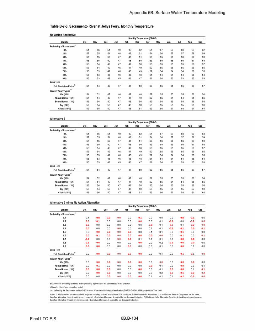
Oct Nov Dec Jan Feb Mar Apr May Jun Jul Aug Sep
10% 61 56 51 49 49 52 54 57 57 58 59 6220% 57 55 51 48 48 51 54 56 57 57 58 5930% 57 55 50 47 48 51 53 55 56 56 57 5940% 56 55 50 47 48 50 53 55 55 56 57 5850% 56 54 49 47 47 50 53 55 55 55 56 5760% 56 54 49 46 47 49 52 55 55 55 56 5570% 56 53 49 46 46 49 52 54 54 54 56 5580% 55 53 48 46 46 48 51 54 54 54 56 5490% 55 53 48 45 46 47 51 54 53 53 55 53
Full Simulation Periodb 57 54 49 47 47 50 53 55 55 55 57 57
Wet (32%) 54 52 47 46 47 48 52 55 55 55 56 54Above Normal (16%) 57 54 49 47 47 49 52 55 54 54 55 55Below Normal (13%) 56 54 50 47 48 50 53 54 55 55 56 58
Dry (24%) 57 54 50 47 48 50 53 55 55 55 58 59Critical (15%) 59 55 50 47 48 51 53 56 57 58 61 64
Oct Nov Dec Jan Feb Mar Apr May Jun Jul Aug Sep
10% 61 56 51 49 49 52 54 57 57 58 59 6320% 57 55 51 48 48 51 54 56 57 57 58 5930% 57 55 50 47 48 51 53 56 56 56 57 5940% 56 55 50 47 48 50 53 55 55 56 57 5850% 56 54 49 47 47 50 53 55 55 55 56 5760% 56 54 49 46 47 49 52 55 55 55 56 5570% 55 53 49 46 46 49 52 54 54 54 56 5580% 55 53 48 46 46 48 51 54 54 54 56 5490% 55 53 48 45 46 47 51 54 53 53 55 53
Full Simulation Periodb 57 54 49 47 47 50 53 55 55 55 57 57
Wet (32%) 54 52 47 46 47 48 52 55 55 55 56 54Above Normal (16%) 57 54 49 47 47 49 52 55 54 54 55 55Below Normal (13%) 56 54 50 47 48 50 53 54 55 55 56 58
Dry (24%) 57 54 50 47 48 50 53 55 55 55 57 59Critical (15%) 59 56 50 47 48 51 53 56 57 58 61 64
Oct Nov Dec Jan Feb Mar Apr May Jun Jul Aug Sep
0.1 0.4 0.0 0.0 0.0 0.0 -0.1 0.0 0.0 0.2 0.0 -0.1 0.60.2 0.0 -0.1 0.0 0.0 0.0 0.0 0.0 0.1 -0.1 0.0 -0.2 0.0
0.3 0.0 0.0 0.0 0.0 0.0 0.0 0.0 0.1 0.0 0.1 -0.2 0.0
0.4 0.0 0.0 0.0 0.0 0.0 0.0 0.1 0.1 -0.1 -0.1 0.0 -0.1
0.5 0.0 0.0 0.0 0.0 0.0 0.0 0.1 0.1 0.0 -0.1 0.0 0.00.6 0.0 -0.1 0.0 0.0 0.0 0.0 0.0 0.0 0.0 -0.1 0.0 -0.1
0.7 -0.2 0.0 0.0 0.0 0.0 0.1 0.1 0.1 0.0 0.0 0.0 0.00.8 -0.1 0.0 0.0 0.0 0.0 0.0 0.0 0.2 -0.1 0.0 0.0 0.00.9 0.0 0.0 0.0 0.0 0.0 0.0 0.0 0.1 0.0 0.0 0.1 0.0
Full Simulation Periodb 0.0 0.0 0.0 0.0 0.0 0.0 0.0 0.1 0.0 -0.1 -0.1 0.0
Wet (32%) 0.0 0.0 0.0 0.0 0.0 0.0 0.0 0.0 0.0 0.0 0.0 0.0Above Normal (16%) 0.0 -0.1 0.0 0.0 0.0 0.0 0.0 0.1 0.0 0.0 0.0 0.1Below Normal (13%) 0.0 0.0 0.0 0.0 0.0 0.0 0.0 0.1 0.0 0.0 0.1 -0.1
Dry (24%) 0.0 0.0 0.0 0.0 0.0 0.0 0.0 0.2 0.0 -0.1 -0.2 -0.2
Critical (15%) 0.0 0.0 0.0 0.0 0.0 0.0 0.1 0.1 0.1 -0.2 -0.2 0.0
a Exceedance probability is defined as the probability a given value will be exceeded in any one year.
b Based on the 82-year simulation period.
Probability of Exceedancea
Long Term
Water Year Typesc
c As defined by the Sacramento Valley 40-30-30 Index Water Year Hydrologic Classification (SWRCB D-1641, 1999); projected to Year 2030.
Notes: 1) All alternatives are simulated with projected hydrology and sea level at Year 2030 conditions. 2) Model results for Alternatives 1, 4, and Second Basis of Comparison are the same,
therefore Alternative 1 and 4 results are not presented. Qualitative differences, if applicable, are discussed in the text. 3) Model results for Alternative 2 and No Action Alternative are the same,
therefore Alternative 2 results are not presented. Qualitative differences, if applicable, are discussed in the text.
Probability of Exceedancea
Long Term
Water Year Typesc
Alternative 5 minus No Action Alternative
Statistic
Monthly Temperature (DEG-F)
Long Term
Water Year Typesc
Alternative 5
Statistic
Monthly Temperature (DEG-F)
Table B-7-3. Sacramento River at Jellys Ferry, Monthly Temperature
No Action Alternative
Statistic
Monthly Temperature (DEG-F)
Probability of Exceedancea
Appendix 6B: Surface Water Temperature Modeling
Final LTO EIS 6B.B-134

Oct Nov Dec Jan Feb Mar Apr May Jun Jul Aug Sep
10% 59 56 51 49 49 52 55 57 57 58 59 6120% 57 55 51 48 49 51 54 56 56 57 58 5930% 57 54 50 47 48 51 53 55 56 56 57 5940% 56 54 49 47 48 50 53 55 55 56 57 5850% 56 54 49 47 47 49 53 55 55 55 56 5860% 56 53 49 46 47 49 52 54 54 55 56 5770% 55 53 49 46 46 48 52 54 54 54 56 5780% 55 53 48 46 46 48 51 54 54 54 55 5690% 55 52 48 45 46 47 50 53 53 53 55 55
Full Simulation Periodb 57 54 49 47 47 50 52 55 55 55 57 58
Wet (32%) 54 51 47 47 47 48 52 55 55 55 56 56Above Normal (16%) 57 54 49 47 47 49 52 55 54 54 55 57Below Normal (13%) 56 53 49 47 48 50 53 54 54 55 56 58
Dry (24%) 57 54 49 47 48 50 53 55 54 55 58 59Critical (15%) 59 55 50 47 48 51 53 56 57 58 61 63
Oct Nov Dec Jan Feb Mar Apr May Jun Jul Aug Sep
10% 61 56 51 49 49 52 54 57 57 58 59 6220% 57 55 51 48 48 51 54 56 57 57 58 5930% 57 55 50 47 48 51 53 55 56 56 57 5940% 56 55 50 47 48 50 53 55 55 56 57 5850% 56 54 49 47 47 50 53 55 55 55 56 5760% 56 54 49 46 47 49 52 55 55 55 56 5570% 56 53 49 46 46 49 52 54 54 54 56 5580% 55 53 48 46 46 48 51 54 54 54 56 5490% 55 53 48 45 46 47 51 54 53 53 55 53
Full Simulation Periodb 57 54 49 47 47 50 53 55 55 55 57 57
Wet (32%) 54 52 47 46 47 48 52 55 55 55 56 54Above Normal (16%) 57 54 49 47 47 49 52 55 54 54 55 55Below Normal (13%) 56 54 50 47 48 50 53 54 55 55 56 58
Dry (24%) 57 54 50 47 48 50 53 55 55 55 58 59Critical (15%) 59 55 50 47 48 51 53 56 57 58 61 64
Oct Nov Dec Jan Feb Mar Apr May Jun Jul Aug Sep
0.1 1.1 0.3 -0.1 0.0 -0.1 0.1 -0.5 -0.1 0.4 0.0 -0.5 1.20.2 -0.1 0.4 0.2 0.0 -0.2 0.2 0.1 -0.1 0.2 0.3 0.4 0.20.3 0.0 0.5 0.2 0.0 0.0 0.1 0.1 0.1 0.0 -0.1 0.3 0.10.4 0.0 0.5 0.2 -0.1 0.0 0.1 0.0 0.0 0.2 0.1 0.1 -0.6
0.5 -0.2 0.7 0.1 0.0 0.0 0.1 0.0 0.2 0.5 0.1 0.1 -0.8
0.6 0.0 0.6 -0.1 0.0 0.1 0.1 0.0 0.3 0.3 -0.1 0.1 -2.1
0.7 0.2 0.3 -0.2 0.0 0.0 0.0 0.1 0.1 0.3 -0.1 0.2 -2.1
0.8 0.1 0.5 -0.1 0.0 0.0 0.0 0.3 0.1 0.4 -0.1 0.3 -2.5
0.9 0.1 0.3 -0.1 0.0 0.0 -0.1 0.1 0.2 0.2 0.0 0.1 -1.7
Full Simulation Periodb 0.1 0.4 0.1 0.0 0.0 0.0 0.1 0.1 0.3 0.0 0.2 -0.9
Wet (32%) 0.1 0.4 -0.2 0.0 0.0 0.0 0.0 0.0 0.1 0.0 0.3 -2.5
Above Normal (16%) 0.0 0.4 0.2 -0.1 0.0 0.1 0.0 0.2 0.3 -0.1 0.2 -1.8
Below Normal (13%) 0.2 0.5 0.3 -0.1 0.0 0.3 0.1 0.1 0.3 0.0 0.4 0.1Dry (24%) 0.0 0.3 0.2 0.1 0.0 0.0 0.1 0.2 0.4 0.1 -0.1 0.1
Critical (15%) 0.5 0.3 0.0 -0.2 -0.1 0.0 0.0 0.0 0.4 0.1 0.4 0.9
a Exceedance probability is defined as the probability a given value will be exceeded in any one year.
b Based on the 82-year simulation period.
Probability of Exceedancea
Long Term
Water Year Typesc
c As defined by the Sacramento Valley 40-30-30 Index Water Year Hydrologic Classification (SWRCB D-1641, 1999); projected to Year 2030.
Notes: 1) All alternatives are simulated with projected hydrology and sea level at Year 2030 conditions. 2) Model results for Alternatives 1, 4, and Second Basis of Comparison are the same,
therefore Alternative 1 and 4 results are not presented. Qualitative differences, if applicable, are discussed in the text. 3) Model results for Alternative 2 and No Action Alternative are the same,
therefore Alternative 2 results are not presented. Qualitative differences, if applicable, are discussed in the text.
Probability of Exceedancea
Long Term
Water Year Typesc
No Action Alternative minus Second Basis of Comparison
Statistic
Monthly Temperature (DEG-F)
Long Term
Water Year Typesc
No Action Alternative
Statistic
Monthly Temperature (DEG-F)
Table B-7-4. Sacramento River at Jellys Ferry, Monthly Temperature
Second Basis of Comparison
Statistic
Monthly Temperature (DEG-F)
Probability of Exceedancea
Appendix 6B: Surface Water Temperature Modeling
Final LTO EIS 6B.B-135

Oct Nov Dec Jan Feb Mar Apr May Jun Jul Aug Sep
10% 59 56 51 49 49 52 55 57 57 58 59 6120% 57 55 51 48 49 51 54 56 56 57 58 5930% 57 54 50 47 48 51 53 55 56 56 57 5940% 56 54 49 47 48 50 53 55 55 56 57 5850% 56 54 49 47 47 49 53 55 55 55 56 5860% 56 53 49 46 47 49 52 54 54 55 56 5770% 55 53 49 46 46 48 52 54 54 54 56 5780% 55 53 48 46 46 48 51 54 54 54 55 5690% 55 52 48 45 46 47 50 53 53 53 55 55
Full Simulation Periodb 57 54 49 47 47 50 52 55 55 55 57 58
Wet (32%) 54 51 47 47 47 48 52 55 55 55 56 56Above Normal (16%) 57 54 49 47 47 49 52 55 54 54 55 57Below Normal (13%) 56 53 49 47 48 50 53 54 54 55 56 58
Dry (24%) 57 54 49 47 48 50 53 55 54 55 58 59Critical (15%) 59 55 50 47 48 51 53 56 57 58 61 63
Oct Nov Dec Jan Feb Mar Apr May Jun Jul Aug Sep
10% 60 56 51 48 49 52 55 57 57 58 59 6120% 57 55 50 48 48 51 54 56 56 57 58 5930% 57 54 50 47 48 51 53 55 56 56 57 5940% 56 54 49 47 48 50 53 55 55 56 57 5850% 56 54 49 47 47 49 53 55 55 55 56 5760% 56 53 49 47 47 49 52 54 54 55 56 5770% 56 53 49 46 46 48 52 54 54 54 56 5680% 55 53 48 46 46 48 51 54 54 54 55 5690% 55 52 48 45 46 47 51 53 53 54 55 55
Full Simulation Periodb 57 54 49 47 47 50 53 55 55 55 57 58
Wet (32%) 54 51 47 47 47 48 52 55 55 55 56 56Above Normal (16%) 57 54 49 47 47 49 52 55 54 54 55 57Below Normal (13%) 56 53 49 47 48 50 53 54 54 55 56 57
Dry (24%) 56 54 50 47 48 50 53 55 54 55 57 59Critical (15%) 59 55 50 47 48 51 53 56 57 58 61 63
Oct Nov Dec Jan Feb Mar Apr May Jun Jul Aug Sep
0.1 0.2 0.1 0.0 -0.1 -0.1 0.0 0.0 -0.1 0.1 0.0 -0.8 -0.1
0.2 -0.1 0.0 0.0 0.1 -0.1 0.0 0.1 0.0 0.1 0.0 0.0 -0.2
0.3 0.0 0.0 0.1 0.0 -0.1 0.0 0.0 0.1 0.0 0.0 0.0 0.0
0.4 0.0 0.0 0.0 0.0 0.0 0.0 -0.1 -0.1 0.0 -0.1 0.1 0.00.5 -0.1 0.2 -0.1 0.0 0.0 0.0 0.1 0.0 0.1 0.1 0.0 -0.2
0.6 0.0 0.0 0.0 0.0 0.0 0.0 0.0 0.0 0.0 0.0 0.0 -0.2
0.7 0.1 0.0 -0.1 0.0 0.1 0.0 0.1 -0.1 0.0 0.0 0.1 -0.2
0.8 -0.1 0.0 0.0 0.1 0.0 0.0 0.1 0.1 0.0 0.1 0.1 -0.5
0.9 0.0 0.0 0.1 0.0 0.0 0.0 0.1 0.0 0.0 0.1 0.0 -0.1
Full Simulation Periodb
0.0 0.0 0.0 0.0 0.0 0.0 0.0 0.0 0.0 0.0 0.0 -0.2
Wet (32%) 0.0 0.0 0.0 0.0 0.0 0.0 0.0 0.0 0.0 0.0 0.2 -0.2
Above Normal (16%) 0.0 0.0 0.0 0.0 0.0 0.0 0.0 0.0 0.1 0.0 0.2 0.0Below Normal (13%) 0.0 0.0 0.0 0.0 0.0 0.0 0.1 0.0 0.1 0.0 0.3 -0.8
Dry (24%) -0.2 -0.1 0.0 0.0 0.0 0.0 0.1 0.0 0.0 0.0 -0.2 -0.1
Critical (15%) 0.1 0.1 0.0 -0.1 -0.1 0.0 0.0 0.0 0.1 0.1 -0.1 -0.1
a Exceedance probability is defined as the probability a given value will be exceeded in any one year.
b Based on the 82-year simulation period.
Probability of Exceedancea
Long Term
Water Year Typesc
c As defined by the Sacramento Valley 40-30-30 Index Water Year Hydrologic Classification (SWRCB D-1641, 1999); projected to Year 2030.
Notes: 1) All alternatives are simulated with projected hydrology and sea level at Year 2030 conditions. 2) Model results for Alternatives 1, 4, and Second Basis of Comparison are the same,
therefore Alternative 1 and 4 results are not presented. Qualitative differences, if applicable, are discussed in the text. 3) Model results for Alternative 2 and No Action Alternative are the same,
therefore Alternative 2 results are not presented. Qualitative differences, if applicable, are discussed in the text.
Probability of Exceedancea
Long Term
Water Year Typesc
Alternative 3 minus Second Basis of Comparison
Statistic
Monthly Temperature (DEG-F)
Long Term
Water Year Typesc
Alternative 3
Statistic
Monthly Temperature (DEG-F)
Table B-7-5. Sacramento River at Jellys Ferry, Monthly Temperature
Second Basis of Comparison
Statistic
Monthly Temperature (DEG-F)
Probability of Exceedancea
Appendix 6B: Surface Water Temperature Modeling
Final LTO EIS 6B.B-136

Oct Nov Dec Jan Feb Mar Apr May Jun Jul Aug Sep
10% 59 56 51 49 49 52 55 57 57 58 59 6120% 57 55 51 48 49 51 54 56 56 57 58 5930% 57 54 50 47 48 51 53 55 56 56 57 5940% 56 54 49 47 48 50 53 55 55 56 57 5850% 56 54 49 47 47 49 53 55 55 55 56 5860% 56 53 49 46 47 49 52 54 54 55 56 5770% 55 53 49 46 46 48 52 54 54 54 56 5780% 55 53 48 46 46 48 51 54 54 54 55 5690% 55 52 48 45 46 47 50 53 53 53 55 55
Full Simulation Periodb 57 54 49 47 47 50 52 55 55 55 57 58
Wet (32%) 54 51 47 47 47 48 52 55 55 55 56 56Above Normal (16%) 57 54 49 47 47 49 52 55 54 54 55 57Below Normal (13%) 56 53 49 47 48 50 53 54 54 55 56 58
Dry (24%) 57 54 49 47 48 50 53 55 54 55 58 59Critical (15%) 59 55 50 47 48 51 53 56 57 58 61 63
Oct Nov Dec Jan Feb Mar Apr May Jun Jul Aug Sep
10% 61 56 51 49 49 52 54 57 57 58 59 6320% 57 55 51 48 48 51 54 56 57 57 58 5930% 57 55 50 47 48 51 53 56 56 56 57 5940% 56 55 50 47 48 50 53 55 55 56 57 5850% 56 54 49 47 47 50 53 55 55 55 56 5760% 56 54 49 46 47 49 52 55 55 55 56 5570% 55 53 49 46 46 49 52 54 54 54 56 5580% 55 53 48 46 46 48 51 54 54 54 56 5490% 55 53 48 45 46 47 51 54 53 53 55 53
Full Simulation Periodb 57 54 49 47 47 50 53 55 55 55 57 57
Wet (32%) 54 52 47 46 47 48 52 55 55 55 56 54Above Normal (16%) 57 54 49 47 47 49 52 55 54 54 55 55Below Normal (13%) 56 54 50 47 48 50 53 54 55 55 56 58
Dry (24%) 57 54 50 47 48 50 53 55 55 55 57 59Critical (15%) 59 56 50 47 48 51 53 56 57 58 61 64
Oct Nov Dec Jan Feb Mar Apr May Jun Jul Aug Sep
0.1 1.5 0.3 -0.1 0.0 -0.1 0.0 -0.4 -0.1 0.5 0.0 -0.6 1.70.2 -0.2 0.3 0.2 0.1 -0.2 0.2 0.2 0.0 0.2 0.3 0.2 0.20.3 0.0 0.5 0.2 0.0 0.0 0.1 0.1 0.2 0.0 0.0 0.1 0.10.4 0.0 0.5 0.2 -0.1 0.0 0.1 0.1 0.1 0.1 0.0 0.1 -0.7
0.5 -0.1 0.7 0.1 0.0 -0.1 0.1 0.1 0.3 0.5 0.0 0.1 -0.8
0.6 0.0 0.5 -0.1 0.0 0.1 0.1 0.0 0.2 0.3 -0.2 0.1 -2.2
0.7 0.0 0.4 -0.2 -0.1 0.0 0.1 0.2 0.3 0.3 -0.2 0.2 -2.0
0.8 0.0 0.5 0.0 0.0 0.1 0.0 0.3 0.3 0.3 -0.1 0.2 -2.5
0.9 0.1 0.3 -0.1 0.0 0.0 -0.1 0.1 0.3 0.2 0.0 0.2 -1.7
Full Simulation Periodb 0.1 0.4 0.0 0.0 0.0 0.0 0.1 0.2 0.3 0.0 0.2 -0.9
Wet (32%) 0.1 0.4 -0.2 0.0 0.0 0.0 0.0 0.0 0.1 -0.1 0.3 -2.5
Above Normal (16%) 0.0 0.3 0.2 -0.1 0.0 0.1 0.0 0.3 0.3 -0.1 0.2 -1.8
Below Normal (13%) 0.2 0.5 0.3 0.0 0.0 0.2 0.1 0.2 0.3 0.0 0.6 0.0Dry (24%) 0.0 0.3 0.2 0.1 0.0 0.0 0.2 0.4 0.4 0.0 -0.3 0.0
Critical (15%) 0.6 0.3 0.0 -0.2 -0.2 0.0 0.1 0.2 0.5 -0.1 0.2 0.9
a Exceedance probability is defined as the probability a given value will be exceeded in any one year.
b Based on the 82-year simulation period.
Probability of Exceedancea
Long Term
Water Year Typesc
c As defined by the Sacramento Valley 40-30-30 Index Water Year Hydrologic Classification (SWRCB D-1641, 1999); projected to Year 2030.
Notes: 1) All alternatives are simulated with projected hydrology and sea level at Year 2030 conditions. 2) Model results for Alternatives 1, 4, and Second Basis of Comparison are the same,
therefore Alternative 1 and 4 results are not presented. Qualitative differences, if applicable, are discussed in the text. 3) Model results for Alternative 2 and No Action Alternative are the same,
therefore Alternative 2 results are not presented. Qualitative differences, if applicable, are discussed in the text.
Probability of Exceedancea
Long Term
Water Year Typesc
Alternative 5 minus Second Basis of Comparison
Statistic
Monthly Temperature (DEG-F)
Long Term
Water Year Typesc
Alternative 5
Statistic
Monthly Temperature (DEG-F)
Table B-7-6. Sacramento River at Jellys Ferry, Monthly Temperature
Second Basis of Comparison
Statistic
Monthly Temperature (DEG-F)
Probability of Exceedancea
Appendix 6B: Surface Water Temperature Modeling
Final LTO EIS 6B.B-137

B.8. Sacramento River at Bend Bridge Temperature
Appendix 6B: Surface Water Temperature Modeling
Final LTO EIS 6B.B-138

Figure B-8-1. Sacramento River at Bend Bridge, October
Notes: 1) Exceedance probability is defined as the probability a given value will be exceeded in any one year. 2) All alternatives are simulated with projected hydrology and
sea level at Year 2030 conditions. 3) Model results for Alternatives 1, 4, and Second Basis of Comparison are the same, therefore Alternatives 1 and 4 results are not
presented. Qualitative differences, if applicable, are discussed in the text. 4) Model results for Alternative 2 and No Action Alternative are the same, therefore Alternative 2
results are not presented. Qualitative differences, if applicable, are discussed in the text.
42
44
46
48
50
52
54
56
58
60
62
64
66
68
70
0%10%20%30%40%50%60%70%80%90%100%
Exceedance Probability
No Action Alternative & Alternative 2 Second Basis of Comparison, Alternative 1, & Alternative 4
Alternative 3 Alternative 5
Mon
thly
Tem
pera
ture
(DE
G-F
)
Appendix 6B: Surface Water Temperature Modeling
Final LTO EIS 6B.B-139

Figure B-8-2. Sacramento River at Bend Bridge, November
Notes: 1) Exceedance probability is defined as the probability a given value will be exceeded in any one year. 2) All alternatives are simulated with projected hydrology and
sea level at Year 2030 conditions. 3) Model results for Alternatives 1, 4, and Second Basis of Comparison are the same, therefore Alternatives 1 and 4 results are not
presented. Qualitative differences, if applicable, are discussed in the text. 4) Model results for Alternative 2 and No Action Alternative are the same, therefore Alternative 2
results are not presented. Qualitative differences, if applicable, are discussed in the text.
42
44
46
48
50
52
54
56
58
60
62
64
66
68
70
0%10%20%30%40%50%60%70%80%90%100%
Exceedance Probability
No Action Alternative & Alternative 2 Second Basis of Comparison, Alternative 1, & Alternative 4
Alternative 3 Alternative 5
Mon
thly
Tem
pera
ture
(DE
G-F
)
Appendix 6B: Surface Water Temperature Modeling
Final LTO EIS 6B.B-140

Figure B-8-3. Sacramento River at Bend Bridge, December
Notes: 1) Exceedance probability is defined as the probability a given value will be exceeded in any one year. 2) All alternatives are simulated with projected hydrology and
sea level at Year 2030 conditions. 3) Model results for Alternatives 1, 4, and Second Basis of Comparison are the same, therefore Alternatives 1 and 4 results are not
presented. Qualitative differences, if applicable, are discussed in the text. 4) Model results for Alternative 2 and No Action Alternative are the same, therefore Alternative 2
results are not presented. Qualitative differences, if applicable, are discussed in the text.
42
44
46
48
50
52
54
56
58
60
62
64
66
68
70
0%10%20%30%40%50%60%70%80%90%100%
Exceedance Probability
No Action Alternative & Alternative 2 Second Basis of Comparison, Alternative 1, & Alternative 4
Alternative 3 Alternative 5
Mon
thly
Tem
pera
ture
(DE
G-F
)
Appendix 6B: Surface Water Temperature Modeling
Final LTO EIS 6B.B-141

Figure B-8-4. Sacramento River at Bend Bridge, January
Notes: 1) Exceedance probability is defined as the probability a given value will be exceeded in any one year. 2) All alternatives are simulated with projected hydrology and
sea level at Year 2030 conditions. 3) Model results for Alternatives 1, 4, and Second Basis of Comparison are the same, therefore Alternatives 1 and 4 results are not
presented. Qualitative differences, if applicable, are discussed in the text. 4) Model results for Alternative 2 and No Action Alternative are the same, therefore Alternative 2
results are not presented. Qualitative differences, if applicable, are discussed in the text.
42
44
46
48
50
52
54
56
58
60
62
64
66
68
70
0%10%20%30%40%50%60%70%80%90%100%
Exceedance Probability
No Action Alternative & Alternative 2 Second Basis of Comparison, Alternative 1, & Alternative 4
Alternative 3 Alternative 5
Mon
thly
Tem
pera
ture
(DE
G-F
)
Appendix 6B: Surface Water Temperature Modeling
Final LTO EIS 6B.B-142

Figure B-8-5. Sacramento River at Bend Bridge, February
Notes: 1) Exceedance probability is defined as the probability a given value will be exceeded in any one year. 2) All alternatives are simulated with projected hydrology and
sea level at Year 2030 conditions. 3) Model results for Alternatives 1, 4, and Second Basis of Comparison are the same, therefore Alternatives 1 and 4 results are not
presented. Qualitative differences, if applicable, are discussed in the text. 4) Model results for Alternative 2 and No Action Alternative are the same, therefore Alternative 2
results are not presented. Qualitative differences, if applicable, are discussed in the text.
42
44
46
48
50
52
54
56
58
60
62
64
66
68
70
0%10%20%30%40%50%60%70%80%90%100%
Exceedance Probability
No Action Alternative & Alternative 2 Second Basis of Comparison, Alternative 1, & Alternative 4
Alternative 3 Alternative 5
Mon
thly
Tem
pera
ture
(DE
G-F
)
Appendix 6B: Surface Water Temperature Modeling
Final LTO EIS 6B.B-143

Figure B-8-6. Sacramento River at Bend Bridge, March
Notes: 1) Exceedance probability is defined as the probability a given value will be exceeded in any one year. 2) All alternatives are simulated with projected hydrology and
sea level at Year 2030 conditions. 3) Model results for Alternatives 1, 4, and Second Basis of Comparison are the same, therefore Alternatives 1 and 4 results are not
presented. Qualitative differences, if applicable, are discussed in the text. 4) Model results for Alternative 2 and No Action Alternative are the same, therefore Alternative 2
results are not presented. Qualitative differences, if applicable, are discussed in the text.
42
44
46
48
50
52
54
56
58
60
62
64
66
68
70
0%10%20%30%40%50%60%70%80%90%100%
Exceedance Probability
No Action Alternative & Alternative 2 Second Basis of Comparison, Alternative 1, & Alternative 4
Alternative 3 Alternative 5
Mon
thly
Tem
pera
ture
(DE
G-F
)
Appendix 6B: Surface Water Temperature Modeling
Final LTO EIS 6B.B-144

Figure B-8-7. Sacramento River at Bend Bridge, April
Notes: 1) Exceedance probability is defined as the probability a given value will be exceeded in any one year. 2) All alternatives are simulated with projected hydrology and
sea level at Year 2030 conditions. 3) Model results for Alternatives 1, 4, and Second Basis of Comparison are the same, therefore Alternatives 1 and 4 results are not
presented. Qualitative differences, if applicable, are discussed in the text. 4) Model results for Alternative 2 and No Action Alternative are the same, therefore Alternative 2
results are not presented. Qualitative differences, if applicable, are discussed in the text.
42
44
46
48
50
52
54
56
58
60
62
64
66
68
70
0%10%20%30%40%50%60%70%80%90%100%
Exceedance Probability
No Action Alternative & Alternative 2 Second Basis of Comparison, Alternative 1, & Alternative 4
Alternative 3 Alternative 5
Mon
thly
Tem
pera
ture
(DE
G-F
)
Appendix 6B: Surface Water Temperature Modeling
Final LTO EIS 6B.B-145

Figure B-8-8. Sacramento River at Bend Bridge, May
Notes: 1) Exceedance probability is defined as the probability a given value will be exceeded in any one year. 2) All alternatives are simulated with projected hydrology and
sea level at Year 2030 conditions. 3) Model results for Alternatives 1, 4, and Second Basis of Comparison are the same, therefore Alternatives 1 and 4 results are not
presented. Qualitative differences, if applicable, are discussed in the text. 4) Model results for Alternative 2 and No Action Alternative are the same, therefore Alternative 2
results are not presented. Qualitative differences, if applicable, are discussed in the text.
42
44
46
48
50
52
54
56
58
60
62
64
66
68
70
0%10%20%30%40%50%60%70%80%90%100%
Exceedance Probability
No Action Alternative & Alternative 2 Second Basis of Comparison, Alternative 1, & Alternative 4
Alternative 3 Alternative 5
Mon
thly
Tem
pera
ture
(DE
G-F
)
Appendix 6B: Surface Water Temperature Modeling
Final LTO EIS 6B.B-146

Figure B-8-9. Sacramento River at Bend Bridge, June
Notes: 1) Exceedance probability is defined as the probability a given value will be exceeded in any one year. 2) All alternatives are simulated with projected hydrology and
sea level at Year 2030 conditions. 3) Model results for Alternatives 1, 4, and Second Basis of Comparison are the same, therefore Alternatives 1 and 4 results are not
presented. Qualitative differences, if applicable, are discussed in the text. 4) Model results for Alternative 2 and No Action Alternative are the same, therefore Alternative 2
results are not presented. Qualitative differences, if applicable, are discussed in the text.
42
44
46
48
50
52
54
56
58
60
62
64
66
68
70
0%10%20%30%40%50%60%70%80%90%100%
Exceedance Probability
No Action Alternative & Alternative 2 Second Basis of Comparison, Alternative 1, & Alternative 4
Alternative 3 Alternative 5
Mon
thly
Tem
pera
ture
(DE
G-F
)
Appendix 6B: Surface Water Temperature Modeling
Final LTO EIS 6B.B-147

Figure B-8-10. Sacramento River at Bend Bridge, July
Notes: 1) Exceedance probability is defined as the probability a given value will be exceeded in any one year. 2) All alternatives are simulated with projected hydrology and
sea level at Year 2030 conditions. 3) Model results for Alternatives 1, 4, and Second Basis of Comparison are the same, therefore Alternatives 1 and 4 results are not
presented. Qualitative differences, if applicable, are discussed in the text. 4) Model results for Alternative 2 and No Action Alternative are the same, therefore Alternative 2
results are not presented. Qualitative differences, if applicable, are discussed in the text.
42
44
46
48
50
52
54
56
58
60
62
64
66
68
70
0%10%20%30%40%50%60%70%80%90%100%
Exceedance Probability
No Action Alternative & Alternative 2 Second Basis of Comparison, Alternative 1, & Alternative 4
Alternative 3 Alternative 5
Mon
thly
Tem
pera
ture
(DE
G-F
)
Appendix 6B: Surface Water Temperature Modeling
Final LTO EIS 6B.B-148

Figure B-8-11. Sacramento River at Bend Bridge, August
Notes: 1) Exceedance probability is defined as the probability a given value will be exceeded in any one year. 2) All alternatives are simulated with projected hydrology and
sea level at Year 2030 conditions. 3) Model results for Alternatives 1, 4, and Second Basis of Comparison are the same, therefore Alternatives 1 and 4 results are not
presented. Qualitative differences, if applicable, are discussed in the text. 4) Model results for Alternative 2 and No Action Alternative are the same, therefore Alternative 2
results are not presented. Qualitative differences, if applicable, are discussed in the text.
42
44
46
48
50
52
54
56
58
60
62
64
66
68
70
0%10%20%30%40%50%60%70%80%90%100%
Exceedance Probability
No Action Alternative & Alternative 2 Second Basis of Comparison, Alternative 1, & Alternative 4
Alternative 3 Alternative 5
Mon
thly
Tem
pera
ture
(DE
G-F
)
Appendix 6B: Surface Water Temperature Modeling
Final LTO EIS 6B.B-149

Figure B-8-12. Sacramento River at Bend Bridge, September
Notes: 1) Exceedance probability is defined as the probability a given value will be exceeded in any one year. 2) All alternatives are simulated with projected hydrology and
sea level at Year 2030 conditions. 3) Model results for Alternatives 1, 4, and Second Basis of Comparison are the same, therefore Alternatives 1 and 4 results are not
presented. Qualitative differences, if applicable, are discussed in the text. 4) Model results for Alternative 2 and No Action Alternative are the same, therefore Alternative 2
results are not presented. Qualitative differences, if applicable, are discussed in the text.
42
44
46
48
50
52
54
56
58
60
62
64
66
68
70
0%10%20%30%40%50%60%70%80%90%100%
Exceedance Probability
No Action Alternative & Alternative 2 Second Basis of Comparison, Alternative 1, & Alternative 4
Alternative 3 Alternative 5
Mon
thly
Tem
pera
ture
(DE
G-F
)
Appendix 6B: Surface Water Temperature Modeling
Final LTO EIS 6B.B-150

Oct Nov Dec Jan Feb Mar Apr May Jun Jul Aug Sep
10% 61 56 51 48 49 52 55 58 58 59 60 6320% 57 55 50 48 48 52 55 57 58 58 59 6030% 57 55 49 47 48 51 54 57 57 57 59 6040% 57 54 49 47 48 51 54 56 57 57 58 5950% 56 54 49 47 47 50 53 56 56 56 58 5860% 56 53 48 46 47 50 53 56 56 56 57 5670% 56 53 48 46 47 49 53 55 55 55 57 5580% 56 53 48 46 46 49 52 55 55 55 57 5590% 55 52 47 46 46 48 51 54 55 55 56 54
Full Simulation Periodb 57 54 49 47 47 50 53 56 56 57 58 58
Wet (32%) 54 51 47 46 47 49 53 56 57 56 57 55Above Normal (16%) 57 54 49 47 47 50 53 56 55 55 57 56Below Normal (13%) 56 54 49 47 48 51 54 55 56 56 57 59
Dry (24%) 57 54 49 47 48 51 54 56 56 57 59 60Critical (15%) 59 55 50 47 48 52 54 57 58 59 62 65
Oct Nov Dec Jan Feb Mar Apr May Jun Jul Aug Sep
10% 60 55 51 48 49 52 55 58 58 59 61 6220% 58 55 50 48 49 52 54 57 57 58 59 6030% 57 54 49 47 48 51 54 56 57 57 58 6040% 57 54 49 47 48 51 54 56 56 57 58 5950% 56 53 49 47 47 50 53 56 56 56 57 5960% 56 53 48 46 47 50 53 55 55 56 57 5970% 56 53 48 46 47 49 53 55 55 56 57 5880% 55 52 48 46 46 48 52 55 55 55 56 5790% 55 52 47 46 46 48 51 54 54 55 56 56
Full Simulation Periodb 57 53 49 47 47 50 53 56 56 57 58 59
Wet (32%) 54 51 47 46 47 49 52 56 56 56 57 57Above Normal (16%) 57 53 49 47 47 50 53 56 55 55 56 58Below Normal (13%) 56 53 49 47 48 51 54 55 55 56 57 59
Dry (24%) 57 53 49 47 48 51 54 56 55 56 59 60Critical (15%) 59 55 50 47 49 52 54 57 58 59 62 64
Oct Nov Dec Jan Feb Mar Apr May Jun Jul Aug Sep
0.1 -1.0 -0.5 -0.2 -0.1 0.0 -0.1 0.2 0.0 -0.1 0.2 0.2 -0.9
0.2 0.1 -0.7 -0.3 0.0 0.0 -0.1 -0.2 0.0 -0.3 -0.2 -0.5 0.0
0.3 0.0 -0.6 0.0 0.1 0.0 0.0 -0.1 -0.1 -0.2 0.0 -0.2 -0.1
0.4 0.1 -0.5 0.0 0.0 0.0 -0.1 0.0 -0.1 -0.3 0.0 -0.2 0.40.5 0.2 -0.8 -0.2 0.0 0.0 -0.1 0.0 -0.1 -0.4 -0.1 -0.1 1.00.6 0.0 -0.4 0.0 0.0 -0.1 0.0 -0.1 -0.3 -0.4 0.2 -0.1 2.40.7 -0.1 -0.1 0.2 0.0 0.0 0.0 -0.2 -0.2 -0.4 0.1 -0.2 2.40.8 -0.1 -0.5 0.1 0.0 0.0 0.0 -0.2 -0.3 -0.4 0.1 -0.3 2.60.9 -0.1 -0.2 0.1 0.0 0.0 0.0 0.0 -0.1 -0.3 -0.1 -0.3 2.0
Full Simulation Periodb
-0.1 -0.4 0.0 0.0 0.0 0.0 -0.1 -0.1 -0.3 0.0 -0.3 1.0
Wet (32%) 0.0 -0.4 0.2 0.0 0.0 0.0 0.0 0.0 -0.1 0.1 -0.4 2.8Above Normal (16%) 0.0 -0.4 -0.2 0.1 0.0 -0.1 0.0 -0.2 -0.3 0.1 -0.2 2.0Below Normal (13%) -0.2 -0.5 -0.3 0.1 0.0 -0.3 -0.2 -0.2 -0.4 0.0 -0.5 -0.1
Dry (24%) 0.0 -0.3 -0.2 0.0 0.0 0.0 -0.2 -0.2 -0.4 -0.1 0.1 -0.1
Critical (15%) -0.5 -0.3 0.0 0.2 0.1 0.0 0.0 0.0 -0.4 0.0 -0.4 -0.8
a Exceedance probability is defined as the probability a given value will be exceeded in any one year.
b Based on the 82-year simulation period.
Probability of Exceedancea
Long Term
Water Year Typesc
c As defined by the Sacramento Valley 40-30-30 Index Water Year Hydrologic Classification (SWRCB D-1641, 1999); projected to Year 2030.
Notes: 1) All alternatives are simulated with projected hydrology and sea level at Year 2030 conditions. 2) Model results for Alternatives 1, 4, and Second Basis of Comparison are the same,
therefore Second Basis of Comparison and Alternative 4 results are not presented. Qualitative differences, if applicable, are discussed in the text. 3) Model results for Alternative 2 and No Action
Alternative are the same, therefore Alternative 2 results are not presented. Qualitative differences, if applicable, are discussed in the text.
Probability of Exceedancea
Long Term
Water Year Typesc
Alternative 1 minus No Action Alternative
Statistic
Monthly Temperature (DEG-F)
Long Term
Water Year Typesc
Alternative 1
Statistic
Monthly Temperature (DEG-F)
Table B-8-1. Sacramento River at Bend Bridge, Monthly Temperature
No Action Alternative
Statistic
Monthly Temperature (DEG-F)
Probability of Exceedancea
Appendix 6B: Surface Water Temperature Modeling
Final LTO EIS 6B.B-151

Oct Nov Dec Jan Feb Mar Apr May Jun Jul Aug Sep
10% 61 56 51 48 49 52 55 58 58 59 60 6320% 57 55 50 48 48 52 55 57 58 58 59 6030% 57 55 49 47 48 51 54 57 57 57 59 6040% 57 54 49 47 48 51 54 56 57 57 58 5950% 56 54 49 47 47 50 53 56 56 56 58 5860% 56 53 48 46 47 50 53 56 56 56 57 5670% 56 53 48 46 47 49 53 55 55 55 57 5580% 56 53 48 46 46 49 52 55 55 55 57 5590% 55 52 47 46 46 48 51 54 55 55 56 54
Full Simulation Periodb 57 54 49 47 47 50 53 56 56 57 58 58
Wet (32%) 54 51 47 46 47 49 53 56 57 56 57 55Above Normal (16%) 57 54 49 47 47 50 53 56 55 55 57 56Below Normal (13%) 56 54 49 47 48 51 54 55 56 56 57 59
Dry (24%) 57 54 49 47 48 51 54 56 56 57 59 60Critical (15%) 59 55 50 47 48 52 54 57 58 59 62 65
Oct Nov Dec Jan Feb Mar Apr May Jun Jul Aug Sep
10% 60 56 51 48 49 52 55 58 58 59 60 6220% 57 55 50 48 49 52 55 57 57 58 59 6030% 57 54 49 47 48 51 54 57 57 57 58 6040% 57 54 49 47 48 51 54 56 56 57 58 5950% 56 53 49 47 47 50 53 56 56 56 58 5960% 56 53 48 46 47 50 53 55 55 56 57 5870% 56 53 48 46 47 49 53 55 55 56 57 5780% 55 52 48 46 46 48 52 55 55 55 57 5790% 55 52 47 46 46 48 51 54 54 55 56 56
Full Simulation Periodb 57 53 49 47 47 50 53 56 56 57 58 59
Wet (32%) 54 51 47 46 47 49 52 56 56 56 57 57Above Normal (16%) 57 53 49 47 47 50 53 56 55 55 57 58Below Normal (13%) 56 53 49 47 48 51 54 55 55 56 57 58
Dry (24%) 57 53 49 47 48 51 54 56 55 56 59 60Critical (15%) 59 55 50 47 48 52 54 57 58 60 62 64
Oct Nov Dec Jan Feb Mar Apr May Jun Jul Aug Sep
0.1 -0.6 -0.1 -0.2 -0.1 0.0 0.0 0.2 -0.1 -0.1 0.2 -0.2 -1.2
0.2 -0.1 -0.6 -0.3 0.0 0.0 0.0 -0.1 0.0 -0.3 -0.3 -0.5 -0.3
0.3 0.0 -0.6 0.0 0.1 -0.1 0.0 -0.1 0.0 -0.1 -0.1 -0.2 -0.1
0.4 0.0 -0.5 0.0 0.0 0.0 -0.1 0.0 -0.1 -0.3 -0.1 -0.2 0.40.5 0.1 -0.8 -0.1 0.0 0.0 -0.1 0.0 0.0 -0.3 -0.1 0.0 0.90.6 0.1 -0.4 0.0 0.0 -0.1 0.0 0.0 -0.3 -0.4 0.0 -0.1 2.00.7 0.0 -0.2 0.1 0.0 0.1 0.0 0.0 -0.2 -0.5 0.1 -0.2 2.10.8 -0.2 -0.5 0.1 0.0 0.0 0.0 -0.1 -0.2 -0.4 0.2 -0.1 2.20.9 -0.2 -0.3 0.1 0.0 0.0 0.0 0.0 -0.2 -0.1 0.1 0.0 1.8
Full Simulation Periodb
-0.1 -0.4 0.0 0.0 0.0 0.0 0.0 -0.1 -0.3 0.0 -0.2 0.8
Wet (32%) -0.1 -0.4 0.2 0.0 0.0 0.0 0.0 0.0 -0.1 0.0 -0.2 2.6Above Normal (16%) 0.0 -0.4 -0.2 0.0 0.0 -0.1 0.0 -0.3 -0.2 0.1 0.0 2.0Below Normal (13%) -0.2 -0.5 -0.3 0.1 0.0 -0.2 -0.1 -0.2 -0.3 -0.1 -0.1 -1.0
Dry (24%) -0.1 -0.4 -0.1 0.0 0.0 0.0 -0.1 -0.1 -0.4 -0.1 -0.2 -0.2
Critical (15%) -0.4 -0.2 0.0 0.1 0.1 0.0 0.1 0.0 -0.3 0.1 -0.5 -0.9
a Exceedance probability is defined as the probability a given value will be exceeded in any one year.
b Based on the 82-year simulation period.
Probability of Exceedancea
Long Term
Water Year Typesc
c As defined by the Sacramento Valley 40-30-30 Index Water Year Hydrologic Classification (SWRCB D-1641, 1999); projected to Year 2030.
Notes: 1) All alternatives are simulated with projected hydrology and sea level at Year 2030 conditions. 2) Model results for Alternatives 1, 4, and Second Basis of Comparison are the same,
therefore Alternative 1 and 4 results are not presented. Qualitative differences, if applicable, are discussed in the text. 3) Model results for Alternative 2 and No Action Alternative are the same,
therefore Alternative 2 results are not presented. Qualitative differences, if applicable, are discussed in the text.
Probability of Exceedancea
Long Term
Water Year Typesc
Alternative 3 minus No Action Alternative
Statistic
Monthly Temperature (DEG-F)
Long Term
Water Year Typesc
Alternative 3
Statistic
Monthly Temperature (DEG-F)
Table B-8-2. Sacramento River at Bend Bridge, Monthly Temperature
No Action Alternative
Statistic
Monthly Temperature (DEG-F)
Probability of Exceedancea
Appendix 6B: Surface Water Temperature Modeling
Final LTO EIS 6B.B-152

Oct Nov Dec Jan Feb Mar Apr May Jun Jul Aug Sep
10% 61 56 51 48 49 52 55 58 58 59 60 6320% 57 55 50 48 48 52 55 57 58 58 59 6030% 57 55 49 47 48 51 54 57 57 57 59 6040% 57 54 49 47 48 51 54 56 57 57 58 5950% 56 54 49 47 47 50 53 56 56 56 58 5860% 56 53 48 46 47 50 53 56 56 56 57 5670% 56 53 48 46 47 49 53 55 55 55 57 5580% 56 53 48 46 46 49 52 55 55 55 57 5590% 55 52 47 46 46 48 51 54 55 55 56 54
Full Simulation Periodb 57 54 49 47 47 50 53 56 56 57 58 58
Wet (32%) 54 51 47 46 47 49 53 56 57 56 57 55Above Normal (16%) 57 54 49 47 47 50 53 56 55 55 57 56Below Normal (13%) 56 54 49 47 48 51 54 55 56 56 57 59
Dry (24%) 57 54 49 47 48 51 54 56 56 57 59 60Critical (15%) 59 55 50 47 48 52 54 57 58 59 62 65
Oct Nov Dec Jan Feb Mar Apr May Jun Jul Aug Sep
10% 61 56 51 48 49 52 55 58 58 59 60 6420% 57 55 50 48 48 52 55 57 57 58 59 6030% 57 55 49 47 48 51 54 57 57 57 58 6040% 57 54 49 47 48 51 54 56 56 57 58 5950% 56 54 49 47 47 50 53 56 56 56 58 5860% 56 53 48 46 47 50 53 56 56 56 57 5670% 56 53 48 46 47 49 53 55 55 55 57 5580% 55 53 48 46 46 49 52 55 55 55 57 5590% 55 52 47 46 46 48 51 54 55 55 56 54
Full Simulation Periodb 57 54 49 47 47 50 53 56 56 56 58 58
Wet (32%) 54 51 47 46 47 49 53 56 57 56 57 55Above Normal (16%) 57 54 49 47 47 50 53 56 55 55 57 56Below Normal (13%) 56 54 49 47 48 51 54 55 56 56 57 59
Dry (24%) 57 54 49 47 48 51 54 56 56 57 59 60Critical (15%) 59 55 50 47 48 52 54 57 58 59 62 65
Oct Nov Dec Jan Feb Mar Apr May Jun Jul Aug Sep
0.1 0.6 -0.1 -0.1 0.0 0.0 0.0 0.0 0.0 0.0 -0.1 -0.6 0.40.2 0.0 -0.1 0.1 0.0 0.0 0.0 -0.1 0.1 -0.1 -0.1 -0.2 -0.1
0.3 0.0 0.0 0.0 0.0 0.0 0.0 0.0 0.1 0.0 0.0 -0.1 0.0
0.4 0.0 0.0 0.0 0.0 0.0 0.0 0.0 0.2 -0.1 0.0 -0.1 -0.3
0.5 0.0 -0.1 0.0 0.0 0.0 0.0 0.0 0.0 0.1 -0.2 0.0 0.10.6 0.0 0.0 0.0 0.0 0.0 0.0 0.1 0.0 0.0 -0.1 0.0 -0.1
0.7 -0.1 0.0 0.0 0.0 0.0 0.0 0.1 0.1 0.0 -0.1 0.0 0.10.8 -0.1 0.0 0.1 0.0 0.0 0.0 0.0 0.1 0.0 0.0 0.0 0.00.9 0.0 0.0 0.0 0.0 0.0 0.0 0.0 0.1 0.0 0.0 0.1 0.0
Full Simulation Periodb 0.0 0.0 0.0 0.0 0.0 0.0 0.0 0.1 0.0 -0.1 -0.1 0.0
Wet (32%) 0.0 0.0 0.0 0.0 0.0 0.0 0.0 0.0 0.0 0.0 0.0 0.0Above Normal (16%) 0.0 -0.1 0.0 0.0 0.0 0.0 0.0 0.1 0.0 0.0 0.0 0.1Below Normal (13%) 0.0 0.0 0.0 0.0 0.0 0.0 0.0 0.1 0.0 0.0 0.2 -0.1
Dry (24%) 0.0 0.0 0.0 0.0 0.0 0.0 0.0 0.2 0.0 -0.1 -0.3 -0.2
Critical (15%) 0.0 0.0 0.0 0.0 0.0 0.0 0.1 0.2 0.1 -0.2 -0.2 0.0
a Exceedance probability is defined as the probability a given value will be exceeded in any one year.
b Based on the 82-year simulation period.
Probability of Exceedancea
Long Term
Water Year Typesc
c As defined by the Sacramento Valley 40-30-30 Index Water Year Hydrologic Classification (SWRCB D-1641, 1999); projected to Year 2030.
Notes: 1) All alternatives are simulated with projected hydrology and sea level at Year 2030 conditions. 2) Model results for Alternatives 1, 4, and Second Basis of Comparison are the same,
therefore Alternative 1 and 4 results are not presented. Qualitative differences, if applicable, are discussed in the text. 3) Model results for Alternative 2 and No Action Alternative are the same,
therefore Alternative 2 results are not presented. Qualitative differences, if applicable, are discussed in the text.
Probability of Exceedancea
Long Term
Water Year Typesc
Alternative 5 minus No Action Alternative
Statistic
Monthly Temperature (DEG-F)
Long Term
Water Year Typesc
Alternative 5
Statistic
Monthly Temperature (DEG-F)
Table B-8-3. Sacramento River at Bend Bridge, Monthly Temperature
No Action Alternative
Statistic
Monthly Temperature (DEG-F)
Probability of Exceedancea
Appendix 6B: Surface Water Temperature Modeling
Final LTO EIS 6B.B-153

Oct Nov Dec Jan Feb Mar Apr May Jun Jul Aug Sep
10% 60 55 51 48 49 52 55 58 58 59 61 6220% 58 55 50 48 49 52 54 57 57 58 59 6030% 57 54 49 47 48 51 54 56 57 57 58 6040% 57 54 49 47 48 51 54 56 56 57 58 5950% 56 53 49 47 47 50 53 56 56 56 57 5960% 56 53 48 46 47 50 53 55 55 56 57 5970% 56 53 48 46 47 49 53 55 55 56 57 5880% 55 52 48 46 46 48 52 55 55 55 56 5790% 55 52 47 46 46 48 51 54 54 55 56 56
Full Simulation Periodb 57 53 49 47 47 50 53 56 56 57 58 59
Wet (32%) 54 51 47 46 47 49 52 56 56 56 57 57Above Normal (16%) 57 53 49 47 47 50 53 56 55 55 56 58Below Normal (13%) 56 53 49 47 48 51 54 55 55 56 57 59
Dry (24%) 57 53 49 47 48 51 54 56 55 56 59 60Critical (15%) 59 55 50 47 49 52 54 57 58 59 62 64
Oct Nov Dec Jan Feb Mar Apr May Jun Jul Aug Sep
10% 61 56 51 48 49 52 55 58 58 59 60 6320% 57 55 50 48 48 52 55 57 58 58 59 6030% 57 55 49 47 48 51 54 57 57 57 59 6040% 57 54 49 47 48 51 54 56 57 57 58 5950% 56 54 49 47 47 50 53 56 56 56 58 5860% 56 53 48 46 47 50 53 56 56 56 57 5670% 56 53 48 46 47 49 53 55 55 55 57 5580% 56 53 48 46 46 49 52 55 55 55 57 5590% 55 52 47 46 46 48 51 54 55 55 56 54
Full Simulation Periodb 57 54 49 47 47 50 53 56 56 57 58 58
Wet (32%) 54 51 47 46 47 49 53 56 57 56 57 55Above Normal (16%) 57 54 49 47 47 50 53 56 55 55 57 56Below Normal (13%) 56 54 49 47 48 51 54 55 56 56 57 59
Dry (24%) 57 54 49 47 48 51 54 56 56 57 59 60Critical (15%) 59 55 50 47 48 52 54 57 58 59 62 65
Oct Nov Dec Jan Feb Mar Apr May Jun Jul Aug Sep
0.1 1.0 0.5 0.2 0.1 0.0 0.1 -0.2 0.0 0.1 -0.2 -0.2 0.90.2 -0.1 0.7 0.3 0.0 0.0 0.1 0.2 0.0 0.3 0.2 0.5 0.00.3 0.0 0.6 0.0 -0.1 0.0 0.0 0.1 0.1 0.2 0.0 0.2 0.10.4 -0.1 0.5 0.0 0.0 0.0 0.1 0.0 0.1 0.3 0.0 0.2 -0.4
0.5 -0.2 0.8 0.2 0.0 0.0 0.1 0.0 0.1 0.4 0.1 0.1 -1.0
0.6 0.0 0.4 0.0 0.0 0.1 0.0 0.1 0.3 0.4 -0.2 0.1 -2.4
0.7 0.1 0.1 -0.2 0.0 0.0 0.0 0.2 0.2 0.4 -0.1 0.2 -2.4
0.8 0.1 0.5 -0.1 0.0 0.0 0.0 0.2 0.3 0.4 -0.1 0.3 -2.6
0.9 0.1 0.2 -0.1 0.0 0.0 0.0 0.0 0.1 0.3 0.1 0.3 -2.0
Full Simulation Periodb 0.1 0.4 0.0 0.0 0.0 0.0 0.1 0.1 0.3 0.0 0.3 -1.0
Wet (32%) 0.0 0.4 -0.2 0.0 0.0 0.0 0.0 0.0 0.1 -0.1 0.4 -2.8
Above Normal (16%) 0.0 0.4 0.2 -0.1 0.0 0.1 0.0 0.2 0.3 -0.1 0.2 -2.0
Below Normal (13%) 0.2 0.5 0.3 -0.1 0.0 0.3 0.2 0.2 0.4 0.0 0.5 0.1Dry (24%) 0.0 0.3 0.2 0.0 0.0 0.0 0.2 0.2 0.4 0.1 -0.1 0.1
Critical (15%) 0.5 0.3 0.0 -0.2 -0.1 0.0 0.0 0.0 0.4 0.0 0.4 0.8
a Exceedance probability is defined as the probability a given value will be exceeded in any one year.
b Based on the 82-year simulation period.
Probability of Exceedancea
Long Term
Water Year Typesc
c As defined by the Sacramento Valley 40-30-30 Index Water Year Hydrologic Classification (SWRCB D-1641, 1999); projected to Year 2030.
Notes: 1) All alternatives are simulated with projected hydrology and sea level at Year 2030 conditions. 2) Model results for Alternatives 1, 4, and Second Basis of Comparison are the same,
therefore Alternative 1 and 4 results are not presented. Qualitative differences, if applicable, are discussed in the text. 3) Model results for Alternative 2 and No Action Alternative are the same,
therefore Alternative 2 results are not presented. Qualitative differences, if applicable, are discussed in the text.
Probability of Exceedancea
Long Term
Water Year Typesc
No Action Alternative minus Second Basis of Comparison
Statistic
Monthly Temperature (DEG-F)
Long Term
Water Year Typesc
No Action Alternative
Statistic
Monthly Temperature (DEG-F)
Table B-8-4. Sacramento River at Bend Bridge, Monthly Temperature
Second Basis of Comparison
Statistic
Monthly Temperature (DEG-F)
Probability of Exceedancea
Appendix 6B: Surface Water Temperature Modeling
Final LTO EIS 6B.B-154

Oct Nov Dec Jan Feb Mar Apr May Jun Jul Aug Sep
10% 60 55 51 48 49 52 55 58 58 59 61 6220% 58 55 50 48 49 52 54 57 57 58 59 6030% 57 54 49 47 48 51 54 56 57 57 58 6040% 57 54 49 47 48 51 54 56 56 57 58 5950% 56 53 49 47 47 50 53 56 56 56 57 5960% 56 53 48 46 47 50 53 55 55 56 57 5970% 56 53 48 46 47 49 53 55 55 56 57 5880% 55 52 48 46 46 48 52 55 55 55 56 5790% 55 52 47 46 46 48 51 54 54 55 56 56
Full Simulation Periodb 57 53 49 47 47 50 53 56 56 57 58 59
Wet (32%) 54 51 47 46 47 49 52 56 56 56 57 57Above Normal (16%) 57 53 49 47 47 50 53 56 55 55 56 58Below Normal (13%) 56 53 49 47 48 51 54 55 55 56 57 59
Dry (24%) 57 53 49 47 48 51 54 56 55 56 59 60Critical (15%) 59 55 50 47 49 52 54 57 58 59 62 64
Oct Nov Dec Jan Feb Mar Apr May Jun Jul Aug Sep
10% 60 56 51 48 49 52 55 58 58 59 60 6220% 57 55 50 48 49 52 55 57 57 58 59 6030% 57 54 49 47 48 51 54 57 57 57 58 6040% 57 54 49 47 48 51 54 56 56 57 58 5950% 56 53 49 47 47 50 53 56 56 56 58 5960% 56 53 48 46 47 50 53 55 55 56 57 5870% 56 53 48 46 47 49 53 55 55 56 57 5780% 55 52 48 46 46 48 52 55 55 55 57 5790% 55 52 47 46 46 48 51 54 54 55 56 56
Full Simulation Periodb 57 53 49 47 47 50 53 56 56 57 58 59
Wet (32%) 54 51 47 46 47 49 52 56 56 56 57 57Above Normal (16%) 57 53 49 47 47 50 53 56 55 55 57 58Below Normal (13%) 56 53 49 47 48 51 54 55 55 56 57 58
Dry (24%) 57 53 49 47 48 51 54 56 55 56 59 60Critical (15%) 59 55 50 47 48 52 54 57 58 60 62 64
Oct Nov Dec Jan Feb Mar Apr May Jun Jul Aug Sep
0.1 0.4 0.4 0.0 0.0 0.0 0.0 0.0 -0.1 0.1 0.0 -0.4 -0.3
0.2 -0.2 0.1 0.0 0.0 0.0 0.0 0.1 0.0 0.0 -0.1 0.0 -0.3
0.3 0.0 0.0 0.0 0.0 -0.1 0.0 0.0 0.0 0.0 -0.1 0.0 0.0
0.4 0.0 0.0 0.1 0.0 0.1 0.0 0.0 0.0 0.0 -0.1 0.0 0.00.5 -0.1 0.0 0.0 0.0 0.0 0.0 0.0 0.0 0.1 0.1 0.2 -0.1
0.6 0.0 0.0 0.0 0.0 0.0 0.0 0.1 0.0 0.0 -0.1 0.0 -0.4
0.7 0.1 0.0 -0.1 0.0 0.1 0.0 0.2 0.0 0.0 0.0 0.1 -0.3
0.8 -0.1 0.0 0.0 0.0 0.0 0.0 0.1 0.1 0.0 0.1 0.2 -0.4
0.9 -0.1 -0.1 0.0 0.0 0.0 0.0 0.0 -0.1 0.3 0.2 0.3 -0.2
Full Simulation Periodb
-0.1 0.0 0.0 0.0 0.0 0.0 0.0 0.0 0.0 0.0 0.0 -0.2
Wet (32%) 0.0 0.0 0.0 0.0 0.0 0.0 0.0 0.0 -0.1 0.0 0.2 -0.2
Above Normal (16%) 0.0 0.0 0.0 0.0 0.0 0.0 0.0 0.0 0.1 0.0 0.2 0.0Below Normal (13%) 0.0 0.0 0.0 0.0 0.0 0.0 0.1 0.0 0.1 0.0 0.3 -0.9
Dry (24%) -0.2 -0.1 0.1 0.0 0.0 0.0 0.1 0.0 0.0 0.0 -0.3 -0.1
Critical (15%) 0.0 0.1 0.0 -0.1 -0.1 0.0 0.0 0.0 0.1 0.1 -0.2 -0.1
a Exceedance probability is defined as the probability a given value will be exceeded in any one year.
b Based on the 82-year simulation period.
Probability of Exceedancea
Long Term
Water Year Typesc
c As defined by the Sacramento Valley 40-30-30 Index Water Year Hydrologic Classification (SWRCB D-1641, 1999); projected to Year 2030.
Notes: 1) All alternatives are simulated with projected hydrology and sea level at Year 2030 conditions. 2) Model results for Alternatives 1, 4, and Second Basis of Comparison are the same,
therefore Alternative 1 and 4 results are not presented. Qualitative differences, if applicable, are discussed in the text. 3) Model results for Alternative 2 and No Action Alternative are the same,
therefore Alternative 2 results are not presented. Qualitative differences, if applicable, are discussed in the text.
Probability of Exceedancea
Long Term
Water Year Typesc
Alternative 3 minus Second Basis of Comparison
Statistic
Monthly Temperature (DEG-F)
Long Term
Water Year Typesc
Alternative 3
Statistic
Monthly Temperature (DEG-F)
Table B-8-5. Sacramento River at Bend Bridge, Monthly Temperature
Second Basis of Comparison
Statistic
Monthly Temperature (DEG-F)
Probability of Exceedancea
Appendix 6B: Surface Water Temperature Modeling
Final LTO EIS 6B.B-155

Oct Nov Dec Jan Feb Mar Apr May Jun Jul Aug Sep
10% 60 55 51 48 49 52 55 58 58 59 61 6220% 58 55 50 48 49 52 54 57 57 58 59 6030% 57 54 49 47 48 51 54 56 57 57 58 6040% 57 54 49 47 48 51 54 56 56 57 58 5950% 56 53 49 47 47 50 53 56 56 56 57 5960% 56 53 48 46 47 50 53 55 55 56 57 5970% 56 53 48 46 47 49 53 55 55 56 57 5880% 55 52 48 46 46 48 52 55 55 55 56 5790% 55 52 47 46 46 48 51 54 54 55 56 56
Full Simulation Periodb 57 53 49 47 47 50 53 56 56 57 58 59
Wet (32%) 54 51 47 46 47 49 52 56 56 56 57 57Above Normal (16%) 57 53 49 47 47 50 53 56 55 55 56 58Below Normal (13%) 56 53 49 47 48 51 54 55 55 56 57 59
Dry (24%) 57 53 49 47 48 51 54 56 55 56 59 60Critical (15%) 59 55 50 47 49 52 54 57 58 59 62 64
Oct Nov Dec Jan Feb Mar Apr May Jun Jul Aug Sep
10% 61 56 51 48 49 52 55 58 58 59 60 6420% 57 55 50 48 48 52 55 57 57 58 59 6030% 57 55 49 47 48 51 54 57 57 57 58 6040% 57 54 49 47 48 51 54 56 56 57 58 5950% 56 54 49 47 47 50 53 56 56 56 58 5860% 56 53 48 46 47 50 53 56 56 56 57 5670% 56 53 48 46 47 49 53 55 55 55 57 5580% 55 53 48 46 46 49 52 55 55 55 57 5590% 55 52 47 46 46 48 51 54 55 55 56 54
Full Simulation Periodb 57 54 49 47 47 50 53 56 56 56 58 58
Wet (32%) 54 51 47 46 47 49 53 56 57 56 57 55Above Normal (16%) 57 54 49 47 47 50 53 56 55 55 57 56Below Normal (13%) 56 54 49 47 48 51 54 55 56 56 57 59
Dry (24%) 57 54 49 47 48 51 54 56 56 57 59 60Critical (15%) 59 55 50 47 48 52 54 57 58 59 62 65
Oct Nov Dec Jan Feb Mar Apr May Jun Jul Aug Sep
0.1 1.6 0.4 0.1 0.1 0.0 0.1 -0.2 0.0 0.1 -0.3 -0.8 1.30.2 -0.1 0.6 0.4 0.0 0.0 0.0 0.1 0.1 0.2 0.1 0.3 -0.1
0.3 0.0 0.6 0.0 -0.1 0.0 0.0 0.1 0.1 0.1 0.1 0.1 0.10.4 -0.1 0.5 0.0 -0.1 0.0 0.1 0.0 0.2 0.2 -0.1 0.1 -0.7
0.5 -0.2 0.7 0.1 0.0 0.0 0.1 0.0 0.1 0.5 0.0 0.2 -0.9
0.6 -0.1 0.4 0.0 0.0 0.1 0.0 0.1 0.3 0.4 -0.2 0.1 -2.5
0.7 0.0 0.2 -0.2 0.0 0.0 0.0 0.3 0.3 0.4 -0.1 0.2 -2.4
0.8 0.0 0.5 0.0 0.0 0.0 0.0 0.2 0.4 0.4 -0.1 0.2 -2.5
0.9 0.1 0.2 -0.1 0.0 0.0 0.0 0.0 0.2 0.4 0.1 0.4 -2.0
Full Simulation Periodb 0.1 0.4 0.0 0.0 0.0 0.0 0.1 0.2 0.3 0.0 0.2 -1.1
Wet (32%) 0.1 0.4 -0.2 0.0 0.0 0.0 0.0 0.0 0.1 -0.1 0.4 -2.8
Above Normal (16%) 0.0 0.3 0.2 -0.1 0.0 0.1 0.0 0.3 0.3 -0.1 0.2 -2.0
Below Normal (13%) 0.2 0.5 0.3 -0.1 0.0 0.2 0.2 0.2 0.4 0.0 0.6 0.0Dry (24%) 0.0 0.3 0.1 0.1 0.0 0.0 0.2 0.4 0.4 0.1 -0.3 0.0
Critical (15%) 0.5 0.3 0.0 -0.2 -0.2 0.0 0.1 0.2 0.5 -0.2 0.1 0.8
a Exceedance probability is defined as the probability a given value will be exceeded in any one year.
b Based on the 82-year simulation period.
Probability of Exceedancea
Long Term
Water Year Typesc
c As defined by the Sacramento Valley 40-30-30 Index Water Year Hydrologic Classification (SWRCB D-1641, 1999); projected to Year 2030.
Notes: 1) All alternatives are simulated with projected hydrology and sea level at Year 2030 conditions. 2) Model results for Alternatives 1, 4, and Second Basis of Comparison are the same,
therefore Alternative 1 and 4 results are not presented. Qualitative differences, if applicable, are discussed in the text. 3) Model results for Alternative 2 and No Action Alternative are the same,
therefore Alternative 2 results are not presented. Qualitative differences, if applicable, are discussed in the text.
Probability of Exceedancea
Long Term
Water Year Typesc
Alternative 5 minus Second Basis of Comparison
Statistic
Monthly Temperature (DEG-F)
Long Term
Water Year Typesc
Alternative 5
Statistic
Monthly Temperature (DEG-F)
Table B-8-6. Sacramento River at Bend Bridge, Monthly Temperature
Second Basis of Comparison
Statistic
Monthly Temperature (DEG-F)
Probability of Exceedancea
Appendix 6B: Surface Water Temperature Modeling
Final LTO EIS 6B.B-156

B.9. Sacramento River at Red Bluff Temperature
Appendix 6B: Surface Water Temperature Modeling
6B.B-157

Figure B-9-1. Sacramento River at Red Bluff, October
Notes: 1) Exceedance probability is defined as the probability a given value will be exceeded in any one year. 2) All alternatives are simulated with projected hydrology and
sea level at Year 2030 conditions. 3) Model results for Alternatives 1, 4, and Second Basis of Comparison are the same, therefore Alternatives 1 and 4 results are not
presented. Qualitative differences, if applicable, are discussed in the text. 4) Model results for Alternative 2 and No Action Alternative are the same, therefore Alternative 2
results are not presented. Qualitative differences, if applicable, are discussed in the text.
42
44
46
48
50
52
54
56
58
60
62
64
66
68
70
72
0%10%20%30%40%50%60%70%80%90%100%
Exceedance Probability
No Action Alternative & Alternative 2 Second Basis of Comparison, Alternative 1, & Alternative 4
Alternative 3 Alternative 5
Mon
thly
Tem
pera
ture
(DE
G-F
)
Appendix 6B: Surface Water Temperature Modeling
Final LTO EIS6B.B-158

Figure B-9-2. Sacramento River at Red Bluff, November
Notes: 1) Exceedance probability is defined as the probability a given value will be exceeded in any one year. 2) All alternatives are simulated with projected hydrology and
sea level at Year 2030 conditions. 3) Model results for Alternatives 1, 4, and Second Basis of Comparison are the same, therefore Alternatives 1 and 4 results are not
presented. Qualitative differences, if applicable, are discussed in the text. 4) Model results for Alternative 2 and No Action Alternative are the same, therefore Alternative 2
results are not presented. Qualitative differences, if applicable, are discussed in the text.
42
44
46
48
50
52
54
56
58
60
62
64
66
68
70
72
0%10%20%30%40%50%60%70%80%90%100%
Exceedance Probability
No Action Alternative & Alternative 2 Second Basis of Comparison, Alternative 1, & Alternative 4
Alternative 3 Alternative 5
Mon
thly
Tem
pera
ture
(DE
G-F
)
Appendix 6B: Surface Water Temperature Modeling
Final LTO EIS6B.B-159

Figure B-9-3. Sacramento River at Red Bluff, December
Notes: 1) Exceedance probability is defined as the probability a given value will be exceeded in any one year. 2) All alternatives are simulated with projected hydrology and
sea level at Year 2030 conditions. 3) Model results for Alternatives 1, 4, and Second Basis of Comparison are the same, therefore Alternatives 1 and 4 results are not
presented. Qualitative differences, if applicable, are discussed in the text. 4) Model results for Alternative 2 and No Action Alternative are the same, therefore Alternative 2
results are not presented. Qualitative differences, if applicable, are discussed in the text.
42
44
46
48
50
52
54
56
58
60
62
64
66
68
70
72
0%10%20%30%40%50%60%70%80%90%100%
Exceedance Probability
No Action Alternative & Alternative 2 Second Basis of Comparison, Alternative 1, & Alternative 4
Alternative 3 Alternative 5
Mon
thly
Tem
pera
ture
(DE
G-F
)
Appendix 6B: Surface Water Temperature Modeling
6B.B-160

Figure B-9-4. Sacramento River at Red Bluff, January
Notes: 1) Exceedance probability is defined as the probability a given value will be exceeded in any one year. 2) All alternatives are simulated with projected hydrology and
sea level at Year 2030 conditions. 3) Model results for Alternatives 1, 4, and Second Basis of Comparison are the same, therefore Alternatives 1 and 4 results are not
presented. Qualitative differences, if applicable, are discussed in the text. 4) Model results for Alternative 2 and No Action Alternative are the same, therefore Alternative 2
results are not presented. Qualitative differences, if applicable, are discussed in the text.
42
44
46
48
50
52
54
56
58
60
62
64
66
68
70
72
0%10%20%30%40%50%60%70%80%90%100%
Exceedance Probability
No Action Alternative & Alternative 2 Second Basis of Comparison, Alternative 1, & Alternative 4
Alternative 3 Alternative 5
Mon
thly
Tem
pera
ture
(DE
G-F
)
Appendix 6B: Surface Water Temperature Modeling
6B.B-161

Figure B-9-5. Sacramento River at Red Bluff, February
Notes: 1) Exceedance probability is defined as the probability a given value will be exceeded in any one year. 2) All alternatives are simulated with projected hydrology and
sea level at Year 2030 conditions. 3) Model results for Alternatives 1, 4, and Second Basis of Comparison are the same, therefore Alternatives 1 and 4 results are not
presented. Qualitative differences, if applicable, are discussed in the text. 4) Model results for Alternative 2 and No Action Alternative are the same, therefore Alternative 2
results are not presented. Qualitative differences, if applicable, are discussed in the text.
42
44
46
48
50
52
54
56
58
60
62
64
66
68
70
72
0%10%20%30%40%50%60%70%80%90%100%
Exceedance Probability
No Action Alternative & Alternative 2 Second Basis of Comparison, Alternative 1, & Alternative 4
Alternative 3 Alternative 5
Mon
thly
Tem
pera
ture
(DE
G-F
)
Appendix 6B: Surface Water Temperature Modeling
6B.B-162

Figure B-9-6. Sacramento River at Red Bluff, March
Notes: 1) Exceedance probability is defined as the probability a given value will be exceeded in any one year. 2) All alternatives are simulated with projected hydrology and
sea level at Year 2030 conditions. 3) Model results for Alternatives 1, 4, and Second Basis of Comparison are the same, therefore Alternatives 1 and 4 results are not
presented. Qualitative differences, if applicable, are discussed in the text. 4) Model results for Alternative 2 and No Action Alternative are the same, therefore Alternative 2
results are not presented. Qualitative differences, if applicable, are discussed in the text.
42
44
46
48
50
52
54
56
58
60
62
64
66
68
70
72
0%10%20%30%40%50%60%70%80%90%100%
Exceedance Probability
No Action Alternative & Alternative 2 Second Basis of Comparison, Alternative 1, & Alternative 4
Alternative 3 Alternative 5
Mon
thly
Tem
pera
ture
(DE
G-F
)
Appendix 6B: Surface Water Temperature Modeling
6B.B-163

Figure B-9-7. Sacramento River at Red Bluff, April
Notes: 1) Exceedance probability is defined as the probability a given value will be exceeded in any one year. 2) All alternatives are simulated with projected hydrology and
sea level at Year 2030 conditions. 3) Model results for Alternatives 1, 4, and Second Basis of Comparison are the same, therefore Alternatives 1 and 4 results are not
presented. Qualitative differences, if applicable, are discussed in the text. 4) Model results for Alternative 2 and No Action Alternative are the same, therefore Alternative 2
results are not presented. Qualitative differences, if applicable, are discussed in the text.
42
44
46
48
50
52
54
56
58
60
62
64
66
68
70
72
0%10%20%30%40%50%60%70%80%90%100%
Exceedance Probability
No Action Alternative & Alternative 2 Second Basis of Comparison, Alternative 1, & Alternative 4
Alternative 3 Alternative 5
Mon
thly
Tem
pera
ture
(DE
G-F
)
Appendix 6B: Surface Water Temperature Modeling
6B.B-164

Figure B-9-8. Sacramento River at Red Bluff, May
Notes: 1) Exceedance probability is defined as the probability a given value will be exceeded in any one year. 2) All alternatives are simulated with projected hydrology and
sea level at Year 2030 conditions. 3) Model results for Alternatives 1, 4, and Second Basis of Comparison are the same, therefore Alternatives 1 and 4 results are not
presented. Qualitative differences, if applicable, are discussed in the text. 4) Model results for Alternative 2 and No Action Alternative are the same, therefore Alternative 2
results are not presented. Qualitative differences, if applicable, are discussed in the text.
42
44
46
48
50
52
54
56
58
60
62
64
66
68
70
72
0%10%20%30%40%50%60%70%80%90%100%
Exceedance Probability
No Action Alternative & Alternative 2 Second Basis of Comparison, Alternative 1, & Alternative 4
Alternative 3 Alternative 5
Mon
thly
Tem
pera
ture
(DE
G-F
)
Appendix 6B: Surface Water Temperature Modeling
6B.B-165

Figure B-9-9. Sacramento River at Red Bluff, June
Notes: 1) Exceedance probability is defined as the probability a given value will be exceeded in any one year. 2) All alternatives are simulated with projected hydrology and
sea level at Year 2030 conditions. 3) Model results for Alternatives 1, 4, and Second Basis of Comparison are the same, therefore Alternatives 1 and 4 results are not
presented. Qualitative differences, if applicable, are discussed in the text. 4) Model results for Alternative 2 and No Action Alternative are the same, therefore Alternative 2
results are not presented. Qualitative differences, if applicable, are discussed in the text.
42
44
46
48
50
52
54
56
58
60
62
64
66
68
70
72
0%10%20%30%40%50%60%70%80%90%100%
Exceedance Probability
No Action Alternative & Alternative 2 Second Basis of Comparison, Alternative 1, & Alternative 4
Alternative 3 Alternative 5
Mon
thly
Tem
pera
ture
(DE
G-F
)
Appendix 6B: Surface Water Temperature Modeling
6B.B-166

Figure B-9-10. Sacramento River at Red Bluff, July
Notes: 1) Exceedance probability is defined as the probability a given value will be exceeded in any one year. 2) All alternatives are simulated with projected hydrology and
sea level at Year 2030 conditions. 3) Model results for Alternatives 1, 4, and Second Basis of Comparison are the same, therefore Alternatives 1 and 4 results are not
presented. Qualitative differences, if applicable, are discussed in the text. 4) Model results for Alternative 2 and No Action Alternative are the same, therefore Alternative 2
results are not presented. Qualitative differences, if applicable, are discussed in the text.
42
44
46
48
50
52
54
56
58
60
62
64
66
68
70
72
0%10%20%30%40%50%60%70%80%90%100%
Exceedance Probability
No Action Alternative & Alternative 2 Second Basis of Comparison, Alternative 1, & Alternative 4
Alternative 3 Alternative 5
Mon
thly
Tem
pera
ture
(DE
G-F
)
Appendix 6B: Surface Water Temperature Modeling
6B.B-167

Figure B-9-11. Sacramento River at Red Bluff, August
Notes: 1) Exceedance probability is defined as the probability a given value will be exceeded in any one year. 2) All alternatives are simulated with projected hydrology and
sea level at Year 2030 conditions. 3) Model results for Alternatives 1, 4, and Second Basis of Comparison are the same, therefore Alternatives 1 and 4 results are not
presented. Qualitative differences, if applicable, are discussed in the text. 4) Model results for Alternative 2 and No Action Alternative are the same, therefore Alternative 2
results are not presented. Qualitative differences, if applicable, are discussed in the text.
42
44
46
48
50
52
54
56
58
60
62
64
66
68
70
72
0%10%20%30%40%50%60%70%80%90%100%
Exceedance Probability
No Action Alternative & Alternative 2 Second Basis of Comparison, Alternative 1, & Alternative 4
Alternative 3 Alternative 5
Mon
thly
Tem
pera
ture
(DE
G-F
)
Appendix 6B: Surface Water Temperature Modeling
Final LTO EIS 6B.B-168

Figure B-9-12. Sacramento River at Red Bluff, September
Notes: 1) Exceedance probability is defined as the probability a given value will be exceeded in any one year. 2) All alternatives are simulated with projected hydrology and
sea level at Year 2030 conditions. 3) Model results for Alternatives 1, 4, and Second Basis of Comparison are the same, therefore Alternatives 1 and 4 results are not
presented. Qualitative differences, if applicable, are discussed in the text. 4) Model results for Alternative 2 and No Action Alternative are the same, therefore Alternative 2
results are not presented. Qualitative differences, if applicable, are discussed in the text.
42
44
46
48
50
52
54
56
58
60
62
64
66
68
70
72
0%10%20%30%40%50%60%70%80%90%100%
Exceedance Probability
No Action Alternative & Alternative 2 Second Basis of Comparison, Alternative 1, & Alternative 4
Alternative 3 Alternative 5
Mon
thly
Tem
pera
ture
(DE
G-F
)
Appendix 6B: Surface Water Temperature Modeling
Final LTO EIS 6B.B-169

Oct Nov Dec Jan Feb Mar Apr May Jun Jul Aug Sep
10% 61 56 51 48 49 53 56 59 60 60 62 6520% 58 55 50 47 49 52 56 58 59 60 61 6230% 58 55 49 47 48 52 55 58 59 59 60 6140% 57 54 49 47 48 51 55 57 58 59 60 6150% 57 54 49 47 48 51 54 57 58 58 59 6060% 57 53 48 46 47 50 54 57 58 57 59 5870% 56 53 48 46 47 50 54 57 57 57 59 5780% 56 53 48 46 46 49 53 56 57 57 58 5690% 56 52 47 46 46 48 52 55 56 56 58 55
Full Simulation Periodb 58 54 49 47 48 51 54 57 58 58 60 60
Wet (32%) 55 51 47 46 47 49 53 57 58 58 59 56Above Normal (16%) 58 54 49 47 47 50 54 57 57 57 58 57Below Normal (13%) 57 54 49 47 48 52 55 57 57 57 59 61
Dry (24%) 57 54 49 47 48 52 55 57 58 58 61 62Critical (15%) 60 55 50 47 49 52 55 58 60 61 64 66
Oct Nov Dec Jan Feb Mar Apr May Jun Jul Aug Sep
10% 60 55 51 48 49 53 56 59 60 61 62 6420% 58 55 50 48 49 52 56 58 59 59 61 6230% 58 54 49 47 48 52 55 58 58 59 60 6140% 57 54 49 47 48 51 55 57 58 59 60 6150% 57 53 49 47 48 51 54 57 57 58 59 6160% 57 53 48 46 47 50 54 57 57 58 59 6070% 56 53 48 46 47 50 53 56 57 57 59 5980% 56 52 48 46 47 49 53 56 56 57 58 5990% 56 52 47 46 46 48 52 55 56 56 57 57
Full Simulation Periodb 57 54 49 47 48 51 54 57 58 58 60 61
Wet (32%) 55 51 47 46 47 49 53 57 58 58 59 59Above Normal (16%) 58 53 49 47 47 50 54 57 57 57 58 59Below Normal (13%) 57 53 49 47 48 51 54 56 57 57 58 60
Dry (24%) 57 54 49 47 48 52 55 57 57 58 61 62Critical (15%) 59 55 50 47 49 52 55 58 59 61 63 65
Oct Nov Dec Jan Feb Mar Apr May Jun Jul Aug Sep
0.1 -0.9 -0.5 0.0 -0.1 0.1 -0.3 0.0 -0.1 -0.2 0.4 0.2 -0.6
0.2 0.1 -0.7 -0.2 0.0 0.0 -0.1 0.0 -0.2 -0.3 -0.3 -0.5 -0.1
0.3 0.0 -0.6 0.1 0.0 -0.1 0.0 -0.1 -0.1 -0.2 -0.2 -0.2 0.0
0.4 0.2 -0.5 0.0 0.0 0.0 -0.1 0.0 0.0 -0.3 0.0 -0.3 0.30.5 0.2 -0.6 -0.2 0.0 0.0 0.0 -0.1 -0.1 -0.4 -0.1 -0.2 1.10.6 0.1 -0.3 0.0 0.0 0.0 -0.1 -0.1 -0.3 -0.4 0.2 -0.2 2.60.7 0.0 -0.2 0.2 0.0 0.0 0.1 -0.2 -0.4 -0.6 -0.1 -0.2 2.90.8 -0.2 -0.4 0.1 0.0 0.0 0.0 -0.1 -0.3 -0.4 0.1 -0.3 2.90.9 -0.1 -0.2 0.0 0.0 0.0 0.1 0.0 -0.2 -0.4 0.0 -0.3 2.4
Full Simulation Periodb
-0.1 -0.4 0.0 0.0 0.0 0.0 -0.1 -0.1 -0.3 0.0 -0.3 1.2
Wet (32%) 0.0 -0.3 0.2 0.0 0.0 0.0 0.0 0.0 -0.1 0.1 -0.4 3.2Above Normal (16%) 0.0 -0.4 -0.2 0.1 0.0 -0.1 0.0 -0.2 -0.4 0.1 -0.3 2.3Below Normal (13%) -0.1 -0.5 -0.3 0.1 0.0 -0.3 -0.2 -0.2 -0.5 0.0 -0.5 -0.2
Dry (24%) 0.1 -0.3 -0.2 0.0 0.0 0.0 -0.2 -0.2 -0.5 -0.2 0.1 -0.1
Critical (15%) -0.4 -0.2 0.0 0.1 0.1 0.0 0.0 0.0 -0.5 0.0 -0.3 -0.8
a Exceedance probability is defined as the probability a given value will be exceeded in any one year.
b Based on the 82-year simulation period.
Probability of Exceedancea
Long Term
Water Year Typesc
c As defined by the Sacramento Valley 40-30-30 Index Water Year Hydrologic Classification (SWRCB D-1641, 1999); projected to Year 2030.
Notes: 1) All alternatives are simulated with projected hydrology and sea level at Year 2030 conditions. 2) Model results for Alternatives 1, 4, and Second Basis of Comparison are the same,
therefore Second Basis of Comparison and Alternative 4 results are not presented. Qualitative differences, if applicable, are discussed in the text. 3) Model results for Alternative 2 and No Action
Alternative are the same, therefore Alternative 2 results are not presented. Qualitative differences, if applicable, are discussed in the text.
Probability of Exceedancea
Long Term
Water Year Typesc
Alternative 1 minus No Action Alternative
Statistic
Monthly Temperature (DEG-F)
Long Term
Water Year Typesc
Alternative 1
Statistic
Monthly Temperature (DEG-F)
Table B-9-1. Sacramento River at Red Bluff, Monthly Temperature
No Action Alternative
Statistic
Monthly Temperature (DEG-F)
Probability of Exceedancea
Appendix 6B: Surface Water Temperature Modeling
Final LTO EIS 6B.B-170

Oct Nov Dec Jan Feb Mar Apr May Jun Jul Aug Sep
10% 61 56 51 48 49 53 56 59 60 60 62 6520% 58 55 50 47 49 52 56 58 59 60 61 6230% 58 55 49 47 48 52 55 58 59 59 60 6140% 57 54 49 47 48 51 55 57 58 59 60 6150% 57 54 49 47 48 51 54 57 58 58 59 6060% 57 53 48 46 47 50 54 57 58 57 59 5870% 56 53 48 46 47 50 54 57 57 57 59 5780% 56 53 48 46 46 49 53 56 57 57 58 5690% 56 52 47 46 46 48 52 55 56 56 58 55
Full Simulation Periodb 58 54 49 47 48 51 54 57 58 58 60 60
Wet (32%) 55 51 47 46 47 49 53 57 58 58 59 56Above Normal (16%) 58 54 49 47 47 50 54 57 57 57 58 57Below Normal (13%) 57 54 49 47 48 52 55 57 57 57 59 61
Dry (24%) 57 54 49 47 48 52 55 57 58 58 61 62Critical (15%) 60 55 50 47 49 52 55 58 60 61 64 66
Oct Nov Dec Jan Feb Mar Apr May Jun Jul Aug Sep
10% 61 56 51 48 49 53 56 59 60 61 62 6420% 58 55 50 48 49 52 56 58 59 60 61 6230% 58 54 49 47 48 52 55 58 58 59 60 6140% 57 54 49 47 48 51 55 57 58 59 60 6150% 57 53 49 47 48 51 54 57 57 58 59 6160% 57 53 48 46 47 50 54 57 57 58 59 6070% 56 53 48 46 47 50 53 56 56 57 59 5980% 56 52 48 46 47 49 53 56 56 57 58 5890% 56 52 47 46 46 48 52 55 56 56 58 57
Full Simulation Periodb 57 54 49 47 48 51 54 57 58 58 60 61
Wet (32%) 55 51 47 46 47 49 53 57 58 58 59 59Above Normal (16%) 58 53 49 47 47 50 54 57 57 57 58 59Below Normal (13%) 57 53 49 47 48 51 55 57 57 57 59 59
Dry (24%) 57 53 49 47 48 52 55 57 57 58 60 62Critical (15%) 59 55 50 47 49 52 55 58 59 61 63 65
Oct Nov Dec Jan Feb Mar Apr May Jun Jul Aug Sep
0.1 -0.4 -0.1 0.0 -0.2 0.0 -0.3 0.0 -0.2 -0.1 0.4 -0.2 -1.0
0.2 -0.1 -0.6 -0.3 0.0 0.0 -0.1 0.0 -0.1 -0.3 -0.2 -0.5 -0.3
0.3 0.1 -0.5 0.1 0.1 -0.1 0.0 0.0 0.0 -0.2 -0.4 -0.2 0.0
0.4 0.1 -0.5 0.0 0.0 0.0 -0.2 0.0 -0.1 -0.2 0.0 -0.3 0.30.5 0.1 -0.7 -0.2 0.0 0.0 -0.1 -0.1 0.0 -0.3 0.0 -0.2 1.00.6 0.1 -0.3 0.0 0.0 -0.1 -0.1 0.0 -0.4 -0.5 0.1 -0.1 2.30.7 0.0 -0.2 0.1 0.0 0.0 0.1 -0.1 -0.3 -0.7 0.0 -0.1 2.40.8 -0.2 -0.4 0.0 0.1 0.0 0.0 0.0 -0.3 -0.4 0.1 -0.1 2.50.9 -0.2 -0.2 0.0 0.0 0.0 0.1 0.0 -0.1 -0.1 0.1 0.0 2.3
Full Simulation Periodb
-0.1 -0.4 0.0 0.0 0.0 0.0 0.0 -0.1 -0.3 0.0 -0.2 1.0
Wet (32%) 0.0 -0.3 0.2 0.0 0.0 0.0 0.0 0.0 -0.2 0.0 -0.2 3.0Above Normal (16%) 0.0 -0.4 -0.2 0.0 0.0 -0.1 0.0 -0.3 -0.3 0.1 0.0 2.3Below Normal (13%) -0.2 -0.5 -0.3 0.1 0.0 -0.3 -0.1 -0.2 -0.3 -0.1 -0.2 -1.1
Dry (24%) -0.1 -0.4 -0.1 0.0 0.0 0.0 -0.1 -0.2 -0.5 -0.2 -0.2 -0.2
Critical (15%) -0.4 -0.2 0.0 0.1 0.1 0.0 0.1 0.0 -0.4 0.2 -0.5 -0.9
a Exceedance probability is defined as the probability a given value will be exceeded in any one year.
b Based on the 82-year simulation period.
Probability of Exceedancea
Long Term
Water Year Typesc
c As defined by the Sacramento Valley 40-30-30 Index Water Year Hydrologic Classification (SWRCB D-1641, 1999); projected to Year 2030.
Notes: 1) All alternatives are simulated with projected hydrology and sea level at Year 2030 conditions. 2) Model results for Alternatives 1, 4, and Second Basis of Comparison are the same,
therefore Alternative 1 and 4 results are not presented. Qualitative differences, if applicable, are discussed in the text. 3) Model results for Alternative 2 and No Action Alternative are the same,
therefore Alternative 2 results are not presented. Qualitative differences, if applicable, are discussed in the text.
Probability of Exceedancea
Long Term
Water Year Typesc
Alternative 3 minus No Action Alternative
Statistic
Monthly Temperature (DEG-F)
Long Term
Water Year Typesc
Alternative 3
Statistic
Monthly Temperature (DEG-F)
Table B-9-2. Sacramento River at Red Bluff, Monthly Temperature
No Action Alternative
Statistic
Monthly Temperature (DEG-F)
Probability of Exceedancea
Appendix 6B: Surface Water Temperature Modeling
Final LTO EIS 6B.B-171

Oct Nov Dec Jan Feb Mar Apr May Jun Jul Aug Sep
10% 61 56 51 48 49 53 56 59 60 60 62 6520% 58 55 50 47 49 52 56 58 59 60 61 6230% 58 55 49 47 48 52 55 58 59 59 60 6140% 57 54 49 47 48 51 55 57 58 59 60 6150% 57 54 49 47 48 51 54 57 58 58 59 6060% 57 53 48 46 47 50 54 57 58 57 59 5870% 56 53 48 46 47 50 54 57 57 57 59 5780% 56 53 48 46 46 49 53 56 57 57 58 5690% 56 52 47 46 46 48 52 55 56 56 58 55
Full Simulation Periodb 58 54 49 47 48 51 54 57 58 58 60 60
Wet (32%) 55 51 47 46 47 49 53 57 58 58 59 56Above Normal (16%) 58 54 49 47 47 50 54 57 57 57 58 57Below Normal (13%) 57 54 49 47 48 52 55 57 57 57 59 61
Dry (24%) 57 54 49 47 48 52 55 57 58 58 61 62Critical (15%) 60 55 50 47 49 52 55 58 60 61 64 66
Oct Nov Dec Jan Feb Mar Apr May Jun Jul Aug Sep
10% 61 56 51 48 49 53 56 59 60 60 62 6520% 58 55 50 48 49 52 56 59 59 60 61 6230% 58 55 49 47 48 52 55 58 59 59 60 6240% 57 54 49 47 48 51 55 58 58 59 60 6050% 57 54 49 47 48 51 54 57 58 58 59 6060% 56 53 48 46 47 50 54 57 58 57 59 5870% 56 53 48 46 47 50 54 57 57 57 59 5780% 56 53 48 46 47 49 53 56 57 57 58 5690% 56 52 47 46 46 48 52 56 56 56 58 55
Full Simulation Periodb 58 54 49 47 48 51 54 57 58 58 60 60
Wet (32%) 55 51 47 46 47 49 53 57 58 58 59 56Above Normal (16%) 58 54 49 47 47 50 54 57 57 57 58 57Below Normal (13%) 57 54 49 47 48 52 55 57 57 57 59 60
Dry (24%) 57 54 49 47 48 52 55 58 58 58 60 62Critical (15%) 60 55 50 47 49 52 55 58 60 61 63 66
Oct Nov Dec Jan Feb Mar Apr May Jun Jul Aug Sep
0.1 0.5 -0.1 0.0 0.0 0.0 0.0 0.0 0.0 0.1 0.0 -0.5 0.10.2 0.0 -0.1 0.0 0.0 0.0 0.0 0.0 0.2 0.0 -0.2 -0.2 -0.1
0.3 0.0 0.0 0.0 0.0 0.0 0.0 0.0 0.1 0.0 0.0 -0.1 0.10.4 0.0 0.0 -0.1 -0.1 0.0 0.0 0.1 0.1 0.0 0.0 -0.2 -0.3
0.5 0.0 0.0 0.0 0.0 0.0 0.0 0.0 0.0 0.0 -0.2 0.0 0.00.6 -0.1 0.1 0.0 0.0 0.0 0.0 0.0 0.0 0.1 0.0 0.0 0.0
0.7 -0.1 0.0 0.0 0.0 0.0 0.0 0.0 0.1 0.0 0.0 0.0 0.10.8 0.0 0.1 0.0 0.0 0.0 0.0 0.0 0.2 0.0 0.0 0.0 0.00.9 0.0 0.0 0.0 0.0 0.0 0.0 -0.1 0.2 0.0 0.0 0.1 0.0
Full Simulation Periodb 0.0 0.0 0.0 0.0 0.0 0.0 0.0 0.1 0.0 -0.1 -0.1 -0.1
Wet (32%) 0.0 0.0 0.0 0.0 0.0 0.0 0.0 0.0 0.0 0.0 0.0 0.0Above Normal (16%) 0.0 -0.1 0.0 0.0 0.0 0.0 0.0 0.1 0.0 0.0 0.0 0.1Below Normal (13%) 0.0 0.0 0.0 0.0 0.0 0.0 0.0 0.1 0.0 0.0 0.2 -0.1
Dry (24%) 0.0 0.0 0.0 0.0 0.0 0.0 0.0 0.2 0.0 -0.1 -0.3 -0.2
Critical (15%) 0.0 0.0 0.0 0.0 0.0 0.0 0.1 0.2 0.2 -0.2 -0.3 -0.1
a Exceedance probability is defined as the probability a given value will be exceeded in any one year.
b Based on the 82-year simulation period.
Probability of Exceedancea
Long Term
Water Year Typesc
c As defined by the Sacramento Valley 40-30-30 Index Water Year Hydrologic Classification (SWRCB D-1641, 1999); projected to Year 2030.
Notes: 1) All alternatives are simulated with projected hydrology and sea level at Year 2030 conditions. 2) Model results for Alternatives 1, 4, and Second Basis of Comparison are the same,
therefore Alternative 1 and 4 results are not presented. Qualitative differences, if applicable, are discussed in the text. 3) Model results for Alternative 2 and No Action Alternative are the same,
therefore Alternative 2 results are not presented. Qualitative differences, if applicable, are discussed in the text.
Probability of Exceedancea
Long Term
Water Year Typesc
Alternative 5 minus No Action Alternative
Statistic
Monthly Temperature (DEG-F)
Long Term
Water Year Typesc
Alternative 5
Statistic
Monthly Temperature (DEG-F)
Table B-9-3. Sacramento River at Red Bluff, Monthly Temperature
No Action Alternative
Statistic
Monthly Temperature (DEG-F)
Probability of Exceedancea
Appendix 6B: Surface Water Temperature Modeling
Final LTO EIS 6B.B-172

Oct Nov Dec Jan Feb Mar Apr May Jun Jul Aug Sep
10% 60 55 51 48 49 53 56 59 60 61 62 6420% 58 55 50 48 49 52 56 58 59 59 61 6230% 58 54 49 47 48 52 55 58 58 59 60 6140% 57 54 49 47 48 51 55 57 58 59 60 6150% 57 53 49 47 48 51 54 57 57 58 59 6160% 57 53 48 46 47 50 54 57 57 58 59 6070% 56 53 48 46 47 50 53 56 57 57 59 5980% 56 52 48 46 47 49 53 56 56 57 58 5990% 56 52 47 46 46 48 52 55 56 56 57 57
Full Simulation Periodb 57 54 49 47 48 51 54 57 58 58 60 61
Wet (32%) 55 51 47 46 47 49 53 57 58 58 59 59Above Normal (16%) 58 53 49 47 47 50 54 57 57 57 58 59Below Normal (13%) 57 53 49 47 48 51 54 56 57 57 58 60
Dry (24%) 57 54 49 47 48 52 55 57 57 58 61 62Critical (15%) 59 55 50 47 49 52 55 58 59 61 63 65
Oct Nov Dec Jan Feb Mar Apr May Jun Jul Aug Sep
10% 61 56 51 48 49 53 56 59 60 60 62 6520% 58 55 50 47 49 52 56 58 59 60 61 6230% 58 55 49 47 48 52 55 58 59 59 60 6140% 57 54 49 47 48 51 55 57 58 59 60 6150% 57 54 49 47 48 51 54 57 58 58 59 6060% 57 53 48 46 47 50 54 57 58 57 59 5870% 56 53 48 46 47 50 54 57 57 57 59 5780% 56 53 48 46 46 49 53 56 57 57 58 5690% 56 52 47 46 46 48 52 55 56 56 58 55
Full Simulation Periodb 58 54 49 47 48 51 54 57 58 58 60 60
Wet (32%) 55 51 47 46 47 49 53 57 58 58 59 56Above Normal (16%) 58 54 49 47 47 50 54 57 57 57 58 57Below Normal (13%) 57 54 49 47 48 52 55 57 57 57 59 61
Dry (24%) 57 54 49 47 48 52 55 57 58 58 61 62Critical (15%) 60 55 50 47 49 52 55 58 60 61 64 66
Oct Nov Dec Jan Feb Mar Apr May Jun Jul Aug Sep
0.1 0.9 0.5 0.0 0.1 -0.1 0.3 0.0 0.1 0.2 -0.4 -0.2 0.60.2 -0.1 0.7 0.2 0.0 0.0 0.1 0.0 0.2 0.3 0.3 0.5 0.10.3 0.0 0.6 -0.1 0.0 0.1 0.0 0.1 0.1 0.2 0.2 0.2 0.00.4 -0.2 0.5 0.0 0.0 0.0 0.1 0.0 0.0 0.3 0.0 0.3 -0.3
0.5 -0.2 0.6 0.2 0.0 0.0 0.0 0.1 0.1 0.4 0.1 0.2 -1.1
0.6 -0.1 0.3 0.0 0.0 0.0 0.1 0.1 0.3 0.4 -0.2 0.2 -2.6
0.7 0.0 0.2 -0.2 0.0 0.0 -0.1 0.2 0.4 0.6 0.1 0.2 -2.9
0.8 0.2 0.4 -0.1 0.0 0.0 0.0 0.1 0.3 0.4 -0.1 0.3 -2.9
0.9 0.1 0.2 0.0 0.0 0.0 -0.1 0.0 0.2 0.4 0.0 0.3 -2.4
Full Simulation Periodb 0.1 0.4 0.0 0.0 0.0 0.0 0.1 0.1 0.3 0.0 0.3 -1.2
Wet (32%) 0.0 0.3 -0.2 0.0 0.0 0.0 0.0 0.0 0.1 -0.1 0.4 -3.2
Above Normal (16%) 0.0 0.4 0.2 -0.1 0.0 0.1 0.0 0.2 0.4 -0.1 0.3 -2.3
Below Normal (13%) 0.1 0.5 0.3 -0.1 0.0 0.3 0.2 0.2 0.5 0.0 0.5 0.2Dry (24%) -0.1 0.3 0.2 0.0 0.0 0.0 0.2 0.2 0.5 0.2 -0.1 0.1
Critical (15%) 0.4 0.2 0.0 -0.1 -0.1 0.0 0.0 0.0 0.5 0.0 0.3 0.8
a Exceedance probability is defined as the probability a given value will be exceeded in any one year.
b Based on the 82-year simulation period.
Probability of Exceedancea
Long Term
Water Year Typesc
c As defined by the Sacramento Valley 40-30-30 Index Water Year Hydrologic Classification (SWRCB D-1641, 1999); projected to Year 2030.
Notes: 1) All alternatives are simulated with projected hydrology and sea level at Year 2030 conditions. 2) Model results for Alternatives 1, 4, and Second Basis of Comparison are the same,
therefore Alternative 1 and 4 results are not presented. Qualitative differences, if applicable, are discussed in the text. 3) Model results for Alternative 2 and No Action Alternative are the same,
therefore Alternative 2 results are not presented. Qualitative differences, if applicable, are discussed in the text.
Probability of Exceedancea
Long Term
Water Year Typesc
No Action Alternative minus Second Basis of Comparison
Statistic
Monthly Temperature (DEG-F)
Long Term
Water Year Typesc
No Action Alternative
Statistic
Monthly Temperature (DEG-F)
Table B-9-4. Sacramento River at Red Bluff, Monthly Temperature
Second Basis of Comparison
Statistic
Monthly Temperature (DEG-F)
Probability of Exceedancea
Appendix 6B: Surface Water Temperature Modeling
Final LTO EIS 6B.B-173

Oct Nov Dec Jan Feb Mar Apr May Jun Jul Aug Sep
10% 60 55 51 48 49 53 56 59 60 61 62 6420% 58 55 50 48 49 52 56 58 59 59 61 6230% 58 54 49 47 48 52 55 58 58 59 60 6140% 57 54 49 47 48 51 55 57 58 59 60 6150% 57 53 49 47 48 51 54 57 57 58 59 6160% 57 53 48 46 47 50 54 57 57 58 59 6070% 56 53 48 46 47 50 53 56 57 57 59 5980% 56 52 48 46 47 49 53 56 56 57 58 5990% 56 52 47 46 46 48 52 55 56 56 57 57
Full Simulation Periodb 57 54 49 47 48 51 54 57 58 58 60 61
Wet (32%) 55 51 47 46 47 49 53 57 58 58 59 59Above Normal (16%) 58 53 49 47 47 50 54 57 57 57 58 59Below Normal (13%) 57 53 49 47 48 51 54 56 57 57 58 60
Dry (24%) 57 54 49 47 48 52 55 57 57 58 61 62Critical (15%) 59 55 50 47 49 52 55 58 59 61 63 65
Oct Nov Dec Jan Feb Mar Apr May Jun Jul Aug Sep
10% 61 56 51 48 49 53 56 59 60 61 62 6420% 58 55 50 48 49 52 56 58 59 60 61 6230% 58 54 49 47 48 52 55 58 58 59 60 6140% 57 54 49 47 48 51 55 57 58 59 60 6150% 57 53 49 47 48 51 54 57 57 58 59 6160% 57 53 48 46 47 50 54 57 57 58 59 6070% 56 53 48 46 47 50 53 56 56 57 59 5980% 56 52 48 46 47 49 53 56 56 57 58 5890% 56 52 47 46 46 48 52 55 56 56 58 57
Full Simulation Periodb 57 54 49 47 48 51 54 57 58 58 60 61
Wet (32%) 55 51 47 46 47 49 53 57 58 58 59 59Above Normal (16%) 58 53 49 47 47 50 54 57 57 57 58 59Below Normal (13%) 57 53 49 47 48 51 55 57 57 57 59 59
Dry (24%) 57 53 49 47 48 52 55 57 57 58 60 62Critical (15%) 59 55 50 47 49 52 55 58 59 61 63 65
Oct Nov Dec Jan Feb Mar Apr May Jun Jul Aug Sep
0.1 0.5 0.4 0.0 0.0 -0.1 0.0 0.0 -0.1 0.1 0.0 -0.4 -0.5
0.2 -0.3 0.1 0.0 0.0 0.0 0.0 0.0 0.1 0.0 0.1 0.0 -0.2
0.3 0.1 0.0 0.0 0.1 0.0 0.0 0.1 0.1 0.0 -0.2 0.0 0.0
0.4 -0.2 0.0 0.0 0.0 0.1 0.0 -0.1 -0.1 0.1 -0.1 0.0 0.00.5 -0.1 -0.1 0.0 0.0 0.0 0.0 0.0 0.1 0.1 0.0 0.0 -0.1
0.6 0.0 0.0 0.0 0.0 0.0 0.0 0.1 0.0 -0.1 0.0 0.2 -0.3
0.7 0.0 0.0 -0.1 0.0 0.0 0.0 0.1 0.0 -0.1 0.1 0.1 -0.5
0.8 0.0 -0.1 0.0 0.0 0.0 0.0 0.1 0.0 0.0 0.1 0.2 -0.4
0.9 -0.1 0.0 0.0 0.0 0.0 0.0 0.0 0.1 0.3 0.1 0.3 -0.1
Full Simulation Periodb
-0.1 0.0 0.0 0.0 0.0 0.0 0.0 0.0 0.0 0.0 0.1 -0.2
Wet (32%) 0.0 0.0 0.0 0.0 0.0 0.0 0.0 0.0 -0.1 0.0 0.2 -0.2
Above Normal (16%) -0.1 0.0 0.0 0.0 0.0 0.0 0.0 -0.1 0.1 0.0 0.3 0.0Below Normal (13%) 0.0 0.0 0.0 0.0 0.0 0.0 0.1 0.0 0.1 0.0 0.4 -1.0
Dry (24%) -0.2 -0.1 0.0 0.0 0.0 0.0 0.1 0.0 0.0 0.0 -0.3 -0.1
Critical (15%) 0.0 0.1 0.0 -0.1 -0.1 0.0 0.0 0.0 0.1 0.2 -0.2 -0.1
a Exceedance probability is defined as the probability a given value will be exceeded in any one year.
b Based on the 82-year simulation period.
Probability of Exceedancea
Long Term
Water Year Typesc
c As defined by the Sacramento Valley 40-30-30 Index Water Year Hydrologic Classification (SWRCB D-1641, 1999); projected to Year 2030.
Notes: 1) All alternatives are simulated with projected hydrology and sea level at Year 2030 conditions. 2) Model results for Alternatives 1, 4, and Second Basis of Comparison are the same,
therefore Alternative 1 and 4 results are not presented. Qualitative differences, if applicable, are discussed in the text. 3) Model results for Alternative 2 and No Action Alternative are the same,
therefore Alternative 2 results are not presented. Qualitative differences, if applicable, are discussed in the text.
Probability of Exceedancea
Long Term
Water Year Typesc
Alternative 3 minus Second Basis of Comparison
Statistic
Monthly Temperature (DEG-F)
Long Term
Water Year Typesc
Alternative 3
Statistic
Monthly Temperature (DEG-F)
Table B-9-5. Sacramento River at Red Bluff, Monthly Temperature
Second Basis of Comparison
Statistic
Monthly Temperature (DEG-F)
Probability of Exceedancea
Appendix 6B: Surface Water Temperature Modeling
Final LTO EIS 6B.B-174

Oct Nov Dec Jan Feb Mar Apr May Jun Jul Aug Sep
10% 60 55 51 48 49 53 56 59 60 61 62 6420% 58 55 50 48 49 52 56 58 59 59 61 6230% 58 54 49 47 48 52 55 58 58 59 60 6140% 57 54 49 47 48 51 55 57 58 59 60 6150% 57 53 49 47 48 51 54 57 57 58 59 6160% 57 53 48 46 47 50 54 57 57 58 59 6070% 56 53 48 46 47 50 53 56 57 57 59 5980% 56 52 48 46 47 49 53 56 56 57 58 5990% 56 52 47 46 46 48 52 55 56 56 57 57
Full Simulation Periodb 57 54 49 47 48 51 54 57 58 58 60 61
Wet (32%) 55 51 47 46 47 49 53 57 58 58 59 59Above Normal (16%) 58 53 49 47 47 50 54 57 57 57 58 59Below Normal (13%) 57 53 49 47 48 51 54 56 57 57 58 60
Dry (24%) 57 54 49 47 48 52 55 57 57 58 61 62Critical (15%) 59 55 50 47 49 52 55 58 59 61 63 65
Oct Nov Dec Jan Feb Mar Apr May Jun Jul Aug Sep
10% 61 56 51 48 49 53 56 59 60 60 62 6520% 58 55 50 48 49 52 56 59 59 60 61 6230% 58 55 49 47 48 52 55 58 59 59 60 6240% 57 54 49 47 48 51 55 58 58 59 60 6050% 57 54 49 47 48 51 54 57 58 58 59 6060% 56 53 48 46 47 50 54 57 58 57 59 5870% 56 53 48 46 47 50 54 57 57 57 59 5780% 56 53 48 46 47 49 53 56 57 57 58 5690% 56 52 47 46 46 48 52 56 56 56 58 55
Full Simulation Periodb 58 54 49 47 48 51 54 57 58 58 60 60
Wet (32%) 55 51 47 46 47 49 53 57 58 58 59 56Above Normal (16%) 58 54 49 47 47 50 54 57 57 57 58 57Below Normal (13%) 57 54 49 47 48 52 55 57 57 57 59 60
Dry (24%) 57 54 49 47 48 52 55 58 58 58 60 62Critical (15%) 60 55 50 47 49 52 55 58 60 61 63 66
Oct Nov Dec Jan Feb Mar Apr May Jun Jul Aug Sep
0.1 1.4 0.4 -0.1 0.1 -0.1 0.3 0.0 0.1 0.3 -0.4 -0.7 0.70.2 -0.1 0.6 0.3 0.0 0.0 0.1 0.0 0.4 0.3 0.2 0.3 -0.1
0.3 0.0 0.5 -0.1 0.0 0.1 0.1 0.1 0.2 0.2 0.2 0.1 0.10.4 -0.2 0.5 0.0 -0.1 0.0 0.1 0.0 0.1 0.3 0.0 0.1 -0.6
0.5 -0.2 0.6 0.2 0.0 0.0 0.0 0.1 0.2 0.5 -0.2 0.1 -1.1
0.6 -0.2 0.4 0.1 0.0 0.1 0.1 0.1 0.3 0.5 -0.2 0.2 -2.7
0.7 -0.1 0.2 -0.2 0.0 0.0 -0.1 0.3 0.4 0.6 0.0 0.2 -2.8
0.8 0.1 0.5 -0.1 0.0 0.0 0.0 0.1 0.5 0.4 -0.1 0.3 -2.9
0.9 0.1 0.2 0.0 0.0 0.0 -0.1 0.0 0.4 0.4 0.0 0.4 -2.4
Full Simulation Periodb 0.1 0.3 0.0 0.0 0.0 0.0 0.1 0.2 0.4 0.0 0.2 -1.3
Wet (32%) 0.0 0.3 -0.2 0.0 0.0 0.0 0.0 0.0 0.1 -0.1 0.4 -3.2
Above Normal (16%) 0.0 0.3 0.2 -0.1 0.0 0.1 0.0 0.3 0.4 -0.1 0.3 -2.2
Below Normal (13%) 0.1 0.4 0.3 0.0 0.0 0.3 0.2 0.3 0.5 0.0 0.7 0.0Dry (24%) 0.0 0.3 0.1 0.0 0.0 0.0 0.2 0.5 0.5 0.1 -0.4 0.0
Critical (15%) 0.4 0.3 0.0 -0.2 -0.2 0.0 0.1 0.2 0.6 -0.2 0.0 0.7
a Exceedance probability is defined as the probability a given value will be exceeded in any one year.
b Based on the 82-year simulation period.
Probability of Exceedancea
Long Term
Water Year Typesc
c As defined by the Sacramento Valley 40-30-30 Index Water Year Hydrologic Classification (SWRCB D-1641, 1999); projected to Year 2030.
Notes: 1) All alternatives are simulated with projected hydrology and sea level at Year 2030 conditions. 2) Model results for Alternatives 1, 4, and Second Basis of Comparison are the same,
therefore Alternative 1 and 4 results are not presented. Qualitative differences, if applicable, are discussed in the text. 3) Model results for Alternative 2 and No Action Alternative are the same,
therefore Alternative 2 results are not presented. Qualitative differences, if applicable, are discussed in the text.
Probability of Exceedancea
Long Term
Water Year Typesc
Alternative 5 minus Second Basis of Comparison
Statistic
Monthly Temperature (DEG-F)
Long Term
Water Year Typesc
Alternative 5
Statistic
Monthly Temperature (DEG-F)
Table B-9-6. Sacramento River at Red Bluff, Monthly Temperature
Second Basis of Comparison
Statistic
Monthly Temperature (DEG-F)
Probability of Exceedancea
Appendix 6B: Surface Water Temperature Modeling
Final LTO EIS 6B.B-175

B.10. Sacramento River at Hamilton City Temperature
Appendix 6B: Surface Water Temperature Modeling
Final LTO EIS 6B.B-176

Figure B-10-1. Sacramento River below Hamilton City, October
Notes: 1) Exceedance probability is defined as the probability a given value will be exceeded in any one year. 2) All alternatives are simulated with projected hydrology and
sea level at Year 2030 conditions. 3) Model results for Alternatives 1, 4, and Second Basis of Comparison are the same, therefore Alternatives 1 and 4 results are not
presented. Qualitative differences, if applicable, are discussed in the text. 4) Model results for Alternative 2 and No Action Alternative are the same, therefore Alternative 2
results are not presented. Qualitative differences, if applicable, are discussed in the text.
42
44
46
48
50
52
54
56
58
60
62
64
66
68
70
72
74
0%10%20%30%40%50%60%70%80%90%100%
Exceedance Probability
No Action Alternative & Alternative 2 Second Basis of Comparison, Alternative 1, & Alternative 4
Alternative 3 Alternative 5
Mon
thly
Tem
pera
ture
(DE
G-F
)
Appendix 6B: Surface Water Temperature Modeling
Final LTO EIS 6B.B-177
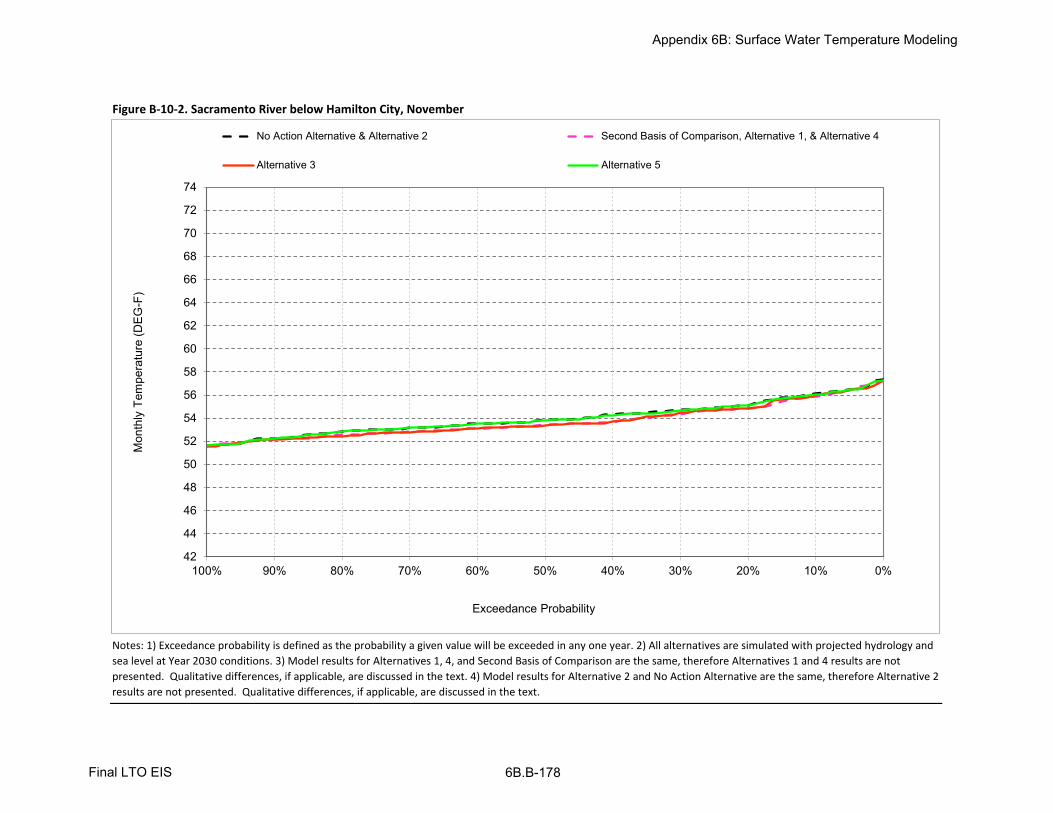
Figure B-10-2. Sacramento River below Hamilton City, November
Notes: 1) Exceedance probability is defined as the probability a given value will be exceeded in any one year. 2) All alternatives are simulated with projected hydrology and
sea level at Year 2030 conditions. 3) Model results for Alternatives 1, 4, and Second Basis of Comparison are the same, therefore Alternatives 1 and 4 results are not
presented. Qualitative differences, if applicable, are discussed in the text. 4) Model results for Alternative 2 and No Action Alternative are the same, therefore Alternative 2
results are not presented. Qualitative differences, if applicable, are discussed in the text.
42
44
46
48
50
52
54
56
58
60
62
64
66
68
70
72
74
0%10%20%30%40%50%60%70%80%90%100%
Exceedance Probability
No Action Alternative & Alternative 2 Second Basis of Comparison, Alternative 1, & Alternative 4
Alternative 3 Alternative 5
Mon
thly
Tem
pera
ture
(DE
G-F
)
Appendix 6B: Surface Water Temperature Modeling
Final LTO EIS 6B.B-178

Figure B-10-3. Sacramento River below Hamilton City, December
Notes: 1) Exceedance probability is defined as the probability a given value will be exceeded in any one year. 2) All alternatives are simulated with projected hydrology and
sea level at Year 2030 conditions. 3) Model results for Alternatives 1, 4, and Second Basis of Comparison are the same, therefore Alternatives 1 and 4 results are not
presented. Qualitative differences, if applicable, are discussed in the text. 4) Model results for Alternative 2 and No Action Alternative are the same, therefore Alternative 2
results are not presented. Qualitative differences, if applicable, are discussed in the text.
42
44
46
48
50
52
54
56
58
60
62
64
66
68
70
72
74
0%10%20%30%40%50%60%70%80%90%100%
Exceedance Probability
No Action Alternative & Alternative 2 Second Basis of Comparison, Alternative 1, & Alternative 4
Alternative 3 Alternative 5
Mon
thly
Tem
pera
ture
(DE
G-F
)
Appendix 6B: Surface Water Temperature Modeling
Final LTO EIS 6B.B-179

Figure B-10-4. Sacramento River below Hamilton City, January
Notes: 1) Exceedance probability is defined as the probability a given value will be exceeded in any one year. 2) All alternatives are simulated with projected hydrology and
sea level at Year 2030 conditions. 3) Model results for Alternatives 1, 4, and Second Basis of Comparison are the same, therefore Alternatives 1 and 4 results are not
presented. Qualitative differences, if applicable, are discussed in the text. 4) Model results for Alternative 2 and No Action Alternative are the same, therefore Alternative 2
results are not presented. Qualitative differences, if applicable, are discussed in the text.
42
44
46
48
50
52
54
56
58
60
62
64
66
68
70
72
74
0%10%20%30%40%50%60%70%80%90%100%
Exceedance Probability
No Action Alternative & Alternative 2 Second Basis of Comparison, Alternative 1, & Alternative 4
Alternative 3 Alternative 5
Mon
thly
Tem
pera
ture
(DE
G-F
)
Appendix 6B: Surface Water Temperature Modeling
Final LTO EIS 6B.B-180

Figure B-10-5. Sacramento River below Hamilton City, February
Notes: 1) Exceedance probability is defined as the probability a given value will be exceeded in any one year. 2) All alternatives are simulated with projected hydrology and
sea level at Year 2030 conditions. 3) Model results for Alternatives 1, 4, and Second Basis of Comparison are the same, therefore Alternatives 1 and 4 results are not
presented. Qualitative differences, if applicable, are discussed in the text. 4) Model results for Alternative 2 and No Action Alternative are the same, therefore Alternative 2
results are not presented. Qualitative differences, if applicable, are discussed in the text.
42
44
46
48
50
52
54
56
58
60
62
64
66
68
70
72
74
0%10%20%30%40%50%60%70%80%90%100%
Exceedance Probability
No Action Alternative & Alternative 2 Second Basis of Comparison, Alternative 1, & Alternative 4
Alternative 3 Alternative 5
Mon
thly
Tem
pera
ture
(DE
G-F
)
Appendix 6B: Surface Water Temperature Modeling
Final LTO EIS 6B.B-181

Figure B-10-6. Sacramento River below Hamilton City, March
Notes: 1) Exceedance probability is defined as the probability a given value will be exceeded in any one year. 2) All alternatives are simulated with projected hydrology and
sea level at Year 2030 conditions. 3) Model results for Alternatives 1, 4, and Second Basis of Comparison are the same, therefore Alternatives 1 and 4 results are not
presented. Qualitative differences, if applicable, are discussed in the text. 4) Model results for Alternative 2 and No Action Alternative are the same, therefore Alternative 2
results are not presented. Qualitative differences, if applicable, are discussed in the text.
42
44
46
48
50
52
54
56
58
60
62
64
66
68
70
72
74
0%10%20%30%40%50%60%70%80%90%100%
Exceedance Probability
No Action Alternative & Alternative 2 Second Basis of Comparison, Alternative 1, & Alternative 4
Alternative 3 Alternative 5
Mon
thly
Tem
pera
ture
(DE
G-F
)
Appendix 6B: Surface Water Temperature Modeling
Final LTO EIS 6B.B-182

Figure B-10-7. Sacramento River below Hamilton City, April
Notes: 1) Exceedance probability is defined as the probability a given value will be exceeded in any one year. 2) All alternatives are simulated with projected hydrology and
sea level at Year 2030 conditions. 3) Model results for Alternatives 1, 4, and Second Basis of Comparison are the same, therefore Alternatives 1 and 4 results are not
presented. Qualitative differences, if applicable, are discussed in the text. 4) Model results for Alternative 2 and No Action Alternative are the same, therefore Alternative 2
results are not presented. Qualitative differences, if applicable, are discussed in the text.
42
44
46
48
50
52
54
56
58
60
62
64
66
68
70
72
74
0%10%20%30%40%50%60%70%80%90%100%
Exceedance Probability
No Action Alternative & Alternative 2 Second Basis of Comparison, Alternative 1, & Alternative 4
Alternative 3 Alternative 5
Mon
thly
Tem
pera
ture
(DE
G-F
)
Appendix 6B: Surface Water Temperature Modeling
Final LTO EIS 6B.B-183

Figure B-10-8. Sacramento River below Hamilton City, May
Notes: 1) Exceedance probability is defined as the probability a given value will be exceeded in any one year. 2) All alternatives are simulated with projected hydrology and
sea level at Year 2030 conditions. 3) Model results for Alternatives 1, 4, and Second Basis of Comparison are the same, therefore Alternatives 1 and 4 results are not
presented. Qualitative differences, if applicable, are discussed in the text. 4) Model results for Alternative 2 and No Action Alternative are the same, therefore Alternative 2
results are not presented. Qualitative differences, if applicable, are discussed in the text.
42
44
46
48
50
52
54
56
58
60
62
64
66
68
70
72
74
0%10%20%30%40%50%60%70%80%90%100%
Exceedance Probability
No Action Alternative & Alternative 2 Second Basis of Comparison, Alternative 1, & Alternative 4
Alternative 3 Alternative 5
Mon
thly
Tem
pera
ture
(DE
G-F
)
Appendix 6B: Surface Water Temperature Modeling
Final LTO EIS 6B.B-184

Figure B-10-9. Sacramento River below Hamilton City, June
Notes: 1) Exceedance probability is defined as the probability a given value will be exceeded in any one year. 2) All alternatives are simulated with projected hydrology and
sea level at Year 2030 conditions. 3) Model results for Alternatives 1, 4, and Second Basis of Comparison are the same, therefore Alternatives 1 and 4 results are not
presented. Qualitative differences, if applicable, are discussed in the text. 4) Model results for Alternative 2 and No Action Alternative are the same, therefore Alternative 2
results are not presented. Qualitative differences, if applicable, are discussed in the text.
42
44
46
48
50
52
54
56
58
60
62
64
66
68
70
72
74
0%10%20%30%40%50%60%70%80%90%100%
Exceedance Probability
No Action Alternative & Alternative 2 Second Basis of Comparison, Alternative 1, & Alternative 4
Alternative 3 Alternative 5
Mon
thly
Tem
pera
ture
(DE
G-F
)
Appendix 6B: Surface Water Temperature Modeling
Final LTO EIS 6B.B-185

Figure B-10-10. Sacramento River below Hamilton City, July
Notes: 1) Exceedance probability is defined as the probability a given value will be exceeded in any one year. 2) All alternatives are simulated with projected hydrology and
sea level at Year 2030 conditions. 3) Model results for Alternatives 1, 4, and Second Basis of Comparison are the same, therefore Alternatives 1 and 4 results are not
presented. Qualitative differences, if applicable, are discussed in the text. 4) Model results for Alternative 2 and No Action Alternative are the same, therefore Alternative 2
results are not presented. Qualitative differences, if applicable, are discussed in the text.
42
44
46
48
50
52
54
56
58
60
62
64
66
68
70
72
74
0%10%20%30%40%50%60%70%80%90%100%
Exceedance Probability
No Action Alternative & Alternative 2 Second Basis of Comparison, Alternative 1, & Alternative 4
Alternative 3 Alternative 5
Mon
thly
Tem
pera
ture
(DE
G-F
)
Appendix 6B: Surface Water Temperature Modeling
Final LTO EIS 6B.B-186

Figure B-10-11. Sacramento River below Hamilton City, August
Notes: 1) Exceedance probability is defined as the probability a given value will be exceeded in any one year. 2) All alternatives are simulated with projected hydrology and
sea level at Year 2030 conditions. 3) Model results for Alternatives 1, 4, and Second Basis of Comparison are the same, therefore Alternatives 1 and 4 results are not
presented. Qualitative differences, if applicable, are discussed in the text. 4) Model results for Alternative 2 and No Action Alternative are the same, therefore Alternative 2
results are not presented. Qualitative differences, if applicable, are discussed in the text.
42
44
46
48
50
52
54
56
58
60
62
64
66
68
70
72
74
0%10%20%30%40%50%60%70%80%90%100%
Exceedance Probability
No Action Alternative & Alternative 2 Second Basis of Comparison, Alternative 1, & Alternative 4
Alternative 3 Alternative 5
Mon
thly
Tem
pera
ture
(DE
G-F
)
Appendix 6B: Surface Water Temperature Modeling
Final LTO EIS 6B.B-187

Figure B-10-12. Sacramento River below Hamilton City, September
Notes: 1) Exceedance probability is defined as the probability a given value will be exceeded in any one year. 2) All alternatives are simulated with projected hydrology and
sea level at Year 2030 conditions. 3) Model results for Alternatives 1, 4, and Second Basis of Comparison are the same, therefore Alternatives 1 and 4 results are not
presented. Qualitative differences, if applicable, are discussed in the text. 4) Model results for Alternative 2 and No Action Alternative are the same, therefore Alternative 2
results are not presented. Qualitative differences, if applicable, are discussed in the text.
42
44
46
48
50
52
54
56
58
60
62
64
66
68
70
72
74
0%10%20%30%40%50%60%70%80%90%100%
Exceedance Probability
No Action Alternative & Alternative 2 Second Basis of Comparison, Alternative 1, & Alternative 4
Alternative 3 Alternative 5
Mon
thly
Tem
pera
ture
(DE
G-F
)
Appendix 6B: Surface Water Temperature Modeling
Final LTO EIS 6B.B-188

Oct Nov Dec Jan Feb Mar Apr May Jun Jul Aug Sep
10% 62 56 50 48 50 55 59 63 65 65 67 6920% 60 55 50 48 50 54 58 63 64 64 66 6730% 60 55 49 47 49 53 58 62 63 64 65 6640% 59 54 49 47 48 53 57 62 63 63 64 6550% 59 54 48 47 48 52 57 61 63 62 64 6360% 58 54 48 46 48 51 56 61 62 62 64 6170% 58 53 48 46 48 51 56 60 62 62 63 6080% 58 53 48 46 47 50 55 60 61 61 63 5990% 57 52 47 46 46 49 54 59 61 61 62 58
Full Simulation Periodb 59 54 49 47 48 52 57 61 63 63 64 63
Wet (32%) 56 52 46 46 47 50 55 60 63 63 64 59Above Normal (16%) 59 54 49 47 48 51 56 61 62 61 63 61Below Normal (13%) 58 54 49 47 49 53 57 61 62 62 63 65
Dry (24%) 59 54 49 47 49 53 58 62 62 63 65 66Critical (15%) 61 55 49 47 50 54 58 62 64 66 68 69
Oct Nov Dec Jan Feb Mar Apr May Jun Jul Aug Sep
10% 62 56 50 48 50 55 59 63 64 65 67 6820% 60 55 49 48 50 54 58 62 64 64 65 6730% 60 54 49 47 49 53 58 62 63 64 65 6640% 59 54 49 47 48 52 57 61 63 63 64 6550% 59 53 48 47 48 52 57 61 62 63 64 6560% 59 53 48 46 48 51 56 61 62 62 63 6470% 58 53 48 46 48 51 55 60 61 62 63 6380% 58 53 48 46 47 50 55 60 61 61 62 6390% 57 52 47 46 46 49 54 59 60 61 61 61
Full Simulation Periodb 59 54 49 47 48 52 56 61 62 63 64 65
Wet (32%) 56 51 47 46 47 50 55 60 63 63 63 63Above Normal (16%) 59 54 48 47 48 51 56 61 62 61 62 63Below Normal (13%) 58 53 48 47 49 53 57 60 61 62 62 64
Dry (24%) 59 54 49 47 49 53 57 61 62 63 65 66Critical (15%) 61 55 49 47 50 54 58 62 64 66 67 69
Oct Nov Dec Jan Feb Mar Apr May Jun Jul Aug Sep
0.1 -0.4 -0.3 0.2 -0.2 0.1 0.0 -0.1 -0.2 -0.5 0.1 0.0 -0.6
0.2 -0.1 -0.3 -0.2 0.1 -0.1 0.0 -0.2 -0.5 -0.1 -0.1 -0.3 -0.2
0.3 0.1 -0.4 -0.2 0.0 0.0 -0.1 0.0 0.0 -0.4 -0.3 -0.3 0.00.4 0.1 -0.7 0.0 0.0 0.0 -0.1 0.0 0.0 -0.3 -0.1 -0.1 0.10.5 0.3 -0.4 -0.1 0.0 0.0 -0.2 -0.1 -0.3 -0.5 0.2 -0.3 1.50.6 0.4 -0.5 0.0 0.0 0.0 -0.1 -0.1 -0.1 -0.5 -0.2 -0.4 3.20.7 0.0 -0.3 0.1 0.0 0.0 -0.1 -0.1 -0.3 -0.6 0.0 -0.4 3.60.8 0.0 -0.3 0.1 0.0 0.0 0.0 0.0 -0.1 -0.6 0.0 -0.6 3.80.9 0.0 -0.1 0.1 0.0 0.1 0.1 0.0 -0.2 -0.5 0.1 -0.4 3.2
Full Simulation Periodb 0.0 -0.3 0.0 0.0 0.0 -0.1 -0.1 -0.2 -0.4 0.0 -0.3 1.6
Wet (32%) 0.1 -0.3 0.1 0.0 0.0 0.0 0.0 -0.1 -0.1 0.1 -0.6 4.2Above Normal (16%) 0.1 -0.3 -0.2 0.0 0.0 -0.1 0.0 -0.2 -0.5 0.1 -0.4 2.9Below Normal (13%) 0.0 -0.4 -0.2 0.0 0.0 -0.3 -0.3 -0.3 -0.6 0.0 -0.6 -0.2
Dry (24%) 0.1 -0.2 -0.1 0.0 0.0 0.0 -0.2 -0.2 -0.6 -0.2 0.2 -0.1
Critical (15%) -0.2 -0.2 0.0 0.1 0.1 0.0 0.0 0.0 -0.6 0.1 -0.2 -0.6
a Exceedance probability is defined as the probability a given value will be exceeded in any one year.
b Based on the 82-year simulation period.
Probability of Exceedancea
Long Term
Water Year Typesc
c As defined by the Sacramento Valley 40-30-30 Index Water Year Hydrologic Classification (SWRCB D-1641, 1999); projected to Year 2030.
Notes: 1) All alternatives are simulated with projected hydrology and sea level at Year 2030 conditions. 2) Model results for Alternatives 1, 4, and Second Basis of Comparison are the same,
therefore Second Basis of Comparison and Alternative 4 results are not presented. Qualitative differences, if applicable, are discussed in the text. 3) Model results for Alternative 2 and No Action
Alternative are the same, therefore Alternative 2 results are not presented. Qualitative differences, if applicable, are discussed in the text.
Probability of Exceedancea
Long Term
Water Year Typesc
Alternative 1 minus No Action Alternative
Statistic
Monthly Temperature (DEG-F)
Long Term
Water Year Typesc
Alternative 1
Statistic
Monthly Temperature (DEG-F)
Table B-10-1. Sacramento River below Hamilton City, Monthly Temperature
No Action Alternative
Statistic
Monthly Temperature (DEG-F)
Probability of Exceedancea
Appendix 6B: Surface Water Temperature Modeling
Final LTO EIS 6B.B-189

Oct Nov Dec Jan Feb Mar Apr May Jun Jul Aug Sep
10% 62 56 50 48 50 55 59 63 65 65 67 6920% 60 55 50 48 50 54 58 63 64 64 66 6730% 60 55 49 47 49 53 58 62 63 64 65 6640% 59 54 49 47 48 53 57 62 63 63 64 6550% 59 54 48 47 48 52 57 61 63 62 64 6360% 58 54 48 46 48 51 56 61 62 62 64 6170% 58 53 48 46 48 51 56 60 62 62 63 6080% 58 53 48 46 47 50 55 60 61 61 63 5990% 57 52 47 46 46 49 54 59 61 61 62 58
Full Simulation Periodb 59 54 49 47 48 52 57 61 63 63 64 63
Wet (32%) 56 52 46 46 47 50 55 60 63 63 64 59Above Normal (16%) 59 54 49 47 48 51 56 61 62 61 63 61Below Normal (13%) 58 54 49 47 49 53 57 61 62 62 63 65
Dry (24%) 59 54 49 47 49 53 58 62 62 63 65 66Critical (15%) 61 55 49 47 50 54 58 62 64 66 68 69
Oct Nov Dec Jan Feb Mar Apr May Jun Jul Aug Sep
10% 61 56 50 48 50 55 59 63 65 65 66 6820% 60 55 49 48 49 54 58 62 64 64 65 6630% 60 54 49 47 49 53 58 62 63 64 65 6540% 59 54 49 47 49 52 57 61 63 63 64 6550% 59 53 48 47 48 52 57 61 62 63 64 6460% 58 53 48 46 48 51 56 60 62 62 63 6470% 58 53 48 46 48 51 56 60 61 62 63 6380% 58 52 48 46 47 50 55 60 61 61 63 6290% 57 52 47 46 46 49 54 59 60 61 62 61
Full Simulation Periodb 59 54 49 47 48 52 56 61 62 63 64 64
Wet (32%) 56 51 47 46 47 50 55 60 63 63 63 63Above Normal (16%) 59 54 48 47 48 51 56 61 62 61 63 63Below Normal (13%) 58 53 48 47 49 53 57 60 61 62 63 63
Dry (24%) 59 54 49 47 49 53 58 61 62 63 65 66Critical (15%) 61 55 49 47 50 54 58 62 64 66 67 69
Oct Nov Dec Jan Feb Mar Apr May Jun Jul Aug Sep
0.1 -0.7 -0.2 0.2 -0.2 0.1 0.0 0.0 -0.1 -0.4 0.1 -0.4 -0.6
0.2 -0.2 -0.3 -0.2 0.1 -0.1 -0.1 -0.2 -0.3 -0.2 -0.1 -0.3 -0.8
0.3 -0.1 -0.2 -0.2 0.0 0.0 -0.1 0.0 0.0 -0.4 -0.2 -0.2 -0.2
0.4 0.1 -0.6 0.0 0.0 0.0 -0.1 0.0 -0.1 -0.3 -0.2 -0.1 0.0
0.5 0.0 -0.5 0.0 0.1 0.0 -0.2 0.0 -0.3 -0.5 0.3 -0.3 1.30.6 0.2 -0.4 0.0 0.0 0.0 0.0 -0.1 -0.2 -0.5 -0.1 -0.2 3.00.7 0.0 -0.4 0.1 0.0 0.0 -0.1 -0.1 -0.3 -0.7 0.0 -0.3 3.10.8 0.2 -0.4 0.1 0.0 0.0 0.0 0.0 -0.1 -0.5 0.0 -0.2 2.80.9 -0.1 -0.1 0.0 0.0 0.1 0.1 0.0 0.0 -0.5 0.3 0.0 3.1
Full Simulation Periodb
0.0 -0.3 0.0 0.0 0.0 0.0 -0.1 -0.2 -0.4 0.0 -0.3 1.3
Wet (32%) 0.1 -0.3 0.1 0.0 0.0 0.0 0.0 -0.1 -0.2 0.0 -0.4 3.9Above Normal (16%) 0.0 -0.3 -0.2 0.0 0.0 -0.1 0.0 -0.3 -0.4 0.1 -0.1 2.9Below Normal (13%) 0.0 -0.4 -0.2 0.0 0.0 -0.3 -0.2 -0.3 -0.5 -0.1 -0.2 -1.4
Dry (24%) -0.1 -0.3 -0.1 0.0 0.0 0.0 -0.1 -0.2 -0.6 -0.2 -0.2 -0.2
Critical (15%) -0.3 -0.2 0.0 0.1 0.0 0.0 0.0 0.0 -0.5 0.3 -0.4 -0.7
a Exceedance probability is defined as the probability a given value will be exceeded in any one year.
b Based on the 82-year simulation period.
Probability of Exceedancea
Long Term
Water Year Typesc
c As defined by the Sacramento Valley 40-30-30 Index Water Year Hydrologic Classification (SWRCB D-1641, 1999); projected to Year 2030.
Notes: 1) All alternatives are simulated with projected hydrology and sea level at Year 2030 conditions. 2) Model results for Alternatives 1, 4, and Second Basis of Comparison are the same,
therefore Alternative 1 and 4 results are not presented. Qualitative differences, if applicable, are discussed in the text. 3) Model results for Alternative 2 and No Action Alternative are the same,
therefore Alternative 2 results are not presented. Qualitative differences, if applicable, are discussed in the text.
Probability of Exceedancea
Long Term
Water Year Typesc
Alternative 3 minus No Action Alternative
Statistic
Monthly Temperature (DEG-F)
Long Term
Water Year Typesc
Alternative 3
Statistic
Monthly Temperature (DEG-F)
Table B-10-2. Sacramento River below Hamilton City, Monthly Temperature
No Action Alternative
Statistic
Monthly Temperature (DEG-F)
Probability of Exceedancea
Appendix 6B: Surface Water Temperature Modeling
Final LTO EIS 6B.B-190

Oct Nov Dec Jan Feb Mar Apr May Jun Jul Aug Sep
10% 62 56 50 48 50 55 59 63 65 65 67 6920% 60 55 50 48 50 54 58 63 64 64 66 6730% 60 55 49 47 49 53 58 62 63 64 65 6640% 59 54 49 47 48 53 57 62 63 63 64 6550% 59 54 48 47 48 52 57 61 63 62 64 6360% 58 54 48 46 48 51 56 61 62 62 64 6170% 58 53 48 46 48 51 56 60 62 62 63 6080% 58 53 48 46 47 50 55 60 61 61 63 5990% 57 52 47 46 46 49 54 59 61 61 62 58
Full Simulation Periodb 59 54 49 47 48 52 57 61 63 63 64 63
Wet (32%) 56 52 46 46 47 50 55 60 63 63 64 59Above Normal (16%) 59 54 49 47 48 51 56 61 62 61 63 61Below Normal (13%) 58 54 49 47 49 53 57 61 62 62 63 65
Dry (24%) 59 54 49 47 49 53 58 62 62 63 65 66Critical (15%) 61 55 49 47 50 54 58 62 64 66 68 69
Oct Nov Dec Jan Feb Mar Apr May Jun Jul Aug Sep
10% 62 56 50 48 50 55 59 63 65 65 67 6820% 60 55 50 48 50 54 58 63 64 64 66 6730% 60 55 49 47 49 53 58 62 63 64 65 6640% 59 54 49 47 48 53 57 62 63 63 64 6550% 58 54 48 47 48 52 57 61 63 62 64 6360% 58 53 48 46 48 51 56 61 62 62 64 6170% 58 53 48 46 48 51 56 60 62 62 63 6080% 58 53 48 46 47 50 55 60 61 61 63 5990% 57 52 47 46 46 49 54 59 61 61 62 58
Full Simulation Periodb 59 54 49 47 48 52 57 61 63 63 64 63
Wet (32%) 56 52 46 46 47 50 55 60 63 63 64 59Above Normal (16%) 59 54 49 47 48 51 56 61 62 61 63 61Below Normal (13%) 58 54 49 47 49 53 57 61 62 62 63 64
Dry (24%) 59 54 49 47 49 53 58 62 62 63 65 66Critical (15%) 61 55 49 47 50 54 58 63 64 65 67 69
Oct Nov Dec Jan Feb Mar Apr May Jun Jul Aug Sep
0.1 0.0 -0.1 0.0 0.0 0.0 0.0 0.1 0.0 0.1 -0.1 0.0 -0.1
0.2 0.0 0.0 0.0 0.1 0.0 0.0 -0.2 0.2 0.0 0.0 -0.2 -0.2
0.3 0.0 -0.1 -0.1 0.0 0.0 0.0 0.0 0.0 0.0 -0.1 -0.1 0.00.4 0.0 -0.1 0.0 0.0 0.0 0.0 0.1 0.1 0.0 -0.1 0.0 -0.3
0.5 -0.2 0.0 0.0 0.0 0.0 0.0 0.1 0.1 0.0 -0.1 -0.2 -0.1
0.6 0.0 0.0 0.0 0.0 0.0 0.0 0.1 0.1 0.1 -0.1 0.0 -0.1
0.7 -0.2 0.0 0.0 0.0 0.0 0.0 0.0 0.1 0.0 -0.1 -0.2 0.00.8 0.1 0.0 0.0 0.0 0.0 0.0 0.0 0.2 0.0 0.0 0.0 0.00.9 0.0 0.0 0.0 0.0 0.0 0.0 0.0 0.0 0.0 0.0 0.0 0.0
Full Simulation Periodb
0.0 0.0 0.0 0.0 0.0 0.0 0.0 0.1 0.0 -0.1 -0.1 -0.1
Wet (32%) 0.0 0.0 0.0 0.0 0.0 0.0 0.0 0.0 0.0 0.0 0.0 0.0Above Normal (16%) 0.0 -0.1 0.0 0.0 0.0 0.0 0.0 0.1 0.0 0.0 0.0 0.1Below Normal (13%) 0.0 0.0 0.0 0.0 0.0 0.0 0.0 0.1 0.0 0.0 0.2 -0.2
Dry (24%) 0.0 0.0 0.0 0.0 0.0 0.0 0.1 0.3 0.0 -0.1 -0.3 -0.2
Critical (15%) 0.0 0.0 0.0 0.0 0.0 0.0 0.1 0.2 0.2 -0.2 -0.3 -0.1
a Exceedance probability is defined as the probability a given value will be exceeded in any one year.
b Based on the 82-year simulation period.
Probability of Exceedancea
Long Term
Water Year Typesc
c As defined by the Sacramento Valley 40-30-30 Index Water Year Hydrologic Classification (SWRCB D-1641, 1999); projected to Year 2030.
Notes: 1) All alternatives are simulated with projected hydrology and sea level at Year 2030 conditions. 2) Model results for Alternatives 1, 4, and Second Basis of Comparison are the same,
therefore Alternative 1 and 4 results are not presented. Qualitative differences, if applicable, are discussed in the text. 3) Model results for Alternative 2 and No Action Alternative are the same,
therefore Alternative 2 results are not presented. Qualitative differences, if applicable, are discussed in the text.
Probability of Exceedancea
Long Term
Water Year Typesc
Alternative 5 minus No Action Alternative
Statistic
Monthly Temperature (DEG-F)
Long Term
Water Year Typesc
Alternative 5
Statistic
Monthly Temperature (DEG-F)
Table B-10-3. Sacramento River below Hamilton City, Monthly Temperature
No Action Alternative
Statistic
Monthly Temperature (DEG-F)
Probability of Exceedancea
Appendix 6B: Surface Water Temperature Modeling
Final LTO EIS 6B.B-191

Oct Nov Dec Jan Feb Mar Apr May Jun Jul Aug Sep
10% 62 56 50 48 50 55 59 63 64 65 67 6820% 60 55 49 48 50 54 58 62 64 64 65 6730% 60 54 49 47 49 53 58 62 63 64 65 6640% 59 54 49 47 48 52 57 61 63 63 64 6550% 59 53 48 47 48 52 57 61 62 63 64 6560% 59 53 48 46 48 51 56 61 62 62 63 6470% 58 53 48 46 48 51 55 60 61 62 63 6380% 58 53 48 46 47 50 55 60 61 61 62 6390% 57 52 47 46 46 49 54 59 60 61 61 61
Full Simulation Periodb 59 54 49 47 48 52 56 61 62 63 64 65
Wet (32%) 56 51 47 46 47 50 55 60 63 63 63 63Above Normal (16%) 59 54 48 47 48 51 56 61 62 61 62 63Below Normal (13%) 58 53 48 47 49 53 57 60 61 62 62 64
Dry (24%) 59 54 49 47 49 53 57 61 62 63 65 66Critical (15%) 61 55 49 47 50 54 58 62 64 66 67 69
Oct Nov Dec Jan Feb Mar Apr May Jun Jul Aug Sep
10% 62 56 50 48 50 55 59 63 65 65 67 6920% 60 55 50 48 50 54 58 63 64 64 66 6730% 60 55 49 47 49 53 58 62 63 64 65 6640% 59 54 49 47 48 53 57 62 63 63 64 6550% 59 54 48 47 48 52 57 61 63 62 64 6360% 58 54 48 46 48 51 56 61 62 62 64 6170% 58 53 48 46 48 51 56 60 62 62 63 6080% 58 53 48 46 47 50 55 60 61 61 63 5990% 57 52 47 46 46 49 54 59 61 61 62 58
Full Simulation Periodb 59 54 49 47 48 52 57 61 63 63 64 63
Wet (32%) 56 52 46 46 47 50 55 60 63 63 64 59Above Normal (16%) 59 54 49 47 48 51 56 61 62 61 63 61Below Normal (13%) 58 54 49 47 49 53 57 61 62 62 63 65
Dry (24%) 59 54 49 47 49 53 58 62 62 63 65 66Critical (15%) 61 55 49 47 50 54 58 62 64 66 68 69
Oct Nov Dec Jan Feb Mar Apr May Jun Jul Aug Sep
0.1 0.4 0.3 -0.2 0.2 -0.1 0.0 0.1 0.2 0.5 -0.1 0.0 0.60.2 0.1 0.3 0.2 -0.1 0.1 0.0 0.2 0.5 0.1 0.1 0.3 0.20.3 -0.1 0.4 0.2 0.0 0.0 0.1 0.0 0.0 0.4 0.3 0.3 0.0
0.4 -0.1 0.7 0.0 0.0 0.0 0.1 0.0 0.0 0.3 0.1 0.1 -0.1
0.5 -0.3 0.4 0.1 0.0 0.0 0.2 0.1 0.3 0.5 -0.2 0.3 -1.5
0.6 -0.4 0.5 0.0 0.0 0.0 0.1 0.1 0.1 0.5 0.2 0.4 -3.2
0.7 0.0 0.3 -0.1 0.0 0.0 0.1 0.1 0.3 0.6 0.0 0.4 -3.6
0.8 0.0 0.3 -0.1 0.0 0.0 0.0 0.0 0.1 0.6 0.0 0.6 -3.8
0.9 0.0 0.1 -0.1 0.0 -0.1 -0.1 0.0 0.2 0.5 -0.1 0.4 -3.2
Full Simulation Periodb
0.0 0.3 0.0 0.0 0.0 0.1 0.1 0.2 0.4 0.0 0.3 -1.6
Wet (32%) -0.1 0.3 -0.1 0.0 0.0 0.0 0.0 0.1 0.1 -0.1 0.6 -4.2
Above Normal (16%) -0.1 0.3 0.2 0.0 0.0 0.1 0.0 0.2 0.5 -0.1 0.4 -2.9
Below Normal (13%) 0.0 0.4 0.2 0.0 0.0 0.3 0.3 0.3 0.6 0.0 0.6 0.2Dry (24%) -0.1 0.2 0.1 0.0 0.0 0.0 0.2 0.2 0.6 0.2 -0.2 0.1
Critical (15%) 0.2 0.2 0.0 -0.1 -0.1 0.0 0.0 0.0 0.6 -0.1 0.2 0.6
a Exceedance probability is defined as the probability a given value will be exceeded in any one year.
b Based on the 82-year simulation period.
Probability of Exceedancea
Long Term
Water Year Typesc
c As defined by the Sacramento Valley 40-30-30 Index Water Year Hydrologic Classification (SWRCB D-1641, 1999); projected to Year 2030.
Notes: 1) All alternatives are simulated with projected hydrology and sea level at Year 2030 conditions. 2) Model results for Alternatives 1, 4, and Second Basis of Comparison are the same,
therefore Alternative 1 and 4 results are not presented. Qualitative differences, if applicable, are discussed in the text. 3) Model results for Alternative 2 and No Action Alternative are the same,
therefore Alternative 2 results are not presented. Qualitative differences, if applicable, are discussed in the text.
Probability of Exceedancea
Long Term
Water Year Typesc
No Action Alternative minus Second Basis of Comparison
Statistic
Monthly Temperature (DEG-F)
Long Term
Water Year Typesc
No Action Alternative
Statistic
Monthly Temperature (DEG-F)
Table B-10-4. Sacramento River below Hamilton City, Monthly Temperature
Second Basis of Comparison
Statistic
Monthly Temperature (DEG-F)
Probability of Exceedancea
Appendix 6B: Surface Water Temperature Modeling
Final LTO EIS 6B.B-192

Oct Nov Dec Jan Feb Mar Apr May Jun Jul Aug Sep
10% 62 56 50 48 50 55 59 63 64 65 67 6820% 60 55 49 48 50 54 58 62 64 64 65 6730% 60 54 49 47 49 53 58 62 63 64 65 6640% 59 54 49 47 48 52 57 61 63 63 64 6550% 59 53 48 47 48 52 57 61 62 63 64 6560% 59 53 48 46 48 51 56 61 62 62 63 6470% 58 53 48 46 48 51 55 60 61 62 63 6380% 58 53 48 46 47 50 55 60 61 61 62 6390% 57 52 47 46 46 49 54 59 60 61 61 61
Full Simulation Periodb 59 54 49 47 48 52 56 61 62 63 64 65
Wet (32%) 56 51 47 46 47 50 55 60 63 63 63 63Above Normal (16%) 59 54 48 47 48 51 56 61 62 61 62 63Below Normal (13%) 58 53 48 47 49 53 57 60 61 62 62 64
Dry (24%) 59 54 49 47 49 53 57 61 62 63 65 66Critical (15%) 61 55 49 47 50 54 58 62 64 66 67 69
Oct Nov Dec Jan Feb Mar Apr May Jun Jul Aug Sep
10% 61 56 50 48 50 55 59 63 65 65 66 6820% 60 55 49 48 49 54 58 62 64 64 65 6630% 60 54 49 47 49 53 58 62 63 64 65 6540% 59 54 49 47 49 52 57 61 63 63 64 6550% 59 53 48 47 48 52 57 61 62 63 64 6460% 58 53 48 46 48 51 56 60 62 62 63 6470% 58 53 48 46 48 51 56 60 61 62 63 6380% 58 52 48 46 47 50 55 60 61 61 63 6290% 57 52 47 46 46 49 54 59 60 61 62 61
Full Simulation Periodb 59 54 49 47 48 52 56 61 62 63 64 64
Wet (32%) 56 51 47 46 47 50 55 60 63 63 63 63Above Normal (16%) 59 54 48 47 48 51 56 61 62 61 63 63Below Normal (13%) 58 53 48 47 49 53 57 60 61 62 63 63
Dry (24%) 59 54 49 47 49 53 58 61 62 63 65 66Critical (15%) 61 55 49 47 50 54 58 62 64 66 67 69
Oct Nov Dec Jan Feb Mar Apr May Jun Jul Aug Sep
0.1 -0.3 0.1 0.0 0.0 0.0 0.0 0.0 0.1 0.1 0.0 -0.5 0.0
0.2 -0.2 0.0 0.0 0.0 -0.1 0.0 0.0 0.2 0.0 0.0 0.0 -0.6
0.3 -0.1 0.2 0.0 0.0 0.0 0.0 0.0 0.0 0.0 0.1 0.1 -0.2
0.4 0.0 0.0 0.0 0.0 0.0 0.0 0.0 -0.1 0.0 -0.1 0.0 -0.2
0.5 -0.2 -0.1 0.1 0.0 0.1 0.0 0.1 0.0 0.1 0.1 0.0 -0.2
0.6 -0.2 0.0 0.0 0.0 0.0 0.0 0.0 -0.1 0.0 0.1 0.2 -0.2
0.7 0.0 0.0 0.0 0.0 0.0 0.0 0.1 0.0 0.0 0.0 0.1 -0.6
0.8 0.2 -0.1 0.0 0.0 0.0 0.0 0.0 -0.1 0.1 0.0 0.4 -1.0
0.9 -0.1 0.0 -0.1 0.0 0.0 0.0 0.0 0.2 0.1 0.1 0.4 -0.1
Full Simulation Periodb
-0.1 0.0 0.0 0.0 0.0 0.0 0.0 0.0 0.0 0.0 0.1 -0.3
Wet (32%) 0.0 0.0 0.0 0.0 0.0 0.0 0.0 0.0 -0.1 -0.1 0.3 -0.3
Above Normal (16%) -0.1 0.0 0.0 0.0 0.0 0.0 0.0 -0.1 0.1 0.0 0.3 0.0Below Normal (13%) 0.0 0.0 0.0 0.0 0.0 0.0 0.1 0.0 0.2 0.0 0.4 -1.2
Dry (24%) -0.2 -0.1 0.0 0.0 0.0 0.0 0.1 0.0 0.0 0.0 -0.4 -0.1
Critical (15%) -0.1 0.0 0.0 0.0 -0.1 0.0 0.1 0.0 0.1 0.2 -0.2 -0.1
a Exceedance probability is defined as the probability a given value will be exceeded in any one year.
b Based on the 82-year simulation period.
Probability of Exceedancea
Long Term
Water Year Typesc
c As defined by the Sacramento Valley 40-30-30 Index Water Year Hydrologic Classification (SWRCB D-1641, 1999); projected to Year 2030.
Notes: 1) All alternatives are simulated with projected hydrology and sea level at Year 2030 conditions. 2) Model results for Alternatives 1, 4, and Second Basis of Comparison are the same,
therefore Alternative 1 and 4 results are not presented. Qualitative differences, if applicable, are discussed in the text. 3) Model results for Alternative 2 and No Action Alternative are the same,
therefore Alternative 2 results are not presented. Qualitative differences, if applicable, are discussed in the text.
Probability of Exceedancea
Long Term
Water Year Typesc
Alternative 3 minus Second Basis of Comparison
Statistic
Monthly Temperature (DEG-F)
Long Term
Water Year Typesc
Alternative 3
Statistic
Monthly Temperature (DEG-F)
Table B-10-5. Sacramento River below Hamilton City, Monthly Temperature
Second Basis of Comparison
Statistic
Monthly Temperature (DEG-F)
Probability of Exceedancea
Appendix 6B: Surface Water Temperature Modeling
Final LTO EIS 6B.B-193

Oct Nov Dec Jan Feb Mar Apr May Jun Jul Aug Sep
10% 62 56 50 48 50 55 59 63 64 65 67 6820% 60 55 49 48 50 54 58 62 64 64 65 6730% 60 54 49 47 49 53 58 62 63 64 65 6640% 59 54 49 47 48 52 57 61 63 63 64 6550% 59 53 48 47 48 52 57 61 62 63 64 6560% 59 53 48 46 48 51 56 61 62 62 63 6470% 58 53 48 46 48 51 55 60 61 62 63 6380% 58 53 48 46 47 50 55 60 61 61 62 6390% 57 52 47 46 46 49 54 59 60 61 61 61
Full Simulation Periodb 59 54 49 47 48 52 56 61 62 63 64 65
Wet (32%) 56 51 47 46 47 50 55 60 63 63 63 63Above Normal (16%) 59 54 48 47 48 51 56 61 62 61 62 63Below Normal (13%) 58 53 48 47 49 53 57 60 61 62 62 64
Dry (24%) 59 54 49 47 49 53 57 61 62 63 65 66Critical (15%) 61 55 49 47 50 54 58 62 64 66 67 69
Oct Nov Dec Jan Feb Mar Apr May Jun Jul Aug Sep
10% 62 56 50 48 50 55 59 63 65 65 67 6820% 60 55 50 48 50 54 58 63 64 64 66 6730% 60 55 49 47 49 53 58 62 63 64 65 6640% 59 54 49 47 48 53 57 62 63 63 64 6550% 58 54 48 47 48 52 57 61 63 62 64 6360% 58 53 48 46 48 51 56 61 62 62 64 6170% 58 53 48 46 48 51 56 60 62 62 63 6080% 58 53 48 46 47 50 55 60 61 61 63 5990% 57 52 47 46 46 49 54 59 61 61 62 58
Full Simulation Periodb 59 54 49 47 48 52 57 61 63 63 64 63
Wet (32%) 56 52 46 46 47 50 55 60 63 63 64 59Above Normal (16%) 59 54 49 47 48 51 56 61 62 61 63 61Below Normal (13%) 58 54 49 47 49 53 57 61 62 62 63 64
Dry (24%) 59 54 49 47 49 53 58 62 62 63 65 66Critical (15%) 61 55 49 47 50 54 58 63 64 65 67 69
Oct Nov Dec Jan Feb Mar Apr May Jun Jul Aug Sep
0.1 0.4 0.2 -0.2 0.2 0.0 0.0 0.1 0.2 0.5 -0.2 -0.1 0.50.2 0.0 0.3 0.2 -0.1 0.1 0.0 0.0 0.6 0.1 0.1 0.1 0.10.3 -0.1 0.3 0.1 0.0 0.0 0.1 0.0 0.1 0.4 0.1 0.2 0.00.4 -0.2 0.6 0.0 0.0 0.0 0.1 0.1 0.2 0.3 0.0 0.0 -0.5
0.5 -0.5 0.4 0.1 0.0 0.0 0.2 0.2 0.3 0.5 -0.3 0.1 -1.6
0.6 -0.3 0.4 0.0 0.0 0.0 0.1 0.2 0.3 0.6 0.2 0.4 -3.3
0.7 -0.2 0.4 -0.1 0.0 0.0 0.1 0.2 0.4 0.7 -0.1 0.2 -3.6
0.8 0.0 0.2 -0.1 0.0 0.0 0.0 0.0 0.3 0.6 0.0 0.6 -3.8
0.9 -0.1 0.1 -0.1 0.0 -0.1 -0.1 0.0 0.2 0.5 -0.1 0.4 -3.2
Full Simulation Periodb
0.0 0.3 0.0 0.0 0.0 0.0 0.1 0.3 0.5 -0.1 0.2 -1.7
Wet (32%) -0.1 0.3 -0.2 0.0 0.0 0.0 0.0 0.1 0.1 -0.1 0.6 -4.1
Above Normal (16%) -0.1 0.3 0.2 0.0 0.0 0.1 0.0 0.3 0.6 -0.1 0.5 -2.8
Below Normal (13%) 0.0 0.4 0.2 0.0 0.0 0.3 0.2 0.4 0.7 0.0 0.8 0.0Dry (24%) 0.0 0.2 0.1 0.0 0.0 0.0 0.2 0.5 0.6 0.1 -0.5 -0.1
Critical (15%) 0.1 0.2 0.0 -0.1 -0.1 0.0 0.2 0.3 0.8 -0.3 -0.2 0.5
a Exceedance probability is defined as the probability a given value will be exceeded in any one year.
b Based on the 82-year simulation period.
Probability of Exceedancea
Long Term
Water Year Typesc
c As defined by the Sacramento Valley 40-30-30 Index Water Year Hydrologic Classification (SWRCB D-1641, 1999); projected to Year 2030.
Notes: 1) All alternatives are simulated with projected hydrology and sea level at Year 2030 conditions. 2) Model results for Alternatives 1, 4, and Second Basis of Comparison are the same,
therefore Alternative 1 and 4 results are not presented. Qualitative differences, if applicable, are discussed in the text. 3) Model results for Alternative 2 and No Action Alternative are the same,
therefore Alternative 2 results are not presented. Qualitative differences, if applicable, are discussed in the text.
Probability of Exceedancea
Long Term
Water Year Typesc
Alternative 5 minus Second Basis of Comparison
Statistic
Monthly Temperature (DEG-F)
Long Term
Water Year Typesc
Alternative 5
Statistic
Monthly Temperature (DEG-F)
Table B-10-6. Sacramento River below Hamilton City, Monthly Temperature
Second Basis of Comparison
Statistic
Monthly Temperature (DEG-F)
Probability of Exceedancea
Appendix 6B: Surface Water Temperature Modeling
Final LTO EIS 6B.B-194

B.11. Sacramento River at Knights Landing Temperature
Appendix 6B: Surface Water Temperature Modeling
Final LTO EIS 6B.B-195

Figure B-11-1. Sacramento River at Knights Landing, October
Notes: 1) Exceedance probability is defined as the probability a given value will be exceeded in any one year. 2) All alternatives are simulated with projected hydrology and
sea level at Year 2030 conditions. 3) Model results for Alternatives 1, 4, and Second Basis of Comparison are the same, therefore Alternatives 1 and 4 results are not
presented. Qualitative differences, if applicable, are discussed in the text. 4) Model results for Alternative 2 and No Action Alternative are the same, therefore Alternative 2
results are not presented. Qualitative differences, if applicable, are discussed in the text.
4244464850525456586062646668707274767880
0%10%20%30%40%50%60%70%80%90%100%
Exceedance Probability
No Action Alternative & Alternative 2 Second Basis of Comparison, Alternative 1, & Alternative 4
Alternative 3 Alternative 5
Mon
thly
Tem
pera
ture
(DE
G-F
)
Appendix 6B: Surface Water Temperature Modeling
Final LTO EIS 6B.B-196

Figure B-11-2. Sacramento River at Knights Landing, November
Notes: 1) Exceedance probability is defined as the probability a given value will be exceeded in any one year. 2) All alternatives are simulated with projected hydrology and
sea level at Year 2030 conditions. 3) Model results for Alternatives 1, 4, and Second Basis of Comparison are the same, therefore Alternatives 1 and 4 results are not
presented. Qualitative differences, if applicable, are discussed in the text. 4) Model results for Alternative 2 and No Action Alternative are the same, therefore Alternative 2
results are not presented. Qualitative differences, if applicable, are discussed in the text.
4244464850525456586062646668707274767880
0%10%20%30%40%50%60%70%80%90%100%
Exceedance Probability
No Action Alternative & Alternative 2 Second Basis of Comparison, Alternative 1, & Alternative 4
Alternative 3 Alternative 5
Mon
thly
Tem
pera
ture
(DE
G-F
)
Appendix 6B: Surface Water Temperature Modeling
Final LTO EIS 6B.B-197

Figure B-11-3. Sacramento River at Knights Landing, December
Notes: 1) Exceedance probability is defined as the probability a given value will be exceeded in any one year. 2) All alternatives are simulated with projected hydrology and
sea level at Year 2030 conditions. 3) Model results for Alternatives 1, 4, and Second Basis of Comparison are the same, therefore Alternatives 1 and 4 results are not
presented. Qualitative differences, if applicable, are discussed in the text. 4) Model results for Alternative 2 and No Action Alternative are the same, therefore Alternative 2
results are not presented. Qualitative differences, if applicable, are discussed in the text.
4244464850525456586062646668707274767880
0%10%20%30%40%50%60%70%80%90%100%
Exceedance Probability
No Action Alternative & Alternative 2 Second Basis of Comparison, Alternative 1, & Alternative 4
Alternative 3 Alternative 5
Mon
thly
Tem
pera
ture
(DE
G-F
)
Appendix 6B: Surface Water Temperature Modeling
Final LTO EIS 6B.B-198
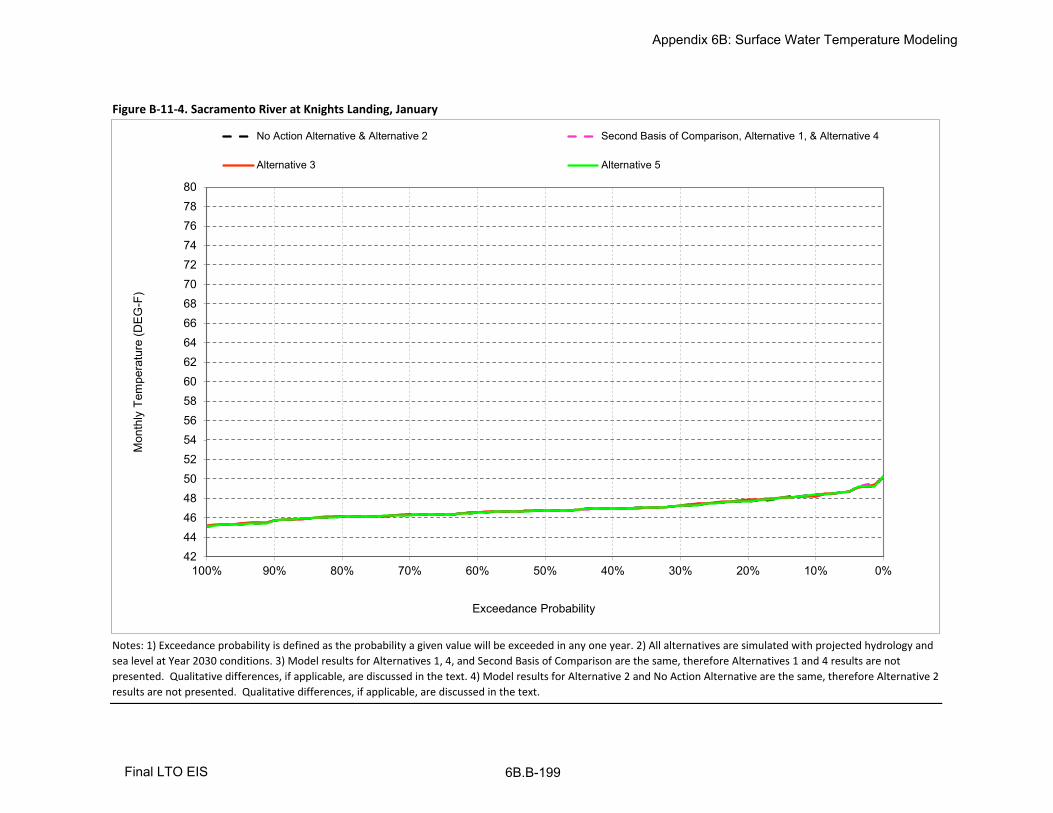
Figure B-11-4. Sacramento River at Knights Landing, January
Notes: 1) Exceedance probability is defined as the probability a given value will be exceeded in any one year. 2) All alternatives are simulated with projected hydrology and
sea level at Year 2030 conditions. 3) Model results for Alternatives 1, 4, and Second Basis of Comparison are the same, therefore Alternatives 1 and 4 results are not
presented. Qualitative differences, if applicable, are discussed in the text. 4) Model results for Alternative 2 and No Action Alternative are the same, therefore Alternative 2
results are not presented. Qualitative differences, if applicable, are discussed in the text.
4244464850525456586062646668707274767880
0%10%20%30%40%50%60%70%80%90%100%
Exceedance Probability
No Action Alternative & Alternative 2 Second Basis of Comparison, Alternative 1, & Alternative 4
Alternative 3 Alternative 5
Mon
thly
Tem
pera
ture
(DE
G-F
)
Appendix 6B: Surface Water Temperature Modeling
Final LTO EIS 6B.B-199

Figure B-11-5. Sacramento River at Knights Landing, February
Notes: 1) Exceedance probability is defined as the probability a given value will be exceeded in any one year. 2) All alternatives are simulated with projected hydrology and
sea level at Year 2030 conditions. 3) Model results for Alternatives 1, 4, and Second Basis of Comparison are the same, therefore Alternatives 1 and 4 results are not
presented. Qualitative differences, if applicable, are discussed in the text. 4) Model results for Alternative 2 and No Action Alternative are the same, therefore Alternative 2
results are not presented. Qualitative differences, if applicable, are discussed in the text.
4244464850525456586062646668707274767880
0%10%20%30%40%50%60%70%80%90%100%
Exceedance Probability
No Action Alternative & Alternative 2 Second Basis of Comparison, Alternative 1, & Alternative 4
Alternative 3 Alternative 5
Mon
thly
Tem
pera
ture
(DE
G-F
)
Appendix 6B: Surface Water Temperature Modeling
Final LTO EIS 6B.B-200

Figure B-11-6. Sacramento River at Knights Landing, March
Notes: 1) Exceedance probability is defined as the probability a given value will be exceeded in any one year. 2) All alternatives are simulated with projected hydrology and
sea level at Year 2030 conditions. 3) Model results for Alternatives 1, 4, and Second Basis of Comparison are the same, therefore Alternatives 1 and 4 results are not
presented. Qualitative differences, if applicable, are discussed in the text. 4) Model results for Alternative 2 and No Action Alternative are the same, therefore Alternative 2
results are not presented. Qualitative differences, if applicable, are discussed in the text.
4244464850525456586062646668707274767880
0%10%20%30%40%50%60%70%80%90%100%
Exceedance Probability
No Action Alternative & Alternative 2 Second Basis of Comparison, Alternative 1, & Alternative 4
Alternative 3 Alternative 5
Mon
thly
Tem
pera
ture
(DE
G-F
)
Appendix 6B: Surface Water Temperature Modeling
Final LTO EIS 6B.B-201

Figure B-11-7. Sacramento River at Knights Landing, April
Notes: 1) Exceedance probability is defined as the probability a given value will be exceeded in any one year. 2) All alternatives are simulated with projected hydrology and
sea level at Year 2030 conditions. 3) Model results for Alternatives 1, 4, and Second Basis of Comparison are the same, therefore Alternatives 1 and 4 results are not
presented. Qualitative differences, if applicable, are discussed in the text. 4) Model results for Alternative 2 and No Action Alternative are the same, therefore Alternative 2
results are not presented. Qualitative differences, if applicable, are discussed in the text.
4244464850525456586062646668707274767880
0%10%20%30%40%50%60%70%80%90%100%
Exceedance Probability
No Action Alternative & Alternative 2 Second Basis of Comparison, Alternative 1, & Alternative 4
Alternative 3 Alternative 5
Mon
thly
Tem
pera
ture
(DE
G-F
)
Appendix 6B: Surface Water Temperature Modeling
Final LTO EIS 6B.B-202

Figure B-11-8. Sacramento River at Knights Landing, May
Notes: 1) Exceedance probability is defined as the probability a given value will be exceeded in any one year. 2) All alternatives are simulated with projected hydrology and
sea level at Year 2030 conditions. 3) Model results for Alternatives 1, 4, and Second Basis of Comparison are the same, therefore Alternatives 1 and 4 results are not
presented. Qualitative differences, if applicable, are discussed in the text. 4) Model results for Alternative 2 and No Action Alternative are the same, therefore Alternative 2
results are not presented. Qualitative differences, if applicable, are discussed in the text.
4244464850525456586062646668707274767880
0%10%20%30%40%50%60%70%80%90%100%
Exceedance Probability
No Action Alternative & Alternative 2 Second Basis of Comparison, Alternative 1, & Alternative 4
Alternative 3 Alternative 5
Mon
thly
Tem
pera
ture
(DE
G-F
)
Appendix 6B: Surface Water Temperature Modeling
Final LTO EIS 6B.B-203

Figure B-11-9. Sacramento River at Knights Landing, June
Notes: 1) Exceedance probability is defined as the probability a given value will be exceeded in any one year. 2) All alternatives are simulated with projected hydrology and
sea level at Year 2030 conditions. 3) Model results for Alternatives 1, 4, and Second Basis of Comparison are the same, therefore Alternatives 1 and 4 results are not
presented. Qualitative differences, if applicable, are discussed in the text. 4) Model results for Alternative 2 and No Action Alternative are the same, therefore Alternative 2
results are not presented. Qualitative differences, if applicable, are discussed in the text.
4244464850525456586062646668707274767880
0%10%20%30%40%50%60%70%80%90%100%
Exceedance Probability
No Action Alternative & Alternative 2 Second Basis of Comparison, Alternative 1, & Alternative 4
Alternative 3 Alternative 5
Mon
thly
Tem
pera
ture
(DE
G-F
)
Appendix 6B: Surface Water Temperature Modeling
Final LTO EIS 6B.B-204

Figure B-11-10. Sacramento River at Knights Landing, July
Notes: 1) Exceedance probability is defined as the probability a given value will be exceeded in any one year. 2) All alternatives are simulated with projected hydrology and
sea level at Year 2030 conditions. 3) Model results for Alternatives 1, 4, and Second Basis of Comparison are the same, therefore Alternatives 1 and 4 results are not
presented. Qualitative differences, if applicable, are discussed in the text. 4) Model results for Alternative 2 and No Action Alternative are the same, therefore Alternative 2
results are not presented. Qualitative differences, if applicable, are discussed in the text.
4244464850525456586062646668707274767880
0%10%20%30%40%50%60%70%80%90%100%
Exceedance Probability
No Action Alternative & Alternative 2 Second Basis of Comparison, Alternative 1, & Alternative 4
Alternative 3 Alternative 5
Mon
thly
Tem
pera
ture
(DE
G-F
)
Appendix 6B: Surface Water Temperature Modeling
Final LTO EIS 6B.B-205

Figure B-11-11. Sacramento River at Knights Landing, August
Notes: 1) Exceedance probability is defined as the probability a given value will be exceeded in any one year. 2) All alternatives are simulated with projected hydrology and
sea level at Year 2030 conditions. 3) Model results for Alternatives 1, 4, and Second Basis of Comparison are the same, therefore Alternatives 1 and 4 results are not
presented. Qualitative differences, if applicable, are discussed in the text. 4) Model results for Alternative 2 and No Action Alternative are the same, therefore Alternative 2
results are not presented. Qualitative differences, if applicable, are discussed in the text.
4244464850525456586062646668707274767880
0%10%20%30%40%50%60%70%80%90%100%
Exceedance Probability
No Action Alternative & Alternative 2 Second Basis of Comparison, Alternative 1, & Alternative 4
Alternative 3 Alternative 5
Mon
thly
Tem
pera
ture
(DE
G-F
)
Appendix 6B: Surface Water Temperature Modeling
Final LTO EIS 6B.B-206

Figure B-11-12. Sacramento River at Knights Landing, September
Notes: 1) Exceedance probability is defined as the probability a given value will be exceeded in any one year. 2) All alternatives are simulated with projected hydrology and
sea level at Year 2030 conditions. 3) Model results for Alternatives 1, 4, and Second Basis of Comparison are the same, therefore Alternatives 1 and 4 results are not
presented. Qualitative differences, if applicable, are discussed in the text. 4) Model results for Alternative 2 and No Action Alternative are the same, therefore Alternative 2
results are not presented. Qualitative differences, if applicable, are discussed in the text.
4244464850525456586062646668707274767880
0%10%20%30%40%50%60%70%80%90%100%
Exceedance Probability
No Action Alternative & Alternative 2 Second Basis of Comparison, Alternative 1, & Alternative 4
Alternative 3 Alternative 5
Mon
thly
Tem
pera
ture
(DE
G-F
)
Appendix 6B: Surface Water Temperature Modeling
Final LTO EIS 6B.B-207

Oct Nov Dec Jan Feb Mar Apr May Jun Jul Aug Sep
10% 65 58 50 48 51 57 63 69 73 74 75 7420% 65 57 50 48 50 56 62 69 72 73 74 7330% 64 56 49 47 50 55 62 68 72 73 74 7240% 63 55 49 47 49 54 61 68 71 72 73 7150% 63 55 48 47 49 54 61 67 71 71 73 6960% 62 55 48 47 48 53 60 67 70 71 72 6770% 61 54 48 46 48 52 59 66 70 70 72 6680% 61 54 48 46 48 51 57 65 69 70 71 6590% 60 53 47 46 47 51 56 63 69 69 70 63
Full Simulation Periodb 63 55 49 47 49 54 60 67 71 72 73 69
Wet (32%) 60 53 46 46 48 52 57 65 70 72 72 65Above Normal (16%) 63 55 49 47 48 53 59 67 71 70 72 67Below Normal (13%) 62 54 48 47 49 55 62 67 70 71 71 71
Dry (24%) 63 55 49 47 50 55 61 68 71 72 73 72Critical (15%) 65 57 49 47 51 57 63 68 72 74 74 74
Oct Nov Dec Jan Feb Mar Apr May Jun Jul Aug Sep
10% 66 58 50 48 51 57 63 69 72 74 75 7320% 64 57 49 48 50 56 62 68 72 73 74 7330% 64 56 49 47 50 55 62 68 71 73 74 7240% 64 55 49 47 49 54 61 67 71 72 73 7150% 63 55 48 47 49 54 60 67 70 71 72 7160% 63 54 48 47 48 53 60 66 70 71 72 7070% 62 54 48 46 48 52 59 66 69 70 71 7080% 62 54 48 46 48 51 57 65 69 70 70 6990% 61 53 47 46 47 51 56 63 68 69 69 67
Full Simulation Periodb 63 55 49 47 49 54 60 67 70 72 72 71
Wet (32%) 60 53 46 46 48 52 57 65 70 72 72 69Above Normal (16%) 63 55 49 47 48 52 59 66 70 70 71 70Below Normal (13%) 62 54 48 47 49 55 61 67 69 70 70 70
Dry (24%) 63 55 49 47 50 55 61 68 70 71 73 72Critical (15%) 65 57 49 47 51 57 63 68 71 74 74 73
Oct Nov Dec Jan Feb Mar Apr May Jun Jul Aug Sep
0.1 0.5 0.0 -0.1 -0.2 0.0 -0.2 -0.4 0.1 -0.5 0.3 0.0 -0.5
0.2 -0.1 0.0 -0.3 0.1 0.0 -0.3 0.0 -0.4 -0.5 0.0 -0.1 -0.1
0.3 0.5 0.1 0.0 0.0 -0.1 -0.1 -0.1 -0.1 -0.7 -0.1 0.1 -0.1
0.4 0.4 0.1 -0.2 0.0 0.0 0.0 -0.1 -0.3 -0.5 0.0 -0.2 0.10.5 0.3 -0.1 -0.1 0.0 0.0 0.0 -0.3 -0.3 -0.6 -0.1 -0.1 1.60.6 0.7 -0.1 -0.1 0.0 0.0 -0.1 -0.1 -0.3 -0.6 -0.3 -0.3 3.20.7 0.4 -0.2 0.1 0.0 -0.1 0.0 0.0 0.0 -0.7 0.0 -0.8 4.10.8 0.6 -0.3 0.0 0.0 0.0 0.0 0.0 0.0 -0.5 0.0 -0.8 4.10.9 0.3 -0.1 -0.1 0.1 0.1 0.0 0.0 -0.1 -0.5 0.2 -0.7 3.7
Full Simulation Periodb 0.3 0.0 -0.1 0.0 0.0 -0.1 -0.1 -0.2 -0.6 0.0 -0.4 1.8
Wet (32%) 0.4 0.0 0.1 0.0 0.0 0.0 0.0 -0.1 -0.1 0.2 -0.7 4.6Above Normal (16%) 0.3 -0.1 -0.1 0.0 0.0 -0.1 0.0 -0.2 -0.7 0.0 -0.6 2.8Below Normal (13%) 0.4 -0.1 -0.2 0.0 0.0 -0.3 -0.3 -0.4 -0.9 -0.1 -0.7 -0.2
Dry (24%) 0.2 0.0 -0.1 0.0 0.0 0.0 -0.2 -0.2 -0.7 -0.3 0.3 -0.1
Critical (15%) 0.2 0.0 0.0 0.1 0.1 0.0 0.0 0.0 -0.7 0.1 0.0 -0.3
a Exceedance probability is defined as the probability a given value will be exceeded in any one year.
b Based on an 81-year simulation period.
Probability of Exceedancea
Long Term
Water Year Typesc
c As defined by the Sacramento Valley 40-30-30 Index Water Year Hydrologic Classification (SWRCB D-1641, 1999); projected to Year 2030.
Notes: 1) All alternatives are simulated with projected hydrology and sea level at Year 2030 conditions. 2) Model results for Alternatives 1, 4, and Second Basis of Comparison are the same,
therefore Second Basis of Comparison and Alternative 4 results are not presented. Qualitative differences, if applicable, are discussed in the text. 3) Model results for Alternative 2 and No Action
Alternative are the same, therefore Alternative 2 results are not presented. Qualitative differences, if applicable, are discussed in the text.
Probability of Exceedancea
Long Term
Water Year Typesc
Alternative 1 minus No Action Alternative
Statistic
Monthly Temperature (DEG-F)
Long Term
Water Year Typesc
Alternative 1
Statistic
Monthly Temperature (DEG-F)
Table B-11-1. Sacramento River at Knights Landing, Monthly Temperature
No Action Alternative
Statistic
Monthly Temperature (DEG-F)
Probability of Exceedancea
Appendix 6B: Surface Water Temperature Modeling
Final LTO EIS 6B.B-208

Oct Nov Dec Jan Feb Mar Apr May Jun Jul Aug Sep
10% 65 58 50 48 51 57 63 69 73 74 75 7420% 65 57 50 48 50 56 62 69 72 73 74 7330% 64 56 49 47 50 55 62 68 72 73 74 7240% 63 55 49 47 49 54 61 68 71 72 73 7150% 63 55 48 47 49 54 61 67 71 71 73 6960% 62 55 48 47 48 53 60 67 70 71 72 6770% 61 54 48 46 48 52 59 66 70 70 72 6680% 61 54 48 46 48 51 57 65 69 70 71 6590% 60 53 47 46 47 51 56 63 69 69 70 63
Full Simulation Periodb 63 55 49 47 49 54 60 67 71 72 73 69
Wet (32%) 60 53 46 46 48 52 57 65 70 72 72 65Above Normal (16%) 63 55 49 47 48 53 59 67 71 70 72 67Below Normal (13%) 62 54 48 47 49 55 62 67 70 71 71 71
Dry (24%) 63 55 49 47 50 55 61 68 71 72 73 72Critical (15%) 65 57 49 47 51 57 63 68 72 74 74 74
Oct Nov Dec Jan Feb Mar Apr May Jun Jul Aug Sep
10% 65 57 50 48 51 57 63 69 72 74 74 7320% 64 57 50 48 50 56 62 68 71 73 74 7230% 64 56 49 47 50 55 62 68 71 73 73 7240% 63 55 49 47 49 54 61 68 70 72 73 7150% 63 55 48 47 49 54 61 67 70 71 72 7160% 62 55 48 47 48 53 60 66 70 71 72 7070% 62 54 48 46 48 52 59 66 69 70 71 6980% 62 54 48 46 48 51 57 65 69 70 71 6890% 61 53 47 46 47 51 56 63 69 69 70 67
Full Simulation Periodb 63 55 49 47 49 54 60 67 70 72 72 70
Wet (32%) 60 53 46 46 48 52 57 65 70 72 72 69Above Normal (16%) 63 55 49 47 48 52 59 66 70 70 71 70Below Normal (13%) 62 54 48 47 49 55 61 67 69 70 71 69
Dry (24%) 63 55 49 47 50 55 61 68 70 71 73 72Critical (15%) 65 57 49 47 51 57 63 68 71 74 74 73
Oct Nov Dec Jan Feb Mar Apr May Jun Jul Aug Sep
0.1 0.0 -0.1 -0.1 -0.1 0.0 -0.2 -0.2 -0.2 -0.5 0.2 -0.3 -0.6
0.2 -0.1 0.0 -0.1 0.1 0.0 -0.3 0.0 -0.3 -0.6 -0.1 -0.2 -0.3
0.3 0.1 -0.1 -0.1 0.0 -0.1 -0.1 0.0 -0.1 -0.6 0.1 -0.2 -0.2
0.4 0.1 0.1 -0.1 0.0 0.1 0.0 -0.1 -0.2 -0.6 0.0 -0.3 0.0
0.5 0.1 -0.2 0.0 0.0 0.0 0.0 -0.1 -0.3 -0.6 -0.1 -0.2 1.50.6 0.5 -0.1 -0.1 0.1 0.0 -0.1 0.0 -0.3 -0.5 -0.5 -0.3 3.10.7 0.6 -0.2 0.1 0.1 -0.1 0.0 0.0 -0.1 -0.7 0.0 -0.5 3.70.8 0.6 -0.1 0.0 0.0 0.0 0.0 0.0 0.2 -0.5 0.0 -0.1 3.10.9 0.5 -0.1 -0.1 0.0 0.0 0.0 0.0 -0.1 -0.3 0.1 0.0 3.8
Full Simulation Periodb 0.2 0.0 -0.1 0.0 0.0 -0.1 -0.1 -0.2 -0.5 0.0 -0.3 1.6
Wet (32%) 0.4 0.0 0.1 0.0 0.0 0.0 0.0 -0.1 -0.2 0.1 -0.4 4.4Above Normal (16%) 0.1 -0.1 -0.1 0.0 0.0 -0.1 0.0 -0.3 -0.6 0.0 -0.2 2.9Below Normal (13%) 0.4 -0.1 -0.2 0.0 0.0 -0.3 -0.2 -0.4 -0.8 -0.1 -0.2 -1.4
Dry (24%) 0.1 0.0 -0.1 0.0 0.0 0.0 -0.1 -0.2 -0.7 -0.3 -0.2 -0.1
Critical (15%) 0.0 -0.1 0.0 0.0 0.0 0.0 0.0 0.0 -0.6 0.4 -0.2 -0.4
a Exceedance probability is defined as the probability a given value will be exceeded in any one year.
b Based on an 81-year simulation period.
Probability of Exceedancea
Long Term
Water Year Typesc
c As defined by the Sacramento Valley 40-30-30 Index Water Year Hydrologic Classification (SWRCB D-1641, 1999); projected to Year 2030.
Notes: 1) All alternatives are simulated with projected hydrology and sea level at Year 2030 conditions. 2) Model results for Alternatives 1, 4, and Second Basis of Comparison are the same,
therefore Alternative 1 and 4 results are not presented. Qualitative differences, if applicable, are discussed in the text. 3) Model results for Alternative 2 and No Action Alternative are the same,
therefore Alternative 2 results are not presented. Qualitative differences, if applicable, are discussed in the text.
Probability of Exceedancea
Long Term
Water Year Typesc
Alternative 3 minus No Action Alternative
Statistic
Monthly Temperature (DEG-F)
Long Term
Water Year Typesc
Alternative 3
Statistic
Monthly Temperature (DEG-F)
Table B-11-2. Sacramento River at Knights Landing, Monthly Temperature
No Action Alternative
Statistic
Monthly Temperature (DEG-F)
Probability of Exceedancea
Appendix 6B: Surface Water Temperature Modeling
Final LTO EIS 6B.B-209

Oct Nov Dec Jan Feb Mar Apr May Jun Jul Aug Sep
10% 65 58 50 48 51 57 63 69 73 74 75 7420% 65 57 50 48 50 56 62 69 72 73 74 7330% 64 56 49 47 50 55 62 68 72 73 74 7240% 63 55 49 47 49 54 61 68 71 72 73 7150% 63 55 48 47 49 54 61 67 71 71 73 6960% 62 55 48 47 48 53 60 67 70 71 72 6770% 61 54 48 46 48 52 59 66 70 70 72 6680% 61 54 48 46 48 51 57 65 69 70 71 6590% 60 53 47 46 47 51 56 63 69 69 70 63
Full Simulation Periodb 63 55 49 47 49 54 60 67 71 72 73 69
Wet (32%) 60 53 46 46 48 52 57 65 70 72 72 65Above Normal (16%) 63 55 49 47 48 53 59 67 71 70 72 67Below Normal (13%) 62 54 48 47 49 55 62 67 70 71 71 71
Dry (24%) 63 55 49 47 50 55 61 68 71 72 73 72Critical (15%) 65 57 49 47 51 57 63 68 72 74 74 74
Oct Nov Dec Jan Feb Mar Apr May Jun Jul Aug Sep
10% 65 58 50 48 51 57 63 69 73 74 74 7320% 64 57 50 48 50 56 62 69 72 73 74 7230% 64 56 49 47 50 55 62 68 72 72 74 7240% 63 55 49 47 49 54 61 68 71 72 73 7150% 63 55 48 47 49 54 61 67 71 71 72 6960% 62 55 48 47 48 53 60 67 70 71 72 6770% 61 54 48 46 48 52 59 66 70 70 71 6680% 61 54 47 46 48 51 57 65 69 70 71 6590% 60 53 47 45 47 51 56 63 69 69 70 63
Full Simulation Periodb 63 55 49 47 49 54 60 67 71 72 72 69
Wet (32%) 60 53 46 46 48 52 57 65 70 72 72 65Above Normal (16%) 63 55 49 47 48 53 59 67 71 70 72 67Below Normal (13%) 62 54 48 47 49 55 62 67 70 71 71 71
Dry (24%) 63 55 49 47 50 55 61 68 71 71 73 72Critical (15%) 65 57 49 47 51 57 63 69 72 73 74 74
Oct Nov Dec Jan Feb Mar Apr May Jun Jul Aug Sep
0.1 -0.1 0.0 0.0 0.0 0.0 0.0 0.0 0.0 -0.1 0.2 -0.1 -0.8
0.2 -0.1 -0.1 0.0 0.0 0.0 0.0 0.0 0.1 0.1 0.0 0.0 -0.2
0.3 0.0 -0.1 0.0 0.0 0.0 0.0 0.2 0.2 0.1 -0.2 -0.1 -0.1
0.4 -0.1 0.0 0.0 0.0 0.0 0.0 0.0 0.0 0.1 -0.3 -0.3 -0.1
0.5 -0.2 0.0 0.0 0.0 0.0 0.0 0.0 0.1 0.1 -0.1 -0.1 0.00.6 0.0 0.0 0.0 0.0 0.0 0.0 0.0 0.3 0.2 -0.1 -0.2 0.00.7 0.0 0.0 0.0 0.0 0.0 0.0 0.0 0.4 0.1 0.0 -0.2 0.00.8 0.1 -0.1 0.0 0.0 0.0 0.0 0.0 0.0 0.1 0.2 0.0 0.0
0.9 0.0 0.0 0.0 0.0 0.0 0.0 0.0 0.0 0.0 0.0 0.2 -0.1
Full Simulation Periodb
0.0 0.0 0.0 0.0 0.0 0.0 0.0 0.1 0.1 -0.1 -0.1 -0.1
Wet (32%) 0.0 0.0 0.0 0.0 0.0 0.0 0.0 0.0 0.0 0.0 0.0 0.0Above Normal (16%) -0.1 0.0 0.0 0.0 0.0 0.0 0.0 0.1 0.0 0.0 0.0 0.1Below Normal (13%) 0.0 0.0 0.0 0.0 0.0 0.0 0.0 0.1 0.0 0.0 0.2 -0.1
Dry (24%) 0.0 0.0 0.0 0.0 0.0 0.0 0.1 0.4 0.0 -0.1 -0.3 -0.2
Critical (15%) -0.1 0.0 0.0 0.0 0.0 0.0 0.2 0.3 0.3 -0.2 -0.3 -0.2
a Exceedance probability is defined as the probability a given value will be exceeded in any one year.
b Based on an 81-year simulation period.
Probability of Exceedancea
Long Term
Water Year Typesc
c As defined by the Sacramento Valley 40-30-30 Index Water Year Hydrologic Classification (SWRCB D-1641, 1999); projected to Year 2030.
Notes: 1) All alternatives are simulated with projected hydrology and sea level at Year 2030 conditions. 2) Model results for Alternatives 1, 4, and Second Basis of Comparison are the same,
therefore Alternative 1 and 4 results are not presented. Qualitative differences, if applicable, are discussed in the text. 3) Model results for Alternative 2 and No Action Alternative are the same,
therefore Alternative 2 results are not presented. Qualitative differences, if applicable, are discussed in the text.
Probability of Exceedancea
Long Term
Water Year Typesc
Alternative 5 minus No Action Alternative
Statistic
Monthly Temperature (DEG-F)
Long Term
Water Year Typesc
Alternative 5
Statistic
Monthly Temperature (DEG-F)
Table B-11-3. Sacramento River at Knights Landing, Monthly Temperature
No Action Alternative
Statistic
Monthly Temperature (DEG-F)
Probability of Exceedancea
Appendix 6B: Surface Water Temperature Modeling
Final LTO EIS 6B.B-210

Oct Nov Dec Jan Feb Mar Apr May Jun Jul Aug Sep
10% 66 58 50 48 51 57 63 69 72 74 75 7320% 64 57 49 48 50 56 62 68 72 73 74 7330% 64 56 49 47 50 55 62 68 71 73 74 7240% 64 55 49 47 49 54 61 67 71 72 73 7150% 63 55 48 47 49 54 60 67 70 71 72 7160% 63 54 48 47 48 53 60 66 70 71 72 7070% 62 54 48 46 48 52 59 66 69 70 71 7080% 62 54 48 46 48 51 57 65 69 70 70 6990% 61 53 47 46 47 51 56 63 68 69 69 67
Full Simulation Periodb 63 55 49 47 49 54 60 67 70 72 72 71
Wet (32%) 60 53 46 46 48 52 57 65 70 72 72 69Above Normal (16%) 63 55 49 47 48 52 59 66 70 70 71 70Below Normal (13%) 62 54 48 47 49 55 61 67 69 70 70 70
Dry (24%) 63 55 49 47 50 55 61 68 70 71 73 72Critical (15%) 65 57 49 47 51 57 63 68 71 74 74 73
Oct Nov Dec Jan Feb Mar Apr May Jun Jul Aug Sep
10% 65 58 50 48 51 57 63 69 73 74 75 7420% 65 57 50 48 50 56 62 69 72 73 74 7330% 64 56 49 47 50 55 62 68 72 73 74 7240% 63 55 49 47 49 54 61 68 71 72 73 7150% 63 55 48 47 49 54 61 67 71 71 73 6960% 62 55 48 47 48 53 60 67 70 71 72 6770% 61 54 48 46 48 52 59 66 70 70 72 6680% 61 54 48 46 48 51 57 65 69 70 71 6590% 60 53 47 46 47 51 56 63 69 69 70 63
Full Simulation Periodb 63 55 49 47 49 54 60 67 71 72 73 69
Wet (32%) 60 53 46 46 48 52 57 65 70 72 72 65Above Normal (16%) 63 55 49 47 48 53 59 67 71 70 72 67Below Normal (13%) 62 54 48 47 49 55 62 67 70 71 71 71
Dry (24%) 63 55 49 47 50 55 61 68 71 72 73 72Critical (15%) 65 57 49 47 51 57 63 68 72 74 74 74
Oct Nov Dec Jan Feb Mar Apr May Jun Jul Aug Sep
0.1 -0.5 0.0 0.1 0.2 0.0 0.2 0.4 -0.1 0.5 -0.3 0.0 0.50.2 0.1 0.0 0.3 -0.1 0.0 0.3 0.0 0.4 0.5 0.0 0.1 0.10.3 -0.5 -0.1 0.0 0.0 0.1 0.1 0.1 0.1 0.7 0.1 -0.1 0.10.4 -0.4 -0.1 0.2 0.0 0.0 0.0 0.1 0.3 0.5 0.0 0.2 -0.1
0.5 -0.3 0.1 0.1 0.0 0.0 0.0 0.3 0.3 0.6 0.1 0.1 -1.6
0.6 -0.7 0.1 0.1 0.0 0.0 0.1 0.1 0.3 0.6 0.3 0.3 -3.2
0.7 -0.4 0.2 -0.1 0.0 0.1 0.0 0.0 0.0 0.7 0.0 0.8 -4.1
0.8 -0.6 0.3 0.0 0.0 0.0 0.0 0.0 0.0 0.5 0.0 0.8 -4.1
0.9 -0.3 0.1 0.1 -0.1 -0.1 0.0 0.0 0.1 0.5 -0.2 0.7 -3.7
Full Simulation Periodb
-0.3 0.0 0.1 0.0 0.0 0.1 0.1 0.2 0.6 0.0 0.4 -1.8
Wet (32%) -0.4 0.0 -0.1 0.0 0.0 0.0 0.0 0.1 0.1 -0.2 0.7 -4.6
Above Normal (16%) -0.3 0.1 0.1 0.0 0.0 0.1 0.0 0.2 0.7 0.0 0.6 -2.8
Below Normal (13%) -0.4 0.1 0.2 0.0 0.0 0.3 0.3 0.4 0.9 0.1 0.7 0.2Dry (24%) -0.2 0.0 0.1 0.0 0.0 0.0 0.2 0.2 0.7 0.3 -0.3 0.1
Critical (15%) -0.2 0.0 0.0 -0.1 -0.1 0.0 0.0 0.0 0.7 -0.1 0.0 0.3
a Exceedance probability is defined as the probability a given value will be exceeded in any one year.
b Based on an 81-year simulation period.
Probability of Exceedancea
Long Term
Water Year Typesc
c As defined by the Sacramento Valley 40-30-30 Index Water Year Hydrologic Classification (SWRCB D-1641, 1999); projected to Year 2030.
Notes: 1) All alternatives are simulated with projected hydrology and sea level at Year 2030 conditions. 2) Model results for Alternatives 1, 4, and Second Basis of Comparison are the same,
therefore Alternative 1 and 4 results are not presented. Qualitative differences, if applicable, are discussed in the text. 3) Model results for Alternative 2 and No Action Alternative are the same,
therefore Alternative 2 results are not presented. Qualitative differences, if applicable, are discussed in the text.
Probability of Exceedancea
Long Term
Water Year Typesc
No Action Alternative minus Second Basis of Comparison
Statistic
Monthly Temperature (DEG-F)
Long Term
Water Year Typesc
No Action Alternative
Statistic
Monthly Temperature (DEG-F)
Table B-11-4. Sacramento River at Knights Landing, Monthly Temperature
Second Basis of Comparison
Statistic
Monthly Temperature (DEG-F)
Probability of Exceedancea
Appendix 6B: Surface Water Temperature Modeling
Final LTO EIS 6B.B-211

Oct Nov Dec Jan Feb Mar Apr May Jun Jul Aug Sep
10% 66 58 50 48 51 57 63 69 72 74 75 7320% 64 57 49 48 50 56 62 68 72 73 74 7330% 64 56 49 47 50 55 62 68 71 73 74 7240% 64 55 49 47 49 54 61 67 71 72 73 7150% 63 55 48 47 49 54 60 67 70 71 72 7160% 63 54 48 47 48 53 60 66 70 71 72 7070% 62 54 48 46 48 52 59 66 69 70 71 7080% 62 54 48 46 48 51 57 65 69 70 70 6990% 61 53 47 46 47 51 56 63 68 69 69 67
Full Simulation Periodb 63 55 49 47 49 54 60 67 70 72 72 71
Wet (32%) 60 53 46 46 48 52 57 65 70 72 72 69Above Normal (16%) 63 55 49 47 48 52 59 66 70 70 71 70Below Normal (13%) 62 54 48 47 49 55 61 67 69 70 70 70
Dry (24%) 63 55 49 47 50 55 61 68 70 71 73 72Critical (15%) 65 57 49 47 51 57 63 68 71 74 74 73
Oct Nov Dec Jan Feb Mar Apr May Jun Jul Aug Sep
10% 65 57 50 48 51 57 63 69 72 74 74 7320% 64 57 50 48 50 56 62 68 71 73 74 7230% 64 56 49 47 50 55 62 68 71 73 73 7240% 63 55 49 47 49 54 61 68 70 72 73 7150% 63 55 48 47 49 54 61 67 70 71 72 7160% 62 55 48 47 48 53 60 66 70 71 72 7070% 62 54 48 46 48 52 59 66 69 70 71 6980% 62 54 48 46 48 51 57 65 69 70 71 6890% 61 53 47 46 47 51 56 63 69 69 70 67
Full Simulation Periodb 63 55 49 47 49 54 60 67 70 72 72 70
Wet (32%) 60 53 46 46 48 52 57 65 70 72 72 69Above Normal (16%) 63 55 49 47 48 52 59 66 70 70 71 70Below Normal (13%) 62 54 48 47 49 55 61 67 69 70 71 69
Dry (24%) 63 55 49 47 50 55 61 68 70 71 73 72Critical (15%) 65 57 49 47 51 57 63 68 71 74 74 73
Oct Nov Dec Jan Feb Mar Apr May Jun Jul Aug Sep
0.1 -0.5 -0.1 0.1 0.0 0.0 0.0 0.2 -0.2 0.0 0.0 -0.2 -0.1
0.2 0.0 0.0 0.2 0.1 0.0 0.0 0.0 0.1 -0.1 -0.1 -0.1 -0.2
0.3 -0.4 -0.2 0.0 0.0 0.0 0.0 0.0 0.0 0.0 0.2 -0.2 -0.1
0.4 -0.3 0.0 0.1 0.0 0.1 0.0 0.1 0.2 -0.1 0.0 -0.1 -0.1
0.5 -0.2 0.0 0.0 0.0 0.0 0.0 0.2 0.0 0.0 0.0 -0.1 -0.1
0.6 -0.2 0.0 0.0 0.0 0.0 0.0 0.1 0.0 0.1 -0.2 0.0 -0.1
0.7 0.1 0.0 0.0 0.1 0.0 0.0 0.0 -0.1 0.0 0.0 0.3 -0.5
0.8 0.0 0.1 0.0 0.0 0.0 0.0 0.0 0.2 0.0 0.0 0.7 -1.0
0.9 0.2 0.0 0.0 -0.1 0.0 0.0 0.0 0.0 0.2 -0.1 0.7 0.0
Full Simulation Periodb
-0.1 0.0 0.0 0.0 0.0 0.0 0.0 0.0 0.0 0.0 0.1 -0.2
Wet (32%) -0.1 0.0 0.0 0.0 0.0 0.0 0.0 0.0 -0.1 -0.1 0.3 -0.2
Above Normal (16%) -0.2 0.0 0.0 0.0 0.0 0.0 0.0 -0.1 0.1 0.0 0.4 0.0Below Normal (13%) 0.0 0.0 0.0 0.0 0.0 0.0 0.0 0.0 0.2 0.0 0.5 -1.2
Dry (24%) -0.2 0.0 0.0 0.0 0.0 0.0 0.1 0.0 0.0 -0.1 -0.5 -0.1
Critical (15%) -0.2 0.0 0.0 0.0 -0.1 0.0 0.1 0.0 0.1 0.2 -0.2 0.0
a Exceedance probability is defined as the probability a given value will be exceeded in any one year.
b Based on an 81-year simulation period.
Probability of Exceedancea
Long Term
Water Year Typesc
c As defined by the Sacramento Valley 40-30-30 Index Water Year Hydrologic Classification (SWRCB D-1641, 1999); projected to Year 2030.
Notes: 1) All alternatives are simulated with projected hydrology and sea level at Year 2030 conditions. 2) Model results for Alternatives 1, 4, and Second Basis of Comparison are the same,
therefore Alternative 1 and 4 results are not presented. Qualitative differences, if applicable, are discussed in the text. 3) Model results for Alternative 2 and No Action Alternative are the same,
therefore Alternative 2 results are not presented. Qualitative differences, if applicable, are discussed in the text.
Probability of Exceedancea
Long Term
Water Year Typesc
Alternative 3 minus Second Basis of Comparison
Statistic
Monthly Temperature (DEG-F)
Long Term
Water Year Typesc
Alternative 3
Statistic
Monthly Temperature (DEG-F)
Table B-11-5. Sacramento River at Knights Landing, Monthly Temperature
Second Basis of Comparison
Statistic
Monthly Temperature (DEG-F)
Probability of Exceedancea
Appendix 6B: Surface Water Temperature Modeling
Final LTO EIS 6B.B-212

Oct Nov Dec Jan Feb Mar Apr May Jun Jul Aug Sep
10% 66 58 50 48 51 57 63 69 72 74 75 7320% 64 57 49 48 50 56 62 68 72 73 74 7330% 64 56 49 47 50 55 62 68 71 73 74 7240% 64 55 49 47 49 54 61 67 71 72 73 7150% 63 55 48 47 49 54 60 67 70 71 72 7160% 63 54 48 47 48 53 60 66 70 71 72 7070% 62 54 48 46 48 52 59 66 69 70 71 7080% 62 54 48 46 48 51 57 65 69 70 70 6990% 61 53 47 46 47 51 56 63 68 69 69 67
Full Simulation Periodb 63 55 49 47 49 54 60 67 70 72 72 71
Wet (32%) 60 53 46 46 48 52 57 65 70 72 72 69Above Normal (16%) 63 55 49 47 48 52 59 66 70 70 71 70Below Normal (13%) 62 54 48 47 49 55 61 67 69 70 70 70
Dry (24%) 63 55 49 47 50 55 61 68 70 71 73 72Critical (15%) 65 57 49 47 51 57 63 68 71 74 74 73
Oct Nov Dec Jan Feb Mar Apr May Jun Jul Aug Sep
10% 65 58 50 48 51 57 63 69 73 74 74 7320% 64 57 50 48 50 56 62 69 72 73 74 7230% 64 56 49 47 50 55 62 68 72 72 74 7240% 63 55 49 47 49 54 61 68 71 72 73 7150% 63 55 48 47 49 54 61 67 71 71 72 6960% 62 55 48 47 48 53 60 67 70 71 72 6770% 61 54 48 46 48 52 59 66 70 70 71 6680% 61 54 47 46 48 51 57 65 69 70 71 6590% 60 53 47 45 47 51 56 63 69 69 70 63
Full Simulation Periodb 63 55 49 47 49 54 60 67 71 72 72 69
Wet (32%) 60 53 46 46 48 52 57 65 70 72 72 65Above Normal (16%) 63 55 49 47 48 53 59 67 71 70 72 67Below Normal (13%) 62 54 48 47 49 55 62 67 70 71 71 71
Dry (24%) 63 55 49 47 50 55 61 68 71 71 73 72Critical (15%) 65 57 49 47 51 57 63 69 72 73 74 74
Oct Nov Dec Jan Feb Mar Apr May Jun Jul Aug Sep
0.1 -0.5 0.0 0.1 0.2 0.0 0.2 0.5 0.0 0.5 0.0 -0.1 -0.2
0.2 0.0 0.0 0.3 -0.1 0.0 0.3 0.0 0.5 0.6 0.0 0.1 -0.1
0.3 -0.4 -0.1 0.0 0.0 0.1 0.1 0.3 0.3 0.8 -0.1 -0.1 0.00.4 -0.4 -0.1 0.1 0.0 0.0 0.0 0.1 0.4 0.6 -0.3 -0.1 -0.1
0.5 -0.5 0.1 0.1 0.0 0.0 0.0 0.3 0.4 0.7 0.0 0.0 -1.6
0.6 -0.8 0.1 0.1 0.0 0.0 0.1 0.1 0.5 0.7 0.1 0.1 -3.1
0.7 -0.4 0.2 -0.1 0.0 0.1 0.0 0.0 0.3 0.8 0.0 0.6 -4.1
0.8 -0.5 0.2 0.0 0.0 0.0 0.0 0.0 0.0 0.6 0.3 0.8 -4.1
0.9 -0.3 0.1 0.0 -0.1 -0.1 0.0 0.0 0.1 0.5 -0.2 0.8 -3.8
Full Simulation Periodb
-0.4 0.0 0.1 0.0 0.0 0.1 0.1 0.3 0.6 -0.1 0.3 -1.9
Wet (32%) -0.4 0.0 -0.1 0.0 0.0 0.0 0.0 0.1 0.1 -0.2 0.7 -4.6
Above Normal (16%) -0.4 0.1 0.1 0.0 0.0 0.1 0.0 0.3 0.8 0.0 0.6 -2.7
Below Normal (13%) -0.4 0.1 0.2 0.0 0.0 0.3 0.3 0.4 1.0 0.1 1.0 0.1Dry (24%) -0.2 0.0 0.1 0.0 0.0 0.0 0.2 0.6 0.8 0.2 -0.6 -0.1
Critical (15%) -0.3 0.0 0.0 -0.1 -0.1 0.0 0.2 0.3 1.0 -0.3 -0.3 0.1
a Exceedance probability is defined as the probability a given value will be exceeded in any one year.
b Based on an 81-year simulation period.
Probability of Exceedancea
Long Term
Water Year Typesc
c As defined by the Sacramento Valley 40-30-30 Index Water Year Hydrologic Classification (SWRCB D-1641, 1999); projected to Year 2030.
Notes: 1) All alternatives are simulated with projected hydrology and sea level at Year 2030 conditions. 2) Model results for Alternatives 1, 4, and Second Basis of Comparison are the same,
therefore Alternative 1 and 4 results are not presented. Qualitative differences, if applicable, are discussed in the text. 3) Model results for Alternative 2 and No Action Alternative are the same,
therefore Alternative 2 results are not presented. Qualitative differences, if applicable, are discussed in the text.
Probability of Exceedancea
Long Term
Water Year Typesc
Alternative 5 minus Second Basis of Comparison
Statistic
Monthly Temperature (DEG-F)
Long Term
Water Year Typesc
Alternative 5
Statistic
Monthly Temperature (DEG-F)
Table B-11-6. Sacramento River at Knights Landing, Monthly Temperature
Second Basis of Comparison
Statistic
Monthly Temperature (DEG-F)
Probability of Exceedancea
Appendix 6B: Surface Water Temperature Modeling
Final LTO EIS 6B.B-213

B.12. American River below Nimbus Temperature
Appendix 6B: Surface Water Temperature Modeling
6B.B-214
Final LTO EIS

Figure B-12-1. American River below Nimbus Dam, October
Notes: 1) Exceedance probability is defined as the probability a given value will be exceeded in any one year. 2) All alternatives are simulated with projected hydrology and
sea level at Year 2030 conditions. 3) Model results for Alternatives 1, 4, and Second Basis of Comparison are the same, therefore Alternatives 1 and 4 results are not
presented. Qualitative differences, if applicable, are discussed in the text. 4) Model results for Alternative 2 and No Action Alternative are the same, therefore Alternative 2
results are not presented. Qualitative differences, if applicable, are discussed in the text.
44
46
48
50
52
54
56
58
60
62
64
66
68
70
72
74
76
0%10%20%30%40%50%60%70%80%90%100%
Exceedance Probability
No Action Alternative & Alternative 2 Second Basis of Comparison, Alternative 1, & Alternative 4
Alternative 3 Alternative 5
Mon
thly
Tem
pera
ture
(DE
G-F
)
Appendix 6B: Surface Water Temperature Modeling
6B.B-215
Final LTO EIS

Figure B-12-2. American River below Nimbus Dam, November
Notes: 1) Exceedance probability is defined as the probability a given value will be exceeded in any one year. 2) All alternatives are simulated with projected hydrology and
sea level at Year 2030 conditions. 3) Model results for Alternatives 1, 4, and Second Basis of Comparison are the same, therefore Alternatives 1 and 4 results are not
presented. Qualitative differences, if applicable, are discussed in the text. 4) Model results for Alternative 2 and No Action Alternative are the same, therefore Alternative 2
results are not presented. Qualitative differences, if applicable, are discussed in the text.
44
46
48
50
52
54
56
58
60
62
64
66
68
70
72
74
76
0%10%20%30%40%50%60%70%80%90%100%
Exceedance Probability
No Action Alternative & Alternative 2 Second Basis of Comparison, Alternative 1, & Alternative 4
Alternative 3 Alternative 5
Mon
thly
Tem
pera
ture
(DE
G-F
)
Appendix 6B: Surface Water Temperature Modeling
6B.B-216
Final LTO EIS

Figure B-12-3. American River below Nimbus Dam, December
No Action Alternative & Alternative 2
Notes: 1) Exceedance probability is defined as the probability a given value will be exceeded in any one year. 2) All alternatives are simulated with projected hydrology and
sea level at Year 2030 conditions. 3) Model results for Alternatives 1, 4, and Second Basis of Comparison are the same, therefore Alternatives 1 and 4 results are not
presented. Qualitative differences, if applicable, are discussed in the text. 4) Model results for Alternative 2 and No Action Alternative are the same, therefore Alternative 2
results are not presented. Qualitative differences, if applicable, are discussed in the text.
44
46
48
50
52
54
56
58
60
62
64
66
68
70
72
74
76
0%10%20%30%40%50%60%70%80%90%100%
Exceedance Probability
Second Basis of Comparison, Alternative 1, & Alternative 4
Alternative 3 Alternative 5
Mon
thly
Tem
pera
ture
(DE
G-F
)
Appendix 6B: Surface Water Temperature Modeling
6B.B-217
Final LTO EIS

Figure B-12-4. American River below Nimbus Dam, January
Notes: 1) Exceedance probability is defined as the probability a given value will be exceeded in any one year. 2) All alternatives are simulated with projected hydrology and
sea level at Year 2030 conditions. 3) Model results for Alternatives 1, 4, and Second Basis of Comparison are the same, therefore Alternatives 1 and 4 results are not
presented. Qualitative differences, if applicable, are discussed in the text. 4) Model results for Alternative 2 and No Action Alternative are the same, therefore Alternative 2
results are not presented. Qualitative differences, if applicable, are discussed in the text.
44
46
48
50
52
54
56
58
60
62
64
66
68
70
72
74
76
0%10%20%30%40%50%60%70%80%90%100%
Exceedance Probability
No Action Alternative & Alternative 2 Second Basis of Comparison, Alternative 1, & Alternative 4
Alternative 3 Alternative 5
Mon
thly
Tem
pera
ture
(DE
G-F
)
Appendix 6B: Surface Water Temperature Modeling
6B.B-218Final LTO EIS

Figure B-12-5. American River below Nimbus Dam, February
Notes: 1) Exceedance probability is defined as the probability a given value will be exceeded in any one year. 2) All alternatives are simulated with projected hydrology and
sea level at Year 2030 conditions. 3) Model results for Alternatives 1, 4, and Second Basis of Comparison are the same, therefore Alternatives 1 and 4 results are not
presented. Qualitative differences, if applicable, are discussed in the text. 4) Model results for Alternative 2 and No Action Alternative are the same, therefore Alternative 2
results are not presented. Qualitative differences, if applicable, are discussed in the text.
44
46
48
50
52
54
56
58
60
62
64
66
68
70
72
74
76
0%10%20%30%40%50%60%70%80%90%100%
Exceedance Probability
No Action Alternative & Alternative 2 Second Basis of Comparison, Alternative 1, & Alternative 4
Alternative 3 Alternative 5
Mon
thly
Tem
pera
ture
(DE
G-F
)
Appendix 6B: Surface Water Temperature Modeling
6B.B-219Final LTO EIS

Figure B-12-6. American River below Nimbus Dam, March
Notes: 1) Exceedance probability is defined as the probability a given value will be exceeded in any one year. 2) All alternatives are simulated with projected hydrology and
sea level at Year 2030 conditions. 3) Model results for Alternatives 1, 4, and Second Basis of Comparison are the same, therefore Alternatives 1 and 4 results are not
presented. Qualitative differences, if applicable, are discussed in the text. 4) Model results for Alternative 2 and No Action Alternative are the same, therefore Alternative 2
results are not presented. Qualitative differences, if applicable, are discussed in the text.
44
46
48
50
52
54
56
58
60
62
64
66
68
70
72
74
76
0%10%20%30%40%50%60%70%80%90%100%
Exceedance Probability
No Action Alternative & Alternative 2 Second Basis of Comparison, Alternative 1, & Alternative 4
Alternative 3 Alternative 5
Mon
thly
Tem
pera
ture
(DE
G-F
)
Appendix 6B: Surface Water Temperature Modeling
6B.B-220Final LTO EIS

Figure B-12-7. American River below Nimbus Dam, April
Notes: 1) Exceedance probability is defined as the probability a given value will be exceeded in any one year. 2) All alternatives are simulated with projected hydrology and
sea level at Year 2030 conditions. 3) Model results for Alternatives 1, 4, and Second Basis of Comparison are the same, therefore Alternatives 1 and 4 results are not
presented. Qualitative differences, if applicable, are discussed in the text. 4) Model results for Alternative 2 and No Action Alternative are the same, therefore Alternative 2
results are not presented. Qualitative differences, if applicable, are discussed in the text.
44
46
48
50
52
54
56
58
60
62
64
66
68
70
72
74
76
0%10%20%30%40%50%60%70%80%90%100%
Exceedance Probability
No Action Alternative & Alternative 2 Second Basis of Comparison, Alternative 1, & Alternative 4
Alternative 3 Alternative 5
Mon
thly
Tem
pera
ture
(DE
G-F
)
Appendix 6B: Surface Water Temperature Modeling
6B.B-221Final LTO EIS

Figure B-12-8. American River below Nimbus Dam, May
Notes: 1) Exceedance probability is defined as the probability a given value will be exceeded in any one year. 2) All alternatives are simulated with projected hydrology and
sea level at Year 2030 conditions. 3) Model results for Alternatives 1, 4, and Second Basis of Comparison are the same, therefore Alternatives 1 and 4 results are not
presented. Qualitative differences, if applicable, are discussed in the text. 4) Model results for Alternative 2 and No Action Alternative are the same, therefore Alternative 2
results are not presented. Qualitative differences, if applicable, are discussed in the text.
44
46
48
50
52
54
56
58
60
62
64
66
68
70
72
74
76
0%10%20%30%40%50%60%70%80%90%100%
Exceedance Probability
No Action Alternative & Alternative 2 Second Basis of Comparison, Alternative 1, & Alternative 4
Alternative 3 Alternative 5
Mon
thly
Tem
pera
ture
(DE
G-F
)
Appendix 6B: Surface Water Temperature Modeling
6B.B-222Final LTO EIS

Figure B-12-9. American River below Nimbus Dam, June
Notes: 1) Exceedance probability is defined as the probability a given value will be exceeded in any one year. 2) All alternatives are simulated with projected hydrology and
sea level at Year 2030 conditions. 3) Model results for Alternatives 1, 4, and Second Basis of Comparison are the same, therefore Alternatives 1 and 4 results are not
presented. Qualitative differences, if applicable, are discussed in the text. 4) Model results for Alternative 2 and No Action Alternative are the same, therefore Alternative 2
results are not presented. Qualitative differences, if applicable, are discussed in the text.
44
46
48
50
52
54
56
58
60
62
64
66
68
70
72
74
76
0%10%20%30%40%50%60%70%80%90%100%
Exceedance Probability
No Action Alternative & Alternative 2 Second Basis of Comparison, Alternative 1, & Alternative 4
Alternative 3 Alternative 5
Mon
thly
Tem
pera
ture
(DE
G-F
)
Appendix 6B: Surface Water Temperature Modeling
6B.B-223Final LTO EIS

Figure B-12-10. American River below Nimbus Dam, July
Notes: 1) Exceedance probability is defined as the probability a given value will be exceeded in any one year. 2) All alternatives are simulated with projected hydrology and
sea level at Year 2030 conditions. 3) Model results for Alternatives 1, 4, and Second Basis of Comparison are the same, therefore Alternatives 1 and 4 results are not
presented. Qualitative differences, if applicable, are discussed in the text. 4) Model results for Alternative 2 and No Action Alternative are the same, therefore Alternative 2
results are not presented. Qualitative differences, if applicable, are discussed in the text.
44
46
48
50
52
54
56
58
60
62
64
66
68
70
72
74
76
0%10%20%30%40%50%60%70%80%90%100%
Exceedance Probability
No Action Alternative & Alternative 2 Second Basis of Comparison, Alternative 1, & Alternative 4
Alternative 3 Alternative 5
Mon
thly
Tem
pera
ture
(DE
G-F
)
Appendix 6B: Surface Water Temperature Modeling
6B.B-224Final LTO EIS

Figure B-12-11. American River below Nimbus Dam, August
Notes: 1) Exceedance probability is defined as the probability a given value will be exceeded in any one year. 2) All alternatives are simulated with projected hydrology and
sea level at Year 2030 conditions. 3) Model results for Alternatives 1, 4, and Second Basis of Comparison are the same, therefore Alternatives 1 and 4 results are not
presented. Qualitative differences, if applicable, are discussed in the text. 4) Model results for Alternative 2 and No Action Alternative are the same, therefore Alternative 2
results are not presented. Qualitative differences, if applicable, are discussed in the text.
44
46
48
50
52
54
56
58
60
62
64
66
68
70
72
74
76
0%10%20%30%40%50%60%70%80%90%100%
Exceedance Probability
No Action Alternative & Alternative 2 Second Basis of Comparison, Alternative 1, & Alternative 4
Alternative 3 Alternative 5
Mon
thly
Tem
pera
ture
(DE
G-F
)
Appendix 6B: Surface Water Temperature Modeling
6B.B-225
Final LTO EIS

Figure B-12-12. American River below Nimbus Dam, September
Notes: 1) Exceedance probability is defined as the probability a given value will be exceeded in any one year. 2) All alternatives are simulated with projected hydrology and
sea level at Year 2030 conditions. 3) Model results for Alternatives 1, 4, and Second Basis of Comparison are the same, therefore Alternatives 1 and 4 results are not
presented. Qualitative differences, if applicable, are discussed in the text. 4) Model results for Alternative 2 and No Action Alternative are the same, therefore Alternative 2
results are not presented. Qualitative differences, if applicable, are discussed in the text.
44
46
48
50
52
54
56
58
60
62
64
66
68
70
72
74
76
0%10%20%30%40%50%60%70%80%90%100%
Exceedance Probability
No Action Alternative & Alternative 2 Second Basis of Comparison, Alternative 1, & Alternative 4
Alternative 3 Alternative 5
Mon
thly
Tem
pera
ture
(DE
G-F
)
Appendix 6B: Surface Water Temperature Modeling
6B.B-226
Final LTO EIS

Oct Nov Dec Jan Feb Mar Apr May Jun Jul Aug Sep
10% 66 58 53 48 49 52 58 63 67 69 67 6820% 65 58 52 47 48 52 57 62 66 67 67 6830% 64 58 51 47 47 51 56 61 65 65 66 6640% 64 57 51 47 47 50 55 60 63 65 65 6650% 63 57 50 46 47 49 54 58 62 65 64 6560% 63 57 49 46 46 49 54 58 61 64 64 6570% 63 57 48 45 46 49 53 57 60 64 63 6480% 63 56 48 45 46 48 52 56 59 64 63 6490% 59 56 47 44 45 48 52 55 59 64 62 63
Full Simulation Periodb 63 57 50 46 47 50 55 59 62 65 65 65
Wet (32%) 60 55 47 46 46 49 53 57 60 64 63 64Above Normal (16%) 64 57 50 46 47 49 54 58 62 64 64 65Below Normal (13%) 62 57 51 47 47 50 56 60 64 65 65 66
Dry (24%) 64 57 51 47 47 51 55 60 64 66 66 66Critical (15%) 65 58 51 47 48 52 57 62 66 69 67 68
Oct Nov Dec Jan Feb Mar Apr May Jun Jul Aug Sep
10% 66 58 53 48 49 52 58 63 67 69 67 6820% 65 58 52 48 48 51 57 62 65 67 66 6730% 64 58 51 47 48 51 56 60 65 65 66 6640% 63 57 51 47 47 50 55 59 63 65 65 6650% 63 57 50 46 47 49 54 58 63 64 64 6560% 63 57 49 46 46 49 54 58 60 64 64 6570% 63 56 49 46 46 49 53 57 60 64 63 6580% 63 56 48 45 46 48 52 57 59 64 63 6490% 59 56 47 45 45 48 52 55 59 63 62 64
Full Simulation Periodb 63 57 50 46 47 50 55 59 62 65 65 66
Wet (32%) 60 54 48 46 46 49 53 57 60 64 63 64Above Normal (16%) 63 57 50 47 47 49 54 58 62 64 64 65Below Normal (13%) 62 57 51 47 47 50 56 60 63 65 65 66
Dry (24%) 64 57 51 47 47 51 56 60 64 66 66 66Critical (15%) 65 58 51 47 48 52 57 61 66 69 67 68
Oct Nov Dec Jan Feb Mar Apr May Jun Jul Aug Sep
0.1 -0.1 0.0 0.1 0.4 0.2 -0.1 0.2 0.1 -0.6 0.2 0.2 -0.2
0.2 -0.3 0.0 0.0 0.2 0.0 -0.3 -0.1 0.1 -0.7 -0.2 -0.4 -0.2
0.3 0.1 -0.1 0.2 0.3 0.2 0.1 0.0 -0.3 0.2 -0.3 -0.2 0.00.4 0.0 0.1 -0.1 0.0 0.2 0.0 -0.1 -0.1 0.0 -0.2 -0.1 0.10.5 0.0 0.0 -0.1 0.0 0.1 0.0 0.0 0.0 1.0 -0.1 -0.1 0.10.6 -0.1 0.0 0.3 0.1 0.0 0.0 0.0 0.0 -0.2 -0.2 -0.1 -0.1
0.7 0.0 -0.2 0.5 0.2 0.0 0.0 0.0 0.0 0.1 -0.4 -0.1 0.30.8 -0.1 -0.1 0.3 0.1 0.0 0.0 0.0 0.0 0.0 0.0 -0.3 0.20.9 0.0 -0.1 0.1 0.0 0.0 0.0 0.0 0.0 0.1 0.0 0.0 0.5
Full Simulation Periodb
-0.1 -0.1 0.2 0.2 0.1 0.0 0.0 0.0 0.0 -0.1 -0.1 0.1
Wet (32%) -0.1 -0.1 0.2 0.1 0.0 0.0 0.0 0.0 0.1 0.0 -0.3 0.3Above Normal (16%) -0.5 -0.4 0.1 0.3 0.1 0.0 0.0 0.0 0.4 -0.2 0.1 0.1Below Normal (13%) 0.0 0.1 0.3 0.3 0.2 0.0 -0.2 -0.1 -0.9 -0.2 -0.6 0.3
Dry (24%) 0.1 0.0 0.1 0.1 0.0 0.0 0.1 0.2 -0.1 -0.2 0.1 -0.1
Critical (15%) 0.2 0.2 0.1 0.2 0.1 -0.1 0.1 -0.4 0.1 0.2 0.2 -0.2
a Exceedance probability is defined as the probability a given value will be exceeded in any one year.
b Based on an 81-year simulation period.
Probability of Exceedancea
Long Term
Water Year Typesc
c As defined by the Sacramento Valley 40-30-30 Index Water Year Hydrologic Classification (SWRCB D-1641, 1999); projected to Year 2030.
Notes: 1) All alternatives are simulated with projected hydrology and sea level at Year 2030 conditions. 2) Model results for Alternatives 1, 4, and Second Basis of Comparison are the same,
therefore Second Basis of Comparison and Alternative 4 results are not presented. Qualitative differences, if applicable, are discussed in the text. 3) Model results for Alternative 2 and No Action
Alternative are the same, therefore Alternative 2 results are not presented. Qualitative differences, if applicable, are discussed in the text.
Probability of Exceedancea
Long Term
Water Year Typesc
Alternative 1 minus No Action Alternative
Statistic
Monthly Temperature (DEG-F)
Long Term
Water Year Typesc
Alternative 1
Statistic
Monthly Temperature (DEG-F)
Table B-12-1. American River below Nimbus Dam, Monthly Temperature
No Action Alternative
Statistic
Monthly Temperature (DEG-F)
Probability of Exceedancea
Appendix 6B: Surface Water Temperature Modeling
6B.B-227
Final LTO EIS

Oct Nov Dec Jan Feb Mar Apr May Jun Jul Aug Sep
10% 66 58 53 48 49 52 58 63 67 69 67 6820% 65 58 52 47 48 52 57 62 66 67 67 6830% 64 58 51 47 47 51 56 61 65 65 66 6640% 64 57 51 47 47 50 55 60 63 65 65 6650% 63 57 50 46 47 49 54 58 62 65 64 6560% 63 57 49 46 46 49 54 58 61 64 64 6570% 63 57 48 45 46 49 53 57 60 64 63 6480% 63 56 48 45 46 48 52 56 59 64 63 6490% 59 56 47 44 45 48 52 55 59 64 62 63
Full Simulation Periodb 63 57 50 46 47 50 55 59 62 65 65 65
Wet (32%) 60 55 47 46 46 49 53 57 60 64 63 64Above Normal (16%) 64 57 50 46 47 49 54 58 62 64 64 65Below Normal (13%) 62 57 51 47 47 50 56 60 64 65 65 66
Dry (24%) 64 57 51 47 47 51 55 60 64 66 66 66Critical (15%) 65 58 51 47 48 52 57 62 66 69 67 68
Oct Nov Dec Jan Feb Mar Apr May Jun Jul Aug Sep
10% 66 58 53 48 49 52 58 63 68 69 67 6820% 65 58 52 48 48 51 57 62 65 67 66 6730% 64 58 52 47 48 51 56 61 65 65 66 6740% 64 57 51 47 47 50 55 60 63 65 65 6650% 63 57 50 46 47 49 55 58 62 65 64 6560% 63 57 49 46 46 49 54 58 61 64 64 6570% 63 57 49 46 46 49 53 57 60 64 63 6580% 63 56 48 45 46 48 52 57 59 64 63 6490% 59 56 47 45 45 48 52 55 59 63 62 63
Full Simulation Periodb 63 57 50 46 47 50 55 59 63 65 65 66
Wet (32%) 60 54 48 46 46 49 53 57 60 64 63 64Above Normal (16%) 64 57 50 46 47 49 54 58 62 64 64 65Below Normal (13%) 62 57 51 47 47 50 56 61 63 65 65 66
Dry (24%) 64 57 51 47 47 51 56 60 64 66 66 66Critical (15%) 65 58 51 47 48 52 57 61 66 69 67 68
Oct Nov Dec Jan Feb Mar Apr May Jun Jul Aug Sep
0.1 0.2 0.1 0.0 0.4 0.2 -0.1 0.1 0.4 0.3 -0.2 0.4 -0.1
0.2 -0.1 0.1 0.1 0.3 0.0 -0.3 0.0 0.2 -0.6 -0.1 -0.3 -0.2
0.3 0.1 -0.1 0.5 0.3 0.1 0.1 0.1 0.1 0.0 -0.2 -0.1 0.10.4 0.0 0.0 -0.1 0.1 0.1 0.0 0.0 0.0 0.1 -0.1 -0.1 0.20.5 0.0 0.0 0.0 0.0 0.1 0.0 0.1 0.1 0.8 -0.1 -0.1 0.10.6 0.0 0.0 0.3 0.0 0.0 0.0 0.0 0.0 0.1 -0.1 0.0 0.00.7 0.0 -0.1 0.5 0.2 0.0 0.0 0.0 0.0 0.1 -0.3 -0.2 0.30.8 -0.1 0.0 0.2 0.1 0.0 0.0 0.0 0.0 0.0 -0.1 -0.3 0.0
0.9 0.0 0.0 0.2 0.0 0.0 0.0 0.0 0.0 0.1 -0.1 0.0 0.3
Full Simulation Periodb
0.0 0.0 0.2 0.2 0.1 0.0 0.0 0.1 0.0 0.0 0.0 0.1
Wet (32%) -0.1 -0.1 0.3 0.1 0.0 0.0 0.0 0.0 0.1 0.0 -0.2 0.2Above Normal (16%) -0.2 -0.2 0.0 0.2 0.1 0.0 0.0 0.0 0.4 -0.2 0.2 0.1Below Normal (13%) 0.1 0.4 0.4 0.4 0.2 0.0 -0.1 0.4 -0.3 -0.1 -0.3 0.4
Dry (24%) 0.0 0.0 0.2 0.1 0.0 0.0 0.1 0.3 -0.1 0.0 0.1 -0.2
Critical (15%) 0.1 0.1 0.1 0.1 0.0 -0.2 0.1 -0.4 -0.1 0.1 0.1 0.0
a Exceedance probability is defined as the probability a given value will be exceeded in any one year.
b Based on an 81-year simulation period.
Probability of Exceedancea
Long Term
Water Year Typesc
c As defined by the Sacramento Valley 40-30-30 Index Water Year Hydrologic Classification (SWRCB D-1641, 1999); projected to Year 2030.
Notes: 1) All alternatives are simulated with projected hydrology and sea level at Year 2030 conditions. 2) Model results for Alternatives 1, 4, and Second Basis of Comparison are the same,
therefore Alternative 1 and 4 results are not presented. Qualitative differences, if applicable, are discussed in the text. 3) Model results for Alternative 2 and No Action Alternative are the same,
therefore Alternative 2 results are not presented. Qualitative differences, if applicable, are discussed in the text.
Probability of Exceedancea
Long Term
Water Year Typesc
Alternative 3 minus No Action Alternative
Statistic
Monthly Temperature (DEG-F)
Long Term
Water Year Typesc
Alternative 3
Statistic
Monthly Temperature (DEG-F)
1/0/1900
No Action Alternative
Statistic
Monthly Temperature (DEG-F)
Probability of Exceedancea
Appendix 6B: Surface Water Temperature Modeling
6B.B-228
Final LTO EIS

Oct Nov Dec Jan Feb Mar Apr May Jun Jul Aug Sep
10% 66 58 53 48 49 52 58 63 67 69 67 6820% 65 58 52 47 48 52 57 62 66 67 67 6830% 64 58 51 47 47 51 56 61 65 65 66 6640% 64 57 51 47 47 50 55 60 63 65 65 6650% 63 57 50 46 47 49 54 58 62 65 64 6560% 63 57 49 46 46 49 54 58 61 64 64 6570% 63 57 48 45 46 49 53 57 60 64 63 6480% 63 56 48 45 46 48 52 56 59 64 63 6490% 59 56 47 44 45 48 52 55 59 64 62 63
Full Simulation Periodb 63 57 50 46 47 50 55 59 62 65 65 65
Wet (32%) 60 55 47 46 46 49 53 57 60 64 63 64Above Normal (16%) 64 57 50 46 47 49 54 58 62 64 64 65Below Normal (13%) 62 57 51 47 47 50 56 60 64 65 65 66
Dry (24%) 64 57 51 47 47 51 55 60 64 66 66 66Critical (15%) 65 58 51 47 48 52 57 62 66 69 67 68
Oct Nov Dec Jan Feb Mar Apr May Jun Jul Aug Sep
10% 66 58 53 48 49 52 58 63 68 68 67 6820% 65 58 52 47 48 52 57 62 66 67 67 6830% 64 58 51 47 47 51 56 61 65 65 66 6740% 64 57 51 47 47 50 55 60 63 65 65 6650% 63 57 50 46 47 49 55 58 62 65 64 6560% 63 57 49 46 46 49 54 58 61 64 64 6570% 63 57 48 45 46 49 53 57 60 64 63 6480% 63 56 48 45 46 48 52 57 59 64 63 6490% 59 56 47 44 45 48 52 55 59 64 63 63
Full Simulation Periodb 63 57 50 46 47 50 55 59 63 65 65 66
Wet (32%) 60 55 47 46 46 49 53 57 60 64 63 64Above Normal (16%) 64 57 50 46 47 49 54 58 62 64 64 65Below Normal (13%) 62 57 51 46 47 50 56 60 64 65 65 66
Dry (24%) 64 57 51 47 47 51 55 60 64 66 66 66Critical (15%) 65 57 51 47 48 52 57 62 66 68 67 68
Oct Nov Dec Jan Feb Mar Apr May Jun Jul Aug Sep
0.1 0.3 0.0 0.0 0.0 0.0 0.1 0.0 0.0 0.2 -0.6 0.4 0.20.2 -0.1 0.0 0.0 0.0 0.0 0.1 0.0 0.0 0.0 -0.1 0.1 -0.1
0.3 0.0 -0.1 0.0 0.0 0.0 0.0 -0.1 0.0 0.0 -0.2 0.0 0.10.4 0.0 0.0 0.0 0.0 0.0 0.0 0.0 -0.1 0.1 0.0 0.0 -0.1
0.5 0.0 0.0 0.0 0.0 0.0 0.0 0.0 0.0 0.3 0.0 -0.1 0.00.6 0.0 -0.1 0.0 0.0 0.0 0.0 0.0 0.0 0.0 0.0 -0.1 -0.1
0.7 0.0 -0.1 0.0 0.0 0.0 0.0 0.0 0.0 0.0 -0.1 0.0 0.10.8 0.0 0.0 -0.1 0.0 0.0 0.0 0.0 0.0 0.0 0.0 0.1 0.0
0.9 0.1 -0.1 0.0 0.0 0.0 0.0 0.0 0.0 0.1 0.0 0.4 -0.1
Full Simulation Periodb
0.0 -0.1 0.0 0.0 0.0 0.0 0.0 0.0 0.0 -0.1 0.1 0.0
Wet (32%) -0.1 0.0 0.0 0.0 0.0 0.0 0.0 0.0 0.0 0.0 0.0 0.0
Above Normal (16%) 0.0 -0.3 0.0 0.0 0.0 0.0 0.0 0.0 0.0 0.0 0.0 0.0Below Normal (13%) 0.0 0.0 -0.2 -0.1 0.0 0.0 0.0 0.0 0.0 -0.1 0.1 0.1
Dry (24%) 0.0 0.0 0.0 0.0 0.0 0.0 0.0 0.0 0.1 -0.1 0.1 0.0
Critical (15%) 0.0 -0.1 0.0 0.0 0.0 0.1 -0.1 -0.1 0.1 -0.6 0.2 0.2
a Exceedance probability is defined as the probability a given value will be exceeded in any one year.
b Based on an 81-year simulation period.
Probability of Exceedancea
Long Term
Water Year Typesc
c As defined by the Sacramento Valley 40-30-30 Index Water Year Hydrologic Classification (SWRCB D-1641, 1999); projected to Year 2030.
Notes: 1) All alternatives are simulated with projected hydrology and sea level at Year 2030 conditions. 2) Model results for Alternatives 1, 4, and Second Basis of Comparison are the same,
therefore Alternative 1 and 4 results are not presented. Qualitative differences, if applicable, are discussed in the text. 3) Model results for Alternative 2 and No Action Alternative are the same,
therefore Alternative 2 results are not presented. Qualitative differences, if applicable, are discussed in the text.
Probability of Exceedancea
Long Term
Water Year Typesc
Alternative 5 minus No Action Alternative
Statistic
Monthly Temperature (DEG-F)
Long Term
Water Year Typesc
Alternative 5
Statistic
Monthly Temperature (DEG-F)
Table B-12-3. American River below Nimbus Dam, Monthly Temperature
No Action Alternative
Statistic
Monthly Temperature (DEG-F)
Probability of Exceedancea
Appendix 6B: Surface Water Temperature Modeling
6B.B-229Final LTO EIS

Oct Nov Dec Jan Feb Mar Apr May Jun Jul Aug Sep
10% 66 58 53 48 49 52 58 63 67 69 67 6820% 65 58 52 48 48 51 57 62 65 67 66 6730% 64 58 51 47 48 51 56 60 65 65 66 6640% 63 57 51 47 47 50 55 59 63 65 65 6650% 63 57 50 46 47 49 54 58 63 64 64 6560% 63 57 49 46 46 49 54 58 60 64 64 6570% 63 56 49 46 46 49 53 57 60 64 63 6580% 63 56 48 45 46 48 52 57 59 64 63 6490% 59 56 47 45 45 48 52 55 59 63 62 64
Full Simulation Periodb 63 57 50 46 47 50 55 59 62 65 65 66
Wet (32%) 60 54 48 46 46 49 53 57 60 64 63 64Above Normal (16%) 63 57 50 47 47 49 54 58 62 64 64 65Below Normal (13%) 62 57 51 47 47 50 56 60 63 65 65 66
Dry (24%) 64 57 51 47 47 51 56 60 64 66 66 66Critical (15%) 65 58 51 47 48 52 57 61 66 69 67 68
Oct Nov Dec Jan Feb Mar Apr May Jun Jul Aug Sep
10% 66 58 53 48 49 52 58 63 67 69 67 6820% 65 58 52 47 48 52 57 62 66 67 67 6830% 64 58 51 47 47 51 56 61 65 65 66 6640% 64 57 51 47 47 50 55 60 63 65 65 6650% 63 57 50 46 47 49 54 58 62 65 64 6560% 63 57 49 46 46 49 54 58 61 64 64 6570% 63 57 48 45 46 49 53 57 60 64 63 6480% 63 56 48 45 46 48 52 56 59 64 63 6490% 59 56 47 44 45 48 52 55 59 64 62 63
Full Simulation Periodb 63 57 50 46 47 50 55 59 62 65 65 65
Wet (32%) 60 55 47 46 46 49 53 57 60 64 63 64Above Normal (16%) 64 57 50 46 47 49 54 58 62 64 64 65Below Normal (13%) 62 57 51 47 47 50 56 60 64 65 65 66
Dry (24%) 64 57 51 47 47 51 55 60 64 66 66 66Critical (15%) 65 58 51 47 48 52 57 62 66 69 67 68
Oct Nov Dec Jan Feb Mar Apr May Jun Jul Aug Sep
0.1 0.1 0.0 -0.1 -0.4 -0.2 0.1 -0.2 -0.1 0.6 -0.2 -0.2 0.20.2 0.3 0.0 0.0 -0.2 0.0 0.3 0.1 -0.1 0.7 0.2 0.4 0.20.3 -0.1 0.1 -0.2 -0.3 -0.2 -0.1 0.0 0.3 -0.2 0.3 0.2 0.0
0.4 0.0 -0.1 0.1 0.0 -0.2 0.0 0.1 0.1 0.0 0.2 0.1 -0.1
0.5 0.0 0.0 0.1 0.0 -0.1 0.0 0.0 0.0 -1.0 0.1 0.1 -0.1
0.6 0.1 0.0 -0.3 -0.1 0.0 0.0 0.0 0.0 0.2 0.2 0.1 0.10.7 0.0 0.2 -0.5 -0.2 0.0 0.0 0.0 0.0 -0.1 0.4 0.1 -0.3
0.8 0.1 0.1 -0.3 -0.1 0.0 0.0 0.0 0.0 0.0 0.0 0.3 -0.2
0.9 0.0 0.1 -0.1 0.0 0.0 0.0 0.0 0.0 -0.1 0.0 0.0 -0.5
Full Simulation Periodb 0.1 0.1 -0.2 -0.2 -0.1 0.0 0.0 0.0 0.0 0.1 0.1 -0.1
Wet (32%) 0.1 0.1 -0.2 -0.1 0.0 0.0 0.0 0.0 -0.1 0.0 0.3 -0.3
Above Normal (16%) 0.5 0.4 -0.1 -0.3 -0.1 0.0 0.0 0.0 -0.4 0.2 -0.1 -0.1
Below Normal (13%) 0.0 -0.1 -0.3 -0.3 -0.2 0.0 0.2 0.1 0.9 0.2 0.6 -0.3
Dry (24%) -0.1 0.0 -0.1 -0.1 0.0 0.0 -0.1 -0.2 0.1 0.2 -0.1 0.1Critical (15%) -0.2 -0.2 -0.1 -0.2 -0.1 0.1 -0.1 0.4 -0.1 -0.2 -0.2 0.2
a Exceedance probability is defined as the probability a given value will be exceeded in any one year.
b Based on an 81-year simulation period.
Probability of Exceedancea
Long Term
Water Year Typesc
c As defined by the Sacramento Valley 40-30-30 Index Water Year Hydrologic Classification (SWRCB D-1641, 1999); projected to Year 2030.
Notes: 1) All alternatives are simulated with projected hydrology and sea level at Year 2030 conditions. 2) Model results for Alternatives 1, 4, and Second Basis of Comparison are the same,
therefore Alternative 1 and 4 results are not presented. Qualitative differences, if applicable, are discussed in the text. 3) Model results for Alternative 2 and No Action Alternative are the same,
therefore Alternative 2 results are not presented. Qualitative differences, if applicable, are discussed in the text.
Probability of Exceedancea
Long Term
Water Year Typesc
No Action Alternative minus Second Basis of Comparison
Statistic
Monthly Temperature (DEG-F)
Long Term
Water Year Typesc
No Action Alternative
Statistic
Monthly Temperature (DEG-F)
Table B-12-4. American River below Nimbus Dam, Monthly Temperature
Second Basis of Comparison
Statistic
Monthly Temperature (DEG-F)
Probability of Exceedancea
Appendix 6B: Surface Water Temperature Modeling
6B.B-230Final LTO EIS

Oct Nov Dec Jan Feb Mar Apr May Jun Jul Aug Sep
10% 66 58 53 48 49 52 58 63 67 69 67 6820% 65 58 52 48 48 51 57 62 65 67 66 6730% 64 58 51 47 48 51 56 60 65 65 66 6640% 63 57 51 47 47 50 55 59 63 65 65 6650% 63 57 50 46 47 49 54 58 63 64 64 6560% 63 57 49 46 46 49 54 58 60 64 64 6570% 63 56 49 46 46 49 53 57 60 64 63 6580% 63 56 48 45 46 48 52 57 59 64 63 6490% 59 56 47 45 45 48 52 55 59 63 62 64
Full Simulation Periodb 63 57 50 46 47 50 55 59 62 65 65 66
Wet (32%) 60 54 48 46 46 49 53 57 60 64 63 64Above Normal (16%) 63 57 50 47 47 49 54 58 62 64 64 65Below Normal (13%) 62 57 51 47 47 50 56 60 63 65 65 66
Dry (24%) 64 57 51 47 47 51 56 60 64 66 66 66Critical (15%) 65 58 51 47 48 52 57 61 66 69 67 68
Oct Nov Dec Jan Feb Mar Apr May Jun Jul Aug Sep
10% 66 58 53 48 49 52 58 63 68 69 67 6820% 65 58 52 48 48 51 57 62 65 67 66 6730% 64 58 52 47 48 51 56 61 65 65 66 6740% 64 57 51 47 47 50 55 60 63 65 65 6650% 63 57 50 46 47 49 55 58 62 65 64 6560% 63 57 49 46 46 49 54 58 61 64 64 6570% 63 57 49 46 46 49 53 57 60 64 63 6580% 63 56 48 45 46 48 52 57 59 64 63 6490% 59 56 47 45 45 48 52 55 59 63 62 63
Full Simulation Periodb 63 57 50 46 47 50 55 59 63 65 65 66
Wet (32%) 60 54 48 46 46 49 53 57 60 64 63 64Above Normal (16%) 64 57 50 46 47 49 54 58 62 64 64 65Below Normal (13%) 62 57 51 47 47 50 56 61 63 65 65 66
Dry (24%) 64 57 51 47 47 51 56 60 64 66 66 66Critical (15%) 65 58 51 47 48 52 57 61 66 69 67 68
Oct Nov Dec Jan Feb Mar Apr May Jun Jul Aug Sep
0.1 0.4 0.0 -0.1 0.0 0.0 0.0 -0.1 0.3 0.9 -0.4 0.2 0.00.2 0.1 0.0 0.1 0.1 0.0 0.0 0.1 0.2 0.1 0.1 0.0 0.00.3 -0.1 0.0 0.2 0.0 -0.1 0.0 0.1 0.4 -0.2 0.1 0.0 0.10.4 0.1 -0.1 0.1 0.1 0.0 0.0 0.1 0.1 0.1 0.1 0.0 0.00.5 0.0 0.0 0.1 0.0 0.0 0.0 0.0 0.0 -0.2 0.1 0.0 0.0
0.6 0.1 0.0 0.0 -0.1 0.0 0.0 0.0 0.0 0.3 0.1 0.1 0.10.7 0.0 0.2 0.0 0.0 0.0 0.0 0.0 0.0 0.0 0.2 -0.1 0.00.8 0.0 0.1 -0.1 0.0 0.0 0.0 0.0 0.0 0.0 -0.1 0.0 -0.3
0.9 0.0 0.1 0.1 0.0 0.0 0.0 0.0 0.0 0.0 -0.1 0.0 -0.2
Full Simulation Periodb 0.0 0.0 0.0 0.0 0.0 0.0 0.0 0.1 0.1 0.1 0.0 0.0
Wet (32%) 0.0 0.0 0.0 0.0 0.0 0.0 0.0 0.0 0.0 0.0 0.1 0.0
Above Normal (16%) 0.3 0.2 -0.1 -0.1 0.0 0.0 0.0 0.0 0.0 0.0 0.1 0.0Below Normal (13%) 0.1 0.2 0.0 0.0 0.0 0.0 0.1 0.5 0.6 0.1 0.3 0.2
Dry (24%) 0.0 0.0 0.1 0.0 0.0 0.0 0.0 0.1 0.1 0.2 0.0 -0.1
Critical (15%) -0.1 -0.1 -0.1 0.0 0.0 -0.1 0.0 0.0 -0.2 -0.1 -0.2 0.1
a Exceedance probability is defined as the probability a given value will be exceeded in any one year.
b Based on an 81-year simulation period.
Probability of Exceedancea
Long Term
Water Year Typesc
c As defined by the Sacramento Valley 40-30-30 Index Water Year Hydrologic Classification (SWRCB D-1641, 1999); projected to Year 2030.
Notes: 1) All alternatives are simulated with projected hydrology and sea level at Year 2030 conditions. 2) Model results for Alternatives 1, 4, and Second Basis of Comparison are the same,
therefore Alternative 1 and 4 results are not presented. Qualitative differences, if applicable, are discussed in the text. 3) Model results for Alternative 2 and No Action Alternative are the same,
therefore Alternative 2 results are not presented. Qualitative differences, if applicable, are discussed in the text.
Probability of Exceedancea
Long Term
Water Year Typesc
Alternative 3 minus Second Basis of Comparison
Statistic
Monthly Temperature (DEG-F)
Long Term
Water Year Typesc
Alternative 3
Statistic
Monthly Temperature (DEG-F)
Table B-12-5. American River below Nimbus Dam, Monthly Temperature
Second Basis of Comparison
Statistic
Monthly Temperature (DEG-F)
Probability of Exceedancea
Appendix 6B: Surface Water Temperature Modeling
6B.B-231Final LTO EIS

Oct Nov Dec Jan Feb Mar Apr May Jun Jul Aug Sep
10% 66 58 53 48 49 52 58 63 67 69 67 6820% 65 58 52 48 48 51 57 62 65 67 66 6730% 64 58 51 47 48 51 56 60 65 65 66 6640% 63 57 51 47 47 50 55 59 63 65 65 6650% 63 57 50 46 47 49 54 58 63 64 64 6560% 63 57 49 46 46 49 54 58 60 64 64 6570% 63 56 49 46 46 49 53 57 60 64 63 6580% 63 56 48 45 46 48 52 57 59 64 63 6490% 59 56 47 45 45 48 52 55 59 63 62 64
Full Simulation Periodb 63 57 50 46 47 50 55 59 62 65 65 66
Wet (32%) 60 54 48 46 46 49 53 57 60 64 63 64Above Normal (16%) 63 57 50 47 47 49 54 58 62 64 64 65Below Normal (13%) 62 57 51 47 47 50 56 60 63 65 65 66
Dry (24%) 64 57 51 47 47 51 56 60 64 66 66 66Critical (15%) 65 58 51 47 48 52 57 61 66 69 67 68
Oct Nov Dec Jan Feb Mar Apr May Jun Jul Aug Sep
10% 66 58 53 48 49 52 58 63 68 68 67 6820% 65 58 52 47 48 52 57 62 66 67 67 6830% 64 58 51 47 47 51 56 61 65 65 66 6740% 64 57 51 47 47 50 55 60 63 65 65 6650% 63 57 50 46 47 49 55 58 62 65 64 6560% 63 57 49 46 46 49 54 58 61 64 64 6570% 63 57 48 45 46 49 53 57 60 64 63 6480% 63 56 48 45 46 48 52 57 59 64 63 6490% 59 56 47 44 45 48 52 55 59 64 63 63
Full Simulation Periodb 63 57 50 46 47 50 55 59 63 65 65 66
Wet (32%) 60 55 47 46 46 49 53 57 60 64 63 64Above Normal (16%) 64 57 50 46 47 49 54 58 62 64 64 65Below Normal (13%) 62 57 51 46 47 50 56 60 64 65 65 66
Dry (24%) 64 57 51 47 47 51 55 60 64 66 66 66Critical (15%) 65 57 51 47 48 52 57 62 66 68 67 68
Oct Nov Dec Jan Feb Mar Apr May Jun Jul Aug Sep
0.1 0.4 0.0 -0.1 -0.4 -0.2 0.3 -0.2 -0.1 0.7 -0.7 0.2 0.40.2 0.2 0.0 0.0 -0.2 0.0 0.3 0.1 -0.1 0.7 0.1 0.5 0.20.3 -0.1 0.0 -0.3 -0.3 -0.2 -0.1 -0.1 0.3 -0.2 0.1 0.1 0.10.4 0.0 -0.1 0.1 0.0 -0.2 0.0 0.1 0.1 0.1 0.2 0.1 -0.2
0.5 0.0 0.0 0.1 0.0 -0.1 0.0 0.0 0.0 -0.7 0.1 -0.1 -0.1
0.6 0.1 -0.1 -0.3 -0.1 0.0 0.0 0.0 0.0 0.2 0.2 -0.1 -0.1
0.7 0.0 0.1 -0.4 -0.2 0.0 0.0 0.0 0.0 -0.1 0.3 0.1 -0.2
0.8 0.1 0.0 -0.4 -0.1 0.0 0.0 0.0 0.0 0.0 -0.1 0.4 -0.3
0.9 0.1 0.0 -0.1 -0.1 0.0 0.0 0.0 0.0 0.0 0.0 0.4 -0.6
Full Simulation Periodb 0.0 0.0 -0.2 -0.2 -0.1 0.0 0.0 0.0 0.1 0.0 0.2 -0.1
Wet (32%) 0.1 0.1 -0.2 -0.1 0.0 0.0 0.0 0.0 -0.1 0.0 0.3 -0.3
Above Normal (16%) 0.5 0.2 -0.1 -0.3 -0.1 0.0 0.0 0.0 -0.4 0.2 -0.1 -0.1
Below Normal (13%) 0.0 -0.1 -0.5 -0.5 -0.2 0.0 0.2 0.1 0.9 0.1 0.7 -0.2
Dry (24%) -0.1 0.0 0.0 -0.1 0.0 0.0 -0.1 -0.1 0.2 0.1 0.0 0.1Critical (15%) -0.2 -0.3 -0.2 -0.2 -0.1 0.2 -0.2 0.3 0.0 -0.8 0.0 0.4
a Exceedance probability is defined as the probability a given value will be exceeded in any one year.
b Based on an 81-year simulation period.
Probability of Exceedancea
Long Term
Water Year Typesc
c As defined by the Sacramento Valley 40-30-30 Index Water Year Hydrologic Classification (SWRCB D-1641, 1999); projected to Year 2030.
Notes: 1) All alternatives are simulated with projected hydrology and sea level at Year 2030 conditions. 2) Model results for Alternatives 1, 4, and Second Basis of Comparison are the same,
therefore Alternative 1 and 4 results are not presented. Qualitative differences, if applicable, are discussed in the text. 3) Model results for Alternative 2 and No Action Alternative are the same,
therefore Alternative 2 results are not presented. Qualitative differences, if applicable, are discussed in the text.
Probability of Exceedancea
Long Term
Water Year Typesc
Alternative 5 minus Second Basis of Comparison
Statistic
Monthly Temperature (DEG-F)
Long Term
Water Year Typesc
Alternative 5
Statistic
Monthly Temperature (DEG-F)
Table B-12-6. American River below Nimbus Dam, Monthly Temperature
Second Basis of Comparison
Statistic
Monthly Temperature (DEG-F)
Probability of Exceedancea
Appendix 6B: Surface Water Temperature Modeling
6B.B-232Final LTO EIS

B.13. American River at Watt Avenue Temperature
Appendix 6B: Surface Water Temperature Modeling
6B.B-233
Final LTO EIS

Figure B-13-1. American River at Watt Avenue, October
Notes: 1) Exceedance probability is defined as the probability a given value will be exceeded in any one year. 2) All alternatives are simulated with projected hydrology and
sea level at Year 2030 conditions. 3) Model results for Alternatives 1, 4, and Second Basis of Comparison are the same, therefore Alternatives 1 and 4 results are not
presented. Qualitative differences, if applicable, are discussed in the text. 4) Model results for Alternative 2 and No Action Alternative are the same, therefore Alternative 2
results are not presented. Qualitative differences, if applicable, are discussed in the text.
44464850525456586062646668707274767880828486
0%10%20%30%40%50%60%70%80%90%100%
Exceedance Probability
No Action Alternative & Alternative 2 Second Basis of Comparison, Alternative 1, & Alternative 4
Alternative 3 Alternative 5
Mon
thly
Tem
pera
ture
(DE
G-F
)
Appendix 6B: Surface Water Temperature Modeling
6B.B-234Final LTO EIS

Figure B-13-2. American River at Watt Avenue, November
Notes: 1) Exceedance probability is defined as the probability a given value will be exceeded in any one year. 2) All alternatives are simulated with projected hydrology and
sea level at Year 2030 conditions. 3) Model results for Alternatives 1, 4, and Second Basis of Comparison are the same, therefore Alternatives 1 and 4 results are not
presented. Qualitative differences, if applicable, are discussed in the text. 4) Model results for Alternative 2 and No Action Alternative are the same, therefore Alternative 2
results are not presented. Qualitative differences, if applicable, are discussed in the text.
44464850525456586062646668707274767880828486
0%10%20%30%40%50%60%70%80%90%100%
Exceedance Probability
No Action Alternative & Alternative 2 Second Basis of Comparison, Alternative 1, & Alternative 4
Alternative 3 Alternative 5
Mon
thly
Tem
pera
ture
(DE
G-F
)
Appendix 6B: Surface Water Temperature Modeling
6B.B-235Final LTO EIS

Figure B-13-3. American River at Watt Avenue, December
Notes: 1) Exceedance probability is defined as the probability a given value will be exceeded in any one year. 2) All alternatives are simulated with projected hydrology and
sea level at Year 2030 conditions. 3) Model results for Alternatives 1, 4, and Second Basis of Comparison are the same, therefore Alternatives 1 and 4 results are not
presented. Qualitative differences, if applicable, are discussed in the text. 4) Model results for Alternative 2 and No Action Alternative are the same, therefore Alternative 2
results are not presented. Qualitative differences, if applicable, are discussed in the text.
44464850525456586062646668707274767880828486
0%10%20%30%40%50%60%70%80%90%100%
Exceedance Probability
No Action Alternative & Alternative 2 Second Basis of Comparison, Alternative 1, & Alternative 4
Alternative 3 Alternative 5
Mon
thly
Tem
pera
ture
(DE
G-F
)
Appendix 6B: Surface Water Temperature Modeling
6B.B-236Final LTO EIS

Figure B-13-4. American River at Watt Avenue, January
Notes: 1) Exceedance probability is defined as the probability a given value will be exceeded in any one year. 2) All alternatives are simulated with projected hydrology and
sea level at Year 2030 conditions. 3) Model results for Alternatives 1, 4, and Second Basis of Comparison are the same, therefore Alternatives 1 and 4 results are not
presented. Qualitative differences, if applicable, are discussed in the text. 4) Model results for Alternative 2 and No Action Alternative are the same, therefore Alternative 2
results are not presented. Qualitative differences, if applicable, are discussed in the text.
44464850525456586062646668707274767880828486
0%10%20%30%40%50%60%70%80%90%100%
Exceedance Probability
No Action Alternative & Alternative 2 Second Basis of Comparison, Alternative 1, & Alternative 4
Alternative 3 Alternative 5
Mon
thly
Tem
pera
ture
(DE
G-F
)
Appendix 6B: Surface Water Temperature Modeling
6B.B-237Final LTO EIS

Figure B-13-5. American River at Watt Avenue, February
Notes: 1) Exceedance probability is defined as the probability a given value will be exceeded in any one year. 2) All alternatives are simulated with projected hydrology and
sea level at Year 2030 conditions. 3) Model results for Alternatives 1, 4, and Second Basis of Comparison are the same, therefore Alternatives 1 and 4 results are not
presented. Qualitative differences, if applicable, are discussed in the text. 4) Model results for Alternative 2 and No Action Alternative are the same, therefore Alternative 2
results are not presented. Qualitative differences, if applicable, are discussed in the text.
44464850525456586062646668707274767880828486
0%10%20%30%40%50%60%70%80%90%100%
Exceedance Probability
No Action Alternative & Alternative 2 Second Basis of Comparison, Alternative 1, & Alternative 4
Alternative 3 Alternative 5
Mon
thly
Tem
pera
ture
(DE
G-F
)
Appendix 6B: Surface Water Temperature Modeling
6B.B-238Final LTO EIS
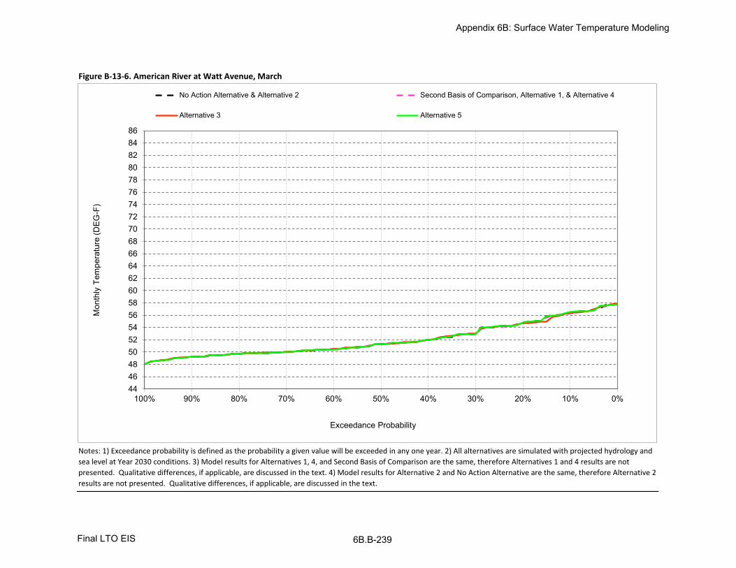
Figure B-13-6. American River at Watt Avenue, March
Notes: 1) Exceedance probability is defined as the probability a given value will be exceeded in any one year. 2) All alternatives are simulated with projected hydrology and
sea level at Year 2030 conditions. 3) Model results for Alternatives 1, 4, and Second Basis of Comparison are the same, therefore Alternatives 1 and 4 results are not
presented. Qualitative differences, if applicable, are discussed in the text. 4) Model results for Alternative 2 and No Action Alternative are the same, therefore Alternative 2
results are not presented. Qualitative differences, if applicable, are discussed in the text.
44464850525456586062646668707274767880828486
0%10%20%30%40%50%60%70%80%90%100%
Exceedance Probability
No Action Alternative & Alternative 2 Second Basis of Comparison, Alternative 1, & Alternative 4
Alternative 3 Alternative 5
Mon
thly
Tem
pera
ture
(DE
G-F
)
Appendix 6B: Surface Water Temperature Modeling
6B.B-239Final LTO EIS

Figure B-13-7. American River at Watt Avenue, April
Notes: 1) Exceedance probability is defined as the probability a given value will be exceeded in any one year. 2) All alternatives are simulated with projected hydrology and
sea level at Year 2030 conditions. 3) Model results for Alternatives 1, 4, and Second Basis of Comparison are the same, therefore Alternatives 1 and 4 results are not
presented. Qualitative differences, if applicable, are discussed in the text. 4) Model results for Alternative 2 and No Action Alternative are the same, therefore Alternative 2
results are not presented. Qualitative differences, if applicable, are discussed in the text.
44464850525456586062646668707274767880828486
0%10%20%30%40%50%60%70%80%90%100%
Exceedance Probability
No Action Alternative & Alternative 2 Second Basis of Comparison, Alternative 1, & Alternative 4
Alternative 3 Alternative 5
Mon
thly
Tem
pera
ture
(DE
G-F
)
Appendix 6B: Surface Water Temperature Modeling
6B.B-240Final LTO EIS

Figure B-13-8. American River at Watt Avenue, May
Notes: 1) Exceedance probability is defined as the probability a given value will be exceeded in any one year. 2) All alternatives are simulated with projected hydrology and
sea level at Year 2030 conditions. 3) Model results for Alternatives 1, 4, and Second Basis of Comparison are the same, therefore Alternatives 1 and 4 results are not
presented. Qualitative differences, if applicable, are discussed in the text. 4) Model results for Alternative 2 and No Action Alternative are the same, therefore Alternative 2
results are not presented. Qualitative differences, if applicable, are discussed in the text.
44464850525456586062646668707274767880828486
0%10%20%30%40%50%60%70%80%90%100%
Exceedance Probability
No Action Alternative & Alternative 2 Second Basis of Comparison, Alternative 1, & Alternative 4
Alternative 3 Alternative 5
Mon
thly
Tem
pera
ture
(DE
G-F
)
Appendix 6B: Surface Water Temperature Modeling
6B.B-241Final LTO EIS

Figure B-13-9. American River at Watt Avenue, June
Notes: 1) Exceedance probability is defined as the probability a given value will be exceeded in any one year. 2) All alternatives are simulated with projected hydrology and
sea level at Year 2030 conditions. 3) Model results for Alternatives 1, 4, and Second Basis of Comparison are the same, therefore Alternatives 1 and 4 results are not
presented. Qualitative differences, if applicable, are discussed in the text. 4) Model results for Alternative 2 and No Action Alternative are the same, therefore Alternative 2
results are not presented. Qualitative differences, if applicable, are discussed in the text.
44464850525456586062646668707274767880828486
0%10%20%30%40%50%60%70%80%90%100%
Exceedance Probability
No Action Alternative & Alternative 2 Second Basis of Comparison, Alternative 1, & Alternative 4
Alternative 3 Alternative 5
Mon
thly
Tem
pera
ture
(DE
G-F
)
Appendix 6B: Surface Water Temperature Modeling
6B.B-242Final LTO EIS

Figure B-13-10. American River at Watt Avenue, July
Notes: 1) Exceedance probability is defined as the probability a given value will be exceeded in any one year. 2) All alternatives are simulated with projected hydrology and
sea level at Year 2030 conditions. 3) Model results for Alternatives 1, 4, and Second Basis of Comparison are the same, therefore Alternatives 1 and 4 results are not
presented. Qualitative differences, if applicable, are discussed in the text. 4) Model results for Alternative 2 and No Action Alternative are the same, therefore Alternative 2
results are not presented. Qualitative differences, if applicable, are discussed in the text.
44464850525456586062646668707274767880828486
0%10%20%30%40%50%60%70%80%90%100%
Exceedance Probability
No Action Alternative & Alternative 2 Second Basis of Comparison, Alternative 1, & Alternative 4
Alternative 3 Alternative 5
Mon
thly
Tem
pera
ture
(DE
G-F
)
Appendix 6B: Surface Water Temperature Modeling
6B.B-243Final LTO EIS

Figure B-13-11. American River at Watt Avenue, August
Notes: 1) Exceedance probability is defined as the probability a given value will be exceeded in any one year. 2) All alternatives are simulated with projected hydrology and
sea level at Year 2030 conditions. 3) Model results for Alternatives 1, 4, and Second Basis of Comparison are the same, therefore Alternatives 1 and 4 results are not
presented. Qualitative differences, if applicable, are discussed in the text. 4) Model results for Alternative 2 and No Action Alternative are the same, therefore Alternative 2
results are not presented. Qualitative differences, if applicable, are discussed in the text.
44464850525456586062646668707274767880828486
0%10%20%30%40%50%60%70%80%90%100%
Exceedance Probability
No Action Alternative & Alternative 2 Second Basis of Comparison, Alternative 1, & Alternative 4
Alternative 3 Alternative 5
Mon
thly
Tem
pera
ture
(DE
G-F
)
Appendix 6B: Surface Water Temperature Modeling
Final LTO EIS 6B.B-244

Figure B-13-12. American River at Watt Avenue, September
Notes: 1) Exceedance probability is defined as the probability a given value will be exceeded in any one year. 2) All alternatives are simulated with projected hydrology and
sea level at Year 2030 conditions. 3) Model results for Alternatives 1, 4, and Second Basis of Comparison are the same, therefore Alternatives 1 and 4 results are not
presented. Qualitative differences, if applicable, are discussed in the text. 4) Model results for Alternative 2 and No Action Alternative are the same, therefore Alternative 2
results are not presented. Qualitative differences, if applicable, are discussed in the text.
44464850525456586062646668707274767880828486
0%10%20%30%40%50%60%70%80%90%100%
Exceedance Probability
No Action Alternative & Alternative 2 Second Basis of Comparison, Alternative 1, & Alternative 4
Alternative 3 Alternative 5
Mon
thly
Tem
pera
ture
(DE
G-F
)
Appendix 6B: Surface Water Temperature Modeling
Final LTO EIS 6B.B-245

Oct Nov Dec Jan Feb Mar Apr May Jun Jul Aug Sep
10% 67 58 53 48 50 56 63 68 73 73 73 7120% 66 58 52 48 50 55 60 67 70 70 72 7030% 65 58 51 47 49 53 59 65 69 69 70 6940% 64 57 51 47 48 52 58 64 67 68 69 6850% 64 57 50 47 48 51 57 62 66 68 69 6860% 64 57 49 46 47 50 56 61 65 68 68 6770% 63 56 49 46 47 50 55 60 64 67 68 6680% 63 56 48 45 46 50 54 59 63 67 67 6690% 61 56 47 45 46 49 53 57 62 67 66 65
Full Simulation Periodb 64 57 50 47 48 52 57 63 66 69 69 68
Wet (32%) 61 55 47 46 47 50 55 59 63 67 67 66Above Normal (16%) 65 57 50 47 47 50 56 62 66 67 68 67Below Normal (13%) 63 56 50 47 48 52 59 64 68 68 70 69
Dry (24%) 64 57 50 47 49 53 58 64 68 69 70 69Critical (15%) 66 58 50 47 51 56 61 67 70 74 72 71
Oct Nov Dec Jan Feb Mar Apr May Jun Jul Aug Sep
10% 67 58 53 49 50 56 62 68 71 73 73 7120% 66 58 52 48 49 55 60 66 70 69 72 7130% 65 58 51 48 49 53 59 65 68 69 70 6940% 65 57 50 47 48 52 58 64 67 68 69 6950% 64 57 50 47 48 51 57 62 66 68 69 6860% 64 57 49 46 47 50 56 61 65 67 68 6870% 63 56 49 46 47 50 55 60 64 67 67 6780% 63 56 48 45 46 50 54 59 63 67 66 6790% 61 56 47 45 46 49 53 57 62 67 65 66
Full Simulation Periodb 64 57 50 47 48 52 57 63 66 69 69 68
Wet (32%) 61 55 47 46 47 50 55 59 63 67 66 67Above Normal (16%) 64 57 50 47 47 50 56 62 66 67 68 68Below Normal (13%) 63 56 51 47 48 52 59 64 66 68 69 69
Dry (24%) 65 57 50 47 49 53 59 64 68 69 70 69Critical (15%) 66 58 50 47 51 56 61 66 71 74 72 71
Oct Nov Dec Jan Feb Mar Apr May Jun Jul Aug Sep
0.1 -0.2 0.0 0.2 0.4 0.1 -0.1 -0.2 0.3 -1.9 0.1 -0.4 0.10.2 -0.2 -0.1 0.0 0.1 0.0 -0.1 -0.2 -0.3 -0.9 -0.6 -0.2 0.30.3 0.0 0.0 0.3 0.3 0.0 0.1 -0.1 0.0 -0.3 -0.2 -0.2 0.10.4 0.1 0.0 -0.1 0.2 0.0 0.0 0.0 0.0 -0.2 -0.1 -0.2 0.40.5 0.1 -0.1 -0.1 0.0 0.0 0.0 0.0 0.0 -0.1 -0.2 -0.1 0.20.6 -0.1 0.0 0.2 0.0 0.1 0.0 0.0 0.1 -0.1 -0.2 -0.3 0.40.7 0.1 0.0 0.3 0.2 0.0 0.0 0.0 0.0 0.0 -0.3 -0.3 0.80.8 -0.1 -0.1 0.2 0.0 0.0 0.0 0.0 0.0 0.0 -0.2 -0.4 0.80.9 -0.2 0.0 -0.1 0.0 0.0 0.0 0.0 0.0 0.1 0.1 -0.2 1.4
Full Simulation Periodb
0.0 0.0 0.2 0.1 0.0 0.0 -0.1 0.0 -0.2 -0.2 -0.2 0.5
Wet (32%) -0.1 -0.1 0.2 0.1 0.0 0.0 0.0 0.0 0.0 -0.1 -0.5 1.1Above Normal (16%) -0.2 -0.3 0.1 0.2 0.0 0.0 0.0 0.0 -0.1 -0.2 0.1 0.5Below Normal (13%) 0.1 0.1 0.3 0.3 0.0 0.0 -0.3 0.1 -1.6 -0.3 -0.6 0.2
Dry (24%) 0.1 0.0 0.1 0.1 0.0 0.0 0.0 0.1 -0.2 -0.3 0.1 0.0
Critical (15%) 0.1 0.2 0.1 0.1 0.0 0.0 -0.2 -0.2 0.5 0.1 -0.1 0.1
a Exceedance probability is defined as the probability a given value will be exceeded in any one year.
b Based on an 81-year simulation period.
Probability of Exceedancea
Long Term
Water Year Typesc
c As defined by the Sacramento Valley 40-30-30 Index Water Year Hydrologic Classification (SWRCB D-1641, 1999); projected to Year 2030.
Notes: 1) All alternatives are simulated with projected hydrology and sea level at Year 2030 conditions. 2) Model results for Alternatives 1, 4, and Second Basis of Comparison are the same,
therefore Second Basis of Comparison and Alternative 4 results are not presented. Qualitative differences, if applicable, are discussed in the text. 3) Model results for Alternative 2 and No Action
Alternative are the same, therefore Alternative 2 results are not presented. Qualitative differences, if applicable, are discussed in the text.
Probability of Exceedancea
Long Term
Water Year Typesc
Alternative 1 minus No Action Alternative
Statistic
Monthly Temperature (DEG-F)
Long Term
Water Year Typesc
Alternative 1
Statistic
Monthly Temperature (DEG-F)
Table B-13-1. American River at Watt Avenue, Monthly Temperature
No Action Alternative
Statistic
Monthly Temperature (DEG-F)
Probability of Exceedancea
Appendix 6B: Surface Water Temperature Modeling
Final LTO EIS 6B.B-246

Oct Nov Dec Jan Feb Mar Apr May Jun Jul Aug Sep
10% 67 58 53 48 50 56 63 68 73 73 73 7120% 66 58 52 48 50 55 60 67 70 70 72 7030% 65 58 51 47 49 53 59 65 69 69 70 6940% 64 57 51 47 48 52 58 64 67 68 69 6850% 64 57 50 47 48 51 57 62 66 68 69 6860% 64 57 49 46 47 50 56 61 65 68 68 6770% 63 56 49 46 47 50 55 60 64 67 68 6680% 63 56 48 45 46 50 54 59 63 67 67 6690% 61 56 47 45 46 49 53 57 62 67 66 65
Full Simulation Periodb 64 57 50 47 48 52 57 63 66 69 69 68
Wet (32%) 61 55 47 46 47 50 55 59 63 67 67 66Above Normal (16%) 65 57 50 47 47 50 56 62 66 67 68 67Below Normal (13%) 63 56 50 47 48 52 59 64 68 68 70 69
Dry (24%) 64 57 50 47 49 53 58 64 68 69 70 69Critical (15%) 66 58 50 47 51 56 61 67 70 74 72 71
Oct Nov Dec Jan Feb Mar Apr May Jun Jul Aug Sep
10% 67 58 53 49 50 56 63 68 72 73 73 7120% 66 58 52 48 50 55 60 66 69 70 72 7030% 65 58 51 48 49 53 59 65 68 69 70 6940% 64 57 50 47 48 52 58 64 67 68 69 6950% 64 57 50 47 48 51 57 62 66 68 68 6860% 64 57 49 46 47 50 56 61 64 68 68 6870% 63 57 49 46 47 50 55 60 64 67 67 6780% 63 56 48 45 46 50 54 59 63 67 66 6790% 61 56 47 45 46 49 53 57 62 66 66 66
Full Simulation Periodb 64 57 50 47 48 52 57 63 66 69 69 68
Wet (32%) 61 54 48 46 47 50 55 59 63 67 66 67Above Normal (16%) 65 57 50 47 47 50 56 62 66 67 68 68Below Normal (13%) 63 57 51 47 48 52 59 64 67 68 69 69
Dry (24%) 65 57 50 47 49 53 59 64 68 69 70 69Critical (15%) 66 58 50 47 51 55 61 66 71 74 73 71
Oct Nov Dec Jan Feb Mar Apr May Jun Jul Aug Sep
0.1 -0.2 0.0 0.1 0.4 0.1 0.0 0.1 0.3 -0.4 -0.2 0.2 0.20.2 0.0 0.0 0.0 0.2 0.0 0.0 0.0 -0.2 -1.1 0.1 -0.3 0.00.3 0.1 0.0 0.4 0.2 0.0 0.0 0.1 0.2 -0.4 -0.1 0.1 0.00.4 0.0 0.0 -0.1 0.3 0.0 0.0 0.0 0.0 0.1 0.0 -0.2 0.20.5 0.0 0.0 0.2 0.0 0.0 0.0 0.0 0.0 -0.1 0.1 -0.1 0.20.6 -0.2 -0.1 0.2 0.1 0.1 0.0 0.0 0.0 -0.3 0.0 -0.1 0.40.7 0.1 0.1 0.3 0.2 0.0 0.0 0.0 0.0 -0.1 -0.2 -0.2 0.90.8 -0.1 0.0 0.2 0.1 0.0 0.0 0.0 0.0 0.0 -0.1 -0.6 0.80.9 -0.2 0.0 0.0 0.0 0.0 0.0 0.0 0.0 0.1 -0.2 -0.1 0.8
Full Simulation Periodb 0.0 0.0 0.2 0.1 0.0 0.0 0.0 0.1 -0.1 0.0 -0.2 0.4
Wet (32%) 0.0 -0.1 0.2 0.1 0.0 0.0 0.0 0.0 -0.1 0.1 -0.4 1.0Above Normal (16%) -0.1 -0.2 0.0 0.1 0.0 0.0 0.0 0.0 -0.2 -0.2 0.3 0.6Below Normal (13%) 0.1 0.3 0.4 0.3 0.1 0.0 -0.1 0.1 -0.5 -0.1 -0.6 0.1
Dry (24%) 0.1 0.0 0.1 0.1 0.0 0.0 0.1 0.2 -0.1 0.0 -0.1 -0.1
Critical (15%) 0.0 0.1 0.1 0.1 0.0 -0.1 0.0 -0.2 0.3 0.0 0.1 0.2
a Exceedance probability is defined as the probability a given value will be exceeded in any one year.
b Based on an 81-year simulation period.
Probability of Exceedancea
Long Term
Water Year Typesc
c As defined by the Sacramento Valley 40-30-30 Index Water Year Hydrologic Classification (SWRCB D-1641, 1999); projected to Year 2030.
Notes: 1) All alternatives are simulated with projected hydrology and sea level at Year 2030 conditions. 2) Model results for Alternatives 1, 4, and Second Basis of Comparison are the same,
therefore Alternative 1 and 4 results are not presented. Qualitative differences, if applicable, are discussed in the text. 3) Model results for Alternative 2 and No Action Alternative are the same,
therefore Alternative 2 results are not presented. Qualitative differences, if applicable, are discussed in the text.
Probability of Exceedancea
Long Term
Water Year Typesc
Alternative 3 minus No Action Alternative
Statistic
Monthly Temperature (DEG-F)
Long Term
Water Year Typesc
Alternative 3
Statistic
Monthly Temperature (DEG-F)
Table B-13-2. American River at Watt Avenue, Monthly Temperature
No Action Alternative
Statistic
Monthly Temperature (DEG-F)
Probability of Exceedancea
Appendix 6B: Surface Water Temperature Modeling
Final LTO EIS 6B.B-247

Oct Nov Dec Jan Feb Mar Apr May Jun Jul Aug Sep
10% 67 58 53 48 50 56 63 68 73 73 73 7120% 66 58 52 48 50 55 60 67 70 70 72 7030% 65 58 51 47 49 53 59 65 69 69 70 6940% 64 57 51 47 48 52 58 64 67 68 69 6850% 64 57 50 47 48 51 57 62 66 68 69 6860% 64 57 49 46 47 50 56 61 65 68 68 6770% 63 56 49 46 47 50 55 60 64 67 68 6680% 63 56 48 45 46 50 54 59 63 67 67 6690% 61 56 47 45 46 49 53 57 62 67 66 65
Full Simulation Periodb 64 57 50 47 48 52 57 63 66 69 69 68
Wet (32%) 61 55 47 46 47 50 55 59 63 67 67 66Above Normal (16%) 65 57 50 47 47 50 56 62 66 67 68 67Below Normal (13%) 63 56 50 47 48 52 59 64 68 68 70 69
Dry (24%) 64 57 50 47 49 53 58 64 68 69 70 69Critical (15%) 66 58 50 47 51 56 61 67 70 74 72 71
Oct Nov Dec Jan Feb Mar Apr May Jun Jul Aug Sep
10% 67 58 53 48 50 56 63 68 73 73 73 7120% 66 58 52 48 50 55 60 67 70 70 72 7030% 65 58 51 47 49 53 59 65 68 69 70 6940% 64 57 51 47 48 52 58 64 67 68 69 6850% 64 57 50 47 48 51 57 62 66 68 69 6860% 64 57 49 46 47 50 56 61 65 67 68 6770% 63 56 48 46 47 50 55 60 64 67 68 6680% 63 56 48 45 46 50 54 59 63 67 67 6690% 61 56 47 45 46 49 53 57 62 66 66 65
Full Simulation Periodb 64 57 50 47 48 52 57 63 66 69 69 68
Wet (32%) 61 55 47 46 47 50 55 59 63 67 67 66Above Normal (16%) 65 57 50 47 47 50 56 62 66 67 68 67Below Normal (13%) 63 56 50 47 48 52 59 64 68 68 70 69
Dry (24%) 64 57 50 47 49 53 58 64 68 69 70 69Critical (15%) 66 58 50 47 51 56 61 67 70 74 72 72
Oct Nov Dec Jan Feb Mar Apr May Jun Jul Aug Sep
0.1 0.0 0.0 0.0 0.0 0.0 0.1 0.1 0.5 0.2 -0.1 0.1 0.20.2 0.0 -0.1 0.1 0.0 0.0 0.0 0.0 0.3 -0.3 -0.3 -0.2 0.20.3 0.1 0.0 0.1 0.0 0.0 0.0 0.0 0.0 -0.3 -0.1 -0.1 -0.1
0.4 -0.1 0.0 0.0 0.0 0.0 0.0 0.0 0.0 0.1 -0.1 -0.1 -0.2
0.5 -0.1 0.0 0.0 0.0 0.0 0.0 0.0 0.1 0.0 -0.1 0.0 0.0
0.6 -0.2 0.0 0.0 0.0 0.0 0.0 0.0 0.0 0.0 -0.1 -0.1 0.00.7 0.0 0.0 0.0 0.0 0.0 0.0 0.0 0.0 0.0 -0.1 -0.1 0.0
0.8 0.0 -0.1 0.0 0.0 0.0 0.0 0.0 0.0 0.0 0.0 0.4 0.00.9 0.1 -0.1 -0.1 -0.1 0.0 0.0 0.0 0.0 0.1 -0.1 0.2 0.1
Full Simulation Periodb
0.0 0.0 0.0 0.0 0.0 0.0 0.0 0.1 0.0 -0.2 0.0 0.1
Wet (32%) 0.0 0.0 0.0 0.0 0.0 0.0 0.0 0.0 0.0 -0.1 0.1 0.0Above Normal (16%) 0.0 -0.2 0.0 0.0 0.0 0.0 0.0 0.0 0.0 0.0 0.0 0.0Below Normal (13%) 0.0 0.0 -0.1 -0.1 0.0 0.0 0.0 0.1 0.1 -0.1 0.1 0.1
Dry (24%) 0.0 0.0 0.0 0.0 0.0 0.0 0.0 0.2 0.1 -0.2 0.0 0.0
Critical (15%) 0.0 -0.1 0.0 0.0 0.0 0.1 0.1 0.0 -0.3 -0.5 -0.1 0.5
a Exceedance probability is defined as the probability a given value will be exceeded in any one year.
b Based on an 81-year simulation period.
Probability of Exceedancea
Long Term
Water Year Typesc
c As defined by the Sacramento Valley 40-30-30 Index Water Year Hydrologic Classification (SWRCB D-1641, 1999); projected to Year 2030.
Notes: 1) All alternatives are simulated with projected hydrology and sea level at Year 2030 conditions. 2) Model results for Alternatives 1, 4, and Second Basis of Comparison are the same,
therefore Alternative 1 and 4 results are not presented. Qualitative differences, if applicable, are discussed in the text. 3) Model results for Alternative 2 and No Action Alternative are the same,
therefore Alternative 2 results are not presented. Qualitative differences, if applicable, are discussed in the text.
Probability of Exceedancea
Long Term
Water Year Typesc
Alternative 5 minus No Action Alternative
Statistic
Monthly Temperature (DEG-F)
Long Term
Water Year Typesc
Alternative 5
Statistic
Monthly Temperature (DEG-F)
Table B-13-3. American River at Watt Avenue, Monthly Temperature
No Action Alternative
Statistic
Monthly Temperature (DEG-F)
Probability of Exceedancea
Appendix 6B: Surface Water Temperature Modeling
Final LTO EIS 6B.B-248

Oct Nov Dec Jan Feb Mar Apr May Jun Jul Aug Sep
10% 67 58 53 49 50 56 62 68 71 73 73 7120% 66 58 52 48 49 55 60 66 70 69 72 7130% 65 58 51 48 49 53 59 65 68 69 70 6940% 65 57 50 47 48 52 58 64 67 68 69 6950% 64 57 50 47 48 51 57 62 66 68 69 6860% 64 57 49 46 47 50 56 61 65 67 68 6870% 63 56 49 46 47 50 55 60 64 67 67 6780% 63 56 48 45 46 50 54 59 63 67 66 6790% 61 56 47 45 46 49 53 57 62 67 65 66
Full Simulation Periodb 64 57 50 47 48 52 57 63 66 69 69 68
Wet (32%) 61 55 47 46 47 50 55 59 63 67 66 67Above Normal (16%) 64 57 50 47 47 50 56 62 66 67 68 68Below Normal (13%) 63 56 51 47 48 52 59 64 66 68 69 69
Dry (24%) 65 57 50 47 49 53 59 64 68 69 70 69Critical (15%) 66 58 50 47 51 56 61 66 71 74 72 71
Oct Nov Dec Jan Feb Mar Apr May Jun Jul Aug Sep
10% 67 58 53 48 50 56 63 68 73 73 73 7120% 66 58 52 48 50 55 60 67 70 70 72 7030% 65 58 51 47 49 53 59 65 69 69 70 6940% 64 57 51 47 48 52 58 64 67 68 69 6850% 64 57 50 47 48 51 57 62 66 68 69 6860% 64 57 49 46 47 50 56 61 65 68 68 6770% 63 56 49 46 47 50 55 60 64 67 68 6680% 63 56 48 45 46 50 54 59 63 67 67 6690% 61 56 47 45 46 49 53 57 62 67 66 65
Full Simulation Periodb 64 57 50 47 48 52 57 63 66 69 69 68
Wet (32%) 61 55 47 46 47 50 55 59 63 67 67 66Above Normal (16%) 65 57 50 47 47 50 56 62 66 67 68 67Below Normal (13%) 63 56 50 47 48 52 59 64 68 68 70 69
Dry (24%) 64 57 50 47 49 53 58 64 68 69 70 69Critical (15%) 66 58 50 47 51 56 61 67 70 74 72 71
Oct Nov Dec Jan Feb Mar Apr May Jun Jul Aug Sep
0.1 0.2 0.0 -0.2 -0.4 -0.1 0.1 0.2 -0.3 1.9 -0.1 0.4 -0.1
0.2 0.2 0.1 0.0 -0.1 0.0 0.1 0.2 0.3 0.9 0.6 0.2 -0.3
0.3 0.0 0.0 -0.3 -0.3 0.0 -0.1 0.1 0.0 0.3 0.2 0.2 -0.1
0.4 -0.1 0.0 0.1 -0.2 0.0 0.0 0.0 0.0 0.2 0.1 0.2 -0.4
0.5 -0.1 0.1 0.1 0.0 0.0 0.0 0.0 0.0 0.1 0.2 0.1 -0.2
0.6 0.1 0.0 -0.2 0.0 -0.1 0.0 0.0 -0.1 0.1 0.2 0.3 -0.4
0.7 -0.1 0.0 -0.3 -0.2 0.0 0.0 0.0 0.0 0.0 0.3 0.3 -0.8
0.8 0.1 0.1 -0.2 0.0 0.0 0.0 0.0 0.0 0.0 0.2 0.4 -0.8
0.9 0.2 0.0 0.1 0.0 0.0 0.0 0.0 0.0 -0.1 -0.1 0.2 -1.4
Full Simulation Periodb 0.0 0.0 -0.2 -0.1 0.0 0.0 0.1 0.0 0.2 0.2 0.2 -0.5
Wet (32%) 0.1 0.1 -0.2 -0.1 0.0 0.0 0.0 0.0 0.0 0.1 0.5 -1.1
Above Normal (16%) 0.2 0.3 -0.1 -0.2 0.0 0.0 0.0 0.0 0.1 0.2 -0.1 -0.5
Below Normal (13%) -0.1 -0.1 -0.3 -0.3 0.0 0.0 0.3 -0.1 1.6 0.3 0.6 -0.2
Dry (24%) -0.1 0.0 -0.1 -0.1 0.0 0.0 0.0 -0.1 0.2 0.3 -0.1 0.0Critical (15%) -0.1 -0.2 -0.1 -0.1 0.0 0.0 0.2 0.2 -0.5 -0.1 0.1 -0.1
a Exceedance probability is defined as the probability a given value will be exceeded in any one year.
b Based on an 81-year simulation period.
Probability of Exceedancea
Long Term
Water Year Typesc
c As defined by the Sacramento Valley 40-30-30 Index Water Year Hydrologic Classification (SWRCB D-1641, 1999); projected to Year 2030.
Notes: 1) All alternatives are simulated with projected hydrology and sea level at Year 2030 conditions. 2) Model results for Alternatives 1, 4, and Second Basis of Comparison are the same,
therefore Alternative 1 and 4 results are not presented. Qualitative differences, if applicable, are discussed in the text. 3) Model results for Alternative 2 and No Action Alternative are the same,
therefore Alternative 2 results are not presented. Qualitative differences, if applicable, are discussed in the text.
Probability of Exceedancea
Long Term
Water Year Typesc
No Action Alternative minus Second Basis of Comparison
Statistic
Monthly Temperature (DEG-F)
Long Term
Water Year Typesc
No Action Alternative
Statistic
Monthly Temperature (DEG-F)
Table B-13-4. American River at Watt Avenue, Monthly Temperature
Second Basis of Comparison
Statistic
Monthly Temperature (DEG-F)
Probability of Exceedancea
Appendix 6B: Surface Water Temperature Modeling
Final LTO EIS 6B.B-249

Oct Nov Dec Jan Feb Mar Apr May Jun Jul Aug Sep
10% 67 58 53 49 50 56 62 68 71 73 73 7120% 66 58 52 48 49 55 60 66 70 69 72 7130% 65 58 51 48 49 53 59 65 68 69 70 6940% 65 57 50 47 48 52 58 64 67 68 69 6950% 64 57 50 47 48 51 57 62 66 68 69 6860% 64 57 49 46 47 50 56 61 65 67 68 6870% 63 56 49 46 47 50 55 60 64 67 67 6780% 63 56 48 45 46 50 54 59 63 67 66 6790% 61 56 47 45 46 49 53 57 62 67 65 66
Full Simulation Periodb 64 57 50 47 48 52 57 63 66 69 69 68
Wet (32%) 61 55 47 46 47 50 55 59 63 67 66 67Above Normal (16%) 64 57 50 47 47 50 56 62 66 67 68 68Below Normal (13%) 63 56 51 47 48 52 59 64 66 68 69 69
Dry (24%) 65 57 50 47 49 53 59 64 68 69 70 69Critical (15%) 66 58 50 47 51 56 61 66 71 74 72 71
Oct Nov Dec Jan Feb Mar Apr May Jun Jul Aug Sep
10% 67 58 53 49 50 56 63 68 72 73 73 7120% 66 58 52 48 50 55 60 66 69 70 72 7030% 65 58 51 48 49 53 59 65 68 69 70 6940% 64 57 50 47 48 52 58 64 67 68 69 6950% 64 57 50 47 48 51 57 62 66 68 68 6860% 64 57 49 46 47 50 56 61 64 68 68 6870% 63 57 49 46 47 50 55 60 64 67 67 6780% 63 56 48 45 46 50 54 59 63 67 66 6790% 61 56 47 45 46 49 53 57 62 66 66 66
Full Simulation Periodb 64 57 50 47 48 52 57 63 66 69 69 68
Wet (32%) 61 54 48 46 47 50 55 59 63 67 66 67Above Normal (16%) 65 57 50 47 47 50 56 62 66 67 68 68Below Normal (13%) 63 57 51 47 48 52 59 64 67 68 69 69
Dry (24%) 65 57 50 47 49 53 59 64 68 69 70 69Critical (15%) 66 58 50 47 51 55 61 66 71 74 73 71
Oct Nov Dec Jan Feb Mar Apr May Jun Jul Aug Sep
0.1 0.0 0.0 -0.1 0.0 0.0 0.1 0.4 0.0 1.5 -0.2 0.6 0.00.2 0.2 0.0 0.0 0.1 0.0 0.0 0.2 0.1 -0.3 0.7 -0.1 -0.3
0.3 0.1 0.0 0.1 0.0 0.0 0.0 0.2 0.2 -0.1 0.0 0.3 -0.1
0.4 -0.1 0.0 0.0 0.0 0.0 0.0 0.0 0.0 0.3 0.1 0.0 -0.2
0.5 -0.1 0.0 0.3 0.0 0.0 0.0 0.0 0.0 0.0 0.3 0.0 0.0
0.6 0.0 -0.1 0.0 0.1 0.0 0.0 0.0 0.0 -0.2 0.2 0.2 0.0
0.7 0.0 0.1 0.0 0.0 0.0 0.0 0.0 0.0 -0.1 0.0 0.1 0.10.8 0.0 0.1 0.0 0.0 0.0 0.0 0.0 0.0 0.0 0.1 -0.2 0.0
0.9 0.0 0.0 0.1 0.0 0.0 0.0 0.0 0.0 0.0 -0.2 0.1 -0.5
Full Simulation Periodb 0.0 0.0 0.0 0.0 0.0 0.0 0.0 0.0 0.1 0.1 0.1 0.0
Wet (32%) 0.0 0.0 0.0 0.0 0.0 0.0 0.0 0.0 -0.1 0.1 0.1 -0.1
Above Normal (16%) 0.2 0.2 -0.1 -0.1 0.0 0.0 0.0 0.0 -0.1 0.0 0.2 0.1Below Normal (13%) 0.0 0.2 0.0 0.0 0.0 0.0 0.2 0.1 1.0 0.1 0.0 -0.1
Dry (24%) -0.1 0.0 0.1 0.0 0.0 0.0 0.0 0.1 0.0 0.3 -0.2 -0.1
Critical (15%) -0.1 -0.1 -0.1 0.0 0.0 -0.1 0.1 0.0 -0.2 -0.1 0.2 0.1
a Exceedance probability is defined as the probability a given value will be exceeded in any one year.
b Based on an 81-year simulation period.
Probability of Exceedancea
Long Term
Water Year Typesc
c As defined by the Sacramento Valley 40-30-30 Index Water Year Hydrologic Classification (SWRCB D-1641, 1999); projected to Year 2030.
Notes: 1) All alternatives are simulated with projected hydrology and sea level at Year 2030 conditions. 2) Model results for Alternatives 1, 4, and Second Basis of Comparison are the same,
therefore Alternative 1 and 4 results are not presented. Qualitative differences, if applicable, are discussed in the text. 3) Model results for Alternative 2 and No Action Alternative are the same,
therefore Alternative 2 results are not presented. Qualitative differences, if applicable, are discussed in the text.
Probability of Exceedancea
Long Term
Water Year Typesc
Alternative 3 minus Second Basis of Comparison
Statistic
Monthly Temperature (DEG-F)
Long Term
Water Year Typesc
Alternative 3
Statistic
Monthly Temperature (DEG-F)
Table B-13-5. American River at Watt Avenue, Monthly Temperature
Second Basis of Comparison
Statistic
Monthly Temperature (DEG-F)
Probability of Exceedancea
Appendix 6B: Surface Water Temperature Modeling
Final LTO EIS 6B.B-250

Oct Nov Dec Jan Feb Mar Apr May Jun Jul Aug Sep
10% 67 58 53 49 50 56 62 68 71 73 73 7120% 66 58 52 48 49 55 60 66 70 69 72 7130% 65 58 51 48 49 53 59 65 68 69 70 6940% 65 57 50 47 48 52 58 64 67 68 69 6950% 64 57 50 47 48 51 57 62 66 68 69 6860% 64 57 49 46 47 50 56 61 65 67 68 6870% 63 56 49 46 47 50 55 60 64 67 67 6780% 63 56 48 45 46 50 54 59 63 67 66 6790% 61 56 47 45 46 49 53 57 62 67 65 66
Full Simulation Periodb 64 57 50 47 48 52 57 63 66 69 69 68
Wet (32%) 61 55 47 46 47 50 55 59 63 67 66 67Above Normal (16%) 64 57 50 47 47 50 56 62 66 67 68 68Below Normal (13%) 63 56 51 47 48 52 59 64 66 68 69 69
Dry (24%) 65 57 50 47 49 53 59 64 68 69 70 69Critical (15%) 66 58 50 47 51 56 61 66 71 74 72 71
Oct Nov Dec Jan Feb Mar Apr May Jun Jul Aug Sep
10% 67 58 53 48 50 56 63 68 73 73 73 7120% 66 58 52 48 50 55 60 67 70 70 72 7030% 65 58 51 47 49 53 59 65 68 69 70 6940% 64 57 51 47 48 52 58 64 67 68 69 6850% 64 57 50 47 48 51 57 62 66 68 69 6860% 64 57 49 46 47 50 56 61 65 67 68 6770% 63 56 48 46 47 50 55 60 64 67 68 6680% 63 56 48 45 46 50 54 59 63 67 67 6690% 61 56 47 45 46 49 53 57 62 66 66 65
Full Simulation Periodb 64 57 50 47 48 52 57 63 66 69 69 68
Wet (32%) 61 55 47 46 47 50 55 59 63 67 67 66Above Normal (16%) 65 57 50 47 47 50 56 62 66 67 68 67Below Normal (13%) 63 56 50 47 48 52 59 64 68 68 70 69
Dry (24%) 64 57 50 47 49 53 58 64 68 69 70 69Critical (15%) 66 58 50 47 51 56 61 67 70 74 72 72
Oct Nov Dec Jan Feb Mar Apr May Jun Jul Aug Sep
0.1 0.2 0.0 -0.2 -0.4 -0.1 0.2 0.3 0.2 2.1 -0.2 0.5 0.00.2 0.3 0.0 0.1 -0.1 0.0 0.1 0.3 0.6 0.6 0.3 0.0 -0.1
0.3 0.1 -0.1 -0.3 -0.3 0.0 -0.1 0.1 0.0 0.0 0.0 0.1 -0.2
0.4 -0.2 0.0 0.1 -0.2 -0.1 0.0 0.0 0.0 0.3 0.0 0.2 -0.6
0.5 -0.2 0.0 0.0 0.0 0.0 0.0 0.0 0.1 0.1 0.1 0.0 -0.2
0.6 -0.1 0.0 -0.1 0.0 -0.1 -0.1 0.0 0.0 0.1 0.2 0.1 -0.4
0.7 -0.1 0.0 -0.3 -0.2 0.0 0.0 0.0 0.0 0.0 0.2 0.2 -0.8
0.8 0.1 0.1 -0.1 0.0 0.0 0.0 0.0 0.0 0.0 0.2 0.8 -0.8
0.9 0.4 -0.1 0.0 -0.1 0.0 0.0 0.0 0.0 0.0 -0.2 0.4 -1.3
Full Simulation Periodb
0.0 0.0 -0.2 -0.1 0.0 0.0 0.1 0.0 0.2 0.0 0.3 -0.4
Wet (32%) 0.0 0.0 -0.2 -0.1 0.0 0.0 0.0 0.0 0.0 -0.1 0.6 -1.1
Above Normal (16%) 0.2 0.1 -0.1 -0.2 0.0 0.0 0.0 0.0 0.2 0.2 -0.1 -0.5
Below Normal (13%) -0.1 -0.1 -0.4 -0.3 -0.1 0.0 0.3 0.0 1.6 0.2 0.7 -0.1
Dry (24%) -0.1 0.0 0.0 -0.1 0.0 0.0 0.0 0.1 0.3 0.1 -0.1 0.0Critical (15%) -0.1 -0.2 -0.2 -0.1 0.0 0.1 0.3 0.2 -0.7 -0.6 0.1 0.3
a Exceedance probability is defined as the probability a given value will be exceeded in any one year.
b Based on an 81-year simulation period.
Probability of Exceedancea
Long Term
Water Year Typesc
c As defined by the Sacramento Valley 40-30-30 Index Water Year Hydrologic Classification (SWRCB D-1641, 1999); projected to Year 2030.
Notes: 1) All alternatives are simulated with projected hydrology and sea level at Year 2030 conditions. 2) Model results for Alternatives 1, 4, and Second Basis of Comparison are the same,
therefore Alternative 1 and 4 results are not presented. Qualitative differences, if applicable, are discussed in the text. 3) Model results for Alternative 2 and No Action Alternative are the same,
therefore Alternative 2 results are not presented. Qualitative differences, if applicable, are discussed in the text.
Probability of Exceedancea
Long Term
Water Year Typesc
Alternative 5 minus Second Basis of Comparison
Statistic
Monthly Temperature (DEG-F)
Long Term
Water Year Typesc
Alternative 5
Statistic
Monthly Temperature (DEG-F)
Table B-13-6. American River at Watt Avenue, Monthly Temperature
Second Basis of Comparison
Statistic
Monthly Temperature (DEG-F)
Probability of Exceedancea
Appendix 6B: Surface Water Temperature Modeling
Final LTO EIS 6B.B-251

B.14. American River at Mouth Temperature
Appendix 6B: Surface Water Temperature Modeling
Final LTO EIS 6B.B-252

Figure B-14-1. American River at the Mouth, October
Notes: 1) Exceedance probability is defined as the probability a given value will be exceeded in any one year. 2) All alternatives are simulated with projected hydrology and
sea level at Year 2030 conditions. 3) Model results for Alternatives 1, 4, and Second Basis of Comparison are the same, therefore Alternatives 1 and 4 results are not
presented. Qualitative differences, if applicable, are discussed in the text. 4) Model results for Alternative 2 and No Action Alternative are the same, therefore Alternative 2
results are not presented. Qualitative differences, if applicable, are discussed in the text.
44464850525456586062646668707274767880828486
0%10%20%30%40%50%60%70%80%90%100%
Exceedance Probability
No Action Alternative & Alternative 2 Second Basis of Comparison, Alternative 1, & Alternative 4
Alternative 3 Alternative 5
Mon
thly
Tem
pera
ture
(DE
G-F
)
Appendix 6B: Surface Water Temperature Modeling
Final LTO EIS 6B.B-253

Figure B-14-2. American River at the Mouth, November
Notes: 1) Exceedance probability is defined as the probability a given value will be exceeded in any one year. 2) All alternatives are simulated with projected hydrology and
sea level at Year 2030 conditions. 3) Model results for Alternatives 1, 4, and Second Basis of Comparison are the same, therefore Alternatives 1 and 4 results are not
presented. Qualitative differences, if applicable, are discussed in the text. 4) Model results for Alternative 2 and No Action Alternative are the same, therefore Alternative 2
results are not presented. Qualitative differences, if applicable, are discussed in the text.
44464850525456586062646668707274767880828486
0%10%20%30%40%50%60%70%80%90%100%
Exceedance Probability
No Action Alternative & Alternative 2 Second Basis of Comparison, Alternative 1, & Alternative 4
Alternative 3 Alternative 5
Mon
thly
Tem
pera
ture
(DE
G-F
)
Appendix 6B: Surface Water Temperature Modeling
Final LTO EIS 6B.B-254

Figure B-14-3. American River at the Mouth, December
Notes: 1) Exceedance probability is defined as the probability a given value will be exceeded in any one year. 2) All alternatives are simulated with projected hydrology and
sea level at Year 2030 conditions. 3) Model results for Alternatives 1, 4, and Second Basis of Comparison are the same, therefore Alternatives 1 and 4 results are not
presented. Qualitative differences, if applicable, are discussed in the text. 4) Model results for Alternative 2 and No Action Alternative are the same, therefore Alternative 2
results are not presented. Qualitative differences, if applicable, are discussed in the text.
44464850525456586062646668707274767880828486
0%10%20%30%40%50%60%70%80%90%100%
Exceedance Probability
No Action Alternative & Alternative 2 Second Basis of Comparison, Alternative 1, & Alternative 4
Alternative 3 Alternative 5
Mon
thly
Tem
pera
ture
(DE
G-F
)
Appendix 6B: Surface Water Temperature Modeling
Final LTO EIS 6B.B-255

Figure B-14-4. American River at the Mouth, January
Notes: 1) Exceedance probability is defined as the probability a given value will be exceeded in any one year. 2) All alternatives are simulated with projected hydrology and
sea level at Year 2030 conditions. 3) Model results for Alternatives 1, 4, and Second Basis of Comparison are the same, therefore Alternatives 1 and 4 results are not
presented. Qualitative differences, if applicable, are discussed in the text. 4) Model results for Alternative 2 and No Action Alternative are the same, therefore Alternative 2
results are not presented. Qualitative differences, if applicable, are discussed in the text.
44464850525456586062646668707274767880828486
0%10%20%30%40%50%60%70%80%90%100%
Exceedance Probability
No Action Alternative & Alternative 2 Second Basis of Comparison, Alternative 1, & Alternative 4
Alternative 3 Alternative 5
Mon
thly
Tem
pera
ture
(DE
G-F
)
Appendix 6B: Surface Water Temperature Modeling
Final LTO EIS 6B.B-256
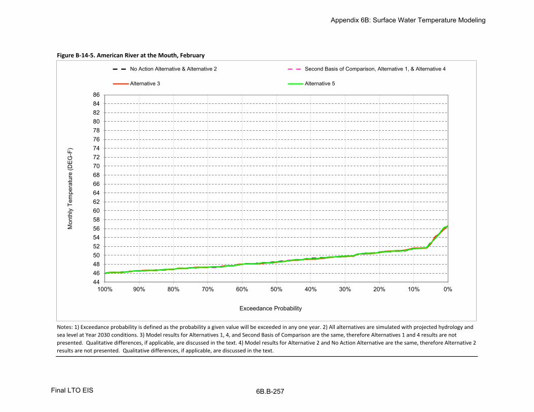
Figure B-14-5. American River at the Mouth, February
Notes: 1) Exceedance probability is defined as the probability a given value will be exceeded in any one year. 2) All alternatives are simulated with projected hydrology and
sea level at Year 2030 conditions. 3) Model results for Alternatives 1, 4, and Second Basis of Comparison are the same, therefore Alternatives 1 and 4 results are not
presented. Qualitative differences, if applicable, are discussed in the text. 4) Model results for Alternative 2 and No Action Alternative are the same, therefore Alternative 2
results are not presented. Qualitative differences, if applicable, are discussed in the text.
44464850525456586062646668707274767880828486
0%10%20%30%40%50%60%70%80%90%100%
Exceedance Probability
No Action Alternative & Alternative 2 Second Basis of Comparison, Alternative 1, & Alternative 4
Alternative 3 Alternative 5
Mon
thly
Tem
pera
ture
(DE
G-F
)
Appendix 6B: Surface Water Temperature Modeling
Final LTO EIS 6B.B-257

Figure B-14-6. American River at the Mouth, March
Notes: 1) Exceedance probability is defined as the probability a given value will be exceeded in any one year. 2) All alternatives are simulated with projected hydrology and
sea level at Year 2030 conditions. 3) Model results for Alternatives 1, 4, and Second Basis of Comparison are the same, therefore Alternatives 1 and 4 results are not
presented. Qualitative differences, if applicable, are discussed in the text. 4) Model results for Alternative 2 and No Action Alternative are the same, therefore Alternative 2
results are not presented. Qualitative differences, if applicable, are discussed in the text.
44464850525456586062646668707274767880828486
0%10%20%30%40%50%60%70%80%90%100%
Exceedance Probability
No Action Alternative & Alternative 2 Second Basis of Comparison, Alternative 1, & Alternative 4
Alternative 3 Alternative 5
Mon
thly
Tem
pera
ture
(DE
G-F
)
Appendix 6B: Surface Water Temperature Modeling
Final LTO EIS 6B.B-258

Figure B-14-7. American River at the Mouth, April
Notes: 1) Exceedance probability is defined as the probability a given value will be exceeded in any one year. 2) All alternatives are simulated with projected hydrology and
sea level at Year 2030 conditions. 3) Model results for Alternatives 1, 4, and Second Basis of Comparison are the same, therefore Alternatives 1 and 4 results are not
presented. Qualitative differences, if applicable, are discussed in the text. 4) Model results for Alternative 2 and No Action Alternative are the same, therefore Alternative 2
results are not presented. Qualitative differences, if applicable, are discussed in the text.
44464850525456586062646668707274767880828486
0%10%20%30%40%50%60%70%80%90%100%
Exceedance Probability
No Action Alternative & Alternative 2 Second Basis of Comparison, Alternative 1, & Alternative 4
Alternative 3 Alternative 5
Mon
thly
Tem
pera
ture
(DE
G-F
)
Appendix 6B: Surface Water Temperature Modeling
Final LTO EIS 6B.B-259

Figure B-14-8. American River at the Mouth, May
Notes: 1) Exceedance probability is defined as the probability a given value will be exceeded in any one year. 2) All alternatives are simulated with projected hydrology and
sea level at Year 2030 conditions. 3) Model results for Alternatives 1, 4, and Second Basis of Comparison are the same, therefore Alternatives 1 and 4 results are not
presented. Qualitative differences, if applicable, are discussed in the text. 4) Model results for Alternative 2 and No Action Alternative are the same, therefore Alternative 2
results are not presented. Qualitative differences, if applicable, are discussed in the text.
44464850525456586062646668707274767880828486
0%10%20%30%40%50%60%70%80%90%100%
Exceedance Probability
No Action Alternative & Alternative 2 Second Basis of Comparison, Alternative 1, & Alternative 4
Alternative 3 Alternative 5
Mon
thly
Tem
pera
ture
(DE
G-F
)
Appendix 6B: Surface Water Temperature Modeling
Final LTO EIS 6B.B-260

Figure B-14-9. American River at the Mouth, June
Notes: 1) Exceedance probability is defined as the probability a given value will be exceeded in any one year. 2) All alternatives are simulated with projected hydrology and
sea level at Year 2030 conditions. 3) Model results for Alternatives 1, 4, and Second Basis of Comparison are the same, therefore Alternatives 1 and 4 results are not
presented. Qualitative differences, if applicable, are discussed in the text. 4) Model results for Alternative 2 and No Action Alternative are the same, therefore Alternative 2
results are not presented. Qualitative differences, if applicable, are discussed in the text.
44464850525456586062646668707274767880828486
0%10%20%30%40%50%60%70%80%90%100%
Exceedance Probability
No Action Alternative & Alternative 2 Second Basis of Comparison, Alternative 1, & Alternative 4
Alternative 3 Alternative 5
Mon
thly
Tem
pera
ture
(DE
G-F
)
Appendix 6B: Surface Water Temperature Modeling
Final LTO EIS 6B.B-261

Figure B-14-10. American River at the Mouth, July
Notes: 1) Exceedance probability is defined as the probability a given value will be exceeded in any one year. 2) All alternatives are simulated with projected hydrology and
sea level at Year 2030 conditions. 3) Model results for Alternatives 1, 4, and Second Basis of Comparison are the same, therefore Alternatives 1 and 4 results are not
presented. Qualitative differences, if applicable, are discussed in the text. 4) Model results for Alternative 2 and No Action Alternative are the same, therefore Alternative 2
results are not presented. Qualitative differences, if applicable, are discussed in the text.
44464850525456586062646668707274767880828486
0%10%20%30%40%50%60%70%80%90%100%
Exceedance Probability
No Action Alternative & Alternative 2 Second Basis of Comparison, Alternative 1, & Alternative 4
Alternative 3 Alternative 5
Mon
thly
Tem
pera
ture
(DE
G-F
)
Appendix 6B: Surface Water Temperature Modeling
Final LTO EIS 6B.B-262

Figure B-14-11. American River at the Mouth, August
Notes: 1) Exceedance probability is defined as the probability a given value will be exceeded in any one year. 2) All alternatives are simulated with projected hydrology and
sea level at Year 2030 conditions. 3) Model results for Alternatives 1, 4, and Second Basis of Comparison are the same, therefore Alternatives 1 and 4 results are not
presented. Qualitative differences, if applicable, are discussed in the text. 4) Model results for Alternative 2 and No Action Alternative are the same, therefore Alternative 2
results are not presented. Qualitative differences, if applicable, are discussed in the text.
44464850525456586062646668707274767880828486
0%10%20%30%40%50%60%70%80%90%100%
Exceedance Probability
No Action Alternative & Alternative 2 Second Basis of Comparison, Alternative 1, & Alternative 4
Alternative 3 Alternative 5
Mon
thly
Tem
pera
ture
(DE
G-F
)
Appendix 6B: Surface Water Temperature Modeling
Final LTO EIS 6B.B-263

Figure B-14-12. American River at the Mouth, September
Notes: 1) Exceedance probability is defined as the probability a given value will be exceeded in any one year. 2) All alternatives are simulated with projected hydrology and
sea level at Year 2030 conditions. 3) Model results for Alternatives 1, 4, and Second Basis of Comparison are the same, therefore Alternatives 1 and 4 results are not
presented. Qualitative differences, if applicable, are discussed in the text. 4) Model results for Alternative 2 and No Action Alternative are the same, therefore Alternative 2
results are not presented. Qualitative differences, if applicable, are discussed in the text.
44464850525456586062646668707274767880828486
0%10%20%30%40%50%60%70%80%90%100%
Exceedance Probability
No Action Alternative & Alternative 2 Second Basis of Comparison, Alternative 1, & Alternative 4
Alternative 3 Alternative 5
Mon
thly
Tem
pera
ture
(DE
G-F
)
Appendix 6B: Surface Water Temperature Modeling
Final LTO EIS 6B.B-264

Oct Nov Dec Jan Feb Mar Apr May Jun Jul Aug Sep
10% 68 58 52 49 51 59 66 71 76 76 77 7420% 66 58 51 48 51 57 62 70 73 72 76 7330% 65 58 51 48 50 55 61 68 71 72 73 7140% 65 57 50 47 49 53 60 67 70 71 72 7050% 65 57 50 47 48 53 59 65 68 70 71 7060% 64 57 49 47 48 51 58 63 68 70 71 6970% 64 57 49 46 47 51 57 62 66 69 71 6880% 63 56 48 46 47 50 55 61 65 69 70 6790% 62 56 47 45 47 50 54 58 64 69 69 67
Full Simulation Periodb 65 57 50 47 49 53 59 65 69 72 72 70
Wet (32%) 61 55 47 46 47 51 56 61 66 70 70 67Above Normal (16%) 65 57 50 47 48 51 58 65 69 69 71 69Below Normal (13%) 64 56 50 47 49 54 61 67 71 70 73 71
Dry (24%) 65 57 50 47 50 55 61 67 71 72 74 72Critical (15%) 66 58 50 48 52 58 64 69 73 78 76 74
Oct Nov Dec Jan Feb Mar Apr May Jun Jul Aug Sep
10% 68 58 52 49 52 59 65 71 75 76 77 7420% 66 58 51 48 51 57 62 70 73 72 76 7330% 66 58 51 48 50 55 61 68 71 72 72 7240% 65 57 50 48 49 53 60 67 69 71 72 7150% 65 57 50 47 48 53 59 65 68 70 71 7060% 64 57 49 46 48 51 58 63 67 69 71 7070% 64 56 49 46 47 51 57 62 66 69 70 6980% 63 56 48 46 47 50 55 61 65 69 69 6990% 62 56 47 45 47 50 54 58 64 69 68 68
Full Simulation Periodb 65 57 50 47 49 53 59 65 69 71 72 71
Wet (32%) 61 55 47 46 47 51 56 61 66 70 69 69Above Normal (16%) 65 57 50 47 48 51 58 65 68 69 71 70Below Normal (13%) 64 56 50 48 49 54 61 67 69 70 73 71
Dry (24%) 65 57 50 48 50 55 61 67 70 72 74 72Critical (15%) 66 58 50 48 52 58 64 69 74 78 76 74
Oct Nov Dec Jan Feb Mar Apr May Jun Jul Aug Sep
0.1 -0.2 -0.2 0.0 0.2 0.0 -0.1 -0.8 -0.4 -1.7 0.4 -0.2 0.20.2 -0.3 0.0 0.0 0.0 -0.1 0.0 -0.1 -0.1 -0.7 -0.2 0.1 0.30.3 0.3 0.1 0.1 0.1 0.0 0.0 0.0 0.4 0.0 -0.3 -0.6 0.60.4 0.1 0.0 0.0 0.2 -0.1 0.0 0.0 -0.2 -0.8 -0.3 -0.3 0.50.5 0.1 0.1 0.0 0.0 -0.1 0.0 0.0 0.0 -0.2 -0.2 -0.1 0.20.6 -0.1 0.0 0.4 0.0 0.0 -0.1 0.1 0.1 -0.3 -0.3 -0.3 0.70.7 0.1 0.0 0.4 0.2 0.0 0.0 0.1 0.0 0.0 -0.3 -0.1 1.20.8 0.0 -0.1 0.2 0.0 0.0 0.0 0.0 0.0 0.0 -0.1 -0.5 1.60.9 -0.3 -0.2 0.1 0.1 0.0 0.0 0.0 0.0 0.1 0.0 -0.6 1.6
Full Simulation Periodb 0.1 0.0 0.1 0.1 0.0 0.0 -0.1 0.0 -0.3 -0.2 -0.3 0.7
Wet (32%) 0.0 -0.1 0.2 0.1 0.0 0.0 0.0 0.0 -0.1 -0.1 -0.6 1.7Above Normal (16%) -0.1 -0.2 0.1 0.2 -0.1 0.0 0.0 0.0 -0.5 -0.2 0.1 0.8Below Normal (13%) 0.2 0.1 0.3 0.2 -0.1 0.0 -0.3 0.1 -2.0 -0.4 -0.5 0.1
Dry (24%) 0.2 0.0 0.0 0.1 0.0 0.0 0.0 0.1 -0.2 -0.4 0.1 0.0Critical (15%) 0.0 0.2 0.1 0.1 0.0 0.0 -0.4 -0.1 0.6 0.1 -0.3 0.3
a Exceedance probability is defined as the probability a given value will be exceeded in any one year.
b Based on an 81-year simulation period.
Probability of Exceedancea
Long Term
Water Year Typesc
c As defined by the Sacramento Valley 40-30-30 Index Water Year Hydrologic Classification (SWRCB D-1641, 1999); projected to Year 2030.
Notes: 1) All alternatives are simulated with projected hydrology and sea level at Year 2030 conditions. 2) Model results for Alternatives 1, 4, and Second Basis of Comparison are the same,
therefore Second Basis of Comparison and Alternative 4 results are not presented. Qualitative differences, if applicable, are discussed in the text. 3) Model results for Alternative 2 and No Action
Alternative are the same, therefore Alternative 2 results are not presented. Qualitative differences, if applicable, are discussed in the text.
Probability of Exceedancea
Long Term
Water Year Typesc
Alternative 1 minus No Action Alternative
Statistic
Monthly Temperature (DEG-F)
Long Term
Water Year Typesc
Alternative 1
Statistic
Monthly Temperature (DEG-F)
Table B-14-1. American River at the Mouth, Monthly Temperature
No Action Alternative
Statistic
Monthly Temperature (DEG-F)
Probability of Exceedancea
Appendix 6B: Surface Water Temperature Modeling
Final LTO EIS 6B.B-265

Oct Nov Dec Jan Feb Mar Apr May Jun Jul Aug Sep
10% 68 58 52 49 51 59 66 71 76 76 77 7420% 66 58 51 48 51 57 62 70 73 72 76 7330% 65 58 51 48 50 55 61 68 71 72 73 7140% 65 57 50 47 49 53 60 67 70 71 72 7050% 65 57 50 47 48 53 59 65 68 70 71 7060% 64 57 49 47 48 51 58 63 68 70 71 6970% 64 57 49 46 47 51 57 62 66 69 71 6880% 63 56 48 46 47 50 55 61 65 69 70 6790% 62 56 47 45 47 50 54 58 64 69 69 67
Full Simulation Periodb 65 57 50 47 49 53 59 65 69 72 72 70
Wet (32%) 61 55 47 46 47 51 56 61 66 70 70 67Above Normal (16%) 65 57 50 47 48 51 58 65 69 69 71 69Below Normal (13%) 64 56 50 47 49 54 61 67 71 70 73 71
Dry (24%) 65 57 50 47 50 55 61 67 71 72 74 72Critical (15%) 66 58 50 48 52 58 64 69 73 78 76 74
Oct Nov Dec Jan Feb Mar Apr May Jun Jul Aug Sep
10% 68 59 52 49 52 59 66 71 76 76 77 7420% 66 58 51 48 51 57 62 70 72 72 75 7330% 66 58 51 48 50 55 61 68 71 72 73 7140% 65 57 50 48 49 53 60 67 70 71 72 7150% 65 57 50 47 48 53 59 65 68 70 72 7060% 64 57 50 47 48 51 58 63 67 70 71 7070% 64 56 49 46 47 51 57 62 66 69 70 6980% 63 56 48 46 47 50 55 61 65 69 69 6990% 62 56 47 45 47 50 54 58 64 68 68 68
Full Simulation Periodb 65 57 50 47 49 53 59 65 69 71 72 71
Wet (32%) 61 55 47 46 47 51 56 61 65 70 69 69Above Normal (16%) 65 57 50 47 48 51 58 65 68 69 71 70Below Normal (13%) 64 57 50 48 49 54 61 67 70 70 73 71
Dry (24%) 65 57 50 48 50 55 61 67 71 72 73 72Critical (15%) 66 58 50 48 52 58 64 69 74 78 76 74
Oct Nov Dec Jan Feb Mar Apr May Jun Jul Aug Sep
0.1 0.0 0.0 0.0 0.3 0.1 -0.1 -0.3 -0.3 -0.6 -0.1 0.1 0.20.2 -0.2 0.0 0.0 0.1 -0.2 0.0 0.0 0.0 -1.1 0.1 -0.4 0.10.3 0.2 0.1 0.2 0.1 0.0 0.0 0.0 0.3 0.0 -0.2 0.0 0.40.4 0.0 0.0 -0.1 0.2 -0.1 0.0 0.0 -0.2 -0.1 0.1 -0.2 0.50.5 0.0 0.0 0.1 -0.1 -0.1 0.0 0.0 -0.3 -0.3 0.1 0.1 0.20.6 0.0 -0.1 0.5 0.0 0.0 -0.1 0.1 0.0 -0.7 -0.1 -0.1 0.60.7 0.1 0.0 0.2 0.2 0.0 0.0 0.0 0.0 -0.1 -0.1 -0.1 1.10.8 0.0 0.0 0.2 0.0 0.0 0.0 0.0 0.0 0.0 -0.2 -0.7 1.40.9 -0.3 0.1 0.1 0.1 0.0 0.0 0.0 0.0 0.1 -0.3 -0.2 0.9
Full Simulation Periodb 0.0 0.0 0.2 0.1 0.0 0.0 0.0 0.0 -0.3 -0.1 -0.2 0.7
Wet (32%) 0.0 -0.1 0.2 0.1 0.0 0.0 0.0 0.0 -0.2 0.1 -0.5 1.6Above Normal (16%) 0.0 -0.1 0.0 0.1 -0.1 0.0 0.0 0.0 -0.6 -0.3 0.3 0.9Below Normal (13%) 0.2 0.2 0.3 0.3 0.0 0.0 -0.1 -0.1 -0.7 -0.2 -0.8 -0.1
Dry (24%) 0.1 0.0 0.1 0.1 0.0 0.0 0.1 0.1 -0.2 0.0 -0.2 -0.1
Critical (15%) 0.0 0.1 0.0 0.0 0.0 0.0 -0.2 0.0 0.4 -0.1 0.1 0.4
a Exceedance probability is defined as the probability a given value will be exceeded in any one year.
b Based on an 81-year simulation period.
Probability of Exceedancea
Long Term
Water Year Typesc
c As defined by the Sacramento Valley 40-30-30 Index Water Year Hydrologic Classification (SWRCB D-1641, 1999); projected to Year 2030.
Notes: 1) All alternatives are simulated with projected hydrology and sea level at Year 2030 conditions. 2) Model results for Alternatives 1, 4, and Second Basis of Comparison are the same,
therefore Alternative 1 and 4 results are not presented. Qualitative differences, if applicable, are discussed in the text. 3) Model results for Alternative 2 and No Action Alternative are the same,
therefore Alternative 2 results are not presented. Qualitative differences, if applicable, are discussed in the text.
Probability of Exceedancea
Long Term
Water Year Typesc
Alternative 3 minus No Action Alternative
Statistic
Monthly Temperature (DEG-F)
Long Term
Water Year Typesc
Alternative 3
Statistic
Monthly Temperature (DEG-F)
Table B-14-2. American River at the Mouth, Monthly Temperature
No Action Alternative
Statistic
Monthly Temperature (DEG-F)
Probability of Exceedancea
Appendix 6B: Surface Water Temperature Modeling
Final LTO EIS 6B.B-266

Oct Nov Dec Jan Feb Mar Apr May Jun Jul Aug Sep
10% 68 58 52 49 51 59 66 71 76 76 77 7420% 66 58 51 48 51 57 62 70 73 72 76 7330% 65 58 51 48 50 55 61 68 71 72 73 7140% 65 57 50 47 49 53 60 67 70 71 72 7050% 65 57 50 47 48 53 59 65 68 70 71 7060% 64 57 49 47 48 51 58 63 68 70 71 6970% 64 57 49 46 47 51 57 62 66 69 71 6880% 63 56 48 46 47 50 55 61 65 69 70 6790% 62 56 47 45 47 50 54 58 64 69 69 67
Full Simulation Periodb 65 57 50 47 49 53 59 65 69 72 72 70
Wet (32%) 61 55 47 46 47 51 56 61 66 70 70 67Above Normal (16%) 65 57 50 47 48 51 58 65 69 69 71 69Below Normal (13%) 64 56 50 47 49 54 61 67 71 70 73 71
Dry (24%) 65 57 50 47 50 55 61 67 71 72 74 72Critical (15%) 66 58 50 48 52 58 64 69 73 78 76 74
Oct Nov Dec Jan Feb Mar Apr May Jun Jul Aug Sep
10% 68 58 52 49 51 59 66 71 77 76 77 7420% 66 58 51 48 51 57 63 70 73 72 75 7330% 65 58 51 48 50 55 61 68 71 71 73 7140% 65 57 50 47 49 53 60 67 70 71 72 7050% 65 57 50 47 48 53 59 65 68 70 71 7060% 64 57 49 47 48 51 58 63 68 70 71 6970% 64 57 49 46 47 51 56 62 66 69 71 6880% 63 56 48 45 47 50 55 61 65 69 70 6790% 62 56 47 45 47 50 54 58 64 68 69 67
Full Simulation Periodb 65 57 50 47 49 53 59 65 69 71 72 70
Wet (32%) 61 55 47 46 47 51 56 61 66 70 70 67Above Normal (16%) 65 57 50 47 48 51 58 65 69 69 71 69Below Normal (13%) 64 56 50 47 49 54 61 67 71 70 74 71
Dry (24%) 65 57 50 47 50 55 61 67 71 72 74 72Critical (15%) 66 58 50 48 52 58 65 70 73 77 76 74
Oct Nov Dec Jan Feb Mar Apr May Jun Jul Aug Sep
0.1 0.0 -0.1 0.0 0.0 0.0 0.0 0.1 0.0 0.3 -0.2 0.0 0.20.2 0.0 0.0 0.0 0.0 0.0 0.0 0.5 0.3 -0.1 -0.1 -0.2 0.00.3 0.0 0.0 0.0 0.0 0.0 0.0 0.0 0.3 -0.1 -0.3 -0.1 0.20.4 -0.1 -0.1 0.0 0.0 0.0 0.0 0.0 0.0 -0.1 -0.3 -0.2 0.00.5 -0.1 -0.1 0.0 0.0 0.0 0.0 0.0 0.0 0.0 -0.1 0.0 0.0
0.6 -0.1 0.0 0.0 0.0 0.0 0.0 0.0 0.1 0.0 -0.1 0.0 0.0
0.7 0.0 0.0 0.0 0.0 0.0 0.0 -0.1 0.0 -0.1 -0.1 0.0 0.0
0.8 0.2 0.0 0.0 -0.1 0.0 0.0 0.0 0.0 0.0 -0.1 0.3 0.0
0.9 0.1 0.0 0.0 0.0 0.0 0.0 0.0 0.0 0.1 -0.1 0.1 0.0
Full Simulation Periodb
0.0 0.0 0.0 0.0 0.0 0.0 0.0 0.1 0.0 -0.2 0.0 0.1
Wet (32%) 0.0 0.0 0.0 0.0 0.0 0.0 0.0 0.0 0.0 -0.2 0.2 0.0Above Normal (16%) 0.0 -0.2 0.0 0.0 0.0 0.0 0.0 0.0 0.0 0.0 0.1 0.0Below Normal (13%) 0.0 0.0 -0.1 0.0 0.0 0.0 0.0 0.2 0.1 -0.1 0.1 0.1
Dry (24%) 0.0 0.0 0.0 0.0 0.0 0.0 0.0 0.3 0.1 -0.3 -0.1 0.0
Critical (15%) 0.0 -0.1 0.0 0.0 0.0 0.0 0.2 0.1 -0.5 -0.4 -0.5 0.6
a Exceedance probability is defined as the probability a given value will be exceeded in any one year.
b Based on an 81-year simulation period.
Probability of Exceedancea
Long Term
Water Year Typesc
c As defined by the Sacramento Valley 40-30-30 Index Water Year Hydrologic Classification (SWRCB D-1641, 1999); projected to Year 2030.
Notes: 1) All alternatives are simulated with projected hydrology and sea level at Year 2030 conditions. 2) Model results for Alternatives 1, 4, and Second Basis of Comparison are the same,
therefore Alternative 1 and 4 results are not presented. Qualitative differences, if applicable, are discussed in the text. 3) Model results for Alternative 2 and No Action Alternative are the same,
therefore Alternative 2 results are not presented. Qualitative differences, if applicable, are discussed in the text.
Probability of Exceedancea
Long Term
Water Year Typesc
Alternative 5 minus No Action Alternative
Statistic
Monthly Temperature (DEG-F)
Long Term
Water Year Typesc
Alternative 5
Statistic
Monthly Temperature (DEG-F)
Table B-14-3. American River at the Mouth, Monthly Temperature
No Action Alternative
Statistic
Monthly Temperature (DEG-F)
Probability of Exceedancea
Appendix 6B: Surface Water Temperature Modeling
Final LTO EIS 6B.B-267
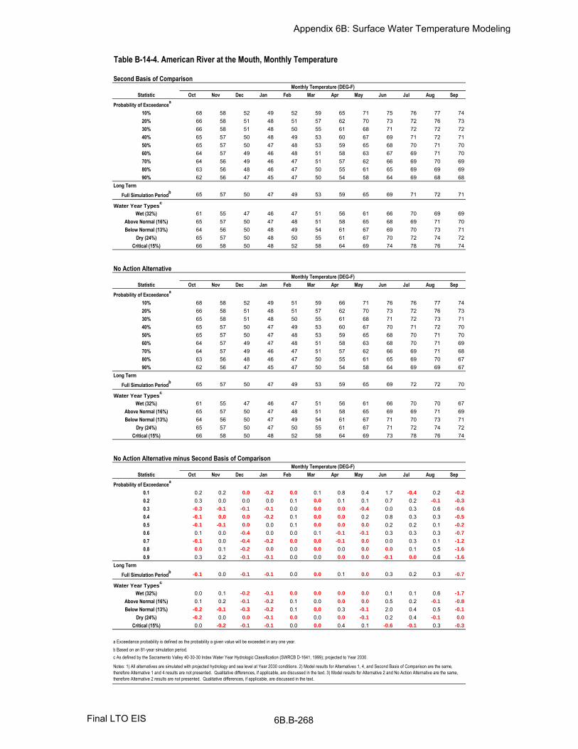
Oct Nov Dec Jan Feb Mar Apr May Jun Jul Aug Sep
10% 68 58 52 49 52 59 65 71 75 76 77 7420% 66 58 51 48 51 57 62 70 73 72 76 7330% 66 58 51 48 50 55 61 68 71 72 72 7240% 65 57 50 48 49 53 60 67 69 71 72 7150% 65 57 50 47 48 53 59 65 68 70 71 7060% 64 57 49 46 48 51 58 63 67 69 71 7070% 64 56 49 46 47 51 57 62 66 69 70 6980% 63 56 48 46 47 50 55 61 65 69 69 6990% 62 56 47 45 47 50 54 58 64 69 68 68
Full Simulation Periodb 65 57 50 47 49 53 59 65 69 71 72 71
Wet (32%) 61 55 47 46 47 51 56 61 66 70 69 69Above Normal (16%) 65 57 50 47 48 51 58 65 68 69 71 70Below Normal (13%) 64 56 50 48 49 54 61 67 69 70 73 71
Dry (24%) 65 57 50 48 50 55 61 67 70 72 74 72Critical (15%) 66 58 50 48 52 58 64 69 74 78 76 74
Oct Nov Dec Jan Feb Mar Apr May Jun Jul Aug Sep
10% 68 58 52 49 51 59 66 71 76 76 77 7420% 66 58 51 48 51 57 62 70 73 72 76 7330% 65 58 51 48 50 55 61 68 71 72 73 7140% 65 57 50 47 49 53 60 67 70 71 72 7050% 65 57 50 47 48 53 59 65 68 70 71 7060% 64 57 49 47 48 51 58 63 68 70 71 6970% 64 57 49 46 47 51 57 62 66 69 71 6880% 63 56 48 46 47 50 55 61 65 69 70 6790% 62 56 47 45 47 50 54 58 64 69 69 67
Full Simulation Periodb 65 57 50 47 49 53 59 65 69 72 72 70
Wet (32%) 61 55 47 46 47 51 56 61 66 70 70 67Above Normal (16%) 65 57 50 47 48 51 58 65 69 69 71 69Below Normal (13%) 64 56 50 47 49 54 61 67 71 70 73 71
Dry (24%) 65 57 50 47 50 55 61 67 71 72 74 72Critical (15%) 66 58 50 48 52 58 64 69 73 78 76 74
Oct Nov Dec Jan Feb Mar Apr May Jun Jul Aug Sep
0.1 0.2 0.2 0.0 -0.2 0.0 0.1 0.8 0.4 1.7 -0.4 0.2 -0.2
0.2 0.3 0.0 0.0 0.0 0.1 0.0 0.1 0.1 0.7 0.2 -0.1 -0.3
0.3 -0.3 -0.1 -0.1 -0.1 0.0 0.0 0.0 -0.4 0.0 0.3 0.6 -0.6
0.4 -0.1 0.0 0.0 -0.2 0.1 0.0 0.0 0.2 0.8 0.3 0.3 -0.5
0.5 -0.1 -0.1 0.0 0.0 0.1 0.0 0.0 0.0 0.2 0.2 0.1 -0.2
0.6 0.1 0.0 -0.4 0.0 0.0 0.1 -0.1 -0.1 0.3 0.3 0.3 -0.7
0.7 -0.1 0.0 -0.4 -0.2 0.0 0.0 -0.1 0.0 0.0 0.3 0.1 -1.2
0.8 0.0 0.1 -0.2 0.0 0.0 0.0 0.0 0.0 0.0 0.1 0.5 -1.6
0.9 0.3 0.2 -0.1 -0.1 0.0 0.0 0.0 0.0 -0.1 0.0 0.6 -1.6
Full Simulation Periodb
-0.1 0.0 -0.1 -0.1 0.0 0.0 0.1 0.0 0.3 0.2 0.3 -0.7
Wet (32%) 0.0 0.1 -0.2 -0.1 0.0 0.0 0.0 0.0 0.1 0.1 0.6 -1.7
Above Normal (16%) 0.1 0.2 -0.1 -0.2 0.1 0.0 0.0 0.0 0.5 0.2 -0.1 -0.8
Below Normal (13%) -0.2 -0.1 -0.3 -0.2 0.1 0.0 0.3 -0.1 2.0 0.4 0.5 -0.1
Dry (24%) -0.2 0.0 0.0 -0.1 0.0 0.0 0.0 -0.1 0.2 0.4 -0.1 0.0
Critical (15%) 0.0 -0.2 -0.1 -0.1 0.0 0.0 0.4 0.1 -0.6 -0.1 0.3 -0.3
a Exceedance probability is defined as the probability a given value will be exceeded in any one year.
b Based on an 81-year simulation period.
Probability of Exceedancea
Long Term
Water Year Typesc
c As defined by the Sacramento Valley 40-30-30 Index Water Year Hydrologic Classification (SWRCB D-1641, 1999); projected to Year 2030.
Notes: 1) All alternatives are simulated with projected hydrology and sea level at Year 2030 conditions. 2) Model results for Alternatives 1, 4, and Second Basis of Comparison are the same,
therefore Alternative 1 and 4 results are not presented. Qualitative differences, if applicable, are discussed in the text. 3) Model results for Alternative 2 and No Action Alternative are the same,
therefore Alternative 2 results are not presented. Qualitative differences, if applicable, are discussed in the text.
Probability of Exceedancea
Long Term
Water Year Typesc
No Action Alternative minus Second Basis of Comparison
Statistic
Monthly Temperature (DEG-F)
Long Term
Water Year Typesc
No Action Alternative
Statistic
Monthly Temperature (DEG-F)
Table B-14-4. American River at the Mouth, Monthly Temperature
Second Basis of Comparison
Statistic
Monthly Temperature (DEG-F)
Probability of Exceedancea
Appendix 6B: Surface Water Temperature Modeling
6B.B-268Final LTO EIS

Oct Nov Dec Jan Feb Mar Apr May Jun Jul Aug Sep
10% 68 58 52 49 52 59 65 71 75 76 77 7420% 66 58 51 48 51 57 62 70 73 72 76 7330% 66 58 51 48 50 55 61 68 71 72 72 7240% 65 57 50 48 49 53 60 67 69 71 72 7150% 65 57 50 47 48 53 59 65 68 70 71 7060% 64 57 49 46 48 51 58 63 67 69 71 7070% 64 56 49 46 47 51 57 62 66 69 70 6980% 63 56 48 46 47 50 55 61 65 69 69 6990% 62 56 47 45 47 50 54 58 64 69 68 68
Full Simulation Periodb 65 57 50 47 49 53 59 65 69 71 72 71
Wet (32%) 61 55 47 46 47 51 56 61 66 70 69 69Above Normal (16%) 65 57 50 47 48 51 58 65 68 69 71 70Below Normal (13%) 64 56 50 48 49 54 61 67 69 70 73 71
Dry (24%) 65 57 50 48 50 55 61 67 70 72 74 72Critical (15%) 66 58 50 48 52 58 64 69 74 78 76 74
Oct Nov Dec Jan Feb Mar Apr May Jun Jul Aug Sep
10% 68 59 52 49 52 59 66 71 76 76 77 7420% 66 58 51 48 51 57 62 70 72 72 75 7330% 66 58 51 48 50 55 61 68 71 72 73 7140% 65 57 50 48 49 53 60 67 70 71 72 7150% 65 57 50 47 48 53 59 65 68 70 72 7060% 64 57 50 47 48 51 58 63 67 70 71 7070% 64 56 49 46 47 51 57 62 66 69 70 6980% 63 56 48 46 47 50 55 61 65 69 69 6990% 62 56 47 45 47 50 54 58 64 68 68 68
Full Simulation Periodb 65 57 50 47 49 53 59 65 69 71 72 71
Wet (32%) 61 55 47 46 47 51 56 61 65 70 69 69Above Normal (16%) 65 57 50 47 48 51 58 65 68 69 71 70Below Normal (13%) 64 57 50 48 49 54 61 67 70 70 73 71
Dry (24%) 65 57 50 48 50 55 61 67 71 72 73 72Critical (15%) 66 58 50 48 52 58 64 69 74 78 76 74
Oct Nov Dec Jan Feb Mar Apr May Jun Jul Aug Sep
0.1 0.1 0.2 0.0 0.1 0.0 0.0 0.5 0.0 1.1 -0.4 0.3 0.0
0.2 0.0 0.1 0.0 0.1 -0.1 0.0 0.1 0.1 -0.4 0.4 -0.5 -0.2
0.3 -0.1 0.0 0.1 0.0 0.0 0.0 0.0 0.0 0.0 0.0 0.6 -0.2
0.4 -0.1 -0.1 -0.1 0.0 0.0 0.0 0.0 0.0 0.7 0.3 0.1 -0.1
0.5 -0.1 0.0 0.1 0.0 0.0 0.0 0.0 -0.3 -0.1 0.3 0.2 -0.1
0.6 0.1 0.0 0.1 0.1 0.0 0.0 0.0 -0.1 -0.5 0.2 0.2 -0.1
0.7 0.0 0.0 -0.2 0.0 0.0 0.0 -0.1 0.0 0.0 0.2 0.0 -0.1
0.8 0.0 0.0 0.0 0.0 0.0 0.0 0.0 0.0 0.0 0.0 -0.2 -0.1
0.9 0.0 0.3 0.0 0.0 0.0 0.0 0.0 0.0 0.0 -0.3 0.4 -0.7
Full Simulation Periodb
0.0 0.0 0.0 0.0 0.0 0.0 0.1 0.0 0.1 0.1 0.1 -0.1
Wet (32%) 0.0 0.0 0.0 0.0 0.0 0.0 0.0 0.0 -0.2 0.2 0.2 -0.1
Above Normal (16%) 0.1 0.1 0.0 0.0 0.0 0.0 0.0 0.0 -0.1 -0.1 0.2 0.1Below Normal (13%) 0.0 0.1 0.0 0.0 0.0 0.0 0.2 -0.2 1.3 0.2 -0.2 -0.3
Dry (24%) -0.1 0.0 0.1 0.0 0.0 0.0 0.0 0.0 0.0 0.4 -0.3 -0.1
Critical (15%) 0.0 -0.1 -0.1 0.0 0.0 -0.1 0.2 0.0 -0.2 -0.2 0.5 0.0
a Exceedance probability is defined as the probability a given value will be exceeded in any one year.
b Based on an 81-year simulation period.
Probability of Exceedancea
Long Term
Water Year Typesc
c As defined by the Sacramento Valley 40-30-30 Index Water Year Hydrologic Classification (SWRCB D-1641, 1999); projected to Year 2030.
Notes: 1) All alternatives are simulated with projected hydrology and sea level at Year 2030 conditions. 2) Model results for Alternatives 1, 4, and Second Basis of Comparison are the same,
therefore Alternative 1 and 4 results are not presented. Qualitative differences, if applicable, are discussed in the text. 3) Model results for Alternative 2 and No Action Alternative are the same,
therefore Alternative 2 results are not presented. Qualitative differences, if applicable, are discussed in the text.
Probability of Exceedancea
Long Term
Water Year Typesc
Alternative 3 minus Second Basis of Comparison
Statistic
Monthly Temperature (DEG-F)
Long Term
Water Year Typesc
Alternative 3
Statistic
Monthly Temperature (DEG-F)
Table B-14-5. American River at the Mouth, Monthly Temperature
Second Basis of Comparison
Statistic
Monthly Temperature (DEG-F)
Probability of Exceedancea
Appendix 6B: Surface Water Temperature Modeling
6B.B-269Final LTO EIS

Oct Nov Dec Jan Feb Mar Apr May Jun Jul Aug Sep
10% 68 58 52 49 52 59 65 71 75 76 77 7420% 66 58 51 48 51 57 62 70 73 72 76 7330% 66 58 51 48 50 55 61 68 71 72 72 7240% 65 57 50 48 49 53 60 67 69 71 72 7150% 65 57 50 47 48 53 59 65 68 70 71 7060% 64 57 49 46 48 51 58 63 67 69 71 7070% 64 56 49 46 47 51 57 62 66 69 70 6980% 63 56 48 46 47 50 55 61 65 69 69 6990% 62 56 47 45 47 50 54 58 64 69 68 68
Full Simulation Periodb 65 57 50 47 49 53 59 65 69 71 72 71
Wet (32%) 61 55 47 46 47 51 56 61 66 70 69 69Above Normal (16%) 65 57 50 47 48 51 58 65 68 69 71 70Below Normal (13%) 64 56 50 48 49 54 61 67 69 70 73 71
Dry (24%) 65 57 50 48 50 55 61 67 70 72 74 72Critical (15%) 66 58 50 48 52 58 64 69 74 78 76 74
Oct Nov Dec Jan Feb Mar Apr May Jun Jul Aug Sep
10% 68 58 52 49 51 59 66 71 77 76 77 7420% 66 58 51 48 51 57 63 70 73 72 75 7330% 65 58 51 48 50 55 61 68 71 71 73 7140% 65 57 50 47 49 53 60 67 70 71 72 7050% 65 57 50 47 48 53 59 65 68 70 71 7060% 64 57 49 47 48 51 58 63 68 70 71 6970% 64 57 49 46 47 51 56 62 66 69 71 6880% 63 56 48 45 47 50 55 61 65 69 70 6790% 62 56 47 45 47 50 54 58 64 68 69 67
Full Simulation Periodb 65 57 50 47 49 53 59 65 69 71 72 70
Wet (32%) 61 55 47 46 47 51 56 61 66 70 70 67Above Normal (16%) 65 57 50 47 48 51 58 65 69 69 71 69Below Normal (13%) 64 56 50 47 49 54 61 67 71 70 74 71
Dry (24%) 65 57 50 47 50 55 61 67 71 72 74 72Critical (15%) 66 58 50 48 52 58 65 70 73 77 76 74
Oct Nov Dec Jan Feb Mar Apr May Jun Jul Aug Sep
0.1 0.1 0.1 0.0 -0.2 0.0 0.2 0.9 0.4 2.0 -0.5 0.2 0.0
0.2 0.3 0.0 0.0 0.0 0.1 0.0 0.6 0.4 0.5 0.1 -0.2 -0.3
0.3 -0.3 -0.1 -0.1 -0.1 0.1 0.0 0.0 -0.1 0.0 0.0 0.5 -0.4
0.4 -0.1 -0.1 0.0 -0.2 0.1 0.0 0.0 0.2 0.7 0.0 0.1 -0.5
0.5 -0.2 -0.1 0.0 0.0 0.1 0.0 0.0 0.0 0.2 0.1 0.1 -0.3
0.6 0.0 0.0 -0.3 0.0 0.0 0.0 -0.1 0.0 0.2 0.2 0.3 -0.7
0.7 -0.2 0.1 -0.4 -0.2 0.0 0.0 -0.1 0.0 -0.1 0.2 0.1 -1.2
0.8 0.2 0.0 -0.2 -0.1 0.0 0.0 0.0 0.0 0.0 0.0 0.8 -1.6
0.9 0.4 0.2 -0.1 -0.1 0.0 0.0 0.0 0.0 0.0 -0.1 0.7 -1.6
Full Simulation Periodb
-0.1 0.0 -0.2 -0.1 0.0 0.0 0.1 0.1 0.3 0.0 0.2 -0.6
Wet (32%) 0.0 0.0 -0.2 -0.1 0.0 0.0 0.0 0.0 0.1 -0.1 0.8 -1.7
Above Normal (16%) 0.1 0.0 -0.1 -0.2 0.1 0.0 0.0 0.0 0.5 0.2 -0.1 -0.8
Below Normal (13%) -0.2 0.0 -0.4 -0.3 0.0 0.0 0.4 0.0 2.1 0.3 0.6 0.0
Dry (24%) -0.2 0.0 0.0 -0.1 0.0 0.0 0.0 0.2 0.3 0.1 -0.2 0.0
Critical (15%) 0.0 -0.2 -0.1 -0.1 0.0 0.0 0.6 0.2 -1.1 -0.5 -0.2 0.3
a Exceedance probability is defined as the probability a given value will be exceeded in any one year.
b Based on an 81-year simulation period.
Probability of Exceedancea
Long Term
Water Year Typesc
c As defined by the Sacramento Valley 40-30-30 Index Water Year Hydrologic Classification (SWRCB D-1641, 1999); projected to Year 2030.
Notes: 1) All alternatives are simulated with projected hydrology and sea level at Year 2030 conditions. 2) Model results for Alternatives 1, 4, and Second Basis of Comparison are the same,
therefore Alternative 1 and 4 results are not presented. Qualitative differences, if applicable, are discussed in the text. 3) Model results for Alternative 2 and No Action Alternative are the same,
therefore Alternative 2 results are not presented. Qualitative differences, if applicable, are discussed in the text.
Probability of Exceedancea
Long Term
Water Year Typesc
Alternative 5 minus Second Basis of Comparison
Statistic
Monthly Temperature (DEG-F)
Long Term
Water Year Typesc
Alternative 5
Statistic
Monthly Temperature (DEG-F)
Table B-14-6. American River at the Mouth, Monthly Temperature
Second Basis of Comparison
Statistic
Monthly Temperature (DEG-F)
Probability of Exceedancea
Appendix 6B: Surface Water Temperature Modeling
6B.B-270Final LTO EIS

B.15. Stanislaus River below New Melones Temperature
Appendix 6B: Surface Water Temperature Modeling
6B.B-271Final LTO EIS

Figure B-15-1. Stanislaus River below New Melones Reservoir, October
Notes: 1) Exceedance probability is defined as the probability a given value will be exceeded in any one year. 2) All alternatives are simulated with projected hydrology and
sea level at Year 2030 conditions. 3) Model results for Alternatives 1, 4, and Second Basis of Comparison are the same, therefore Alternatives 1 and 4 results are not
presented. Qualitative differences, if applicable, are discussed in the text. 4) Model results for Alternative 2 and No Action Alternative are the same, therefore Alternative 2
results are not presented. Qualitative differences, if applicable, are discussed in the text.
44
46
48
50
52
54
56
58
60
62
64
66
68
70
0%10%20%30%40%50%60%70%80%90%100%
Exceedance Probability
No Action Alternative & Alternative 2 Second Basis of Comparison, Alternative 1, & Alternative 4
Alternative 3 Alternative 5
Mon
thly
Tem
pera
ture
(DE
G-F
)
Appendix 6B: Surface Water Temperature Modeling
6B.B-272Final LTO EIS
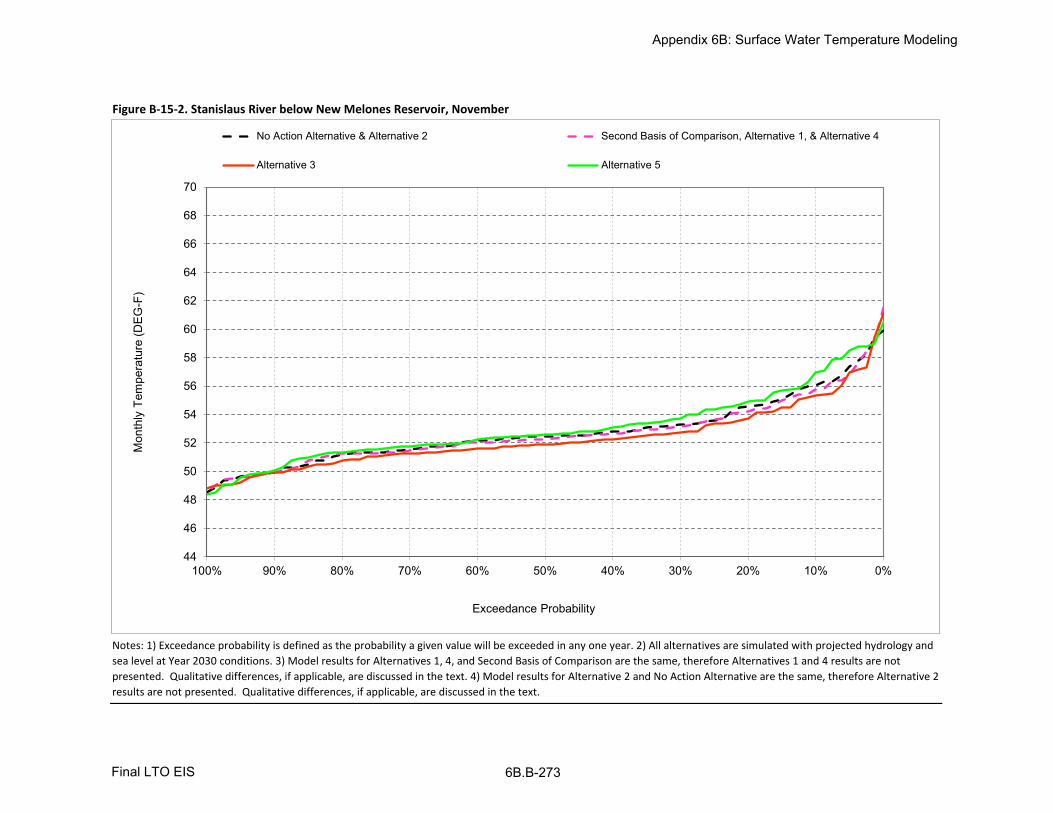
Figure B-15-2. Stanislaus River below New Melones Reservoir, November
Notes: 1) Exceedance probability is defined as the probability a given value will be exceeded in any one year. 2) All alternatives are simulated with projected hydrology and
sea level at Year 2030 conditions. 3) Model results for Alternatives 1, 4, and Second Basis of Comparison are the same, therefore Alternatives 1 and 4 results are not
presented. Qualitative differences, if applicable, are discussed in the text. 4) Model results for Alternative 2 and No Action Alternative are the same, therefore Alternative 2
results are not presented. Qualitative differences, if applicable, are discussed in the text.
44
46
48
50
52
54
56
58
60
62
64
66
68
70
0%10%20%30%40%50%60%70%80%90%100%
Exceedance Probability
No Action Alternative & Alternative 2 Second Basis of Comparison, Alternative 1, & Alternative 4
Alternative 3 Alternative 5
Mon
thly
Tem
pera
ture
(DE
G-F
)
Appendix 6B: Surface Water Temperature Modeling
6B.B-273Final LTO EIS

Figure B-15-3. Stanislaus River below New Melones Reservoir, December
Notes: 1) Exceedance probability is defined as the probability a given value will be exceeded in any one year. 2) All alternatives are simulated with projected hydrology and
sea level at Year 2030 conditions. 3) Model results for Alternatives 1, 4, and Second Basis of Comparison are the same, therefore Alternatives 1 and 4 results are not
presented. Qualitative differences, if applicable, are discussed in the text. 4) Model results for Alternative 2 and No Action Alternative are the same, therefore Alternative 2
results are not presented. Qualitative differences, if applicable, are discussed in the text.
44
46
48
50
52
54
56
58
60
62
64
66
68
70
0%10%20%30%40%50%60%70%80%90%100%
Exceedance Probability
No Action Alternative & Alternative 2 Second Basis of Comparison, Alternative 1, & Alternative 4
Alternative 3 Alternative 5
Mon
thly
Tem
pera
ture
(DE
G-F
)
Appendix 6B: Surface Water Temperature Modeling
6B.B-274Final LTO EIS

Figure B-15-4. Stanislaus River below New Melones Reservoir, January
Notes: 1) Exceedance probability is defined as the probability a given value will be exceeded in any one year. 2) All alternatives are simulated with projected hydrology and
sea level at Year 2030 conditions. 3) Model results for Alternatives 1, 4, and Second Basis of Comparison are the same, therefore Alternatives 1 and 4 results are not
presented. Qualitative differences, if applicable, are discussed in the text. 4) Model results for Alternative 2 and No Action Alternative are the same, therefore Alternative 2
results are not presented. Qualitative differences, if applicable, are discussed in the text.
44
46
48
50
52
54
56
58
60
62
64
66
68
70
0%10%20%30%40%50%60%70%80%90%100%
Exceedance Probability
No Action Alternative & Alternative 2 Second Basis of Comparison, Alternative 1, & Alternative 4
Alternative 3 Alternative 5
Mon
thly
Tem
pera
ture
(DE
G-F
)
Appendix 6B: Surface Water Temperature Modeling
6B.B-275Final LTO EIS
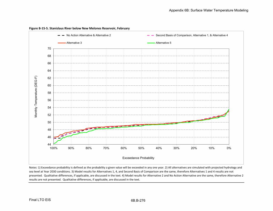
Figure B-15-5. Stanislaus River below New Melones Reservoir, February
Notes: 1) Exceedance probability is defined as the probability a given value will be exceeded in any one year. 2) All alternatives are simulated with projected hydrology and
sea level at Year 2030 conditions. 3) Model results for Alternatives 1, 4, and Second Basis of Comparison are the same, therefore Alternatives 1 and 4 results are not
presented. Qualitative differences, if applicable, are discussed in the text. 4) Model results for Alternative 2 and No Action Alternative are the same, therefore Alternative 2
results are not presented. Qualitative differences, if applicable, are discussed in the text.
44
46
48
50
52
54
56
58
60
62
64
66
68
70
0%10%20%30%40%50%60%70%80%90%100%
Exceedance Probability
No Action Alternative & Alternative 2 Second Basis of Comparison, Alternative 1, & Alternative 4
Alternative 3 Alternative 5
Mon
thly
Tem
pera
ture
(DE
G-F
)
Appendix 6B: Surface Water Temperature Modeling
6B.B-276Final LTO EIS

Figure B-15-6. Stanislaus River below New Melones Reservoir, March
Notes: 1) Exceedance probability is defined as the probability a given value will be exceeded in any one year. 2) All alternatives are simulated with projected hydrology and
sea level at Year 2030 conditions. 3) Model results for Alternatives 1, 4, and Second Basis of Comparison are the same, therefore Alternatives 1 and 4 results are not
presented. Qualitative differences, if applicable, are discussed in the text. 4) Model results for Alternative 2 and No Action Alternative are the same, therefore Alternative 2
results are not presented. Qualitative differences, if applicable, are discussed in the text.
44
46
48
50
52
54
56
58
60
62
64
66
68
70
0%10%20%30%40%50%60%70%80%90%100%
Exceedance Probability
No Action Alternative & Alternative 2 Second Basis of Comparison, Alternative 1, & Alternative 4
Alternative 3 Alternative 5
Mon
thly
Tem
pera
ture
(DE
G-F
)
Appendix 6B: Surface Water Temperature Modeling
6B.B-277Final LTO EIS

Figure B-15-7. Stanislaus River below New Melones Reservoir, April
Notes: 1) Exceedance probability is defined as the probability a given value will be exceeded in any one year. 2) All alternatives are simulated with projected hydrology and
sea level at Year 2030 conditions. 3) Model results for Alternatives 1, 4, and Second Basis of Comparison are the same, therefore Alternatives 1 and 4 results are not
presented. Qualitative differences, if applicable, are discussed in the text. 4) Model results for Alternative 2 and No Action Alternative are the same, therefore Alternative 2
results are not presented. Qualitative differences, if applicable, are discussed in the text.
44
46
48
50
52
54
56
58
60
62
64
66
68
70
0%10%20%30%40%50%60%70%80%90%100%
Exceedance Probability
No Action Alternative & Alternative 2 Second Basis of Comparison, Alternative 1, & Alternative 4
Alternative 3 Alternative 5
Mon
thly
Tem
pera
ture
(DE
G-F
)
Appendix 6B: Surface Water Temperature Modeling
6B.B-278Final LTO EIS

Figure B-15-8. Stanislaus River below New Melones Reservoir, May
Notes: 1) Exceedance probability is defined as the probability a given value will be exceeded in any one year. 2) All alternatives are simulated with projected hydrology and
sea level at Year 2030 conditions. 3) Model results for Alternatives 1, 4, and Second Basis of Comparison are the same, therefore Alternatives 1 and 4 results are not
presented. Qualitative differences, if applicable, are discussed in the text. 4) Model results for Alternative 2 and No Action Alternative are the same, therefore Alternative 2
results are not presented. Qualitative differences, if applicable, are discussed in the text.
44
46
48
50
52
54
56
58
60
62
64
66
68
70
0%10%20%30%40%50%60%70%80%90%100%
Exceedance Probability
No Action Alternative & Alternative 2 Second Basis of Comparison, Alternative 1, & Alternative 4
Alternative 3 Alternative 5
Mon
thly
Tem
pera
ture
(DE
G-F
)
Appendix 6B: Surface Water Temperature Modeling
6B.B-279Final LTO EIS

Figure B-15-9. Stanislaus River below New Melones Reservoir, June
Notes: 1) Exceedance probability is defined as the probability a given value will be exceeded in any one year. 2) All alternatives are simulated with projected hydrology and
sea level at Year 2030 conditions. 3) Model results for Alternatives 1, 4, and Second Basis of Comparison are the same, therefore Alternatives 1 and 4 results are not
presented. Qualitative differences, if applicable, are discussed in the text. 4) Model results for Alternative 2 and No Action Alternative are the same, therefore Alternative 2
results are not presented. Qualitative differences, if applicable, are discussed in the text.
44
46
48
50
52
54
56
58
60
62
64
66
68
70
0%10%20%30%40%50%60%70%80%90%100%
Exceedance Probability
No Action Alternative & Alternative 2 Second Basis of Comparison, Alternative 1, & Alternative 4
Alternative 3 Alternative 5
Mon
thly
Tem
pera
ture
(DE
G-F
)
Appendix 6B: Surface Water Temperature Modeling
6B.B-280Final LTO EIS

Figure B-15-10. Stanislaus River below New Melones Reservoir, July
Notes: 1) Exceedance probability is defined as the probability a given value will be exceeded in any one year. 2) All alternatives are simulated with projected hydrology and
sea level at Year 2030 conditions. 3) Model results for Alternatives 1, 4, and Second Basis of Comparison are the same, therefore Alternatives 1 and 4 results are not
presented. Qualitative differences, if applicable, are discussed in the text. 4) Model results for Alternative 2 and No Action Alternative are the same, therefore Alternative 2
results are not presented. Qualitative differences, if applicable, are discussed in the text.
44
46
48
50
52
54
56
58
60
62
64
66
68
70
0%10%20%30%40%50%60%70%80%90%100%
Exceedance Probability
No Action Alternative & Alternative 2 Second Basis of Comparison, Alternative 1, & Alternative 4
Alternative 3 Alternative 5
Mon
thly
Tem
pera
ture
(DE
G-F
)
Appendix 6B: Surface Water Temperature Modeling
6B.B-281Final LTO EIS

Figure B-15-11. Stanislaus River below New Melones Reservoir, August
Notes: 1) Exceedance probability is defined as the probability a given value will be exceeded in any one year. 2) All alternatives are simulated with projected hydrology and
sea level at Year 2030 conditions. 3) Model results for Alternatives 1, 4, and Second Basis of Comparison are the same, therefore Alternatives 1 and 4 results are not
presented. Qualitative differences, if applicable, are discussed in the text. 4) Model results for Alternative 2 and No Action Alternative are the same, therefore Alternative 2
results are not presented. Qualitative differences, if applicable, are discussed in the text.
44
46
48
50
52
54
56
58
60
62
64
66
68
70
0%10%20%30%40%50%60%70%80%90%100%
Exceedance Probability
No Action Alternative & Alternative 2 Second Basis of Comparison, Alternative 1, & Alternative 4
Alternative 3 Alternative 5
Mon
thly
Tem
pera
ture
(DE
G-F
)
Appendix 6B: Surface Water Temperature Modeling
6B.B-282Final LTO EIS

Figure B-15-12. Stanislaus River below New Melones Reservoir, September
Notes: 1) Exceedance probability is defined as the probability a given value will be exceeded in any one year. 2) All alternatives are simulated with projected hydrology and
sea level at Year 2030 conditions. 3) Model results for Alternatives 1, 4, and Second Basis of Comparison are the same, therefore Alternatives 1 and 4 results are not
presented. Qualitative differences, if applicable, are discussed in the text. 4) Model results for Alternative 2 and No Action Alternative are the same, therefore Alternative 2
results are not presented. Qualitative differences, if applicable, are discussed in the text.
44
46
48
50
52
54
56
58
60
62
64
66
68
70
0%10%20%30%40%50%60%70%80%90%100%
Exceedance Probability
No Action Alternative & Alternative 2 Second Basis of Comparison, Alternative 1, & Alternative 4
Alternative 3 Alternative 5
Mon
thly
Tem
pera
ture
(DE
G-F
)
Appendix 6B: Surface Water Temperature Modeling
6B.B-283Final LTO EIS

Oct Nov Dec Jan Feb Mar Apr May Jun Jul Aug Sep
10% 59 56 54 52 51 51 51 52 53 54 55 5720% 56 55 53 51 50 50 50 51 52 53 53 5430% 53 53 52 51 50 49 50 51 51 52 53 5340% 53 53 52 51 49 49 50 50 51 51 52 5350% 52 52 52 50 49 49 49 50 50 51 52 5260% 52 52 51 50 49 49 49 49 50 50 51 5170% 51 52 51 50 49 48 48 49 49 50 50 5180% 51 51 50 49 48 48 48 48 49 50 50 5190% 50 50 50 48 47 47 47 47 48 48 49 49
Full Simulation Periodb 53 53 52 50 49 49 49 50 51 51 52 53
Wet (32%) 50 50 49 49 48 48 48 48 49 49 50 50Above Normal (16%) 53 53 52 50 49 48 49 49 50 50 51 52Below Normal (13%) 53 52 52 51 49 49 49 50 50 51 52 52
Dry (24%) 53 53 52 51 50 50 50 50 51 52 53 54Critical (15%) 57 54 52 50 50 50 51 53 55 56 57 60
Oct Nov Dec Jan Feb Mar Apr May Jun Jul Aug Sep
10% 58 56 54 52 51 51 51 52 52 54 55 5720% 54 54 53 51 50 50 50 51 52 52 53 5430% 53 53 52 51 50 50 50 50 51 52 52 5340% 53 53 52 51 49 49 50 50 51 51 52 5250% 52 52 52 50 49 49 49 50 50 51 52 5260% 52 52 51 50 49 49 49 49 50 50 51 5170% 51 52 51 50 49 48 48 49 49 50 50 5180% 51 51 50 49 48 48 48 48 49 50 50 5190% 50 50 50 48 47 47 47 47 48 48 49 49
Full Simulation Periodb 53 53 52 50 49 49 49 50 50 51 52 53
Wet (32%) 50 50 49 49 48 48 48 48 49 49 50 50Above Normal (16%) 53 53 52 50 49 48 49 49 50 50 51 52Below Normal (13%) 52 52 51 51 49 49 49 50 50 51 52 52
Dry (24%) 53 53 52 51 50 50 50 50 51 52 53 54Critical (15%) 57 55 53 51 50 50 51 53 53 56 57 58
Oct Nov Dec Jan Feb Mar Apr May Jun Jul Aug Sep
0.1 -0.7 -0.3 0.0 0.0 0.3 0.1 0.0 0.0 -0.1 -0.1 0.1 -0.9
0.2 -1.4 -0.4 0.0 -0.1 0.1 0.1 0.0 0.0 0.0 -0.1 -0.1 -0.9
0.3 -0.3 -0.1 0.0 0.0 0.1 0.1 0.1 0.0 0.0 -0.2 -0.1 -0.1
0.4 -0.4 -0.1 0.1 0.1 0.1 0.0 0.0 0.0 0.0 0.0 0.0 -0.2
0.5 -0.3 -0.2 0.0 0.1 0.1 0.0 0.0 0.0 0.0 -0.1 0.0 -0.2
0.6 -0.2 -0.1 0.0 0.1 0.1 0.0 0.0 0.0 0.0 0.0 0.0 0.0
0.7 -0.2 -0.1 0.0 0.0 0.0 0.0 0.1 0.0 0.1 0.0 0.0 -0.1
0.8 -0.1 0.0 0.0 0.1 0.2 0.1 0.1 0.1 0.0 0.0 0.1 -0.1
0.9 -0.3 0.0 0.0 0.2 0.0 0.0 0.0 0.0 0.1 0.0 -0.2 0.1
Full Simulation Periodb
-0.3 -0.1 0.0 0.1 0.1 0.0 0.0 0.0 -0.2 0.1 -0.1 -0.4
Wet (32%) -0.3 -0.2 0.0 0.1 0.1 -0.1 0.1 0.0 0.1 0.0 0.0 0.0
Above Normal (16%) -0.4 -0.3 -0.1 0.0 0.0 0.1 0.0 0.0 0.0 0.0 0.0 -0.1
Below Normal (13%) -0.6 -0.4 -0.1 0.1 0.1 0.1 0.0 0.0 -0.1 -0.1 -0.2 -0.3
Dry (24%) -0.3 -0.3 -0.1 0.0 0.1 0.0 0.0 0.0 0.0 -0.1 -0.2 -0.3
Critical (15%) -0.1 1.0 0.3 0.3 0.3 0.2 -0.3 0.2 -1.4 0.6 -0.1 -2.1
a Exceedance probability is defined as the probability a given value will be exceeded in any one year.
b Based on an 81-year simulation period.
Probability of Exceedancea
Long Term
Water Year Typesc
c As defined by the Sacramento Valley 40-30-30 Index Water Year Hydrologic Classification (SWRCB D-1641, 1999); projected to Year 2030.
Notes: 1) All alternatives are simulated with projected hydrology and sea level at Year 2030 conditions. 2) Model results for Alternatives 1, 4, and Second Basis of Comparison are the same,
therefore Second Basis of Comparison and Alternative 4 results are not presented. Qualitative differences, if applicable, are discussed in the text. 3) Model results for Alternative 2 and No Action
Alternative are the same, therefore Alternative 2 results are not presented. Qualitative differences, if applicable, are discussed in the text.
Probability of Exceedancea
Long Term
Water Year Typesc
Alternative 1 minus No Action Alternative
Statistic
Monthly Temperature (DEG-F)
Long Term
Water Year Typesc
Alternative 1
Statistic
Monthly Temperature (DEG-F)
Table B-15-1. Stanislaus River below New Melones Reservoir, Monthly Temperature
No Action Alternative
Statistic
Monthly Temperature (DEG-F)
Probability of Exceedancea
Appendix 6B: Surface Water Temperature Modeling
6B-.B-284Final LTO EIS

Oct Nov Dec Jan Feb Mar Apr May Jun Jul Aug Sep
10% 59 56 54 52 51 51 51 52 53 54 55 5720% 56 55 53 51 50 50 50 51 52 53 53 5430% 53 53 52 51 50 49 50 51 51 52 53 5340% 53 53 52 51 49 49 50 50 51 51 52 5350% 52 52 52 50 49 49 49 50 50 51 52 5260% 52 52 51 50 49 49 49 49 50 50 51 5170% 51 52 51 50 49 48 48 49 49 50 50 5180% 51 51 50 49 48 48 48 48 49 50 50 5190% 50 50 50 48 47 47 47 47 48 48 49 49
Full Simulation Periodb 53 53 52 50 49 49 49 50 51 51 52 53
Wet (32%) 50 50 49 49 48 48 48 48 49 49 50 50Above Normal (16%) 53 53 52 50 49 48 49 49 50 50 51 52Below Normal (13%) 53 52 52 51 49 49 49 50 50 51 52 52
Dry (24%) 53 53 52 51 50 50 50 50 51 52 53 54Critical (15%) 57 54 52 50 50 50 51 53 55 56 57 60
Oct Nov Dec Jan Feb Mar Apr May Jun Jul Aug Sep
10% 56 55 53 52 51 51 51 52 52 53 54 5520% 54 54 53 51 50 50 50 51 52 52 53 5330% 53 53 52 51 50 50 50 50 51 51 52 5340% 52 52 52 51 50 49 50 50 51 51 52 5250% 52 52 51 50 49 49 49 50 50 51 51 5160% 51 52 51 50 49 49 49 49 50 50 51 5170% 51 51 51 50 49 49 49 49 49 50 50 5180% 51 51 51 49 48 48 48 48 49 49 50 5090% 50 50 50 48 47 47 47 48 48 49 49 49
Full Simulation Periodb 52 52 52 50 49 49 49 50 50 51 52 52
Wet (32%) 49 50 49 49 48 48 48 49 49 49 50 50Above Normal (16%) 52 52 51 50 49 49 49 49 50 50 51 51Below Normal (13%) 52 51 51 50 49 49 49 50 50 51 51 52
Dry (24%) 52 52 52 51 50 50 50 50 51 51 52 53Critical (15%) 56 55 53 51 50 50 51 52 54 56 56 57
Oct Nov Dec Jan Feb Mar Apr May Jun Jul Aug Sep
0.1 -3.2 -0.7 -0.4 0.1 0.0 0.1 0.1 0.0 -0.4 -0.7 -1.4 -2.6
0.2 -2.0 -0.8 -0.2 0.0 0.0 0.2 0.2 -0.2 -0.2 -0.4 -0.3 -1.1
0.3 -0.8 -0.5 -0.2 0.0 0.2 0.1 0.1 -0.1 -0.2 -0.4 -0.5 -0.5
0.4 -0.9 -0.5 -0.2 0.0 0.1 0.1 0.0 -0.1 -0.3 -0.2 -0.3 -0.6
0.5 -0.7 -0.6 -0.1 0.1 0.2 0.1 0.0 -0.1 -0.3 -0.6 -0.5 -0.5
0.6 -0.7 -0.6 -0.1 0.1 0.1 0.1 0.1 0.0 0.0 -0.2 -0.2 -0.3
0.7 -0.3 -0.3 0.0 0.1 0.1 0.4 0.4 0.1 0.1 -0.1 -0.1 -0.2
0.8 -0.5 -0.4 0.2 0.1 0.3 0.5 0.2 0.1 0.0 -0.3 -0.3 -0.3
0.9 -0.3 0.0 0.2 0.1 0.4 0.3 0.3 0.4 0.5 0.1 0.0 0.2
Full Simulation Periodb
-0.9 -0.4 -0.1 0.1 0.2 0.2 0.1 -0.1 -0.2 -0.2 -0.5 -1.0
Wet (32%) -0.6 -0.5 -0.1 0.0 0.2 0.1 0.2 0.1 0.1 0.0 -0.1 -0.1
Above Normal (16%) -1.0 -0.8 -0.3 0.0 0.2 0.2 0.2 0.1 0.0 -0.2 -0.4 -0.5
Below Normal (13%) -1.3 -1.0 -0.5 -0.1 0.1 0.2 0.1 0.0 -0.2 -0.3 -0.5 -0.6
Dry (24%) -0.7 -0.5 -0.2 -0.1 0.0 0.1 0.1 -0.1 -0.3 -0.5 -0.8 -1.2
Critical (15%) -1.6 0.7 0.5 0.8 0.8 0.5 -0.2 -1.2 -1.1 -0.1 -1.1 -3.6
a Exceedance probability is defined as the probability a given value will be exceeded in any one year.
b Based on an 81-year simulation period.
Probability of Exceedancea
Long Term
Water Year Typesc
c As defined by the Sacramento Valley 40-30-30 Index Water Year Hydrologic Classification (SWRCB D-1641, 1999); projected to Year 2030.
Notes: 1) All alternatives are simulated with projected hydrology and sea level at Year 2030 conditions. 2) Model results for Alternatives 1, 4, and Second Basis of Comparison are the same,
therefore Alternative 1 and 4 results are not presented. Qualitative differences, if applicable, are discussed in the text. 3) Model results for Alternative 2 and No Action Alternative are the same,
therefore Alternative 2 results are not presented. Qualitative differences, if applicable, are discussed in the text.
Probability of Exceedancea
Long Term
Water Year Typesc
Alternative 3 minus No Action Alternative
Statistic
Monthly Temperature (DEG-F)
Long Term
Water Year Typesc
Alternative 3
Statistic
Monthly Temperature (DEG-F)
Table B-15-2. Stanislaus River below New Melones Reservoir, Monthly Temperature
No Action Alternative
Statistic
Monthly Temperature (DEG-F)
Probability of Exceedancea
Appendix 6B: Surface Water Temperature Modeling
6B.B-285Final LTO EIS

Oct Nov Dec Jan Feb Mar Apr May Jun Jul Aug Sep
10% 59 56 54 52 51 51 51 52 53 54 55 5720% 56 55 53 51 50 50 50 51 52 53 53 5430% 53 53 52 51 50 49 50 51 51 52 53 5340% 53 53 52 51 49 49 50 50 51 51 52 5350% 52 52 52 50 49 49 49 50 50 51 52 5260% 52 52 51 50 49 49 49 49 50 50 51 5170% 51 52 51 50 49 48 48 49 49 50 50 5180% 51 51 50 49 48 48 48 48 49 50 50 5190% 50 50 50 48 47 47 47 47 48 48 49 49
Full Simulation Periodb 53 53 52 50 49 49 49 50 51 51 52 53
Wet (32%) 50 50 49 49 48 48 48 48 49 49 50 50Above Normal (16%) 53 53 52 50 49 48 49 49 50 50 51 52Below Normal (13%) 53 52 52 51 49 49 49 50 50 51 52 52
Dry (24%) 53 53 52 51 50 50 50 50 51 52 53 54Critical (15%) 57 54 52 50 50 50 51 53 55 56 57 60
Oct Nov Dec Jan Feb Mar Apr May Jun Jul Aug Sep
10% 61 57 54 52 51 51 51 52 53 55 60 6320% 57 55 53 51 50 50 50 51 52 53 54 5630% 54 54 52 51 50 49 50 51 51 52 53 5440% 53 53 52 50 49 49 50 50 51 52 52 5350% 53 53 52 50 49 49 49 50 50 51 52 5260% 52 52 51 50 49 49 49 49 50 50 51 5270% 52 52 51 49 48 48 49 49 49 50 51 5180% 51 51 50 49 47 47 48 48 49 50 50 5190% 50 50 50 48 46 46 47 47 47 48 49 50
Full Simulation Periodb 54 53 52 50 49 49 49 50 50 52 53 54
Wet (32%) 51 50 49 49 48 48 48 48 49 49 50 50Above Normal (16%) 54 53 52 50 49 48 48 49 50 50 51 52Below Normal (13%) 53 52 51 50 49 49 49 50 51 52 53 53
Dry (24%) 54 53 52 51 50 49 50 51 51 53 54 56Critical (15%) 58 55 52 50 49 50 52 54 53 56 58 61
Oct Nov Dec Jan Feb Mar Apr May Jun Jul Aug Sep
0.1 1.9 0.9 0.3 -0.2 -0.1 0.0 0.2 0.6 0.5 1.8 4.7 5.70.2 1.1 0.4 0.1 -0.1 0.0 0.1 0.2 0.3 0.2 0.8 1.4 1.60.3 1.0 0.5 -0.1 0.0 -0.1 0.0 0.1 0.2 0.2 0.4 0.5 0.80.4 0.3 0.3 0.0 -0.2 0.0 0.0 0.1 0.0 -0.1 0.1 0.2 0.30.5 0.1 0.1 0.0 0.0 -0.2 0.0 0.0 0.1 -0.1 0.1 0.1 0.10.6 0.1 0.1 -0.1 -0.2 -0.2 -0.1 0.0 0.0 -0.1 0.0 0.0 0.10.7 0.2 0.2 0.0 -0.2 -0.3 -0.1 0.2 0.0 -0.1 0.0 0.1 0.10.8 0.0 0.1 -0.1 -0.3 -0.7 -0.2 -0.3 -0.3 -0.4 -0.1 0.1 0.0
0.9 0.0 0.1 -0.3 -0.5 -0.6 -0.5 -0.2 -0.1 -0.1 0.0 0.0 0.3
Full Simulation Periodb 0.6 0.3 0.0 -0.2 -0.3 -0.1 0.0 0.2 -0.2 0.4 0.7 0.7
Wet (32%) 0.7 0.2 -0.1 -0.2 -0.2 -0.2 -0.2 -0.1 -0.1 0.0 0.1 0.1Above Normal (16%) 0.5 0.4 0.1 0.0 -0.1 -0.1 -0.1 0.0 0.1 0.1 0.2 0.3Below Normal (13%) 0.3 -0.2 -0.3 -0.4 -0.3 -0.2 0.0 0.2 0.3 0.5 0.7 0.9
Dry (24%) 0.7 0.6 0.3 -0.1 -0.1 -0.1 0.0 0.1 0.3 0.8 1.6 1.9Critical (15%) 0.5 0.6 -0.1 -0.7 -0.7 0.2 0.8 1.1 -2.1 0.7 0.8 0.3
a Exceedance probability is defined as the probability a given value will be exceeded in any one year.
b Based on an 81-year simulation period.
Probability of Exceedancea
Long Term
Water Year Typesc
c As defined by the Sacramento Valley 40-30-30 Index Water Year Hydrologic Classification (SWRCB D-1641, 1999); projected to Year 2030.
Notes: 1) All alternatives are simulated with projected hydrology and sea level at Year 2030 conditions. 2) Model results for Alternatives 1, 4, and Second Basis of Comparison are the same,
therefore Alternative 1 and 4 results are not presented. Qualitative differences, if applicable, are discussed in the text. 3) Model results for Alternative 2 and No Action Alternative are the same,
therefore Alternative 2 results are not presented. Qualitative differences, if applicable, are discussed in the text.
Probability of Exceedancea
Long Term
Water Year Typesc
Alternative 5 minus No Action Alternative
Statistic
Monthly Temperature (DEG-F)
Long Term
Water Year Typesc
Alternative 5
Statistic
Monthly Temperature (DEG-F)
Table B-15-3. Stanislaus River below New Melones Reservoir, Monthly Temperature
No Action Alternative
Statistic
Monthly Temperature (DEG-F)
Probability of Exceedancea
Appendix 6B: Surface Water Temperature Modeling
6B.B-286Final LTO EIS

Oct Nov Dec Jan Feb Mar Apr May Jun Jul Aug Sep
10% 58 56 54 52 51 51 51 52 52 54 55 5720% 54 54 53 51 50 50 50 51 52 52 53 5430% 53 53 52 51 50 50 50 50 51 52 52 5340% 53 53 52 51 49 49 50 50 51 51 52 5250% 52 52 52 50 49 49 49 50 50 51 52 5260% 52 52 51 50 49 49 49 49 50 50 51 5170% 51 52 51 50 49 48 48 49 49 50 50 5180% 51 51 50 49 48 48 48 48 49 50 50 5190% 50 50 50 48 47 47 47 47 48 48 49 49
Full Simulation Periodb 53 53 52 50 49 49 49 50 50 51 52 53
Wet (32%) 50 50 49 49 48 48 48 48 49 49 50 50Above Normal (16%) 53 53 52 50 49 48 49 49 50 50 51 52Below Normal (13%) 52 52 51 51 49 49 49 50 50 51 52 52
Dry (24%) 53 53 52 51 50 50 50 50 51 52 53 54Critical (15%) 57 55 53 51 50 50 51 53 53 56 57 58
Oct Nov Dec Jan Feb Mar Apr May Jun Jul Aug Sep
10% 59 56 54 52 51 51 51 52 53 54 55 5720% 56 55 53 51 50 50 50 51 52 53 53 5430% 53 53 52 51 50 49 50 51 51 52 53 5340% 53 53 52 51 49 49 50 50 51 51 52 5350% 52 52 52 50 49 49 49 50 50 51 52 5260% 52 52 51 50 49 49 49 49 50 50 51 5170% 51 52 51 50 49 48 48 49 49 50 50 5180% 51 51 50 49 48 48 48 48 49 50 50 5190% 50 50 50 48 47 47 47 47 48 48 49 49
Full Simulation Periodb 53 53 52 50 49 49 49 50 51 51 52 53
Wet (32%) 50 50 49 49 48 48 48 48 49 49 50 50Above Normal (16%) 53 53 52 50 49 48 49 49 50 50 51 52Below Normal (13%) 53 52 52 51 49 49 49 50 50 51 52 52
Dry (24%) 53 53 52 51 50 50 50 50 51 52 53 54Critical (15%) 57 54 52 50 50 50 51 53 55 56 57 60
Oct Nov Dec Jan Feb Mar Apr May Jun Jul Aug Sep
0.1 0.7 0.3 0.0 0.0 -0.3 -0.1 0.0 0.0 0.1 0.1 -0.1 0.90.2 1.4 0.4 0.0 0.1 -0.1 -0.1 0.0 0.0 0.0 0.1 0.1 0.90.3 0.3 0.1 0.0 0.0 -0.1 -0.1 -0.1 0.0 0.0 0.2 0.1 0.10.4 0.4 0.1 -0.1 -0.1 -0.1 0.0 0.0 0.0 0.0 0.0 0.0 0.20.5 0.3 0.2 0.0 -0.1 -0.1 0.0 0.0 0.0 0.0 0.1 0.0 0.20.6 0.2 0.1 0.0 -0.1 -0.1 0.0 0.0 0.0 0.0 0.0 0.0 0.00.7 0.2 0.1 0.0 0.0 0.0 0.0 -0.1 0.0 -0.1 0.0 0.0 0.10.8 0.1 0.0 0.0 -0.1 -0.2 -0.1 -0.1 -0.1 0.0 0.0 -0.1 0.10.9 0.3 0.0 0.0 -0.2 0.0 0.0 0.0 0.0 -0.1 0.0 0.2 -0.1
Full Simulation Periodb 0.3 0.1 0.0 -0.1 -0.1 0.0 0.0 0.0 0.2 -0.1 0.1 0.4
Wet (32%) 0.3 0.2 0.0 -0.1 -0.1 0.1 -0.1 0.0 -0.1 0.0 0.0 0.0Above Normal (16%) 0.4 0.3 0.1 0.0 0.0 -0.1 0.0 0.0 0.0 0.0 0.0 0.1Below Normal (13%) 0.6 0.4 0.1 -0.1 -0.1 -0.1 0.0 0.0 0.1 0.1 0.2 0.3
Dry (24%) 0.3 0.3 0.1 0.0 -0.1 0.0 0.0 0.0 0.0 0.1 0.2 0.3Critical (15%) 0.1 -1.0 -0.3 -0.3 -0.3 -0.2 0.3 -0.2 1.4 -0.6 0.1 2.1
a Exceedance probability is defined as the probability a given value will be exceeded in any one year.
b Based on an 81-year simulation period.
Probability of Exceedancea
Long Term
Water Year Typesc
c As defined by the Sacramento Valley 40-30-30 Index Water Year Hydrologic Classification (SWRCB D-1641, 1999); projected to Year 2030.
Notes: 1) All alternatives are simulated with projected hydrology and sea level at Year 2030 conditions. 2) Model results for Alternatives 1, 4, and Second Basis of Comparison are the same,
therefore Alternative 1 and 4 results are not presented. Qualitative differences, if applicable, are discussed in the text. 3) Model results for Alternative 2 and No Action Alternative are the same,
therefore Alternative 2 results are not presented. Qualitative differences, if applicable, are discussed in the text.
Probability of Exceedancea
Long Term
Water Year Typesc
No Action Alternative minus Second Basis of Comparison
Statistic
Monthly Temperature (DEG-F)
Long Term
Water Year Typesc
No Action Alternative
Statistic
Monthly Temperature (DEG-F)
Table B-15-4. Stanislaus River below New Melones Reservoir, Monthly Temperature
Second Basis of Comparison
Statistic
Monthly Temperature (DEG-F)
Probability of Exceedancea
Appendix 6B: Surface Water Temperature Modeling
6B.B-287Final LTO EIS

Oct Nov Dec Jan Feb Mar Apr May Jun Jul Aug Sep
10% 58 56 54 52 51 51 51 52 52 54 55 5720% 54 54 53 51 50 50 50 51 52 52 53 5430% 53 53 52 51 50 50 50 50 51 52 52 5340% 53 53 52 51 49 49 50 50 51 51 52 5250% 52 52 52 50 49 49 49 50 50 51 52 5260% 52 52 51 50 49 49 49 49 50 50 51 5170% 51 52 51 50 49 48 48 49 49 50 50 5180% 51 51 50 49 48 48 48 48 49 50 50 5190% 50 50 50 48 47 47 47 47 48 48 49 49
Full Simulation Periodb 53 53 52 50 49 49 49 50 50 51 52 53
Wet (32%) 50 50 49 49 48 48 48 48 49 49 50 50Above Normal (16%) 53 53 52 50 49 48 49 49 50 50 51 52Below Normal (13%) 52 52 51 51 49 49 49 50 50 51 52 52
Dry (24%) 53 53 52 51 50 50 50 50 51 52 53 54Critical (15%) 57 55 53 51 50 50 51 53 53 56 57 58
Oct Nov Dec Jan Feb Mar Apr May Jun Jul Aug Sep
10% 56 55 53 52 51 51 51 52 52 53 54 5520% 54 54 53 51 50 50 50 51 52 52 53 5330% 53 53 52 51 50 50 50 50 51 51 52 5340% 52 52 52 51 50 49 50 50 51 51 52 5250% 52 52 51 50 49 49 49 50 50 51 51 5160% 51 52 51 50 49 49 49 49 50 50 51 5170% 51 51 51 50 49 49 49 49 49 50 50 5180% 51 51 51 49 48 48 48 48 49 49 50 5090% 50 50 50 48 47 47 47 48 48 49 49 49
Full Simulation Periodb 52 52 52 50 49 49 49 50 50 51 52 52
Wet (32%) 49 50 49 49 48 48 48 49 49 49 50 50Above Normal (16%) 52 52 51 50 49 49 49 49 50 50 51 51Below Normal (13%) 52 51 51 50 49 49 49 50 50 51 51 52
Dry (24%) 52 52 52 51 50 50 50 50 51 51 52 53Critical (15%) 56 55 53 51 50 50 51 52 54 56 56 57
Oct Nov Dec Jan Feb Mar Apr May Jun Jul Aug Sep
0.1 -2.5 -0.5 -0.4 0.1 -0.3 0.1 0.1 0.0 -0.3 -0.6 -1.5 -1.6
0.2 -0.6 -0.4 -0.2 0.0 0.0 0.1 0.2 -0.1 -0.1 -0.3 -0.3 -0.2
0.3 -0.5 -0.4 -0.2 0.0 0.0 0.1 0.0 -0.1 -0.2 -0.2 -0.4 -0.4
0.4 -0.5 -0.4 -0.2 -0.1 0.0 0.1 0.0 -0.1 -0.3 -0.2 -0.3 -0.4
0.5 -0.4 -0.3 -0.1 0.0 0.1 0.1 0.0 -0.1 -0.3 -0.5 -0.4 -0.4
0.6 -0.4 -0.4 -0.1 0.0 0.0 0.1 0.1 0.0 0.0 -0.1 -0.2 -0.2
0.7 -0.1 -0.2 0.0 0.1 0.1 0.3 0.3 0.1 0.0 -0.1 -0.1 -0.1
0.8 -0.4 -0.4 0.2 0.0 0.2 0.4 0.2 0.0 0.1 -0.3 -0.4 -0.3
0.9 0.1 0.0 0.2 -0.1 0.4 0.3 0.3 0.4 0.4 0.1 0.3 0.1
Full Simulation Periodb
-0.6 -0.3 -0.1 0.0 0.1 0.1 0.1 -0.2 0.0 -0.3 -0.4 -0.6
Wet (32%) -0.3 -0.2 -0.1 0.0 0.1 0.1 0.1 0.1 0.0 0.0 -0.1 -0.1
Above Normal (16%) -0.6 -0.5 -0.2 0.0 0.1 0.2 0.2 0.1 0.0 -0.2 -0.3 -0.4
Below Normal (13%) -0.7 -0.6 -0.3 -0.2 0.0 0.1 0.1 0.0 -0.1 -0.2 -0.3 -0.4
Dry (24%) -0.3 -0.3 -0.1 -0.2 0.0 0.0 0.1 -0.1 -0.2 -0.4 -0.6 -0.9
Critical (15%) -1.5 -0.3 0.2 0.5 0.5 0.3 0.0 -1.4 0.3 -0.7 -1.0 -1.5
a Exceedance probability is defined as the probability a given value will be exceeded in any one year.
b Based on an 81-year simulation period.
Probability of Exceedancea
Long Term
Water Year Typesc
c As defined by the Sacramento Valley 40-30-30 Index Water Year Hydrologic Classification (SWRCB D-1641, 1999); projected to Year 2030.
Notes: 1) All alternatives are simulated with projected hydrology and sea level at Year 2030 conditions. 2) Model results for Alternatives 1, 4, and Second Basis of Comparison are the same,
therefore Alternative 1 and 4 results are not presented. Qualitative differences, if applicable, are discussed in the text. 3) Model results for Alternative 2 and No Action Alternative are the same,
therefore Alternative 2 results are not presented. Qualitative differences, if applicable, are discussed in the text.
Probability of Exceedancea
Long Term
Water Year Typesc
Alternative 3 minus Second Basis of Comparison
Statistic
Monthly Temperature (DEG-F)
Long Term
Water Year Typesc
Alternative 3
Statistic
Monthly Temperature (DEG-F)
Table B-15-5. Stanislaus River below New Melones Reservoir, Monthly Temperature
Second Basis of Comparison
Statistic
Monthly Temperature (DEG-F)
Probability of Exceedancea
Appendix 6B: Surface Water Temperature Modeling
6B.B-288Final LTO EIS

Oct Nov Dec Jan Feb Mar Apr May Jun Jul Aug Sep
10% 58 56 54 52 51 51 51 52 52 54 55 5720% 54 54 53 51 50 50 50 51 52 52 53 5430% 53 53 52 51 50 50 50 50 51 52 52 5340% 53 53 52 51 49 49 50 50 51 51 52 5250% 52 52 52 50 49 49 49 50 50 51 52 5260% 52 52 51 50 49 49 49 49 50 50 51 5170% 51 52 51 50 49 48 48 49 49 50 50 5180% 51 51 50 49 48 48 48 48 49 50 50 5190% 50 50 50 48 47 47 47 47 48 48 49 49
Full Simulation Periodb 53 53 52 50 49 49 49 50 50 51 52 53
Wet (32%) 50 50 49 49 48 48 48 48 49 49 50 50Above Normal (16%) 53 53 52 50 49 48 49 49 50 50 51 52Below Normal (13%) 52 52 51 51 49 49 49 50 50 51 52 52
Dry (24%) 53 53 52 51 50 50 50 50 51 52 53 54Critical (15%) 57 55 53 51 50 50 51 53 53 56 57 58
Oct Nov Dec Jan Feb Mar Apr May Jun Jul Aug Sep
10% 61 57 54 52 51 51 51 52 53 55 60 6320% 57 55 53 51 50 50 50 51 52 53 54 5630% 54 54 52 51 50 49 50 51 51 52 53 5440% 53 53 52 50 49 49 50 50 51 52 52 5350% 53 53 52 50 49 49 49 50 50 51 52 5260% 52 52 51 50 49 49 49 49 50 50 51 5270% 52 52 51 49 48 48 49 49 49 50 51 5180% 51 51 50 49 47 47 48 48 49 50 50 5190% 50 50 50 48 46 46 47 47 47 48 49 50
Full Simulation Periodb 54 53 52 50 49 49 49 50 50 52 53 54
Wet (32%) 51 50 49 49 48 48 48 48 49 49 50 50Above Normal (16%) 54 53 52 50 49 48 48 49 50 50 51 52Below Normal (13%) 53 52 51 50 49 49 49 50 51 52 53 53
Dry (24%) 54 53 52 51 50 49 50 51 51 53 54 56Critical (15%) 58 55 52 50 49 50 52 54 53 56 58 61
Oct Nov Dec Jan Feb Mar Apr May Jun Jul Aug Sep
0.1 2.6 1.2 0.3 -0.2 -0.3 0.0 0.2 0.6 0.6 1.9 4.6 6.60.2 2.5 0.8 0.1 0.0 -0.1 0.0 0.3 0.3 0.3 0.9 1.5 2.40.3 1.3 0.6 0.0 0.0 -0.2 0.0 0.1 0.2 0.3 0.6 0.6 0.90.4 0.7 0.4 0.0 -0.2 -0.1 0.0 0.1 0.0 0.0 0.1 0.2 0.50.5 0.4 0.3 0.1 -0.1 -0.3 -0.1 0.0 0.1 0.0 0.2 0.2 0.30.6 0.3 0.3 -0.1 -0.3 -0.3 -0.1 0.0 0.1 -0.1 0.1 0.0 0.10.7 0.4 0.3 0.0 -0.2 -0.3 -0.2 0.1 0.0 -0.1 0.0 0.1 0.20.8 0.1 0.1 -0.1 -0.4 -0.9 -0.3 -0.4 -0.4 -0.3 -0.1 0.0 0.00.9 0.3 0.1 -0.3 -0.7 -0.6 -0.5 -0.3 -0.1 -0.2 0.0 0.2 0.2
Full Simulation Periodb 1.0 0.4 0.0 -0.3 -0.4 -0.1 0.0 0.2 0.0 0.3 0.8 1.2
Wet (32%) 1.0 0.4 -0.1 -0.3 -0.3 -0.2 -0.3 -0.2 -0.1 0.0 0.1 0.1Above Normal (16%) 0.9 0.7 0.2 0.0 -0.1 -0.2 -0.1 0.0 0.1 0.2 0.3 0.4Below Normal (13%) 0.9 0.2 -0.2 -0.5 -0.3 -0.3 0.0 0.2 0.4 0.7 0.9 1.2
Dry (24%) 1.0 0.8 0.4 -0.1 -0.2 -0.1 0.0 0.1 0.4 0.9 1.8 2.3Critical (15%) 0.6 -0.4 -0.5 -0.9 -1.0 0.0 1.1 1.0 -0.7 0.1 0.9 2.4
a Exceedance probability is defined as the probability a given value will be exceeded in any one year.
b Based on an 81-year simulation period.
Probability of Exceedancea
Long Term
Water Year Typesc
c As defined by the Sacramento Valley 40-30-30 Index Water Year Hydrologic Classification (SWRCB D-1641, 1999); projected to Year 2030.
Notes: 1) All alternatives are simulated with projected hydrology and sea level at Year 2030 conditions. 2) Model results for Alternatives 1, 4, and Second Basis of Comparison are the same,
therefore Alternative 1 and 4 results are not presented. Qualitative differences, if applicable, are discussed in the text. 3) Model results for Alternative 2 and No Action Alternative are the same,
therefore Alternative 2 results are not presented. Qualitative differences, if applicable, are discussed in the text.
Probability of Exceedancea
Long Term
Water Year Typesc
Alternative 5 minus Second Basis of Comparison
Statistic
Monthly Temperature (DEG-F)
Long Term
Water Year Typesc
Alternative 5
Statistic
Monthly Temperature (DEG-F)
Table B-15-6. Stanislaus River below New Melones Reservoir, Monthly Temperature
Second Basis of Comparison
Statistic
Monthly Temperature (DEG-F)
Probability of Exceedancea
Appendix 6B: Surface Water Temperature Modeling
6B.B-289Final LTO EIS

B.16. Stanislaus River below Tulloch Temperature
Appendix 6B: Surface Water Temperature Modeling
6B.B-290Final LTO EIS

Figure B-16-1. Stanislaus River below Tulloch Reservoir, October
Notes: 1) Exceedance probability is defined as the probability a given value will be exceeded in any one year. 2) All alternatives are simulated with projected hydrology and
sea level at Year 2030 conditions. 3) Model results for Alternatives 1, 4, and Second Basis of Comparison are the same, therefore Alternatives 1 and 4 results are not
presented. Qualitative differences, if applicable, are discussed in the text. 4) Model results for Alternative 2 and No Action Alternative are the same, therefore Alternative 2
results are not presented. Qualitative differences, if applicable, are discussed in the text.
44
46
48
50
52
54
56
58
60
62
64
66
68
70
72
0%10%20%30%40%50%60%70%80%90%100%
Exceedance Probability
No Action Alternative & Alternative 2 Second Basis of Comparison, Alternative 1, & Alternative 4
Alternative 3 Alternative 5
Mon
thly
Tem
pera
ture
(DE
G-F
)
Appendix 6B: Surface Water Temperature Modeling
6B.B-291Final LTO EIS

Figure B-16-2. Stanislaus River below Tulloch Reservoir, November
Notes: 1) Exceedance probability is defined as the probability a given value will be exceeded in any one year. 2) All alternatives are simulated with projected hydrology and
sea level at Year 2030 conditions. 3) Model results for Alternatives 1, 4, and Second Basis of Comparison are the same, therefore Alternatives 1 and 4 results are not
presented. Qualitative differences, if applicable, are discussed in the text. 4) Model results for Alternative 2 and No Action Alternative are the same, therefore Alternative 2
results are not presented. Qualitative differences, if applicable, are discussed in the text.
44
46
48
50
52
54
56
58
60
62
64
66
68
70
72
0%10%20%30%40%50%60%70%80%90%100%
Exceedance Probability
No Action Alternative & Alternative 2 Second Basis of Comparison, Alternative 1, & Alternative 4
Alternative 3 Alternative 5
Mon
thly
Tem
pera
ture
(DE
G-F
)
Appendix 6B: Surface Water Temperature Modeling
6B.B-292Final LTO EIS

Figure B-16-3. Stanislaus River below Tulloch Reservoir, December
Notes: 1) Exceedance probability is defined as the probability a given value will be exceeded in any one year. 2) All alternatives are simulated with projected hydrology and
sea level at Year 2030 conditions. 3) Model results for Alternatives 1, 4, and Second Basis of Comparison are the same, therefore Alternatives 1 and 4 results are not
presented. Qualitative differences, if applicable, are discussed in the text. 4) Model results for Alternative 2 and No Action Alternative are the same, therefore Alternative 2
results are not presented. Qualitative differences, if applicable, are discussed in the text.
44
46
48
50
52
54
56
58
60
62
64
66
68
70
72
0%10%20%30%40%50%60%70%80%90%100%
Exceedance Probability
No Action Alternative & Alternative 2 Second Basis of Comparison, Alternative 1, & Alternative 4
Alternative 3 Alternative 5
Mon
thly
Tem
pera
ture
(DE
G-F
)
Appendix 6B: Surface Water Temperature Modeling
6B.B-293Final LTO EIS

Figure B-16-4. Stanislaus River below Tulloch Reservoir, January
Notes: 1) Exceedance probability is defined as the probability a given value will be exceeded in any one year. 2) All alternatives are simulated with projected hydrology and
sea level at Year 2030 conditions. 3) Model results for Alternatives 1, 4, and Second Basis of Comparison are the same, therefore Alternatives 1 and 4 results are not
presented. Qualitative differences, if applicable, are discussed in the text. 4) Model results for Alternative 2 and No Action Alternative are the same, therefore Alternative 2
results are not presented. Qualitative differences, if applicable, are discussed in the text.
44
46
48
50
52
54
56
58
60
62
64
66
68
70
72
0%10%20%30%40%50%60%70%80%90%100%
Exceedance Probability
No Action Alternative & Alternative 2 Second Basis of Comparison, Alternative 1, & Alternative 4
Alternative 3 Alternative 5
Mon
thly
Tem
pera
ture
(DE
G-F
)
Appendix 6B: Surface Water Temperature Modeling
6B.B-294Final LTO EIS

Figure B-16-5. Stanislaus River below Tulloch Reservoir, February
Notes: 1) Exceedance probability is defined as the probability a given value will be exceeded in any one year. 2) All alternatives are simulated with projected hydrology and
sea level at Year 2030 conditions. 3) Model results for Alternatives 1, 4, and Second Basis of Comparison are the same, therefore Alternatives 1 and 4 results are not
presented. Qualitative differences, if applicable, are discussed in the text. 4) Model results for Alternative 2 and No Action Alternative are the same, therefore Alternative 2
results are not presented. Qualitative differences, if applicable, are discussed in the text.
44
46
48
50
52
54
56
58
60
62
64
66
68
70
72
0%10%20%30%40%50%60%70%80%90%100%
Exceedance Probability
No Action Alternative & Alternative 2 Second Basis of Comparison, Alternative 1, & Alternative 4
Alternative 3 Alternative 5
Mon
thly
Tem
pera
ture
(DE
G-F
)
Appendix 6B: Surface Water Temperature Modeling
Final LTO EIS 6B.B-295

Figure B-16-6. Stanislaus River below Tulloch Reservoir, March
Notes: 1) Exceedance probability is defined as the probability a given value will be exceeded in any one year. 2) All alternatives are simulated with projected hydrology and
sea level at Year 2030 conditions. 3) Model results for Alternatives 1, 4, and Second Basis of Comparison are the same, therefore Alternatives 1 and 4 results are not
presented. Qualitative differences, if applicable, are discussed in the text. 4) Model results for Alternative 2 and No Action Alternative are the same, therefore Alternative 2
results are not presented. Qualitative differences, if applicable, are discussed in the text.
44
46
48
50
52
54
56
58
60
62
64
66
68
70
72
0%10%20%30%40%50%60%70%80%90%100%
Exceedance Probability
No Action Alternative & Alternative 2 Second Basis of Comparison, Alternative 1, & Alternative 4
Alternative 3 Alternative 5
Mon
thly
Tem
pera
ture
(DE
G-F
)
Appendix 6B: Surface Water Temperature Modeling
Final LTO EIS 6B.B-296

Figure B-16-7. Stanislaus River below Tulloch Reservoir, April
Notes: 1) Exceedance probability is defined as the probability a given value will be exceeded in any one year. 2) All alternatives are simulated with projected hydrology and
sea level at Year 2030 conditions. 3) Model results for Alternatives 1, 4, and Second Basis of Comparison are the same, therefore Alternatives 1 and 4 results are not
presented. Qualitative differences, if applicable, are discussed in the text. 4) Model results for Alternative 2 and No Action Alternative are the same, therefore Alternative 2
results are not presented. Qualitative differences, if applicable, are discussed in the text.
44
46
48
50
52
54
56
58
60
62
64
66
68
70
72
0%10%20%30%40%50%60%70%80%90%100%
Exceedance Probability
No Action Alternative & Alternative 2 Second Basis of Comparison, Alternative 1, & Alternative 4
Alternative 3 Alternative 5
Mon
thly
Tem
pera
ture
(DE
G-F
)
Appendix 6B: Surface Water Temperature Modeling
Final LTO EIS 6B.B-297

Figure B-16-8. Stanislaus River below Tulloch Reservoir, May
Notes: 1) Exceedance probability is defined as the probability a given value will be exceeded in any one year. 2) All alternatives are simulated with projected hydrology and
sea level at Year 2030 conditions. 3) Model results for Alternatives 1, 4, and Second Basis of Comparison are the same, therefore Alternatives 1 and 4 results are not
presented. Qualitative differences, if applicable, are discussed in the text. 4) Model results for Alternative 2 and No Action Alternative are the same, therefore Alternative 2
results are not presented. Qualitative differences, if applicable, are discussed in the text.
44
46
48
50
52
54
56
58
60
62
64
66
68
70
72
0%10%20%30%40%50%60%70%80%90%100%
Exceedance Probability
No Action Alternative & Alternative 2 Second Basis of Comparison, Alternative 1, & Alternative 4
Alternative 3 Alternative 5
Mon
thly
Tem
pera
ture
(DE
G-F
)
Appendix 6B: Surface Water Temperature Modeling
Final LTO EIS 6B.B-298

Figure B-16-9. Stanislaus River below Tulloch Reservoir, June
Notes: 1) Exceedance probability is defined as the probability a given value will be exceeded in any one year. 2) All alternatives are simulated with projected hydrology and
sea level at Year 2030 conditions. 3) Model results for Alternatives 1, 4, and Second Basis of Comparison are the same, therefore Alternatives 1 and 4 results are not
presented. Qualitative differences, if applicable, are discussed in the text. 4) Model results for Alternative 2 and No Action Alternative are the same, therefore Alternative 2
results are not presented. Qualitative differences, if applicable, are discussed in the text.
44
46
48
50
52
54
56
58
60
62
64
66
68
70
72
0%10%20%30%40%50%60%70%80%90%100%
Exceedance Probability
No Action Alternative & Alternative 2 Second Basis of Comparison, Alternative 1, & Alternative 4
Alternative 3 Alternative 5
Mon
thly
Tem
pera
ture
(DE
G-F
)
Appendix 6B: Surface Water Temperature Modeling
Final LTO EIS 6B.B-299

Figure B-16-10. Stanislaus River below Tulloch Reservoir, July
Notes: 1) Exceedance probability is defined as the probability a given value will be exceeded in any one year. 2) All alternatives are simulated with projected hydrology and
sea level at Year 2030 conditions. 3) Model results for Alternatives 1, 4, and Second Basis of Comparison are the same, therefore Alternatives 1 and 4 results are not
presented. Qualitative differences, if applicable, are discussed in the text. 4) Model results for Alternative 2 and No Action Alternative are the same, therefore Alternative 2
results are not presented. Qualitative differences, if applicable, are discussed in the text.
44
46
48
50
52
54
56
58
60
62
64
66
68
70
72
0%10%20%30%40%50%60%70%80%90%100%
Exceedance Probability
No Action Alternative & Alternative 2 Second Basis of Comparison, Alternative 1, & Alternative 4
Alternative 3 Alternative 5
Mon
thly
Tem
pera
ture
(DE
G-F
)
Appendix 6B: Surface Water Temperature Modeling
Final LTO EIS 6B.B-300

Figure B-16-11. Stanislaus River below Tulloch Reservoir, August
Notes: 1) Exceedance probability is defined as the probability a given value will be exceeded in any one year. 2) All alternatives are simulated with projected hydrology and
sea level at Year 2030 conditions. 3) Model results for Alternatives 1, 4, and Second Basis of Comparison are the same, therefore Alternatives 1 and 4 results are not
presented. Qualitative differences, if applicable, are discussed in the text. 4) Model results for Alternative 2 and No Action Alternative are the same, therefore Alternative 2
results are not presented. Qualitative differences, if applicable, are discussed in the text.
44
46
48
50
52
54
56
58
60
62
64
66
68
70
72
0%10%20%30%40%50%60%70%80%90%100%
Exceedance Probability
No Action Alternative & Alternative 2 Second Basis of Comparison, Alternative 1, & Alternative 4
Alternative 3 Alternative 5
Mon
thly
Tem
pera
ture
(DE
G-F
)
Appendix 6B: Surface Water Temperature Modeling
Final LTO EIS 6B.B-301

Figure B-16-12. Stanislaus River below Tulloch Reservoir, September
Notes: 1) Exceedance probability is defined as the probability a given value will be exceeded in any one year. 2) All alternatives are simulated with projected hydrology and
sea level at Year 2030 conditions. 3) Model results for Alternatives 1, 4, and Second Basis of Comparison are the same, therefore Alternatives 1 and 4 results are not
presented. Qualitative differences, if applicable, are discussed in the text. 4) Model results for Alternative 2 and No Action Alternative are the same, therefore Alternative 2
results are not presented. Qualitative differences, if applicable, are discussed in the text.
44
46
48
50
52
54
56
58
60
62
64
66
68
70
72
0%10%20%30%40%50%60%70%80%90%100%
Exceedance Probability
No Action Alternative & Alternative 2 Second Basis of Comparison, Alternative 1, & Alternative 4
Alternative 3 Alternative 5
Mon
thly
Tem
pera
ture
(DE
G-F
)
Appendix 6B: Surface Water Temperature Modeling
Final LTO EIS 6B.B-302
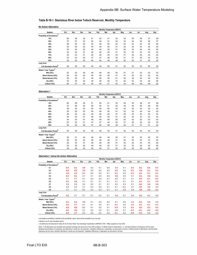
Oct Nov Dec Jan Feb Mar Apr May Jun Jul Aug Sep
10% 60 59 55 51 50 51 53 54 55 56 57 5920% 57 57 53 50 49 51 52 53 54 55 56 5730% 56 55 53 50 49 50 52 53 53 54 55 5640% 55 55 52 49 48 50 51 52 53 54 55 5550% 55 54 52 49 48 50 51 52 53 54 54 5560% 54 54 51 48 48 49 51 52 52 53 54 5470% 54 53 51 48 48 49 50 51 52 52 53 5480% 53 53 50 47 47 48 50 51 51 52 53 5390% 52 52 50 46 46 48 49 50 50 51 52 52
Full Simulation Periodb 56 55 52 49 48 50 51 52 53 54 55 55
Wet (32%) 52 52 49 48 48 49 50 51 51 52 52 53Above Normal (16%) 56 55 52 49 48 49 51 51 52 53 53 54Below Normal (13%) 55 54 51 49 48 50 51 52 52 54 54 55
Dry (24%) 55 55 52 49 48 50 51 52 53 54 55 56Critical (15%) 60 57 54 50 49 51 52 54 56 58 59 62
Oct Nov Dec Jan Feb Mar Apr May Jun Jul Aug Sep
10% 60 59 55 51 50 51 53 54 55 56 57 5820% 57 56 53 50 50 51 52 53 54 55 56 5630% 56 55 53 50 49 50 52 53 53 54 55 5540% 55 55 52 49 49 50 51 52 53 54 54 5550% 55 54 52 49 48 50 51 52 53 53 54 5460% 54 54 51 48 48 49 51 52 52 53 53 5470% 54 53 51 48 48 49 50 52 52 52 53 5380% 53 53 51 47 47 49 50 51 52 52 53 5390% 52 52 50 47 46 48 49 50 51 51 51 52
Full Simulation Periodb 55 55 52 49 48 50 51 52 53 54 55 55
Wet (32%) 52 51 49 48 48 49 50 51 52 52 52 53Above Normal (16%) 56 55 52 49 48 49 51 52 52 53 53 54Below Normal (13%) 55 54 51 49 48 50 51 52 52 53 54 55
Dry (24%) 55 55 52 49 49 50 51 53 53 54 55 56Critical (15%) 59 58 54 50 49 51 52 54 55 58 59 60
Oct Nov Dec Jan Feb Mar Apr May Jun Jul Aug Sep
0.1 -0.7 -0.1 0.0 0.2 0.1 0.2 0.0 0.1 -0.1 -0.1 -0.2 -0.7
0.2 -0.8 -0.3 0.0 0.0 0.2 0.2 -0.2 0.2 -0.1 0.0 -0.1 -0.4
0.3 0.0 0.0 -0.1 0.0 0.2 0.1 -0.1 0.2 -0.1 -0.2 -0.1 -0.1
0.4 -0.1 -0.1 0.1 0.1 0.2 0.0 0.0 0.0 0.1 -0.1 0.0 -0.1
0.5 0.1 0.1 0.1 0.2 0.2 0.1 0.0 0.1 0.1 -0.2 -0.1 -0.2
0.6 -0.1 0.0 0.1 0.1 0.1 0.1 0.1 0.1 0.1 -0.1 -0.1 0.0
0.7 0.0 0.0 0.2 0.2 0.1 0.1 0.2 0.2 0.1 -0.2 0.0 0.0
0.8 0.2 0.2 0.1 0.3 0.5 0.1 0.1 -0.1 0.1 -0.2 0.0 0.00.9 0.1 0.1 -0.1 0.3 0.3 0.1 0.1 0.0 0.5 0.0 0.0 -0.1
Full Simulation Periodb
-0.2 0.1 0.1 0.1 0.2 0.1 0.0 0.1 0.0 -0.2 -0.1 -0.3
Wet (32%) -0.1 -0.1 0.0 0.1 0.2 0.0 0.1 0.0 0.4 -0.2 0.0 0.0Above Normal (16%) -0.2 0.1 0.1 0.1 0.2 0.1 -0.1 0.2 0.0 -0.1 -0.1 -0.1
Below Normal (13%) -0.2 -0.2 -0.1 0.1 0.2 0.1 -0.3 0.3 -0.1 -0.2 -0.2 -0.2
Dry (24%) -0.2 0.0 0.1 0.2 0.2 0.1 0.0 0.1 -0.1 -0.1 -0.2 -0.3
Critical (15%) -0.6 0.7 0.3 0.2 0.2 0.2 -0.1 0.2 -0.9 -0.2 0.2 -1.4
a Exceedance probability is defined as the probability a given value will be exceeded in any one year.
b Based on an 81-year simulation period.
Probability of Exceedancea
Long Term
Water Year Typesc
c As defined by the Sacramento Valley 40-30-30 Index Water Year Hydrologic Classification (SWRCB D-1641, 1999); projected to Year 2030.
Notes: 1) All alternatives are simulated with projected hydrology and sea level at Year 2030 conditions. 2) Model results for Alternatives 1, 4, and Second Basis of Comparison are the same,
therefore Second Basis of Comparison and Alternative 4 results are not presented. Qualitative differences, if applicable, are discussed in the text. 3) Model results for Alternative 2 and No Action
Alternative are the same, therefore Alternative 2 results are not presented. Qualitative differences, if applicable, are discussed in the text.
Probability of Exceedancea
Long Term
Water Year Typesc
Alternative 1 minus No Action Alternative
Statistic
Monthly Temperature (DEG-F)
Long Term
Water Year Typesc
Alternative 1
Statistic
Monthly Temperature (DEG-F)
Table B-16-1. Stanislaus River below Tulloch Reservoir, Monthly Temperature
No Action Alternative
Statistic
Monthly Temperature (DEG-F)
Probability of Exceedancea
Appendix 6B: Surface Water Temperature Modeling
Final LTO EIS 6B.B-303

Oct Nov Dec Jan Feb Mar Apr May Jun Jul Aug Sep
10% 60 59 55 51 50 51 53 54 55 56 57 5920% 57 57 53 50 49 51 52 53 54 55 56 5730% 56 55 53 50 49 50 52 53 53 54 55 5640% 55 55 52 49 48 50 51 52 53 54 55 5550% 55 54 52 49 48 50 51 52 53 54 54 5560% 54 54 51 48 48 49 51 52 52 53 54 5470% 54 53 51 48 48 49 50 51 52 52 53 5480% 53 53 50 47 47 48 50 51 51 52 53 5390% 52 52 50 46 46 48 49 50 50 51 52 52
Full Simulation Periodb 56 55 52 49 48 50 51 52 53 54 55 55
Wet (32%) 52 52 49 48 48 49 50 51 51 52 52 53Above Normal (16%) 56 55 52 49 48 49 51 51 52 53 53 54Below Normal (13%) 55 54 51 49 48 50 51 52 52 54 54 55
Dry (24%) 55 55 52 49 48 50 51 52 53 54 55 56Critical (15%) 60 57 54 50 49 51 52 54 56 58 59 62
Oct Nov Dec Jan Feb Mar Apr May Jun Jul Aug Sep
10% 58 57 54 51 50 51 53 54 55 56 56 5720% 56 56 53 50 50 51 52 53 54 55 55 5630% 55 55 53 49 49 50 52 52 53 54 55 5540% 55 54 52 49 49 50 51 52 53 54 54 5450% 54 54 52 49 48 50 51 52 52 53 54 5460% 54 53 51 48 48 49 51 52 52 53 53 5470% 53 53 51 48 48 49 50 51 52 53 53 5380% 53 53 51 47 47 49 50 51 51 52 53 5390% 52 52 50 47 46 48 49 50 51 51 52 52
Full Simulation Periodb 55 54 52 49 48 50 51 52 53 54 54 55
Wet (32%) 52 51 49 48 48 49 50 51 51 52 52 53Above Normal (16%) 55 54 52 49 48 49 51 51 52 53 53 54Below Normal (13%) 54 53 51 49 48 50 51 52 52 53 54 54
Dry (24%) 55 54 52 49 48 50 52 52 53 54 55 55Critical (15%) 58 57 54 50 49 51 52 54 55 57 59 59
Oct Nov Dec Jan Feb Mar Apr May Jun Jul Aug Sep
0.1 -2.7 -1.6 -0.5 0.1 0.1 0.1 0.1 -0.1 -0.2 -0.8 -1.0 -1.9
0.2 -1.0 -0.7 0.2 -0.3 0.1 0.2 -0.1 -0.1 -0.3 -0.2 -0.4 -1.0
0.3 -0.5 -0.6 0.0 -0.1 0.2 0.1 -0.2 -0.1 -0.2 -0.3 -0.3 -0.5
0.4 -0.5 -0.5 -0.2 0.0 0.2 0.1 0.1 -0.2 -0.1 -0.2 -0.3 -0.5
0.5 -0.3 -0.3 -0.1 0.0 0.2 0.1 0.1 -0.2 -0.1 -0.4 -0.4 -0.5
0.6 -0.3 -0.5 -0.1 0.2 0.0 0.1 0.2 -0.1 -0.2 0.1 -0.2 -0.3
0.7 -0.2 -0.2 -0.1 0.2 0.1 0.1 0.3 0.1 -0.1 0.2 -0.1 -0.3
0.8 -0.3 0.1 0.1 0.3 0.5 0.2 0.2 -0.1 -0.2 0.3 -0.3 -0.3
0.9 -0.1 0.0 -0.3 0.5 0.4 0.3 0.4 -0.1 0.4 0.5 0.2 -0.1
Full Simulation Periodb
-0.8 -0.3 -0.1 0.1 0.2 0.1 0.1 -0.2 -0.2 -0.1 -0.3 -0.8
Wet (32%) -0.4 -0.3 -0.1 0.1 0.4 0.1 0.2 -0.1 0.1 0.3 0.0 -0.2
Above Normal (16%) -0.8 -0.4 0.0 0.1 0.2 0.1 0.1 0.0 -0.1 0.1 -0.2 -0.4
Below Normal (13%) -1.0 -0.7 -0.3 0.0 0.1 0.1 -0.2 -0.1 0.0 -0.2 -0.4 -0.5
Dry (24%) -0.5 -0.4 -0.1 0.0 -0.1 0.0 0.1 -0.1 -0.2 -0.3 -0.6 -0.9
Critical (15%) -1.9 -0.1 0.1 0.2 0.2 0.3 0.0 -0.8 -1.2 -0.7 -0.6 -2.8
a Exceedance probability is defined as the probability a given value will be exceeded in any one year.
b Based on an 81-year simulation period.
Probability of Exceedancea
Long Term
Water Year Typesc
c As defined by the Sacramento Valley 40-30-30 Index Water Year Hydrologic Classification (SWRCB D-1641, 1999); projected to Year 2030.
Notes: 1) All alternatives are simulated with projected hydrology and sea level at Year 2030 conditions. 2) Model results for Alternatives 1, 4, and Second Basis of Comparison are the same,
therefore Alternative 1 and 4 results are not presented. Qualitative differences, if applicable, are discussed in the text. 3) Model results for Alternative 2 and No Action Alternative are the same,
therefore Alternative 2 results are not presented. Qualitative differences, if applicable, are discussed in the text.
Probability of Exceedancea
Long Term
Water Year Typesc
Alternative 3 minus No Action Alternative
Statistic
Monthly Temperature (DEG-F)
Long Term
Water Year Typesc
Alternative 3
Statistic
Monthly Temperature (DEG-F)
Table B-16-2. Stanislaus River below Tulloch Reservoir, Monthly Temperature
No Action Alternative
Statistic
Monthly Temperature (DEG-F)
Probability of Exceedancea
Appendix 6B: Surface Water Temperature Modeling
Final LTO EIS 6B.B-304

Oct Nov Dec Jan Feb Mar Apr May Jun Jul Aug Sep
10% 60 59 55 51 50 51 53 54 55 56 57 5920% 57 57 53 50 49 51 52 53 54 55 56 5730% 56 55 53 50 49 50 52 53 53 54 55 5640% 55 55 52 49 48 50 51 52 53 54 55 5550% 55 54 52 49 48 50 51 52 53 54 54 5560% 54 54 51 48 48 49 51 52 52 53 54 5470% 54 53 51 48 48 49 50 51 52 52 53 5480% 53 53 50 47 47 48 50 51 51 52 53 5390% 52 52 50 46 46 48 49 50 50 51 52 52
Full Simulation Periodb 56 55 52 49 48 50 51 52 53 54 55 55
Wet (32%) 52 52 49 48 48 49 50 51 51 52 52 53Above Normal (16%) 56 55 52 49 48 49 51 51 52 53 53 54Below Normal (13%) 55 54 51 49 48 50 51 52 52 54 54 55
Dry (24%) 55 55 52 49 48 50 51 52 53 54 55 56Critical (15%) 60 57 54 50 49 51 52 54 56 58 59 62
Oct Nov Dec Jan Feb Mar Apr May Jun Jul Aug Sep
10% 65 60 55 51 50 51 53 54 55 57 61 6320% 58 58 54 50 49 51 52 53 54 55 57 5830% 56 56 53 49 49 50 52 53 53 55 56 5640% 55 55 52 49 48 50 52 52 53 54 55 5550% 55 54 52 49 48 50 51 52 53 54 54 5560% 54 54 51 48 48 49 51 52 52 53 54 5470% 54 53 51 48 47 49 50 51 52 52 53 5480% 53 53 50 47 47 48 50 51 51 52 53 5390% 52 52 50 46 46 47 49 50 50 51 51 52
Full Simulation Periodb 56 55 52 49 48 49 51 52 53 54 55 56
Wet (32%) 53 52 49 48 47 49 50 51 51 52 53 53Above Normal (16%) 56 55 52 49 48 49 51 52 52 53 54 54Below Normal (13%) 56 54 52 49 48 49 51 52 53 54 55 56
Dry (24%) 56 55 52 49 48 50 51 53 54 55 56 58Critical (15%) 60 58 54 50 49 50 53 55 55 58 60 62
Oct Nov Dec Jan Feb Mar Apr May Jun Jul Aug Sep
0.1 4.0 1.2 0.4 0.3 -0.2 -0.1 0.3 0.3 0.6 0.6 3.4 4.00.2 1.1 1.4 0.3 -0.1 0.0 0.0 0.1 0.3 0.2 0.4 1.2 1.20.3 0.8 0.6 -0.1 -0.1 -0.1 -0.2 0.1 0.1 0.0 0.5 0.5 0.50.4 0.2 0.2 0.1 -0.1 -0.1 -0.1 0.3 0.1 0.1 0.1 0.3 0.20.5 0.2 0.2 0.2 0.0 0.0 0.0 0.0 0.1 0.0 0.0 0.1 0.00.6 0.3 0.0 0.1 0.1 -0.1 -0.2 0.0 0.2 0.0 0.1 0.0 0.00.7 0.1 0.1 -0.1 0.1 -0.3 -0.1 0.0 0.1 -0.1 0.0 0.0 0.10.8 0.1 0.1 -0.1 0.0 0.0 -0.2 -0.1 -0.3 -0.1 0.0 0.0 0.10.9 0.1 0.0 -0.1 -0.3 -0.2 -0.1 -0.1 -0.1 -0.2 0.0 -0.1 0.2
Full Simulation Periodb 0.6 0.4 0.1 0.0 -0.1 -0.1 0.0 0.2 -0.2 0.1 0.5 0.7
Wet (32%) 0.7 0.3 0.1 0.0 -0.1 -0.1 -0.1 -0.1 -0.1 -0.1 0.0 0.2Above Normal (16%) 0.4 0.4 0.2 0.1 0.0 -0.1 -0.1 0.2 -0.1 0.1 0.2 0.3Below Normal (13%) 0.7 0.0 0.1 -0.1 -0.1 -0.1 0.0 0.2 0.2 0.4 0.6 0.8
Dry (24%) 0.7 0.5 0.2 0.1 0.0 -0.1 0.0 0.1 0.2 0.5 1.1 1.7Critical (15%) 0.5 0.7 -0.2 -0.3 -0.3 -0.2 0.6 0.8 -1.1 -0.2 0.8 0.3
a Exceedance probability is defined as the probability a given value will be exceeded in any one year.
b Based on an 81-year simulation period.
Probability of Exceedancea
Long Term
Water Year Typesc
c As defined by the Sacramento Valley 40-30-30 Index Water Year Hydrologic Classification (SWRCB D-1641, 1999); projected to Year 2030.
Notes: 1) All alternatives are simulated with projected hydrology and sea level at Year 2030 conditions. 2) Model results for Alternatives 1, 4, and Second Basis of Comparison are the same,
therefore Alternative 1 and 4 results are not presented. Qualitative differences, if applicable, are discussed in the text. 3) Model results for Alternative 2 and No Action Alternative are the same,
therefore Alternative 2 results are not presented. Qualitative differences, if applicable, are discussed in the text.
Probability of Exceedancea
Long Term
Water Year Typesc
Alternative 5 minus No Action Alternative
Statistic
Monthly Temperature (DEG-F)
Long Term
Water Year Typesc
Alternative 5
Statistic
Monthly Temperature (DEG-F)
Table B-16-3. Stanislaus River below Tulloch Reservoir, Monthly Temperature
No Action Alternative
Statistic
Monthly Temperature (DEG-F)
Probability of Exceedancea
Appendix 6B: Surface Water Temperature Modeling
Final LTO EIS 6B.B-305

Oct Nov Dec Jan Feb Mar Apr May Jun Jul Aug Sep
10% 60 59 55 51 50 51 53 54 55 56 57 5820% 57 56 53 50 50 51 52 53 54 55 56 5630% 56 55 53 50 49 50 52 53 53 54 55 5540% 55 55 52 49 49 50 51 52 53 54 54 5550% 55 54 52 49 48 50 51 52 53 53 54 5460% 54 54 51 48 48 49 51 52 52 53 53 5470% 54 53 51 48 48 49 50 52 52 52 53 5380% 53 53 51 47 47 49 50 51 52 52 53 5390% 52 52 50 47 46 48 49 50 51 51 51 52
Full Simulation Periodb 55 55 52 49 48 50 51 52 53 54 55 55
Wet (32%) 52 51 49 48 48 49 50 51 52 52 52 53Above Normal (16%) 56 55 52 49 48 49 51 52 52 53 53 54Below Normal (13%) 55 54 51 49 48 50 51 52 52 53 54 55
Dry (24%) 55 55 52 49 49 50 51 53 53 54 55 56Critical (15%) 59 58 54 50 49 51 52 54 55 58 59 60
Oct Nov Dec Jan Feb Mar Apr May Jun Jul Aug Sep
10% 60 59 55 51 50 51 53 54 55 56 57 5920% 57 57 53 50 49 51 52 53 54 55 56 5730% 56 55 53 50 49 50 52 53 53 54 55 5640% 55 55 52 49 48 50 51 52 53 54 55 5550% 55 54 52 49 48 50 51 52 53 54 54 5560% 54 54 51 48 48 49 51 52 52 53 54 5470% 54 53 51 48 48 49 50 51 52 52 53 5480% 53 53 50 47 47 48 50 51 51 52 53 5390% 52 52 50 46 46 48 49 50 50 51 52 52
Full Simulation Periodb 56 55 52 49 48 50 51 52 53 54 55 55
Wet (32%) 52 52 49 48 48 49 50 51 51 52 52 53Above Normal (16%) 56 55 52 49 48 49 51 51 52 53 53 54Below Normal (13%) 55 54 51 49 48 50 51 52 52 54 54 55
Dry (24%) 55 55 52 49 48 50 51 52 53 54 55 56Critical (15%) 60 57 54 50 49 51 52 54 56 58 59 62
Oct Nov Dec Jan Feb Mar Apr May Jun Jul Aug Sep
0.1 0.7 0.1 0.0 -0.2 -0.1 -0.2 0.0 -0.1 0.1 0.1 0.2 0.70.2 0.8 0.3 0.0 0.0 -0.2 -0.2 0.2 -0.2 0.1 0.0 0.1 0.40.3 0.0 0.0 0.1 0.0 -0.2 -0.1 0.1 -0.2 0.1 0.2 0.1 0.10.4 0.1 0.1 -0.1 -0.1 -0.2 0.0 0.0 0.0 -0.1 0.1 0.0 0.10.5 -0.1 -0.1 -0.1 -0.2 -0.2 -0.1 0.0 -0.1 -0.1 0.2 0.1 0.20.6 0.1 0.0 -0.1 -0.1 -0.1 -0.1 -0.1 -0.1 -0.1 0.1 0.1 0.00.7 0.0 0.0 -0.2 -0.2 -0.1 -0.1 -0.2 -0.2 -0.1 0.2 0.0 0.00.8 -0.2 -0.2 -0.1 -0.3 -0.5 -0.1 -0.1 0.1 -0.1 0.2 0.0 0.0
0.9 -0.1 -0.1 0.1 -0.3 -0.3 -0.1 -0.1 0.0 -0.5 0.0 0.0 0.1
Full Simulation Periodb 0.2 -0.1 -0.1 -0.1 -0.2 -0.1 0.0 -0.1 0.0 0.2 0.1 0.3
Wet (32%) 0.1 0.1 0.0 -0.1 -0.2 0.0 -0.1 0.0 -0.4 0.2 0.0 0.0
Above Normal (16%) 0.2 -0.1 -0.1 -0.1 -0.2 -0.1 0.1 -0.2 0.0 0.1 0.1 0.1Below Normal (13%) 0.2 0.2 0.1 -0.1 -0.2 -0.1 0.3 -0.3 0.1 0.2 0.2 0.2
Dry (24%) 0.2 0.0 -0.1 -0.2 -0.2 -0.1 0.0 -0.1 0.1 0.1 0.2 0.3Critical (15%) 0.6 -0.7 -0.3 -0.2 -0.2 -0.2 0.1 -0.2 0.9 0.2 -0.2 1.4
a Exceedance probability is defined as the probability a given value will be exceeded in any one year.
b Based on an 81-year simulation period.
Probability of Exceedancea
Long Term
Water Year Typesc
c As defined by the Sacramento Valley 40-30-30 Index Water Year Hydrologic Classification (SWRCB D-1641, 1999); projected to Year 2030.
Notes: 1) All alternatives are simulated with projected hydrology and sea level at Year 2030 conditions. 2) Model results for Alternatives 1, 4, and Second Basis of Comparison are the same,
therefore Alternative 1 and 4 results are not presented. Qualitative differences, if applicable, are discussed in the text. 3) Model results for Alternative 2 and No Action Alternative are the same,
therefore Alternative 2 results are not presented. Qualitative differences, if applicable, are discussed in the text.
Probability of Exceedancea
Long Term
Water Year Typesc
No Action Alternative minus Second Basis of Comparison
Statistic
Monthly Temperature (DEG-F)
Long Term
Water Year Typesc
No Action Alternative
Statistic
Monthly Temperature (DEG-F)
Table B-16-4. Stanislaus River below Tulloch Reservoir, Monthly Temperature
Second Basis of Comparison
Statistic
Monthly Temperature (DEG-F)
Probability of Exceedancea
Appendix 6B: Surface Water Temperature Modeling
Final LTO EIS 6B.B-306

Oct Nov Dec Jan Feb Mar Apr May Jun Jul Aug Sep
10% 60 59 55 51 50 51 53 54 55 56 57 5820% 57 56 53 50 50 51 52 53 54 55 56 5630% 56 55 53 50 49 50 52 53 53 54 55 5540% 55 55 52 49 49 50 51 52 53 54 54 5550% 55 54 52 49 48 50 51 52 53 53 54 5460% 54 54 51 48 48 49 51 52 52 53 53 5470% 54 53 51 48 48 49 50 52 52 52 53 5380% 53 53 51 47 47 49 50 51 52 52 53 5390% 52 52 50 47 46 48 49 50 51 51 51 52
Full Simulation Periodb 55 55 52 49 48 50 51 52 53 54 55 55
Wet (32%) 52 51 49 48 48 49 50 51 52 52 52 53Above Normal (16%) 56 55 52 49 48 49 51 52 52 53 53 54Below Normal (13%) 55 54 51 49 48 50 51 52 52 53 54 55
Dry (24%) 55 55 52 49 49 50 51 53 53 54 55 56Critical (15%) 59 58 54 50 49 51 52 54 55 58 59 60
Oct Nov Dec Jan Feb Mar Apr May Jun Jul Aug Sep
10% 58 57 54 51 50 51 53 54 55 56 56 5720% 56 56 53 50 50 51 52 53 54 55 55 5630% 55 55 53 49 49 50 52 52 53 54 55 5540% 55 54 52 49 49 50 51 52 53 54 54 5450% 54 54 52 49 48 50 51 52 52 53 54 5460% 54 53 51 48 48 49 51 52 52 53 53 5470% 53 53 51 48 48 49 50 51 52 53 53 5380% 53 53 51 47 47 49 50 51 51 52 53 5390% 52 52 50 47 46 48 49 50 51 51 52 52
Full Simulation Periodb 55 54 52 49 48 50 51 52 53 54 54 55
Wet (32%) 52 51 49 48 48 49 50 51 51 52 52 53Above Normal (16%) 55 54 52 49 48 49 51 51 52 53 53 54Below Normal (13%) 54 53 51 49 48 50 51 52 52 53 54 54
Dry (24%) 55 54 52 49 48 50 52 52 53 54 55 55Critical (15%) 58 57 54 50 49 51 52 54 55 57 59 59
Oct Nov Dec Jan Feb Mar Apr May Jun Jul Aug Sep
0.1 -2.0 -1.5 -0.4 -0.1 -0.1 -0.1 0.1 -0.2 -0.1 -0.7 -0.8 -1.2
0.2 -0.2 -0.4 0.2 -0.3 -0.1 0.0 0.1 -0.3 -0.2 -0.2 -0.3 -0.6
0.3 -0.5 -0.6 0.1 -0.1 0.1 0.0 -0.1 -0.4 -0.1 -0.1 -0.2 -0.4
0.4 -0.4 -0.4 -0.3 -0.2 0.0 0.0 0.1 -0.2 -0.2 -0.2 -0.3 -0.4
0.5 -0.4 -0.4 -0.2 -0.2 0.0 0.0 0.0 -0.3 -0.2 -0.2 -0.3 -0.3
0.6 -0.2 -0.5 -0.2 0.1 -0.1 0.0 0.1 -0.2 -0.3 0.2 -0.1 -0.3
0.7 -0.2 -0.2 -0.3 0.0 0.0 0.0 0.2 -0.1 -0.2 0.4 -0.1 -0.3
0.8 -0.4 -0.1 0.0 0.0 0.1 0.0 0.2 0.0 -0.3 0.5 -0.2 -0.3
0.9 -0.1 -0.1 -0.2 0.2 0.1 0.2 0.3 -0.1 -0.1 0.6 0.3 0.0
Full Simulation Periodb
-0.5 -0.4 -0.1 -0.1 0.0 0.0 0.1 -0.3 -0.2 0.1 -0.3 -0.5
Wet (32%) -0.3 -0.2 -0.1 0.0 0.3 0.0 0.1 -0.2 -0.3 0.5 0.0 -0.2
Above Normal (16%) -0.5 -0.4 -0.2 0.0 0.0 0.0 0.2 -0.2 -0.1 0.1 -0.1 -0.3
Below Normal (13%) -0.7 -0.5 -0.2 -0.1 -0.1 -0.1 0.1 -0.3 0.0 -0.1 -0.2 -0.3
Dry (24%) -0.3 -0.3 -0.1 -0.1 -0.3 -0.1 0.1 -0.2 -0.1 -0.2 -0.5 -0.7
Critical (15%) -1.3 -0.8 -0.2 -0.1 -0.1 0.1 0.1 -0.9 -0.2 -0.5 -0.8 -1.5
a Exceedance probability is defined as the probability a given value will be exceeded in any one year.
b Based on an 81-year simulation period.
Probability of Exceedancea
Long Term
Water Year Typesc
c As defined by the Sacramento Valley 40-30-30 Index Water Year Hydrologic Classification (SWRCB D-1641, 1999); projected to Year 2030.
Notes: 1) All alternatives are simulated with projected hydrology and sea level at Year 2030 conditions. 2) Model results for Alternatives 1, 4, and Second Basis of Comparison are the same,
therefore Alternative 1 and 4 results are not presented. Qualitative differences, if applicable, are discussed in the text. 3) Model results for Alternative 2 and No Action Alternative are the same,
therefore Alternative 2 results are not presented. Qualitative differences, if applicable, are discussed in the text.
Probability of Exceedancea
Long Term
Water Year Typesc
Alternative 3 minus Second Basis of Comparison
Statistic
Monthly Temperature (DEG-F)
Long Term
Water Year Typesc
Alternative 3
Statistic
Monthly Temperature (DEG-F)
Table B-16-5. Stanislaus River below Tulloch Reservoir, Monthly Temperature
Second Basis of Comparison
Statistic
Monthly Temperature (DEG-F)
Probability of Exceedancea
Appendix 6B: Surface Water Temperature Modeling
Final LTO EIS 6B.B-307

Oct Nov Dec Jan Feb Mar Apr May Jun Jul Aug Sep
10% 60 59 55 51 50 51 53 54 55 56 57 5820% 57 56 53 50 50 51 52 53 54 55 56 5630% 56 55 53 50 49 50 52 53 53 54 55 5540% 55 55 52 49 49 50 51 52 53 54 54 5550% 55 54 52 49 48 50 51 52 53 53 54 5460% 54 54 51 48 48 49 51 52 52 53 53 5470% 54 53 51 48 48 49 50 52 52 52 53 5380% 53 53 51 47 47 49 50 51 52 52 53 5390% 52 52 50 47 46 48 49 50 51 51 51 52
Full Simulation Periodb 55 55 52 49 48 50 51 52 53 54 55 55
Wet (32%) 52 51 49 48 48 49 50 51 52 52 52 53Above Normal (16%) 56 55 52 49 48 49 51 52 52 53 53 54Below Normal (13%) 55 54 51 49 48 50 51 52 52 53 54 55
Dry (24%) 55 55 52 49 49 50 51 53 53 54 55 56Critical (15%) 59 58 54 50 49 51 52 54 55 58 59 60
Oct Nov Dec Jan Feb Mar Apr May Jun Jul Aug Sep
10% 65 60 55 51 50 51 53 54 55 57 61 6320% 58 58 54 50 49 51 52 53 54 55 57 5830% 56 56 53 49 49 50 52 53 53 55 56 5640% 55 55 52 49 48 50 52 52 53 54 55 5550% 55 54 52 49 48 50 51 52 53 54 54 5560% 54 54 51 48 48 49 51 52 52 53 54 5470% 54 53 51 48 47 49 50 51 52 52 53 5480% 53 53 50 47 47 48 50 51 51 52 53 5390% 52 52 50 46 46 47 49 50 50 51 51 52
Full Simulation Periodb 56 55 52 49 48 49 51 52 53 54 55 56
Wet (32%) 53 52 49 48 47 49 50 51 51 52 53 53Above Normal (16%) 56 55 52 49 48 49 51 52 52 53 54 54Below Normal (13%) 56 54 52 49 48 49 51 52 53 54 55 56
Dry (24%) 56 55 52 49 48 50 51 53 54 55 56 58Critical (15%) 60 58 54 50 49 50 53 55 55 58 60 62
Oct Nov Dec Jan Feb Mar Apr May Jun Jul Aug Sep
0.1 4.8 1.3 0.4 0.1 -0.3 -0.3 0.2 0.2 0.7 0.7 3.5 4.80.2 1.8 1.7 0.3 -0.1 -0.2 -0.2 0.3 0.1 0.2 0.4 1.3 1.60.3 0.8 0.6 0.0 -0.2 -0.3 -0.2 0.2 -0.2 0.1 0.6 0.6 0.60.4 0.3 0.3 0.0 -0.2 -0.3 -0.1 0.3 0.0 -0.1 0.2 0.4 0.30.5 0.1 0.1 0.1 -0.2 -0.2 -0.2 0.0 0.0 -0.1 0.2 0.2 0.20.6 0.4 0.0 0.0 0.0 -0.2 -0.3 0.0 0.0 -0.2 0.2 0.1 0.10.7 0.1 0.1 -0.2 -0.1 -0.4 -0.2 -0.1 -0.1 -0.2 0.2 0.1 0.20.8 -0.1 -0.1 -0.1 -0.3 -0.5 -0.4 -0.1 -0.2 -0.2 0.2 0.1 0.00.9 0.0 -0.1 0.0 -0.7 -0.6 -0.2 -0.2 -0.1 -0.6 0.0 0.0 0.3
Full Simulation Periodb 0.9 0.3 0.0 -0.1 -0.3 -0.2 0.1 0.0 -0.1 0.3 0.6 1.0
Wet (32%) 0.9 0.4 0.1 -0.1 -0.2 -0.1 -0.2 -0.1 -0.5 0.2 0.1 0.1Above Normal (16%) 0.7 0.4 0.1 -0.1 -0.2 -0.2 0.0 0.0 -0.1 0.2 0.3 0.4Below Normal (13%) 0.9 0.2 0.1 -0.2 -0.3 -0.2 0.2 -0.1 0.3 0.6 0.8 1.0
Dry (24%) 0.8 0.5 0.2 -0.1 -0.2 -0.2 0.0 0.0 0.2 0.6 1.3 1.9Critical (15%) 1.1 0.0 -0.5 -0.5 -0.6 -0.4 0.7 0.7 -0.2 0.0 0.6 1.7
a Exceedance probability is defined as the probability a given value will be exceeded in any one year.
b Based on an 81-year simulation period.
Probability of Exceedancea
Long Term
Water Year Typesc
c As defined by the Sacramento Valley 40-30-30 Index Water Year Hydrologic Classification (SWRCB D-1641, 1999); projected to Year 2030.
Notes: 1) All alternatives are simulated with projected hydrology and sea level at Year 2030 conditions. 2) Model results for Alternatives 1, 4, and Second Basis of Comparison are the same,
therefore Alternative 1 and 4 results are not presented. Qualitative differences, if applicable, are discussed in the text. 3) Model results for Alternative 2 and No Action Alternative are the same,
therefore Alternative 2 results are not presented. Qualitative differences, if applicable, are discussed in the text.
Probability of Exceedancea
Long Term
Water Year Typesc
Alternative 5 minus Second Basis of Comparison
Statistic
Monthly Temperature (DEG-F)
Long Term
Water Year Typesc
Alternative 5
Statistic
Monthly Temperature (DEG-F)
Table B-16-6. Stanislaus River below Tulloch Reservoir, Monthly Temperature
Second Basis of Comparison
Statistic
Monthly Temperature (DEG-F)
Probability of Exceedancea
Appendix 6B: Surface Water Temperature Modeling
Final LTO EIS 6B.B-308

B.17. Stanislaus River below Goodwin Temperature
Appendix 6B: Surface Water Temperature Modeling
Final LTO EIS 6B.B-309
1

Figure B-17-1. Stanislaus River below Goodwin Dam, October
Notes: 1) Exceedance probability is defined as the probability a given value will be exceeded in any one year. 2) All alternatives are simulated with projected hydrology and
sea level at Year 2030 conditions. 3) Model results for Alternatives 1, 4, and Second Basis of Comparison are the same, therefore Alternatives 1 and 4 results are not
presented. Qualitative differences, if applicable, are discussed in the text. 4) Model results for Alternative 2 and No Action Alternative are the same, therefore Alternative 2
results are not presented. Qualitative differences, if applicable, are discussed in the text.
44
46
48
50
52
54
56
58
60
62
64
66
68
70
72
0%10%20%30%40%50%60%70%80%90%100%
Exceedance Probability
No Action Alternative & Alternative 2 Second Basis of Comparison, Alternative 1, & Alternative 4
Alternative 3 Alternative 5
Mon
thly
Tem
pera
ture
(DE
G-F
)
Appendix 6B: Surface Water Temperature Modeling
Final LTO EIS 6B.B-310

Figure B-17-2. Stanislaus River below Goodwin Dam, November
Notes: 1) Exceedance probability is defined as the probability a given value will be exceeded in any one year. 2) All alternatives are simulated with projected hydrology and
sea level at Year 2030 conditions. 3) Model results for Alternatives 1, 4, and Second Basis of Comparison are the same, therefore Alternatives 1 and 4 results are not
presented. Qualitative differences, if applicable, are discussed in the text. 4) Model results for Alternative 2 and No Action Alternative are the same, therefore Alternative 2
results are not presented. Qualitative differences, if applicable, are discussed in the text.
44
46
48
50
52
54
56
58
60
62
64
66
68
70
72
0%10%20%30%40%50%60%70%80%90%100%
Exceedance Probability
No Action Alternative & Alternative 2 Second Basis of Comparison, Alternative 1, & Alternative 4
Alternative 3 Alternative 5
Mon
thly
Tem
pera
ture
(DE
G-F
)
Appendix 6B: Surface Water Temperature Modeling
Final LTO EIS 6B.B-311

Figure B-17-3. Stanislaus River below Goodwin Dam, December
Notes: 1) Exceedance probability is defined as the probability a given value will be exceeded in any one year. 2) All alternatives are simulated with projected hydrology and
sea level at Year 2030 conditions. 3) Model results for Alternatives 1, 4, and Second Basis of Comparison are the same, therefore Alternatives 1 and 4 results are not
presented. Qualitative differences, if applicable, are discussed in the text. 4) Model results for Alternative 2 and No Action Alternative are the same, therefore Alternative 2
results are not presented. Qualitative differences, if applicable, are discussed in the text.
44
46
48
50
52
54
56
58
60
62
64
66
68
70
72
0%10%20%30%40%50%60%70%80%90%100%
Exceedance Probability
No Action Alternative & Alternative 2 Second Basis of Comparison, Alternative 1, & Alternative 4
Alternative 3 Alternative 5
Mon
thly
Tem
pera
ture
(DE
G-F
)
Appendix 6B: Surface Water Temperature Modeling
Final LTO EIS 6B.B-312

Figure B-17-4. Stanislaus River below Goodwin Dam, January
Notes: 1) Exceedance probability is defined as the probability a given value will be exceeded in any one year. 2) All alternatives are simulated with projected hydrology and
sea level at Year 2030 conditions. 3) Model results for Alternatives 1, 4, and Second Basis of Comparison are the same, therefore Alternatives 1 and 4 results are not
presented. Qualitative differences, if applicable, are discussed in the text. 4) Model results for Alternative 2 and No Action Alternative are the same, therefore Alternative 2
results are not presented. Qualitative differences, if applicable, are discussed in the text.
44
46
48
50
52
54
56
58
60
62
64
66
68
70
72
0%10%20%30%40%50%60%70%80%90%100%
Exceedance Probability
No Action Alternative & Alternative 2 Second Basis of Comparison, Alternative 1, & Alternative 4
Alternative 3 Alternative 5
Mon
thly
Tem
pera
ture
(DE
G-F
)
Appendix 6B: Surface Water Temperature Modeling
Final LTO EIS 6B.B-313

Figure B-17-5. Stanislaus River below Goodwin Dam, February
Notes: 1) Exceedance probability is defined as the probability a given value will be exceeded in any one year. 2) All alternatives are simulated with projected hydrology and
sea level at Year 2030 conditions. 3) Model results for Alternatives 1, 4, and Second Basis of Comparison are the same, therefore Alternatives 1 and 4 results are not
presented. Qualitative differences, if applicable, are discussed in the text. 4) Model results for Alternative 2 and No Action Alternative are the same, therefore Alternative 2
results are not presented. Qualitative differences, if applicable, are discussed in the text.
44
46
48
50
52
54
56
58
60
62
64
66
68
70
72
0%10%20%30%40%50%60%70%80%90%100%
Exceedance Probability
No Action Alternative & Alternative 2 Second Basis of Comparison, Alternative 1, & Alternative 4
Alternative 3 Alternative 5
Mon
thly
Tem
pera
ture
(DE
G-F
)
Appendix 6B: Surface Water Temperature Modeling
Final LTO EIS 6B.B-314

Figure B-17-6. Stanislaus River below Goodwin Dam, March
Notes: 1) Exceedance probability is defined as the probability a given value will be exceeded in any one year. 2) All alternatives are simulated with projected hydrology and
sea level at Year 2030 conditions. 3) Model results for Alternatives 1, 4, and Second Basis of Comparison are the same, therefore Alternatives 1 and 4 results are not
presented. Qualitative differences, if applicable, are discussed in the text. 4) Model results for Alternative 2 and No Action Alternative are the same, therefore Alternative 2
results are not presented. Qualitative differences, if applicable, are discussed in the text.
44
46
48
50
52
54
56
58
60
62
64
66
68
70
72
0%10%20%30%40%50%60%70%80%90%100%
Exceedance Probability
No Action Alternative & Alternative 2 Second Basis of Comparison, Alternative 1, & Alternative 4
Alternative 3 Alternative 5
Mon
thly
Tem
pera
ture
(DE
G-F
)
Appendix 6B: Surface Water Temperature Modeling
Final LTO EIS 6B.B-315

Figure B-17-7. Stanislaus River below Goodwin Dam, April
Notes: 1) Exceedance probability is defined as the probability a given value will be exceeded in any one year. 2) All alternatives are simulated with projected hydrology and
sea level at Year 2030 conditions. 3) Model results for Alternatives 1, 4, and Second Basis of Comparison are the same, therefore Alternatives 1 and 4 results are not
presented. Qualitative differences, if applicable, are discussed in the text. 4) Model results for Alternative 2 and No Action Alternative are the same, therefore Alternative 2
results are not presented. Qualitative differences, if applicable, are discussed in the text.
44
46
48
50
52
54
56
58
60
62
64
66
68
70
72
0%10%20%30%40%50%60%70%80%90%100%
Exceedance Probability
No Action Alternative & Alternative 2 Second Basis of Comparison, Alternative 1, & Alternative 4
Alternative 3 Alternative 5
Mon
thly
Tem
pera
ture
(DE
G-F
)
Appendix 6B: Surface Water Temperature Modeling
Final LTO EIS 6B.B-316

Figure B-17-8. Stanislaus River below Goodwin Dam, May
Notes: 1) Exceedance probability is defined as the probability a given value will be exceeded in any one year. 2) All alternatives are simulated with projected hydrology and
sea level at Year 2030 conditions. 3) Model results for Alternatives 1, 4, and Second Basis of Comparison are the same, therefore Alternatives 1 and 4 results are not
presented. Qualitative differences, if applicable, are discussed in the text. 4) Model results for Alternative 2 and No Action Alternative are the same, therefore Alternative 2
results are not presented. Qualitative differences, if applicable, are discussed in the text.
44
46
48
50
52
54
56
58
60
62
64
66
68
70
72
0%10%20%30%40%50%60%70%80%90%100%
Exceedance Probability
No Action Alternative & Alternative 2 Second Basis of Comparison, Alternative 1, & Alternative 4
Alternative 3 Alternative 5
Mon
thly
Tem
pera
ture
(DE
G-F
)
Appendix 6B: Surface Water Temperature Modeling
Final LTO EIS 6B.B-317

Figure B-17-9. Stanislaus River below Goodwin Dam, June
Notes: 1) Exceedance probability is defined as the probability a given value will be exceeded in any one year. 2) All alternatives are simulated with projected hydrology and
sea level at Year 2030 conditions. 3) Model results for Alternatives 1, 4, and Second Basis of Comparison are the same, therefore Alternatives 1 and 4 results are not
presented. Qualitative differences, if applicable, are discussed in the text. 4) Model results for Alternative 2 and No Action Alternative are the same, therefore Alternative 2
results are not presented. Qualitative differences, if applicable, are discussed in the text.
44
46
48
50
52
54
56
58
60
62
64
66
68
70
72
0%10%20%30%40%50%60%70%80%90%100%
Exceedance Probability
No Action Alternative & Alternative 2 Second Basis of Comparison, Alternative 1, & Alternative 4
Alternative 3 Alternative 5
Mon
thly
Tem
pera
ture
(DE
G-F
)
Appendix 6B: Surface Water Temperature Modeling
Final LTO EIS 6B.B-318

Figure B-17-10. Stanislaus River below Goodwin Dam, July
Notes: 1) Exceedance probability is defined as the probability a given value will be exceeded in any one year. 2) All alternatives are simulated with projected hydrology and
sea level at Year 2030 conditions. 3) Model results for Alternatives 1, 4, and Second Basis of Comparison are the same, therefore Alternatives 1 and 4 results are not
presented. Qualitative differences, if applicable, are discussed in the text. 4) Model results for Alternative 2 and No Action Alternative are the same, therefore Alternative 2
results are not presented. Qualitative differences, if applicable, are discussed in the text.
44
46
48
50
52
54
56
58
60
62
64
66
68
70
72
0%10%20%30%40%50%60%70%80%90%100%
Exceedance Probability
No Action Alternative & Alternative 2 Second Basis of Comparison, Alternative 1, & Alternative 4
Alternative 3 Alternative 5
Mon
thly
Tem
pera
ture
(DE
G-F
)
Appendix 6B: Surface Water Temperature Modeling
Final LTO EIS 6B.B-319

Figure B-17-11. Stanislaus River below Goodwin Dam, August
Notes: 1) Exceedance probability is defined as the probability a given value will be exceeded in any one year. 2) All alternatives are simulated with projected hydrology and
sea level at Year 2030 conditions. 3) Model results for Alternatives 1, 4, and Second Basis of Comparison are the same, therefore Alternatives 1 and 4 results are not
presented. Qualitative differences, if applicable, are discussed in the text. 4) Model results for Alternative 2 and No Action Alternative are the same, therefore Alternative 2
results are not presented. Qualitative differences, if applicable, are discussed in the text.
44
46
48
50
52
54
56
58
60
62
64
66
68
70
72
0%10%20%30%40%50%60%70%80%90%100%
Exceedance Probability
No Action Alternative & Alternative 2 Second Basis of Comparison, Alternative 1, & Alternative 4
Alternative 3 Alternative 5
Mon
thly
Tem
pera
ture
(DE
G-F
)
Appendix 6B: Surface Water Temperature Modeling
Final LTO EIS 6B.B-320

Figure B-17-12. Stanislaus River below Goodwin Dam, September
Notes: 1) Exceedance probability is defined as the probability a given value will be exceeded in any one year. 2) All alternatives are simulated with projected hydrology and
sea level at Year 2030 conditions. 3) Model results for Alternatives 1, 4, and Second Basis of Comparison are the same, therefore Alternatives 1 and 4 results are not
presented. Qualitative differences, if applicable, are discussed in the text. 4) Model results for Alternative 2 and No Action Alternative are the same, therefore Alternative 2
results are not presented. Qualitative differences, if applicable, are discussed in the text.
44
46
48
50
52
54
56
58
60
62
64
66
68
70
72
0%10%20%30%40%50%60%70%80%90%100%
Exceedance Probability
No Action Alternative & Alternative 2 Second Basis of Comparison, Alternative 1, & Alternative 4
Alternative 3 Alternative 5
Mon
thly
Tem
pera
ture
(DE
G-F
)
Appendix 6B: Surface Water Temperature Modeling
6B.B-321

Oct Nov Dec Jan Feb Mar Apr May Jun Jul Aug Sep
10% 61 59 55 51 51 52 53 54 56 58 58 6020% 58 57 53 50 50 51 52 54 55 56 56 5730% 56 56 53 50 49 51 52 53 54 55 56 5640% 55 55 52 49 49 51 52 53 54 55 55 5650% 55 54 52 49 49 50 51 53 53 54 55 5560% 55 54 51 48 48 50 51 52 53 53 54 5570% 54 54 51 48 48 50 51 52 52 53 54 5480% 54 53 50 47 47 49 50 51 52 53 53 5490% 52 52 50 46 47 48 49 51 51 52 52 53
Full Simulation Periodb 56 55 52 49 49 50 51 53 53 55 55 56
Wet (32%) 52 52 49 48 48 49 50 52 52 53 53 53Above Normal (16%) 56 55 52 49 49 50 51 52 53 53 54 55Below Normal (13%) 55 54 51 49 49 50 52 52 53 54 55 56
Dry (24%) 56 55 52 49 49 51 52 53 54 55 56 57Critical (15%) 60 58 54 50 50 51 53 55 57 59 60 63
Oct Nov Dec Jan Feb Mar Apr May Jun Jul Aug Sep
10% 60 59 55 51 51 52 53 54 56 57 58 5920% 57 56 53 50 50 51 52 54 55 56 56 5730% 56 55 53 50 50 51 52 53 54 55 56 5640% 56 55 52 49 49 51 52 53 54 55 55 5650% 55 54 52 49 49 50 51 53 53 54 55 5560% 55 54 51 49 49 50 51 52 53 53 54 5570% 54 53 51 48 48 50 51 52 52 53 54 5480% 54 53 51 48 48 49 50 51 52 52 53 5490% 53 52 50 47 47 48 49 51 51 51 52 52
Full Simulation Periodb 56 55 52 49 49 50 51 53 53 54 55 56
Wet (32%) 52 52 49 48 48 49 50 52 52 52 53 53Above Normal (16%) 56 55 52 49 49 50 51 52 53 53 54 55Below Normal (13%) 55 54 51 49 49 50 51 53 53 54 55 55
Dry (24%) 56 55 52 49 49 51 52 53 54 55 56 57Critical (15%) 60 58 54 50 50 52 53 55 56 59 60 61
Oct Nov Dec Jan Feb Mar Apr May Jun Jul Aug Sep
0.1 -0.5 -0.1 -0.1 0.0 0.0 0.0 0.0 0.1 -0.1 -0.2 -0.2 -0.9
0.2 -0.7 -0.1 0.0 0.0 0.1 0.0 0.0 0.0 0.0 0.1 -0.1 -0.4
0.3 0.3 -0.1 0.2 0.1 0.1 0.1 -0.1 0.2 -0.1 -0.2 -0.1 -0.2
0.4 0.2 -0.1 0.1 0.0 0.2 0.1 0.0 0.1 0.0 -0.1 0.0 -0.1
0.5 0.3 0.1 0.1 0.1 0.0 0.1 0.0 0.0 0.0 -0.2 -0.1 -0.1
0.6 0.3 0.1 0.2 0.1 0.2 0.1 0.1 0.1 0.3 -0.1 -0.1 0.00.7 0.5 0.0 0.1 0.2 0.1 0.1 0.1 0.1 0.0 -0.1 -0.1 -0.1
0.8 0.3 0.0 0.1 0.3 0.3 0.1 0.1 0.0 0.0 -0.2 0.1 0.00.9 0.3 0.1 0.0 0.4 0.1 0.0 0.1 0.0 0.3 -0.3 0.0 -0.3
Full Simulation Periodb 0.0 0.0 0.1 0.1 0.1 0.1 0.0 0.1 -0.1 -0.2 -0.1 -0.3
Wet (32%) 0.1 -0.1 0.0 0.1 0.1 0.1 0.1 0.1 0.3 -0.2 0.0 0.0Above Normal (16%) 0.1 0.0 0.1 0.1 0.1 0.1 0.0 0.2 0.0 -0.1 -0.1 -0.1
Below Normal (13%) 0.0 -0.2 0.0 0.1 0.1 0.1 -0.2 0.2 -0.1 -0.2 -0.2 -0.2
Dry (24%) 0.1 -0.1 0.1 0.1 0.1 0.1 0.1 0.1 -0.1 -0.1 -0.1 -0.3
Critical (15%) -0.4 0.7 0.4 0.2 0.2 0.2 0.0 0.1 -0.8 -0.3 0.1 -1.3
a Exceedance probability is defined as the probability a given value will be exceeded in any one year.
b Based on an 81-year simulation period.
Probability of Exceedancea
Long Term
Water Year Typesc
c As defined by the Sacramento Valley 40-30-30 Index Water Year Hydrologic Classification (SWRCB D-1641, 1999); projected to Year 2030.
Notes: 1) All alternatives are simulated with projected hydrology and sea level at Year 2030 conditions. 2) Model results for Alternatives 1, 4, and Second Basis of Comparison are the same,
therefore Second Basis of Comparison and Alternative 4 results are not presented. Qualitative differences, if applicable, are discussed in the text. 3) Model results for Alternative 2 and No Action
Alternative are the same, therefore Alternative 2 results are not presented. Qualitative differences, if applicable, are discussed in the text.
Probability of Exceedancea
Long Term
Water Year Typesc
Alternative 1 minus No Action Alternative
Statistic
Monthly Temperature (DEG-F)
Long Term
Water Year Typesc
Alternative 1
Statistic
Monthly Temperature (DEG-F)
No Action Alternative
Statistic
Monthly Temperature (DEG-F)
Probability of Exceedancea
Table B-17-1. Stanislaus River below Goodwin Dam, Monthly Temperature
Appendix 6B: Surface Water Temperature Modeling
6B.B-322

Oct Nov Dec Jan Feb Mar Apr May Jun Jul Aug Sep
10% 61 59 55 51 51 52 53 54 56 58 58 6020% 58 57 53 50 50 51 52 54 55 56 56 5730% 56 56 53 50 49 51 52 53 54 55 56 5640% 55 55 52 49 49 51 52 53 54 55 55 5650% 55 54 52 49 49 50 51 53 53 54 55 5560% 55 54 51 48 48 50 51 52 53 53 54 5570% 54 54 51 48 48 50 51 52 52 53 54 5480% 54 53 50 47 47 49 50 51 52 53 53 5490% 52 52 50 46 47 48 49 51 51 52 52 53
Full Simulation Periodb 56 55 52 49 49 50 51 53 53 55 55 56
Wet (32%) 52 52 49 48 48 49 50 52 52 53 53 53Above Normal (16%) 56 55 52 49 49 50 51 52 53 53 54 55Below Normal (13%) 55 54 51 49 49 50 52 52 53 54 55 56
Dry (24%) 56 55 52 49 49 51 52 53 54 55 56 57Critical (15%) 60 58 54 50 50 51 53 55 57 59 60 63
Oct Nov Dec Jan Feb Mar Apr May Jun Jul Aug Sep
10% 59 58 54 51 51 52 53 54 55 57 57 5820% 57 56 53 50 50 51 52 53 55 56 56 5730% 56 55 53 50 49 51 52 53 54 55 55 5640% 55 54 52 49 49 51 52 53 53 54 55 5550% 55 54 51 49 49 50 51 52 53 54 55 5560% 55 54 51 49 48 50 51 52 53 54 54 5470% 54 53 51 48 48 50 51 52 52 53 54 5480% 53 53 50 48 48 49 50 51 52 53 53 5390% 53 52 50 47 47 49 50 51 51 52 52 52
Full Simulation Periodb 55 55 52 49 49 50 51 52 53 54 55 55
Wet (32%) 52 51 49 48 48 50 50 51 52 53 53 53Above Normal (16%) 56 55 52 49 49 50 51 52 53 54 54 54Below Normal (13%) 55 54 51 49 49 50 51 52 53 54 55 55
Dry (24%) 55 54 52 49 49 51 52 53 54 55 55 56Critical (15%) 59 57 54 50 50 52 53 54 56 58 60 60
Oct Nov Dec Jan Feb Mar Apr May Jun Jul Aug Sep
0.1 -2.2 -1.5 -0.5 -0.1 0.0 0.2 0.0 -0.1 -0.2 -0.8 -1.0 -1.9
0.2 -1.0 -0.6 0.0 -0.3 -0.1 0.0 0.0 -0.1 -0.2 -0.3 -0.5 -0.8
0.3 -0.2 -0.8 0.3 0.0 0.0 0.1 -0.1 -0.2 -0.1 -0.3 -0.4 -0.5
0.4 -0.3 -0.4 -0.2 -0.2 0.2 0.1 0.0 -0.2 -0.2 -0.2 -0.4 -0.6
0.5 -0.2 -0.4 -0.1 0.1 0.0 0.2 0.0 -0.2 -0.1 -0.4 -0.3 -0.5
0.6 0.0 -0.3 0.1 0.2 0.1 0.1 0.2 0.0 0.0 0.1 -0.2 -0.2
0.7 0.1 -0.3 -0.2 0.1 0.1 0.0 0.2 0.1 0.0 0.1 -0.2 -0.3
0.8 -0.1 0.0 0.1 0.4 0.3 0.0 0.2 -0.1 0.0 0.3 -0.1 -0.4
0.9 0.2 0.0 -0.1 0.6 0.2 0.2 0.4 0.0 0.5 0.4 0.3 -0.2
Full Simulation Periodb
-0.5 -0.4 -0.1 0.1 0.2 0.1 0.1 -0.1 -0.1 -0.2 -0.4 -0.8
Wet (32%) -0.2 -0.3 -0.1 0.1 0.4 0.2 0.2 -0.1 0.2 0.2 0.0 -0.2
Above Normal (16%) -0.4 -0.4 0.0 0.1 0.1 0.1 0.1 0.0 0.1 0.1 -0.2 -0.4
Below Normal (13%) -0.7 -0.7 -0.3 0.0 0.0 0.1 -0.1 -0.1 0.0 -0.2 -0.4 -0.5
Dry (24%) -0.2 -0.4 0.0 0.0 0.0 0.0 0.1 -0.1 -0.1 -0.3 -0.6 -0.9
Critical (15%) -1.7 -0.1 0.2 0.1 0.2 0.2 0.0 -0.7 -1.2 -0.9 -0.8 -2.9
a Exceedance probability is defined as the probability a given value will be exceeded in any one year.
b Based on an 81-year simulation period.
Probability of Exceedancea
Long Term
Water Year Typesc
c As defined by the Sacramento Valley 40-30-30 Index Water Year Hydrologic Classification (SWRCB D-1641, 1999); projected to Year 2030.
Notes: 1) All alternatives are simulated with projected hydrology and sea level at Year 2030 conditions. 2) Model results for Alternatives 1, 4, and Second Basis of Comparison are the same,
therefore Alternative 1 and 4 results are not presented. Qualitative differences, if applicable, are discussed in the text. 3) Model results for Alternative 2 and No Action Alternative are the same,
therefore Alternative 2 results are not presented. Qualitative differences, if applicable, are discussed in the text.
Probability of Exceedancea
Long Term
Water Year Typesc
Alternative 3 minus No Action Alternative
Statistic
Monthly Temperature (DEG-F)
Long Term
Water Year Typesc
Alternative 3
Statistic
Monthly Temperature (DEG-F)
No Action Alternative
Statistic
Monthly Temperature (DEG-F)
Probability of Exceedancea
Table B-17-2. Stanislaus River below Goodwin Dam, Monthly Temperature
Appendix 6B: Surface Water Temperature Modeling
6B.B-323
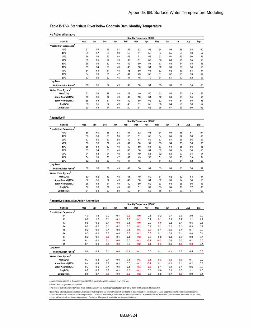
Oct Nov Dec Jan Feb Mar Apr May Jun Jul Aug Sep
10% 61 59 55 51 51 52 53 54 56 58 58 6020% 58 57 53 50 50 51 52 54 55 56 56 5730% 56 56 53 50 49 51 52 53 54 55 56 5640% 55 55 52 49 49 51 52 53 54 55 55 5650% 55 54 52 49 49 50 51 53 53 54 55 5560% 55 54 51 48 48 50 51 52 53 53 54 5570% 54 54 51 48 48 50 51 52 52 53 54 5480% 54 53 50 47 47 49 50 51 52 53 53 5490% 52 52 50 46 47 48 49 51 51 52 52 53
Full Simulation Periodb 56 55 52 49 49 50 51 53 53 55 55 56
Wet (32%) 52 52 49 48 48 49 50 52 52 53 53 53Above Normal (16%) 56 55 52 49 49 50 51 52 53 53 54 55Below Normal (13%) 55 54 51 49 49 50 52 52 53 54 55 56
Dry (24%) 56 55 52 49 49 51 52 53 54 55 56 57Critical (15%) 60 58 54 50 50 51 53 55 57 59 60 63
Oct Nov Dec Jan Feb Mar Apr May Jun Jul Aug Sep
10% 65 60 55 51 51 52 53 54 56 58 61 6420% 59 58 53 50 50 51 53 54 55 57 58 5930% 57 56 53 50 49 51 52 53 54 56 56 5740% 56 55 52 49 49 50 52 53 54 55 56 5650% 55 54 52 49 49 50 51 53 53 55 55 5560% 55 54 51 48 48 50 51 52 53 54 54 5570% 54 54 51 48 48 49 51 52 52 53 54 5480% 54 53 50 47 47 49 50 51 52 53 53 5490% 52 52 50 46 47 48 49 51 51 51 52 53
Full Simulation Periodb 57 55 52 49 49 50 51 53 53 55 56 57
Wet (32%) 53 52 49 48 48 49 50 51 52 52 53 54Above Normal (16%) 57 55 52 49 49 50 51 52 53 54 54 55Below Normal (13%) 56 54 51 49 49 50 52 53 53 55 56 56
Dry (24%) 56 55 52 49 49 51 52 53 54 56 57 58Critical (15%) 61 58 53 50 50 51 53 56 57 59 61 63
Oct Nov Dec Jan Feb Mar Apr May Jun Jul Aug Sep
0.1 4.0 1.3 0.2 0.1 -0.2 0.0 0.1 0.2 0.7 0.8 3.0 3.90.2 0.8 1.5 0.1 -0.1 0.0 -0.1 0.1 0.1 0.3 0.7 1.1 1.20.3 0.6 0.5 0.1 0.0 -0.1 0.0 0.0 0.0 0.2 0.4 0.5 0.60.4 0.2 0.2 0.1 -0.2 0.0 -0.1 0.2 0.1 0.1 0.1 0.3 0.20.5 0.2 0.2 0.1 0.0 -0.1 -0.1 0.0 0.1 -0.1 0.1 0.1 0.00.6 0.3 0.1 0.2 0.0 0.0 -0.1 0.0 0.1 0.0 0.1 0.0 0.10.7 0.2 0.1 -0.1 0.1 -0.1 -0.3 0.0 0.0 -0.3 0.0 0.0 0.10.8 0.1 0.1 0.1 0.0 0.0 -0.1 -0.1 -0.2 0.0 0.0 0.1 0.0
0.9 0.1 0.0 -0.1 -0.3 0.0 -0.2 -0.1 -0.1 -0.1 0.0 0.0 0.1
Full Simulation Periodb 0.6 0.4 0.1 0.0 -0.1 -0.1 0.0 0.1 -0.1 0.2 0.5 0.6
Wet (32%) 0.7 0.3 0.1 0.0 -0.1 -0.1 -0.1 -0.1 -0.1 0.0 0.1 0.2Above Normal (16%) 0.4 0.4 0.2 0.1 0.0 -0.1 -0.1 0.1 -0.1 0.1 0.2 0.3Below Normal (13%) 0.7 0.0 0.1 0.0 -0.1 -0.1 0.0 0.1 0.2 0.4 0.6 0.8
Dry (24%) 0.7 0.5 0.2 0.1 0.0 -0.1 0.0 0.0 0.2 0.5 1.1 1.6Critical (15%) 0.5 0.7 -0.1 -0.2 -0.3 -0.2 0.5 0.8 -0.7 0.0 0.9 0.4
a Exceedance probability is defined as the probability a given value will be exceeded in any one year.
b Based on an 81-year simulation period.
Probability of Exceedancea
Long Term
Water Year Typesc
c As defined by the Sacramento Valley 40-30-30 Index Water Year Hydrologic Classification (SWRCB D-1641, 1999); projected to Year 2030.
Notes: 1) All alternatives are simulated with projected hydrology and sea level at Year 2030 conditions. 2) Model results for Alternatives 1, 4, and Second Basis of Comparison are the same,
therefore Alternative 1 and 4 results are not presented. Qualitative differences, if applicable, are discussed in the text. 3) Model results for Alternative 2 and No Action Alternative are the same,
therefore Alternative 2 results are not presented. Qualitative differences, if applicable, are discussed in the text.
Probability of Exceedancea
Long Term
Water Year Typesc
Alternative 5 minus No Action Alternative
Statistic
Monthly Temperature (DEG-F)
Long Term
Water Year Typesc
Alternative 5
Statistic
Monthly Temperature (DEG-F)
No Action Alternative
Statistic
Monthly Temperature (DEG-F)
Probability of Exceedancea
Table B-17-3. Stanislaus River below Goodwin Dam, Monthly Temperature
Appendix 6B: Surface Water Temperature Modeling
6B.B-324

Oct Nov Dec Jan Feb Mar Apr May Jun Jul Aug Sep
10% 60 59 55 51 51 52 53 54 56 57 58 5920% 57 56 53 50 50 51 52 54 55 56 56 5730% 56 55 53 50 50 51 52 53 54 55 56 5640% 56 55 52 49 49 51 52 53 54 55 55 5650% 55 54 52 49 49 50 51 53 53 54 55 5560% 55 54 51 49 49 50 51 52 53 53 54 5570% 54 53 51 48 48 50 51 52 52 53 54 5480% 54 53 51 48 48 49 50 51 52 52 53 5490% 53 52 50 47 47 48 49 51 51 51 52 52
Full Simulation Periodb 56 55 52 49 49 50 51 53 53 54 55 56
Wet (32%) 52 52 49 48 48 49 50 52 52 52 53 53Above Normal (16%) 56 55 52 49 49 50 51 52 53 53 54 55Below Normal (13%) 55 54 51 49 49 50 51 53 53 54 55 55
Dry (24%) 56 55 52 49 49 51 52 53 54 55 56 57Critical (15%) 60 58 54 50 50 52 53 55 56 59 60 61
Oct Nov Dec Jan Feb Mar Apr May Jun Jul Aug Sep
10% 61 59 55 51 51 52 53 54 56 58 58 6020% 58 57 53 50 50 51 52 54 55 56 56 5730% 56 56 53 50 49 51 52 53 54 55 56 5640% 55 55 52 49 49 51 52 53 54 55 55 5650% 55 54 52 49 49 50 51 53 53 54 55 5560% 55 54 51 48 48 50 51 52 53 53 54 5570% 54 54 51 48 48 50 51 52 52 53 54 5480% 54 53 50 47 47 49 50 51 52 53 53 5490% 52 52 50 46 47 48 49 51 51 52 52 53
Full Simulation Periodb 56 55 52 49 49 50 51 53 53 55 55 56
Wet (32%) 52 52 49 48 48 49 50 52 52 53 53 53Above Normal (16%) 56 55 52 49 49 50 51 52 53 53 54 55Below Normal (13%) 55 54 51 49 49 50 52 52 53 54 55 56
Dry (24%) 56 55 52 49 49 51 52 53 54 55 56 57Critical (15%) 60 58 54 50 50 51 53 55 57 59 60 63
Oct Nov Dec Jan Feb Mar Apr May Jun Jul Aug Sep
0.1 0.5 0.1 0.1 0.0 0.0 0.0 0.0 -0.1 0.1 0.2 0.2 0.90.2 0.7 0.1 0.0 0.0 -0.1 0.0 0.0 0.0 0.0 -0.1 0.1 0.40.3 -0.3 0.1 -0.2 -0.1 -0.1 -0.1 0.1 -0.2 0.1 0.2 0.1 0.20.4 -0.2 0.1 -0.1 0.0 -0.2 -0.1 0.0 -0.1 0.0 0.1 0.0 0.10.5 -0.3 -0.1 -0.1 -0.1 0.0 -0.1 0.0 0.0 0.0 0.2 0.1 0.10.6 -0.3 -0.1 -0.2 -0.1 -0.2 -0.1 -0.1 -0.1 -0.3 0.1 0.1 0.0
0.7 -0.5 0.0 -0.1 -0.2 -0.1 -0.1 -0.1 -0.1 0.0 0.1 0.1 0.10.8 -0.3 0.0 -0.1 -0.3 -0.3 -0.1 -0.1 0.0 0.0 0.2 -0.1 0.0
0.9 -0.3 -0.1 0.0 -0.4 -0.1 0.0 -0.1 0.0 -0.3 0.3 0.0 0.3
Full Simulation Periodb
0.0 0.0 -0.1 -0.1 -0.1 -0.1 0.0 -0.1 0.1 0.2 0.1 0.3
Wet (32%) -0.1 0.1 0.0 -0.1 -0.1 -0.1 -0.1 -0.1 -0.3 0.2 0.0 0.0
Above Normal (16%) -0.1 0.0 -0.1 -0.1 -0.1 -0.1 0.0 -0.2 0.0 0.1 0.1 0.1Below Normal (13%) 0.0 0.2 0.0 -0.1 -0.1 -0.1 0.2 -0.2 0.1 0.2 0.2 0.2
Dry (24%) -0.1 0.1 -0.1 -0.1 -0.1 -0.1 -0.1 -0.1 0.1 0.1 0.1 0.3Critical (15%) 0.4 -0.7 -0.4 -0.2 -0.2 -0.2 0.0 -0.1 0.8 0.3 -0.1 1.3
a Exceedance probability is defined as the probability a given value will be exceeded in any one year.
b Based on an 81-year simulation period.
Probability of Exceedancea
Long Term
Water Year Typesc
c As defined by the Sacramento Valley 40-30-30 Index Water Year Hydrologic Classification (SWRCB D-1641, 1999); projected to Year 2030.
Notes: 1) All alternatives are simulated with projected hydrology and sea level at Year 2030 conditions. 2) Model results for Alternatives 1, 4, and Second Basis of Comparison are the same,
therefore Alternative 1 and 4 results are not presented. Qualitative differences, if applicable, are discussed in the text. 3) Model results for Alternative 2 and No Action Alternative are the same,
therefore Alternative 2 results are not presented. Qualitative differences, if applicable, are discussed in the text.
Probability of Exceedancea
Long Term
Water Year Typesc
No Action Alternative minus Second Basis of Comparison
Statistic
Monthly Temperature (DEG-F)
Long Term
Water Year Typesc
No Action Alternative
Statistic
Monthly Temperature (DEG-F)
Second Basis of Comparison
Statistic
Monthly Temperature (DEG-F)
Probability of Exceedancea
Table B-17-4. Stanislaus River below Goodwin Dam, Monthly Temperature
Appendix 6B: Surface Water Temperature Modeling
6B.B-325

Oct Nov Dec Jan Feb Mar Apr May Jun Jul Aug Sep
10% 60 59 55 51 51 52 53 54 56 57 58 5920% 57 56 53 50 50 51 52 54 55 56 56 5730% 56 55 53 50 50 51 52 53 54 55 56 5640% 56 55 52 49 49 51 52 53 54 55 55 5650% 55 54 52 49 49 50 51 53 53 54 55 5560% 55 54 51 49 49 50 51 52 53 53 54 5570% 54 53 51 48 48 50 51 52 52 53 54 5480% 54 53 51 48 48 49 50 51 52 52 53 5490% 53 52 50 47 47 48 49 51 51 51 52 52
Full Simulation Periodb 56 55 52 49 49 50 51 53 53 54 55 56
Wet (32%) 52 52 49 48 48 49 50 52 52 52 53 53Above Normal (16%) 56 55 52 49 49 50 51 52 53 53 54 55Below Normal (13%) 55 54 51 49 49 50 51 53 53 54 55 55
Dry (24%) 56 55 52 49 49 51 52 53 54 55 56 57Critical (15%) 60 58 54 50 50 52 53 55 56 59 60 61
Oct Nov Dec Jan Feb Mar Apr May Jun Jul Aug Sep
10% 59 58 54 51 51 52 53 54 55 57 57 5820% 57 56 53 50 50 51 52 53 55 56 56 5730% 56 55 53 50 49 51 52 53 54 55 55 5640% 55 54 52 49 49 51 52 53 53 54 55 5550% 55 54 51 49 49 50 51 52 53 54 55 5560% 55 54 51 49 48 50 51 52 53 54 54 5470% 54 53 51 48 48 50 51 52 52 53 54 5480% 53 53 50 48 48 49 50 51 52 53 53 5390% 53 52 50 47 47 49 50 51 51 52 52 52
Full Simulation Periodb 55 55 52 49 49 50 51 52 53 54 55 55
Wet (32%) 52 51 49 48 48 50 50 51 52 53 53 53Above Normal (16%) 56 55 52 49 49 50 51 52 53 54 54 54Below Normal (13%) 55 54 51 49 49 50 51 52 53 54 55 55
Dry (24%) 55 54 52 49 49 51 52 53 54 55 55 56Critical (15%) 59 57 54 50 50 52 53 54 56 58 60 60
Oct Nov Dec Jan Feb Mar Apr May Jun Jul Aug Sep
0.1 -1.7 -1.4 -0.4 -0.1 0.0 0.2 0.0 -0.2 -0.2 -0.7 -0.9 -0.9
0.2 -0.3 -0.5 0.1 -0.3 -0.1 0.0 0.1 -0.1 -0.2 -0.3 -0.4 -0.4
0.3 -0.4 -0.7 0.1 -0.1 -0.1 0.0 0.0 -0.3 0.0 -0.2 -0.3 -0.3
0.4 -0.5 -0.4 -0.3 -0.2 0.0 0.0 0.0 -0.2 -0.1 -0.1 -0.4 -0.4
0.5 -0.4 -0.5 -0.2 -0.1 0.0 0.1 0.0 -0.2 -0.1 -0.2 -0.2 -0.3
0.6 -0.3 -0.4 -0.2 0.1 -0.1 -0.1 0.0 -0.1 -0.2 0.2 0.0 -0.2
0.7 -0.4 -0.2 -0.2 -0.1 0.0 0.0 0.1 -0.1 0.0 0.3 -0.1 -0.3
0.8 -0.5 -0.1 -0.1 0.1 0.0 -0.1 0.0 -0.1 0.0 0.4 -0.3 -0.4
0.9 -0.1 -0.1 -0.1 0.3 0.1 0.2 0.3 0.0 0.2 0.6 0.2 0.1
Full Simulation Periodb
-0.5 -0.4 -0.1 -0.1 0.0 0.0 0.0 -0.3 -0.1 0.0 -0.3 -0.5
Wet (32%) -0.3 -0.2 -0.1 0.0 0.2 0.1 0.1 -0.1 -0.1 0.5 0.0 -0.2
Above Normal (16%) -0.5 -0.4 -0.2 0.0 0.0 0.0 0.1 -0.1 0.1 0.2 -0.1 -0.3
Below Normal (13%) -0.7 -0.5 -0.2 -0.1 -0.1 0.0 0.0 -0.3 0.1 -0.1 -0.2 -0.3
Dry (24%) -0.3 -0.3 -0.1 -0.1 -0.1 0.0 0.0 -0.1 -0.1 -0.2 -0.5 -0.7
Critical (15%) -1.3 -0.8 -0.2 -0.1 0.0 0.1 0.0 -0.8 -0.4 -0.6 -0.9 -1.5
a Exceedance probability is defined as the probability a given value will be exceeded in any one year.
b Based on an 81-year simulation period.
Probability of Exceedancea
Long Term
Water Year Typesc
c As defined by the Sacramento Valley 40-30-30 Index Water Year Hydrologic Classification (SWRCB D-1641, 1999); projected to Year 2030.
Notes: 1) All alternatives are simulated with projected hydrology and sea level at Year 2030 conditions. 2) Model results for Alternatives 1, 4, and Second Basis of Comparison are the same,
therefore Alternative 1 and 4 results are not presented. Qualitative differences, if applicable, are discussed in the text. 3) Model results for Alternative 2 and No Action Alternative are the same,
therefore Alternative 2 results are not presented. Qualitative differences, if applicable, are discussed in the text.
Probability of Exceedancea
Long Term
Water Year Typesc
Alternative 3 minus Second Basis of Comparison
Statistic
Monthly Temperature (DEG-F)
Long Term
Water Year Typesc
Alternative 3
Statistic
Monthly Temperature (DEG-F)
Second Basis of Comparison
Statistic
Monthly Temperature (DEG-F)
Probability of Exceedancea
Final LTO EIS6B.B-326
Table B-17-5. Stanislaus River below Goodwin Dam, Monthly Temperature
Appendix 6B: Surface Water Temperature Modeling

Oct Nov Dec Jan Feb Mar Apr May Jun Jul Aug Sep
10% 60 59 55 51 51 52 53 54 56 57 58 5920% 57 56 53 50 50 51 52 54 55 56 56 5730% 56 55 53 50 50 51 52 53 54 55 56 5640% 56 55 52 49 49 51 52 53 54 55 55 5650% 55 54 52 49 49 50 51 53 53 54 55 5560% 55 54 51 49 49 50 51 52 53 53 54 5570% 54 53 51 48 48 50 51 52 52 53 54 5480% 54 53 51 48 48 49 50 51 52 52 53 5490% 53 52 50 47 47 48 49 51 51 51 52 52
Full Simulation Periodb 56 55 52 49 49 50 51 53 53 54 55 56
Wet (32%) 52 52 49 48 48 49 50 52 52 52 53 53Above Normal (16%) 56 55 52 49 49 50 51 52 53 53 54 55Below Normal (13%) 55 54 51 49 49 50 51 53 53 54 55 55
Dry (24%) 56 55 52 49 49 51 52 53 54 55 56 57Critical (15%) 60 58 54 50 50 52 53 55 56 59 60 61
Oct Nov Dec Jan Feb Mar Apr May Jun Jul Aug Sep
10% 65 60 55 51 51 52 53 54 56 58 61 6420% 59 58 53 50 50 51 53 54 55 57 58 5930% 57 56 53 50 49 51 52 53 54 56 56 5740% 56 55 52 49 49 50 52 53 54 55 56 5650% 55 54 52 49 49 50 51 53 53 55 55 5560% 55 54 51 48 48 50 51 52 53 54 54 5570% 54 54 51 48 48 49 51 52 52 53 54 5480% 54 53 50 47 47 49 50 51 52 53 53 5490% 52 52 50 46 47 48 49 51 51 51 52 53
Full Simulation Periodb 57 55 52 49 49 50 51 53 53 55 56 57
Wet (32%) 53 52 49 48 48 49 50 51 52 52 53 54Above Normal (16%) 57 55 52 49 49 50 51 52 53 54 54 55Below Normal (13%) 56 54 51 49 49 50 52 53 53 55 56 56
Dry (24%) 56 55 52 49 49 51 52 53 54 56 57 58Critical (15%) 61 58 53 50 50 51 53 56 57 59 61 63
Oct Nov Dec Jan Feb Mar Apr May Jun Jul Aug Sep
0.1 4.5 1.4 0.3 0.1 -0.2 -0.1 0.1 0.1 0.8 1.0 3.2 4.80.2 1.4 1.6 0.1 -0.1 -0.1 -0.1 0.2 0.1 0.3 0.6 1.2 1.70.3 0.3 0.6 -0.1 -0.1 -0.1 -0.1 0.2 -0.2 0.3 0.6 0.6 0.70.4 0.0 0.2 -0.1 -0.2 -0.2 -0.2 0.1 0.0 0.2 0.1 0.4 0.30.5 0.0 0.1 0.0 -0.1 -0.1 -0.2 0.0 0.0 0.0 0.3 0.2 0.10.6 -0.1 0.0 0.0 -0.1 -0.2 -0.2 -0.1 0.0 -0.2 0.2 0.1 0.10.7 -0.3 0.2 -0.2 -0.2 -0.3 -0.3 -0.1 -0.1 -0.3 0.1 0.1 0.20.8 -0.2 0.0 0.0 -0.3 -0.3 -0.2 -0.2 -0.2 0.0 0.2 0.0 -0.1
0.9 -0.2 -0.1 -0.2 -0.7 -0.1 -0.2 -0.2 -0.1 -0.5 0.2 0.0 0.4
Full Simulation Periodb 0.6 0.4 0.0 -0.1 -0.2 -0.2 0.0 0.0 0.0 0.4 0.6 1.0
Wet (32%) 0.6 0.4 0.1 -0.1 -0.2 -0.2 -0.2 -0.1 -0.4 0.2 0.1 0.2Above Normal (16%) 0.3 0.4 0.1 0.0 -0.1 -0.1 -0.1 -0.1 -0.1 0.2 0.3 0.4Below Normal (13%) 0.7 0.2 0.1 -0.1 -0.2 -0.2 0.1 -0.1 0.3 0.5 0.8 1.0
Dry (24%) 0.5 0.5 0.1 0.0 -0.1 -0.1 -0.1 0.0 0.2 0.6 1.2 1.9Critical (15%) 0.8 0.0 -0.5 -0.4 -0.5 -0.4 0.5 0.7 0.1 0.3 0.8 1.7
a Exceedance probability is defined as the probability a given value will be exceeded in any one year.
b Based on an 81-year simulation period.
Probability of Exceedancea
Long Term
Water Year Typesc
c As defined by the Sacramento Valley 40-30-30 Index Water Year Hydrologic Classification (SWRCB D-1641, 1999); projected to Year 2030.
Notes: 1) All alternatives are simulated with projected hydrology and sea level at Year 2030 conditions. 2) Model results for Alternatives 1, 4, and Second Basis of Comparison are the same,
therefore Alternative 1 and 4 results are not presented. Qualitative differences, if applicable, are discussed in the text. 3) Model results for Alternative 2 and No Action Alternative are the same,
therefore Alternative 2 results are not presented. Qualitative differences, if applicable, are discussed in the text.
Probability of Exceedancea
Long Term
Water Year Typesc
Alternative 5 minus Second Basis of Comparison
Statistic
Monthly Temperature (DEG-F)
Long Term
Water Year Typesc
Alternative 5
Statistic
Monthly Temperature (DEG-F)
Second Basis of Comparison
Statistic
Monthly Temperature (DEG-F)
Probability of Exceedancea
Final LTO EIS6B.B-327
Table B-17-6. Stanislaus River below Goodwin Dam, Monthly Temperature
Appendix 6B: Surface Water Temperature Modeling

B.18. Stanislaus River at Orange Blossom Bridge Temperature
Appendix 6B: Surface Water Temperature Modeling
6B.B-328

Figure B-18-1. Stanislaus River at Orange Blossom Bridge, October
Notes: 1) Exceedance probability is defined as the probability a given value will be exceeded in any one year. 2) All alternatives are simulated with projected hydrology and
sea level at Year 2030 conditions. 3) Model results for Alternatives 1, 4, and Second Basis of Comparison are the same, therefore Alternatives 1 and 4 results are not
presented. Qualitative differences, if applicable, are discussed in the text. 4) Model results for Alternative 2 and No Action Alternative are the same, therefore Alternative 2
results are not presented. Qualitative differences, if applicable, are discussed in the text.
44
46
48
50
52
54
56
58
60
62
64
66
68
70
72
74
76
0%10%20%30%40%50%60%70%80%90%100%
Exceedance Probability
No Action Alternative & Alternative 2 Second Basis of Comparison, Alternative 1, & Alternative 4
Alternative 3 Alternative 5
Mon
thly
Tem
pera
ture
(DE
G-F
)
Appendix 6B: Surface Water Temperature Modeling
6B.B-329

Figure B-18-2. Stanislaus River at Orange Blossom Bridge, November
Notes: 1) Exceedance probability is defined as the probability a given value will be exceeded in any one year. 2) All alternatives are simulated with projected hydrology and
sea level at Year 2030 conditions. 3) Model results for Alternatives 1, 4, and Second Basis of Comparison are the same, therefore Alternatives 1 and 4 results are not
presented. Qualitative differences, if applicable, are discussed in the text. 4) Model results for Alternative 2 and No Action Alternative are the same, therefore Alternative 2
results are not presented. Qualitative differences, if applicable, are discussed in the text.
44
46
48
50
52
54
56
58
60
62
64
66
68
70
72
74
76
0%10%20%30%40%50%60%70%80%90%100%
Exceedance Probability
No Action Alternative & Alternative 2 Second Basis of Comparison, Alternative 1, & Alternative 4
Alternative 3 Alternative 5
Mon
thly
Tem
pera
ture
(DE
G-F
)
Appendix 6B: Surface Water Temperature Modeling
6B.B-330

Figure B-18-3. Stanislaus River at Orange Blossom Bridge, December
Notes: 1) Exceedance probability is defined as the probability a given value will be exceeded in any one year. 2) All alternatives are simulated with projected hydrology and
sea level at Year 2030 conditions. 3) Model results for Alternatives 1, 4, and Second Basis of Comparison are the same, therefore Alternatives 1 and 4 results are not
presented. Qualitative differences, if applicable, are discussed in the text. 4) Model results for Alternative 2 and No Action Alternative are the same, therefore Alternative 2
results are not presented. Qualitative differences, if applicable, are discussed in the text.
44
46
48
50
52
54
56
58
60
62
64
66
68
70
72
74
76
0%10%20%30%40%50%60%70%80%90%100%
Exceedance Probability
No Action Alternative & Alternative 2 Second Basis of Comparison, Alternative 1, & Alternative 4
Alternative 3 Alternative 5
Mon
thly
Tem
pera
ture
(DE
G-F
)
Appendix 6B: Surface Water Temperature Modeling
6B.B-331

Figure B-18-4. Stanislaus River at Orange Blossom Bridge, January
Notes: 1) Exceedance probability is defined as the probability a given value will be exceeded in any one year. 2) All alternatives are simulated with projected hydrology and
sea level at Year 2030 conditions. 3) Model results for Alternatives 1, 4, and Second Basis of Comparison are the same, therefore Alternatives 1 and 4 results are not
presented. Qualitative differences, if applicable, are discussed in the text. 4) Model results for Alternative 2 and No Action Alternative are the same, therefore Alternative 2
results are not presented. Qualitative differences, if applicable, are discussed in the text.
44
46
48
50
52
54
56
58
60
62
64
66
68
70
72
74
76
0%10%20%30%40%50%60%70%80%90%100%
Exceedance Probability
No Action Alternative & Alternative 2 Second Basis of Comparison, Alternative 1, & Alternative 4
Alternative 3 Alternative 5
Mon
thly
Tem
pera
ture
(DE
G-F
)
Appendix 6B: Surface Water Temperature Modeling
6B.B-332

Figure B-18-5. Stanislaus River at Orange Blossom Bridge, February
Notes: 1) Exceedance probability is defined as the probability a given value will be exceeded in any one year. 2) All alternatives are simulated with projected hydrology and
sea level at Year 2030 conditions. 3) Model results for Alternatives 1, 4, and Second Basis of Comparison are the same, therefore Alternatives 1 and 4 results are not
presented. Qualitative differences, if applicable, are discussed in the text. 4) Model results for Alternative 2 and No Action Alternative are the same, therefore Alternative 2
results are not presented. Qualitative differences, if applicable, are discussed in the text.
44
46
48
50
52
54
56
58
60
62
64
66
68
70
72
74
76
0%10%20%30%40%50%60%70%80%90%100%
Exceedance Probability
No Action Alternative & Alternative 2 Second Basis of Comparison, Alternative 1, & Alternative 4
Alternative 3 Alternative 5
Mon
thly
Tem
pera
ture
(DE
G-F
)
Appendix 6B: Surface Water Temperature Modeling
6B.B-333

Figure B-18-6. Stanislaus River at Orange Blossom Bridge, March
Notes: 1) Exceedance probability is defined as the probability a given value will be exceeded in any one year. 2) All alternatives are simulated with projected hydrology and
sea level at Year 2030 conditions. 3) Model results for Alternatives 1, 4, and Second Basis of Comparison are the same, therefore Alternatives 1 and 4 results are not
presented. Qualitative differences, if applicable, are discussed in the text. 4) Model results for Alternative 2 and No Action Alternative are the same, therefore Alternative 2
results are not presented. Qualitative differences, if applicable, are discussed in the text.
44
46
48
50
52
54
56
58
60
62
64
66
68
70
72
74
76
0%10%20%30%40%50%60%70%80%90%100%
Exceedance Probability
No Action Alternative & Alternative 2 Second Basis of Comparison, Alternative 1, & Alternative 4
Alternative 3 Alternative 5
Mon
thly
Tem
pera
ture
(DE
G-F
)
Appendix 6B: Surface Water Temperature Modeling
6B.B-334

Figure B-18-7. Stanislaus River at Orange Blossom Bridge, April
Notes: 1) Exceedance probability is defined as the probability a given value will be exceeded in any one year. 2) All alternatives are simulated with projected hydrology and
sea level at Year 2030 conditions. 3) Model results for Alternatives 1, 4, and Second Basis of Comparison are the same, therefore Alternatives 1 and 4 results are not
presented. Qualitative differences, if applicable, are discussed in the text. 4) Model results for Alternative 2 and No Action Alternative are the same, therefore Alternative 2
results are not presented. Qualitative differences, if applicable, are discussed in the text.
44
46
48
50
52
54
56
58
60
62
64
66
68
70
72
74
76
0%10%20%30%40%50%60%70%80%90%100%
Exceedance Probability
No Action Alternative & Alternative 2 Second Basis of Comparison, Alternative 1, & Alternative 4
Alternative 3 Alternative 5
Mon
thly
Tem
pera
ture
(DE
G-F
)
Appendix 6B: Surface Water Temperature Modeling
6B.B-335

Figure B-18-8. Stanislaus River at Orange Blossom Bridge, May
Notes: 1) Exceedance probability is defined as the probability a given value will be exceeded in any one year. 2) All alternatives are simulated with projected hydrology and
sea level at Year 2030 conditions. 3) Model results for Alternatives 1, 4, and Second Basis of Comparison are the same, therefore Alternatives 1 and 4 results are not
presented. Qualitative differences, if applicable, are discussed in the text. 4) Model results for Alternative 2 and No Action Alternative are the same, therefore Alternative 2
results are not presented. Qualitative differences, if applicable, are discussed in the text.
44
46
48
50
52
54
56
58
60
62
64
66
68
70
72
74
76
0%10%20%30%40%50%60%70%80%90%100%
Exceedance Probability
No Action Alternative & Alternative 2 Second Basis of Comparison, Alternative 1, & Alternative 4
Alternative 3 Alternative 5
Mon
thly
Tem
pera
ture
(DE
G-F
)
Appendix 6B: Surface Water Temperature Modeling
6B.B-336

Figure B-18-9. Stanislaus River at Orange Blossom Bridge, June
Notes: 1) Exceedance probability is defined as the probability a given value will be exceeded in any one year. 2) All alternatives are simulated with projected hydrology and
sea level at Year 2030 conditions. 3) Model results for Alternatives 1, 4, and Second Basis of Comparison are the same, therefore Alternatives 1 and 4 results are not
presented. Qualitative differences, if applicable, are discussed in the text. 4) Model results for Alternative 2 and No Action Alternative are the same, therefore Alternative 2
results are not presented. Qualitative differences, if applicable, are discussed in the text.
44
46
48
50
52
54
56
58
60
62
64
66
68
70
72
74
76
0%10%20%30%40%50%60%70%80%90%100%
Exceedance Probability
No Action Alternative & Alternative 2 Second Basis of Comparison, Alternative 1, & Alternative 4
Alternative 3 Alternative 5
Mon
thly
Tem
pera
ture
(DE
G-F
)
Appendix 6B: Surface Water Temperature Modeling
6B.B-337
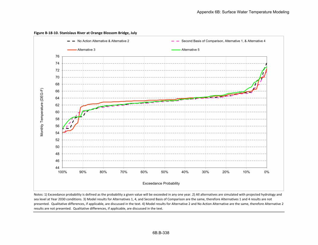
Figure B-18-10. Stanislaus River at Orange Blossom Bridge, July
Notes: 1) Exceedance probability is defined as the probability a given value will be exceeded in any one year. 2) All alternatives are simulated with projected hydrology and
sea level at Year 2030 conditions. 3) Model results for Alternatives 1, 4, and Second Basis of Comparison are the same, therefore Alternatives 1 and 4 results are not
presented. Qualitative differences, if applicable, are discussed in the text. 4) Model results for Alternative 2 and No Action Alternative are the same, therefore Alternative 2
results are not presented. Qualitative differences, if applicable, are discussed in the text.
44
46
48
50
52
54
56
58
60
62
64
66
68
70
72
74
76
0%10%20%30%40%50%60%70%80%90%100%
Exceedance Probability
No Action Alternative & Alternative 2 Second Basis of Comparison, Alternative 1, & Alternative 4
Alternative 3 Alternative 5
Mon
thly
Tem
pera
ture
(DE
G-F
)
Appendix 6B: Surface Water Temperature Modeling
6B.B-338

Figure B-18-11. Stanislaus River at Orange Blossom Bridge, August
Notes: 1) Exceedance probability is defined as the probability a given value will be exceeded in any one year. 2) All alternatives are simulated with projected hydrology and
sea level at Year 2030 conditions. 3) Model results for Alternatives 1, 4, and Second Basis of Comparison are the same, therefore Alternatives 1 and 4 results are not
presented. Qualitative differences, if applicable, are discussed in the text. 4) Model results for Alternative 2 and No Action Alternative are the same, therefore Alternative 2
results are not presented. Qualitative differences, if applicable, are discussed in the text.
44
46
48
50
52
54
56
58
60
62
64
66
68
70
72
74
76
0%10%20%30%40%50%60%70%80%90%100%
Exceedance Probability
No Action Alternative & Alternative 2 Second Basis of Comparison, Alternative 1, & Alternative 4
Alternative 3 Alternative 5
Mon
thly
Tem
pera
ture
(DE
G-F
)
Appendix 6B: Surface Water Temperature Modeling
6B.B-339

Figure B-18-12. Stanislaus River at Orange Blossom Bridge, September
Notes: 1) Exceedance probability is defined as the probability a given value will be exceeded in any one year. 2) All alternatives are simulated with projected hydrology and
sea level at Year 2030 conditions. 3) Model results for Alternatives 1, 4, and Second Basis of Comparison are the same, therefore Alternatives 1 and 4 results are not
presented. Qualitative differences, if applicable, are discussed in the text. 4) Model results for Alternative 2 and No Action Alternative are the same, therefore Alternative 2
results are not presented. Qualitative differences, if applicable, are discussed in the text.
44
46
48
50
52
54
56
58
60
62
64
66
68
70
72
74
76
0%10%20%30%40%50%60%70%80%90%100%
Exceedance Probability
No Action Alternative & Alternative 2 Second Basis of Comparison, Alternative 1, & Alternative 4
Alternative 3 Alternative 5
Mon
thly
Tem
pera
ture
(DE
G-F
)
Appendix 6B: Surface Water Temperature Modeling
6B.B-340
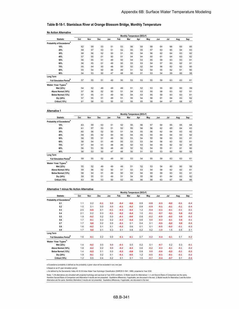
Oct Nov Dec Jan Feb Mar Apr May Jun Jul Aug Sep
10% 62 59 53 51 53 56 55 58 64 66 65 6520% 59 57 53 51 52 55 55 57 63 65 64 6330% 58 56 52 50 51 55 54 56 62 64 63 6240% 57 55 51 50 51 54 54 55 61 64 63 6250% 56 55 51 49 50 54 53 55 59 63 63 6160% 56 55 51 49 50 53 53 54 57 63 62 6170% 55 54 50 48 50 52 52 54 56 62 62 6080% 55 54 50 48 49 51 52 54 55 62 61 6090% 54 53 50 47 48 50 51 53 54 59 60 58
Full Simulation Periodb 57 55 51 49 50 53 53 55 59 63 63 61
Wet (32%) 54 52 49 49 49 51 52 53 55 60 60 59Above Normal (16%) 57 56 52 50 51 54 53 55 58 63 62 61Below Normal (13%) 57 55 51 49 50 54 53 55 59 63 63 61
Dry (24%) 57 55 51 49 51 55 54 56 61 64 63 62Critical (15%) 61 58 53 50 52 55 55 58 64 67 68 67
Oct Nov Dec Jan Feb Mar Apr May Jun Jul Aug Sep
10% 63 59 53 51 52 55 56 57 64 65 65 6420% 61 57 53 51 52 55 56 56 62 65 64 6330% 60 56 52 50 51 54 55 56 62 64 63 6240% 59 55 52 50 50 54 55 55 60 64 63 6250% 58 55 51 49 50 53 54 55 58 63 63 6160% 58 54 51 49 50 53 53 54 56 63 62 6170% 57 54 51 48 49 52 53 54 55 62 62 6080% 56 53 50 48 49 52 52 54 55 61 61 6090% 56 53 50 47 48 50 51 53 53 60 60 58
Full Simulation Periodb 59 55 52 49 50 53 54 55 59 63 63 61
Wet (32%) 55 52 49 49 49 51 52 53 54 60 60 58Above Normal (16%) 59 56 52 50 51 53 53 54 58 62 62 61Below Normal (13%) 58 54 51 49 50 53 54 55 59 63 63 61
Dry (24%) 59 55 51 49 51 54 55 56 61 64 63 62Critical (15%) 63 58 53 50 52 55 56 58 63 67 68 66
Oct Nov Dec Jan Feb Mar Apr May Jun Jul Aug Sep
0.1 1.1 0.2 -0.1 0.0 -0.4 -0.5 0.9 -0.8 -0.3 -0.2 -0.1 -0.4
0.2 1.5 0.1 0.0 0.0 -0.1 -0.2 0.8 -0.9 -0.1 -0.1 -0.1 -0.4
0.3 2.5 -0.5 0.1 -0.1 -0.3 -0.3 1.2 -0.4 -0.1 -0.1 -0.1 -0.1
0.4 2.1 0.2 0.3 -0.1 -0.2 -0.4 1.0 -0.1 -0.7 -0.1 0.0 -0.2
0.5 1.9 -0.2 0.2 0.0 -0.1 -0.6 0.8 -0.2 -0.9 -0.2 0.0 -0.2
0.6 1.7 -0.1 0.3 0.2 -0.3 -0.4 0.6 0.0 -0.3 -0.1 0.0 -0.1
0.7 1.7 0.0 0.2 0.0 -0.1 0.1 0.4 0.1 -0.5 -0.2 0.0 -0.3
0.8 1.6 -0.2 0.1 0.1 -0.2 0.6 0.1 0.1 -0.5 -0.2 -0.1 -0.3
0.9 1.7 0.0 0.1 0.3 0.1 0.8 0.2 0.2 -1.0 1.5 0.5 0.1
Full Simulation Periodb 1.6 -0.1 0.2 0.0 -0.1 -0.1 0.7 -0.2 -0.4 -0.1 0.1 -0.2
Wet (32%) 1.4 -0.2 0.0 0.0 -0.1 0.5 0.2 0.1 -0.7 0.2 0.3 -0.1
Above Normal (16%) 1.8 -0.2 0.2 0.0 -0.2 -0.3 0.6 -0.2 -0.3 -0.1 -0.1 -0.2
Below Normal (13%) 1.4 -0.3 0.1 0.0 -0.3 -0.6 0.8 0.0 -0.6 -0.2 -0.1 -0.3
Dry (24%) 1.9 -0.1 0.2 0.1 -0.1 -0.5 1.2 -0.5 -0.1 -0.1 -0.1 -0.2
Critical (15%) 1.2 0.5 0.4 0.2 0.1 0.1 1.0 -0.7 -0.4 -0.7 0.1 -0.4
a Exceedance probability is defined as the probability a given value will be exceeded in any one year.
b Based on an 81-year simulation period.
Probability of Exceedancea
Long Term
Water Year Typesc
c As defined by the Sacramento Valley 40-30-30 Index Water Year Hydrologic Classification (SWRCB D-1641, 1999); projected to Year 2030.
Notes: 1) All alternatives are simulated with projected hydrology and sea level at Year 2030 conditions. 2) Model results for Alternatives 1, 4, and Second Basis of Comparison are the same,
therefore Second Basis of Comparison and Alternative 4 results are not presented. Qualitative differences, if applicable, are discussed in the text. 3) Model results for Alternative 2 and No Action
Alternative are the same, therefore Alternative 2 results are not presented. Qualitative differences, if applicable, are discussed in the text.
Probability of Exceedancea
Long Term
Water Year Typesc
Alternative 1 minus No Action Alternative
Statistic
Monthly Temperature (DEG-F)
Long Term
Water Year Typesc
Alternative 1
Statistic
Monthly Temperature (DEG-F)
No Action Alternative
Statistic
Monthly Temperature (DEG-F)
Probability of Exceedancea
Table B-18-1. Stanislaus River at Orange Blossom Bridge, Monthly Temperature
Appendix 6B: Surface Water Temperature Modeling
6B.B-341

Oct Nov Dec Jan Feb Mar Apr May Jun Jul Aug Sep
10% 62 59 53 51 53 56 55 58 64 66 65 6520% 59 57 53 51 52 55 55 57 63 65 64 6330% 58 56 52 50 51 55 54 56 62 64 63 6240% 57 55 51 50 51 54 54 55 61 64 63 6250% 56 55 51 49 50 54 53 55 59 63 63 6160% 56 55 51 49 50 53 53 54 57 63 62 6170% 55 54 50 48 50 52 52 54 56 62 62 6080% 55 54 50 48 49 51 52 54 55 62 61 6090% 54 53 50 47 48 50 51 53 54 59 60 58
Full Simulation Periodb 57 55 51 49 50 53 53 55 59 63 63 61
Wet (32%) 54 52 49 49 49 51 52 53 55 60 60 59Above Normal (16%) 57 56 52 50 51 54 53 55 58 63 62 61Below Normal (13%) 57 55 51 49 50 54 53 55 59 63 63 61
Dry (24%) 57 55 51 49 51 55 54 56 61 64 63 62Critical (15%) 61 58 53 50 52 55 55 58 64 67 68 67
Oct Nov Dec Jan Feb Mar Apr May Jun Jul Aug Sep
10% 61 58 53 51 53 56 55 58 64 66 65 6320% 60 57 53 51 52 55 55 57 63 65 64 6330% 59 55 52 50 51 55 54 56 63 64 63 6240% 58 55 52 50 51 54 54 56 62 64 63 6150% 58 54 51 49 50 54 53 55 62 63 62 6160% 57 54 51 49 50 53 53 55 61 63 62 6170% 57 54 50 48 50 53 52 54 61 63 62 6080% 56 54 50 48 49 52 52 54 60 63 62 6090% 55 53 50 47 48 51 51 53 59 61 60 56
Full Simulation Periodb 58 55 51 49 51 53 53 55 61 63 62 61
Wet (32%) 55 52 49 49 50 52 52 54 59 61 60 58Above Normal (16%) 59 55 52 50 51 53 53 55 62 63 62 61Below Normal (13%) 57 54 51 49 50 54 53 55 62 64 63 61
Dry (24%) 58 55 51 49 51 55 54 56 62 64 63 62Critical (15%) 61 58 53 50 52 55 56 58 64 67 67 65
Oct Nov Dec Jan Feb Mar Apr May Jun Jul Aug Sep
0.1 -0.3 -1.1 -0.3 -0.3 0.4 0.0 0.2 0.1 0.1 0.3 -0.6 -1.1
0.2 0.6 -0.4 0.0 -0.1 0.3 0.2 0.0 -0.1 0.6 0.2 -0.4 -0.7
0.3 1.6 -0.8 -0.1 0.1 0.1 0.0 0.2 0.3 1.0 0.1 -0.3 0.00.4 1.4 -0.2 0.1 0.0 0.2 0.1 0.2 0.3 1.4 0.2 -0.1 -0.2
0.5 1.5 -0.4 -0.1 0.0 0.1 0.0 0.2 0.2 2.4 0.3 -0.1 -0.1
0.6 1.6 -0.5 0.1 0.0 0.0 0.1 0.1 0.3 4.7 0.7 -0.1 0.00.7 1.6 -0.2 0.0 0.1 0.1 0.5 0.3 0.5 4.9 1.0 0.0 -0.1
0.8 1.5 -0.1 0.0 0.3 0.2 0.6 0.0 0.2 5.0 1.2 0.1 0.10.9 1.4 0.2 0.1 0.4 0.1 0.8 0.4 0.5 4.5 2.8 0.6 -2.3
Full Simulation Periodb 1.1 -0.4 0.0 0.1 0.2 0.3 0.2 0.2 2.3 0.4 -0.3 -0.6
Wet (32%) 1.1 -0.3 0.0 0.1 0.1 0.8 0.2 0.4 3.6 0.6 -0.2 -0.4
Above Normal (16%) 1.4 -0.4 0.0 0.2 0.0 -0.2 0.2 0.3 3.7 1.0 0.0 -0.1
Below Normal (13%) 0.9 -0.6 -0.2 0.0 -0.2 0.2 0.1 0.4 2.3 0.2 -0.2 -0.3
Dry (24%) 1.5 -0.3 0.1 0.0 0.3 0.1 0.2 0.3 1.1 0.2 -0.4 -0.6
Critical (15%) -0.1 -0.2 0.2 0.1 0.6 0.3 0.1 -0.3 0.3 -0.4 -1.0 -2.1
a Exceedance probability is defined as the probability a given value will be exceeded in any one year.
b Based on an 81-year simulation period.
Probability of Exceedancea
Long Term
Water Year Typesc
c As defined by the Sacramento Valley 40-30-30 Index Water Year Hydrologic Classification (SWRCB D-1641, 1999); projected to Year 2030.
Notes: 1) All alternatives are simulated with projected hydrology and sea level at Year 2030 conditions. 2) Model results for Alternatives 1, 4, and Second Basis of Comparison are the same,
therefore Alternative 1 and 4 results are not presented. Qualitative differences, if applicable, are discussed in the text. 3) Model results for Alternative 2 and No Action Alternative are the same,
therefore Alternative 2 results are not presented. Qualitative differences, if applicable, are discussed in the text.
Probability of Exceedancea
Long Term
Water Year Typesc
Alternative 3 minus No Action Alternative
Statistic
Monthly Temperature (DEG-F)
Long Term
Water Year Typesc
Alternative 3
Statistic
Monthly Temperature (DEG-F)
No Action Alternative
Statistic
Monthly Temperature (DEG-F)
Probability of Exceedancea
Table B-18-2. Stanislaus River at Orange Blossom Bridge, Monthly Temperature
Appendix 6B: Surface Water Temperature Modeling
6B.B-342

Oct Nov Dec Jan Feb Mar Apr May Jun Jul Aug Sep
10% 62 59 53 51 53 56 55 58 64 66 65 6520% 59 57 53 51 52 55 55 57 63 65 64 6330% 58 56 52 50 51 55 54 56 62 64 63 6240% 57 55 51 50 51 54 54 55 61 64 63 6250% 56 55 51 49 50 54 53 55 59 63 63 6160% 56 55 51 49 50 53 53 54 57 63 62 6170% 55 54 50 48 50 52 52 54 56 62 62 6080% 55 54 50 48 49 51 52 54 55 62 61 6090% 54 53 50 47 48 50 51 53 54 59 60 58
Full Simulation Periodb 57 55 51 49 50 53 53 55 59 63 63 61
Wet (32%) 54 52 49 49 49 51 52 53 55 60 60 59Above Normal (16%) 57 56 52 50 51 54 53 55 58 63 62 61Below Normal (13%) 57 55 51 49 50 54 53 55 59 63 63 61
Dry (24%) 57 55 51 49 51 55 54 56 61 64 63 62Critical (15%) 61 58 53 50 52 55 55 58 64 67 68 67
Oct Nov Dec Jan Feb Mar Apr May Jun Jul Aug Sep
10% 65 60 53 51 53 56 55 56 64 66 67 6720% 60 58 53 51 52 55 54 56 63 65 65 6430% 58 56 52 50 51 55 54 55 62 64 64 6340% 57 55 52 50 51 54 53 55 61 64 63 6250% 57 55 51 49 50 54 53 55 59 63 63 6160% 56 55 51 49 50 53 53 54 57 63 62 6170% 55 54 51 48 50 52 52 54 56 62 62 6180% 55 54 50 48 49 51 52 53 55 62 61 6090% 54 53 50 47 48 50 51 53 54 59 60 58
Full Simulation Periodb 58 56 51 49 50 53 53 55 59 63 63 62
Wet (32%) 54 53 49 49 49 51 51 53 55 60 61 59Above Normal (16%) 58 56 52 50 51 54 53 54 58 63 62 61Below Normal (13%) 57 55 51 49 50 54 53 55 60 64 63 62
Dry (24%) 58 56 51 49 51 55 54 55 62 64 64 63Critical (15%) 62 58 53 50 52 55 55 58 64 68 68 67
Oct Nov Dec Jan Feb Mar Apr May Jun Jul Aug Sep
0.1 3.4 0.9 -0.1 0.1 0.0 0.0 -0.6 -1.4 0.2 0.8 1.5 2.80.2 0.7 1.0 0.0 -0.2 0.0 -0.1 -0.7 -1.0 0.2 0.5 0.7 0.90.3 0.5 0.3 -0.1 -0.2 0.0 0.0 -0.4 -0.6 0.2 0.2 0.3 0.70.4 0.3 0.2 0.1 0.0 0.0 -0.1 -0.2 -0.3 0.3 0.0 0.1 0.20.5 0.1 0.1 0.0 0.0 0.0 -0.1 0.0 -0.3 -0.1 0.0 0.1 0.10.6 0.1 0.1 0.1 0.1 0.0 0.0 0.0 -0.1 0.4 0.1 0.0 0.10.7 0.2 0.2 0.1 0.1 0.0 -0.1 0.1 -0.2 0.0 0.1 0.1 0.10.8 0.1 0.1 0.1 0.0 0.0 0.0 0.0 -0.2 0.0 0.1 0.0 0.00.9 0.0 0.3 0.0 0.1 -0.1 0.0 -0.1 0.0 0.0 0.3 0.2 -0.1
Full Simulation Periodb 0.6 0.3 0.1 0.0 0.0 0.0 -0.3 -0.3 0.2 0.3 0.5 0.5
Wet (32%) 0.6 0.3 0.1 0.0 -0.1 0.0 0.0 -0.2 0.0 0.5 0.5 0.2Above Normal (16%) 0.4 0.3 0.1 0.1 0.0 0.0 -0.2 -0.4 -0.1 0.1 0.1 0.2Below Normal (13%) 0.7 0.0 0.0 0.0 0.0 -0.1 -0.2 -0.2 0.5 0.3 0.4 0.5
Dry (24%) 0.6 0.4 0.2 0.1 0.0 0.0 -0.5 -0.6 0.2 0.3 0.7 1.1Critical (15%) 0.4 0.6 0.0 -0.2 -0.1 -0.1 -0.6 -0.2 0.5 0.5 0.9 0.4
a Exceedance probability is defined as the probability a given value will be exceeded in any one year.
b Based on an 81-year simulation period.
Probability of Exceedancea
Long Term
Water Year Typesc
c As defined by the Sacramento Valley 40-30-30 Index Water Year Hydrologic Classification (SWRCB D-1641, 1999); projected to Year 2030.
Notes: 1) All alternatives are simulated with projected hydrology and sea level at Year 2030 conditions. 2) Model results for Alternatives 1, 4, and Second Basis of Comparison are the same,
therefore Alternative 1 and 4 results are not presented. Qualitative differences, if applicable, are discussed in the text. 3) Model results for Alternative 2 and No Action Alternative are the same,
therefore Alternative 2 results are not presented. Qualitative differences, if applicable, are discussed in the text.
Probability of Exceedancea
Long Term
Water Year Typesc
Alternative 5 minus No Action Alternative
Statistic
Monthly Temperature (DEG-F)
Long Term
Water Year Typesc
Alternative 5
Statistic
Monthly Temperature (DEG-F)
No Action Alternative
Statistic
Monthly Temperature (DEG-F)
Probability of Exceedancea
Table B-18-3. Stanislaus River at Orange Blossom Bridge, Monthly Temperature
Appendix 6B: Surface Water Temperature Modeling
6B.B-343

Oct Nov Dec Jan Feb Mar Apr May Jun Jul Aug Sep
10% 63 59 53 51 52 55 56 57 64 65 65 6420% 61 57 53 51 52 55 56 56 62 65 64 6330% 60 56 52 50 51 54 55 56 62 64 63 6240% 59 55 52 50 50 54 55 55 60 64 63 6250% 58 55 51 49 50 53 54 55 58 63 63 6160% 58 54 51 49 50 53 53 54 56 63 62 6170% 57 54 51 48 49 52 53 54 55 62 62 6080% 56 53 50 48 49 52 52 54 55 61 61 6090% 56 53 50 47 48 50 51 53 53 60 60 58
Full Simulation Periodb 59 55 52 49 50 53 54 55 59 63 63 61
Wet (32%) 55 52 49 49 49 51 52 53 54 60 60 58Above Normal (16%) 59 56 52 50 51 53 53 54 58 62 62 61Below Normal (13%) 58 54 51 49 50 53 54 55 59 63 63 61
Dry (24%) 59 55 51 49 51 54 55 56 61 64 63 62Critical (15%) 63 58 53 50 52 55 56 58 63 67 68 66
Oct Nov Dec Jan Feb Mar Apr May Jun Jul Aug Sep
10% 62 59 53 51 53 56 55 58 64 66 65 6520% 59 57 53 51 52 55 55 57 63 65 64 6330% 58 56 52 50 51 55 54 56 62 64 63 6240% 57 55 51 50 51 54 54 55 61 64 63 6250% 56 55 51 49 50 54 53 55 59 63 63 6160% 56 55 51 49 50 53 53 54 57 63 62 6170% 55 54 50 48 50 52 52 54 56 62 62 6080% 55 54 50 48 49 51 52 54 55 62 61 6090% 54 53 50 47 48 50 51 53 54 59 60 58
Full Simulation Periodb 57 55 51 49 50 53 53 55 59 63 63 61
Wet (32%) 54 52 49 49 49 51 52 53 55 60 60 59Above Normal (16%) 57 56 52 50 51 54 53 55 58 63 62 61Below Normal (13%) 57 55 51 49 50 54 53 55 59 63 63 61
Dry (24%) 57 55 51 49 51 55 54 56 61 64 63 62Critical (15%) 61 58 53 50 52 55 55 58 64 67 68 67
Oct Nov Dec Jan Feb Mar Apr May Jun Jul Aug Sep
0.1 -1.1 -0.2 0.1 0.0 0.4 0.5 -0.9 0.8 0.3 0.2 0.1 0.40.2 -1.5 -0.1 0.0 0.0 0.1 0.2 -0.8 0.9 0.1 0.1 0.1 0.40.3 -2.5 0.5 -0.1 0.1 0.3 0.3 -1.2 0.4 0.1 0.1 0.1 0.10.4 -2.1 -0.2 -0.3 0.1 0.2 0.4 -1.0 0.1 0.7 0.1 0.0 0.20.5 -1.9 0.2 -0.2 0.0 0.1 0.6 -0.8 0.2 0.9 0.2 0.0 0.20.6 -1.7 0.1 -0.3 -0.2 0.3 0.4 -0.6 0.0 0.3 0.1 0.0 0.10.7 -1.7 0.0 -0.2 0.0 0.1 -0.1 -0.4 -0.1 0.5 0.2 0.0 0.30.8 -1.6 0.2 -0.1 -0.1 0.2 -0.6 -0.1 -0.1 0.5 0.2 0.1 0.30.9 -1.7 0.0 -0.1 -0.3 -0.1 -0.8 -0.2 -0.2 1.0 -1.5 -0.5 -0.1
Full Simulation Periodb
-1.6 0.1 -0.2 0.0 0.1 0.1 -0.7 0.2 0.4 0.1 -0.1 0.2
Wet (32%) -1.4 0.2 0.0 0.0 0.1 -0.5 -0.2 -0.1 0.7 -0.2 -0.3 0.1Above Normal (16%) -1.8 0.2 -0.2 0.0 0.2 0.3 -0.6 0.2 0.3 0.1 0.1 0.2Below Normal (13%) -1.4 0.3 -0.1 0.0 0.3 0.6 -0.8 0.0 0.6 0.2 0.1 0.3
Dry (24%) -1.9 0.1 -0.2 -0.1 0.1 0.5 -1.2 0.5 0.1 0.1 0.1 0.2Critical (15%) -1.2 -0.5 -0.4 -0.2 -0.1 -0.1 -1.0 0.7 0.4 0.7 -0.1 0.4
a Exceedance probability is defined as the probability a given value will be exceeded in any one year.
b Based on an 81-year simulation period.
Probability of Exceedancea
Long Term
Water Year Typesc
c As defined by the Sacramento Valley 40-30-30 Index Water Year Hydrologic Classification (SWRCB D-1641, 1999); projected to Year 2030.
Notes: 1) All alternatives are simulated with projected hydrology and sea level at Year 2030 conditions. 2) Model results for Alternatives 1, 4, and Second Basis of Comparison are the same,
therefore Alternative 1 and 4 results are not presented. Qualitative differences, if applicable, are discussed in the text. 3) Model results for Alternative 2 and No Action Alternative are the same,
therefore Alternative 2 results are not presented. Qualitative differences, if applicable, are discussed in the text.
Probability of Exceedancea
Long Term
Water Year Typesc
No Action Alternative minus Second Basis of Comparison
Statistic
Monthly Temperature (DEG-F)
Long Term
Water Year Typesc
No Action Alternative
Statistic
Monthly Temperature (DEG-F)
Second Basis of Comparison
Statistic
Monthly Temperature (DEG-F)
Probability of Exceedancea
Table B-18-4. Stanislaus River at Orange Blossom Bridge, Monthly Temperature
Appendix 6B: Surface Water Temperature Modeling
6B.B-344

Oct Nov Dec Jan Feb Mar Apr May Jun Jul Aug Sep
10% 63 59 53 51 52 55 56 57 64 65 65 6420% 61 57 53 51 52 55 56 56 62 65 64 6330% 60 56 52 50 51 54 55 56 62 64 63 6240% 59 55 52 50 50 54 55 55 60 64 63 6250% 58 55 51 49 50 53 54 55 58 63 63 6160% 58 54 51 49 50 53 53 54 56 63 62 6170% 57 54 51 48 49 52 53 54 55 62 62 6080% 56 53 50 48 49 52 52 54 55 61 61 6090% 56 53 50 47 48 50 51 53 53 60 60 58
Full Simulation Periodb 59 55 52 49 50 53 54 55 59 63 63 61
Wet (32%) 55 52 49 49 49 51 52 53 54 60 60 58Above Normal (16%) 59 56 52 50 51 53 53 54 58 62 62 61Below Normal (13%) 58 54 51 49 50 53 54 55 59 63 63 61
Dry (24%) 59 55 51 49 51 54 55 56 61 64 63 62Critical (15%) 63 58 53 50 52 55 56 58 63 67 68 66
Oct Nov Dec Jan Feb Mar Apr May Jun Jul Aug Sep
10% 61 58 53 51 53 56 55 58 64 66 65 6320% 60 57 53 51 52 55 55 57 63 65 64 6330% 59 55 52 50 51 55 54 56 63 64 63 6240% 58 55 52 50 51 54 54 56 62 64 63 6150% 58 54 51 49 50 54 53 55 62 63 62 6160% 57 54 51 49 50 53 53 55 61 63 62 6170% 57 54 50 48 50 53 52 54 61 63 62 6080% 56 54 50 48 49 52 52 54 60 63 62 6090% 55 53 50 47 48 51 51 53 59 61 60 56
Full Simulation Periodb 58 55 51 49 51 53 53 55 61 63 62 61
Wet (32%) 55 52 49 49 50 52 52 54 59 61 60 58Above Normal (16%) 59 55 52 50 51 53 53 55 62 63 62 61Below Normal (13%) 57 54 51 49 50 54 53 55 62 64 63 61
Dry (24%) 58 55 51 49 51 55 54 56 62 64 63 62Critical (15%) 61 58 53 50 52 55 56 58 64 67 67 65
Oct Nov Dec Jan Feb Mar Apr May Jun Jul Aug Sep
0.1 -1.4 -1.4 -0.2 -0.3 0.8 0.5 -0.7 0.9 0.4 0.5 -0.5 -0.7
0.2 -0.8 -0.5 0.0 -0.1 0.4 0.4 -0.8 0.8 0.7 0.3 -0.3 -0.3
0.3 -0.9 -0.3 -0.2 0.2 0.4 0.3 -0.9 0.7 1.0 0.2 -0.2 0.20.4 -0.7 -0.4 -0.1 0.0 0.4 0.5 -0.8 0.4 2.1 0.3 -0.1 -0.1
0.5 -0.4 -0.2 -0.2 0.0 0.3 0.6 -0.6 0.4 3.3 0.5 -0.1 0.10.6 -0.2 -0.3 -0.1 -0.1 0.3 0.6 -0.5 0.3 5.0 0.7 -0.1 0.20.7 -0.1 -0.2 -0.2 0.1 0.2 0.4 -0.1 0.4 5.4 1.2 0.1 0.20.8 -0.1 0.1 -0.1 0.2 0.3 0.1 -0.1 0.1 5.5 1.4 0.2 0.40.9 -0.3 0.3 -0.1 0.1 0.0 0.0 0.1 0.3 5.5 1.3 0.1 -2.4
Full Simulation Periodb
-0.5 -0.3 -0.1 0.1 0.3 0.4 -0.5 0.4 2.8 0.5 -0.4 -0.4
Wet (32%) -0.3 -0.1 -0.1 0.1 0.3 0.3 0.0 0.2 4.3 0.4 -0.5 -0.3
Above Normal (16%) -0.4 -0.3 -0.2 0.2 0.2 0.1 -0.4 0.5 4.0 1.1 0.0 0.1Below Normal (13%) -0.4 -0.3 -0.2 0.0 0.1 0.7 -0.6 0.4 2.9 0.4 -0.1 0.1
Dry (24%) -0.4 -0.2 -0.1 0.0 0.4 0.5 -1.0 0.7 1.2 0.3 -0.3 -0.4
Critical (15%) -1.2 -0.7 -0.3 -0.1 0.5 0.2 -0.9 0.3 0.7 0.2 -1.1 -1.6
a Exceedance probability is defined as the probability a given value will be exceeded in any one year.
b Based on an 81-year simulation period.
Probability of Exceedancea
Long Term
Water Year Typesc
c As defined by the Sacramento Valley 40-30-30 Index Water Year Hydrologic Classification (SWRCB D-1641, 1999); projected to Year 2030.
Notes: 1) All alternatives are simulated with projected hydrology and sea level at Year 2030 conditions. 2) Model results for Alternatives 1, 4, and Second Basis of Comparison are the same,
therefore Alternative 1 and 4 results are not presented. Qualitative differences, if applicable, are discussed in the text. 3) Model results for Alternative 2 and No Action Alternative are the same,
therefore Alternative 2 results are not presented. Qualitative differences, if applicable, are discussed in the text.
Probability of Exceedancea
Long Term
Water Year Typesc
Alternative 3 minus Second Basis of Comparison
Statistic
Monthly Temperature (DEG-F)
Long Term
Water Year Typesc
Alternative 3
Statistic
Monthly Temperature (DEG-F)
Second Basis of Comparison
Statistic
Monthly Temperature (DEG-F)
Probability of Exceedancea
Table B-18-5. Stanislaus River at Orange Blossom Bridge, Monthly Temperature
Appendix 6B: Surface Water Temperature Modeling
Final LTO EIS 6B.B-345

Oct Nov Dec Jan Feb Mar Apr May Jun Jul Aug Sep
10% 63 59 53 51 52 55 56 57 64 65 65 6420% 61 57 53 51 52 55 56 56 62 65 64 6330% 60 56 52 50 51 54 55 56 62 64 63 6240% 59 55 52 50 50 54 55 55 60 64 63 6250% 58 55 51 49 50 53 54 55 58 63 63 6160% 58 54 51 49 50 53 53 54 56 63 62 6170% 57 54 51 48 49 52 53 54 55 62 62 6080% 56 53 50 48 49 52 52 54 55 61 61 6090% 56 53 50 47 48 50 51 53 53 60 60 58
Full Simulation Periodb 59 55 52 49 50 53 54 55 59 63 63 61
Wet (32%) 55 52 49 49 49 51 52 53 54 60 60 58Above Normal (16%) 59 56 52 50 51 53 53 54 58 62 62 61Below Normal (13%) 58 54 51 49 50 53 54 55 59 63 63 61
Dry (24%) 59 55 51 49 51 54 55 56 61 64 63 62Critical (15%) 63 58 53 50 52 55 56 58 63 67 68 66
Oct Nov Dec Jan Feb Mar Apr May Jun Jul Aug Sep
10% 65 60 53 51 53 56 55 56 64 66 67 6720% 60 58 53 51 52 55 54 56 63 65 65 6430% 58 56 52 50 51 55 54 55 62 64 64 6340% 57 55 52 50 51 54 53 55 61 64 63 6250% 57 55 51 49 50 54 53 55 59 63 63 6160% 56 55 51 49 50 53 53 54 57 63 62 6170% 55 54 51 48 50 52 52 54 56 62 62 6180% 55 54 50 48 49 51 52 53 55 62 61 6090% 54 53 50 47 48 50 51 53 54 59 60 58
Full Simulation Periodb 58 56 51 49 50 53 53 55 59 63 63 62
Wet (32%) 54 53 49 49 49 51 51 53 55 60 61 59Above Normal (16%) 58 56 52 50 51 54 53 54 58 63 62 61Below Normal (13%) 57 55 51 49 50 54 53 55 60 64 63 62
Dry (24%) 58 56 51 49 51 55 54 55 62 64 64 63Critical (15%) 62 58 53 50 52 55 55 58 64 68 68 67
Oct Nov Dec Jan Feb Mar Apr May Jun Jul Aug Sep
0.1 2.3 0.7 0.0 0.1 0.4 0.4 -1.6 -0.6 0.5 1.1 1.7 3.10.2 -0.8 0.9 0.0 -0.2 0.2 0.2 -1.5 -0.1 0.3 0.6 0.8 1.30.3 -2.0 0.8 -0.2 0.0 0.3 0.3 -1.6 -0.1 0.2 0.3 0.4 0.80.4 -1.8 0.1 -0.1 0.0 0.2 0.4 -1.1 -0.2 1.0 0.1 0.1 0.30.5 -1.8 0.3 -0.1 -0.1 0.1 0.5 -0.8 -0.1 0.8 0.2 0.2 0.30.6 -1.7 0.2 -0.2 -0.1 0.2 0.5 -0.6 0.0 0.7 0.2 0.1 0.30.7 -1.5 0.2 -0.1 0.1 0.2 -0.2 -0.3 -0.4 0.5 0.3 0.1 0.40.8 -1.5 0.3 0.0 -0.1 0.2 -0.6 -0.1 -0.3 0.6 0.3 0.1 0.30.9 -1.7 0.4 -0.1 -0.2 -0.2 -0.9 -0.3 -0.2 0.9 -1.2 -0.3 -0.2
Full Simulation Periodb
-1.0 0.4 -0.1 0.0 0.1 0.0 -0.9 -0.1 0.6 0.4 0.5 0.7
Wet (32%) -0.8 0.5 0.1 0.0 0.1 -0.4 -0.2 -0.4 0.8 0.3 0.2 0.3Above Normal (16%) -1.4 0.5 0.0 0.1 0.2 0.3 -0.8 -0.2 0.2 0.2 0.2 0.4Below Normal (13%) -0.7 0.4 0.0 0.0 0.3 0.5 -0.9 -0.2 1.0 0.4 0.5 0.8
Dry (24%) -1.3 0.5 0.0 0.0 0.2 0.4 -1.6 -0.1 0.2 0.4 0.8 1.3Critical (15%) -0.8 0.1 -0.5 -0.3 -0.2 -0.2 -1.5 0.5 0.9 1.1 0.8 0.8
a Exceedance probability is defined as the probability a given value will be exceeded in any one year.
b Based on an 81-year simulation period.
Probability of Exceedancea
Long Term
Water Year Typesc
c As defined by the Sacramento Valley 40-30-30 Index Water Year Hydrologic Classification (SWRCB D-1641, 1999); projected to Year 2030.
Notes: 1) All alternatives are simulated with projected hydrology and sea level at Year 2030 conditions. 2) Model results for Alternatives 1, 4, and Second Basis of Comparison are the same,
therefore Alternative 1 and 4 results are not presented. Qualitative differences, if applicable, are discussed in the text. 3) Model results for Alternative 2 and No Action Alternative are the same,
therefore Alternative 2 results are not presented. Qualitative differences, if applicable, are discussed in the text.
Probability of Exceedancea
Long Term
Water Year Typesc
Alternative 5 minus Second Basis of Comparison
Statistic
Monthly Temperature (DEG-F)
Long Term
Water Year Typesc
Alternative 5
Statistic
Monthly Temperature (DEG-F)
Second Basis of Comparison
Statistic
Monthly Temperature (DEG-F)
Probability of Exceedancea
Table B-18-6. Stanislaus River at Orange Blossom Bridge, Monthly Temperature
Appendix 6B: Surface Water Temperature Modeling
Final LTO EIS 6B.B-346

B.19. Stanislaus River at Mouth Temperature
Appendix 6B: Surface Water Temperature Modeling
Final LTO EIS 6B.B-347

Figure B-19-1. Stanislaus River at Mouth, October
Notes: 1) Exceedance probability is defined as the probability a given value will be exceeded in any one year. 2) All alternatives are simulated with projected hydrology and
sea level at Year 2030 conditions. 3) Model results for Alternatives 1, 4, and Second Basis of Comparison are the same, therefore Alternatives 1 and 4 results are not
presented. Qualitative differences, if applicable, are discussed in the text. 4) Model results for Alternative 2 and No Action Alternative are the same, therefore Alternative 2
results are not presented. Qualitative differences, if applicable, are discussed in the text.
44
46
48
50
52
54
56
58
60
62
64
66
68
70
72
74
76
78
80
0%10%20%30%40%50%60%70%80%90%100%
Exceedance Probability
No Action Alternative & Alternative 2 Second Basis of Comparison, Alternative 1, & Alternative 4
Alternative 3 Alternative 5
Mon
thly
Tem
pera
ture
(DE
G-F
)
Appendix 6B: Surface Water Temperature Modeling
Final LTO EIS 6B.B-348

Figure B-19-2. Stanislaus River at Mouth, November
Notes: 1) Exceedance probability is defined as the probability a given value will be exceeded in any one year. 2) All alternatives are simulated with projected hydrology and
sea level at Year 2030 conditions. 3) Model results for Alternatives 1, 4, and Second Basis of Comparison are the same, therefore Alternatives 1 and 4 results are not
presented. Qualitative differences, if applicable, are discussed in the text. 4) Model results for Alternative 2 and No Action Alternative are the same, therefore Alternative 2
results are not presented. Qualitative differences, if applicable, are discussed in the text.
44
46
48
50
52
54
56
58
60
62
64
66
68
70
72
74
76
78
80
0%10%20%30%40%50%60%70%80%90%100%
Exceedance Probability
No Action Alternative & Alternative 2 Second Basis of Comparison, Alternative 1, & Alternative 4
Alternative 3 Alternative 5
Mon
thly
Tem
pera
ture
(DE
G-F
)
Appendix 6B: Surface Water Temperature Modeling
Final LTO EIS 6B.B-349
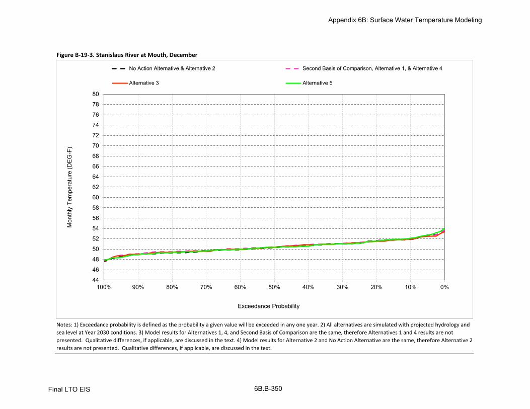
Figure B-19-3. Stanislaus River at Mouth, December
Notes: 1) Exceedance probability is defined as the probability a given value will be exceeded in any one year. 2) All alternatives are simulated with projected hydrology and
sea level at Year 2030 conditions. 3) Model results for Alternatives 1, 4, and Second Basis of Comparison are the same, therefore Alternatives 1 and 4 results are not
presented. Qualitative differences, if applicable, are discussed in the text. 4) Model results for Alternative 2 and No Action Alternative are the same, therefore Alternative 2
results are not presented. Qualitative differences, if applicable, are discussed in the text.
44
46
48
50
52
54
56
58
60
62
64
66
68
70
72
74
76
78
80
0%10%20%30%40%50%60%70%80%90%100%
Exceedance Probability
No Action Alternative & Alternative 2 Second Basis of Comparison, Alternative 1, & Alternative 4
Alternative 3 Alternative 5
Mon
thly
Tem
pera
ture
(DE
G-F
)
Appendix 6B: Surface Water Temperature Modeling
Final LTO EIS 6B.B-350

Figure B-19-4. Stanislaus River at Mouth, January
Notes: 1) Exceedance probability is defined as the probability a given value will be exceeded in any one year. 2) All alternatives are simulated with projected hydrology and
sea level at Year 2030 conditions. 3) Model results for Alternatives 1, 4, and Second Basis of Comparison are the same, therefore Alternatives 1 and 4 results are not
presented. Qualitative differences, if applicable, are discussed in the text. 4) Model results for Alternative 2 and No Action Alternative are the same, therefore Alternative 2
results are not presented. Qualitative differences, if applicable, are discussed in the text.
44
46
48
50
52
54
56
58
60
62
64
66
68
70
72
74
76
78
80
0%10%20%30%40%50%60%70%80%90%100%
Exceedance Probability
No Action Alternative & Alternative 2 Second Basis of Comparison, Alternative 1, & Alternative 4
Alternative 3 Alternative 5
Mon
thly
Tem
pera
ture
(DE
G-F
)
Appendix 6B: Surface Water Temperature Modeling
Final LTO EIS 6B.B-351

Figure B-19-5. Stanislaus River at Mouth, February
Notes: 1) Exceedance probability is defined as the probability a given value will be exceeded in any one year. 2) All alternatives are simulated with projected hydrology and
sea level at Year 2030 conditions. 3) Model results for Alternatives 1, 4, and Second Basis of Comparison are the same, therefore Alternatives 1 and 4 results are not
presented. Qualitative differences, if applicable, are discussed in the text. 4) Model results for Alternative 2 and No Action Alternative are the same, therefore Alternative 2
results are not presented. Qualitative differences, if applicable, are discussed in the text.
44
46
48
50
52
54
56
58
60
62
64
66
68
70
72
74
76
78
80
0%10%20%30%40%50%60%70%80%90%100%
Exceedance Probability
No Action Alternative & Alternative 2 Second Basis of Comparison, Alternative 1, & Alternative 4
Alternative 3 Alternative 5
Mon
thly
Tem
pera
ture
(DE
G-F
)
Appendix 6B: Surface Water Temperature Modeling
Final LTO EIS 6B.B-352

Figure B-19-6. Stanislaus River at Mouth, March
Notes: 1) Exceedance probability is defined as the probability a given value will be exceeded in any one year. 2) All alternatives are simulated with projected hydrology and
sea level at Year 2030 conditions. 3) Model results for Alternatives 1, 4, and Second Basis of Comparison are the same, therefore Alternatives 1 and 4 results are not
presented. Qualitative differences, if applicable, are discussed in the text. 4) Model results for Alternative 2 and No Action Alternative are the same, therefore Alternative 2
results are not presented. Qualitative differences, if applicable, are discussed in the text.
44
46
48
50
52
54
56
58
60
62
64
66
68
70
72
74
76
78
80
0%10%20%30%40%50%60%70%80%90%100%
Exceedance Probability
No Action Alternative & Alternative 2 Second Basis of Comparison, Alternative 1, & Alternative 4
Alternative 3 Alternative 5
Mon
thly
Tem
pera
ture
(DE
G-F
)
Appendix 6B: Surface Water Temperature Modeling
Final LTO EIS 6B.B-353

Figure B-19-7. Stanislaus River at Mouth, April
Notes: 1) Exceedance probability is defined as the probability a given value will be exceeded in any one year. 2) All alternatives are simulated with projected hydrology and
sea level at Year 2030 conditions. 3) Model results for Alternatives 1, 4, and Second Basis of Comparison are the same, therefore Alternatives 1 and 4 results are not
presented. Qualitative differences, if applicable, are discussed in the text. 4) Model results for Alternative 2 and No Action Alternative are the same, therefore Alternative 2
results are not presented. Qualitative differences, if applicable, are discussed in the text.
44
46
48
50
52
54
56
58
60
62
64
66
68
70
72
74
76
78
80
0%10%20%30%40%50%60%70%80%90%100%
Exceedance Probability
No Action Alternative & Alternative 2 Second Basis of Comparison, Alternative 1, & Alternative 4
Alternative 3 Alternative 5
Mon
thly
Tem
pera
ture
(DE
G-F
)
Appendix 6B: Surface Water Temperature Modeling
Final LTO EIS 6B.B-354

Figure B-19-8. Stanislaus River at Mouth, May
Notes: 1) Exceedance probability is defined as the probability a given value will be exceeded in any one year. 2) All alternatives are simulated with projected hydrology and
sea level at Year 2030 conditions. 3) Model results for Alternatives 1, 4, and Second Basis of Comparison are the same, therefore Alternatives 1 and 4 results are not
presented. Qualitative differences, if applicable, are discussed in the text. 4) Model results for Alternative 2 and No Action Alternative are the same, therefore Alternative 2
results are not presented. Qualitative differences, if applicable, are discussed in the text.
44
46
48
50
52
54
56
58
60
62
64
66
68
70
72
74
76
78
80
0%10%20%30%40%50%60%70%80%90%100%
Exceedance Probability
No Action Alternative & Alternative 2 Second Basis of Comparison, Alternative 1, & Alternative 4
Alternative 3 Alternative 5
Mon
thly
Tem
pera
ture
(DE
G-F
)
Appendix 6B: Surface Water Temperature Modeling
Final LTO EIS 6B.B-355

Figure B-19-9. Stanislaus River at Mouth, June
Notes: 1) Exceedance probability is defined as the probability a given value will be exceeded in any one year. 2) All alternatives are simulated with projected hydrology and
sea level at Year 2030 conditions. 3) Model results for Alternatives 1, 4, and Second Basis of Comparison are the same, therefore Alternatives 1 and 4 results are not
presented. Qualitative differences, if applicable, are discussed in the text. 4) Model results for Alternative 2 and No Action Alternative are the same, therefore Alternative 2
results are not presented. Qualitative differences, if applicable, are discussed in the text.
44
46
48
50
52
54
56
58
60
62
64
66
68
70
72
74
76
78
80
0%10%20%30%40%50%60%70%80%90%100%
Exceedance Probability
No Action Alternative & Alternative 2 Second Basis of Comparison, Alternative 1, & Alternative 4
Alternative 3 Alternative 5
Mon
thly
Tem
pera
ture
(DE
G-F
)
Appendix 6B: Surface Water Temperature Modeling
Final LTO EIS 6B.B-356

Figure B-19-10. Stanislaus River at Mouth, July
Notes: 1) Exceedance probability is defined as the probability a given value will be exceeded in any one year. 2) All alternatives are simulated with projected hydrology and
sea level at Year 2030 conditions. 3) Model results for Alternatives 1, 4, and Second Basis of Comparison are the same, therefore Alternatives 1 and 4 results are not
presented. Qualitative differences, if applicable, are discussed in the text. 4) Model results for Alternative 2 and No Action Alternative are the same, therefore Alternative 2
results are not presented. Qualitative differences, if applicable, are discussed in the text.
44
46
48
50
52
54
56
58
60
62
64
66
68
70
72
74
76
78
80
0%10%20%30%40%50%60%70%80%90%100%
Exceedance Probability
No Action Alternative & Alternative 2 Second Basis of Comparison, Alternative 1, & Alternative 4
Alternative 3 Alternative 5
Mon
thly
Tem
pera
ture
(DE
G-F
)
Appendix 6B: Surface Water Temperature Modeling
Final LTO EIS 6B.B-357

Figure B-19-11. Stanislaus River at Mouth, August
Notes: 1) Exceedance probability is defined as the probability a given value will be exceeded in any one year. 2) All alternatives are simulated with projected hydrology and
sea level at Year 2030 conditions. 3) Model results for Alternatives 1, 4, and Second Basis of Comparison are the same, therefore Alternatives 1 and 4 results are not
presented. Qualitative differences, if applicable, are discussed in the text. 4) Model results for Alternative 2 and No Action Alternative are the same, therefore Alternative 2
results are not presented. Qualitative differences, if applicable, are discussed in the text.
44
46
48
50
52
54
56
58
60
62
64
66
68
70
72
74
76
78
80
0%10%20%30%40%50%60%70%80%90%100%
Exceedance Probability
No Action Alternative & Alternative 2 Second Basis of Comparison, Alternative 1, & Alternative 4
Alternative 3 Alternative 5
Mon
thly
Tem
pera
ture
(DE
G-F
)
Appendix 6B: Surface Water Temperature Modeling
Final LTO EIS 6.BB-358

Figure B-19-12. Stanislaus River at Mouth, September
Notes: 1) Exceedance probability is defined as the probability a given value will be exceeded in any one year. 2) All alternatives are simulated with projected hydrology and
sea level at Year 2030 conditions. 3) Model results for Alternatives 1, 4, and Second Basis of Comparison are the same, therefore Alternatives 1 and 4 results are not
presented. Qualitative differences, if applicable, are discussed in the text. 4) Model results for Alternative 2 and No Action Alternative are the same, therefore Alternative 2
results are not presented. Qualitative differences, if applicable, are discussed in the text.
44
46
48
50
52
54
56
58
60
62
64
66
68
70
72
74
76
78
80
0%10%20%30%40%50%60%70%80%90%100%
Exceedance Probability
No Action Alternative & Alternative 2 Second Basis of Comparison, Alternative 1, & Alternative 4
Alternative 3 Alternative 5
Mon
thly
Tem
pera
ture
(DE
G-F
)
Appendix 6B: Surface Water Temperature Modeling
Final LTO EIS 6B.B-359

Oct Nov Dec Jan Feb Mar Apr May Jun Jul Aug Sep
10% 64 59 52 51 55 60 62 65 72 77 75 7220% 63 57 52 51 54 60 61 65 72 75 74 7130% 62 57 51 50 54 59 60 64 71 75 74 7040% 61 56 51 50 53 59 59 62 70 74 73 7050% 60 56 50 49 53 58 58 61 68 74 73 6960% 60 55 50 49 53 57 57 61 65 73 73 6970% 59 55 50 49 52 56 56 60 64 73 72 6980% 59 55 49 48 52 54 56 59 63 72 72 6890% 58 54 49 48 51 52 55 58 62 69 71 67
Full Simulation Periodb 61 56 50 50 53 57 58 62 67 73 73 69
Wet (32%) 57 53 49 49 52 54 55 59 63 70 70 67Above Normal (16%) 61 57 51 50 53 58 58 62 67 73 73 69Below Normal (13%) 60 55 50 49 53 58 59 61 69 74 73 70
Dry (24%) 61 56 50 49 53 59 60 63 70 75 73 70Critical (15%) 64 58 51 50 54 60 62 66 71 76 75 72
Oct Nov Dec Jan Feb Mar Apr May Jun Jul Aug Sep
10% 67 58 52 51 55 60 64 64 72 76 75 7120% 65 58 52 51 54 59 63 63 71 75 74 7130% 64 57 51 50 54 59 62 63 70 75 74 7040% 64 56 51 50 53 58 61 61 70 74 73 7050% 63 56 50 49 52 57 60 61 67 74 73 6960% 62 55 50 49 52 57 58 61 65 73 73 6970% 62 55 50 49 52 56 57 60 62 73 72 6880% 61 55 49 48 51 55 56 59 61 71 72 6890% 61 54 49 48 50 54 55 58 59 70 71 67
Full Simulation Periodb 63 56 51 50 53 57 60 61 66 73 73 69
Wet (32%) 59 53 49 49 52 55 56 59 61 70 71 66Above Normal (16%) 64 57 51 50 53 58 59 61 66 73 73 69Below Normal (13%) 62 55 50 49 52 58 60 61 68 74 73 69
Dry (24%) 63 56 50 49 53 58 62 63 70 75 73 70Critical (15%) 66 58 51 50 54 60 64 64 71 76 75 72
Oct Nov Dec Jan Feb Mar Apr May Jun Jul Aug Sep
0.1 2.2 -0.2 0.1 -0.1 -0.5 -0.2 1.6 -1.4 -0.2 -0.3 -0.1 -0.4
0.2 2.3 0.3 0.1 0.0 -0.2 -0.2 1.9 -1.1 -0.2 -0.1 -0.1 -0.1
0.3 2.6 0.1 0.1 0.0 -0.2 -0.4 1.9 -0.9 -0.3 -0.1 0.0 -0.2
0.4 3.2 -0.2 0.1 0.0 -0.2 -0.5 2.0 -0.7 -0.6 -0.1 0.0 -0.2
0.5 2.8 0.2 0.2 -0.1 -0.4 -0.6 2.1 0.2 -0.6 -0.2 0.0 -0.1
0.6 2.6 0.1 0.2 0.0 -0.4 -0.3 1.1 0.1 -0.2 -0.1 0.0 -0.2
0.7 2.7 0.1 0.0 0.0 -0.2 0.6 0.6 0.0 -1.5 -0.2 0.0 -0.2
0.8 2.6 0.0 0.2 0.0 -0.1 1.9 0.4 0.4 -1.6 -0.2 0.1 0.00.9 2.5 0.0 0.1 0.1 -0.2 2.1 0.5 0.5 -2.6 1.1 0.6 0.2
Full Simulation Periodb 2.4 0.1 0.1 0.0 -0.2 0.2 1.3 -0.4 -1.0 -0.1 0.1 -0.1
Wet (32%) 2.2 -0.1 0.0 -0.1 -0.2 1.1 0.4 0.4 -2.4 0.0 0.5 -0.1
Above Normal (16%) 2.6 0.0 0.1 -0.1 -0.3 0.0 1.3 -0.5 -0.6 -0.1 0.0 -0.1
Below Normal (13%) 2.2 -0.2 0.1 -0.1 -0.4 -0.4 1.9 -0.2 -0.7 -0.2 0.0 -0.2
Dry (24%) 2.7 0.2 0.2 0.0 -0.3 -0.4 2.0 -0.8 -0.2 0.0 0.0 -0.1
Critical (15%) 1.8 0.4 0.3 0.1 0.0 0.0 1.5 -1.2 -0.3 -0.2 -0.1 -0.1
a Exceedance probability is defined as the probability a given value will be exceeded in any one year.
b Based on an 81-year simulation period.
Probability of Exceedancea
Long Term
Water Year Typesc
c As defined by the Sacramento Valley 40-30-30 Index Water Year Hydrologic Classification (SWRCB D-1641, 1999); projected to Year 2030.
Notes: 1) All alternatives are simulated with projected hydrology and sea level at Year 2030 conditions. 2) Model results for Alternatives 1, 4, and Second Basis of Comparison are the same,
therefore Second Basis of Comparison and Alternative 4 results are not presented. Qualitative differences, if applicable, are discussed in the text. 3) Model results for Alternative 2 and No Action
Alternative are the same, therefore Alternative 2 results are not presented. Qualitative differences, if applicable, are discussed in the text.
Probability of Exceedancea
Long Term
Water Year Typesc
Alternative 1 minus No Action Alternative
Statistic
Monthly Temperature (DEG-F)
Long Term
Water Year Typesc
Alternative 1
Statistic
Monthly Temperature (DEG-F)
No Action Alternative
Statistic
Monthly Temperature (DEG-F)
Probability of Exceedancea
Table B-19-1. Stanislaus River at Mouth, Monthly Temperature
Appendix 6B: Surface Water Temperature Modeling
Final LTO EIS 6B.B-360

Oct Nov Dec Jan Feb Mar Apr May Jun Jul Aug Sep
10% 64 59 52 51 55 60 62 65 72 77 75 7220% 63 57 52 51 54 60 61 65 72 75 74 7130% 62 57 51 50 54 59 60 64 71 75 74 7040% 61 56 51 50 53 59 59 62 70 74 73 7050% 60 56 50 49 53 58 58 61 68 74 73 6960% 60 55 50 49 53 57 57 61 65 73 73 6970% 59 55 50 49 52 56 56 60 64 73 72 6980% 59 55 49 48 52 54 56 59 63 72 72 6890% 58 54 49 48 51 52 55 58 62 69 71 67
Full Simulation Periodb 61 56 50 50 53 57 58 62 67 73 73 69
Wet (32%) 57 53 49 49 52 54 55 59 63 70 70 67Above Normal (16%) 61 57 51 50 53 58 58 62 67 73 73 69Below Normal (13%) 60 55 50 49 53 58 59 61 69 74 73 70
Dry (24%) 61 56 50 49 53 59 60 63 70 75 73 70Critical (15%) 64 58 51 50 54 60 62 66 71 76 75 72
Oct Nov Dec Jan Feb Mar Apr May Jun Jul Aug Sep
10% 66 58 52 52 55 61 63 66 73 77 75 7220% 65 58 52 51 55 60 62 65 72 76 74 7130% 64 57 51 50 54 59 60 64 72 75 74 7040% 63 56 51 50 53 59 60 63 72 75 73 7050% 63 56 50 49 53 58 58 62 71 75 73 6960% 62 55 50 49 52 57 57 62 70 74 73 6970% 62 55 50 49 52 57 57 61 69 74 72 6980% 61 55 49 49 51 55 56 60 68 74 72 6890% 61 54 49 48 50 54 55 59 67 73 71 62
Full Simulation Periodb 63 56 50 50 53 58 59 62 70 74 72 69
Wet (32%) 59 53 49 49 51 55 56 60 67 71 70 66Above Normal (16%) 64 57 51 50 53 58 58 62 71 75 73 69Below Normal (13%) 62 55 50 49 52 58 59 62 71 75 73 69
Dry (24%) 63 56 50 49 54 59 60 64 72 75 73 70Critical (15%) 65 58 51 50 55 60 62 66 72 76 75 71
Oct Nov Dec Jan Feb Mar Apr May Jun Jul Aug Sep
0.1 1.4 -0.3 0.1 0.2 0.2 0.4 0.6 0.3 0.9 0.4 0.1 -0.1
0.2 2.2 0.2 -0.1 0.0 0.4 0.0 0.4 0.0 0.7 0.5 -0.1 -0.1
0.3 2.3 -0.1 0.0 0.0 0.0 0.1 0.2 0.1 1.3 0.6 0.0 -0.2
0.4 2.6 -0.2 0.1 0.0 0.0 0.1 1.0 0.8 1.5 0.7 -0.1 0.10.5 2.7 -0.1 0.1 0.0 -0.1 0.3 0.4 1.5 3.3 0.9 0.1 0.0
0.6 2.8 0.1 0.1 0.0 -0.3 0.3 0.2 1.0 5.0 1.1 0.0 0.0
0.7 2.7 0.0 0.0 0.0 -0.2 1.1 0.4 1.1 5.4 0.9 0.0 0.00.8 2.6 0.1 0.1 0.1 -0.5 1.4 0.4 1.5 5.8 1.8 0.1 -0.1
0.9 2.4 0.0 0.0 0.0 -0.3 1.5 0.6 1.1 5.7 3.6 0.7 -4.7
Full Simulation Periodb 2.2 0.0 0.0 0.0 -0.1 0.5 0.4 0.8 2.6 0.6 -0.2 -0.4
Wet (32%) 2.0 0.0 0.0 0.0 -0.3 1.3 0.3 1.2 3.8 0.4 -0.6 -0.8
Above Normal (16%) 2.6 0.0 0.0 0.0 -0.3 -0.2 0.4 0.8 4.2 1.7 0.2 0.1Below Normal (13%) 2.1 -0.1 0.0 0.0 -0.4 0.3 0.7 1.0 2.1 0.6 0.0 0.0
Dry (24%) 2.6 0.1 0.1 0.0 0.3 0.1 0.4 0.6 1.3 0.4 -0.1 -0.2
Critical (15%) 1.2 0.0 0.1 0.0 0.5 0.3 0.3 0.2 0.9 0.3 -0.2 -0.6
a Exceedance probability is defined as the probability a given value will be exceeded in any one year.
b Based on an 81-year simulation period.
Probability of Exceedancea
Long Term
Water Year Typesc
c As defined by the Sacramento Valley 40-30-30 Index Water Year Hydrologic Classification (SWRCB D-1641, 1999); projected to Year 2030.
Notes: 1) All alternatives are simulated with projected hydrology and sea level at Year 2030 conditions. 2) Model results for Alternatives 1, 4, and Second Basis of Comparison are the same,
therefore Alternative 1 and 4 results are not presented. Qualitative differences, if applicable, are discussed in the text. 3) Model results for Alternative 2 and No Action Alternative are the same,
therefore Alternative 2 results are not presented. Qualitative differences, if applicable, are discussed in the text.
Probability of Exceedancea
Long Term
Water Year Typesc
Alternative 3 minus No Action Alternative
Statistic
Monthly Temperature (DEG-F)
Long Term
Water Year Typesc
Alternative 3
Statistic
Monthly Temperature (DEG-F)
No Action Alternative
Statistic
Monthly Temperature (DEG-F)
Probability of Exceedancea
Table B-19-2. Stanislaus River at Mouth, Monthly Temperature
Appendix 6B: Surface Water Temperature Modeling
Final LTO EIS 6B.B-361
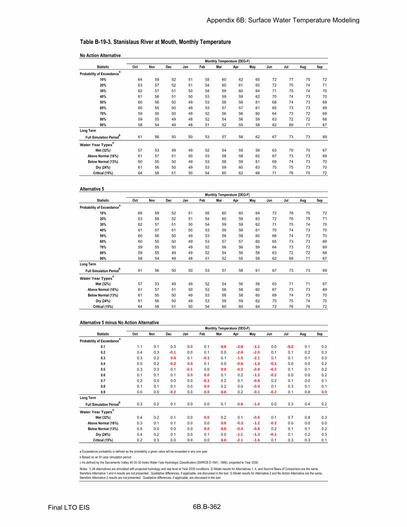
Oct Nov Dec Jan Feb Mar Apr May Jun Jul Aug Sep
10% 64 59 52 51 55 60 62 65 72 77 75 7220% 63 57 52 51 54 60 61 65 72 75 74 7130% 62 57 51 50 54 59 60 64 71 75 74 7040% 61 56 51 50 53 59 59 62 70 74 73 7050% 60 56 50 49 53 58 58 61 68 74 73 6960% 60 55 50 49 53 57 57 61 65 73 73 6970% 59 55 50 49 52 56 56 60 64 73 72 6980% 59 55 49 48 52 54 56 59 63 72 72 6890% 58 54 49 48 51 52 55 58 62 69 71 67
Full Simulation Periodb 61 56 50 50 53 57 58 62 67 73 73 69
Wet (32%) 57 53 49 49 52 54 55 59 63 70 70 67Above Normal (16%) 61 57 51 50 53 58 58 62 67 73 73 69Below Normal (13%) 60 55 50 49 53 58 59 61 69 74 73 70
Dry (24%) 61 56 50 49 53 59 60 63 70 75 73 70Critical (15%) 64 58 51 50 54 60 62 66 71 76 75 72
Oct Nov Dec Jan Feb Mar Apr May Jun Jul Aug Sep
10% 65 59 52 51 55 60 60 64 72 76 75 7220% 63 58 52 51 54 60 59 63 72 76 75 7130% 62 57 51 50 54 59 59 62 71 75 74 7040% 61 57 51 50 53 59 58 61 70 74 73 7050% 60 56 50 49 53 58 58 60 68 74 73 7060% 60 55 50 49 53 57 57 60 65 73 73 6970% 59 55 50 49 52 56 56 59 64 73 72 6980% 59 55 49 49 52 54 56 58 63 72 72 6890% 58 54 49 48 51 52 55 58 62 69 71 67
Full Simulation Periodb 61 56 50 50 53 57 58 61 67 73 73 69
Wet (32%) 57 53 49 49 52 54 56 58 63 71 71 67Above Normal (16%) 61 57 51 50 53 58 58 60 67 73 73 69Below Normal (13%) 61 55 50 49 53 58 58 60 69 74 73 70
Dry (24%) 61 56 50 49 53 59 59 62 70 75 74 70Critical (15%) 64 58 51 50 54 60 60 64 72 76 76 72
Oct Nov Dec Jan Feb Mar Apr May Jun Jul Aug Sep
0.1 1.1 0.1 0.3 0.0 0.1 0.0 -2.0 -1.1 0.0 -0.2 0.1 0.20.2 0.4 0.3 -0.1 0.0 0.1 0.0 -2.0 -2.0 0.1 0.1 0.2 0.30.3 0.3 0.2 0.0 0.1 -0.1 0.1 -1.5 -2.1 0.1 0.1 0.1 0.00.4 0.5 0.2 -0.2 0.0 0.1 0.0 -0.5 -1.3 -0.1 0.0 0.0 0.20.5 0.3 0.3 0.1 -0.1 0.0 0.0 -0.2 -0.9 -0.2 0.1 0.1 0.20.6 0.1 0.1 0.1 0.0 0.0 0.1 0.2 -1.2 -0.2 0.0 0.0 0.20.7 0.2 0.0 0.0 0.0 -0.1 0.2 0.1 -0.8 0.2 0.1 0.0 0.10.8 0.1 0.1 0.1 0.0 0.0 0.2 0.0 -0.4 0.1 0.3 0.1 0.10.9 0.0 0.0 -0.2 0.0 0.0 0.0 0.2 -0.1 -0.2 0.1 0.6 0.0
Full Simulation Periodb 0.3 0.2 0.1 0.0 0.0 0.1 -0.6 -1.0 0.0 0.3 0.4 0.2
Wet (32%) 0.4 0.2 0.1 0.0 0.0 0.2 0.1 -0.5 0.1 0.7 0.8 0.3Above Normal (16%) 0.3 0.1 0.1 0.0 0.0 0.0 -0.3 -1.2 -0.2 0.0 0.0 0.0Below Normal (13%) 0.5 0.0 0.0 0.0 0.0 0.0 -0.4 -0.8 0.2 0.1 0.1 0.2
Dry (24%) 0.4 0.2 0.1 0.0 0.1 0.0 -1.1 -1.3 -0.1 0.1 0.2 0.3Critical (15%) 0.2 0.3 0.0 0.0 0.0 0.0 -2.1 -1.6 0.1 0.3 0.3 0.1
a Exceedance probability is defined as the probability a given value will be exceeded in any one year.
b Based on an 81-year simulation period.
Probability of Exceedancea
Long Term
Water Year Typesc
c As defined by the Sacramento Valley 40-30-30 Index Water Year Hydrologic Classification (SWRCB D-1641, 1999); projected to Year 2030.
Notes: 1) All alternatives are simulated with projected hydrology and sea level at Year 2030 conditions. 2) Model results for Alternatives 1, 4, and Second Basis of Comparison are the same,
therefore Alternative 1 and 4 results are not presented. Qualitative differences, if applicable, are discussed in the text. 3) Model results for Alternative 2 and No Action Alternative are the same,
therefore Alternative 2 results are not presented. Qualitative differences, if applicable, are discussed in the text.
Probability of Exceedancea
Long Term
Water Year Typesc
Alternative 5 minus No Action Alternative
Statistic
Monthly Temperature (DEG-F)
Long Term
Water Year Typesc
Alternative 5
Statistic
Monthly Temperature (DEG-F)
No Action Alternative
Statistic
Monthly Temperature (DEG-F)
Probability of Exceedancea
Table B-19-3. Stanislaus River at Mouth, Monthly Temperature
Appendix 6B: Surface Water Temperature Modeling
Final LTO EIS 6B.B-362

Oct Nov Dec Jan Feb Mar Apr May Jun Jul Aug Sep
10% 67 58 52 51 55 60 64 64 72 76 75 7120% 65 58 52 51 54 59 63 63 71 75 74 7130% 64 57 51 50 54 59 62 63 70 75 74 7040% 64 56 51 50 53 58 61 61 70 74 73 7050% 63 56 50 49 52 57 60 61 67 74 73 6960% 62 55 50 49 52 57 58 61 65 73 73 6970% 62 55 50 49 52 56 57 60 62 73 72 6880% 61 55 49 48 51 55 56 59 61 71 72 6890% 61 54 49 48 50 54 55 58 59 70 71 67
Full Simulation Periodb 63 56 51 50 53 57 60 61 66 73 73 69
Wet (32%) 59 53 49 49 52 55 56 59 61 70 71 66Above Normal (16%) 64 57 51 50 53 58 59 61 66 73 73 69Below Normal (13%) 62 55 50 49 52 58 60 61 68 74 73 69
Dry (24%) 63 56 50 49 53 58 62 63 70 75 73 70Critical (15%) 66 58 51 50 54 60 64 64 71 76 75 72
Oct Nov Dec Jan Feb Mar Apr May Jun Jul Aug Sep
10% 64 59 52 51 55 60 62 65 72 77 75 7220% 63 57 52 51 54 60 61 65 72 75 74 7130% 62 57 51 50 54 59 60 64 71 75 74 7040% 61 56 51 50 53 59 59 62 70 74 73 7050% 60 56 50 49 53 58 58 61 68 74 73 6960% 60 55 50 49 53 57 57 61 65 73 73 6970% 59 55 50 49 52 56 56 60 64 73 72 6980% 59 55 49 48 52 54 56 59 63 72 72 6890% 58 54 49 48 51 52 55 58 62 69 71 67
Full Simulation Periodb 61 56 50 50 53 57 58 62 67 73 73 69
Wet (32%) 57 53 49 49 52 54 55 59 63 70 70 67Above Normal (16%) 61 57 51 50 53 58 58 62 67 73 73 69Below Normal (13%) 60 55 50 49 53 58 59 61 69 74 73 70
Dry (24%) 61 56 50 49 53 59 60 63 70 75 73 70Critical (15%) 64 58 51 50 54 60 62 66 71 76 75 72
Oct Nov Dec Jan Feb Mar Apr May Jun Jul Aug Sep
0.1 -2.2 0.2 -0.1 0.1 0.5 0.2 -1.6 1.4 0.2 0.3 0.1 0.40.2 -2.3 -0.3 -0.1 0.0 0.2 0.2 -1.9 1.1 0.2 0.1 0.1 0.10.3 -2.6 -0.1 -0.1 0.0 0.2 0.4 -1.9 0.9 0.3 0.1 0.0 0.20.4 -3.2 0.2 -0.1 0.0 0.2 0.5 -2.0 0.7 0.6 0.1 0.0 0.20.5 -2.8 -0.2 -0.2 0.1 0.4 0.6 -2.1 -0.2 0.6 0.2 0.0 0.10.6 -2.6 -0.1 -0.2 0.0 0.4 0.3 -1.1 -0.1 0.2 0.1 0.0 0.20.7 -2.7 -0.1 0.0 0.0 0.2 -0.6 -0.6 0.0 1.5 0.2 0.0 0.20.8 -2.6 0.0 -0.2 0.0 0.1 -1.9 -0.4 -0.4 1.6 0.2 -0.1 0.0
0.9 -2.5 0.0 -0.1 -0.1 0.2 -2.1 -0.5 -0.5 2.6 -1.1 -0.6 -0.2
Full Simulation Periodb
-2.4 -0.1 -0.1 0.0 0.2 -0.2 -1.3 0.4 1.0 0.1 -0.1 0.1
Wet (32%) -2.2 0.1 0.0 0.1 0.2 -1.1 -0.4 -0.4 2.4 0.0 -0.5 0.1Above Normal (16%) -2.6 0.0 -0.1 0.1 0.3 0.0 -1.3 0.5 0.6 0.1 0.0 0.1Below Normal (13%) -2.2 0.2 -0.1 0.1 0.4 0.4 -1.9 0.2 0.7 0.2 0.0 0.2
Dry (24%) -2.7 -0.2 -0.2 0.0 0.3 0.4 -2.0 0.8 0.2 0.0 0.0 0.1Critical (15%) -1.8 -0.4 -0.3 -0.1 0.0 0.0 -1.5 1.2 0.3 0.2 0.1 0.1
a Exceedance probability is defined as the probability a given value will be exceeded in any one year.
b Based on an 81-year simulation period.
Probability of Exceedancea
Long Term
Water Year Typesc
c As defined by the Sacramento Valley 40-30-30 Index Water Year Hydrologic Classification (SWRCB D-1641, 1999); projected to Year 2030.
Notes: 1) All alternatives are simulated with projected hydrology and sea level at Year 2030 conditions. 2) Model results for Alternatives 1, 4, and Second Basis of Comparison are the same,
therefore Alternative 1 and 4 results are not presented. Qualitative differences, if applicable, are discussed in the text. 3) Model results for Alternative 2 and No Action Alternative are the same,
Probability of Exceedancea
Long Term
Water Year Typesc
No Action Alternative minus Second Basis of Comparison
Statistic
Monthly Temperature (DEG-F)
Long Term
Water Year Typesc
No Action Alternative
Statistic
Monthly Temperature (DEG-F)
Second Basis of Comparison
Statistic
Monthly Temperature (DEG-F)
Probability of Exceedancea
therefore Alternative 2 results are not presented. Qualitative differences, if applicable, are discussed in the text.
Table B-19-4. Stanislaus River at Mouth, Monthly Temperature
Appendix 6B: Surface Water Temperature Modeling
Final LTO EIS 6B.B-362

Oct Nov Dec Jan Feb Mar Apr May Jun Jul Aug Sep
10% 67 58 52 51 55 60 64 64 72 76 75 7120% 65 58 52 51 54 59 63 63 71 75 74 7130% 64 57 51 50 54 59 62 63 70 75 74 7040% 64 56 51 50 53 58 61 61 70 74 73 7050% 63 56 50 49 52 57 60 61 67 74 73 6960% 62 55 50 49 52 57 58 61 65 73 73 6970% 62 55 50 49 52 56 57 60 62 73 72 6880% 61 55 49 48 51 55 56 59 61 71 72 6890% 61 54 49 48 50 54 55 58 59 70 71 67
Full Simulation Periodb 63 56 51 50 53 57 60 61 66 73 73 69
Wet (32%) 59 53 49 49 52 55 56 59 61 70 71 66Above Normal (16%) 64 57 51 50 53 58 59 61 66 73 73 69Below Normal (13%) 62 55 50 49 52 58 60 61 68 74 73 69
Dry (24%) 63 56 50 49 53 58 62 63 70 75 73 70Critical (15%) 66 58 51 50 54 60 64 64 71 76 75 72
Oct Nov Dec Jan Feb Mar Apr May Jun Jul Aug Sep
10% 66 58 52 52 55 61 63 66 73 77 75 7220% 65 58 52 51 55 60 62 65 72 76 74 7130% 64 57 51 50 54 59 60 64 72 75 74 7040% 63 56 51 50 53 59 60 63 72 75 73 7050% 63 56 50 49 53 58 58 62 71 75 73 6960% 62 55 50 49 52 57 57 62 70 74 73 6970% 62 55 50 49 52 57 57 61 69 74 72 6980% 61 55 49 49 51 55 56 60 68 74 72 6890% 61 54 49 48 50 54 55 59 67 73 71 62
Full Simulation Periodb 63 56 50 50 53 58 59 62 70 74 72 69
Wet (32%) 59 53 49 49 51 55 56 60 67 71 70 66Above Normal (16%) 64 57 51 50 53 58 58 62 71 75 73 69Below Normal (13%) 62 55 50 49 52 58 59 62 71 75 73 69
Dry (24%) 63 56 50 49 54 59 60 64 72 75 73 70Critical (15%) 65 58 51 50 55 60 62 66 72 76 75 71
Oct Nov Dec Jan Feb Mar Apr May Jun Jul Aug Sep
0.1 -0.8 -0.1 0.0 0.3 0.7 0.5 -1.0 1.7 1.1 0.7 0.2 0.30.2 -0.1 -0.1 -0.1 0.0 0.6 0.2 -1.5 1.1 0.9 0.6 0.0 0.10.3 -0.3 -0.2 -0.1 0.0 0.3 0.5 -1.7 1.0 1.6 0.7 0.0 0.0
0.4 -0.6 0.0 0.0 0.0 0.2 0.5 -1.1 1.5 2.1 0.8 0.0 0.30.5 0.0 -0.2 -0.1 0.1 0.3 0.9 -1.7 1.3 3.9 1.1 0.1 0.00.6 0.1 0.0 -0.1 -0.1 0.1 0.7 -1.0 0.9 5.2 1.2 -0.1 0.20.7 0.0 -0.1 -0.1 0.0 0.0 0.4 -0.2 1.1 7.0 1.1 0.0 0.20.8 0.1 0.1 -0.1 0.1 -0.4 -0.4 0.0 1.1 7.5 2.0 0.0 -0.1
0.9 -0.2 0.1 -0.1 0.0 -0.1 -0.6 0.1 0.6 8.3 2.6 0.1 -4.8
Full Simulation Periodb
-0.2 -0.1 -0.1 0.0 0.1 0.3 -0.9 1.2 3.6 0.7 -0.3 -0.2
Wet (32%) -0.2 0.0 0.0 0.1 -0.1 0.2 -0.1 0.8 6.1 0.4 -1.1 -0.6
Above Normal (16%) 0.0 0.0 -0.1 0.1 0.0 -0.1 -0.9 1.2 4.9 1.8 0.2 0.2Below Normal (13%) -0.2 0.0 -0.2 0.0 0.0 0.6 -1.2 1.2 2.8 0.7 0.0 0.2
Dry (24%) -0.2 0.0 0.0 0.0 0.5 0.5 -1.6 1.4 1.5 0.4 0.0 -0.1
Critical (15%) -0.6 -0.4 -0.2 -0.1 0.5 0.3 -1.2 1.4 1.2 0.5 -0.1 -0.5
a Exceedance probability is defined as the probability a given value will be exceeded in any one year.
b Based on an 81-year simulation period.
Probability of Exceedancea
Long Term
Water Year Typesc
c As defined by the Sacramento Valley 40-30-30 Index Water Year Hydrologic Classification (SWRCB D-1641, 1999); projected to Year 2030.
Notes: 1) All alternatives are simulated with projected hydrology and sea level at Year 2030 conditions. 2) Model results for Alternatives 1, 4, and Second Basis of Comparison are the same,
therefore Alternative 1 and 4 results are not presented. Qualitative differences, if applicable, are discussed in the text. 3) Model results for Alternative 2 and No Action Alternative are the same,
therefore Alternative 2 results are not presented. Qualitative differences, if applicable, are discussed in the text.
Probability of Exceedancea
Long Term
Water Year Typesc
Alternative 3 minus Second Basis of Comparison
Statistic
Monthly Temperature (DEG-F)
Long Term
Water Year Typesc
Alternative 3
Statistic
Monthly Temperature (DEG-F)
Second Basis of Comparison
Statistic
Monthly Temperature (DEG-F)
Probability of Exceedancea
Table B-19-5. Stanislaus River at Mouth, Monthly Temperature
Appendix 6B: Surface Water Temperature Modeling
Final LTO EIS 6B.B-363

Oct Nov Dec Jan Feb Mar Apr May Jun Jul Aug Sep
10% 67 58 52 51 55 60 64 64 72 76 75 7120% 65 58 52 51 54 59 63 63 71 75 74 7130% 64 57 51 50 54 59 62 63 70 75 74 7040% 64 56 51 50 53 58 61 61 70 74 73 7050% 63 56 50 49 52 57 60 61 67 74 73 6960% 62 55 50 49 52 57 58 61 65 73 73 6970% 62 55 50 49 52 56 57 60 62 73 72 6880% 61 55 49 48 51 55 56 59 61 71 72 6890% 61 54 49 48 50 54 55 58 59 70 71 67
Full Simulation Periodb 63 56 51 50 53 57 60 61 66 73 73 69
Wet (32%) 59 53 49 49 52 55 56 59 61 70 71 66Above Normal (16%) 64 57 51 50 53 58 59 61 66 73 73 69Below Normal (13%) 62 55 50 49 52 58 60 61 68 74 73 69
Dry (24%) 63 56 50 49 53 58 62 63 70 75 73 70Critical (15%) 66 58 51 50 54 60 64 64 71 76 75 72
Oct Nov Dec Jan Feb Mar Apr May Jun Jul Aug Sep
10% 65 59 52 51 55 60 60 64 72 76 75 7220% 63 58 52 51 54 60 59 63 72 76 75 7130% 62 57 51 50 54 59 59 62 71 75 74 7040% 61 57 51 50 53 59 58 61 70 74 73 7050% 60 56 50 49 53 58 58 60 68 74 73 7060% 60 55 50 49 53 57 57 60 65 73 73 6970% 59 55 50 49 52 56 56 59 64 73 72 6980% 59 55 49 49 52 54 56 58 63 72 72 6890% 58 54 49 48 51 52 55 58 62 69 71 67
Full Simulation Periodb 61 56 50 50 53 57 58 61 67 73 73 69
Wet (32%) 57 53 49 49 52 54 56 58 63 71 71 67Above Normal (16%) 61 57 51 50 53 58 58 60 67 73 73 69Below Normal (13%) 61 55 50 49 53 58 58 60 69 74 73 70
Dry (24%) 61 56 50 49 53 59 59 62 70 75 74 70Critical (15%) 64 58 51 50 54 60 60 64 72 76 76 72
Oct Nov Dec Jan Feb Mar Apr May Jun Jul Aug Sep
0.1 -1.1 0.3 0.2 0.1 0.6 0.2 -3.5 0.3 0.3 0.1 0.3 0.60.2 -1.9 0.0 -0.1 0.0 0.3 0.2 -3.9 -0.9 0.4 0.2 0.3 0.40.3 -2.3 0.1 -0.1 0.1 0.1 0.5 -3.4 -1.1 0.4 0.3 0.1 0.20.4 -2.8 0.4 -0.4 0.0 0.2 0.5 -2.5 -0.7 0.5 0.1 0.1 0.30.5 -2.5 0.1 -0.1 0.0 0.4 0.6 -2.3 -1.1 0.4 0.3 0.1 0.30.6 -2.5 0.1 -0.1 0.0 0.4 0.5 -0.9 -1.3 0.0 0.1 0.0 0.40.7 -2.6 0.0 0.0 0.1 0.1 -0.4 -0.5 -0.8 1.7 0.2 0.0 0.30.8 -2.5 0.2 -0.2 0.1 0.1 -1.7 -0.4 -0.8 1.7 0.5 0.0 0.00.9 -2.5 0.0 -0.2 0.0 0.2 -2.1 -0.3 -0.6 2.4 -1.0 0.0 -0.2
Full Simulation Periodb
-2.0 0.1 -0.1 0.0 0.3 -0.1 -1.9 -0.6 1.1 0.4 0.2 0.3
Wet (32%) -1.8 0.2 0.0 0.1 0.2 -0.9 -0.3 -0.8 2.5 0.7 0.3 0.4Above Normal (16%) -2.3 0.1 -0.1 0.1 0.3 0.0 -1.6 -0.8 0.5 0.1 0.0 0.2Below Normal (13%) -1.8 0.2 -0.1 0.1 0.4 0.4 -2.3 -0.6 0.9 0.3 0.1 0.3
Dry (24%) -2.4 0.1 -0.1 0.0 0.4 0.5 -3.1 -0.5 0.1 0.1 0.2 0.4Critical (15%) -1.6 0.0 -0.3 -0.1 0.0 0.0 -3.5 -0.3 0.4 0.5 0.4 0.2
a Exceedance probability is defined as the probability a given value will be exceeded in any one year.
b Based on an 81-year simulation period.
Probability of Exceedancea
Long Term
Water Year Typesc
c As defined by the Sacramento Valley 40-30-30 Index Water Year Hydrologic Classification (SWRCB D-1641, 1999); projected to Year 2030.
Notes: 1) All alternatives are simulated with projected hydrology and sea level at Year 2030 conditions. 2) Model results for Alternatives 1, 4, and Second Basis of Comparison are the same,
therefore Alternative 1 and 4 results are not presented. Qualitative differences, if applicable, are discussed in the text. 3) Model results for Alternative 2 and No Action Alternative are the same,
therefore Alternative 2 results are not presented. Qualitative differences, if applicable, are discussed in the text.
Probability of Exceedancea
Long Term
Water Year Typesc
Alternative 5 minus Second Basis of Comparison
Statistic
Monthly Temperature (DEG-F)
Long Term
Water Year Typesc
Alternative 5
Statistic
Monthly Temperature (DEG-F)
Second Basis of Comparison
Statistic
Monthly Temperature (DEG-F)
Probability of Exceedancea
Table B-19-6. Stanislaus River at Mouth, Monthly Temperature
Appendix 6B: Surface Water Temperature Modeling
Final LTO EIS 6B.B-364

B.20. Feather River Low Flow Channel
Appendix 6B: Surface Water Temperature Modeling
Final LTO EIS 6B.B-365

Figure B-20-1. Feather River Low Flow Channel, October
Notes: 1) Exceedance probability is defined as the probability a given value will be exceeded in any one year. 2) All alternatives are simulated with projected hydrology and
sea level at Year 2030 conditions. 3) Model results for Alternatives 1, 4, and Second Basis of Comparison are the same, therefore Alternatives 1 and 4 results are not
presented. Qualitative differences, if applicable, are discussed in the text. 4) Model results for Alternative 2 and No Action Alternative are the same, therefore Alternative 2
results are not presented. Qualitative differences, if applicable, are discussed in the text.
44
46
48
50
52
54
56
58
60
62
64
66
68
70
0%10%20%30%40%50%60%70%80%90%100%
Exceedance Probability
No Action Alternative & Alternative 2 Second Basis of Comparison, Alternative 1, & Alternative 4
Alternative 3 Alternative 5
Mon
thly
Tem
pera
ture
(DE
G-F
)
Appendix 6B: Surface Water Temperature Modeling
Final LTO EIS 6B.B-366
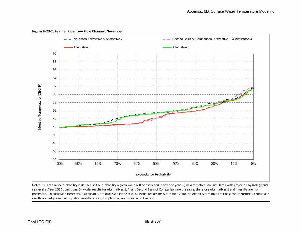
Figure B-20-2. Feather River Low Flow Channel, November
Notes: 1) Exceedance probability is defined as the probability a given value will be exceeded in any one year. 2) All alternatives are simulated with projected hydrology and
sea level at Year 2030 conditions. 3) Model results for Alternatives 1, 4, and Second Basis of Comparison are the same, therefore Alternatives 1 and 4 results are not
presented. Qualitative differences, if applicable, are discussed in the text. 4) Model results for Alternative 2 and No Action Alternative are the same, therefore Alternative 2
results are not presented. Qualitative differences, if applicable, are discussed in the text.
44
46
48
50
52
54
56
58
60
62
64
66
68
70
0%10%20%30%40%50%60%70%80%90%100%
Exceedance Probability
No Action Alternative & Alternative 2 Second Basis of Comparison, Alternative 1, & Alternative 4
Alternative 3 Alternative 5
Mon
thly
Tem
pera
ture
(DE
G-F
)
Appendix 6B: Surface Water Temperature Modeling
Final LTO EIS 6B.B-367

Figure B-20-3. Feather River Low Flow Channel, December
Notes: 1) Exceedance probability is defined as the probability a given value will be exceeded in any one year. 2) All alternatives are simulated with projected hydrology and
sea level at Year 2030 conditions. 3) Model results for Alternatives 1, 4, and Second Basis of Comparison are the same, therefore Alternatives 1 and 4 results are not
presented. Qualitative differences, if applicable, are discussed in the text. 4) Model results for Alternative 2 and No Action Alternative are the same, therefore Alternative 2
results are not presented. Qualitative differences, if applicable, are discussed in the text.
44
46
48
50
52
54
56
58
60
62
64
66
68
70
0%10%20%30%40%50%60%70%80%90%100%
Exceedance Probability
No Action Alternative & Alternative 2 Second Basis of Comparison, Alternative 1, & Alternative 4
Alternative 3 Alternative 5
Mon
thly
Tem
pera
ture
(DE
G-F
)
Appendix 6B: Surface Water Temperature Modeling
Final LTO EIS 6B.B-368

Figure B-20-4. Feather River Low Flow Channel, January
Notes: 1) Exceedance probability is defined as the probability a given value will be exceeded in any one year. 2) All alternatives are simulated with projected hydrology and
sea level at Year 2030 conditions. 3) Model results for Alternatives 1, 4, and Second Basis of Comparison are the same, therefore Alternatives 1 and 4 results are not
presented. Qualitative differences, if applicable, are discussed in the text. 4) Model results for Alternative 2 and No Action Alternative are the same, therefore Alternative 2
results are not presented. Qualitative differences, if applicable, are discussed in the text.
44
46
48
50
52
54
56
58
60
62
64
66
68
70
0%10%20%30%40%50%60%70%80%90%100%
Exceedance Probability
No Action Alternative & Alternative 2 Second Basis of Comparison, Alternative 1, & Alternative 4
Alternative 3 Alternative 5
Mon
thly
Tem
pera
ture
(DE
G-F
)
Appendix 6B: Surface Water Temperature Modeling
Final LTO EIS 6B.B-369

Figure B-20-5. Feather River Low Flow Channel, February
Notes: 1) Exceedance probability is defined as the probability a given value will be exceeded in any one year. 2) All alternatives are simulated with projected hydrology and
sea level at Year 2030 conditions. 3) Model results for Alternatives 1, 4, and Second Basis of Comparison are the same, therefore Alternatives 1 and 4 results are not
presented. Qualitative differences, if applicable, are discussed in the text. 4) Model results for Alternative 2 and No Action Alternative are the same, therefore Alternative 2
results are not presented. Qualitative differences, if applicable, are discussed in the text.
44
46
48
50
52
54
56
58
60
62
64
66
68
70
0%10%20%30%40%50%60%70%80%90%100%
Exceedance Probability
No Action Alternative & Alternative 2 Second Basis of Comparison, Alternative 1, & Alternative 4
Alternative 3 Alternative 5
Mon
thly
Tem
pera
ture
(DE
G-F
)
Appendix 6B: Surface Water Temperature Modeling
Final LTO EIS 6B.B-370

Figure B-20-6. Feather River Low Flow Channel, March
Notes: 1) Exceedance probability is defined as the probability a given value will be exceeded in any one year. 2) All alternatives are simulated with projected hydrology and
sea level at Year 2030 conditions. 3) Model results for Alternatives 1, 4, and Second Basis of Comparison are the same, therefore Alternatives 1 and 4 results are not
presented. Qualitative differences, if applicable, are discussed in the text. 4) Model results for Alternative 2 and No Action Alternative are the same, therefore Alternative 2
results are not presented. Qualitative differences, if applicable, are discussed in the text.
44
46
48
50
52
54
56
58
60
62
64
66
68
70
0%10%20%30%40%50%60%70%80%90%100%
Exceedance Probability
No Action Alternative & Alternative 2 Second Basis of Comparison, Alternative 1, & Alternative 4
Alternative 3 Alternative 5
Mon
thly
Tem
pera
ture
(DE
G-F
)
Appendix 6B: Surface Water Temperature Modeling
Final LTO EIS 6B.B-371

Figure B-20-7. Feather River Low Flow Channel, April
Notes: 1) Exceedance probability is defined as the probability a given value will be exceeded in any one year. 2) All alternatives are simulated with projected hydrology and
sea level at Year 2030 conditions. 3) Model results for Alternatives 1, 4, and Second Basis of Comparison are the same, therefore Alternatives 1 and 4 results are not
presented. Qualitative differences, if applicable, are discussed in the text. 4) Model results for Alternative 2 and No Action Alternative are the same, therefore Alternative 2
results are not presented. Qualitative differences, if applicable, are discussed in the text.
44
46
48
50
52
54
56
58
60
62
64
66
68
70
0%10%20%30%40%50%60%70%80%90%100%
Exceedance Probability
No Action Alternative & Alternative 2 Second Basis of Comparison, Alternative 1, & Alternative 4
Alternative 3 Alternative 5
Mon
thly
Tem
pera
ture
(DE
G-F
)
Appendix 6B: Surface Water Temperature Modeling
Final LTO EIS 6B.B-372
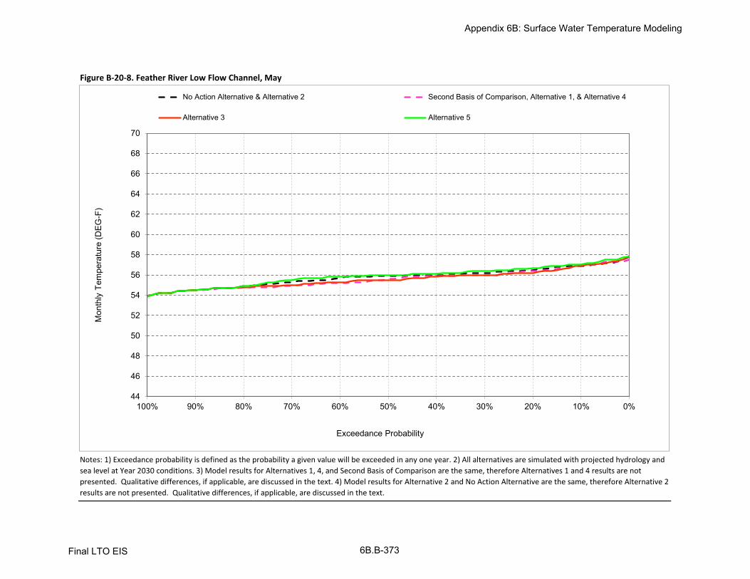
Figure B-20-8. Feather River Low Flow Channel, May
Notes: 1) Exceedance probability is defined as the probability a given value will be exceeded in any one year. 2) All alternatives are simulated with projected hydrology and
sea level at Year 2030 conditions. 3) Model results for Alternatives 1, 4, and Second Basis of Comparison are the same, therefore Alternatives 1 and 4 results are not
presented. Qualitative differences, if applicable, are discussed in the text. 4) Model results for Alternative 2 and No Action Alternative are the same, therefore Alternative 2
results are not presented. Qualitative differences, if applicable, are discussed in the text.
44
46
48
50
52
54
56
58
60
62
64
66
68
70
0%10%20%30%40%50%60%70%80%90%100%
Exceedance Probability
No Action Alternative & Alternative 2 Second Basis of Comparison, Alternative 1, & Alternative 4
Alternative 3 Alternative 5
Mon
thly
Tem
pera
ture
(DE
G-F
)
Appendix 6B: Surface Water Temperature Modeling
Final LTO EIS 6B.B-373

Figure B-20-9. Feather River Low Flow Channel, June
Notes: 1) Exceedance probability is defined as the probability a given value will be exceeded in any one year. 2) All alternatives are simulated with projected hydrology and
sea level at Year 2030 conditions. 3) Model results for Alternatives 1, 4, and Second Basis of Comparison are the same, therefore Alternatives 1 and 4 results are not
presented. Qualitative differences, if applicable, are discussed in the text. 4) Model results for Alternative 2 and No Action Alternative are the same, therefore Alternative 2
results are not presented. Qualitative differences, if applicable, are discussed in the text.
44
46
48
50
52
54
56
58
60
62
64
66
68
70
0%10%20%30%40%50%60%70%80%90%100%
Exceedance Probability
No Action Alternative & Alternative 2 Second Basis of Comparison, Alternative 1, & Alternative 4
Alternative 3 Alternative 5
Mon
thly
Tem
pera
ture
(DE
G-F
)
Appendix 6B: Surface Water Temperature Modeling
Final LTO EIS 6B.B-374

Figure B-20-10. Feather River Low Flow Channel, July
Notes: 1) Exceedance probability is defined as the probability a given value will be exceeded in any one year. 2) All alternatives are simulated with projected hydrology and
sea level at Year 2030 conditions. 3) Model results for Alternatives 1, 4, and Second Basis of Comparison are the same, therefore Alternatives 1 and 4 results are not
presented. Qualitative differences, if applicable, are discussed in the text. 4) Model results for Alternative 2 and No Action Alternative are the same, therefore Alternative 2
results are not presented. Qualitative differences, if applicable, are discussed in the text.
44
46
48
50
52
54
56
58
60
62
64
66
68
70
0%10%20%30%40%50%60%70%80%90%100%
Exceedance Probability
No Action Alternative & Alternative 2 Second Basis of Comparison, Alternative 1, & Alternative 4
Alternative 3 Alternative 5
Mon
thly
Tem
pera
ture
(DE
G-F
)
Appendix 6B: Surface Water Temperature Modeling
Final LTO EIS 6B.B-375

Figure B-20-11. Feather River Low Flow Channel, August
Notes: 1) Exceedance probability is defined as the probability a given value will be exceeded in any one year. 2) All alternatives are simulated with projected hydrology and
sea level at Year 2030 conditions. 3) Model results for Alternatives 1, 4, and Second Basis of Comparison are the same, therefore Alternatives 1 and 4 results are not
presented. Qualitative differences, if applicable, are discussed in the text. 4) Model results for Alternative 2 and No Action Alternative are the same, therefore Alternative 2
results are not presented. Qualitative differences, if applicable, are discussed in the text.
44
46
48
50
52
54
56
58
60
62
64
66
68
70
0%10%20%30%40%50%60%70%80%90%100%
Exceedance Probability
No Action Alternative & Alternative 2 Second Basis of Comparison, Alternative 1, & Alternative 4
Alternative 3 Alternative 5
Mon
thly
Tem
pera
ture
(DE
G-F
)
Appendix 6B: Surface Water Temperature Modeling
Final LTO EIS 6B.B-376

Figure B-20-12. Feather River Low Flow Channel, September
Notes: 1) Exceedance probability is defined as the probability a given value will be exceeded in any one year. 2) All alternatives are simulated with projected hydrology and
sea level at Year 2030 conditions. 3) Model results for Alternatives 1, 4, and Second Basis of Comparison are the same, therefore Alternatives 1 and 4 results are not
presented. Qualitative differences, if applicable, are discussed in the text. 4) Model results for Alternative 2 and No Action Alternative are the same, therefore Alternative 2
results are not presented. Qualitative differences, if applicable, are discussed in the text.
44
46
48
50
52
54
56
58
60
62
64
66
68
70
0%10%20%30%40%50%60%70%80%90%100%
Exceedance Probability
No Action Alternative & Alternative 2 Second Basis of Comparison, Alternative 1, & Alternative 4
Alternative 3 Alternative 5
Mon
thly
Tem
pera
ture
(DE
G-F
)
Appendix 6B: Surface Water Temperature Modeling
Final LTO EIS 6B.B-377

Oct Nov Dec Jan Feb Mar Apr May Jun Jul Aug Sep
10% 60 59 55 51 52 54 54 57 59 62 63 6020% 56 58 54 50 51 53 53 57 58 62 62 5730% 55 57 53 50 51 52 53 56 58 61 62 5740% 54 56 53 49 50 51 52 56 58 61 61 5650% 54 56 52 49 50 51 52 56 58 61 61 5560% 54 55 52 49 49 50 52 56 58 61 60 5570% 53 54 51 48 49 50 51 55 58 61 60 5580% 53 53 51 48 49 49 51 55 58 61 60 5590% 53 52 50 47 48 48 50 55 57 61 60 54
Full Simulation Periodb 55 56 52 49 50 51 52 56 58 61 61 56
Wet (32%) 52 53 49 49 49 49 51 55 58 61 60 55Above Normal (16%) 55 56 53 45 46 46 48 52 54 56 55 50Below Normal (13%) 54 56 53 50 50 52 53 56 58 61 60 56
Dry (24%) 56 56 53 49 50 52 53 56 58 61 61 57Critical (15%) 56 56 53 49 50 52 52 56 58 63 63 60
Oct Nov Dec Jan Feb Mar Apr May Jun Jul Aug Sep
10% 59 59 54 52 52 54 54 57 58 63 63 5820% 56 58 53 51 51 53 53 56 58 62 62 5730% 55 57 52 50 51 52 53 56 58 62 61 5740% 54 56 52 50 50 51 52 56 58 62 61 5650% 54 54 52 49 50 51 52 56 58 61 61 5660% 53 53 51 49 50 50 52 55 58 61 61 5670% 53 53 51 48 49 50 51 55 57 61 60 5580% 53 52 50 48 48 49 51 55 57 61 60 5590% 53 52 49 47 47 48 50 55 57 61 60 55
Full Simulation Periodb 55 55 52 49 50 51 52 56 58 62 61 56
Wet (32%) 52 52 49 49 49 50 51 55 58 61 61 56Above Normal (16%) 56 55 52 46 46 46 48 52 53 56 56 51Below Normal (13%) 54 55 52 50 50 52 53 55 57 61 61 56
Dry (24%) 55 56 52 49 50 52 53 56 58 62 61 56Critical (15%) 56 57 52 49 50 52 52 56 58 63 63 60
Oct Nov Dec Jan Feb Mar Apr May Jun Jul Aug Sep
0.1 -0.9 0.5 -1.0 0.2 0.2 0.2 -0.2 0.0 -0.5 0.2 -0.2 -1.8
0.2 0.4 -0.2 -1.1 0.2 0.4 0.3 -0.1 -0.1 -0.2 0.3 0.1 0.10.3 0.2 0.1 -0.8 0.2 0.2 0.2 0.1 -0.2 -0.4 0.5 -0.1 0.20.4 -0.1 -0.3 -0.7 0.2 0.4 -0.1 0.0 -0.1 -0.5 0.4 0.0 0.80.5 -0.1 -1.3 -0.5 0.0 0.4 0.0 0.1 -0.3 -0.3 0.3 0.2 0.90.6 -0.2 -2.3 -0.3 0.0 0.2 0.1 0.1 -0.5 -0.3 0.1 0.3 0.80.7 -0.1 -1.5 -0.6 0.2 0.1 0.2 0.1 -0.4 -0.2 0.2 0.3 0.50.8 -0.2 -0.5 -1.0 0.0 -0.1 0.3 0.2 -0.1 -0.4 0.1 0.2 0.40.9 -0.2 -0.2 -0.4 0.1 -0.4 0.0 0.2 0.0 -0.2 0.0 0.1 0.5
Full Simulation Periodb
-0.1 -0.5 -0.6 0.1 0.2 0.1 0.1 -0.2 -0.3 0.2 0.1 0.4
Wet (32%) -0.3 -1.0 -0.4 0.1 0.2 0.2 0.1 -0.1 -0.2 0.1 0.5 1.3Above Normal (16%) 0.3 -0.3 -0.9 0.1 0.2 0.0 0.0 -0.4 -0.4 0.1 0.3 0.6Below Normal (13%) 0.0 -1.2 -1.4 -0.1 0.0 0.0 0.1 -0.4 -0.7 0.2 0.4 0.0
Dry (24%) -0.2 -0.4 -0.7 0.0 0.3 0.0 0.1 -0.2 -0.2 0.4 -0.6 -0.5
Critical (15%) 0.2 0.9 -0.2 0.1 0.1 0.4 -0.1 0.0 -0.3 0.0 -0.1 -0.2
a Exceedance probability is defined as the probability a given value will be exceeded in any one year.
b Based on an 81-year simulation period.
Probability of Exceedancea
Long Term
Water Year Typesc
c As defined by the Sacramento Valley 40-30-30 Index Water Year Hydrologic Classification (SWRCB D-1641, 1999); projected to Year 2030.
Notes: 1) All alternatives are simulated with projected hydrology and sea level at Year 2030 conditions. 2) Model results for Alternatives 1, 4, and Second Basis of Comparison are the same,
therefore Second Basis of Comparison and Alternative 4 results are not presented. Qualitative differences, if applicable, are discussed in the text. 3) Model results for Alternative 2 and No Action
Alternative are the same, therefore Alternative 2 results are not presented. Qualitative differences, if applicable, are discussed in the text.
Probability of Exceedancea
Long Term
Water Year Typesc
Alternative 1 minus No Action Alternative
Statistic
Monthly Temperature (DEG-F)
Long Term
Water Year Typesc
Alternative 1
Statistic
Monthly Temperature (DEG-F)
No Action Alternative
Statistic
Monthly Temperature (DEG-F)
Probability of Exceedancea
Table B-20-1. Feather River Low Flow Channel, Monthly Temperature
Appendix 6B: Surface Water Temperature Modeling
Final LTO EIS 6B.B-378

Oct Nov Dec Jan Feb Mar Apr May Jun Jul Aug Sep
10% 60 59 55 51 52 54 54 57 59 62 63 6020% 56 58 54 50 51 53 53 57 58 62 62 5730% 55 57 53 50 51 52 53 56 58 61 62 5740% 54 56 53 49 50 51 52 56 58 61 61 5650% 54 56 52 49 50 51 52 56 58 61 61 5560% 54 55 52 49 49 50 52 56 58 61 60 5570% 53 54 51 48 49 50 51 55 58 61 60 5580% 53 53 51 48 49 49 51 55 58 61 60 5590% 53 52 50 47 48 48 50 55 57 61 60 54
Full Simulation Periodb 55 56 52 49 50 51 52 56 58 61 61 56
Wet (32%) 52 53 49 49 49 49 51 55 58 61 60 55Above Normal (16%) 55 56 53 45 46 46 48 52 54 56 55 50Below Normal (13%) 54 56 53 50 50 52 53 56 58 61 60 56
Dry (24%) 56 56 53 49 50 52 53 56 58 61 61 57Critical (15%) 56 56 53 49 50 52 52 56 58 63 63 60
Oct Nov Dec Jan Feb Mar Apr May Jun Jul Aug Sep
10% 59 59 54 52 52 54 54 57 58 63 63 5920% 56 57 53 50 51 53 53 56 58 62 62 5730% 55 56 52 50 51 52 52 56 58 61 62 5740% 54 55 52 49 50 51 52 56 58 61 61 5650% 54 54 52 49 50 51 52 56 58 61 61 5660% 53 53 51 49 49 50 52 55 58 61 60 5670% 53 53 51 48 49 50 51 55 57 61 60 5580% 53 52 50 48 49 49 51 55 57 61 60 5590% 53 52 49 47 47 48 50 55 57 61 60 55
Full Simulation Periodb 55 55 52 49 50 51 52 56 58 61 61 57
Wet (32%) 52 52 49 49 49 50 51 55 57 61 61 56Above Normal (16%) 55 55 52 46 46 46 48 52 53 56 55 51Below Normal (13%) 54 54 51 50 50 52 53 56 58 61 60 56
Dry (24%) 56 55 52 49 50 52 53 56 58 62 61 57Critical (15%) 56 56 52 49 50 52 52 56 58 63 63 60
Oct Nov Dec Jan Feb Mar Apr May Jun Jul Aug Sep
0.1 -0.8 -0.3 -1.0 0.1 0.2 0.1 -0.1 0.0 -0.5 0.3 0.0 -1.1
0.2 -0.2 -0.5 -0.7 0.0 0.2 0.1 -0.1 -0.3 -0.3 0.3 0.2 0.10.3 -0.2 -0.9 -0.7 0.1 0.1 0.1 -0.1 -0.2 -0.4 0.0 0.0 0.30.4 0.0 -0.6 -0.8 0.0 0.1 -0.1 0.0 -0.2 -0.4 0.0 0.1 0.90.5 -0.1 -1.3 -0.6 0.1 0.1 -0.1 0.1 -0.4 -0.3 0.0 0.0 1.10.6 -0.2 -2.2 -0.4 0.0 0.0 0.0 0.1 -0.4 -0.3 -0.1 0.1 1.10.7 0.0 -1.5 -0.4 0.1 0.1 0.1 0.1 -0.3 -0.2 0.0 0.1 0.80.8 -0.1 -0.5 -0.7 0.0 0.0 0.1 0.0 -0.1 -0.3 0.0 0.0 0.50.9 0.0 -0.2 -0.5 0.0 -0.3 0.0 0.1 0.0 -0.2 0.0 0.0 0.5
Full Simulation Periodb
-0.2 -0.8 -0.6 0.0 0.1 0.0 0.0 -0.2 -0.3 0.0 0.0 0.5
Wet (32%) -0.2 -1.0 -0.4 0.1 0.2 0.1 0.1 -0.1 -0.3 0.0 0.3 1.5Above Normal (16%) -0.2 -0.7 -0.7 0.1 0.1 0.0 -0.1 -0.3 -0.3 0.0 0.1 0.6Below Normal (13%) 0.0 -1.3 -1.6 -0.1 0.0 0.0 0.0 -0.3 -0.4 -0.1 -0.2 0.3
Dry (24%) 0.0 -0.7 -0.6 0.0 0.1 0.1 0.1 -0.2 -0.3 0.2 -0.1 -0.2
Critical (15%) -0.4 -0.1 -0.3 0.0 0.1 -0.1 0.0 0.1 -0.3 0.0 -0.1 -0.3
a Exceedance probability is defined as the probability a given value will be exceeded in any one year.
b Based on an 81-year simulation period.
Probability of Exceedancea
Long Term
Water Year Typesc
c As defined by the Sacramento Valley 40-30-30 Index Water Year Hydrologic Classification (SWRCB D-1641, 1999); projected to Year 2030.
Notes: 1) All alternatives are simulated with projected hydrology and sea level at Year 2030 conditions. 2) Model results for Alternatives 1, 4, and Second Basis of Comparison are the same,
therefore Alternative 1 and 4 results are not presented. Qualitative differences, if applicable, are discussed in the text. 3) Model results for Alternative 2 and No Action Alternative are the same,
therefore Alternative 2 results are not presented. Qualitative differences, if applicable, are discussed in the text.
Probability of Exceedancea
Long Term
Water Year Typesc
Alternative 3 minus No Action Alternative
Statistic
Monthly Temperature (DEG-F)
Long Term
Water Year Typesc
Alternative 3
Statistic
Monthly Temperature (DEG-F)
No Action Alternative
Statistic
Monthly Temperature (DEG-F)
Probability of Exceedancea
Table B-20-2. Feather River Low Flow Channel, Monthly Temperature
Appendix 6B: Surface Water Temperature Modeling
Final LTO EIS 6B.B-379

Oct Nov Dec Jan Feb Mar Apr May Jun Jul Aug Sep
10% 60 59 55 51 52 54 54 57 59 62 63 6020% 56 58 54 50 51 53 53 57 58 62 62 5730% 55 57 53 50 51 52 53 56 58 61 62 5740% 54 56 53 49 50 51 52 56 58 61 61 5650% 54 56 52 49 50 51 52 56 58 61 61 5560% 54 55 52 49 49 50 52 56 58 61 60 5570% 53 54 51 48 49 50 51 55 58 61 60 5580% 53 53 51 48 49 49 51 55 58 61 60 5590% 53 52 50 47 48 48 50 55 57 61 60 54
Full Simulation Periodb 55 56 52 49 50 51 52 56 58 61 61 56
Wet (32%) 52 53 49 49 49 49 51 55 58 61 60 55Above Normal (16%) 55 56 53 45 46 46 48 52 54 56 55 50Below Normal (13%) 54 56 53 50 50 52 53 56 58 61 60 56
Dry (24%) 56 56 53 49 50 52 53 56 58 61 61 57Critical (15%) 56 56 53 49 50 52 52 56 58 63 63 60
Oct Nov Dec Jan Feb Mar Apr May Jun Jul Aug Sep
10% 59 59 55 51 52 54 54 57 59 63 63 5820% 56 58 54 50 51 53 53 57 58 62 62 5730% 55 57 53 50 51 52 53 56 58 61 61 5640% 54 56 53 49 50 51 52 56 58 61 61 5650% 54 55 52 49 50 51 52 56 58 61 60 5560% 54 55 52 49 49 50 52 56 58 61 60 5570% 53 54 51 48 49 50 51 56 58 61 60 5580% 53 53 50 48 49 49 51 55 58 61 60 5590% 53 53 50 47 48 48 50 55 57 61 60 54
Full Simulation Periodb 55 55 52 49 50 51 52 56 58 61 61 56
Wet (32%) 52 53 49 49 49 49 51 55 58 61 60 55Above Normal (16%) 55 56 53 45 46 46 48 52 54 56 55 50Below Normal (13%) 54 56 53 50 50 52 53 56 58 61 60 56
Dry (24%) 55 56 53 49 50 52 53 56 58 61 61 57Critical (15%) 56 56 53 49 50 52 53 57 59 63 63 60
Oct Nov Dec Jan Feb Mar Apr May Jun Jul Aug Sep
0.1 -0.9 -0.1 -0.1 0.0 0.0 0.0 0.1 0.1 0.1 0.2 0.0 -1.3
0.2 -0.4 -0.2 0.1 0.0 0.0 0.1 0.0 0.2 0.0 -0.1 0.0 0.00.3 0.0 0.1 0.0 0.0 0.1 0.1 0.1 0.2 0.0 -0.1 -0.1 -0.4
0.4 0.2 0.0 -0.1 0.0 0.0 0.0 0.0 0.1 0.0 0.0 -0.4 0.00.5 0.1 -0.1 0.0 0.0 0.0 -0.1 0.0 0.1 0.1 0.0 -0.1 0.00.6 0.0 -0.3 0.1 0.0 0.0 0.0 0.0 0.1 0.1 -0.1 0.0 0.00.7 -0.1 -0.2 0.0 0.0 0.0 0.0 0.0 0.2 0.1 0.0 0.0 0.00.8 0.0 0.0 -0.5 0.0 0.0 -0.1 0.0 0.0 0.0 -0.1 0.0 0.00.9 0.0 0.2 0.0 -0.1 0.0 0.0 0.0 0.0 0.0 0.0 0.0 0.0
Full Simulation Periodb
-0.1 -0.1 0.0 0.0 0.0 0.0 0.0 0.1 0.0 0.0 -0.1 -0.1
Wet (32%) 0.0 0.0 0.0 0.0 0.0 0.0 0.0 0.0 0.0 0.0 0.0 0.0Above Normal (16%) -0.1 0.0 0.0 0.0 0.0 0.0 0.0 0.1 0.0 0.0 0.0 0.0Below Normal (13%) -0.2 -0.2 0.0 0.0 0.1 0.0 0.0 0.2 0.1 0.0 -0.1 -0.1
Dry (24%) -0.2 -0.3 0.0 0.0 0.0 0.0 0.0 0.3 0.0 0.0 -0.1 -0.1
Critical (15%) -0.1 -0.1 0.0 0.0 0.0 0.0 0.0 0.2 0.1 -0.1 -0.1 -0.5
a Exceedance probability is defined as the probability a given value will be exceeded in any one year.
b Based on an 81-year simulation period.
Probability of Exceedancea
Long Term
Water Year Typesc
c As defined by the Sacramento Valley 40-30-30 Index Water Year Hydrologic Classification (SWRCB D-1641, 1999); projected to Year 2030.
Notes: 1) All alternatives are simulated with projected hydrology and sea level at Year 2030 conditions. 2) Model results for Alternatives 1, 4, and Second Basis of Comparison are the same,
therefore Alternative 1 and 4 results are not presented. Qualitative differences, if applicable, are discussed in the text. 3) Model results for Alternative 2 and No Action Alternative are the same,
therefore Alternative 2 results are not presented. Qualitative differences, if applicable, are discussed in the text.
Probability of Exceedancea
Long Term
Water Year Typesc
Alternative 5 minus No Action Alternative
Statistic
Monthly Temperature (DEG-F)
Long Term
Water Year Typesc
Alternative 5
Statistic
Monthly Temperature (DEG-F)
No Action Alternative
Statistic
Monthly Temperature (DEG-F)
Probability of Exceedancea
Table B-20-3. Feather River Low Flow Channel, Monthly Temperature
Appendix 6B: Surface Water Temperature Modeling
Final LTO EIS 6B.B-380

Oct Nov Dec Jan Feb Mar Apr May Jun Jul Aug Sep
10% 59 59 54 52 52 54 54 57 58 63 63 5820% 56 58 53 51 51 53 53 56 58 62 62 5730% 55 57 52 50 51 52 53 56 58 62 61 5740% 54 56 52 50 50 51 52 56 58 62 61 5650% 54 54 52 49 50 51 52 56 58 61 61 5660% 53 53 51 49 50 50 52 55 58 61 61 5670% 53 53 51 48 49 50 51 55 57 61 60 5580% 53 52 50 48 48 49 51 55 57 61 60 5590% 53 52 49 47 47 48 50 55 57 61 60 55
Full Simulation Periodb 55 55 52 49 50 51 52 56 58 62 61 56
Wet (32%) 52 52 49 49 49 50 51 55 58 61 61 56Above Normal (16%) 56 55 52 46 46 46 48 52 53 56 56 51Below Normal (13%) 54 55 52 50 50 52 53 55 57 61 61 56
Dry (24%) 55 56 52 49 50 52 53 56 58 62 61 56Critical (15%) 56 57 52 49 50 52 52 56 58 63 63 60
Oct Nov Dec Jan Feb Mar Apr May Jun Jul Aug Sep
10% 60 59 55 51 52 54 54 57 59 62 63 6020% 56 58 54 50 51 53 53 57 58 62 62 5730% 55 57 53 50 51 52 53 56 58 61 62 5740% 54 56 53 49 50 51 52 56 58 61 61 5650% 54 56 52 49 50 51 52 56 58 61 61 5560% 54 55 52 49 49 50 52 56 58 61 60 5570% 53 54 51 48 49 50 51 55 58 61 60 5580% 53 53 51 48 49 49 51 55 58 61 60 5590% 53 52 50 47 48 48 50 55 57 61 60 54
Full Simulation Periodb 55 56 52 49 50 51 52 56 58 61 61 56
Wet (32%) 52 53 49 49 49 49 51 55 58 61 60 55Above Normal (16%) 55 56 53 45 46 46 48 52 54 56 55 50Below Normal (13%) 54 56 53 50 50 52 53 56 58 61 60 56
Dry (24%) 56 56 53 49 50 52 53 56 58 61 61 57Critical (15%) 56 56 53 49 50 52 52 56 58 63 63 60
Oct Nov Dec Jan Feb Mar Apr May Jun Jul Aug Sep
0.1 0.9 -0.5 1.0 -0.2 -0.2 -0.2 0.2 0.0 0.5 -0.2 0.2 1.80.2 -0.4 0.2 1.1 -0.2 -0.4 -0.3 0.1 0.1 0.2 -0.3 -0.1 -0.1
0.3 -0.2 -0.1 0.8 -0.2 -0.2 -0.2 -0.1 0.2 0.4 -0.5 0.1 -0.2
0.4 0.1 0.3 0.7 -0.2 -0.4 0.1 0.0 0.1 0.5 -0.4 0.0 -0.8
0.5 0.1 1.3 0.5 0.0 -0.4 0.0 -0.1 0.3 0.3 -0.3 -0.2 -0.9
0.6 0.2 2.3 0.3 0.0 -0.2 -0.1 -0.1 0.5 0.3 -0.1 -0.3 -0.8
0.7 0.1 1.5 0.6 -0.2 -0.1 -0.2 -0.1 0.4 0.2 -0.2 -0.3 -0.5
0.8 0.2 0.5 1.0 0.0 0.1 -0.3 -0.2 0.1 0.4 -0.1 -0.2 -0.4
0.9 0.2 0.2 0.4 -0.1 0.4 0.0 -0.2 0.0 0.2 0.0 -0.1 -0.5
Full Simulation Periodb 0.1 0.5 0.6 -0.1 -0.2 -0.1 -0.1 0.2 0.3 -0.2 -0.1 -0.4
Wet (32%) 0.3 1.0 0.4 -0.1 -0.2 -0.2 -0.1 0.1 0.2 -0.1 -0.5 -1.3
Above Normal (16%) -0.3 0.3 0.9 -0.1 -0.2 0.0 0.0 0.4 0.4 -0.1 -0.3 -0.6
Below Normal (13%) 0.0 1.2 1.4 0.1 0.0 0.0 -0.1 0.4 0.7 -0.2 -0.4 0.0Dry (24%) 0.2 0.4 0.7 0.0 -0.3 0.0 -0.1 0.2 0.2 -0.4 0.6 0.5
Critical (15%) -0.2 -0.9 0.2 -0.1 -0.1 -0.4 0.1 0.0 0.3 0.0 0.1 0.2
a Exceedance probability is defined as the probability a given value will be exceeded in any one year.
b Based on an 81-year simulation period.
Probability of Exceedancea
Long Term
Water Year Typesc
c As defined by the Sacramento Valley 40-30-30 Index Water Year Hydrologic Classification (SWRCB D-1641, 1999); projected to Year 2030.
Notes: 1) All alternatives are simulated with projected hydrology and sea level at Year 2030 conditions. 2) Model results for Alternatives 1, 4, and Second Basis of Comparison are the same,
therefore Alternative 1 and 4 results are not presented. Qualitative differences, if applicable, are discussed in the text. 3) Model results for Alternative 2 and No Action Alternative are the same,
therefore Alternative 2 results are not presented. Qualitative differences, if applicable, are discussed in the text.
Probability of Exceedancea
Long Term
Water Year Typesc
No Action Alternative minus Second Basis of Comparison
Statistic
Monthly Temperature (DEG-F)
Long Term
Water Year Typesc
No Action Alternative
Statistic
Monthly Temperature (DEG-F)
Second Basis of Comparison
Statistic
Monthly Temperature (DEG-F)
Probability of Exceedancea
Table B-20-4. Feather River Low Flow Channel, Monthly Temperature
Appendix 6B: Surface Water Temperature Modeling
Final LTO EIS 6B.B-381

Oct Nov Dec Jan Feb Mar Apr May Jun Jul Aug Sep
10% 59 59 54 52 52 54 54 57 58 63 63 5820% 56 58 53 51 51 53 53 56 58 62 62 5730% 55 57 52 50 51 52 53 56 58 62 61 5740% 54 56 52 50 50 51 52 56 58 62 61 5650% 54 54 52 49 50 51 52 56 58 61 61 5660% 53 53 51 49 50 50 52 55 58 61 61 5670% 53 53 51 48 49 50 51 55 57 61 60 5580% 53 52 50 48 48 49 51 55 57 61 60 5590% 53 52 49 47 47 48 50 55 57 61 60 55
Full Simulation Periodb 55 55 52 49 50 51 52 56 58 62 61 56
Wet (32%) 52 52 49 49 49 50 51 55 58 61 61 56Above Normal (16%) 56 55 52 46 46 46 48 52 53 56 56 51Below Normal (13%) 54 55 52 50 50 52 53 55 57 61 61 56
Dry (24%) 55 56 52 49 50 52 53 56 58 62 61 56Critical (15%) 56 57 52 49 50 52 52 56 58 63 63 60
Oct Nov Dec Jan Feb Mar Apr May Jun Jul Aug Sep
10% 59 59 54 52 52 54 54 57 58 63 63 5920% 56 57 53 50 51 53 53 56 58 62 62 5730% 55 56 52 50 51 52 52 56 58 61 62 5740% 54 55 52 49 50 51 52 56 58 61 61 5650% 54 54 52 49 50 51 52 56 58 61 61 5660% 53 53 51 49 49 50 52 55 58 61 60 5670% 53 53 51 48 49 50 51 55 57 61 60 5580% 53 52 50 48 49 49 51 55 57 61 60 5590% 53 52 49 47 47 48 50 55 57 61 60 55
Full Simulation Periodb 55 55 52 49 50 51 52 56 58 61 61 57
Wet (32%) 52 52 49 49 49 50 51 55 57 61 61 56Above Normal (16%) 55 55 52 46 46 46 48 52 53 56 55 51Below Normal (13%) 54 54 51 50 50 52 53 56 58 61 60 56
Dry (24%) 56 55 52 49 50 52 53 56 58 62 61 57Critical (15%) 56 56 52 49 50 52 52 56 58 63 63 60
Oct Nov Dec Jan Feb Mar Apr May Jun Jul Aug Sep
0.1 0.1 -0.8 0.0 -0.1 0.0 -0.1 0.1 0.0 0.0 0.1 0.2 0.70.2 -0.6 -0.3 0.4 -0.2 -0.2 -0.2 0.0 -0.2 -0.1 0.0 0.1 0.00.3 -0.4 -1.0 0.1 -0.1 -0.1 -0.1 -0.2 0.0 0.0 -0.5 0.1 0.10.4 0.1 -0.3 -0.1 -0.2 -0.3 0.0 0.0 -0.1 0.1 -0.4 0.1 0.10.5 0.0 0.0 -0.1 0.1 -0.3 -0.1 0.0 -0.1 0.0 -0.3 -0.2 0.20.6 0.0 0.1 -0.1 0.0 -0.2 -0.1 0.0 0.1 0.0 -0.2 -0.2 0.30.7 0.1 0.0 0.2 -0.1 0.0 -0.1 0.0 0.1 0.0 -0.2 -0.2 0.30.8 0.1 0.0 0.3 0.0 0.1 -0.2 -0.2 0.0 0.1 -0.1 -0.2 0.10.9 0.2 0.0 -0.1 -0.1 0.1 0.0 -0.1 0.0 0.0 0.0 -0.1 0.0
Full Simulation Periodb
-0.1 -0.3 0.0 -0.1 -0.1 -0.1 0.0 0.0 0.0 -0.1 0.0 0.2
Wet (32%) 0.1 0.1 0.0 -0.1 0.0 -0.1 0.0 0.0 -0.1 -0.1 -0.2 0.2Above Normal (16%) -0.5 -0.4 0.2 -0.1 -0.1 0.0 -0.1 0.0 0.1 -0.1 -0.2 0.0
Below Normal (13%) 0.0 0.0 -0.2 0.0 0.0 0.0 0.0 0.1 0.2 -0.2 -0.7 0.3Dry (24%) 0.2 -0.3 0.1 0.0 -0.2 0.0 -0.1 -0.1 -0.1 -0.2 0.5 0.3
Critical (15%) -0.5 -1.0 -0.1 -0.1 0.0 -0.5 0.0 0.1 0.0 0.0 0.0 -0.2
a Exceedance probability is defined as the probability a given value will be exceeded in any one year.
b Based on an 81-year simulation period.
Probability of Exceedancea
Long Term
Water Year Typesc
c As defined by the Sacramento Valley 40-30-30 Index Water Year Hydrologic Classification (SWRCB D-1641, 1999); projected to Year 2030.
Notes: 1) All alternatives are simulated with projected hydrology and sea level at Year 2030 conditions. 2) Model results for Alternatives 1, 4, and Second Basis of Comparison are the same,
therefore Alternative 1 and 4 results are not presented. Qualitative differences, if applicable, are discussed in the text. 3) Model results for Alternative 2 and No Action Alternative are the same,
therefore Alternative 2 results are not presented. Qualitative differences, if applicable, are discussed in the text.
Probability of Exceedancea
Long Term
Water Year Typesc
Alternative 3 minus Second Basis of Comparison
Statistic
Monthly Temperature (DEG-F)
Long Term
Water Year Typesc
Alternative 3
Statistic
Monthly Temperature (DEG-F)
Second Basis of Comparison
Statistic
Monthly Temperature (DEG-F)
Probability of Exceedancea
Table B-20-5. Feather River Low Flow Channel, Monthly Temperature
Appendix 6B: Surface Water Temperature Modeling
Final LTO EIS 6B.B-382

Oct Nov Dec Jan Feb Mar Apr May Jun Jul Aug Sep
10% 59 59 54 52 52 54 54 57 58 63 63 5820% 56 58 53 51 51 53 53 56 58 62 62 5730% 55 57 52 50 51 52 53 56 58 62 61 5740% 54 56 52 50 50 51 52 56 58 62 61 5650% 54 54 52 49 50 51 52 56 58 61 61 5660% 53 53 51 49 50 50 52 55 58 61 61 5670% 53 53 51 48 49 50 51 55 57 61 60 5580% 53 52 50 48 48 49 51 55 57 61 60 5590% 53 52 49 47 47 48 50 55 57 61 60 55
Full Simulation Periodb 55 55 52 49 50 51 52 56 58 62 61 56
Wet (32%) 52 52 49 49 49 50 51 55 58 61 61 56Above Normal (16%) 56 55 52 46 46 46 48 52 53 56 56 51Below Normal (13%) 54 55 52 50 50 52 53 55 57 61 61 56
Dry (24%) 55 56 52 49 50 52 53 56 58 62 61 56Critical (15%) 56 57 52 49 50 52 52 56 58 63 63 60
Oct Nov Dec Jan Feb Mar Apr May Jun Jul Aug Sep
10% 59 59 55 51 52 54 54 57 59 63 63 5820% 56 58 54 50 51 53 53 57 58 62 62 5730% 55 57 53 50 51 52 53 56 58 61 61 5640% 54 56 53 49 50 51 52 56 58 61 61 5650% 54 55 52 49 50 51 52 56 58 61 60 5560% 54 55 52 49 49 50 52 56 58 61 60 5570% 53 54 51 48 49 50 51 56 58 61 60 5580% 53 53 50 48 49 49 51 55 58 61 60 5590% 53 53 50 47 48 48 50 55 57 61 60 54
Full Simulation Periodb 55 55 52 49 50 51 52 56 58 61 61 56
Wet (32%) 52 53 49 49 49 49 51 55 58 61 60 55Above Normal (16%) 55 56 53 45 46 46 48 52 54 56 55 50Below Normal (13%) 54 56 53 50 50 52 53 56 58 61 60 56
Dry (24%) 55 56 53 49 50 52 53 56 58 61 61 57Critical (15%) 56 56 53 49 50 52 53 57 59 63 63 60
Oct Nov Dec Jan Feb Mar Apr May Jun Jul Aug Sep
0.1 0.0 -0.6 0.9 -0.2 -0.2 -0.2 0.3 0.1 0.6 0.0 0.2 0.50.2 -0.8 0.0 1.2 -0.2 -0.4 -0.2 0.1 0.3 0.2 -0.4 -0.1 -0.1
0.3 -0.2 0.0 0.8 -0.2 -0.1 -0.1 0.0 0.4 0.4 -0.6 0.0 -0.6
0.4 0.3 0.3 0.6 -0.2 -0.4 0.1 0.0 0.2 0.5 -0.4 -0.4 -0.8
0.5 0.2 1.2 0.5 0.0 -0.4 -0.1 -0.1 0.4 0.4 -0.3 -0.3 -0.9
0.6 0.2 2.0 0.4 0.0 -0.2 -0.1 -0.1 0.6 0.4 -0.2 -0.3 -0.8
0.7 0.0 1.3 0.6 -0.2 -0.1 -0.2 -0.1 0.6 0.3 -0.2 -0.3 -0.5
0.8 0.2 0.5 0.5 0.0 0.1 -0.4 -0.2 0.1 0.4 -0.2 -0.2 -0.4
0.9 0.2 0.4 0.4 -0.2 0.4 0.0 -0.2 0.0 0.2 0.0 -0.1 -0.5
Full Simulation Periodb
0.0 0.4 0.6 -0.1 -0.2 -0.1 -0.1 0.3 0.3 -0.2 -0.2 -0.5
Wet (32%) 0.3 1.1 0.4 -0.2 -0.2 -0.2 -0.1 0.1 0.2 -0.1 -0.5 -1.2
Above Normal (16%) -0.4 0.2 0.8 -0.2 -0.2 0.0 0.0 0.4 0.4 -0.1 -0.3 -0.6
Below Normal (13%) -0.2 1.0 1.5 0.1 0.1 0.0 -0.1 0.6 0.7 -0.2 -0.6 -0.1
Dry (24%) 0.1 0.2 0.7 0.0 -0.3 0.0 -0.1 0.4 0.2 -0.4 0.6 0.4Critical (15%) -0.3 -1.0 0.2 -0.1 -0.1 -0.4 0.1 0.2 0.3 0.0 0.0 -0.3
a Exceedance probability is defined as the probability a given value will be exceeded in any one year.
b Based on an 81-year simulation period.
Probability of Exceedancea
Long Term
Water Year Typesc
c As defined by the Sacramento Valley 40-30-30 Index Water Year Hydrologic Classification (SWRCB D-1641, 1999); projected to Year 2030.
Notes: 1) All alternatives are simulated with projected hydrology and sea level at Year 2030 conditions. 2) Model results for Alternatives 1, 4, and Second Basis of Comparison are the same,
therefore Alternative 1 and 4 results are not presented. Qualitative differences, if applicable, are discussed in the text. 3) Model results for Alternative 2 and No Action Alternative are the same,
therefore Alternative 2 results are not presented. Qualitative differences, if applicable, are discussed in the text.
Probability of Exceedancea
Long Term
Water Year Typesc
Alternative 5 minus Second Basis of Comparison
Statistic
Monthly Temperature (DEG-F)
Long Term
Water Year Typesc
Alternative 5
Statistic
Monthly Temperature (DEG-F)
Second Basis of Comparison
Statistic
Monthly Temperature (DEG-F)
Probability of Exceedancea
Table B-20-6. Feather River Low Flow Channel, Monthly Temperature
Appendix 6B: Surface Water Temperature Modeling
Final LTO EIS 6B.B-384

B.21. Feather River at Robinson Riffle
Appendix 6B: Surface Water Temperature Modeling
Final LTO EIS 6B.B-385

Figure B-21-1. Feather River at Robinson Riffle, October
Notes: 1) Exceedance probability is defined as the probability a given value will be exceeded in any one year. 2) All alternatives are simulated with projected hydrology and
sea level at Year 2030 conditions. 3) Model results for Alternatives 1, 4, and Second Basis of Comparison are the same, therefore Alternatives 1 and 4 results are not
presented. Qualitative differences, if applicable, are discussed in the text. 4) Model results for Alternative 2 and No Action Alternative are the same, therefore Alternative 2
results are not presented. Qualitative differences, if applicable, are discussed in the text.
4446485052545658606264666870727476788082
0%10%20%30%40%50%60%70%80%90%100%
Exceedance Probability
No Action Alternative & Alternative 2 Second Basis of Comparison, Alternative 1, & Alternative 4
Alternative 3 Alternative 5
Mon
thly
Tem
pera
ture
(DE
G-F
)
Appendix 6B: Surface Water Temperature Modeling
Final LTO EIS 6B.B-386

Figure B-21-2. Feather River at Robinson Riffle, November
Notes: 1) Exceedance probability is defined as the probability a given value will be exceeded in any one year. 2) All alternatives are simulated with projected hydrology and
sea level at Year 2030 conditions. 3) Model results for Alternatives 1, 4, and Second Basis of Comparison are the same, therefore Alternatives 1 and 4 results are not
presented. Qualitative differences, if applicable, are discussed in the text. 4) Model results for Alternative 2 and No Action Alternative are the same, therefore Alternative 2
results are not presented. Qualitative differences, if applicable, are discussed in the text.
4446485052545658606264666870727476788082
0%10%20%30%40%50%60%70%80%90%100%
Exceedance Probability
No Action Alternative & Alternative 2 Second Basis of Comparison, Alternative 1, & Alternative 4
Alternative 3 Alternative 5
Mon
thly
Tem
pera
ture
(DE
G-F
)
Appendix 6B: Surface Water Temperature Modeling
Final LTO EIS 6B.B-387

Figure B-21-3. Feather River at Robinson Riffle, December
Notes: 1) Exceedance probability is defined as the probability a given value will be exceeded in any one year. 2) All alternatives are simulated with projected hydrology and
sea level at Year 2030 conditions. 3) Model results for Alternatives 1, 4, and Second Basis of Comparison are the same, therefore Alternatives 1 and 4 results are not
presented. Qualitative differences, if applicable, are discussed in the text. 4) Model results for Alternative 2 and No Action Alternative are the same, therefore Alternative 2
results are not presented. Qualitative differences, if applicable, are discussed in the text.
4446485052545658606264666870727476788082
0%10%20%30%40%50%60%70%80%90%100%
Exceedance Probability
No Action Alternative & Alternative 2 Second Basis of Comparison, Alternative 1, & Alternative 4
Alternative 3 Alternative 5
Mon
thly
Tem
pera
ture
(DE
G-F
)
Appendix 6B: Surface Water Temperature Modeling
Final LTO EIS 6B.B-388

Figure B-21-4. Feather River at Robinson Riffle, January
Notes: 1) Exceedance probability is defined as the probability a given value will be exceeded in any one year. 2) All alternatives are simulated with projected hydrology and
sea level at Year 2030 conditions. 3) Model results for Alternatives 1, 4, and Second Basis of Comparison are the same, therefore Alternatives 1 and 4 results are not
presented. Qualitative differences, if applicable, are discussed in the text. 4) Model results for Alternative 2 and No Action Alternative are the same, therefore Alternative 2
results are not presented. Qualitative differences, if applicable, are discussed in the text.
4446485052545658606264666870727476788082
0%10%20%30%40%50%60%70%80%90%100%
Exceedance Probability
No Action Alternative & Alternative 2 Second Basis of Comparison, Alternative 1, & Alternative 4
Alternative 3 Alternative 5
Mon
thly
Tem
pera
ture
(DE
G-F
)
Appendix 6B: Surface Water Temperature Modeling
Final LTO EIS 6B.B-389

Figure B-21-5. Feather River at Robinson Riffle, February
Notes: 1) Exceedance probability is defined as the probability a given value will be exceeded in any one year. 2) All alternatives are simulated with projected hydrology and
sea level at Year 2030 conditions. 3) Model results for Alternatives 1, 4, and Second Basis of Comparison are the same, therefore Alternatives 1 and 4 results are not
presented. Qualitative differences, if applicable, are discussed in the text. 4) Model results for Alternative 2 and No Action Alternative are the same, therefore Alternative 2
results are not presented. Qualitative differences, if applicable, are discussed in the text.
4446485052545658606264666870727476788082
0%10%20%30%40%50%60%70%80%90%100%
Exceedance Probability
No Action Alternative & Alternative 2 Second Basis of Comparison, Alternative 1, & Alternative 4
Alternative 3 Alternative 5
Mon
thly
Tem
pera
ture
(DE
G-F
)
Appendix 6B: Surface Water Temperature Modeling
Final LTO EIS 6B.B-390

Figure B-21-6. Feather River at Robinson Riffle, March
Notes: 1) Exceedance probability is defined as the probability a given value will be exceeded in any one year. 2) All alternatives are simulated with projected hydrology and
sea level at Year 2030 conditions. 3) Model results for Alternatives 1, 4, and Second Basis of Comparison are the same, therefore Alternatives 1 and 4 results are not
presented. Qualitative differences, if applicable, are discussed in the text. 4) Model results for Alternative 2 and No Action Alternative are the same, therefore Alternative 2
results are not presented. Qualitative differences, if applicable, are discussed in the text.
4446485052545658606264666870727476788082
0%10%20%30%40%50%60%70%80%90%100%
Exceedance Probability
No Action Alternative & Alternative 2 Second Basis of Comparison, Alternative 1, & Alternative 4
Alternative 3 Alternative 5
Mon
thly
Tem
pera
ture
(DE
G-F
)
Appendix 6B: Surface Water Temperature Modeling
Final LTO EIS 6B.B-391

Figure B-21-7. Feather River at Robinson Riffle, April
Notes: 1) Exceedance probability is defined as the probability a given value will be exceeded in any one year. 2) All alternatives are simulated with projected hydrology and
sea level at Year 2030 conditions. 3) Model results for Alternatives 1, 4, and Second Basis of Comparison are the same, therefore Alternatives 1 and 4 results are not
presented. Qualitative differences, if applicable, are discussed in the text. 4) Model results for Alternative 2 and No Action Alternative are the same, therefore Alternative 2
results are not presented. Qualitative differences, if applicable, are discussed in the text.
4446485052545658606264666870727476788082
0%10%20%30%40%50%60%70%80%90%100%
Exceedance Probability
No Action Alternative & Alternative 2 Second Basis of Comparison, Alternative 1, & Alternative 4
Alternative 3 Alternative 5
Mon
thly
Tem
pera
ture
(DE
G-F
)
Appendix 6B: Surface Water Temperature Modeling
Final LTO EIS 6B.B-392

Figure B-21-8. Feather River at Robinson Riffle, May
Notes: 1) Exceedance probability is defined as the probability a given value will be exceeded in any one year. 2) All alternatives are simulated with projected hydrology and
sea level at Year 2030 conditions. 3) Model results for Alternatives 1, 4, and Second Basis of Comparison are the same, therefore Alternatives 1 and 4 results are not
presented. Qualitative differences, if applicable, are discussed in the text. 4) Model results for Alternative 2 and No Action Alternative are the same, therefore Alternative 2
results are not presented. Qualitative differences, if applicable, are discussed in the text.
4446485052545658606264666870727476788082
0%10%20%30%40%50%60%70%80%90%100%
Exceedance Probability
No Action Alternative & Alternative 2 Second Basis of Comparison, Alternative 1, & Alternative 4
Alternative 3 Alternative 5
Mon
thly
Tem
pera
ture
(DE
G-F
)
Appendix 6B: Surface Water Temperature Modeling
Final LTO EIS 6B.B-393

Figure B-21-9. Feather River at Robinson Riffle, June
Notes: 1) Exceedance probability is defined as the probability a given value will be exceeded in any one year. 2) All alternatives are simulated with projected hydrology and
sea level at Year 2030 conditions. 3) Model results for Alternatives 1, 4, and Second Basis of Comparison are the same, therefore Alternatives 1 and 4 results are not
presented. Qualitative differences, if applicable, are discussed in the text. 4) Model results for Alternative 2 and No Action Alternative are the same, therefore Alternative 2
results are not presented. Qualitative differences, if applicable, are discussed in the text.
4446485052545658606264666870727476788082
0%10%20%30%40%50%60%70%80%90%100%
Exceedance Probability
No Action Alternative & Alternative 2 Second Basis of Comparison, Alternative 1, & Alternative 4
Alternative 3 Alternative 5
Mon
thly
Tem
pera
ture
(DE
G-F
)
Appendix 6B: Surface Water Temperature Modeling
Final LTO EIS 6B.B-394

Figure B-21-10. Feather River at Robinson Riffle, July
Notes: 1) Exceedance probability is defined as the probability a given value will be exceeded in any one year. 2) All alternatives are simulated with projected hydrology and
sea level at Year 2030 conditions. 3) Model results for Alternatives 1, 4, and Second Basis of Comparison are the same, therefore Alternatives 1 and 4 results are not
presented. Qualitative differences, if applicable, are discussed in the text. 4) Model results for Alternative 2 and No Action Alternative are the same, therefore Alternative 2
results are not presented. Qualitative differences, if applicable, are discussed in the text.
4446485052545658606264666870727476788082
0%10%20%30%40%50%60%70%80%90%100%
Exceedance Probability
No Action Alternative & Alternative 2 Second Basis of Comparison, Alternative 1, & Alternative 4
Alternative 3 Alternative 5
Mon
thly
Tem
pera
ture
(DE
G-F
)
Appendix 6B: Surface Water Temperature Modeling
Final LTO EIS 6B.B-395

Figure B-21-11. Feather River at Robinson Riffle, August
Notes: 1) Exceedance probability is defined as the probability a given value will be exceeded in any one year. 2) All alternatives are simulated with projected hydrology and
sea level at Year 2030 conditions. 3) Model results for Alternatives 1, 4, and Second Basis of Comparison are the same, therefore Alternatives 1 and 4 results are not
presented. Qualitative differences, if applicable, are discussed in the text. 4) Model results for Alternative 2 and No Action Alternative are the same, therefore Alternative 2
results are not presented. Qualitative differences, if applicable, are discussed in the text.
4446485052545658606264666870727476788082
0%10%20%30%40%50%60%70%80%90%100%
Exceedance Probability
No Action Alternative & Alternative 2 Second Basis of Comparison, Alternative 1, & Alternative 4
Alternative 3 Alternative 5
Mon
thly
Tem
pera
ture
(DE
G-F
)
Appendix 6B: Surface Water Temperature Modeling
Final LTO EIS 6B.B-396

Figure B-21-12. Feather River at Robinson Riffle, September
Notes: 1) Exceedance probability is defined as the probability a given value will be exceeded in any one year. 2) All alternatives are simulated with projected hydrology and
sea level at Year 2030 conditions. 3) Model results for Alternatives 1, 4, and Second Basis of Comparison are the same, therefore Alternatives 1 and 4 results are not
presented. Qualitative differences, if applicable, are discussed in the text. 4) Model results for Alternative 2 and No Action Alternative are the same, therefore Alternative 2
results are not presented. Qualitative differences, if applicable, are discussed in the text.
4446485052545658606264666870727476788082
0%10%20%30%40%50%60%70%80%90%100%
Exceedance Probability
No Action Alternative & Alternative 2 Second Basis of Comparison, Alternative 1, & Alternative 4
Alternative 3 Alternative 5
Mon
thly
Tem
pera
ture
(DE
G-F
)
Appendix 6B: Surface Water Temperature Modeling
Final LTO EIS 6B.B-397

Oct Nov Dec Jan Feb Mar Apr May Jun Jul Aug Sep
10% 62 58 52 50 53 57 60 67 71 73 73 6720% 60 57 51 50 52 56 59 65 71 72 72 6530% 60 56 51 49 52 55 58 64 70 71 71 6540% 59 56 51 49 52 55 58 64 69 70 70 6450% 59 55 50 48 51 54 58 64 69 70 70 6360% 59 55 50 48 51 53 57 63 68 69 69 6270% 58 54 49 47 50 52 57 62 67 69 68 6280% 57 54 49 46 49 52 56 61 67 68 68 6190% 57 52 48 45 49 50 55 60 66 68 67 61
Full Simulation Periodb 59 55 50 48 51 54 57 63 68 70 70 63
Wet (32%) 57 53 48 48 50 52 56 62 67 70 69 61Above Normal (16%) 60 56 50 45 47 49 54 59 63 63 62 57Below Normal (13%) 59 55 50 48 51 55 59 64 69 69 69 65
Dry (24%) 59 56 50 47 51 55 58 64 69 70 71 64Critical (15%) 60 56 50 48 52 55 58 64 70 74 73 66
Oct Nov Dec Jan Feb Mar Apr May Jun Jul Aug Sep
10% 62 58 52 50 53 57 60 66 70 75 74 6720% 61 57 51 50 53 56 59 65 69 73 73 6730% 60 56 50 49 52 55 58 64 69 72 72 6540% 60 55 50 49 51 55 58 64 68 72 71 6550% 59 55 50 48 51 54 58 63 68 71 71 6460% 59 54 49 48 51 53 57 63 67 70 70 6470% 58 53 49 47 50 52 57 62 66 70 70 6480% 57 53 48 46 49 52 56 61 66 69 69 6390% 57 52 47 45 49 50 55 60 65 68 67 63
Full Simulation Periodb 59 55 49 48 51 54 57 63 68 71 71 65
Wet (32%) 56 52 48 48 50 52 56 62 67 70 70 65Above Normal (16%) 60 55 50 45 47 49 53 59 62 63 63 59Below Normal (13%) 59 54 49 48 51 55 59 63 67 70 71 65
Dry (24%) 60 55 49 47 51 55 58 64 68 72 71 65Critical (15%) 60 56 49 48 52 55 58 64 69 75 73 67
Oct Nov Dec Jan Feb Mar Apr May Jun Jul Aug Sep
0.1 -0.5 -0.2 -0.4 -0.1 0.0 0.1 0.2 -0.6 -0.4 1.3 0.3 0.60.2 0.7 0.2 -0.3 0.0 0.3 0.0 0.2 -0.6 -1.6 1.1 0.7 1.10.3 0.2 -0.2 -0.4 0.3 0.0 -0.1 0.0 -0.2 -1.3 1.4 0.4 0.80.4 0.3 -0.2 -0.5 0.1 -0.2 0.0 0.1 -0.1 -0.9 1.7 0.8 1.30.5 0.0 -0.4 -0.4 0.0 0.1 -0.2 0.0 -0.5 -1.0 1.2 0.6 1.50.6 -0.1 -0.7 -0.5 0.1 0.0 -0.4 0.2 -0.5 -1.1 0.8 0.8 1.90.7 -0.3 -1.0 -0.5 0.2 0.1 -0.1 -0.1 -0.3 -1.0 0.6 1.3 2.00.8 0.1 -0.8 -0.3 -0.1 0.0 0.1 0.0 0.0 -0.7 0.8 0.8 2.10.9 0.2 0.0 -0.5 0.0 -0.1 0.1 0.0 0.0 -0.8 0.1 0.2 2.2
Full Simulation Periodb 0.1 -0.3 -0.4 0.1 0.0 0.0 0.1 -0.2 -0.9 0.9 0.5 1.5
Wet (32%) -0.2 -0.6 -0.1 0.2 0.1 0.0 0.0 0.1 -0.3 0.6 0.9 3.4Above Normal (16%) 0.4 -0.1 -0.6 0.1 -0.2 -0.3 -0.1 -0.3 -1.5 0.4 0.8 1.9Below Normal (13%) 0.1 -0.7 -0.9 0.0 -0.1 0.0 0.0 -0.7 -2.5 0.8 1.5 0.0
Dry (24%) 0.2 -0.3 -0.5 0.0 0.2 0.1 0.1 -0.4 -0.9 1.7 -0.2 0.2Critical (15%) 0.4 0.6 -0.4 0.1 -0.1 0.3 0.2 -0.1 -0.3 0.4 -0.1 0.3
a Exceedance probability is defined as the probability a given value will be exceeded in any one year.
b Based on an 81-year simulation period.
Probability of Exceedancea
Long Term
Water Year Typesc
c As defined by the Sacramento Valley 40-30-30 Index Water Year Hydrologic Classification (SWRCB D-1641, 1999); projected to Year 2030.
Notes: 1) All alternatives are simulated with projected hydrology and sea level at Year 2030 conditions. 2) Model results for Alternatives 1, 4, and Second Basis of Comparison are the same,
therefore Second Basis of Comparison and Alternative 4 results are not presented. Qualitative differences, if applicable, are discussed in the text. 3) Model results for Alternative 2 and No Action
Alternative are the same, therefore Alternative 2 results are not presented. Qualitative differences, if applicable, are discussed in the text.
Probability of Exceedancea
Long Term
Water Year Typesc
Alternative 1 minus No Action Alternative
Statistic
Monthly Temperature (DEG-F)
Long Term
Water Year Typesc
Alternative 1
Statistic
Monthly Temperature (DEG-F)
No Action Alternative
Statistic
Monthly Temperature (DEG-F)
Probability of Exceedancea
Table B-21-1. Feather River at Robinson Riffle, Monthly Temperature
Appendix 6B: Surface Water Temperature Modeling
Final LTO EIS 6B.B-398

Oct Nov Dec Jan Feb Mar Apr May Jun Jul Aug Sep
10% 62 58 52 50 53 57 60 67 71 73 73 6720% 60 57 51 50 52 56 59 65 71 72 72 6530% 60 56 51 49 52 55 58 64 70 71 71 6540% 59 56 51 49 52 55 58 64 69 70 70 6450% 59 55 50 48 51 54 58 64 69 70 70 6360% 59 55 50 48 51 53 57 63 68 69 69 6270% 58 54 49 47 50 52 57 62 67 69 68 6280% 57 54 49 46 49 52 56 61 67 68 68 6190% 57 52 48 45 49 50 55 60 66 68 67 61
Full Simulation Periodb 59 55 50 48 51 54 57 63 68 70 70 63
Wet (32%) 57 53 48 48 50 52 56 62 67 70 69 61Above Normal (16%) 60 56 50 45 47 49 54 59 63 63 62 57Below Normal (13%) 59 55 50 48 51 55 59 64 69 69 69 65
Dry (24%) 59 56 50 47 51 55 58 64 69 70 71 64Critical (15%) 60 56 50 48 52 55 58 64 70 74 73 66
Oct Nov Dec Jan Feb Mar Apr May Jun Jul Aug Sep
10% 62 58 51 50 53 57 60 66 70 75 74 6720% 61 56 51 50 53 56 59 65 69 73 73 6730% 60 56 51 49 52 55 58 64 69 71 72 6640% 59 55 50 49 52 55 58 64 69 70 71 6550% 59 54 50 48 51 54 58 63 68 70 70 6560% 59 54 49 48 50 53 57 63 67 69 69 6470% 58 53 49 47 50 53 57 62 67 69 69 6480% 57 53 48 46 49 52 56 62 66 68 68 6390% 57 52 47 46 49 50 55 60 65 68 67 63
Full Simulation Periodb 59 55 50 48 51 54 57 63 68 70 70 65
Wet (32%) 56 52 48 48 50 52 56 62 67 70 70 65Above Normal (16%) 60 55 50 45 47 49 53 59 62 63 63 59Below Normal (13%) 59 54 49 48 51 55 58 64 68 69 69 65
Dry (24%) 60 55 49 47 51 55 58 64 68 71 71 65Critical (15%) 60 56 49 48 52 55 58 64 69 75 73 66
Oct Nov Dec Jan Feb Mar Apr May Jun Jul Aug Sep
0.1 -0.7 -0.3 -0.6 0.0 0.2 0.0 0.2 -0.2 -1.0 1.3 0.4 0.60.2 0.4 -0.1 -0.3 0.0 0.3 0.0 0.1 -0.4 -1.3 0.6 0.6 1.40.3 -0.1 -0.3 -0.3 0.1 0.0 -0.1 0.0 0.0 -1.1 -0.3 0.4 1.40.4 0.1 -0.2 -0.4 0.0 -0.1 0.0 0.0 0.1 -0.6 -0.1 0.2 1.80.5 -0.1 -0.9 -0.2 -0.1 0.1 -0.2 0.0 -0.3 -0.7 0.0 0.2 1.90.6 -0.1 -0.6 -0.5 0.1 -0.1 -0.4 0.1 -0.2 -0.8 0.0 0.1 2.00.7 -0.1 -0.9 -0.2 0.1 0.1 0.1 -0.1 -0.1 -0.6 0.0 0.7 2.00.8 0.0 -0.8 -0.3 -0.1 0.0 0.1 0.0 0.1 -0.7 0.2 0.0 2.10.9 0.0 0.0 -0.4 0.1 0.0 0.0 0.0 0.0 -0.4 -0.1 -0.1 2.1
Full Simulation Periodb
0.0 -0.4 -0.4 0.0 0.0 -0.1 0.0 -0.1 -0.8 0.1 0.2 1.7
Wet (32%) -0.2 -0.5 -0.1 0.1 0.1 0.0 0.0 0.0 -0.4 0.1 0.7 3.5Above Normal (16%) -0.1 -0.4 -0.5 0.0 0.0 -0.2 -0.1 -0.3 -0.8 0.0 0.3 2.2Below Normal (13%) 0.1 -0.7 -1.0 0.0 -0.2 0.0 -0.1 -0.2 -1.1 -0.4 -0.5 0.8
Dry (24%) 0.2 -0.4 -0.4 0.0 0.1 0.0 0.1 -0.1 -1.1 0.6 0.1 0.4Critical (15%) -0.3 0.0 -0.1 0.0 0.1 -0.2 0.2 0.1 -0.5 0.3 -0.1 -0.2
a Exceedance probability is defined as the probability a given value will be exceeded in any one year.
b Based on an 81-year simulation period.
Probability of Exceedancea
Long Term
Water Year Typesc
c As defined by the Sacramento Valley 40-30-30 Index Water Year Hydrologic Classification (SWRCB D-1641, 1999); projected to Year 2030.
Notes: 1) All alternatives are simulated with projected hydrology and sea level at Year 2030 conditions. 2) Model results for Alternatives 1, 4, and Second Basis of Comparison are the same,
therefore Alternative 1 and 4 results are not presented. Qualitative differences, if applicable, are discussed in the text. 3) Model results for Alternative 2 and No Action Alternative are the same,
therefore Alternative 2 results are not presented. Qualitative differences, if applicable, are discussed in the text.
Probability of Exceedancea
Long Term
Water Year Typesc
Alternative 3 minus No Action Alternative
Statistic
Monthly Temperature (DEG-F)
Long Term
Water Year Typesc
Alternative 3
Statistic
Monthly Temperature (DEG-F)
No Action Alternative
Statistic
Monthly Temperature (DEG-F)
Probability of Exceedancea
Table B-21-2. Feather River at Robinson Riffle, Monthly Temperature
Appendix 6B: Surface Water Temperature Modeling
Final LTO EIS 6B.B-399

Oct Nov Dec Jan Feb Mar Apr May Jun Jul Aug Sep
10% 62 58 52 50 53 57 60 67 71 73 73 6720% 60 57 51 50 52 56 59 65 71 72 72 6530% 60 56 51 49 52 55 58 64 70 71 71 6540% 59 56 51 49 52 55 58 64 69 70 70 6450% 59 55 50 48 51 54 58 64 69 70 70 6360% 59 55 50 48 51 53 57 63 68 69 69 6270% 58 54 49 47 50 52 57 62 67 69 68 6280% 57 54 49 46 49 52 56 61 67 68 68 6190% 57 52 48 45 49 50 55 60 66 68 67 61
Full Simulation Periodb 59 55 50 48 51 54 57 63 68 70 70 63
Wet (32%) 57 53 48 48 50 52 56 62 67 70 69 61Above Normal (16%) 60 56 50 45 47 49 54 59 63 63 62 57Below Normal (13%) 59 55 50 48 51 55 59 64 69 69 69 65
Dry (24%) 59 56 50 47 51 55 58 64 69 70 71 64Critical (15%) 60 56 50 48 52 55 58 64 70 74 73 66
Oct Nov Dec Jan Feb Mar Apr May Jun Jul Aug Sep
10% 62 58 52 50 53 57 60 67 71 74 73 6720% 60 57 51 50 53 56 59 65 71 72 72 6530% 60 56 51 49 52 55 58 64 70 70 71 6540% 60 55 51 49 52 55 58 64 69 70 70 6450% 59 55 50 48 51 54 58 63 69 69 70 6360% 59 55 50 48 50 53 57 63 68 69 69 6270% 58 54 49 47 50 53 57 62 67 69 69 6280% 57 54 49 46 49 52 56 61 67 68 68 6190% 57 52 48 46 49 50 55 60 66 68 67 61
Full Simulation Periodb 59 55 50 48 51 54 57 63 68 70 70 63
Wet (32%) 57 53 48 48 50 52 56 62 67 70 69 61Above Normal (16%) 60 55 50 45 47 49 54 59 63 63 62 57Below Normal (13%) 59 55 50 48 52 55 59 64 69 69 69 65
Dry (24%) 59 55 50 47 51 55 58 64 69 70 71 64Critical (15%) 60 56 49 48 52 55 58 64 70 74 72 66
Oct Nov Dec Jan Feb Mar Apr May Jun Jul Aug Sep
0.1 -0.7 0.0 0.0 0.1 -0.1 0.0 0.0 0.1 0.1 0.3 0.0 0.20.2 0.1 0.0 0.0 0.0 0.1 0.0 0.0 -0.3 0.0 0.0 -0.4 -0.1
0.3 0.0 -0.1 -0.2 0.0 0.0 0.0 0.0 -0.1 0.1 -0.9 -0.6 -0.1
0.4 0.3 -0.1 0.0 0.0 0.0 0.0 0.0 -0.1 0.1 -0.2 -0.2 0.10.5 0.0 -0.1 -0.1 -0.1 0.0 0.0 0.0 -0.1 0.1 -0.1 0.0 0.10.6 0.0 0.1 -0.1 0.0 -0.1 0.0 0.0 -0.2 0.0 0.0 0.0 0.00.7 0.0 0.0 -0.1 0.1 0.0 0.1 0.0 -0.2 0.0 0.0 0.1 -0.1
0.8 0.0 -0.2 0.1 -0.1 0.0 0.0 0.0 0.0 -0.1 0.1 -0.1 0.00.9 0.0 0.0 0.0 0.1 0.0 0.0 0.0 0.0 0.0 0.0 -0.2 0.0
Full Simulation Periodb
-0.1 -0.1 0.0 0.0 0.0 0.0 0.0 -0.1 0.0 -0.1 -0.1 0.0
Wet (32%) 0.0 0.0 0.0 0.0 0.0 0.0 0.0 0.0 0.0 -0.1 -0.1 0.0Above Normal (16%) 0.0 -0.1 0.0 0.0 0.0 0.1 0.0 -0.1 0.0 0.0 0.0 0.0Below Normal (13%) -0.1 -0.1 0.0 0.0 0.0 0.0 0.0 -0.1 0.1 0.0 -0.3 0.1
Dry (24%) -0.1 -0.2 0.0 0.0 0.0 0.0 0.0 -0.1 -0.1 -0.2 -0.1 0.1Critical (15%) -0.2 0.0 0.0 0.0 0.0 0.0 -0.1 -0.4 0.1 -0.1 -0.2 -0.3
a Exceedance probability is defined as the probability a given value will be exceeded in any one year.
b Based on an 81-year simulation period.
Probability of Exceedancea
Long Term
Water Year Typesc
c As defined by the Sacramento Valley 40-30-30 Index Water Year Hydrologic Classification (SWRCB D-1641, 1999); projected to Year 2030.
Notes: 1) All alternatives are simulated with projected hydrology and sea level at Year 2030 conditions. 2) Model results for Alternatives 1, 4, and Second Basis of Comparison are the same,
therefore Alternative 1 and 4 results are not presented. Qualitative differences, if applicable, are discussed in the text. 3) Model results for Alternative 2 and No Action Alternative are the same,
therefore Alternative 2 results are not presented. Qualitative differences, if applicable, are discussed in the text.
Probability of Exceedancea
Long Term
Water Year Typesc
Alternative 5 minus No Action Alternative
Statistic
Monthly Temperature (DEG-F)
Long Term
Water Year Typesc
Alternative 5
Statistic
Monthly Temperature (DEG-F)
No Action Alternative
Statistic
Monthly Temperature (DEG-F)
Probability of Exceedancea
Table B-21-3. Feather River at Robinson Riffle, Monthly Temperature
Appendix 6B: Surface Water Temperature Modeling
Final LTO EIS 6B.B-400

Oct Nov Dec Jan Feb Mar Apr May Jun Jul Aug Sep
10% 62 58 52 50 53 57 60 66 70 75 74 6720% 61 57 51 50 53 56 59 65 69 73 73 6730% 60 56 50 49 52 55 58 64 69 72 72 6540% 60 55 50 49 51 55 58 64 68 72 71 6550% 59 55 50 48 51 54 58 63 68 71 71 6460% 59 54 49 48 51 53 57 63 67 70 70 6470% 58 53 49 47 50 52 57 62 66 70 70 6480% 57 53 48 46 49 52 56 61 66 69 69 6390% 57 52 47 45 49 50 55 60 65 68 67 63
Full Simulation Periodb 59 55 49 48 51 54 57 63 68 71 71 65
Wet (32%) 56 52 48 48 50 52 56 62 67 70 70 65Above Normal (16%) 60 55 50 45 47 49 53 59 62 63 63 59Below Normal (13%) 59 54 49 48 51 55 59 63 67 70 71 65
Dry (24%) 60 55 49 47 51 55 58 64 68 72 71 65Critical (15%) 60 56 49 48 52 55 58 64 69 75 73 67
Oct Nov Dec Jan Feb Mar Apr May Jun Jul Aug Sep
10% 62 58 52 50 53 57 60 67 71 73 73 6720% 60 57 51 50 52 56 59 65 71 72 72 6530% 60 56 51 49 52 55 58 64 70 71 71 6540% 59 56 51 49 52 55 58 64 69 70 70 6450% 59 55 50 48 51 54 58 64 69 70 70 6360% 59 55 50 48 51 53 57 63 68 69 69 6270% 58 54 49 47 50 52 57 62 67 69 68 6280% 57 54 49 46 49 52 56 61 67 68 68 6190% 57 52 48 45 49 50 55 60 66 68 67 61
Full Simulation Periodb 59 55 50 48 51 54 57 63 68 70 70 63
Wet (32%) 57 53 48 48 50 52 56 62 67 70 69 61Above Normal (16%) 60 56 50 45 47 49 54 59 63 63 62 57Below Normal (13%) 59 55 50 48 51 55 59 64 69 69 69 65
Dry (24%) 59 56 50 47 51 55 58 64 69 70 71 64Critical (15%) 60 56 50 48 52 55 58 64 70 74 73 66
Oct Nov Dec Jan Feb Mar Apr May Jun Jul Aug Sep
0.1 0.5 0.2 0.4 0.1 0.0 -0.1 -0.2 0.6 0.4 -1.3 -0.3 -0.6
0.2 -0.7 -0.2 0.3 0.0 -0.3 0.0 -0.2 0.6 1.6 -1.1 -0.7 -1.1
0.3 -0.2 0.2 0.4 -0.3 0.0 0.1 0.0 0.2 1.3 -1.4 -0.4 -0.8
0.4 -0.3 0.2 0.5 -0.1 0.2 0.0 -0.1 0.1 0.9 -1.7 -0.8 -1.3
0.5 0.0 0.4 0.4 0.0 -0.1 0.2 0.0 0.5 1.0 -1.2 -0.6 -1.5
0.6 0.1 0.7 0.5 -0.1 0.0 0.4 -0.2 0.5 1.1 -0.8 -0.8 -1.9
0.7 0.3 1.0 0.5 -0.2 -0.1 0.1 0.1 0.3 1.0 -0.6 -1.3 -2.0
0.8 -0.1 0.8 0.3 0.1 0.0 -0.1 0.0 0.0 0.7 -0.8 -0.8 -2.1
0.9 -0.2 0.0 0.5 0.0 0.1 -0.1 0.0 0.0 0.8 -0.1 -0.2 -2.2
Full Simulation Periodb
-0.1 0.3 0.4 -0.1 0.0 0.0 -0.1 0.2 0.9 -0.9 -0.5 -1.5
Wet (32%) 0.2 0.6 0.1 -0.2 -0.1 0.0 0.0 -0.1 0.3 -0.6 -0.9 -3.4
Above Normal (16%) -0.4 0.1 0.6 -0.1 0.2 0.3 0.1 0.3 1.5 -0.4 -0.8 -1.9
Below Normal (13%) -0.1 0.7 0.9 0.0 0.1 0.0 0.0 0.7 2.5 -0.8 -1.5 0.0Dry (24%) -0.2 0.3 0.5 0.0 -0.2 -0.1 -0.1 0.4 0.9 -1.7 0.2 -0.2
Critical (15%) -0.4 -0.6 0.4 -0.1 0.1 -0.3 -0.2 0.1 0.3 -0.4 0.1 -0.3
a Exceedance probability is defined as the probability a given value will be exceeded in any one year.
b Based on an 81-year simulation period.
Probability of Exceedancea
Long Term
Water Year Typesc
c As defined by the Sacramento Valley 40-30-30 Index Water Year Hydrologic Classification (SWRCB D-1641, 1999); projected to Year 2030.
Notes: 1) All alternatives are simulated with projected hydrology and sea level at Year 2030 conditions. 2) Model results for Alternatives 1, 4, and Second Basis of Comparison are the same,
therefore Alternative 1 and 4 results are not presented. Qualitative differences, if applicable, are discussed in the text. 3) Model results for Alternative 2 and No Action Alternative are the same,
therefore Alternative 2 results are not presented. Qualitative differences, if applicable, are discussed in the text.
Probability of Exceedancea
Long Term
Water Year Typesc
No Action Alternative minus Second Basis of Comparison
Statistic
Monthly Temperature (DEG-F)
Long Term
Water Year Typesc
No Action Alternative
Statistic
Monthly Temperature (DEG-F)
Second Basis of Comparison
Statistic
Monthly Temperature (DEG-F)
Probability of Exceedancea
Table B-21-4. Feather River at Robinson Riffle, Monthly Temperature
Appendix 6B: Surface Water Temperature Modeling
Final LTO EIS 6B.B-401

Oct Nov Dec Jan Feb Mar Apr May Jun Jul Aug Sep
10% 62 58 52 50 53 57 60 66 70 75 74 6720% 61 57 51 50 53 56 59 65 69 73 73 6730% 60 56 50 49 52 55 58 64 69 72 72 6540% 60 55 50 49 51 55 58 64 68 72 71 6550% 59 55 50 48 51 54 58 63 68 71 71 6460% 59 54 49 48 51 53 57 63 67 70 70 6470% 58 53 49 47 50 52 57 62 66 70 70 6480% 57 53 48 46 49 52 56 61 66 69 69 6390% 57 52 47 45 49 50 55 60 65 68 67 63
Full Simulation Periodb 59 55 49 48 51 54 57 63 68 71 71 65
Wet (32%) 56 52 48 48 50 52 56 62 67 70 70 65Above Normal (16%) 60 55 50 45 47 49 53 59 62 63 63 59Below Normal (13%) 59 54 49 48 51 55 59 63 67 70 71 65
Dry (24%) 60 55 49 47 51 55 58 64 68 72 71 65Critical (15%) 60 56 49 48 52 55 58 64 69 75 73 67
Oct Nov Dec Jan Feb Mar Apr May Jun Jul Aug Sep
10% 62 58 51 50 53 57 60 66 70 75 74 6720% 61 56 51 50 53 56 59 65 69 73 73 6730% 60 56 51 49 52 55 58 64 69 71 72 6640% 59 55 50 49 52 55 58 64 69 70 71 6550% 59 54 50 48 51 54 58 63 68 70 70 6560% 59 54 49 48 50 53 57 63 67 69 69 6470% 58 53 49 47 50 53 57 62 67 69 69 6480% 57 53 48 46 49 52 56 62 66 68 68 6390% 57 52 47 46 49 50 55 60 65 68 67 63
Full Simulation Periodb 59 55 50 48 51 54 57 63 68 70 70 65
Wet (32%) 56 52 48 48 50 52 56 62 67 70 70 65Above Normal (16%) 60 55 50 45 47 49 53 59 62 63 63 59Below Normal (13%) 59 54 49 48 51 55 58 64 68 69 69 65
Dry (24%) 60 55 49 47 51 55 58 64 68 71 71 65Critical (15%) 60 56 49 48 52 55 58 64 69 75 73 66
Oct Nov Dec Jan Feb Mar Apr May Jun Jul Aug Sep
0.1 -0.2 -0.1 -0.2 0.1 0.2 -0.1 0.0 0.4 -0.6 0.0 0.1 0.00.2 -0.3 -0.3 0.0 0.0 0.0 0.0 -0.1 0.2 0.3 -0.5 -0.1 0.30.3 -0.3 -0.1 0.1 -0.2 0.0 0.0 0.0 0.2 0.2 -1.7 0.0 0.60.4 -0.2 0.0 0.1 -0.1 0.1 0.0 -0.1 0.2 0.3 -1.8 -0.6 0.50.5 -0.1 -0.5 0.2 -0.1 0.0 0.0 0.0 0.2 0.3 -1.2 -0.4 0.40.6 0.0 0.1 0.0 0.0 -0.1 0.0 -0.1 0.3 0.3 -0.8 -0.7 0.10.7 0.2 0.1 0.3 -0.1 0.0 0.2 0.0 0.2 0.4 -0.6 -0.6 0.00.8 -0.1 0.0 0.0 0.0 0.0 0.0 0.0 0.1 0.0 -0.6 -0.8 0.00.9 -0.2 0.0 0.1 0.1 0.1 -0.1 0.0 0.0 0.4 -0.2 -0.3 -0.1
Full Simulation Periodb
-0.1 -0.1 0.1 0.0 0.0 -0.1 0.0 0.2 0.2 -0.7 -0.3 0.2
Wet (32%) 0.1 0.1 0.0 0.0 0.0 0.0 0.0 0.0 -0.2 -0.5 -0.2 0.2Above Normal (16%) -0.5 -0.2 0.2 -0.1 0.2 0.1 0.0 0.1 0.6 -0.5 -0.5 0.3Below Normal (13%) 0.0 0.0 -0.1 0.0 -0.1 0.0 0.0 0.5 1.4 -1.2 -2.0 0.8
Dry (24%) 0.1 -0.2 0.1 0.0 -0.1 -0.1 -0.1 0.3 -0.2 -1.2 0.3 0.2Critical (15%) -0.8 -0.5 0.3 -0.1 0.2 -0.5 0.0 0.3 -0.2 -0.1 0.0 -0.5
a Exceedance probability is defined as the probability a given value will be exceeded in any one year.
b Based on an 81-year simulation period.
Probability of Exceedancea
Long Term
Water Year Typesc
c As defined by the Sacramento Valley 40-30-30 Index Water Year Hydrologic Classification (SWRCB D-1641, 1999); projected to Year 2030.
Notes: 1) All alternatives are simulated with projected hydrology and sea level at Year 2030 conditions. 2) Model results for Alternatives 1, 4, and Second Basis of Comparison are the same,
therefore Alternative 1 and 4 results are not presented. Qualitative differences, if applicable, are discussed in the text. 3) Model results for Alternative 2 and No Action Alternative are the same,
therefore Alternative 2 results are not presented. Qualitative differences, if applicable, are discussed in the text.
Probability of Exceedancea
Long Term
Water Year Typesc
Alternative 3 minus Second Basis of Comparison
Statistic
Monthly Temperature (DEG-F)
Long Term
Water Year Typesc
Alternative 3
Statistic
Monthly Temperature (DEG-F)
Second Basis of Comparison
Statistic
Monthly Temperature (DEG-F)
Probability of Exceedancea
Table B-21-5. Feather River at Robinson Riffle, Monthly Temperature
Appendix 6B: Surface Water Temperature Modeling
Final LTO EIS 6B.B-402

Oct Nov Dec Jan Feb Mar Apr May Jun Jul Aug Sep
10% 62 58 52 50 53 57 60 66 70 75 74 6720% 61 57 51 50 53 56 59 65 69 73 73 6730% 60 56 50 49 52 55 58 64 69 72 72 6540% 60 55 50 49 51 55 58 64 68 72 71 6550% 59 55 50 48 51 54 58 63 68 71 71 6460% 59 54 49 48 51 53 57 63 67 70 70 6470% 58 53 49 47 50 52 57 62 66 70 70 6480% 57 53 48 46 49 52 56 61 66 69 69 6390% 57 52 47 45 49 50 55 60 65 68 67 63
Full Simulation Periodb 59 55 49 48 51 54 57 63 68 71 71 65
Wet (32%) 56 52 48 48 50 52 56 62 67 70 70 65Above Normal (16%) 60 55 50 45 47 49 53 59 62 63 63 59Below Normal (13%) 59 54 49 48 51 55 59 63 67 70 71 65
Dry (24%) 60 55 49 47 51 55 58 64 68 72 71 65Critical (15%) 60 56 49 48 52 55 58 64 69 75 73 67
Oct Nov Dec Jan Feb Mar Apr May Jun Jul Aug Sep
10% 62 58 52 50 53 57 60 67 71 74 73 6720% 60 57 51 50 53 56 59 65 71 72 72 6530% 60 56 51 49 52 55 58 64 70 70 71 6540% 60 55 51 49 52 55 58 64 69 70 70 6450% 59 55 50 48 51 54 58 63 69 69 70 6360% 59 55 50 48 50 53 57 63 68 69 69 6270% 58 54 49 47 50 53 57 62 67 69 69 6280% 57 54 49 46 49 52 56 61 67 68 68 6190% 57 52 48 46 49 50 55 60 66 68 67 61
Full Simulation Periodb 59 55 50 48 51 54 57 63 68 70 70 63
Wet (32%) 57 53 48 48 50 52 56 62 67 70 69 61Above Normal (16%) 60 55 50 45 47 49 54 59 63 63 62 57Below Normal (13%) 59 55 50 48 52 55 59 64 69 69 69 65
Dry (24%) 59 55 50 47 51 55 58 64 69 70 71 64Critical (15%) 60 56 49 48 52 55 58 64 70 74 72 66
Oct Nov Dec Jan Feb Mar Apr May Jun Jul Aug Sep
0.1 -0.2 0.2 0.4 0.2 -0.1 -0.1 -0.2 0.7 0.5 -1.0 -0.3 -0.4
0.2 -0.6 -0.2 0.3 0.0 -0.2 0.0 -0.2 0.3 1.6 -1.1 -1.1 -1.2
0.3 -0.2 0.1 0.2 -0.3 0.0 0.1 0.0 0.1 1.4 -2.3 -1.0 -0.9
0.4 0.0 0.1 0.5 -0.1 0.2 0.0 -0.1 0.0 1.0 -1.9 -1.0 -1.2
0.5 0.0 0.3 0.3 -0.1 -0.1 0.2 0.0 0.4 1.1 -1.3 -0.6 -1.4
0.6 0.1 0.8 0.4 -0.1 -0.1 0.4 -0.2 0.3 1.1 -0.8 -0.8 -1.9
0.7 0.3 1.0 0.4 -0.1 -0.1 0.2 0.1 0.1 1.0 -0.6 -1.2 -2.1
0.8 -0.1 0.6 0.4 0.0 0.0 -0.1 0.0 0.0 0.6 -0.7 -0.9 -2.1
0.9 -0.2 0.0 0.5 0.1 0.1 -0.1 0.0 0.0 0.8 -0.1 -0.4 -2.2
Full Simulation Periodb
-0.2 0.2 0.4 -0.1 0.0 0.0 -0.1 0.1 0.9 -0.9 -0.7 -1.5
Wet (32%) 0.2 0.6 0.1 -0.2 -0.1 0.0 0.0 -0.1 0.3 -0.6 -1.0 -3.3
Above Normal (16%) -0.4 0.0 0.6 -0.1 0.2 0.3 0.1 0.2 1.5 -0.4 -0.8 -1.9
Below Normal (13%) -0.2 0.6 0.9 0.0 0.2 0.0 0.0 0.6 2.6 -0.9 -1.9 0.1Dry (24%) -0.3 0.1 0.4 0.0 -0.2 -0.1 -0.1 0.3 0.8 -1.9 0.1 -0.1
Critical (15%) -0.6 -0.6 0.4 0.0 0.1 -0.3 -0.4 -0.2 0.4 -0.5 0.0 -0.6
a Exceedance probability is defined as the probability a given value will be exceeded in any one year.
b Based on an 81-year simulation period.
Probability of Exceedancea
Long Term
Water Year Typesc
c As defined by the Sacramento Valley 40-30-30 Index Water Year Hydrologic Classification (SWRCB D-1641, 1999); projected to Year 2030.
Notes: 1) All alternatives are simulated with projected hydrology and sea level at Year 2030 conditions. 2) Model results for Alternatives 1, 4, and Second Basis of Comparison are the same,
therefore Alternative 1 and 4 results are not presented. Qualitative differences, if applicable, are discussed in the text. 3) Model results for Alternative 2 and No Action Alternative are the same,
therefore Alternative 2 results are not presented. Qualitative differences, if applicable, are discussed in the text.
Probability of Exceedancea
Long Term
Water Year Typesc
Alternative 5 minus Second Basis of Comparison
Statistic
Monthly Temperature (DEG-F)
Long Term
Water Year Typesc
Alternative 5
Statistic
Monthly Temperature (DEG-F)
Second Basis of Comparison
Statistic
Monthly Temperature (DEG-F)
Probability of Exceedancea
Table B-21-6. Feather River at Robinson Riffle, Monthly Temperature
Appendix 6B: Surface Water Temperature Modeling
Final LTO EIS 6B.B-403

B.22. Feather River at Gridley Bridge
Appendix 6B: Surface Water Temperature Modeling
Final LTO EIS 6B.B-404

Figure B-22-1. Feather River at Gridley Bridge, October
Notes: 1) Exceedance probability is defined as the probability a given value will be exceeded in any one year. 2) All alternatives are simulated with projected hydrology and
sea level at Year 2030 conditions. 3) Model results for Alternatives 1, 4, and Second Basis of Comparison are the same, therefore Alternatives 1 and 4 results are not
presented. Qualitative differences, if applicable, are discussed in the text. 4) Model results for Alternative 2 and No Action Alternative are the same, therefore Alternative 2
results are not presented. Qualitative differences, if applicable, are discussed in the text.
44464850525456586062646668707274767880828486
0%10%20%30%40%50%60%70%80%90%100%
Exceedance Probability
No Action Alternative & Alternative 2 Second Basis of Comparison, Alternative 1, & Alternative 4
Alternative 3 Alternative 5
Mon
thly
Tem
pera
ture
(DE
G-F
)
Appendix 6B: Surface Water Temperature Modeling
Final LTO EIS 6B.B-405

Figure B-22-2. Feather River at Gridley Bridge, November
Notes: 1) Exceedance probability is defined as the probability a given value will be exceeded in any one year. 2) All alternatives are simulated with projected hydrology and
sea level at Year 2030 conditions. 3) Model results for Alternatives 1, 4, and Second Basis of Comparison are the same, therefore Alternatives 1 and 4 results are not
presented. Qualitative differences, if applicable, are discussed in the text. 4) Model results for Alternative 2 and No Action Alternative are the same, therefore Alternative 2
results are not presented. Qualitative differences, if applicable, are discussed in the text.
44464850525456586062646668707274767880828486
0%10%20%30%40%50%60%70%80%90%100%
Exceedance Probability
No Action Alternative & Alternative 2 Second Basis of Comparison, Alternative 1, & Alternative 4
Alternative 3 Alternative 5
Mon
thly
Tem
pera
ture
(DE
G-F
)
Appendix 6B: Surface Water Temperature Modeling
6B.B-406Final LTO EIS

Figure B-22-3. Feather River at Gridley Bridge, December
Notes: 1) Exceedance probability is defined as the probability a given value will be exceeded in any one year. 2) All alternatives are simulated with projected hydrology and
sea level at Year 2030 conditions. 3) Model results for Alternatives 1, 4, and Second Basis of Comparison are the same, therefore Alternatives 1 and 4 results are not
presented. Qualitative differences, if applicable, are discussed in the text. 4) Model results for Alternative 2 and No Action Alternative are the same, therefore Alternative 2
results are not presented. Qualitative differences, if applicable, are discussed in the text.
44464850525456586062646668707274767880828486
0%10%20%30%40%50%60%70%80%90%100%
Exceedance Probability
No Action Alternative & Alternative 2 Second Basis of Comparison, Alternative 1, & Alternative 4
Alternative 3 Alternative 5
Mon
thly
Tem
pera
ture
(DE
G-F
)
Appendix 6B: Surface Water Temperature Modeling
6B.B-407Final LTO EIS

Figure B-22-4. Feather River at Gridley Bridge, January
Notes: 1) Exceedance probability is defined as the probability a given value will be exceeded in any one year. 2) All alternatives are simulated with projected hydrology and
sea level at Year 2030 conditions. 3) Model results for Alternatives 1, 4, and Second Basis of Comparison are the same, therefore Alternatives 1 and 4 results are not
presented. Qualitative differences, if applicable, are discussed in the text. 4) Model results for Alternative 2 and No Action Alternative are the same, therefore Alternative 2
results are not presented. Qualitative differences, if applicable, are discussed in the text.
44464850525456586062646668707274767880828486
0%10%20%30%40%50%60%70%80%90%100%
Exceedance Probability
No Action Alternative & Alternative 2 Second Basis of Comparison, Alternative 1, & Alternative 4
Alternative 3 Alternative 5
Mon
thly
Tem
pera
ture
(DE
G-F
)
Appendix 6B: Surface Water Temperature Modeling
6B.B-408Final LTO EIS

Figure B-22-5. Feather River at Gridley Bridge, February
Notes: 1) Exceedance probability is defined as the probability a given value will be exceeded in any one year. 2) All alternatives are simulated with projected hydrology and
sea level at Year 2030 conditions. 3) Model results for Alternatives 1, 4, and Second Basis of Comparison are the same, therefore Alternatives 1 and 4 results are not
presented. Qualitative differences, if applicable, are discussed in the text. 4) Model results for Alternative 2 and No Action Alternative are the same, therefore Alternative 2
results are not presented. Qualitative differences, if applicable, are discussed in the text.
44464850525456586062646668707274767880828486
0%10%20%30%40%50%60%70%80%90%100%
Exceedance Probability
No Action Alternative & Alternative 2 Second Basis of Comparison, Alternative 1, & Alternative 4
Alternative 3 Alternative 5
Mon
thly
Tem
pera
ture
(DE
G-F
)
Appendix 6B: Surface Water Temperature Modeling
6B.B-409Final LTO EIS

Figure B-22-6. Feather River at Gridley Bridge, March
Notes: 1) Exceedance probability is defined as the probability a given value will be exceeded in any one year. 2) All alternatives are simulated with projected hydrology and
sea level at Year 2030 conditions. 3) Model results for Alternatives 1, 4, and Second Basis of Comparison are the same, therefore Alternatives 1 and 4 results are not
presented. Qualitative differences, if applicable, are discussed in the text. 4) Model results for Alternative 2 and No Action Alternative are the same, therefore Alternative 2
results are not presented. Qualitative differences, if applicable, are discussed in the text.
44464850525456586062646668707274767880828486
0%10%20%30%40%50%60%70%80%90%100%
Exceedance Probability
No Action Alternative & Alternative 2 Second Basis of Comparison, Alternative 1, & Alternative 4
Alternative 3 Alternative 5
Mon
thly
Tem
pera
ture
(DE
G-F
)
Appendix 6B: Surface Water Temperature Modeling
6B.B-410Final LTO EIS

Figure B-22-7. Feather River at Gridley Bridge, April
Notes: 1) Exceedance probability is defined as the probability a given value will be exceeded in any one year. 2) All alternatives are simulated with projected hydrology and
sea level at Year 2030 conditions. 3) Model results for Alternatives 1, 4, and Second Basis of Comparison are the same, therefore Alternatives 1 and 4 results are not
presented. Qualitative differences, if applicable, are discussed in the text. 4) Model results for Alternative 2 and No Action Alternative are the same, therefore Alternative 2
results are not presented. Qualitative differences, if applicable, are discussed in the text.
44464850525456586062646668707274767880828486
0%10%20%30%40%50%60%70%80%90%100%
Exceedance Probability
No Action Alternative & Alternative 2 Second Basis of Comparison, Alternative 1, & Alternative 4
Alternative 3 Alternative 5
Mon
thly
Tem
pera
ture
(DE
G-F
)
Appendix 6B: Surface Water Temperature Modeling
6B.B-411Final LTO EIS

Figure B-22-8. Feather River at Gridley Bridge, May
Notes: 1) Exceedance probability is defined as the probability a given value will be exceeded in any one year. 2) All alternatives are simulated with projected hydrology and
sea level at Year 2030 conditions. 3) Model results for Alternatives 1, 4, and Second Basis of Comparison are the same, therefore Alternatives 1 and 4 results are not
presented. Qualitative differences, if applicable, are discussed in the text. 4) Model results for Alternative 2 and No Action Alternative are the same, therefore Alternative 2
results are not presented. Qualitative differences, if applicable, are discussed in the text.
44464850525456586062646668707274767880828486
0%10%20%30%40%50%60%70%80%90%100%
Exceedance Probability
No Action Alternative & Alternative 2 Second Basis of Comparison, Alternative 1, & Alternative 4
Alternative 3 Alternative 5
Mon
thly
Tem
pera
ture
(DE
G-F
)
Appendix 6B: Surface Water Temperature Modeling
6B.B-412Final LTO EIS

Figure B-22-9. Feather River at Gridley Bridge, June
Notes: 1) Exceedance probability is defined as the probability a given value will be exceeded in any one year. 2) All alternatives are simulated with projected hydrology and
sea level at Year 2030 conditions. 3) Model results for Alternatives 1, 4, and Second Basis of Comparison are the same, therefore Alternatives 1 and 4 results are not
presented. Qualitative differences, if applicable, are discussed in the text. 4) Model results for Alternative 2 and No Action Alternative are the same, therefore Alternative 2
results are not presented. Qualitative differences, if applicable, are discussed in the text.
44464850525456586062646668707274767880828486
0%10%20%30%40%50%60%70%80%90%100%
Exceedance Probability
No Action Alternative & Alternative 2 Second Basis of Comparison, Alternative 1, & Alternative 4
Alternative 3 Alternative 5
Mon
thly
Tem
pera
ture
(DE
G-F
)
Appendix 6B: Surface Water Temperature Modeling
6B.B-413Final LTO EIS

Figure B-22-10. Feather River at Gridley Bridge, July
Notes: 1) Exceedance probability is defined as the probability a given value will be exceeded in any one year. 2) All alternatives are simulated with projected hydrology and
sea level at Year 2030 conditions. 3) Model results for Alternatives 1, 4, and Second Basis of Comparison are the same, therefore Alternatives 1 and 4 results are not
presented. Qualitative differences, if applicable, are discussed in the text. 4) Model results for Alternative 2 and No Action Alternative are the same, therefore Alternative 2
results are not presented. Qualitative differences, if applicable, are discussed in the text.
44464850525456586062646668707274767880828486
0%10%20%30%40%50%60%70%80%90%100%
Exceedance Probability
No Action Alternative & Alternative 2 Second Basis of Comparison, Alternative 1, & Alternative 4
Alternative 3 Alternative 5
Mon
thly
Tem
pera
ture
(DE
G-F
)
Appendix 6B: Surface Water Temperature Modeling
6B.B-414Final LTO EIS

Figure B-22-11. Feather River at Gridley Bridge, August
Notes: 1) Exceedance probability is defined as the probability a given value will be exceeded in any one year. 2) All alternatives are simulated with projected hydrology and
sea level at Year 2030 conditions. 3) Model results for Alternatives 1, 4, and Second Basis of Comparison are the same, therefore Alternatives 1 and 4 results are not
presented. Qualitative differences, if applicable, are discussed in the text. 4) Model results for Alternative 2 and No Action Alternative are the same, therefore Alternative 2
results are not presented. Qualitative differences, if applicable, are discussed in the text.
44464850525456586062646668707274767880828486
0%10%20%30%40%50%60%70%80%90%100%
Exceedance Probability
No Action Alternative & Alternative 2 Second Basis of Comparison, Alternative 1, & Alternative 4
Alternative 3 Alternative 5
Mon
thly
Tem
pera
ture
(DE
G-F
)
Appendix 6B: Surface Water Temperature Modeling
6B.B-415Final LTO EIS

Figure B-22-12. Feather River at Gridley Bridge, September
Notes: 1) Exceedance probability is defined as the probability a given value will be exceeded in any one year. 2) All alternatives are simulated with projected hydrology and
sea level at Year 2030 conditions. 3) Model results for Alternatives 1, 4, and Second Basis of Comparison are the same, therefore Alternatives 1 and 4 results are not
presented. Qualitative differences, if applicable, are discussed in the text. 4) Model results for Alternative 2 and No Action Alternative are the same, therefore Alternative 2
results are not presented. Qualitative differences, if applicable, are discussed in the text.
44464850525456586062646668707274767880828486
0%10%20%30%40%50%60%70%80%90%100%
Exceedance Probability
No Action Alternative & Alternative 2 Second Basis of Comparison, Alternative 1, & Alternative 4
Alternative 3 Alternative 5
Mon
thly
Tem
pera
ture
(DE
G-F
)
Appendix 6B: Surface Water Temperature Modeling
6B.B-416Final LTO EIS

Oct Nov Dec Jan Feb Mar Apr May Jun Jul Aug Sep
10% 63 58 52 50 53 57 61 68 72 75 75 6820% 61 57 51 50 53 56 60 67 72 73 74 6730% 60 56 50 49 52 56 59 66 71 72 73 6640% 60 56 50 49 52 55 59 65 71 71 71 6550% 60 55 50 48 51 54 59 65 70 70 71 6460% 59 55 49 47 51 53 58 64 69 70 70 6370% 59 54 49 47 50 53 57 64 68 70 69 6280% 58 54 48 46 50 52 57 62 68 69 69 6290% 57 53 47 45 49 51 55 61 67 69 68 61
Full Simulation Periodb 60 55 50 48 51 54 58 65 70 71 71 64
Wet (32%) 57 52 47 48 50 52 56 63 68 71 70 62Above Normal (16%) 60 56 50 45 48 50 55 60 65 64 63 57Below Normal (13%) 59 55 50 48 52 55 60 65 70 70 70 66
Dry (24%) 60 55 49 47 51 56 59 66 70 71 72 66Critical (15%) 61 56 49 48 52 56 59 66 71 75 74 68
Oct Nov Dec Jan Feb Mar Apr May Jun Jul Aug Sep
10% 62 58 51 50 53 57 62 67 72 76 75 6920% 62 57 51 50 53 56 60 66 70 75 74 6830% 61 56 50 49 52 56 59 65 70 74 73 6740% 60 55 50 49 52 55 59 65 69 73 72 6650% 60 55 49 48 51 54 59 65 69 72 72 6660% 59 54 49 48 51 53 58 64 68 71 71 6570% 58 53 48 47 50 53 57 63 68 70 71 6580% 58 53 48 46 50 52 57 62 67 70 70 6490% 57 53 47 45 49 51 56 61 66 69 68 64
Full Simulation Periodb 60 55 49 48 51 54 58 64 69 72 72 66
Wet (32%) 57 52 47 48 50 52 56 63 68 71 71 66Above Normal (16%) 61 55 50 45 47 49 54 60 63 64 64 60Below Normal (13%) 59 54 49 48 51 55 60 64 68 71 72 66
Dry (24%) 60 55 49 47 52 56 59 65 69 73 72 66Critical (15%) 61 56 49 48 52 56 59 66 70 76 74 68
Oct Nov Dec Jan Feb Mar Apr May Jun Jul Aug Sep
0.1 -0.7 0.0 -0.3 -0.1 0.0 -0.1 0.2 -1.1 -0.5 0.8 -0.2 0.70.2 0.8 0.0 -0.4 0.0 0.0 0.1 0.0 -0.5 -1.8 1.1 0.2 0.60.3 0.3 -0.2 -0.2 0.2 0.1 -0.2 0.2 -0.5 -1.5 1.6 0.1 1.10.4 0.2 -0.3 -0.3 0.1 -0.1 0.0 0.0 -0.4 -1.3 1.7 1.1 1.30.5 -0.1 -0.3 -0.4 -0.1 0.1 -0.2 -0.1 -0.2 -1.1 1.2 1.0 2.10.6 0.0 -0.7 -0.5 0.1 0.0 0.0 0.0 -0.7 -1.0 0.9 1.0 2.50.7 -0.3 -0.8 -0.4 0.1 0.2 -0.2 0.1 -0.6 -0.9 0.7 1.3 2.30.8 -0.2 -0.9 -0.4 -0.1 -0.1 0.1 0.0 0.0 -1.0 0.9 0.9 2.40.9 0.1 0.0 -0.3 0.0 0.0 -0.1 0.1 0.0 -0.7 0.1 0.3 2.3
Full Simulation Periodb 0.0 -0.3 -0.4 0.1 0.0 0.0 0.0 -0.3 -1.0 0.9 0.6 1.6
Wet (32%) -0.2 -0.5 -0.1 0.2 0.1 0.0 0.0 0.0 -0.3 0.6 1.0 3.9Above Normal (16%) 0.3 -0.2 -0.6 0.0 -0.2 -0.3 -0.1 -0.5 -1.5 0.4 0.9 2.1Below Normal (13%) 0.0 -0.6 -0.9 0.0 -0.2 0.0 0.0 -1.0 -2.7 0.9 1.6 0.0
Dry (24%) 0.1 -0.3 -0.4 0.0 0.1 0.1 0.1 -0.4 -1.0 1.8 -0.4 0.1Critical (15%) 0.2 0.5 -0.3 0.0 -0.1 0.2 0.1 -0.1 -0.4 0.4 -0.2 0.2
a Exceedance probability is defined as the probability a given value will be exceeded in any one year.
b Based on an 81-year simulation period.
Probability of Exceedancea
Long Term
Water Year Typesc
c As defined by the Sacramento Valley 40-30-30 Index Water Year Hydrologic Classification (SWRCB D-1641, 1999); projected to Year 2030.
Notes: 1) All alternatives are simulated with projected hydrology and sea level at Year 2030 conditions. 2) Model results for Alternatives 1, 4, and Second Basis of Comparison are the same,
therefore Second Basis of Comparison and Alternative 4 results are not presented. Qualitative differences, if applicable, are discussed in the text. 3) Model results for Alternative 2 and No Action
Alternative are the same, therefore Alternative 2 results are not presented. Qualitative differences, if applicable, are discussed in the text.
Probability of Exceedancea
Long Term
Water Year Typesc
Alternative 1 minus No Action Alternative
Statistic
Monthly Temperature (DEG-F)
Long Term
Water Year Typesc
Alternative 1
Statistic
Monthly Temperature (DEG-F)
No Action Alternative
Statistic
Monthly Temperature (DEG-F)
Probability of Exceedancea
Table B-22-1. Feather River at Gridley Bridge, Monthly Temperature
Appendix 6B: Surface Water Temperature Modeling
6B.B-417Final LTO EIS

Oct Nov Dec Jan Feb Mar Apr May Jun Jul Aug Sep
10% 63 58 52 50 53 57 61 68 72 75 75 6820% 61 57 51 50 53 56 60 67 72 73 74 6730% 60 56 50 49 52 56 59 66 71 72 73 6640% 60 56 50 49 52 55 59 65 71 71 71 6550% 60 55 50 48 51 54 59 65 70 70 71 6460% 59 55 49 47 51 53 58 64 69 70 70 6370% 59 54 49 47 50 53 57 64 68 70 69 6280% 58 54 48 46 50 52 57 62 68 69 69 6290% 57 53 47 45 49 51 55 61 67 69 68 61
Full Simulation Periodb 60 55 50 48 51 54 58 65 70 71 71 64
Wet (32%) 57 52 47 48 50 52 56 63 68 71 70 62Above Normal (16%) 60 56 50 45 48 50 55 60 65 64 63 57Below Normal (13%) 59 55 50 48 52 55 60 65 70 70 70 66
Dry (24%) 60 55 49 47 51 56 59 66 70 71 72 66Critical (15%) 61 56 49 48 52 56 59 66 71 75 74 68
Oct Nov Dec Jan Feb Mar Apr May Jun Jul Aug Sep
10% 62 58 51 50 53 57 61 68 71 76 75 6820% 61 57 51 50 53 56 60 66 70 74 74 6830% 61 56 50 49 52 55 59 65 70 72 73 6840% 60 55 50 49 52 55 59 65 70 71 72 6750% 59 54 50 48 51 54 59 65 69 70 71 6660% 59 54 49 47 51 53 58 64 68 70 71 6670% 59 53 48 47 50 53 57 63 68 70 70 6580% 58 53 48 46 50 52 57 62 67 69 69 6490% 57 52 47 45 49 51 55 61 66 68 68 64
Full Simulation Periodb 60 55 49 48 51 54 58 64 69 71 71 66
Wet (32%) 57 52 47 48 50 52 56 63 68 71 71 66Above Normal (16%) 60 55 50 45 48 49 54 60 64 64 64 60Below Normal (13%) 59 54 49 48 51 55 60 65 69 70 70 67
Dry (24%) 60 55 49 47 51 56 59 66 69 72 72 66Critical (15%) 60 56 49 48 52 55 59 66 70 76 74 67
Oct Nov Dec Jan Feb Mar Apr May Jun Jul Aug Sep
0.1 -0.6 -0.1 -0.4 0.0 0.1 -0.2 0.0 -0.1 -0.9 0.8 0.1 0.40.2 0.6 0.0 -0.4 0.0 0.1 0.0 0.0 -0.5 -1.5 0.3 0.1 0.90.3 0.1 -0.2 0.0 0.1 0.2 -0.4 0.0 -0.5 -1.1 -0.3 0.1 1.70.4 -0.1 -0.2 -0.1 0.0 -0.1 0.0 0.0 -0.1 -1.1 -0.1 0.7 1.90.5 -0.3 -0.8 -0.3 0.0 0.1 -0.3 0.0 -0.2 -0.9 0.0 0.2 2.20.6 0.1 -0.8 -0.3 0.0 -0.1 0.0 0.0 -0.5 -1.0 -0.1 0.4 2.90.7 0.0 -0.8 -0.3 0.0 0.1 0.0 0.1 -0.3 -0.4 0.1 0.6 2.50.8 0.0 -0.8 -0.2 -0.1 -0.1 0.1 0.0 0.1 -1.0 0.1 0.0 2.20.9 0.0 -0.2 -0.6 0.0 0.0 0.0 0.0 0.2 -0.4 -0.1 0.0 2.3
Full Simulation Periodb
0.0 -0.4 -0.3 0.0 0.0 -0.1 0.0 -0.2 -0.9 0.2 0.2 1.9
Wet (32%) -0.1 -0.5 -0.1 0.1 0.0 0.0 0.0 -0.1 -0.6 0.1 0.8 4.1Above Normal (16%) -0.1 -0.4 -0.5 0.0 0.0 -0.2 -0.2 -0.4 -0.9 0.0 0.4 2.4Below Normal (13%) 0.1 -0.6 -1.0 0.0 -0.2 0.0 -0.1 -0.4 -1.3 -0.4 -0.5 0.8
Dry (24%) 0.2 -0.4 -0.3 0.0 0.0 0.0 0.0 -0.2 -1.2 0.6 0.0 0.3Critical (15%) -0.3 0.0 -0.1 0.0 0.0 -0.1 0.1 0.1 -0.6 0.3 -0.1 -0.1
a Exceedance probability is defined as the probability a given value will be exceeded in any one year.
b Based on an 81-year simulation period.
Probability of Exceedancea
Long Term
Water Year Typesc
c As defined by the Sacramento Valley 40-30-30 Index Water Year Hydrologic Classification (SWRCB D-1641, 1999); projected to Year 2030.
Notes: 1) All alternatives are simulated with projected hydrology and sea level at Year 2030 conditions. 2) Model results for Alternatives 1, 4, and Second Basis of Comparison are the same,
therefore Alternative 1 and 4 results are not presented. Qualitative differences, if applicable, are discussed in the text. 3) Model results for Alternative 2 and No Action Alternative are the same,
therefore Alternative 2 results are not presented. Qualitative differences, if applicable, are discussed in the text.
Probability of Exceedancea
Long Term
Water Year Typesc
Alternative 3 minus No Action Alternative
Statistic
Monthly Temperature (DEG-F)
Long Term
Water Year Typesc
Alternative 3
Statistic
Monthly Temperature (DEG-F)
No Action Alternative
Statistic
Monthly Temperature (DEG-F)
Probability of Exceedancea
Table B-22-2. Feather River at Gridley Bridge, Monthly Temperature
Appendix 6B: Surface Water Temperature Modeling
6B.B-418Final LTO EIS
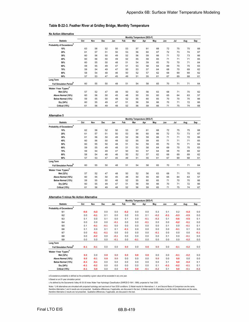
Oct Nov Dec Jan Feb Mar Apr May Jun Jul Aug Sep
10% 63 58 52 50 53 57 61 68 72 75 75 6820% 61 57 51 50 53 56 60 67 72 73 74 6730% 60 56 50 49 52 56 59 66 71 72 73 6640% 60 56 50 49 52 55 59 65 71 71 71 6550% 60 55 50 48 51 54 59 65 70 70 71 6460% 59 55 49 47 51 53 58 64 69 70 70 6370% 59 54 49 47 50 53 57 64 68 70 69 6280% 58 54 48 46 50 52 57 62 68 69 69 6290% 57 53 47 45 49 51 55 61 67 69 68 61
Full Simulation Periodb 60 55 50 48 51 54 58 65 70 71 71 64
Wet (32%) 57 52 47 48 50 52 56 63 68 71 70 62Above Normal (16%) 60 56 50 45 48 50 55 60 65 64 63 57Below Normal (13%) 59 55 50 48 52 55 60 65 70 70 70 66
Dry (24%) 60 55 49 47 51 56 59 66 70 71 72 66Critical (15%) 61 56 49 48 52 56 59 66 71 75 74 68
Oct Nov Dec Jan Feb Mar Apr May Jun Jul Aug Sep
10% 62 58 52 50 53 57 61 68 72 75 75 6820% 61 57 51 50 53 56 60 66 72 73 73 6730% 61 56 50 49 52 56 59 66 71 71 72 6640% 60 56 50 48 52 55 59 65 71 71 71 6550% 60 55 50 48 51 54 59 65 70 70 71 6460% 59 55 49 48 51 53 58 64 69 70 70 6370% 59 54 49 47 50 53 57 64 68 70 69 6280% 58 54 48 46 50 52 57 62 68 69 69 6290% 57 53 47 45 49 51 55 61 67 69 68 61
Full Simulation Periodb 60 55 50 48 51 54 58 65 70 71 71 64
Wet (32%) 57 52 47 48 50 52 56 63 68 71 70 62Above Normal (16%) 60 55 50 45 48 50 55 60 65 64 63 57Below Normal (13%) 59 55 50 48 52 55 60 65 71 70 70 66
Dry (24%) 60 55 49 47 51 56 59 66 70 71 72 66Critical (15%) 61 56 49 48 52 56 59 65 71 75 74 67
Oct Nov Dec Jan Feb Mar Apr May Jun Jul Aug Sep
0.1 -0.6 -0.3 0.0 0.0 -0.2 0.0 0.0 0.3 0.1 0.2 -0.3 0.00.2 0.0 -0.1 0.1 0.0 0.0 0.0 0.1 -0.2 -0.1 -0.3 -0.5 0.00.3 0.1 0.0 0.1 0.0 0.1 0.0 -0.1 -0.2 0.1 -0.6 -0.5 0.10.4 0.0 0.0 0.0 -0.1 0.0 0.0 -0.1 0.0 0.0 -0.2 -0.1 0.00.5 0.1 -0.1 -0.1 0.0 0.0 0.0 0.0 0.0 0.1 0.0 -0.1 0.10.6 0.1 0.0 0.1 0.1 -0.1 0.0 0.0 0.0 0.0 -0.1 0.1 0.00.7 0.0 -0.1 -0.1 0.0 0.0 0.0 0.0 -0.1 0.0 0.0 0.0 -0.1
0.8 0.0 -0.2 0.0 -0.1 0.0 0.0 0.0 0.0 0.1 0.0 -0.1 0.00.9 0.0 0.0 0.0 -0.1 0.0 -0.1 0.0 0.0 0.0 0.0 -0.2 0.0
Full Simulation Periodb
-0.1 -0.1 0.0 0.0 0.0 0.0 0.0 0.0 0.0 -0.1 -0.2 0.0
Wet (32%) 0.0 0.0 0.0 0.0 0.0 0.0 0.0 0.0 0.0 -0.1 -0.2 0.0Above Normal (16%) 0.0 -0.1 0.0 0.0 0.0 0.0 0.0 0.0 0.0 0.0 0.0 0.0Below Normal (13%) -0.1 -0.1 0.0 0.0 0.0 0.0 0.0 0.0 0.1 0.0 -0.4 0.1
Dry (24%) -0.1 -0.2 0.0 0.0 0.0 0.0 0.0 0.1 -0.1 -0.2 -0.1 0.1Critical (15%) -0.1 0.0 0.0 0.0 0.0 0.0 -0.1 -0.2 0.1 0.0 -0.1 -0.2
a Exceedance probability is defined as the probability a given value will be exceeded in any one year.
b Based on an 81-year simulation period.
Probability of Exceedancea
Long Term
Water Year Typesc
c As defined by the Sacramento Valley 40-30-30 Index Water Year Hydrologic Classification (SWRCB D-1641, 1999); projected to Year 2030.
Notes: 1) All alternatives are simulated with projected hydrology and sea level at Year 2030 conditions. 2) Model results for Alternatives 1, 4, and Second Basis of Comparison are the same,
therefore Alternative 1 and 4 results are not presented. Qualitative differences, if applicable, are discussed in the text. 3) Model results for Alternative 2 and No Action Alternative are the same,
therefore Alternative 2 results are not presented. Qualitative differences, if applicable, are discussed in the text.
Probability of Exceedancea
Long Term
Water Year Typesc
Alternative 5 minus No Action Alternative
Statistic
Monthly Temperature (DEG-F)
Long Term
Water Year Typesc
Alternative 5
Statistic
Monthly Temperature (DEG-F)
No Action Alternative
Statistic
Monthly Temperature (DEG-F)
Probability of Exceedancea
Table B-22-3. Feather River at Gridley Bridge, Monthly Temperature
Appendix 6B: Surface Water Temperature Modeling
6B.B-419Final LTO EIS

Oct Nov Dec Jan Feb Mar Apr May Jun Jul Aug Sep
10% 62 58 51 50 53 57 62 67 72 76 75 6920% 62 57 51 50 53 56 60 66 70 75 74 6830% 61 56 50 49 52 56 59 65 70 74 73 6740% 60 55 50 49 52 55 59 65 69 73 72 6650% 60 55 49 48 51 54 59 65 69 72 72 6660% 59 54 49 48 51 53 58 64 68 71 71 6570% 58 53 48 47 50 53 57 63 68 70 71 6580% 58 53 48 46 50 52 57 62 67 70 70 6490% 57 53 47 45 49 51 56 61 66 69 68 64
Full Simulation Periodb 60 55 49 48 51 54 58 64 69 72 72 66
Wet (32%) 57 52 47 48 50 52 56 63 68 71 71 66Above Normal (16%) 61 55 50 45 47 49 54 60 63 64 64 60Below Normal (13%) 59 54 49 48 51 55 60 64 68 71 72 66
Dry (24%) 60 55 49 47 52 56 59 65 69 73 72 66Critical (15%) 61 56 49 48 52 56 59 66 70 76 74 68
Oct Nov Dec Jan Feb Mar Apr May Jun Jul Aug Sep
10% 63 58 52 50 53 57 61 68 72 75 75 6820% 61 57 51 50 53 56 60 67 72 73 74 6730% 60 56 50 49 52 56 59 66 71 72 73 6640% 60 56 50 49 52 55 59 65 71 71 71 6550% 60 55 50 48 51 54 59 65 70 70 71 6460% 59 55 49 47 51 53 58 64 69 70 70 6370% 59 54 49 47 50 53 57 64 68 70 69 6280% 58 54 48 46 50 52 57 62 68 69 69 6290% 57 53 47 45 49 51 55 61 67 69 68 61
Full Simulation Periodb 60 55 50 48 51 54 58 65 70 71 71 64
Wet (32%) 57 52 47 48 50 52 56 63 68 71 70 62Above Normal (16%) 60 56 50 45 48 50 55 60 65 64 63 57Below Normal (13%) 59 55 50 48 52 55 60 65 70 70 70 66
Dry (24%) 60 55 49 47 51 56 59 66 70 71 72 66Critical (15%) 61 56 49 48 52 56 59 66 71 75 74 68
Oct Nov Dec Jan Feb Mar Apr May Jun Jul Aug Sep
0.1 0.7 0.0 0.3 0.1 0.0 0.1 -0.2 1.1 0.5 -0.8 0.2 -0.7
0.2 -0.8 0.0 0.4 0.0 0.0 -0.1 0.0 0.5 1.8 -1.1 -0.2 -0.6
0.3 -0.3 0.2 0.2 -0.2 -0.1 0.2 -0.2 0.5 1.5 -1.6 -0.1 -1.1
0.4 -0.2 0.3 0.3 -0.1 0.1 0.0 0.0 0.4 1.3 -1.7 -1.1 -1.3
0.5 0.1 0.3 0.4 0.1 -0.1 0.2 0.1 0.2 1.1 -1.2 -1.0 -2.1
0.6 0.0 0.7 0.5 -0.1 0.0 0.0 0.0 0.7 1.0 -0.9 -1.0 -2.5
0.7 0.3 0.8 0.4 -0.1 -0.2 0.2 -0.1 0.6 0.9 -0.7 -1.3 -2.3
0.8 0.2 0.9 0.4 0.1 0.1 -0.1 0.0 0.0 1.0 -0.9 -0.9 -2.4
0.9 -0.1 0.0 0.3 0.0 0.0 0.1 -0.1 0.0 0.7 -0.1 -0.3 -2.3
Full Simulation Periodb
0.0 0.3 0.4 -0.1 0.0 0.0 0.0 0.3 1.0 -0.9 -0.6 -1.6
Wet (32%) 0.2 0.5 0.1 -0.2 -0.1 0.0 0.0 0.0 0.3 -0.6 -1.0 -3.9
Above Normal (16%) -0.3 0.2 0.6 0.0 0.2 0.3 0.1 0.5 1.5 -0.4 -0.9 -2.1
Below Normal (13%) 0.0 0.6 0.9 0.0 0.2 0.0 0.0 1.0 2.7 -0.9 -1.6 0.0Dry (24%) -0.1 0.3 0.4 0.0 -0.1 -0.1 -0.1 0.4 1.0 -1.8 0.4 -0.1
Critical (15%) -0.2 -0.5 0.3 0.0 0.1 -0.2 -0.1 0.1 0.4 -0.4 0.2 -0.2
a Exceedance probability is defined as the probability a given value will be exceeded in any one year.
b Based on an 81-year simulation period.
Probability of Exceedancea
Long Term
Water Year Typesc
c As defined by the Sacramento Valley 40-30-30 Index Water Year Hydrologic Classification (SWRCB D-1641, 1999); projected to Year 2030.
Notes: 1) All alternatives are simulated with projected hydrology and sea level at Year 2030 conditions. 2) Model results for Alternatives 1, 4, and Second Basis of Comparison are the same,
therefore Alternative 1 and 4 results are not presented. Qualitative differences, if applicable, are discussed in the text. 3) Model results for Alternative 2 and No Action Alternative are the same,
therefore Alternative 2 results are not presented. Qualitative differences, if applicable, are discussed in the text.
Probability of Exceedancea
Long Term
Water Year Typesc
No Action Alternative minus Second Basis of Comparison
Statistic
Monthly Temperature (DEG-F)
Long Term
Water Year Typesc
No Action Alternative
Statistic
Monthly Temperature (DEG-F)
Second Basis of Comparison
Statistic
Monthly Temperature (DEG-F)
Probability of Exceedancea
Table B-22-4. Feather River at Gridley Bridge, Monthly Temperature
Appendix 6B: Surface Water Temperature Modeling
6B.B-420Final LTO EIS

Oct Nov Dec Jan Feb Mar Apr May Jun Jul Aug Sep
10% 62 58 51 50 53 57 62 67 72 76 75 6920% 62 57 51 50 53 56 60 66 70 75 74 6830% 61 56 50 49 52 56 59 65 70 74 73 6740% 60 55 50 49 52 55 59 65 69 73 72 6650% 60 55 49 48 51 54 59 65 69 72 72 6660% 59 54 49 48 51 53 58 64 68 71 71 6570% 58 53 48 47 50 53 57 63 68 70 71 6580% 58 53 48 46 50 52 57 62 67 70 70 6490% 57 53 47 45 49 51 56 61 66 69 68 64
Full Simulation Periodb 60 55 49 48 51 54 58 64 69 72 72 66
Wet (32%) 57 52 47 48 50 52 56 63 68 71 71 66Above Normal (16%) 61 55 50 45 47 49 54 60 63 64 64 60Below Normal (13%) 59 54 49 48 51 55 60 64 68 71 72 66
Dry (24%) 60 55 49 47 52 56 59 65 69 73 72 66Critical (15%) 61 56 49 48 52 56 59 66 70 76 74 68
Oct Nov Dec Jan Feb Mar Apr May Jun Jul Aug Sep
10% 62 58 51 50 53 57 61 68 71 76 75 6820% 61 57 51 50 53 56 60 66 70 74 74 6830% 61 56 50 49 52 55 59 65 70 72 73 6840% 60 55 50 49 52 55 59 65 70 71 72 6750% 59 54 50 48 51 54 59 65 69 70 71 6660% 59 54 49 47 51 53 58 64 68 70 71 6670% 59 53 48 47 50 53 57 63 68 70 70 6580% 58 53 48 46 50 52 57 62 67 69 69 6490% 57 52 47 45 49 51 55 61 66 68 68 64
Full Simulation Periodb 60 55 49 48 51 54 58 64 69 71 71 66
Wet (32%) 57 52 47 48 50 52 56 63 68 71 71 66Above Normal (16%) 60 55 50 45 48 49 54 60 64 64 64 60Below Normal (13%) 59 54 49 48 51 55 60 65 69 70 70 67
Dry (24%) 60 55 49 47 51 56 59 66 69 72 72 66Critical (15%) 60 56 49 48 52 55 59 66 70 76 74 67
Oct Nov Dec Jan Feb Mar Apr May Jun Jul Aug Sep
0.1 0.1 -0.1 -0.1 0.1 0.1 -0.1 -0.2 1.0 -0.4 0.0 0.3 -0.3
0.2 -0.2 0.0 0.0 0.0 0.1 -0.1 0.0 0.0 0.3 -0.8 -0.1 0.30.3 -0.2 0.0 0.2 -0.1 0.1 -0.2 -0.2 0.0 0.4 -1.9 0.0 0.60.4 -0.3 0.1 0.2 -0.1 0.0 0.0 0.0 0.3 0.2 -1.8 -0.4 0.60.5 -0.2 -0.5 0.1 0.1 0.0 -0.1 0.1 0.0 0.2 -1.2 -0.8 0.10.6 0.1 -0.1 0.2 -0.1 -0.1 0.0 0.0 0.2 0.0 -1.0 -0.6 0.40.7 0.3 0.0 0.1 -0.1 -0.1 0.2 0.0 0.3 0.5 -0.6 -0.7 0.20.8 0.2 0.1 0.2 0.0 0.0 0.0 0.0 0.1 0.0 -0.8 -0.9 -0.2
0.9 -0.1 -0.2 -0.3 0.0 0.0 0.1 -0.1 0.2 0.3 -0.2 -0.3 0.0
Full Simulation Periodb
-0.1 -0.1 0.0 0.0 0.0 -0.1 0.0 0.2 0.1 -0.7 -0.3 0.2
Wet (32%) 0.1 0.1 0.0 0.0 0.0 0.0 0.0 -0.1 -0.3 -0.5 -0.3 0.3Above Normal (16%) -0.3 -0.2 0.2 0.0 0.2 0.1 0.0 0.1 0.6 -0.5 -0.5 0.2Below Normal (13%) 0.1 0.0 -0.1 0.0 0.0 0.0 -0.1 0.6 1.5 -1.3 -2.1 0.8
Dry (24%) 0.1 -0.1 0.1 0.0 -0.1 -0.1 0.0 0.2 -0.2 -1.2 0.5 0.2Critical (15%) -0.5 -0.5 0.2 -0.1 0.1 -0.4 0.0 0.2 -0.2 -0.1 0.1 -0.3
a Exceedance probability is defined as the probability a given value will be exceeded in any one year.
b Based on an 81-year simulation period.
Probability of Exceedancea
Long Term
Water Year Typesc
c As defined by the Sacramento Valley 40-30-30 Index Water Year Hydrologic Classification (SWRCB D-1641, 1999); projected to Year 2030.
Notes: 1) All alternatives are simulated with projected hydrology and sea level at Year 2030 conditions. 2) Model results for Alternatives 1, 4, and Second Basis of Comparison are the same,
therefore Alternative 1 and 4 results are not presented. Qualitative differences, if applicable, are discussed in the text. 3) Model results for Alternative 2 and No Action Alternative are the same,
therefore Alternative 2 results are not presented. Qualitative differences, if applicable, are discussed in the text.
Probability of Exceedancea
Long Term
Water Year Typesc
Alternative 3 minus Second Basis of Comparison
Statistic
Monthly Temperature (DEG-F)
Long Term
Water Year Typesc
Alternative 3
Statistic
Monthly Temperature (DEG-F)
Second Basis of Comparison
Statistic
Monthly Temperature (DEG-F)
Probability of Exceedancea
Table B-22-5. Feather River at Gridley Bridge, Monthly Temperature
Appendix 6B: Surface Water Temperature Modeling
6B.B-421Final LTO EIS
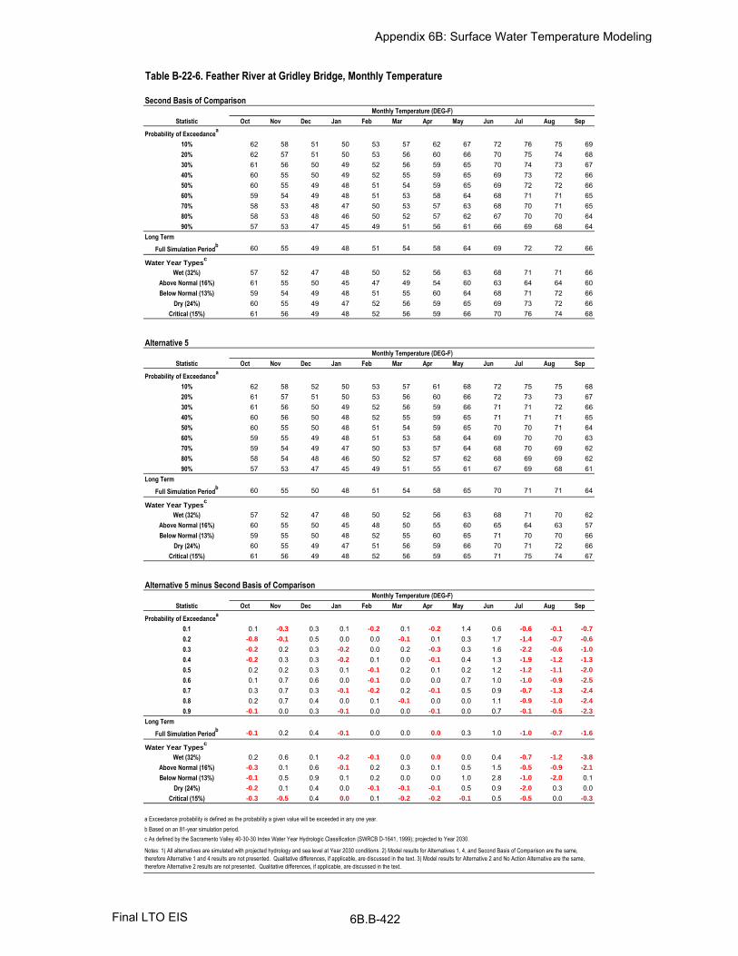
Oct Nov Dec Jan Feb Mar Apr May Jun Jul Aug Sep
10% 62 58 51 50 53 57 62 67 72 76 75 6920% 62 57 51 50 53 56 60 66 70 75 74 6830% 61 56 50 49 52 56 59 65 70 74 73 6740% 60 55 50 49 52 55 59 65 69 73 72 6650% 60 55 49 48 51 54 59 65 69 72 72 6660% 59 54 49 48 51 53 58 64 68 71 71 6570% 58 53 48 47 50 53 57 63 68 70 71 6580% 58 53 48 46 50 52 57 62 67 70 70 6490% 57 53 47 45 49 51 56 61 66 69 68 64
Full Simulation Periodb 60 55 49 48 51 54 58 64 69 72 72 66
Wet (32%) 57 52 47 48 50 52 56 63 68 71 71 66Above Normal (16%) 61 55 50 45 47 49 54 60 63 64 64 60Below Normal (13%) 59 54 49 48 51 55 60 64 68 71 72 66
Dry (24%) 60 55 49 47 52 56 59 65 69 73 72 66Critical (15%) 61 56 49 48 52 56 59 66 70 76 74 68
Oct Nov Dec Jan Feb Mar Apr May Jun Jul Aug Sep
10% 62 58 52 50 53 57 61 68 72 75 75 6820% 61 57 51 50 53 56 60 66 72 73 73 6730% 61 56 50 49 52 56 59 66 71 71 72 6640% 60 56 50 48 52 55 59 65 71 71 71 6550% 60 55 50 48 51 54 59 65 70 70 71 6460% 59 55 49 48 51 53 58 64 69 70 70 6370% 59 54 49 47 50 53 57 64 68 70 69 6280% 58 54 48 46 50 52 57 62 68 69 69 6290% 57 53 47 45 49 51 55 61 67 69 68 61
Full Simulation Periodb 60 55 50 48 51 54 58 65 70 71 71 64
Wet (32%) 57 52 47 48 50 52 56 63 68 71 70 62Above Normal (16%) 60 55 50 45 48 50 55 60 65 64 63 57Below Normal (13%) 59 55 50 48 52 55 60 65 71 70 70 66
Dry (24%) 60 55 49 47 51 56 59 66 70 71 72 66Critical (15%) 61 56 49 48 52 56 59 65 71 75 74 67
Oct Nov Dec Jan Feb Mar Apr May Jun Jul Aug Sep
0.1 0.1 -0.3 0.3 0.1 -0.2 0.1 -0.2 1.4 0.6 -0.6 -0.1 -0.7
0.2 -0.8 -0.1 0.5 0.0 0.0 -0.1 0.1 0.3 1.7 -1.4 -0.7 -0.6
0.3 -0.2 0.2 0.3 -0.2 0.0 0.2 -0.3 0.3 1.6 -2.2 -0.6 -1.0
0.4 -0.2 0.3 0.3 -0.2 0.1 0.0 -0.1 0.4 1.3 -1.9 -1.2 -1.3
0.5 0.2 0.2 0.3 0.1 -0.1 0.2 0.1 0.2 1.2 -1.2 -1.1 -2.0
0.6 0.1 0.7 0.6 0.0 -0.1 0.0 0.0 0.7 1.0 -1.0 -0.9 -2.5
0.7 0.3 0.7 0.3 -0.1 -0.2 0.2 -0.1 0.5 0.9 -0.7 -1.3 -2.4
0.8 0.2 0.7 0.4 0.0 0.1 -0.1 0.0 0.0 1.1 -0.9 -1.0 -2.4
0.9 -0.1 0.0 0.3 -0.1 0.0 0.0 -0.1 0.0 0.7 -0.1 -0.5 -2.3
Full Simulation Periodb
-0.1 0.2 0.4 -0.1 0.0 0.0 0.0 0.3 1.0 -1.0 -0.7 -1.6
Wet (32%) 0.2 0.6 0.1 -0.2 -0.1 0.0 0.0 0.0 0.4 -0.7 -1.2 -3.8
Above Normal (16%) -0.3 0.1 0.6 -0.1 0.2 0.3 0.1 0.5 1.5 -0.5 -0.9 -2.1
Below Normal (13%) -0.1 0.5 0.9 0.1 0.2 0.0 0.0 1.0 2.8 -1.0 -2.0 0.1Dry (24%) -0.2 0.1 0.4 0.0 -0.1 -0.1 -0.1 0.5 0.9 -2.0 0.3 0.0
Critical (15%) -0.3 -0.5 0.4 0.0 0.1 -0.2 -0.2 -0.1 0.5 -0.5 0.0 -0.3
a Exceedance probability is defined as the probability a given value will be exceeded in any one year.
b Based on an 81-year simulation period.
Probability of Exceedancea
Long Term
Water Year Typesc
c As defined by the Sacramento Valley 40-30-30 Index Water Year Hydrologic Classification (SWRCB D-1641, 1999); projected to Year 2030.
Notes: 1) All alternatives are simulated with projected hydrology and sea level at Year 2030 conditions. 2) Model results for Alternatives 1, 4, and Second Basis of Comparison are the same,
therefore Alternative 1 and 4 results are not presented. Qualitative differences, if applicable, are discussed in the text. 3) Model results for Alternative 2 and No Action Alternative are the same,
therefore Alternative 2 results are not presented. Qualitative differences, if applicable, are discussed in the text.
Probability of Exceedancea
Long Term
Water Year Typesc
Alternative 5 minus Second Basis of Comparison
Statistic
Monthly Temperature (DEG-F)
Long Term
Water Year Typesc
Alternative 5
Statistic
Monthly Temperature (DEG-F)
Second Basis of Comparison
Statistic
Monthly Temperature (DEG-F)
Probability of Exceedancea
Table B-22-6. Feather River at Gridley Bridge, Monthly Temperature
Appendix 6B: Surface Water Temperature Modeling
6B.B-422Final LTO EIS

B.23. Feather River at Mouth
Appendix 6B: Surface Water Temperature Modeling
6B.B-423Final LTO EIS

Figure B-23-1. Feather River at Mouth, October
Notes: 1) Exceedance probability is defined as the probability a given value will be exceeded in any one year. 2) All alternatives are simulated with projected hydrology and
sea level at Year 2030 conditions. 3) Model results for Alternatives 1, 4, and Second Basis of Comparison are the same, therefore Alternatives 1 and 4 results are not
presented. Qualitative differences, if applicable, are discussed in the text. 4) Model results for Alternative 2 and No Action Alternative are the same, therefore Alternative 2
results are not presented. Qualitative differences, if applicable, are discussed in the text.
44464850525456586062646668707274767880828486
0%10%20%30%40%50%60%70%80%90%100%
Exceedance Probability
No Action Alternative & Alternative 2 Second Basis of Comparison, Alternative 1, & Alternative 4
Alternative 3 Alternative 5
Mon
thly
Tem
pera
ture
(DE
G-F
)
Appendix 6B: Surface Water Temperature Modeling
6B.B-424Final LTO EIS

Figure B-23-2. Feather River at Mouth, November
Notes: 1) Exceedance probability is defined as the probability a given value will be exceeded in any one year. 2) All alternatives are simulated with projected hydrology and
sea level at Year 2030 conditions. 3) Model results for Alternatives 1, 4, and Second Basis of Comparison are the same, therefore Alternatives 1 and 4 results are not
presented. Qualitative differences, if applicable, are discussed in the text. 4) Model results for Alternative 2 and No Action Alternative are the same, therefore Alternative 2
results are not presented. Qualitative differences, if applicable, are discussed in the text.
44464850525456586062646668707274767880828486
0%10%20%30%40%50%60%70%80%90%100%
Exceedance Probability
No Action Alternative & Alternative 2 Second Basis of Comparison, Alternative 1, & Alternative 4
Alternative 3 Alternative 5
Mon
thly
Tem
pera
ture
(DE
G-F
)
Appendix 6B: Surface Water Temperature Modeling
6B.B-245Final LTO EIS

Figure B-23-3. Feather River at Mouth, December
Notes: 1) Exceedance probability is defined as the probability a given value will be exceeded in any one year. 2) All alternatives are simulated with projected hydrology and
sea level at Year 2030 conditions. 3) Model results for Alternatives 1, 4, and Second Basis of Comparison are the same, therefore Alternatives 1 and 4 results are not
presented. Qualitative differences, if applicable, are discussed in the text. 4) Model results for Alternative 2 and No Action Alternative are the same, therefore Alternative 2
results are not presented. Qualitative differences, if applicable, are discussed in the text.
44464850525456586062646668707274767880828486
0%10%20%30%40%50%60%70%80%90%100%
Exceedance Probability
No Action Alternative & Alternative 2 Second Basis of Comparison, Alternative 1, & Alternative 4
Alternative 3 Alternative 5
Mon
thly
Tem
pera
ture
(DE
G-F
)
Appendix 6B: Surface Water Temperature Modeling
6B.B-426Final LTO EIS

Figure B-23-4. Feather River at Mouth, January
Notes: 1) Exceedance probability is defined as the probability a given value will be exceeded in any one year. 2) All alternatives are simulated with projected hydrology and
sea level at Year 2030 conditions. 3) Model results for Alternatives 1, 4, and Second Basis of Comparison are the same, therefore Alternatives 1 and 4 results are not
presented. Qualitative differences, if applicable, are discussed in the text. 4) Model results for Alternative 2 and No Action Alternative are the same, therefore Alternative 2
results are not presented. Qualitative differences, if applicable, are discussed in the text.
44464850525456586062646668707274767880828486
0%10%20%30%40%50%60%70%80%90%100%
Exceedance Probability
No Action Alternative & Alternative 2 Second Basis of Comparison, Alternative 1, & Alternative 4
Alternative 3 Alternative 5
Mon
thly
Tem
pera
ture
(DE
G-F
)
Appendix 6B: Surface Water Temperature Modeling
6B.B-427Final LTO EIS

Figure B-23-5. Feather River at Mouth, February
Notes: 1) Exceedance probability is defined as the probability a given value will be exceeded in any one year. 2) All alternatives are simulated with projected hydrology and
sea level at Year 2030 conditions. 3) Model results for Alternatives 1, 4, and Second Basis of Comparison are the same, therefore Alternatives 1 and 4 results are not
presented. Qualitative differences, if applicable, are discussed in the text. 4) Model results for Alternative 2 and No Action Alternative are the same, therefore Alternative 2
results are not presented. Qualitative differences, if applicable, are discussed in the text.
44464850525456586062646668707274767880828486
0%10%20%30%40%50%60%70%80%90%100%
Exceedance Probability
No Action Alternative & Alternative 2 Second Basis of Comparison, Alternative 1, & Alternative 4
Alternative 3 Alternative 5
Mon
thly
Tem
pera
ture
(DE
G-F
)
Appendix 6B: Surface Water Temperature Modeling
6B.B-428Final LTO EIS

Figure B-23-6. Feather River at Mouth, March
Notes: 1) Exceedance probability is defined as the probability a given value will be exceeded in any one year. 2) All alternatives are simulated with projected hydrology and
sea level at Year 2030 conditions. 3) Model results for Alternatives 1, 4, and Second Basis of Comparison are the same, therefore Alternatives 1 and 4 results are not
presented. Qualitative differences, if applicable, are discussed in the text. 4) Model results for Alternative 2 and No Action Alternative are the same, therefore Alternative 2
results are not presented. Qualitative differences, if applicable, are discussed in the text.
44464850525456586062646668707274767880828486
0%10%20%30%40%50%60%70%80%90%100%
Exceedance Probability
No Action Alternative & Alternative 2 Second Basis of Comparison, Alternative 1, & Alternative 4
Alternative 3 Alternative 5
Mon
thly
Tem
pera
ture
(DE
G-F
)
Appendix 6B: Surface Water Temperature Modeling
6B.B-429Final LTO EIS

Figure B-23-7. Feather River at Mouth, April
Notes: 1) Exceedance probability is defined as the probability a given value will be exceeded in any one year. 2) All alternatives are simulated with projected hydrology and
sea level at Year 2030 conditions. 3) Model results for Alternatives 1, 4, and Second Basis of Comparison are the same, therefore Alternatives 1 and 4 results are not
presented. Qualitative differences, if applicable, are discussed in the text. 4) Model results for Alternative 2 and No Action Alternative are the same, therefore Alternative 2
results are not presented. Qualitative differences, if applicable, are discussed in the text.
44464850525456586062646668707274767880828486
0%10%20%30%40%50%60%70%80%90%100%
Exceedance Probability
No Action Alternative & Alternative 2 Second Basis of Comparison, Alternative 1, & Alternative 4
Alternative 3 Alternative 5
Mon
thly
Tem
pera
ture
(DE
G-F
)
Appendix 6B: Surface Water Temperature Modeling
6B.B-430Final LTO EIS

Figure B-23-8. Feather River at Mouth, May
Notes: 1) Exceedance probability is defined as the probability a given value will be exceeded in any one year. 2) All alternatives are simulated with projected hydrology and
sea level at Year 2030 conditions. 3) Model results for Alternatives 1, 4, and Second Basis of Comparison are the same, therefore Alternatives 1 and 4 results are not
presented. Qualitative differences, if applicable, are discussed in the text. 4) Model results for Alternative 2 and No Action Alternative are the same, therefore Alternative 2
results are not presented. Qualitative differences, if applicable, are discussed in the text.
44464850525456586062646668707274767880828486
0%10%20%30%40%50%60%70%80%90%100%
Exceedance Probability
No Action Alternative & Alternative 2 Second Basis of Comparison, Alternative 1, & Alternative 4
Alternative 3 Alternative 5
Mon
thly
Tem
pera
ture
(DE
G-F
)
Appendix 6B: Surface Water Temperature Modeling
6B.B-431Final LTO EIS

Figure B-23-9. Feather River at Mouth, June
Notes: 1) Exceedance probability is defined as the probability a given value will be exceeded in any one year. 2) All alternatives are simulated with projected hydrology and
sea level at Year 2030 conditions. 3) Model results for Alternatives 1, 4, and Second Basis of Comparison are the same, therefore Alternatives 1 and 4 results are not
presented. Qualitative differences, if applicable, are discussed in the text. 4) Model results for Alternative 2 and No Action Alternative are the same, therefore Alternative 2
results are not presented. Qualitative differences, if applicable, are discussed in the text.
44464850525456586062646668707274767880828486
0%10%20%30%40%50%60%70%80%90%100%
Exceedance Probability
No Action Alternative & Alternative 2 Second Basis of Comparison, Alternative 1, & Alternative 4
Alternative 3 Alternative 5
Mon
thly
Tem
pera
ture
(DE
G-F
)
Appendix 6B: Surface Water Temperature Modeling
6B.B-432Final LTO EIS

Figure B-23-10. Feather River at Mouth, July
Notes: 1) Exceedance probability is defined as the probability a given value will be exceeded in any one year. 2) All alternatives are simulated with projected hydrology and
sea level at Year 2030 conditions. 3) Model results for Alternatives 1, 4, and Second Basis of Comparison are the same, therefore Alternatives 1 and 4 results are not
presented. Qualitative differences, if applicable, are discussed in the text. 4) Model results for Alternative 2 and No Action Alternative are the same, therefore Alternative 2
results are not presented. Qualitative differences, if applicable, are discussed in the text.
44464850525456586062646668707274767880828486
0%10%20%30%40%50%60%70%80%90%100%
Exceedance Probability
No Action Alternative & Alternative 2 Second Basis of Comparison, Alternative 1, & Alternative 4
Alternative 3 Alternative 5
Mon
thly
Tem
pera
ture
(DE
G-F
)
Appendix 6B: Surface Water Temperature Modeling
6B.B-433Final LTO EIS

Figure B-23-11. Feather River at Mouth, August
Notes: 1) Exceedance probability is defined as the probability a given value will be exceeded in any one year. 2) All alternatives are simulated with projected hydrology and
sea level at Year 2030 conditions. 3) Model results for Alternatives 1, 4, and Second Basis of Comparison are the same, therefore Alternatives 1 and 4 results are not
presented. Qualitative differences, if applicable, are discussed in the text. 4) Model results for Alternative 2 and No Action Alternative are the same, therefore Alternative 2
results are not presented. Qualitative differences, if applicable, are discussed in the text.
44464850525456586062646668707274767880828486
0%10%20%30%40%50%60%70%80%90%100%
Exceedance Probability
No Action Alternative & Alternative 2 Second Basis of Comparison, Alternative 1, & Alternative 4
Alternative 3 Alternative 5
Mon
thly
Tem
pera
ture
(DE
G-F
)
Appendix 6B: Surface Water Temperature Modeling
6B.B-434Final LTO EIS

Figure B-23-12. Feather River at Mouth, September
Notes: 1) Exceedance probability is defined as the probability a given value will be exceeded in any one year. 2) All alternatives are simulated with projected hydrology and
sea level at Year 2030 conditions. 3) Model results for Alternatives 1, 4, and Second Basis of Comparison are the same, therefore Alternatives 1 and 4 results are not
presented. Qualitative differences, if applicable, are discussed in the text. 4) Model results for Alternative 2 and No Action Alternative are the same, therefore Alternative 2
results are not presented. Qualitative differences, if applicable, are discussed in the text.
44464850525456586062646668707274767880828486
0%10%20%30%40%50%60%70%80%90%100%
Exceedance Probability
No Action Alternative & Alternative 2 Second Basis of Comparison, Alternative 1, & Alternative 4
Alternative 3 Alternative 5
Mon
thly
Tem
pera
ture
(DE
G-F
)
Appendix 6B: Surface Water Temperature Modeling
6B.B-435Final LTO EIS
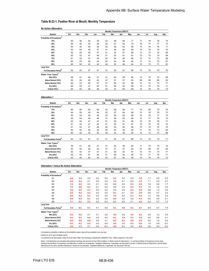
Oct Nov Dec Jan Feb Mar Apr May Jun Jul Aug Sep
10% 65 56 50 49 53 58 66 71 77 78 78 7420% 64 55 49 48 52 57 63 70 76 77 77 7330% 63 55 48 48 52 56 63 69 75 76 76 7140% 63 54 48 47 51 56 62 69 74 76 75 7050% 62 54 48 47 51 55 61 68 73 75 74 6960% 62 53 47 46 51 55 61 67 73 75 74 6870% 61 53 47 46 50 54 60 66 72 74 73 6880% 60 53 46 45 50 54 58 65 71 73 72 6790% 60 52 45 45 49 53 58 64 70 73 71 67
Full Simulation Periodb 62 54 47 47 51 55 61 68 73 75 75 70
Wet (32%) 59 51 46 47 51 54 59 66 72 75 74 68Above Normal (16%) 62 54 48 44 47 51 57 63 68 68 66 62Below Normal (13%) 62 53 48 47 51 56 63 68 74 74 74 71
Dry (24%) 62 54 47 46 51 56 62 69 74 75 76 71Critical (15%) 64 54 46 46 52 57 64 69 74 79 78 72
Oct Nov Dec Jan Feb Mar Apr May Jun Jul Aug Sep
10% 65 56 50 49 53 58 66 71 75 80 79 7420% 64 55 49 48 52 57 64 69 74 78 78 7330% 63 54 48 48 52 56 63 69 74 78 77 7340% 63 54 48 48 51 56 62 68 73 77 76 7250% 62 54 47 47 51 55 61 68 73 76 76 7160% 61 53 47 46 51 55 61 67 72 75 75 7070% 61 53 47 46 50 54 60 66 72 75 74 7080% 60 52 46 45 50 54 58 65 71 74 73 6990% 60 52 45 45 49 53 58 65 70 73 72 68
Full Simulation Periodb 62 54 47 47 51 55 61 68 73 76 75 71
Wet (32%) 59 51 46 47 51 54 59 66 71 75 75 72Above Normal (16%) 62 54 48 44 47 51 57 62 67 68 67 64Below Normal (13%) 62 53 47 47 51 56 62 67 72 75 75 71
Dry (24%) 62 54 47 46 51 56 62 69 74 77 76 71Critical (15%) 63 55 46 46 52 57 64 69 74 79 78 72
Oct Nov Dec Jan Feb Mar Apr May Jun Jul Aug Sep
0.1 -0.2 0.0 0.0 0.0 0.0 -0.1 0.0 0.0 -1.2 1.7 0.4 0.30.2 -0.1 -0.1 0.1 0.0 0.0 0.0 0.1 -0.4 -1.3 1.1 0.3 0.70.3 0.2 -0.2 0.0 0.1 0.0 -0.2 0.0 -0.3 -0.9 1.8 0.8 1.70.4 0.0 -0.3 -0.1 0.1 0.0 0.0 0.0 -0.4 -0.7 1.4 1.0 2.20.5 -0.2 -0.2 -0.1 0.0 0.0 0.0 0.0 -0.3 -0.9 0.8 1.3 2.00.6 -0.2 -0.2 -0.3 0.0 0.0 -0.1 0.1 -0.5 -0.9 0.8 0.7 2.30.7 -0.4 -0.1 -0.1 0.0 0.0 0.0 0.0 -0.1 -0.4 1.2 0.8 2.20.8 -0.3 -0.3 -0.1 0.0 0.0 -0.2 0.0 0.0 -0.3 0.6 0.9 2.10.9 0.1 -0.1 0.3 0.0 -0.1 -0.1 0.0 0.1 -0.3 0.4 0.7 1.7
Full Simulation Periodb
-0.2 -0.1 -0.1 0.1 0.0 -0.1 0.0 -0.2 -0.7 0.9 0.7 1.6
Wet (32%) -0.1 -0.2 0.1 0.1 0.0 0.0 0.0 0.0 -0.2 0.6 1.2 4.0Above Normal (16%) -0.1 -0.1 -0.4 0.0 0.0 -0.1 0.0 -0.3 -0.9 0.5 0.8 2.1Below Normal (13%) -0.1 -0.3 -0.6 0.0 0.1 -0.1 -0.1 -0.8 -2.0 0.9 1.5 0.2
Dry (24%) -0.1 -0.1 -0.2 0.0 0.0 0.0 0.0 -0.3 -0.6 1.6 0.0 -0.1
Critical (15%) -0.5 0.3 0.1 0.0 -0.1 0.0 -0.1 0.0 -0.5 0.6 0.0 -0.1
a Exceedance probability is defined as the probability a given value will be exceeded in any one year.
b Based on an 81-year simulation period.
Probability of Exceedancea
Long Term
Water Year Typesc
c As defined by the Sacramento Valley 40-30-30 Index Water Year Hydrologic Classification (SWRCB D-1641, 1999); projected to Year 2030.
Notes: 1) All alternatives are simulated with projected hydrology and sea level at Year 2030 conditions. 2) Model results for Alternatives 1, 4, and Second Basis of Comparison are the same,
therefore Second Basis of Comparison and Alternative 4 results are not presented. Qualitative differences, if applicable, are discussed in the text. 3) Model results for Alternative 2 and No Action
Alternative are the same, therefore Alternative 2 results are not presented. Qualitative differences, if applicable, are discussed in the text.
Probability of Exceedancea
Long Term
Water Year Typesc
Alternative 1 minus No Action Alternative
Statistic
Monthly Temperature (DEG-F)
Long Term
Water Year Typesc
Alternative 1
Statistic
Monthly Temperature (DEG-F)
No Action Alternative
Statistic
Monthly Temperature (DEG-F)
Probability of Exceedancea
Table B-23-1. Feather River at Mouth, Monthly Temperature
Appendix 6B: Surface Water Temperature Modeling
6B.B-436Final LTO EIS

Oct Nov Dec Jan Feb Mar Apr May Jun Jul Aug Sep
10% 65 56 50 49 53 58 66 71 77 78 78 7420% 64 55 49 48 52 57 63 70 76 77 77 7330% 63 55 48 48 52 56 63 69 75 76 76 7140% 63 54 48 47 51 56 62 69 74 76 75 7050% 62 54 48 47 51 55 61 68 73 75 74 6960% 62 53 47 46 51 55 61 67 73 75 74 6870% 61 53 47 46 50 54 60 66 72 74 73 6880% 60 53 46 45 50 54 58 65 71 73 72 6790% 60 52 45 45 49 53 58 64 70 73 71 67
Full Simulation Periodb 62 54 47 47 51 55 61 68 73 75 75 70
Wet (32%) 59 51 46 47 51 54 59 66 72 75 74 68Above Normal (16%) 62 54 48 44 47 51 57 63 68 68 66 62Below Normal (13%) 62 53 48 47 51 56 63 68 74 74 74 71
Dry (24%) 62 54 47 46 51 56 62 69 74 75 76 71Critical (15%) 64 54 46 46 52 57 64 69 74 79 78 72
Oct Nov Dec Jan Feb Mar Apr May Jun Jul Aug Sep
10% 65 55 49 49 53 58 65 71 75 79 79 7420% 64 55 49 48 52 57 63 70 75 77 78 7430% 63 54 48 48 52 56 63 69 74 76 77 7340% 63 54 48 47 51 56 62 68 73 76 76 7250% 62 54 48 47 51 55 61 68 73 75 75 7160% 61 53 47 47 51 55 61 67 72 75 74 7170% 61 53 47 46 50 54 60 66 72 74 73 7080% 60 52 46 45 50 54 58 65 71 73 72 6990% 60 52 45 45 49 53 58 65 70 73 72 69
Full Simulation Periodb 62 54 47 47 51 55 61 68 73 76 75 71
Wet (32%) 59 51 46 47 51 54 59 66 71 75 75 72Above Normal (16%) 62 54 48 44 47 51 57 62 67 68 67 64Below Normal (13%) 62 53 47 47 51 56 62 68 73 74 73 71
Dry (24%) 62 54 47 46 51 56 62 69 74 76 76 72Critical (15%) 63 54 46 46 52 57 64 69 74 79 78 72
Oct Nov Dec Jan Feb Mar Apr May Jun Jul Aug Sep
0.1 0.0 -0.3 -0.2 0.0 0.0 -0.1 -0.3 0.1 -1.2 1.0 0.5 0.30.2 0.1 -0.1 0.0 0.0 0.0 -0.1 0.0 -0.2 -1.0 0.3 0.3 0.90.3 0.2 -0.3 -0.1 0.1 0.0 -0.1 0.0 -0.1 -0.9 -0.1 1.2 1.70.4 -0.1 -0.4 -0.1 0.0 0.0 -0.1 0.0 -0.4 -0.6 0.1 0.8 2.30.5 -0.1 -0.3 0.0 0.0 0.0 0.0 0.0 -0.3 -0.5 0.1 0.4 2.10.6 -0.2 -0.3 -0.2 0.1 0.0 0.0 0.0 -0.4 -0.7 0.0 0.4 2.70.7 0.1 -0.1 -0.1 0.0 0.0 0.0 0.0 -0.2 -0.2 0.1 0.2 2.60.8 -0.1 -0.3 -0.1 0.0 0.0 -0.1 0.0 0.0 0.0 0.1 0.2 2.10.9 0.2 -0.2 0.3 0.0 -0.1 -0.1 0.0 0.1 -0.3 0.0 0.2 2.1
Full Simulation Periodb 0.0 -0.2 -0.1 0.0 0.0 0.0 0.0 -0.2 -0.6 0.2 0.4 1.8
Wet (32%) 0.0 -0.2 0.1 0.1 0.0 0.0 0.0 0.0 -0.4 0.2 1.0 4.4Above Normal (16%) -0.1 -0.2 -0.3 0.0 0.0 0.0 0.0 -0.3 -0.5 0.0 0.4 2.1Below Normal (13%) 0.1 -0.3 -0.6 0.0 0.1 0.0 -0.1 -0.4 -0.8 -0.3 -0.2 0.5
Dry (24%) 0.2 -0.2 -0.2 0.0 0.0 -0.1 0.0 -0.2 -0.8 0.5 0.3 0.1Critical (15%) -0.2 0.0 0.2 0.0 0.0 -0.1 0.0 0.0 -0.7 0.3 0.0 0.0
a Exceedance probability is defined as the probability a given value will be exceeded in any one year.
b Based on an 81-year simulation period.
Probability of Exceedancea
Long Term
Water Year Typesc
c As defined by the Sacramento Valley 40-30-30 Index Water Year Hydrologic Classification (SWRCB D-1641, 1999); projected to Year 2030.
Notes: 1) All alternatives are simulated with projected hydrology and sea level at Year 2030 conditions. 2) Model results for Alternatives 1, 4, and Second Basis of Comparison are the same,
therefore Alternative 1 and 4 results are not presented. Qualitative differences, if applicable, are discussed in the text. 3) Model results for Alternative 2 and No Action Alternative are the same,
therefore Alternative 2 results are not presented. Qualitative differences, if applicable, are discussed in the text.
Probability of Exceedancea
Long Term
Water Year Typesc
Alternative 3 minus No Action Alternative
Statistic
Monthly Temperature (DEG-F)
Long Term
Water Year Typesc
Alternative 3
Statistic
Monthly Temperature (DEG-F)
No Action Alternative
Statistic
Monthly Temperature (DEG-F)
Probability of Exceedancea
Table B-23-2. Feather River at Mouth, Monthly Temperature
Appendix 6B: Surface Water Temperature Modeling
6B.B-437Final LTO EIS

Oct Nov Dec Jan Feb Mar Apr May Jun Jul Aug Sep
10% 65 56 50 49 53 58 66 71 77 78 78 7420% 64 55 49 48 52 57 63 70 76 77 77 7330% 63 55 48 48 52 56 63 69 75 76 76 7140% 63 54 48 47 51 56 62 69 74 76 75 7050% 62 54 48 47 51 55 61 68 73 75 74 6960% 62 53 47 46 51 55 61 67 73 75 74 6870% 61 53 47 46 50 54 60 66 72 74 73 6880% 60 53 46 45 50 54 58 65 71 73 72 6790% 60 52 45 45 49 53 58 64 70 73 71 67
Full Simulation Periodb 62 54 47 47 51 55 61 68 73 75 75 70
Wet (32%) 59 51 46 47 51 54 59 66 72 75 74 68Above Normal (16%) 62 54 48 44 47 51 57 63 68 68 66 62Below Normal (13%) 62 53 48 47 51 56 63 68 74 74 74 71
Dry (24%) 62 54 47 46 51 56 62 69 74 75 76 71Critical (15%) 64 54 46 46 52 57 64 69 74 79 78 72
Oct Nov Dec Jan Feb Mar Apr May Jun Jul Aug Sep
10% 65 56 50 49 53 58 66 71 77 78 78 7320% 64 55 49 48 52 57 63 70 76 77 77 7330% 63 55 48 48 52 56 63 69 75 76 76 7140% 63 54 48 47 51 56 62 69 74 75 75 7050% 62 54 48 47 51 55 61 68 73 75 74 6960% 62 53 47 46 51 55 61 68 73 74 74 6970% 61 53 47 46 50 54 60 66 72 74 73 6880% 60 53 46 45 50 54 58 65 71 73 72 6790% 60 52 45 45 49 53 58 64 70 73 71 67
Full Simulation Periodb 62 54 47 47 51 55 61 68 73 75 74 70
Wet (32%) 59 51 46 47 51 54 59 66 72 75 74 68Above Normal (16%) 62 54 48 44 47 51 57 63 68 68 66 62Below Normal (13%) 62 53 48 47 51 56 63 68 74 74 73 70
Dry (24%) 62 54 47 46 51 56 62 70 74 75 75 71Critical (15%) 64 54 46 46 52 57 64 69 74 79 77 72
Oct Nov Dec Jan Feb Mar Apr May Jun Jul Aug Sep
0.1 0.0 0.0 0.0 0.0 0.0 0.0 0.0 0.3 -0.1 0.0 0.0 -0.1
0.2 0.0 0.0 0.0 0.0 0.0 0.0 0.0 0.3 0.0 -0.1 0.0 0.00.3 0.1 0.1 0.0 0.0 0.0 0.0 0.0 0.1 0.0 -0.1 -0.2 0.00.4 0.0 0.0 0.0 0.0 0.0 0.0 0.0 0.1 0.2 -0.1 -0.4 -0.1
0.5 0.0 -0.1 0.1 0.0 0.0 0.0 0.0 0.1 -0.1 0.0 0.0 -0.1
0.6 0.1 0.0 -0.1 0.0 0.0 0.0 0.0 0.2 -0.1 -0.1 -0.2 0.50.7 0.1 0.0 0.0 0.0 0.0 0.0 0.0 0.0 0.2 0.0 -0.1 0.00.8 -0.1 0.1 0.0 0.0 0.0 0.0 0.0 0.0 0.1 0.0 0.0 0.00.9 0.0 0.0 0.8 0.0 0.0 -0.1 0.0 0.0 0.1 0.0 0.0 0.0
Full Simulation Periodb
0.0 0.0 0.0 0.0 0.0 0.0 0.0 0.1 0.0 -0.1 -0.1 0.0
Wet (32%) 0.0 0.0 0.0 0.0 0.0 0.0 0.0 0.0 0.0 0.0 -0.1 0.1Above Normal (16%) 0.0 0.0 0.0 0.0 0.0 0.0 0.0 0.0 0.0 0.0 0.0 0.0Below Normal (13%) 0.0 0.0 0.0 0.0 0.0 0.0 0.0 0.1 0.1 0.0 -0.2 -0.1
Dry (24%) 0.0 0.0 0.0 0.0 0.0 0.0 0.0 0.3 0.0 -0.2 -0.1 0.0
Critical (15%) 0.0 0.0 0.3 0.0 0.0 0.0 0.0 0.1 0.0 -0.1 -0.2 -0.1
a Exceedance probability is defined as the probability a given value will be exceeded in any one year.
b Based on an 81-year simulation period.
Probability of Exceedancea
Long Term
Water Year Typesc
c As defined by the Sacramento Valley 40-30-30 Index Water Year Hydrologic Classification (SWRCB D-1641, 1999); projected to Year 2030.
Notes: 1) All alternatives are simulated with projected hydrology and sea level at Year 2030 conditions. 2) Model results for Alternatives 1, 4, and Second Basis of Comparison are the same,
therefore Alternative 1 and 4 results are not presented. Qualitative differences, if applicable, are discussed in the text. 3) Model results for Alternative 2 and No Action Alternative are the same,
therefore Alternative 2 results are not presented. Qualitative differences, if applicable, are discussed in the text.
Probability of Exceedancea
Long Term
Water Year Typesc
Alternative 5 minus No Action Alternative
Statistic
Monthly Temperature (DEG-F)
Long Term
Water Year Typesc
Alternative 5
Statistic
Monthly Temperature (DEG-F)
No Action Alternative
Statistic
Monthly Temperature (DEG-F)
Probability of Exceedancea
Table B-23-3. Feather River at Mouth, Monthly Temperature
Appendix 6B: Surface Water Temperature Modeling
6B.B-438Final LTO EIS

Oct Nov Dec Jan Feb Mar Apr May Jun Jul Aug Sep
10% 65 56 50 49 53 58 66 71 75 80 79 7420% 64 55 49 48 52 57 64 69 74 78 78 7330% 63 54 48 48 52 56 63 69 74 78 77 7340% 63 54 48 48 51 56 62 68 73 77 76 7250% 62 54 47 47 51 55 61 68 73 76 76 7160% 61 53 47 46 51 55 61 67 72 75 75 7070% 61 53 47 46 50 54 60 66 72 75 74 7080% 60 52 46 45 50 54 58 65 71 74 73 6990% 60 52 45 45 49 53 58 65 70 73 72 68
Full Simulation Periodb 62 54 47 47 51 55 61 68 73 76 75 71
Wet (32%) 59 51 46 47 51 54 59 66 71 75 75 72Above Normal (16%) 62 54 48 44 47 51 57 62 67 68 67 64Below Normal (13%) 62 53 47 47 51 56 62 67 72 75 75 71
Dry (24%) 62 54 47 46 51 56 62 69 74 77 76 71Critical (15%) 63 55 46 46 52 57 64 69 74 79 78 72
Oct Nov Dec Jan Feb Mar Apr May Jun Jul Aug Sep
10% 65 56 50 49 53 58 66 71 77 78 78 7420% 64 55 49 48 52 57 63 70 76 77 77 7330% 63 55 48 48 52 56 63 69 75 76 76 7140% 63 54 48 47 51 56 62 69 74 76 75 7050% 62 54 48 47 51 55 61 68 73 75 74 6960% 62 53 47 46 51 55 61 67 73 75 74 6870% 61 53 47 46 50 54 60 66 72 74 73 6880% 60 53 46 45 50 54 58 65 71 73 72 6790% 60 52 45 45 49 53 58 64 70 73 71 67
Full Simulation Periodb 62 54 47 47 51 55 61 68 73 75 75 70
Wet (32%) 59 51 46 47 51 54 59 66 72 75 74 68Above Normal (16%) 62 54 48 44 47 51 57 63 68 68 66 62Below Normal (13%) 62 53 48 47 51 56 63 68 74 74 74 71
Dry (24%) 62 54 47 46 51 56 62 69 74 75 76 71Critical (15%) 64 54 46 46 52 57 64 69 74 79 78 72
Oct Nov Dec Jan Feb Mar Apr May Jun Jul Aug Sep
0.1 0.2 0.0 0.0 0.0 0.0 0.1 0.0 0.0 1.2 -1.7 -0.4 -0.3
0.2 0.1 0.1 -0.1 0.0 0.0 0.0 -0.1 0.4 1.3 -1.1 -0.3 -0.7
0.3 -0.2 0.2 0.0 -0.1 0.0 0.2 0.0 0.3 0.9 -1.8 -0.8 -1.7
0.4 0.0 0.3 0.1 -0.1 0.0 0.0 0.0 0.4 0.7 -1.4 -1.0 -2.2
0.5 0.2 0.2 0.1 0.0 0.0 0.0 0.0 0.3 0.9 -0.8 -1.3 -2.0
0.6 0.2 0.2 0.3 0.0 0.0 0.1 -0.1 0.5 0.9 -0.8 -0.7 -2.3
0.7 0.4 0.1 0.1 0.0 0.0 0.0 0.0 0.1 0.4 -1.2 -0.8 -2.2
0.8 0.3 0.3 0.1 0.0 0.0 0.2 0.0 0.0 0.3 -0.6 -0.9 -2.1
0.9 -0.1 0.1 -0.3 0.0 0.1 0.1 0.0 -0.1 0.3 -0.4 -0.7 -1.7
Full Simulation Periodb 0.2 0.1 0.1 -0.1 0.0 0.1 0.0 0.2 0.7 -0.9 -0.7 -1.6
Wet (32%) 0.1 0.2 -0.1 -0.1 0.0 0.0 0.0 0.0 0.2 -0.6 -1.2 -4.0
Above Normal (16%) 0.1 0.1 0.4 0.0 0.0 0.1 0.0 0.3 0.9 -0.5 -0.8 -2.1
Below Normal (13%) 0.1 0.3 0.6 0.0 -0.1 0.1 0.1 0.8 2.0 -0.9 -1.5 -0.2
Dry (24%) 0.1 0.1 0.2 0.0 0.0 0.0 0.0 0.3 0.6 -1.6 0.0 0.1Critical (15%) 0.5 -0.3 -0.1 0.0 0.1 0.0 0.1 0.0 0.5 -0.6 0.0 0.1
a Exceedance probability is defined as the probability a given value will be exceeded in any one year.
b Based on an 81-year simulation period.
Probability of Exceedancea
Long Term
Water Year Typesc
c As defined by the Sacramento Valley 40-30-30 Index Water Year Hydrologic Classification (SWRCB D-1641, 1999); projected to Year 2030.
Notes: 1) All alternatives are simulated with projected hydrology and sea level at Year 2030 conditions. 2) Model results for Alternatives 1, 4, and Second Basis of Comparison are the same,
therefore Alternative 1 and 4 results are not presented. Qualitative differences, if applicable, are discussed in the text. 3) Model results for Alternative 2 and No Action Alternative are the same,
therefore Alternative 2 results are not presented. Qualitative differences, if applicable, are discussed in the text.
Probability of Exceedancea
Long Term
Water Year Typesc
No Action Alternative minus Second Basis of Comparison
Statistic
Monthly Temperature (DEG-F)
Long Term
Water Year Typesc
No Action Alternative
Statistic
Monthly Temperature (DEG-F)
Second Basis of Comparison
Statistic
Monthly Temperature (DEG-F)
Probability of Exceedancea
Table B-23-4. Feather River at Mouth, Monthly Temperature
Appendix 6B: Surface Water Temperature Modeling
6B.B-439Final LTO EIS

Oct Nov Dec Jan Feb Mar Apr May Jun Jul Aug Sep
10% 65 56 50 49 53 58 66 71 75 80 79 7420% 64 55 49 48 52 57 64 69 74 78 78 7330% 63 54 48 48 52 56 63 69 74 78 77 7340% 63 54 48 48 51 56 62 68 73 77 76 7250% 62 54 47 47 51 55 61 68 73 76 76 7160% 61 53 47 46 51 55 61 67 72 75 75 7070% 61 53 47 46 50 54 60 66 72 75 74 7080% 60 52 46 45 50 54 58 65 71 74 73 6990% 60 52 45 45 49 53 58 65 70 73 72 68
Full Simulation Periodb 62 54 47 47 51 55 61 68 73 76 75 71
Wet (32%) 59 51 46 47 51 54 59 66 71 75 75 72Above Normal (16%) 62 54 48 44 47 51 57 62 67 68 67 64Below Normal (13%) 62 53 47 47 51 56 62 67 72 75 75 71
Dry (24%) 62 54 47 46 51 56 62 69 74 77 76 71Critical (15%) 63 55 46 46 52 57 64 69 74 79 78 72
Oct Nov Dec Jan Feb Mar Apr May Jun Jul Aug Sep
10% 65 55 49 49 53 58 65 71 75 79 79 7420% 64 55 49 48 52 57 63 70 75 77 78 7430% 63 54 48 48 52 56 63 69 74 76 77 7340% 63 54 48 47 51 56 62 68 73 76 76 7250% 62 54 48 47 51 55 61 68 73 75 75 7160% 61 53 47 47 51 55 61 67 72 75 74 7170% 61 53 47 46 50 54 60 66 72 74 73 7080% 60 52 46 45 50 54 58 65 71 73 72 6990% 60 52 45 45 49 53 58 65 70 73 72 69
Full Simulation Periodb 62 54 47 47 51 55 61 68 73 76 75 71
Wet (32%) 59 51 46 47 51 54 59 66 71 75 75 72Above Normal (16%) 62 54 48 44 47 51 57 62 67 68 67 64Below Normal (13%) 62 53 47 47 51 56 62 68 73 74 73 71
Dry (24%) 62 54 47 46 51 56 62 69 74 76 76 72Critical (15%) 63 54 46 46 52 57 64 69 74 79 78 72
Oct Nov Dec Jan Feb Mar Apr May Jun Jul Aug Sep
0.1 0.2 -0.3 -0.2 0.0 0.0 0.0 -0.3 0.1 0.0 -0.7 0.1 0.00.2 0.2 0.0 -0.1 0.0 0.0 -0.1 -0.1 0.2 0.3 -0.8 0.0 0.20.3 0.0 -0.1 -0.1 0.0 0.0 0.1 0.0 0.2 0.0 -1.9 0.4 0.00.4 -0.1 -0.1 0.0 -0.1 0.0 -0.1 0.0 0.0 0.1 -1.3 -0.2 0.10.5 0.1 -0.1 0.1 0.0 0.0 0.0 0.0 0.0 0.4 -0.7 -0.9 0.10.6 0.0 -0.1 0.1 0.1 0.0 0.1 -0.1 0.1 0.2 -0.8 -0.3 0.40.7 0.5 0.0 0.0 0.0 0.0 0.0 0.0 -0.1 0.2 -1.1 -0.6 0.40.8 0.2 0.0 0.0 0.0 0.0 0.1 0.0 0.0 0.3 -0.5 -0.7 0.00.9 0.1 -0.1 0.0 0.0 0.0 0.0 0.0 0.0 0.0 -0.4 -0.5 0.4
Full Simulation Periodb 0.2 -0.1 0.0 0.0 0.0 0.0 0.0 0.1 0.1 -0.7 -0.3 0.2
Wet (32%) 0.1 0.0 0.0 0.0 0.0 0.0 0.0 0.0 -0.2 -0.5 -0.2 0.4Above Normal (16%) 0.0 -0.1 0.1 0.0 0.0 0.1 0.0 0.0 0.4 -0.4 -0.5 -0.1
Below Normal (13%) 0.1 0.0 0.0 0.0 0.0 0.0 -0.1 0.4 1.1 -1.1 -1.7 0.3Dry (24%) 0.3 -0.1 -0.1 0.0 0.0 0.0 0.0 0.1 -0.2 -1.1 0.3 0.2
Critical (15%) 0.3 -0.3 0.1 0.0 0.1 0.0 0.0 0.0 -0.2 -0.3 0.0 0.1
a Exceedance probability is defined as the probability a given value will be exceeded in any one year.
b Based on an 81-year simulation period.
Probability of Exceedancea
Long Term
Water Year Typesc
c As defined by the Sacramento Valley 40-30-30 Index Water Year Hydrologic Classification (SWRCB D-1641, 1999); projected to Year 2030.
Notes: 1) All alternatives are simulated with projected hydrology and sea level at Year 2030 conditions. 2) Model results for Alternatives 1, 4, and Second Basis of Comparison are the same,
therefore Alternative 1 and 4 results are not presented. Qualitative differences, if applicable, are discussed in the text. 3) Model results for Alternative 2 and No Action Alternative are the same,
therefore Alternative 2 results are not presented. Qualitative differences, if applicable, are discussed in the text.
Probability of Exceedancea
Long Term
Water Year Typesc
Alternative 3 minus Second Basis of Comparison
Statistic
Monthly Temperature (DEG-F)
Long Term
Water Year Typesc
Alternative 3
Statistic
Monthly Temperature (DEG-F)
Second Basis of Comparison
Statistic
Monthly Temperature (DEG-F)
Probability of Exceedancea
Table B-23-5. Feather River at Mouth, Monthly Temperature
Appendix 6B: Surface Water Temperature Modeling
Final LTO EIS 6B.B-440

Oct Nov Dec Jan Feb Mar Apr May Jun Jul Aug Sep
10% 65 56 50 49 53 58 66 71 75 80 79 7420% 64 55 49 48 52 57 64 69 74 78 78 7330% 63 54 48 48 52 56 63 69 74 78 77 7340% 63 54 48 48 51 56 62 68 73 77 76 7250% 62 54 47 47 51 55 61 68 73 76 76 7160% 61 53 47 46 51 55 61 67 72 75 75 7070% 61 53 47 46 50 54 60 66 72 75 74 7080% 60 52 46 45 50 54 58 65 71 74 73 6990% 60 52 45 45 49 53 58 65 70 73 72 68
Full Simulation Periodb 62 54 47 47 51 55 61 68 73 76 75 71
Wet (32%) 59 51 46 47 51 54 59 66 71 75 75 72Above Normal (16%) 62 54 48 44 47 51 57 62 67 68 67 64Below Normal (13%) 62 53 47 47 51 56 62 67 72 75 75 71
Dry (24%) 62 54 47 46 51 56 62 69 74 77 76 71Critical (15%) 63 55 46 46 52 57 64 69 74 79 78 72
Oct Nov Dec Jan Feb Mar Apr May Jun Jul Aug Sep
10% 65 56 50 49 53 58 66 71 77 78 78 7320% 64 55 49 48 52 57 63 70 76 77 77 7330% 63 55 48 48 52 56 63 69 75 76 76 7140% 63 54 48 47 51 56 62 69 74 75 75 7050% 62 54 48 47 51 55 61 68 73 75 74 6960% 62 53 47 46 51 55 61 68 73 74 74 6970% 61 53 47 46 50 54 60 66 72 74 73 6880% 60 53 46 45 50 54 58 65 71 73 72 6790% 60 52 45 45 49 53 58 64 70 73 71 67
Full Simulation Periodb 62 54 47 47 51 55 61 68 73 75 74 70
Wet (32%) 59 51 46 47 51 54 59 66 72 75 74 68Above Normal (16%) 62 54 48 44 47 51 57 63 68 68 66 62Below Normal (13%) 62 53 48 47 51 56 63 68 74 74 73 70
Dry (24%) 62 54 47 46 51 56 62 70 74 75 75 71Critical (15%) 64 54 46 46 52 57 64 69 74 79 77 72
Oct Nov Dec Jan Feb Mar Apr May Jun Jul Aug Sep
0.1 0.2 0.0 0.0 0.0 0.0 0.1 0.0 0.3 1.1 -1.7 -0.4 -0.4
0.2 0.1 0.1 -0.1 0.0 0.0 0.0 -0.1 0.7 1.3 -1.2 -0.3 -0.7
0.3 -0.1 0.3 0.0 -0.1 0.0 0.2 0.0 0.4 0.9 -1.9 -1.0 -1.7
0.4 0.0 0.3 0.1 -0.1 0.0 0.0 0.0 0.5 0.9 -1.5 -1.4 -2.3
0.5 0.2 0.1 0.2 0.0 0.0 0.0 0.0 0.4 0.8 -0.8 -1.3 -2.1
0.6 0.3 0.2 0.2 0.0 0.0 0.1 -0.1 0.7 0.8 -0.9 -0.9 -1.8
0.7 0.5 0.1 0.1 0.0 0.0 0.0 0.0 0.1 0.6 -1.2 -0.9 -2.2
0.8 0.2 0.4 0.1 0.0 0.0 0.2 0.0 0.0 0.4 -0.6 -0.9 -2.1
0.9 -0.1 0.1 0.5 0.0 0.1 0.0 0.0 -0.1 0.4 -0.4 -0.7 -1.7
Full Simulation Periodb 0.2 0.1 0.2 0.0 0.0 0.1 0.0 0.3 0.7 -1.0 -0.8 -1.6
Wet (32%) 0.1 0.3 -0.1 -0.1 0.0 0.0 0.0 0.0 0.2 -0.7 -1.3 -3.9
Above Normal (16%) 0.1 0.1 0.4 0.0 0.0 0.1 0.0 0.3 0.9 -0.5 -0.8 -2.1
Below Normal (13%) 0.1 0.2 0.6 0.0 -0.1 0.1 0.1 1.0 2.0 -0.9 -1.7 -0.3
Dry (24%) 0.1 0.0 0.2 0.0 0.0 0.0 0.0 0.6 0.6 -1.8 -0.1 0.0Critical (15%) 0.5 -0.3 0.2 0.0 0.1 0.1 0.1 0.1 0.4 -0.7 -0.2 0.0
a Exceedance probability is defined as the probability a given value will be exceeded in any one year.
b Based on an 81-year simulation period.
Probability of Exceedancea
Long Term
Water Year Typesc
c As defined by the Sacramento Valley 40-30-30 Index Water Year Hydrologic Classification (SWRCB D-1641, 1999); projected to Year 2030.
Notes: 1) All alternatives are simulated with projected hydrology and sea level at Year 2030 conditions. 2) Model results for Alternatives 1, 4, and Second Basis of Comparison are the same,
therefore Alternative 1 and 4 results are not presented. Qualitative differences, if applicable, are discussed in the text. 3) Model results for Alternative 2 and No Action Alternative are the same,
therefore Alternative 2 results are not presented. Qualitative differences, if applicable, are discussed in the text.
Probability of Exceedancea
Long Term
Water Year Typesc
Alternative 5 minus Second Basis of Comparison
Statistic
Monthly Temperature (DEG-F)
Long Term
Water Year Typesc
Alternative 5
Statistic
Monthly Temperature (DEG-F)
Second Basis of Comparison
Statistic
Monthly Temperature (DEG-F)
Probability of Exceedancea
Table B-23-6. Feather River at Mouth, Monthly Temperature
Appendix 6B: Surface Water Temperature Modeling
Final LTO EIS 6B.B-441

Appendix 6B.C: Surface Water Temperature Modeling – HEC-5Q Model Update
Appendix 6B, Section C 1
2
3
4 5 6 7 8
9 10
11 12 13 14
15 16 17
18
19 20 21
22 23
24 25 26
27
28 29 30 31
32 33 34
35 36
Surface Water Temperature Modeling – HEC-5Q Model Update Information about the methods and assumptions used for the Coordinated Long-Term Operation of the Central Valley Project (CVP) and State Water Project (SWP) Environmental Impact Statement (EIS) analysis on surface water temperature is provided in this appendix. This appendix is organized into three sections that are briefly described below:
• Appendix 6B, Section A: Surface Water Temperature Modeling Methodology,Simulations, and Assumptions
– The water quality impacts analysis uses the HEC-5Q and ReclamationMonthly Temperature models to assess and quantify effects of thealternatives on the environment. This section provides information aboutthe overall analytical framework linkages with other models.
– This section provides a brief description of the assumptions for the surfacewater temperature model simulations of the No Action Alternative,Second Basis of Comparison, and other alternatives.
• Appendix 6B, Section B: Surface Water Temperature Modeling Results
– This section provides model outputs and a description of the modelsimulation output formats used in the analysis and interpretation ofmodeling results for the alternatives impacts assessment.
• Appendix 6B, Section C: HEC-5Q Model Update for Surface WaterTemperature Modeling
– This section provides a detailed description of the compilation and updatesof the HEC-5Q models performed during development of the EIS for theTrinity-Sacramento, American, and Stanislaus Rivers.
6B.C.1 Introduction
This section describes tasks that were undertaken to update the Trinity-Sacramento River, American River, and San Joaquin River HEC-5Q models. The work performed was for the Bureau of Reclamation (Reclamation). Four tasks were performed as part of this update:
• A housekeeping task where all existing work prior to the updates wascompiled, organized, and modified to create a base version from which allfuture work would be based from.
• A validation task where the Trinity-Sacramento and American River modelswere modified to better match observed data.
Final LTO EIS 6B.C-1

Appendix 6B.C: Surface Water Temperature Modeling – HEC-5Q Model Update
• A flow mapping task where improvements to the input flows coming from 1 2
3 4 5
6 7 8
9
10 11 12 13 14 15 16 17 18 19 20
21
22 23
24 25 26 27 28 29 30 31
32 33 34 35 36 37 38 39
CalSim II were made where necessary.
• A temperature targeting and selective withdrawal task where the logic used todefine temperature targets major reservoirs operate as well as the withdrawallogic used to meet those targets was refined.
The following sections in this appendix describe the background for the model updates, the five tasks, and the quality assurance/quality control (QA/QC) process used to ensure the quality of the work.
6B.C.2 Background
In January and February of 2014, there were three separate HEC-5Q modeling toolkits for Trinity-Sacramento, American, and San Joaquin River systems specifically for the EIS and based on CalSim II inputs. These toolkits were developed from models that Don Smith of Resource Management Associates (RMA) had delivered to Reclamation previously. Various issues began to arise with the model output results that resulted in a need to update the model files for several projects. This produced project-specific model versions that were different from the model versions delivered by RMA. After new issues continued to arise, it became apparent that there was a need to implement additional logic to the HEC-5Q model as well as provide organization and documentation for the models.
6B.C.3 Housekeeping Task
This section describes the Housekeeping Task, during which the initial work of compiling the Toolkit took place.
The goal of the Housekeeping Task was to lay out, structure, and compile an initial temperature model toolkit (Toolkit) that would serve to organize all of the existing work for the San Joaquin River, Trinity-Sacramento River, and American River HEC-5Q models as well provide improvements necessary to create a foundation for future improvements to the temperature models. The Housekeeping Task consisted of deciding on the contents of the Toolkit; laying out its structure; and compiling its contents, testing, improvements, and documentation.
The Housekeeping Task first identified the contents of the Toolkit and how it would be structured. It was recommended that there be one central HEC-5Q Toolkit that would contain an individual folder for the San Joaquin River, the Trinity-Sacramento Rivers, and the American River models. Within each river folder, there would be a complete application model (files, data, protocol document, and QA/QC tools) based on CalSim II inputs and that could support climate change scenarios. The river folders would also contain a complete calibration model from which the application model was developed. The Toolkit
6B.C-2 Final LTO EIS

Appendix 6B.C: Surface Water Temperature Modeling – HEC-5Q Model Update
would support running the model through a batch process, which is the process 1 2 3 4 5 6 7 8 9
10
11 12 13 14 15
16 17 18 19 20 21 22 23
24 25 26 27
28
29 30
31 32 33 34 35 36
through which the previous toolkits were run, as well as through the graphical user interface (GUI). Both the batch process and the GUI would utilize the same model files in order to eliminate redundant files. The models would run on the same executables, contained in a folder separate from the river folders (labeled bin). There would also be a folder for the GUI, which would include all the files required to run the GUI and a protocol document. There would also be a central reference document library and a version control folder that would track the source and changes of all the files contained within the Toolkit over the course of the updates.
The reference document library is a compilation of documents that were deemed necessary or useful as references for the user of the Toolkit. Included with the reference document library was the development of an HEC-5Q Quick Start Guide that was requested by Reclamation as part of the updates. This quick start guide provides an overview of how the all the model components work.
The file structure was designed to be compatible with either the use of the Batch Process or the GUI to run the models and to be consistent with the file structure used for the modeling for EIS. Ideally, the use of the GUI would fit within this structure. However, after some investigation into how the GUI locates the required input files, it was determined that using the GUI within the file structure and using only one set of model files for both the Batch Process and the GUI would require code changes to the GUI itself. Therefore, a decision was made to not fully implement the GUI into the Toolkit but to include it anyway.
After identifying the contents of the Toolkit and laying out the structure, the next task was to compile the contents. This involved reconciling different versions of the model files. Table 6B.C.1 shows the model versions that were reconciled for each river.
Table 6B.C.1 HEC-5Q Model Toolkits Reconciled during the Housekeeping Task River Models Toolkits
Trinity-Sacramento
SRWQM** Extension (October 2013) Remand_SRWQM_Toolkit (January 24, 2014)
San Joaquin
CDFW* SJR Model (June 2013) Remand_SJR_HEC5Q_Toolkit (February 21, 2014)
American SRWQM Extension (October 2013) Remand_FAST_HEC5Q_Toolkit (February 18, 2014)
a. California Department of Fish and Wildlifeb. Sacramento River Water Quality Model
There were substantial differences between the versions of the Trinity-Sacramento River model. The SRWQM model (January 2014) was originally developed in 2002 and modeled only the Trinity River (to below Lewiston Dam) and the Sacramento River (to below Knights Landing). The SRWQM Extension (October 2013) extended the SRWQM model to include the Feather River (from Oroville Reservoir), the American River (from Folsom Reservoir), the Sutter
Final LTO EIS 6B.C-3

Appendix 6B.C: Surface Water Temperature Modeling – HEC-5Q Model Update
Bypass, and the lower Sacramento River (to below Freeport). The SRWQM 1 2 3 4 5
6 7 8 9
10 11 12 13 14 15 16 17
18 19 20 21 22 23 24
25 26 27 28 29 30 31
32 33 34 35 36 37 38 39 40 41
42 43 44
Extension included new meteorological data that the Feather and American River extensions of the model were calibrated to. However, the older Trinity-Sacramento River section of the model was not recalibrated to the new meteorological data.
During compilation of the Toolkit, it was recommended that the Trinity and Sacramento River sections of the SRWQM Extension be the versions used moving forward. Those sections represented the latest modeling logic and nodal layout, including the Sutter Bypass. However, changes had to be made to the SRWQM Extension files before it could be incorporated. First, the Feather River was removed completely from the model files, as well as the lower Sacramento River (from the Feather River confluence to below Freeport) because it receives inputs from the Feather River. Second, a validation procedure was undertaken to adjust the necessary model parameters in order to incorporate the updated Gerber California Irrigation Management Information System (CIMIS) station meteorological data. A detailed description of this validation procedure is described below.
The San Joaquin River and American River versions were mostly consistent between the versions. Changes had been made on the Stanislaus River primarily for consistency with CalSim II. During the Housekeeping Task, an increase in the Tulloch power plant outflow capacity was implemented in the Toolkit. It should be noted that the previous versions of the San Joaquin River model included Electrical Conductivity as an additional output parameter of the model. This capability was removed for the Toolkit.
The American River version had a spreadsheet that computed downstream temperature targets for Folsom Outflow and Watt Avenue and two file changes for consistency with CalSim II. The spreadsheet and file changes were included in the Toolkit. During the Housekeeping Task, implementation of the Folsom Water Supply Intake Temperature Control Device (Folsom TCD) was included. Implementing the logic for the Folsom TCD required a validation run of the American River, which is described in detail below.
Compilation of the Toolkit into the agreed upon file structure included the need to change the reconciled files. These changes included changing path names in the batch files and renaming files so that there was a consistent naming convention across the three different river models. Also, among the changes was the implementation of common executables for the CalSim II pre-processor and HEC-5Q for each of the three models. This would eliminate redundant files and make changes to the CalSim II pre-processor and HEC-5Q codes easier, as code changes would only occur in one file. Also among the changes was the implementation of common executables for the CalSim II pre-processor and HEC-5Q.
In addition to the elements required for the models, model files and data from previous work that were part of the development of the models were compiled. These included the 2002 Sacramento River calibration (RMA 2003), the 2013
6B.C-4 Final LTO EIS

Appendix 6B.C: Surface Water Temperature Modeling – HEC-5Q Model Update
American River calibration (RMA 2013), the 2013 Stanislaus River calibration, 1 2
3
4 5
6 7 8 9
10 11 12 13 14 15 16
17 18 19 20 21
22 23 24 25 26 27 28 29
30 31 32 33 34 35 36 37
and the Sacramento River and American River validations described below.
6B.C.4 Validation
This section describes the validation procedures and required updates to the model for the Trinity-Sacramento and American River models.
6B.C.4.1 Trinity-Sacramento River The Trinity-Sacramento River model was originally developed and calibrated in 2002, using meteorological data from the Gerber CIMIS station (RMA 2003). Since that 2002 calibration, the model code has changed and there are updated meteorological data from the Gerber CIMIS station. During the Housekeeping Task, it was recommended that the Trinity-Sacramento River model incorporate the updated meteorological data from the Gerber CIMIS station. Fully incorporating the updated Gerber meteorological data would require a full recalibration of the model, which was beyond the scope of this project. Instead, a validation task was conducted to produce temperature results similar to the 2002 calibration. The validation task assumed the following conditions:
• 1981-2002 hydrology from the 2002 calibration• Ambient temperature data that were used in 2002• Revised meteorology developed in 2012• Control point configuration consistent with CalSim II• Bypasses included in the model representation
During the validation process, equilibrium temperature scaling factors for the reservoirs, reaches, reservoir inflows, and tributary inflows were adjusted to match observed data. The scaling factors were adjusted to compensate for higher equilibrium temperatures of the updated Gerber meteorology data. The equilibrium temperatures of the updated Gerber meteorology were higher than the 2002 Gerber meteorology because the updated data were computed without a wind speed scaling factor assumption, while the 2002 data had been computed with an assumed wind speed scaling factor.
Several comparison plots and tables from select locations that are representative of the computed versus observed temperature results of the Trinity-Sacramento River validation are contained in Appendix 6B, Section A. Comparison plots and tables at additional locations can be found in the document titled Trinity Sacramento River 2014 Validation Plots included in the file set for this report. In general, the validation task resulted in computed temperatures that had good agreement with observed data. Table 6B.C.2 shows the average computed and observed temperature at select locations in the Trinity-Sacramento River model.
Final LTO EIS 6B.C-5

Appendix 6B.C: Surface Water Temperature Modeling – HEC-5Q Model Update
Table 6B.C.2 Average Computed and Observed Temperatures at Select Locations 1 2 Resulting from the Validation of the Trinity-Sacramento River Model
Location Average Computed
Temperature (⁰F) Average Observed Temperature (⁰F)
Trinity River below Lewiston Dam 48.3 47.9
Sacramento River below Shasta Dam
49.8 58.6
Sacramento River below Keswick Dam
51.0 51.1
Sacramento River below Clear Creek
51.8 51.6
Sacramento River at Balls Ferry 52.7 52.7
Sacramento River at Bend Bridge 53.3 53.8
Sacramento River at Red Bluff 53.8 54.1
Sacramento River at Tehama 54.2 54.2
Sacramento River at Woodson Bridge
55.1 55.1
Sacramento River at Butte City 57.8 57.9
Sacramento River above Colusa Drain
59.4 58.8
6B.C.4.2 American River 345678
91011121314
151617
181920
21
The American River HEC-5Q model was developed in 2013 as part of the SRWQM Extension (RMA 2013). Subsequent to this initial development, the model shortcomings listed below were identified and addressed. Implementing the fixes required for these shortcomings required a validation of the American River HEC-5Q model data to make sure they still matched observed data.
6B.C.4.2.1 Folsom Water Supply Temperature Control Device The Folsom Water Supply Intake Temperature Control Device (Folsom TCD) was not properly represented in the 2013 calibration model, resulting in withdrawal of cold water at depth. The model was modified to represent the withdrawal as a movable port that can move based on the following operating objectives and constraints:
• Minimum submergence limit of 15 feet. The negative value indicates the variable level output as opposed to a fixed port representation that was original envisioned.
• Maximum temperature constraint of 18⁰C. The outlet will be lowered to access this or a lower temperature when constrained by the minimum submergence requirement.
• Operating elevation range between 320 feet and 460 feet.
6B.C-6 Final LTO EIS

Appendix 6B.C: Surface Water Temperature Modeling – HEC-5Q Model Update
The LD record in Figure 6B.C.1 shows the change in the American River 1 2
3 4 5
6 7 8 9
10 11
12 13 14 15 16 17 18 19 20 21 22
HEC-5Q data file implemented for the Folsom TCD.
Figure 6B.C.1 Change in the American River HEC-5Q Data File for the Folsom Water Supply Intake Temperature Control Device
Current assumptions / data
6B.C.4.2.2 Folsom Inflow Temperatures Inflow temperatures were lowered relative to observed data in the 2013 calibration model to compensate for the low level extraction of cold water by the fixed depth domestic water supply outlet. These inflow temperatures were increased relative to the 2013 calibration model temperatures with the implementation of the new Folsom TCD logic.
6B.C.4.2.3 Folsom Evaporation A change in the L2 record (see Figure 6B.C.2) was made to account for the separation of evaporation in CalSim II. The standard version of HEC-5Q will only accommodate a single diversion; however, CalSim II reports evaporation as a flow equivalent rate (E8) which is represented as a surface diversion in HEC-5Q while the Folsom Lake domestic water supply diversion (D8) is diverted at depth. Therefore, these two rates cannot be combined for accurate temperature simulation. From a flow accounting perspective (HEC5), the total flow diverted from the lake is E8+D8. By setting IQDEV = 2, the evaporation component of total diversion is defined as a DSS path using the ZR Record and subtracted from E8+D8 in HEC-5Q.
Final LTO EIS 6B.C-7

Appendix 6B.C: Surface Water Temperature Modeling – HEC-5Q Model Update
1 2 3
4 5 6 7 8 9
10 11 12
13 14
15
16 17 18 19 20 21 22 23 24 25
26 27 28
Figure 6B.C.2 Change in the American River HEC-5Q Data File to Separate Evaporation from Total Diversion at Folsom Dam
6B.C.4.2.4 River Mile Correction The river mile location of Nimbus and Folsom Dams were improperly defined in the 2013 calibration model. A half-mile reach was inserted below Nimbus Dam to match the river mile locations of Nimbus and Folsom Dams in the HEC-RAS model. The Nimbus Dam went from river mile 22 to 22.5 and Folsom Dam went from river mile 28.7 to 29.2. This change affects temperature results.
In general, the validation resulted in good agreement between computed and observed temperatures. The average computed and observed temperatures at select locations in the American River model are shown in Table 6B.C.3.
Table 6B.C.3 Average Computed and Observed Temperatures at Select Locations Resulting from the Validation of the Trinity-Sacramento River Model
Location Average Computed
Temperature (⁰F) Average Observed Temperature (⁰F)
American River below Nimbus Dam
56.5 56.7
American River at William Pond Park
57.7 57.7
American River at Watt Avenue 58.5 58.3
6B.C.5 Flow/Boundary Condition Mapping
HEC-5Q receives flow inputs from CalSim II through the CalSim II_HEC-5Q pre-processing executable. Monthly CalSim II flow and storage time series outputs are read into the executable where they are combined and mapped to nodes in the HEC-5Q model based on specifications in the [River model]_CS.dat (e.g. SR_CS.dat) file, converted to daily time series, and stored in the HEC-5Q input DSS file (CalSim II_HEC5Q.DSS). In the case of the storage time series, a daily patterning procedure is applied. As part of the temperature model updates, several modifications were made to improve the flow mapping of CalSim II to HEC-5Q. Additionally, HEC-5Q provides flow and temperature inputs to several fisheries models. These modifications are described below.
6B.C.5.1 Sutter Bypass Boundary Conditions Mapping During modifications of the SRWQM Extension model files for the Trinity-Sacramento River model, it was determined that there was some incorrect
6B.C-8 Final LTO EIS

Appendix 6B.C: Surface Water Temperature Modeling – HEC-5Q Model Update
mapping with the CalSim II schematic at Butte Creek. Specifically, there was 1 2 3 4 5 6 7 8
9 10 11 12 13 14 15 16 17 18
19 20 21
double-counting of the Butte Creek Inflow at the Knights Landing control point. In CalSim II, Butte Creek inflow is input into the Sutter Bypass. However, in the SRWQM Extension, that inflow was added directly into the Sacramento River, causing higher flows in the Sacramento River at Knights Landing in the HEC-5Q model as compared to CalSim II. The Butte City inflow record (specifically IN118 in the SR_CS.dat file) was removed in the SR_5CS.dat file for the final Trinity-Sacramento River model.
6B.C.5.2 American River Flow Mapping Change The control point resolution below Nimbus Dam was inadequate in the 2013 calibration model to properly allocate the City of Sacramento withdrawal. This lack of resolution presented a problem in relating HEC-5Q flows to CalSim II flows. The additional control point that localizes the City of Sacramento withdrawal is shown on Figure 6B.C.3. The additional control point (CP) #572 results in the depletions / accretions being distributed uniformly between CP 572 and CP 578 (mile 7.5 to mile 22.0). The City of Sacramento diversion is applied at CP 570. This change only has a small impact on temperature (it reduces temperatures at Watt Avenue up to +/- 0.5⁰F).
Figure 6B.C.3 Schematics of HEC-5Q and CalSim II Models with Additional Control Point 572
CALSIMII
HEC5Q
Final LTO EIS 6B.C-9

Appendix 6B.C: Surface Water Temperature Modeling – HEC-5Q Model Update
6B.C.5.3 Stanislaus River 1 2 3 4 5 6 7 8 9
10 11 12 13 14 15 16 17
18 19 20 21
22 23
24 25 26 27 28 29
30
31 32 33 34 35 36 37
The flow mapping between CalSim II and HEC-5Q in the Delta-Mendota Canal section of the San Joaquin River model is currently inadequate and results in serious flow differences. To fully address this requires a modification to the CalSim II schematic, which is beyond the scope of the work to update the temperature models. Since the EIS only focuses on temperature effects from Reclamation operations on the Stanislaus and Lower San Joaquin Rivers, the San Joaquin River model was reduced to only include the Stanislaus River and the San Joaquin River from the Stanislaus River confluence to the head of Old River. A requirement of this model to run and simulate temperatures at Vernalis was to develop a boundary condition time series of inflow temperature at the San Joaquin River above the Stanislaus River confluence. This time series would incorporate all the upstream temperature effects due to water operations above this point in the San Joaquin River basin (including Friant, Mendota Pool, and the Tuolumne and Merced Rivers). This time series was generated with the February 21, 2014 San Joaquin River HEC-5Q model using the EIS No Action Alternative Q5 CalSim II results for inputs.
6B.C.5.4 Mapping to Fisheries Models The capability of mapping HEC-5Q flow and temperature outputs with three fisheries models was added to the Sacramento River model, including SALMOD, Reclamation Mortality model, and Cramer Fish Sciences models.
6B.C.6 Temperature Target, Selective Withdrawal, and Operational Outputs
This section describes the temperature targeting and/or selective withdrawal changes and procedures for the Trinity, Shasta, and Folsom Dams. These changes were completed after the validation was deemed appropriate because the temperature targets do not affect the matching of the observed temperatures; the validation period of record occurred when the Trinity Dam auxiliary outlet and Folsom Dam low-level outlets were not used.
6B.C.6.1 Trinity River
6B.C.6.1.1 Seasonal Temperature Target Schedule A simplistic approach for seasonal temperature targets was implemented for the Trinity River. The seasonal targets are shown in Table 6B.C.4. The temperature targets of importance are the 49⁰F temperatures between August and November when temperature management is the most crucial on the Trinity River and the auxiliary outlet (described in the next section) is allowed to operate. The 60⁰F temperature target was implemented to force power generation in the model.
6B.C-10 Final LTO EIS

Appendix 6B.C: Surface Water Temperature Modeling – HEC-5Q Model Update
Table 6B.C.4 Seasonal Temperature Targets for Trinity Dam to Operate to in the 1 2
3 4 5 6 7 8 9
10
HEC-5Q Model Date Temperature Target
January 1 60⁰ F
July 31 60⁰ F
August 15 49⁰ F
November 30 49⁰ F
December 1 60⁰ F
December 31 60⁰ F
Trinity Dam has a low-level (auxiliary) outlet, a morning glory spillway, and a single-level power intake that doubles as a high capacity river outlet. The relevant input data for Trinity Dam in the Trinity-Sacramento HEC-5Q data file are shown on Figure 6B.C.4. (Note that the line numbers are for reference only and are not line numbers in the Trinity-Sacramento HEC5Q data file.) Additional diagrams that were used as the basis for the improvements to Trinity Dam selective withdrawal logic in the Trinity-Sacramento River model are included in later portions of this appendix.
Final LTO EIS 6B.C-11

Appendix 6B.C: Surface Water Temperature Modeling – HEC-5Q Model Update
1 2 3
4 5 6 7 8 9
10 11 12 13 14 15 16 17 18
Figure 6B.C.4 Input Data Relevant to the Trinity Dam Selective Withdrawal Procedure in the Trinity-Sacramento HEC-5Q Data File
As the auxiliary outlet and power intake are at a fixed elevation, the only available temperature control option is to bypass power generation and divert colder temperature flows to the auxiliary outlet. The allocation between the auxiliary (power bypass) and power flows is designed to meet the seasonal temperature targets described earlier based on the Trinity-specific data described below.
The Line 29 (L5) defines the auxiliary outlet characteristics and serves as the power bypass outlet. The first 72 columns are standard inputs while the additional data beyond column 72 constrain operation rules for power bypass to the auxiliary outlet. The constraints imply that the auxiliary outlet can be throttled to a specified flow rate. In reality, the auxiliary outlet is fully open or completely closed. Therefore, the fraction of the total outflow translates to a time period when the auxiliary outlet is fully open. Power flows would provide the minimum flow requirement for the river above Lewiston Lake. Mixing within Lewiston Lake is assumed to blend the flows of different temperatures.
6B.C-12 Final LTO EIS

Appendix 6B.C: Surface Water Temperature Modeling – HEC-5Q Model Update
• Col 73-80: Maximum fraction of the total out flow allowed through the 1 2
3 4
5 6
7 8
9 10 11 12 13 14 15 16 17 18
19 20 21 22 23 24 25 26 27 28 29
auxiliary outlet (power bypass)
• Col 81-88: Minimum fraction of the total outflow required for bypass throughthe auxiliary outlet
• Col 89-96: Maximum flow through the auxiliary outlet in cubic feet persecond (cfs)
• Col 97-112: Calendar date limits for power bypass to the low-level outlet.These dates override the limits set by the “PT” record.
Lines 31 and 32 (L6 and L7) are standard inputs defining the spillway crest length and power intake area as well as the flow capacity and elevation. The maximum flow for both the auxiliary (L5) and power intake (L7) serve as placeholder data. The actual flow rates are defined within the code as a function of lake elevation. When the flow and elevation conditions fall within the constraints seen in Figure 6B.C.3, the generation flow is added to the river outlet capacity seen in Figure 6B.C.2. From a temperature simulation perspective, there is no difference between power flow and river release flows as they share the same outlet conduit. The power production only adds to the total flow capacity of the common outlet tunnel.
6B.C.6.1.2 Trinity Dam Operations Output A single comma-delimited output file is generated by the Trinity Dam-specific option. This file is named on the “USBR_OPP " record that triggers the power bypass option. This comma-delimited file (“Trinity Power Bypass.txt”) when imported into Excel produces a file that summarizes the outlet operation and other pertinent data. The file includes daily lake storage and elevation, flow capacity and allocation to the auxiliary and power outlets, total outflow (release), target and outflow temperature, and spill information. The screen capture shown in Figure 6B.C.5 is an example of the resulting Excel file. There are two flags that indicate constraints on the bypass flow. In the example, August 28 is the day that is constrained by the maximum daily flow limit.
Final LTO EIS 6B.C-13

Appendix 6B.C: Surface Water Temperature Modeling – HEC-5Q Model Update
1 2 3 4
5
6 7 8 9
10 11 12 13
14 15 16 17 18 19 20 21
Figure 6B.C.5 Example Trinity Outlet Operations File Generated when Running the Model (The file is titled “Trinity Power Bypass.txt after the Trinity-Sacramento River model is run”)
6B.C.6.2 Shasta Dam
6B.C.6.2.1 Seasonal Temperature Target Schedule A Shasta Dam release temperature target scheduling spreadsheet for the Trinity-Sacramento River model was developed using logic that was derived from the National Marine Fisheries Service 2009 Biological Opinion on the Long-Term Operations of the Central Valley Project and State Water Project (NMFS BO) and actual temperature management operations provided by Reclamation. The spreadsheet generates a PT record that is referenced at line 580 in the Trinity-Sacramento HEC-5Q data file.
6B.C.6.2.2 Shasta Operations Output File Two comma-delimited files (*.2xl) are produced that summarize the Shasta TCD operation. Both files provide similar information; however, the file "TCD_xx.log0.2xl" contains zeros while "TCD_xx.log.2xl" contains blanks in the computed flows and temperatures columns. The blank-filled file is easier to read but precludes arithmetic manipulation. Figure 6B.C.6 is an example Excel file generated by the “TCD_xx.log0.2xl” text file. This figure separated into two parts for ease of reading.
6B.C-14 Final LTO EIS

Appendix 6B.C: Surface Water Temperature Modeling – HEC-5Q Model Update
1 2 3
4 5 6 7
8 9
10 11 12 13
14 15
Figure 6B.C.6 Example Shasta Outlet Operations File Generated in the Model (The file is titled “TCD_xx.log.2xl after the Trinity-Sacramento River model is run”)
Columns A - U
Columns V-AG
Columns D-K list the number of shutters and flow allocation to the top, middle, penstock and lower levels. Columns M-S list the leakage flows by elevation ranges. (Note that these leakage flows may have changed due to shutter maintenance and modification.)
Column C equals columns L+T (total release and power flow components) and are identical except when the power flow capacity is exceeded. When the total release exceeds the allowable power flow, the excess is allocated to the sluice gate with the temperature nearest the temperature objective. Use of the spillway occurs only after the power and sluice gate are fully utilized. Columns V-Z list the sluice gate and spillway flows.
The remaining columns report water temperatures. The shutter temperatures (AB-AE) are reported for all possible levels even though there may be no flow.
Final LTO EIS 6B.C-15

Appendix 6B.C: Surface Water Temperature Modeling – HEC-5Q Model Update
Temperatures for all possible leakage levels appear in columns AF-AL. Columns 1 2 3 4
5
6 7 8 9
10 11
12 13 14 15 16 17 18
19 20 21
22 23 24 25
26 27 28 29
AA and AM report the temperature object and the power flow temperature respectively. The remaining columns report the sluice and spillway temperatures only when there is flow.
6B.C.6.3 Folsom Dam
6B.C.6.3.1 Seasonal Temperature Target Schedule A Folsom Dam release temperature target scheduling procedure for the American River model was developed using logic that was derived from the NMFS BO and actual temperature management operations provided by Reclamation. The spreadsheet generates a PT record that is referenced at line 262 in the American River HEC-5Q data file.
6B.C.6.3.2 Selective Withdrawal Operations The shutter position and power bypass are set to meet the temperature targets based on the Folsom-specific data described below. Figure 6B.C.7 shows the relevant input data for Folsom Dam in the American River HEC-5Q data file and has additional comments that supplement this text. (Note that the line numbers are for reference only and are not line numbers in the American River HEC-5Q data file.)
Figure 6B.C.7 Input Data Relevant to the Folsom Dam Selective Withdrawal Procedure in the American River HEC-5Q Data File
Line 19 (L5) defines the low level outlet characteristics that serves as the power bypass outlet. The first 72 columns are standard inputs while the additional data beyond column 72 control operation of the power bypass. The following three inputs provide limit on flow and date limits for power bypass.
• Col 73-80: Maximum fraction of flow through the low level power bypass• Col 81-88: Minimum fraction of flow through the low level power bypass• Col 89-96: Maximum flow through the low level power bypass• Col 97-112: Calendar date limits for power bypass to the low level outlet
6B.C-16 Final LTO EIS

Appendix 6B.C: Surface Water Temperature Modeling – HEC-5Q Model Update
Line 29 (L7) is a standard input for representing a multi-port withdrawal 1 2 3 4 5
6 7 8 9
10 11 12 13 14 15
16 17 18 19 20 21 22 23 24 25 26 27 28 29 30 31 32 33 34 35 36 37 38 39
structure. For the Folsom Lake TCD (shutters) option, the standard inputs are used to define the penstock (all shutters raised) and three possible shutter elevations and the shutter submergence criteria. The value defined in columns 81-88 (.10) is the threshold fraction of the total flow required for a shutter change.
Line 36 initiates the Folsom Dam-specific option. The character string "Save opp:" (“USBR_opp” is an alternate flag) combined with the control point number 590 triggers this outlet operation option. Two adjacent shutters are operated and flow is allocation between shutters to provide an outflow that approximates the target temperature. Following the file naming, a series of months (e.g., December thru March) may be included to specify that shutters be set in the lowered position. During tainter gate operation, the shutters are operated to meet the temperature objective after correcting for the temperature of the spill. Including “SPILL#1” following the months will force the outflow at the highest possible level, thus conserving the cold water resource.
6B.C.6.3.3 Folsom Dam Operations Output There are two output files generated by the Folsom-specific option. The "Folsom.TCD.Opp" is a text file that is produced as the simulation progresses. This text file is reformatted to produce a file with a “2xls” file extension upon completion of the temperature simulation (this file will not be created if the run ends prematurely). This comma-delimited file, when imported into Excel, produces a file that summarizes the Folsom shutter operation and power bypass. The file includes daily flow allocation, outflow temperature, temperature compliance, lake elevation and storage information. An example of the resulting Excel file is shown on Figure 6B.C.8. There are two flags in column A that indicate operation constrained by lake elevation or specified shutter lowering. Shutter changes are indicated by “TRUE” in column C. Shutter changes are indicated when a shutter level is discontinued and when a new shutter level is added. In reality, the two shutter changes indicated on September 22 and 26 would actually be one change in which the “middle raised” shutter (one or two shutter bays) would remain unchanged while both remaining shutters in the “upper raised” position would be removed to move from the “upper raised” condition to the “lower raised” condition. The number of shutter bays at the indicated level is not considered in the flow allocation. Therefore, the total generation flow for a shutter level may exceed the capacity of a single penstock. Power bypass assumes that all shutters are raised and the power bypass fraction is indicated only by flow. There are temperatures circled in red in the sample output that have no corresponding flow. These temperatures indicate that a shutter change would have occurred if not for the minimum flow requirement.
Final LTO EIS 6B.C-17

Appendix 6B.C: Surface Water Temperature Modeling – HEC-5Q Model Update
1 2 3 4
5 6 7 8 9
10 11 12
13
14 15 16 17 18
Figure 6B.C.8 Example Folsom Outlet Operations File Generated when Running the Model (The file is titled “Folsom.TCD.Opp.txt after the American River model is run”)
The other Folsom operations output (Figure 6B.C.9) is a text file that summarizes the Folsom TCD operation. The file is named “WS_TCD.txt” and includes the operational information seen below. The output is daily except when the reservoir element location changes and there is an additional line of output during that day.
Figure 6B.C.9 Example Folsom TCD Operations File Generated when Running the Model (The file is titled “WS_TCD.txt after the American River model is run”)
6B.C.7 Quality Assurance/Quality Control
This section describes two different elements of the QA/QC process used to ensure the quality for the Toolkit. The first section describes the update and review process for the Toolkit. The second section describes the spreadsheets that were developed to perform a QA/QC process on application model runs from the Toolkit.
6B.C-18 Final LTO EIS

Appendix 6B.C: Surface Water Temperature Modeling – HEC-5Q Model Update
6B.C.7.1 Update and Review Process 1 2 3 4
5 6 7 8 9
10 11 12 13 14 15 16 17 18
19 20 21 22 23 24 25 26 27 28 29 30 31
32 33 34 35 36 37 38
39
40 41
Three QA/QC spreadsheet tools were also developed as part of the updates to the Toolkit. The spreadsheet tools are designed to be used for a QA/QC process of all application model runs from the Toolkit.
6B.C.7.1.1 CalSim II and HEC-5Q Comparison Spreadsheet The first spreadsheet tool HEC5Q_CalSim II_QA/QC_[River Model]_rev06_011615_Template_NAA_Example compares CalSim II storages and flows with HEC-5Q storages and flows to ensure that storages and flows are translating correctly. A procedure for performing a QA/QC of CalSim II and HEC-5Q flows and storages is described in the spreadsheet. Minor differences between CalSim II input flows and HEC-5Q output flows are expected because HEC-5Q storages and flows are modified to meet downstream temperature targets. In addition, not all HEC-5Q output locations map well with CalSim II nodes, which can cause significant flow differences. The flow mapping task reduced this issue but additional changes to CalSim II are required. Expected differences for each HEC-5Q location are described in the spreadsheet and deviations from those expected results are recommended to be investigated for potential issues.
6B.C.7.1.2 HEC-5Q Alternative Comparison Spreadsheet The second spreadsheet tool HEC-5Q_AltCompare_[River Model]_rev03_012715_Template_Example compares HEC5Q storages, flows, and temperatures between two alternatives to ensure that temperature results make logical sense based on flow and storage differences. A procedure for performing a temperature comparison procedure is described in the spreadsheet. This spreadsheet assumes that a comparison procedure of flows and storages differences has been already been completed as part of review of CalSim II results and that the flow and storage differences are accurate. Use of this spreadsheet requires the user to have performed a prior HEC-5Q and CalSim II QA/QC procedure with the tool described previously for both alternatives. It also requires the user to have a prepared expectation of temperature differences based on their knowledge of the differences between the alternatives.
6B.C.7.1.3 Operation Diagnostic Spreadsheets The third spreadsheet tool is an operation diagnostic tool [Reservoir] _Operations_Diagnostic_rev01_030515. There is one for Shasta, Trinity, and Folsom Dams. The purpose of the tool is to graphically display the flows and temperatures through the various temperature control structures and outlets for Shasta, Trinity, and Folsom Dams to view how the reservoirs are operating to meet downstream temperature targets.
6B.C.8 Trinity-Sacramento River Model Validation
This section provides comparisons between observed temperature data and computed temperature results from the validation task for the Trinity-Sacramento
Final LTO EIS 6B.C-19

Appendix 6B.C: Surface Water Temperature Modeling – HEC-5Q Model Update
River. Figures 6B.C.10 through 6B.C.42 present geographic locations used in the 1 2 3 4 5
6 7 8
HEC-5Q Model and comparisons of observed and computed data at these locations. Observed results are from Reclamation, Department of Water Resources (DWR), and U.S. Geological Survey (USGS) data. The results indicate overall good agreement between computed and observed data.
Figure 6B.C.10 Schematic of the Trinity-Sacramento River HEC-5Q Model Upstream of Red Bluff Diversion Dam Location
6B.C-20 Final LTO EIS

Appendix 6B.C: Surface Water Temperature Modeling – HEC-5Q Model Update
1 2 3
Figure 6B.C.11 Trinity Lake Observed (blue dots) and Computed (black line) Temperature Profiles Resulting from the Trinity-Sacramento River Validation
4 5 6 7
Figure 6B.C.12 Trinity River below Lewiston Dam Observed (red) and Computed (blue) Temperature Time Series Resulting from the Trinity-Sacramento River Validation
Final LTO EIS 6B.C-21

Appendix 6B.C: Surface Water Temperature Modeling – HEC-5Q Model Update
1 2
(3 4
5 6
Figure 6B.C.13 Trinity River below Lewiston Dam Observed (Y-Axis) and Computed X-axis) Temperature Data Pairs Resulting from the Trinity-Sacramento River
Validation
Table 6B.C.5 Trinity River below Lewiston Dam Computed and Observed Statistical Comparison
Period Values Computed
(oF) Observed
(oF) Bias (oF)
RMS Differences
(oF)
Mean Differences
(oF)
Jan 356 46.60 45.23 1.37 2.04 1.77
Feb 394 46.59 45.60 1.00 1.73 1.37
Mar 468 47.99 46.99 1.00 2.04 1.57
Apr 468 47.79 48.06 -0.27 1.77 1.31
May 490 48.08 48.16 -0.08 1.47 1.12
Jun 452 48.71 48.91 -0.20 1.73 1.42
Jul 336 49.24 49.82 -0.58 1.96 1.72
Aug 344 49.68 50.21 -0.53 1.98 1.72
Sep 356 49.85 49.97 -0.12 1.49 1.22
Oct 366 49.64 49.47 0.16 1.68 1.16
Nov 354 48.58 48.01 0.57 1.58 1.15
6B.C-22 Final LTO EIS

Appendix 6B.C: Surface Water Temperature Modeling – HEC-5Q Model Update
Period Values Computed
(oF) Observed
(oF) Bias (oF)
RMS Differences
(oF)
Mean Differences
(oF)
Dec 296 47.29 45.48 1.81 2.01 1.82
Jan-Mar 1218 47.13 46.02 1.11 1.94 1.56
Apr-Jun 1410 48.19 48.37 -0.18 1.66 1.28
Jul-Sep 1036 49.60 50.00 -0.40 1.82 1.55
Oct-Dec 1016 48.58 47.80 0.79 1.75 1.35
Average Year
4680 48.31 48.00 0.31 1.79 1.43
1 2 3
Figure 6B.C.14 Whiskeytown Lake Observed (blue dots) and Computed (black line) Temperature Profiles Resulting from the Trinity-Sacramento River Validation
Final LTO EIS 6B.C-23

Appendix 6B.C: Surface Water Temperature Modeling – HEC-5Q Model Update
1 2 3 4
Figure 6B.C.15 Clear Creek below Whiskeytown Lake Observed (red) and Computed (blue) Temperature Time Series Resulting from the Trinity-Sacramento River Validation
5 6 7
Figure 6B.C.16 Spring Creek Powerhouse Observed (red) and Computed (blue) Temperature Time Series Resulting from the Trinity-Sacramento River Validation
6B.C-24 Final LTO EIS

Appendix 6B.C: Surface Water Temperature Modeling – HEC-5Q Model Update
Table 6B.C.6 Clear Creek below Whiskeytown Computed and Observed Statistical 1 Comparison 2
Period Values Computed
(oF) Observed
(oF) Bias (oF)
RMS Differences
(oF)
Mean Differences
(oF)
Jan 458 47.11 47.07 0.05 5.17 3.15
Feb 432 47.22 46.37 0.85 1.99 1.64
Mar 464 47.95 47.31 0.64 1.75 1.46
Apr 444 49.43 48.76 0.67 2.16 1.34
May 480 50.89 50.44 0.45 0.97 0.79
Jun 458 52.36 51.93 0.43 1.03 0.75
Jul 460 53.23 53.19 0.04 0.74 0.58
Aug 474 53.57 53.57 0.00 0.50 0.36
Sep 418 53.01 53.54 -0.52 3.81 1.22
Oct 326 52.59 53.55 -0.97 6.01 2.44
Nov 352 51.37 53.14 -1.77 8.04 4.06
Dec 414 48.47 49.72 -1.25 6.63 3.82
Jan-Mar 1354 47.43 46.93 0.50 3.37 2.09
Apr-Jun 1382 50.91 50.40 0.51 1.47 0.95
Jul-Sep 1352 53.28 53.43 -0.15 2.18 0.70
Oct-Dec 1092 50.64 51.97 -1.33 6.95 3.48
Average Year
5180 50.56 50.61 -0.05 3.87 1.72
Final LTO EIS 6B.C-25

Appendix 6B.C: Surface Water Temperature Modeling – HEC-5Q Model Update
1 2 3
Figure 6B.C.17 Shasta Lake Observed (blue dots) and Computed (black line) Temperature Profiles Resulting from the Trinity-Sacramento River Validation
4 5 6 7
Figure 6B.C.18 Sacramento River below Shasta Lake Observed (red) and Computed (blue) Temperature Time Series Resulting from the Trinity-Sacramento River Validation
6B.C-26 Final LTO EIS

Appendix 6B.C: Surface Water Temperature Modeling – HEC-5Q Model Update
1 2 3 4
Figure 6B.C.19 Sacramento River below Shasta Lake Observed (Y-Axis) and Computed (X-axis) Temperature Data Pairs Resulting from the Trinity-Sacramento River Validation
Table 6B.C.7 Sacramento River below Shasta Lake Computed and Observed 5 6 Statistical Comparison
Period Values Computed
(oF) Observed
(oF) Bias (oF)
RMS Differences
(oF)
Mean Differences
(oF)
Jan 424 49.16 49.82 -0.66 1.69 1.21
Feb 404 47.04 48.19 -1.15 1.92 1.54
Mar 384 46.81 47.89 -1.08 1.83 1.39
Apr 364 47.77 48.74 -0.97 2.12 1.62
May 386 48.27 48.81 -0.54 1.62 1.18
Jun 428 48.46 49.03 -0.56 1.54 1.09
Jul 374 49.19 50.03 -0.84 1.59 1.23
Aug 408 49.40 50.79 -1.39 2.11 1.72
Sep 410 50.80 51.70 -0.90 1.73 1.35
Oct 318 53.10 53.39 -0.28 1.34 1.06
Nov 360 55.27 55.00 0.27 1.49 1.09
Final LTO EIS 6B.C-27

Appendix 6B.C: Surface Water Temperature Modeling – HEC-5Q Model Update
Period Values Computed
(oF) Observed
(oF) Bias (oF)
RMS Differences
(oF)
Mean Differences
(oF)
Dec 318 53.05 53.14 -0.09 1.16 0.86
Jan-Mar 1212 47.71 48.66 -0.96 1.81 1.38
Apr-Jun 1178 48.19 48.87 -0.68 1.77 1.28
Jul-Sep 1192 49.81 50.86 -1.05 1.83 1.44
Oct-Dec 996 53.87 53.89 -0.03 1.34 1.01
Average Year
4578 49.72 50.43 -0.71 1.71 1.29
1 2 3 4
Figure 6B.C.20 Sacramento River below Keswick Dam Observed (red) and Computed (blue) Temperature Time Series Resulting from the Trinity-Sacramento River Validation
6B.C-28 Final LTO EIS

Appendix 6B.C: Surface Water Temperature Modeling – HEC-5Q Model Update
1 2 3 4
Figure 6B.C.21 Sacramento River below Keswick Dam Observed (Y-Axis) and Computed (X-axis) Temperature Data Pairs Resulting from the Trinity-Sacramento River Validation
Table 6B.C.8 Sacramento River below Keswick Dam Computed and Observed 5 Statistical Comparison 6
Period Values Computed
(oF) Observed
(oF) Bias (oF)
RMS Differences
(oF)
Mean Differences
(oF)
Jan 468 49.22 49.52 -0.29 1.85 1.40
Feb 434 47.35 48.08 -0.72 1.89 1.52
Mar 496 47.90 48.25 -0.36 1.41 1.17
Apr 466 49.53 49.65 -0.12 1.43 1.19
May 486 50.20 50.06 0.14 1.22 0.98
Jun 400 50.73 50.47 0.26 0.89 0.71
Jul 402 51.47 51.38 0.09 0.65 0.52
Aug 430 51.68 51.89 -0.21 0.97 0.78
Sep 414 52.62 52.65 -0.03 1.11 0.85
Oct 428 54.20 53.82 0.37 0.95 0.75
Nov 418 55.21 54.69 0.53 0.99 0.82
Dec 426 52.83 52.72 0.11 0.90 0.73
Final LTO EIS 6B.C-29

Appendix 6B.C: Surface Water Temperature Modeling – HEC-5Q Model Update
Period Values Computed
(oF) Observed
(oF) Bias (oF)
RMS Differences
(oF)
Mean Differences
(oF)
Jan-Mar 1398 48.17 48.62 -0.45 1.72 1.36
Apr-Jun 1352 50.13 50.04 0.09 1.21 0.97
Jul-Sep 1246 51.92 51.98 -0.05 0.93 0.72
Oct-Dec 1272 54.07 53.74 0.33 0.95 0.77
Average Year
5268 50.99 51.02 -0.03 1.26 0.97
1 2 3 4
Figure 6B.C.22 Sacramento River below Clear Creek Observed (red) and Computed (blue) Temperature Time Series Resulting from the Trinity-Sacramento River Validation
6B.C-30 Final LTO EIS

Appendix 6B.C: Surface Water Temperature Modeling – HEC-5Q Model Update
1 2 3 4
Figure 6B.C.23 Sacramento River below Clear Creek Observed (Y-Axis) and Computed (X-axis) Temperature Data Pairs Resulting from the Trinity-Sacramento River Validation
Table 6B.C.9 Sacramento River below Clear Creek Computed and Observed 5 6 Statistical Comparison
Period Values Computed
(oF) Observed
(oF) Bias (oF)
RMS Differences
(oF)
Mean Differences
(oF)
Jan 248 49.39 49.27 0.12 1.41 1.08
Feb 226 47.33 48.08 -0.75 1.98 1.57
Mar 248 48.24 48.80 -0.57 1.36 1.06
Apr 240 50.40 50.93 -0.53 1.29 1.00
May 248 51.56 51.38 0.18 1.44 1.16
Jun 236 52.14 51.39 0.75 1.31 1.11
Jul 242 52.88 52.52 0.36 0.87 0.66
Aug 292 53.11 52.69 0.42 0.85 0.68
Sep 252 53.62 53.41 0.21 0.84 0.66
Oct 248 54.17 54.24 -0.07 0.98 0.77
Nov 240 54.48 53.93 0.55 1.07 0.88
Final LTO EIS 6B.C-31

Appendix 6B.C: Surface Water Temperature Modeling – HEC-5Q Model Update
Period Values Computed
(oF) Observed
(oF) Bias (oF)
RMS Differences
(oF)
Mean Differences
(oF)
Dec 246 52.25 52.14 0.11 0.94 0.79
Jan-Mar 722 48.35 48.74 -0.39 1.60 1.23
Apr-Jun 724 51.37 51.24 0.13 1.35 1.09
Jul-Sep 786 53.20 52.87 0.34 0.85 0.67
Oct-Dec 734 53.63 53.43 0.19 0.99 0.81
Average Year
2966 51.68 51.60 0.07 1.23 0.94
1 2 3 4
Figure 6B.C.24 Sacramento River at Balls Ferry Observed (red) and Computed (blue) Temperature Time Series Resulting from the Trinity-Sacramento River Validation
6B.C-32 Final LTO EIS

Appendix 6B.C: Surface Water Temperature Modeling – HEC-5Q Model Update
1 2 3 4
5 6
Figure 6B.C.25 Sacramento River at Balls Ferry Observed (Y-Axis) and Computed (X-axis) Temperature Data Pairs Resulting from the Trinity-Sacramento River Validation
Table 6B.C.10 Sacramento River at Balls Ferry Computed and Observed Statistical Comparison
Period Values Computed
(oF) Observed
(oF) Bias (oF)
RMS Differences
(oF)
Mean Differences
(oF)
Jan 442 48.25 49.31 -1.05 2.42 1.93
Feb 432 47.51 48.49 -0.98 2.20 1.79
Mar 496 49.42 50.25 -0.83 1.73 1.43
Apr 452 52.06 52.50 -0.44 1.74 1.41
May 472 53.08 53.34 -0.25 1.51 1.21
Jun 446 53.81 54.10 -0.29 1.48 1.17
Jul 452 54.59 54.76 -0.17 1.44 0.99
Aug 464 54.54 54.62 -0.08 1.34 1.05
Sep 426 55.23 55.08 0.15 1.20 0.97
Oct 410 55.54 54.96 0.59 1.27 0.99
Nov 392 54.50 54.06 0.44 1.08 0.85
Final LTO EIS 6B.C-33

Appendix 6B.C: Surface Water Temperature Modeling – HEC-5Q Model Update
Period Values Computed
(oF) Observed
(oF) Bias (oF)
RMS Differences
(oF)
Mean Differences
(oF)
Dec 374 51.29 51.44 -0.15 1.52 1.21
Jan-Mar 1370 48.44 49.39 -0.95 2.12 1.70
Apr-Jun 1370 52.98 53.31 -0.33 1.58 1.26
Jul-Sep 1342 54.77 54.81 -0.04 1.33 1.01
Oct-Dec 1176 53.84 53.54 0.30 1.30 1.01
Average Year
5258 52.45 52.72 -0.27 1.63 1.26
1 2 3 4
Figure 6B.C.26 Sacramento River at Bend Bridge Observed (red) and Computed (blue) Temperature Time Series Resulting from the Trinity-Sacramento River Validation
6B.C-34 Final LTO EIS

Appendix 6B.C: Surface Water Temperature Modeling – HEC-5Q Model Update
1 2 3 4
Figure 6B.C.27 Sacramento River at Bend Bridge Observed (Y-Axis) and Computed (X-axis) Temperature Data Pairs Resulting from the Trinity-Sacramento River Validation
Table 6B.C.11 Sacramento River at Balls Ferry Computed and Observed Statistical 5 6 Comparison
Period Values Computed
(oF) Observed
(oF) Bias (oF)
RMS Differences
(oF)
Mean Differences
(oF)
Jan 406 47.53 48.79 -1.26 2.25 1.76
Feb 446 47.51 48.45 -0.94 1.95 1.60
Mar 472 50.40 51.08 -0.69 1.52 1.20
Apr 472 53.76 53.64 0.12 1.60 1.29
May 486 55.45 54.74 0.71 1.48 1.18
Jun 432 56.32 55.33 1.00 1.70 1.30
Jul 474 56.72 55.74 0.98 1.42 1.18
Aug 466 56.53 55.81 0.72 1.32 1.11
Sep 390 56.99 56.14 0.85 1.42 1.12
Oct 366 56.25 55.80 0.45 1.17 0.95
Nov 360 53.45 53.70 -0.25 1.16 0.90
Final LTO EIS 6B.C-35

Appendix 6B.C: Surface Water Temperature Modeling – HEC-5Q Model Update
Period Values Computed
(oF) Observed
(oF) Bias (oF)
RMS Differences
(oF)
Mean Differences
(oF)
Dec 366 50.03 50.36 -0.33 1.33 1.04
Jan-Mar 1324 48.55 49.49 -0.95 1.91 1.51
Apr-Jun 1390 55.15 54.55 0.60 1.59 1.26
Jul-Sep 1330 56.73 55.88 0.85 1.39 1.14
Oct-Dec 1092 53.24 53.29 -0.04 1.22 0.97
Average Year
5136 53.45 53.32 0.13 1.56 1.23
1 2 3 4
Figure 6B.C.28 Sacramento River at Red Bluff Dam Observed (red) and Computed (blue) Temperature Time Series Resulting from the Trinity-Sacramento River Validation
6B.C-36 Final LTO EIS

Appendix 6B.C: Surface Water Temperature Modeling – HEC-5Q Model Update
1 2 3 4
Figure 6B.C.29 Sacramento River at Red Bluff Dam Observed (Y-Axis) and Computed (X-axis) Temperature Data Pairs Resulting from the Trinity-Sacramento River Validation
Table 6B.C.12 Sacramento River at Red Bluff Dam Computed and Observed 5 6 Statistical Comparison
Period Values Computed
(oF) Observed
(oF) Bias (oF)
RMS Differences
(oF)
Mean Differences
(oF)
Jan 448 47.72 48.76 -1.04 2.09 1.65
Feb 434 47.63 48.95 -1.32 2.29 1.83
Mar 485 50.71 51.68 -0.97 1.71 1.38
Apr 460 54.30 54.51 -0.21 1.97 1.57
May 402 56.22 55.77 0.45 1.81 1.39
Jun 312 57.73 56.92 0.81 1.62 1.25
Jul 346 58.09 57.48 0.61 1.19 0.91
Aug 366 57.83 57.65 0.18 1.07 0.86
Sep 416 58.14 58.08 0.07 1.35 1.11
Oct 357 56.70 56.86 -0.16 1.08 0.88
Nov 408 53.97 54.22 -0.25 1.20 0.95
Final LTO EIS 6B.C-37

Appendix 6B.C: Surface Water Temperature Modeling – HEC-5Q Model Update
Period Values Computed
(oF) Observed
(oF) Bias (oF)
RMS Differences
(oF)
Mean Differences
(oF)
Dec 430 50.09 50.62 -0.54 1.55 1.20
Jan-Mar 1367 48.75 49.86 -1.11 2.04 1.61
Apr-Jun 1174 55.87 55.58 0.29 1.82 1.42
Jul-Sep 1128 58.03 57.76 0.27 1.21 0.96
Oct-Dec 1195 53.39 53.72 -0.33 1.30 1.02
Average Year
4864 53.76 54.02 -0.26 1.65 1.27
1 2 3
Figure 6B.C.30 Schematic of the Trinity-Sacramento River HEC-5Q Model Downstream of the Tehama Colusa Canal
6B.C-38 Final LTO EIS

Appendix 6B.C: Surface Water Temperature Modeling – HEC-5Q Model Update
1 2 3 4
Figure 6B.C.31 Sacramento River at Tehama Colusa Canal Observed (red) and Computed (blue) temperature Time Series Resulting from the Trinity-Sacramento River Validation
5 6 7 8
Figure 6B.C.32 Sacramento River at Tehama Colusa Canal Observed (Y-Axis) and Computed (X-axis) Temperature Data Pairs Resulting from the Trinity-Sacramento River Validation
Final LTO EIS 6B.C-39

Appendix 6B.C: Surface Water Temperature Modeling – HEC-5Q Model Update
Table 6B.C.13 Sacramento River at Tehama Colusa Canal Computed and Observed 1 2 Statistical Comparison
Period Values Computed
(oF) Observed
(oF) Bias (oF)
RMS Differences
(oF)
Mean Differences
(oF)
Jan 448 47.72 48.76 -1.04 2.09 1.65
Feb 434 47.63 48.95 -1.32 2.29 1.83
Mar 485 50.71 51.68 -0.97 1.71 1.38
Apr 460 54.30 54.51 -0.21 1.97 1.57
May 402 56.22 55.77 0.45 1.81 1.39
Jun 312 57.73 56.92 0.81 1.62 1.25
Jul 346 58.09 57.48 0.61 1.19 0.91
Aug 366 57.83 57.65 0.18 1.07 0.86
Sep 416 58.14 58.08 0.07 1.35 1.11
Oct 357 56.70 56.86 -0.16 1.08 0.88
Nov 408 53.97 54.22 -0.25 1.20 0.95
Dec 430 50.09 50.62 -0.54 1.55 1.20
Jan-Mar 1367 48.75 49.86 -1.11 2.04 1.61
Apr-Jun 1174 55.87 55.58 0.29 1.82 1.42
Jul-Sep 1128 58.03 57.76 0.27 1.21 0.96
Oct-Dec 1195 53.39 53.72 -0.33 1.30 1.02
Average Year
4864 53.76 54.02 -0.26 1.65 1.27
6B.C-40 Final LTO EIS

Appendix 6B.C: Surface Water Temperature Modeling – HEC-5Q Model Update
1 2 3 4
Figure 6B.C.33 Sacramento River below Woodson Bridge Observed (red) and Computed (blue) Temperature Time Series Resulting from the Trinity-Sacramento River Validation
5 6 7 8
Figure 6B.C.34 Sacramento River below Woodson Bridge Observed (Y-Axis) and Computed (X-axis) Temperature Data Pairs Resulting from the Trinity-Sacramento River Validation
Final LTO EIS 6B.C-41

Appendix 6B.C: Surface Water Temperature Modeling – HEC-5Q Model Update
Table 6B.C.14 Sacramento River below Woodson Bridge Computed and Observed 1 2 Statistical Comparison
Period Values Computed
(oF) Observed
(oF) Bias (oF)
RMS Differences
(oF)
Mean Differences
(oF)
Jan 279 47.71 48.54 -0.84 1.90 1.48
Feb 255 47.14 48.65 -1.51 1.96 1.62
Mar 249 50.06 51.08 -1.02 1.58 1.25
Apr 270 54.74 55.37 -0.63 1.52 1.21
May 279 57.27 57.31 -0.04 1.52 1.21
Jun 270 59.93 59.11 0.82 2.07 1.72
Jul 279 59.92 59.53 0.39 1.55 1.22
Aug 300 59.84 59.49 0.35 1.18 0.97
Sep 360 59.92 59.20 0.72 1.26 1.03
Oct 372 57.11 56.88 0.23 0.80 0.63
Nov 339 53.82 53.57 0.24 1.19 0.95
Dec 279 49.42 49.49 -0.06 1.13 0.90
Jan-Mar 783 48.27 49.38 -1.11 1.82 1.45
Apr-Jun 819 57.32 57.26 0.05 1.72 1.38
Jul-Sep 939 59.89 59.39 0.50 1.33 1.07
Oct-Dec 990 53.82 53.67 0.15 1.04 0.82
Average Year
3531 55.01 55.07 -0.06 1.48 1.15
6B.C-42 Final LTO EIS

Appendix 6B.C: Surface Water Temperature Modeling – HEC-5Q Model Update
1 2 3 4
Figure 6B.C.35 Sacramento River at Hamilton City Observed (red) and Computed (blue) Temperature Time Series Resulting from the Trinity-Sacramento River Validation
5 6 7 8
Figure 6B.C.36 Sacramento River at Hamilton City Observed (Y-Axis) as Computed (X-axis) Temperature Data Pairs Resulting from the Trinity-Sacramento River Validation
Final LTO EIS 6B.C-43

Appendix 6B.C: Surface Water Temperature Modeling – HEC-5Q Model Update
Table 6B.C.15 Sacramento River at Hamilton City Computed and Observed 1 2 Statistical Comparison
Period Values Computed
(oF) Observed
(oF) Bias (oF)
RMS Differences
(oF)
Mean Differences
(oF)
Jan 279 47.71 48.54 -0.84 1.90 1.48
Feb 255 47.14 48.65 -1.51 1.96 1.62
Mar 249 50.06 51.08 -1.02 1.58 1.25
Apr 270 54.74 55.37 -0.63 1.52 1.21
May 279 57.27 57.31 -0.04 1.52 1.21
Jun 270 59.93 59.11 0.82 2.07 1.72
Jul 279 59.92 59.53 0.39 1.55 1.22
Aug 300 59.84 59.49 0.35 1.18 0.97
Sep 360 59.92 59.20 0.72 1.26 1.03
Oct 372 57.11 56.88 0.23 0.80 0.63
Nov 339 53.82 53.57 0.24 1.19 0.95
Dec 279 49.42 49.49 -0.06 1.13 0.90
Jan-Mar 783 48.27 49.38 -1.11 1.82 1.45
Apr-Jun 819 57.32 57.26 0.05 1.72 1.38
Jul-Sep 939 59.89 59.39 0.50 1.33 1.07
Oct-Dec 990 53.82 53.67 0.15 1.04 0.82
Average Year
3531 55.01 55.07 -0.06 1.48 1.15
6B.C-44 Final LTO EIS

Appendix 6B.C: Surface Water Temperature Modeling – HEC-5Q Model Update
1 2 3 4
Figure 6B.C.37 Stony Creek below Black Butte Dam Observed (red) and Computed (blue) Temperature Time Series Resulting from the Trinity-Sacramento River Validation
5 6 7 8
Figure 6B.C.38 Stony Creek below Black Butte Dam Observed (Y-Axis) and Computed (X-axis) Temperature Data Pairs Resulting from the Trinity-Sacramento River Validation
Final LTO EIS 6B.C-45

Appendix 6B.C: Surface Water Temperature Modeling – HEC-5Q Model Update
Table 6B.C.16 Stony Creek below Black Butte Dam Computed and Observed 1 2 Statistical Comparison
Period Values Computed
(oF) Observed
(oF) Bias (oF)
RMS Differences
(oF)
Mean Differences
(oF)
Jan 279 47.71 48.54 -0.84 1.90 1.48
Feb 255 47.14 48.65 -1.51 1.96 1.62
Mar 249 50.06 51.08 -1.02 1.58 1.25
Apr 270 54.74 55.37 -0.63 1.52 1.21
May 279 57.27 57.31 -0.04 1.52 1.21
Jun 270 59.93 59.11 0.82 2.07 1.72
Jul 279 59.92 59.53 0.39 1.55 1.22
Aug 300 59.84 59.49 0.35 1.18 0.97
Sep 360 59.92 59.20 0.72 1.26 1.03
Oct 372 57.11 56.88 0.23 0.80 0.63
Nov 339 53.82 53.57 0.24 1.19 0.95
Dec 279 49.42 49.49 -0.06 1.13 0.90
Jan-Mar 783 48.27 49.38 -1.11 1.82 1.45
Apr-Jun 819 57.32 57.26 0.05 1.72 1.38
Jul-Sep 939 59.89 59.39 0.50 1.33 1.07
Oct-Dec 990 53.82 53.67 0.15 1.04 0.82
Average Year
3531 55.01 55.07 -0.06 1.48 1.15
6B.C-46 Final LTO EIS

Appendix 6B.C: Surface Water Temperature Modeling – HEC-5Q Model Update
1 2 3 4
Figure 6B.C.39 Sacramento River at Butte City Observed (red) and Computed (blue) Temperature Time Series Resulting from the Trinity-Sacramento River Validation
5 6 7 8
Figure 6B.C.40 Sacramento River at Butte City Observed (Y-Axis) and Computed (X-axis) Temperature Data Pairs Resulting from the Trinity-Sacramento River Validation
Final LTO EIS 6B.C-47

Appendix 6B.C: Surface Water Temperature Modeling – HEC-5Q Model Update
Table 6B.C.17 Sacramento River at Butte City Computed and Observed Statistical 1 2 Comparison
Period Values Computed
(oF) Observed
(oF) Bias (oF)
RMS Differences
(oF)
Mean Differences
(oF)
Jan 279 47.71 48.54 -0.84 1.90 1.48
Feb 255 47.14 48.65 -1.51 1.96 1.62
Mar 249 50.06 51.08 -1.02 1.58 1.25
Apr 270 54.74 55.37 -0.63 1.52 1.21
May 279 57.27 57.31 -0.04 1.52 1.21
Jun 270 59.93 59.11 0.82 2.07 1.72
Jul 279 59.92 59.53 0.39 1.55 1.22
Aug 300 59.84 59.49 0.35 1.18 0.97
Sep 360 59.92 59.20 0.72 1.26 1.03
Oct 372 57.11 56.88 0.23 0.80 0.63
Nov 339 53.82 53.57 0.24 1.19 0.95
Dec 279 49.42 49.49 -0.06 1.13 0.90
Jan-Mar 783 48.27 49.38 -1.11 1.82 1.45
Apr-Jun 819 57.32 57.26 0.05 1.72 1.38
Jul-Sep 939 59.89 59.39 0.50 1.33 1.07
Oct-Dec 990 53.82 53.67 0.15 1.04 0.82
Average Year
3531 55.01 55.07 -0.06 1.48 1.15
6B.C-48 Final LTO EIS

Appendix 6B.C: Surface Water Temperature Modeling – HEC-5Q Model Update
1 2 3 4
Figure 6B.C.41 Sacramento River above the Colusa Drain Observed (red) and Computed (blue) Temperature Time Series Resulting from the Trinity-Sacramento River Validation
5 6 7 8
Figure 6B.C.42 Sacramento River above the Colusa Drain Observed (Y-Axis) and Computed (X-axis) Temperature Data Pairs Resulting from the Trinity-Sacramento River Validation
Final LTO EIS 6B.C-49

Appendix 6B.C: Surface Water Temperature Modeling – HEC-5Q Model Update
Table 6B.C.18 Sacramento River above the Colusa Drain Computed and Observed 1 2 Statistical Comparison
Period Values Computed
(oF) Observed
(oF) Bias (oF)
RMS Differences
(oF)
Mean Differences
(oF)
Jan 279 48.27 48.70 -0.43 1.84 1.48
Feb 243 48.16 49.29 -1.13 1.72 1.41
Mar 273 51.55 52.63 -1.08 1.62 1.33
Apr 270 57.76 58.08 -0.32 1.12 0.89
May 279 62.57 62.12 0.45 1.39 1.03
Jun 303 67.25 66.42 0.83 1.49 1.27
Jul 372 69.51 67.90 1.61 1.84 1.63
Aug 342 69.61 68.08 1.53 1.80 1.54
Sep 270 67.27 65.88 1.38 1.93 1.47
Oct 288 62.42 60.14 2.28 2.93 2.39
Nov 360 55.52 54.39 1.13 2.03 1.61
Dec 372 49.60 48.96 0.64 1.30 1.05
Jan-Mar 795 49.36 50.23 -0.87 1.73 1.41
Apr-Jun 852 62.71 62.37 0.34 1.35 1.07
Jul-Sep 984 68.93 67.41 1.52 1.85 1.56
Oct-Dec 1020 55.31 54.03 1.28 2.12 1.62
Average Year
3651 59.41 58.76 0.66 1.80 1.43
6B.C.9 American River Model Validation 3
4 5 6 7 8 9
Comparisons between observed temperature data and computed temperature results from the validation task for the American River are provided in this section. Figures 6B.C.43 through 6B.C.50 present geographic locations used in the HEC-5Q model and comparisons of observed and computed data at these locations. Observed results are from Reclamation, DWR, and USGS data. The results indicate overall good agreement between computed and observed data.
6B.C-50 Final LTO EIS

Appendix 6B.C: Surface Water Temperature Modeling – HEC-5Q Model Update
1 2 Figure 6B.C.43 Schematic of the American River HEC-5Q Model
3 4 5
Figure 6B.C.44 Folsom Lake Observed (blue dots) and Computed (black line) Temperature Profiles Resulting from the American River Validation
Final LTO EIS 6B.C-51
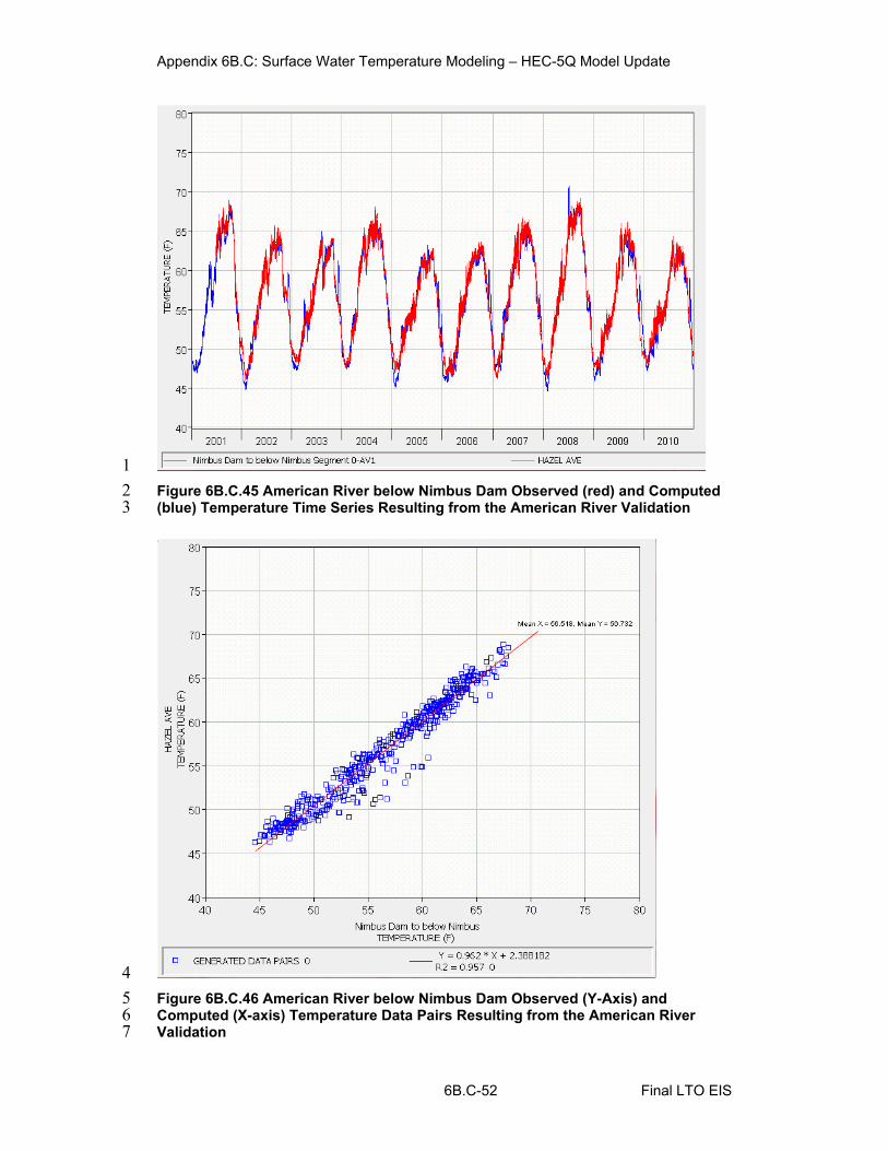
Appendix 6B.C: Surface Water Temperature Modeling – HEC-5Q Model Update
1 2 3
Figure 6B.C.45 American River below Nimbus Dam Observed (red) and Computed (blue) Temperature Time Series Resulting from the American River Validation
4 5 6 7
Figure 6B.C.46 American River below Nimbus Dam Observed (Y-Axis) and Computed (X-axis) Temperature Data Pairs Resulting from the American River Validation
6B.C-52 Final LTO EIS

Appendix 6B.C: Surface Water Temperature Modeling – HEC-5Q Model Update
Table 6B.C.19 American River below Nimbus Dam Computed and Observed 1 2 Statistical Comparison
Period Values Computed
(oF) Observed
(oF) Bias (oF)
RMS Differences
(oF)
Mean Differences
(oF)
Jan 1108 47.54 48.53 -1.00 1.40 1.14
Feb 1016 47.71 48.21 -0.49 0.83 0.68
Mar 1116 51.03 50.71 0.32 1.29 1.05
Apr 1064 53.07 53.57 -0.50 0.96 0.78
May 1093 55.83 56.12 -0.29 0.90 0.69
Jun 1075 58.56 58.67 -0.11 0.84 0.66
Jul 1199 61.91 61.88 0.04 0.93 0.72
Aug 1192 63.08 63.08 0.00 0.89 0.68
Sep 1164 63.26 63.68 -0.42 0.99 0.82
Oct 1240 62.82 63.26 -0.44 0.66 0.56
Nov 1200 57.69 58.27 -0.58 1.05 0.88
Dec 1236 53.28 52.39 0.89 2.00 1.56
Jan-Mar 3240 48.79 49.18 -0.39 1.20 0.97
Apr-Jun 3232 55.83 56.13 -0.30 0.90 0.71
Jul-Sep 3555 62.75 62.87 -0.12 0.94 0.74
Oct-Dec 3676 57.94 57.97 -0.04 1.36 1.00
Average Year
13703 56.53 56.73 -0.20 1.12 0.86
Final LTO EIS 6B.C-53

Appendix 6B.C: Surface Water Temperature Modeling – HEC-5Q Model Update
1 2 3
Figure 6B.C.47 American River at William Pond Park Observed (red) and Computed (blue) Temperature Time Series Resulting from the American River Validation
4 5 6 7
Figure 6B.C.48 American River at William Pond Park Observed (Y-Axis) and Computed (X-axis) Temperature Data Pairs Resulting from the American River Validation
6B.C-54 Final LTO EIS

Appendix 6B.C: Surface Water Temperature Modeling – HEC-5Q Model Update
Table 6B.C.20 American River at William Pond Park Computed and Observed 1 2 Statistical Comparison
Period Values Computed
(oF) Observed
(oF) Bias (oF)
RMS Differences
(oF)
Mean Differences
(oF)
Jan 1198 47.78 48.68 -0.91 1.63 1.29
Feb 1121 48.51 48.75 -0.23 1.05 0.85
Mar 1219 52.35 51.80 0.54 1.39 1.12
Apr 1157 54.59 54.83 -0.24 1.16 0.92
May 1131 58.36 58.25 0.12 1.13 0.89
Jun 1196 60.62 60.27 0.34 1.07 0.84
Jul 1236 63.93 63.38 0.55 1.14 0.88
Aug 1232 65.15 64.94 0.22 1.09 0.86
Sep 1200 64.79 65.18 -0.39 1.17 0.93
Oct 1240 63.24 63.76 -0.52 0.98 0.78
Nov 1200 57.70 58.26 -0.56 1.13 0.90
Dec 1113 53.24 52.24 0.99 1.84 1.43
Jan-Mar 3538 49.58 49.78 -0.19 1.38 1.09
Apr-Jun 3484 57.88 57.81 0.08 1.12 0.88
Jul-Sep 3668 64.63 64.49 0.13 1.13 0.89
Oct-Dec 3553 58.24 58.30 -0.06 1.35 1.02
Average Year
14243 57.65 57.66 -0.01 1.25 0.97
Final LTO EIS 6B.C-55
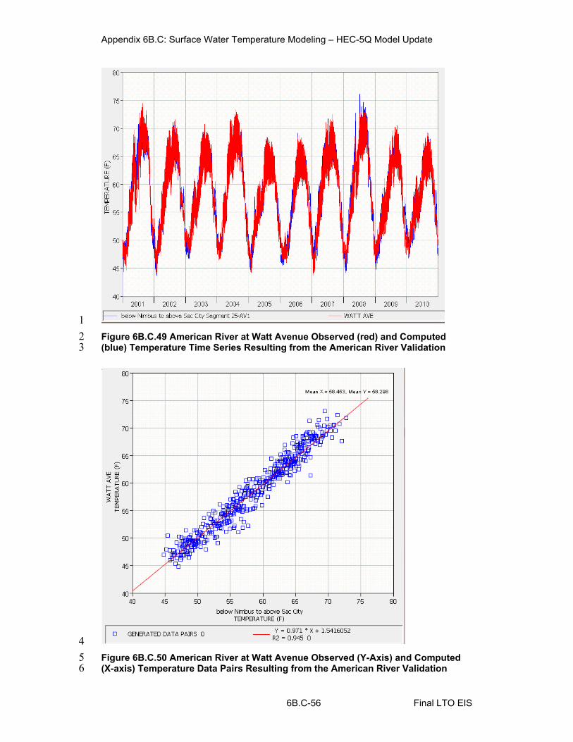
Appendix 6B.C: Surface Water Temperature Modeling – HEC-5Q Model Update
1 2 3
Figure 6B.C.49 American River at Watt Avenue Observed (red) and Computed (blue) Temperature Time Series Resulting from the American River Validation
4 5 6
Figure 6B.C.50 American River at Watt Avenue Observed (Y-Axis) and Computed (X-axis) Temperature Data Pairs Resulting from the American River Validation
6B.C-56 Final LTO EIS

Appendix 6B.C: Surface Water Temperature Modeling – HEC-5Q Model Update
Table 6B.C.21 American River at Watt Avenue Computed and Observed Statistical 1 2 Comparison
Period Values Computed
(oF) Observed
(oF) Bias (oF)
RMS Differences
(oF)
Mean Differences
(oF)
Jan 1223 47.91 48.48 -0.57 1.45 1.09
Feb 1128 49.14 49.11 0.02 1.02 0.83
Mar 1224 53.40 52.77 0.63 1.44 1.17
Apr 1153 55.98 55.99 0.00 1.26 1.02
May 1151 59.88 59.52 0.36 1.37 1.08
Jun 1200 62.20 61.43 0.77 1.89 1.35
Jul 1240 65.51 64.67 0.84 1.75 1.25
Aug 1236 66.64 66.42 0.22 1.40 1.16
Sep 1196 65.96 66.32 -0.36 1.38 1.14
Oct 1240 63.58 64.03 -0.46 1.01 0.84
Nov 1188 57.72 58.06 -0.35 1.05 0.83
Dec 1232 52.76 51.95 0.81 1.91 1.57
Jan-Mar 3575 50.18 50.15 0.02 1.33 1.04
Apr-Jun 3504 59.39 59.01 0.38 1.54 1.15
Jul-Sep 3672 66.04 65.80 0.24 1.52 1.18
Oct-Dec 3660 58.04 58.03 0.01 1.39 1.08
Average Year
14411 58.46 58.29 0.16 1.45 1.11
6B.C.10 Trinity River Outlet Diagrams 3
4 5 6 7 8 9
10
Diagrams that were used to simulate the Trinity Dam selective withdrawal procedure and the associated updates to the Trinity Dam outlets in the Trinity-Sacramento HEC-5Q model are presented in this section. Figure 6B.C.51 shows a schematic of the Trinity Dam outlets. Figure 6B.C.52 shows outlet capacity curves for the different Trinity Dam outlets. Figure 6B.C.53 shows the operational and flow vs. head (0 feet head at 1,900 feet lake elevation) characteristics of the Trinity Dam retrofitted turbine.
Final LTO EIS 6B.C-57

Appendix 6B.C: Surface Water Temperature Modeling – HEC-5Q Model Update
1
2
Figure 6B.C.51 Schematic of Trinity Dam Outlets (Wahl and Cohen 1999)
3
4 5
Figure 6B.C.52 Outlet Capacity Curves for Trinity Dam Outlets (Wahl and Cohen 1999)
6B.C-58 Final LTO EIS

Appendix 6B.C: Surface Water Temperature Modeling – HEC-5Q Model Update
1 2 3
Figure 6B.C.53 Operational and Flow Compared to Total Head (with 0 feet head at 1,900 feet lake elevation) Characteristics of the Trinity Dam Retrofitted Turbine
Final LTO EIS 6B.C-59

Appendix 6B.C: Surface Water Temperature Modeling – HEC-5Q Model Update
6B.C.11 Shasta Release Temperature Target 1 2
3 4 5 6 7
8 9
10 11 12 13 14 15
16 17
18 19 20 21
22 23
24
25 26
Schedules Spreadsheet Development
An approach to setting Shasta Dam release temperature target schedules in accordance with the 2009 NMFS BO, current management of the temperature target locations, and the spreadsheet tool SacR_Temp_Sel_Tool_rev05_FULL_FINAL_3-3-15.xlsm are presented in this section.
6B.C.11.1 Background The SWRCB Water Rights Order 90-05 and NMFS BO include water temperature criteria in Sacramento River downstream of Shasta Dam. The NMFS BO Reasonable and Prudent Alternative (RPA) I.2.1 sets forth temperature compliance percentages for the summer season at specified locations on the Sacramento River (Table 6B.C.22) for not exceeding 56⁰F at the specified location. These compliance percentages do not apply during extended drought periods.
Table 6B.C.22 Compliance Percentage for Not Exceeding 56⁰F at Select Locations on the Sacramento River in the NMFS BO
Location Compliance Percentage in NMFS BO (based
on 10-year moving average)
Clear Creek 95 percent of Time
Balls Ferry 85 percent of Time
Jelly’s Ferry 40 percent of Time
Bend Bridge 15 percent of Time
Shasta Lake releases are operated to not exceed 56⁰F at the compliance locations, to the extent possible. The Sacramento River Temperature Task Group (SRTTG) meets once a month from April to October to discuss temperature compliance actions, as described in Appendix 3A.
Historically, initial compliance locations have been correlated to End-of-April storage, as summarized in Table 6B.C.23.
Table 6B.C.23 Compliance Location Based Upon End-of-April Storage Compliance Location End-of-April Storage (TAF)
Clear Creek <3600
Balls Ferry 3600 – 4000
Jelly’s Ferry 4000 – 4400
Bend Bridge >4400
Figure 6B.C.54 shows the temperature compliance from 1996 to 2014 based on monthly Sacramento River Temperature Reports (Reclamation 2015). Shasta
6B.C-60 Final LTO EIS

Appendix 6B.C: Surface Water Temperature Modeling – HEC-5Q Model Update
Dam releases were operated under SWRCB Water Rights Order 90-05 during this 1 2
3 4
5 6 7 8 9
10 11
12 13 14 15 16 17 18 19 20
21 22 23 24
entire time period. Operations under the NMFS BO were initiated in 2009.
Figure 6B.C.54 Temperature Compliance Locations from 1996 through 2014
0
10
20
30
40
50
60
1-Oct 31-Oct 30-Nov 30-Dec 29-Jan 28-Feb 30-Mar 29-Apr 29-May 28-Jun 28-Jul 27-Aug 26-Sep
Dist
ance
from
Sha
sta
(Riv
er-m
ile)
WY 2014 - Critical WY 2013 - Dry WY 2012 - Below NormalWY 2011 - Wet WY 2010 - Below Normal WY 2009 - DryWY 2008 - Critical WY 2007 - Dry WY 2006 - WetWY 2005 - Above Normal WY 2004 - Below Normal WY 2003 - Above NormalWY 2002 - Dry WY 2001 - Dry WY 2000 - Above NormalWY 1999 - Wet WY 1998 - Wet WY 1997 - Wet
Bend Bridge
Jelly’s Ferry
Balls Ferry
Airport RoadClear Creek
As shown in Figure 6B.C.54, the compliance location often changed multiple times in a year as Shasta storage, meteorology, tributary, and fisheries conditions changed through the year. No specific procedure could be identified for when locations were changed. In some years, such as 2007, the location would start further downstream (Bend Bridge), then move upstream (Balls Ferry), then move downstream (Jelly’s Ferry), and then back upstream (Balls Ferry). In other years (e.g., 2004), the location would progressively move upstream.
Two general trends were identified. First, the compliance locations tended to be at Balls Ferry, Airport Road, and/or Clear Creek in dryer years (when Shasta Lake storage was low with less cold-water), and at Jelly’s Ferry and Bend Bridge in wetter years. Second, the compliance location tended to move closer to Shasta Dam later in the year (as the cold-water pool became more depleted and meteorological conditions became warmer). These two trends, combined with the general operations used by Reclamation to set the initial annual compliance location, were used to help develop the temperature scheduling logic described below.
6B.C.11.2 Temperature Target Spreadsheet Development This section describes the development of the Sacramento River Temperature Targeting Spreadsheet SacR_Temp_Sel_Tool_rev05_FULL_FINAL_3-3-15.xlsm.
Final LTO EIS 6B.C-61

Appendix 6B.C: Surface Water Temperature Modeling – HEC-5Q Model Update
Shasta storage data from the CalSim II EIS No Action Alternative Q5 run dated 1 2 3 4 5 6 7 8 9
10 11
12 13 14
15 16 17
18 19 20 21 22 23 24 25 26
27 28 29 30 31 32
33 34 35 36 37 38 39 40 41 42 43 44
January 27, 2015 was loaded into the spreadsheet. This storage data set the compliance location for each year of the CalSim II simulation period and the data remain unchanged throughout the temperature schedule development. April storage was chosen as the parameter from which to choose the compliance location because it was specified as the indicator of cold-water pool storage in the NMFS BO. April storage was divided into five tiers, each tier representing a different compliance location based on Reclamation’s rule-of-thumb approach for Shasta End-of-April storage shown in Table 6B.C.23. (Note that the storage tier for compliance with Jelly’s Ferry is at 4,425 TAF in this procedure instead of 4,400 TAF.)
The four compliance locations (see Table 6B.C.22) were given an annual temperature schedule of monthly Shasta release temperature targets. These targets were developed using the following logic.
• Step 1: For each month individually, the difference between the modeledtemperature at the compliance location and the modeled temperature belowShasta Dam was calculated for each year.
• Step 2: The difference value calculated in Step 1 that represented a specifiedexceedance for each month was then calculated for all compliance locations.This helped characterize the warming that occurred between Shasta releasetemperatures and each compliance location. For example, September at BendBridge was given a 5 percent exceedance. This exceedance says that only5 percent of years had a September temperature difference higher than thisdifference value (e.g. 11.2⁰F). In other words, warming that occurredbetween Shasta and Bend Bridge in September for the previous model run was11.2⁰F or lower for 95 percent of years.
• Step 3: The value calculated in Step 2 was then subtracted from 56⁰F and thisbecame the Shasta release temperature target for that compliance location inthat month. This step assumes that the Shasta release temperature target willmeet 56⁰F or lower at the compliance location for the exceedance percentagenumber of years. For example, a Shasta release temperature target of 44.8⁰Fin September will meet 56⁰F or lower at Bend Bridge for 95 percent of years.
The Sacramento River HEC-5Q model was run, using the January 13, 2015 version delivered to Reclamation and the CalSim II data described in previously, and the temperature output was loaded into the spreadsheet. The compliance performance was checked by calculating the percentage of years, over the 81-year simulation period, each compliance location exceeded 56⁰F for each month and the difference between that percentage and the compliance percentage listed in Table 6B.C.22. Then, using an initial set of exceedance percentages (described in Step 2) and the latest Sacramento River HEC-5Q model code (March 3, 2015) to set the new temperature schedules, the Sacramento River HEC-5Q model was re-run and the temperature output reloaded in the spreadsheet. An iterative process was then performed where the exceedance percentages were adjusted, the Sacramento River HEC-5Q model was re-run and the temperature output was
6B.C-62 Final LTO EIS

Appendix 6B.C: Surface Water Temperature Modeling – HEC-5Q Model Update
reloaded, and the compliance performance was checked until the compliance 1 2 3
4 5
performance was deemed satisfactory. The final exceedance percentages (June to December) are listed in Table 6B.C.24.
Table 6B.C.24 Exceedance Percentages for June through December at the Four Temperature Compliance Locations
June July August September October November December
Clear Creek 75.00 50.00 15.00 5.00 25.00 40.00 50.00
Balls Ferry 75.00 50.00 15.00 5.00 25.00 40.00 50.00
Jelly’s Ferry 75.00 50.00 15.00 5.00 25.00 40.00 50.00
Bend Bridge 75.00 50.00 15.00 5.00 25.00 40.00 50.00
January through May were not given exceedance percentages as temperature 6789
1011121314151617
1819
202122
management during those months is generally not an issue. Instead, January, February, and March were given a constant temperature target of 60.8⁰F, which is the average temperature above the thermocline in Lake Shasta. Shasta Lake generally does not stratify during those months so the temperature at the top of the thermocline is assumed to be consistent through the entire depth of Shasta Lake (Rettig and Bortleson 1983). April and May were given a constant temperature of 53.6⁰F, which is the average temperature below the thermocline in Shasta Lake. Stratification starts to occur in April and May and it is assumed that there is enough storage in Shasta Lake to conserve the cold-water pool. The final Shasta release temperature targets used in the spreadsheet for each compliance location are shown in Table 6B.C.25.
Table 6B.C.25 Final Shasta Lake Release Temperature Targets Used in the Temperature Targeting Spreadsheet
Location
Shasta Storage (TAF) Jan Feb Mar Apr May Jun Jul Aug Sep Oct Nov Dec
None <2000 60.8 60.8 60.8 53.6 53.6 52.6 52.6 51.8 50.8 54.6 56.0 56.2
Clear Creek
<3600 60.8 60.8 60.8 53.6 53.6 52.6 52.6 51.8 50.8 54.6 56.0 56.2
Balls Ferry
<4000 60.8 60.8 60.8 53.6 53.6 51.2 51.5 50.4 49.3 54.1 56.3 56.9
Jelly’s Ferry
<4425 60.8 60.8 60.8 53.6 53.6 49.6 50.1 48.7 47.7 53.6 56.7 57.6
Bend Bridge
<9999 60.8 60.8 60.8 53.6 53.6 48.5 49.0 47.4 46.6 53.4 56.9 58.1
This modeling approach does not dynamically change the compliance location that in reality changes throughout the year based on the SRTTG recommendations. While the temperature release targets would not change using
Final LTO EIS 6B.C-63

Appendix 6B.C: Surface Water Temperature Modeling – HEC-5Q Model Update
for the year with this modeling logic, the logic recognizes that those temperature 1 2 3 4 5 6 7
8 9
10 11 12 13 14 15 16 17 18 19 20 21 22 23 24 25
release targets will not be possible to meet in each year due to changes in Shasta Lake storage and meteorological conditions. If modeled Shasta Lake releases are lower than the temperature target, then it could be considered that the compliance location was moved downstream. In addition, if Shasta Lake releases are higher than the temperature target, then it could be considered that the compliance location was moved upstream.
As an example, the End-of-April Storage from the CalSim II run in Year 1940 is 4,140 TAF. The compliance location is therefore set to be Jelly’s Ferry and the temperature schedule in Table 6B.C.25 is for Jelly’s Ferry. Using those temperature targets, the HEC-5Q model run produces Shasta Lake outflow temperatures that do not meet those temperature targets and thus result in temperatures that do not meet 56⁰F at Jelly’s Ferry, due to Shasta Lake storage and downstream meteorological conditions. For instance, in July the Shasta Lake outflow was 48.6⁰F, even though the release target was 50.1⁰F. This is because Shasta Lake storage was still relatively high to preserve more cold water in the reservoir pool and meteorological conditions were cooler than were typical for July. Thus the release temperature was cooler than the temperature target and as a result, 56⁰F was met at Bend Bridge. In September, Shasta Lake outflow was 53.7⁰F, even though the temperature target was 47.7⁰F. This is because meteorological conditions were warmer than were typical for September. Thus the release temperature was warmer than the temperature target and as result, 56⁰F could only be met at Clear Creek. A full illustration of modeled Year 1940 and the compliance location changes based on Shasta release temperatures are presented on Figure 6B.C.55.
26 27 28
Figure 6B.C.55 Changes in Compliance Location Based on Shasta Lake Release Temperatures for Year 1940
Year 1940 –Above Normal
End-of-April Shasta Storage
= 4140 TAF
Compliance Location = Jellys Ferry
Temperature TargetsJun = 49.6⁰ FJul = 50.1⁰ F
Aug = 48.7⁰ FSep = 47.7⁰ FOct = 53.6⁰ FNov = 56.7⁰ FDec = 57.6⁰ F
Shasta Release TemperaturesJun = 47.0⁰ FJul = 48.6⁰ F
Aug = 50.9⁰ FSep = 53.7⁰ FOct = 55.8⁰ FNov = 55.7⁰ FDec = 52.2⁰ F
Compliance LocationJun = Bend BridgeJul = Bend BridgeAug = Balls FerrySep = Clear Creek
Oct = NoneNov = Bend BridgeDec = Bend Bridge
6B.C-64 Final LTO EIS

Appendix 6B.C: Surface Water Temperature Modeling – HEC-5Q Model Update
While during all months the temperature target was set based on a compliance 1 2 3 4
5 6 7
location of Jelly’s Ferry, the actual compliance location changed. Thus the model passively mimics the SRTTG changing the compliance location based on Shasta Lake storage conditions and downstream meteorological conditions.
The chosen compliance location based on End-of-April storage and the actual compliance location achieved over the 81-year simulation period are shown on Figure 6B.C.56.
Final LTO EIS 6B.C-65

Appendix 6B.C: Surface Water Temperature Modeling – HEC-5Q Model Update
1 2 3
Figure 6B.C.56 Simulated Compliance Location Target and Achievement for Each Year over the 81-Year CalSim II Period
Year WYT Target May June July August September October November December1922 AN Jellys Ferry Clear Creek None None None None None Bend Bridge Bend Bridge1923 BN Clear Creek Bend Bridge Jellys Ferry None None None None Bend Bridge Bend Bridge1924 C Clear Creek Clear Creek None Balls Ferry None None None Bend Bridge Bend Bridge1925 D Balls Ferry Bend Bridge Bend Bridge Bend Bridge Jellys Ferry Balls Ferry Jellys Ferry Bend Bridge Bend Bridge1926 D Balls Ferry Bend Bridge Bend Bridge Jellys Ferry None None None Bend Bridge Bend Bridge1927 W Bend Bridge Bend Bridge Bend Bridge Bend Bridge Bend Bridge Jellys Ferry Bend Bridge Bend Bridge Bend Bridge1928 AN Bend Bridge Jellys Ferry Bend Bridge Bend Bridge Jellys Ferry Clear Creek None Bend Bridge Bend Bridge1929 C Clear Creek Bend Bridge Jellys Ferry Balls Ferry None None None Bend Bridge Bend Bridge1930 D Clear Creek Jellys Ferry Jellys Ferry Balls Ferry None None None Bend Bridge Bend Bridge1931 C None Jellys Ferry Clear Creek None None None None Bend Bridge Bend Bridge1932 D None Balls Ferry Clear Creek None None None None Bend Bridge Bend Bridge1933 C None Jellys Ferry Clear Creek None None None None Bend Bridge Bend Bridge1934 C None Jellys Ferry Clear Creek None None None None Bend Bridge Bend Bridge1935 BN Clear Creek Balls Ferry Jellys Ferry Balls Ferry None None None Bend Bridge Bend Bridge1936 BN Balls Ferry Bend Bridge Bend Bridge Bend Bridge Balls Ferry Clear Creek Clear Creek Bend Bridge Bend Bridge1937 BN Balls Ferry Balls Ferry Jellys Ferry Balls Ferry Balls Ferry None Clear Creek Bend Bridge Bend Bridge1938 W Jellys Ferry Bend Bridge Balls Ferry Balls Ferry Jellys Ferry Jellys Ferry Balls Ferry Bend Bridge Bend Bridge1939 D Clear Creek Bend Bridge Bend Bridge Jellys Ferry None None None Bend Bridge Bend Bridge1940 AN Jellys Ferry Jellys Ferry Bend Bridge Bend Bridge Balls Ferry Clear Creek None Bend Bridge Bend Bridge1941 W Bend Bridge Bend Bridge Bend Bridge Jellys Ferry Jellys Ferry Bend Bridge Bend Bridge Bend Bridge Bend Bridge1942 W Jellys Ferry Bend Bridge Jellys Ferry Bend Bridge Bend Bridge Bend Bridge Bend Bridge Bend Bridge Bend Bridge1943 W Bend Bridge Bend Bridge Bend Bridge Bend Bridge Bend Bridge Bend Bridge Balls Ferry Bend Bridge Bend Bridge1944 D Clear Creek Jellys Ferry Bend Bridge Jellys Ferry Clear Creek None None Bend Bridge Bend Bridge1945 BN Balls Ferry Bend Bridge Bend Bridge Bend Bridge Jellys Ferry Balls Ferry Bend Bridge Bend Bridge Bend Bridge1946 BN Jellys Ferry Bend Bridge Bend Bridge Bend Bridge Bend Bridge Jellys Ferry Clear Creek Bend Bridge Bend Bridge1947 D Clear Creek Bend Bridge Bend Bridge Jellys Ferry None None None Bend Bridge Bend Bridge1948 BN Jellys Ferry Jellys Ferry Balls Ferry Bend Bridge Jellys Ferry Balls Ferry Bend Bridge Bend Bridge Bend Bridge1949 D Jellys Ferry Bend Bridge Bend Bridge Bend Bridge Jellys Ferry Clear Creek Bend Bridge Bend Bridge Bend Bridge1950 BN Balls Ferry Jellys Ferry Bend Bridge Jellys Ferry Balls Ferry Clear Creek Bend Bridge Bend Bridge Bend Bridge1951 AN Jellys Ferry Jellys Ferry Bend Bridge Bend Bridge Bend Bridge Jellys Ferry Bend Bridge Bend Bridge Bend Bridge1952 W Jellys Ferry Bend Bridge Jellys Ferry Jellys Ferry Jellys Ferry Bend Bridge Bend Bridge Bend Bridge Bend Bridge1953 W Bend Bridge Bend Bridge Jellys Ferry Bend Bridge Jellys Ferry Bend Bridge Bend Bridge Bend Bridge Bend Bridge1954 AN Bend Bridge Bend Bridge Bend Bridge Bend Bridge Jellys Ferry Jellys Ferry Bend Bridge Bend Bridge Bend Bridge1955 D Balls Ferry Balls Ferry Bend Bridge Bend Bridge Clear Creek None Jellys Ferry Bend Bridge Bend Bridge1956 W Bend Bridge Bend Bridge Bend Bridge Bend Bridge Bend Bridge Bend Bridge Bend Bridge Bend Bridge Bend Bridge1957 AN Bend Bridge Bend Bridge Jellys Ferry Bend Bridge Jellys Ferry Balls Ferry Jellys Ferry Bend Bridge Bend Bridge1958 W Jellys Ferry Balls Ferry Balls Ferry Jellys Ferry Jellys Ferry Bend Bridge Clear Creek Bend Bridge Bend Bridge1959 BN Jellys Ferry Bend Bridge Bend Bridge Jellys Ferry Clear Creek None None Bend Bridge Bend Bridge1960 D Jellys Ferry Balls Ferry Bend Bridge Bend Bridge Balls Ferry None None Bend Bridge Bend Bridge1961 D Jellys Ferry Bend Bridge Bend Bridge Bend Bridge Jellys Ferry Clear Creek Balls Ferry Bend Bridge Bend Bridge1962 BN Bend Bridge Bend Bridge Bend Bridge Bend Bridge Jellys Ferry Clear Creek Jellys Ferry Bend Bridge Bend Bridge1963 W Jellys Ferry Balls Ferry Jellys Ferry Bend Bridge Balls Ferry Jellys Ferry Clear Creek Bend Bridge Bend Bridge1964 D Balls Ferry Bend Bridge Bend Bridge Bend Bridge Balls Ferry None Clear Creek Bend Bridge Bend Bridge1965 W Bend Bridge Bend Bridge Bend Bridge Bend Bridge Jellys Ferry Bend Bridge Bend Bridge Bend Bridge Bend Bridge1966 BN Jellys Ferry Bend Bridge Bend Bridge Bend Bridge Jellys Ferry Balls Ferry Clear Creek Bend Bridge Bend Bridge1967 W Bend Bridge Bend Bridge Balls Ferry Jellys Ferry Balls Ferry Bend Bridge Bend Bridge Bend Bridge Bend Bridge1968 BN Jellys Ferry Bend Bridge Bend Bridge Bend Bridge Balls Ferry Clear Creek Balls Ferry Bend Bridge Bend Bridge1969 W Bend Bridge Bend Bridge Bend Bridge Bend Bridge Jellys Ferry Balls Ferry Bend Bridge Bend Bridge Bend Bridge1970 W Jellys Ferry Bend Bridge Bend Bridge Bend Bridge Jellys Ferry Balls Ferry Balls Ferry Bend Bridge Bend Bridge1971 W Jellys Ferry Bend Bridge Jellys Ferry Bend Bridge Balls Ferry Jellys Ferry Bend Bridge Bend Bridge Bend Bridge1972 BN Bend Bridge Bend Bridge Bend Bridge Bend Bridge Balls Ferry None Bend Bridge Bend Bridge Bend Bridge1973 AN Jellys Ferry Balls Ferry Bend Bridge Bend Bridge Jellys Ferry Jellys Ferry Bend Bridge Bend Bridge Bend Bridge1974 W Jellys Ferry Jellys Ferry Jellys Ferry Jellys Ferry Balls Ferry Bend Bridge Bend Bridge Bend Bridge Bend Bridge1975 W Jellys Ferry Bend Bridge Jellys Ferry Jellys Ferry Balls Ferry Bend Bridge Jellys Ferry Bend Bridge Bend Bridge1976 C Balls Ferry Bend Bridge Jellys Ferry Balls Ferry None None Balls Ferry Bend Bridge Bend Bridge1977 C None Jellys Ferry Clear Creek None None None None Bend Bridge Bend Bridge1978 AN Bend Bridge Bend Bridge Bend Bridge Bend Bridge Jellys Ferry Balls Ferry Balls Ferry Bend Bridge Bend Bridge1979 BN Balls Ferry Balls Ferry Bend Bridge Jellys Ferry Clear Creek None Clear Creek Bend Bridge Bend Bridge1980 AN Jellys Ferry Bend Bridge Bend Bridge Bend Bridge Jellys Ferry Balls Ferry Bend Bridge Bend Bridge Bend Bridge1981 D Jellys Ferry Bend Bridge Bend Bridge Jellys Ferry Clear Creek None None Bend Bridge Bend Bridge1982 W Jellys Ferry Balls Ferry Jellys Ferry Jellys Ferry Balls Ferry Balls Ferry Bend Bridge Bend Bridge Bend Bridge1983 W Jellys Ferry Jellys Ferry Balls Ferry Balls Ferry Balls Ferry Balls Ferry Balls Ferry Bend Bridge Bend Bridge1984 W Bend Bridge Bend Bridge Bend Bridge Bend Bridge Balls Ferry Jellys Ferry Clear Creek Bend Bridge Bend Bridge1985 D Balls Ferry Bend Bridge Bend Bridge Jellys Ferry Clear Creek None None Bend Bridge Bend Bridge1986 W Balls Ferry Bend Bridge Bend Bridge Bend Bridge Balls Ferry Clear Creek Clear Creek Bend Bridge Bend Bridge1987 D Clear Creek Bend Bridge Bend Bridge Jellys Ferry None None None Bend Bridge Bend Bridge1988 C Clear Creek Bend Bridge Bend Bridge Balls Ferry None None None Bend Bridge Bend Bridge1989 D Balls Ferry Bend Bridge Jellys Ferry Jellys Ferry None None None Bend Bridge Bend Bridge1990 C Clear Creek Balls Ferry Balls Ferry Clear Creek None None None Bend Bridge Bend Bridge1991 C Clear Creek Jellys Ferry Balls Ferry None None None None None Bend Bridge1992 C Clear Creek Jellys Ferry Clear Creek None None None None None Bend Bridge1993 AN Jellys Ferry Jellys Ferry Balls Ferry Bend Bridge Balls Ferry Balls Ferry Balls Ferry Bend Bridge Bend Bridge1994 C Clear Creek Balls Ferry Bend Bridge Clear Creek None None None Bend Bridge Bend Bridge1995 W Jellys Ferry Bend Bridge Balls Ferry Balls Ferry Balls Ferry Balls Ferry Jellys Ferry Bend Bridge Bend Bridge1996 W Jellys Ferry Bend Bridge Balls Ferry Balls Ferry Clear Creek Clear Creek None Bend Bridge Bend Bridge1997 W Balls Ferry Bend Bridge Bend Bridge Bend Bridge Clear Creek None Clear Creek Bend Bridge Bend Bridge1998 W Jellys Ferry Bend Bridge Balls Ferry Balls Ferry Balls Ferry None Clear Creek Bend Bridge Bend Bridge1999 W Bend Bridge Bend Bridge Jellys Ferry Bend Bridge Balls Ferry Jellys Ferry Balls Ferry Bend Bridge Bend Bridge2000 AN Bend Bridge Balls Ferry Bend Bridge Bend Bridge Balls Ferry Clear Creek None Bend Bridge Bend Bridge2001 D Balls Ferry Bend Bridge Bend Bridge Balls Ferry None None None Bend Bridge Bend Bridge2002 D Jellys Ferry Bend Bridge Bend Bridge Bend Bridge Balls Ferry Clear Creek Bend Bridge Bend Bridge Bend Bridge
6B.C-66 Final LTO EIS
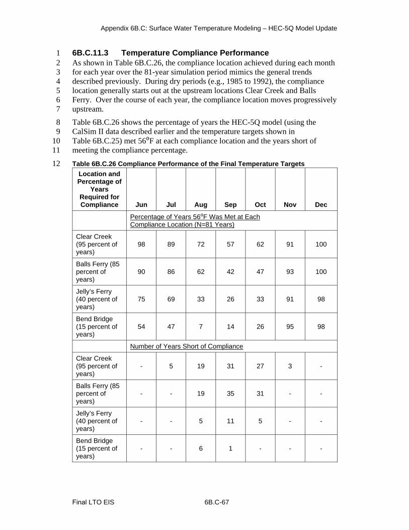
Appendix 6B.C: Surface Water Temperature Modeling – HEC-5Q Model Update
Final LTO EIS 6B.C-67
6B.C.11.3 Temperature Compliance Performance 1 2 3 4 5 6 7
8 9
10 11
12
As shown in Table 6B.C.26, the compliance location achieved during each month for each year over the 81-year simulation period mimics the general trends described previously. During dry periods (e.g., 1985 to 1992), the compliance location generally starts out at the upstream locations Clear Creek and Balls Ferry. Over the course of each year, the compliance location moves progressively upstream.
Table 6B.C.26 shows the percentage of years the HEC-5Q model (using the CalSim II data described earlier and the temperature targets shown in Table 6B.C.25) met 56⁰F at each compliance location and the years short of meeting the compliance percentage.
Table 6B.C.26 Compliance Performance of the Final Temperature Targets Location and Percentage of
Years Required for Compliance Jun Jul Aug Sep Oct Nov Dec
Percentage of Years 56⁰F Was Met at Each Compliance Location (N=81 Years)
Clear Creek (95 percent of years)
98 89 72 57 62 91 100
Balls Ferry (85 percent of years)
90 86 62 42 47 93 100
Jelly’s Ferry (40 percent of years)
75 69 33 26 33 91 98
Bend Bridge (15 percent of years)
54 47 7 14 26 95 98
Number of Years Short of Compliance
Clear Creek (95 percent of years)
- 5 19 31 27 3 -
Balls Ferry (85 percent of years)
- - 19 35 31 - -
Jelly’s Ferry (40 percent of years)
- - 5 11 5 - -
Bend Bridge (15 percent of years)
- - 6 1 - - -
Appendix 6B.C: Surface Water Temperature Modeling – HEC-5Q Model Update
6B.C.12 Folsom Release Temperature Target 1 2
3 4 5 6 7
8 9
10 11
12 13 14 15 16 17 18 19 20 21 22 23
24 25 26 27 28 29 30
31 32 33 34
35 36 37 38 39 40 41
Schedules Spreadsheet Development
An approach to setting Folsom Dam release temperature target schedules for temperature management on the Lower American River based on NMFS BO and is an accompanying document to the spreadsheet tool AmerR_Temp_Sel_Tool_rev15_FULL_FINAL_3-16-15.xlsm is presented in this section.
6B.C.12.1 Background The NMFS BO RPA II.2 sets forth a temperature requirement for the Lower American River at the Watt Avenue Bridge to not exceed 65⁰F from May 15 to October 31.
In order to meet the NMFS BO temperature requirement, Reclamation manages Folsom Dam release temperatures based on temperature schedules set forth in Appendix 2-D of the NMFS BO. These schedules set monthly temperatures at Watt Avenue for Folsom Dam to operate to from May to October (temperature management season) based on forecasted Folsom storage and inflow. The initial temperature schedule for each year is determined based on an operations plan developed by Reclamation and approved by the American River Operations Group (ARG). However, these schedules are based on forecasted conditions. As conditions actually happen throughout the temperature management season, due to changes in Folsom Lake storage and inflow, current meteorological conditions, and/or the state of fisheries in the river, the Watt Avenue temperature target schedule is adjusted based on recommendations from the ARG.
It was possible to model the initial annual temperature target schedule for Folsom Lake to operate to for the year because storage and forecasted inflow are known quantities in CalSim II. However, modeling the dynamic adjustment of the Watt Avenue temperature target based on current storage and meteorological conditions was not going to be possible. Thus logic was developed to create a temperature target selection procedure that set a specific schedule for each year that remained unchanged. This logic is described in the following section.
6B.C.12.2 Temperature Target Spreadsheet Development The development of the Sacramento River Temperature Targeting Spreadsheet AmerR_Temp_Sel_Tool_rev15_FULL_FINAL_3-16-15.xlsm is described in this section.
Folsom storage and inflow data from the CalSim II EIS No Action Alternative Q5 run dated January 27, 2015 was loaded into the spreadsheet. This CalSim II data remained unchanged throughout the temperature schedule development. May Folsom Storage plus June to September average inflow to Folsom (storage plus inflow) was calculated in the spreadsheet. This was a simplification of the forecasting approach that is used to set the actual temperature targets, as it only took into account June through September inflow.
6B.C-68 Final LTO EIS

Appendix 6B.C: Surface Water Temperature Modeling – HEC-5Q Model Update
Appendix 2-D of the NMFS BO lists 72 different temperature target schedules for 1 2 3 4 5 6 7 8 9
10 11 12 13 14 15 16
17 18 19
20 21
22 23
May through October. Each schedule changed the temperature target for one month only. It was deemed unnecessary to incorporate all 72 schedules due to the simplified forecasting approach described above that only focused on June to September inflow. This reduced the 72 schedules to schedules that focused primarily on temperature management during June through September. Ultimately the 72 schedules were reduced to 22 schedules as these schedules were deemed to adequately represent the variance in temperature targets during June through September.
Then, using an initial set of storage plus inflow tiers assigned to each temperature schedule number, the schedule number for each year of the CalSim II period of record was calculated. Then the average storage plus inflow for each tier was calculated. For example, there were 8 years over the simulation period that had a schedule number of 11 and the average storage plus inflow was 1,415 TAF. The average storage plus inflow calculated for each tier was plotted versus the schedule number, as shown in Figure 6B.C.57.
Figure 6B.C.57 Temperature Schedule Number and Average Folsom Lake Storage plus June-September Inflow for each Schedule Number
0
5
10
15
20
250 500 1000 1500 2000 2500
Tem
pera
ture
Sch
edul
e
Storage plus Inflow (TAF)
Average perSchedule Storageplus Inflow
Storage plus InflowTeirs Curve
The schedule shown in the plot was used to calculate the final storage plus inflow tiers used in the spreadsheet.
Using the regression equation shown in Figure 6B.C.57, the final storage plus inflow tiers to be used for the spreadsheet were calculated (see Table 6B.C.27).
Final LTO EIS 6B.C-69

Appendix 6B.C: Surface Water Temperature Modeling – HEC-5Q Model Update
Table 6B.C.27 Final Watt Avenue Temperature Target Schedules (Yellow 1 2 highlighted cells indicate a change from the previous schedule)
Schedule
Storage plus
June-Sept. Inflow Jan Feb Mar Apr May Jun Jul Aug Sep Oct Nov Dec
1 0 56 56 56 63 61 61 62 62 61 57 56 56
2 600 56 56 56 63 62 62 62 62 62 58 56 56
3 700 56 56 56 63 62 62 63 63 62 59 57 56
4 750 56 56 56 63 63 63 63 63 63 60 57 56
5 850 56 56 56 63 63 63 64 64 63 60 58 56
6 900 56 56 56 63 64 64 64 64 64 60 58 56
7 1000 56 56 56 63 64 64 65 65 64 60 58 56
8 1050 56 56 56 63 65 65 65 65 65 60 58 56
9 1150 56 56 56 63 65 65 66 66 65 65 59 56
10 1200 56 56 56 63 66 66 66 66 66 65 59 56
11 1300 56 56 56 63 66 66 67 67 66 65 59 56
12 1350 56 56 56 63 67 67 67 67 67 65 59 56
13 1450 56 56 56 63 67 67 68 68 67 65 59 56
14 1500 56 56 56 63 68 68 68 68 68 65 59 56
15 1600 56 56 56 63 68 68 69 69 68 68 59 56
16 1650 56 56 56 63 69 69 69 69 69 68 59 56
17 1750 56 56 56 63 69 69 70 70 69 69 60 56
18 1800 56 56 56 63 70 70 70 70 70 69 60 56
19 1900 56 56 56 63 70 70 71 71 70 70 61 56
20 1950 56 56 56 63 71 71 71 71 71 70 61 56
21 2050 56 56 56 63 71 71 72 72 71 71 62 56
22 2100 56 56 56 63 72 72 72 72 72 71 62 56
3 f4
5 6 7
8 9
t10 t11 t12
13 14 15 16 17
January, February, March and December were given temperature targets of 56⁰F or all temperature schedules as a default. During these months, temperature
management is generally not an issue. April was given a temperature target of 63⁰F to conserve cold water in the reservoir pool at the start of the temperature management season.
Establishing the temperature target schedule sets the temperature targets at Watt Avenue. However, Folsom Dam can only actually operate to release emperatures, with the goal that those release temperatures will ultimately meet he Watt Avenue temperature target after ambient warming occurs. To calculate he Folsom release temperatures, the following logic was developed.
• Step 1: The American River HEC-5Q Model was run using the January 13,2015 version delivered to Reclamation, the CalSim II data describedpreviously, and an initial Watt Avenue and Folsom Dam temperature targetschedules. The temperature output from that HEC-5Q model run was loadedinto the spreadsheet.
6B.C-70 Final LTO EIS

Appendix 6B.C: Surface Water Temperature Modeling – HEC-5Q Model Update
• 1 2 3
• 4 5 6 7 8 9
10 11
• 12 13 14
• 15 16 17 18
• 19 20
• 21 22
• 23 24 25 26
• 27 28 29 30 31 32 33
Step 2: For each month individually, the difference (shift) between the modeled temperature at Watt Avenue and the modeled temperature below Folsom Dam was calculated for each year.
Step 3: The annual shift calculated in Step 2 that represented a specified exceedance for each month was then calculated. This helped characterize the warming that occurred between Folsom release temperatures and Watt Avenue. For example, September was given a 50 percent exceedance. This exceedance says that 50 percent years had a September temperature shift higher than this shift value (e.g., 0.6⁰F). Therefore, warming that occurred between Folsom Dam and Watt Avenue in September for the previous model run was 0.6⁰F or lower for 95 percent of years.
Step 4: The exceedance shift value calculated in step iii was then divided by the average annual June to September shift value. This calculated a shift factor that was used in the final temperature shift calculations.
Step 5: The average June to September shift value for each schedule number was then calculated. For example, schedule number 11 was the schedule for eight years over the simulation period and the average June to September shift was 4.6⁰F.
Step 6: The average June to September shift value calculated in Step v was plotted versus its temperature schedule number, as shown in Figure 6B.C.58.
Step 7: Average June to September shifts for each schedule number were then calculated using the regression equation in Figure 6B.C.58.
Step 8: The shift values calculated in step vii were then multiplied by the shift factor calculated in step vii and was subtracted from the temperature target value in Table 6B.C.27. This created the Folsom Dam release temperature target schedules.
Step 9: An iterative process where the Folsom Dam temperature target schedules developed using the initial temperature target schedules described in step 1 were then used in the next HEC5Q model run and then reloaded into the spreadsheet. The process was repeated until the Folsom Dam release temperature target schedules were deemed acceptable based on modeled temperature results. The final Folsom Dam release temperature target schedules are shown in Table 6B.C.28.
Final LTO EIS 6B.C-71

Appendix 6B.C: Surface Water Temperature Modeling – HEC-5Q Model Update
1 2 3 4
5 6
7 8 9
Figure 6B.C.58 Average Temperature Shift between Modeled Folsom Lake Release Temperatures and Watt Avenue Temperatures for each Schedule Number after Multiple Iterations
0
1
2
3
4
5
6
7
8
9
100 5 10 15 20 25
Tem
pera
ture
Shi
ft (d
egre
ss F
)
Temperature Schedule
Average per ScheduleTemperature Shift
Shift Curve
The shift curve shown in the plot was used to calculate the final temperature shifts used in the spreadsheet.
Table 6B.C.28 Final Folsom Dam Lake Release Temperature Targets in the Spreadsheet (Yellow highlighted cells indicate a change from the previous schedule)
Storage Shift Factors plus
Jun-Sep 0.7 0.8 0.8 1.2 0.6 0.4 0.2 0
Schedule Inflow Jan Feb Mar Apr May Jun Jul Aug Sep Oct Nov Dec
1 0 52 52 52 59 66.8 66.0 66.0 63.0 67.5 68.0 60.5 56
2 600 52 52 52 59 66.8 66.0 66.0 63.0 67.5 68.0 60.5 56
3 700 52 52 52 59 65.9 65.2 66.2 63.3 66.7 68.1 60.6 56
4 750 52 52 52 59 66.3 65.6 65.6 62.9 67.0 67.3 59.7 56
5 850 52 52 52 59 65.6 65.0 66.0 63.5 66.3 67.5 59.8 56
6 900 52 52 52 59 65.8 65.2 65.2 62.8 66.4 66.6 58.8 56
7 1000 52 52 52 59 65.0 64.4 65.4 63.1 65.6 66.7 58.9 56
8 1050 52 52 52 59 65.2 64.6 64.6 62.4 65.7 65.8 57.9 56
9 1150 52 52 52 59 64.3 63.8 64.8 62.7 64.9 65.9 58.0 56
10 1200 52 52 52 59 64.5 64.0 64.0 62.0 65.0 63.0 58.0 56
11 1300 52 52 52 59 63.7 63.2 64.2 62.3 64.2 63.1 58.1 56
12 1350 52 52 52 59 63.7 63.2 63.2 61.3 64.2 63.1 58.1 56
6B.C-72 Final LTO EIS

Appendix 6B.C: Surface Water Temperature Modeling – HEC-5Q Model Update
Storage Shift Factors plus
Jun-Sep 0.7 0.8 0.8 1.2 0.6 0.4 0.2 0
Schedule Inflow Jan Feb Mar Apr May Jun Jul Aug Sep Oct Nov Dec
13 1450 52 52 52 59 62.9 62.4 63.4 61.6 63.3 63.2 58.1 56
14 1500 52 52 52 59 62.9 62.4 62.4 60.6 63.3 63.2 58.1 56
15 1600 52 52 52 59 61.9 61.4 62.4 60.6 62.3 63.2 58.1 56
16 1650 52 52 52 59 62.0 61.6 61.6 59.9 62.5 58.3 57.2 56
17 1750 52 52 52 59 61.0 60.6 61.6 59.9 61.5 58.3 57.2 56
18 1800 52 52 52 59 61.0 60.6 60.6 58.9 61.5 58.3 57.2 56
19 1900 52 52 52 59 60.0 59.6 60.6 58.9 60.5 58.3 57.2 56
20 1950 52 52 52 59 60.0 59.6 59.6 57.9 60.5 58.3 56.2 56
21 2050 52 52 52 59 59.0 58.6 59.6 57.9 59.5 57.3 56.2 56
22 2100 52 52 52 59 59.0 58.6 58.6 56.9 59.5 56.3 55.2 56
January through April were not given shift factors and instead were given a constant 4⁰F shift as a default for the same reason described for those months for the Watt Avenue temperature target schedules.
1 2 3
4 5 6
7 8
9 10 11
6B.C.12.3 Temperature Performance Figure 6B.C.59 shows box and whisker plots of modeled temperatures at Watt Avenue in the completed spreadsheet.
Figure 6B.C.59 Modeled Watt Avenue temperatures in Final Spreadsheet
62
66
6869
68
64
57
50
55
60
65
70
75
80
MAY JUN JUL AUG SEP OCT NOV
Mod
el W
att A
venu
e Te
mpe
ratu
re (⁰
F)
95%
75%
50%
25%
5%
The figure shows the expected pattern where temperatures are higher in the summer but the Watt Avenue target temperature for each month were met in majority of the years. The maximum temperature target (72⁰F) was not exceeded
Final LTO EIS 6B.C-73

Appendix 6B.C: Surface Water Temperature Modeling – HEC-5Q Model Update
i1 t2
3 s4
5
6 7 8
9 10
11 12 13
14 15 16
17 18 19
20 21 22 23
n approximately 75 percent of years for all months. The years where the emperatures exceeded the maximum 72⁰F target were during dry periods, when
meeting the Watt Avenue temperature targets are not possible to meet due to low torage in Folsom Lake.
6B.C.13 References
RMA (Resource Management Associates). 2003. Upper Sacramento River Water Quality Modeling with HEC-5Q: Model Calibration and Validation.
RMA (Resource Management Associates). 2013. Development of the American River HEC5Q Model.
Reclamation (Bureau of Reclamation Central Valley Operations Office). 2015 Sacramento River Temperature Report. Site accessed February 13, 2015. http://www.usbr.gov/mp/cvo/vungvari/sactemprpt.pdf
Rettig, S. and G. Bortleson. 1983. Limnological Study of Shasta Lake, Shasta County, California, with Emphasis on the Effects of the 1977 Drought. U.S. Geological Survey.
Smith, D., M. Deas, and N. Jayasundara. 2013. Extension of the Sacramento River Water Quality Model (SRWQM) to Include American and Feather River Representations.
Wahl, T.L. and E.A. Cohen. 1999. Determination of Controlled-Release Capacity from Trinity Dam. Proceedings from the 1999 International Water Resources Engineering Conference, American Society of Civil Engineers, August 8-11, 1999.
6B.C-74 Final LTO EIS

Appendix 6C: Methylmercury Model Documentation
5
10
15
20
25
30
35
1
2
3 4
6 7 8
9
11 12 13 14
16 17 18 19
21 22 23
24
26
27
28 29
31 32 33 34
36 37 38 39
Appendix 6C
Methylmercury M odel Documentation This appendix provides information about the methods, modeling tools, and assumptions used for the Coordinated Long-term Operation of the Central Valley Project (CVP) and State Water Project (SWP) Environmental Impact Statement (EIS) analysis. It also provides information pertaining to the development of the analytical tools and the use of input data as well as model result processing and interpretation methods used for the impacts analysis and descriptions.
This appendix is organized into three main sections that are briefly described below:
• Section 6C.1: Modeling Methodology. The methylmercury impacts analysis used CalSim II, the Delta Simulation Model II (DSM2), and the Central Valley Regional Water Quality Control Board (Central Valley RWQCB) Total Maximum Daily Load (TMDL) model (RWQCB Model) to assess and quantify effects of the alternatives on the long-term operations of the CVP and SWP and on the environment. This section provides information about the overall analytical framework and how some of the model input information obtained from other models was processed through the use of analytical tools.
• Section 6C.2: Modeling Simulations and Assumptions. This section provides a brief description of the assumptions for the RWQCB Model simulations of the No Action Alternative, Second Basis of Comparison, and Alternatives 1 through 5.
• Section 6C.3: Modeling Results. This section provides a description of the model simulation output formats used in the analysis and interpretation of modeling results for the alternatives impacts assessment.
6C.1 Modeling Methodology
This section summarizes the methylmercury modeling methodology used for the No Action Alternative, Second Basis of Comparison, and Alternatives 1 through 5. It describes the overall analytical framework and contains descriptions of the key analytical and numerical tools and approaches used in the quantitative evaluation of the alternatives. The alternatives include several major components that will have significant effects on SWP and CVP operations and minor effects on the water quality of the system.
6C.1.1 Overview of the Modeling Approach and Objectives Modeling of physical and biological methylmercury processes in the Delta is necessary to evaluate changes related to the implementation of alternatives that could affect the health of humans and wildlife consuming fish in the Delta. It has been recognized that fish tissue concentrations are the best indicator of mercury
Final Draft LTO EIS 6C-1

1 2 3 4 5 6
7 8 9
10 11 12 13 14 15 16 17 18
19 20 21 22
23 24
25 26 27 28
29 30
6C-2 Final LTO EIS
Appendix 6C: Methylmercury Model Documentation
contamination in the Delta as described in the RWQCB Model (Central Valley RWQCB 2011). The RWQCB Model, an empirical tissue concentration model, was based on the concentration averages of fish mercury and water concentrations of methylmercury over broad areas of the Delta (Wood 2010). The RWQCB Model is used to estimate fish tissue mercury concentrations from concentrations of dissolved methylmercury in water.
CalSim II, DSM2 (water), and the RWQCB Model (fish tissue) were used in sequence to estimate the effects of CVP and SWP operations on water and fish tissue quality in the Delta. CalSim II simulates flow in the waterways, and DSM2 simulates one-dimensional hydrodynamics in the Delta, as discussed in Chapter 5, Surface Water Resources and Water Supplies. One of the three DSM2 modules, QUAL, simulates one-dimensional source tracking in the Delta. Results from DSM2 proportioned by source area were multiplied by average source concentrations and added to determine annual average aqueous methylmercury concentrations in the Delta for all year types and dry years for specific model nodes. The RWQCB Model is based on a power curve that uses the DSM2 output to simulate aqueous methylmercury concentrations to estimate total mercury concentrations in the fish fillets of standard 350-mm-long Largemouth Bass.
Figure 6C.1 shows the modeling tools applied in the methylmercury impacts assessment and the relationship between these tools. Each model included in Figure 6C.1 provides information to the next “downstream” model in order to provide various results to support the impacts analysis.
Hydrology and System Operations (CALSIM II)
• River flows, exports, storage releases, and deliveries
Delta Simulation Model II (DSM2-QUAL)
• Percentage of source inflow at various locations throughout the Delta
DSM2 Post-processing • Waterborne methylmercury
concentrations
Regional Board Model (CVRWQCB TMDL Model) • Methylmercury concentrations in fish
tissue
Figure 6C.1. Relationships among the Different Predictive Modeling Tools
6C.1.1.1 Modeling Objectives Impacts on methylmercury resources in the Delta SWP and CVP Service Areas were evaluated for each alternative as part of the EIS development. Modeling objectives included the evaluation of the following:
• Percent changes in fish tissue mercury concentrations • Exceedances of human and fish and wildlife thresholds

Appendix 6C: Methylmercury Model Documentation
• • • • •
1 2 3 4 5
6 7 8
9 10 11 12 13
14
6C.1.2 Key Components of the Methylmercury Modeling A calibrated regional flow model was used to provide a regional framework to be used for modeling of waterborne methylmercury concentrations. An additional model was used to translate waterborne methylmercury concentrations to total mercury concentrations in fish tissue.
6C.1.2.1 DSM2 Postprocessing Dissolved methylmercury data were available for six inflow locations to the Delta (Table 6C.1):
Sacramento River at Freeport (mainstem flow to Delta) San Joaquin River at Vernalis (mainstem flow to Delta) Mokelumne and Calaveras rivers (for Eastside tributaries) Various Delta locations (for Delta agriculture) Suisun Bay (for San Francisco Bay)
Final LTO EIS 6C-3
Table 6C.1. Modeled Methylmercury Concentrations in Water
Location Period*
Period Average Concentration (ng/L)
No Action Alternative
Alternative 1
Alternative 3
Alternative 5
Delta Interior
San Joaquin River at Stockton
All 0.16 0.16 0.16 0.16
Drought 0.16 0.16 0.17 0.16
Turner Cut All 0.15 0.15 0.15 0.15
Drought 0.14 0.14 0.14 0.14
San Joaquin River at San Andreas Landing
All 0.12 0.11 0.11 0.12
Drought 0.11 0.11 0.11 0.11
San Joaquin River at Jersey Point
All 0.11 0.11 0.11 0.11
Drought 0.11 0.10 0.10 0.11
Victoria Canal All 0.14 0.14 0.14 0.14
Drought 0.14 0.13 0.14 0.14
Western Delta
Sacramento River at Emmaton
All 0.10 0.10 0.10 0.10
Drought 0.10 0.10 0.10 0.10
San Joaquin River at Antioch
All 0.10 0.10 0.10 0.10
Drought 0.09 0.09 0.09 0.10

Location Period*
Period Average Concentration (ng/L)
No Action Alternative
Alternative 1
Alternative 3
Alternative 5
Montezuma Slough at Hunter Cut/ Beldon's Landing
All 0.08 0.08 0.08 0.08
Drought 0.07 0.07 0.07 0.07
Major Diversions (Pumping Stations)
North Bay Aqueduct at Barker Slough Pumping Plant
All 0.11 0.11 0.11 0.11
Drought 0.11 0.11 0.11 0.11
Contra Costa Pumping Plant #1
All 0.13 0.13 0.13 0.13
Drought 0.12 0.12 0.12 0.13
Banks Pumping Plant
All 0.14 0.13 0.13 0.14
Drought 0.13 0.13 0.13 0.13
Jones Pumping Plant
All 0.14 0.14 0.14 0.14
Drought 0.14 0.13 0.14 0.14
Notes: ng/L = nanogram per liter * “All” water years 1922-2003 represent the 82-year period modeled using DSM2; “drought” represents a 5-consecutive-year (water years 1987-1991) drought period consisting of dry and critical water year types (as defined by the Sacramento Valley 40-30-30 water year hydrologic classification index). Model results for Alternatives 1, 4, and Second Basis of Comparison are the same, therefore model results for Second Basis of Comparison and Alternative 4 are not presented separately. Model results for Alternative 2 and No Action Alternative are the same, therefore model results for Alternative 2 are not presented separately.
6C-4 Final LTO EIS
Appendix 6C: Methylmercury Model Documentation
1 2 3 4 5 6 7 8 9
10 11
12 13 14 15 16 17 18 19
20
For DSM2 output locations, the geometric mean methylmercury concentrations from the inflow locations were combined with the modeled daily average percent inflow for each DSM2 output location to estimate waterborne methylmercury concentrations at those locations. The annual average mix of water from the six inflow sources (Table 6C.1) was calculated from daily percent inflows provided by the DSM2-QUAL model output. The daily waterborne methylmercury concentrations at DSM2 locations were calculated using the following equation:
Cwater quarterly = [(I1 * C1)+(I2 * C2)+ (I3 * C3)+ (I4 * C4)+ (I5 * C5)+ (I6 * C6)]/100

Appendix 6C: Methylmercury Model Documentation
1
23
45
67
89
10111213141516
171819
20212223242526272829
3031
3233343536373839
Where:
• Cwater d aily = daily average methylmercury concentration in water (micrograms/liter [µg/L]) at a DSM2 output location
• I1-6 = modeled daily inflow from each of the six sources of water to the Delta for each DSM2 output location (percentage)
• C1-6 = methylmercury concentration in water (µg/L) from each of the six inflow sources to the Delta (1-6)
The annual average waterborne methylmercury concentrations for the DSM2 output locations are shown in Table 6C.1.
6C.1.2.2 Regional Board Fish Tissue Model The RWQCB Model predicts methylmercury concentration in 350-millimeter normalized Largemouth Bass fillet tissue from methylmercury in water. The Central Valley RWQCB developed an empirical power curve model based on measured Largemouth Bass fillet concentrations as averaged over large areas of the Delta compared to average methylmercury concentrations in water for those same areas and time periods (Central Valley RWQCB 2011):
Fish mercury (milligrams/kilogram, w et weight) = 20.365×(methylmercury in water, ng/L) 1.6374 (with r2=0.910, and P less than 0.05) The goal of the RWQCB Model was to establish the linkage between the 0.24 milligram per kilogram (mg/kg) tissue mercury TMDL target to a waterborne goal of 0.066 ng methylmercury/L. The RWQCB Model results are presented with the recognition of the imprecision of predicting fish tissue concentrations from estimates of methylmercury concentrations for specific Delta locations, but with the knowledge that Largemouth Bass are probably the best indicator of fish tissue contamination (see Section 6C.1.2.3). Results provide an estimated mean tissue concentration as would be expected by location and alternative. The model provides a Delta-specific, empirical estimate of the relationship between waterborne methylmercury and bioaccumulated fish tissue mercury.
The overall construction and calibration of the RWQCB Model were unchanged for this EIS analysis.
6C.1.2.3 Model Development The RWQCB Model is based on unfiltered aqueous methylmercury data from March to October 2000 and Largemouth Bass fillet concentration data from September/October 2000. Largemouth Bass samples were chosen close in time and space to water collections. The paired samples, averaged over broad Delta areas, provided the framework for the nonlinear empirical model. Data were grouped by subareas of the Delta such as Sacramento River, Mokelumne River, Central Delta, San Joaquin River, and West Delta.
Final LTO EIS 6C-5

6C-6 Final LTO EIS
5
10
15
20
25
30
35
40
1 2 3 4
6
7 8 9
11 12
13
14
16 17 18 19
21
22 23 24
26 27 28 29
31 32 33 34
36 37 38 39
41
Appendix 6C: Methylmercury Model Documentation
Largemouth Bass are excellent indicators of mercury contamination because they have a relatively high level of mercury compared to other species, a re piscivorous, are abundantly distributed throughout the Delta, are popular gamefish, and have high site fidelity. Largemouth Bass are therefore representative of spatial patterns of tissue mercury concentrations throughout the aquatic food web, including exposure to humans.
The RWQCB Model was used to convert DSM2 estimated waterborne methylmercury concentrations to fish tissue mercury concentrations. The toxicity benchmark used to assess impacts of alternatives was the Central Valley RWQCB TMDL tissue concentration goal of 0.24 mg/kg wet weight (ww) of mercury for normalized 350-mm total length Largemouth Bass t issue (Central Valley RWQCB 2011).
6C.2 Modeling Simulations and Assumptions
This section describes the assumptions for the RWQCB Model simulations of the No Action Alternative, Second Basis of Comparison, and Alternatives 1 through 5. Model results for Alternatives 1, 4, and Second Basis of Comparison are the same, therefore model results for Second Basis of Comparison and 4 are not presented separately. Model results for Alternative 2 and No Action Alternative are the same, therefore model results for Alternative 2 are not presented separately. A description of DSM2 model assumptions is presented in Appendix 5A.
6C.2.1 Location Assumptions The Central Valley RWQCB developed a nonlinear model based on Largemouth Bass as grouped in large regions of the Delta (rather than specific locations) compared to average methylmercury concentrations in water for those same, general regions (Central Valley RWQCB 2011). As such, the model provides a Delta-specific, general, long-term average relationship between co-located waterborne methylmercury concentrations and total mercury concentrations in Largemouth Bass fillets.
6C.2.2 Normalization and Tissue Type Assumptions As discussed above, Largemouth Bass are excellent indicators of long-term average mercury exposure, risk, and the spatial pattern for both ecological and human health effects. A fish tissue mercury dataset was available for Largemouth Bass f rom locations across the Delta. However, the Largemouth Bass t issue mercury concentrations were presented as edible fillet concentrations for fish normalized to 350 mm in total length (SFEI 2010). It is important to standardize concentrations to the same length fish for establishment of the model and for model predictions because of the well-established positive relationship between fish length and age and tissue mercury concentrations (e.g., Alpers et al. 2008). This same normalization technique was used by the Regional Board for their model (Central Valley RWQCB 2011). The 350-mm size fish is an appropriate

Appendix 6C: Methylmercury Model Documentation
5
10
15
20
25
30
35
40
1 2 3 4
6 7
8 9
11 12
13 14
16 17 18
19
21 22 23 24
26 27 28 29
31 32 33 34
36 37 38
39
41
size representative of human health consumption and risk. The standardized size allows the best comparison among locations and alternatives. The fillet concentrations predicted by the model are expected to be slightly different from whole-body fish concentrations as consumed by wildlife, but comparisons among locations and alternatives and to the Regional Board benchmark will allow an evaluation of relative impacts to fish and wildlife as well as most accurately estimating impacts to human consumers.
6C.2.3 Model Application Methodology To evaluate differences between the No Action Alternative, Second Basis of Comparison, and other alternatives for impact assessment, modeled methylmercury concentrations were compared directly (for percent change) and to the 0.24-mg/kg wet weight tissue threshold benchmark.
Results of comparisons to these benchmarks are expressed as exceedance quotients (EQs) in some of the tables and figures. Annual average methylmercury concentrations in water did not exceed the unfiltered aqueous methylmercury goal (0.06 µg/L) or the California Toxic Rule criterion for the consumption of water at the organism (0.050 µg/L) and of the organism only (0.051 µg/L), so no EQs were calculated for waterborne concentrations.
6C.2.3.1 No Action Alternative and Second Basis of Comparison Model Runs
The overall purpose of the models is to provide a set of conditions for the No Action Alternative and the Second Basis of Comparison to be used for comparison with the forecasts of the alternatives to determine whether the implementation of the alternatives is likely to result in substantial impacts to methylmercury, thereby affecting biological resources. Modeling for the No Action Alternative and the Second Basis of Comparison was completed for five Delta interior locations, three western Delta locations, and four locations near major water diversions. DSM2 postprocessing output provided estimates of the waterborne methylmercury concentration at each of those 12 locations (Table 6C.1). The RWQCB Model was then used to estimate methylmercury tissue concentrations in 350-mm Largemouth Bass. The modeled tissue methylmercury concentrations and the EQs (based on comparisons to thresholds) both served as a basis for comparison of other alternatives to identify potential impacts.
6C.2.3.2 Alternatives 1 through 5 Model Runs For model simulations of Alternatives 1 through 5, the same procedure as described for the No Action Alternative and the Second Basis of Comparison was used with similar assumptions.
6C.3 Modeling Results
The postprocessing tool that presents the results from the RWQCB Model is an Excel-based spreadsheet tool. The general preprocessing and input files
Final LTO EIS 6C-7

6C-8 Final LTO EIS
5
10
15
20
25
30
35
40
1 2 3
4
6 7 8 9
11 12 13 14
16
17 18 19
21 22 23 24
26
27 28 29
31 32 33 34
36 37 38 39
41 42 43
Appendix 6C: Methylmercury Model Documentation
development are described in the modeling data assumptions sections above. This section focuses on data analysis and results interpretation for the impacts descriptions.
6C.3.1 Postprocessing and Results Analysis: Delta-wide Model Output data resulting from the RWQCB Model simulations for each alternative were processed to provide a tabular depiction of potential impacts to methylmercury resources (Tables 6C.2 – 6C.4). As discussed previously, outputs from the RWQCB Model used in this analysis are annual average fish tissue mercury concentrations for all year types and separately presented for the subset of dry years.
All annual average concentrations exceed the TMDL target goal of 0.24 m g/kg tissue mercury at all locations modeled in the Delta for all years both as measured and modeled. Results are shown in Tables 6C.2 – 6C.4 and Figures 6C.2 and 6C .3. Table 6C.1 presents the period-average w aterborne methylmercury concentrations by location and water year type as used to model fish tissue concentrations (Tables 6C.2 – 6C.4).
The differences in fish tissue mercury concentrations over long-term average conditions were reduced or similar (5 percent or less) under Alternatives 1 through 5 as compared to the No Action Alternative, and under the No Action Alterantive and Alternatives 1 through 4 as compared to the Second Basis of Comparison , as shown i n Tables 6C.2 – 6C.4. Fish tissue mercury concentrations over long-term average conditions are greater than 5 percent under Alternative 5 as compared to the Second Basis of Comparison in the Suisun Marsh (Montezuma Slough at Hunter Cut/Beldon’s Landing), and near Delta water intakes (San Joaquin River at Antioch, Contra Costa Pumping Plant Number 1, Banks Pumping Plant, and Jones Pumping Plant).
Model results for Alternatives 1, 4, and Second Basis of Comparison are the same, therefore model results for Alternative 4 are not presented separately. Model results for Alternative 2 and No Action Alternative are the same, therefore model results for Alternative 2 are not presented separately.
6C.3.2 Model Limitations and Applicability Although it is impossible to predict future hydrology, land use, and water use with certainty, the RWQCB Model and DSM2 were used to forecast impacts on fish that could result from implementation of the alternatives. Mathematical models like DSM2 can only approximate processes of physical systems. Models are inherently inexact because the mathematical description of the physical system is imperfect and the understanding of interrelated physical processes is incomplete. However, the RWQCB Model is a powerful tool that, when used carefully, can provide useful insight into processes of the physical system. Methylmercury concentrations for inflow sources to the Delta (e.g., agriculture in the Delta, Yolo Bypass, Eastside Tributaries) also caused uncertainty in the modeling because of limited data. For the Sacramento River and the San Joaquin River, about 90 data points (Chapter 6, Table 6.58; Table 6D.1) were used to estimate the mean

Appendix 6C: Methylmercury Model Documentation
1 2 3 4
5
6 7 8 9
10 11 12
13 14
15 16 17 18
methylmercury concentrations for these inflow sources, whereas the mean methylmercury concentrations for other inflow sources to the Delta had many fewer data points, ranging from 14 to no data points (concentrations for the Eastside Tributaries were assumed).
6C.4 References
Alpers, C. N., C. Eagles-Smith, C. Foe, S. Klasing, M. C. Marvin-DiPasquale, D. G . Slotton, and L. Windham-Meyers. 2008. Sacramento–San Joaquin Delta Regional Ecosystem Restoration Implementation Plan, Ecosystem Conceptual Model. Mercury. January 24.
Central Valley RWQCB (Central Valley Regional W ater Quality Control Board). 2011. Sacramento–San Joaquin Delta Estuary TMDL for Methylmercury. Final EPA Approval of Basin Plan Amendment. Oct. 20.
SFEI (San Francisco Estuary Institute). 2010. Regional Data Center. Site accessed April 13,2010. http://www.sfei.org/data
Wood, M., C. Foe, J. Cooke, and L. Stephen. 2010. Sacramento–San Joaquin Delta Estuary TMDL for Methylmercury, Final Staff Report. April. Prepared for California Regional Water Quality Control Board: Central Valley Region, Rancho Cordova, CA.
Final LTO EIS 6C-9

1 Table 6C.2. Summary Table for Methylmercury Concentrations in 350-mm Largemouth Bass Fillets for No Action 2 Alternative, Second Basis of Comparison, and Alternative 1
Location Perioda
Estimated Concentrations
of Methylmercury (mg/kg ww) No Action Alternative
Estimated Concentrations
of Methylmercury (mg/kg ww)
Second Basis of Comparison and
Alternative 1
% Change In Methylmercury
Concentrationsb
Alternative 1 compared to No
Action Alternative
% Change In Methylmercury
Concentrationsb
No Action Alternative
compared to Second Basis of
Comparison
Exceedance Quotientsc
No Action Alternative
Exceedance Quotientsc
Second Basis of Comparison and
Alternative 1
Delta Interior
San Joaquin River at Stockton
All 1.00 0.99 0 0 4.2 4.1
Drought 1.06 1.06 0 0 4.4 4.4
Turner Cut All 0.89 0.87 -3 3 3.7 3.6
Drought 0.84 0.81 -4 4 3.5 3.4
San Joaquin River at San Andreas Landing
All 0.59 0.58 -3 3 2.5 2.4
Drought 0.54 0.53 -3 3 2.3 2.2
San Joaquin River at Jersey Point
All 0.57 0.54 -4 5 2.4 2.3
Drought 0.52 0.50 -4 4 2.2 2.1
Victoria Canal All 0.85 0.82 -4 4 3.6 3.4
Drought 0.82 0.76 -6 7 3.4 3.2
Western Delta
Sacramento River at Emmaton
All 0.50 0.49 -2 2 2.1 2.0
Drought 0.48 0.47 -2 2 2.0 2.0
San Joaquin River at Antioch
All 0.50 0.47 -6 7 2.1 2.0
Drought 0.43 0.41 -5 5 1.8 1.7
6C-10 Final LTO EIS
Appendix 6C: Methylmercury Model Documentation

Appendix 6C: Methylmercury Model Documentation
Final LTO EIS 6C-11
Location Perioda
Estimated Concentrations
of Methylmercury (mg/kg ww) No Action Alternative
Estimated Concentrations
of Methylmercury (mg/kg ww)
Second Basis of Comparison and
Alternative 1
% Change In Methylmercury
Concentrationsb
Alternative 1 compared to No
Action Alternative
% Change In Methylmercury
Concentrationsb
No Action Alternative
compared to Second Basis of
Comparison
Exceedance Quotientsc
No Action Alternative
Exceedance Quotientsc
Second Basis of Comparison and
Alternative 1
Montezuma Slough at Hunter Cut/Beldon's Landing
All 0.35 0.32 -6 7 1.4 1.4
Drought 0.28 0.26 -5 5 1.1 1.1
Major Diversions (Pumping Stations)
North Bay Aqueduct at Barker Slough Pumping Plant
All 0.56 0.56 -1 1 2.4 2.3
Drought 0.59 0.57 -2 2 2.4 2.4
Contra Costa Pumping Plant #1
All 0.73 0.68 -6 6 3.0 2.8
Drought 0.67 0.62 -7 8 2.8 2.6
Banks Pumping Plant
All 0.79 0.75 -5 5 3.3 3.1
Drought 0.75 0.69 -7 8 3.1 2.9
Jones Pumping Plant
All 0.83 0.79 -4 4 3.5 3.3
Drought 0.82 0.77 -6 7 3.4 3.2
Notes: mg/kg = milligram per kilogram ww = wet weight a. “Al”: water years (1922-2003) represent the 82-year period modeled using DSM2. “Drought” Represents a 5-consecutive-year (water years 1987-1991) drought period consisting of dry and critical water year types (as defined by the Sacramento Valley 40-30-30 water year hydrologic classification index). b. % change indicates a negative change (increased concentrations) relative to No Action Alternative or Second Basis of Comparison when values are positive and a positive change (lowered concentrations) relative to No Action Alternative or Second Basis of Comparison when values are negative. c. Concentrations greater than 0.24 mg/kg ww mercury exceed the TMDL guidance concentration.
1 2 3 4 5 6 7 8

Appendix 6C: Methylmercury Model Documentation
6C-12 Final LTO EIS
Table 6C.3 Summary Table for Methylmercury Concentrations in 350-mm Largemouth Bass Fillets for Alternative 3
Location Perioda
Estimated Concentrations of Methylmercury
(mg/kg, ww) Alternative 3
% Change In Methylmercury
Concentrationsb
No Action Alternative
% Change In Methylmercury
Concentrationsb
Second Basis of Comparison
Exceedance Quotientsc
Alternative 3
Delta Interior
San Joaquin River at Stockton All 1.00 1 1 4.2
Drought 1.07 1 1 4.5
Turner Cut All 0.88 -2 1 3.7
Drought 0.82 -3 1 3.4
San Joaquin River at San Andreas Landing All 0.58 -3 0 2.4
Drought 0.53 -2 1 2.2
San Joaquin River at Jersey Point All 0.55 -4 1 2.3
Drought 0.51 -2 2 2.1
Victoria Canal All 0.83 -2 2 3.5
Drought 0.79 -3 3 3.3
Western Delta
Sacramento River at Emmaton All 0.49 -2 0 2.0
Drought 0.47 -1 0 2.0
San Joaquin River at Antioch All 0.48 -6 1 2.0
Drought 0.42 -3 2 1.7
Montezuma Slough at Hunter Cut/Beldon's Landing
All 0.33 -6 1 1.4
Drought 0.27 -3 2 1.1
1

Appendix 6C: Methylmercury Model Documentation
Location Perioda
Estimated Concentrations of Methylmercury
(mg/kg, ww) Alternative 3
% Change In Methylmercury
Concentrationsb
No Action Alternative
% Change In Methylmercury
Concentrationsb
Second Basis of Comparison
Exceedance Quotientsc
Alternative 3
Major Diversions (Pumping Stations)
North Bay Aqueduct at Barker Slough Pumping Plant
All 0.56 -1 0 2.3
Drought 0.58 -1 2 2.4
Contra Costa Pumping Plant #1 All 0.69 -5 1 2.9
Drought 0.64 -4 4 2.7
Banks Pumping Plant All 0.77 -3 2 3.2
Drought 0.72 -4 4 3.0
Jones Pumping Plant All 0.81 -3 2 3.4
Drought 0.80 -3 4 3.3
1 Notes: 2 mg/kg = milligram per kilogram
3 ww = wet weight 4 a. “Al”: water years (1922-2003) represent the 82-year period modeled using DSM2. “Drought” Represents a 5-consecutive-year (water years 5 1987-1991) drought period consisting of dry and critical water year types (as defined by the Sacramento Valley 40-30-30 water year hydrologic 6 classification index). 7 b. % change indicates a negative change (increased concentrations) relative to No Action Alternative or Second Basis of Comparison when 8 values are positive and a positive change (lowered concentrations) relative to No Action Alternative or Second Basis of Comparison when values 9 are negative.
10 c. Concentrations greater than 0.24 mg/kg ww mercury exceed the TMDL guidance concentration.
Final LTO EIS 6C-13

Table 6C.4. Summary Table for Methylmercury Concentrations in 350-mm Largemouth Bass Fillets for No Action Alternative, Second Basis of Comparison, and Alternative 5
Location Perioda
Estimated Concentrations of
Methylmercury (mg/kg, ww) Alternative 5
% Change In Methylmercury
Concentrationsb
No Action Alternative
% Change In Methylmercury
Concentrationsb
Second Basis of Comparison
Exceedance Quotientsc
Alternative 5
Delta Interior
San Joaquin River at Stockton
All 1.00 0 0 4.1
Drought 1.05 0 0 4.4
Turner Cut All 0.89 0 3 3.7
Drought 0.85 1 4 3.5
San Joaquin River at San Andreas Landing
All 0.60 1 4 2.5
Drought 0.55 2 4 2.3
San Joaquin River at Jersey Point
All 0.57 1 5 2.4
Drought 0.53 2 5 2.2
Victoria Canal All 0.85 0 4 3.6
Drought 0.82 0 7 3.4
Western Delta
Sacramento River at Emmaton
All 0.50 0 3 2.1
Drought 0.49 1 3 2.0
San Joaquin River at Antioch
All 0.51 1 7 2.1
Drought 0.44 2 7 1.8
Montezuma Slough at Hunter Cut/Beldon's Landing
All 0.35 1 7 1.5
Drought 0.28 1 7 1.2
1 2
6C-14 Final LTO EIS
Appendix 6C: Methylmercury Model Documentation

Appendix 6C: Methylmercury Model Documentation
Location Perioda
Estimated Concentrations of
Methylmercury (mg/kg, ww) Alternative 5
% Change In Methylmercury
Concentrationsb
No Action Alternative
% Change In Methylmercury
Concentrationsb
Second Basis of Comparison
Exceedance Quotientsc
Alternative 5
Major Diversions (Pumping Stations)
North Bay Aqueduct at Barker Slough Pumping Plant
All 0.56 0 1 2.4
Drought 0.58 0 2 2.4
Contra Costa Pumping Plant #1
All 0.74 2 8 3.1
Drought 0.70 5 13 2.9
Banks Pumping Plant All 0.79 0 5 3.3
Drought 0.74 -1 7 3.1
Jones Pumping Plant All 0.83 0 5 3.5
1 Notes: 2 mg/kg = milligram per kilogram
3 ww = wet weight 4 a. “Al”: water years (1922-2003) represent the 82-year period modeled using DSM2. “Drought” Represents a 5-consecutive-year (water years 5 1987-1991) drought period consisting of dry and critical water year types (as defined by the Sacramento Valley 40-30-30 water year hydrologic 6 classification index). 7 b. % change indicates a negative change (increased concentrations) relative to No Action Alternative or Second Basis of Comparison when 8 values are positive and a positive change (lowered concentrations) relative to No Action Alternative or Second Basis of Comparison when values 9 are negative. Changes of 10% or more are shaded.
10 c. Concentrations greater than 0.24 mg/kg ww mercury exceed the TMDL guidance concentration.
Final LTO EIS 6C-15

This page left blank intentionally.

Appendix 6C: Methylmercury Model Documentation
5
4
3
2
1
0
5
4
San Joaquin River at Stockton 5
4
3
2
1
0
Turner Cut
5
4
3
2
1
0
Sacramento River at Emmaton 5
4
Victoria Canal 5
4
San Joaquin River at San Andreas Landing
5
San Joaquin River at Jersey Point
4
3
2
1
0
San Joaquin River at Antioch Montezuma Slough at Hunter Cut/Beldon's Landing
5
3
2
1
0
5
4
3
2
1
0
3
2
1
0
NBA at Barker Slough Pumping Plant 5
4
3
2
1
0
3
2
1
0
Contra Costa Pumping Plant #1 5
4
3
2
1
0
4
3
2
1
0
Banks Pumping Plant Jones Pumping Plant 5
4
3
2
1
0
Figure 6C.2 Level of Concern Exceedance Quotients for Mercury Concentrations in 350-mm Largemouth Bass Fillets for All Years
1 2
Final LTO EIS 6C-17

1
2 Figure 6C.3. Level of Concern Exceedance Quotients for Mercury Concentrations in 350-mm Largemouth Bass Fillets for Drought Years
6C-18 Final LTO EIS
Appendix 6C: Methylmercury Model Documentation
0
1
2
3
4
5
San Joaquin River at Stockton
0
1
2
3
4
5
Turner Cut
0
1
2
3
4
5
San Joaquin River at San Andreas Landing
0
1
2
3
4
5
San Joaquin River at Jersey Point
0
1
2
3
4
5
Montezuma Slough at Hunter Cut/Beldon's Landing
0
1
2
3
4
5
NBA at Barker Slough Pumping Plant
0
1
2
3
4
5
Contra Costa Pumping Plant #1
0
1
2
3
4
5
Banks Pumping Plant
0
1
2
3
4
5
Jones Pumping Plant
0
1
2
3
4
5
Sacramento River at Emmaton
0
1
2
3
4
5
San Joaquin River at Antioch
0
1
2
3
4
5
Victoria Canal

Appendix 6D: Selenium Model Documentation
Final LTO EIS 6D-1
Appendix 6D 1
2
3 4 5 6 7 8 9
10
11
12 13 14 15 16 17 18 19 20
21
22 23 24
25
26 27 28
29
30 31 32 33 34 35 36 37
Selenium Model Documentation This appendix provides information about the methods, modeling tools, and assumptions used for the Coordinated Long Term Operation of the Central Valley Project (CVP) and State Water Project (SWP) Environmental Impact Statement (EIS) analysis. This appendix also provides information pertaining to the development of the analytical tools and the use of input data as well as model result processing and interpretation methods used for the impacts analysis and descriptions.
This appendix is organized into three main sections:
• Section 6D.1: Modeling Methodology
– The selenium impacts analysis uses CalSim II, the Delta Simulation Model II (DSM2), and Delta-specific selenium bioaccumulation modeling to assess and quantify effects of the alternatives on the long-term operation and the environment. This section provides information about the development and calibration of a Delta-wide bioaccumulation model for selenium in fish, use of outputs from that model to estimate bioaccumulation in bird eggs and fish fillets, and modeling of selenium bioaccumulation in sturgeon living in the western Delta using inputs from other models.
• Section 6D.2: Modeling Simulations and Assumptions
– This section provides a brief description of the assumptions for the selenium model simulations of the No Action Alternative, Second Basis of Comparison, and Alternatives 1 through 5.
• Section 6D.3: Modeling Results
– This section provides a description of the model simulation output formats used in the analysis and interpretation of modeling results for the alternatives impacts assessment.
6D.1 Modeling Methodology
This section summarizes the selenium modeling methodology used for the No Action Alternative, Second Basis of Comparison, and Alternatives 1 through 5. It describes the overall analytical framework and development and use of bioaccumulation models. This section also contains descriptions of the key analytical and numerical tools and approaches used in the quantitative evaluation of the alternatives. The project alternatives include changes to CVP and SWP operation that would cause subsequent effects on the water quality of the system relative to selenium. Those changes in waterborne selenium concentrations

Appendix 6D: Selenium Model Documentation
6D-2 Final LTO EIS
would propagate to changes in selenium concentrations in fish and bird eggs 1 2
3 4 5 6 7
8 9
10 11 12 13 14 15 16
17 18 19 20 21 22 23 24 25 26 27 28 29 30 31 32 33 34 35
36 37 38 39 40 41 42 43
throughout the Delta.
6D.1.1 Overview of the Modeling Approach and Objectives Modeling of flows, hydrodynamics, and selenium bioaccumulation in the Delta is necessary to support the selenium impact analysis of alternatives. Impact analysis focuses on evaluation of changes to selenium concentrations in tissues that affect the health of fish as well as wildlife and humans consuming fish in the Delta.
CalSim II, DSM2, and bioaccumulation modeling were used in sequence to estimate the effects of CVP and SWP operations on water quality relative to selenium in the Delta. CalSim II, which simulates flow in California’s waterways, and DSM2, which simulates one-dimensional hydrodynamics in California’s Delta, are discussed in detail in Appendix 5A. One of the three DSM2 modules, QUAL, simulates one-dimensional source tracking in the Delta. Results from DSM2 were multiplied by source concentrations (shown in Table 6D.1) to determine annual average waterborne selenium concentrations in the Delta for all year types and drought years.
Operations-related changes in waterborne selenium concentrations in the Delta may result in increased selenium bioaccumulation or toxicity (or both) to aquatic and semi-aquatic receptors using the Delta. Historical fish tissue data from 2000, 2005, and 2007 (Foe 2010a) and measured (for Sacramento River below Knights Landing and for San Joaquin River at Vernalis) or DSM2-modeled (other locations) waterborne selenium concentrations for selected locations in 2000, 2005, and 2007 were used to model water-to-tissue relationships. This modeling generally followed procedures described by Presser and Luoma (2010a, 2010b). Implementation of the Grassland Bypass Project (GBP) has led to a 60 percent decrease in selenium loads from the Grassland Drainage Area compared to pre-project conditions (San Francisco Bay Regional Water Quality Control Board 2008). These changes are reflected in data for the San Joaquin River at Vernalis, where water quality is monitored frequently because the river is a primary source of selenium to the Delta. Vernalis water data for 2 years (1999-2000, 2004-2005, and 2006-2007) were used for each year when fish data were available because of the GBP-related changes and because the lag time for selenium bioaccumulation in the piscivorous Largemouth Bass (Micropterus salmoides, the species for which the Delta-wide bioaccumulation model was calibrated) may be more than 1 year (Beckon 2014).
Output from the DSM2-QUAL model (expressed as percentage of inflow from different sources) was used in combination with the available measured waterborne selenium concentrations (Table 6D.1) to model concentrations of selenium at locations throughout the Delta. These modeled waterborne selenium concentrations were used in the relationship model to estimate bioaccumulation of selenium in whole-body fish and in bird eggs. Selenium concentrations in fish fillets were then estimated from those in whole-body fish. The following sections provide detailed information about the modeling approach for selenium.

Appendix 6D: Selenium Model Documentation
Final LTO EIS 6D-3
Table 6D.1 Selenium Concentrations in Water at Inflow Sources to the Delta 1
2 3 4 5 6 7 8 9
10 11 12
13 14 15 16 17 18 19 20 21 22 23 24 25
Delta Sources Representative
Inflow Site
GM Se Concentration
in Water (µg/L)a Years Source
Delta Agriculture
Mildred Island, Center 0.11 2000 Lucas and
Stewart 2007
East Delta Tributaries
Mokelumne, Calaveras, and Cosumnes Rivers
0.10b None None
Martinez/Suisun Bay
San Joaquin River near Mallard Island
0.10 02/2000–08/2008 SFEI 2014
Sacramento River
Sacramento River at Freeport 0.09 11/2007–
07/2014 USGS 2014
San Joaquin River
San Joaquin River at Vernalis (Airport Way)
0.45 c 11/2007-08/2014 USGS 2014
San Joaquin River
San Joaquin River at Vernalis (Airport Way)
0.83 d 1999-2000 SWAMP 2009
0.85 2004-2005 SWAMP 2009
0.58 2006-2007 SWAMP 2009
Yolo Bypass Sacramento River below Knights Landing
0.23e 2004, 2007, 2008 DWR 2009
Notes: a. Selenium concentrations are in dissolved fraction unless otherwise noted. b. Dissolved selenium concentration is assumed to be 0.1 µg/L due to lack of available data and lack of sources that would be expected to result in concentrations greater than 0.1 µg/L. c. Data used to represent conditions for comparison of alternatives. d. Not specified whether total or dissolved selenium; data for 1999-2000 used for bioaccumulation by bass in 2000; data for 2004-2005 for bass in 2005; and data for 2006-2007 for bass in 2007. e. Total selenium concentration in water.
µg/L = microgram(s) per liter GM = geometric mean Se = selenium
In addition to the Delta-wide modeling for fish and birds (calibrated with data for Largemouth Bass), selenium uptake and food-chain transfer information from the ecosystem-scale selenium model for the San Francisco Bay-Delta Regional Ecosystem Restoration Implementation Plan (Presser and Luoma 2013) informed the selenium bioaccumulation model for the western Delta. The Largemouth Bass has lower selenium bioaccumulation rates than those observed for sturgeon (Green Sturgeon [Acipenser medirostris] and White Sturgeon, [A. transmontanus]) and is not an appropriate model species that would be protective of sturgeon. Sturgeon differ by feeding, in part, on Overbite Clams (Corbula [Potamocorbula] amurensis) in Suisun Bay and may do so in the western portion of the Delta under future conditions. Therefore, DSM2-modeled waterborne selenium concentrations from three western-most locations in the Delta (Sacramento River at Emmaton, San Joaquin River at Antioch, and
Appendix 6D: Selenium Model Documentation
6D-4 Final LTO EIS
Montezuma Slough at Hunter Cut/Beldon’s Landing) were used to model 1 2 3
4 5 6
7 8 9
10
11 12 13 14 15 16 17 18 19 20 21 22 23
24 25 26
27 28
29
30
31
32
33 34 35 36 37
selenium bioaccumulation for sturgeon at those three locations to supplement the modeling done for Largemouth Bass.
The results from this suite of physical and biological models are used to inform the understanding of effects of each alternative considered in this EIS on selenium. Modeling objectives included evaluation of the following:
• Percent changes in waterborne selenium concentrations under the alternatives as compared to the No Action Alternative and the Second Basis of Comparison
• Exceedances of fish, wildlife, or human thresholds for selenium effects
6D.1.2 Key Components of the Selenium Modeling To fulfill the objectives of the selenium modeling effort, DSM2 output data were used in combination with source water concentrations to estimate waterborne selenium concentrations at representative locations throughout the Delta (Tables 6D.2 through 6D.4, located at end of this appendix). Waterborne selenium concentrations were then used to estimate tissue selenium concentrations in Largemouth Bass (as a representative higher trophic-level fish) throughout the Delta and in sturgeon in the western Delta. Estimation of concentrations in Largemouth Bass throughout the Delta included the development and calibration of a bioaccumulation model using measured concentrations in bass (Foe 2010a). In contrast, modeling for sturgeon in the western Delta relied on literature-based model parameters (Presser and Luoma 2013), because data were not available to further calibrate the model.
6D.1.2.1 DSM2 Post-processing Dissolved or total selenium data were available for six inflow locations to the Delta (Table 6D.1):
• Sacramento River below Knights Landing (just upstream of Yolo Bypass, representing the Bypass source)
• Sacramento River at Freeport (mainstem flow to Delta)
• San Joaquin River at Vernalis (Airport Way) (mainstem flow to Delta)
• Mokelumne, Calaveras, and Cosumnes Rivers (for East Delta tributaries)
• Mildred Island, Center (for Delta Agriculture)
• San Joaquin River near Mallard Island (for Martinez/Suisun Bay) Both dissolved and total selenium data were considered suitable for purposes of the modeling conducted for the Delta, because they typically do not differ greatly. Statements related to waterborne selenium concentrations in this appendix would be applicable to either dissolved or total concentrations.

Appendix 6D: Selenium Model Documentation
Final LTO EIS 6D-5
Whole-body Largemouth Bass data for selenium were available from the 1 2
3 4 5 6 7 8 9
10 11 12 13 14 15 16 17 18 19 20 21
22 23 24 25 26 27 28 29
30
31
32 33
34 35
36 37
following DSM2 output locations:
• Big Break • Cache Slough Ryer • Franks Tract • Middle River Bullfrog • Old River Near Paradise Cut • Sacramento River Mile (RM) 44 • San Joaquin River Potato Slough Largemouth Bass data also were available from the Veterans Bridge on the Sacramento River and from Vernalis on the San Joaquin River, but DSM2 data were not available for those locations; therefore, historical data for selenium concentrations in water collected nearby (Table 6D.1) were used to represent quarterly averages. The geometric mean of total selenium concentrations in water collected from the Sacramento River below Knights Landing in 2004, 2007, and 2008 (DWR 2009) were used to represent quarterly averages of selenium concentrations in water for Veterans Bridge in all years. The geometric means of selenium concentrations (total or dissolved was not specified) in water collected from 1999–2000, 2004-2005, and 2006-2007 (SWAMP 2009) were used to represent quarterly averages for selenium concentrations in water at Vernalis during 2000, 2005, and 2007, respectively.
For DSM2 output locations, the geometric mean selenium concentrations from the inflow locations were combined with the modeled quarterly average percent inflow for each DSM2 output location to estimate waterborne selenium concentrations at those locations. The quarterly average mix of water from the six inflow sources (Table 6D.1) was calculated from daily percent inflows provided by the DSM2 model output for the DSM2 output locations for which fish data were available. The quarterly waterborne selenium concentrations at DSM2 locations were calculated using Equation 1:
Cwater quarterly = ([I1*C1]+ [I2*C2]+ [I3*C3]+ [I4*C4]+ [I5*C5]+ [I6*C6])/100 Where:
• Cwater quarterly = quarterly average selenium concentration in water (micrograms/liter [µg/L]) at a DSM2 output location
• I1-6 = modeled quarterly inflow from each of the six sources of water to the Delta for each DSM2 output location (percentage)
• C1-6 = selenium concentration in water (µg/L) from each of the six inflow sources to the Delta (1-6)

Appendix 6D: Selenium Model Documentation
6D-6 Final LTO EIS
Example Calculation: Modeled Selenium Concentration at Franks Tract Year 1 2
3 4 5 6 7 8 9
10 11 12 13 14 15
16 17 18
19 20 21 22 23 24 25 26 27 28 29 30 31 32
33 34 35 36 37 38 39 40 41 42 43
2000, First Quarter:
(43.94 [% inflow from Sacramento River water source at Franks Tract] × 0.09 µg/L [selenium concentration at Sacramento River at Freeport]) + (11.56 [% inflow from East Delta Tributaries water source at Franks Tract] × 0.10 µg/L [selenium concentration at Mokelumne, Calaveras, and Cosumnes Rivers]) + (15.79 [% inflow from San Joaquin River water source at Franks Tract] × 0.83 µg/L [selenium concentration at San Joaquin River at Vernalis]) + (0.02 [% inflow from Martinez/Suisun Bay water source at Franks Tract] × 0.10 µg/L [selenium concentration at San Joaquin River near Mallard Island]) + (0.32 [% inflow from Yolo Bypass water source at Franks Tract] × 0.23 µg/L [selenium concentration at Sacramento River below Knights Landing]) + (5.06 [% inflow from Delta Agriculture water source at Franks Tract] × 0.11 µg/L [selenium concentration at Mildred Island, Center])/100 = 0.19 µg/L
The quarterly and average annual waterborne selenium concentrations for the DSM2 output locations are shown in Table 6D.2 (Year 2000), Table 6D.3 (Year 2005), and Table 6D.4 (Year 2007).
6D.1.2.2 Delta-wide Selenium Model Development Selenium concentrations in whole-body fish and in bird eggs were calculated using ecosystem-scale models developed by Presser and Luoma (2010a, 2010b, 2013). The models were based on biogeochemical and physiological factors from laboratory and field studies; loading rates, chemical speciation, and transformation to particulate material; bioavailability; bioaccumulation in invertebrates; and trophic transfer to predators. Important components of the methodology included (1) empirically determined environmental partitioning factors between water and particulate material that quantify the effects of dissolved speciation and phase transformation; (2) concentrations of selenium in living and non-living particulates at the base of the food web that determine selenium bioavailability to invertebrates; and (3) selenium biodynamic food web transfer factors that quantify the physiological potential for bioaccumulation from particulate matter to consumer organisms and from prey to their predators.
6D.1.2.2.1 Selenium Concentration in Particulates Phase transformation reactions from dissolved to particulate selenium are the primary form by which selenium enters the food web. Presser and Luoma (2010a, 2010b, 2013) used field observations to quantify the relationship between particulate material and dissolved selenium as indicated in Equation 2.
Cparticulate = Kd * Cwater column Where: • Cparticulate = selenium concentration in particulate material
(micrograms/kilogram, dry weight [µg/kg dw]) • Kd = particulate/water ratio • Cwater column = selenium concentration in water column (µg/L)

Appendix 6D: Selenium Model Documentation
Final LTO EIS 6D-7
The Kd (also called an “enrichment factor”) describes the particulate/water ratio at 1 2 3 4 5 6 7 8 9
10 11 12 13 14 15 16 17 18 19 20 21
22 23 24 25 26 27 28
29 30 31 32 33 34
35 36
37
38 39 40 41
the moment the sample was taken and should not be interpreted as an equilibrium constant (as it sometimes is mistaken to be). It can vary widely among hydrologic environments and potentially among seasons (Presser and Luoma 2010a, 2010b, 2013; Young et al. 2010). In addition, other factors such as selenium speciation, water residence time, and particle type affect Kd. Selenium typically enters a stream primarily as selenate. If the stream flows into a wetland and the water is retained there with sufficient residence time, recycling of selenium may occur. This results in generation of particulate selenium and conversion to more bioaccumulative selenite and organo-selenium from the less-bioaccumulative dissolved selenate. Residence time of water containing selenium is usually the most influential factor on the conditions in the receiving aquatic environment. Short water residence times (such as in streams and rivers) limit partitioning of selenium into particulate material. Conversely, longer residence times (such as in sloughs, lakes, and estuaries) allow greater uptake by plants, algae, and microorganisms. Furthermore, environments in downstream portions of a watershed can receive cumulative contributions of upstream recycling in a hydrologic system. Because of its high variability, Kd is a large source of uncertainty in any selenium model where extrapolations from selenium concentrations in the water column to those in aquatic organism tissues, or from tissue to waterborne concentrations, are necessary.
In developing the Delta-wide bioaccumulation model for bass, the particulate selenium concentration initially was estimated using Equation 2 and a default Kd of 1,000 (Presser and Luoma 2010a). Because the Kd is typically much more variable than other steps in the bioaccumulation model, the Kd was then adjusted to calibrate the model so that the modeled concentrations for fish approximated the measured concentrations in bass for normal and wet years (2000 and 2005) and for drought years (2007), as described in more detail in Section 6D.1.2.3.
6D.1.2.2.2 Selenium Concentrations in Invertebrates Trophic transfer factors (TTFs) for transfer of selenium from particulates to prey and to predators were developed using data from laboratory experiments and field studies (Presser and Luoma 2010a, 2010b, 2013). TTFs are species-specific, but the range of TTFs for freshwater invertebrates was found to be similar to TTFs for marine invertebrates determined in laboratory experiments.
TTFs for estimating selenium concentrations in invertebrates were calculated using Equation 3:
TTFinvertebrate = (Cinvertebrate)/(Cparticulate) Where: • TTFinvertebrate = trophic transfer factor from particulate material to invertebrate • Cinvertebrate = concentration of selenium in invertebrate (µg/g dw) • Cparticulate = concentration of selenium in particulate material (µg/g dw)

Appendix 6D: Selenium Model Documentation
6D-8 Final LTO EIS
An average aquatic insect TTF was calculated from TTFs for aquatic insect 1 2 3 4 5 6 7
8 9
10 11
12
13
14
15
16
17 18 19 20 21 22 23 24 25 26 27 28 29
30
31
32
33
34 35
36 37 38 39
species with similar bioaccumulative potential, including Mayfly (Baetidae; Heptageniidae; Ephemerellidae), Caddisfly (Rhyacophilidae; Hydropsychidae), Crane Fly (Tipulidae), Stonefly (Perlodidae/Perlidae; Chloroperlidae), Damselfly (Coenagrionidae), Corixid (Cenocorixa sp.), and Chironomid (Chironomus sp.) aquatic life stages. Species-specific TTFs ranged from 2.1 to 3.2; the average TTF of 2.8 was used in the Delta-wide model.
6D.1.2.2.3 Selenium Concentrations in Whole-body Fish The mechanistic equation for modeling of selenium bioaccumulation in fish tissue is similar to that for invertebrates if whole-body concentrations are the endpoint (Presser and Luoma 2010a, 2010b, 2013), as shown in Equation 4:
TTFfish = Cfish/ Cinvertebrate where:
Cinvertebrate = Cparticulate * TTFinvertebrate therefore:
Cfish = Cparticulate * TTFinvertebrate * TTFfish Where: • Cfish = concentration of selenium in fish (µg/g dw) • Cparticulate = concentration of selenium in particulate material (µg/g dw) • Cinvertebrate = concentration of selenium in invertebrate (µg/g dw) • TTFinvertebrate = trophic transfer factor from particulate material to invertebrate • TTFfish = trophic transfer factor from invertebrate to fish Modeling selenium bioaccumulation into a particular fish species considers organism physiology and its preferred foods. However, variability in fish tissue selenium concentrations for present modeling purposes is driven more by dietary choices and their respective levels of bioaccumulation (that is, TTFinvertebrate) than by differences in fish physiology or the dietary transfer to the fish (TTFfish). A diet of mixed prey (including invertebrates or other fish) can be modeled as shown in Equation 5:
Cfish = TTFfish * ([C1 * F1] + [C2 * F2] + [C3 * F3])
Where:
• Cfish = concentration of selenium in fish (µg/g dw)
• TTFfish = trophic transfer factor for fish species
• C1-3 = concentration of selenium in invertebrate or fish prey items 1, 2, and 3 (µg/g dw)
• F1-3 = fraction of diet composed of prey items 1, 2, and 3 Modeling of selenium concentrations in longer food webs with higher trophic levels (for example, predator fish such as bass consuming forage fish) can be completed by incorporating additional TTFs, as shown in Equation 6:

Appendix 6D: Selenium Model Documentation
Final LTO EIS 6D-9
Cpredatorfish = Cparticulate * TTFinvertebrate * TTFforagefish * TTFpredatorfish 1
2
3 4 5 6 7 8 9
10
11 12
13 14 15 16 17
18
19
20
21
22
23 24 25 26 27 28 29 30 31 32 33 34 35 36 37 38 39 40
Where:
• Cpredatorfish = concentration of selenium in fish (µg/g dw) • Cparticulate = concentration of selenium in particulate material (µg/g dw) • TTFinvertebrate = trophic transfer factor from particulate material to invertebrate • TTFforagefish = trophic transfer factor for invertebrates to foraging fish species • TTFpredatorfish = trophic transfer factor for forage fish to predator species The fish TTFs reported in Presser and Luoma (2010a) ranged from 0.5 to 1.6, so the average fish TTF of 1.1 was used for all trophic levels of fish in the Delta-wide model.
Modeled selenium concentrations in whole-body fish were used to estimate selenium concentrations in fish fillets, as described in Section 6D.1.2.2.5.
6D.1.2.2.4 Selenium Concentrations in Bird Eggs Selenium concentrations in bird tissues can be estimated, but the transfer of selenium into bird eggs is more meaningful for evaluating reproductive endpoints (Presser and Luoma 2010a; Ohlendorf and Heinz 2011). Examples of models for selenium transfer to bird eggs are as shown in Equations 7 and 8:
Cbirdegg = Cparticulate * TTFinvertebrate * TTFbirdegg (this equation is based on birds, such as shorebirds, eating invertebrates)
or:
Cbirdegg = Cparticulate * TTFinvertebrate * TTFfish * TTFbirdegg (this equation is based on birds, such as herons or terns, feeding on small fish)
Where: • Cbirdegg = concentration of selenium in bird egg (µg/g dw) • Cparticulate = concentration of selenium in particulate material (µg/g dw) • TTFinvertebrate = trophic transfer factor from particulate material to invertebrate • TTFfish = trophic transfer factor from invertebrate to fish • TTFbirdegg = trophic transfer factor from invertebrate or fish (depending on
diet) to bird egg Presser and Luoma (2010b, 2013) reviewed the available data for selenium bioaccumulation from diet to bird eggs and concluded that the mean TTFbirdegg = 2.6 was most appropriate for modeling. This TTF was based on laboratory studies in which Mallards (Anas platyrhynchos) were fed selenium-fortified diets to evaluate reproductive effects. Mallards are considered a sensitive species to selenium based on reproductive endpoints. In their previous evaluation of those data, Presser and Luoma (2010a) concluded that a TTFbirdegg = 1.8 was appropriate. The form of selenium included in the Mallard diet (selenomethionine) has been used as a surrogate in many laboratory studies to represent exposure of fish and birds under field conditions. Other laboratory studies were conducted with Black-crowned Night-herons (Nycticorax
Appendix 6D: Selenium Model Documentation
6D-10 Final LTO EIS
nycticorax) by Smith et al (1988), for Eastern Screech-owls (Otus asio) by 1 2 3 4 5 6
7 8 9
10 11 12 13 14 15 16 17 18 19 20
21 22 23 24
25 26 27 28 29 30 31
32
33 34 35 36 37 38 39 40
41
Wiemeyer and Hoffman (1996), and for American Kestrels (Falco sparverius) by Santolo et al. (1999). In each of these studies, the experimental groups also received supplemental selenium in the form of selenomethionine. Transfer factors for the selenium-supplemented birds varied from approximately 1.0 to 2.2, with a mean of 1.5.
In field studies conducted at Kesterson Reservoir and the Volta Wildlife Area reference site, extensive sampling of food-chain biota and bird eggs was conducted from 1983 through 1985, and birds were collected to determine qualitatively the kinds of aquatic organisms they had eaten (Saiki and Lowe 1987; Hothem and Ohlendorf 1989; Schuler et al. 1990; Ohlendorf and Hothem 1995). Based on the kinds of food items found in each of the sampled species and the mean selenium concentrations in those kinds of organisms, a mean selenium concentration was estimated for each species at each site during each nesting season. In contrast to the findings with selenomethionine-supplemented diets in the laboratory, TTFs from diet to eggs were almost always less than 2.0. At the Volta Wildlife Area, where diet and egg selenium concentrations were representative of “background” conditions, transfer factors ranged from 0.63 to 2.0, with a mean of 1.35. At Kesterson, the transfer factors ranged from less than 0.2 to 0.48.
Because selenomethionine in the Mallard diet is probably more readily transferred to eggs than are the selenium forms in field-collected food-chain biota, the TTFbirdegg = 1.8 value from Presser and Luoma (2010a) was used in the bioaccumulation model.
6D.1.2.2.5 Selenium Concentrations in Fish Fillets Selenium concentrations in whole-body fish from the bioaccumulation model were converted to selenium concentrations in skinless fish fillets for evaluation of potential human health effects. The regression equation provided in Saiki et al. (1991) for Largemouth Bass from the San Joaquin River system was considered to be the most representative of fish in the Delta and was used for the conversion of these selenium concentrations as shown in Equation 9:
SF = (-0.388) + (1.322 * WB) Where: • SF = selenium concentration in skinless fish fillet (µg/g dw) • WB = selenium concentration in whole-body fish (µg/g dw) For the impact assessment in this EIS, fish fillet data were compared to the Advisory Tissue Level (2.5 micrograms per gram [µg/g]) in wet weight (ww) (OEHHA 2008); therefore, wet-weight concentrations were estimated from dry-weight concentrations using the equation provided by Saiki et al. (1991) as shown in Equation 10:
WW = DW * (100 – Moist)/100

Appendix 6D: Selenium Model Documentation
Final LTO EIS 6D-11
Where: 1 2 3 4 5 6 7 8 9
10
11 12 13
14 15 16 17 18 19 20 21 22 23
24 25 26 27 28 29 30 31 32 33 34
35 36 37 38 39 40 41 42 43
• WW = selenium concentration in wet weight (µg/g ww) • DW = selenium concentration in dry weight (µg/g dw) • Moist = mean moisture content of the species Because moisture content in fish varies among species, sample handling, and locations, the mean moisture content of 70 percent used by Foe (2010b) was used as an assumed approximation for fish in the Delta. The final equation used to estimate selenium concentration in skinless fish fillets (wet weight) from selenium concentration in whole-body fish (dry weight) is as shown in Equation 11:
SF = ([-0.388] + [1.322 * WB]) * 0.3 Where: • SF = selenium concentrations in skinless fish fillet (µg/g ww) • WB = selenium concentration in whole-body fish (µg/g dw)
6D.1.2.3 Delta-wide Selenium Model Calibration Several models were evaluated and refined to estimate selenium uptake in fish and in bird eggs from waters in the Delta. Input parameters to the model (Kds and the number of trophic levels) were varied among the models as refinements were made. Data for Largemouth Bass collected in the Delta from areas near DSM2 output locations were used to calculate the geometric mean selenium concentration in whole-body fish (Foe 2010a). The ratio of the estimated (modeled) selenium concentration in fish to measured selenium in whole-body bass was used to evaluate each fish model and to focus refinements of the model. These Delta-wide models are presented in the following subsections.
Characteristics of water flow in the Delta affect selenium bioaccumulation and the model refinements, because longer residence time for the water can be expected to increase bioaccumulation by increasing Kd. Foe (2010a) reported the water year type for 2000 as “above normal” for both the Sacramento River and San Joaquin River watersheds. It came after “wet” water years and was followed by “dry” water years. Year 2005 was wetter than 2000, was reported as “above normal” for the Sacramento River watershed and “wet” for the San Joaquin River watershed. Year 2005 occurred between periods of wet water years. Water Year 2007 was reported as “dry” (Sacramento River watershed) and “critically dry” (San Joaquin River watershed). It came after wet water years and was followed by critically dry water years.
There was no difference in bass selenium concentrations in the Sacramento River at Rio Vista in comparison to the San Joaquin River at Vernalis in 2000, 2005, and 2007 (Foe 2010a). The lack of a difference in bioaccumulated selenium between the two river systems was unexpected because the San Joaquin River is considered a significant source of selenium to the Delta. There were differences among years, however, that were related to hydrology and water flow through the Delta. Year 2005 selenium concentrations in bass were comparatively lower than those estimated for Year 2000. As expected in a wet water year, the water residence time was shorter, resulting in less selenium recycling, lower Kd values,

Appendix 6D: Selenium Model Documentation
6D-12 Final LTO EIS
and lower concentrations of selenium entering the food web. The dry water year 1 2 3 4 5
6 7 8 9
10 11 12
13
14
15
16
17 18 19 20 21 22 23 24 25 26 27 28 29 30
31 32 33 34 35 36
37 38 39 40 41
(2007) resulted in a longer water residence time, higher Kd values, greater selenium recycling, and higher concentrations of bioavailable selenium entering the food web. These differences among years were considered when refining the selenium bioaccumulation model.
6D.1.2.3.1 Bioaccumulation in Whole-body Fish Models estimating whole-body selenium concentrations in fish were refined by modifying dietary composition and input parameters to closely represent measured conditions in the Delta. Each model is described in this section.
Model 1 was a basic representative of uptake by a forage fish, while Model 2 calculated sequential bioaccumulation in a more complex food web that included predatory fish eating forage fish, as shown below:
Model 1: Trophic level 3 (TL-3) fish eating invertebrates (Equation 12):
Cfish = Cparticulate * TTFinvertebrate * TTFfish
Model 2: Trophic level 4 (TL-4) fish eating TL-3 fish (Equation 13):
Cpredatorfish = Cparticulate * TTFinvertebrate * TTFforagefish * TTFpredatorfish
Where: • Cfish = concentration of selenium in fish (µg/g dw) • Cparticulate = concentration of selenium in particulate material (µg/g dw) • TTFinvertebrate = Trophic transfer factor from particulate material to invertebrate • TTFfish = Trophic transfer factor from invertebrate to forage fish or forage fish
to predator fish Equation 12 is the same as Equation 4 and Equation 13 is the same as Equation 6 that were described previously for the generalized model. In both Models 1 and 2, the particulate selenium concentration was estimated using Equation 2 and a default Kd of 1,000. The average TTFs for invertebrates (2.8) and fish (1.1) were used in each model. The outputs of estimated selenium concentrations and the ratios of predicted-to-observed bass selenium concentrations for Models 1 and 2 are presented in Table 6D.5 and Figure 6D.1 (all figures are provided at the end of this appendix).
Models 1 and 2 tended to substantially underestimate the whole-body selenium concentrations in fish compared to bass data reported in Foe (2010a). This was partly because Model 1 was estimating selenium concentration in a forage fish (TL-3), whereas bass are a predatory fish with expected higher dietary exposure. Consequently, Model 1 was not further developed as the selenium bioaccumulation model to represent fish in the Delta.
Model 2 is representative of predatory fish, but Model 2 was very similar to Model 1 in distribution of data and in underestimating bass data, even though an additional trophic-level transfer was included in the model. As noted in Section 6D.1.2.2.1 and described in much greater detail by Presser and Luoma (2010a, 2010b, 2013), the Kd values for uptake from water are far more variable than the

Appendix 6D: Selenium Model Documentation
Final LTO EIS 6D-13
TTFs for invertebrates or fish. Models 1 and 2 also apparently reflect the 1 2 3 4 5 6 7 8 9
10 11 12 13
14 15 16 17 18
19 20 21 22 23 24 25 26
27 28 29 30 31
32 33 34 35 36 37 38
39 40 41 42 43 44
tendency of selenium (as an essential nutrient) to be more bioaccumulative when waterborne concentrations are low (as described by Stewart et al. [2010]), which they were for the DSM2-modeled concentrations (that is, 0.09 to 0.85 µg/L). Available Kd values from various sampling efforts in the Delta provided by Presser and Luoma (2010b) were reviewed for potential applicability in the modeling effort. Those values varied on the basis of locations within the Delta and Suisun Bay and also by water year and flow characteristics (often greater than 5,000 and sometimes exceeding 10,000). However, efforts to incorporate various selected Kd values (for example, 2,000 or 3,000) into the model uniformly for different DSM2 locations failed to produce ratios of modeled-to-measured fish selenium concentrations that approximated 1 (they either over- or underestimated fish selenium concentrations because of variability in site conditions).
The available bass data and the assumed TTFs for invertebrates (2.8) and fish (1.1) were used to back-calculate a location and sample-specific Kd. It is recognized that some of the variability in bioaccumulation may be associated with the TTFs, but there were no reasonable assumptions for selection of alternative values to plug into the model.
When TTFs were held constant, back-calculation of Kd values revealed a concentration-related influence on the values. For waterborne selenium concentrations in the range of 0.09 to 0.13 µg/L (N = 50), the median was 5,575; when waterborne selenium concentrations were in the range of 0.14 to 0.40 µg/L (N = 19), the median Kd was 2,431; for waterborne selenium concentrations in the range of 0.41 to 0.85 µg/L (N = 19), the median Kd was 748. These observations are consistent with an inverse relationship between waterborne selenium concentrations and bioaccumulation in aquatic organisms (Stewart et al. 2010).
Figure 6D.2 shows the log-log regression relation of Kd to waterborne selenium concentration when all years are included and the TTFs are held constant, while Figure 6D.3 shows the relationship for normal/wet years (2000 and 2005) and Figure 6D.4 shows the regression for dry years (2007), when the Kds were generally higher.
Model 3 is based on Model 2 (with TTFs as described previously) but includes the Kd estimated from the log-log regression relation for all years (Figure 6D.2). This produced a median ratio of predicted-to-observed whole-body selenium in bass that slightly exceeded 1 (Figure 6D.1); details are provided in Table 6D.6. Because of the noticeable differences between 2007 (the dry year) and the other 2 years, the next step in modeling was to evaluate 2007 separately from 2000 and 2005.
Model 4 was developed using the log-log relationship between Kd and water selenium concentrations for 2000 and 2005 (Figure 6D.3). Model 5 was developed using log-log relationship between Kd and water selenium concentrations for 2007 (Figure 6D.4 and Table 6D.7). These two models produced ratios of predicted-to-observed whole-body selenium in bass approximating 1, as shown in Figure 6D.1.

Appendix 6D: Selenium Model Documentation
6D-14 Final LTO EIS
As expected in a large, complex, and diverse ecological habitat such as the Delta, 1 2 3 4 5 6
7 8 9
10 11 12 13 14
15 16 17 18 19 20 21 22
23 24 25 26 27 28 29 30 31 32 33
34 35 36 37 38 39 40 41 42
variations in the data distribution and in the outputs of the models are not surprising. However, it should be noted that the estimated Kd values for Model 3 (674-6,060; Table 6D.6), Model 4 (651-4,997; Table 6D.7), and Model 5 (1,206-8,064; Table 6D.7) are consistent with those summarized by Presser and Luoma (2010b) for the Delta.
Figures 6D.5 and 6D.6 illustrate the distribution of data for selenium concentrations in Largemouth Bass (Foe 2010a) relative to the measured or DSM2-modeled waterborne selenium concentrations (Tables 6D.1 through 6D.4) and Models 3, 4, and 5 to complement the boxplots shown in Figure 6D.1. There is notably more variability in selenium concentrations in bass between 0.09 and 0.13 µg/L than at higher waterborne selenium concentrations (as shown in both Figures 6D.5 and 6D.6); most of the higher values are from 2007 and most of the lower ones are from 2005.
Figure 6D.5 shows the available data for 2000, 2005, and 2007 plotted with the Model 3 prediction of selenium concentrations. As noted previously in text and in Figure 6D.1, the model slightly over-predicts the median concentrations in fish on the basis of waterborne selenium concentrations. This effect is reflected in Figure 6D.1 by the outliers above the 90th percentile bar (that is, the higher over-predictions for fish, which are those from 2000 and 2005). However, overall, the model is within 1 µg/g for all values less than the prediction, and within approximately 1.2 µg/g for the values greater than the prediction (Figure 6D.5).
Because of the notable differences between data for 2007 compared to combined 2000 and 2005 data, Model 4 was developed for 2000 and 2005 and Model 5 was developed for 2007, Figure 6D.6 shows those model predictions compared to the data. These two models improved the predictions; although the figure shows more differences between data and the models at the lower waterborne concentrations (that is, less than 0.30 µg/L) than at higher ones, the divergence is generally less than 0.5 µg/g at the higher waterborne concentrations. The outliers for Model 4 are mostly above the 90th percentile (that is, over-predicting concentrations in fish), rather than below, as shown in Figure 6D.1. For Model 5, the predictions are “tighter” with just a few outliers above or below the 90th percentile.
Evaluation of water-year effects on selenium concentration in bass concluded that Model 4 was relatively predictive of selenium concentration in whole-body bass during normal to wet water years. Model 5 was considered predictive for dry water years (such as 2007). Model 3 incorporates the varying bioaccumulation when all years are considered (that is, 2000, 2005, and 2007). Although Model 3 tends to slightly overestimate selenium bioaccumulation (Table 6D.6 and Figure 6D.1), it was used for estimating selenium concentrations in whole-body fish in the impact assessment for “All” years, and Model 5 was used for “Drought” years.

Appendix 6D: Selenium Model Documentation
Final LTO EIS 6D-15
6D.1.2.3.2 Selenium Bioaccumulation in Bird Eggs 1 2 3 4
5
6
7
8
9
10
11
12
13 14 15 16 17 18 19 20 21
22 23
24 25 26 27 28 29 30 31 32 33
34 35 36 37 38 39 40
The Kd, invertebrate TTF, and fish TTFs developed for use in fish bioaccumulation Models 4 and 5 were also used to estimate selenium uptake into bird eggs using the following two bird egg models (Table 6D.8):
Bird Egg: Uptake from invertebrates (Equation 14):
Cbirdegg = Cparticulate * TTFinvertebrate * TTFbirdegg where:
Cparticulate = Kd * Cwater
Bird Egg: Uptake from fish (Equation 15):
Cbirdegg = Cparticulate * TTFinvertebrate * TTFfish * TTFfish * TTFbirdegg
where:
Cparticulate = Kd * Cwater
Where: • Cbirdegg = concentration of selenium in bird egg (µg/g dw) • Cparticulate = concentration of selenium in particulate material (µg/g dw) • Cwater = selenium concentration in water column (µg/L) • Kd = particulate/water ratio • TTFinvertebrate = trophic transfer factor from particulate material to invertebrate • TTFfish = trophic transfer factor from invertebrate or fish to fish • TTFbirdegg = trophic transfer factor from invertebrate or fish (depending on
diet) to bird egg
Equation 14 is the same as Equation 7, but Equation 15 differs from Equation 8 in that it assumes birds are eating larger predatory fish such as bass.
6D.1.2.4 Western Delta Sturgeon Model Presser and Luoma (2013) determined Kd values for San Francisco Bay (including Carquinez Strait – Suisun Bay) during “low flow” conditions (5,986) and “average” conditions (3,317). These values were used to model selenium concentrations in particulates in bioaccumulation modeling for sturgeon under “Drought” and “All” year conditions at the three locations in the western Delta. (By comparison, calibration of the Delta-wide model for two western-most location from which bass had been collected [Big Break] resulted in an average Kd = 3,736 for 2000/2005 [Model 4, normal/wet years] and average Kd = 7,166 for 2007 [Model 5, dry year].)
Sturgeon in the western Delta, Carquinez Strait, and Suisun Bay typically prey on a mix of clams including Corbula amurensis, which is known to be an efficient bioaccumulator of selenium (Stewart et al. 2010) and crustaceans. Presser and Luoma (2013) assumed a sturgeon diet of 50 percent clams and 50 percent amphipods and other crustaceans in their model. Based on this diet, the authors reported a TTF of 9.2 (identified as TTFprey in Table 1 of Presser and Luoma [2013]). This TTF was used to calculate concentrations in sturgeon invertebrate

Appendix 6D: Selenium Model Documentation
6D-16 Final LTO EIS
prey for the Sacramento River at Emmaton, San Joaquin River at Antioch, and 1 2 3
4 5 6
7 8 9
10
11 12 13 14
15 16 17 18
19 20 21
22 23
24 25
26
27 28
29 30 31
32 33 34 35 36 37
Montezuma Slough at Hunter Cut/Beldon’s Landing locations under the No Action Alternative, Second Basis of Comparison, and Alternatives 1 through 5.
A TTF of 1.3 from diet to fish (identified as TTFpredator) was reported for sturgeon in Presser and Luoma (2013) and was used to calculate concentrations of selenium in sturgeon for the three western Delta locations.
Modeling for sturgeon at the three western Delta locations did not require refinement because it relied on recent data provided by Presser and Luoma [2013]) and because data to refine the model were not available.
6D.2 Modeling Simulations and Assumptions
As described in Section 6D.1, selenium modeling was performed for evaluation of the alternatives. This section describes the assumptions for the selenium model simulations of the No Action Alternative, Second Basis of Comparison, and other alternatives. A description of DSM2 model assumptions is in Appendix 5A.
The following model simulations were used as the basis of evaluating the impacts of Alternatives 1 through 5 as compared to the No Action Alternative, and the No Action Alternative and Alternatives 1 through 5 as compared to the Second Basis of Comparison:
• No Action Alternative • Second Basis of Comparison The following selenium model simulations of other alternatives were performed:
• Alternative 1 – for selenium simulation purposes, considered the same as Second Basis of Comparison
• Alternative 2 – for selenium simulation purposes, considered the same as No Action Alternative
• Alternative 3
• Alternative 4 – for selenium simulation purposes, considered the same as Second Basis of Comparison.
• Alternative 5 The general selenium modeling assumptions described in the following subsection pertain to all the model runs.
6D.2.1 Delta-wide Assumptions The calibrated Delta-wide selenium bioaccumulation models (Models 3, 4, and 5) are considered representative of conditions in the Delta under current and likely future conditions, because they incorporate realistic concentrations of waterborne selenium and they predict selenium concentrations in predatory fish that approximate measured concentrations in Largemouth Bass. The calibrated

Appendix 6D: Selenium Model Documentation
Final LTO EIS 6D-17
models take into account the variable nature of selenium bioaccumulation in 1 2 3
4 5 6 7 8 9
10 11 12 13 14 15 16 17 18 19 20 21
22 23 24 25 26 27 28 29 30 31 32 33 34 35 36 37 38 39
40 41 42 43 44 45
relation to waterborne concentrations, which is reflected in the generally inverse relationship between the Kd and waterborne selenium concentration.
Models are not available to quantitatively estimate the level of changes in selenium bioaccumulation as related to residence time, but the effects of residence time are incorporated in the bioaccumulation modeling for selenium that was based on higher Kd values for drought years in comparison to wet, normal, or all years. If increases in fish tissue or bird egg selenium were to occur, the increases would likely be of concern only where fish tissues or bird eggs are already elevated in selenium to near or above thresholds of concern. That is, where biota concentrations are currently low and not approaching thresholds of concern (which is the case throughout the Delta, except for sturgeon in the western Delta), changes in residence time alone would not be expected to cause them to then approach or exceed thresholds of concern. In consideration of this factor, although the Delta as a whole is a Clean Water Act (CWA) Section 303(d)-listed waterbody for selenium (SWRCB 2011), and although monitoring data of fish tissue or bird eggs in the Delta are sparse, the most likely areas in which biota tissue selenium concentrations would be high enough that additional bioaccumulation due to increased residence time from restoration areas would be a concern are the western Delta and Suisun Bay (discussed below for sturgeon), and the south Delta in areas that receive San Joaquin River water.
The South Delta receives elevated selenium loads from the San Joaquin River. In contrast to Suisun Bay and possibly the western Delta in the future, the south Delta lacks the Overbite Clam (Corbula [Potamocorbula] amurensis), which is considered a key driver of selenium bioaccumulation in Suisun Bay because of its high bioaccumulation of selenium and its role in the benthic food web that includes long-lived sturgeon. The south Delta does have Corbicula fluminea, another bivalve that bioaccumulates selenium, but it is not as invasive as the Overbite Clam and thus likely makes up a smaller fraction of sturgeon diet. Also, nonpoint sources of selenium in the San Joaquin Valley that contribute selenium to the Delta will be controlled through a Total Maximum Daily Load (TMDL) developed by the Central Valley Regional Water Quality Control Board (Central ValleyRWQCB) for the lower San Joaquin River, established limits for the Grassland Bypass Project, and Basin Plan objectives (Central Valley RWQCB 2001, 2010; SWRCB 2010a, 2010b) that are expected to result in decreasing discharges of selenium from the San Joaquin River to the Delta. Further, if selenium levels in the San Joaquin River are not sufficiently reduced by these efforts, it is expected that the SWRCB and Central Valley RWQCB would initiate additional TMDLs to further control nonpoint sources of selenium.
6D.2.2 Western Delta Sturgeon Assumptions Modeling for selenium bioaccumulation by sturgeon in the western Delta is considered to be based on the most appropriate uptake factors available, which were published recently by Presser and Luoma (2013) specifically for sturgeon in northern San Francisco Bay estuary. The disparity between larger estimated changes for sturgeon and smaller changes for other biota (that is, whole-body fish,

Appendix 6D: Selenium Model Documentation
6D-18 Final LTO EIS
bird eggs, and fish fillets) is attributable largely to differences in modeling 1 2 3 4 5 6 7 8 9
10 11 12 13 14 15 16 17 18 19 20 21
22 23 24 25 26 27 28 29 30 31 32 33 34 35 36 37
38 39 40 41
42 43 44
approaches, as described previously. The model for most biota was calibrated to encompass the varying concentration-dependent uptake from waterborne selenium concentrations (expressed as the Kd, which is the ratio of selenium concentrations in particulates [as the lowest level of the food chain] relative to the waterborne concentration) that was exhibited in data for Largemouth Bass in 2000, 2005, and 2007 at various locations across the Delta. In contrast, the modeling for sturgeon could not be similarly calibrated at the three western Delta locations and used literature-derived uptake factors and TTFs for the estuary from Presser and Luoma (2013). There was a significant negative log-log relationship of Kd to waterborne selenium concentration that reflected the greater bioaccumulation rates for bass at low waterborne selenium than at higher concentrations. There was no difference in bass selenium concentrations in the Sacramento River at Rio Vista compared to the San Joaquin River at Vernalis in 2000, 2005, and 2007 (Foe 2010a), despite a nearly 10-fold difference in waterborne selenium concentrations. It is unknown whether this might also occur in the sturgeon food web. Thus, there is more confidence in the site-specific modeling based on the Delta-wide model that was calibrated for bass data than in the estimates for sturgeon based on “fixed” Kd values for all years and for drought years without regard to waterborne selenium concentration at the three locations in different time periods.
The western Delta and Suisun Bay receive elevated selenium loads from North San Francisco Bay (including San Pablo Bay, Carquinez Strait, and Suisun Bay) and from the San Joaquin River. Point sources of selenium in North San Francisco Bay (that is, refineries) that contribute selenium to Suisun Bay are expected to be reduced through a TMDL under development by the San Francisco Bay Regional Water Quality Control Board (San Francisco Bay RWQCB 2012) that is expected to result in decreasing discharges of selenium. Nonpoint sources of selenium in the San Joaquin Valley that contribute selenium to the San Joaquin River, and thus the Delta and Suisun Bay, will be controlled through a TMDL developed by the Central Valley RWQCB (2001) for the lower San Joaquin River, established limits for the GBP, and Basin Plan objectives (Central Valley RWQCB 2010; SWRCB 2010a, 2010b) that are expected to result in decreasing discharges of selenium from the San Joaquin River to the Delta. If selenium levels are not sufficiently reduced via these efforts, it is expected that the SWRCB and the San Francisco Bay and Central Valley regional Water Quality Control Boards would initiate additional actions to further control sources of selenium.
6D.2.3 Model Application Methodology To evaluate differences in the impact assessment, modeled whole-body fish, bird egg or fish fillet data were compared directly (for percent change) and to the following threshold effect benchmarks:
• Whole-body fish for the Delta-wide model were compared to the Level of Concern (4 milligrams per kilogram [mg/kg] dw; Beckon et al. 2008) and the Toxicity Level (8.1 mg/kg dw; USEPA 2014) for fish tissue.

Appendix 6D: Selenium Model Documentation
Final LTO EIS 6D-19
• Modeled bird egg selenium concentrations were compared to Level of 1 2 3
4 5
6 7 8
9 10 11 12
13 14 15 16 17 18 19 20 21 22 23 24 25 26 27 28 29 30 31
32 33 34 35 36 37 38 39 40
Concern (6 mg/kg dw) and Toxicity Level (10 mg/kg dw) values from Beckon et al. (2008).
• Fish fillet data were compared to the Advisory Tissue Level (2.5 µg/g ww) for human consumption of fish (OEHHA 2008).
• Whole-body selenium concentrations in sturgeon were compared to Low Effect (5 mg/kg dw) and High Effect (8 mg/kg dw) guidelines from Presser and Luoma (2013).
Results of comparisons to these benchmarks are expressed as Exceedance Quotients (EQs) in some of the tables and figures. Annual average selenium concentrations in water did not exceed the 5.0 µg/L(4-day average) or 20 µg/L (1-hour average) criterion, so no EQs were calculated.
6D.2.3.1 No Action Alternative and Second Basis of Comparison Models The purpose of the No Action Alternative and the Second Basis of Comparison for comparison with the forecasts of the alternative models was to determine whether the implementation of the proposed alternatives is likely to result in substantial impacts to selenium, thereby affecting biological resources. The No Action Alternative and the Second Basis of Comparison models were completed for five Delta interior, three western Delta, and four major Delta diversion locations. DSM2 post-processing output provided estimates of the waterborne selenium concentration at each of those 12 locations (Table 6D.9). The Delta-specific selenium bioaccumulation model that was calibrated using Largemouth Bass data from the Delta was then used to estimate selenium concentrations in whole-body fish and then in bird eggs and fish fillets. Selenium concentrations in sturgeon inhabiting the western Delta (represented by three locations) were estimated using recently published literature parameters. Modeled selenium concentrations in whole-body fish (predatory fish throughout the Delta or sturgeon in the western Delta), bird egg or fish fillet data were compared to the threshold effect benchmarks listed previously. The modeled tissue selenium concentrations themselves and the EQs (based on comparisons to thresholds) both served as a basis for comparison of other alternatives to identify potential impacts.
6D.2.3.2 Alternative Models For each of the alternative model simulations, the same procedure as described for the No Action Alternative and the Second Basis of Comparison models was used, with similar assumptions, to estimate waterborne selenium concentrations and selenium concentrations in fish and bird eggs. Each alternative model simulation for each type of biota (whole-body fish [either using the Delta-wide model for bass or the western Delta sturgeon model], bird eggs, or fish fillets) was compared to both the No Action Alternative and the Second Basis of Comparison to determine potentially significant impacts.

Appendix 6D: Selenium Model Documentation
6D-20 Final LTO EIS
6D.3 Modeling Results 1
2 3 4 5
6 7 8 9
10 11 12
13 14 15 16 17 18 19 20 21
22 23 24 25 26 27 28 29
30 31 32 33 34 35 36 37 38 39
40 41 42
The post-processing tool is Excel-based. The general pre-processing and input files development are described in the modeling data assumptions sections above. This section focuses on data analysis and results interpretation for the impact assessment.
6D.3.1 Post-processing and Results Analysis: Delta-wide Model Output data resulting from the model simulations for each alternative are processed to provide a tabular depiction of potential impacts to fish and wildlife (Tables 6D.13 through 6D.15). As discussed previously, outputs from the post-processing model used in this analysis are annual average selenium fish tissue concentrations for all year types and separately presented for the subset of drought years.
The variation in concentrations between the No Action Alternative, Second Basis of Comparison, and Alternatives 1 through 5 was less than 5 percent (Tables 6D.13 through 6D.15). Annual average concentrations do not exceed the selenium thresholds at all locations modeled in the Delta for all years and drought years both as measured and as modeled. Results are shown in Tables 6D.9 through 6D.15 and Figures 6D.7 through 6D.10. Table 6D.9 presents the period-average waterborne selenium concentrations by location and water year type that were used to model fish tissue (whole-body and fillet) and bird egg concentrations (Tables 6D.10 through 6D.12).
All estimated selenium concentrations in water and biota (whole-body fish, bird eggs, and fish fillets) were below the benchmarks used for evaluation (presented in Section 6D.2.4). The highest estimated selenium concentrations were for Alternative 1 in the San Joaquin River at San Andreas Landing and Sacramento River at Emmaton, and Alternative 3 in the North Bay Aqueduct at Barker Slough in drought years (Tables 6D.10 through 6D.12). Changes in estimated selenium concentrations for Alternatives 3 and 5 compared to the No Action Alternative and Alternative 1 were less than 4 percent (Tables 6D.14 and 6D.15).
6D.3.2 Post-processing and Results Analysis: Western Delta Sturgeon Model
Output data resulting from the sturgeon model simulations for each alternative at the three western Delta locations were processed to provide a tabular depiction of potential impacts to sturgeon. Table 6D.16 presents the period-average waterborne selenium concentrations by location and water year type that were used to model fish tissue concentrations (Table 6D.17). As discussed previously, outputs from the post-processing model used in this analysis are annual average selenium concentrations in whole-body sturgeon for all year types and separately presented for the subset of drought years.
The expected variations in whole-body sturgeon selenium concentrations between the No Action Alternative, the Second Basis of Comparison, and Alternatives 1 through 5 were less than 1 mg/kg dw (Table 6D.17). The highest estimated

Appendix 6D: Selenium Model Documentation
Final LTO EIS 6D-21
selenium concentrations were for drought years at all three locations with little 1 2 3 4 5 6
7 8 9
10 11 12 13 14 15 16 17 18
19 20 21 22 23 24 25 26 27 28 29 30 31 32 33 34 35 36 37 38
39
40 41 42
difference among alternatives. Annual average sturgeon concentrations slightly exceeded the low selenium thresholds for all locations and alternatives for drought years, but not for all years. Results of comparisons to the thresholds are shown in Table 6D.18 and Figure 6D.11. Estimated selenium concentrations did not exceed high thresholds.
Changes in estimated selenium concentrations compared to the No Action Alternative and Second Basis of Comparison are less than 5 percent for all years and for drought years (Table 6D.19). The largest predicted changes were a small decrease under Alternative 3 relative to the No Action Alternative for the San Joaquin River at Antioch in all years and a small increase predicted for Alternative 5 relative to Second Basis of Comparison at that location in all years. Both of these predicted changes were less than 5 percent. However, as noted previously, even the expected changes for the San Joaquin River at Antioch for Alternatives 3 and 5 as compared to the No Action Alternative or the Second Basis of Comparison were less than 1 mg/kg dw. It is not likely that such small changes in whole-body selenium concentrations would be detectable under field conditions.
6D.3.3 Model Limitations and Applicability Although it is impossible to predict future hydrology, land use, and water use with certainty, the selenium model and DSM2 were used to forecast impacts to fish and wildlife that could result from implementation of the alternatives. The selenium model for sturgeon has greater uncertainty than the selenium model for bass because the sturgeon model was not as finely calibrated for varying Kd relative to waterborne selenium concentrations throughout the Delta, as discussed in Section 6D.2.2. Mathematical models like DSM2 can only approximate processes of physical systems. Models are inherently inexact because the mathematical description of the physical system is imperfect and the understanding of interrelated physical processes is incomplete. However, the selenium models are powerful tools that, when used carefully, can provide useful insight into processes of the physical system. Selenium concentrations for inflow sources to the Delta (for example, agriculture in the Delta, Yolo Bypass, Eastside Tributaries) also caused uncertainty in the modeling because of limited data. For the Sacramento River and the San Joaquin River, approximately 90 data points (Chapter 6, Table 6.58; Table 6D.1) were used to estimate the mean selenium concentrations for these inflow sources, whereas the mean selenium concentrations for other inflow sources to the Delta had many fewer (0 to 14) data points (concentrations for the Eastside Tributaries were assumed).
6D.4 References
Beckon, W. 2014. How to estimate trophic position of fish from lag in contaminant bioaccumulation. Poster abstracts, p. 16. 2014 Bay-Delta Science Conference, October 28-30, Sacramento, California.

Appendix 6D: Selenium Model Documentation
6D-22 Final LTO EIS
Beckon, W.N., M.C.S. Eacock, and A.G. Gordus. 2008. Biological Effects of the 1 2 3 4
5 6 7
8 9
10 11 12 13
14 15 16
17 18 19
20 21 22
23 24 25
26 27 28 29
30 31 32 33 34
35 36 37 38
39 40 41 42
Grassland Bypass Project. In San Francisco Estuary Institute for the Grassland Bypass Project Oversight Committee, Grassland Bypass Project 2004-2005.San Francisco, CA. Chapter 7, pages 93–167.
Central Valley RWQCB (Central Valley Regional Water Quality Control Board). 2001. Total Maximum Daily Load for Selenium in the Lower San Joaquin River. Staff Report. Sacramento, CA.
_____. 2010. Resolution No. R5-2010-0046 Amending the Water Quality Control Plan for the Sacramento River and San Joaquin River Basins for the Control of Selenium in the Lower San Joaquin River Basin. Adopted May 27. Available at: http://www.waterboards.ca.gov/centralvalley/board_decisions/adopted_orders/resolutions/r5-2010-0046_res.pdf.
DWR (Department of Water Resources) 2009. Water Data Library. Site accessed on March 3, 2009. Available at: http://www.water.ca.gov/waterdatalibrary/
Foe, C. 2010a. Selenium Concentrations in Largemouth Bass in the Sacramento-San Joaquin Delta. Sacramento: Central Valley Regional Water Quality Control Board. June.
____. 2010b. Staff Environmental Scientist, Central Valley Regional Water Quality Control Board, Sacramento, California. E-mail to H. Ohlendorf, Technology Fellow, CH2M HILL, Sacramento, California. April 23.
Hothem, R.L., and H.M. Ohlendorf. 1989. Contaminants in foods of aquatic birds at Kesterson Reservoir, California, 1985. Archives of Environmental Contamination and Toxicology 18:773-786.
Lucas, L., and R. Stewart. 2007. Transport, Transformation, and Effects of Selenium and Carbon in the Delta of the Sacramento-San Joaquin Rivers: Implications for Ecosystem Restoration. Menlo Park, California: U.S. Geological Survey.
OEHHA (Office of Environmental Health Hazard Assessment) 2008. Development of Fish Contaminant Goals and Advisory Tissue Levels for Common Contaminants in California Sport Fish: Chlordane, DDTs, Dieldrin, Methylmercury, PCBs, Selenium, and Toxaphene. Oakland: California Environmental Protection Agency.
Ohlendorf, H.M., and G.H. Heinz. 2011. Selenium in Birds. Environmental Contaminants in Biota: Interpreting Tissue Concentrations, Second Edition. 669-701. Eds. W.N. Beyer and J.P. Meador. Boca Raton: CRC Press.
Ohlendorf, H.M., and R.L. Hothem. 1995. Agricultural Drainwater Effects on Wildlife in Central California. Handbook of Ecotoxicology. 577-595. Eds. D.J. Hoffman, B.A. Rattner, G.A. Burton, Jr., and J. Cairns, Jr. Boca Raton: Lewis Publishers.

Appendix 6D: Selenium Model Documentation
Final LTO EIS 6D-23
Presser, T.S., and S.N. Luoma. 2010a. A methodology for ecosystem-scale 1 2 3
4 5 6 7
8 9
10 11
12 13 14 15 16
17 18 19
20 21 22
23 24 25
26 27 28
29 30
31 32 33
34 35 36 37 38 39
modeling of selenium. Integrated Environmental Assessment and Management 6:685-710.
_____. 2010b. Ecosystem-scale Selenium Modeling in Support of Fish and Wildlife Criteria Development for the San Francisco Bay-Delta Estuary, California. Administrative Report December. Reston, Virginia: U.S. Geological Survey.
_____2013. Ecosystem-scale Selenium Model for the San Francisco Bay-Delta Regional Ecosystem Restoration Implementation Plan. San Francisco Estuary and Watershed Science 11(1):1-39. Available: http://www.escholarship.org/uc/item/2td0b99t Accessed June 28, 2013.
Saiki, M.K., M.R. Jennings, and S.J. Hamilton. 1991. Preliminary Assessment of the Effects of Selenium in Agricultural Drainage on Fish in the San Joaquin Valley. The Economics and Management of Water and Drainage in Agriculture. 369-385. Eds. A. Dinar and D. Zilberman. New York: Springer.
Saiki, M.K., and T.P. Lowe. 1987. Selenium in aquatic organisms from subsurface agricultural drainage water, San Joaquin Valley, California. Archives of Environmental Contamination and Toxicology 16:657-670.
San Francisco Bay Regional Water Quality Control Board. 2008. Technical Memorandum 2: North San Francisco Bay Selenium Data Summary and Source Analysis. Prepared by Tetra Tech. Lafayette, California.
Santolo, G.M., J.T. Yamamoto, J.M. Pisenti, and B.W. Wilson. 1999. Selenium accumulation and effects on reproduction in captive American kestrels fed selenomethionine. Journal of Wildlife Management 63:502-511.
Schuler, C.A., R.G. Anthony, and H.M. Ohlendorf. 1990. Selenium in wetlands and waterfowl foods at Kesterson Reservoir, California, 1984. Archives of Environmental Contamination and Toxicology 19:845-853.
SFEI (San Francisco Estuary Institute) 2014. Site accessed on September 30, 2014. URL = http://cd3.sfei.org/
Smith, G.J., G.H. Heinz, D.J. Hoffman, J.W. Spann, and A.J. Krynitsky. 1988. Reproduction in black-crowned night-herons fed selenium. Lake and Reservoir Management 4:175-180.
Stewart, R., M. Grosell, D. Buchwalter, N. Fisher, S. Luoma, T. Mathews, P. Orr, and W.-X. Wang. 2010. Bioaccumulation and Trophic Transfer of Selenium. Ecological Assessment of Selenium in the Aquatic Environment. 93-139. Eds. P.M. Chapman, W.J. Adams, M.L. Brooks, C.G. Delos, S.N. Luoma, W.A. Maher, H.M. Ohlendorf, T.S. Presser, and D.P. Shaw. Boca Raton: CRC Press.

Appendix 6D: Selenium Model Documentation
6D-24 Final LTO EIS
SWAMP (Central Valley Regional Water Quality Control Board Surface Water 1 2 3 4 5
6 7 8 9
10 11 12
13 14 15 16 17 18 19
20 21 22 23
24 25 26
27 28 29 30
31 32
33 34 35 36 37 38
Ambient Monitoring Program) 2009. Site accessed on April 4, 2009. URL = www.swrcb.ca.gov/centralvalley/water_issues/water_quality_studies/surface_water_ambient_monitoring/index.shtml.
SWRCB (State Water Resources Control Board). 2010a. Resolution No. 2010-0046 Approving Amendments to the Water Quality Control Plan for the Sacramento River and San Joaquin River Basins (Basin Plan) to Address Selenium Control in the San Joaquin River Basin. Adopted October 5. Available: <http://www.waterboards.ca.gov/board_decisions/adopted_orders/resolutions/2010/rs2010_0046.pdf>.
_____. 2010b. 10/05/10 Board Meeting–Item #5; Staff Change #1 (Circulated 09/30/10) for Resolution No. 2010-0046 Approving Amendments to the Water Quality Control Plan for the Sacramento River and San Joaquin River Basins (Basin Plan) to Address Selenium Control in the San Joaquin River Basin. Adopted October 5. Available: http://www.waterboards.ca.gov/board_info/agendas/2010/oct/100510_5changesheet1.pdf.
_____. 2011. 2010 CWA Section 303(d) List of Water Quality Limited Segments. Approved by U.S. EPA on December 23, 2011. Available: http://www.swrcb.ca.gov/centralvalley/water_issues/tmdl/impaired_waters_list/index.shtml#currentrpt.
USEPA (U. S. Environmental Protection Agency). 2014. External Peer Review Draft: Aquatic Life Ambient Water Quality Criterion for Selenium – Freshwater. U.S. Environmental Protection Agency, Washington, D.C.
USGS (U.S. Geological Survey). 2014. USGS Water-Quality Daily Data for California. Site accessed on September 26, 2014, URL = http://nwis.waterdata.usgs.gov/nwis/qwdata?search_criteria=search_station_nm&submitted_form=introduction.
Wiemeyer, S.J., and D.J. Hoffman. 1996. Reproduction in eastern screech-owls fed selenium. Journal of Wildlife Management 60:332-341.
Young, T.F., K. Finley, W.J. Adams, J. Besser, W.D. Hopkins, D. Jolley, E. McNaughton, T.S. Presser, D.P. Shaw, and J. Unrine. 2010. What You Need to Know about Selenium. Ecological Assessment of Selenium in the Aquatic Environment. 7-45. Eds. P.M. Chapman, W.J. Adams, M.L. Brooks, C.G. Delos, S.N. Luoma, W.A. Maher, H.M. Ohlendorf, T.S. Presser, and D.P. Shaw. Boca Raton: CRC Press.

Appendix 6D: Selenium Model Documentation
Final LTO EIS 6D-25
Table 6D.2 Calculation of Quarterly Average Selenium Concentrations for DSM2 Output Locations Based on Percentage of Flow at Each Location from Different Sources: Year 2000 1
2
Inflow Source Delta Ag.
East Delta Tributaries Sac. R.
SanJoaq. R.
Martinez/ Suisun Bay
Yolo Bypass Delta Ag.
East Delta Tributaries Sac. R.
SanJoaq. R.
Martinez/ Suisun Bay
Yolo Bypass Delta Ag.
East Delta Tributaries Sac. R.
San Joaq. R.
Martinez/ Suisun Bay
Yolo Bypass Delta Ag.
East Delta Tributaries Sac. R.
SanJoaq. R.
Martinez/ Suisun Bay
Yolo Bypass
Inflow Location
Mildred Island, Center
Mokelumne Calaveras Cosumnes
Rivers Freeport Vernalis
San Joaq. R. near Mallard Island
Sac. R. below
KnightsLanding
Mildred Island, Center
Mokelumne Calaveras Cosumnes
Rivers Freeport Vernalis
San Joaq. R. near Mallard Island
Sac. R. below
KnightsLanding
Mildred Island, Center
Mokelumne Calaveras Cosumnes
Rivers Freeport Vernalis
San Joaq. R. near Mallard Island
Sac. R. below
KnightsLanding
Mildred Island, Center
Mokelumne Calaveras Cosumnes
Rivers Freeport Vernalis
San Joaq. R. near Mallard Island
Sac. R. below
KnightsLanding
Selenium (µg/L) 0.11 0.10 0.09 0.83 0.10 0.23 0.11 0.10 0.09 0.83 0.10 0.23 0.11 0.10 0.09 0.83 0.10 0.23 0.11 0.10 0.09 0.83 0.10 0.23Location ID
Big Break BIGBRK_MID 2.94 6.88 53.15 6.59 0.18 5.70 2.95 6.37 73.59 13.55 0.27 3.12 3.13 0.45 85.63 0.44 4.15 6.12 2.13 0.20 84.85 0.02 8.76 3.96 0.13 0.20 0.10 0.10 0.13Cache Slough CACHS_LEN 1.46 0 53.38 0 0 31.91 1.24 1.5E-05 85.07 2.5E-05 0 13.25 1.66 4.7E-07 85.95 4.3E-07 5.9E-07 12.23 1.32 2.8E-06 89.83 1.1E-07 2.3E-05 8.67 0.12 0.11 0.11 0.10 0.11Cache Slough Ryer
CACHSR_MID 2.88 0 54.86 0 0 20.48 3.36 9.8E-07 79.75 1.9E-06 0 16.25 1.90 9.3E-08 84.53 1.8E-07 9.2E-12 13.38 1.81 1.0E-07 89.45 6.2E-10 3.0E-06 8.54 0.10 0.11 0.11 0.10 0.11
Cosumnes R. COSR_LEN 8.1E-06 98.82 0 0 0 0 0 100.00 0 0 0 0 0 100.00 0 0 0 0 0 100.00 0 0 0 0 0.10 0.10 0.10 0.10 0.10Franks Tract FRANKST_MID 5.06 11.56 43.94 15.79 0.02 0.32 4.17 9.42 61.16 23.89 0.01 1.22 4.04 0.57 90.34 0.41 0.80 3.78 2.76 0.62 91.38 0.12 2.42 2.64 0.19 0.27 0.10 0.10 0.16Little Holland Tract LHOLND_L0 72.35 0 5.06 0 0 6.50 23.38 8.2E-07 63.10 1.6E-06 0 13.03 18.48 2.2E-07 68.67 4.2E-07 7.2E-13 12.68 19.63 2.6E-09 72.79 0 0 7.42 0.10 0.11 0.11 0.10 0.11
Middle R Bullfrog MIDRBULFRG_LEN 10.54 13.07 18.37 32.20 1.9E-03 3.2E-03 5.49 9.19 14.96 70.17 4.2E-04 0.10 7.81 6.43 69.63 14.94 0.12 1.02 4.86 6.31 59.79 27.84 1 0.68 0.31 0.61 0.20 0.30 0.36Mildred Island MILDDRISL_MID 7.47 14.31 22.79 30.23 2.4E-03 1.8E-03 4.77 10.05 18.48 66.48 6.7E-04 0.13 6.57 4.57 83.28 4.14 0.15 1.25 4.50 6.63 71.28 16.13 0.61 0.82 0.29 0.58 0.12 0.21 0.30Mok. R. below Cosum.
MOKBCOS_LEN 2.07 96.19 0 0 0 0 1.65 98.35 0 0 0 0 7.23 92.77 4.7E-09 0 0 0 2.47 97.53 0 0 0 0 0.10 0.10 0.10 0.10 0.10
Mok. R. downstream Cosum.
MOKDCOS_MID 2.07 96.43 0 0 0 0 1.68 98.32 0 0 0 0 7.08 92.92 0 0 0 0 2.34 97.66 0 0 0 0 0.10 0.10 0.10 0.10 0.10
Old R near Paradise Cut
OLDRNPARADSEC_MID 6.24 0 0 87.26 0 0 14.40 1.67 5.21 78.66 1.2E-05 0.04 10.56 3.9E-05 1.3E-04 89.44 8.8E-28 3.0E-07 2.50 1.1E-04 3.5E-04 97.50 2.8E-20 1.7E-07 0.73 0.68 0.75 0.81 0.74
Paradise Cut PARADSECUT_LEN 4.69 0 0 91.37 0 0 2.62 0.06 0.15 97.16 1.5E-07 1.1E-03 3.43 0 0 96.57 0 0 0.96 0 0 99.04 0 0 0.76 0.81 0.81 0.82 0.80Port of Stockton PORTOSTOCK_L0 1.67 0 0 18.85 0 0 2.22 0 0 60.73 0 0 3.09 0 0 81.32 0 0 2.70 0 0 89.89 0 0 0.16 0.51 0.68 0.75 0.52Sac. R. at Isleton SACRISLTON_L0 0.33 0 95.77 0 0 0 0.31 0.00 99.60 0 0 5.5E-05 0.44 0 99.55 0 0 1.3E-05 0.28 0 99.72 0 0 1.1E-03 0.09 0.09 0.09 0.09 0.09Sac River RM 44 SACR44_L0 0.14 0 97.93 0 0 0 0.11 0 99.81 0 0 0 0.13 0 99.86 0 0 0 0.05 0 99.94 0 0 0 0.09 0.09 0.09 0.09 0.09Sandmound Sl. SANDMND_MID 6.36 10.51 43.82 12.90 0.03 0.57 5.22 8.81 63.78 20.40 0.03 1.63 5.24 0.61 87.78 0.49 1.22 4.59 3.31 0.43 89.58 0.06 3.44 3.11 0.17 0.25 0.10 0.10 0.15Sherman Island SHERMNILND_L0 1.64 3.45 52.71 3.93 0.60 12.10 2.48 4.95 76.80 10.96 0.96 3.67 2.60 0.40 81.69 0.46 8.21 6.56 1.77 0.11 77.64 0.01 16.46 3.94 0.11 0.18 0.10 0.10 0.12SJR Bowman SJRBOWMN_MID 1.40 0 0 94.03 0 0 1.52 0 0 98.48 0 0 3.00 0 0 97.00 0 0 0.33 0 0 99.67 0 0 0.78 0.82 0.81 0.83 0.81SJR N Hwy4 SJRNHWY4_MID 3.49 0 0 89.96 0 0 1.87 0 0 98.13 0 0 3.91 0 0 96.09 0 0 0.72 0 0 99.28 0 0 0.75 0.82 0.80 0.82 0.80SJR Naval st SJRNAVLST_L0 8.89 12.70 0.00 65.44 0 0 2.69 6.26 0 90.94 0 0 5.98 10.89 0 83.00 0 0 2.02 3.10 0.00 94.84 0 0 0.57 0.76 0.71 0.79 0.71SJR Potato Slough
SJRPOTSL_MID 3.15 12.62 55.38 12.40 0.01 0.06 3.05 10.32 65.93 19.73 0.01 0.86 2.63 0.35 93.54 0.20 0.45 2.79 2.06 0.80 93.46 0.06 1.47 2.11 0.17 0.24 0.10 0.09 0.15
SJR Turner SJRTURNR_MID 8.81 9.28 2.55 56.31 5.3E-05 1.0E-05 3.33 5.77 0.41 90.39 6.3E-06 2.4E-03 8.69 13.75 17.87 59.41 0.01 0.16 3.23 4.83 7.34 84.49 0.03 0.05 0.49 0.76 0.53 0.72 0.62SJR/Pt. Antioch/fish pier
ASRANTFSH_MID 1.92 4.35 55.13 4.50 0.44 10.23 2.45 4.72 77.70 10.28 0.76 3.91 2.64 0.35 83.38 0.38 6.66 6.52 1.82 0.12 80.54 0.01 13.33 4.11 0.12 0.17 0.10 0.10 0.12
Suisun Bay SUISNB_LEN 0.81 1.22 45.93 1.24 16.49 15.94 0.92 1.66 49.51 3.61 41.10 2.95 0.80 0.23 27.56 0.40 68.55 2.42 0.60 0.03 28.62 0.01 69.16 1.54 0.11 0.13 0.10 0.10 0.11Sycamore Slough SYCAMOR_MID 6.50 50.69 15.18 0 0 0 5.89 76.86 16.89 2.8E-07 0 0 5.04 14.29 80.66 1.2E-31 0 0 4.23 31.10 64.66 0 0 0 0.07 0.10 0.09 0.09 0.09White Slough WHITESL_L0 22.32 11.88 17.97 25.51 1.7E-08 6.0E-11 16.54 12.10 16.87 54.46 3.7E-09 6.1E-05 9.89 7.76 82.34 3.8E-03 3.0E-05 5.3E-04 11.19 12.92 75.64 0.24 4.2E-04 6.4E-04 0.26 0.50 0.09 0.10 0.24White Slough DS Disappointment Sl.
WHTSLDISPONT_LEN 14.83 22.63 29.02 22.45 5.4E-08 0 12.45 13.97 21.21 52.32 2.2E-09 2.3E-04 8.74 7.78 83.47 2.4E-03 4.0E-05 5.6E-04 5.28 14.84 79.82 0.05 5.0E-04 7.3E-04 0.25 0.48 0.09 0.09 0.23
DSM2 Output Water Location
Annual
Estimated Waterborne Selenium Concentrations (µg/L)
1st Quarter
2ndQuarter
First Quarter Inflow Percentage Second Quarter Inflow Percentage Third Quarter Inflow Percentage Fourth Quarter Inflow Percentage
3rdQuarter
4th Quarter

A
T1
2
BiCaCaRyCoFrLitt
MiMilMCoMdoCoOlPaPaPoSaSaSaShSJSJSJSJSlSJSJAnSuSyWWDiSl.
DW
Inflow Source Delta Ag.
East Delta Tributaries Sac. R.
SanJoaq. R.
Martinez/ Suisun Bay
Yolo Bypass Delta Ag.
East Delta Tributaries Sac. R.
SanJoaq. R.
Martinez/ Suisun Bay
Yolo Bypass Delta Ag.
East Delta Tributaries Sac. R.
SanJoaq. R.
Martinez/ Suisun Bay
Yolo Bypass Delta Ag.
East Delta Tributaries Sac. R.
SanJoaq. R.
Martinez/ Suisun Bay
Yolo Bypass
Inflow Location Mildred Island, Center
Mokelumne Calaveras Cosumnes
Rivers Freeport Vernalis
San Joaq. R. near Mallard Island
Sac. R. below
KnightsLanding
Mildred Island, Center
Mokelumne Calaveras Cosumnes
Rivers Freeport Vernalis
San Joaq. R. near Mallard Island
Sac. R. below
KnightsLanding
Mildred Island, Center
Mokelumne Calaveras Cosumnes
Rivers Freeport Vernalis
San Joaq. R. near Mallard Island
Sac. R. below
KnightsLanding
Mildred Island, Center
Mokelumne Calaveras Cosumnes
Rivers Freeport Vernalis
San Joaq. R. near Mallard Island
Sac. R. below
KnightsLanding
Selenium (µg/L) 0.11 0.10 0.09 0.85 0.10 0.23 0.11 0.10 0.09 0.85 0.10 0.23 0.11 0.10 0.09 0.85 0.10 0.23 0.11 0.10 0.09 0.85 0.10 0.23
Location IDg Break BIGBRK_MID 5.87 7.57 83.73 2.41 0.24 0.18 2.90 17.21 52.77 26.69 1.6E-03 0.43 3.31 2.21 88.77 1.70 3.98 0.03 2.39 0.24 90.17 0.01 6.48 0.70 0.11 0.30 0.10 0.09 0.15che Slough CACHS_LEN 4.89 2.2E-07 93.64 8.E-07 3.8E-07 1.47 1.48 7.1E-07 94.13 8.0E-07 1.1E-08 4.38 1.94 1.7E-05 98.02 1.0E-05 1.6E-06 0.05 2.30 1.2E-05 92.72 4.6E-07 0.00 4.98 0.09 0.10 0.09 0.10 0.09che Slough er
CACHSR_MID 8.13 3.0E-07 91.14 1.2E-06 1.3E-06 0.73 3.74 2.5E-08 91.89 1.0E-07 2.9E-08 4.38 2.15 5.6E-07 97.77 2.6E-07 4.5E-09 0.08 2.66 8.8E-07 96.37 1.9E-08 7.6E-06 0.97 0.09 0.10 0.09 0.09 0.09
sumnes R. COSR_LEN 0 100.00 0 0 0 0 0.00 100.00 0.00 0 0 0 0 100 0 0 0 0 1.2E-04 100.00 0 0 0 0 0.10 0.10 0.10 0.10 0.10anks Tract FRANKST_MID 8.65 11.65 72.50 7.E+00 0.19 0.05 4.63 16.63 26.97 51.74 1.1E-04 0.03 4.27 3.20 89.93 1.81 0.77 0.02 3.17 0.81 94.16 0.06 1.74 0.05 0.15 0.49 0.11 0.09 0.21le Holland Tract LHOLND_L0 97.11 3.2E-09 2.88 9.E-09 3.9E-09 0.01 44.12 6.5E-09 53.25 2E-08 1.2E-08 2.63 18.61 5.6E-07 81.24 0.00 0.00 0.16 46.22 6.1E-08 53.77 2.8E-08 2.6E-09 0.01 0.11 0.10 0.09 0.10 0.10
ddle R Bullfrog MIDRBULFRG_LEN 13.67 9.76 28.26 48.24 0.08 0.01 5.55 5.64 2.70 86.11 7.1E-05 8.4E-04 7.43 12.50 53.07 26.88 0.12 3.1E-03 5.54 8.75 65.65 19.67 0.39 1.1E-03 0.46 0.75 0.30 0.24 0.44dred Island MILDDRISL_MID 12.36 11.39 32.28 43.87 8.4E-02 0.01 4.81 6.98 2.78 85.43 3.6E-05 6.7E-04 6.73 12.68 65.46 14.98 0.15 3.9E-03 4.81 7.16 77.85 9.71 0.47 1.8E-03 0.43 0.74 0.21 0.17 0.38
ok. R. below sum.
MOKBCOS_LEN 2.18 97.82 0 0.00 0 0 0.53 99.47 0 0 0 0 3.05 96.95 0 0 0 0 3.00 97.00 0 0 0 0 0.10 0.10 0.10 0.10 0.10
ok. R. wnstream sum.
MOKDCOS_MID 2.22 97.78 0 0.00 0 0 0.53 99.47 0 0 0 0 3.05 96.95 0 0 0 0 2.93 97.07 0 0 0 0 0.10 0.10 0.10 0.10 0.10
d R near radise Cut
OLDRNPARADSEC_MID 8.95 4.7E-05 1.5E-03 91.05 1.4E-05 1.4E-06 1.43 1.7E-07 1.6E-05 98.57 1.7E-08 3.5E-10 6.64 0 5.E-09 93.36 0 0 14.49 0.24 3.16 82.09 0.02 8.1E-05 0.78 0.84 0.80 0.72 0.79
radise Cut PARADSECUT_LEN 10.28 1.6E-07 6.8E-07 89.72 1.6E-11 1.7E-08 0.82 0 0 99.18 0 0 2.39 0 0 97.61 0 0 1.08 0 0 98.92 0 0 0.77 0.84 0.83 0.84 0.82rt of Stockton PORTOSTOCK_L0 4.70 0 0 95.30 0 0 2.83 0 0 97.16 0 0 2.20 0 0 97.80 0 0 2.20 0 0 97.79 0 0 0.82 0.83 0.83 0.83 0.83c. R. at Isleton SACRISLTON_L0 0.55 0 99.45 0.00 0 0 0.18 0 99.82 0.00 0 0 0.45 0 99.55 0.00 0 0 0.41 0 99.59 0 0 8.2E-08 0.09 0.09 0.09 0.09 0.09c River RM 44 SACR44_L0 0.21 0 99.79 0.00 0 0 0.07 0 99.93 0.00 0 0 0.14 0 99.86 0.00 0 0 0.17 0 99.83 0 0 0 0.09 0.09 0.09 0.09 0.09ndmound Sl. SANDMND_MID 10.51 10.17 74.35 4.65 0.25 0.07 5.35 18.03 32.15 44.41 1.5E-04 0.06 5.61 3.13 87.97 2.10 1.17 0.02 3.93 0.55 92.97 0.03 2.45 0.07 0.13 0.43 0.11 0.09 0.19erman Island SHERMNILND_L0 4.89 5.04 87.74 1.52 0.56 0.23 2.43 14.17 61.17 21.31 0.03 0.89 2.76 1.84 86.03 1.72 7.62 0.04 1.95 0.11 84.69 0.01 11.76 1.48 0.10 0.26 0.10 0.09 0.14R Bowman SJRBOWMN_MID 1.10 0 0.00 98.90 0 0 0.45 0 0 99.55 0 0 2.06 0 0 97.94 0 0 0.80 0 0 99.20 0 0 0.84 0.85 0.83 0.84 0.84R N Hwy4 SJRNHWY4_MID 1.89 0 0.00 98.11 0 0 0.59 0 0 99.41 0 0 2.64 0 0 97.36 0 0 1.94 0.00 0 98.06 0 0 0.84 0.85 0.83 0.84 0.84R Naval st SJRNAVLST_L0 4.70 5.45 0.00 89.85 0 0 1.06 5.10 0 93.84 0 0 4.11 9.43 0 86.46 0 0 4.97 12.46 0 82.57 0 0 0.77 0.80 0.75 0.72 0.76R Potato ough
SJRPOTSL_MID 6.24 16.03 71.18 6.45 0.07 0.03 2.65 23.15 38.61 35.59 1.1E-05 0.01 2.75 2.58 93.40 0.83 0.42 0.01 2.16 1.30 95.35 0.02 1.04 0.13 0.14 0.36 0.10 0.09 0.17
R Turner SJRTURNR_MID 6.75 4.55 1.37 87.31 0.01 0 1.49 3.20 0.00 95.31 0 0 6.05 11.77 4.90 77.27 0.01 8.4E-05 5.55 16.96 10.99 66.44 0.06 7.4E-05 0.76 0.81 0.68 0.60 0.71R/Pt. tioch/fish pier
ASRANTFSH_MID 4.87 5.29 87.53 1.67 0.37 0.27 2.37 13.56 62.61 20.61 0.02 0.84 2.82 1.68 87.76 1.46 6.24 0.03 2.05 0.14 86.70 0.01 9.68 1.42 0.10 0.25 0.10 0.09 0.14
isun Bay SUISNB_LEN 2.63 1.36 66.87 0.33 28.58 0.23 1.35 6.21 59.91 8.33 22.38 1.82 0.83 0.82 31.47 1.16 65.65 0.07 0.68 0.05 32.01 0.03 66.56 0.68 0.10 0.16 0.11 0.10 0.11camore Slough SYCAMOR_MID 14.41 68.02 17.57 8.8E-17 0 3.5E-29 3.66 95.02 1.31 1.E-18 0 3.9E-33 4.79 40.41 54.81 2.9E-20 0 1.1E-32 5.24 32.04 62.72 2.6E-18 7.7E-14 1.0E-30 0.10 0.10 0.09 0.09 0.10hite Slough WHITESL_L0 47.62 12.39 33.06 6.93 8.2E-04 2.7E-06 15.95 8.06 2.95 73.04 1.4E-05 1.5E-07 10.03 26.20 63.17 0.61 3.0E-05 8.1E-08 9.32 12.33 78.34 0.01 4.6E-04 4.6E-08 0.15 0.65 0.10 0.09 0.25hite Slough DS sappointment
WHTSLDISPONT_LEN 20.77 29.09 44.03 6.11 2.4E-04 3.6E-06 14.40 8.89 3.00 73.72 7.9E-06 0 9.10 26.19 64.27 0.45 3.1E-05 0 6.26 14.39 79.35 1.9E-03 6.8E-04 0 0.14 0.65 0.10 0.09 0.25
SM2 Output ater Location
Annual
Estimated Waterborne Selenium Concentrations (µg/L)
1st Quarter
2ndQuarter
First Quarter Inflow Percentage Second Quarter Inflow Percentage Third Quarter Inflow Percentage Fourth Quarter Inflow Percentage
3rdQuarter
4th Quarter
ppendix 6D: Selenium Model Documentation
6D-26 Final LTO EIS
able 6D.3 Calculation of Quarterly Average Selenium Concentrations for DSM2 Output Locations Based on Percentage of Flow at Each Location from Different Sources: Year 2005

Appendix 6D: Selenium Model Documentation
Final LTO EIS 6D-27
Table 6D.4 Calculation of Quarterly Average Selenium Concentrations for DSM2 Output Locations Based on Percentage of Flow at Each Location from Different Sources: Year 2007 1
2
Inflow Source Delta Ag.
East Delta Tributaries Sac. R.
SanJoaq. R.
Martinez/ Suisun Bay
Yolo Bypass Delta Ag.
East Delta Tributaries Sac. R.
SanJoaq. R.
Martinez/ Suisun Bay
Yolo Bypass Delta Ag.
East Delta Tributaries Sac. R.
SanJoaq. R.
Martinez/ Suisun Bay
Yolo Bypass Delta Ag.
East Delta Tributaries Sac. R.
SanJoaq. R.
Martinez/ Suisun Bay
Yolo Bypass
Inflow Location
Mildred Island, Center
Mokelumne Calaveras Cosumnes
Rivers Freeport Vernalis
San Joaq. R. near Mallard Island
Sac. R. below
KnightsLanding
Mildred Island, Center
Mokelumne Calaveras Cosumnes
Rivers Freeport Vernalis
San Joaq. R. near Mallard Island
Sac. R. below
KnightsLanding
Mildred Island, Center
Mokelumne Calaveras Cosumnes
Rivers Freeport Vernalis
San Joaq. R. near Mallard Island
Sac. R. below
KnightsLanding
Mildred Island, Center
Mokelumne Calaveras Cosumnes
Rivers Freeport Vernalis
San Joaq. R. near Mallard Island
Sac. R. below
KnightsLanding
Selenium (µg/L) 0.11 0.10 0.09 0.58 0.10 0.23 0.11 0.10 0.09 0.58 0.10 0.23 0.11 0.10 0.09 0.58 0.10 0.23 0.11 0.10 0.09 0.58 0.10 0.23
Location IDBig Break BIGBRK_MID 2.66 1.75 93.01 0.07 2.30 0.21 4.40 3.10 84.13 4.24 1.24 2.89 3.58 0.32 81.60 0.79 9.45 4.27 2.60 0.11 84.06 0.04 8.53 4.65 0.09 0.12 0.10 0.10 0.10Cache Slough CACHS_LEN 1.86 1.4E-05 97.14 2.2E-07 2.8E-05 1.01 1.99 5.1E-04 88.84 8.8E-04 1.6E-05 9.17 1.92 9.1E-06 89.20 1.9E-05 1.6E-06 8.88 1.64 1.9E-05 91.73 8.5E-06 5.1E-04 6.62 0.09 0.10 0.10 0.10 0.10Cache Slough Ryer
CACHSR_MID 2.85 1.8E-06 96.46 4.7E-08 1.5E-05 0.68 2.66 1.2E-04 88.76 1.8E-04 1.4E-06 8.58 2.16 1.5E-05 88.35 3.1E-05 3.1E-07 9.49 1.96 4.5E-06 90.83 2.8E-06 1.9E-04 7.21 0.09 0.10 0.10 0.10 0.10
Cosumnes R. COSR_LEN 0.00 100.00 0 0 0 0.00 0.01 99.99 0 0 0 0 0.09 99.91 0 0 0 0 0 100.00 0 0 0 0.00 0.10 0.10 0.10 0.10 0.10Franks Tract FRANKST_MID 3.85 4.08 90.69 0.32 0.94 0.11 6.16 5.35 77.86 9.10 0.16 1.38 4.86 0.34 88.03 0.84 2.96 2.98 3.19 0.32 91.15 0.17 2.23 2.95 0.09 0.14 0.10 0.10 0.11Little Holland Tract LHOLND_L0 29.80 0.00 69.38 1.2E-07 5.3E-05 0.81 22.80 8.0E-05 71.18 1.1E-04 5.2E-06 6.02 18.52 2.4E-05 73.18 0.00 4.9E-07 8.30 21.64 5.2E-07 71.72 1.4E-06 4.9E-05 6.64 0.10 0.10 0.11 0.10 0.10
Middle R Bullfrog MIDRBULFRG_LEN 8.32 10.69 59.08 21.39 0.48 0.04 9.69 10.67 38.75 40.64 0.03 0.22 8.41 3.92 81.16 4.51 0.87 1.14 5.81 4.90 72.42 15.36 0.57 0.94 0.20 0.29 0.12 0.17 0.19Mildred Island MILDDRISL_MID 7.42 11.13 68.24 12.63 0.54 0.04 8.53 10.39 42.57 38.23 0.03 0.25 6.49 1.12 88.25 1.83 1.00 1.30 4.91 4.55 80.81 7.99 0.66 1.08 0.15 0.28 0.10 0.13 0.17Mok. R. below Cosum.
MOKBCOS_LEN 1.46 98.54 0 0 0 0 6.32 93.68 6.5E-04 0 0 0 15.09 84.81 0.10 6.2E-35 0 0 2.30 97.70 0 0 0 0 0.10 0.10 0.10 0.10 0.10
Mok. R. downstream Cosum.
MOKDCOS_MID 1.46 98.54 0 0 0 0 6.42 93.58 0 0 0 0 15.19 84.81 3.2E-04 0 0 0 2.27 97.73 0 0 0 0 0.10 0.10 0.10 0.10 0.10
Old R near Paradise Cut
OLDRNPARADSEC_MID 3.95 5E-12 3E-06 96.05 1.7E-16 2.5E-17 15.73 1.81 12.66 69.68 0.02 0.10 10.18 1.9E-05 1.6E-04 89.82 6.9E-08 6.5E-07 2.31 9.2E-04 0.01 97.68 0 9.7E-05 0.56 0.43 0.53 0.57 0.52
Paradise Cut PARADSECUT_LEN 1.91 0 0 98.09 0 0 4.98 0.11 0.61 94.29 6.7E-04 3.7E-03 7.14 0 0 92.86 0 0 1.24 4.1E-03 0.05 98.71 4.1E-04 4.5E-04 0.57 0.55 0.55 0.57 0.56Port of Stockton PORTOSTOCK_L0 1.48 0 0 98.52 0 0 2.29 0 0 97.71 0 0 6.32 0.04 0 93.64 0 0 7.16 0.05 0 92.78 0 0 0.57 0.57 0.55 0.55 0.56Sac. R. at Isleton SACRISLTON_L0 0.45 0 99.55 0 0 2.1E-06 0.63 8.8E-05 99.36 5.7E-08 0 0.01 0.49 0 99.51 0 0 2.9E-04 0.39 1.0E-08 99.61 0 6.7E-07 0.01 0.09 0.09 0.09 0.09 0.09Sac River RM 44 SACR44_L0 0.20 0 99.80 0 0 0 0.30 0 99.70 0 0 0 0.15 0 99.85 0 0 0 0.11 0 99.89 0 0 0 0.09 0.09 0.09 0.09 0.09Sandmound Sl. SANDMND_MID 4.47 3.23 90.83 0.17 1.17 0.13 7.20 4.64 79.23 6.98 0.23 1.71 6.15 0.39 84.96 0.98 4.06 3.46 3.79 0.22 89.26 0.10 3.11 3.51 0.09 0.13 0.10 0.10 0.10Sherman Island SHERMNILND_L0 2.14 0.95 92.16 0.04 4.49 0.23 3.69 2.31 83.94 2.94 4.01 3.11 2.99 0.32 77.36 0.77 14.22 4.34 2.22 0.06 75.89 0.03 17.11 4.68 0.09 0.11 0.10 0.10 0.10SJR Bowman SJRBOWMN_MID 0.88 0 0 99.12 0 0 3.52 0 0 96.48 0 0 8.49 2.5E-04 0 91.51 0 0 0.91 0 0 99.09 0 0 0.58 0.56 0.54 0.58 0.56SJR N Hwy4 SJRNHWY4_MID 1.82 2.8E-08 0 98.18 0 0 4.35 1.4E-07 0 95.65 0 0 12.54 0.08 4.0E-26 87.39 0 0 1.89 1.3E-04 0 98.11 0 0 0.57 0.56 0.52 0.57 0.56SJR Naval st SJRNAVLST_L0 4.83 6.83 0 88.35 0 0 5.86 11.12 1.3E-06 83.02 0 0 12.06 40.15 3.4E-03 47.78 6.2E-07 6.3E-06 4.73 6.37 2.5E-04 88.90 5.4E-09 7.0E-09 0.52 0.50 0.33 0.53 0.47SJR Potato Slough
SJRPOTSL_MID 2.91 5.22 91.00 0.15 0.61 0.10 4.89 5.67 79.70 8.49 0.10 1.16 3.16 0.19 91.86 0.46 1.88 2.44 2.37 0.33 93.43 0.10 1.44 2.33 0.09 0.13 0.10 0.09 0.10
SJR Turner SJRTURNR_MID 7.22 10.11 10.82 71.76 0.08 0.01 7.49 11.95 7.23 73.31 2.9E-03 0.02 11.09 11.29 65.50 11.02 0.46 0.63 6.16 6.57 36.18 50.55 0.19 0.35 0.44 0.45 0.15 0.34 0.35SJR/Pt. Antioch/fish pier
ASRANTFSH_MID 2.17 1.01 92.90 0.04 3.62 0.26 3.74 2.30 84.37 3.04 3.24 3.31 3.00 0.27 79.62 0.65 12.05 4.40 2.27 0.07 78.73 0.03 14.08 4.82 0.09 0.11 0.10 0.10 0.10
Suisun Bay SUISNB_LEN 0.87 0.23 46.77 0.01 51.97 0.14 0.94 0.51 31.58 0.43 65.55 0.98 0.84 0.16 21.30 0.36 76.08 1.25 0.59 0.02 21.39 0.01 76.63 1.36 0.10 0.10 0.10 0.10 0.10Sycamore Slough SYCAMOR_MID 10.20 72.58 17.22 5.1E-10 9.7E-14 4.3E-29 13.62 50.90 35.47 0.01 4.0E-09 1.1E-07 5.33 3.90 90.77 1.9E-16 3.8E-25 1.1E-22 3.69 20.36 75.95 6.0E-19 1.1E-37 2.4E-31 0.10 0.10 0.09 0.09 0.10White Slough WHITESL_L0 20.35 16.73 61.67 1.25 4.8E-03 2.4E-04 33.31 13.41 23.49 29.78 3.9E-04 3.2E-03 15.53 1.33 83.05 0.09 1.2E-03 2.0E-03 9.35 8.62 81.98 0.04 3.7E-04 7.1E-04 0.10 0.24 0.09 0.09 0.13White Slough DS Disappointment Sl.
WHTSLDISPONT_LEN 10.09 24.12 65.07 0.71 4.1E-03 1.9E-04 17.00 13.60 32.29 37.10 1.4E-03 0.01 7.70 1.46 90.83 1.5E-03 1.3E-03 2.2E-03 5.21 9.69 85.06 0.03 9.7E-04 2.1E-03 0.10 0.28 0.09 0.09 0.14
DSM2 Output Water Location
Annual
Estimated Waterborne Selenium Concentrations (µg/L)
1st Quarter
2ndQuarter
First Quarter Inflow Percentage Second Quarter Inflow Percentage Third Quarter Inflow Percentage Fourth Quarter Inflow Percentage
3rdQuarter
4th Quarter

Appendix 6D: Selenium Model Documentation
6D-28 Final LTO EIS
Table 6D.5 Selenium Bioaccumulation from Water (µg/L) to Particulates and Fish (µg/g, dw) Using Models 1 and 2 1
2
Whole- Whole-
DSM2 Delta Water LocationDSM2Water
Particulate from Water
Invert. from Particulate
Model 1 Fish
Model 2 Fish
Model 1
Model 2
DSM2Water
Particulate from Water
Invert. from Particulate
Model 1 Fish
Model 2 Fish
body Bassa
Model 1
Model 2
DSM2Water
Particulate from Water
Invert. from Particulate
Model 1 Fish
Model 2 Fish
body Bassa
Model 1
Model 2
Sacramento River RM 44 0.09 0.09 0.25 0.27 0.30 2.6 0.10 0.11 0.09 0.09 0.25 0.28 0.31 1.5 0.19 0.21 0.09 0.09 0.25 0.28 0.31 1.8 0.15 0.17
Cache Slough Ryerb 0.10 0.10 0.28 0.31 0.34 1.5 0.21 0.23 0.09 0.09 0.26 0.29 0.31 1.7 0.17 0.18 0.09 0.09 0.26 0.28 0.31 2.5 0.11 0.12
San Joaquin River Potato Slough 0.17 0.17 0.47 0.52 0.57 1.4 0.38 0.42 0.14 0.14 0.40 0.44 0.48 1.3 0.33 0.37 0.09 0.09 0.26 0.28 0.31 2.5 0.11 0.13
Franks Tract 0.19 0.19 0.53 0.58 0.64 1.6 0.35 0.39 0.15 0.15 0.41 0.45 0.49 1.1 0.39 0.43 0.09 0.09 0.26 0.29 0.32 3.0 0.10 0.11
Big Break 0.13 0.13 0.35 0.39 0.43 1.6 0.25 0.28 0.11 0.11 0.31 0.34 0.37 1.0 0.33 0.37 0.09 0.09 0.26 0.28 0.31 2.8 0.10 0.11
Middle River Bullfrog 0.31 0.31 0.86 0.95 1.05 NA NA NA 0.46 0.46 1.29 1.42 1.56 1.9 0.7 0.8 0.20 0.20 0.55 0.61 0.67 2.1 0.3 0.3
Old River near Paradise Cutc 0.73 0.73 2.05 2.25 2.48 NA NA NA 0.78 0.78 2.19 2.41 2.66 2.4 1.0 1.1 0.56 0.56 1.57 1.73 1.90 NA NA NA
Knights Landingd 0.23 0.23 0.64 0.71 0.78 NA NA NA 0.23 0.23 0.64 0.71 0.78 2.2 0.3 0.4 0.23 0.23 0.64 0.71 0.78 NA NA NA
Vernalise 0.83 0.83 2.32 2.56 2.81 1.7 1.50 1.65 0.85 0.85 2.38 2.62 2.88 1.9 1.38 1.52 0.58 0.58 1.62 1.79 1.97 2.4 0.74 0.82
Sacramento River RM 44 0.09 0.09 0.25 0.28 0.30 2.6 0.11 0.12 0.09 0.09 0.25 0.28 0.30 1.5 0.19 0.21 0.09 0.09 0.25 0.28 0.31 1.8 0.15 0.17
Cache Slough Ryerb 0.11 0.11 0.32 0.35 0.38 1.5 0.23 0.26 0.10 0.10 0.27 0.30 0.33 1.7 0.17 0.19 0.10 0.10 0.29 0.32 0.35 2.5 0.12 0.14
San Joaquin River Potato Slough 0.24 0.24 0.67 0.74 0.81 1.4 0.54 0.60 0.36 0.36 1.02 1.12 1.23 1.3 0.86 0.94 0.13 0.13 0.38 0.42 0.46 2.5 0.17 0.18
Franks Tract 0.27 0.27 0.76 0.83 0.92 1.6 0.51 0.56 0.49 0.49 1.36 1.50 1.65 1.1 1.31 1.44 0.14 0.14 0.39 0.43 0.47 3.0 0.14 0.16
Big Break 0.20 0.20 0.55 0.60 0.66 1.6 0.39 0.43 0.30 0.30 0.83 0.91 1.00 1.0 0.89 0.98 0.12 0.12 0.33 0.36 0.39 2.8 0.13 0.14
Middle River Bullfrog 0.61 0.61 1.71 1.88 2.07 NA NA NA 0.75 0.75 2.09 2.30 2.53 1.9 1.2 1.3 0.29 0.29 0.82 0.90 0.99 2.1 0.4 0.5
Old River near Paradise Cutc 0.68 0.68 1.89 2.08 2.29 NA NA NA 0.84 0.84 2.35 2.59 2.84 2.4 1.1 1.2 0.43 0.43 1.22 1.34 1.47 NA NA NA
Knights Landingd 0.23 0.23 0.64 0.71 0.78 NA NA NA 0.23 0.23 0.64 0.71 0.78 2.2 0.3 0.4 0.23 0.23 0.64 0.71 0.78 NA NA NA
Vernalise 0.83 0.83 2.32 2.56 2.81 1.7 1.50 1.65 0.85 0.85 2.38 2.62 2.88 1.9 1.38 1.52 0.58 0.58 1.62 1.79 1.97 2.4 0.74 0.82
Sacramento River RM 44 0.09 0.09 0.25 0.28 0.30 2.6 0.11 0.12 0.09 0.09 0.25 0.28 0.31 1.5 0.19 0.21 0.09 0.09 0.25 0.28 0.31 1.8 0.15 0.17
Cache Slough Ryerb 0.11 0.11 0.31 0.34 0.37 1.5 0.22 0.25 0.09 0.09 0.25 0.28 0.31 1.7 0.16 0.18 0.10 0.10 0.29 0.32 0.35 2.5 0.13 0.14
San Joaquin River Potato Slough 0.10 0.10 0.27 0.30 0.32 1.4 0.22 0.24 0.10 0.10 0.27 0.30 0.33 1.3 0.23 0.25 0.10 0.10 0.27 0.30 0.33 2.5 0.12 0.13
Franks Tract 0.10 0.10 0.28 0.31 0.34 1.6 0.19 0.20 0.11 0.11 0.29 0.32 0.36 1.1 0.28 0.31 0.10 0.10 0.28 0.31 0.34 3.0 0.10 0.11
Big Break 0.10 0.10 0.29 0.32 0.35 1.6 0.20 0.22 0.10 0.10 0.29 0.32 0.35 1.0 0.31 0.35 0.10 0.10 0.28 0.31 0.34 2.8 0.11 0.12
Middle River Bullfrog 0.20 0.20 0.57 0.63 0.69 NA NA NA 0.30 0.30 0.83 0.91 1.01 1.9 0.5 0.5 0.12 0.12 0.32 0.36 0.39 2.1 0.2 0.2
Old River near Paradise Cutc 0.75 0.75 2.11 2.32 2.55 NA NA NA 0.80 0.80 2.24 2.47 2.71 2.4 1.0 1.1 0.53 0.53 1.49 1.64 1.80 NA NA NA
Knights Landingd 0.23 0.23 0.64 0.71 0.78 NA NA NA 0.23 0.23 0.64 0.71 0.78 2.2 0.3 0.4 0.23 0.23 0.64 0.71 0.78 NA NA NA
Vernalise 0.83 0.83 2.32 2.56 2.81 1.7 1.50 1.65 0.85 0.85 2.38 2.62 2.88 1.9 1.38 1.52 0.58 0.58 1.62 1.79 1.97 2.4 0.74 0.82
First QuarterFirst QuarterFirst Quarter
Third QuarterThird QuarterThird Quarter
Second QuarterSecond QuarterSecond Quarter
Year 2000
Concentration Whole-body Bassa
Year 2005
Concentration
Year 2007
ConcentrationFish-to-Bass
RatioFish-to-Bass
RatioFish-to-Bass
Ratio

1
Appendix 6D: Selenium Model Documentation
DSM2 Delta Water Location
Year 2000 Year 2005 Year 2007
Concentration Whole-body Bassa
Fish-to-Bass Ratio Concentration Whole-
body Bassa
Fish-to-Bass Ratio Concentration Whole-
body Bassa
Model 1
Model 2
Fish-to-Bass Ratio
DSM2 Water
Particulate from Water
Invert. from Particulate
Model 1 Fish
Model 2 Fish
Model 1
Model 2
DSM2 Water
Particulate from Water
Invert. from Particulate
Model 1 Fish
Model 2 Fish
Model 1
Model 2
DSM2 Water
Particulate from Water
Invert. from Particulate
Model 1 Fish
Model 2 Fish
Fourth Quarter Fourth Quarter Fourth Quarter
Sacramento River RM 44 0.09 0.09 0.25 0.28 0.30 2.6 0.11 0.12 0.09 0.09 0.25 0.28 0.31 1.5 0.19 0.21 0.09 0.09 0.25 0.28 0.30 1.8 0.15 0.17
Cache Slough Ryerb 0.10 0.10 0.29 0.31 0.35 1.5 0.21 0.23 0.09 0.09 0.26 0.28 0.31 1.7 0.16 0.18 0.10 0.10 0.28 0.31 0.34 2.5 0.12 0.13
San Joaquin River Potato Slough 0.09 0.09 0.26 0.29 0.32 1.4 0.21 0.23 0.09 0.09 0.25 0.28 0.31 1.3 0.21 0.24 0.09 0.09 0.26 0.29 0.32 2.5 0.12 0.13
Franks Tract 0.10 0.10 0.27 0.29 0.32 1.6 0.18 0.20 0.09 0.09 0.26 0.28 0.31 1.1 0.25 0.27 0.10 0.10 0.27 0.30 0.32 3.0 0.10 0.11
Big Break 0.10 0.10 0.27 0.30 0.33 1.6 0.19 0.21 0.09 0.09 0.26 0.28 0.31 1.0 0.28 0.31 0.10 0.10 0.27 0.30 0.33 2.8 0.11 0.12
Middle River Bullfrog 0.30 0.30 0.84 0.92 1.01 NA NA NA 0.24 0.24 0.68 0.74 0.82 1.9 0.4 0.4 0.17 0.17 0.47 0.52 0.57 2.1 0.2 0.3
Old River near Paradise Cutc 0.81 0.81 2.27 2.50 2.75 NA NA NA 0.72 0.72 2.01 2.21 2.43 2.4 0.9 1.0 0.57 0.57 1.59 1.75 1.93 NA NA NA
Knights Landingd 0.23 0.23 0.64 0.71 0.78 NA NA NA 0.23 0.23 0.64 0.71 0.78 2.2 0.3 0.4 0.23 0.23 0.64 0.71 0.78 NA NA NA
Vernalise 0.83 0.83 2.32 2.56 2.81 1.7 1.50 1.65 0.85 0.85 2.38 2.62 2.88 1.9 1.38 1.52 0.58 0.58 1.62 1.79 1.97 2.4 0.74 0.82 Notes: Equations from Presser and Luoma (2010a, 2010b) were used to calculate selenium concentrations for fish. Models 1 and 2 used the default Kd (1000) and the average selenium trophic transfer factors to aquatic insects (2.8) and fish (1.1 for all trophic levels). Model 1 = TL-3 Fish Eating Invertebrates
Model 2 = TL-4 Fish Eating TL-3 Fish
Invert. = invertebrate Kd = particulate concentration/water concentration ratio
µg/g, dw = micrograms per gram, dry weight NA = not available; bass not collected here
RM = river mile
TL = trophic level a. Geometric mean calculated from whole-body largemouth bass data presented in Foe (2010a). b. Fish data collected at Rio Vista (Foe 2010a) were used to calculate geometric mean whole-body largemouth bass and ratios. c. Fish data collected at Old River near Tracy (Foe 2010a) were used to calculate geometric mean whole-body largemouth bass and ratios.d. Geometric mean of total selenium concentrations in water collected from years 2004, 2007, and 2008 (DWR Website 2009) was used to estimate selenium concentrations in particulates and biota (DSM2 data were not available). Fish data collected from Sacramento River at Veterans Bridge (Foe 2010a) were used to calcula mean whole-body largemouth bass and ratios. e. Geometric mean of selenium concentrations (total or dissolved was not specified) in water collected from years 1999–2000 (SWAMP Website 2009) was used to estimate Year 2000 selenium concentrations in particulates and biota (DSM2 data were not available); years 2004-2005 were used for Year 2005 estimates; and ye 2007 were used for Year 2007 estimates.
Final LTO EIS 6D-29

Appendix 6D: Selenium Model Documentation
6D-30 Final LTO EIS
Table 6D.6 Selenium Bioaccumulation from Water (µg/L) to Particulates and Fish (µg/g, dw) Using Model 2 with Estimated Kd from All Years Regression for Model 3 1
2
Fish-to-Bass Ratio Whole-
Fish-to-Bass Ratio Whole-
Fish-to-Bass Ratio
DSM2 Delta Water LocationDSM2Water
Particulate from Water
Invert. from Particulate
Model 3 Fish Kd Model 3
DSM2Water
Particulate from Water
Invert. from Particulate
Model 3 Fish Kd
body Bassa
Model 3 DSM2Water
Particulate from Water
Invert. from Particulate
Model 3 Fish Kd
body Bassa
Model 3
Sacramento River RM 44 0.09 0.54 1.50 1.81 6060 2.6 0.69 0.09 0.54 1.50 1.81 5945 1.5 1.25 0.09 0.54 1.50 1.81 5946 1.8 0.98
Cache Slough Ryerb 0.10 0.54 1.50 1.82 5389 1.5 1.22 0.09 0.54 1.50 1.82 5783 1.7 1.05 0.09 0.54 1.50 1.81 5852 2.5 0.71
San Joaquin River Potato Slough 0.17 0.55 1.53 1.85 3229 1.4 1.36 0.14 0.54 1.52 1.84 3824 1.3 1.41 0.09 0.54 1.50 1.81 5819 2.5 0.73
Franks Tract 0.19 0.55 1.53 1.85 2904 1.6 1.13 0.15 0.54 1.52 1.84 3724 1.1 1.61 0.09 0.54 1.50 1.82 5762 3.0 0.61
Big Break 0.13 0.54 1.51 1.83 4295 1.6 1.18 0.11 0.54 1.51 1.82 4873 1.0 1.79 0.09 0.54 1.50 1.81 5850 2.8 0.64
Middle River Bullfrog 0.31 0.56 1.56 1.88 1801 NA NA 0.46 0.56 1.57 1.90 1221 1.9 1.0 0.20 0.55 1.53 1.86 2773 2.1 0.87
Old River near Paradise Cutc 0.73 0.57 1.60 1.93 780 NA NA 0.78 0.57 1.60 1.94 729 2.4 0.8 0.56 0.57 1.58 1.92 1007 NA NA
Knights Landingd 0.23 0.55 1.54 1.87 2394 NA NA 0.23 0.55 1.54 1.87 2394 2.2 0.8 0.23 0.55 1.54 1.87 2394 NA NA
Vernalise 0.83 0.57 1.60 1.94 689 1.7 1.14 0.85 0.57 1.60 1.94 674 1.9 1.02 0.58 0.57 1.59 1.92 976 2.4 0.80
Sacramento River RM 44 0.09 0.54 1.50 1.81 5952 2.6 0.69 0.09 0.54 1.50 1.81 5947 1.5 1.25 0.09 0.54 1.50 1.81 5944 1.8 0.98
Cache Slough Ryerb 0.11 0.54 1.51 1.83 4777 1.5 1.22 0.10 0.54 1.50 1.82 5538 1.7 1.05 0.10 0.54 1.50 1.82 5241 2.5 0.72
San Joaquin River Potato Slough 0.24 0.55 1.54 1.87 2309 1.4 1.38 0.36 0.56 1.56 1.89 1537 1.3 1.45 0.13 0.54 1.52 1.84 4020 2.5 0.74
Franks Tract 0.27 0.55 1.55 1.87 2048 1.6 1.14 0.49 0.56 1.58 1.91 1159 1.1 1.67 0.14 0.54 1.52 1.84 3921 3.0 0.61
Big Break 0.20 0.55 1.53 1.86 2800 1.6 1.20 0.30 0.55 1.55 1.88 1876 1.0 1.84 0.12 0.54 1.51 1.83 4645 2.8 0.64
Middle River Bullfrog 0.61 0.57 1.59 1.92 928 NA NA 0.75 0.57 1.60 1.93 764 1.9 1.0 0.29 0.55 1.55 1.88 1896 2.1 0.9
Old River near Paradise Cutc 0.68 0.57 1.59 1.93 842 NA NA 0.84 0.57 1.60 1.94 682 2.4 0.8 0.43 0.56 1.57 1.90 1291 NA NA
Knights Landingd 0.23 0.55 1.54 1.87 2394 NA NA 0.23 0.55 1.54 1.87 2394 2.2 0.8 0.23 0.55 1.54 1.87 2394 NA NA
Vernalise 0.83 0.57 1.60 1.94 689 1.7 1.14 0.85 0.57 1.60 1.94 674 1.9 1.02 0.58 0.57 1.59 1.92 976 2.4 0.80
Sacramento River RM 44 0.09 0.54 1.50 1.81 5947 2.6 0.69 0.09 0.54 1.50 1.81 5946 1.5 1.25 0.09 0.54 1.50 1.81 5946 1.8 0.98
Cache Slough Ryerb 0.11 0.54 1.51 1.82 4942 1.5 1.22 0.09 0.54 1.50 1.81 5914 1.7 1.05 0.10 0.54 1.51 1.82 5184 2.5 0.72
San Joaquin River Potato Slough 0.10 0.54 1.50 1.82 5592 1.4 1.34 0.10 0.54 1.50 1.82 5523 1.3 1.39 0.10 0.54 1.50 1.82 5557 2.5 0.73
Franks Tract 0.10 0.54 1.50 1.82 5412 1.6 1.10 0.11 0.54 1.51 1.82 5121 1.1 1.59 0.10 0.54 1.50 1.82 5393 3.0 0.61
Big Break 0.10 0.54 1.50 1.82 5227 1.6 1.17 0.10 0.54 1.51 1.82 5159 1.0 1.79 0.10 0.54 1.50 1.82 5291 2.8 0.64
Middle River Bullfrog 0.20 0.55 1.54 1.86 2688 NA NA 0.30 0.55 1.55 1.88 1868 1.9 1.0 0.12 0.54 1.51 1.83 4656 2.1 0.86
Old River near Paradise Cutc 0.75 0.57 1.60 1.93 757 NA NA 0.80 0.57 1.60 1.94 714 2.4 0.8 0.53 0.56 1.58 1.91 1061 NA NA
Knights Landingd 0.23 0.55 1.54 1.87 2394 NA NA 0.23 0.55 1.54 1.87 2394 2.2 0.8 0.23 0.55 1.54 1.87 2394 NA NA
Vernalise 0.83 0.57 1.60 1.94 689 1.7 1.14 0.85 0.57 1.60 1.94 674 1.9 1.02 0.58 0.57 1.59 1.92 976 2.4 0.80
Year 2000 Year 2005 Year 2007
ConcentrationWhole-body Bassa
Concentration Concentration
First Quarter First Quarter First Quarter
Second Quarter Second Quarter Second Quarter
Third Quarter Third Quarter Third Quarter

Appendix 6D: Selenium Model Documentation
Final LTO EIS 6D-31
at Veterans Bridge (Foe 2010a) were used to calc
were used for Year 2005 estimates; and years 2001
Fish-to-Bass Ratio Whole-
Fish-to-Bass Ratio Whole-
Fish-to-Bass Ratio
DSM2 Delta Water LocationDSM2Water
Particulate from Water
Invert. from Particulate
Model 3 Fish Kd Model 3
DSM2Water
Particulate from Water
Invert. from Particulate
Model 3 Fish Kd
body Bassa
Model 3 DSM2Water
Particulate from Water
Invert. from Particulate
Model 3 Fish Kd
body Bassa
Model 3
Sacramento River RM 44 0.09 0.54 1.50 1.81 5948 2.6 0.69 0.09 0.54 1.50 1.81 5946 1.5 1.25 0.09 0.54 1.50 1.81 5947 1.8 0.98
Cache Slough Ryerb 0.10 0.54 1.50 1.82 5261 1.5 1.22 0.09 0.54 1.50 1.81 5830 1.7 1.05 0.10 0.54 1.50 1.82 5345 2.5 0.71
San Joaquin River Potato Slough 0.09 0.54 1.50 1.82 5704 1.4 1.34 0.09 0.54 1.50 1.81 5885 1.3 1.39 0.09 0.54 1.50 1.82 5678 2.5 0.73
Franks Tract 0.10 0.54 1.50 1.82 5621 1.6 1.10 0.09 0.54 1.50 1.81 5859 1.1 1.59 0.10 0.54 1.50 1.82 5596 3.0 0.61
Big Break 0.10 0.54 1.50 1.82 5534 1.6 1.17 0.09 0.54 1.50 1.82 5809 1.0 1.78 0.10 0.54 1.50 1.82 5470 2.8 0.64
Middle River Bullfrog 0.30 0.55 1.55 1.88 1859 NA NA 0.24 0.55 1.54 1.87 2283 1.9 1.0 0.17 0.55 1.53 1.85 3241 2.1 0.87
Old River near Paradise Cutc 0.81 0.57 1.60 1.94 704 NA NA 0.72 0.57 1.60 1.93 795 2.4 0.8 0.57 0.57 1.58 1.92 994 NA NA
Knights Landingd 0.23 0.55 1.54 1.87 2394 NA NA 0.23 0.55 1.54 1.87 2394 2.2 0.8 0.23 0.55 1.54 1.87 2394 NA NA
Vernalise 0.83 0.57 1.60 1.94 689 1.7 1.14 0.85 0.57 1.60 1.94 674 1.9 1.02 0.58 0.57 1.59 1.92 976 2.4 0.80
Notes:Equations from Presser and Luoma (2010a, 2010b) were used to calculate selenium concentrations for fish. Model 3 used the average selenium trophic transfer factors to aquatic insects (2.8) and fish (1.1 for all trophic levels). Model 3 = Model 2 (TL-4 Fish Eating TL-3 Fish) with Kd estimated using all years regression (log Kd = 2.76-0.97(logDSM2))Invert. = invertebrateKd = particulate concentration/water concentration ratioµg/g, dw = micrograms per gram, dry weightNA = not available; bass not collected hereRM = river mileTL = trophic levela. Geometric mean calculated from whole-body largemouth bass data presented in Foe (2010a).b. Fish data collected at Rio Vista (Foe 2010a) were used to calculate geometric mean whole-body largemouth bass and ratios.c. Fish data collected at Old River near Tracy (Foe 2010a) were used to calculate geometric mean whole-body largemouth bass and ratios.d. Geometric mean of total selenium concentrations in water collected from years 2004, 2007, and 2008 (DWR Website 2009) was used to estimate selenium concentrations in particulates and biota (DSM2 data were not available). Fish data collected from Sacramento Rivergeometric mean whole-body largemouth bass and ratios. e. Geometric mean of selenium concentrations (total or dissolved was not specified) in water collected from years 1999–2000 (SWAMP Website 2009) was used to estimate Year 2000 selenium concentrations in particulates and biota (DSM2 data were not available); years 2004-2005 2007 were used for Year 2007 estimates.
Fourth Quarter Fourth Quarter Fourth Quarter
Year 2000 Year 2005 Year 2007
ConcentrationWhole-body Bassa
Concentration Concentration

Appendix 6D: Selenium Model Documentation
6D-32 Final LTO EIS
Table 6D.7 Selenium Bioaccumulation from Water (µg/L) to Particulates and Fish (µg/g, dw) Using Model 2 with Estimated Kd from Normal/Wet Years Regression for Model 4 and Dry Years Regression for Model 5 1
2
Fish-to-Bass Ratio Whole-
Fish-to-Bass Ratio Whole-
Fish-to-Bass Ratio
DSM2 Delta Water LocationDSM2Water
Particulate from Water
Invert. from Particulate
Model 4 Fish Kd Model 4
DSM2Water
Particulate from Water
Invert. from Particulate
Model 4 Fish Kd
body Bassa
Model 4DSM2Water
Particulate from Water
Invert. from Particulate
Model 5 Fish Kd
body Bassa
Model 5
Sacramento River RM 44 0.09 0.44 1.24 1.49 4997 2.6 0.57 0.09 0.44 1.24 1.50 4909 1.5 1.03 0.09 0.73 2.03 2.46 8063 1.8 1.33
Cache Slough Ryerb 0.10 0.45 1.25 1.51 4481 1.5 1.01 0.09 0.44 1.24 1.50 4784 1.7 0.87 0.09 0.73 2.03 2.46 7929 2.5 0.97
San Joaquin River Potato Slough 0.17 0.47 1.32 1.59 2786 1.4 1.17 0.14 0.46 1.30 1.57 3260 1.3 1.20 0.09 0.73 2.03 2.46 7883 2.5 0.99
Franks Tract 0.19 0.48 1.33 1.61 2525 1.6 0.98 0.15 0.46 1.30 1.57 3181 1.1 1.37 0.09 0.73 2.03 2.46 7802 3.0 0.82
Big Break 0.13 0.46 1.28 1.55 3630 1.6 1.00 0.11 0.45 1.26 1.53 4082 1.0 1.50 0.09 0.73 2.03 2.46 7926 2.8 0.87
Middle River Bullfrog 0.31 0.50 1.40 1.69 1621 NA NA 0.46 0.52 1.46 1.76 1130 1.9 0.9 0.20 0.71 2.00 2.42 3616 2.1 1.14
Old River near Paradise Cutc 0.73 0.55 1.53 1.85 745 NA NA 0.78 0.55 1.54 1.86 700 2.4 0.8 0.56 0.70 1.96 2.37 1247 NA NA
Knights Landingd 0.23 0.49 1.36 1.64 2111 NA NA 0.23 0.49 1.36 1.64 2111 2.2 0.7 0.23 0.71 1.99 2.41 3098 NA NA
Vernalise 0.83 0.55 1.55 1.87 665 1.7 1.10 0.85 0.55 1.55 1.87 651 1.9 0.99 0.58 0.70 1.96 2.37 1206 2.4 0.99
Sacramento River RM 44 0.09 0.44 1.24 1.50 4914 2.6 0.57 0.09 0.44 1.24 1.50 4910 1.5 1.03 0.09 0.73 2.03 2.46 8061 1.8 1.33
Cache Slough Ryerb 0.11 0.45 1.27 1.53 4007 1.5 1.03 0.10 0.45 1.25 1.51 4596 1.7 0.87 0.10 0.72 2.03 2.45 7061 2.5 0.96
San Joaquin River Potato Slough 0.24 0.49 1.36 1.65 2041 1.4 1.22 0.36 0.51 1.42 1.72 1399 1.3 1.32 0.13 0.72 2.02 2.44 5343 2.5 0.98
Franks Tract 0.27 0.49 1.38 1.67 1826 1.6 1.02 0.49 0.52 1.46 1.77 1077 1.1 1.55 0.14 0.72 2.02 2.44 5204 3.0 0.82
Big Break 0.20 0.48 1.34 1.62 2441 1.6 1.04 0.30 0.50 1.39 1.69 1683 1.0 1.65 0.12 0.72 2.02 2.45 6220 2.8 0.86
Middle River Bullfrog 0.61 0.54 1.50 1.81 876 NA NA 0.75 0.55 1.53 1.85 732 1.9 1.0 0.29 0.71 1.99 2.40 2424 2.1 1.1
Old River near Paradise Cutc 0.68 0.54 1.51 1.83 801 NA NA 0.84 0.55 1.55 1.87 658 2.4 0.8 0.43 0.70 1.97 2.38 1617 NA NA
Knights Landingd 0.23 0.49 1.36 1.64 2111 NA NA 0.23 0.49 1.36 1.64 2111 2.2 0.7 0.23 0.71 1.99 2.41 3098 NA NA
Vernalise 0.83 0.55 1.55 1.87 665 1.7 1.10 0.85 0.55 1.55 1.87 651 1.9 0.99 0.58 0.70 1.96 2.37 1206 2.4 0.99
Sacramento River RM 44 0.09 0.44 1.24 1.50 4910 2.6 0.57 0.09 0.44 1.24 1.50 4910 1.5 1.03 0.09 0.73 2.03 2.46 8064 1.8 1.33
Cache Slough Ryerb 0.11 0.45 1.26 1.53 4135 1.5 1.02 0.09 0.44 1.24 1.50 4885 1.7 0.87 0.10 0.72 2.03 2.45 6980 2.5 0.96
San Joaquin River Potato Slough 0.10 0.44 1.25 1.51 4637 1.4 1.11 0.10 0.45 1.25 1.51 4584 1.3 1.15 0.10 0.72 2.03 2.46 7510 2.5 0.99
Franks Tract 0.10 0.45 1.25 1.51 4499 1.6 0.92 0.11 0.45 1.26 1.52 4274 1.1 1.33 0.10 0.72 2.03 2.45 7276 3.0 0.82
Big Break 0.10 0.45 1.25 1.52 4356 1.6 0.98 0.10 0.45 1.26 1.52 4304 1.0 1.49 0.10 0.72 2.03 2.45 7131 2.8 0.87
Middle River Bullfrog 0.20 0.48 1.34 1.63 2350 NA NA 0.30 0.50 1.39 1.69 1677 1.9 0.9 0.12 0.72 2.02 2.45 6235 2.1 1.15
Old River near Paradise Cutc 0.75 0.55 1.53 1.85 725 NA NA 0.80 0.55 1.54 1.86 687 2.4 0.8 0.53 0.70 1.96 2.37 1317 NA NA
Knights Landingd 0.23 0.49 1.36 1.64 2111 NA NA 0.23 0.49 1.36 1.64 2111 2.2 0.7 0.23 0.71 1.99 2.41 3098 NA NA
Vernalise 0.83 0.55 1.55 1.87 665 1.7 1.10 0.85 0.55 1.55 1.87 651 1.9 0.99 0.58 0.70 1.96 2.37 1206 2.4 0.99
Third Quarter Third Quarter Third Quarter
Year 2000 Year 2005 Year 2007
ConcentrationWhole-body Bassa
Concentration Concentration
First Quarter First Quarter First Quarter
Second Quarter Second Quarter Second Quarter

Appendix 6D: Selenium Model Documentation
1
Fish-to-Bass Ratio Whole-
Fish-to-Bass Ratio Whole-
Fish-to-Bass Ratio
DSM2 Delta Water LocationDSM2Water
Particulate from Water
Invert. from Particulate
Model 4 Fish Kd Model 4
DSM2Water
Particulate from Water
Invert. from Particulate
Model 4 Fish Kd
body Bassa
Model 4DSM2Water
Particulate from Water
Invert. from Particulate
Model 5 Fish Kd
body Bassa
Model 5
Sacramento River RM 44 0.09 0.44 1.24 1.50 4911 2.6 0.57 0.09 0.44 1.24 1.50 4909 1.5 1.03 0.09 0.73 2.03 2.46 8064 1.8 1.33
Cache Slough Ryerb 0.10 0.45 1.25 1.52 4383 1.5 1.02 0.09 0.44 1.24 1.50 4820 1.7 0.87 0.10 0.72 2.03 2.45 7209 2.5 0.96
San Joaquin River Potato Slough 0.09 0.44 1.24 1.50 4723 1.4 1.11 0.09 0.44 1.24 1.50 4862 1.3 1.15 0.09 0.73 2.03 2.46 7682 2.5 0.99
Franks Tract 0.10 0.44 1.24 1.51 4660 1.6 0.91 0.09 0.44 1.24 1.50 4843 1.1 1.31 0.10 0.73 2.03 2.46 7564 3.0 0.82
Big Break 0.10 0.45 1.25 1.51 4593 1.6 0.97 0.09 0.44 1.24 1.50 4804 1.0 1.47 0.10 0.72 2.03 2.46 7386 2.8 0.87
Middle River Bullfrog 0.30 0.50 1.40 1.69 1669 NA NA 0.24 0.49 1.37 1.65 2020 1.9 0.9 0.17 0.72 2.01 2.43 4260 2.1 1.14
Old River near Paradise Cutc 0.81 0.55 1.54 1.87 678 NA NA 0.72 0.54 1.52 1.84 759 2.4 0.8 0.57 0.70 1.96 2.37 1229 NA NA
Knights Landingd 0.23 0.49 1.36 1.64 2111 NA NA 0.23 0.49 1.36 1.64 2111 2.2 0.7 0.23 0.71 1.99 2.41 3098 NA NA
Vernalise 0.83 0.55 1.55 1.87 665 1.7 1.10 0.85 0.55 1.55 1.87 651 1.9 0.99 0.58 0.70 1.96 2.37 1206 2.4 0.99Notes:Equations from Presser and Luoma (2010a, 2010b) were used to calculate selenium concentrations for fish. Models 4 and 5 used the average selenium trophic transfer factors to aquatic insects (2.8) and fish (1.1 for all trophic levels). Model 4 = Model 2 (TL-4 Fish Eating TL-3 Fish) with Kd estimated using normal/wet years regression (log Kd = 2.75-0.90(logDSM2))Model 5 = Model 2 (TL-4 Fish Eating TL-3 Fish) with Kd estimated using dry years (2007) regression (log Kd = 2.84-1.02(logDSM2))Invert. = invertebrateKd = particulate concentration/water concentration ratio
µg/g, dw = micrograms per gram, dry weightNA = not available; bass not collected here
RM = river mileTL = trophic levela. Geometric mean calculated from whole-body largemouth bass data presented in Foe (2010a).b. Fish data collected at Rio Vista (Foe 2010a) were used to calculate geometric mean whole-body largemouth bass and ratios.c. Fish data collected at Old River near Tracy (Foe 2010a) were used to calculate geometric mean whole-body largemouth bass and ratios.d. Geometric mean of total selenium concentrations in water collected from years 2004, 2007, and 2008 (DWR Website 2009) was used to estimate selenium concentrations in particulates and biota (DSM2 data were not available). Fish data collected from Sacramento River at Veterans Bridge (Foe 2010a) were used to calcgeometric mean whole-body largemouth bass and ratios.
e. Geometric mean of selenium concentrations (total or dissolved was not specified) in water collected from years 1999–2000 (SWAMP Website 2009) was used to estimate Year 2000 selenium concentrations in particulates and biota (DSM2 data were not available); years 2004-2005 were used for Year 2005 estimates; and years 2002007 were used for Year 2007 estimates.
Fourth Quarter Fourth Quarter Fourth Quarter
Year 2000 Year 2005 Year 2007
ConcentrationWhole-body Bassa
Concentration Concentration
Final LTO EIS 6D-33

Appendix 6D: Selenium Model Documentation
6D-34 Final LTO EIS
Table 6D.8 Selenium Bioaccumulation from Water (µg/L) to Particulates, Whole-body Fish (µg/g, dw), and Bird Eggs (µg/g, dw) Using Model 2 with Estimated Kd from Normal/Wet Years Regression for Model 4 and Dry Years 1 2 Regression for Model 5
3
Fish-to-Bass Ratio Whole-
Fish-to-Bass Ratio Whole-
Fish-to-Bass Ratio
DSM2 Delta Water LocationDSM2Water
Particulate from Water
Invert. from Particulate
Model 4 Fish Kd Model 4
From Invert. From Fish
DSM2Water
Particulate from Water
Invert. from Particulate
Model 4 Fish Kd
body Bassa Model 4
From Invert. From Fish
DSM2Water
Particulate from Water
Invert. from Particulate
Model 5 Fish Kd
body Bassa Model 5
From Invert. From Fish
Sacramento River RM 44 0.09 0.44 1.24 1.49 4997 2.6 0.57 2.22 2.69 0.09 0.44 1.24 1.50 4909 1.5 1.03 2.23 2.70 0.09 0.73 2.03 2.46 8063 1.8 1.33 3.66 4.43
Cache Slough Ryerb 0.10 0.45 1.25 1.51 4481 1.5 1.01 2.25 2.72 0.09 0.44 1.24 1.50 4784 1.7 0.87 2.23 2.70 0.09 0.73 2.03 2.46 7929 2.5 0.97 3.66 4.43
San Joaquin River Potato Slough 0.17 0.47 1.32 1.59 2786 1.4 1.17 2.37 2.87 0.14 0.46 1.30 1.57 3260 1.3 1.20 2.33 2.82 0.09 0.73 2.03 2.46 7883 2.5 0.99 3.66 4.43
Franks Tract 0.19 0.48 1.33 1.61 2525 1.6 0.98 2.40 2.90 0.15 0.46 1.30 1.57 3181 1.1 1.37 2.34 2.83 0.09 0.73 2.03 2.46 7802 3.0 0.82 3.66 4.42
Big Break 0.13 0.46 1.28 1.55 3630 1.6 1.00 2.30 2.79 0.11 0.45 1.26 1.53 4082 1.0 1.50 2.27 2.75 0.09 0.73 2.03 2.46 7926 2.8 0.87 3.66 4.43
Middle River Bullfrog 0.31 0.50 1.40 1.69 1621 NA NA 2.52 3.05 0.46 0.52 1.46 1.76 1130 1.9 0.9 2.62 3.17 0.20 0.71 2.00 2.42 3616 2.1 1.14 3.60 4.36
Old River near Paradise Cutc 0.73 0.55 1.53 1.85 745 NA NA 2.75 3.32 0.78 0.55 1.54 1.86 700 2.4 0.8 2.77 3.35 0.56 0.70 1.96 2.37 1247 NA NA 3.53 4.27
Knights Landingd 0.23 0.49 1.36 1.64 2111 NA NA 2.45 2.96 0.23 0.49 1.36 1.64 2111 2.2 0.7 2.45 2.96 0.23 0.71 1.99 2.41 3098 NA NA 3.59 4.34
Vernalise 0.83 0.55 1.55 1.87 665 1.7 1.10 2.78 3.37 0.85 0.55 1.55 1.87 651 1.9 0.99 2.79 3.37 0.58 0.70 1.96 2.37 1206 2.4 0.99 3.53 4.27
Sacramento River RM 44 0.09 0.44 1.24 1.50 4914 2.6 0.57 2.23 2.70 0.09 0.44 1.24 1.50 4910 1.5 1.03 2.23 2.70 0.09 0.73 2.03 2.46 8061 1.8 1.33 3.66 4.43
Cache Slough Ryerb 0.11 0.45 1.27 1.53 4007 1.5 1.03 2.28 2.76 0.10 0.45 1.25 1.51 4596 1.7 0.87 2.24 2.72 0.10 0.72 2.03 2.45 7061 2.5 0.96 3.65 4.42
San Joaquin River Potato Slough 0.24 0.49 1.36 1.65 2041 1.4 1.22 2.46 2.97 0.36 0.51 1.42 1.72 1399 1.3 1.32 2.56 3.10 0.13 0.72 2.02 2.44 5343 2.5 0.98 3.63 4.39
Franks Tract 0.27 0.49 1.38 1.67 1826 1.6 1.02 2.49 3.01 0.49 0.52 1.46 1.77 1077 1.1 1.55 2.64 3.19 0.14 0.72 2.02 2.44 5204 3.0 0.82 3.63 4.39
Big Break 0.20 0.48 1.34 1.62 2441 1.6 1.04 2.41 2.91 0.30 0.50 1.39 1.69 1683 1.0 1.65 2.51 3.04 0.12 0.72 2.02 2.45 6220 2.8 0.86 3.64 4.40
Middle River Bullfrog 0.61 0.54 1.50 1.81 876 NA NA 2.70 3.26 0.75 0.55 1.53 1.85 732 1.9 1.0 2.75 3.33 0.29 0.71 1.99 2.40 2424 2.1 1.1 3.57 4.32
Old River near Paradise Cutc 0.68 0.54 1.51 1.83 801 NA NA 2.73 3.30 0.84 0.55 1.55 1.87 658 2.4 0.8 2.79 3.37 0.43 0.70 1.97 2.38 1617 NA NA 3.55 4.29
Knights Landingd 0.23 0.49 1.36 1.64 2111 NA NA 2.45 2.96 0.23 0.49 1.36 1.64 2111 2.2 0.7 2.45 2.96 0.23 0.71 1.99 2.41 3098 NA NA 3.59 4.34
Vernalise 0.83 0.55 1.55 1.87 665 1.7 1.10 2.78 3.37 0.85 0.55 1.55 1.87 651 1.9 0.99 2.79 3.37 0.58 0.70 1.96 2.37 1206 2.4 0.99 3.53 4.27
Sacramento River RM 44 0.09 0.44 1.24 1.50 4910 2.6 0.57 2.23 2.70 0.09 0.44 1.24 1.50 4910 1.5 1.03 2.23 2.70 0.09 0.73 2.03 2.46 8064 1.8 1.33 3.66 4.43
Cache Slough Ryerb 0.11 0.45 1.26 1.53 4135 1.5 1.02 2.27 2.75 0.09 0.44 1.24 1.50 4885 1.7 0.87 2.23 2.70 0.10 0.72 2.03 2.45 6980 2.5 0.96 3.65 4.41
San Joaquin River Potato Slough 0.10 0.44 1.25 1.51 4637 1.4 1.11 2.24 2.71 0.10 0.45 1.25 1.51 4584 1.3 1.15 2.24 2.72 0.10 0.72 2.03 2.46 7510 2.5 0.99 3.65 4.42
Franks Tract 0.10 0.45 1.25 1.51 4499 1.6 0.92 2.25 2.72 0.11 0.45 1.26 1.52 4274 1.1 1.33 2.26 2.74 0.10 0.72 2.03 2.45 7276 3.0 0.82 3.65 4.42
Big Break 0.10 0.45 1.25 1.52 4356 1.6 0.98 2.26 2.73 0.10 0.45 1.26 1.52 4304 1.0 1.49 2.26 2.74 0.10 0.72 2.03 2.45 7131 2.8 0.87 3.65 4.42
Middle River Bullfrog 0.20 0.48 1.34 1.63 2350 NA NA 2.42 2.93 0.30 0.50 1.39 1.69 1677 1.9 0.9 2.51 3.04 0.12 0.72 2.02 2.45 6235 2.1 1.15 3.64 4.40
Old River near Paradise Cutc 0.75 0.55 1.53 1.85 725 NA NA 2.76 3.33 0.80 0.55 1.54 1.86 687 2.4 0.8 2.77 3.35 0.53 0.70 1.96 2.37 1317 NA NA 3.53 4.27
Knights Landingd 0.23 0.49 1.36 1.64 2111 NA NA 2.45 2.96 0.23 0.49 1.36 1.64 2111 2.2 0.7 2.45 2.96 0.23 0.71 1.99 2.41 3098 NA NA 3.59 4.34
Vernalise 0.83 0.55 1.55 1.87 665 1.7 1.10 2.78 3.37 0.85 0.55 1.55 1.87 651 1.9 0.99 2.79 3.37 0.58 0.70 1.96 2.37 1206 2.4 0.99 3.53 4.27
Second Quarter
Year 2000 Year 2005 Year 2007
Concentration Whole-body Bassa
Concentration ConcentrationBird Eggs Bird Eggs Bird Eggs
Third Quarter Third Quarter Third Quarter
First Quarter First Quarter First Quarter
Second Quarter Second Quarter

Appendix 6D: Selenium Model Documentation
1
Fish-to-Bass Ratio Whole-
Fish-to-Bass Ratio Whole-
Fish-to-Bass Ratio
DSM2 Delta Water LocationDSM2Water
Particulate from Water
Invert. from Particulate
Model 4 Fish Kd Model 4
From Invert. From Fish
DSM2Water
Particulate from Water
Invert. from Particulate
Model 4 Fish Kd
body Bassa Model 4
From Invert. From Fish
DSM2Water
Particulate from Water
Invert. from Particulate
Model 5 Fish Kd
body Bassa Model 5
From Invert. From Fish
Sacramento River RM 44 0.09 0.44 1.24 1.50 4911 2.6 0.57 2.23 2.70 0.09 0.44 1.24 1.50 4909 1.5 1.03 2.23 2.70 0.09 0.73 2.03 2.46 8064 1.8 1.33 3.66 4.43
Cache Slough Ryerb 0.10 0.45 1.25 1.52 4383 1.5 1.02 2.26 2.73 0.09 0.44 1.24 1.50 4820 1.7 0.87 2.23 2.70 0.10 0.72 2.03 2.45 7209 2.5 0.96 3.65 4.42
San Joaquin River Potato Slough 0.09 0.44 1.24 1.50 4723 1.4 1.11 2.24 2.71 0.09 0.44 1.24 1.50 4862 1.3 1.15 2.23 2.70 0.09 0.73 2.03 2.46 7682 2.5 0.99 3.66 4.42
Franks Tract 0.10 0.44 1.24 1.51 4660 1.6 0.91 2.24 2.71 0.09 0.44 1.24 1.50 4843 1.1 1.31 2.23 2.70 0.10 0.73 2.03 2.46 7564 3.0 0.82 3.65 4.42
Big Break 0.10 0.45 1.25 1.51 4593 1.6 0.97 2.24 2.72 0.09 0.44 1.24 1.50 4804 1.0 1.47 2.23 2.70 0.10 0.72 2.03 2.46 7386 2.8 0.87 3.65 4.42
Middle River Bullfrog 0.30 0.50 1.40 1.69 1669 NA NA 2.51 3.04 0.24 0.49 1.37 1.65 2020 1.9 0.9 2.46 2.98 0.17 0.72 2.01 2.43 4260 2.1 1.14 3.61 4.37
Old River near Paradise Cutc 0.81 0.55 1.54 1.87 678 NA NA 2.78 3.36 0.72 0.54 1.52 1.84 759 2.4 0.8 2.74 3.32 0.57 0.70 1.96 2.37 1229 NA NA 3.53 4.27
Knights Landingd 0.23 0.49 1.36 1.64 2111 NA NA 2.45 2.96 0.23 0.49 1.36 1.64 2111 2.2 0.7 2.45 2.96 0.23 0.71 1.99 2.41 3098 NA NA 3.59 4.34
Vernalise 0.83 0.55 1.55 1.87 665 1.7 1.10 2.78 3.37 0.85 0.55 1.55 1.87 651 1.9 0.99 2.79 3.37 0.58 0.70 1.96 2.37 1206 2.4 0.99 3.53 4.27Notes:Equations from Presser and Luoma (2010a, 2010b) were used to calculate selenium concentrations for fish. Models 4 and 5 used the average selenium trophic transfer factors to aquatic insects (2.8), fish (1.1 for all trophic levels) and bird eggs (1.8). Model 4 = Model 2 (TL-4 Fish Eating TL-3 Fish) with Kd estimated using normal/wet years regression (log Kd = 2.75-0.90(logDSM2))Model 5 = Model 2 (TL-4 Fish Eating TL-3 Fish) with Kd estimated using dry years (2007) regression (log Kd = 2.84-1.02(logDSM2))Invert. = invertebrateKd = particulate concentration/water concentration ratioµg/g, dw = micrograms per gram, dry weightNA = not available; bass not collected hereRM = river mileTL = trophic levela. Geometric mean calculated from whole-body largemouth bass data presented in Foe (2010a).b. Fish data collected at Rio Vista (Foe 2010a) were used to calculate geometric mean whole-body largemouth bass and ratios.c. Fish data collected at Old River near Tracy (Foe 2010a) were used to calculate geometric mean whole-body largemouth bass and ratios.
Year 2000 Year 2005 Year 2007
Concentration Whole-body Bassa
Concentration Concentration
d. Geometric mean of total selenium concentrations in water collected from years 2004, 2007, and 2008 (DWR Website 2009) was used to estimate selenium concentrations in particulates and biota (DSM2 data were not available). Fish data collected from Sacramento River at Veterans Bridge (Foe 2010a) were used to calculate geometric mean whole-body largemouth bass and ratios. e. Geometric mean of selenium concentrations (total or dissolved was not specified) in water collected from years 1999–2000 (SWAMP Website 2009) was used to estimate Year 2000 selenium concentrations in particulates and biota (DSM2 data were not available); years 2004-2005 were used for Year 2005 estimates; and years 2006-2007 were used for Year 2007 estimates.
Bird Eggs Bird Eggs Bird Eggs
Fourth Quarter Fourth Quarter Fourth Quarter
Final LTO EIS 6D-35

Appendix 6D: Selenium Model Documentation
6D-36 Final LTO EIS
Table 6D.9 Modeled Annual Average Selenium Concentrations in Water for No Action Alternative and Alternatives 1 (Second Basis of Comparison), 3, and 5 1
Location Period * Period Average Concentration (µg/L)
No Action Alternative Period Average Concentration (µg/L)
Second Basis of Comparison Period Average Concentration (µg/L)
Alternative 3 Period Average Concentration (µg/L)
Alternative 5 Delta Interior San Joaquin River at Stockton
ALL 0.42 0.42 0.42 0.42
DROUGHT 0.40 0.40 0.39 0.39
Turner Cut ALL 0.28 0.27 0.27 0.29 DROUGHT 0.22 0.21 0.21 0.24 San Joaquin River at San Andreas Landing
ALL 0.11 0.10 0.10 0.11
DROUGHT 0.10 0.09 0.09 0.10 San Joaquin River at Jersey Point
ALL 0.12 0.11 0.11 0.12
DROUGHT 0.10 0.10 0.10 0.10
Victoria Canal ALL 0.23 0.22 0.21 0.24 DROUGHT 0.17 0.16 0.16 0.21 Western Delta Sacramento River at Emmaton
ALL 0.10 0.10 0.10 0.11
DROUGHT 0.10 0.10 0.10 0.10 San Joaquin River at Antioch ALL 0.11 0.11 0.11 0.12
DROUGHT 0.10 0.10 0.10 0.10 Montezuma Slough at Hunter Cut/Beldon's Landing
ALL 0.11 0.11 0.11 0.11
DROUGHT 0.10 0.10 0.10 0.10 Major Diversions (Pumping Stations) North Bay Aqueduct at Barker Slough Pumping Plant
ALL 0.11 0.11 0.11 0.11
DROUGHT 0.10 0.10 0.10 0.10 Contra Costa Pumping Plant #1
ALL 0.14 0.13 0.13 0.15
DROUGHT 0.11 0.10 0.10 0.13
Banks Pumping Plant ALL 0.21 0.19 0.19 0.22 DROUGHT 0.16 0.14 0.15 0.18
Jones Pumping Plant ALL 0.28 0.25 0.27 0.29 DROUGHT 0.26 0.21 0.24 0.26
Notes: 2 * All: Water years 1922-2003 represent the 82-year period modeled using DSM2. Drought: Represents a 5 consecutive year (water years 1987-1991) drought period consisting of dry and critical water year types (as defined by the Sacramento 3 Valley 40-30-30 water year hydrologic classification index) 4 µg/L = microgram per liter 5

Appendix 6D: Selenium Model Documentation
Final LTO EIS 6D-37
Estimated Concentrations of Selenium (mg/kg, dwb)
Location Period a Whole-body Fish
NAA Whole-body Fish
Alt. 1 (SBC)
Bird Eggs (Invertebrate Diet)
NAA
Bird Eggs (Invertebrate Diet)
Alt. 1 (SBC)
Bird Eggs (Fish Diet)
NAA
Bird Eggs (Fish Diet)
Alt. 1 (SBC) Fish Fillets (ww)
NAA Fish Fillets (ww)
Alt. 1 (SBC)
Delta Interior
San Joaquin River at Stockton ALL 1.90 1.90 2.83 2.83 3.42 3.42 0.64 0.64
DROUGHT 2.39 2.39 3.55 3.55 4.30 4.30 0.83 0.83
Turner Cut ALL 1.88 1.87 2.79 2.79 3.38 3.37 0.63 0.63
DROUGHT 2.42 2.42 3.59 3.60 4.35 4.35 0.84 0.84
San Joaquin River at San Andreas Landing ALL 1.82 1.82 2.71 2.71 3.28 3.28 0.61 0.61
DROUGHT 2.46 2.46 3.65 3.66 4.42 4.42 0.86 0.86
San Joaquin River at Jersey Point ALL 1.83 1.83 2.72 2.72 3.29 3.29 0.61 0.61
DROUGHT 2.46 2.46 3.65 3.65 4.42 4.42 0.86 0.86
Victoria Canal ALL 1.87 1.86 2.78 2.77 3.36 3.35 0.62 0.62
DROUGHT 2.43 2.43 3.61 3.62 4.37 4.38 0.85 0.85
Western Delta
Sacramento River at Emmaton ALL 1.82 1.82 2.71 2.71 3.28 3.28 0.61 0.61
DROUGHT 2.46 2.46 3.65 3.65 4.42 4.42 0.86 0.86
San Joaquin River at Antioch ALL 1.83 1.83 2.72 2.72 3.29 3.29 0.61 0.61
DROUGHT 2.46 2.46 3.65 3.65 4.42 4.42 0.86 0.86
Montezuma Slough at Hunter Cut/Beldon's Landing
ALL 1.82 1.82 2.71 2.71 3.28 3.28 0.61 0.61
DROUGHT 2.45 2.45 3.65 3.65 4.42 4.42 0.86 0.86
Major Diversions (Pumping Stations)
North Bay Aqueduct at Barker Slough Pumping Plant
ALL 1.82 1.82 2.71 2.71 3.28 3.28 0.61 0.61
DROUGHT 2.45 2.45 3.65 3.65 4.42 4.42 0.86 0.86
Contra Costa Pumping Plant #1 ALL 1.84 1.83 2.74 2.73 3.31 3.30 0.61 0.61
DROUGHT 2.45 2.45 3.64 3.65 4.41 4.42 0.85 0.86
Banks Pumping Plant ALL 1.86 1.86 2.77 2.76 3.35 3.34 0.62 0.62
DROUGHT 2.43 2.44 3.62 3.63 4.38 4.39 0.85 0.85
Table 6D.10 Summary Table for Annual Average Selenium Concentrations in Biota for No Action Alternative and Second Basis of Comparison 1

Appendix 6D: Selenium Model Documentation
6D-38 Final LTO EIS
Estimated Concentrations of Selenium (mg/kg, dwb)
Location Period a Whole-body Fish
NAA Whole-body Fish
Alt. 1 (SBC)
Bird Eggs (Invertebrate Diet)
NAA
Bird Eggs (Invertebrate Diet)
Alt. 1 (SBC)
Bird Eggs (Fish Diet)
NAA
Bird Eggs (Fish Diet)
Alt. 1 (SBC) Fish Fillets (ww)
NAA Fish Fillets (ww)
Alt. 1 (SBC)
Jones Pumping Plant ALL 1.88 1.87 2.79 2.78 3.38 3.37 0.63 0.63
DROUGHT 2.41 2.42 3.58 3.60 4.33 4.35 0.84 0.84 Notes: 1 a. All: Water years 1922-2003 represent the 82-year period modeled using DSM2. Drought: Represents a 5 consecutive year (water years 1987-1991) drought period consisting of dry and critical water year types (as defined by the Sacramento 2 Valley 40-30-30 water year hydrologic classification index) 3 b. Dry weight, except as noted for fish fillets 4 Alt. = alternative 5 dw = dry weight 6 mg/kg = milligram per kilogram 7 NAA = No Action Alternative 8 SBC = Second Basis of Comparison 9 “Alt. 1 (SBC)” is the same as Second Basis of Comparison. This nomenclature was used in this appendix to be consistent with the model run output for the model run that represents both Second Basis of Comparison and Alternative 1. 10 Model results for Alternatives 1, 4, and Second Basis of Comparison are the same, therefore Alternative 4 results are not presented separately. Model results for Alternative 2 and No Action Alternative are the same, therefore Alternative 2 11 results are not presented separately. 12 ww = wet weight 13

Appendix 6D: Selenium Model Documentation
Final LTO EIS 6D-39
Estimated Concentrations of Selenium (mg/kg, dwb)
Location Period a
Whole-body Fish NAA
Whole-body Fish
Alt. 1 (SBC)
Whole-body Fish Alt. 3
Bird Eggs (Invertebrate
Diet) NAA
Bird Eggs (Invertebrate
Diet) Alt. 1 (SBC)
Bird Eggs (Invertebrate
Diet) Alt. 3
Bird Eggs (Fish Diet)
NAA
Bird Eggs (Fish Diet)
Alt. 1 (SBC)
Bird Eggs (Fish Diet)
Alt. 3
Fish Fillets (ww) NAA
Fish Fillets (ww)
Alt. 1 (SBC)
Fish Fillets (ww) Alt. 3
Delta Interior
San Joaquin River at Stockton ALL 1.90 1.90 1.90 2.83 2.83 2.83 3.42 3.42 3.42 0.64 0.64 0.64
DROUGHT 2.39 2.39 2.39 3.55 3.55 3.55 4.30 4.30 4.30 0.83 0.83 0.83
Turner Cut ALL 1.88 1.87 1.87 2.79 2.79 2.79 3.38 3.37 3.37 0.63 0.63 0.63
DROUGHT 2.42 2.42 2.42 3.59 3.60 3.60 4.35 4.35 4.35 0.84 0.84 0.84
San Joaquin River at San Andreas Landing ALL 1.82 1.82 1.82 2.71 2.71 2.71 3.28 3.28 3.28 0.61 0.61 0.61
DROUGHT 2.46 2.46 2.46 3.65 3.66 3.66 4.42 4.42 4.42 0.86 0.86 0.86
San Joaquin River at Jersey Point ALL 1.83 1.83 1.82 2.72 2.72 2.77 3.29 3.29 3.35 0.61 0.61 0.62
DROUGHT 2.46 2.46 2.46 3.65 3.65 3.62 4.42 4.42 4.38 0.86 0.86 0.85
Victoria Canal ALL 1.87 1.86 1.86 2.78 2.77 2.77 3.36 3.35 3.35 0.62 0.62 0.62
DROUGHT 2.43 2.43 2.43 3.61 3.62 3.62 4.37 4.38 4.38 0.85 0.85 0.85
Western Delta
Sacramento River at Emmaton ALL 1.82 1.82 1.82 2.71 2.71 2.71 3.28 3.28 3.28 0.61 0.61 0.61
DROUGHT 2.46 2.46 2.46 3.65 3.65 3.65 4.42 4.42 4.42 0.86 0.86 0.86
San Joaquin River at Antioch ALL 1.83 1.83 1.82 2.72 2.72 2.71 3.29 3.29 3.28 0.61 0.61 0.61
DROUGHT 2.46 2.46 2.46 3.65 3.65 3.65 4.42 4.42 4.42 0.86 0.86 0.86
Montezuma Slough at Hunter Cut/Beldon's Landing
ALL 1.82 1.82 1.82 2.71 2.71 2.71 3.28 3.28 3.28 0.61 0.61 0.61
DROUGHT 2.45 2.45 2.46 3.65 3.65 3.65 4.42 4.42 4.42 0.86 0.86 0.86
Major Diversions (Pumping Stations)
North Bay Aqueduct at Barker Slough Pumping Plant
ALL 1.82 1.82 1.82 2.71 2.71 2.71 3.28 3.28 3.28 0.61 0.61 0.61
DROUGHT 2.45 2.45 2.45 3.65 3.65 3.65 4.42 4.42 4.42 0.86 0.86 0.86
Contra Costa Pumping Plant #1 ALL 1.84 1.83 1.83 2.74 2.73 2.72 3.31 3.30 3.30 0.61 0.61 0.61
DROUGHT 2.45 2.45 2.45 3.64 3.65 3.65 4.41 4.42 4.41 0.85 0.86 0.86
Table 6D.11 Summary Table for Annual Average Selenium Concentrations in Biota for No Action Alternative, Second Basis of Comparison, and Alternative 3 1

Appendix 6D: Selenium Model Documentation
6D-40 Final LTO EIS
Estimated Concentrations of Selenium (mg/kg, dwb)
Location Period a
Whole-body Fish NAA
Whole-body Fish
Alt. 1 (SBC)
Whole-body Fish Alt. 3
Bird Eggs (Invertebrate
Diet) NAA
Bird Eggs (Invertebrate
Diet) Alt. 1 (SBC)
Bird Eggs (Invertebrate
Diet) Alt. 3
Bird Eggs (Fish Diet)
NAA
Bird Eggs (Fish Diet)
Alt. 1 (SBC)
Bird Eggs (Fish Diet)
Alt. 3
Fish Fillets (ww) NAA
Fish Fillets (ww)
Alt. 1 (SBC)
Fish Fillets (ww) Alt. 3
Banks Pumping Plant ALL 1.86 1.86 1.86 2.77 2.76 2.76 3.35 3.34 3.34 0.62 0.62 0.62
DROUGHT 2.43 2.44 2.44 3.62 3.63 3.62 4.38 4.39 4.39 0.85 0.85 0.85
Jones Pumping Plant ALL 1.88 1.87 1.87 2.79 2.78 2.79 3.38 3.37 3.37 0.63 0.63 0.63
DROUGHT 2.41 2.42 2.41 3.58 3.60 3.59 4.33 4.35 4.34 0.84 0.84 0.84 Notes: 1 a. All: Water years 1922-2003 represent the 82-year period modeled using DSM2. Drought: Represents a 5 consecutive year (water years 1987-1991) drought period consisting of dry and critical water year types (as defined by the Sacramento 2 Valley 40-30-30 water year hydrologic classification index) 3 b. Dry weight, except as noted for fish fillets 4 Alt. = alternative 5 dw = dry weight 6 mg/kg = milligram per kilogram 7 NAA = No Action Alternative 8 SBC = Second Basis of Comparison 9 “Alt. 1 (SBC)” is the same as Second Basis of Comparison. This nomenclature was used in this appendix to be consistent with the model run output for the model run that represents both Second Basis of Comparison and Alternative 1. 10 ww = wet weight 11

Appendix 6D: Selenium Model Documentation
Final LTO EIS 6D-41
Location Period a
Whole-body Fish NAA
Whole-body Fish
Alt. 1 (SBC)
Whole-body Fish Alt. 5
Bird Eggs (Invertebrate
Diet) NAA
Bird Eggs (Invertebrate
Diet) Alt. 1 (SBC)
Bird Eggs (Invertebrate
Diet) Alt. 5
Bird Eggs (Fish Diet)
NAA
Bird Eggs (Fish Diet)
Alt. 1 (SBC)
Bird Eggs (Fish Diet)
Alt. 5
Fish Fillets (ww) NAA
Fish Fillets (ww)
Alt. 1 (SBC)
Fish Fillets (ww) Alt. 5
Delta Interior
San Joaquin River at Stockton ALL 1.90 1.90 1.90 2.83 2.83 2.83 3.42 3.42 3.42 0.64 0.64 0.64
DROUGHT 2.39 2.39 2.39 3.55 3.55 3.55 4.30 4.30 4.30 0.83 0.83 0.83
Turner Cut ALL 1.88 1.87 1.88 2.79 2.79 2.79 3.38 3.37 3.38 0.63 0.63 0.63
DROUGHT 2.42 2.42 2.41 3.59 3.60 3.59 4.35 4.35 4.34 0.84 0.84 0.84
San Joaquin River at San Andreas Landing ALL 1.82 1.82 1.82 2.71 2.71 2.71 3.28 3.28 3.28 0.61 0.61 0.61
DROUGHT 2.46 2.46 2.45 3.65 3.66 3.65 4.42 4.42 4.42 0.86 0.86 0.86
San Joaquin River at Jersey Point ALL 1.83 1.83 1.83 2.72 2.72 2.78 3.29 3.29 3.36 0.61 0.61 0.62
DROUGHT 2.46 2.46 2.45 3.65 3.65 3.60 4.42 4.42 4.35 0.86 0.86 0.84
Victoria Canal ALL 1.87 1.86 1.87 2.78 2.77 2.78 3.36 3.35 3.36 0.62 0.62 0.62
DROUGHT 2.43 2.43 2.42 3.61 3.62 3.60 4.37 4.38 4.35 0.85 0.85 0.84
Western Delta
Sacramento River at Emmaton ALL 1.82 1.82 1.82 2.71 2.71 2.71 3.28 3.28 3.28 0.61 0.61 0.61
DROUGHT 2.46 2.46 2.45 3.65 3.65 3.65 4.42 4.42 4.42 0.86 0.86 0.86
San Joaquin River at Antioch ALL 1.83 1.83 1.83 2.72 2.72 2.72 3.29 3.29 3.29 0.61 0.61 0.61
DROUGHT 2.46 2.46 2.45 3.65 3.65 3.65 4.42 4.42 4.42 0.86 0.86 0.86
Montezuma Slough at Hunter Cut/Beldon's Landing
ALL 1.82 1.82 1.82 2.71 2.71 2.71 3.28 3.28 3.28 0.61 0.61 0.61
DROUGHT 2.45 2.45 2.45 3.65 3.65 3.65 4.42 4.42 4.42 0.86 0.86 0.86
Major Diversions (Pumping Stations)
North Bay Aqueduct at Barker Slough Pumping Plant
ALL 1.82 1.82 1.82 2.71 2.71 2.71 3.28 3.28 3.28 0.61 0.61 0.61
DROUGHT 2.45 2.45 2.45 3.65 3.65 3.65 4.42 4.42 4.42 0.86 0.86 0.86
Contra Costa Pumping Plant #1 ALL 1.84 1.83 1.84 2.74 2.73 2.74 3.31 3.30 3.32 0.61 0.61 0.61
DROUGHT 2.45 2.45 2.44 3.64 3.65 3.63 4.41 4.42 4.39 0.85 0.86 0.85
Banks Pumping Plant ALL 1.86 1.86 1.86 2.77 2.76 2.77 3.35 3.34 3.35 0.62 0.62 0.62
DROUGHT 2.43 2.44 2.43 3.62 3.63 3.61 4.38 4.39 4.37 0.85 0.85 0.85
Table 6D.12 Summary Table for Annual Average Selenium Concentrations in Biota for No Action Alternative, Second Basis of Comparison, and Alternative 5 1 Estimated Concentrations of Selenium (mg/kg, dwb)

Appendix 6D: Selenium Model Documentation
6D-42 Final LTO EIS
Estimated Concentrations of Selenium (mg/kg, dwb)
Location Period a
Whole-body Fish NAA
Whole-body Fish
Alt. 1 (SBC)
Whole-body Fish Alt. 5
Bird Eggs (Invertebrate
Diet) NAA
Bird Eggs (Invertebrate
Diet) Alt. 1 (SBC)
Bird Eggs (Invertebrate
Diet) Alt. 5
Bird Eggs (Fish Diet)
NAA
Bird Eggs (Fish Diet)
Alt. 1 (SBC)
Bird Eggs (Fish Diet)
Alt. 5
Fish Fillets (ww) NAA
Fish Fillets (ww)
Alt. 1 (SBC)
Fish Fillets (ww) Alt. 5
Jones Pumping Plant ALL 1.88 1.87 1.88 2.79 2.78 2.79 3.38 3.37 3.38 0.63 0.63 0.63
DROUGHT 2.41 2.42 2.41 3.58 3.60 3.58 4.33 4.35 4.33 0.84 0.84 0.84
Notes: 1 a. All: Water years 1922-2003 represent the 82-year period modeled using DSM2. Drought: Represents a 5 consecutive year (water years 1987-1991) drought period consisting of dry and critical water year types (as defined by the Sacramento 2 Valley 40-30-30 water year hydrologic classification index) 3 b. Dry weight, except as noted for fish fillets 4 Alt. = alternative 5 dw = dry weight 6 mg/kg = milligram per kilogram 7 NAA = No Action Alternative 8 SBC = Second Basis of Comparison 9 “Alt. 1 (SBC)” is the same as Second Basis of Comparison. This nomenclature was used in this appendix to be consistent with the model run output for the model run that represents both Second Basis of Comparison and Alternative 1. 10 ww = wet weight 11

Appendix 6D: Selenium Model Documentation
Final LTO EIS 6D-43
2
NAA Alt. 1 (SBC) NAA Alt. 1
(SBC) NAA Alt. 1 (SBC) NAA Alt. 1
(SBC) NAA Alt. 1 (SBC) NAA Alt. 1
(SBC) NAA Alt. 1 (SBC) NAA Alt. 1
(SBC) NAA Alt. 1 (SBC) NAA Alt. 1
(SBC) NAA Alt. 1 (SBC)
ALL 1.90 1.90 2.83 2.83 3.42 3.42 0.64 0.64 0.47 0.47 0.23 0.23 0.47 0.47 0.28 0.28 0.57 0.57 0.34 0.34 0.25 0.25DROUGHT 2.39 2.39 3.55 3.55 4.30 4.30 0.83 0.83 0.60 0.60 0.29 0.29 0.59 0.59 0.36 0.36 0.72 0.72 0.43 0.43 0.33 0.33
ALL 1.88 1.87 2.79 2.79 3.38 3.37 0.63 0.63 0.47 0.47 0.23 0.23 0.47 0.46 0.28 0.28 0.56 0.56 0.34 0.34 0.25 0.25DROUGHT 2.42 2.42 3.59 3.60 4.35 4.35 0.84 0.84 0.60 0.60 0.30 0.30 0.60 0.60 0.36 0.36 0.72 0.73 0.43 0.44 0.34 0.34
ALL 1.82 1.82 2.71 2.71 3.28 3.28 0.61 0.61 0.46 0.46 0.23 0.22 0.45 0.45 0.27 0.27 0.55 0.55 0.33 0.33 0.24 0.24DROUGHT 2.46 2.46 3.65 3.66 4.42 4.42 0.86 0.86 0.61 0.61 0.30 0.30 0.61 0.61 0.37 0.37 0.74 0.74 0.44 0.44 0.34 0.34
ALL 1.83 1.83 2.72 2.72 3.29 3.29 0.61 0.61 0.46 0.46 0.23 0.23 0.45 0.45 0.27 0.27 0.55 0.55 0.33 0.33 0.24 0.24DROUGHT 2.46 2.46 3.65 3.65 4.42 4.42 0.86 0.86 0.61 0.61 0.30 0.30 0.61 0.61 0.37 0.37 0.74 0.74 0.44 0.44 0.34 0.34
ALL 1.87 1.86 2.78 2.77 3.36 3.35 0.62 0.62 0.47 0.47 0.23 0.23 0.46 0.46 0.28 0.28 0.56 0.56 0.34 0.34 0.25 0.25DROUGHT 2.43 2.43 3.61 3.62 4.37 4.38 0.85 0.85 0.61 0.61 0.30 0.30 0.60 0.60 0.36 0.36 0.73 0.73 0.44 0.44 0.34 0.34
ALL 1.82 1.82 2.71 2.71 3.28 3.28 0.61 0.61 0.46 0.46 0.22 0.22 0.45 0.45 0.27 0.27 0.55 0.55 0.33 0.33 0.24 0.24DROUGHT 2.46 2.46 3.65 3.65 4.42 4.42 0.86 0.86 0.61 0.61 0.30 0.30 0.61 0.61 0.37 0.37 0.74 0.74 0.44 0.44 0.34 0.34
ALL 1.83 1.83 2.72 2.72 3.29 3.29 0.61 0.61 0.46 0.46 0.23 0.23 0.45 0.45 0.27 0.27 0.55 0.55 0.33 0.33 0.24 0.24DROUGHT 2.46 2.46 3.65 3.65 4.42 4.42 0.86 0.86 0.61 0.61 0.30 0.30 0.61 0.61 0.37 0.37 0.74 0.74 0.44 0.44 0.34 0.34
ALL 1.82 1.82 2.71 2.71 3.28 3.28 0.61 0.61 0.46 0.46 0.23 0.23 0.45 0.45 0.27 0.27 0.55 0.55 0.33 0.33 0.24 0.24DROUGHT 2.45 2.45 3.65 3.65 4.42 4.42 0.86 0.86 0.61 0.61 0.30 0.30 0.61 0.61 0.37 0.37 0.74 0.74 0.44 0.44 0.34 0.34
ALL 1.82 1.82 2.71 2.71 3.28 3.28 0.61 0.61 0.46 0.46 0.23 0.23 0.45 0.45 0.27 0.27 0.55 0.55 0.33 0.33 0.24 0.24DROUGHT 2.45 2.45 3.65 3.65 4.42 4.42 0.86 0.86 0.61 0.61 0.30 0.30 0.61 0.61 0.37 0.37 0.74 0.74 0.44 0.44 0.34 0.34
ALL 1.84 1.83 2.74 2.73 3.31 3.30 0.61 0.61 0.46 0.46 0.23 0.23 0.46 0.45 0.27 0.27 0.55 0.55 0.33 0.33 0.25 0.24DROUGHT 2.45 2.45 3.64 3.65 4.41 4.42 0.85 0.86 0.61 0.61 0.30 0.30 0.61 0.61 0.36 0.36 0.73 0.74 0.44 0.44 0.34 0.34
ALL 1.86 1.86 2.77 2.76 3.35 3.34 0.62 0.62 0.47 0.46 0.23 0.23 0.46 0.46 0.28 0.28 0.56 0.56 0.33 0.33 0.25 0.25DROUGHT 2.43 2.44 3.62 3.63 4.38 4.39 0.85 0.85 0.61 0.61 0.30 0.30 0.60 0.60 0.36 0.36 0.73 0.73 0.44 0.44 0.34 0.34
ALL 1.88 1.87 2.79 2.78 3.38 3.37 0.63 0.63 0.47 0.47 0.23 0.23 0.47 0.46 0.28 0.28 0.56 0.56 0.34 0.34 0.25 0.25DROUGHT 2.41 2.42 3.58 3.60 4.33 4.35 0.84 0.84 0.60 0.60 0.30 0.30 0.60 0.60 0.36 0.36 0.72 0.73 0.43 0.44 0.34 0.34
Western Delta
Delta Interior
North Bay Aqueduct at Barker Slough Pumping PlantContra Costa Pumping Plant #1
Banks Pumping Plant
Jones Pumping Plant
Location Period a
Estimated Concentrations of Selenium (mg/kg, dwb)
Sacramento River at Emmaton
San Joaquin River at Antioch
San Joaquin River at Stockton
Turner Cut
San Joaquin River atSan Andreas Landing
Victoria Canal
San Joaquin River at Jersey Point
Montezuma Slough at Hunter Cut/Beldon's LandingMajor Diversions (Pumping Stations)
Exceedance Quotientsc
Fish Fillets (ww)
Advisory Tissue Levelh
Bird Eggs (Invertebrate Diet)
Level of Concernf
Toxicity Levelg
Bird Eggs (Fish Diet)
Level of Concernf
Toxicity Levelg
Whole-body Fish
Bird Eggs(Invertebrate
Diet)
Bird Eggs(Fish Diet)
Fish Fillets (ww)
Whole-body Fish
Level of Concernd
Toxicity Levele
Table 6D.13 Summary Table for Selenium Concentrations in Biota, and Comparisons for No Action Alternative and Second Basis of Comparison to Benchmarks 1

Appendix 6D: Selenium Model Documentation
6D-44 Final LTO EIS
Notes: 1 a. All: Water years 1922-2003 represent the 82-year period modeled using DSM2. Drought: Represents a 5 consecutive year (water years 1987-1991) drought period consisting of dry and critical water year types (as defined by the Sacramento 2 Valley 40-30-30 water year hydrologic classification index). 3 b. Dry weight, except as noted for fish fillets. 4 c. Exceedance Quotient = tissue concentration/benchmark 5 d. Level of Concern for fish tissue (lower end of range) = 4 mg/kg dw (Beckon et al. 2008) 6 e. Toxicity Level for fish tissue = 8.1 mg/kg dw (USEPA 2014) 7 f. Level of Concern for bird eggs (lower end of range) = 6 mg/kg dw (Beckon et al. 2008) 8 g. Toxicity Level for bird eggs = 10 mg/kg dw (Beckon et al. 2008) 9 h. Advisory Tissue Level = 2.5 mg/kg ww (OEHHA 2008) 10 Alt. = Alternative 11 dw = dry weight 12 mg/kg = milligram per kilogram 13 NAA = No Action Alternative 14 SBC = Second Basis of Comparison 15 “Alt. 1 (SBC)” is the same as Second Basis of Comparison. This nomenclature was used in this appendix to be consistent with the model run output for the model run that represents both Second Basis of Comparison and Alternative 1. 16 Model results for Alternatives 1, 4, and Second Basis of Comparison are the same, therefore Alternative 4 results are not presented separately. Model results for Alternative 2 and No Action Alternative are the same, therefore Alternative 2 17 results are not presented separately. 18 ww = wet weight 19

Appendix 6D: Selenium Model Documentation
Final LTO EIS 6D-45
2 Notes: 3 a. All: Water years 1922-2003 represent the 82-year period modeled using DSM2. Drought: Represents a 5 consecutive year (water years 1987-1991) drought period consisting of dry and critical water year types (as defined by the Sacramento 4 Valley 40-30-30 water year hydrologic classification index). 5 b. Dry weight, except as noted for fish fillets. 6 c. % change indicates a negative change (increased concentrations) relative to the No Action Alternative and Second Basis of Comparison when values are positive and a positive change (lowered concentrations) relative to the No Action 7 Alternative and Second Basis of Comparison when values are negative. 8 d. Exceedance Quotient = tissue concentration/benchmark 9 e. Level of Concern for fish tissue (lower end of range) = 4 mg/kg dw (Beckon et al. 2008) 10 f. Toxicity Level for fish tissue = 8.1 mg/kg dw (USEPA 2014) 11 g. Level of Concern for bird eggs (lower end of range) = 6 mg/kg dw (Beckon et al. 2008) 12 h. Toxicity Level for bird eggs = 10 mg/kg dw (Beckon et al. 2008) 13 i. Advisory Tissue Level = 2.5 mg/kg ww (OEHHA 2008) 14
Alt. 3 Alt. 3 Alt. 3 Alt. 3 NAA Alt. 1 (SBC) NAA Alt. 1 (SBC) NAA Alt. 1 (SBC) NAA Alt. 1 (SBC) LOCe TLf LOCg TLh LOCg TLh ATLi
ALL 1.90 2.83 3.42 0.64 0 0 0 0 0 0 0 0 0.47 0.23 0.47 0.28 0.57 0.34 0.25DROUGHT 2.39 3.55 4.30 0.83 0 0 0 0 0 0 0 0 0.60 0.29 0.59 0.36 0.72 0.43 0.33
ALL 1.87 2.79 3.37 0.63 0 0 0 0 0 0 0 0 0.47 0.23 0.46 0.28 0.56 0.34 0.25DROUGHT 2.42 3.60 4.35 0.84 0 0 0 0 0 0 0 0 0.60 0.30 0.60 0.36 0.73 0.44 0.34
ALL 1.82 2.71 3.28 0.61 0 0 0 0 0 0 0 0 0.46 0.22 0.45 0.27 0.55 0.33 0.24DROUGHT 2.46 3.66 4.42 0.86 0 0 0 0 0 0 0 0 0.61 0.30 0.61 0.37 0.74 0.44 0.34
ALL 1.82 2.77 3.35 0.62 0 0 2 2 2 2 2 2 0.46 0.23 0.46 0.28 0.56 0.34 0.25DROUGHT 2.46 3.62 4.38 0.85 0 0 -1 -1 -1 -1 -1 -1 0.61 0.30 0.60 0.36 0.73 0.44 0.34
ALL 1.86 2.77 3.35 0.62 0 0 0 0 0 0 0 0 0.47 0.23 0.46 0.28 0.56 0.34 0.25DROUGHT 2.43 3.62 4.38 0.85 0 0 0 0 0 0 0 0 0.61 0.30 0.60 0.36 0.73 0.44 0.34
ALL 1.82 2.71 3.28 0.61 0 0 0 0 0 0 0 0 0.46 0.22 0.45 0.27 0.55 0.33 0.24DROUGHT 2.46 3.65 4.42 0.86 0 0 0 0 0 0 0 0 0.61 0.30 0.61 0.37 0.74 0.44 0.34
ALL 1.82 2.71 3.28 0.61 0 0 0 0 0 0 0 0 0.46 0.23 0.45 0.27 0.55 0.33 0.24DROUGHT 2.46 3.65 4.42 0.86 0 0 0 0 0 0 0 0 0.61 0.30 0.61 0.37 0.74 0.44 0.34
ALL 1.82 2.71 3.28 0.61 0 0 0 0 0 0 0 0 0.46 0.23 0.45 0.27 0.55 0.33 0.24DROUGHT 2.46 3.65 4.42 0.86 0 0 0 0 0 0 0 0 0.61 0.30 0.61 0.37 0.74 0.44 0.34
ALL 1.82 2.71 3.28 0.61 0 0 0 0 0 0 0 0 0.46 0.23 0.45 0.27 0.55 0.33 0.24DROUGHT 2.45 3.65 4.42 0.86 0 0 0 0 0 0 0 0 0.61 0.30 0.61 0.37 0.74 0.44 0.34
ALL 1.83 2.72 3.30 0.61 0 0 0 0 0 0 0 0 0.46 0.23 0.45 0.27 0.55 0.33 0.24DROUGHT 2.45 3.65 4.41 0.86 0 0 0 0 0 0 0 0 0.61 0.30 0.61 0.36 0.74 0.44 0.34
ALL 1.86 2.76 3.34 0.62 0 0 0 0 0 0 0 0 0.46 0.23 0.46 0.28 0.56 0.33 0.25DROUGHT 2.44 3.62 4.39 0.85 0 0 0 0 0 0 0 0 0.61 0.30 0.60 0.36 0.73 0.44 0.34
ALL 1.87 2.79 3.37 0.63 0 0 0 0 0 0 0 0 0.47 0.23 0.46 0.28 0.56 0.34 0.25DROUGHT 2.41 3.59 4.34 0.84 0 0 0 0 0 0 0 0 0.60 0.30 0.60 0.36 0.72 0.43 0.34
Whole-body FishBird Eggs
(Invert. Diet)Fish Fillets
(ww)Bird Eggs(Fish Diet)
Bird Eggs(Invert. Diet)
Location Period a
Major Diversions (Pumping Stations)
Western Delta
Delta Interior
Montezuma Slough at Hunter Cut/Beldon's Landing
Whole-body FishFish Fillets (ww)
Bird Eggs(Fish Diet)
Bird Eggs(Invert. Diet)
Exceedance QuotientsdSelenium (mg/kg, dwb) NAA and Alternative 1 (Second Basis of Comparison)c
Fish Fillets (ww)
Bird Eggs(Fish Diet)
Whole-body Fish
Banks Pumping Plant
Jones Pumping Plant
San Joaquin River at Stockton
Turner Cut
San Joaquin River atSan Andreas Landing
Victoria Canal
Sacramento River at Emmaton
San Joaquin River at Antioch
North Bay Aqueduct at Barker Slough Pumping PlantContra Costa Pumping Plant #1
San Joaquin River at Jersey Point
1 Table 6D.14 Summary Table for Selenium Concentrations in Biota, and Comparisons for Alternative 3 to No Action Altenative and Second Basis of Comparison Conditions and Benchmarks Estimated Concentrations of % Change In Selenium Concentrations Compared to

Appendix 6D: Selenium Model Documentation
6D-46 Final LTO EIS
Notes (continued): 1 Alt. = alternative 2 dw = dry weight 3 Invert. = invertebrate 4 mg/kg = milligram per kilogram 5 NAA = No Action Alternative 6 SBC = Second Basis of Comparison 7 “Alt. 1 (SBC)” is the same as Second Basis of Comparison. This nomenclature was used in this appendix to be consistent with the model run output for the model run that represents both Second Basis of Comparison and Alternative 1. 8 ww = wet weight 9

Appendix 6D: Selenium Model Documentation
Final LTO EIS 6D-47
2 Notes: 3 a. All: Water years 1922-2003 represent the 82-year period modeled using DSM2. Drought: Represents a 5 consecutive year (water years 1987-1991) drought period consisting of dry and critical water year types (as defined by the Sacramento 4 Valley 40-30-30 water year hydrologic classification index). 5 b. Dry weight, except as noted for fish fillets. 6 c. % change indicates a negative change (increased concentrations) relative to the No Action Alternative and Second Basis of Comparison when values are positive and a positive change (lowered concentrations) relative to the No Action 7 Alternative and Second Basis of Comparison when values are negative. 8 d. Exceedance Quotient = tissue concentration/benchmark 9 e. Level of Concern for fish tissue (lower end of range) = 4 mg/kg dw (Beckon et al. 2008) 10 f. Toxicity Level for fish tissue = 8.1 mg/kg dw (USEPA 2014) 11 g. Level of Concern for bird eggs (lower end of range) = 6 mg/kg dw (Beckon et al. 2008) 12 h. Toxicity Level for bird eggs = 10 mg/kg dw (Beckon et al. 2008) 13 i. Advisory Tissue Level = 2.5 mg/kg ww (OEHHA 2008) 14
Alt. 5 Alt. 5 Alt. 5 Alt. 5 NAA Alt. 1 (SBC) NAA Alt. 1 (SBC) NAA Alt. 1 (SBC) NAA Alt. 1 (SBC) LOCe TLf LOCg TLh LOCg TLh ATLi
ALL 1.90 2.83 3.42 0.64 0 0 0 0 0 0 0 0 0.47 0.23 0.47 0.28 0.57 0.34 0.25DROUGHT 2.39 3.55 4.30 0.83 0 0 0 0 0 0 0 0 0.60 0.29 0.59 0.36 0.72 0.43 0.33
ALL 1.88 2.79 3.38 0.63 0 0 0 0 0 0 0 0 0.47 0.23 0.47 0.28 0.56 0.34 0.25DROUGHT 2.41 3.59 4.34 0.84 0 0 0 0 0 0 0 0 0.60 0.30 0.60 0.36 0.72 0.43 0.34
ALL 1.82 2.71 3.28 0.61 0 0 0 0 0 0 0 0 0.46 0.23 0.45 0.27 0.55 0.33 0.24DROUGHT 2.45 3.65 4.42 0.86 0 0 0 0 0 0 0 0 0.61 0.30 0.61 0.37 0.74 0.44 0.34
ALL 1.83 2.78 3.36 0.62 0 0 2 2 2 2 3 3 0.46 0.23 0.46 0.28 0.56 0.34 0.25DROUGHT 2.45 3.60 4.35 0.84 0 0 -1 -2 -1 -2 -2 -2 0.61 0.30 0.60 0.36 0.73 0.44 0.34
ALL 1.87 2.78 3.36 0.62 0 0 0 0 0 0 0 0 0.47 0.23 0.46 0.28 0.56 0.34 0.25DROUGHT 2.42 3.60 4.35 0.84 0 0 0 0 0 0 0 -1 0.60 0.30 0.60 0.36 0.73 0.44 0.34
ALL 1.82 2.71 3.28 0.61 0 0 0 0 0 0 0 0 0.46 0.23 0.45 0.27 0.55 0.33 0.24DROUGHT 2.45 3.65 4.42 0.86 0 0 0 0 0 0 0 0 0.61 0.30 0.61 0.37 0.74 0.44 0.34
ALL 1.83 2.72 3.29 0.61 0 0 0 0 0 0 0 0 0.46 0.23 0.45 0.27 0.55 0.33 0.24DROUGHT 2.45 3.65 4.42 0.86 0 0 0 0 0 0 0 0 0.61 0.30 0.61 0.37 0.74 0.44 0.34
ALL 1.82 2.71 3.28 0.61 0 0 0 0 0 0 0 0 0.46 0.23 0.45 0.27 0.55 0.33 0.24DROUGHT 2.45 3.65 4.42 0.86 0 0 0 0 0 0 0 0 0.61 0.30 0.61 0.37 0.74 0.44 0.34
ALL 1.82 2.71 3.28 0.61 0 0 0 0 0 0 0 0 0.46 0.23 0.45 0.27 0.55 0.33 0.24DROUGHT 2.45 3.65 4.42 0.86 0 0 0 0 0 0 0 0 0.61 0.30 0.61 0.37 0.74 0.44 0.34
ALL 1.84 2.74 3.32 0.61 0 1 0 1 0 1 0 1 0.46 0.23 0.46 0.27 0.55 0.33 0.25DROUGHT 2.44 3.63 4.39 0.85 0 -1 0 -1 0 -1 0 -1 0.61 0.30 0.61 0.36 0.73 0.44 0.34
ALL 1.86 2.77 3.35 0.62 0 0 0 0 0 0 0 0 0.47 0.23 0.46 0.28 0.56 0.34 0.25DROUGHT 2.43 3.61 4.37 0.85 0 0 0 0 0 0 0 -1 0.61 0.30 0.60 0.36 0.73 0.44 0.34
ALL 1.88 2.79 3.38 0.63 0 0 0 0 0 0 0 0 0.47 0.23 0.47 0.28 0.56 0.34 0.25DROUGHT 2.41 3.58 4.33 0.84 0 0 0 0 0 0 0 -1 0.60 0.30 0.60 0.36 0.72 0.43 0.34
Jones Pumping Plant
Delta Interior
Montezuma Slough at Hunter Cut/Beldon's Landing
Western Delta
Fish Fillets (ww)
Bird Eggs(Fish Diet)
Bird Eggs(Invert. Diet)
Whole-body FishFish Fillets (ww)
Whole-body Fish
San Joaquin River at Jersey Point
Sacramento River at Emmaton
San Joaquin River at Antioch
Major Diversions (Pumping Stations)North Bay Aqueduct at Barker Slough Pumping PlantContra Costa Pumping Plant #1
Banks Pumping Plant
Exceedance Quotientsd
Victoria Canal
Location Period a
Estimated Concentrations of Selenium (mg/kg, dwb) NAA and Alternative 1 (Second Basis of Comparison)c
San Joaquin River at Stockton
Turner Cut
San Joaquin River atSan Andreas Landing
Bird Eggs(Fish Diet)
Bird Eggs(Invert. Diet)Whole-body Fish
Fish Fillets (ww)
Bird Eggs(Fish Diet)
Bird Eggs(Invert. Diet)
% Change In Selenium Concentrations Compared to Table 6D.15 Summary Table for Selenium Concentrations in Biota, and Comparisons for Alternative 5 to No Action Alternative and Second Basis of Comparison Conditions and Benchmarks 1

Appendix 6D: Selenium Model Documentation
6D-48 Final LTO EIS
Notes (continued): 1 Alt. = alternative 2 dw = dry weight 3 Invert. = invertebrate 4 mg/kg = milligram per kilogram 5 NAA = No Action Alternative 6 SBC = Second Basis of Comparison 7 “Alt. 1 (SBC)” is the same as Second Basis of Comparison. This nomenclature was used in this appendix to be consistent with the model run output for the model run that represents both Second Basis of Comparison and Alternative 1. 8 ww = wet weight 9

Appendix 6D: Selenium Model Documentation
Final LTO EIS 6D-49
Location Period *
Period Average Concentration (µg/L)
No Action Alternative
Period Average Concentration (µg/L) Alternative 1 (SBC)
Period Average Concentration (µg/L)
Alternative 3
Period Average Concentration (µg/L)
Alternative 5
Sacramento River at Emmaton ALL 0.10 0.10 0.10 0.11
DROUGHT 0.10 0.10 0.10 0.10
San Joaquin River at Antioch ALL 0.11 0.11 0.11 0.12
DROUGHT 0.10 0.10 0.10 0.10
Montezuma Slough at Hunter Cut/Beldon's Landing ALL 0.11 0.11 0.11 0.11
DROUGHT 0.10 0.10 0.10 0.10
Notes: 3 * All: Water years 1922-2003 represent the 82-year period modeled using DSM2. Drought: Represents a 5-consecutive-year (Water Years 4 1987-1991) drought period consisting of dry and critical water-year types (as defined by the Sacramento Valley 40-30-30 water year hydrologic 5 classification index). 6 “Alt. 1 (SBC)” is the same as Second Basis of Comparison. This nomenclature was used in this appendix to be consistent with the model run 7 output for the model run that represents both Second Basis of Comparison and Alternative 1. 8 Model results for Alternatives 1, 4, and Second Basis of Comparison are the same, therefore Alternative 4 results are not presented separately. 9 Model results for Alternative 2 and No Action Alternative are the same, therefore Alternative 2 results are not presented separately. 10 µg/L = microgram per liter 11 SBC = Second Basis of Comparison 12
Table 6D.16 Modeled Selenium Concentrations in Water for No Action Alternative and Alternatives 1 (Second Basis of Comparison), 1 2 3, and 5

Appendix 6D: Selenium Model Documentation
6D-50 Final LTO EIS
Location Period *
Estimated Concentrations of
Selenium in Whole-body Sturgeon
(mg/kg, dw) No Action Alternative
Estimated Concentrations of
Selenium in Whole-body Sturgeon
(mg/kg, dw) Alternative 1 (SBC)
Estimated Concentrations of
Selenium in Whole-body Sturgeon
(mg/kg, dw) Alternative 3
Estimated Concentrations of
Selenium in Whole-body Sturgeon
(mg/kg, dw) Alternative 5
Sacramento River at Emmaton ALL 4.16 4.11 4.08 4.20
DROUGHT 6.96 6.92 6.91 7.09
San Joaquin River at Antioch ALL 4.56 4.40 4.34 4.61
DROUGHT 7.06 6.99 6.97 7.23
Montezuma Slough at Hunter Cut/Beldon's Landing
ALL 4.33 4.27 4.24 4.35
DROUGHT 7.10 7.07 7.06 7.16 Notes: 2 * All: Water years 1922-2003 represent the 82-year period modeled using DSM2. Drought: Represents a 5-consecutive-year (Water Years 3 1987-1991) drought period consisting of dry and critical water-year types (as defined by the Sacramento Valley 40-30-30 water year hydrologic 4 classification index). 5 “Alt. 1 (SBC)” is the same as Second Basis of Comparison. This nomenclature was used in this appendix to be consistent with the model run 6 output for the model run that represents both Second Basis of Comparison and Alternative 1. 7 Model results for Alternatives 1, 4, and Second Basis of Comparison are the same, therefore Alternative 4 results are not presented separately. 8 Model results for Alternative 2 and No Action Alternative are the same, therefore Alternative 2 results are not presented separately. 9 dw = dry weight 10 mg/kg = milligram per kilogram 11 SBC = Second Basis of Comparison 12
Table 6D.17 Summary of Annual Average Selenium Concentrations in Whole-body Sturgeon 1

Appendix 6D: Selenium Model Documentation
Final LTO EIS 6D-51
Location Period b
No Action Alternative
Low
No Action Alternative
High
Second Basis of
Comparison Low
Second Basis of
Comparison High
Alternative 3 Low
Alternative 3 High
Alternative 5 Low
Alternative 5 High
Sacramento River at Emmaton
ALL 0.83 0.52 0.8 0.51 0.8 0.51 0.8 0.52
DROUGHT 1.4 0.87 1.4 0.86 1.4 0.86 1.4 0.9
San Joaquin River at Antioch
ALL 0.9 0.57 0.9 0.55 0.9 0.54 0.9 0.6
DROUGHT 1.4 0.88 1.4 0.87 1.4 0.87 1.4 0.9
Montezuma Slough at Hunter Cut/ Beldon's Landing
ALL 0.87 0.54 0.85 0.53 0.85 0.53 0.9 0.54
DROUGHT 1.4 0.89 1.4 0.88 1.4 0.88 1.4 0.9
Notes: 2 a. Toxicity thresholds are those reported in Presser and Luoma (2013): Low = 5 mg/kg, dw and High = 8 mg/kg, dw 3 b. All: Water years 1922-2003 represent the 82-year period modeled using DSM2. Drought: Represents a 5-consecutive-year (Water Years 1987-4 1991) drought period consisting of dry and critical water-year types (as defined by the Sacramento Valley 40-30-30 water year hydrologic 5 classification index). 6 Model results for Alternatives 1, 4, and Second Basis of Comparison are the same, therefore Alternatives 1 and 4 results are not presented 7 separately. Model results for Alternative 2 and No Action Alternative are the same, therefore Alternative 2 results are not presented separately. 8 dw = dry weight 9 mg/kg = milligram per kilogram 10 SBC = Second Basis of Comparison 11
Table 6D.18 Comparison of Annual Average Selenium Concentrations in Whole-body Sturgeon to Toxicity Thresholdsa 1

Appendix 6D: Selenium Model Documentation
6D-52 Final LTO EIS
Location Period * Alternative 3
NAA Alternative 3 Alt1 (SBC)
Alternative 5 NAA
Alternative 5 Alt 1 (SBC)
Sacramento River at Emmaton ALL -2.0 -0.7 0.9 2.2
DROUGHT -0.8 -0.1 1.8 2.5
San Joaquin River at Antioch ALL -4.7 -1.3 1.2 4.8
DROUGHT -1.2 -0.2 2.5 3.5
Montezuma Slough at Hunter Cut/Beldon's Landing
ALL -2.2 -0.7 0.5 2.1
DROUGHT -0.5 -0.1 0.8 1.2
Notes: 2 * All: Water years 1922-2003 represent the 82-year period modeled using DSM2. Drought: Represents a 5-consecutive-year (Water Years 1987-3 1991) drought period consisting of dry and critical water-year types (as defined by the Sacramento Valley 40-30-30 water year hydrologic 4 classification index). 5 “Alt. 1 (SBC)” is the same as Second Basis of Comparison. This nomenclature was used in this appendix to be consistent with the model run 6 output for the model run that represents both Second Basis of Comparison and Alternative 1. 7 Model results for Alternatives 1, 4, and Second Basis of Comparison are the same, therefore Alternative 4 results are not presented separately. 8 Model results for Alternative 2 and No Action Alternative are the same, therefore Alternative 2 results are not presented separately. 9 dw = dry weight 10 mg/kg = milligram per kilogram 11 SBC = Second Basis of Comparison 12
Table 6D.19 Percent Change in Selenium Concentrations Relative to No Action Alternative and Second Basis of Comparison 1

Appendix 6D: Selenium Model Documentation
Final LTO EIS 6D-53
1 2 3
Figure 6D.1 Ratios of Predicted Selenium Concentrations in Fish Models 1 through 5 to Observed Selenium Concentrations in Largemouth Bass
Bioaccumulation Models
Model
1
Model
2
Model
3
Model
4
Model
5
Rat
io
0
1
2
3
For Models 1 and 2, default values (Kd = 1000, TTFinvert = 2.8, TTFfish = 1.1) were used in calculations as follows: Model 1=Trophic level 3 (TL-3) fish eating invertebrates Model 2= TL-4 fish eating TL-3 fishModel 3=Model 2 with Kd estimated using all years regression (log Kd = 2.76-0.97(logDSM2))Model 4=Model 2 with Kd estimated using normal/wet years (2000/2005) regression (log Kd = 2.75-0.90(logDSM2)) Model 5=Model 2 with Kd estimated using dry years (2007) regression (logKd = 2.84-1.02(logDSM2))

Appendix 6D: Selenium Model Documentation
6D-54 Final LTO EIS
1 2 3
4 5 6 7
To predict the Kd (y) from water concentrations using the regression equation, take the log of the water concentration (x), multiply it by the slope (-0.97), which gives a positive number for x<1 (i.e., waterborne selenium concentrations less than 1 µg/L); then add this number to the intercept (2.76) and take the antilog.
Figure 6D.2 Log-log Regression Relation of Estimated Kd to Waterborne SeleniumConcentration for Model 3 in All Years (Based on Years 2000, 2005, and 2007)
Water Concentration (µg/L)
0.1 1
Kd
100
1000
10000
y = 2.76 - 0.97x, r2 = 0.88, p < 0.001

Appendix 6D: Selenium Model Documentation
Final LTO EIS 6D-55
1 2 3
4 5 6 7
To predict the Kd (y) from water concentrations using the regression equation, take the log of the water concentration (x), multiply it by the slope (-0.90), which gives a positive number for x<1 (i.e., waterborne selenium concentrations less than 1 µg/L); then add this number to the intercept (2.75) and take the antilog.
Figure 6D.3 Log-log Regression Relation of Estimated Kd to Waterborne SeleniumConcentration for Model 4 in Normal/Wet Years (Based on Years 2000 and 2005)
Water Concentration (µg/L)
0.1 1
Kd
100
1000
10000
y = 2.75 - 0.90x, r2 = 0.91, p < 0.001

Appendix 6D: Selenium Model Documentation
6D-56 Final LTO EIS
1 2 3
4 5 6 7
To predict the Kd (y) from water concentrations using the regression equation, take the log of the water concentration (x), multiply it by the slope (-1.02), which gives a positive number for x<1 (i.e., waterborne selenium concentrations less than 1 µg/L); then add this number to the intercept (2.84) and take the antilog.
Figure 6D.4 Log-log Regression Relation of Estimated Kd to Waterborne SeleniumConcentration for Model 5 in Dry Years (Based on Year 2007)
Water Concentration (µg/L)
0.1 1
Kd
1
10
100
1000
10000
y = 2.84 - 1.02x, r2 = 0.94, p < 0.001

Appendix 6D: Selenium Model Documentation
Final LTO EIS 6D-57
1 Figure 6D.5 Distribution of Data for Selenium Concentrations in Largemouth Bass Relative to Waterborne Selenium for Model 3 2
0.00
0.50
1.00
1.50
2.00
2.50
3.00
3.50
0.00 0.10 0.20 0.30 0.40 0.50 0.60 0.70 0.80 0.90
Fish
[Se]
Water [Se] DSM2Modeled 2000 (model 3) Measured 2000 Modeled 2005 (model 3) Measured 2005 Modeled 2007 (model 3) Measured 2007

Appendix 6D: Selenium Model Documentation
6D-58 Final LTO EIS
1 Figure 6D.6 Distribution of Data for Selenium Concentrations in Largemouth Bass Relative to Waterborne Selenium for Model 4 and Model 5
2 3
0.00
0.50
1.00
1.50
2.00
2.50
3.00
3.50
0.00 0.10 0.20 0.30 0.40 0.50 0.60 0.70 0.80 0.90
Fish
[Se]
Water [Se] DSM2Modeled 2000 (model 4) Measured 2000 Modeled 2005 (model 4) Measured 2005 Modeled 2007 (model 5) Measured 2007

Appendix 6D: Selenium Model Documentation
Final LTO EIS 6D-59
1 Figure 6D.7 Level of Concern Exceedance Quotients for Selenium Concentrations in Whole-Body Fish for Drought Years 2
“Alt. 1 (SBC)” is the same as Second Basis of Comparison. This nomenclature was used in this appendix to be consistent with the model run output for the model run that represents both Second Basis of Comparison and Alternative 1. 3 Model results for Alternatives 1, 4, and Second Basis of Comparison are the same, therefore Alternative 4 results are not presented separately. Model results for Alternative 2 and No Action Alternative are the same, therefore Alternative 2 4 results are not presented separately. 5
0.0
0.5
1.0
San Joaquin River at Stockton
0.0
0.5
1.0
Turner Cut
0.0
0.5
1.0
San Joaquin River atSan Andreas Landing
0.0
0.5
1.0
San Joaquin River at Jersey Point
0.0
0.5
1.0
North Bay Aqueduct at Barker Slough Pumping Plant
0.0
0.5
1.0
Contra Costa Pumping Plant #1
0.0
0.5
1.0
Banks Pumping Plant
0.0
0.5
1.0
Jones Pumping Plant
0.0
0.5
1.0
Sacramento River at Emmaton
0.0
0.5
1.0
San Joaquin River at Antioch
0.0
0.5
1.0
Montezuma Slough at Hunter Cut/Beldon's Landing
0.0
0.5
1.0
Victoria Canal

Appendix 6D: Selenium Model Documentation
6D-60 Final LTO EIS
1 Figure 6D.8 Level of Concern Exceedance Quotients for Selenium Concentrations in Bird Eggs (Invertebrate Diet) for Drought Years 2
“Alt. 1 (SBC)” is the same as Second Basis of Comparison. This nomenclature was used in this appendix to be consistent with the model run output for the model run that represents both Second Basis of Comparison and Alternative 1. 3 Model results for Alternatives 1, 4, and Second Basis of Comparison are the same, therefore Alternative 4 results are not presented separately. Model results for Alternative 2 and No Action Alternative are the same, therefore Alternative 2 4 results are not presented separately. 5
0.0
0.5
1.0
San Joaquin River at Stockton
0.0
0.5
1.0
Turner Cut
0.0
0.5
1.0
San Joaquin River atSan Andreas Landing
0.0
0.5
1.0
San Joaquin River at Jersey Point
0.0
0.5
1.0
North Bay Aqueduct at Barker Slough Pumping Plant
0.0
0.5
1.0
Contra Costa Pumping Plant #1
0.0
0.5
1.0
Banks Pumping Plant
0.0
0.5
1.0
Jones Pumping Plant
0.0
0.5
1.0
Sacramento River at Emmaton
0.0
0.5
1.0
San Joaquin River at Antioch
0.0
0.5
1.0
Montezuma Slough at Hunter Cut/Beldon's Landing
0.0
0.5
1.0
Victoria Canal

Appendix 6D: Selenium Model Documentation
Final LTO EIS 6D-61
1 Figure 6D.9 Level of Concern Exceedance Quotients for Selenium Concentrations in Bird Eggs (Fish Diet) for Drought Years 2
“Alt. 1 (SBC)” is the same as Second Basis of Comparison. This nomenclature was used in this appendix to be consistent with the model run output for the model run that represents both Second Basis of Comparison and Alternative 1. 3 Model results for Alternatives 1, 4, and Second Basis of Comparison are the same, therefore Alternative 4 results are not presented separately. Model results for Alternative 2 and No Action Alternative are the same, therefore Alternative 2 4 results are not presented separately. 5
0.0
0.5
1.0
San Joaquin River at Stockton
0.0
0.5
1.0
Turner Cut
0.0
0.5
1.0
San Joaquin River atSan Andreas Landing
0.0
0.5
1.0
San Joaquin River at Jersey Point
0.0
0.5
1.0
North Bay Aqueduct at Barker Slough Pumping Plant
0.0
0.5
1.0
Contra Costa Pumping Plant #1
0.0
0.5
1.0
Banks Pumping Plant
0.0
0.5
1.0
Jones Pumping Plant
0.0
0.5
1.0
Sacramento River at Emmaton
0.0
0.5
1.0
San Joaquin River at Antioch
0.0
0.5
1.0
Montezuma Slough at Hunter Cut/Beldon's Landing
0.0
0.5
1.0
Victoria Canal

Appendix 6D: Selenium Model Documentation
6D-62 Final LTO EIS
1 Figure 6D.10 Level of Concern Exceedance Quotients for Selenium Concentrations in Fish Fillets (wet weight) for Drought Years 2
“Alt. 1 (SBC)” is the same as Second Basis of Comparison. This nomenclature was used in this appendix to be consistent with the model run output for the model run that represents both Second Basis of Comparison and Alternative 1. 3 Model results for Alternatives 1, 4, and Second Basis of Comparison are the same, therefore Alternative 4 results are not presented separately. Model results for Alternative 2 and No Action Alternative are the same, therefore Alternative 2 4 results are not presented separately. 5
0.0
0.5
1.0
San Joaquin River at Stockton
0.0
0.5
1.0
Turner Cut
0.0
0.5
1.0
San Joaquin River atSan Andreas Landing
0.0
0.5
1.0
San Joaquin River at Jersey Point
0.0
0.5
1.0
North Bay Aqueduct at Barker Slough Pumping Plant
0.0
0.5
1.0
Contra Costa Pumping Plant #1
0.0
0.5
1.0
Banks Pumping Plant
0.0
0.5
1.0
Jones Pumping Plant
0.0
0.5
1.0
Sacramento River at Emmaton
0.0
0.5
1.0
San Joaquin River at Antioch
0.0
0.5
1.0
Montezuma Slough at Hunter Cut/Beldon's Landing
0.0
0.5
1.0
Victoria Canal

Appendix 6D: Selenium Model Documentation
1
ntr
0.0
0.5
1.0
1.5
2.0
Sacramento River at Emmaton
0.0
0.5
1.0
1.5
2.0
San Joaquin River at Antioch
0.0
0.5
1.0
1.5
2.0
Montezuma Slough at Hunter Cut/Beldon's Landing
Final LTO EIS 6D-63
Figure 6D.11 Low Toxicity Threshold Exceedance Quotients for Selenium Concentrations in Whole-body Sturgeon for Drought Years 2
“Alt. 1 (SBC)” is the same as Second Basis of Comparison. This nomenclature was used in this appendix to be consistent with the model run 3 output for the model run that represents both Second Basis of Comparison and Alternative 1. 4 Model results for Alternatives 1, 4, and Second Basis of Comparison are the same, therefore Alternative 4 results are not presented separately. 5 Model results for Alternative 2 and No Action Alternative are the same, therefore Alternative 2 results are not presented separately. 6

This page left blank intentionally.