UNCERTAINTY IN THE GLOBAL AVERAGE SURFACE AIR TEMPERATURE ... · Sensor measurement uncertainty has...

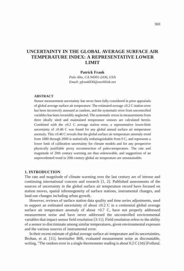
969

UNCERTAINTY IN THE GLOBAL AVERAGE SURFACE AIRTEMPERATURE INDEX: A REPRESENTATIVE LOWER

LIMIT

Patrick FrankPalo Alto, CA 94301-2436, USAEmail: [email protected]

ABSTRACTSensor measurement uncertainty has never been fully considered in prior appraisalsof global average surface air temperature. The estimated average ±0.2 C station errorhas been incorrectly assessed as random, and the systematic error from uncontrolledvariables has been invariably neglected. The systematic errors in measurements fromthree ideally sited and maintained temperature sensors are calculated herein.Combined with the ±0.2 C average station error, a representative lower-limituncertainty of ±0.46 C was found for any global annual surface air temperatureanomaly. This ±0.46 C reveals that the global surface air temperature anomaly trendfrom 1880 through 2000 is statistically indistinguishable from 0 C, and represents alower limit of calibration uncertainty for climate models and for any prospectivephysically justifiable proxy reconstruction of paleo-temperature. The rate andmagnitude of 20th century warming are thus unknowable, and suggestions of anunprecedented trend in 20th century global air temperature are unsustainable.

1. INTRODUCTIONThe rate and magnitude of climate warming over the last century are of intense andcontinuing international concern and research [1, 2]. Published assessments of thesources of uncertainty in the global surface air temperature record have focused onstation moves, spatial inhomogeneity of surface stations, instrumental changes, andland-use changes including urban growth.

However, reviews of surface station data quality and time series adjustments, usedto support an estimated uncertainty of about ±0.2 C in a centennial global averagesurface air temperature anomaly of about +0.7 C, have not properly addressedmeasurement noise and have never addressed the uncontrolled environmentalvariables that impact sensor field resolution [3-11]. Field resolution refers to the abilityof a sensor to discriminate among similar temperatures, given environmental exposureand the various sources of instrumental error.

In their recent estimate of global average surface air temperature and its uncertainties,Brohan, et al. [11], hereinafter B06, evaluated measurement noise as discountable,writing, "The random error in a single thermometer reading is about 0.2 C (1σ) [Folland,

et al., 2001] ([12]); the monthly average will be based on at least two readings a daythroughout the month, giving 60 or more values contributing to the mean. So the errorin the monthly average will be at most = 0.03 C and this will beuncorrelated with the value for any other station or the value for any other month."Paragraph [29] of B06 rationalizes this statistical approach by describing monthlysurface station temperature records as consisting of a constant mean plus weathernoise, thus, "The station temperature in each month during the normal period can beconsidered as the sum of two components: a constant station normal value (C) and arandom weather value (w, with standard deviation σi)." This description plus the useof a reduction in measurement noise together indicate a signal averagingstatistical approach to monthly temperature.

1.1. The scope of the studyThis study evaluates a lower limit to the uncertainty that is introduced into thetemperature record by the estimated noise error and the systematic error impacting thefield resolution of surface station sensors.

Basic signal averaging is introduced and then used to elucidate the meaning of theestimated ±0.2 C average uncertainty in surface station temperature measurements asdescribed by Folland, et al. [12]. An estimate of the noise uncertainty in any givenannual temperature anomaly is then developed. Following this, the lower limits ofsystematic error in three temperature sensors are calculated using previously reportedideal field studies [13].

Finally, the average measurement noise uncertainty and the lower limit ofsystematic error in a Maximum–Minimum Temperature System (MMTS) sensor arecombined into a total lower limit of uncertainty for an annual anomaly, referenced toa 30-year mean. The effect of this lower-limit uncertainty on the global averagesurface air temperature anomaly time series is described. The study ends with asummary and a brief discussion of the utility of the instrumental surface airtemperature record as a validation target in climate studies.

2. SIGNAL AVERAGINGThe error in an observable due to random noise can be made negligible by averagingrepetitive measurements [14, 15]; a technique that is exploited to excellent effect inspectroscopy [16]. Three cases below show when noise reduction by signal averagingis appropriate, and when it is not. The statistical model in B06 is then appraised in lightof these cases.

2.1. Case 1In signal-averaging repetitive measurements of a constant temperature, themeasurement in a random noise model is,

, (1)

where ti is the measured temperature, τc is the constant "true" temperature, and ni is the

t ni c i= +τ

1 60/

0 2 60. /

970 Energy & Environment · Vol. 21, No. 8, 2010

random noise associated with the ith measurement. When the noise is stationary, it has

a constant average intensity and a mean of 0. The mean temperature is ,

and the ‘mean temperature ± mean noise’ is,

. (2)

When N is large and the noise is stationary, and

, where σ 2n is the variance of the noise intensity, and "⇒" signifies

‘approaches equality with.’ Finally,

. (3)

That is, given a constant temperature and stationary random noise, averaging repetitive

measurements of any constant temperature reduces the impact of noise as , and

at large N, and [15, 17, p. 53ff]. Noise reduction by signal

averaging is thus entirely appropriate when data fall within Case 1.

2.2. Case 2Now suppose the conditions of Case 1 are changed so that the N true temperaturemagnitudes, τi, vary inherently but the noise variance remains stationary and of constantaverage intensity. Thus, , while .Then,

, (4)

where ti is again the measured temperature, τi is the "true" instantaneous temperature,and ni is again the noise intensity associated with the ith measurement. This case mayreflect a series of daily temperatures from any well-sited and maintained surfacestation sensor. In this case the ‘mean temperature ± mean noise’ will again be,

. (5)T nN

tN

n TN

i ii

N

i

Nn

_ _ _

( )± = ± = ±==∑∑1 1 2

11

σ

t ni i i= +τ

σ σ σ σ12 2 2 2= = = = =... ...i j nτ τ τ τ1 ≠ ≠ ≠ ≠ ≠... ...i j n

σ n N ⇒ 0T c

_

⇒ τ1 N

T nN

tN

N TN

i ni

Nn

_ _ _

± = ± = ±=∑1 1 2

1

σ σ

( )n Nii

N

n⇒=∑ 2

1

2σ

( )_

t Tii

N

− ==∑ 2

1

t T ni i− =_

T nN

tN

t Ti ii

N

i

N_ _ _

( )± = ± −==∑∑1 1 2

11

TN

tii

N_

==∑1

1

Uncertainty in the global average surface air temperature index: 971a representative lower limit

However, a further source of uncertainty now emerges from the condition .

The mean temperature, , will have an additional uncertainty, ±s, reflecting the fact

that the τi magnitudes are inherently different. The result is a scatter of the inherently

different temperature magnitudes about the mean, because now ,

where represents the difference between the "true" magnitude of τi and , apart

from noise. The magnitudes of the ni and the τi, are physically independent and

uncorrelated, and ni and are statistically independent. Therefore the uncertainties

due to these factors can be calculated separately:

, but [17,p. 9ff] (6)

The condition of noise stationarity means that the ni have a true constant mean of zero

(i.e., µnoise = 0). However, the second part of eqn. (6) shows that use of the empirical mean

temperature, , in calculating , removes a degree of freedom from s2.

Following from eqns. (5) and (6), although the impact of random noise on diminishes

with , the magnitude uncertainty in , given by, [17, p. 9ff],

does not.

For Case 2 measurements the noise variance, , and the magnitude uncertainty,

±s, must enter into the total uncertainty in the mean temperature as .Therefore under Case 2, the uncertainty never approaches zero no matter how large

N becomes, because although ±σn should automatically average away, ±s is neverzero.

The usual way to represent the uncertainty in averages of inherently varyingmagnitudes is with the standard deviation (SD) of the total scatter about the mean [17,

p. 11], e.g., . If the sensor ±σn has been measured

independently, then ±s can be extracted as becausemeasurement noise and magnitude scatter are statistically independent. The magnitudeuncertainty, ±s, is a measure of how well a mean represents the state of the system. Alarge ±s relative to a mean implies that the system is composed of stronglyheterogeneous sub-states poorly represented by the mean state [18]. This caution hasbearing on the physical significance of mean temperature anomalies (see below).

2.3. Case 3Finally, suppose a series of N temperature measurements of inherently uniquemagnitudes but now also with unique and unequal noise variances. Thus as in Case 2,

± = ±s SD Nn∓ ( )σ

SD t T Nii

N

= − −=∑ ( ) ( )

_2

1

1

T N sn

_

( )± ±σσ n

2

± =−

=∑

sN

ii

N

( )∆τ 2

1

1T_

1 N

T_

∆τ τi i T= −T_

sN i

i

N2 2

1

1

1=

− =∑ ( )∆τσ σ

noise ii

Nnoise

Nn

N2 2

1

1= → ±=∑ ( )

∆τ i

T_

∆τ i

( ) ( )t T ni i i− = + ∆τ

T_

τ τi j≠


, but now both and .This condition could arise from a time-dependent shift in the magnitude of themeasurement noise of a single sensor, or when averaging temperatures from multiplesensors that each exhibits an independent and unique noise variance. The lattersituation is closest to a real-world spatial average, in which temperature measurementsfrom numerous stations are combined.

2.3.1. Case 3aIf the unequal noise variances from each and all of the station sensors are known to be

stationary and uncorrelated, then and the variance of the mean is

[17, p. 57]. One can simplify analysis by scaling all the variances

to a single variance, thus , where

are the coefficients of scale. Each of the N unequal variances entering amean can now be transformed into an average variance of uniform magnitude as,

(7)

where , and is a constant stationaryvariance. On combining N measurements, the variance of the mean becomes,

(8)

The average noise uncertainty in is then , and if

σ 2i was the minimum of variances, then . Thus, with stationary noise variances

of known but uneven magnitude, an average noise uncertainty can be found,

, that again diminishes as . It is important to notice that

of Case 2, a variance of noise, is calculationally and conceptually distinct from of

Case 3, an average of variances.

2.3.2. Case 3bWhen sensor noise variances have not been measured and neither their stationarity northeir magnitudes are known, an adjudged average noise variance must be assignedusing physical reasoning [19]. For multiple sensors of unknown noise provenance, orfor a time series from a single sensor of unknown and possibly irregular variance, an

σ n2

σ n21 N± = ±σ σnoise cq

q > 1

T_

σ

σ σ

σµ2

21

2

211

1= = =

=∑ ( )

q

N

q

q

N

ci

n

c

c

σ σi c2 2≡q N c c cj k n= × + + + +( ) ( ... )1 1

1 112 2 2 2

Nc c c

Nc c ci j i k i n i j k n( ... ) ( ...σ σ σ σ+ + + + = + + + + ))σ σ σi i cq q2 2 2= =

c c cj k n, , ...,

σ σ σ σ σ σ σ σi i j j i k k i n n ic c c2 2 2 2 2 2 2 2= = = =; ; ; ...;

σ σµ2 2

1

1 1==∑ ( )ii

n

TN

tii

N_

==∑1

1

σ σ σ σ12 2 2 2≠ ≠ ≠ ≠ ≠... ...i j n

τ τ τ τ1 ≠ ≠ ≠ ≠ ≠... ...i j nt ni i i= +τ


adjudged estimate of measurement noise variance is implicitly a simple average,

, where each is of unknown provenance and nominally represents

the unique noise variance of one of the N measurements. The primed sigma indicatesan adjudged estimate and distinguishes Case 3b noise uncertainty from those of Cases1-3a.

In the case of an adjudged average noise uncertainty, each temperaturemeasurement must be appended with the constant uncertainty estimate as, .

The mean of a series of N measurements is the usual , but the average

noise uncertainty in the measurement mean is [17, p. 58,wi = 1], with one degree of freedom lost because the estimated noise variance in eachmeasurement is an implied mean.

Thus when calculating a measurement mean of temperatures appended with anadjudged constant average uncertainty, the uncertainty does not diminish as .Under Case 3b, the lack of knowledge concerning the stationarity and true magnitudesof the measurement noise variances is properly reflected in a greater uncertainty in themeasurement mean. The estimated average uncertainty in the measurement mean,

, is not the mean of a normal distribution of variances, because under Case 3b themagnitude distribution of sensor variances is not known to be normal.

The condition in Case 3 also produces a magnitude uncertainty, ±s, inanalogy with Case 2. When the magnitudes and stationarities of measurement noisevariances are both unknown, the total uncertainty in a measurement mean is

. In Case 3b, does not diminish as , and ±s–

cannot be separated from .

3. RESULTS AND DISCUSSION3.1. The average noise uncertainty estimateIt is now possible to evaluate the ±0.2 C uncertainty estimate of Folland, et al. [12],who "estimated the two standard error (2σ) measurement error to be 0.4 °C in anysingle daily [land air-surface temperature] observation." This estimate was not basedon a survey of sensors nor followed by a supporting citation. The temperature sensorat each station will exhibit a unique and independent noise variance, and the contextin Ref. [12] provides that the ±0.2 C is from the estimated average variance of theensemble of variances of the individual surface station sensors entering measurementsinto a global average surface air temperature. This estimated uncertainty thus fallsunder Case 3, above.

Following this identification, the question next becomes whether the relevantstation sensor noise variances are stationary and of known magnitude. In general,detailed examinations of errors in station histories have focused principally oninhomogeneities due to instrumental changes and station moves [3, 9, 20-24], but have

± ′σ µ

1 N± ′σ µ± = − −=∑σ total ii

N

t T N( ) ( )_

2

1

1

τ τi j≠

± ′σ µ

1 N

± ′ = × ′ −σ σµ N Nnoise2 1( )

TN

tii

N_

==∑1

1

ti noise± ′σ

′σ i2′ = ′

=∑σ σnoise ii

N

N2 2

1

1


not mentioned appraisals of station sensor variance. Reviews of time series qualitycontrol and homogeneity adjustments do not discuss sensor evaluation [7-10], and themethodological report of USHCN data quality [25] does not describe validation orsampling of noise stationarity in temperature sensors. The surface station sensordiagnostics, available in the online reports of the new USCRN National Climatic DataCenter network, include standard deviations calculated from the twelve temperaturesrecorded hourly (http://www.ncdc.noaa.gov/crn/report; see the "Air TemperatureSensor Summary," under "Instruments"). But despite the set of ~8640 monthlystandard deviations from individual CRN sensor data streams, which should give somemeasure of the magnitude and stationarity of variance, no extensive survey of stationsensor variance is evident in published work.

The quality of individual surface stations is perhaps best surveyed in the US by wayof the commendably excellent independent evaluations carried out by Anthony Wattsand his corps of volunteers, publicly archived at http://www.surfacestations.org/ andapproaching in extent the entire USHCN surface station network. As of this writing,69% of the USHCN stations were reported to merit a site rating of poor, and a further20% only fair [26]. These and more limited published surveys of station deficits [24,27-30] have indicated far from ideal conditions governing surface stationmeasurements in the US. In Europe, a recent wide-area analysis of station seriesquality under the European Climate Assessment [31], did not cite any survey ofindividual sensor variance stationarity, and observed that, "it cannot yet be guaranteedthat every temperature and precipitation series in the December 2001 version will besufficiently homogeneous in terms of daily mean and variance for every application."Likewise, sensor variance was not mentioned in recent studies of data quality fromsurface stations in Canada [32, 33], where it was noted in 2002 that, "adjustments haveonly been carried out for identified step changes and the homogenized monthlytemperatures have not been adjusted for artificial trends at this time." The authorsstated further that, "The preferred methodology would be to develop procedures basedon each cause of inhomogeneity. However, this would be a very site-specific task thatwould be nearly impossible to implement on a Canada-wide basis." Stationevaluations for sensor variance are also not mentioned in the climate normals report ofEnvironment Canada [34].

Thus, there apparently has never been a survey of temperature sensor noisevariance or stationarity for the stations entering measurements into a globalinstrumental average, and stations that have been independently surveyed haveexhibited predominantly poor site quality. Finally, Lin and Hubbard have shown [35]that variable field conditions impose non-linear systematic effects on the response ofsensor electronics, suggestive of likely non-stationary noise variances within thetemperature time series of individual surface stations (see Section 3.2.2).

These considerations indicate that an assumption of stationary noise variance intemperature time series cannot be presently justified, and that the assumption ofrandom station errors is not empirically tenable. Therefore, the ±0.2 C estimate in Ref.[12] is the assessed of Case 3b above, namely an adjudged assignment takento represent the average uncertainty from an ensemble of surface station measurement

± ′σ noise


noise variances of unknown magnitude and stationarity. It does not represent themagnitude of random noise for any specific measurement, nor does it represent thenoise variance of any specific sensor, nor is it an average of known stationaryvariances. Following Case 3b, the ±0.2 C estimate of Ref. [12] is ; an adjudgedconstant average uncertainty that attaches to each surface temperature measurementand that must therefore be carried into a spatial average of N station measurements as

. This uncertainty does not decrement as when calculating a mean, and will constitute a significant part of the total uncertaintyin any global average surface air temperature index. Therefore the noisereduction model in B06 is in error.

Clearly, a different statistical approach to uncertainty in air temperature averages iswarranted; one that reflects the true empirical uncertainties. This approach is shown next.

3.2. An empirical approach to temperature uncertaintyTmax and Tmin are typically measured many hours apart under physically opposingirradiance conditions. Although they may have an identical instrumental noisestructure, they are experimentally independent measurements of physically differentobservables, each measured separately.

3.2.1. Uncertainty due to estimated noiseFollowing from Case 3b and the discussion in Section 3.1 above, the estimated per-measurement uncertainty = ±0.2 C from Ref. [12] must enter as a constantapplied to each temperature measurement. This value also represents the achievableuncertainty recommended by the World Meteorological Organization [36]. Using thisvalue, and including normalization to a 30-year mean, the noise uncertainty in anannual anomaly is now stepwise calculated.

In order to maximally reduce the uncertainty, the annual temperature and the 30-yearmean temperature were calculated directly, as though from individual

measurements, as , where is annual mean temperature, is a 30-year

mean reference, ti is an individual measurement, and N is the number of measurements(twice the number of days entering each mean). Applying the estimated average per-measurement uncertainty, , the total noise uncertainty in anymeasurement average is

(9)

where N is the number of measurements entering the mean. This calculation yields= ±0.200 for both an annual mean temperature and a 30-year mean, and this

uncertainty enters separately into each mean. In calculating the uncertainty in an annual anomaly referenced against a multi-

decadal mean, , the uncertainties in each mean value are combined in∆T T Ta = − ˆ

± ′�σ n

± ′ = × ′−

�σ σ

nnN

N

2

1

± ′ = ±σ n C0 2.

T̂T_

T or TN

tii

N

ˆ ==∑1

1

± ′σ n

1 N

1 N± ′σ µ± ′ = × ′ −σ σµ N Nnoise2 1( )

± ′σ noise


quadrature [17, p. 48]. The average noise uncertainty in the annual anomaly is then,

= ±0.283 C, where , arethe average noise uncertainties in the annual mean temperature, or the 30-year meantemperature, respectively. The represents the minimal noise-derived uncertaintyin an annual temperature anomaly, referenced to a 30-year mean, for any given surfacestation when using the per-measurement estimated = ±0.20 C of Folland, et al. [12].

It is also possible to obtain an annual anomaly by normalizing an annualtemperature series to a fitted mean obtained by regression against a 30-year annualtemperature time series. However, a regression mean introduces the uncertainty of thefit into the total uncertainty. This new uncertainty is the numerical estimated standarddeviation (e.s.d.) of the fit, further scaled to reflect the reduced degrees of freedominduced by autocorrelation of the residuals [37]. The average uncertainty of eachannual anomaly magnitude is then,

, (10)

where (e.s.d.)i is the numerical estimated standard deviation per point, N is the numberof points, and ν is the number of degrees of freedom lost through autocorrelation ofthe residuals.

Finally, in every case, a magnitude uncertainty, ±s, must also be included as part of

the uncertainty in an annual anomaly. The magnitude uncertainty in an annual

anomaly, ±sa, can be estimated as , where ±s is the magnitude

uncertainty in a yearly average temperature, is the average annual temperature

anomaly, referenced to a 30-year mean, and is the average temperature for that

same year. This uncertainty transmits the confidence that may be placed in an anomaly

as representative of the state of the system.

3.2.2. Uncertainty due to systematic impacts on instrumental field resolutionThe degraded instrumental resolution due to the systematic error from uncontrolledvariables [38, 39] has apparently never found its way into any published assessmentof the uncertainties in the global average surface air temperature index. The systematicmeasurement errors originating from the field exposure of the Min-Max TemperatureSystem (MMTS), Automated Surface Observing System (ASOS), the Gill shield, andother commonly used electronic temperature sensors and shields have beeninvestigated in excellent detail by Lin and Hubbard [35] and found to originateprincipally from solar radiation loading and wind speed effects. Other sources of errorwere enumerated as, "originating with the sensing element, analog signalconditioning, and data acquisition system [and] include the sensor interchangeabilityerror, polynomial and linearization errors, self-heating error, voltage or currentreference (excitation) error, total offset and drift in the amplifiers and ADC (associated

T_

∆Ta

± = ± ×s s T Ta a( )∆

± ′ = ′ + × −ˆ ( ) [ ( . . .) ( )]σ σ ν�

nT

iN e s d N2 2

′σ n

± ′σ̂ n

± ′�σ n

T̂± ′�σ n

T± ′ = ′ + ′ = +ˆ ( ) ( ) ( . ) ( . )ˆσ σ σn n

Tn

T C C� �2 2 2 20 2 0 2


with stability), and lead wire error." All these systematic errors, including themicroclimatic effects, vary erratically in time and space [40-45], and can impose non-stationary and unpredictable biases and errors in sensor temperature measurementsand data sets. These uncontrolled experimental variables degrade instrumental fieldresolution, and must be included in assessments of uncertainty in spatially andchronologically averaged temperatures.

Under ideal site conditions Hubbard and Lin recorded thousands of air

temperatures using MMTS, ASOS, Gill, and other sensors and shields [13, 35, 42],

and compared them to temperatures simultaneously measured using a calibrated high-

resolution R. M. Young temperature probe with an aspirated shield. For each recorded

temperature, the measurement rate was 6 min.-1 integrated across 5 min., reducing the

random noise in each aggregated temperature measurement by . The

temperature data thus consisted primarily of a bias and a resolution width relative to

the "true" temperature provided by the R. M. Young probe. Figure 1 shows the ideal

day time field resolution envelopes of the MMTS, ASOS temperature sensors and Gill

shield [13], fitted with the Gaussian ,

where a is a vertical offset, b is an intensity scaler, σ is the Gaussian (intensity)/e1/2

half-width (the standard deviation), and µ is the Gaussian mean. The results of the fits

are shown in Table 1. Analogous fits to the 24-hour average data yielded, (sensor, µ (C), 1σ (±C), r2):

MMTS, (0.29, 0.25, 0.995); ASOS, (0.18, 0.14, 0.993), and; Gill, (0.21, 0.19, 0.979).These values are somewhat different from those originally reported in Ref. [13], whichwere not obtained from Gaussian fits.

The sensor evaluations were carried out under conditions of ideal siting andexcellent maintenance [13]. Therefore, the field resolutions listed above approximatebest achievable values and represent an attainable lower limit of instrumentalresolution under field use conditions. Instrumental resolution by itself constitutes theminimum uncertainty in any temperature measurement, and the response of ideallysited and maintained sensors provides an empirical lower limit of field resolution.

Table 1: Lower Limit Temperature Sensor Resolutions from Gaussian fits

a b x+ × − −( ) exp{ [( )( ) ]}1 2 1 2 2σ π µ σ

1 30/


Figure 1. Daytime (a) and nighttime (b) resolution of: (o), MMTS; (�), ASOS, and;(∆) Gill temperature sensors. The points were derived from Figure 2a,b of Ref. [13],using the program Digitizeit (www.digitizeit.de). The curves were normalized to unit

area and each temperature bias relative to the R. M. Young probe was removed toyield a common mean of 0 C. The lines are Gaussian fits to the points. The ASOS

and Gill data were vertically shifted 1 and 2 units, respectively, for clarity.

Temperature sensor resolution can, however, be significantly improved by applicationof a real-time empirical filtering algorithm to minimize the systematic error due touncontrolled micro-climate variables [13, 46], as shown in Figure 2.


From the fits in Figure 2, the improved resolution of filtered MMTS data yields an

uncertainty of ±0.093 C in daily mean temperature (cf. Figure 2, Legend). Using the

equations gathered in Table 2, a minimum adjudged average ±0.1 C noise uncertainty

and the ±0.093 C filtered resolution from a well-maintained MMTS sensor in an ideal

site location, alone, yield a r.m.s. uncertainty in a per-station yearly temperature

anomaly of = ±0.193 C. However, the field resolution of

surface station temperature sensors is not yet commonly improved using the Hubbard-

Lin filter.

Figure 2. Gaussian fits to algorithmically filtered MMTS temperature resolutiondata, digitized as in Figure 4 and extracted from Ref. [46]. a. Daytime and b.

nighttime, normalized to unit area and with the temperature bias again removed toproduce a common mean of 0 C. The fit parameters are: a. σ = ±0.093±0.002 C,

r2 = 0.993, and; b. σ = ±0.029±0.001 C, r2 = 0.987.

( . ) ( . )0 141 0 1322 2+


3.2.3. The lower limit uncertainty in an annual temperature anomalyAppropriate statistics are now used to combine the average noise uncertainty ofSection 3.2.1 and the ideal lower limit of systematic error from Section 3.2.2, into acomposite lower limit of measurement uncertainty in surface station air temperatureanomalies.

The equations used to propagate an appended per-measurement uncertainty into anannual anomaly, due to the entry of systematic error into field resolution, areanalogous to those used to propagate the constant average noise uncertainty. Onedegree of freedom is lost in the statistical uncertainty mean because everydetermination of systematic error in a temperature data set is an average of the effectsof uncontrolled variables. Each determination of field resolution uncertainty is alsounique in terms of bias and width, because uncontrolled variables fluctuate in time andspace. The idealized field resolutions for MMTS, ASOS sensors and the Gill shieldreferenced to a 30-year mean are shown in Table 2. For an MMTS sensor under idealsite conditions these equations yielded ±σ–r = ±0.36 C, which represents a lower limitof resolution uncertainty from each such station entering into a global averageanomaly. Table 2 also includes the analogous Case 3b average noise uncertainties fromSection 3.2.1.

Table 2: Uncertainty in an Annual Anomaly Due to Noise or Resolutiona

a. Rows are, top: uncertainty in a yearly mean temperature; bottom: uncertainty in yearly anomalyreferenced to a 30 year mean. b. Uncertainty Equation. c. 1σ (±C; day, night): MMTS=(0.23, 0.17);ASOS=(0.16, 0.11), and Gill=(0.22, 0.12); see Table 1.

Figure 1 and Table 2 reflect average noise, and the resolution uncertainties currentlyexpected from the ideal placement and maintenance of conventional surface stationtemperature sensors. For any one surface-station deploying a modern MMTS sensor,the minimal measurement uncertainty will be the average noise plus the idealresolution uncertainties combined in quadrature [39, Section 5, 47]. From Table 2, foran MMTS sensor the total noise plus resolution lower-limit 1σ measurementuncertainty in an annual temperature anomaly referenced to a 30-year mean is

= ±0.46 C.The meaning of an ideal lower limit of measurement uncertainty provides that it is

of lower magnitude than the uncertainty in each and all of the other homologoussingle-station measurements, worldwide. Thus, liquid-in-glass (LIG) thermometers in

± = +ˆ ( . ) ( . )σ 0 283 0 3592 2


Cotton Regional Shelters are reckoned to be of lower field resolution than the MMTSsensor [3, 41, 48]. Further, precision comparisons have shown that the systematic errorintroduced into surface station temperatures by the Cotton Regional Shelter is abouttwice that of the MMTS aspirated shield [42]. Thus, the ±0.46 C lower limituncertainty of a modern MMTS sensor underestimates the uncertainty in themeasurements from LIG thermometers in CRS shields that constitute the bulk of the20th century global surface air temperature record.

The ±0.46 C lower limit of MMTS uncertainty is therefore applicable to everymeasurement in the global land surface record, because of the very high likelihood thatit is of lower magnitude than the unknown uncertainties produced by surface stationsensors that are generally more poorly maintained, more poorly sited, and less accuratethan the reference sensors. The ideal resolutions of Figure 1 and Table 2 thus providerealistic lower-limits for the air temperature uncertainty in each annual anomaly ofeach of the surface climate stations used in a global air temperature average. Thislower limit of measurement uncertainty for each surface station annual temperatureanomaly is propagated into a global average as,

, (11)

to produce the total lower limit of uncertainty in a global temperature anomaly. Here

σ∧ 2

i is the lower limit mean noise plus resolution annual temperature uncertainty at the

ith station, and N is the number of stations. For example, the lower limit of sensor

uncertainty propagates into a global surface average air temperature anomaly as

, when, e.g., N = 4349 as in Ref. [11].

This uncertainty enters each anomaly in a global annual time series, and will be in

addition to the commonly discussed uncertainties resulting from weather noise, step

discontinuities, incomplete station coverage, land-use changes, siting artifacts [26],

and albedo changes [49]. It seems likely that the new USCRN stations [50] will not

significantly improve on the lower limit uncertainty any time soon [51].

3.2.4. The representative lower limit uncertainty in a global average air temperatureanomaly time seriesIn independent calculations of global average surface air temperature anomalies,[52-54], the major source of uncertainty was assigned to incomplete stationcoverage, 2σ = ±0.07 C [55], with most of the remaining uncertainty assigned tothe temporal inhomogeneity of temperature records [5]. These estimates of the globalsurface air temperature index did not include the instrumental uncertainties present inthe surface station temperature measurements themselves, however. Therefore, theeffect of the ideal lower limit uncertainty illustrated above on the reliability of theglobal average surface air temperature index is briefly considered below.

± = ± × − = ±σ global N C N C( . ) ( ) . 0 46 1 0 462

± =−

=∑

ˆˆ

σσ

total

ii

N

N

2

1

1


The uncertainties due to average noise and instrumental resolution in maritimetemperature sensors remain to be evaluated and propagated into marine airtemperature anomalies [11]. However, assessments of instrumental uncertainties inmarine air and sea-surface temperatures have revealed evidence of significantly largesystematic errors [56, 57], which both bias marine temperature measurements andimply an instrumental resolution degraded by uncontrolled environmental variablesthroughout the 20th century. Uncertainties in marine temperatures are thus not likelyto be less than appraised here for land surface stations [4, 58, 59]. Therefore, the lowerlimit uncertainty in an MMTS land surface anomaly, σ = ±0.46 C , can be crediblyapplied to the global land + ocean anomalies.

Figure 3 shows the global average surface air temperature anomaly index ascompiled from surface and maritime meteorological stations and provided by theGoddard Institute for Space Studies, as updated on 18 February 2010. The lower limit±0.46 C uncertainty in an annual surface anomaly is plotted on Figure 3 to illustrate acredible lower limit of uncertainty in the current surface air temperature anomalyseries.

Figure 3. (•), the global surface air temperature anomaly series through 2009, asupdated on 18 February 2010, (http://data.giss.nasa.gov/gistemp/graphs/). The grey

error bars show the annual anomaly lower-limit uncertainty of ±0.46 C.


Figure 3 shows that the trend in averaged global surface air temperature from 1880through 2000 is statistically indistinguishable from zero (0) Celsius at the 1σ levelwhen this lower limit uncertainty is included, and likewise indistinguishable at the 2σlevel through 2009. Thus, although Earth climate has unambiguously warmed duringthe 20th century, as evidenced by, e.g., the poleward migration of the northern tree line[60-62], the rate and magnitude of the average centennial warming are not knowable.

4. SUMMARY AND CONCLUSIONSThe assumption of global air temperature sensor noise stationarity is empirically

untested and unverified. Estimated noise uncertainty propagates as ,

rather than as . Future noise uncertainty in monthly means would greatlydiminish if the siting of surface stations is improved and the sensor noise variancesbecome known, monitored, and empirically verified as stationary.

The persistent uncertainty due to the effect of uncontrolled microclimatic variableson temperature sensor resolution has, until now, never been included in publishedassessments of global average surface air temperature. Average measurement noiseand the lower limit of systematic sensor errors combined to yield a representativelower limit uncertainty of ±0.46 C in a 30-year mean annual temperature anomaly. Inview of the problematic siting record of USHCN sensors, a globally completeassessment of current air temperature sensor field resolution seems likely to reveal ameasurement uncertainty exceeding ±0.46 C by at least a factor of 2.

The ±0.46 C lower limit of uncertainty shows that between 1880 and 2000, thetrend in averaged global surface air temperature anomalies is statisticallyindistinguishable from 0 C at the 1σ level. One cannot, therefore, avoid the conclusionthat it is presently impossible to quantify the warming trend in global climate since1880.

Finally, the relatively large uncertainty attending the global surface instrumentalrecord means that the centennial temperature trend is not a precision target forvalidation tests of climate models. Likewise, the current surface instrumental recordcannot credibly be used to train or renormalize any physically valid proxyreconstruction of paleo-temperature with sufficient precision to resolve anytemperature difference less than at least 1 C, to 95% confidence. It is thus impossibleto know whether the rate of warming during the 20th century was climatologicallyunprecedented, or to know the differential magnitude of any air temperature warmeror cooler than the present, within ±1 C, for any year prior to the satellite era. Thereforeprevious suggestions, that the rate or magnitude of present climate warming is recentlyor millennially unprecedented, must be vacated.

ACKNOWLEDGEMENTSThe author thanks Prof. David Legates, University of Delaware, Dr. David Stockwell,University of California San Diego, and Prof. Demetris Koutsoyiannis, AthensNTUA, for critically reviewing a previous version of this manuscript.

±σ n N

± ′ −N Nnσ 2 1( )


REFERENCES1. Cicerone, R., Barron, E.J., Dickenson, R.E., Fung, I.Y., Hansen, J.E., Karl, T.R., Lindzen,

R.S., McWilliams, J.C., Rowland, F.S., Sarachik, E.S. and Wallace, J.M., Climate ChangeScience: An Analysis of Some Key Questions, The National Academy of Sciences, USA,http://books.nap.edu/openbook.php?record_id=10139&page=1, Last accessed on: 28March 2010.

2. Bernstein, L., Bosch, P., Canziani, O., Chen, Z., Christ, R., Davidson, O., Hare, W., Huq,S., Karoly, D., Kattsov, V., Kundzewicz, V., Liu, J., Lohmann, U., Manning, M., Matsuno,T., Menne, B., Metz, B., Mirza, M., Nicholls, N., Nurse, L., Pachauri, R., Palutikof, J.,Parry, M., Qin, D., Ravindranath, N., Reisinger, A., Ren, J., Riahi, K., Rosenzweig, C.,Rusticucci, M., Schneider, S., Sokona, Y., Solomon, S., Stott, P., Stouffer, R., Sugiyama,T., Swart, R., Tirpak, D., Vogel, C. and Yohe, G., Climate Change 2007: Synthesis Report.Contribution of Working Groups I, II and III to the Fourth Assessment Report of theIntergovernmental Panel on Climate Change, in, Pachauri, R.K. & Reisinger, A., eds.IPCC, Geneva, Switzerland, 2007, pp. 104 pp.

3. Karl, T.R., Tarpley, J.D., Quayle, R.G., Diaz, H.F., Robinson, D.A. and Bradley, R.S., TheRecent Climate Record: What it Can and Cannot Tell Us, Rev. Geophys., 1989, 27(3),405-430.

4. Trenberth, K.E., Christy, J.R. and Hurrell, J.W., Monitoring Global Monthly MeanSurface Temperatures, J. Climate, 1992, 5, 1405-1423; doi: 10.1175/1520-0442(1992)005.

5. Hansen, J. and Lebedeff, S., Global Trends of Measured Surface Air Temperature, J.Geophys. Res., 1987, 92(D11), 13345-13372.

6. Easterling, D.R., Peterson, T.C. and Karl, T.R., On the Development and Use ofHomogenized Climate Datasets, J. Climate, 1996, 9(6), 1429-1434; doi: 10.1175/1520-0442(1996)009<1429:OTDAUO>2.0.CO;2.

7. Jones, P.D., Osborn, T.J. and Briffa, K.R., Estimating Sampling Errors in Large-ScaleTemperature Averages, J. Climate, 1997, 10(10), 2548-2568; doi: 10.1175/1520-0442(1997)010<2548:ESEILS>2.0.CO;2.

8. Peterson, T.C., Easterling, D.R., Karl, T.R., Groisman, P., Nicholls, N., Plummer, N.,Torok, S., Auer, I., Boehm, R., Gullet, D., Vincent, L., Heino, R.T., H., Mestre, O.,Szentimrey, T., Salinger, J., Førland, E., Hanssen-Bauer, I., Alexandersson, H., Jones, P.and Parker, D., Homogeneity adjustments of in situ atmospheric climate data: a review,Int. J. Climatol., 1998, 18(13), 1493-1517.

9. Peterson, T.C., Vose, R., Schmoyer, R. and Razuvaëv, V., Global historical climatologynetwork (GHCN) quality control of monthly temperature data, Int. J. Climatol., 1998,18(11), 1169-1179; doi: 10.1002/(SICI)1097-0088(199809)18:11<1169::AID-JOC309>3.0.CO;2-U.

10. Peterson, T.C. and Sun, B., Estimating temperature normals for USHCN stations, Int. J.Climatol., 2005, 25(4), 1809-1817; doi: 10.1002/joc.1220.


11. Brohan, P., Kennedy, J.J., Harris, I., Tett, S.F.B. and Jones, P.D., Uncertainty estimates inregional and global observed temperature changes: A new data set from 1850, J. Geophys.Res., 2006, 111 D12106 1-21; doi:10.1029/2005JD006548; see http://www.cru.uea.ac.uk/cru/info/warming/.

12. Folland, C.K., Rayner, N.A., Brown, S.J., Smith, T.M., Shen, S.S.P., Parker, D.E.,Macadam, I., Jones, P.D., Jones, R.N., Nicholls, N. and Sexton, D.M.H., GlobalTemperature Change and its Uncertainties Since 1861, Geophys. Res. Lett., 2001, 28(13),2621-2624.

13. Hubbard, K.G. and Lin, X., Realtime data filtering models for air temperaturemeasurements, Geophys. Res. Lett., 2002, 29(10), 1425 1-4; doi: 10.1029/2001GL013191.

14. Aunon, J.I., McGillum, C.D. and Childers, D.G., Signal Processing in Evoked PotentialResearch: Averaging and Modeling, CRC Crit. Rev. Bioeng., 1981, 5(4), 323-367; cf. eqs.10-18.

15. Leski, J., New Concept of Signal Averaging in the Time Domain, in, Nagel, J.H. & Smith,W.M., eds. Vol. 13: Proc. Annu. Int. Conf. IEEE Eng. Med. Biol. Soc., IEEE, Orlando,FL, 1991, pp. 367-369.

16. Mark, H. and Workman jr., J., Statistics in Spectroscopy, 2nd edn., Elsevier; cf. Chapter11, Amsterdam 2003.

17. Bevington, P.R. and Robinson, D.K., Data Reduction and Error Analysis for the PhysicalSciences, 3rd edn., McGraw-Hill, Boston 2003.

18. Esper, J. and Frank, D., The IPCC on a heterogeneous Medieval Warm Period, ClimaticChange, 2009, 94 267-273; doi: 10.1007/s10584-008-9492-z.

19. Gleser, L.J., Assessing uncertainty in measurement, Statist. Sci., 1998, 13 (3), 277-290;doi: 10.1214/ss/1028905888.

20. Guttman, N.B. and Plantico, M.S., Climatic Temperature Trends, J. Clim. Appl.Meteorol., 1987, 26 1428-1435; doi: 10.1175/1520-0450(1987)026<1428:CTN>2.0.CO;2.

21. Reek, T., Doty, S.R. and Owen, T.W., A Deterministic Approach to the Validation ofHistorical Daily Temperature and Precipitation Data from the Cooperative Network, Bull.Amer. Met. Soc., 1992, 73(6), 753-762; doi:10.1175/1520-0477(1992)073<0753:ADATTV>2.0.CO;2.

22. Easterling, D.R. and Peterson, T.C., A new method for detecting undocumenteddiscontinuities in climatological time series, Int. J. Climatol., 1995, 15 (4), 369-377; doi:10.1002/joc.3370150403.

23. Sun, B. and Peterson, T.C., Estimating temperature normals for USCRN stations, Int. J.Climatol., 2005, 25(14), 1809-1817; doi: 10.1002/joc.1220.

24. Pielke Sr., R., Nielsen-Gammon, J., Davey, C., Angel, J., Bliss, O., Doesken, N., Cai, M.,Fall, S., Niyogi, D., Gallo, K., Hale, R., Hubbard, K.G., Lin, X., Li, H. and Raman, S.,Documentation of Uncertainties and Biases Associated with Surface TemperatureMeasurement Sites for Climate Change Assessment, Bull. Amer. Met. Soc., 2007, 913-928; doi: 10.1175/BAMS-88-6-913.


25. NCDC, Environmental Information Summaries C-23; United States Climate Normals,1971-2000 Inhomogeneity Adjustment Methodology, National Climatic DataCenter/NESDIS/NOAA, http://lwf.ncdc.noaa.gov/oa/climate/normals/normnws0320.pdf,Last accessed on: 28 March 2010.

26. Watts, A., Is the U.S. Surface Temperature Record Reliable?, The Heartland Institute,Chicago, IL 2009

27. Davey, C.A. and Pielke Sr., R.A., Microclimate Exposures of Surface-Based WeatherStations, Bull. Amer. Met. Soc., 2005, 86(4), 497-504; doi: 10.1175/BAMS-86-4-497.

28. Runnalls, K.E. and Oke, T.R., A Technique to Detect Microclimatic Inhomogeneities inHistorical Records of Screen-Level Air Temperature, J. Climate, 2006, 19(6), 959-978.

29. Pielke Sr., R.A., Davey, C.A., Niyogi, D., Fall, S., Steinweg-Woods, J., Hubbard, K., Lin,X., Cai, M., Lim, Y.-K., Li, H., Nielsen-Gammon, J., Gallo, K., Hale, R., Mahmood, R.,Foster, S., McNider, R.T. and Blanken, P., Unresolved issues with the assessment ofmultidecadal global land surface temperature trends, J. Geophys. Res., 2007, 112 D24S081-26; doi: 10.1029/2006JD008229.

30. Fiebrich, C.A. and Crawford, K.C., Automation: A Step Toward Improving the Qualityof Daily Temperature Data Produced by Climate Observing Networks, Journal ofAtmospheric and Oceanic Technology, 2009, 26(7), 1246-1260.

31. Klein Tank, A.M.G., Wijngaard, J.B., Können, G.P., Böhm, R., Demarée, G., Gocheva,A., Mileta, M., Pashiardis, S., Hejkrlik, L., Kern-Hansen, C., Heino, R., Bessemoulin, P.,Müller-Westermeier, G., Tzanakou, M., Szalai, S., Pálsdóttir, T., Fitzgerald, D., Rubin, S.,Capaldo, M., Maugeri, M., Leitass, A., Bukantis, A., Aberfeld, R., van Engelen, A.F.V.,Forland, E., Mietus, M., Coelho, F., Mares, C., Razuvaev, V., Nieplova, E., Cegnar, T.,Antonio López, J., Dahlström, B., Moberg, A., Kirchhofer, W., Ceylan, A., Pachaliuk, O.,Alexander, L.V. and Petrovic, P., Daily dataset of 20th-century surface air temperatureand precipitation series for the European Climate Assessment, Int. J. Climatol., 2002,22(12), 1441-1453; doi: 10.1002/joc.773.

32. Vincent, L.A. and Gullett, D.W., Canadian historical and homogeneous temperaturedatasets for climate change analyses, Int. J. Climatol., 1999, 19(12), 1375-1388.

33. Vincent, L.A., Zhang, X., Bonsal, B.R. and Hogg, W.D., Homogenization of DailyTemperatures over Canada, J. Climate, 2002, 15 (11), 1322-1334; doi: 10.1175/1520-0442(2002)015<1322:HODTOC>2.0.CO;2.

34. Allsop, D. and Morris, R., Calculation of the 1971 to 2000 Climate Normals for Canada,Meteorological Service of Canada, http://www.climate.weatheroffice.ec.gc.ca/prods_servs/normals_documentation_e.html,Last accessed on: 28 March 2010.

35. Lin, X. and Hubbard, K.G., Sensor and Electronic Biases/Errors in Air TemperatureMeasurements in Common Weather Station Networks, J. Atmos. Ocean. Technol., 2004,21 1025-1032.

36. Rüedi, I., WMO Guide to Meteorological Instruments and Methods of Observation:WMO-8 Part I: Measurement of Meteorological Variables, 7th Ed., Chapter 1, WorldMeteorological Organization, Geneva 2006 http://www.wmo.int/pages/prog/www/IMOP/IMOP-home.html.


37. Santer, B.D., Wigley, T.M.L., Boyle, J.S., Gaffen, D.J., Hnilo, J.J., Nychka, D., Parker,D.E. and Taylor, K.E., Statistical significance of trends and trend differences in layer-average atmospheric temperature time series, J. Geophys. Res., 2000, 105(D6), 7337-7356.

38. Eisenhart, C., Expression of the Uncertainties of Final Results, Science, 1968, 160 1201-1204.

39. Taylor, B.N. and Kuyatt., C.E., Guidelines for Evaluating and Expressing the Uncertaintyof NIST Measurement Results, National Institute of Standards and Technology,Washington, DC 1994 http://www.nist.gov/pml/pubs/tn1297/index.cfm.

40. Ishida, H., Seasonal variations of spectra of wind speed and air temperature in themesoscale frequency range Boundary-Layer Meteorology, 1990, 52(4), 335-348.

41. Wendland, W.M. and Armstrong, W., Comparison of Maximum-Minimum Resistanceand Liquid-in-Glass Thermometer Records, J. Atmos. Oceanic Technol., 1993, 10(2),233-237.

42. Hubbard, K.G., Lin, X. and Walter-Shea, E.A., The Effectiveness of the ASOS, MMTS,Gill, and CRS Air Temperature Radiation Shields, J. Atmos. Oceanic Technol., 2001,18(6), 851-864.

43. Snyder, R.L., Spano, D., Duce, P. and Cesaraccio, C., Temperature data for phenologicalmodels, Int. J. Biometeorol., 2001, 45(4), 178-183.

44. Lin, X., Hubbard, K.G. and Meyer, G.E., Airflow Characteristics of Commonly UsedTemperature Radiation Shields, J. Atmos. Oceanic Technol., 2001, 18 (3), 329-339.

45. Tarara, J.M. and Hoheisel, G.-A., Low-cost Shielding to Minimize Radiation Errors ofTemperature Sensors in the Field, Hort. Sci., 2007, 42(6), 1372-1379.

46. Hubbard, K.G., Lin, X., Baker, C.B. and Sun, B., Air Temperature Comparison betweenthe MMTS and the USCRN Temperature Systems, J. Atmos. Ocean. Technol., 2004, 211590-1597.

47. Lira, I.H. and Wöger, W., The evaluation of standard uncertainty in the presence oflimited resolution of indicating devices, Meas. Sci. Technol., 1997, 8 441-443; doi:10.1088/0957-0233/8/4/012.

48. Quayle, R.G., Easterling, D.R., Karl, T.R. and Hughes, P.Y., Effects of RecentThermometer Changes in the Cooperative Station Network, Bull. Amer. Met. Soc., 1991,72 (11), 1718-1723; doi: 10.1175/1520-0477(1991)072<1718:EORTCI>2.0.CO;2.

49. Lin, X., Hubbard, K.G. and Baker, C.B., Surface Air Temperature Records Biased bySnow-Covered Surface, Int. J. Climatol., 2005, 25 1223-1236; doi: 10.1002/joc.1184.

50. Karl, T., U. S. Climate Reference Network: Site Information Handbook, National ClimateData Center, National Oceanic and Atmospheric Administration (NOAA), Asheville, NC2002

51. Hubbard, K.G., Lin, X. and Baker, C.B., On the USCRN Temperature system, J. Atmos.Ocean. Technol., 2005, 22 1095-1101.


52. Hansen, J., Johnson, D., Lacis, A., Lebedeff, S., P., L., Rind, D. and Russell, G., ClimateImpact of Increasing Atmospheric Carbon Dioxide, Science, 1981, 213 (4511), 957-966.

53. Hansen, J. and Lebedeff, S., Global Surface Air Temperatures: Update through 1987,Geophys. Res. Lett., 1988, 15(4), 323-326.

54. Hansen, J., Ruedy, R., Sato, M., Imhoff, M., Lawrence, W., Easterling, D., Peterson, T.and Karl, T., A closer look at United States and global surface temperature change, J.Geophys. Res., 2001, 106(D20), 23947-23963; see http://data.giss.nasa.gov/gistemp/.

55. Hansen, J. and Wilson, H., Commentary on the significance of global temperaturerecords, Climatic Change, 1993, 25(2), 185-191; doi: 10.1007/BF01661206.

56. Kent, E.C., Taylor, P.K., Truscott, B.S. and Hopkins, J.S., The Accuracy of VoluntaryObserving Ships' Meteorological Observations-Results of the VSOP-NA, J. Atmos.Oceanic Technol., 1993, 10(4), 591-608; doi: 10.1175/1520-0426(1993)010<0591:TAOVOS>2.0.CO;2.

57. Berry, D.I., Kent, E.C. and Taylor, P.K., An Analytical Model of Heating Errors in MarineAir Temperatures from Ships, Journal of Atmospheric and Oceanic Technology, 2004,21(8), 1198-1215.

58. Kent, E.C. and Berry, D.I., Quantifying random measurement errors in VoluntaryObserving Ships' meteorological observations, Int. J. Climatol., 2005, 25(7), 843-856;doi: 10.1002/joc.1167.

59. Berry, D.I. and Kent, E.C., The effect of instrument exposure on marine air temperatures:an assessment using VOSClim Data, Int. J. Climatol., 2005, 25(7), 1007-1022; doi:10.1002/joc.1178.

60. Nichols, H., Historical Aspects of the Northern Canadian Treeline, Arctic, 1976, 29(1),38-47.

61. Elliot-Fisk, D.L., The Stability of the Northern Canadian Tree Limit, Annal. Assoc. Amer.Geog., 2005, 73(4), 560-576.

62. MacDonald, G.M., Kremenetski, K.V. and Beilman, D.W., Climate change and thenorthern Russian treeline zone, Phil. Trans. Roy. Soc., 2008, B363 2285-2299;doi:10.1098/rstb.2007.2200.


UNCERTAINTY IN THE GLOBAL AVERAGE SURFACE AIR TEMPERATURE ... · Sensor measurement uncertainty has...

Documents

Transcript of UNCERTAINTY IN THE GLOBAL AVERAGE SURFACE AIR TEMPERATURE ... · Sensor measurement uncertainty has...