
Sure independence screening in generalized linear...
38
The Annals of Statistics 2010, Vol. 38, No. 6, 3567–3604 DOI: 10.1214/10-AOS798 © Institute of Mathematical Statistics, 2010 SURE INDEPENDENCE SCREENING IN GENERALIZED LINEAR MODELS WITH NP-DIMENSIONALITY 1 BY J IANQING FAN AND RUI SONG Princeton University and Colorado State University Ultrahigh-dimensional variable selection plays an increasingly important role in contemporary scientific discoveries and statistical research. Among others, Fan and Lv [J. R. Stat. Soc. Ser. B Stat. Methodol. 70 (2008) 849–911] propose an independent screening framework by ranking the marginal corre- lations. They showed that the correlation ranking procedure possesses a sure independence screening property within the context of the linear model with Gaussian covariates and responses. In this paper, we propose a more general version of the independent learning with ranking the maximum marginal like- lihood estimates or the maximum marginal likelihood itself in generalized lin- ear models. We show that the proposed methods, with Fan and Lv [J. R. Stat. Soc. Ser. B Stat. Methodol. 70 (2008) 849–911] as a very special case, also possess the sure screening property with vanishing false selection rate. The conditions under which the independence learning possesses a sure screening is surprisingly simple. This justifies the applicability of such a simple method in a wide spectrum. We quantify explicitly the extent to which the dimen- sionality can be reduced by independence screening, which depends on the interactions of the covariance matrix of covariates and true parameters. Sim- ulation studies are used to illustrate the utility of the proposed approaches. In addition, we establish an exponential inequality for the quasi-maximum likelihood estimator which is useful for high-dimensional statistical learning. 1. Introduction. The ultrahigh-dimensional regression problem is a signifi- cant feature in many areas of modern scientific research using quantitative mea- surements such as microarrays, genomics, proteomics, brain images and genetic data. For example, in studying the associations between phenotypes such as height and cholesterol level and genotypes, it can involve millions of SNPs; in disease classification using microarray data, it can use thousands of expression profiles, and dimensionality grows rapidly when interactions are considered. Such a de- mand from applications brings a lot of challenge to statistical inference, as the dimension p can grow much faster than the sample size n such that many mod- els are not even identifiable. By nonpolynomial dimensionality or simply NP- dimensionality, we mean log p = O(n a ) for some a> 0. We will also loosely re- fer it to as an ultrahigh-dimensionality. The phenomenon of noise accumulation in Received June 2009; revised January 2010. 1 Supported in part by NSF Grants DMS-0714554 and DMS-0704337. AMS 2000 subject classifications. Primary 68Q32, 62J12; secondary 62E99, 60F10. Key words and phrases. Generalized linear models, independent learning, sure independent screening, variable selection. 3567
Transcript of Sure independence screening in generalized linear...
The Annals of Statistics2010, Vol. 38, No. 6, 3567–3604DOI: 10.1214/10-AOS798© Institute of Mathematical Statistics, 2010
SURE INDEPENDENCE SCREENING IN GENERALIZED LINEARMODELS WITH NP-DIMENSIONALITY1
BY JIANQING FAN AND RUI SONG
Princeton University and Colorado State University
Ultrahigh-dimensional variable selection plays an increasingly importantrole in contemporary scientific discoveries and statistical research. Amongothers, Fan and Lv [J. R. Stat. Soc. Ser. B Stat. Methodol. 70 (2008) 849–911]propose an independent screening framework by ranking the marginal corre-lations. They showed that the correlation ranking procedure possesses a sureindependence screening property within the context of the linear model withGaussian covariates and responses. In this paper, we propose a more generalversion of the independent learning with ranking the maximum marginal like-lihood estimates or the maximum marginal likelihood itself in generalized lin-ear models. We show that the proposed methods, with Fan and Lv [J. R. Stat.Soc. Ser. B Stat. Methodol. 70 (2008) 849–911] as a very special case, alsopossess the sure screening property with vanishing false selection rate. Theconditions under which the independence learning possesses a sure screeningis surprisingly simple. This justifies the applicability of such a simple methodin a wide spectrum. We quantify explicitly the extent to which the dimen-sionality can be reduced by independence screening, which depends on theinteractions of the covariance matrix of covariates and true parameters. Sim-ulation studies are used to illustrate the utility of the proposed approaches.In addition, we establish an exponential inequality for the quasi-maximumlikelihood estimator which is useful for high-dimensional statistical learning.
1. Introduction. The ultrahigh-dimensional regression problem is a signifi-cant feature in many areas of modern scientific research using quantitative mea-surements such as microarrays, genomics, proteomics, brain images and geneticdata. For example, in studying the associations between phenotypes such as heightand cholesterol level and genotypes, it can involve millions of SNPs; in diseaseclassification using microarray data, it can use thousands of expression profiles,and dimensionality grows rapidly when interactions are considered. Such a de-mand from applications brings a lot of challenge to statistical inference, as thedimension p can grow much faster than the sample size n such that many mod-els are not even identifiable. By nonpolynomial dimensionality or simply NP-dimensionality, we mean logp = O(na) for some a > 0. We will also loosely re-fer it to as an ultrahigh-dimensionality. The phenomenon of noise accumulation in
Received June 2009; revised January 2010.1Supported in part by NSF Grants DMS-0714554 and DMS-0704337.AMS 2000 subject classifications. Primary 68Q32, 62J12; secondary 62E99, 60F10.Key words and phrases. Generalized linear models, independent learning, sure independent
screening, variable selection.
3567
3568 J. FAN AND R. SONG
high-dimensional regression has also been observed by statisticians and computerscientists. See Fan and Lv (2008) and Fan and Fan (2008) for a comprehensivereview and references therein. When dimension p is ultrahigh, it is often assumedthat only a small number of variables among predictors X1, . . . ,Xp contribute tothe response, which leads to the sparsity of the parameter vector β . As a conse-quence, variable selection plays a prominent role in high-dimensional statisticalmodeling.
Many variable selection techniques for various high-dimensional statisticalmodels have been proposed. Most of them are based on the penalized pseudo-likelihood approach, such as the bridge regression in Frank and Friedman (1993),the LASSO in Tibshirani (1996), the SCAD and other folded-concave penalty inFan and Li (2001), the Dantzig selector in Candes and Tao (2007) and their re-lated methods [Zou (2006); Zou and Li (2008)], to name a few. Theoretical studiesof these methods concentrate on the persistency [Greenshtein and Ritov (2004);van de Geer (2008)], consistency and oracle properties [Fan and Li (2001); Zou(2006)]. However, in ultrahigh-dimensional statistical learning problems, thesemethods may not perform well due to the simultaneous challenges of computa-tional expediency, statistical accuracy and algorithmic stability [Fan, Samworthand Wu (2009)].
Fan and Lv (2008) proposed a sure independent screening (SIS) method to se-lect important variables in ultrahigh-dimensional linear models. Their proposedtwo-stage procedure can deal with the aforementioned three challenges better thanother methods. See also Huang, Horowitz and Ma (2008) for a related study basedon a marginal bridge regression. Fan and Lv (2008) showed that the correlationranking of features possesses a sure independence screening (SIS) property un-der certain conditions; that is, with probability very close to 1, the independencescreening technique retains all of the important variables in the model. However,the SIS procedure in Fan and Lv (2008) only restricts to the ordinary linear modelsand their technical arguments depend heavily on the joint normality assumptionsand cannot easily be extended even within the context of a linear model. This lim-its significantly its use in practice which excludes categorical variables. Huang,Horowitz and Ma (2008) also investigate the marginal bridge regression in the or-dinary linear model and their arguments depend also heavily on the explicit expres-sions of the least-square estimator and bridge regression. This calls for research onSIS procedures in more general models and under less restrictive assumptions.
In this paper, we consider an independence learning by ranking the maxi-mum marginal likelihood estimator (MMLE) or maximum marginal likelihooditself for generalized linear models. That is, we fit p marginal regressions bymaximizing the marginal likelihood with response Y and the marginal covariateXi, i = 1, . . . , p (and the intercept) each time. The magnitude of the absolute val-ues of the MMLE can preserve the nonsparsity information of the joint regres-sion models, provided that the true values of the marginal likelihood preserve thenonsparsity of the joint regression models and that the MMLE estimates the true
SIS IN GLIM 3569
values of the marginal likelihood uniformly well. The former holds under a surpris-ingly simple condition, whereas the latter requires a development of uniform con-vergence over NP-dimensional marginal likelihoods. Hall, Titterington and Xue(2009) used a different marginal utility, derived from an empirical likelihood pointof view. Hall and Miller (2009) proposed a generalized correlation ranking, whichallows nonlinear regression. Both papers proposed an interesting bootstrap methodto assess the authority of the selected features.
As the MMLE or maximum likelihood ranking is equivalent to the marginalcorrelation ranking in the ordinary linear models, our work can thus be consideredas an important extension of SIS in Fan and Lv (2008), where the joint normality ofthe response and covariates is imposed. Moreover, our results improve over thosein Fan and Lv (2008) in at least three aspects. First, we establish a new frameworkfor having SIS properties, which does not build on the normality assumption evenin the linear model setting. Second, while it is not obvious (and could be hard) togeneralize the proof of Fan and Lv (2008) to more complicated models, in the cur-rent framework, the SIS procedure can be applied to the generalized linear modelsand possibly other models. Third, our results can easily be applied to the gener-alized correlation ranking [Hall and Miller (2009)] and other rankings based on agroup of marginal variables.
Fitting marginal models to a joint regression is a type of model misspecifica-tion [White (1982)], since we drop out most covariates from the model fitting.In this paper, we establish a nonasymptotic tail probability bound for the MMLEunder model misspecifications, which is beyond the traditional asymptotic frame-work of model misspecification and of interest in its own right. As a practicalscreening method, independent screening can miss variables that are marginallyweakly correlated with the response variables, but jointly highly important to theresponse variables, and also rank some jointly unimportant variables too high byusing marginal methods. Fan and Lv (2008) and Fan, Samworth and Wu (2009)develop iteratively conditional screening and selection methods to make the pro-cedures robust and practical. The former focuses on ordinary linear models andthe latter improves the idea in the former and expands significantly the scope ofapplicability, including generalized linear models.
The SIS property can be achieved as long as the surrogate, in this case, themarginal utility, can preserve the nonsparsity of the true parameter values. Witha similar idea, Fan, Samworth and Wu (2009) proposed a SIS procedure for gen-eralized linear models, by sorting the maximum likelihood functions, which is atype of “marginal likelihood ratio” ranking, whereas the MMLE can be viewed asa Wald type of statistic. The two methods are equivalent in terms of sure screen-ing properties in our proposed framework. This will be demonstrated in our paper.The key technical challenge in the maximum marginal likelihood ranking is thatthe signal can even be weaker than the noise. We overcome this technical difficultyby using the invariance property of ranking under monotonic transforms.
3570 J. FAN AND R. SONG
The rest of the paper is organized as follows. In Section 2, we briefly introducethe setups of the generalized linear models. The SIS procedure is presented inSection 3. In Section 4, we provide an exponential bound for quasi maximumlikelihood estimator. The SIS properties of the MMLE learning are presented inSection 5. In Section 6, we formulate the marginal likelihood screening and showthe SIS property. Some simulation results are presented in Section 7. A summaryof our findings and discussions is in Section 8. The detailed proofs are relegated toSection 9.
2. Generalized linear models. Assume that the random scalar Y is from anexponential family with the probability density function taking the canonical form
fY (y; θ) = exp{yθ − b(θ) + c(y)}(1)
for some known functions b(·), c(·) and unknown function θ . Here we do notconsider the dispersion parameter as we only model the mean regression. We caneasily introduce a dispersion parameter in (1) and the results continue to hold. Thefunction θ is usually called the canonical or natural parameter. The mean responseis b′(θ), the first derivative of b(θ) with respect to θ . We consider the problem ofestimating a (p + 1)-vector of parameter β = (β0, β1, . . . , βp) from the followinggeneralized linear model:
E(Y |X = x) = b′(θ(x)) = g−1
( p∑j=0
βjxj
),(2)
where x = {x0, x1, . . . , xp}T is a (p + 1)-dimensional covariate and x0 = 1 rep-resents the intercept. If g is the canonical link, that is, g = (b′)−1, then θ(x) =∑p
j=0 βjxj . We focus on the canonical link function in this paper for simplicity ofpresentation.
Assume that the observed data {(Xi , Yi), i = 1, . . . , n} are i.i.d. copies of (X, Y ),where the covariate X = (X0,X1, . . . ,Xp) is a (p+1)-dimensional random vectorand X0 = 1. We allow p to grow with n and denote it as pn whenever needed.
We note that the ordinary linear model Y = XT β + ε with ε ∼ N(0,1) is aspecial case of model (2), by taking g(μ) = μ and b(θ) = θ2/2. When the designmatrix X is standardized, the ranking by the magnitude of the marginal correlationis in fact the same as the ranking by the magnitude of the maximum marginal like-lihood estimator (MMLE). Next we propose an independence screening method toGLIM based on the MMLE. We also assume that the covariates are standardizedto have mean zero and standard deviation one
EXj = 0 and EX2j = 1, j = 1, . . . , pn.
SIS IN GLIM 3571
3. Independence screening with MMLE. Let M� = {1 ≤ j ≤ pn :β�j �=
0} be the true sparse model with nonsparsity size sn = |M�|, where β� =(β�
0, β�1, . . . , β�
pn) denotes the true value. In this paper, we refer to marginal models
as fitting models with componentwise covariates. The maximum marginal likeli-hood estimator (MMLE) βM
j , for j = 1, . . . , pn, is defined as the minimizer of thecomponentwise regression
βMj = (βM
j,0, βMj ) = arg min
β0,βj
Pnl(β0 + βjXj ,Y ),
where l(Y ; θ) = −[θY − b(θ) − log c(Y )] and Pnf (X,Y ) = n−1 ∑ni=1 f (Xi, Yi)
is the empirical measure. This can be rapidly computed and its implementationis robust, avoiding numerical instability in NP-dimensional problems. We corre-spondingly define the population version of the minimizer of the componentwiseregression,
βMj = (βM
j,0, βMj ) = arg min
β0,βj
El(β0 + βjXj ,Y ) for j = 1, . . . , pn,
where E denotes the expectation under the true model.We select a set of variables
Mγn = {1 ≤ j ≤ pn : |βMj | ≥ γn},(3)
where γn is a predefined threshold value. Such an independence learning ranksthe importance of features according to their magnitude of marginal regressioncoefficients. With an independence learning, we dramatically decrease the dimen-sion of the parameter space from pn (possibly hundreds of thousands) to a muchsmaller number by choosing a large γn, and hence the computation is much morefeasible. Although the interpretations and implications of the marginal models arebiased from the joint model, the nonsparse information about the joint model canbe passed along to the marginal model under a mild condition. Hence it is suitablefor the purpose of variable screening. Next we will show under certain conditionsthat the sure screening property holds, that is, the set M� belongs to Mγn withprobability one asymptotically, for an appropriate choice of γn. To accomplishthis, we need the following technical device.
4. An exponential bound for QMLE. In this section, we obtain an exponen-tial bound for the quasi-MLE (QMLE), which will be used in the next section.Since this result holds under very general conditions and is of self-interest, in thefollowing we make a more general description of the model and its conditions.
Consider data {Xi , Yi}, i = 1, . . . , n, are n i.i.d. samples of (X, Y ) ∈ X × Y forsome space X and Y . A regression model for X and Y is assumed with quasi-likelihood function −l(XT β, Y ). Here Y and X = (X1, . . . ,Xq)
T represent the
3572 J. FAN AND R. SONG
response and the q-dimensional covariate vector, which may include both discreteand continuous components and the dimensionality can also depend on n. Let
β0 = arg minβ
El(XT β, Y )
be the population parameter. Assume that β0 is an interior point of a sufficientlylarge, compact and convex set B ∈ Rq . The following conditions on the model areneeded:
(A) The Fisher information,
I (β) = E
{[∂
∂βl(XT β, Y )
][∂
∂βl(XT β, Y )
]T },
is finite and positive definite at β = β0. Moreover, ‖I (β)‖B =supβ∈B,‖x‖=1 ‖I (β)1/2x‖ exists, where ‖ · ‖ is the Euclidean norm.
(B) The function l(xT β, y) satisfies the Lipschitz property with positive constantkn
|l(xT β, y) − l(xT β ′, y)|In(x, y) ≤ kn|xT β − xT β ′|In(x, y)
for β,β ′ ∈ B, where In(x, y) = I ((x, y) ∈ �n) with
�n = {(x, y) :‖x‖∞ ≤ Kn, |y| ≤ K�n}
for some sufficiently large positive constants Kn and K�n , and ‖ · ‖∞ being the
supremum norm. In addition, there exists a sufficiently large constant C suchthat with bn = CknV
−1n (q/n)1/2 and Vn given in condition C
supβ∈B,‖β−β0‖≤bn
|E[l(XT β, Y ) − l(XT β0, Y )](1 − In(X, Y ))| ≤ o(q/n),
where Vn is the constant given in condition C.(C) The function l(XT β, Y ) is convex in β , satisfying
E(l(XT β, Y ) − l(XT β0, Y )
) ≥ Vn‖β − β0‖2
for all ‖β − β0‖ ≤ bn and some positive constants Vn.
Condition A is analogous to assumption A6(b) of White (1982) and assump-tion Rs in Fahrmeir and Kaufmann (1985). It ensures the identifiability and theexistence of the QMLE and is satisfied for many examples of generalized linearmodels. Conditions A and C are overlapped but not the same.
We now establish an exponential bound for the tail probability of the QMLE
β = arg minβ
Pnl(XT β, Y ).
The idea of the proof is to connect√
n‖β − β0‖ to the tail of certain empiricalprocesses and utilize the convexity and Lipschitz continuities.
THEOREM 1. Under conditions A–C, it holds that for any t > 0,
P(√
n‖β − β0‖ ≥ 16kn(1 + t)/Vn
) ≤ exp(−2t2/K2n) + nP (�c
n).
SIS IN GLIM 3573
5. Sure screening properties with MMLE. In this section, we introduce anew framework for establishing the sure screening property with MMLE in thecanonical exponential family (1). We divide into three sections to present our find-ings.
5.1. Population aspect. As fitting marginal regressions to a joint regression isa type of model misspecification, an important question would be: at what levelthe model information is preserved. Specifically for screening purposes, we areinterested in the preservation of the nonsparsity from the joint regression to themarginal regression. This can be summarized into the following two questions.First, for the sure screening purpose, if a variable Xj is jointly important (β�
j �=0), will (and under what conditions) it still be marginally important (βM
j �= 0)?Second, for the model selection consistency purpose, if a variable Xj is jointlyunimportant (β�
j = 0), will it still be marginally unimportant (βMj = 0)? We aim
to answer these two questions in this section.The following theorem reveals that the marginal regression parameter is in fact
a measurement of the correlation between the marginal covariate and the meanresponse function.
THEOREM 2. For j = 1, . . . , pn, the marginal regression parameters βMj = 0
if and only if cov(b′(XT β�),Xj ) = 0.
By using the fact that that XT β� = β�0 + ∑
j∈M�Xjβ
�j , we can easily show the
following corollary.
COROLLARY 1. If the partial orthogonality condition holds, that is, {Xj, j /∈M�} is independent of {Xi, i ∈ M�}, then βM
j = 0, for j /∈ M�.
This partial orthogonality condition is essentially the assumption made inHuang, Horowitz and Ma (2008) who showed the model selection consistencyin the special case with the ordinary linear model and bridge regression. Note thatcov(b′(XT β�),Xj ) = cov(Y,Xj ). A necessary condition for sure screening is thatthe important variables Xj with β�
j �= 0 are correlated with the response, which
usually holds. When they are correlated with the response, by Theorem 2, βMj �= 0,
for j ∈ M�. In other words, the marginal model pertains to the information aboutthe important variables in the joint model. This is the theoretical basis for the sureindependence screening. On the other hand, if the partial orthogonality conditionin Corollary 1 holds, then βM
j = 0 for j /∈ M�. In this case, there exists a thresholdγn such that the marginally selected model is model selection consistent
minj∈M�
|βMj | ≥ γn, max
j /∈M�
|βMj | = 0.
3574 J. FAN AND R. SONG
To have a sure screening property based on the sample version (3), we need
minj∈M�
|βMj | ≥ O(n−κ)
for some κ < 1/2 so that the marginal signals are stronger than the stochastic noise.The following theorem shows that this is possible.
THEOREM 3. If | cov(b′(XT β�),Xj )| ≥ c1n−κ for j ∈ M� and a positive
constant c1 > 0, then there exists a positive constant c2 such that
minj∈M�
|βMj | ≥ c2n
−κ ,
provided that b′′(·) is bounded or
EG(a|Xj |)|Xj |I (|Xj | ≥ nη) ≤ dn−κ for some 0 < η < κ,
and some sufficiently small positive constants a and d , where G(|x|) =sup|u|≤|x| |b′(u)|.
Note that for the normal and Bernoulli distribution, b′′(·) is bounded, whereasfor the Poisson distribution, G(|x|) = exp(|x|) and Theorem 3 requires the tailsof Xj to be light. Under some additional conditions, we will show in the proof ofTheorem 5 that
p∑j=1
|βMj |2 = O(‖�β�‖2) = O(λmax(�)),
where � = var(X), and λmax(�) is its maximum eigenvalue. The first equalityrequires some efforts to prove, whereas the second equality follows easily fromthe assumption
var(XT β�) = β�T �β� = O(1).
The implication of this result is that there cannot be too many variables that havemarginal coefficient |βM
j | that exceeds certain thresholding level. That achievesthe sparsity in final selected model.
When the covariates are jointly normally distributed, the condition of Theorem 3can be further simplified.
PROPOSITION 1. Suppose that X and Z are jointly normal with mean zeroand standard deviation 1. For a strictly monotonic function f (·), cov(X,Z) = 0 ifand only if cov(X,f (Z)) = 0, provided the latter covariance exists. In addition,
| cov(X,f (Z))| ≥ |ρ| inf|x|≤c|ρ| |g′(x)|EX2I (|X| ≤ c)
for any c > 0, where ρ = EXZ, g(x) = Ef (x + ε) with ε ∼ N(0,1 − ρ2).
SIS IN GLIM 3575
The above proposition shows that the covariance of X and f (Z) can be boundedfrom below by the covariance between X and Z, namely
| cov(X,f (Z))| ≥ d|ρ|, d = inf|x|≤c|g′(x)|EX2I (|X| ≤ c),
in which d > 0 for a sufficiently small c. The first part of the proposition actuallyholds when the conditional density f (z|x) of Z given X is a monotonic likelihoodfamily [Bickel and Doksum (2001)] when x is regarded as a parameter. By takingZ = XT β�, a direct application of Theorem 2 is that βM
j = 0 if and only if
cov(XT β�,Xj ) = 0,
provided that X is jointly normal, since b′(·) is an increasing function. Further-more, if
| cov(XT β�,Xj )| ≥ c0n−κ , κ < 1/2,(4)
for some positive constant c0, a minimum condition required even for the least-squares model [Fan and Lv (2008)], then by the second part of Proposition 1, wehave
| cov(b′(XT β�),Xj )| ≥ c1n−κ
for some constant c1. Therefore, by Theorem 2, there exists a positive constant c2such that
|βMj | ≥ c2n
−κ .
In other words, (4) suffices to have marginal signals that are above the maximumnoise level.
5.2. Uniform convergence and sure screening. To establish the SIS propertyof MMLE, a key point is to establish the uniform convergence of the MMLEs.That is, to control the maximum noise level relative to the signal. Next we establishthe uniform convergence rate for the MMLEs and sure screening property of themethod in (3). The former will be useful in controlling the size of the selected set.
Let βj = (βj,0, βj )T denote the two-dimensional parameter and Xj = (1,Xj )
T .Due to the concavity of the log-likelihood in GLIM with the canonical link,El(XT
j βj , Y ) has a unique minimum over βj ∈ B at an interior point βMj =
(βMj,0, β
Mj )T , where B = {|βM
j,0| ≤ B, |βMj | ≤ B} is a square with the width B over
which the marginal likelihood is maximized. The following is an updated versionof conditions A–C for each marginal regression and two additional conditions forthe covariates and the population parameters:
A′. The marginal Fisher information: Ij (βj ) = E{b′′(XTj βj )Xj XT
j } is finite and
positive definite at βj = βMj , for j = 1, . . . , pn. Moreover, ‖Ij (βj )‖B is
bounded from above.
3576 J. FAN AND R. SONG
B′. The second derivative of b(θ) is continuous and positive. There exists an ε1 >
0 such that for all j = 1, . . . , pn,
supβ∈B, ‖β−βM
j ‖≤ε1
|Eb(XTj β)I (|Xj | > Kn)| ≤ o(n−1).
C′. For all βj ∈ B, we have E(l(XTj βj , Y ) − l(XT
j βMj ,Y )) ≥ V ‖βj − βM
j ‖2, forsome positive V , bounded from below uniformly over j = 1, . . . , pn.
D. There exists some positive constants m0, m1, s0, s1 and α, such that for suffi-ciently large t ,
P(|Xj | > t) ≤ (m1 − s1) exp{−m0tα} for j = 1, . . . , pn,
and that
E exp(b(XT β� + s0) − b(XT β�)
) + E exp(b(XT β� − s0) − b(XT β�)
) ≤ s1.
E. The conditions in Theorem 3 hold.
Conditions A′–C′ are satisfied in a lot of examples of generalized linear mod-els, such as linear regression, logistic regression and Poisson regression. Note thatthe second part of condition D ensures the tail of the response variable Y to beexponentially light, as shown in the following lemma:
LEMMA 1. If condition D holds, for any t > 0,
P(|Y | ≥ m0tα/s0) ≤ s1 exp(−m0t
α).
Let kn = b′(KnB + B) + m0Kαn /s0. Then condition B holds for exponential
family (1) with K�n = m0K
αn /s0. The Lipschitz constant kn is bounded for the lo-
gistic regression, since Y and b′(·) are bounded. The following theorem gives auniform convergence result of MMLEs and a sure screening property. Interest-ingly, the sure screening property does not directly depend on the property of thecovariance matrix of the covariates such as the growth of its operator norm. Thisis an advantage over using the full likelihood.
THEOREM 4. Suppose that conditions A′, B′, C′ and D hold.
(i) If n1−2κ/(k2nK
2n) → ∞, then for any c3 > 0, there exists a positive constant c4
such that
P(
max1≤j≤pn
|βMj − βM
j | ≥ c3n−κ
)≤ pn
{exp
(−c4n1−2κ/(knKn)
2) + nm1 exp(−m0Kαn )
}.
(ii) If, in addition, condition E holds, then by taking γn = c5n−κ with c5 ≤ c2/2,
we have
P(M� ⊂ Mγn) ≥ 1 − sn{exp
(−c4n1−2κ/(knKn)
2) + nm1 exp(−m0Kαn )
},
SIS IN GLIM 3577
where sn = |M�|, the size of nonsparse elements.
REMARK 1. If we assume that minj∈M∗ | cov(b′(XT β�),Xj )| ≥ c1n−κ+δ for
any δ > 0, then one can take γn = cn−κ+δ/2 for any c > 0 in Theorem 4. This isessentially the thresholding used in Fan and Lv (2008).
Note that when b′(·) is bounded as the Bernoulli model, kn is a finite constant.In this case, by balancing the two terms in the upper bound of Theorem 4(i), theoptimal order of Kn is given by
Kn = n(1−2κ)/(α+2)
and
P(
max1≤j≤pn
|βMj − βM
j | ≥ c3n−κ
)= O
{pn exp
(−c4n(1−2κ)α/(α+2))},
for a positive constant c4. When the covariates Xj are bounded, then kn and Kn
can be taken as finite constants. In this case,
P(
max1≤j≤pn
|βMj − βM
j | ≥ c3n−κ
)≤ O{pn exp(−c4n
1−2κ)}.In both aforementioned cases, the tail probability in Theorem 4 is exponentiallysmall. In other words, we can handle the NP-dimensionality,
logpn = o(n(1−2κ)α/(α+2)),
with α = ∞ for the case of bounded covariates.For the ordinary linear model, kn = B(Kn + 1) + Kα
n /(2s0) and by taking theoptimal order of Kn = n(1−2κ)/A with A = max(α + 4,3α + 2), we have
P(
max1≤j≤pn
|βMj − βM
j | > c3n−κ
)= O
{pn exp
(−c4n(1−2κ)α/A)}
.
When the covariates are normal, α = 2 and our result is weaker than that given inFan and Lv (2008) who permits logpn = o(n1−2κ) whereas Theorem 4 can onlyhandle logpn = o(n(1−2κ)/4). However, we allow nonnormal covariate and othererror distributions.
The above discussion applies to the sure screening property given in Theo-rem 4(ii). It is only the size of nonsparse elements sn that matters for the purposeof sure screening, not the dimensionality pn.
5.3. Controlling false selection rates. After applying the variable screeningprocedure, the question arrives naturally how large the set Mγn is. In other words,has the number of variables been actually reduced by the independence learning?In this section, we aim to answer this question.
A simple answer to this question is the ideal case in which
cov(b′(XT β�),Xj ) = o(n−κ) for j /∈ M�.
3578 J. FAN AND R. SONG
In this case, under some mild conditions, we can show (see the proof of Theorem 3)that
maxj /∈M�
|βMj | = o(n−κ).
This, together with Theorem 4(i) shows that
maxj /∈M�
|βMj | ≤ c3n
−κ for any c3 > 0,
with probability tending to one if the probability in Theorem 4(i) tends to zero.Hence, by the choice of γn as in Theorem 4(ii), we can achieve model selectionconsistency
P(Mγn = M�) = 1 − o(1).
This kind of condition was indeed implied by the condition in Huang, Horowitzand Ma (2008) in the special case with ordinary linear model using the bridgeregression who draw a similar conclusion.
We now deal with the more general case. The idea is to bound the size ofthe selected set (3) by using the fact var(Y ) is bounded. This usually impliesvar(XT β�) = β�T �β� = O(1). We need the following additional conditions:
F. The variance var(XT β�) is bounded from above and below.G. Either b′′(·) is bounded or XM = (X1, . . . ,Xpn)
T follows an elliptically con-toured distribution, that is,
XM = �1/21 RU,
and |Eb′(XT β�)(XT β� − β�0)| is bounded, where U is uniformly distributed
on the unit sphere in p-dimensional Euclidean space, independent of the non-negative random variable R, and �1 = var(XM).
Note that � = diag(0,�1) in condition G′, since the covariance matrices differonly in the intercept term. Hence, λmax(�) = λmax(�1). The following result isabout the size of Mγn .
THEOREM 5. Under conditions A′, B′, C′, D, F and G, we have for any γn =c5n
−2κ , there exists a c4 such that
P [|Mγn | ≤ O{n2κλmax(�)}]≥ 1 − pn
{exp
(−c4n1−2κ/(knKn)
2) + nm1 exp(−m0Kαn )
}.
The right-hand side probability has been explained in Section 5.2. From theproof of Theorem 5, we actually show that the number of selected variables is of or-der ‖�β�‖2/γ 2
n , which is further bounded by O{n2κλmax(�)} using var(XT β�) =O(1). Interestingly, while the sure screening property does not depend on the be-havior of �, the number of selected variables is affected by how correlated the
SIS IN GLIM 3579
covariates are. When n2κλmax(�)/p → 0, the number of selected variables are in-deed negligible comparing to the original size. In this case, the percent of falselydiscovered variables is of course negligible. In particular, when λmax(�) = O(nτ ),the size of selected variable is of order O(n2κ+τ ). This is of the same order as inFan and Lv (2008) for the multiple regression model with the Gaussian data whoneeds additional condition that 2κ + τ < 1. Our result is an extension of Fan andLv (2008) even in this very specific case without the condition 2κ + τ < 1. In ad-dition, our result is more intuitive: the number of selected variables is related toλmax(�), or, more precisely, ‖�β�‖2 and the thresholding parameter γn.
6. A likelihood ratio screening. In a similar variable screening problem withgeneralized linear models, Fan, Samworth and Wu (2009) suggest to screen thevariables by sorting the marginal likelihood. This method can be viewed as a mar-ginal likelihood ratio screening, as it builds on the increments of the log-likelihood.In this section we show that the likelihood ratio screening is equivalent to theMMLE screening in the sense that they both possess the sure screening propertyand that the number of selected variables of the two methods are of the same orderof magnitude.
We first formulate the marginal likelihood screening procedure. Let
Lj,n = Pn{l(βM0 , Y ) − l(XT
j βMj ,Y )}, j = 1, . . . , pn,
and Ln = (L1,n, . . . ,Lpn,n)T , where βM
0 = arg minβ0Pnl(β0, Y ). Correspond-
ingly, let
L�j = E{l(βM
0 , Y ) − l(XTj βM
j ,Y )}, j = 1, . . . , pn,
and L� = (L�1, . . . ,L
�pn
)T , where βM0 = arg minβ0
El(β0, Y ). It can be shown that
EY = b′(βM0 ) and that Y = b′(βM
0 ), where Y is the sample average. We sort thevector Ln in a descent order and select a set of variables
Nνn = {1 ≤ j ≤ pn :Lj,n ≥ νn},where νn is a predefined threshold value. Such an independence learning ranksthe importance of features according to their marginal contributions to the magni-tudes of the likelihood function. The marginal likelihood screening and the MMLEscreening share a common computation procedure as solving pn optimizationproblems over a two-dimensional parameter space. Hence the computation is muchmore feasible than traditional variable selection methods.
Compared with MMLE screening, where the information utilized is only themagnitudes of the estimators, the marginal likelihood screening incorporates thewhole contributions of the features to the likelihood increments: both the magni-tudes of the estimators and their associated variation. Under the current condition(condition C′), the variance of the MMLEs are at a comparable level (through themagnitude of V , an implication of the convexity of the objective functions), and

3580 J. FAN AND R. SONG
the two screening methods are equivalent. Otherwise, if V depends on n, the mar-ginal likelihood screening can still preserve the nonsparsity structure, while theMMLE screening may need some corresponding adjustments, which we will notdiscuss in detail as it is beyond the scope of the current paper.
Next we will show that the sure screening property holds under certain condi-tions. Similarly to the MMLE screening, we first build the theoretical foundationof the marginal likelihood screening. That is, the marginal likelihood incrementis also a measurement of the correlation between the marginal covariate and themean response function.
THEOREM 6. For j = 1, . . . , pn, the marginal likelihood increment L�j = 0 if
and only if cov(b′(XT β�),Xj ) = 0.
As a direct corollary of Theorem 1, we can easily show the following corollaryfor the purpose of model selection consistency.
COROLLARY 2. If the partial orthogonality condition in Corollary 1 holds,then L�
j = 0, for j /∈ M�.
We can also strengthen the result of minimum signals as follows. On the otherhand, we also show that the total signals cannot be too large. That is, there cannotbe too many signals that exceed certain threshold.
THEOREM 7. Under the conditions in Theorem 3 and the condition C′, wehave
minj∈M�
|L�j | ≥ c6n
−2κ
for some positive constant c6, provided that | cov(b′(XT β�),Xj )| ≥ c1n−κ for j ∈
M�. If, in addition, conditions F and G hold, then
‖L�‖ = O(‖βM‖2) = O(‖�β�‖2) = O(λmax(�)).
The technical challenge is that the stochastic noise ‖Ln −L�‖∞ is usually of theorder of O(n−2κ + n−1/2 logpn), which can be an order of magnitude larger thanthe signals given in Theorem 7, unless κ < 1/4. Nevertheless, by a different trickthat utilizes the fact that ranking is invariant under a strict monotonic transform,we are able to demonstrate the sure screening independence property for κ < 1/2.
THEOREM 8. Suppose that conditions A′, B′, C′ and D, E and F hold. Then,by taking νn = c7n
−2κ for a sufficiently small c7 > 0, there exists a c8 > 0 suchthat
P(M� ⊂ Nνn) ≥ 1 − sn{exp
(−c8n1−2κ/(knKn)
2) + nm1 exp(−m0Kαn )
}.
SIS IN GLIM 3581
Similarly to the MMLE screening, we can control the size of Nνn as follows.For simplicity of the technical argument, we focus only on the case where b′′(·) isbounded.
THEOREM 9. Under conditions A′, B′, C′, D, F and G, if b′′(·) is bounded,then we have
P [|Nνn | ≤ O{n2κλmax(�)}]≥ 1 − pn
{exp
(−c8n1−2κ/(knKn)
2) + nm1 exp(−m0Kαn )
}.
7. Numerical results. In this section, we present several simulation exam-ples to evaluate the performance of SIS procedure with generalized linear models.It was demonstrated in Fan and Lv (2008) and Fan, Samworth and Wu (2009) thatindependent screening is a fast but crude method of reducing the dimensionality toa more moderate size. Some methodological extensions include iterative SIS (ISIS)and multi-stage procedures, such as SIS-SCAD and SIS-LASSO, can be appliedto perform the final variable selection and parameter estimation simultaneously.Extensive simulations on these procedures were also presented in Fan, Samworthand Wu (2009). To avoid repetition, in this paper, we focus on the vanilla SIS, andaim to evaluate the sure screening property and to demonstrate some factors influ-encing the false selection rate. We vary the sample size from 80 to 600 for differentscenarios to gauge the difficulties of the simulation models. The following threeconfigurations with p = 2000, 5000 and 40,000 predictor variables are consideredfor generating the covariates X = (X1, . . . ,Xp)T :
S1. The covariates are generated according to
Xj = εj + ajε√1 + a2
j
,(5)
where ε and {εj }[p/3]j=1 are i.i.d. standard normal random variables,
{εj }[2p/3]j=[p/3]+1 are i.i.d. and follow a double exponential distributions with lo-
cation parameter zero and scale parameter one and {εj }pj=[2p/3]+1 are i.i.d.and follow a mixture normal distribution with two components N(−1,1),N(1,0.5) and equal mixture proportion. The covariates are standardized to bemean zero and variance one. The constants {aj }qj=1 are the same and chosensuch that the correlation ρ = corr(Xi,Xj ) = 0,0.2,0.4,0.6 and 0.8, amongthe first q variables, and aj = 0 for j > q . The parameter q is also related tothe overall correlation in the covariance matrix. We will present the numericalresults with q = 15 for this setting.
S2. The covariates are also generated from (5), except that {aj }qj=1 are i.i.d. nor-mal random variables with mean a and variance 1 and aj = 0 for j > q . Thevalue of a is taken such that E corr(Xi,Xj ) = 0,0.2,0.4,0.6 and 0.8, among
3582 J. FAN AND R. SONG
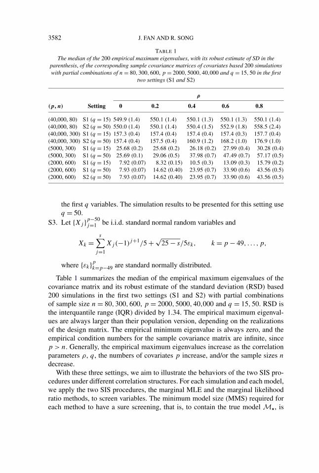
TABLE 1The median of the 200 empirical maximum eigenvalues, with its robust estimate of SD in the
parenthesis, of the corresponding sample covariance matrices of covariates based 200 simulationswith partial combinations of n = 80,300,600, p = 2000,5000,40,000 and q = 15,50 in the first
two settings (S1 and S2)
ρ
(p,n) Setting 0 0.2 0.4 0.6 0.8
(40,000, 80) S1 (q = 15) 549.9 (1.4) 550.1 (1.4) 550.1 (1.3) 550.1 (1.3) 550.1 (1.4)
(40,000, 80) S2 (q = 50) 550.0 (1.4) 550.1 (1.4) 550.4 (1.5) 552.9 (1.8) 558.5 (2.4)
(40,000, 300) S1 (q = 15) 157.3 (0.4) 157.4 (0.4) 157.4 (0.4) 157.4 (0.3) 157.7 (0.4)
(40,000, 300) S2 (q = 50) 157.4 (0.4) 157.5 (0.4) 160.9 (1.2) 168.2 (1.0) 176.9 (1.0)
(5000, 300) S1 (q = 15) 25.68 (0.2) 25.68 (0.2) 26.18 (0.2) 27.99 (0.4) 30.28 (0.4)
(5000, 300) S1 (q = 50) 25.69 (0.1) 29.06 (0.5) 37.98 (0.7) 47.49 (0.7) 57.17 (0.5)
(2000, 600) S1 (q = 15) 7.92 (0.07) 8.32 (0.15) 10.5 (0.3) 13.09 (0.3) 15.79 (0.2)
(2000, 600) S1 (q = 50) 7.93 (0.07) 14.62 (0.40) 23.95 (0.7) 33.90 (0.6) 43.56 (0.5)
(2000, 600) S2 (q = 50) 7.93 (0.07) 14.62 (0.40) 23.95 (0.7) 33.90 (0.6) 43.56 (0.5)
the first q variables. The simulation results to be presented for this setting useq = 50.
S3. Let {Xj }p−50j=1 be i.i.d. standard normal random variables and
Xk =s∑
j=1
Xj(−1)j+1/5 + √25 − s/5εk, k = p − 49, . . . , p,
where {εk}pk=p−49 are standard normally distributed.
Table 1 summarizes the median of the empirical maximum eigenvalues of thecovariance matrix and its robust estimate of the standard deviation (RSD) based200 simulations in the first two settings (S1 and S2) with partial combinationsof sample size n = 80,300,600, p = 2000,5000,40,000 and q = 15,50. RSD isthe interquantile range (IQR) divided by 1.34. The empirical maximum eigenval-ues are always larger than their population version, depending on the realizationsof the design matrix. The empirical minimum eigenvalue is always zero, and theempirical condition numbers for the sample covariance matrix are infinite, sincep > n. Generally, the empirical maximum eigenvalues increase as the correlationparameters ρ, q , the numbers of covariates p increase, and/or the sample sizes n
decrease.With these three settings, we aim to illustrate the behaviors of the two SIS pro-
cedures under different correlation structures. For each simulation and each model,we apply the two SIS procedures, the marginal MLE and the marginal likelihoodratio methods, to screen variables. The minimum model size (MMS) required foreach method to have a sure screening, that is, to contain the true model M�, is
SIS IN GLIM 3583
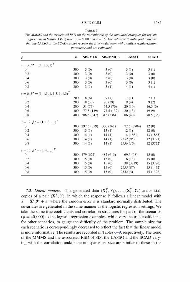
used as a measure of the effectiveness of a screening method. This avoids theissues of choosing the thresholding parameter. To gauge the difficulty of the prob-lem, we also include the LASSO and the SCAD as references for comparisonwhen p = 2000 and 5000. The smaller p is used due to the computation burden ofthe LASSO and the SCAD. In addition, as demonstrated in our simulation results,they do not perform well when p is large. Our initial intension is to demonstratethat the simple SIS does not perform much worse than the far more complicatedprocedures like the LASSO and the SCAD. To our surprise, the SIS can even out-perform those more complicated methods in terms of variable screening. Again,we record the MMS for the LASSO and the SCAD for each simulation and eachmodel, which does not depend on the choice of regularization parameters. Whenthe LASSO or the SCAD cannot recover the true model even with the smallestregularization parameter, we average the model size with the smallest regulariza-tion parameter and p. These interpolated MMS’ are presented with italic font inTables 3–5 and 9 to distinguish from the real MMS. Results for logistic regressionsand linear regressions are presented in the following two subsections.
7.1. Logistic regressions. The generated data (XT1 , Y1), . . . , (XT
n , Yn) are n
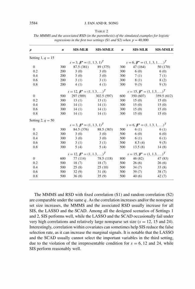
i.i.d. copies of a pair (XT , Y ), in which the conditional distribution of the re-sponse Y given X = x is binomial distribution with probability of success p(x) =exp(xT β�)/[1 + exp(xT β�)]. We vary the size of the nonsparse set of coefficientsas s = 3,6,12,15 and 24. For each simulation, we evaluate each method by sum-marizing the median minimum model size (MMMS) of the selected models as wellas its associated RSD, which is the associated interquartile range (IQR) divided by1.34. The results, based on 200 simulations for each scenario are recorded in thesecond and third panel of Table 2 and the second panel of Tables 3–5. Specifically,Table 2 records the MMMS and the associated RSD for SIS under the first two set-tings when p = 40,000, while Tables 3–5 record these results for SIS, the LASSOand the SCAD when p = 2000 and 5000 under Settings 1, 2 and 3, respectively.The true parameters are also recorded in each corresponding table.
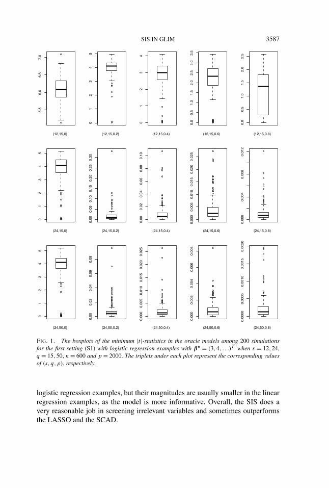
To demonstrate the difficulty of our simulated models, we depict the distribu-tion, among 200 simulations, of the minimum |t |-statistics of s estimated regres-sion coefficients in the oracle model in which the statistician does not know thatall variables are statistically significant. This shows the difficulty in recovering allsignificant variables even in the oracle model with the minimum model size s. Thedistribution was computed for each setting and scenario but only a few selectedsettings are shown presented in Figure 1. In fact, the distributions under Setting 1are very similar to those under Setting 2 when the same q value is taken. It can beseen that the magnitude of the minimum |t |-statistics is reasonably small and get-ting smaller as the correlation within covariates (measured by ρ and q) increases,sometimes achieving three decimals. Given such small signal-to-noise ratio in theoracle models, the difficulty of our simulation models is a self-evident even if thesignals seem not that small.
3584 J. FAN AND R. SONG
TABLE 2The MMMS and the associated RSD (in the parenthesis) of the simulated examples for logistic
regressions in the first two settings (S1 and S2) when p = 40,000
ρ n SIS-MLR SIS-MMLE n SIS-MLR SIS-MMLE
Setting 1, q = 15s = 3, β� = (1,1.3,1)T s = 6, β� = (1,1,3,1, . . .)T
0 300 87.5 (381) 89 (375) 300 47 (164) 50 (170)
0.2 200 3 (0) 3 (0) 300 6 (0) 6 (0)
0.4 200 3 (0) 3 (0) 300 7 (1) 7 (1)
0.6 200 3 (1) 3 (1) 300 8 (1) 8 (2)
0.8 200 4 (1) 4 (1) 300 9 (3) 9 (3)
s = 12, β� = (1,1.3, . . .)T s = 15, β� = (1,1.3, . . .)T
0 500 297 (589) 302.5 (597) 600 350 (607) 359.5 (612)
0.2 300 13 (1) 13 (1) 300 15 (0) 15 (0)
0.4 300 14 (1) 14 (1) 300 15 (0) 15 (0)
0.6 300 14 (1) 14 (1) 300 15 (0) 15 (0)
0.8 300 14 (1) 14 (1) 300 15 (0) 15 (0)
Setting 2, q = 50s = 3, β� = (1,1.3,1)T s = 6, β� = (1,1.3,1, . . .)T
0 300 84.5 (376) 88.5 (383) 500 6 (1) 6 (1)
0.2 300 3 (0) 3 (0) 500 6 (0) 6 (0)
0.4 300 3 (0) 3 (0) 500 6 (1) 6 (1)
0.6 300 3 (1) 3 (1) 500 8.5 (4) 9 (5)
0.8 300 5 (4) 5 (4) 500 13.5 (8) 14 (8)
s = 12, β� = (1,1.3, . . .)T s = 15, β� = (1,1.3, . . .)T
0 600 77 (114) 78.5 (118) 800 46 (82) 47 (83)
0.2 500 18 (7) 18 (7) 500 26 (6) 26 (6)
0.4 500 25 (8) 25 (10) 500 34 (7) 33 (8)
0.6 500 32 (9) 31 (8) 500 39 (7) 38 (7)
0.8 500 36 (8) 35 (9) 500 40 (6) 42 (7)
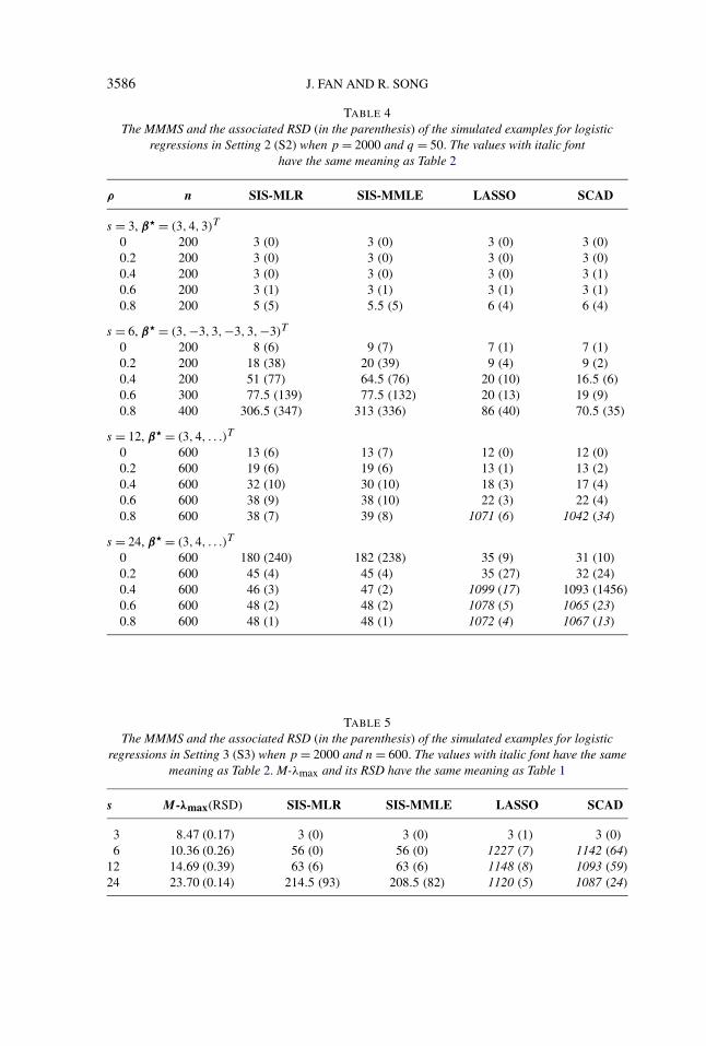
The MMMS and RSD with fixed correlation (S1) and random correlation (S2)are comparable under the same q . As the correlation increases and/or the nonsparseset size increases, the MMMS and the associated RSD usually increase for allSIS, the LASSO and the SCAD. Among all the designed scenarios of Settings 1and 2, SIS performs well, while the LASSO and the SCAD occasionally fail undervery high correlations and relatively large nonsparse set size (s = 12, 15 and 24).Interestingly, correlation within covariates can sometimes help SIS reduce the falseselection rate, as it can increase the marginal signals. It is notable that the LASSOand the SCAD usually cannot select the important variables in the third setting,due to the violation of the irrepresentable condition for s = 6,12 and 24, whileSIS perform reasonably well.
SIS IN GLIM 3585
TABLE 3The MMMS and the associated RSD (in the parenthesis) of the simulated examples for logisticregressions in Setting 1 (S1) when p = 5000 and q = 15. The values with italic font indicatethat the LASSO or the SCAD cannot recover the true model even with smallest regularization
parameter and are estimated
ρ n SIS-MLR SIS-MMLE LASSO SCAD
s = 3, β� = (1,1.3,1)T
0 300 3 (0) 3 (0) 3 (1) 3 (1)
0.2 300 3 (0) 3 (0) 3 (0) 3 (0)
0.4 300 3 (0) 3 (0) 3 (0) 3 (0)
0.6 300 3 (0) 3 (0) 3 (0) 3 (1)
0.8 300 3 (1) 3 (1) 4 (1) 4 (1)
s = 6, β� = (1,1.3,1,1.3,1,1.3)T
0 200 8 (6) 9 (7) 7 (1) 7 (1)
0.2 200 18 (38) 20 (39) 9 (4) 9 (2)
0.4 200 51 (77) 64.5 (76) 20 (10) 16.5 (6)
0.6 300 77.5 (139) 77.5 (132) 20 (13) 19 (9)
0.8 400 306.5 (347) 313 (336) 86 (40) 70.5 (35)
s = 12, β� = (1,1.3, . . .)T
0 300 297.5 (359) 300 (361) 72.5 (3704) 12 (0)
0.2 300 13 (1) 13 (1) 12 (1) 12 (0)
0.4 300 14 (1) 14 (1) 14 (1861) 13 (1865)
0.6 300 14 (1) 14 (1) 2552 (85) 12 (3721)
0.8 300 14 (1) 14 (1) 2556 (10) 12 (3722)
s = 15, β� = (3,4, . . .)T
0 300 479 (622) 482 (615) 69.5 (68) 15 (0)
0.2 300 15 (0) 15 (0) 16 (13) 15 (0)
0.4 300 15 (0) 15 (0) 38 (3719) 15 (3720)
0.6 300 15 (0) 15 (0) 2555 (87) 15 (1472)
0.8 300 15 (0) 15 (0) 2552 (8) 15 (1322)
7.2. Linear models. The generated data (XT1 , Y1), . . . , (XT
n , Yn) are n i.i.d.copies of a pair (XT , Y ), in which the response Y follows a linear model withY = XT β� + ε, where the random error ε is standard normally distributed. Thecovariates are generated in the same manner as the logistic regression settings. Wetake the same true coefficients and correlation structures for part of the scenarios(p = 40,000) as the logistic regression examples, while vary the true coefficientsfor other scenarios, to gauge the difficulty of the problem. The sample size foreach scenario is correspondingly decreased to reflect the fact that the linear modelis more informative. The results are recorded in Tables 6–9, respectively. The trendof the MMMS and the associated RSD of SIS, the LASSO and the SCAD vary-ing with the correlation and/or the nonsparse set size are similar to these in the
3586 J. FAN AND R. SONG
TABLE 4The MMMS and the associated RSD (in the parenthesis) of the simulated examples for logistic
regressions in Setting 2 (S2) when p = 2000 and q = 50. The values with italic fonthave the same meaning as Table 2
ρ n SIS-MLR SIS-MMLE LASSO SCAD
s = 3, β� = (3,4,3)T
0 200 3 (0) 3 (0) 3 (0) 3 (0)
0.2 200 3 (0) 3 (0) 3 (0) 3 (0)
0.4 200 3 (0) 3 (0) 3 (0) 3 (1)
0.6 200 3 (1) 3 (1) 3 (1) 3 (1)
0.8 200 5 (5) 5.5 (5) 6 (4) 6 (4)
s = 6, β� = (3,−3,3,−3,3,−3)T
0 200 8 (6) 9 (7) 7 (1) 7 (1)
0.2 200 18 (38) 20 (39) 9 (4) 9 (2)
0.4 200 51 (77) 64.5 (76) 20 (10) 16.5 (6)
0.6 300 77.5 (139) 77.5 (132) 20 (13) 19 (9)
0.8 400 306.5 (347) 313 (336) 86 (40) 70.5 (35)
s = 12, β� = (3,4, . . .)T
0 600 13 (6) 13 (7) 12 (0) 12 (0)
0.2 600 19 (6) 19 (6) 13 (1) 13 (2)
0.4 600 32 (10) 30 (10) 18 (3) 17 (4)
0.6 600 38 (9) 38 (10) 22 (3) 22 (4)
0.8 600 38 (7) 39 (8) 1071 (6) 1042 (34)
s = 24, β� = (3,4, . . .)T
0 600 180 (240) 182 (238) 35 (9) 31 (10)
0.2 600 45 (4) 45 (4) 35 (27) 32 (24)
0.4 600 46 (3) 47 (2) 1099 (17) 1093 (1456)
0.6 600 48 (2) 48 (2) 1078 (5) 1065 (23)
0.8 600 48 (1) 48 (1) 1072 (4) 1067 (13)
TABLE 5The MMMS and the associated RSD (in the parenthesis) of the simulated examples for logistic
regressions in Setting 3 (S3) when p = 2000 and n = 600. The values with italic font have the samemeaning as Table 2. M-λmax and its RSD have the same meaning as Table 1
s M-λmax(RSD) SIS-MLR SIS-MMLE LASSO SCAD
3 8.47 (0.17) 3 (0) 3 (0) 3 (1) 3 (0)
6 10.36 (0.26) 56 (0) 56 (0) 1227 (7) 1142 (64)
12 14.69 (0.39) 63 (6) 63 (6) 1148 (8) 1093 (59)
24 23.70 (0.14) 214.5 (93) 208.5 (82) 1120 (5) 1087 (24)
SIS IN GLIM 3587
FIG. 1. The boxplots of the minimum |t |-statistics in the oracle models among 200 simulationsfor the first setting (S1) with logistic regression examples with β� = (3,4, . . .)T when s = 12,24,q = 15,50, n = 600 and p = 2000. The triplets under each plot represent the corresponding valuesof (s, q, ρ), respectively.
logistic regression examples, but their magnitudes are usually smaller in the linearregression examples, as the model is more informative. Overall, the SIS does avery reasonable job in screening irrelevant variables and sometimes outperformsthe LASSO and the SCAD.
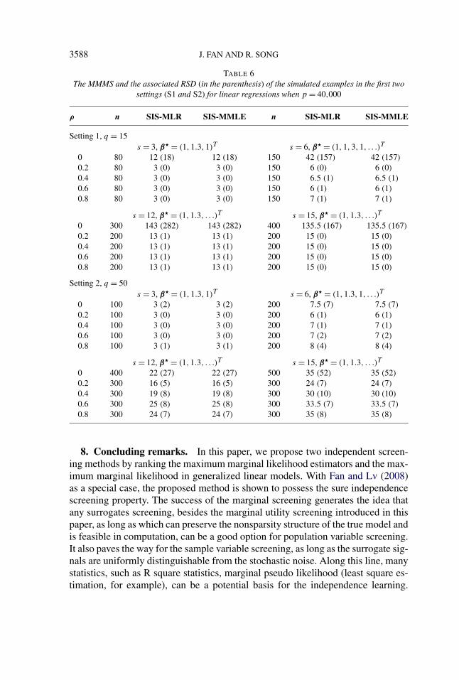
3588 J. FAN AND R. SONG
TABLE 6The MMMS and the associated RSD (in the parenthesis) of the simulated examples in the first two
settings (S1 and S2) for linear regressions when p = 40,000
ρ n SIS-MLR SIS-MMLE n SIS-MLR SIS-MMLE
Setting 1, q = 15s = 3, β� = (1,1.3,1)T s = 6, β� = (1,1,3,1, . . .)T
0 80 12 (18) 12 (18) 150 42 (157) 42 (157)
0.2 80 3 (0) 3 (0) 150 6 (0) 6 (0)
0.4 80 3 (0) 3 (0) 150 6.5 (1) 6.5 (1)
0.6 80 3 (0) 3 (0) 150 6 (1) 6 (1)
0.8 80 3 (0) 3 (0) 150 7 (1) 7 (1)
s = 12, β� = (1,1.3, . . .)T s = 15, β� = (1,1.3, . . .)T
0 300 143 (282) 143 (282) 400 135.5 (167) 135.5 (167)
0.2 200 13 (1) 13 (1) 200 15 (0) 15 (0)
0.4 200 13 (1) 13 (1) 200 15 (0) 15 (0)
0.6 200 13 (1) 13 (1) 200 15 (0) 15 (0)
0.8 200 13 (1) 13 (1) 200 15 (0) 15 (0)
Setting 2, q = 50s = 3, β� = (1,1.3,1)T s = 6, β� = (1,1.3,1, . . .)T
0 100 3 (2) 3 (2) 200 7.5 (7) 7.5 (7)
0.2 100 3 (0) 3 (0) 200 6 (1) 6 (1)
0.4 100 3 (0) 3 (0) 200 7 (1) 7 (1)
0.6 100 3 (0) 3 (0) 200 7 (2) 7 (2)
0.8 100 3 (1) 3 (1) 200 8 (4) 8 (4)
s = 12, β� = (1,1.3, . . .)T s = 15, β� = (1,1.3, . . .)T
0 400 22 (27) 22 (27) 500 35 (52) 35 (52)
0.2 300 16 (5) 16 (5) 300 24 (7) 24 (7)
0.4 300 19 (8) 19 (8) 300 30 (10) 30 (10)
0.6 300 25 (8) 25 (8) 300 33.5 (7) 33.5 (7)
0.8 300 24 (7) 24 (7) 300 35 (8) 35 (8)
8. Concluding remarks. In this paper, we propose two independent screen-ing methods by ranking the maximum marginal likelihood estimators and the max-imum marginal likelihood in generalized linear models. With Fan and Lv (2008)as a special case, the proposed method is shown to possess the sure independencescreening property. The success of the marginal screening generates the idea thatany surrogates screening, besides the marginal utility screening introduced in thispaper, as long as which can preserve the nonsparsity structure of the true model andis feasible in computation, can be a good option for population variable screening.It also paves the way for the sample variable screening, as long as the surrogate sig-nals are uniformly distinguishable from the stochastic noise. Along this line, manystatistics, such as R square statistics, marginal pseudo likelihood (least square es-timation, for example), can be a potential basis for the independence learning.
SIS IN GLIM 3589
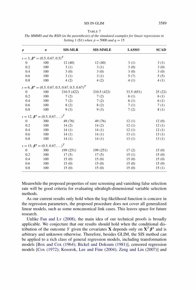
TABLE 7The MMMS and the RSD (in the parenthesis) of the simulated examples for linear regressions in
Setting 1 (S1) when p = 5000 and q = 15
ρ n SIS-MLR SIS-MMLE LASSO SCAD
s = 3, β� = (0.5,0.67,0.5)T
0 100 12 (40) 12 (40) 3 (1) 3 (1)
0.2 100 3 (1) 3 (1) 3 (0) 3 (0)
0.4 100 3 (0) 3 (0) 3 (0) 3 (0)
0.6 100 3 (1) 3 (1) 5 (7) 5 (5)
0.8 100 4 (2) 4 (2) 4 (1) 4 (1)
s = 6, β� = (0.5,0.67,0.5,0.67,0.5,0.67)T
0 100 210.5 (422) 210.5 (422) 33.5 (651) 25 (22)
0.2 100 7 (2) 7 (2) 6 (1) 6 (1)
0.4 100 7 (2) 7 (2) 6 (1) 6 (1)
0.6 100 8 (2) 8 (2) 7 (1) 7 (1)
0.8 100 9 (3) 9 (3) 7 (2) 8 (1)
s = 12, β� = (0.5,0.67, . . .)T
0 300 49 (76) 49 (76) 12 (1) 12 (0)
0.2 100 14 (2) 14 (2) 12 (1) 12 (1)
0.4 100 14 (1) 14 (1) 12 (1) 12 (1)
0.6 100 14 (1) 14 (1) 13 (1) 13 (1)
0.8 100 14 (1) 14 (1) 13 (1) 13 (1)
s = 15, β� = (0.5,0.67, . . .)T
0 300 199 (251) 199 (251) 17 (2) 15 (0)
0.2 100 17 (5) 17 (5) 15 (1) 15 (0)
0.4 100 15 (0) 15 (0) 15 (0) 15 (0)
0.6 100 15 (0) 15 (0) 15 (0) 15 (0)
0.8 100 15 (0) 15 (0) 15 (0) 15 (1)
Meanwhile the proposed properties of sure screening and vanishing false selectionrate will be good criteria for evaluating ultrahigh-dimensional variable selectionmethods.
As our current results only hold when the log-likelihood function is concave inthe regression parameters, the proposed procedure does not cover all generalizedlinear models, such as some noncanonical link cases. This leaves space for futureresearch.
Unlike Fan and Lv (2008), the main idea of our technical proofs is broadlyapplicable. We conjecture that our results should hold when the conditional dis-tribution of the outcome Y given the covariates X depends only on XT β� and isarbitrary and unknown otherwise. Therefore, besides GLIM, the SIS method canbe applied to a rich class of general regression models, including transformationmodels [Box and Cox (1964); Bickel and Doksum (1981)], censored regressionmodels [Cox (1972); Kosorok, Lee and Fine (2004); Zeng and Lin (2007)] and
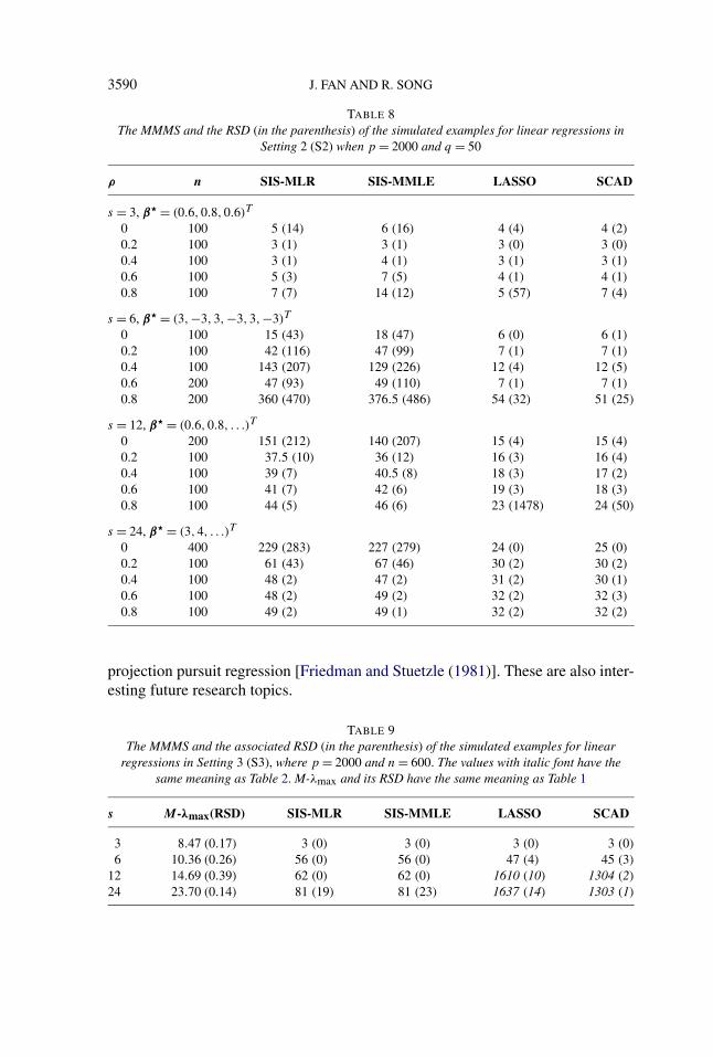
3590 J. FAN AND R. SONG
TABLE 8The MMMS and the RSD (in the parenthesis) of the simulated examples for linear regressions in
Setting 2 (S2) when p = 2000 and q = 50
ρ n SIS-MLR SIS-MMLE LASSO SCAD
s = 3, β� = (0.6,0.8,0.6)T
0 100 5 (14) 6 (16) 4 (4) 4 (2)
0.2 100 3 (1) 3 (1) 3 (0) 3 (0)
0.4 100 3 (1) 4 (1) 3 (1) 3 (1)
0.6 100 5 (3) 7 (5) 4 (1) 4 (1)
0.8 100 7 (7) 14 (12) 5 (57) 7 (4)
s = 6, β� = (3,−3,3,−3,3,−3)T
0 100 15 (43) 18 (47) 6 (0) 6 (1)
0.2 100 42 (116) 47 (99) 7 (1) 7 (1)
0.4 100 143 (207) 129 (226) 12 (4) 12 (5)
0.6 200 47 (93) 49 (110) 7 (1) 7 (1)
0.8 200 360 (470) 376.5 (486) 54 (32) 51 (25)
s = 12, β� = (0.6,0.8, . . .)T
0 200 151 (212) 140 (207) 15 (4) 15 (4)
0.2 100 37.5 (10) 36 (12) 16 (3) 16 (4)
0.4 100 39 (7) 40.5 (8) 18 (3) 17 (2)
0.6 100 41 (7) 42 (6) 19 (3) 18 (3)
0.8 100 44 (5) 46 (6) 23 (1478) 24 (50)
s = 24, β� = (3,4, . . .)T
0 400 229 (283) 227 (279) 24 (0) 25 (0)
0.2 100 61 (43) 67 (46) 30 (2) 30 (2)
0.4 100 48 (2) 47 (2) 31 (2) 30 (1)
0.6 100 48 (2) 49 (2) 32 (2) 32 (3)
0.8 100 49 (2) 49 (1) 32 (2) 32 (2)
projection pursuit regression [Friedman and Stuetzle (1981)]. These are also inter-esting future research topics.
TABLE 9The MMMS and the associated RSD (in the parenthesis) of the simulated examples for linear
regressions in Setting 3 (S3), where p = 2000 and n = 600. The values with italic font have thesame meaning as Table 2. M-λmax and its RSD have the same meaning as Table 1
s M-λmax(RSD) SIS-MLR SIS-MMLE LASSO SCAD
3 8.47 (0.17) 3 (0) 3 (0) 3 (0) 3 (0)
6 10.36 (0.26) 56 (0) 56 (0) 47 (4) 45 (3)
12 14.69 (0.39) 62 (0) 62 (0) 1610 (10) 1304 (2)
24 23.70 (0.14) 81 (19) 81 (23) 1637 (14) 1303 (1)
SIS IN GLIM 3591
Another important extension is to generalize the concept of marginal regressionto the marginal group regression, where the number of covariates m in each mar-ginal regression is greater or equal to one. This leads to a new procedure calledgrouped variables screening. It is expected to improve the situation when the vari-ables are highly correlated and jointly important, but marginally the correlationbetween each individual variable and the response is weak. The current theoreti-cal studies for the componentwise marginal regression can be directly extended togroup variable screening, with appropriate conditions and adjustments. This leadsto another interesting topic of future research.
In practice, how to choose the tuning parameter γn is an interesting and impor-tant problem. As discussed in Fan and Lv (2008), for the first stage of the iterativeSIS procedure, our preference is to select sufficiently many features, such that|Mγn | = n or n/ log(n). The FDR-based methods in multiple comparison can alsopossibly employed. In the second or final stage, Bayes information type of crite-rion can be applied. In practice, some data-driven methods may also be welcomefor choosing the tuning parameter γn. This is an interesting future research topicand is beyond the scope of the current paper.
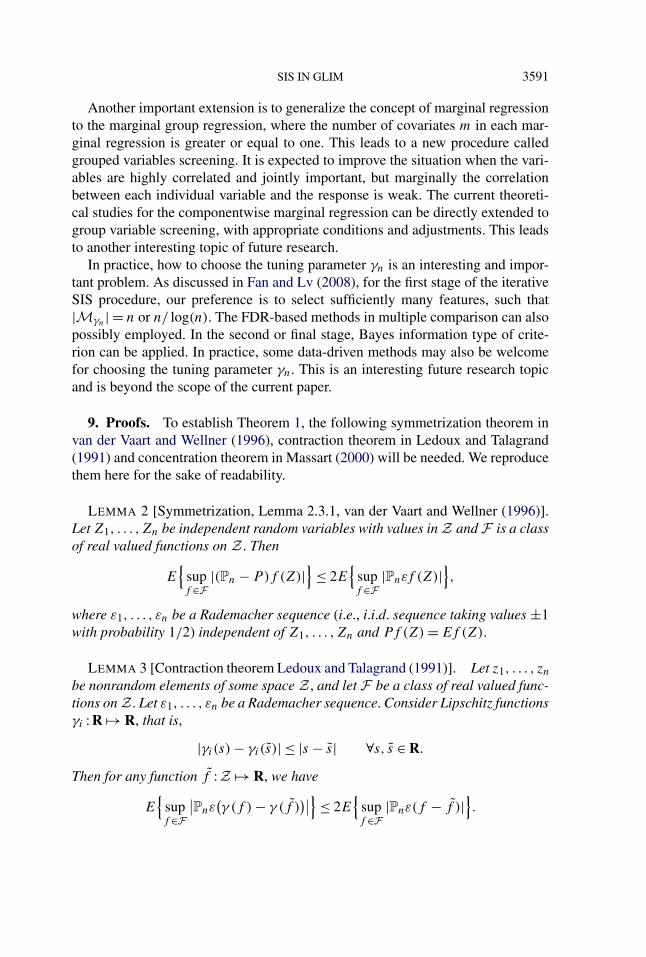
9. Proofs. To establish Theorem 1, the following symmetrization theorem invan der Vaart and Wellner (1996), contraction theorem in Ledoux and Talagrand(1991) and concentration theorem in Massart (2000) will be needed. We reproducethem here for the sake of readability.
LEMMA 2 [Symmetrization, Lemma 2.3.1, van der Vaart and Wellner (1996)].Let Z1, . . . ,Zn be independent random variables with values in Z and F is a classof real valued functions on Z . Then
E{
supf ∈F
|(Pn − P)f (Z)|}
≤ 2E{
supf ∈F
|Pnεf (Z)|},
where ε1, . . . , εn be a Rademacher sequence (i.e., i.i.d. sequence taking values ±1with probability 1/2) independent of Z1, . . . ,Zn and Pf (Z) = Ef (Z).
LEMMA 3 [Contraction theorem Ledoux and Talagrand (1991)]. Let z1, . . . , zn
be nonrandom elements of some space Z , and let F be a class of real valued func-tions on Z . Let ε1, . . . , εn be a Rademacher sequence. Consider Lipschitz functionsγi : R �→ R, that is,
|γi(s) − γi(s)| ≤ |s − s| ∀s, s ∈ R.
Then for any function f : Z �→ R, we have
E{
supf ∈F
∣∣Pnε(γ (f ) − γ (f )
)∣∣} ≤ 2E{
supf ∈F
|Pnε(f − f )|}.
3592 J. FAN AND R. SONG
LEMMA 4 [Concentration theorem Massart (2000)]. Let Z1, . . . ,Zn be inde-pendent random variables with values in some space Z and let γ ∈ �, a class ofreal valued functions on Z . We assume that for some positive constants li,γ andui,γ , li,γ ≤ γ (Zi) ≤ ui,γ ∀γ ∈ �. Define
L2 = supγ∈�
n∑i=1
(ui,γ − li,γ )2/n
and
Z = supγ∈�
|(Pn − P)γ (Z)|,
then for any t > 0,
P(Z ≥ EZ + t) ≤ exp(− nt2
2L2
).
Let N > 0, define a set of β
B(N) = {β ∈ B,‖β − β0‖ ≤ N}.Let
G1(N) = supβ∈B(N)
|(Pn − P){l(XT β, Y ) − l(XT β0, Y )}In(X, Y )|,
where In(X, Y ) is defined in condition B. The next result is about the upper boundof the tail probability for G1(N) in the neighborhood of B(N).
LEMMA 5. For all t > 0, it holds that
P(G1(N) ≥ 4Nkn(q/n)1/2(1 + t)
) ≤ exp(−2t2/K2n).
PROOF. The main idea is to apply the concentration theorem (Lemma 4). Tothis end, we first show that the random variables involved are bounded. By condi-tion B and the Cauchy–Schwarz inequality, we have that on the set �n,
|l(XT β, Y ) − l(XT β0, Y )| ≤ kn|XT (β − β0)| ≤ kn‖X‖‖β − β0‖.On the set �n, by the definition of B(N), the above random variable is furtherbounded by knq
1/2KnN . Hence, L2 = 4k2nqK2
nN2, using the notation of Lemma 4.We need to bound the expectation EG1(N). An application of the symmetriza-
tion theorem (Lemma 2) yields that
EG1(N) ≤ 2E[
supβ∈B(N)
|Pnε{l(XT β, Y ) − l(XT β0, Y )}In(X, Y )|].
SIS IN GLIM 3593
By the contraction theorem (Lemma 3), and the Lipschitz condition in condition B,we can bound the right-hand side of the above inequality further by
4knE{
supβ∈B(N)
|PnεXT (β − β0)In(X, Y )|}.(6)
By the Cauchy–Schwarz inequality, the expectation in (6) is controlled by
E‖PnεXIn(X, Y )‖ supβ∈B(N)
‖β − β0‖ ≤ E‖PnεXIn(X, Y )‖N.(7)
By Jensen’s inequality, the expectation in (7) is bounded above by
(E‖PnεXIn(X, Y )‖2)1/2 = (E‖X‖2In(X, Y )/n
)1/2 ≤ (q/n)1/2,
by noticing that
E‖X‖2In(X, Y ) ≤ E‖X‖2 = E(X21 + · · · + X2
q) = q,
since EX2j = 1. Combining these results, we conclude that
EG1(N) ≤ 4Nkn(q/n)1/2.
An application of the concentration theorem (Lemma 4) yields that
P(G1(N) ≥ 4Nkn(q/n)1/2(1 + t)
) ≤ exp(−n{4Nkn(q/n)1/2t}2
8qK2nk2
nN2
)= exp(−2t2/K2
n).
This proves the lemma. �
PROOF OF THEOREM 1. The proof takes two main steps: we first bound ‖β −β0‖ by G(N) for a small N , where N chosen so that conditions B and C hold, andthen utilize Lemma 5 to conclude.
Following a similar idea in van de Geer (2002), we define a convex combinationβs = sβ + (1 − s)β0 with
s = (1 + ‖β − β0‖/N)−1.
Then, by definition,
‖βs − β0‖ = s‖β − β0‖ ≤ N,
namely, βs ∈ B(N). Due to the convexity, we have
Pnl(XT βs, Y ) ≤ sPnl(XT β, Y ) + (1 − s)Pnl(XT β0, Y )(8)
≤ Pnl(XT β0, Y ).
Since β0 is the minimizer, we have
E[l(XT βs, Y ) − l(XT β0, Y )] ≥ 0,
3594 J. FAN AND R. SONG
where βs is regarded a parameter in the above expectation. Hence, it follows from(8) that
E[l(XT βs, Y ) − l(XT β0, Y )]≤ (E − Pn)[l(XT βs, Y ) − l(XT β0, Y )]≤ G(N),
where
G(N) = supβ∈B(N)
|(Pn − P){l(XT β, Y ) − l(XT β0, Y )}|.
By condition C, it follows that
‖βs − β0‖ ≤ [G(N)/Vn]1/2.(9)
We now use (9) to conclude the result. Note that for any x,
P(‖βs − β0‖ ≥ x) ≤ P(G(N) ≥ Vnx
2).
Setting x = N/2, we have
P(‖βs − β0‖ ≥ N/2) ≤ P {G(N) ≥ VnN2/4}.
Using the definition of βs , the left-hand side is the same as P {‖β − β0‖ ≥ N}.Now, by taking N = 4an(1 + t)/Vn with an = 4kn
√q/n, we have
P {‖β − β0‖ ≥ N} ≤ P {G(N) ≥ VnN2/4}
= P {G(N) ≥ Nan(1 + t)}.The last probability is bounded by
P {G(N) ≥ Nan(1 + t),�n,�} + P {�cn,�},(10)
where �n,� = {‖Xi‖ ≤ Kn, |Yi | ≤ K�n}.
On the set �n,�, since
supβ∈B(N)
Pn|l(XT β, Y ) − l(XT β0, Y )|(1 − In(X, Y )) = 0,
by the triangular inequality,
G(N) ≤ G1(N) + supβ∈B(N)
∣∣E[l(XT β, Y ) − l(XT β0, Y )](1 − In(X, Y ))∣∣.
It follows from condition B that (10) is bounded by
P {G1(N) ≥ Nan(1 + t) + o(q/n)} + nP {(X, Y ) ∈ �cn}.
The conclusion follows from Lemma 5. �

SIS IN GLIM 3595
PROOF OF THEOREM 2. First of all, the target function El(β0 + βjXj ,Y ) isa convex function in βj . We first show that if cov(b′(XT β�),Xj ) = 0, then βM
j
must be zero. Recall EXj = 0. The score equation of the marginal regression atβM
j takes the form
E{b′(XTj βM
j )Xj } = E(YXj ) = E{b′(XT β�)Xj }.It can be equivalently written as
cov(b′(XTj βM
j ),Xj ) = cov(b′(XT β�),Xj ) = 0.
Since both functions f (t) = b′(βMj,0 + t) and h(t) = t are strictly monotone in t ,
when t �= 0,
{f (t) − f (0)}(t − 0) > 0.
If βMj �= 0, let t = βM
j Xj ,
βMj cov(f (βM
j Xj ),Xj ) = E[E{f (t) − f (0)}(t − 0)|Xj �= 0] > 0,
which leads to a contradiction. Hence βMj must be zero.
On the other side, if βMj = 0, the score equations now take the form
E{b′(βMj,0)} = E{b′(XT β�)}(11)
and
E{b′(βMj,0)Xj } = E{b′(XT β�)Xj }.(12)
Since b′(βMj,0) is a constant, we can get the desired result by plugging (11) into (12).
�
PROOF OF THEOREM 3. We first prove the case that b′′(θ) is bounded. By theLipschitz continuity of the function b′(·), we have
|{b′(βMj,0 + Xjβ
Mj ) − b′(βM
j,0)}Xj | ≤ D1|βMj |X2
j .
D1 = supx b′′(x). By taking the expectation on both sides, we have
|E{b′(βMj,0 + Xjβ
Mj ) − b′(βM
j,0)}Xj | ≤ D1|βMj |,
namely,
D1|βMj | ≥ | cov(b′(βM
j,0 + XjβMj ),Xj )|.(13)
Note that βMj,0 and βM
j satisfy the score equation
E{b′(βM0,1 + βM
j Xj ) − b′(XT β�)}Xj = 0.(14)
3596 J. FAN AND R. SONG
It follows from (13) and EXj = 0 that
|βMj | ≥ D−1
1 c1n−κ .
The conclusion follows.We now prove the second case. The result holds trivially if |βM
j | ≥ cn−κ for a
sufficiently large universal constant c. Now suppose that |βMj | ≤ c9n
−κ , for some
positive constant c9. We will show later that |βMj,0 − βM
0 | ≤ c10 for some c10 > 0,
where βM0 is such that b′(βM
0 ) = EY . In this case, if |Xj | ≤ nκ , then the pointsβM
j,0 and (βMj,0 + Xjβ
Mj ) falls in the interval βM
0 ± h, independent of j , whereh = c9 + c10.
By the Lipschitz continuity of the function b′(·) in the neighborhood aroundβM
0 , we have for |Xj | ≤ nκ ,
|{b′(βMj,0 + Xjβ
Mj ) − b′(βM
j,0)}Xj | ≤ D2|βMj |X2
j ,
where D2 = maxx∈[βM0 −h,βM
0 +h] b′′(x). By taking the expectation on both sides, itfollows that
|E{b′(βMj,0 + Xjβ
Mj ) − b′(βM
j,0)}XjI (|Xj | ≤ nκ)| ≤ D2|βMj |.(15)
By using (14) and EXj = 0, we deduce from (15) that
D2|βMj | ≥ | cov(XT β�,Xj )| − A0 − A1,(16)
where Am = E|b′(βMj,0 + Xm
j βMj )Xj |I (|Xj | ≥ nκ) for m = 0 and 1. Since |βM
j,0 +Xjβ
Mj | ≤ a|Xj | for |Xj | ≥ nκ for a sufficiently large n, independent of j , by the
condition given in the theorem, we have
Am ≤ EG(a|Xj |)m|Xj |I (|Xj | ≥ nκ) ≤ dn−κ for m = 0 and 1.
The conclusion now follows from (16).It remains to show that when |βM
j | ≤ c9n−κ we have |βM
j,0 − βM0 | ≤ c10. To this
end, let
�(β0) = E{b(β0 + βMj Xj ) − Y(β0 + βM
j Xj )}.Then, it is easy to see that
�′(β0) = Eb′(β0 + βMj Xj ) − b′(βM
0 ).
Observe that
|Eb′(β0 + βMj Xj ) − b′(β0)| ≤ R1 + R2,(17)
where R1 = sup|x|≤c9nη−κ |b′(β0 + x) − b′(β0)| and R2 = 2EG(a|Xj |)I (|Xj | >
nη). Now, R1 = o(1) due to the continuity of b′(·) and R2 = o(1) by the conditionof the theorem. Consequently, by (17), we conclude that
�′(β0) = b′(β0) − b′(βM0 ) + o(1).
SIS IN GLIM 3597
Since b′(·) is a strictly increasing function, it is now obvious that
�′(βM0 − c10) < 0, �′(βM
0 + c10) > 0
for any given c10 > 0. Hence, |βMj,0 − βM
0 | < c10. �
PROOF OF PROPOSITION 1. Without loss of generality, assume that g(·) isstrictly increasing and ρ > 0. Since X and Z are jointly normally distributed, Z
can be expressed as
Z = ρX + ε,
where ρ = E(XZ) is the regression coefficient, and X and ε are independent.Thus,
Ef (Z)X = Eg(ρX)X = E[g(ρX) − g(0)]X,(18)
where g(x) = Ef (x + ε) is a strictly increasing function. The right-hand side of(18) is always nonnegative and is zero if and only if ρ = 0.
To prove the second part, we first note that the random variable on the right-handside of (18) is nonnegative. Thus, by the mean-value theorem, we have that
|Ef (Z)X| ≥ inf|x|≤cρ|g′(x)|ρEX2I (|X| ≤ c).
Hence, the result follows. �
PROOF OF LEMMA 1. By Chebyshev’s inequality,
P(Y ≥ u) ≤ exp(−s0u)E exp(s0Y).
Let θ = XT β�. Since Y belongs to an exponential family, we have
E{exp(s0Y)|θ} = exp(b(θ + s0) − b(θ)
).
Hence
P(Y ≥ u) ≤ exp(−s0u)E exp(b(XT β� + s0) − b(XT β�)
).
Similarly we can get
P(Y ≤ −u) ≤ exp(−s0u)E exp(b(XT β� − s0) − b(XT β�)
).
The desired result thus follows from condition D by letting u = m0tα/s0. �
PROOF OF THEOREM 4. Note that condition B is satisfied with kn defined inSection 5.2. The tail part of condition B can also be easily checked. In fact,
E[l(XTj βj , Y ) − l(βM
j ,Y )](1 − In(Xj , Y ))
≤ ∣∣Eb(XTj βj )I (|Xj | ≥ Kn)
∣∣ + ∣∣Eb(XTj βM
j )I (|Xj | ≥ Kn)∣∣
+ B(βj ) + B(βMj ),

3598 J. FAN AND R. SONG
where B(βj ) = |EYXTj βj (1−In(Xj , Y ))|. The first two terms are of order o(1/n)
by assumption, and the last two terms can be bounded by the exponential tail con-ditions in condition D and the Cauchy–Schwarz inequality.
By Theorem 1, we have for any t > 0,
P(√
n|βMj − βM
j | ≥ 16(1 + t)kn/V) ≤ exp(−2t2/K2
n) + nm1 exp(−m0Kαn ).
By taking 1 + t = c3V n1/2−κ/(16kn), it follows that
P(|βMj − βM
j | ≥ c3n−κ) ≤ exp
(−c4n1−2κ/(knKn)
2) + nm1 exp(−m0Kαn ).
The first result follows from the union bound of probability.To prove the second part, note that on the event
An ≡{
maxj∈M�
|βMj − βM
j | ≤ c2n−κ/2
},
by Theorem 3, we have
|βMj | ≥ c2n
−κ/2 for all j ∈ M�.(19)
Hence, by the choice of γn, we have M� ⊂ Mγn . The result now follows from asimple union bound
P(Acn) ≤ sn
{exp
(−c4n1−2κ/(knKn)
2) + nm1 exp(−m0Kαn )
}.
This completes the proof. �
PROOF OF THEOREM 5. The key idea of the proof is to show that
‖βM‖2 = O(‖�β�‖2) = O{λmax(�)}.(20)
If so, the number of {j : |βMj | > εn−κ} cannot exceed O{n2κλmax(�)} for any ε >
0. Thus, on the set
Bn ={
max1≤j≤pn
|βMj − βM
j | ≤ εn−κ},
the number of {j : |βMj | > 2εn−κ} cannot exceed the number of {j : |βM
j | > εn−κ},which is bounded by O{n2κλmax(�)}. By taking ε = c5/2, we have
P [|Mγn | ≤ O{n2κλmax(�)}] ≥ P(Bn).
The conclusion follows from Theorem 4(i).It remains to prove (20). We first bound βM
j . Since b′(·) is monotonically in-creasing, the function
{b′(βMj,0 + Xjβ
Mj ) − b′(βM
j,0)}XjβMj
is always positive. By Taylor’s expansion, we have
{b′(βMj,0 + Xjβ
Mj ) − b′(βM
j,0)}βMj Xj ≥ D3(β
Mj Xj )
2I (|Xj | ≤ K),
SIS IN GLIM 3599
where D3 = inf|x|≤K(B+1) b′′(x), since (βM
j,0, βMj ) is an interior point of the square
B with length 2B . By taking the expectation on both sides and using EXj = 0, wehave
Eb′(βMj,0 + Xjβ
Mj )βM
j Xj ≥ D3E(βMj Xj )
2I (|Xj | ≤ K).
Since EX2j I (|Xj | ≤ K) = 1 − EX2
j I (|Xj | > K), it is uniformly bounded frombelow for a sufficiently large K , due to the uniform exponential tail bound in con-dition D. Thus, it follows from (12) that
|βMj |2 ≤ D4|Eb′(XT β�)Xj |(21)
for some D4 > 0.We now further bound from above the right-hand side of (21) by using
var(XT β�) = O(1). We first show the case where b′′(·) is bounded. By the Lip-schitz continuity of the function b′(·), we have
|{b′(XT β�) − b′(β�0)}Xj | ≤ D5|Xj XT
Mβ�1|,
where XM = (X1, . . . ,Xpn)T and β�
1 = (β�1, . . . , β�
pn)T .
By putting the above equation into the vector form and taking the expectationon both sides, we have
‖E{b′(XT β�) − b′(β�0)}XM‖2 ≤ D2
5‖EXMXTMβ�
1‖2
(22)≤ D2
5λmax(�)‖�1/2β�‖2.
Using EXM = 0 and var(XT β�) = O(1), we conclude that
‖Eb′(XT β�)XM‖2 ≤ D6λmax(�)
for some positive constant D6. This together with (21) entails (20).It remains to bound (21) for the second case. Since XM = R�
1/21 U, it follows
that
Eb′(β�0 + XT
Mβ�1)XM = Eb′(β�
0 + βT2 RU)R�
1/21 U,
where β2 = �1/21 β�
1. By conditioning on βT2 U, it can be computed that
E(U|βT2 U) = βT
2 U/‖β2‖2β2.
Therefore,
Eb′(β�0 + XT
Mβ�1)XM = Eb′(β�
0 + βT2 RU)R�
1/21 βT
2 U/‖β2‖2β2
= Eb′(XT β�)(XT β� − β�0)�
1/21 β2/‖β2‖2.
This entails that
‖Eb′(XT β�)XM‖2 = |Eb′(XT β�)(XT β� − β0)|2‖�1/21 β2‖2/‖β2‖4.(23)

3600 J. FAN AND R. SONG
By condition G, |Eb′(XT β�)(XT β� −β�0)| = O(1). We also observe the facts that
‖�1/21 β2‖ ≤ λ
1/2max(�)‖β2‖ and that ‖β2‖ = ‖�1/2β�‖ is bounded. This proves
(20) for the second case by using (21) and completes the proof. �
PROOF OF THEOREM 6. If cov(b′(XT β�),Xj ) = 0, by Theorem 2, we haveβM
j = 0, hence by the model identifiability at βM0 , βM
j,0 = βM0 . Hence, L�
j = 0.
On the other hand, if L�j = 0, by condition C′, it follows that βM
j = βM0 , that is,
βMj,0 = βM
0 and βMj = 0. Hence by Theorem 2, cov(b′(XT β�),Xj ) = 0. �
PROOF OF THEOREM 7. If | cov(b′(XT β�),Xj )| ≥ c1n−κ , for j ∈ M�, by
Theorem 3, we have minj∈M� |βMj | ≥ c2n
−κ . The first result thus follows fromcondition C′.
To prove the second result, we will bound L�j . We first show the case where
b′′(·) is bounded. By definition, we have
0 ≤ L�j ≤ E{l(βM
j,0, Y ) − l(XTj βM
j ,Y )}.(24)
By Taylor’s expansion of the right-hand side of (24), we have that
E{l(βMj,0, Y ) − l(XT
j βMj ,Y )} ≤ D5(β
Mj )2 for some D5 > 0.(25)
The desired result thus follows from (24), (25) and the proof in Theorem 5 that
‖L�‖ ≤ O(‖βM‖2) = O(λmax(�)).
Now we prove the second case. By the mean-value theorem,
E{l(βMj,0, Y ) − l(XT
j βMj ,Y )} = E{Y − b′(βM
j,0 + sXjβMj )}Xjβ
Mj(26)
for some 0 < s < 1. Since EYXj = Eb′(XTj βM
j )Xj , the last term is equal to
E{b′(XTj βM
j ) − b′(βMj,0 + sXjβ
Mj )}Xjβ
Mj .(27)
By the monotonicity of b′(·), when XjβMj ≥ 0, both factors in (27) is nonnegative,
and hence
{b′(XTj βM
j )−b′(βMj,0 + sXjβ
Mj )}Xjβ
Mj ≤ {b′(XT
j βMj )−b′(βM
j,0)}XjβMj .(28)
When XjβMj < 0, both factors in (28) are negative and (28) continues to hold. It
follows from (26)–(28) and EXj = 0, the right-hand side of (26) is bounded by
Eb′(XTj βM
j )XjβMj = Eb′(XT β�)Xjβ
Mj .(29)
Combining (24), (26) and (29), we can bound ‖L�‖ in the vector form by theCauchy–Schwarz inequality
‖L�‖ ≤ ‖Eb′(XT β�)XM‖‖βM‖ = O(‖�β�‖‖βM‖),
SIS IN GLIM 3601
where (23) is used in the last equality. The desired result thus follows from Theo-rem 5. �
PROOF OF THEOREM 8. To prove the result, we first bound Lj,n from be-low to show the strength of the signals. Let βM
0 = (βM0 ,0)T . Then, by Taylor’s
expansion, we have
2Lj,n = (βM0 − βM
j )�′′j (ξn)(β
M0 − βM
j ) ≥ λj,min(βMj )2,(30)
where λj,min is the minimum eigenvalue of the Hessian matrix
�′′j (ξn) = Pnb
′′(ξTn Xj )Xj XT
j ,
where ξn lies between βM0 and βM
j . We will show
P {λj,min > c11} = 1 − O{exp(−c12n1−κ)}(31)
for some c11 > 0 and c12 > 0.Suppose (31) holds. Then, by (19), we have
P{
minj∈M�
|βMj | ≥ c2n
−κ/2}
= 1 − O(sn
{exp
(−c4n1−2κ/(knKn)
2) + nm1 exp(−m0Kαn )
}).
This, together with (30) and (31), implies
P{
minj∈M�
Lj,n ≥ c11c22n
−2κ/8}
= 1 − O(sn
{exp
(−c4n1−2κ/(knKn)
2) + nm1 exp(−m0Kαn )
}).
Hence, by choosing the thresholding νn = c7n−2κ , for c7 < c11c
22/8, M� ⊂ Nνn
with the probability tending to one exponentially fast, and the result follows.We now prove (31). It is obvious that
�′′j (ξn) ≥ min|x|≤(B+1)K
b′′(x)PnXj XTj I (|Xj | ≤ K)
for any given K . Since the random variable involved is uniformly bounded in j , itfollows from the Hoeffding inequality [Hoeffding (1963)] that
P{∣∣(Pn − P)Xk
j I (|Xj | ≤ K)∣∣ > ε
} ≤ exp(−2nε2/(4K2k)
)(32)
for any k ≥ 0 and ε > 0. By taking ε = n−κ/2, we have
P{∣∣(Pn − P)Xk
j I (|Xj | ≤ K)∣∣ > n−κ/2} ≤ exp
(−2n1−κ/(4K2k)).
Consequently, with probability tending to one exponentially fast, we have
�′′j (ξn) ≥ min|x|≤(B+1)K
b′′(x)EXj XTj I (|Xj | ≤ K)/2.(33)
3602 J. FAN AND R. SONG
The minimum eigenvalue of the matrix EXj XTj I (|Xj | ≤ K) is
min|a|≤1E
(a2 + 2a
√1 − a2Xj + (1 − a2)X2
j
)I (|Xj | ≤ K).
It is bounded from below by
min|a|≤1E{a2 + (1 − a2)X2
j I (|Xj | ≤ K)} − 2∣∣EXjI (|Xj | ≤ K)
∣∣ − K−2,(34)
where we used P(|Xj | ≥ K) ≤ K−2. Since EXj = 0 and EX2j = 1,∣∣EXjI (|Xj | ≤ K)
∣∣ = ∣∣EXjI (|Xj | > K)∣∣ ≤ K−1EX2
j I (|Xj | > K) ≤ K−1.
Hence the quantity in (34) can be further bounded from below by
EX2j I (|Xj | ≤ K) + min|a|≤1
a2EX2j I (|Xj | > K) − 2K−1 − K−2
≥ 1 − supj
EX2j I (|Xj | > K) − 2K−1 − K−2.
The result follows from condition G and (33). �
PROOF OF THEOREM 9. By (30), it can be easily seen that
2Lj,n ≤ D1λmax(PnXj XTj )‖βM
0 − βMj ‖2,
where D1 = supx b′′(x) as defined in the proof of Theorem 3. By (32), with theexception on a set with negligible probability, it follows that
λmax(PnXj XTj ) ≤ 2λmax(EXj XT
j ) = 2,
uniformly in j . Therefore, with probability tending to one exponentially fast, wehave
Lj,n ≤ D7{(βM0 − βM
j,0)2 + (βM
j )2}(35)
for some D7 > 0.We now use (35) to show that if Lj,n > c7n
−2κ , then |βMj | ≥ D8n
−κ , with ex-
ception on a set with negligible probability, where D8 = {c8/(2D7)}1/2. This im-plies that
|Nνn | ≤ |Mγn |,with γn = D8n
−κ . The conclusion then follows from Theorem 5.We now show that Lj,n > c7n
−2κ implies that |βMj | ≥ D8n
−κ , with exception
on a set with negligible probability. Suppose that |βMj | < D8n
−κ . From the likeli-hood equations, we have
b′(βM0 ) = Y = Pnb
′(βMj,0 + βM
j Xj ).(36)
SIS IN GLIM 3603
From the proof of Theorem 4, with exception on a set with negligible probability,we have |βM
0 − βM0 | ≤ c13n
−κ and |βMj,0 − βM
j,0| ≤ c14n−κ , for some constants
c13 and c14. Since (βM0 ,0) and (βM
j,0, βMj ) are interior points of the square B
with length 2B , it follows that with exception on a set with negligible probabil-ity, |βM
0 | ≤ B and |βMj,0| ≤ B . Recall D1 = supx b′′(x). By Taylor’s expansion, for
some 0 < s < 1, we have
|Pnb′(βM
j,0 + βMj Xj ) − b′(βM
j,0)| = |b′′(βMj,0 + sβM
j Xj )βMj PnXj |
(37)≤ D1|βM
j PnXj | = oP (|βMj |),
where the last step follows from the facts that EXj = 0 and consequently PnXj =o(1) with an exception on a set of negligible probability, by applying the Hoeffdinginequality on �c
n and considering the exponential tail property of Xj . Hence, by(36) and (37), we have
|b′(βM0 ) − b′(βM
j,0)| = oP (|βMj |).
Let D9 = inf|x|≤2B b′′(x), with exception on a set with negligible probability, wehave
|b′(βM0 ) − b′(βM
j,0)| ≥ D9|βM0 − βM
j,0|.Therefore, we conclude that
|βM0 − βM
j,0| = oP (|βMj |).
By (35), we have |βMj | > D8n
−κ . This is a contraction, except on a set that hasa negligible probability. This completes the proof. �
Acknowledgments. The bulk of the work was conducted when Rui Song wasa postdoctoral research fellow at Princeton University. The authors would like tothank the associate editor and two referees for their constructive comments thatimprove the presentation and the results of the paper.
REFERENCES
BICKEL, P. J. and DOKSUM, K. A. (1981). An analysis of transformations revisited. J. Amer. Statist.Assoc. 76 296–311. MR0624332
BICKEL, P. J. and DOKSUM, K. A. (2001). Mathematical Statistics: Basic Ideas and Selected Top-ics, 2nd ed. Prentice Hall, Upper Saddle River, NJ.
BOX, G. E. P. and COX, D. R. (1964). An analysis of transformations. J. R. Stat. Soc. Ser. B 26211–246. MR0192611
CANDES, E. and TAO, T. (2007). The dantzig selector: Statistical estimation when p is much largerthan n (with discussion). Ann. Statist. 35 2313–2404. MR2382644
COX, D. R. (1972). Regression models and life-tables (with discussion). J. R. Stat. Soc. Ser. B Stat.Methodol. 34 187–220. MR0341758
FAHRMEIR, L. and KAUFMANN, H. (1985). Consistency and asymptotic normality of the maximumlikelihood estimator in generalized linear models. Ann. Statist. 13 342–368. MR0773172
3604 J. FAN AND R. SONG
FAN, J. and FAN, Y. (2008). High-dimensional classification using features annealed independencerules. Ann. Statist. 36 2605–2637. MR2485009
FAN, J. and LI, R. (2001). Variable selection via nonconcave penalized likelihood and its oracleproperties. J. Amer. Statist. Assoc. 96 1348–1360. MR1946581
FAN, J. and LV, J. (2008). Sure independence screening for ultrahigh dimensional feature space.J. R. Stat. Soc. Ser. B Stat. Methodol. 70 849–911. MR2530322
FAN, J., SAMWORTH, R. and WU, Y. (2009). Ultra-dimensional variable selection via independentlearning: Beyond the linear model. J. Mach. Learn. Res. 10 1829–1853. MR2550099
FRANK, I. E. and FRIEDMAN, J. H. (1993). Astatistical view of some chemometrics regressiontools (with discussion). Technometrics 35 109–148.
FRIEDMAN, J. H. and STUETZLE, W. (1981). Projection pursuit regression. J. Amer. Statist. Assoc.76 817–823. MR0650892
GREENSHTEIN, E. and RITOV, Y. (2004). Persistence in high-dimensional linear preditor selectionand the virtue of overparametrization. Bernoulli 10 971–988. MR2108039
HALL, P. and MILLER, H. (2009). Using generalised correlation to effect variable selection in veryhigh dimensional problems. J. Comput. Graph. Statist. 18 533.
HALL, P., TITTERINGTON, D. M. and XUE, J.-H. (2009). Tilting methods for assessing the influ-ence of components in a classifier. J. R. Stat. Soc. Ser. B Stat. Methodol. 71 783–803.
HOEFFDING, W. (1963). Probability inequalities for sums of bounded random variables. J. Amer.Statist. Assoc. 58 13–30. MR0144363
HUANG, J., HOROWITZ, J. and MA, S. (2008). Asymptotic properties of bridge estimators in sparsehigh-dimensional regression models. Ann. Statist. 36 587–613. MR2396808
KOSOROK, M. R., LEE, B. L. and FINE, J. P. (2004). Robust inference for univariate proportionalhazards frailty regression models. Ann. Statist. 32 1448–1491. MR2089130
LEDOUX, M. and TALAGRAND, M. (1991). Probability in Banach Spaces: Isoperimetry andProcesses. Springer, Berlin. MR1102015
MASSART, P. (2000). About the constants in talagrands concentration inequalities for empiricalprocesses. Ann. Probab. 28 863–884. MR1782276
TIBSHIRANI, R. (1996). Regression shrinkage and selection via the Lasso. J. R. Stat. Soc. Ser. BStat. Methodol. 58 267–288. MR1379242
VAN DE GEER, S. (2002). M-estimation using penalties or sieves. J. Statist. Plann. Inference 10855–69. MR1947391
VAN DE GEER, S. (2008). High-dimensional generalized linear modelsand the Lasso. Ann. Statist.36 614–645. MR2396809
VAN DER VAART, A. W. and WELLNER, J. A. (1996). Weak Convergence and Empirical Processes.Springer, New York. MR1385671
WHITE, H. (1982). Maximum likelihood estimation of misspecified models. Econometrica 50 1–26.MR0640163
ZENG, D. and LIN, D. Y. (2007). Maximum likelihood estimation in semiparametric regressionmodels with censored data. J. R. Stat. Soc. Ser. B Stat. Methodol. 69 507–564. MR2370068
ZOU, H. (2006). The adaptive Lasso and its oracle properties. J. Amer. Statist. Assoc. 101 1418–1429.MR2279469
ZOU, H. and LI, R. (2008). One-step sparse estimates in nonconcave penalized likelihood models.Ann. Statist. 36 1509–1533. MR2435443
DEPARTMENT OF OPERATIONS RESEARCH
AND FINANCIAL ENGINEERING
PRINCETON UNIVERSITY
PRINCETON, NEW JERSEY 08544USAE-MAIL: [email protected]
DEPARTMENT OF STATISTICS
COLORADO STATE UNIVERSITY
FORT COLLINS 80526, COLORADO
USAE-MAIL: [email protected]