Nonparametric inference with generalized likelihood...
36
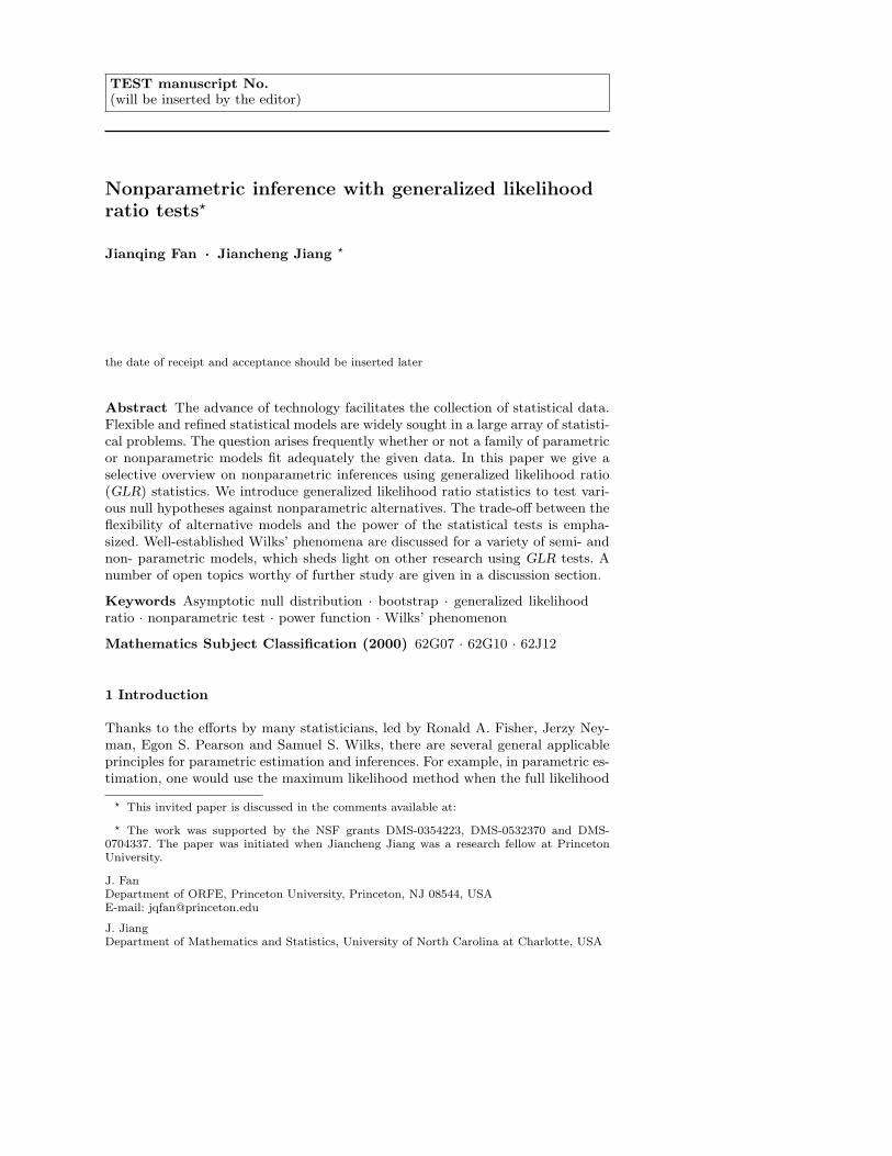
TEST manuscript No. (will be inserted by the editor) Nonparametric inference with generalized likelihood ratio tests ? Jianqing Fan · Jiancheng Jiang ? the date of receipt and acceptance should be inserted later Abstract The advance of technology facilitates the collection of statistical data. Flexible and refined statistical models are widely sought in a large array of statisti- cal problems. The question arises frequently whether or not a family of parametric or nonparametric models fit adequately the given data. In this paper we give a selective overview on nonparametric inferences using generalized likelihood ratio (GLR) statistics. We introduce generalized likelihood ratio statistics to test vari- ous null hypotheses against nonparametric alternatives. The trade-off between the flexibility of alternative models and the power of the statistical tests is empha- sized. Well-established Wilks’ phenomena are discussed for a variety of semi- and non- parametric models, which sheds light on other research using GLR tests. A number of open topics worthy of further study are given in a discussion section. Keywords Asymptotic null distribution · bootstrap · generalized likelihood ratio · nonparametric test · power function · Wilks’ phenomenon Mathematics Subject Classification (2000) 62G07 · 62G10 · 62J12 1 Introduction Thanks to the efforts by many statisticians, led by Ronald A. Fisher, Jerzy Ney- man, Egon S. Pearson and Samuel S. Wilks, there are several general applicable principles for parametric estimation and inferences. For example, in parametric es- timation, one would use the maximum likelihood method when the full likelihood ? This invited paper is discussed in the comments available at: ? The work was supported by the NSF grants DMS-0354223, DMS-0532370 and DMS- 0704337. The paper was initiated when Jiancheng Jiang was a research fellow at Princeton University. J. Fan Department of ORFE, Princeton University, Princeton, NJ 08544, USA E-mail: [email protected] J. Jiang Department of Mathematics and Statistics, University of North Carolina at Charlotte, USA
Transcript of Nonparametric inference with generalized likelihood...
TEST manuscript No.(will be inserted by the editor)
Nonparametric inference with generalized likelihoodratio tests?
Jianqing Fan · Jiancheng Jiang ?
the date of receipt and acceptance should be inserted later
Abstract The advance of technology facilitates the collection of statistical data.Flexible and refined statistical models are widely sought in a large array of statisti-cal problems. The question arises frequently whether or not a family of parametricor nonparametric models fit adequately the given data. In this paper we give aselective overview on nonparametric inferences using generalized likelihood ratio(GLR) statistics. We introduce generalized likelihood ratio statistics to test vari-ous null hypotheses against nonparametric alternatives. The trade-off between theflexibility of alternative models and the power of the statistical tests is empha-sized. Well-established Wilks’ phenomena are discussed for a variety of semi- andnon- parametric models, which sheds light on other research using GLR tests. Anumber of open topics worthy of further study are given in a discussion section.
Keywords Asymptotic null distribution · bootstrap · generalized likelihoodratio · nonparametric test · power function · Wilks’ phenomenon
Mathematics Subject Classification (2000) 62G07 · 62G10 · 62J12
1 Introduction
Thanks to the efforts by many statisticians, led by Ronald A. Fisher, Jerzy Ney-man, Egon S. Pearson and Samuel S. Wilks, there are several general applicableprinciples for parametric estimation and inferences. For example, in parametric es-timation, one would use the maximum likelihood method when the full likelihood
? This invited paper is discussed in the comments available at:
? The work was supported by the NSF grants DMS-0354223, DMS-0532370 and DMS-0704337. The paper was initiated when Jiancheng Jiang was a research fellow at PrincetonUniversity.
J. FanDepartment of ORFE, Princeton University, Princeton, NJ 08544, USAE-mail: [email protected]
J. JiangDepartment of Mathematics and Statistics, University of North Carolina at Charlotte, USA
2
function is available and use the least-squares, generalized method of moments(Hansen, 1982) or generalized estimation equations (Liang and Zeger, 1986) whenonly generalized moment functions are specified. In parametric inferences such ashypothesis testing and construction of confidence regions, the likelihood ratio tests,jackknife, and bootstrap methods (Hall, 1993; Efron and Tibshirani, 1995; Shaoand Tu, 1996) are widely used. The likelihood principle appeared in literature asa term in 1962 (Barnard et al., 1962; Birnbaum, 1962), but the idea goes back tothe works of R.A. Fisher in the 1920s (Fisher, 1922). Since Edwards (1972) cham-pioned the likelihood principle as a general principle of inference for parametricmodels (see also Edwards, 1974), it has been applied to many fields in statistics(see Berger and Wolpert, 1988) and even in the philosophy of science (see Royall,1997).
For nonparametric models, there are also generally applicable methods fornonparametric estimation and modeling. These include local polynomial (Wandand Jones, 1995; Fan and Gijbels, 1996), spline (Wahba, 1990; Eubank, 1999; Gu,2002) and orthogonal series methods (Efromovich, 1999; Vidakovic, 1999), anddimensionality reduction techniques that deal with the issues of the curse of di-mensionality (e.g Fan and Yao, 2003, Chapter 8). On the other hand, while thereare many customized methods for constructing confidence intervals and conduct-ing hypothesis testing (Hart, 1997), there are few generally applicable principlesfor nonparametric inferences. An effort in this direction is Fan, Zhang and Zhang(2001), which extends the likelihood principle by using generalized likelihood ratio(GLR) tests. However, compared with parametric likelihood inference, the GLRmethod is not well developed, and corresponding theory and applications are avail-able only for some models in regression contexts. Therefore, there is a great po-tential for developing the GLR tests, and a review of the idea of GLR inference ismeaningful for encouraging further research on this topic.
Before setting foot in nonparametric inference, we review the basic idea ofparametric inference using the likelihood principle.
1.1 Parametric inference
Suppose that the data generating process is governed by the underlying densityf(x; θ), with unknown θ in a parametric space Θ. The statistical interest lies intesting:
H0 : θ ∈ Θ0 versus H1 : θ ∈ Θ −Θ0
based on a random sample xini=1, where Θ0 is a subspace of Θ. The null hypoth-
esis is typically well formulated. For example, in the population genetics, samplingfrom an equilibrium population with respect to a gene with two alleles (“a” and“A”), three genotypes “AA”, “Aa”, and “aa” can be observed. According to theHardy-Weinberg formula, their proportions are respectively
θ1 = ξ2, θ2 = 2ξ(1− ξ), θ3 = (1− ξ)2.
To test the Hardy-Weinberg formula based on a random sample, the null hypoth-esis is
Θ0 = (θ1, θ2, θ3) : θ1 = ξ2, θ2 = 2ξ(1− ξ), θ3 = (1− ξ)2, 0 ≤ ξ ≤ 1. (1.1)
3
For this problem, we have
Θ = (θ1, θ2, θ3) : θ1 + θ2 + θ3 = 1, 0 ≤ θi ≤ 1.
For such a well formulated question, one can use the well-known maximumlikelihood ratio statistic
λn = 2maxθ∈Θ
`(θ)− maxθ∈Θ0
`(θ),
where `(θ) is the log-likelihood function for getting the given sample under themodel f(x; θ). This is indeed a very intuitive procedure: If the alternative modelsare far more likely to generate the given data, the null models should be rejected.The following folklore theorem facilitates the choice of the critical region: Under H0
and regular conditions, λn is asymptotically chi-square distributed with k degreesof freedom, where k is the difference of dimensions between Θ and Θ0.
An important fundamental property of the likelihood ratio tests is that theirasymptotic null distributions are independent of nuisance parameters in the nullhypothesis such as ξ in (1.1). With this property, one can simulate the null distri-bution by fixing the nuisance parameters at a reasonable value or estimate. Thisproperty is referred to as the Wilk phenomenon in Fan, Zhang and Zhang (2001)and is fundamental to all hypothesis testing problems. It has been a folk theoremin the theory and practice of statistics and has contributed tremendously to thesuccess of the likelihood inference.
In other examples, even though the null hypothesis is well formulated, the al-ternative hypotheses are not. Take the famous model for short-term interest ratesas an example. Under certain assumptions, Cox, Ingersoll and Ross (1985) showedthat the dynamic of short-term rates should follow the stochastic differential equa-tion:
dXt = κ(µ−Xt) dt + σX1/2t dWt, (1.2)
where Wt is a Wiener process on [0,∞), and κ, µ and σ are unknown parameters.This Feller process is called the CIR model in finance. The question arises naturallywhether or not the model is consistent with empirical data. In this case, the nullmodel is well formulated. However, the alternative model is not. To employ theparametric likelihood ratio technique, one needs to embed the CIR model intoa larger family of parametric models such as the following constant elasticity ofvariance model (Chan et al., 1992):
dXt = κ(µ−Xt) dt + σXρt dWt, (1.3)
and test H0 : ρ = 1/2. The drawback of this approach is that the models (1.3)have to include the true data generating process. This is the problem associatedwith all parametric testing problems where it is implicitly assumed that the familyof models f(x; θ) : θ ∈ Θ contains the true one.
To see this more clearly, consider the question if variable X (e.g. age) and Y(salary) are related. If we embed the problem in the linear model
Y = α + βX + ε, (1.4)
4
then the problem becomes testing H0 : β = 0. If unknown to us, the data gener-ating process is govern by
Y = 60− 0.1(X − 45)2 + ε, ε ∼ N(0, 52), (1.5)
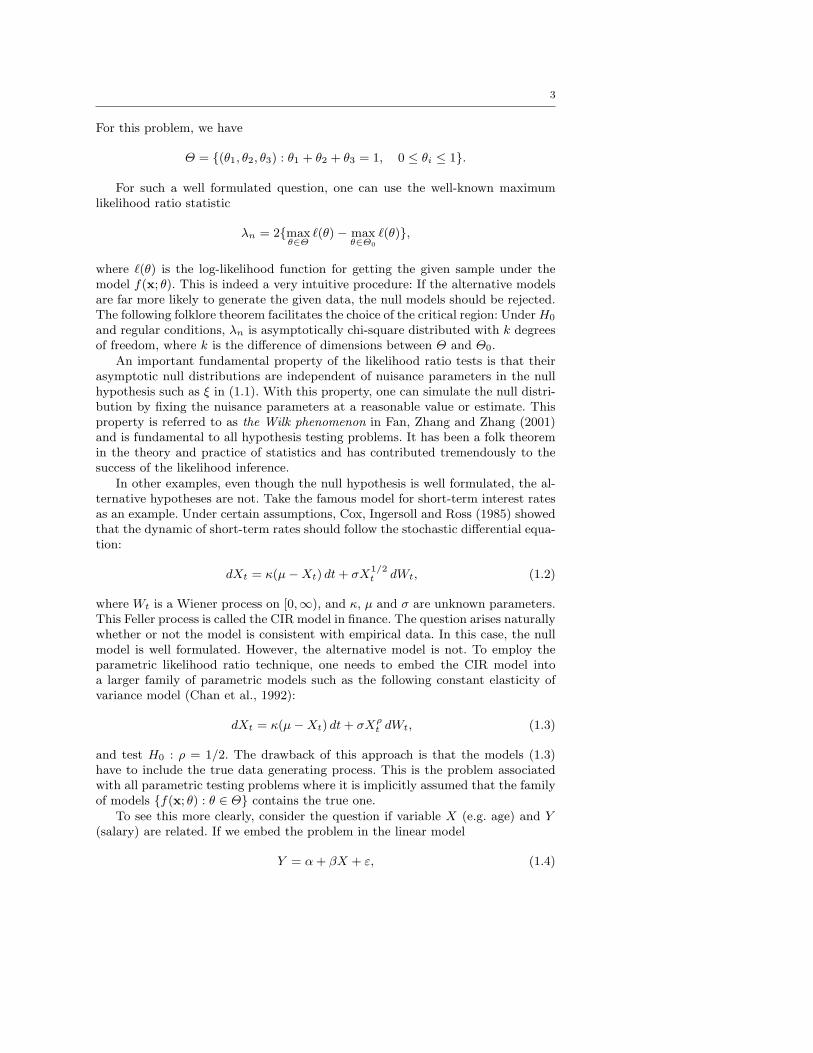
with X uniformly distributed on the interval [25, 65], the null hypothesis will beaccepted very often since slope β in (1.4) is not statistically significant. Figure 1presents a random sample of size 100 from model (1.5). The erroneous conclusionof accepting the null hypothesis is due to the fact that the family of models (1.4)does not contain the true one.
30 40 50 60
2030
4050
60
X
Y
A hypothetical data set
Fig. 1 A simulated data set from (1.5) with sample size 100. When the alternative hypothesisdoes not contain the true model, the fit from the null model (dashed line) is statisticallyindistinguishable from the fit (solid line) from the alternative model (1.4). Erroneous conclusionis drawn from this analysis.
1.2 Nonparametric alternatives
The above discussion reveals that the family of alternative models should be largeenough in order to make sensible inferences. In many hypothesis testing problems,while the null hypothesis is well formulated, the alternative one is vague. These twoconsiderations make nonparametric models as attractive alternative hypothesis.In the hypothetical example presented in Figure 1, without knowing the datagenerating process, a natural alternative model is
Y = m(X) + ε, (1.6)
where m(·) is smooth, while the null hypothesis is Y = µ + ε. This is a paramet-ric null hypothesis against a nonparametric alternative hypothesis. With such aflexible alternative family of models, the aforementioned pitfall is avoided.
5
For the interest rate modeling, a natural alternative to the CIR model (1.2) isthe following one-factor model
dXt = µ(Xt) dt + σ(Xt) dWt,
where µ(·) and σ(·) are unspecified, but smooth functions. This is again the prob-lem of testing a parametric family of models against a nonparametric family ofalternative models. See Fan and Zhang (2003) for a study based on the GLR test.
The problems of nonparametric null against nonparametric alternative hypoth-esis also arise frequently. One may ask if the returns of stock contain jumps or if adiscretely observed process is Markovian. In these cases, both the null and alter-native hypotheses are nonparametric.
The problems of testing nonparametric null against nonparametric alternativehypotheses arise also frequently in statistical inferences. Consider, for example,the additive model (Hastie and Tibshirani, 1990):
Y = α +D∑
d=1
md(Xd) + ε (1.7)
where α is an unknown constant, and md are unknown functions, satisfying E[md(Xdi)]= 0 for identifiability. This nonparametric model includes common multivariatelinear regression models. The question such as if the covariates X1 and X2 arerelated to the response Y arises naturally, which amounts to testing
H0 : m1(·) = m2(·) = 0. (1.8)
This is a nonparametric null versus nonparametric alternative hypothesis testingproblem, since under the null hypothesis (1.8), the model is still a nonparametricadditive model:
Y = α +D∑
d=3
md(Xd) + ε (1.9)
There are many techniques designed to solve this kind of problems. Many ofthem focused on an intuitive approach using discrepancy measures (such as theL2 and L∞ distances) between the estimators under null and alternative mod-els. See early seminal work by Bickel and Rosenblatt (1973), Azzalini, Bowmanand Hardle (1989), and Hardle and Mammen (1993). They are generalizations ofthe Kolmogorov-Smirnov and Cramer-von Mises types of statistics. However, theapproach suffers some drawbacks. First, choices of measures and weights can bearbitrary. Consider, for example, the null hypothesis (1.8) again. The test statisticbased on discrepancy method is T =
∑2d=1 cd‖md‖. One has to choose not only
the norm ‖ · ‖ but the weights cd. Second, the null distribution of the test statisticT is unknown and depends critically on the nuisance functions m3, . . . , mD. Thishampers the applicability of the discrepancy based methods. Naturally, one wouldlike to develop some test methods along the line of parametric likelihood ratiotests that possess Wilks’ phenomenon to facilitate the computation of p-values.
We would like to note that it is possible to design some test statistics thattailored for some specific problems with good power. The question also arisesnaturally if we can come with a generally applicable principle for testing againstnonparametric alternative models. The development of GLR statistics aims at aunified principle for nonparametric hypothesis testing problems.
6
1.3 Flexibility of models and power of tests
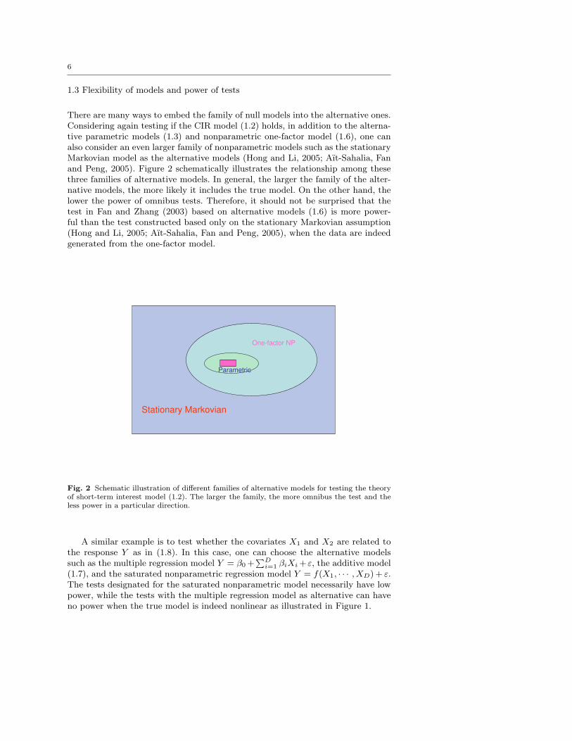
There are many ways to embed the family of null models into the alternative ones.Considering again testing if the CIR model (1.2) holds, in addition to the alterna-tive parametric models (1.3) and nonparametric one-factor model (1.6), one canalso consider an even larger family of nonparametric models such as the stationaryMarkovian model as the alternative models (Hong and Li, 2005; Aıt-Sahalia, Fanand Peng, 2005). Figure 2 schematically illustrates the relationship among thesethree families of alternative models. In general, the larger the family of the alter-native models, the more likely it includes the true model. On the other hand, thelower the power of omnibus tests. Therefore, it should not be surprised that thetest in Fan and Zhang (2003) based on alternative models (1.6) is more power-ful than the test constructed based only on the stationary Markovian assumption(Hong and Li, 2005; Aıt-Sahalia, Fan and Peng, 2005), when the data are indeedgenerated from the one-factor model.
Stationary Markovian
Parametric
One-factor NP
Fig. 2 Schematic illustration of different families of alternative models for testing the theoryof short-term interest model (1.2). The larger the family, the more omnibus the test and theless power in a particular direction.
A similar example is to test whether the covariates X1 and X2 are related tothe response Y as in (1.8). In this case, one can choose the alternative modelssuch as the multiple regression model Y = β0 +
∑Di=1 βiXi +ε, the additive model
(1.7), and the saturated nonparametric regression model Y = f(X1, · · · , XD) + ε.The tests designated for the saturated nonparametric model necessarily have lowpower, while the tests with the multiple regression model as alternative can haveno power when the true model is indeed nonlinear as illustrated in Figure 1.
7
1.4 Organization of the paper
In Section 2, we discuss some drawbacks of the naive extension of classical maxi-mum likelihood ratio tests to nonparametric setting. Section 3 outlines the frame-work for the GLR tests. Several established Wilk’s type of results for variousnonparametric models are summarized in Section 4. In Section 5, we conclude thispaper and set forth some open problems.
2 Naive extension of maximum likelihood ratio tests
Although likelihood ratio theory contributes tremendous success to parametric in-ference, there are few general applicable approaches for nonparametric inferencesbased on function estimation. A naive extension is the nonparametric maximumlikelihood ratio test. However, nonparametric maximum likelihood estimation usu-ally does not exist. Even if it exists, it is hard to compute. Furthermore, theresulting maximum likelihood ratio tests are not optimal.
The following example from Fan, Zhang and Zhang (2001) illustrates the abovepoints and provides additional insights.
2.1 Problems with nonparametric maximum likelihood ratio tests
Suppose that there are n data points (Xi, Yi) sampled from the following model:
Yi = m(Xi) + εi, i = 1, . . . , n, (2.10)
where εi is a sequence of i.i.d. random variables from N (0, σ2) and Xi has adensity with compact support, say [0, 1]. Assume that the parametric space is
Fk =m ∈ L2[0, 1] :
∫ 1
0[m(k)(x)]2 dx ≤ C
,
for a given constant C. Consider the testing problem:
H0 : m(x) = α0 + α1x versus H1 : m(x) 6= α0 + α1x. (2.11)
Then the conditional log-likelihood function is
`(m, σ) = −n log(√
2πσ)− 1
2σ2
n∑
i=1
(Yi −m(Xi))2. (2.12)
Denote by (α0, α1) the maximum likelihood estimator (MLE) under H0, andmMLE(·) the MLE under Fk which solves the following minimization problem:
minn∑
i=1
(Yi −m(Xi))2, subject to
∫ 1
0m(k)(x)2 dx ≤ C.
Then mMLE is a smoothing spline (Wahba, 1990; Eubank, 1999) with the smooth-
ing parameter chosen to satisfy ||m(k)MLE||22 = C. Define the residual sum of squares
under the null and alternative as follows:
RSS0 =n∑
i=1
(Yi − α0 − α1Xi)2, RSS1 =
n∑
i=1
(Yi − mMLE(Xi))2.
8
Then the logarithm of the conditional maximum likelihood ratio statistic for thetesting problem (2.11) is given by
λn = `(mMLE, σ)− `(m0, σ0) =n
2log
RSS0
RSS1,
where σ2 = n−1RSS1, m0(x) = α0 + α1x, and σ20 = n−1RSS0.
Even in this simple situation where the nonparametric maximum likelihoodexists, we need to know the constant C in the parametric space Fk in order tocompute the MLE. This is unrealistic in practice. Even if the value C is granted,Fan, Zhang and Zhang (2001) demonstrated (see also §2.2) that the nonparametricmaximum likelihood ratio test is not optimal. This is due to the limited choice of
smoothing parameter in mMLE, which makes it satisfy ||m(k)MLE||22 = C. In this
case, the essence of the testing problem is to estimate the functional ‖m‖2 (weassume that α0 = α1 = 0 in (2.11) without loss of generality as they can beestimated faster than nonparametric rates). It is well-known that one smoothingparameter can not optimize simultaneously the estimate of the functional ‖m‖2and the function m(·). See for example, Bickel and Ritov (1988); Hall and Marron(1988); Donoho and Nussbaum (1990); Fan (1991).
Now, if the parameter space is F ′k = m ∈ L2[0, 1] : sup0≤x≤1 |m(k)(x)| ≤C or more complicated space, it is not clear whether the maximum likelihoodestimator exists and even if it exists, how to compute it efficiently.
The above example reveals that the nonparametric MLE may not exist andhence cannot serve as a generally applicable method. It illustrates further that,even when it exists, the nonparametric MLE chooses smoothing parameters au-tomatically. This is too restrictive for the procedure to possess the optimality oftesting problems. Further, we need to know the nonparametric space exactly. Forexample, the constant C in Fk needs to be specified. The GLR statistics in Fan,Zhang and Zhang (2001), which replaces the nonparametric maximum likelihoodestimator by any reasonable nonparametric estimator, attenuate these difficultiesand enhances the flexibility of the test statistic by varying the smoothing pa-rameter. By proper choices of the smoothing parameter, the GLR tests achievethe optimal rates of convergence in the sense of Ingster (1993) and Lepski andSpokoiny (1999).
2.2 Inefficiency of nonparametric maximum likelihood ratio tests
To demonstrate the inefficiency of nonparametric maximum likelihood ratio tests,let us consider a simpler mathematical model, the Gaussian white noise model, tosimplify the technicality of mathematical proofs. The model keeps all importantfeatures of nonparametric regression model, as demonstrated by Brown and Low(1996) and Grama and Nussbaum (2002). Suppose that we have observed thewhole process Y (t) from the following Gaussian white noise model:
dY (t) = φ(t) dt + n−1/2 dW (t), t ∈ (0, 1), (2.13)
where φ is an unknown function and W (t) is the Brownian process. By using anorthogonal series (e.g. the Fourier series) transformation, model (2.13) is equivalent
9
to the following white noise model:
Yi = θi + n−1/2εi, εiiid∼ N (0, 1), i = 1, 2, . . .
where Yi, θi and εi are the i-th Fourier coefficients of Y (t), φ(t) and W (t), respec-tively. Now let us consider testing the simple hypothesis:
H0 : θ1 = θ2 = · · · = 0, (2.14)
which is equivalent to testing H0 : φ = 0 under model (2.13).Consider the parametric space F∗k = θ :
∑∞j=1 j2kθ2
j ≤ 1 where k ≥ 0.When k is a positive integer, this set in the frequency domain is equivalent to theSobolev class of periodic functions φ : ||φ(k)|| ≤ c for a constant c. Then underthe parameter space F∗k , the maximum likelihood estimator is
θj = (1 + ξj2k)−1Yj ,
where ξ is the Lagrange multiplier satisfying
∞∑
j=1
j2kθ2j = 1. (2.15)
Under the null hypothesis (2.14), Lemma 2.1 of Fan, Zhang and Zhang (2001)shows that
ξ = n−2k/(2k+1)∫ ∞
0
y2k
(1 + y2k)2dy
2k/(2k+1)1 + op(1).
The maximum likelihood ratio statistic for the problem (2.14) is
λ∗n =n
2
∞∑
j=1
(1− j4kξ2
(1 + j2kξ)2
)Y 2
j .
Fan, Zhang and Zhang (2001) proved that the maximum likelihood ratio test,λ∗n, can test consistently alternatives with a rate no faster than n−(k+d)/(2k+1)
for any d > 1/8. Theorefore, when k > 1/4, by taking d sufficiently close to 1/8,the test λ∗n cannot be optimal according to the formulations of Ingster (1993) forhypothesis testing where an optimal test can detect alternatives converging to thenull with rate n−2k/(4k+1). This is due to the restrictive choice of the smoothingparameter ξ of the MLE, which has to satisfy (2.15). GLR tests remove this re-strictive requirement and allow one to tune optimally the smoothing parameter.By taking ξn = cn−4k/(4k+1) for some c > 0, the GLR test statistic defined by
λn =n
2
∞∑
j=1
(1− j4kξ2
n
(1 + j2kξn)2
)Y 2
j ,
achieves the optimal rate of convergence for hypothesis testing (Theorem 3 of Fan,Zhang and Zhang, 2001).
The GLR test allows one to use any reasonable nonparametric estimator toconstruct the test. For the Sobolev class F∗k , another popular class of nonpara-metric estimator is the truncation estimator (see Efromovich, 1999):
θj = Yj , for j = 1, · · · , m, θj = 0, for j > m,
10
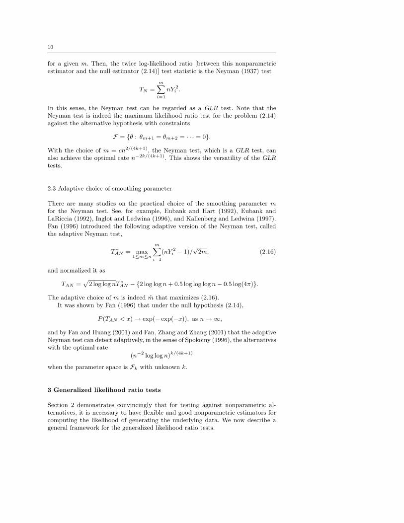
for a given m. Then, the twice log-likelihood ratio [between this nonparametricestimator and the null estimator (2.14)] test statistic is the Neyman (1937) test
TN =m∑
i=1
nY 2i .
In this sense, the Neyman test can be regarded as a GLR test. Note that theNeyman test is indeed the maximum likelihood ratio test for the problem (2.14)against the alternative hypothesis with constraints
F = θ : θm+1 = θm+2 = · · · = 0.
With the choice of m = cn2/(4k+1), the Neyman test, which is a GLR test, canalso achieve the optimal rate n−2k/(4k+1). This shows the versatility of the GLRtests.
2.3 Adaptive choice of smoothing parameter
There are many studies on the practical choice of the smoothing parameter mfor the Neyman test. See, for example, Eubank and Hart (1992), Eubank andLaRiccia (1992), Inglot and Ledwina (1996), and Kallenberg and Ledwina (1997).Fan (1996) introduced the following adaptive version of the Neyman test, calledthe adaptive Neyman test,
T ∗AN = max1≤m≤n
m∑
i=1
(nY 2i − 1)/
√2m, (2.16)
and normalized it as
TAN =√
2 log log nT ∗AN − 2 log log n + 0.5 log log log n− 0.5 log(4π).
The adaptive choice of m is indeed m that maximizes (2.16).It was shown by Fan (1996) that under the null hypothesis (2.14),
P (TAN < x) → exp(− exp(−x)), as n →∞,
and by Fan and Huang (2001) and Fan, Zhang and Zhang (2001) that the adaptiveNeyman test can detect adaptively, in the sense of Spokoiny (1996), the alternativeswith the optimal rate
(n−2 log log n)k/(4k+1)
when the parameter space is Fk with unknown k.
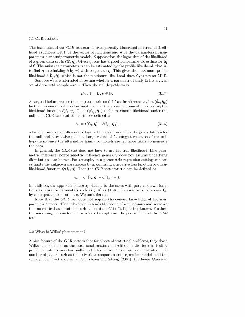
3 Generalized likelihood ratio tests
Section 2 demonstrates convincingly that for testing against nonparametric al-ternatives, it is necessary to have flexible and good nonparametric estimators forcomputing the likelihood of generating the underlying data. We now describe ageneral framework for the generalized likelihood ratio tests.
11
3.1 GLR statistic
The basic idea of the GLR test can be transparently illustrated in terms of likeli-hood as follows. Let f be the vector of functions and η be the parameters in non-parametric or semiparametric models. Suppose that the logarithm of the likelihoodof a given data set is `(f , η). Given η, one has a good nonparametric estimator fηof f . The nuisance parameters η can be estimated by the profile likelihood, that is,to find η maximizing `(fη , η) with respect to η. This gives the maximum profile
likelihood `(fη , η), which is not the maximum likelihood since fη is not an MLE.Suppose we are interested in testing whether a parametric family fθ fits a given
set of data with sample size n. Then the null hypothesis is
H0 : f = fθ, θ ∈ Θ. (3.17)
As argued before, we use the nonparametric model f as the alternative. Let (θ0, η0)be the maximum likelihood estimator under the above null model, maximizing thelikelihood function `(fθ, η). Then `(fθ0
, η0) is the maximum likelihood under thenull. The GLR test statistic is simply defined as
λn = `(fη , η)− `(fθ0, η0), (3.18)
which calibrates the difference of log-likelihoods of producing the given data underthe null and alternative models. Large values of λn suggest rejection of the nullhypothesis since the alternative family of models are far more likely to generatethe data.
In general, the GLR test does not have to use the true likelihood. Like para-metric inference, nonparametric inference generally does not assume underlyingdistributions are known. For example, in a parametric regression setting one canestimate the unknown parameters by maximizing a negative loss function or quasi-likelihood function Q(fθ, η). Then the GLR test statistic can be defined as
λn = Q(fη , η)−Q(fθ0, η0).
In addition, the approach is also applicable to the cases with part unknown func-tions as nuisance parameters such as (1.8) or (1.9). The essence is to replace fθ0
by a nonparametric estimate. We omit details.Note that the GLR test does not require the concise knowledge of the non-
parametric space. This relaxation extends the scope of applications and removesthe impractical assumptions such as constant C in (2.11) being known. Further,the smoothing parameter can be selected to optimize the performance of the GLRtest.
3.2 What is Wilks’ phenomenon?
A nice feature of the GLR tests is that for a host of statistical problems, they shareWilks’ phenomenon as the traditional maximum likelihood ratio tests in testingproblems with parametric nulls and alternatives. These are demonstrated in anumber of papers such as the univariate nonparametric regression models and thevarying-coefficient models in Fan, Zhang and Zhang (2001), the linear Gaussian
12
process in Fan and Zhang (2004) for spectral density estimation, the varying-coefficient partly linear models in Fan and Huang (2005), the additive models inFan and Jiang (2005), the diffusion models in Aıt-Sahalia, Fan and Peng (2005),and the partly linear additive models in Jiang et al (2007). Corresponding results indepth will be given in Section 4. These results indicate that the Wilks phenomenaexist in general.
By Wilks’ phenomenon, we mean that the asymptotic null distributions oftest statistics are independent of nuisance parameters and functions. Typically,the asymptotic null distribution of the GLR statistic λn is nearly χ2 with largedegrees of freedom in the sense that
rλnd' χ2
µn(3.19)
for a sequence µn →∞ and a constant r, namely,
(2µn)−1/2(rλn − µn)L→ N (0, 1),
where µn and r are independent of nuisance parameters/functions. They maydepend on the methods of nonparametric estimation and smoothing parameters.Therefore, the asymptotic null distribution is independent of the nuisance pa-rameters/functions. With this Wilks phenomenon, the advantages of the classicallikelihood ratio tests are fully inherited: one makes a statistical decision by com-paring likelihoods of generating the given data under two competing classes ofmodels and the critical value can easily be found based on the known null distri-bution N (µn, 2µn) or χ2
µn. Another important consequence of the results is that
one does not have to derive theoretically the constant µn and r in order to use theGLR tests, since as long as there is such a Wilks type of phenomenon, one cansimply simulate the null distributions by setting nuisance parameters under thenull hypothesis at reasonable values or estimates.
The above Wilks phenomenon is not a coincidence for the nonparametricmodel. In the exponential family of models with growing number of parameters,Portnoy (1988) showed the Wilks type of result in the same sense as (3.19), andMurphy (1993) revealed a similar type of result for Cox’s proportional hazardsmodel using a simple sieve method (piecewise constant approximation to a smoothfunction). While there is no general theory on the GLR tests, various authors havedemonstrated that Wilks’ phenomenon holds for many nonparametric models (seeSection 4).
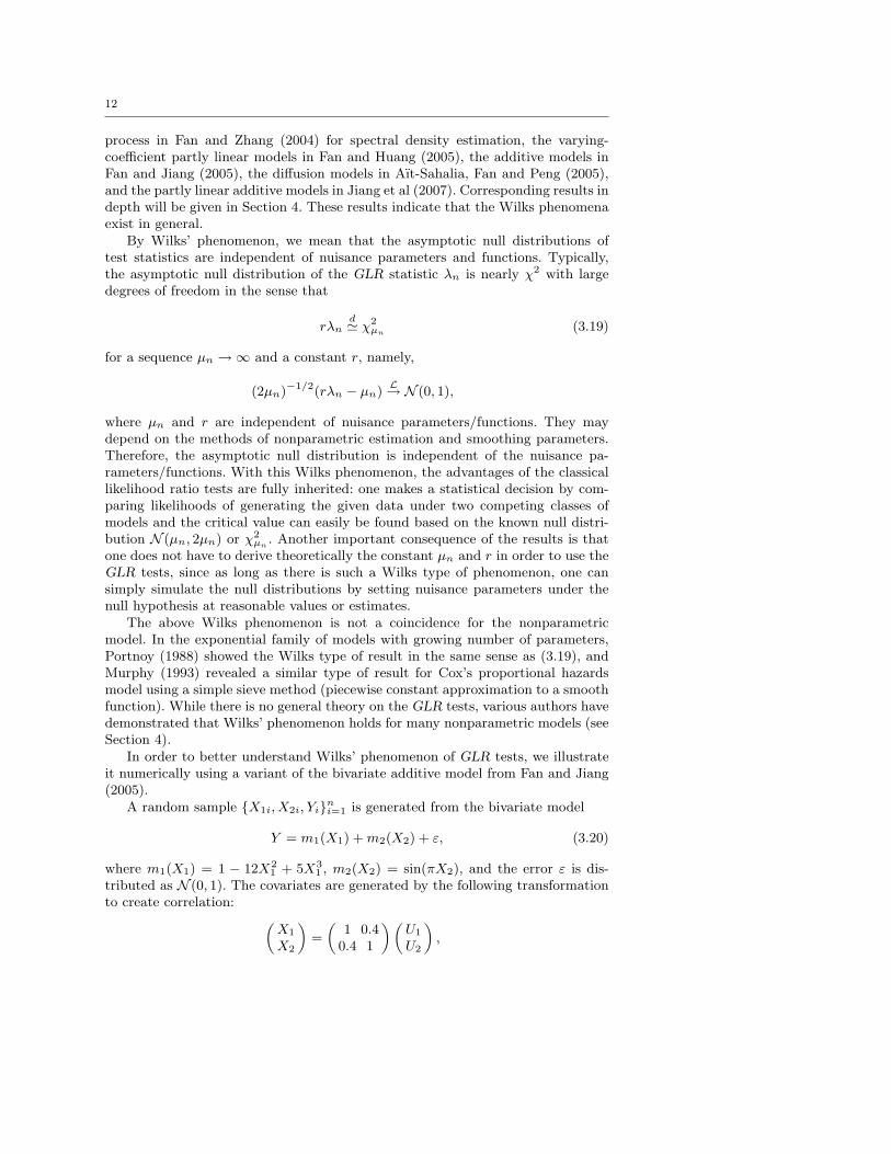
In order to better understand Wilks’ phenomenon of GLR tests, we illustrateit numerically using a variant of the bivariate additive model from Fan and Jiang(2005).
A random sample X1i, X2i, Yini=1 is generated from the bivariate model
Y = m1(X1) + m2(X2) + ε, (3.20)
where m1(X1) = 1 − 12X21 + 5X3
1 , m2(X2) = sin(πX2), and the error ε is dis-tributed as N (0, 1). The covariates are generated by the following transformationto create correlation:
(X1
X2
)=
(1 0.4
0.4 1
) (U1
U2
),
13
0 5 10 150
0.05
0.1
0.15
0.2
0 5 10 150
0.05
0.1
0.15
0.2
0 5 10 150
0.05
0.1
0.15
0.2
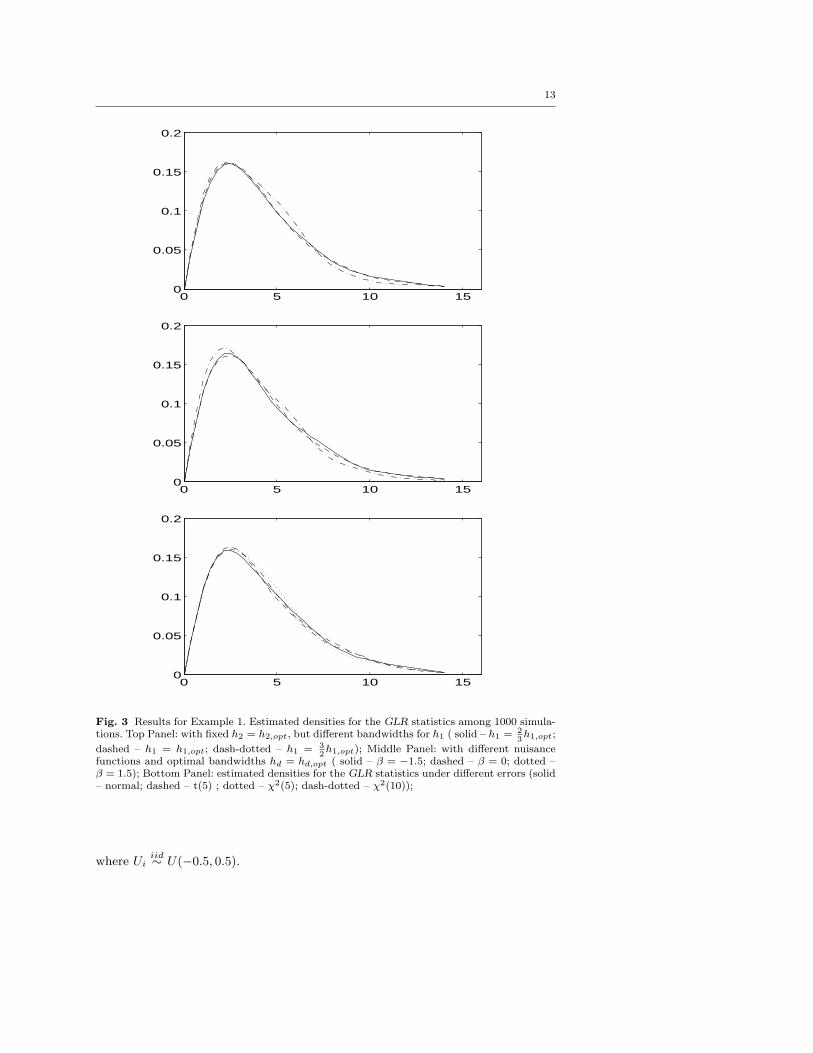
Fig. 3 Results for Example 1. Estimated densities for the GLR statistics among 1000 simula-tions. Top Panel: with fixed h2 = h2,opt, but different bandwidths for h1 ( solid – h1 = 2
3h1,opt;
dashed – h1 = h1,opt; dash-dotted – h1 = 32h1,opt); Middle Panel: with different nuisance
functions and optimal bandwidths hd = hd,opt ( solid – β = −1.5; dashed – β = 0; dotted –β = 1.5); Bottom Panel: estimated densities for the GLR statistics under different errors (solid– normal; dashed – t(5) ; dotted – χ2(5); dash-dotted – χ2(10));
where Uiiid∼ U(−0.5, 0.5).
14
Consider the testing problem:
H0 : m2(x2) = 0 versus H1 : m2(x2) 6= 0.
Since m1(·) is an unknown nuisance function, this testing problem is actuallya nonparametric null hypothesis against a nonparametric alternative hypothesis.Frequently, the backfitting algorithm with a smoothing method (Hastie and Tib-shirani, 1990) is employed to estimate the additive components in (3.20). We hereemploy the backfitting algorithm with the local linear smoother using bandwidthh1 for estimating m1 and h2 for estimating m2 to construct a GLR statistic. SeeSection 4.5 for additional details.
To demonstrate Wilks’ phenomenon for the GLR test, we use (i) three levels ofbandwidth h1 = 2
3h1,opt, h1,opt, or 32h1,opt with h2 fixed at its optimal value h2,opt,
where hd,opt is the optimal bandwidth for the smoother on md(·) (see Opsomer,2000); and (ii) three levels of nuisance function m1(X1):
m1,β(X1) =
[1 + β
√var(0.5− 6X2
1 + 3X31 )
](0.5− 6X2
1 + 3X31 ),
where β = −1.5, 0, 1.5. For the GLR test, we drew 1000 samples of 200 obser-vations. Based on the 1000 samples, we obtained 1000 GLR test statistics. Theirdistribution is obtained via a kernel estimate with a rule of thumb bandwidth:h = 1.06sn−0.2, where s is the standard deviation of the normalized GLR statis-tics.
Figure 3 shows the estimated densities of the normalized GLR statistics, rλn,where r is the normalization constant given in Section 4.5. As expected, they looklike densities from χ2-distributions. The top panel of Figure 3 shows that thenull distributions follow χ2-distributions over a wide range of bandwidth h1. Notethat different bandwidths h1 gives different complexity of modeling the nuisancefunction m1 and the results show that the null distributions are nearly independentof the different model complexity of the nuisance function m1. This demonstratesnumerically Wilks’ phenomenon. Note that the degree of freedom depends onbandwidth h2 but not on h1, which reflects the difference of the complexity of m2
under the null model and the alternative model.The middle panel demonstrates also the Wilks type of phenomenon from a
different angle: for the three very different choices of nuisance functions, the nulldistributions are nearly the same.
To investigate the influence of different noise distributions on the GLR tests,we now consider model (3.20) with different error distributions of ε. In additionto the standard normal distribution, the standardized t(5) and the standardizedχ2(5) and χ2(10) are also used to assess the stability of the null distributionof the GLR test for different error distributions. The bottom panel of Figure 3reports the estimated densities of the normalized GLR statistics under the abovefour different error distributions. It shows that the null distributions of the testsare approximately the same for different error distributions, which again endorsesWilks’ phenomenon.
3.3 Choice of smoothing parameter
The GLR statistic involves at least a parameter h in smoothing the function f .For each given smoothing parameter h, the GLR statistic λn(h) is a test statistic.
15
This forms a family of test statistics indexed by h. In general, a larger choice ofbandwidth is more powerful for testing smoother alternatives, and a smaller choiceof bandwidth is more powerful for testing less smooth alternatives. Questions ariseabout how to choose a bandwidth for nonparametric testing and what criteriashould be used.
Assume that the Wilks type of result (3.19) holds with degree of freedomµn(h). Inspired by the adaptive Neyman test (2.16) of Fan (1996), which achievesthe adaptive optimal rate, an adaptive choice of bandwidth is to maximize thenormalized test statistic
h = arg maxh∈[n−a,n−b]
rλn(h)− µn(h)/√
2µn(h),
for some a, b > 0. This results in the following multiscale GLR test statistic inFan, Zhang and Zhang (2001),
maxh∈[n−a,n−b]
rλn(h)− µn(h)/√
2µn(h). (3.21)
Like the adaptive optimality of the adaptive Neyman test, it is expected that themulti-scale GLR test possesses a similar optimality property. Indeed, Horowitz andSpokoiny (2001, 2002) demonstrated this kind of property for two specific models.
In practical implementations, one needs only to find the maximum in the mul-tiscale GLR test (3.21) over a grid of bandwidths. Zhang (2003a) calculated thecorrelation between λn(h) and λn(ch) for some inflation factor c. The correlationis quite large when c = 1.3. Thus, a simple implementation is to choose a gridof points h = h01.5j for j = −1, 0, 1, representing “small”, “right”, and “large”bandwidths. A natural choice of h0 is the optimal bandwidth in the function esti-mation.
Another choice of bandwidth is to choose an optimal bandwidth to maximizethe power of the GLR test over some specific family of alternative models. Thisproblem has not been seriously explored in the literature. For practical implemen-tations, the bandwidth used for curve fitting provides a reasonable starting pointfor the GLR tests, although it may not optimize the power. In general, there is nobig difference in rates for the optimal bandwidths for estimation and testing. Infact, the optimal bandwidth for the local linear estimation of a univariate f is of or-der O(n−1/5), and that for the GLR test is of order O(n−2/9) = O(n−1/5×n−1/45).Therefore, with the estimated optimal bandwidth h for estimation, one can employthe ad hoc bandwidth, h× n−1/45, for the GLR test.
3.4 Bias correction
When fθ in the null hypothesis in (3.17) is not linear/polynomial, a local linear/polyno-mial fit will result in a biased estimate under the null hypothesis. Similarly, whenthe function fθ is not a spline function, the spline based smoothing results in thebias of the estimate under the null hypothesis. These affect the precision of nulldistribution of the GLR statistic and hence the reliability of statistical conclusion.
The aforementioned bias problem can be significantly attenuated as follows.Reparameterize the unknown functions as f∗ = f − fθ0
. Then the test problem
16
(3.17) becomes testing
H0 : f∗ = 0 versus f∗ 6= 0
with the likelihood or more generally the quasi-likelihood function Q∗(f∗, η) =Q(f∗ + fθ0
, η). Applying the GLR test to this reparameterized problem with thenew quasi-likelihood function Q∗(f∗, η), one can eliminate the bias problem inthe null distribution, since any reasonable nonparametric estimator will not havebiases when the true function is zero. Let (f
∗η , η) be a profile estimator based on
Q∗(f∗, η). Then the bias-corrected version of the GLR test is
T ∗ = Q∗(f∗η , η)−Q∗(0, η0) = Q(f
∗η + fθ0
, η)−Q(fθ0, η0)
The above idea is inspired by the prewhitening technique of Press and Tukey(1956) in spectral density estimation and the technique that was employed byHardle and Mammen (1993) for univariate nonparametric testing. Indeed, for theunivariate regression setting, our general method coincides with the test in Hardleand Mammen (1993). Our method is also related to the nonparametric estimatorthat uses a parametric start of Hjort and Glad (1995) and Glad (1998). Recently,Fan and Zhang (2004) and Fan and Jiang (2005) advocated the use of the biasreduction method in the study of testing problems for spectral density and additivemodels, respectively, when the null hypothesis is a parametric family.
3.5 Bootstrap
To implement a GLR test, we need to obtain the null distribution of the test statis-tic. Theoretically the asymptotic null distribution in (3.19) can be used in deter-mining the p-value of a GLR statistic. However, this needs to derive its asymptoticnull distribution. In addition, the asymptotic distribution does not necessarily givea good approximation for finite sample sizes. For example, from the asymptoticpoint of view, the χ2
µn+100-distribution and the χ2µn
-distribution are approximatelythe same since µn →∞, but for moderate µn, they are quite different. This meansthat a second order term is needed. Assume that the appropriate degree of freedomis µn + c for a constant c. Then when the bandwidth is large (h → ∞), the locallinear fit becomes a global linear fit, and the GLR test becomes the parametricmaximum likelihood ratio test. Hence, λn → χ2
2p in distribution according to theclassic Wilks type of result, where 2p denotes the difference of the degree of free-dom difference under the null and alternative hypothesis. It is reasonable to expectthat the degree of freedom µn + c → 2p as h →∞. Since typically µn depends onh in such a way that µn → 0 as h → ∞, we have c = 2p. This is the calibrationidea in Zhang (2003b). However, it also may not lead to a good approximation tothe null distribution of λn, since in most of cases the bandwidth h is not so bigand the above calibration method may fail.
Thanks to Wilks’ phenomenon for the GLR test statistic, the asymptotic nulldistribution is independent of nuisance parameters/functions under the null hy-pothesis. For a finite sample, this means that the null distribution does not sensi-tively depend on the nuisance parameters/functions. Therefore, the null distribu-tion can be approximated by simulations, via fixing nuisance parameters/functionsat their reasonable estimates. Since the resampling approximation is generally wild
17
bootstrap, the resulting estimator of the null distribution is consistent. For dif-ferent settings, some bootstrap approximations to the null distributions of GLRstatistics have been studied. For details, see Section 4.
An additional advantage of the bootstrap method is that one does not needto derive the asymptotic null distribution first. As long as Wilks’ phenomenon isbelieved to be true, it provides a consistent estimate of the null distribution.
3.6 Power
In various settings, it has been shown that the GLR tests are asymptoticallyoptimal in the sense that they can detect alternatives with optimal rates for non-parametric hypothesis testing according to the formulation of Ingster (1993) andLepski and Spokoiny (1999). The optimality here is not the same as the uniformlymost powerful (UMP) test in the classic sense. In fact, for problems as complexas ours, no UMP test exists.
For the testing problem in (3.17), one may consider the following contiguousalternatives
H1n : f = fθ + n−γgn,
where γ > 0 and gn is an unspecified vector sequence of smooth functions in alarge class of functions. The power of the GLR test under the above alternativehas been investigated by several authors for different models, see for example Fan,Zhang and Zhang (2001) and Fan and Jiang (2005) among others. In general, itcan be shown that when the local linear smoother is employed for estimating f andthe bandwidth is of order n−2/9, the GLR test can detect alternatives with therate γ = 4/9 which is optimal according to Ingster (1993). Thus, the generalizedlikelihood method is not only intuitive to use, but also powerful to apply. Thislends further support for the use of the generalized likelihood method.
4 Wilks’ phenomena
In the last section, we introduced a general framework of the GLR test and itsvarious implementation. The approach is general and can be used in many non-parametric testing problems. In the following, we present some established Wilkstype of results for various models. This provides a stark evidence for the versatilityof the results, which in terms supports the methodology.
4.1 Nonparametric regression
Consider the following nonparametric model
Yi = m(Xi) + εi, i = 1 . . . , n, (4.22)
where εi are iid random variables such that E(εi) = 0 and var(εi) = σ2. The uni-variate nonparametric regression model (4.22) is one of the simplest nonparametricmodels for understanding nonparametric techniques. It has been exhaustedly stud-ied in the literature. Enormous papers have been devoted to the estimation and
18
inference of the univariate regression model and it is impossible to mention all ofthe related references. See the references in the books mentioned in the secondparagraph of the introduction for further details.
We now apply the GLR test to the testing problem
H0 : m(x) = α0 + α1x versus H1 : m(x) 6= α0 + α1x,
where α0 and α1 are unknown parameters. Using the local linear fit with a kernelK and a bandwidth h, one can obtain the estimator mh(·) of the unknown functionm(·) under the full model. If the error is normal, then the log-likelihood function`(m, σ) is given by (2.12). Substituting the nonparametric estimator mh(·) intothe likelihood function, we obtain the likelihood of generating the collected sampleunder the nonparametric model as
`(mh, σ) = −n log(√
2πσ)− 1
2σ2RSS1, (4.23)
where RSS1 =∑n
i=1(Yi − mh(Xi))2. Maximizing the above likelihood with re-
spect to σ2 yields σ2 = n−1RSS1. Substituting the estimate into (4.23) gives thelikelihood,
`(mh, σ) = −n
2log(RSS1)− n
2[1 + log(2π/n)].
Denote by (a0, α1) the least squares estimator of (α0, α1), and define RSS0 =∑ni=1(Yi − α0 − α1Xi)
2. Using a similar argument as above, we get the likelihoodunder H0 as
`(m0, σ0) = −n
2log(RSS0)− n
2[1 + log(2π/n)].
Thus, the GLR statistic in (3.18) for the above testing problem is
λn,1 = `(mh, σ)− `(m0, σ0) =n
2log(RSS0/RSS1). (4.24)
Under the null hypothesis and certain conditions, if nh3/2 → ∞, the Wilkstype of result holds (Fan, Zhang and Zhang, 2001, Section 4.1)
rKλn,1a∼ χ2
µn, (4.25)
where µn = rKcK |Ω|/h with |Ω| denoting the Lebesgue’s measure of the supportof X, rK = cK/dK with cK = K(0)− 0.5‖K‖2 and dK = ‖K − 0.5K ∗K‖2.
The above result demonstrates that the GLR statistic obeys Wilks’ phenomenonin this simple setup — the asymptotic null distribution is independent of any nui-sance parameters, such as σ2 and the density function of the covariate X. Thenormalization factor is rK rather than 2 in the parametric maximum likelihoodratio test. The degrees of freedom depend on |Ω|/h, the difference of the effec-tive number of parameters used under the null and alternative hypotheses. Thiscan be understood as follows. Suppose that we partition the support of X intoequispaced intervals, each with length h. This results in |Ω|/h intervals. Hence,the difference of the number of parameters between the null and the alternativeis approximately proportional to |Ω/h|. Since the local linear smoother uses over-lapping intervals, the effect number of parameters is slightly different from |Ω/h|.The constant factor rKcK reflects this difference.
Based on Wilks’ phenomenon, the null distribution of the GLR statistic canbe estimated by using the following conditional bootstrap method:
19
(1) Obtain the parametric estimates α0 and α1 and nonparametric estimate m(x)under both the null and the alternative models. Fix the bandwidth at itsestimated value h in the estimation stage.
(2) Compute the GLR test statistic λn,1 and the residuals εi from the nonpara-metric model (for a given data set, we are not certain whether the null modelholds, so we use the fits from the larger alternative model, which is consistentunder both classes of models).
(3) For each Xi, draw a bootstrap residual ε∗i from the centered empirical dis-tribution of εi and compute Y ∗i = α0 + α1Xi + ε∗i . This forms a conditionalbootstrap sample Xi, Y
∗i n
i=1.(4) Use the above bootstrap sample to construct the GLR statistic λ∗n,1.(5) Repeat Steps 3 and 4 B times (say B=1,000) and obtain B values of the statistic
λ∗n,1.(6) Use the B values in Step 5 to determine the quantiles of the test statistic under
H0. The p-value is simply the percentage of λ∗n,1 values greater than λn,1.
The above resampling approximation method is the wild bootstrap. Using thesame argument as in Fan and Jiang (2005), one can establish the consistency ofthe above conditional bootstrap estimation.
Consider now more generally the testing problem
H0 : m(x) = m(x; θ) versus H1 : m(x) 6= m(x; θ). (4.26)
When m(x; θ) is non-linear, the local linear estimate is biased. The result (4.25)does not hold unless the bandwidth h is small enough (e.g., h = o(n−2/9); seeFan, Zhang and Zhang, 2001). The bias correction method in §3.4 is to apply thelocal linear smoother to the data (Xi, Yi −m(Xi; θ)), i = 1, · · · , n to obtain theestimator m∗
h(·) using a kernel K with the bandwidth h. When the null hypothesisin (4.26) holds, the conditional mean function of Yi−m(Xi; θ) given Xi is approx-imately zero and hence the local linear estimator does not introduce much biases.With the transformation outlined in §3.4, the log-likelihoods under the null andalternative models are the same as before, except RSS0 and RSS1 now replacedby
RSS∗0 =n∑
i=1
(Yi −m(Xi; θ))2, RSS∗1 =
n∑
i=1
(Yi −m(Xi; θ)− m∗h(Xi))
2.
The GLR statistic with bias correction now becomes (see also (4.24)) λ∗n,1
= n2 log(RSS∗0/RSS∗1). The result (4.25) continues to hold for the bias-corrected
GLR statistic λ∗n,1. The procedure is in the same spirit as that used in Hardle andMammen (1993).
4.2 Varying-coefficient models
The varying-coefficient models arise in many statistical problems. They have beensuccessfully applied to nonlinear time series models (Haggan and Ozaki, 1981;Chen and Tsay, 1993; Fan, Yao and Cai, 2003; Fan and Yao, 2003), the multi-dimensional nonparametric regression (Cleveland, Grosse and Shyu, 1991; Hastieand Tibshirani, 1993; Fan and Zhang, 1999) and generalized linear models (Kauer-mann and Tutz, 1999; Cai, Fan and Li, 2000). They have also been widely used in
20
the analysis of longitudinal and functional data (Brumback and Rice, 1998; Car-rol, Ruppert and Welsh, 1998; Hoover et al., 1998; Huang, Wu and Zhou, 2002;Fan and Li, 2004) and financial modeling (Hardle, Herwartz and Spokoiny, 2003;Mercurio and Spokoiny, 2004).
In the multiple nonparametric regression, the varying-coefficient model as-sumes
Y = a1(U)X1 + · · ·+ ap(U)Xp + ε,
where ε is independent of covariates (U, X1, . . . , Xp) and has mean zero and vari-ance σ2. It provides a useful tool for capturing possible nonlinear interactionsamong covariates X and U and allows us to examine the extent to which the re-gression coefficients changes over the level of U . It effectively avoids the issue ofthe curse of dimensionality for multi-dimensional nonparametric regression.
Suppose we have a random sample (Ui, Xi1, . . . , Xip, Yi)ni=1 from the above
model. Let Xi = (Xi1, . . . , Xip)T and A(U) = (a1(U), . . . , ap(U))T . Then themodel can be rewritten as
Yi = A(Ui)T Xi + εi. (4.27)
The unknown coefficient functions aj(·) can be estimated by using local linearregression techniques. For any given u0 and u in a neighbourhood of u0, it followsfrom the Taylor expansion that
aj(u) ≈ aj(u0) + a′j(u0)(u− u0) ≡ aj + bj(u− u0).
Using the data with Ui around u0, one can estimate the coefficient functions andtheir derivatives by the solutions to the following optimization problem:
minaj ,bj
n∑
i=1
[Yi −
p∑
j=1
aj + bj(Ui − u0)Xij
]2Kh(Ui − u0), (4.28)
where Kh(·) = h−1K(·/h), K is a kernel function, and h is a bandwidth. Let(aj , bj) be the resulting solutions. Then the local linear regression estimator issimply aj(u0) = aj , j = 1, . . . , n. This yields a nonparametric estimator under thefull model (4.27) and the residual sum of squares under the nonparametric model
RSS1 =n∑
i=1
(Yi − A(Ui)T Xi)
2,
where A(U) = (a1(U), . . . ap(U))T .In fitting the varying coefficient model (4.27), one asks naturally if the coeffi-
cients in A(u) vary really with u and if certain covariates in X are related to theresponse Y . The former null hypothesis is parametric: A(u) = β, while the latternull hypothesis is nonparametric such as
H0 : a1(·) = · · · = ad(·) = 0, (4.29)
in which the covariates X1, · · · , Xd are not related to the regression function.Let us consider testing the following parametric null hypothesis:
H0 : A(u) = A(u, β),
21
which is a generalization of null hypothesis A(u) = β. Following the framework in§3.1 which yields λn,1, we obtain the GLR test statistic
λn,2 =n
2log(RSS0/RSS1),
where RSS0 =∑n
i=1(Yi −A(Ui, β)T Xi)2 with β being any root-n consistent esti-
mator of β under H0.As unveiled in Fan, Zhang and Zhang (2001), under certain conditions, if
A(u, β) is linear in u or nh9/2 → 0, then as nh3/2 →∞,
rKλn,2d' χ2
µn, (4.30)
where µn = p rKcK |Ω|/h with |Ω| being the length of the support of U , and rK
and cK defined in (4.25). This Wilks’ type of result allows one again to approximatethe null distribution of λn,2 using a conditional bootstrap method similar to thatfor λn,1.
Now, let us consider the nonparametric null hypothesis (4.29). Under the nullhypothesis, (4.27) is still a varying coefficient model: Y = ad+1(U)Xd+1 + · · · +ap(U)Xp + ε. Let a0
d+1(·), · · · , a0d+1(·) be the local linear fit using the same kernel
K and the same bandwidth h as those in fitting the full model (4.27). Denote byRSS∗0 the resulting sum of the squares, defined similarly to RSS1. Then, followingthe same derivation as before, the GLR test statistic for (4.29) is
λn,3 =n
2log(RSS∗0/RSS1).
For this nonparametric null hypothesis against nonparametric alternative hy-pothesis, Fan, Zhang and Zhang (2001) also demonstrated Wilks’s phenomenon(Theorem 6 of the paper). If h → 0 and nh3/2 →∞, then
rKλn,3d' χ2
d rKcK |Ω|/h.
Comparing it with (4.30), the degrees of freedom here are similar to the classicalWilks Theorem, in which each nonparametric function in H1 is regarded as aparametric function with the number of parameters rKcK |Ω|/h. This agrees withour intuition on the model complexity in nonparametric modeling. We would like tostress that the same kernel K and the same bandwidth h have to be used for fittingthe null model and alternative model in order to have the Wilks phenomenon. Inthis way, the nuisance functions md+1(·), · · · , mp(·) are modeled with the samecomplexity under both the null and the alternative hypotheses, as in the parametricmodels.
We would also like to note that even though we use the normal error to derivethe GLR statistic. The above results do not depend on the normality assumptionof ε. In this case, one can regard the normal likelihood as the quasi-likelihood.Furthermore, Fan, Zhang and Zhang (2001) showed that the GLR test achievesthe optimal rate of convergence for hypothesis testing, as formulated in Ingster(1993) and Lepski and Spokoiny (1999).
Note that when p = 1 and X1 ≡ 1, model (4.27) becomes the nonparametricregression model. Therefore, the above remarks are applicable to the univariatenonparametric model discussed in §4.1.
22
4.3 Generalized varying-coefficient models
The generalized varying-coefficient models expand the scope of the applicationsfrom the normal-like of distributions to the exponential family of distributions,including the Binomial and Poisson distributions (Cai, Fan and Li, 2000). Forexample, one may wish to examine the extent to which the regression coefficientsin the logistic regression vary with a covariate such as age or other exposurevariables. The problem can be better handled by generalized varying-coefficientmodels, which enlarges the scope of applicability of the generalized linear models(McCullough and Nelder, 1989) by allowing the coefficients to depend on certaincovariates.
Cai, Fan and Li (2000) proposed a local likelihood estimator to fit the non-parametric coefficients. Unlike the varying-coefficient model (4.27), the estimatorof coefficient functions is implicit for generalized varying-coefficient models. Nev-ertheless, Fan, Zhang and Zhang (2001, Theorem 10) were able to demonstratethat the Wilks phenomenon for the GLR test continues to hold.
4.4 Varying-coefficient partially linear models
The GLR test has been successfully applied to various nonparametric inferences inFan, Zhang and Zhang (2001). A natural question is if the approach is applicableto the semiparametric models with the focus on the hypotheses on parameter com-ponents instead of nonparametric functions. To address this issue, Fan and Huang(2005) appealed to the varying-coefficient partially linear models to illustrate theapplicability of the GLR test to semiparametric inferences.
The varying-coefficient partially linear model admits the following form
Y = αT (U)X + βT Z + ε, (4.31)
where εi is independent of (U,X,Z) and satisfies that E(ε) = 0 and var(ε) = σ2,β = (β1, . . . , βq)
T is a q-dimensional vector of unknown parameters, and α(·) =(α1(·), . . . , αp(·))T is a p-dimensional vector of unknown coefficient functions. Itallows one to explore the partial nonlinear interactions with U and maintain theinterpretability and explanatory power of parametric regression. The model hasbeen studied by Zhang, Lee and Song (2002) and Li et al. (2002) in regressionsetting and by Lin and Carroll (2001a,b), Lin and Ying (2001), and Fan andLi (2004) for the analysis of longitudinal data. It is an extension of the varyingcoefficient model in §4.2 and a generalization of the partial linear model (seeHardle, Liang and Gao, 2000, and references therein).
There are many estimation methods for the above model. A semiparametricallyefficient estimation is the profile least-squares approach in Fan and Huang (2005),which we now describe.
Assume that we have a random sample of size n, (Uk, Xk1, . . . , Xkp, Zk1 . . . , Zkq,Yk), k = 1, . . . , n, from model (4.31). For any given β, we can rewrite model (4.31)as
Y ∗k =
p∑
i=1
αi(Uk)Xki + εk, k = 1, . . . , n,
23
where Y ∗k = Yk −∑q
j=1 βjZkj . This is the varying-coefficient model consideredin the previous section. Then the coefficient functions αi can be estimated using(4.28) with Yi replaced by Y ∗i . After obtaining the estimate of α(·), say α(·; β),we substitute α into (4.31) and get the following synthetic regression problem:
Y = αT (U ; β)X + βT Z + ε.
Using the least squares to solve the above problem leads to the profile least-squaresestimator β of β. The estimate of α(·) is simply α(·; β). For fast implementation,Fan and Huang (2005) used an iterative procedure to compute the profile estimatorβ.
We now consider testing significance of some of the parametric components inmodel (4.31), which leads to testing H0 : β1 = · · · = βl = 0, for l ≤ q. Moregenerally, one may consider the linear hypothesis
H0 : Aβ = 0 versus H1 : Aβ 6= 0,
where A is a given l×q full rank matrix. This is a semiparametric hypothesis versusanother semiparametric hypothesis testing problem, and the conventional maxi-mum likelihood ratio test cannot be applied, because the nonparametric MLEs forfunctions α(·) do not exist. A natural alternative is to relax the requirement onthe estimate of function α(·) and use any reasonable nonparametric estimates toconstruct the GLR test in (3.18).
Suppose the error εd= N (0, σ2). Then under model (4.31), the log-likelihood
function is
`(α, β, σ) = −n log(√
2πσ)− RSS1/(2σ2),
where RSS1 =∑n
i=1[Yi−α(Ui)T Xi−βT Zi]
2. Substituting α(·; β) into the abovelikelihood function, we get
`(α(·; β), β, σ) = −n log(√
2πσ)− RSS(β)/(2σ2), (4.32)
where RSS(β) =∑n
i=1[Yi−α(Ui; β)T Xi−βT Zi]2. Maximizing (4.32) with respect
to β and σ produces the profile likelihood estimators β and σ2 = n−1RSS1, whereRSS1 = RSS(β) is the residual sum of squares. Substituting these estimators into(4.32) yields the generalized likelihood under H1
`(H1) = −n
2log(2π/n)− n
2log(RSS1)− n
2.
Similarly, maximizing (4.32) subject to constraint in H0 yields the profile likelihoodestimator for the null model. Denote by β0 and α0 the resulting estimators of βand α, respectively. Then the generalized likelihood under H0 is
`(H0) = −n
2log(2π/n)− n
2log(RSS0)− n
2,
where RSS0 = RSS(β0). According to the definition in (3.18), the GLR statisticis
λn,4 = `(H1)− `(H0) =n
2log
RSS0
RSS1.
24
Under certain conditions, Fan and Huang (2005) proved that the asymptoticnull distribution of λn,4 is the Chi-square distribution with l degrees of freedom.This shows that the asymptotic null distribution is independent of the designdensity and the nuisance parameters σ2, β, and α(·). Hence, the critical valuecan be computed either by the asymptotic distribution or by simulations withnuisance parameters’ values taken to be reasonable estimates under H0. It is alsodemonstrated that one can proceed to the likelihood ratio test as if the model wereparametric.
In addition to the above parametric testing problem, one may also be interestedin inference on nonparametric components. For example, consider the hypothesistesting problem
H0 : α1(·) = α1, . . . , αp(·) = αp,
where the functions αk (k = 1, . . . , p) are unknown parameters. Since the para-metric component can be estimated at a root-n rate and regarded as known innonparametric inference, the techniques and the results in the last section can beextended to the current model. In fact, let α1, . . . , αp and β be the least-squaresestimators under H0, then the GLR statistic is defined as
λn,5 =n
2log
RSS(H0)
RSS(H1),
where RSS(H0) =∑n
i=1[Yi − ∑pj=1 αjXij − β
TZi]
2, and RSS(H1) = RSS1 isthe same as that for λn,4. As revealed in Fan and Huang (2005), under certainconditions, the Wilks type of result in (4.30) still holds for λn,5.
It is worthwhile to note again that the normality assumption is used merely toderive the GLR statistic. It is not needed for deriving the asymptotic properties.In other words, the GLR statistic can be regarded as that based on the normalquasi-likelihood when the error distribution is not normal.
4.5 Additive models
Additive models are an important family of structured multivariate nonparametricmodels. They model a random sample (Yi,Xi)n
i=1 by
Yi = α +D∑
d=1
md(Xdi) + εi, i = 1, · · · , n, (4.33)
where εi is a sequence of independent and identically distributed random vari-ables with mean zero and finite variance σ2. For identifiability of md(xd), it isusually assumed that E[md(Xdi)] = 0 for all d.
The additive models, proposed by Friedman and Stuetzle (1981) and Hastie andTibshirani (1990), have been widely used in multivariate nonparametric modeling.As all unknown functions are one-dimensional, the difficulty associated with theso-called “curse of dimensionality” is substantially reduced (see Stone (1985) andHastie and Tibshirani (1990)). In fact, Fan, Hardle and Mammen (1998) showedthat an additive component can be estimated as well as in the case where the restof the components are known. This phenomenon was also revealed in Horowitz
25
and Mammen (2004) and Jiang and Li (2007) using two-step estimation methodsbased on the least squares and the M-estimation, respectively. Various methodsfor estimating the additive functions have been proposed, including the marginalintegration estimation method, the backfitting algorithm, the estimating equationmethod, Fourier, spline, and wavelet approaches, among others. Some additionalreferences can be found in Fan and Jiang (2005) and Jiang et al (2007).
The backfitting algorithm is frequently used to estimate the unknown com-ponents in model (4.33) due to its intuitive and mathematical appeal and theavailability of software. See, for example, Buja, Hastie and Tibshirani (1989) andOpsomer and Ruppert (1998). As the backfitting algorithm is frequently employed,determined efforts were made by Fan and Jiang (2005) to study the GLR test forthe following hypothesis testing problem using the backfitting algorithm with thelocal polynomial smoothing technique to estimate nonparametric components:
H0 : mD−d0(xD−d0) = · · · = mD(xD) = 0
versus H1 : mD−d0(xD−d0) 6= 0, · · · , or mD(xD) 6= 0, (4.34)
for some integer d0 ∈ 0, 1, . . . , D− 1. This amounts to testing the significance ofthe variables XD−d0 , · · · , XD in presence of nuisance functions m1(·), · · · , mD−d0−1(·),which is a nonparametric null hypothesis against a nonparametric alternative hy-pothesis.
Since the distribution of εi is unknown, we do not have a known likelihoodfunction. Pretending that error distribution is normal, N (0, σ2), the log-likelihoodunder model (4.33) is
−n
2log(2πσ2)− 1
2σ2
n∑
k=1
(Yk − α−
D∑
d=1
md(Xdk))2
.
The unknown constant α can be estimated by the sample mean Y of Yi. Under thealternative model H1, based on the backfitting algorithm using the local polyno-mial smoothing technique as a building block, the additive components md can beestimated. Denote by md the resulting estimator of md. Replacing the intercept αand the unknown function md(·) by α and md(·) respectively leads to
−n
2log(2πσ2)− 1
2σ2RSS1,
where RSS1 =∑n
k=1(Yk − α−∑Dd=1 md(Xdk))2. Maximizing over the parameter
σ2, we obtain a likelihood of the alternative model:
−n
2log(2π/n)− n
2log(RSS1)− n
2.
Therefore, up to a constant term, the log-likelihood of model (4.33) is taken as`(H1)= −n
2 log(RSS1). Similarly, the log-likelihood for H0 can be taken as `(H0)
= −n2 log(RSS0), with RSS0 =
∑nk=1(Yk − α − ∑D−1
d=1 md(Xdk))2, and md(xd)the estimator of md(xd) under H0, using the same backfitting algorithm. Thenthe GLR test statistic in (3.18) is
λn,6 = `(H1)− `(H0) =n
2log
RSS0
RSS1,
26
which compares the likelihood of the nearly best fitting in the alternative modelswith that under the null models if the error is normal.
Let hd be the bandwidth in smoothing md using a local linear fit and K be thekernel function. Let |Ωd| be the Lebesgue measure of the support of the densityfd(·) of the covariate Xd. Put
µn = cK
D∑
d=D−d0
|Ωd|hd
, σ2n = dK
D∑
d=D−d0
|Ωd|hd
, rK = µn/σ2n,
where the constant cK and dK are the same as in (4.25). Under regularity condi-tions, Fan and Jiang (2005) established that
rKλn,6d' χ2
rKµn. (4.35)
Indeed, they showed a more general result with different order of local polynomialfit pd for the d-th component. The result (4.35) does not depend also on thenormality assumption, which motivates the procedure.
The above result shows that Wilk phenomenon continues to hold. It also holdsfor testing the parametric null hypothesis. In this case, the bias correction methodcan be applied. See Fan and Jiang (2005). The asymptotic null distribution of-fers a method for determining approximately the p-value of the GLR test, eventhough one does not know how accurate it is. Fortunately, the Wilks phenomenonpermits us to simulate the null distribution of the GLR test over a large range ofbandwidths with nuisance functions/parameters fixed at their estimated values.See Fan and Jiang (2005) and §3.5 for the conditional bootstrap method.
It is worthwhile to note that unlike the degrees of freedom in (4.30) for thevarying-coefficient models, the degrees of freedom for (4.35) are not additive,though the parameters µn and dn are. This is another difference from the classicallikelihood ratio test.
In (4.34) one may check the significance of those components or if a family ofparametric models (e.g. multiple linear regression models) fit the data. These twoproblems can be generalized as the following testing problems, validating if themd’s have parametric forms (for d = D − d0, . . . , D):
H ′0 : mD−d0(xD−d0) ∈MΘ,D−d0 , . . . , mD(xD) ∈MΘ,D versus
H ′1 : mD−d0(xD−d0) /∈MΘ,D−d0 , . . . , or mD(xD) /∈MΘ,D
where MΘ,d = mθ(xd), θ ∈ Θd (for d = D − d0, . . . , D) are sets of functions ofparametric forms, and the parameter space Θd contains the true parameter valueθ0,d. In particular, if d0 = D − 1, the problem is validating if a parametric familyfits adequately the data. As shown in Jiang et al (2007), the Wilks type of resultin (4.35) continues to hold for the above testing problem.
For the following partly linear additive model
Yi = ZTi β +
D∑
d=1
md(Xdi) + εi, i = 1, · · · , n,
as in Section 4.4, one may also test if H0 : Aβ = 0. A GLR test statistic similarto λn,4 can be developed using profile likelihood estimation, but it would involvemuch more complicated techniques to establish Wilks’ phenomenon.
27
4.6 Spectral density estimation
Let Xt, for t = 0,±1,±2, . . ., be a stationary time series with mean zero andautocovariance function γ(u) = E(XtXt+u) (u = 0,±1,±2, . . .). Then its spectraldensity is
g(x) = (2π)−1∞∑
u=−∞γ(u) exp(−iux), x ∈ [0, π].
Based on the observed time series X1, . . . , XT , one can construct the periodogram
IT (wk) = T−1T∑
t=1
|Xt exp(−itwk)|2, wk = 2πk/T (k = 1, . . . , n, n = [(T−1)/2]).
The periodogram is an asymptotically unbiased estimator of g(x). However, it isnot a consistent estimator of the spectral density (Brillinger, 1981, Chapter 5;Brockwell and Davis, 1991, Chapter 10). A consistent estimator of g(x) can beobtained by locally averaging the periodograms. Most traditional methods arebased on this approach; see for example Brillinger (1981).
Alternative estimators, such as the smoothed (log-)periodogram and Whittlelikelihood-based estimator, have received much attention in the literature. Forexample, Wahba (1980) considered spline approximations to the log-periodogramusing the least-square method; Pawitan and O’Sullivan (1994) and Kooperberg etal. (1995a,b) used Whittle’s likelihood to estimate parameters in the spline models;Fan and Kreutzberger (1998) studied automatic procedures for estimating spectraldensities, using the local linear fit and the local Whittle’s likelihood; Jiang andHui (2004) proposed a generalized periodogram and smoothed it using local linearapproximations when missing data appeared.
Consider testing whether or not the spectral density of the observed time seriesXtT
t=1 belongs to a specific parametric family gθ(·) : θ ∈ Θ. The problem canbe formulated as testing the hypothesis H0 : g(·) = gθ(·) versus H1 : g(·) /∈ gθ(·),which is equivalent to testing
H0 : m(·) = mθ(·) versus H1 : m(·) /∈ mθ(·),
where mθ(·) = log gθ(·).There are several approaches to testing the above hypotheses for the spec-
tral density. For example, the testing procedure in Paparoditis (2000) using thePriestley-Chao estimator and an L2-distance, the testing approach without smooth-ing, as with Dzhaparidze’s (1986, p. 273) test statistic based on a cumulativerescaled spectral density, and the Kolmogorov-Smirnov and Cramer-von Misestests in Anderson (1993). These test methods directly compared various spectralestimation under the null and alternative hypotheses. As illustrated in Section 1,such discrepancy-based tests suffer from disadvantages over the GLR test.
Note that periodograms IT (wk) are asymptotically exponentially distributedwith mean g(wk) and asymptotically independent (see Fan and Yao, 2003):
(2π)−1IT (wk) = g(wk)Vk + Rn(wk) (k = 1, . . . , n),
where Vk (k = 1, . . . , n) are independently and identically distributed with thestandard exponential distribution and Rn(wk) is a term that is asymptotically
28
negligible. If we let Yk = logIT (wk)/(2π) and m(·) = log g(·), then
Yk = m(wk) + zk + rk (k = 1, . . . , n), (4.36)
where rk = log[1 + Rn(wk)/g(wk)Vk] and zk = log Vk. Therefore, zknk=1 are
independently and identically distributed random variables with density functionfz(x) = exp− exp(x)+x, and rk is an asymptotically negligible term; see LemmaA1 of Fan and Zhang (2004). As shown in Davis and Jones (1968), the mean ofzk is the Euler constant, which is E(zk) = C0 = −0∆57721, and the variance isvar(zk) = π2/6. Let Y ∗k = Yk−C0 and z∗k = zk−C0. Using (4.36) and ignoring theterm rk, we have the standard nonparametric regression model similar to (2.10)
Y ∗k = m(wk) + z∗k (k = 1, . . . , n).
Then a similar GLR test statistic to λn,1 can be developed based on the least-squares estimation of m(·). Since the distribution of z∗k is not normal, the test basedon the least-squares estimation does not fully use the likelihood information andcannot be powerful. Furthermore, the likelihood-based approach is more appealingas demonstrated in Fan and Zhang (2004).
For any given spectral density function, by ignoring the term rk in (4.36), weobtain the approximated log-likelihood function
`(H1; m) =n∑
k=1
[Yk −m(wk)− expYk −m(wk)].
For any x, approximating m(wk) by the linear function a + b(wk − x) for wk nearx, we obtain the local log-likelihood function
n∑
k=1
[Yk − a− b(wk − x) expYk − a− b(wk − x)]Kh(wk − x). (4.37)
The local maximum likelihood estimator mLK(x) of m(x) is a in the maximizer(a, b) of (4.37). Under the null hypothesis, the log-likelihood function of (4.36)would approximately be
`(H0; θ) =n∑
k=1
[Yk −mθ(wk)− expYk −mθ(wk)].
Its maximizer θ would be the maximum likelihood estimate of θ. Then by applying(3.18), a GLR test statistic can be constructed as
λn,7 = `(H1; mLK)− `(H0; θ)
=n∑
k=1
[expYk −mθ(wk)+ mθ(wk)− expYk − mLK(wk) − mLK(wk)].
Let µn = πcK/h and rK as in (4.25). Then under certain conditions, as shownin Fan and Zhang (2004),
rKλn,7d' χ2
rKµn.
This means that the Wilks phenomenon exists in spectral density estimation. Itpermits one to use the bootstrap to obtain the null distribution (see Section 3).Also a bias-corrected GLR statistic can be constructed using the method in §3.4.For details, see Fan and Zhang (2004).
29
4.7 Diffusion models with discrete jumps
Consider the following diffusion model:
dXt = µ(Xt) dt + σ(Xt) dWt + Jt dNt, (4.38)
where the drift µ and the diffusion σ are unknown. Assume that the intensity of Nand density of J are unknown functions λ(Xt) and ν(·), respectively. If we believethat the true process is a jump-diffusion with local characteristics (µ, σ2, λ, ν), aspecification test checks whether the functions (µ, σ2, λ, ν) belong to the paramet-ric family
P = (µ(Xt, θ1), σ2(Xt, θ2), λ(Xt, θ3), ν(·; θ4) | θi ∈ Θi, i = 1, . . . , 4,
where Θi’s are compact subsets of RK . This is equivalent to testing if there existθi ∈ Θi such that the following null model holds:
dXt = µ(Xt, θ1) dt + σ(Xt, θ2) dWt + Jt dNt. (4.39)
In the case of jump-diffusions, the parametrization P corresponds to a parametriza-tion of the marginal and transitional densities:
(π(·, θ), p(·|·, θ)) | (µ(·, θ1), σ2(·, θ2), λ(·, θ3), ν(·; θ4) ∈ P, θi ∈ Θi.
The null and alternative hypotheses are of the form
H0 : p(y|x) = p(y|x, θ) vs H1 : p(y|x) 6= p(y|x, θ),
with the inequality for some (x, y) in a subset of non-zero Lebesgue measure. TheGLR tests can be used to answer the above question. The work of Aıt-Sahalia, Fanand Peng (2005) does not embed (4.39) directly into (4.38). Instead, they merelyassume that the alternative model is Markovian with a transition density p(y|x).See Figure 2.
Suppose the observed process Xt is sampled at the regular time pointsi∆, i = 1, . . . , n + 1. Let p(y|x) be the transition density of the series Xi∆, i =1, . . . , n + 1. For simplicity of notation, we rewrite the observed data as Xi, i =1, . . . , n + 1. Then following Fan, Yao and Tong (1996), we can estimate p(y|x)by
p(y|x) =1
nh1h2
n∑
i=1
Wn
(Xi − x
h1; x
)K
(Xi+1 − y
h2
),
where Wn is the effective kernel induced by the local linear fit.Note that the logarithm of the likelihood function of the observed data Xin+1
i=1
is
`(p) =n∑
i=1
log p(Xi+1|Xi),
after ignoring the initial stationary density π(X1). It follows from (3.18) thatthe GLR test statistic compares the likelihoods under the null and alternativehypotheses, which leads to
λn,8 = `(p)− `(p(·|θ)) =n∑
i=1
log p(Xi+1|Xi)/p(Xi+1|Xi, θ).
30
Noticing that the conditional density cannot be estimated well at the boundaryregion of X-variable, Aıt-Sahalia, Fan and Peng (2005) introduced a weight func-tion, w, to reduce the influences of the unreliable estimates, leading to the teststatistic
T0 =n∑
i=1
w(Xi, Xi+1) log p(Xi+1|Xi)/p(Xi+1|Xi, θ).
Since the parametric and nonparametric estimators are approximately the sameunder H0, T0 can be approximated by a Taylor expansion:
T0 ≈n∑
i=1
p(Xi+1|Xi)− p(Xi+1|Xi, θ)
p(Xi+1|Xi, θ)w(Xi, Xi+1)
−1
2
n∑
i=1
p(Xi+1|Xi)− p(Xi+1|Xi, θ)
p(Xi+1|Xi, θ)
2w(Xi, Xi+1).
To avoid complicated technicalities, they proposed the following χ2-test statistic
T1 =n∑
i=1
p(Xi+1|Xi)− p(Xi+1|Xi, θ)
p(Xi+1|Xi, θ)
2w(Xi, Xi+1)
and justified Wilks’ phenomenon, that is, under certain conditions,
r1T1d' χ2
r1µ1 ,
where
r1 = Ωw‖W‖2‖K‖2/(‖w‖2‖W ∗W‖2‖K ∗K‖2),
µ1 = Ωw‖W‖2‖K‖2/(h1h2)−Ωx‖W‖2/h1,
where for any function f(·), ‖f‖2 =∫
f2(x) dx, Ωw =∫
w(x, y) dx dy, and Ωx =∫Ew(X, Y )|X = x dx. This result again enables one to simulate the null distri-
bution of the test statistic using the bootstrap method.
4.8 Others
The GLR tests are also applicable to many other situations. For example, Fan andZhang (2004) studied the GLR tests using sieve empirical likelihood, which aimsto construct the GLR test to adapt to unknown error distributions, including theconditional heteroscedasticity. Jiang et al (2007) extended Wilks’ phenomenon tosemiparametric additive models and studied the optimality of the tests.
31
5 Conclusion and outlook
As demonstrated above, the GLR test is a natural, powerful and generally appli-cable inference tool. Wilks phenomenon has been unveiled for a variety of models,which makes finite sample simulation feasible in determining the null distributionsof GLR test statistics. However, compared with wide application of the paramet-ric likelihood inference, the GLR inference tool is still underdeveloped. The Wilkstype of results hold not only for the various problems that we have studied. Theyshould be valid for nearly all regular nonparametric testing problems. There aremany topics to be explored for the GLR tests, and we only scratched the surfaceof this exciting field.
In the following we list several open problems to conclude this article.
– Application to other models. The GLR test is so general that it can be usedfor checking if some nonparametric components in a statistical model admitcertain parametric forms. Most established Wilks phenomenon is based onthe GLR with normal quasi-likelihood. The likelihood based nonparametricmodels have barely been touched (except the results in §4.3). One exampleis to establish similar results to those in §4.5 for generalized additive models.The other example is to apply it to the Cox hazard regression models withadditive nonparametric structure, or varying-coefficient form, or partially linearcomponents.
– Platform of smoothing. Most of the Wilks phenomena of GLR statistics areunveiled by using the local polynomial smoothing as the platform of nonpara-metric estimation. Intellectually, one may ask whether these phenomena areshared by other smoothing methods, such as the polynomial splines or smooth-ing splines.
– Choice of smoothing parameters. The powers of GLR tests depend on the choiceof smoothing parameters. It is important to develop the criteria and theoreticresults for bandwidth selection in an attempt to optimize the powers of GLRtests, so that a data-driven selection of bandwidth can be established for opti-mizing the powers of GLR tests.
– Optimality of multi-scale tests. The multi-scale tests in (3.21) was proposed inFan, Zhang and Zhang (2001). However, it is unknown if the resulting proce-dure (3.21) possesses the adaptive optimality. For the regression problems, Fan(1996), Spokoiny (1996), Fan and Huang (2001), Horowitz and Spokoiny (2001,2002) established the adaptive optimality results. However, for most problemsdiscussed in §4, such kind of adaptive optimality results are unknown. Furtherinvestigations are needed.
– Implementation of multi-scale tests. The multiple scale test (3.21) is hard tocompute. In addition, its null distribution is harder to approximate. This leadsZhang (2003a) to replace the maximization by a discrete set of values. How toset such discrete grids? Are the null distributions easier to approximate? andhow to approximate them?
– Robustness. Since the GLR test statistics λn,k (k = 1, . . . , 8) are constructedusing the local least squares or maximum likelihood estimation, they are notrobust against outliers in the Y -space. It is interesting to investigate robustGLR tests, for example, with RSS0 and RSS1 replaced by their robust versions,but whether the Wilks phenomenon still exists remains unknown.
32
We have laid down a general blueprint for testing problems with nonparametricalternatives. While we have observed the Wilks phenomenon and demonstrated itfor a few useful cases, it is impossible for us to verify the phenomenon for allnonparametric hypothesis testing problems. The Wilks phenomenon needs to bechecked for other problems that have not been covered in this paper. In addition,most of the topics outlined in the above discussion remains open and are technicallyand intellectually challenging. More developments are needed, which will push thecore of statistical theory and methods forward.
References
Aıt-Sahalia Y, Fan J, Peng H (2005) Nonparametric transition-based tests forJump-diffusions. Unpublished manuscript.
Anderson TW (1993) Goodness of fit tests for spectral distributions. Ann. Statist.21:830–847
Azzalini A, Bowman AN, Hardle W (1989) On the use of nonparametric regressionfor model checking. Biometrika 76:1–11
Barnard GA, Jenkins GM, Winsten CB (1962) Likelihood inference and time se-ries. J. Roy. Statist. Soc. Ser. A 125:321–372
Berger JO, Wolpert RL (1988) The Likelihood Principle, 2nd edn. The Instituteof Mathematical Statistics, Haywood, CA.
Bickel PJ, Ritov Y (1988) Estimating integrated squared density derivatives: Sharporder of convergence estimates. Sankhya, Ser. A 50:381–393
Bickel PJ, Rosenblatt M (1973) On some global measures of the deviation ofdensity function estimates. Ann. Statist. 1:1071–1095
Birnbaum A (1962) On the foundations of statistical inference (with discussion).J. Amer. Statist. Assoc. 57:269–326
Brillinger DR (1981) Time Series. Data Analysis and Theory, 2nd edn. Holden-DaySeries in Time Series Analysis. Holden-Day, Inc., Oakland, California
Brockwell PJ, Davis RA (1991) Time Series: Theory and Methods, 2nd edn.Springer, New York
Brown LD, Low M (1996) A constrained risk inequality with applications to non-parametric functional estimation. Ann. Statist. 24:2524–2535
Brumback B, Rice JA (1998) Smoothing spline models for the analysis of nestedand crossed samples of curves (with discussion). J. Amer. Statist. Assoc. 93:961–994
Buja A, Hastie TJ, Tibshirani RJ (1989) Linear smoothers and additive models.Ann. Statist. 17:453–555
Cai Z, Fan J, Li R (2000) Efficient estimation and inferences for varying-coefficientmodels. J. Amer. Statist. Assoc. 95:888–902
Carrol RJ, Ruppert D, Welsh AH (1998) Nonparametric estimation via local esti-mating equations. J. Amer. Statist. Assoc. 93:214–227
Chan KC, Karolyi AG, Longstaff FA, Sanders AB (1992) An empirical comparisonof alternative models of the short-term interest rate. J. Finance 47:1209–1227
Chen R, Tsay RJ (1993) Functional-coefficient autoregressive models. J. Amer.Statist. Assoc. 88:298–308
33
Cleveland WS, Grosse E, Shyu WM (1991) Local regression models. In: Chambers,JM, Hastie TJ (eds) Statistical Models in S. Chapman & Hall Computer ScienceSeries. CRC Press, Inc., Boca Raton, Florida, pp. 309–376
Cox JC, Ingersoll JE, Ross SA (1985) A theory of the term structure of interestrates. Econometrica, 53:385–467
Davis HT, Jones RH (1968) Estimation of the innovation variance of a stationarytime series. J. Amer. Statist. Assoc. 63:141–149
Donoho DL, Nussbaum M (1990) Minimax quadratic estimation of a quadraticfunctional. J. Complexity 6:290–323
Dzhaparidze K (1986) Parameter Estimation and Hypothesis Testing on SpectralAnalysis of Stationary Time Series. Springer, New York
Edwards AWF (1972) Likelihood, 1st edn. Cambridge University Press, CambridgeEdwards AWF (1974) The history of likelihood. Int. Statist. Rev. 42:9–15Efromovich S (1999) Nonparametric Curve Estimation: Methods, Theory and Ap-
plications. Springer-Verlag, New YorkEfron B, Tibshirani R (1995) An Introduction to the Bootstrap. Chapman and
Hall, New YorkEubank RL (1999) Spline Smoothing and Nonparametric Regression, 2nd edn.
Marcel Dekker, New YorkEubank RL, Hart JD (1992) Testing goodness-of-fit in regression via order selection
criteria. Ann. Statist. 20:1412–1425Eubank RL, LaRiccia VN (1992) Asymptotic comparison of Cramer-von Mises
and nonparametric function estimation techniques for testing goodness-of-fit.Ann. Statist. 20:2071–2086
Fan J (1991) On the estimation of quadratic functionals. Ann. Statist. 19:1273–1294
Fan J (1996) Test of significance based on wavelet thresholding and Neyman’struncation. J. Amer. Statist. Assoc. 91:674–688
Fan J, Gijbels I (1996) Local Polynomial Modelling and its Applications. Chapmanand Hall, London
Fan J, Hardle W, Mammen E (1998) Direct estimation of additive and linearcomponents for high dimensional data. Ann. Statist. 26:943–971
Fan J, Huang L (2001) Goodness-of-fit test for parametric regression models. J.Amer. Statist. Assoc. 96:640–652
Fan J, Huang T (2005) Profile Likelihood Inferences on semiparametric varying-coefficient partially linear models. Bernoulli 11:1031–1057
Fan J, Kreutzberger E (1998) Automatic local smoothing for spectral densityestimation. Scand. J. Statist. 25:359–369
Fan J, Jiang J (2005) Nonparametric inference for additive models. J. Amer.Statist. Assoc. 100:890–907
Fan J, Li R (2004). New estimation and model selection procedures for semipara-metric modeling in longitudinal data analysis. J. Amer. Statist. Assoc. 99:710–723
Fan J, Yao Q (2003) Nonlinear Time Series: Nonparametric and Parametric Meth-ods. Springer, New York
Fan J, Yao Q, Tong H (1996) Estimation of conditional densities and sensitivitymeasures in nonlinear dynamical systems. Biometrika 83:189–206
Fan J, Yao Q, Cai Z (2003) Adaptive varying-coefficient linear models. J. Roy.Statist. Soc. Ser. B 65:57–80
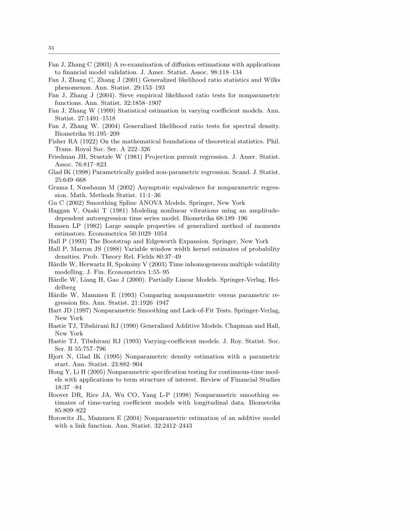
34
Fan J, Zhang C (2003) A re-examination of diffusion estimations with applicationsto financial model validation. J. Amer. Statist. Assoc. 98:118–134
Fan J, Zhang C, Zhang J (2001) Generalized likelihood ratio statistics and Wilksphenomenon. Ann. Statist. 29:153–193
Fan J, Zhang J (2004). Sieve empirical likelihood ratio tests for nonparametricfunctions. Ann. Statist. 32:1858–1907
Fan J, Zhang W (1999) Statistical estimation in varying coefficient models. Ann.Statist. 27:1491–1518
Fan J, Zhang W. (2004) Generalized likelihood ratio tests for spectral density.Biometrika 91:195–209
Fisher RA (1922) On the mathematical foundations of theoretical statistics. Phil.Trans. Royal Soc. Ser. A 222–326
Friedman JH, Stuetzle W (1981) Projection pursuit regression. J. Amer. Statist.Assoc. 76:817–823
Glad IK (1998) Parametrically guided non-parametric regression. Scand. J. Statist.25:649–668
Grama I, Nussbaum M (2002) Asymptotic equivalence for nonparametric regres-sion. Math. Methods Statist. 11:1–36
Gu C (2002) Smoothing Spline ANOVA Models. Springer, New YorkHaggan V, Ozaki T (1981) Modeling nonlinear vibrations using an amplitude-
dependent autoregression time series model. Biometrika 68:189–196Hansen LP (1982) Large sample properties of generalized method of moments
estimators. Econometrica 50:1029–1054Hall P (1993) The Bootstrap and Edgeworth Expansion. Springer, New YorkHall P, Marron JS (1988) Variable window width kernel estimates of probability
densities. Prob. Theory Rel. Fields 80:37–49Hardle W, Herwartz H, Spokoiny V (2003) Time inhomogeneous multiple volatility
modelling. J. Fin. Econometrics 1:55–95Hardle W, Liang H, Gao J (2000). Partially Linear Models. Springer-Verlag, Hei-
delbergHardle W, Mammen E (1993) Comparing nonparametric versus parametric re-
gression fits. Ann. Statist. 21:1926–1947Hart JD (1997) Nonparametric Smoothing and Lack-of-Fit Tests. Springer-Verlag,
New YorkHastie TJ, Tibshirani RJ (1990) Generalized Additive Models. Chapman and Hall,
New YorkHastie TJ, Tibshirani RJ (1993) Varying-coefficient models. J. Roy. Statist. Soc.
Ser. B 55:757–796Hjort N, Glad IK (1995) Nonparametric density estimation with a parametric
start. Ann. Statist. 23:882–904Hong Y, Li H (2005) Nonparametric specification testing for continuous-time mod-
els with applications to term structure of interest. Review of Financial Studies18:37 –84
Hoover DR, Rice JA, Wu CO, Yang L-P (1998) Nonparametric smoothing es-timates of time-varing coefficient models with longitudinal data. Biometrika85:809–822
Horowitz JL, Mammen E (2004) Nonparametric estimation of an additive modelwith a link function. Ann. Statist. 32:2412–2443
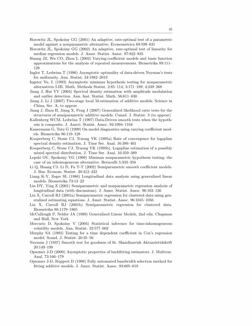
35
Horowitz JL, Spokoiny GG (2001) An adaptive, rate-optimal test of a parametricmodel against a nonparametric alternative. Econometrica 69:599–631
Horowitz JL, Spokoiny GG (2002) An adaptive, rate-optimal test of linearity formedian regression models. J. Amer. Statist. Assoc. 97:822–835
Huang JZ, Wu CO, Zhou L (2002) Varying-coefficient models and basis functionapproximations for the analysis of repeated measurements. Biometrika 89:111–128
Inglot T, Ledwina T (1996) Asymptotic optimality of data-driven Neyman’s testsfor uniformity. Ann. Statist. 24:1982–2019
Ingster Yu. I. (1993) Asymptotic minimax hypothesis testing for nonparametricalternatives I-III. Math. Methods Statist. 2:85–114; 3:171–189; 4:249–268
Jiang J, Hui YV (2004) Spectral density estimation with amplitude modulationand outlier detection. Ann. Inst. Statist. Math. 56:611–630
Jiang J, Li J (2007) Two-stage local M-estimation of additive models. Science inChina, Ser. A, to appear
Jiang J, Zhou H, Jiang X, Peng J (2007) Generalized likelihood ratio tests for thestructures of semiparametric additive models. Canad. J. Statist. 3 (to appear)
Kallenberg WCM, Ledwina T (1997) Data-Driven smooth tests when the hypoth-esis is composite. J. Ameri. Statist. Assoc. 92:1094–1104
Kauermann G, Tutz G (1999) On model diagnostics using varying coefficient mod-els. Biometrika 86:119–128
Kooperberg C, Stone CJ, Truong YK (1995a) Rate of convergence for logsplinespectral density estimation. J. Time Ser. Anal. 16:389–401
Kooperberg C, Stone CJ, Truong YK (1995b). Logspline estimation of a possiblymixed spectral distribution. J. Time Ser. Anal. 16:359–389
Lepski OV, Spokoiny VG (1999) Minimax nonparametric hypothesis testing: thecase of an inhomogeneous alternative. Bernoulli 5:333–358
Li Q, Huang CJ, Li D, Fu T-T (2002) Semiparametric smooth coefficient models.J. Bus. Econom. Statist. 20:412–422
Liang K-Y, Zeger SL (1986) Longitudinal data analysis using generalized linearmodels. Biometrika 73:13–22
Lin DY, Ying Z (2001) Semiparametric and nonparametric regression analysis oflongitudinal data (with discussions). J. Amer. Statist. Assoc. 96:103–126
Lin X, Carroll RJ (2001a) Semiparametric regression for clustered data using gen-eralized estimating equations. J. Amer. Statist. Assoc. 96:1045–1056
Lin X, Carroll RJ (2001b) Semiparametric regression for clustered data.Biometrika 88:1179–1865
McCullough P, Nelder JA (1989) Generalized Linear Models, 2nd edn. Chapmanand Hall, New York
Mercurio D, Spokoiny V (2004) Statistical inference for time-inhomogeneousvolatility models. Ann. Statist. 32:577–602
Murphy SA (1993) Testing for a time dependent coefficient in Cox’s regressionmodel. Scand. J. Statist. 20:35–50
Neyman J (1937) Smooth test for goodness of fit. Skandinavisk Aktuarietidskrift20:149–199
Opsomer J-D (2000) Asymptotic properties of backfitting estimators. J. Multivar.Anal. 73:166–179
Opsomer J-D, Ruppert D (1998) Fully automated bandwidth selection method forfitting additive models. J. Amer. Statist. Assoc. 93:605–619
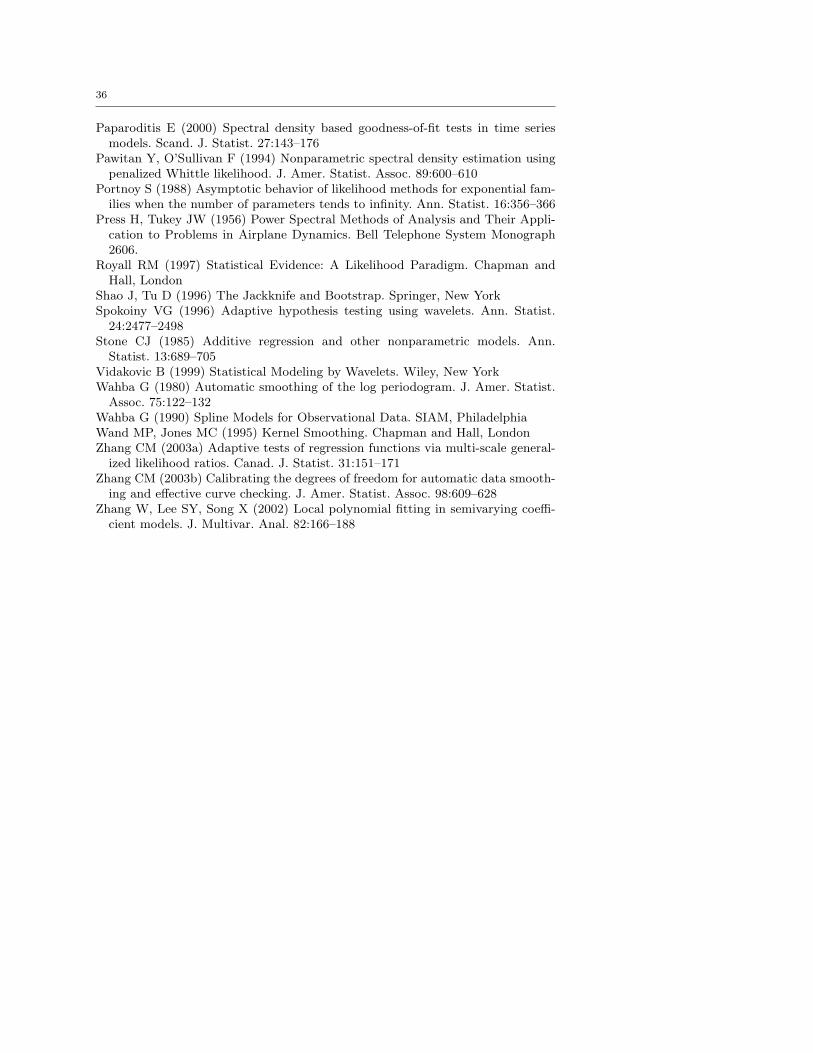
36
Paparoditis E (2000) Spectral density based goodness-of-fit tests in time seriesmodels. Scand. J. Statist. 27:143–176
Pawitan Y, O’Sullivan F (1994) Nonparametric spectral density estimation usingpenalized Whittle likelihood. J. Amer. Statist. Assoc. 89:600–610
Portnoy S (1988) Asymptotic behavior of likelihood methods for exponential fam-ilies when the number of parameters tends to infinity. Ann. Statist. 16:356–366
Press H, Tukey JW (1956) Power Spectral Methods of Analysis and Their Appli-cation to Problems in Airplane Dynamics. Bell Telephone System Monograph2606.
Royall RM (1997) Statistical Evidence: A Likelihood Paradigm. Chapman andHall, London
Shao J, Tu D (1996) The Jackknife and Bootstrap. Springer, New YorkSpokoiny VG (1996) Adaptive hypothesis testing using wavelets. Ann. Statist.
24:2477–2498Stone CJ (1985) Additive regression and other nonparametric models. Ann.
Statist. 13:689–705Vidakovic B (1999) Statistical Modeling by Wavelets. Wiley, New YorkWahba G (1980) Automatic smoothing of the log periodogram. J. Amer. Statist.
Assoc. 75:122–132Wahba G (1990) Spline Models for Observational Data. SIAM, PhiladelphiaWand MP, Jones MC (1995) Kernel Smoothing. Chapman and Hall, LondonZhang CM (2003a) Adaptive tests of regression functions via multi-scale general-
ized likelihood ratios. Canad. J. Statist. 31:151–171Zhang CM (2003b) Calibrating the degrees of freedom for automatic data smooth-
ing and effective curve checking. J. Amer. Statist. Assoc. 98:609–628Zhang W, Lee SY, Song X (2002) Local polynomial fitting in semivarying coeffi-
cient models. J. Multivar. Anal. 82:166–188