Supply Chain Network Design under Uncertainty with...

Noname manuscript No.(will be inserted by the editor)

Supply Chain Network Design under Uncertainty withEvidence Theory

Received: date / Accepted: date

Abstract In this paper, we present a new approach to design a multi-criteriasupply chain network (SCN) under uncertainty. Demands, supplies, produc-tion costs, transportation costs, opening costs are all considered as uncertainparameters. We propose an approach based on evidence theory (ET), ana-lytic hierarchy process (AHP) and two-stage stochastic programming (TSSP).First, we integrate ET and AHP in order to include several criteria (social, eco-nomical, and environmental) and the uncertain experts decisions for selectingthe best set of facilities. Second, we combine evidential data mining and TSSPapproach: (i) to design the SCN, (ii) to take into account the uncertainty ofsupply chain parameters, and (iii) to reduce scenarios number by retainingonly the significant ones. Finally, we illustrate the model with computationalstudy to highlight the practicality and the efficiency of the proposed method.

Keywords Supply chain design · Two-stage stochastic programming ·Evidence theory · Evidential data mining · BF-AHP

1 Introduction

The most challenging strategic issues that face business organizations todayare in the area of Supply Chain (SC). SC is a network of suppliers, factories,

Ahmed SametDepartment of Computing, Oxford Brookes University Wheatley Campus, Wheatley, Oxford(United Kingdom).E-mail: [email protected]

Yamine BouzembrakRIKILT Wageningen UR, Akkermaalsbos 2, 6708 WB Wageningen, The NetherlandsE-mail: [email protected]

Eric LefevreUniv. Lille Nord de France UArtois, EA 3926 LGI2A, F-62400, Bethune, FranceE-mail: [email protected]

2

warehouses, and distribution centers through which raw materials are pro-cured, transformed, and delivered to customers. The success of a SC dependson the most basic decision of SC management, which influences all other deci-sion levels. The topic of designing a SC is called supply chain network design(SCND). According to Chopra and Meindl [10], SCND problem comprises thedecisions regarding the number and location of production facilities, the ca-pacity of each facility, the assignment of each market region to one or morelocations, and supplier selection for sub-assemblies, components and materi-als. Extensive reviews surveying various issues in this area are available, forexample, in [19]. Indeed, building a sustainable supply chain nowadays hasbecome the ultimate objective of intelligent organizations, where the goal isnot only to minimize common costs, but also to integrate multi-criteria in theSCND and to reduce vulnerability due to uncertainty, by reducing possiblesources of losses [19,30,35].In this paper, we deal with the design of a multi-criteria SCN under uncertainenvironment in order to satisfy customers and to respect environmental, social,and economical requirements. We consider a multi-criteria, multi-level, singleproduct, uncertain SC parameters and single period SCND problem. The net-work has three levels: suppliers, production plants and customers. We proposea new approach based on evidence theory (ET), analytic hierarchy process(AHP) and two-stage stochastic programming (TSSP) to design a SCN underuncertainty. In this work, our most significant contributions are the follow-ing:(i) we integrate experts decisions uncertainty, environmental, social andeconomical aspects in the SCND problem using the BF-AHP method, (ii) weapply the ET, which is a strong formalism in modelling uncertainties, to definethe most relevant scenarios that can be used in the TSSP model. The set ofscenarios are mined from an expert opinion database with evidential data min-ing, (iii) we conduct a comprehensive set of numerical studies. Consequently,we reach some useful managerial insights.The rest of the paper is organized as follows. In section 2, we detail the litera-ture review. In section 3, the basics of ET are highlighted from the transferablebelief model interpretation [41]. In section 4, the new based belief SCND ap-proach is detailed. Section 5 includes application of the proposed model andoffers an analysis of the computational results. Finally, conclusions are drawnand perspectives are discussed in section 6.

2 Literature review

The business environment under which a SCN operates is unknown and criti-cal parameters such as customer demands, costs, quantities, and capacities areuncertain. The importance of uncertainty in SCND has encouraged researchersto handle stochastic parameters in SC problems [9,20,49]. Various modellingapproaches have been developed to deal with this complex problems, such asprobability theory, fuzzy sets theory [51], possibility theory [7,50], and theevidence theory [37].

Supply Chain Network Design under Uncertainty with Evidence Theory 3

In the area of stochastic SCND problems, scenario-based approaches such asTSSP result in more models [2,4,35,42,45,46]. Generally, in these studies, thefirst stage decisions belong to the strategic decision level, and second stage de-cisions are tactical and operational decisions are made. For instance, MirHas-sani et al. [24] presented a TSSP model to design a SCN with uncertain demandscenarios. The first stage decisions concern the location of plants and distribu-tion centers and the setting of their capacity levels. The second stage decisionsconcern the optimization of production and distribution quantities. Santoso etal. [35] proposed a TSSP for a multi-product SCND problem including suppli-ers, processing facilities, and warehouses. They also proposed an algorithm forsolving the problem and they used it for two realistic SCD problems. Azaronet al. [4] developed a multi-objective stochastic programming approach forSCD under uncertainty. They considered numerous uncertain parameters suchas: demands, supplies, processing, transportation, and capacity modificationcosts. The common points of these proposed approaches are: (i) minimizingcost or maximizing profit as a single objective is often the optimization focus.Literature surveys conducted by Seuring et al. [36] and Benjaafar et al. [5]have identified a growing need for developing quantitative models, methodsand approaches in sustainable SCND, (ii) in most multi-objective SCND ap-proaches, only demand is considered as the uncertainty source [16], (iii) in mostSCND problems under uncertainty only a few scenarios can be considered inthe optimization process due to the complexity of the problem. Although inmost practical situations, the number of possible scenarios is large. Accordingto [19] an importance based sampling approach must be developed to ensurethat all important plausible facets are covered in the small sample of scenariosselected.In literature, existing analytic hierarchy process approaches are applied tofacilitate location problems, where logistic actors are not considered in theselection criteria [3,44]. Tuzkaya et al. [43] included qualitative and quantita-tive criteria (benefits, opportunities, costs and risks), to assess and to selectundesirable facility locations. Kinra and Kotzab [18] suggested a simple AHPmodel to include constraints such as government regulations, policy, infrastruc-tural and political conditions, to find the best location of an industrial park.Few papers integrated ET in SC problems one of them is Wu and Barnes [48],which used the ET for formulating criteria to use in partner selection decision-making in agile supply chains. Wu [48] proposed a supplier selection in a fuzzygroup setting involving decisions balancing a number of conflicting criteria andopinions from different experts. In addition, only a few works got interested inintegrating data mining tools in the SC problems [8,26] despite their variousapplications [22]. Data mining techniques can be used to improve strategic andoperational planning activities [25]. However, SC literature lacks works thatintegrate imperfect data mining, which is an appropriate tool in case of treat-ing uncertain and imprecise data. More especially, no evidential data miningapproach has been applied to SCND problems.

4

3 The Evidence Theory

The ET (also called Belief Function Theory (BFT))1 was initiated by thework of Dempster [11] on upper and lower probabilities. The development ofthe theory formalism is owed to Shafer [37]. Shafer has shown the benefits ofET to model uncertain knowledge. In addition, it allows knowledge combina-tion obtained through various sources and it offers more flexibility than theprobabilistic framework does. Shafer’s book [37] has been followed by a largeliterature on interpretation, application, and computation [15,41]. For exam-ple, Smets [39,41] introduced a non probabilistic interpretation of ET calledTransferable Belief Model (TBM). In the remainder, we build our contributionbased on the Transferable Belief Model (TBM).

The Basic Belief Assignment (BBA) m is a function defined on each sub-space of the set of disjunctions of 2Θ and taking values in [0, 1]. Θ is theof all possible exclusive and exhaustive answers (hypothesis) for the treatedquestion and is called frame of discernment. It does not only represent all theconfidence granted to each possible response for the treated question but alsothe ignorance and the lack of certitude. A BBA m is modelled as follows:∑

A⊆Θm(A) = 1

m(∅) ≥ 0.(1)

Each hypothesis A having a belief value greater than 0 is called a focalelement. m(∅) is called the conflictual mass. A BBA is called normal wheneverthe emptyset is not a focal element and this corresponds to a closed worldassumption [38], otherwise it is said subnormal and it corresponds to an openworld assumption [41]. The closed world assumption is the assumption thatwhat is not known to be true must be false. The Open World Assumptionis the opposite. For more details, an example of BBA modelling is shown inAnnex A (Example 3).

When several information, modelled by BBAs, are induced from differentexperts, a fusion process is required. The ET proposes several operators ofcombination. One of the most used is the conjunctive rule of combination.This combination operator is used when sources (i.e. experts) are distinct andreliable. For two sources S1 and S2 having respectively m1 and m2 as BBAs,the conjunctive rule of combination is written as follows:

mΘ∩© = mΘ

1 ∩©mΘ2 . (2)

For an event A 6= ∅, mΘ∩© can be written as follows:

mΘ∩©(A) =

∑B∩C=Am

Θ1 (B) ·mΘ

2 (C) ∀A ⊆ ΘmΘ∩©(∅) ≥ 0.

(3)

1 In this paper we conjugate the use of the two designations of the theory. The belief func-tion theory designation is associated to the AHP method whereas ET is linked to evidentialdata mining.


where mΘ∩©(∅) corresponds to the conflict mass and highlights the degree of

contradiction between the combined sources (for further details the reader canrefer to Annex A, Example 4).

Decision functions allow the determination of the most suitable hypothesisfrom a BBA for the treated problem. In the TBM model, the pignistic level(i.e., decision level) allows to make decision from classical probabilities. Thepignistic probability [40], denoted BetP , was introduced by Smets [40] withinits TBM model. Not only does it makes probability transformation but italso takes into consideration the composite nature of focal elements. Formally,BetP is defined as follows:

BetP (Hn) =∑A⊆Θ

|Hn ∩A||A|

· m(A)

1−m(∅)∀Hn ∈ Θ. (4)

An example of pignistic probability use is provided in Example 5 in Annex A.In the following, we introduce the TSSP formulation to design a SCN

answering a real-world problem.

4 Solution approach

This section presents a real-world SCND problem. The potential design of asupply chain being considered by a textile company in France (Fig. 1) is com-posed of suppliers, production centres, and customers. Several criteria shouldbe integrated into the model, such as the total SC cost, jobless level, the qual-ity of the location and the environmental aspect. These criteria may affectthe selection of the facility locations, which is important for making an op-timal decision. The company is only interested in the SCND problem fromthe strategic point of view and model it as a multi-level, single-product andsingle-period problem. Accordingly, the modelling assumptions are as follows:- production costs [35], transportation costs [4], demands [29] and suppliedquantities [35] are uncertain parameters.- products are aggregated into a single product shipped through the SC net-work in a unique long-term period.

In the following, we detail the steps of our approach. This approach, asillustrated in Fig. 2, has four steps. The first step consists in storing the ex-perts’ preferences over a set of criteria in order to process them with BF-AHP.In fact, the second step is related to the best locations selection i.e., wherefacilities can be set-up respecting all criteria: environmental, social, and eco-nomical criteria. The BF-AHP method [6,12,13], that provides a convenientframework for dealing with uncertain data given by experts, is then used toselect the best alternative. As highlighted in [14], classical AHP method isoften criticized for its use of an unbalanced scale of estimations and its in-ability to adequately handle uncertainty and imprecision associated with themapping of the decision maker’s perception to a crisp number. In addition,

6

Fig. 1 Supply Chain Network

BF-AHP tolerates that an expert may be uncertain about his level of pref-erence due to incomplete information or knowledge, inherent complexity anduncertainty within the decision environment. Therefore, BF-AHP is an inter-esting approach to tackle uncertainty and imprecision within the pair-wisecomparison process, in particular, when the decision maker’s judgements arerepresented as a qualitative assessment. Once the best facilities are located,in the third step, experts are questioned over the optimal SCN configuration(called also scenarios) to meet customer demand minimizing the sum of costs.To select a subset of scenarios from a large set given by experts, for solvingthe TSSP model, the evidential data mining tools are used. Evidential datamining is very suited to handle large uncertain data and to associate a supportvalue (degree of frequency of an item within the database) to each selectedscenario. So, the last step combines ET and the TSSP model. These steps willbe detailed in the following subsections.

4.1 Belief Function AHP

The introduction of the BFT to the AHP method has brought flexibility in datatreatment. Indeed, imprecision and uncertainty are handled in the decision-making problem. The first step of this method consists in the identification ofthe set of criteria Ω and alternatives Θ. The expert can not only express hispreferences on the selected criteria but he can also do it on a set of them. Oncethe sets of criteria and alternatives are defined, the expert tries to specify hispreferences in order to obtain the criterion weights and the alternative scores interms of each criterion. Interested readers may refer to [13,14] for more detailof pair-wise comparisons and to preference elicitation. At the alternative level,unlike the criterion level, the expert tries to express his preferences over thesets of alternatives regarding each criterion. Accordingly, and to better imitatethe expert reasoning, we indicate that to define the influences of the criteriaon the evaluation of alternatives; we might use conditional belief that could


1 Expert evaluation 3Experts scenar-ios evaluation

4Stochastic Pro-

gramming2 BF-AHP

Uncertain AHP Com-parison Matrix

Uncertain SC parame-ters scenarios

Set of facilities

SC configuration

Fig. 2 Approach steps

be written as follows:

mΘ[cj ](Ak) = ωk, ∀Ak ⊂ 2Θ and cj ∈ Ω (5)

where Ak represents a subset of 2Θ, ωk is the eigen value of the kth sets ofalternatives regarding the criterion cj . m

Θ[cj ](Ak) means that we know thebelief about Ak regarding cj . The BF-AHP aims through this step to combinethe obtained conditional belief with the importance of their respective criteriato measure their contribution. Since the group of criteria and alternative thatrespectively belong to the frame of discernment Ω and Θ are different, theextension for constructed BBA is needed. At criterion level, the BBA mΩ isextended to Θ×Ω with the use of Equation (21)2. On the other hand, at alter-native level, the ballooning extension [28] is applied with the use of Equation(23)3. The ballooning extension consists at expressing a BBA, initially de-fined in the frame of discernment Θ, in a higher set Θ ×Ω. Finally, we mightcombine the obtained BBA with the importance of their respective criteriato measure their contribution. To that purpose, we will apply the conjunctiverule of combination so that:

mΘ×Ω = [ ∩©j=1,··· ,mmΘ[cj ]

⇑Θ×Ω ] ∩©mΩ↑Θ×Ω (6)

where mΩ↑Θ×Ω is the vacuous extension of mΩ which reflects the impor-tance of criteria. In order to make a decision, a marginalization4 is operatedon the resulting BBA over Θ with Equation (22). The decision is made over

2 Details about vacuous extension of Equation (21) are provided in the appendix.3 Details about operation in product space in belief function theory are provided in the

appendix.4 Details about marginalization of Equation (22) are provided in the appendix.

8

a set of probabilities found with the application of the pignistic probability(Equation (4)).

4.2 Evidential data mining and stochastic programming

In this step, we address the problem of reducing the number of scenarios inTSSP. The location of the facilities already computed with BF-AHP, we aimnow at finding the best scenarios (i.e., the best configuration). To do so, weaccess the opinion of several experts over set of parameters such as: the quan-tity (pieces), the transport unitary cost, the production unitary cost and thedemand. To handle these imprecise data (opinions), an uncertain data min-ing approach (or commonly called uncertain pattern mining approach) is re-quired. To deal with this problem, we propose the Expert Decision ConsensusApproach (EDeCA) based on evidential data mining [17,34], which reducesthe dimensions of the original scenarios set to a smaller set of scenarios. Thechoice of evidential data mining is motivated by its ability to model expert’sopinions even if they suffer from imprecision and uncertainty [21]. In addition,evidential data mining provides a generalizing framework for binary and otherimperfect data mining toolboxes [33]. Then, the stochastic program is solvedwith the smaller set of scenarios in order to obtain a representative solutionin reasonable time. In this subsection, we recall some basics of evidential datamining.

An evidential database is a database in which expert opinions are ex-pressed with basic belief assignment functions. Let us consider the set of nexperts E = E1, · · · , En. Each expert Ej gives his opinion with regards toa parameter (e.g the cost) i ∈ I that takes its value from the set Θi. Theset Θi = ω1

i , · · · , ωki is all possible choices (k ∈ [1, 2|Θi|]) that any expertmay pick for the parameter i. For an expert Ej and a parameter i, a BBA

mΘij : 2Θi −→ [0, 1] is modelled as follows:

∑ωki ⊆Θi

mΘij (ωki ) = 1

mΘij (∅) = 0.

(7)

The constructed evidential database that summarizes expert opinions isdenoted EDB. A focal element is commonly called an item. An itemset is a setof focal elements belonging to different parameters. In this work, an itemsethaving a size I (itemset containing items from each parameter) represents afeasible scenario.

Example 1 Table 1 shows an example of two experts having their opinionscaptured in an evidential database. The cost parameter takes its values withinthe frame of discernment Θ1 = High1, Low1 whereas the quantity parame-ter are within Θ2 = High2, Low2. mΘi

j (ωki ) highlights how confident the

expert j is that the parameter should be ωki .


Table 1 Supply chain parameter’s evidential database EDB

Expert Cost Quantity

E1 mΘ11 (High1) = 0.7 mΘ2

1 (High2) = 0.4

mΘ11 (Θ1) = 0.3 mΘ2

1 (Low2) = 0.2

mΘ21 (Θ2) = 0.4

E2 mΘ12 (Low1) = 0.3 mΘ2

2 (High2) = 1

mΘ12 (Θ1) = 0.7

The first row of the database means the expert E1 thinks that the costshould have a high value but he remains confused (mΘ1

1 (Θ1) > 0). Expert E2

is sure that the quantity should remain high (i.e, mΘ22 (High2) = 1). High1

is an item whereas High1 × Low2 is a scenario.

Once the supply chain parameter’s evidential database is constructed, themain task is to mine interesting scenarios. As it is the case for the other variantof data mining, the aim is to retrieve items and itemsets that have a degreeof presence (aka support) within the database greater than or equal to a fixedthreshold. In our problem, it means that we are aiming at retrieving valuableinformation supported by the majority of experts. In this part, we introducea new measure that we denote as the precise measure. This measure computesthe pertinence of all scenarios. For an item ωki , the precise measure is computedas follows:

Pr : 2Θ → [0, 1] (8)

Pr(ωki ) =∑ω⊆Θi

∣∣ωki ∩ ω∣∣|ω|

×m(ω) ∀ωki ∈ 2Θi . (9)

As illustrated above, the Pr(.) is a measure that computes the probabilityof presence of an item in a single BBA. The Pr is also assimilated to thepignistic probability in case of ωki ∈ Θi. For an itemset X =

∏i∈[1...I]

ωki and

satisfying the constraint⋂ωki

i∈I,k∈2|Θi|= ∅, its support (i.e., pertinence) for a

single expert Ej is computed with the precise measure as follows:

PrEj (X) =∏ωki ∈X

Pr(ωki ). (10)

Finally, the support of X in the entire database is deduced as follows:

PrEDB(X) =1

n

n∑j=1

PrEj (X). (11)

10

Example 2 Let us consider the Table 1. The precise measure of the scenariosX1 = Highc, Lowq and X2 = Highc, Highq is computed as follows:

PrEDB(X1) =PrE1(X1) + PrE2(X1)

2=

0.85× 0.4 + 0

2= 0.17

PrEDB(X2) =PrE1

(X2) + PrE2(X2)

2=

0.85× 0.6 + 0.35× 1

2= 0.43

The precise measure aims at estimating the support of each itemset. Inour problem, an itemset is assimilated to a scenario. The more the supportgrows for a scenario, the more priority it gains. Thus, with such use of support,we can retain opinions supported by the majority of experts. The scenarioshaving the highest precise value (i.e., support) gather somehow the consensusof studied experts. Therefore, the approach of extracting pertinent scenarioswith the precise measure is denoted as Expert Decision Consensus Approach(EDeCA). In addition, the precise support provides very precise estimationof the support comparatively to the other state-of-the-art alternative whichis the belief support [17]. As demonstrated recently in [31,34], the belief sup-port provides a pessimistic estimation of the support and therefore do notoutperform the precise support.

In pattern mining the definition of support is related to a threshold calledminsup [1]. Let us assume a threshold minsup and a scenario X, X is con-sidered as frequent as long as PrEDB(X) ≥ minsup. The threshold limits thenumber of retained scenarios. Only scenarios with a support greater or equalto minsup are retained in the set of frequent scenarios FS. The threshold isgenerally fixed by the expert. However, it still can be automatically computedto select only pertinent scenarios [27]. In Example 2, for a minsup fixed to0.4, X2 is considered as a frequent scenario.

Proposition 1 Let us consider the database EDB of n experts expressing theiropinions over I parameters. Let us consider two scenarios X1 and X2. X1 hasmore priority than X2 if and only if PrEDB(X1) > PrEDB(X2).

Despite, the frequency threshold constraint, the number of frequent sce-narios could still be to great to be evaluated. Therefore, several approachesfor selecting only the top-k best scenarios were provided [47]. A top-k miningapproach consists in retaining only the k frequent scenarios with the high-est utility. In this work, we fix k parameter proportionally to the size of thedatabase such as k = dn∗5100 e (five percent of the database). Therefore, thenumber of retrieved pertinent scenario do never exceed 5% of the databasesize. For the utility function, it is derived from Proposition 1 where only thosefrequent scenarios maximizing the support are retained.

Using the set of facility locations obtained solving the belief AHP and thereduced set of scenarios along with their precise measures obtained by solvingEDeCA approach, we design the supply chain network of the problem solvingthe TSSP presented in Equations (12) to (19).

We consider a network G = (NO,AC) (Fig. 1), where NO is the set ofnodes and AC is the set of arcs. The SCN consists of the set of suppliers


S, the set of processing facilities Θ and the set of customers C. R is theset of scenarios. The SC configuration decisions consist in deciding which ofthe manufacturing facilities to open and the quantity of products transportedthrough the SCN. We associate a binary variable yi to the location decisions,yi = 1, if a manufacturing facility i is built, and 0 otherwise. We let xij denotethe flow of product from a node i to a node j of the network where (ij) ∈ AC.

We model the SC as two-stage stochastic program (see [2,4,35,45,46]).For reasons of simplicity, we denote the set of feasible solution of first-stagedecisions yi by Y . The uncertain parameter in this formulation is: productioncosts, transportation costs, opening costs, demands and supplies. The firststage consists in determining the configuration decisions y, and the secondstage consists of the quantities of goods to transport throughout the supplychain network in an optimal way. Note that ξ represents the random vectorcorresponding to the uncertain parameters. The design objective is to minimizethe sum of investment costs and expected future variable costs. The strategicSCN that we intend to establish, should answer the following questions underuncertain environment: (i) how many manufacturing plants should be installed(ii) where the new sites should be located (iii) how much goods the productionplant should handle (iv) what products quantities to transport throughoutthe supply chain network. The minimization of the sum of investment can bewritten as follows:

Min∑i∈Θ

oci · yi +∑s∈R

ρsQ(y, ξs) (12)

subject to:

y ∈ Y ⊆ 0, 1n (13)

with Q(y,ξs) being the solution of the following second stage problem:

Min∑

i∈S,j∈Θ

µsβij · xsij +∑

j∈Θ,k∈C

µsβjk · xsjk +∑

i∈S,j∈Θ

fsj · xsij s ∈ R. (14)

subject to: ∑i∈S,j∈Θ

xsij ≤ Asi i ∈ S; s ∈ R. (15)

∑i∈S

xsij −∑k∈C

xsjk = 0 j ∈ Θ; s ∈ R. (16)

∑i∈S

xsij ≤ Fmaxj · yj j ∈ Θ; s ∈ R. (17)

∑j∈Θ

xsjk ≥ dsk k ∈ C, s ∈ R. (18)

xsij ≥ 0 i ∈ S, j ∈ Θ, s ∈ R. (19)

12

xsjk ≥ 0 j ∈ Θ, k ∈ C, s ∈ R. (20)

where oci denotes the opening cost for building facility i, and ρs is the proba-bility of each scenario. The first-stage consists of configuration decisions y, theobjective is to minimize investment costs and future operating costs (Equa-tion 12). The second-stage consists of optimal production and transportationof products through the SC based on the configuration and the realized un-certain scenario (Equation 14). fsj is the unit production cost of each productat facility j and µs presents unit transportation cost of each product and βijis the distance between i and j on arc (ij). Constraint (15) requires that thetotal flow of products from a supplier j, should be less than the supply Aj atthat node. Constraint (16) enforces the flow conservation of products acrosseach processing node j. Constraint (17) represents the capacity constraint whorequires that the total processing requirement of all products flowing into aprocessing node j should be smaller than the capacity Fmaxj of facility j if itis built (yj = 1). If facility j is not built (yj = 0) the constraint will force allflow variables xij = 0 for all i ∈ N . Constraint (18) requires that the totalflow of products sent to a customer j should exceed the demand dk of cus-tomer k. Finally, constraints (19) and (20) enforce the non-negativity of theflow variables.

5 Computational experiments

In this section, we present the results of the analysis. In order to evaluatethe model, we present an example of SC. The SCN consists of 4 possiblelocations for production center, 3 suppliers from whom goods are supplied,and 10 customers that the company serves. We propose an ET-TSSP modelin which we involve 100 experts’ scenarios and 4 criteria: investment costs,environmental risks, location, social aspect. The uncertain parameters are:the experts decisions in the selection of the best facility location set, customerdemand, transportation costs, production costs and supplied quantities. Onehundred scenarios are proposed by several experts for TSSP and all thesescenarios are reduced to 5 best scenarios using the evidential data miningtool. The TSSP problem was solved using ILOG CPLEX 12.0 solver. All theexperiments are conducted on a PC with Intel Core 2 Duo 2.19 GHz and 2 GBRAM. A comparison between the deterministic approach and the stochasticsolution is performed next.

5.1 Belief AHP results

Before running the TSSP model, the first step is to obtain a set of potentialfacility locations. As mentioned in section 4, the potential set of facilities needsto be computed using BF-AHP. To select the best facility locations, we reliedon four important criteria: Ω = investment costs (C1), environmental risks


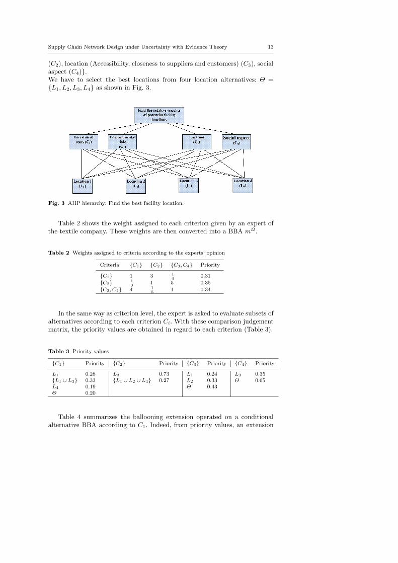
(C2), location (Accessibility, closeness to suppliers and customers) (C3), socialaspect (C4).We have to select the best locations from four location alternatives: Θ =L1, L2, L3, L4 as shown in Fig. 3.

Fig. 3 AHP hierarchy: Find the best facility location.

Table 2 shows the weight assigned to each criterion given by an expert ofthe textile company. These weights are then converted into a BBA mΩ .

Table 2 Weights assigned to criteria according to the experts’ opinion

Criteria C1 C2 C3, C4 Priority

C1 1 3 14

0.31

C2 13

1 5 0.35

C3, C4 4 15

1 0.34

In the same way as criterion level, the expert is asked to evaluate subsets ofalternatives according to each criterion Ci. With these comparison judgementmatrix, the priority values are obtained in regard to each criterion (Table 3).

Table 3 Priority values

C1 Priority C2 Priority C3 Priority C4 Priority

L1 0.28 L3 0.73 L1 0.24 L3 0.35L1 ∪ L3 0.33 L1 ∪ L2 ∪ L4 0.27 L2 0.33 Θ 0.65L4 0.19 Θ 0.43Θ 0.20

Table 4 summarizes the ballooning extension operated on a conditionalalternative BBA according to C1. Indeed, from priority values, an extension

14

is operated following Equation (23). This operation is repeated for the otherpriority values obtained according to criteria.

Table 4 Ballooning extension mΘ[C1]⇑Θ×Ω of conditional BBA mΘ[C1]

conditional bbm Ballooning extension Values

mΘ[C1](L1) (L1, C1), Θ × C2, C3, C4 0.28mΘ[C1](L2 ∪ L3) (L2, C1), (L3, C1), Θ × C2, C3, C4 0.33mΘ[C1](L4) (L4, C1), Θ × C2, C3, C4 0.19mΘ[C1](Θ) Θ ×Ω 0.20

The final results are shown in Table 5 in which the resulting BBA is de-tailed. This BBA is obtained, with Equation (6) after combining extendedconditional BBAs (mΩ [Ci]

⇑Θ×Ω) with criteria BBA (mΩ) which is previouslyextended to Θ ×Ω and marginalization on Θ (Equation (22)).

Table 5 The obtained BBA mΘ×Ω↓Θ and the confidence of location possibilities

L1 0.13L2 0.07L3 0.30L4 0.06L1, L3 0.04L2, L3 0.14L1, L2, L4 0.10Θ 0.09∅ 0.07

After the pignistic transformation, the results obtained from the compu-tation of the weights using the BF-AHP method for four criteria and fouralternatives are shown in Table 6. The priority weights of the four alterna-tives (L1, L2, L3, L4) are 0.22, 0.21, 0.45, 0.12 respectively. They imply thatthe third alternative (L3) and the first alternative (L1) are the best facilitylocations. These locations are then used in the second step to design the SCNusing TSSP.

Table 6 The final BBA mΘ and locations’ priority

Alternative priority

L1 0.22L2 0.21L3 0.45L4 0.12


5.2 EDeCA results

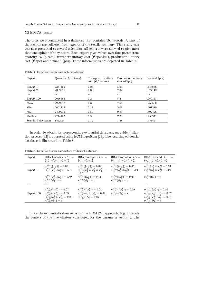
The tests were conducted in a database that contains 100 records. A part ofthe records are collected from experts of the textile company. This study casewas also presented to several scientists. All experts were allowed to give morethan one opinion if they desire. Each expert gives values over four parameters:quantity Ai (pieces), transport unitary cost (AC/pcs.km), production unitarycost (AC/pc) and demand (pcs). These informations are depicted in Table 7.

Table 7 Expert’s chosen parameters database

Expert Quantity Ai (pieces) Transport unitarycost (AC/pcs.km)

Production unitarycost (AC/pc)

Demand (pcs)

Expert 1 2381409 0.26 5.05 1148838Expert 2 2399271 0.33 7.04 1077142

· · · · · · · · · · · · · · ·Expert 100 2046663 0.2 5.2 1060153

Mean 2222917 0.3 7.64 1259580

Min 2002113 0.11 5.01 1001389

Max 2499212 0.50 9.89 1497426

Median 2214462 0.3 7.73 1250971

Standard deviation 147200 0.12 1.48 145745

In order to obtain its corresponding evidential database, an evidentializa-tion process [32] is operated using ECM algorithm [23]. The resulting evidentialdatabase is illustrated in Table 8.

Table 8 Expert’s chosen parameters evidential database

Expert BBA Quantity Θ1 =ω1

1 , ω21 , ω

31 , ω

41 , ω

51

BBA Transport Θ2 =ω1

2 , ω22 , ω

32

BBA Production Θ3 =ω1

3 , ω23 , ω

33 , ω

43 , ω

53

BBA Demand Θ4 =ω1

4 , ω24 , ω

34 , ω

44 , ω

54

mΘ11 (ω2

1) = 0.02 mΘ21 (ω3

2) = 0.021 mΘ31 (ω2

3) = 0.85 mΘ41 (ω1

4 ∪ ω54) = 0.94

Expert 1 mΘ11 (ω2

1 ∪ ω41) = 0.07 mΘ2

1 (ω12 ∪ ω2

2 ∪ ω32) =

0.82mΘ3

1 (ω13 ∪ ω2

3) = 0.04 mΘ41 (ω2

4 ∪ ω54) = 0.01

mΘ11 (ω3

1 ∪ ω41) = 0.89 mΘ2

1 (ω42) = 0.11 mΘ3

1 (ω33) = 0.05 mΘ4

1 (Θ4) = ε

mΘ11 (Θ1) = ε mΘ2

1 (Θ2) = ε mΘ31 (Θ3) = ε

· · · · · · · · · · · · · · ·

mΘ1100(ω3

1) = 0.07 mΘ2100(ω1

2) = 0.04 mΘ3100(ω1

3) = 0.99 mΘ4100(ω4

4) = 0.16

Expert 100 mΘ1100(ω5

1) = 0.03 mΘ2100(ω2

2 ∪ ω32) = 0.09 mΘ3

100(Θ3) = ε mΘ4100(ω1

4 ∪ ω44) = 0.07

mΘ1100(ω3

1 ∪ ω51) = 0.86 mΘ2

100(Θ2) = 0.87 mΘ4100(ω4

4 ∪ ω54) = 0.57

mΘ1100(Θ1) = ε mΘ4

100(Θ4) = ε

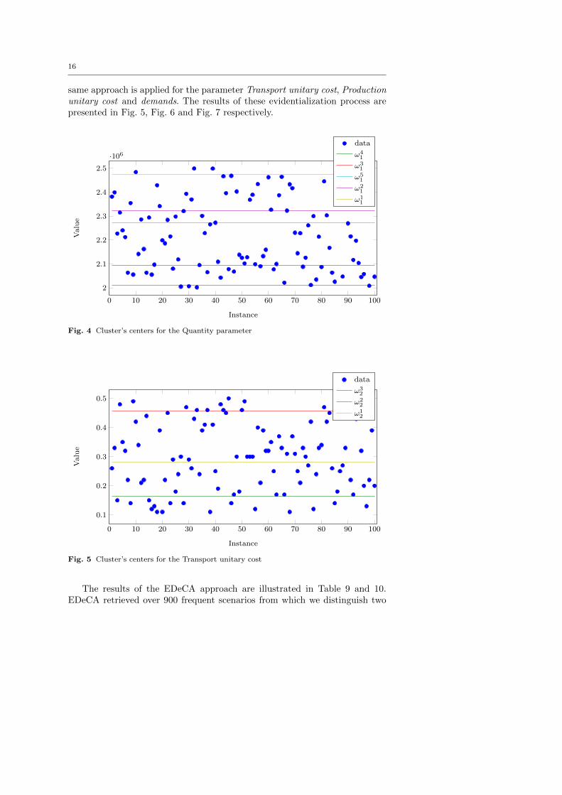
Since the evidentialization relies on the ECM [23] approach, Fig. 4 detailsthe centers of the five clusters considered for the parameter quantity. The

16

same approach is applied for the parameter Transport unitary cost, Productionunitary cost and demands. The results of these evidentialization process arepresented in Fig. 5, Fig. 6 and Fig. 7 respectively.

0 10 20 30 40 50 60 70 80 90 100

2

2.1

2.2

2.3

2.4

2.5

·106

Instance

Valu

e

data

ω41

ω31

ω51

ω21

ω11

Fig. 4 Cluster’s centers for the Quantity parameter

0 10 20 30 40 50 60 70 80 90 100

0.1

0.2

0.3

0.4

0.5

Instance

Valu

e

data

ω32

ω22

ω12

Fig. 5 Cluster’s centers for the Transport unitary cost

The results of the EDeCA approach are illustrated in Table 9 and 10.EDeCA retrieved over 900 frequent scenarios from which we distinguish two


0 10 20 30 40 50 60 70 80 90 100

5

6

7

8

9

10

Instance

Valu

e

data

ω33

ω43

ω53

ω13

ω23

Fig. 6 Cluster’s centers for the Production unitary cost

0 10 20 30 40 50 60 70 80 90 100

1

1.1

1.2

1.3

1.4

1.5

·106

Instance

Valu

e

data

ω54

ω44

ω34

ω24

ω14

Fig. 7 Cluster’s centers for the Demands

categories. The first category regroups over 500 imprecise scenarios which wedenote as the vague ones. Indeed, to each single parameter, the EDeCA ap-proach retains a vague focal element (disjunction of hypothesis). These kindsof scenario are important since it gives the decision maker an idea about thevalues that he must avoid and those he must consider. In our tests, we considerthe top-k best scenarios and they are shown in Table 9 where k is fixed to 5.So, these scenarios are then ranked by their pertinence. The second categoryregroups the precise frequent scenarios i.e., those constituted by simple focal

18

elements (singleton hypothesis). The precise scenarios point out which param-eter’s value the decider has to choose. The top-5 precise scenarios are shownin Table 10

Table 9 5 best vague scenarios

Scenario Pertinence

ω11 ∪ ω2

1 ∪ ω31 ∪ ω4

1, Θ2, ω13 ∪ ω2

3 ∪ ω33 ∪ ω4

3, Θ4 0.773ω1

1 ∪ ω21 ∪ ω3

1 ∪ ω41, Θ2, ω1

3 ∪ ω23 ∪ ω3

3 ∪ ω53, Θ4 0.712

ω11 ∪ ω3

1 ∪ ω41 ∪ ω5

1, Θ2, ω13 ∪ ω2

3 ∪ ω33 ∪ ω4

3, Θ4 0.709ω1

1 ∪ ω31 ∪ ω4

1 ∪ ω51, Θ2, ω1

3 ∪ ω23 ∪ ω3

3 ∪ ω53, Θ4 0.699

ω11 ∪ ω2

1 ∪ ω31 ∪ ω4

1, Θ2, ω13 ∪ ω2

3 ∪ ω43 ∪ ω5

3, Θ4 0.689

Table 10 5 best precise scenarios

Scenario Pertinence Probability of scenario

ω31 , ω

32 , ω

23 , ω

14 0.015 0.28

ω41 , ω

22 , ω

13 , ω

54 0.012 0.22

ω41 , ω

22 , ω

13 , ω

44 0.009 0.17

ω41 , ω

32 , ω

23 , ω

34 0.009 0.17

ω41 , ω

32 , ω

33 , ω

44 0.009 0.16

By comparing the pertinence in Table 9 and 10, we notice that the vaguescenarios present a better pertinence than the precise ones. This result was tobe expected due to the nature of the pertinence formula (Equation (11)) andits pignistic probability basics. The more the considered scenario is vague, themore pertinence it gathers. On the other hand, our EDeCA approach gives aclassification of both scenario categories. Even if the pertinence of the precisescenarios is low, EDeCA shows a ranked list of the best scenarios to rely on.

5.3 Two-stage stochastic model results

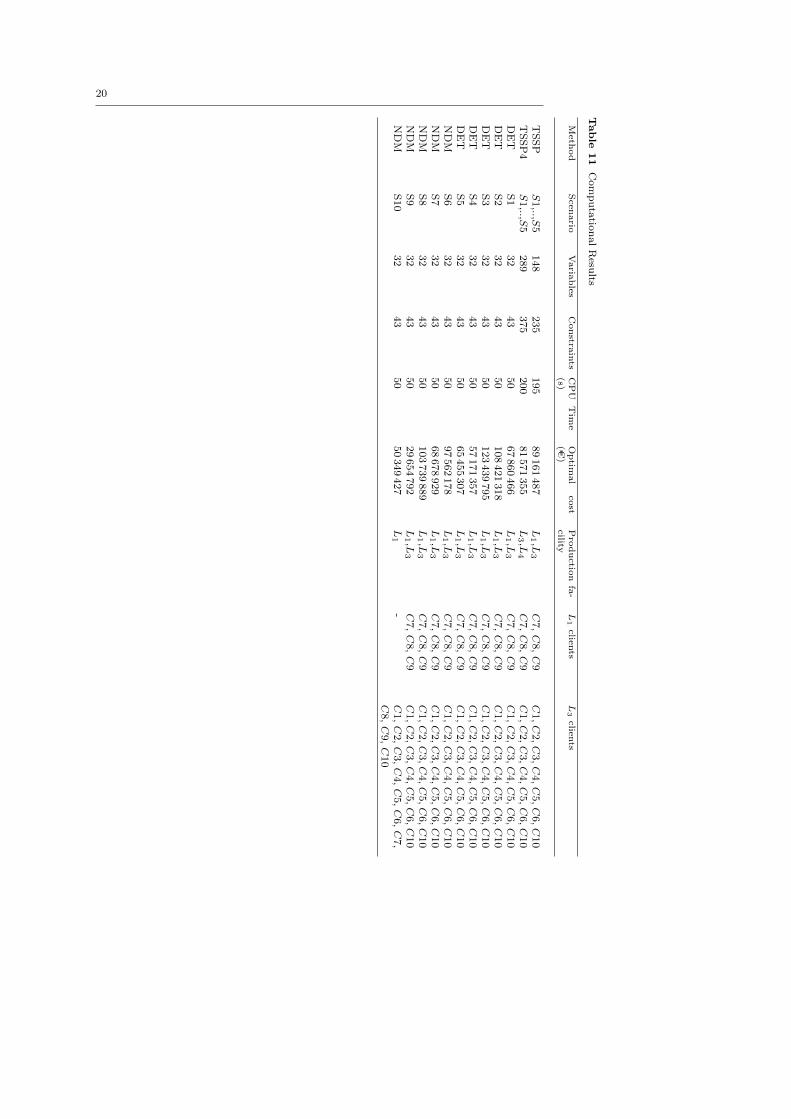
In this step, we study the configuration of the supply chain network. By usingthe set of facility locations and the reduced set of scenarios obtained in thepreview step we solve the mathematical model (12)-(19). The values for theSC uncertain parameters are the same as in Table 10. In order to generatea balanced network configuration between these various scenarios, we appliedstochastic programming with equal probabilities. Table 11 summarizes the re-sults of the TSSP model, deterministic (DET), and normal distribution model(NDM). TSSP solution is obtained solving the TSSP model considering the5 scenarios of EDeCA results and the best two facility locations L1 and L3.TSSP4 solution is obtained solving the TSSP model considering the 5 scenar-ios of EDeCA results and the four location alternatives: Θ = L1, L2, L3, L4.


A deterministic model is used to solve each scenario individually (S1,..,S5).Scenarios (S6,..,S10) are generated assuming that the uncertain parametersfit to normal distribution.

Table 11 reveals that, for this case, the TSSP model contains 148 variablesand 235 constraints. As we can see, for 5 scenarios the CPU Time is equal to195 seconds, and it can easily go up with the growing of scenario numbers andthe size of the supply chain. The SC configuration proposed is to open twoproduction plants L1 and L3. The affectation of customers to each productionfacility is depicted in Fig. 8. To satisfy customers demand the productionplant L1 should deliver products to 3 customers (C7, C8, C9) and L3 shouldsupply products to customers (C1, C2, C3, C4, C5, C6, C10). The solution ofTSSP4 is to open two production facilities L3 and L4. The production plant L3

delivers the products to four customers (C1, C2, C3, C5) and L4 supplies theother customers. The best facilities selected in this case are different than thefacilities obtained solving the BF-AHP, because only the economic aspect wasconsidered in the TSSP model. The solutions obtained using the TSSP modelare feasible only because of the high capacity of the suppliers and the non-consideration of the capacity constraints. Comparing the TSSP solution to thedeterministic ones the structure of the SCN is the same in the all scenarios.This can be explained by the low uncertainty of the SC parameters and thesmall size of the case study. The NDM model exhibits two different SCNs,for scenarios (S6,S7,S8,S9) the optimal solution is to open two facilities L1

and L3 and for scenario S10, the SC configuration proposed is to open oneproduction plant (L1).

Fig. 8 Customers affectation

6 Conclusions

In this paper, we introduce a multi-criteria SCND under uncertainty modelbased on the evidence theory. The main contribution of the model is the inte-gration of multi-criteria aspect and uncertainty of SC parameters in the designof SCN using the belief AHP and TSSP.The approach contains two steps, the aim of the first step is to select the best

20

Tab

le11

Com

pu

tatio

nal

Resu

lts

Meth

od

Scenario

Varia

bles

Constra

ints

CPU

Tim

e(s)

Optim

al

cost

(AC)

Pro

ductio

nfa-

cility

L1clie

nts

L3clie

nts

TS

SP

S1,..,S

5148

235

195

89

161

487

L1,L

3C

7,C

8,C

9C

1,C

2,C

3,C

4,C

5,C

6,C

10

TS

SP

4S

1,..,S

5289

375

200

81

571

355

L3,L

4C

7,C

8,C

9C

1,C

2,C

3,C

4,C

5,C

6,C

10

DE

TS

132

43

50

67

860

466

L1,L

3C

7,C

8,C

9C

1,C

2,C

3,C

4,C

5,C

6,C

10

DE

TS

232

43

50

108

421

318

L1,L

3C

7,C

8,C

9C

1,C

2,C

3,C

4,C

5,C

6,C

10

DE

TS

332

43

50

123

439

795

L1,L

3C

7,C

8,C

9C

1,C

2,C

3,C

4,C

5,C

6,C

10

DE

TS

432

43

50

57

171

357

L1,L

3C

7,C

8,C

9C

1,C

2,C

3,C

4,C

5,C

6,C

10

DE

TS

532

43

50

65

455

307

L1,L

3C

7,C

8,C

9C

1,C

2,C

3,C

4,C

5,C

6,C

10

ND

MS

632

43

50

97

562

178

L1,L

3C

7,C

8,C

9C

1,C

2,C

3,C

4,C

5,C

6,C

10

ND

MS

732

43

50

68

678

929

L1,L

3C

7,C

8,C

9C

1,C

2,C

3,C

4,C

5,C

6,C

10

ND

MS

832

43

50

103

739

889

L1,L

3C

7,C

8,C

9C

1,C

2,C

3,C

4,C

5,C

6,C

10

ND

MS

932

43

50

29

654

792

L1,L

3C

7,C

8,C

9C

1,C

2,C

3,C

4,C

5,C

6,C

10

ND

MS

10

32

43

50

50

349

427

L1

-C

1,C

2,C

3,C

4,C

5,C

6,C

7,

C8,C

9,C

10


locations where plants can be opened. We used the belief AHP method to in-tegrate uncertain information given by experts and to consider many criteriain the selection: environmental, social, and economical. In the second step, weconsider that all SC parameters of the model are uncertain: transportationcosts, production costs, customers demand and supplied quantities. So, weused the evidential data mining to select a subset of scenarios from a large setgiven by experts and TSSP to model the problem.Several possible future research avenues can be defined in this context. Forinstance, addressing uncertainty in the suppliers capacity, the production ca-pacity and the location of customers may be attractive direction for futureresearch. Also, testing the approach on large scale SCN is not addressed inthis paper. Therefore the evaluation of the model on large SCN and compar-ing its efficiency to other methods can be an interesting development in thisarea.

Acknowledgements

The authors would like to express their sincere gratitude to the reviewers fortheir constructive and helpful comments and suggestions which have been inhelp to improve the quality of this paper. The authors would like to thankProf. Alexandre Termier and Dr. Thomas Guyet at IRISA laboratory for theiradvices and their feedbacks.

A Examples on belief function operations described in Section 3

Example 3 Let us assume a company that plans to relocate its factory to optimize itsrevenues. The factory should be either set up in the downtown of a big city or in its suburbsfor supplying transport constraints i.e., Ω = Downtown, Suburb. Thus, three locationshave emerged and are discussed i.e., Θ = Paris, Lille, Berlin. Both Ω and Θ are framesof discernment. One expert has been questioned about the location problem and below ishis answer modelled with a BBA.

mΘ(Paris) = 0.5

mΘ(Lille) = 0.2

mΘ(Θ) = 0.3

mΘ(Θ) = 0.3 means that the expert has some doubts over the given location possibilities.This uncertainty is expressed by assigning a value to the frame of discernment Θ.

Example 4 Let us consider Θ = Paris, Lille, Berlin. Two experts have been questionedover the best possible location for the factory. Both opinions are highlighted in the followingBBAs:

mΘ1 (Paris) = 0.5

mΘ1 (Lille) = 0.2

mΘ1 (Θ) = 0.3

mΘ2 (Paris) = 0.4

mΘ2 (Berlin) = 0.4

mΘ2 (Θ) = 0.2

22

Thus, the result of the combination sum is equal to :

m ∩©(∅) = 0.36

m ∩©(Paris) = 0.42

m ∩©(Lille) = 0.04

m ∩©(Berlin) = 0.12

m ∩©(Θ) = 0.06

For example m ∩©(Paris) is computed as the sum of mΘ1 (Paris) × mΘ2 (Paris) +mΘ1 (Paris)×mΘ2 (Θ) +mΘ2 (Paris)×mΘ1 (Θ).

Example 5 Assuming the BBA obtained through the conjunctive rule of combination inExample 4. To make a final decision, it is possible to recover a set of probabilities from aBBA with the pignistic probability as follows:

BetP (Paris) = 0.69

BetP (Lille) = 0.09

BetP (Berlin) = 0.22

B Operation on the product space in belief function theory

Let U = X,Y, Z, . . . be a set of variables, each one has its frame of discernment. Let Xand Y be two disjoint subsets of U . Their frames are the product space of the frames of thevariables they include.

Given a BBA defined on X, its vacuous extension on X ×Y denoted mX↑X×Y is givenby:

mX↑X×Y (B) =

mX(A) if B = A× Y,A ⊂ X,0 otherwise.

(21)

Example 6 Let us assume the example depicted in Example 3. The BBA defined on Θ willbe defined in a finer frame Θ ×Ω using the vacuous extension as follows:

mΘ↑Θ×Ω(Paris,Downtown, Paris, Suburb) = 0.5

mΘ↑Θ×Ω(Lille,Downtown, Lille, Suburb) = 0.2

mΘ↑Θ×Ω(Θ ×Ω) = 0.3

A BBA defined on a product space X × Y may be marginalized on X by transferringeach mass mX×Y (B) from B ⊂ X × Y to its projection on X:

mX×Y ↓X(A) =∑

B⊂X×Y |Proj(B↓X)=A

mX×Y (B),∀A ⊂ X (22)

where Proj(B ↓ X) denotes the projection of B onto X.

Example 7 Let us assume the following BBA defined over Θ ×Ω:mΘ×Ω(Paris,Downtown, Paris, Suburb) = 0.5

mΘ×Ω(Lille,Downtown, Lille, Suburb) = 0.2

mΘ×Ω(Paris,Downtown) = 0.3

Marginalizing of mΘ×Ω on the coarser frame Θ gives the following mΘ×Ω↓Θ:mΘ×Ω↓Θ(Paris) = 0.5 + 0.3 = 0.8

mΘ×Ω↓Θ(Lille) = 0.2


Let mX [B] represent the beliefs X conditionally on B a subset of Y , i.e., in a contextwhere B holds. The ballooning extension is defined as:

mX [B]⇑X×Y (A×B ∪X ×B) = mX [B](A), ∀A ⊂ X. (23)

Example 8 Let us consider Θ = Paris, Lille, Berlin, Ω = Downtown, Suburb and theconditional BBA mΘ[Downtown](Paris) = 0.6. Its corresponding BBA on Θ × Ω isobtained by taking into consideration Paris,Downtown and all the instances of Θ for thecomplement of Downtown.mΘ[Downtown]⇑Θ×Ω((Paris,Downtown), (Paris, Suburb), (Lille, Suburb),(Berlin, Suburb)) = mΘ[Downtown](Paris).

References

1. Agrawal, R., Srikant, R.: Fast algorithm for mining association rules. In Proceedingsof international conference on Very Large DataBases, VLDB, Santiago de Chile, Chilepp. 487–499 (1994)

2. Alonso-Ayuso, A., Escudero, L., Ortuo, M.: 13. Modeling Production Planning andScheduling under Uncertainty, chap. 13, pp. 217–252 (2005)

3. Aras, H., Erdogmus, S., Koc, E.: Multi-criteria selection for a wind observation stationlocation using Ananalytic Hierarchy Process. Renewable Energy 29(8), 1383 – 1392(2004)

4. Azaron, A., Brown, K., Tarim, S., Modarres, M.: A multi-objective stochastic pro-gramming approach for supply chain design considering risk. International Journal ofProduction Economics 116(1), 129 – 138 (2008)

5. Benjaafar, S., Li, Y., Daskin, M.: Carbon footprint and the management of supplychains: Insights from simple models. Automation Science and Engineering, IEEE Trans-actions on 10(1), 99–116 (2013)

6. Beynon, M., Curry, B., Morgan, P.: The Dempster–Shafer theory of evidence: an alter-native approach to multicriteria decision modelling. Omega 28(1), 37–50 (2000)

7. Bouzembrak, Y., Allaoui, H., Goncalves, G., Bouchriha, H., Baklouti, M.: A possibilisticlinear programming model for supply chain network design under uncertainty. IMAJournal of Management Mathematics 24(2), 209–229 (2013)

8. Chen, A., Liu, L., Chen, N., Xia, G.: Application of data mining in supply chain manage-ment. in Proceedings of the 3rd World Congress on Intelligent Control and Automation3, 1943–1947 vol.3 (2000)

9. Cheung, R.K.M., Powell, W.B.: Models and algorithms for distribution problems withuncertain demands. Transportation Science 30, 43–59 (1996)

10. Chopra, S., Meindl, P.: Supply chain management: strategy, planning, and operation.Pearson Prentice Hall (2007)

11. Dempster, A.: Upper and lower probabilities induced by multivalued mapping. AMS-38(1967)

12. Dezert, J., Tacnet, J.M., Batton-Hubert, M., Smarandache, F., et al.: Multi-criteriadecision making based on DSmT-AHP. BELIEF 2010: Workshop on the Theory ofBelief Functions, Brest, France (2010)

13. Ennaceur, A., Elouedi, Z., Lefevre, E.: Reasoning under uncertainty in the AHP methodusing the belief function theory. In Proceedings of 14th International Conference onInformation Processing and Management of Uncertainty in Knowledge-Based Systems,IPMU 2012, Catania, Italy 4, 373–382 (2012)

14. Ennaceur, A., Elouedi, Z., Lefevre, E.: Multi-criteria decision making method with beliefpreference relations. International Journal of Uncertainty, Fuzziness and Knowledge-Based Systems 22(4), 573–590 (2014)

15. Gardenfors, P.: Probabilistic reasoning and evidentiary value. In: Evidentiary Value:Philosophical, Judicial, and Psychological Aspects of a Theory: Essays Dedicated toSoren Hallden on His Sixtieth Birthday. C.W.K. Gleerups (1983)

16. Guilln, G., Mele, F., Bagajewicz, M., Espua, A., Puigjaner, L.: Multiobjective supplychain design under uncertainty. Chemical Engineering Science 60(6), 1535–1553 (2005)

24

17. Hewawasam, K.K.R., Premaratne, K., Shyu, M.L.: Rule mining and classification in asituation assessment application: A belief-theoretic approach for handling data imper-fections. Trans. Sys. Man Cyber. Part B 37(6), 1446–1459 (2007)

18. Kinra, A., Kotzab, H.: A macro-institutional perspective on supply chain environmentalcomplexity. International Journal of Production Economics 115(2), 283–295 (2008).Institutional Perspectives on Supply Chain Management

19. Klibi, W., Martel, A., Guitouni, A.: The design of robust value-creating supply chainnetworks: A critical review. European Journal of Operational Research 203(2), 283 –293 (2010)

20. Landeghem, H.V., Vanmaele, H.: Robust planning: a new paradigm for demand chainplanning. Journal of Operations Management 20(6), 769 – 783 (2002)

21. Lee, S.: Imprecise and uncertain information in databases: an evidential approach. InProceedings of Eighth International Conference on Data Engineering, Tempe, AZ pp.614–621 (1992)

22. Liao, S.H., Chu, P.H., Hsiao, P.Y.: Data mining techniques and applications a decadereview from 2000 to 2011. Expert Systems with Applications 39(12), 11,303–11,311(2012)

23. Masson, M.H., Denœux, T.: ECM: An evidential version of the fuzzy c-means algorithm.Pattern Recognition 41(4), 1384–1397 (2008)

24. MirHassani, S., Lucas, C., Mitra, G., Messina, E., Poojari, C.: Computational solutionof capacity planning models under uncertainty. Parallel Computing 26(5), 511 – 538(2000)

25. Neaga, E.I., Harding, J.A.: An enterprise modeling and integration framework based onknowledge discovery and data mining. International Journal of Production Research43(6), 1089–1108 (2005)

26. Oleskow, J., Fertsch, M., Golinska, P., Maruszewska, K.: Data mining as a suitabletool for efficient supply chain integration - extended abstract. In: J. Gomez, M. Son-nenschein, M. M’uller, H. Welsch, C. Rautenstrauch (eds.) Information Technologiesin Environmental Engineering, Environmental Science and Engineering, pp. 321–325.Springer Berlin Heidelberg (2007)

27. Raghavan, V., Hafez, A.: Dynamic data mining. In Proceedings of International Confer-ence on Industrial, Engineering and Other Applications of Applied Intelligent Systemspp. 220–229 (2000)

28. Ristic, B., Smets, P.: Target identification using belief functions and implication rules.IEEE transactions on Aerospace and Electronic Systems 41(3), 1097–1103 (2005)

29. Rodriguez, M.A., Vecchietti, A.R., Harjunkoski, I., Grossmann, I.E.: Optimal supplychain design and management over a multi-period horizon under demand uncertainty.part i: MINLP and MILP models. Computers & Chemical Engineering 62, 194 –210 (2014)

30. Sabri, E.H., Beamon, B.M.: A multi-objective approach to simultaneous strategic andoperational planning in supply chain design. Omega 28(5), 581 – 598 (2000)

31. Samet, A., Dao, T.T.: Mining over a reliable evidential database: Application on am-phiphilic chemical database. In proceeding of 14th International Conference on MachineLearning and Applications, IEEE ICMLA’15, Miami, Florida pp. 1257–1262 (2015)

32. Samet, A., Lefevre, E., Ben Yahia, S.: Classification with evidential associative rules.In Proceedings of 15th International Conference on Information Processing and Man-agement of Uncertainty in Knowledge-Based Systems, Montpellier, France pp. 25–35(2014)

33. Samet, A., Lefevre, E., Ben Yahia, S.: Evidential database: a new generalization ofdatabases? In Proceedings of 3rd International Conference on Belief Functions, Belief2014, Oxford, UK pp. 105–114 (2014)

34. Samet, A., Lefevre, E., Ben Yahia, S.: Evidential data mining: precise support andconfidence. Journal of Intelligent Information Systems 47(1), 135–163 (2016)

35. Santoso, T., Ahmed, S., Goetschalckx, M., Shapiro, A.: A stochastic programming ap-proach for supply chain network design under uncertainty. European Journal of Oper-ational Research 167(1), 96 – 115 (2005)

36. Seuring, S.: A review of modeling approaches for sustainable supply chain management.Decision Support Systems 54(4), 1513 – 1520 (2013). Rapid Modeling for Sustainability


37. Shafer, G.: A Mathematical Theory of Evidence. Princeton University Press (1976)38. Smets, P.: Belief functions. in Non Standard Logics for Automated Reasoning , P. Smets,

A. Mamdani, D. Dubois, and H. Prade, Eds. London,U.K: Academic pp. 253–286 (1988)39. Smets, P.: The Transferable Belief Model and other interpretations of Dempster-Shafer’s

Model. In Proceedings of the Sixth Annual Conference on Uncertainty in ArtificialIntelligence, UAI’90, MIT, Cambridge, MA pp. 375–383 (1990)

40. Smets, P.: Decision making in the TBM : The necessity of the pignistic transformation.International Journal of Approximate Reasoning 38, 133–147 (2005)

41. Smets, P., Kennes, R.: The Transferable Belief Model. Artificial Intelligence 66(2),191–234 (1994)

42. Tsiakis, P., Shah, N., Pantelides, C.C.: Design of multi-echelon supply chain networksunder demand uncertainty. Industrial & Engineering Chemistry Research 40(16), 3585–3604 (2001)

43. Tuzkaya, G., Onut, S., Tuzkaya, U.R., Gulsun, B.: An analytic network process ap-proach for locating undesirable facilities: An example from istanbul, turkey. Journal ofEnvironmental Management 88(4), 970 – 983 (2008)

44. Tzeng, G.H., Teng, M.H., Chen, J.J., Opricovic, S.: Multicriteria selection for a restau-rant location in taipei. International Journal of Hospitality Management 21(2), 171–187(2002)

45. Vila, D., Beauregard, R., Martel, A.: The strategic design of forest industry supplychains. INFOR: Information Systems and Operational Research 47(3), 185–202 (2009)

46. Vila, D., Martel, A., Beauregard, R.: Taking market forces into account in the designof production-distribution networks: A positioning by anticipation approach. Journalof industrial and management optimization 3(1), 29 (2007)

47. Wang, J., Han, J., Lu, Y., Tzvetkov, P.: Tfp: An efficient algorithm for mining top-k frequent closed itemsets. IEEE Transactions on Knowledge and Data Engineering17(5), 652–663 (2005)

48. Wu, C., Barnes, D.: Formulating partner selection criteria for agile supply chains: Adempstershafer belief acceptability optimisation approach. International Journal of Pro-duction Economics 125(2), 284 – 293 (2010)

49. Yu, C.S., Li, H.L.: A robust optimization model for stochastic logistic problems. Inter-national Journal of Production Economics 64(13), 385 – 397 (2000)

50. Zadeh, L.: Fuzzy sets as a basis for a theory of possibility. Fuzzy Sets and Systems 100,Supplement 1(0), 9 – 34 (1999)

51. Zadeh, L.A.: Fuzzy sets. Information and Control 8(3), 338–353 (1965)

Supply Chain Network Design under Uncertainty with...

Documents

Transcript of Supply Chain Network Design under Uncertainty with...