Supply Chain Management

Lecture 19

Outline

• Today– Finish Chapter 10 – Start with Chapter 11

• Sections 1, 2, 3, 7, 8– Skipping 11.2 “Evaluating Safety Inventory Given Desired Fill rate”

• Friday – Homework 4 online tomorrow

• Due Thursday April 8 before class

• Next week– Spring break

Economic Order Quantity

Holding cost(Q/2)H

Material costCD

Order quantity

Order cost(D/Q)S

Total costCD + (D/Q)S + (Q/2)H

Annual cost

hC

DSQ

2*

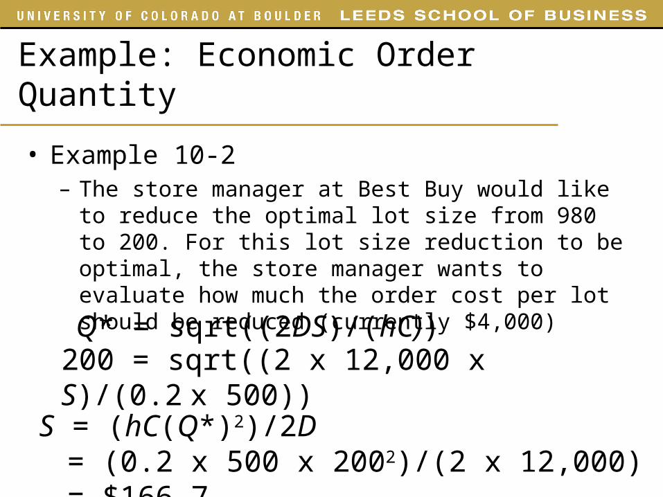
Example: Economic Order Quantity

• Example 10-2– The store manager at Best Buy would like to reduce the

optimal lot size from 980 to 200. For this lot size reduction to be optimal, the store manager wants to evaluate how much the order cost per lot should be reduced (currently $4,000)

Q* = sqrt((2DS)/(hC))200 = sqrt((2 x 12,000 x S)/(0.2 x 500))

S = (hC(Q*)2)/2D= (0.2 x 500 x 2002)/(2 x 12,000) = $166.7

Example: Economic Order Quantity

• How can the store manager reduce the fixed ordering cost?– Aggregate multiple products in a single order

• Can possibly combine shipments of different products from the same supplier

• Can also have a single delivery coming from multiple suppliers

Aggregating replenishment across products in a single order allows for a reduction in lot size for individual products because fixed ordering and transportation

cost are now spread across multiple products

Lot Sizing with Multiple Products or Customers

• Multiple products– Independent orders

• No aggregation: Each product ordered separately

– Joint order of all products• Complete aggregation: All products delivered on each

truck

– Joint order of a subset of products• Tailored aggregation: Selected subsets of products on

each truck

1 2 3

1 2 3

1 1 1

1 2 3 1 2 3

2 32

Which option will likely have the lowest cost?

Aggregating Replenishment Across Products

• Ordering cost has two components– Common (to all products)– Individual (to each product)

• Example– It is cheaper for Wal-Mart to receive a truck containing

a single product than a truck containing many different products

• Inventory and restocking effort is much less for a single product

Lot Sizing with Multiple Products or Customers

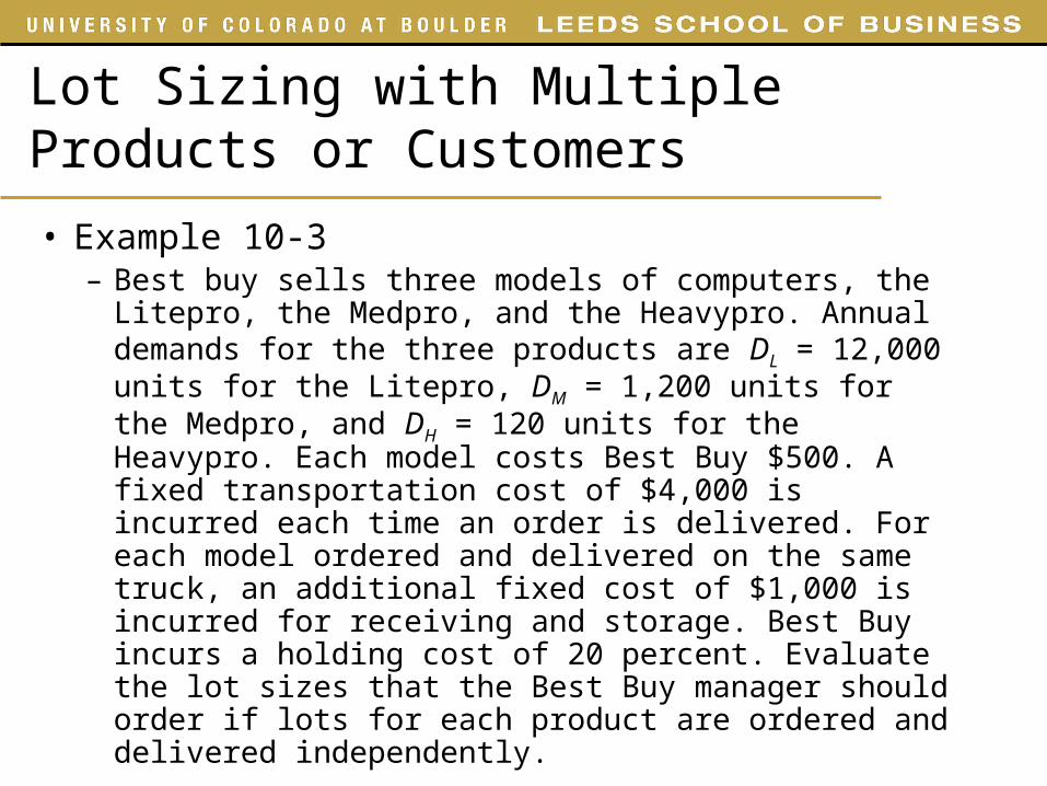
• Example 10-3– Best buy sells three models of computers, the Litepro,

the Medpro, and the Heavypro. Annual demands for the three products are DL = 12,000 units for the Litepro, DM = 1,200 units for the Medpro, and DH = 120 units for the Heavypro. Each model costs Best Buy $500. A fixed transportation cost of $4,000 is incurred each time an order is delivered. For each model ordered and delivered on the same truck, an additional fixed cost of $1,000 is incurred for receiving and storage. Best Buy incurs a holding cost of 20 percent. Evaluate the lot sizes that the Best Buy manager should order if lots for each product are ordered and delivered independently.

Independent Orders

• Ordering cost is considered independent for each product– Apply EOQ to each product

Independent Orders

• Example 10-3– DL = 12,000 (demand per year)

– DM = 1,200

– DH = 120

– S = $4,000 (common order cost)

– sL = sM = sH = $1,000 (product specific order cost)

– h = 0.2 (holding cost)

– cL = cM = cH = $500 (material cost)

Independent Orders

Litepro Medpro Heavypro

Demand per year D 12,000 1,200 120

Fixed cost/order S $5,000 $5,000 $5,000

Optimal order size Q* 1,095

Cycle inventory Q/2 548

Order frequency n* 11.0/year

Average flow time 2.4 weeks

Annual holding cost $54,772

Annual order cost $54,772

Total cost $109,544

Total cost = $155,140

110

55

1.1/year

23.7 weeks

$5,477

$5,477

$10,945

1 2 3

346

173

3.5/year

7.5 weeks

$17,321

$17,321

$34,642

H

SDEOQ

2

hCQ*

Joint Orders of all Products

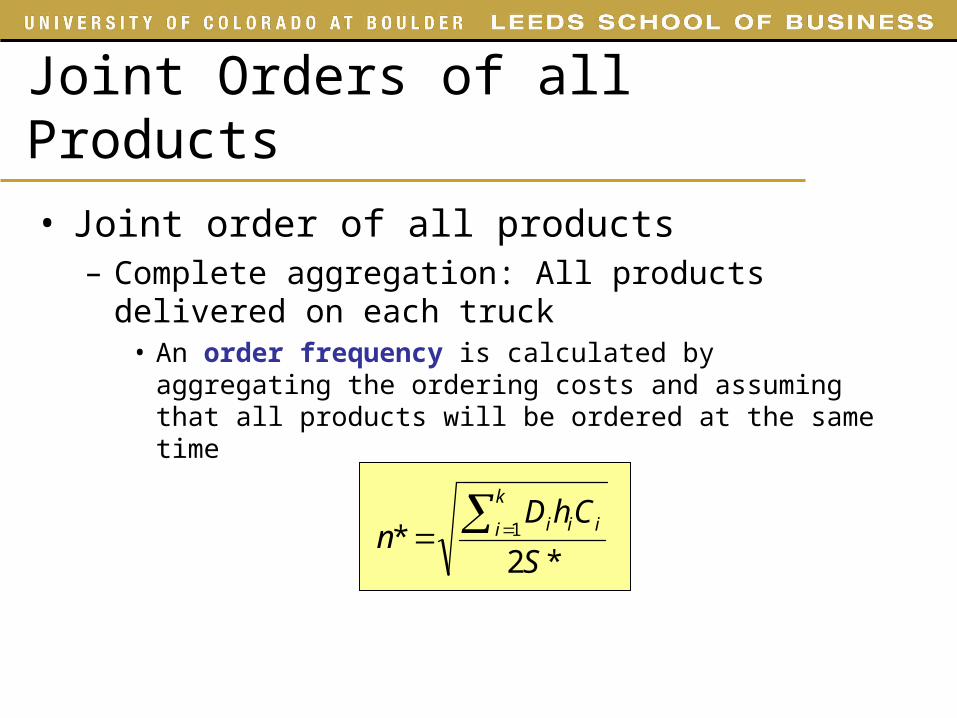
• Joint order of all products– Complete aggregation: All products delivered on each

truck • An order frequency is calculated by aggregating the

ordering costs and assuming that all products will be ordered at the same time

Supply Chain Cost Influenced by Lot Size

Holding cost(Q1/2)H1 + (Q2/2)H2 + (Q3/2)H3

Material costC1D1 + C2D2 + C3D3

Order quantity

Order cost(D1/Q1)S + (D2/Q2)S + (D3/Q3)S

Annual cost

Supply Chain Cost Influenced by Lot Size

Holding cost(D1/2n)H1 + (D2/2n)H2 + (D3/2n)H3

Order quantity

Order costnS*

Annual cost

Material costC1D1 + C2D2 + C3D3

Joint Orders of all Products

• Joint order of all products– Complete aggregation: All products delivered on each

truck • An order frequency is calculated by aggregating the

ordering costs and assuming that all products will be ordered at the same time

*2* 1

S

ChDn

k

i iii

Joint Orders of all Products

• Inputs– DL = 12,000 (demand per year)– DM = 1,200– DH = 120– S = $4,000 (common order cost)– sL = sM = sH = $1,000 (product specific order cost)– h = 0.2 (holding cost)– cL = cM = cH = $500 (material cost)

• S* = S + sL + sM + sH = $7000• n* = SQRT((DLhCL+ DMhCM + DHhCH)/2S*) = 9.75• QL = DL/n* = 12000/9.75 = 1230• QM = DM/n* = 1200/9.75 = 123• QH = DH/n* = 120/9.75 = 12.3

*2* 1

S

ChDn

k

i iii

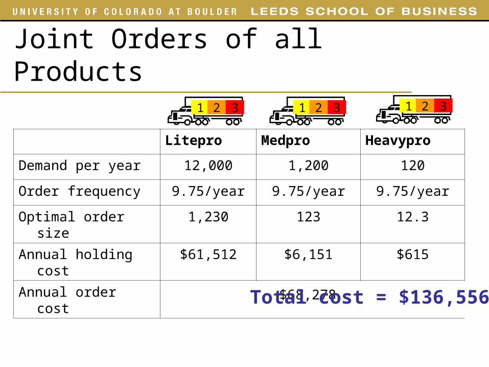
Joint Orders of all Products

Litepro Medpro Heavypro

Demand per year 12,000 1,200 120

Order frequency 9.75/year 9.75/year 9.75/year

Optimal order size 1,230 123 12.3

Annual holding cost $61,512 $6,151 $615

Annual order cost $68,278

Total cost = $136,556

1 2 3 1 2 3 1 2 3

Joint Order of a Subset of Products

• Joint order do not include all products• Ordering frequency may be different for each

product– It is based on the product that has the highest

frequency

Total cost = $130,767

Lessons From Aggregation

• Complete aggregation is effective if product specific fixed cost is a small fraction of joint fixed cost

• Tailored aggregation is effective if product specific fixed cost is a large fraction of joint fixed cost

EOQ in Practice

• 1961 survey– A majority cited “pure judgment” as the method for determining

inventory ordering

• 1973 survey– 56% of the respondents were using EOQ

• 1978 survey– 85% of the respondents were using EOQ

• 1983 survey– 57% of the respondents were using EOQ

• 2007 textbook– “The EOQ is extremely valuable, but it is rarely used in

practice because of the difficulty in implementing it and capturing the requirement elements”

EOQ in Practice

• Criticism– Difficult to accurately estimate holding and ordering

costs– Demand is assumed to be constant– Lead time is assumed to be zero or constant– Order is assumed to arrive in one batch at one point in

time– Costs are assumed stationary– Quantity discounts are not possible (basic EOQ)

Measuring Demand Uncertainty

Inventory

Time

CycleInventory

CycleLead time (L)

Reorder point (ROP)

Demand (D)Order quantity/lot size (Q)

Measuring Demand Uncertainty

Inventory

Time

AverageInventory

CycleInventory

SafetyInventory

CycleLead time (L)

Reorder point (ROP)

Demand (D)Order quantity/lot size (Q)

What is Safety Inventory?

• Safety inventory– Safety inventory is inventory carried for the purpose of

satisfying demand that exceeds the amount forecasted for a given period

– Safety inventory is the average inventory remaining when the replenishment lot arrives

Role of Safety Inventory

• There is a fundamental tradeoff– Raising the level of safety inventory provides higher

levels of product availability and customer service– Raising the level of safety inventory also raises the

level of average inventory and therefore increases holding costs

Two Key Questions when Planning Safety Inventory

1. What is the appropriate level of safety inventory to carry?

2. What actions can be taken to improve product availability while reducing safety inventory?

Determining Appropriate Level of Safety Inventory

• The appropriate level of safety inventory is determined by the following three factors1. The uncertainty of both demand and supply

– Higher levels of uncertainty require higher levels of safety inventory

2. The desired level of product availability– Higher levels of desired product availability require

higher levels of safety inventory

3. The replenishment policy– Different replenishment policies lead to different

levels of safety inventory

Measuring Demand Uncertainty

Inventory

Time

AverageInventory

CycleInventory

SafetyInventory

CycleLead time (L)

Reorder point (ROP)

Demand (D)

Demand during lead time DL = LD

Order quantity/lot size (Q)

Standard deviation of demand over lead time L = (L)D

Measuring Product Availability

1. Cycle service level (CSL)• Fraction of replenishment cycles that end with all

customer demand met

2. Product fill rate (fr)• Fraction of demand that is satisfied from product in

inventory• Probability that product demand is supplied from

available inventory

3. Order fill rate• Fraction of orders that are filled from available

inventory

CSL and fr are different!

CSL is 0%, fill rate is almost 100%inventory

time0

CSL is 0%, fill rate is almost 0% inventory

time0

Replenishment Policies

• Continuous review – Inventory is continuously

monitored and an order of size Q is placed when the inventory level reaches the reorder point (ROP)

• Periodic review– Inventory is checked at regular

(periodic) intervals and an order is placed to raise the inventory to a specified threshold, the order-up-to level (OUL)

Safety Inventory

“RFID reduced Out-of-Stocks by 30 percent for products selling between 0.1 and 15 units a day

at Wal-Mart”

What actions can be taken to improve product availability while reducing safety inventory?

Why is it that successful retailers and manufacturers (i.e. Wal-Mart, Seven-Eleven Japan, Dell) carry only little inventory but still have high levels of product

availability?

Continuous Review Policy: Safety Inventory and Cycle Service LevelL: Lead time for replenishment

D: Average demand per unit time

D:Standard deviation of demand per period

DL: Mean demand during lead time

L: Standard deviation of demand during lead time

CSL: Cycle service level

ss: Safety inventory

ROP: Reorder point),,(

)(1

LL

L

LS

DL

L

DD

F

D

ROPFCSL

ssROP

CSLss

L

DL

Average Inventory = Q/2 + ss