Supply and Demand in the Market for Money: The Liquidity PreferenceFramework

Whereas the loanable funds framework determines the equilibrium interest rateusing the supply of and demand for bonds, an alternative model developed byJohn Maynard Keynes, known as the liquidity preference framework, deter-mines the equilibrium interest rate in terms of the supply of and demand formoney. Although the two frameworks look different, the liquidity preferenceanalysis of the market for money is closely related to the loanable funds frame-work of the bond market.1

The starting point of Keynes’s analysis is his assumption that there aretwo main categories of assets that people use to store their wealth: money andbonds. Therefore, total wealth in the economy must equal the total quantityof bonds plus money in the economy, which equals the quantity of bonds sup-plied Bs plus the quantity of money supplied Ms. The quantity of bonds Bd andmoney Md that people want to hold and thus demand must also equal the totalamount of wealth because people cannot purchase more assets than their avail-able resources allow. The conclusion is that the quantity of bonds and moneysupplied must equal the quantity of bonds and money demanded:

Bs � Ms � Bd � Md (1)

Collecting the bond terms on one side of the equation and the money termson the other, this equation can be rewritten as

Bs � Bd � Ml � Ms (2)

A P P E N D I X 4 T O C H A P T E R 4

W-29

1Note that the term market for money refers to the market for the medium of exchange,money. This market differs from the money market referred to by finance practitioners, whichis the financial market in which short-term debt instruments are traded.

The rewritten equation tells us that if the market for money is in equilibrium (Ms �Md), the right-hand side of Equation 2 equals zero, implying that Bs � Bd, meaningthat the bond market is also in equilibrium.

Thus it is the same to think about determining the equilibrium interest rate byequating the supply and demand for bonds or by equating the supply and demand formoney. In this sense, the liquidity preference framework, which analyzes the mar-ket for money, is equivalent to the loanable funds framework, which analyzes the bondmarket. In practice, the approaches differ because by assuming that there are onlytwo kinds of assets, money and bonds, the liquidity preference approach implicitlyignores any effects on interest rates that arise from changes in the expected returnson real assets such as automobiles and houses. In most instances, both frameworksyield the same predictions.

The reason that we approach the determination of interest rates with bothframeworks is that the loanable funds framework is easier to use when analyzingthe effects from changes in expected inflation, whereas the liquidity preferenceframework provides a simpler analysis of the effects from changes in income, theprice level, and the supply of money.

Because the definition of money that Keynes used includes currency (whichearns no interest) and checking account deposits (which in his time typically earnedlittle or no interest), he assumed that money has a zero rate of return. Bonds, theonly alternative asset to money in Keynes’s framework, have an expected return equalto the interest rate i.2 As this interest rate rises (holding everything else unchanged),the expected return on money falls relative to the expected return on bonds, and thiscauses the demand for money to fall.

We can also see that the demand for money and the interest rate should be nega-tively related by using the concept of opportunity cost, the amount of interest(expected return) sacrificed by not holding the alternative asset—in this case, a bond.As the interest rate on bonds i rises, the opportunity cost of holding money rises, andso money is less desirable and the quantity of money demanded must fall.

Figure 1 shows the quantity of money demanded at a number of interest rates,with all other economic variables, such as income and the price level, held constant.At an interest rate of 25%, point A shows that the quantity of money demanded is$100 billion. If the interest rate is at the lower rate of 20%, the opportunity cost ofmoney is lower, and the quantity of money demanded rises to $200 billion, as indi-cated by the move from point A to point B. If the interest rate is even lower, the quan-tity of money demanded is even higher, as is indicated by points C, D, and E. The curveMd connecting these points is the demand curve for money, and it slopes downward.

At this point in our analysis, we will assume that a central bank controls theamount of money supplied at a fixed quantity of $300 billion, so the supply curvefor money Ms in the figure is a vertical line at $300 billion. The equilibrium wherethe quantity of money demanded equals the quantity of money supplied occurs at theintersection of the supply and demand curves at point C, where

Md � Ms (3)

The resulting equilibrium interest rate is at i* � 15%.

W-30 Appendix 4 to Chapter 4

2Keynes did not actually assume that the expected returns on bonds equaled the interest rate butrather argued that they were closely related. This distinction makes no appreciable difference in ouranalysis.

We can again see that there is a tendency to approach this equilibrium by firstlooking at the relationship of money demand and supply when the interest rate is abovethe equilibrium interest rate. When the interest rate is 25%, the quantity of moneydemanded at point A is $100 billion, yet the quantity of money supplied is $300 bil-lion. The excess supply of money means that people are holding more money thanthey desire, so they will try to get rid of their excess money balances by trying to buybonds. Accordingly, they will bid up the price of bonds, and as the bond price rises,the interest rate will fall toward the equilibrium interest rate of 15%. This tendency isshown by the downward arrow drawn at the interest rate of 25%.

Likewise, if the interest rate is 5%, the quantity of money demanded at point Eis $500 billion, but the quantity of money supplied is only $300 billion. There is nowan excess demand for money because people want to hold more money than theycurrently have. To try to get the money, they will sell their only other asset—bonds—and the price will fall. As the price of bonds falls, the interest rate will rise toward theequilibrium rate of 15%. Only when the interest rate is at its equilibrium value willthere be no tendency for it to move further, and the interest rate will settle to its equi-librium value.

Changes in Equilibrium Interest Rates Analyzing how the equilibrium interest rate changes using the liquidity preferenceframework requires that we understand what causes the demand and supply curvesfor money to shift.

Supply and Demand in the Market for Money: The Liquidity Preference Framework W-31

5

10

20

25

30

0 200 300 400 600500

i * = 15

Quantity of Money, M($ billions)

M s

M d

100

Interest Rate, i( % )

A

B

C

D

E

Figure 1 Equilibrium in the Market for Money

Shifts in the Demand for MoneyIn Keynes’s liquidity preference analysis, two factors cause the demand curve formoney to shift: income and the price level.

Income Effect In Keynes’s view, there were two reasons why income would affectthe demand for money. First, as an economy expands and income rises, wealthincreases and people will want to hold more money as a store of value. Second, as theeconomy expands and income rises, people will want to carry out more transac-tions using money, with the result that they will also want to hold more money. Theconclusion is that a higher level of income causes the demand for money to

increase and the demand curve to shift to the right.

Price-Level Effect Keynes took the view that people care about the amount of moneythey hold in real terms, that is, in terms of the goods and services that it can buy.When the price level rises, the same nominal quantity of money is no longer as valu-able; it cannot be used to purchase as many real goods or services. To restore their hold-ings of money in real terms to its former level, people will want to hold a greater nominalquantity of money, so a rise in the price level causes the demand for money

to increase and the demand curve to shift to the right.

Shifts in the Supply of MoneyWe will assume that the supply of money is completely controlled by the central bank,which in the United States is the Federal Reserve. (Actually, the process that deter-mines the money supply is substantially more complicated and involves banks, depos-itors, and borrowers from banks. We will study it in more detail later in the book.) Fornow, all we need to know is that an increase in the money supply engineered

by the Federal Reserve will shift the supply curve for money to the right.

CASE

Changes in the Equilibrium InterestRate Due to Changes in Income, the Price Level, or the Money Supply

To see how the liquidity preference framework can be used to analyze the movementof interest rates, we will again look at several cases that will be useful in evaluatingthe effect of monetary policy on interest rates. (As a study aid, Table 1 summarizesthe shifts in the demand and supply curves for money.)

W-32 Appendix 4 to Chapter 4

Learning the liquidity preference framework also requires practicing applications. Whenthere is a case in the text to examine how the interest rate changes because some economicvariable increases, see if you can draw the appropriate shifts in the supply and demandcurves when this same economic variable decreases. And remember to use the ceterisparibus assumption: When examining the effect of a change in one variable, hold all othervariables constant.

study guide

Changes in IncomeWhen income is rising during a business cycle expansion, we have seen that thedemand for money will rise. It is shown in Figure 2 by the shift rightward in the demandcurve from to The new equilibrium is reached at point 2 at the intersec-tion of the curve with the money supply curve Ms. As you can see, the equilibriuminterest rate rises from i1 to i2. The liquidity preference framework thus generates theconclusion that when income is rising during a business cycle expansion

(holding other economic variables constant), interest rates will rise. Thisconclusion is unambiguous when contrasted to the conclusion reached about theeffects of a change in income on interest rates using the loanable funds framework.

Changes in the Price LevelWhen the price level rises, the value of money in terms of what it can purchase islower. To restore their purchasing power in real terms to its former level, peoplewill want to hold a greater nominal quantity of money. A higher price level shifts

M 2 d

M 2 dM 1

d

Supply and Demand in the Market for Money: The Liquidity Preference Framework W-33

Change in Change in Money Demand [Md] Change inVariable Variable or Supply [Ms] Interest Rate

Income ↑ Md↑ ↑

Price level ↑ Md↑ ↑

Money supply ↑ Ms↑ ↓

Note: Only increases (↑) in the variables are shown. The effect of decreases in the variables on the change in demand or supplywould be the opposite of those indicated in the remaining columns.

Table 1 Summary Factors That Shift the Demand for and Supply of Money

i

M

Ms

i2

i1

i

M

i1i2

Md1

Md2

Ms1 Ms

2

←

←

i

M

Ms

i2

i1

Md1

Md2

←

Md

the demand curve for money to the right from to (see Figure 3). The equi-librium moves from point 1 to point 2, where the equilibrium interest rate has risenfrom i1 to i2, illustrating that when the price level increases, with the supply of

money and other economic variables held constant, interest rates will rise.

M 2 dM 1

d

W-34 Appendix 4 to Chapter 4

Md1

Md2

2

1

i 2

i 1

M

Interest Rate, i

Quantity of Money, M

Ms

Figure 2 Response to a Change in Income

In a business cycle expansion, when income is rising, the demand curve shifts fromto . The supply curve is fixed at . The equilibrium interest rate risefrom i1 to i2.

M s � MM 2 d

M 1 d

Md1

Md2

2

1

i 2

i 1

M

Interest Rate, i

Quantity of Money, M

Ms

Figure 3 Response to a Change in the Price Level

An increase in price level shifts the money demand curve from to , and the equi-librium interest rate rises from i1 to i2.

M 2 dM 1

d

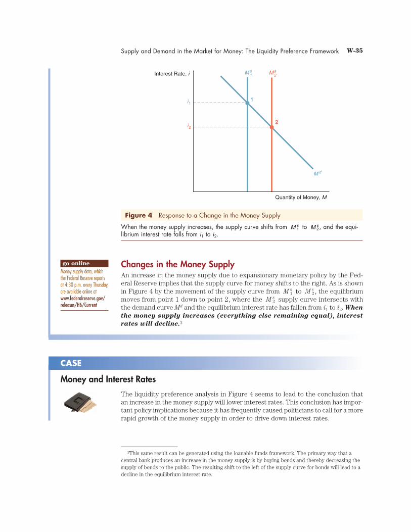
Changes in the Money SupplyAn increase in the money supply due to expansionary monetary policy by the Fed-eral Reserve implies that the supply curve for money shifts to the right. As is shownin Figure 4 by the movement of the supply curve from to , the equilibriummoves from point 1 down to point 2, where the supply curve intersects withthe demand curve Md and the equilibrium interest rate has fallen from i1 to i2. When

the money supply increases (everything else remaining equal), interest

rates will decline.3

CASE

Money and Interest Rates

The liquidity preference analysis in Figure 4 seems to lead to the conclusion thatan increase in the money supply will lower interest rates. This conclusion has impor-tant policy implications because it has frequently caused politicians to call for a morerapid growth of the money supply in order to drive down interest rates.

M 2 s

M 2 sM 1

s

Supply and Demand in the Market for Money: The Liquidity Preference Framework W-35

Quantity of Money, M

Ms1 Ms

2

2

1

i 2

i 1

Interest Rate, i

M d

Figure 4 Response to a Change in the Money Supply

When the money supply increases, the supply curve shifts from to , and the equi-librium interest rate falls from i1 to i2.

M 2 sM 1

s

3This same result can be generated using the loanable funds framework. The primary way that acentral bank produces an increase in the money supply is by buying bonds and thereby decreasing thesupply of bonds to the public. The resulting shift to the left of the supply curve for bonds will lead to adecline in the equilibrium interest rate.

go online

Money supply data, whichthe Federal Reserve reportsat 4:30 p.m. every Thursday,are available online atwww.federalreserve.gov/releases/H6/Current

But is this conclusion that money and interest rates should be negatively relatedcorrect? Might there be other important factors left out of the liquidity preferenceanalysis in Figure 4 that would reverse this conclusion? We will provide answers tothese questions by applying the supply and demand analysis we have learned in thischapter to obtain a deeper understanding of the relationship between money andinterest rates.

An important criticism of the conclusion that a rise in the money supply lowersinterest rates has been raised by Milton Friedman, a Nobel laureate in economics. Heacknowledges that the liquidity preference analysis is correct and calls the result—that an increase in the money supply (everything else remaining equal) lowersinterest rates—the liquidity effect. However, he views the liquidity effect as merelypart of the story: An increase in the money supply might not leave “everything elseequal” and will have other effects on the economy that may make interest rates rise.If these effects are substantial, it is entirely possible that when the money supplyrises, interest rates too may rise.

We have already laid the groundwork to discuss these other effects because wehave shown how changes in income, the price level, and expected inflation affectthe equilibrium interest rate.

1. Income effect. Because an increasing money supply is an expansionary influenceon the economy, it should raise national income and wealth. Both the liquiditypreference and loanable funds frameworks indicate that interest rates will thenrise (see Figure 2). Thus the income effect of an increase in the money

supply is a rise in interest rates in response to the higher level of

income.

2. Price-level effect. An increase in the money supply can also cause the overallprice level in the economy to rise. The liquidity preference framework predictsthat this will lead to a rise in interest rates. So the price-level effect from an

increase in the money supply is a rise in interest rates in response

to the rise in the price level.

3. Expected-inflation effect. The rising price level (the higher inflation rate) thatresults from an increase in the money supply also affects interest rates by affect-ing the expected inflation rate. Specifically, an increase in the money supply maylead people to expect a higher price level in the future—hence the expected infla-tion rate will be higher. The loanable funds framework has shown us that thisincrease in expected inflation will lead to a higher level of interest rates. Therefore,the expected-inflation effect of an increase in the money supply is a

rise in interest rates in response to the rise in the expected inflation rate.

At first glance it might appear that the price-level effect and the expected-infla-tion effect are the same thing. They both indicate that increases in the price levelinduced by an increase in the money supply will raise interest rates. However, there

W-36 Appendix 4 to Chapter 4

To get further practice with the loanable funds and liquidity preference frameworks, showhow the effects discussed here work by drawing the supply and demand diagrams thatexplain each effect. This exercise will also improve your understanding of the effect ofmoney on interest rates.

study guide

is a subtle difference between the two, and this is why they are discussed as two sep-arate effects.

Suppose that there is a onetime increase in the money supply today that leadsto a rise in prices to a permanently higher level by next year. As the price level risesover the course of this year, the interest rate will rise via the price-level effect. Onlyat the end of the year, when the price level has risen to its peak, will the price-leveleffect be at a maximum.

The rising price level will also raise interest rates via the expected-inflation effectbecause people will expect that inflation will be higher over the course of the year.However, when the price level stops rising next year, inflation and the expected infla-tion rate will fall back down to zero. Any rise in interest rates as a result of the ear-lier rise in expected inflation will then be reversed. We thus see that in contrast tothe price-level effect, which reaches its greatest impact next year, the expected-infla-tion effect will have its smallest impact (zero impact) next year. The basic differ-ence between the two effects, then, is that the price-level effect remains even afterprices have stopped rising, whereas the expected-inflation effect disappears.

An important point is that the expected-inflation effect will persist only as longas the price level continues to rise. A onetime increase in the money supply will notproduce a continually rising price level; only a higher rate of money supply growthwill. Thus a higher rate of money supply growth is needed if the expected-inflationeffect is to persist.

Does a Higher Rate of Growth of the MoneySupply Lower Interest Rates?We can now put together all the effects we have discussed to help us decide whetherour analysis supports the politicians who advocate a greater rate of growth of themoney supply when they feel that interest rates are too high. Of all the effects, onlythe liquidity effect indicates that a higher rate of money growth will cause a declinein interest rates. In contrast, the income, price-level, and expected-inflation effectsindicate that interest rates will rise when money growth is higher. Which of theseeffects are largest, and how quickly do they take effect? The answers are critical indetermining whether interest rates will rise or fall when money supply growth isincreased.

Generally, the liquidity effect from the greater money growth takes effect imme-diately because the rising money supply leads to an immediate decline in the equi-librium interest rate. The income and price-level effects take time to work becausethe increasing money supply takes time to raise the price level and income, whichin turn raise interest rates. The expected-inflation effect, which also raises interestrates, can be slow or fast, depending on whether people adjust their expectationsof inflation slowly or quickly when the money growth rate is increased.

Three possibilities are outlined in Figure 5; each shows how interest ratesrespond over time to an increased rate of money supply growth starting at time T.

Panel (a) shows a case in which the liquidity effect dominates the other effects sothat the interest rate falls from i1 at time T to a final level of i2. The liquidity effectoperates quickly to lower the interest rate, but as time goes by, the other effects startto reverse some of the decline. Because the liquidity effect is larger than the others,however, the interest rate never rises back to its initial level.

Panel (b) has a lesser liquidity effect than the other effects, with the expected-inflation effect operating slowly because expectations of inflation are slow to adjust

Supply and Demand in the Market for Money: The Liquidity Preference Framework W-37

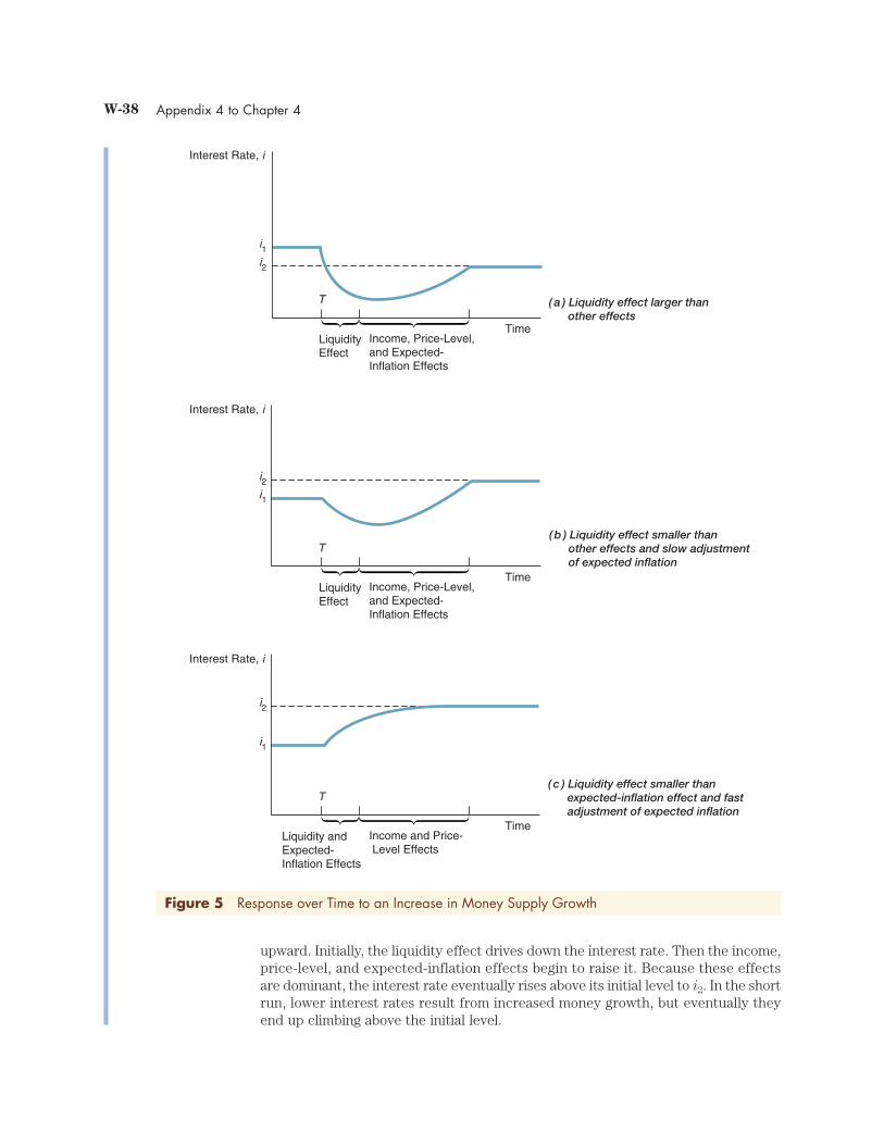
upward. Initially, the liquidity effect drives down the interest rate. Then the income,price-level, and expected-inflation effects begin to raise it. Because these effectsare dominant, the interest rate eventually rises above its initial level to i2. In the shortrun, lower interest rates result from increased money growth, but eventually theyend up climbing above the initial level.

W-38 Appendix 4 to Chapter 4

LiquidityEffect

Income, Price-Level,and Expected-Inflation Effects

( a ) Liquidity effect larger than other effects

Time

i1i2

T

LiquidityEffect

Income, Price-Level,and Expected-Inflation Effects

( b ) Liquidity effect smaller than other effects and slow adjustment of expected inflation

Time

i1

i2

T

Liquidity andExpected-Inflation Effects

Income and Price- Level Effects

( c ) Liquidity effect smaller than expected-inflation effect and fast adjustment of expected inflation

Time

i1

i2

T

Interest Rate, i

Interest Rate, i

Interest Rate, i

Figure 5 Response over Time to an Increase in Money Supply Growth

Panel (c) has the expected-inflation effect dominating as well as operatingrapidly because people quickly raise their expectation of inflation when the rate ofmoney growth increases. The expected-inflation effect begins immediately to over-power the liquidity effect, and the interest rate immediately starts to climb. Over time,as the income and price-level effects start to take hold, the interest rate rises evenhigher, and the eventual outcome is an interest rate that is substantially above theinitial interest rate. The result shows clearly that increasing money supply growthis not the answer to reducing interest rates but rather that money growth shouldbe reduced in order to lower interest rates!

An important issue for economic policymakers is which of these three scenar-ios is closest to reality. If a decline in interest rates is desired, then an increase inmoney supply growth is called for when the liquidity effect dominates the othereffects, as in panel (a). A decrease in money growth is appropriate if the other effectsdominate the liquidity effect and expectations of inflation adjust rapidly, as in panel(c). If the other effects dominate the liquidity effect but expectations of inflationadjust only slowly, as in panel (b), then whether you want to increase or decreasemoney growth depends on whether you care more about what happens in the shortrun or the long run.

Which scenario is supported by the evidence? The relationship of interest ratesand money growth from 1950 to 2004 is plotted in Figure 6. When the rate of moneysupply growth began to climb in the mid-1960s, interest rates rose, indicating thatthe liquidity effect was dominated by the price-level, income, and expected-infla-tion effects. By the 1970s, interest rates reached levels unprecedented in the periodafter World War II, as did the rate of money supply growth.

Supply and Demand in the Market for Money: The Liquidity Preference Framework W-39

Money Growth Rate (M2)

Interest Rate

1955 1960 1965 1970 1975 1980 19851985 1990 1995 2000 20051950

0

—2

—4

—6

2

4

6

8

10

12

14

16

18

22

20

InterestRate (%)

MoneyGrowth Rate(% annual rate)

2

—2

—4

4

6

8

10

12

14

0

Figure 6 Money Growth (M2, Annual Rate) and Interest Rates (Three-Month Treasury Bills), 1950–2004

Sources: Federal Reserve Bulletin, various years. Tables 1.1 line 6 and http://www.federalreserve.gov/releases/H15/data.htm

The scenario depicted in panel (a) of Figure 5 seems doubtful, and the case forlowering interest rates by raising the rate of money growth is much weakened. Youshould not find this too surprising. The rise in the rate of money supply growth in the1960s and 1970s is matched by a large rise in expected inflation, which would leadus to predict that the expected-inflation effect would be dominant. It is the most plau-sible explanation for why interest rates rose in the face of higher money growth. How-ever, Figure 6 does not really tell us which one of the two scenarios, panel (b) or panel(c) of Figure 5, is more accurate. It depends critically on how fast people’s expec-tations about inflation adjust. However, recent research using more sophisticatedmethods than just looking at a graph like Figure 6 does indicate that increased moneygrowth temporarily lowers short-term interest rates.4

W-40 Appendix 4 to Chapter 4

4See Lawrence J. Christiano and Martin Eichenbaum, “Identification and the Liquidity Effect of aMonetary Policy Shock,” in Business Cycles, Growth, and Political Economy, ed. Alex Cukierman,Zvi Hercowitz, and Leonardo Leiderman (Cambridge, Mass.: MIT Press, 1992), pp. 335–370; Eric M.Leeper and David B. Gordon, “In Search of the Liquidity Effect,” Journal of Monetary Economics 29(1992): 341–370; Steven Strongin, “The Identification of Monetary Policy Disturbances: Explaining the Liquidity Puzzle,” Journal of Monetary Economics 35 (1995): 463–497; and Adrian Pagan andJohn C. Robertson, “Resolving the Liquidity Effect,” Federal Reserve Bank of St. Louis Review 77(May–June 1995): 33–54.