1

Supplementary Information: Effect of the ambient conditions on the

operation of a large-area integrated photovoltaic-electrolyser

Erno Kemppainen, Stefan Aschbrenner, Fuxi Bao, Aline Luxa, Christian Schary, Radu Bors, Stefan

Janke, Iris Dorbandt, Bernd Stannowski, Rutger Schlatmann, Sonya Calnan

1. Irradiance and temperature dependency of PV performance The figures in this section show the irradiance and temperature dependency of the short circuit

current, maximum power point current and maximum power of a standalone silicon heterojunction

PV mini-module similar to the one used for the integrated photovoltaic electrolyser. The -0.013 W/°C

slope in Figure S1.6. corresponds to an efficiency reduction of about -0.044 %/°C (absolute), when

normalized with the total collection area of 294 cm2 and to about -0.056 %/°C (absolute) with the

active area of 228 cm2.

Figure S1.1. Irradiance dependency of the experimentally determined short circuit current of a silicon

heterojunction PV mini-module at a module temperature of 25 °C compared with a linear fit

extrapolated to 1000 W/m2

Electronic Supplementary Material (ESI) for Sustainable Energy & Fuels.This journal is © The Royal Society of Chemistry 2020

2

Figure S1.2. Temperature dependency of the experimentally determined short circuit current of a

silicon heterojunction PV mini-module at a fixed irradiance of 1000 W/m2

Figure S1.3. Irradiance dependency of the experimentally determined maximum power point current

(circles) at 25 °C compared with a linear fit extrapolated to 1000 W/m2

3

Figure S1.4. Temperature dependency of the experimentally determined maximum power point

current under 1000 W/m2 at 25–80 °C

Figure S1.5. Irradiance dependency of the experimentally determined maximum power compared with

a linear fit extrapolated to 1000 W/m2

4

Figure S1.6. Temperature dependency of the experimentally determined maximum power under 1000

W/m2 with a linear fit

2. HER and OER reaction kinetics Figure S2.1. shows the HER (a) and OER (b) reaction kinetics on plain Ni foam and on catalyst covered

Ni foam in 1.0 M KOH at 25 °C. In all cases a 5 cm × 6 cm graphite plate was used as the counter

electrode and Hg/HgO filled with 1.0 M KOH as the reference electrode (+0.927 V vs RHE at 25 °C 1,2).

Depending on the current density, both NiMo and NiFe show a circa 50–70 mV improvement over plain

Ni. The area immersed in the electrolyte is about 1.0 cm2 in all cases, and the pores leading to the rest

of the foam above the liquid are blocked with epoxy to prevent them from being in contact with the

electrolyte due to capillary effect.

Figure S2.1. The reaction kinetics of a) the HER and b) the OER in 1.0 M KOH at 25 °C using graphite

plate counter electrode and Hg/HgO reference electrode. In both cases plain NI foam is marked with

black, data as measured with solid lines and 100 % IR compensated with dashed lines. The red lines

correspond to the catalyst coated Ni foams, in a) NiMo and in b) NiFe.

5

3. Simulations for device development The geometry scheme is shown in Figure S3.1. In most cases the electrochemical kinetics parameters

that we used corresponded to the kinetics on Ni foam. Minimizing the electrode separation was

expectedly noticed to be an effective way to reduce resistive losses in the electrolyte and thus an

essential improvement in the design. Further improvements could have been gained by minimizing the

electrolyte volume around the electrode (i.e. small dX, dY, dZ), but we could not implement this change

in the design within the available time. This improvement would have been a combination of reduced

H2 and O2 transport losses and also reduced OH- transport losses (at high currents). The likely reason

for these improvements is that for a given electrolyte flow rate, the liquid velocity inside the

electrolyser would have been higher, sweeping the reaction products away and refreshing the KOH

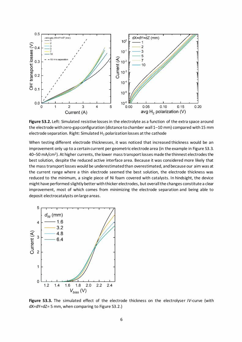
within the electrodes more efficiently. The slope of the OH- transport losses in Figure S3.2. a)(i.e.

resistive losses in the electrolyte and over the separator membrane) at less than 2.0 A indicates about

40–50 mΩ resistance for the zero-gap configurations, depending on the electrolyte volume.

Figure S3.1. The electrolyser geometry used in the simulations and the geometrical parameters

relating to the size of the electrolyser.

6

Figure S3.2. Left: Simulated resistive losses in the electrolyte as a function of the extra space around

the electrode with zero-gap configuration (distance to chamber wall 1–10 mm) compared with 15 mm

electrode separation. Right: Simulated H2 polarization losses at the cathode

When testing different electrode thicknesses, it was noticed that increased thickness would be an

improvement only up to a certain current per geometric electrode area (in the example in Figure S3.3.

40–50 mA/cm2). At higher currents, the lower mass transport losses made the thinnest electrodes the

best solution, despite the reduced active interface area. Because it was considered more likely that

the mass transport losses would be underestimated than overestimated, and because our aim was at

the current range where a thin electrode seemed the best solution, the electrode thickness was

reduced to the minimum, a single piece of Ni foam covered with catalysts. In hindsight, the device

might have performed slightly better with thicker electrodes, but overall the changes constitute a clear

improvement, most of which comes from minimizing the electrode separation and being able to

deposit electrocatalysts on large areas.

Figure S3.3. The simulated effect of the electrode thickness on the electrolyser IV-curve (with

dX=dY=dZ= 5 mm, when comparing to Figure S3.2.)

7

Figure S3.4. Simulated changes to the IV-curve from plain Ni electrodes at a 15 mm separation (legend:

15 mm) to a zero-gap design with minimized electrolyte volume (zero-gap, 1 mm), to reducing the

electrode thickness to a single foam sheet (dNi=1.6 mm) and depositing electrocatalysts on the Ni foams

(catalysts).

8

4. Outdoor and indoor measurement transients As mentioned in the article, the example transients shown in the article are not the only measurements

we did, and the other transients included in the analysis are shown here in chronological order. The 5-

minute averages correspond to the points in the scatter plots Figures 4 and 9–12, excluding points

when the device was covered and not operating. Except for the measurement on 29th August 2019,

the PV glass temperature was hotter than the electrolyte temperatures. The electrolyser inlets were

always hotter than outlets (not shown).

Figure S4.1. Time dependent profiles measured on 23rd July 2019 of a) H2 and O2 flow rates and solar irradiance. Flow rate transients are averaged over 60 seconds (lines) and 5 minutes (squares and circles) to reduce noise in the signal. b) Time dependent profiles measured on 23rd July 2019 of ambient, PV glass and electrolyte temperatures.

9

Figure S4.2. Time dependent profiles measured on 9th August 2019 of a) H2 and O2 flow rates and solar irradiance. Flow rate transients are averaged over 60 seconds (lines) and 5 minutes (squares and circles) to reduce noise in the signal. b) Time dependent profiles measured on 9th August 2019 of ambient, PV glass and electrolyte temperatures

Figure S4.3. Time dependent profiles measured on 29th August 2019 of a) H2 and O2 flow rates and solar irradiance. Flow rate transients are averaged over 60 seconds (lines) and 5 minutes (squares and circles) to reduce noise in the signal. b) Time dependent profiles measured on 29th August 2019 of ambient, PV glass and electrolyte temperatures.

10

Figure S4.4. Time dependent profiles measured on 22nd September 2019 of a) H2 and O2 flow rates and

solar irradiance. Flow rate transients are averaged over 60 seconds (lines) and 5 minutes (squares and

circles) to reduce noise in the signal. b) Time dependent profiles measured on 22nd September 2019 of

ambient, PV glass and electrolyte temperatures.

Figure S4.5. Time dependent profiles measured on 14th October 2019 of a) H2 and O2 flow rates and

solar irradiance. Flow rate transients are averaged over 60 seconds (lines) and 5 minutes (squares and

circles) to reduce noise in the signal. b) Time dependent profiles measured on 14th October 2019 of

ambient, PV glass and electrolyte temperatures.

11

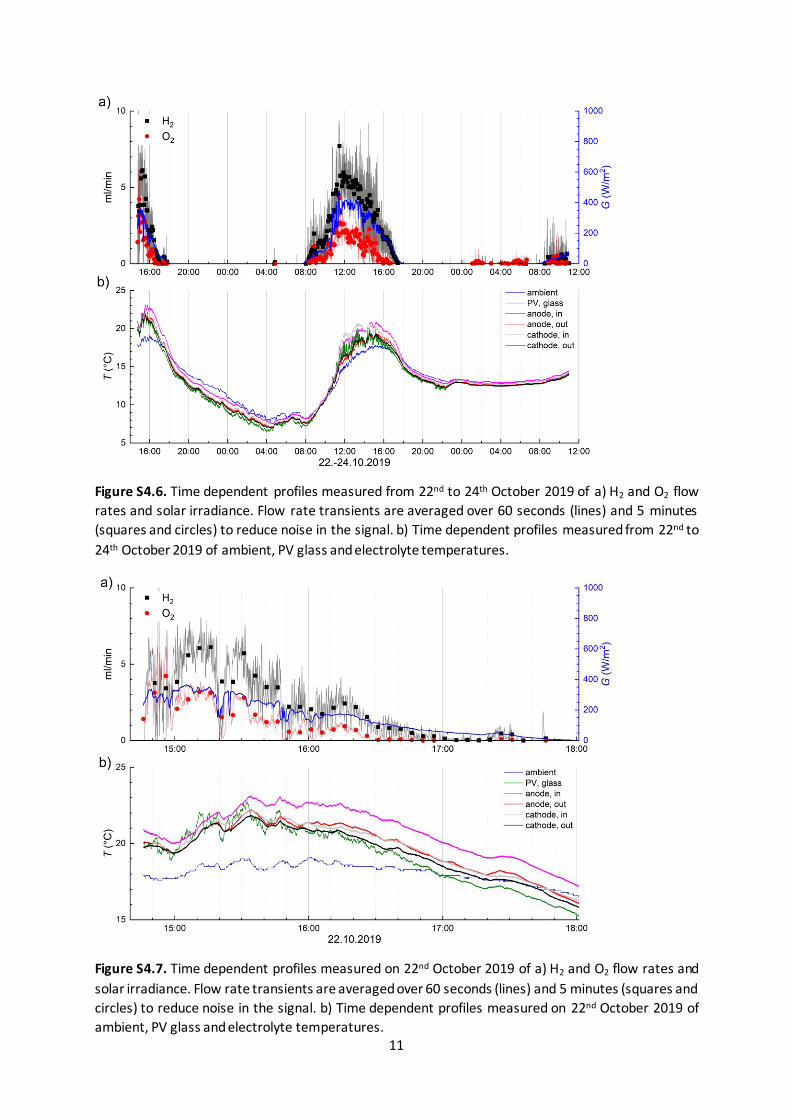
Figure S4.6. Time dependent profiles measured from 22nd to 24th October 2019 of a) H2 and O2 flow

rates and solar irradiance. Flow rate transients are averaged over 60 seconds (lines) and 5 minutes

(squares and circles) to reduce noise in the signal. b) Time dependent profiles measured from 22nd to

24th October 2019 of ambient, PV glass and electrolyte temperatures.

Figure S4.7. Time dependent profiles measured on 22nd October 2019 of a) H2 and O2 flow rates and

solar irradiance. Flow rate transients are averaged over 60 seconds (lines) and 5 minutes (squares and

circles) to reduce noise in the signal. b) Time dependent profiles measured on 22nd October 2019 of

ambient, PV glass and electrolyte temperatures.

12

Figure S4.8. Time dependent profiles measured on 23rd October 2019 of a) H2 and O2 flow rates and

solar irradiance and (b) ambient, PV glass and electrolyte temperatures.

Figure S4.9. Time dependent profiles from the first indoor measurement of a) H2 and O2 flow rates and

the irradiance setting of the solar simulator. Flow rate transients were averaged over 60 seconds (lines)

and 5 minutes (squares and circles) to reduce noise in the signal. b) Time dependent profiles measured

for ambient, PV and electrolyte temperatures.

13

For the illustration of the temperature distribution of the PV surface, we show a thermography image

in Figure S4.10. The recording was taken on 6th September 2019 at 9:55 (see also Figure 5). The PV

temperature transient indicated about 20 °C temperature, and the Pt 100 thermometer was placed at

the location indicated by the red “X”, corresponding to approximately 22–23 °C temperature, the

maximum temperature at a small spot being a little less than 27 °C, and 25–26 °C over a larger area.

At the time of recording, wind was blowing from southwest–west, probably contributing to the

nonsymmetric distribution.

Figure S4.10. Thermographic image of the PV glass surface taken at 09:55 on 6th September 2019

during outdoor exposure with the approximate cardinal directions. The outlets are to the left of the

figure, and inlets to the right. The edges and busbars of the PV cells are distinguishable as straight

lines (compare to Figure 1.). The slight distortion is due to perspective. The approximate location of

the temperature sensor is a marked with the red “X”. Cathode is above the horizontal centre line

(cutting the width axis at ca. 9 cm) and anode below it.

14

5. Supplementary graphs for the performance analysis Figure S5.1. shows the STH efficiency plotted against the PV temperature with the irradiance indicated

on the color scale. The slope of the outdoor points is roughly -0.23%/°C (absolute change in the STH

efficiency).

Figure S5.1. The STH efficiency as a function of PV temperature. Outdoor data marked with squares

(open squares 22.–24.10.2019), indoor with stars.

Figure S5.2. shows the hydrogen generation rate and STH efficiency as a function of the ambient

temperature and irradiance. The general pattern is similar to Figure 8., but the indoor measurements

are clearly shifted to cooler temperatures with respect to the outdoor measurements.

Figure S5.2. The STH efficiency as a function of the ambient temperature. Outdoor data marked with

squares (open squares 22.–24.10.2019), indoor with stars.

Figure S5.3. shows the STH efficiency as a function of ambient temperature with a logarithmic y-axis

to illustrate that the data would fit an exponential function as well as linear (compare with Figure 10).

The efficiency trend of equation (4) for the outdoor data is indicated with the dashed line.

15

Figure S5.3. The STH efficiency as a function of ambient temperature plotted with a logarithmic y-axis,

illustrating that the outdoors data would fit an exponential as well as a linear decrease. Outdoor data

marked with squares (open squares 22.–24.10.2019), indoor with stars.

The outflow ratio as a function of the cathodic outflow is shown in Figure S5.4. The general trend is

similar to using the anodic outflow as the x-axis, but the scatter of the data at low outflows is higher.

However, above ca. 10 ml/min the ratio seems to increase slightly, suggesting that low current density

could have contributed to the deviation from 2.0 outflow ratio.

Figure S5.4. The outflow ratio as the function of the cathodic outflow. Outdoor measurements marked

with solid markers, indoor with open circles.

The outflow ratio as a function of the ambient conditions is shown in Figure S5.5. Black markers

correspond to values less than 0.5 and grey to over 3.5. As can be seen, the outflow ratio increases as

irradiance decreases, and the ambient temperature does not seem to have obvious effects to the

outflow ratio. As mentioned related to Figure 10, the highest ratios occurred in the last outdoor

measurement, so degradation might also play a role, although later indoor the ratio was closer to 2.0.

16

Figure S5.5. The outflow ratio as a function of the ambient conditions. The black markers correspond

to values less than 0.5 and grey to more than 3.5.

References 1 S. Rondinini, P. Longhi, P. R. Mussini and T. Mussini, Pure Appl. Chem., 1994, 66, 641–647.

2 J. R. Swierk, S. Klaus, L. Trotochaud, A. T. Bell and T. D. Tilley, J. Phys. Chem. C, 2015, 119, 19022–19029.