Supplemental Digital Content 1 Mechanical power and the...

1

Supplemental Digital Content 1

Mechanical power and the development of Ventilator-Induced Lung

Injury

Massimo Cressoni, Miriam Gotti, Chiara Chiurazzi, Dario Massari, Ilaria Algieri, Martina Amini,

Antonio Cammaroto, Matteo Brioni, Klodiana Nikolla, Mariateresa Guanziroli, Daniele

Dondossola, Stefano Gatti, Vincenza Valerio, Paola Pugni, Paolo Cadringher, Nicoletta Gagliano,

Luciano Gattinoni

2

TABLE OF CONTENTS

SUPPLEMENTAL DIGITAL CONTENT 1 ................................................................................................. 1

MECHANICAL POWER AND THE DEVELOPMENT OF VENTILATOR-INDUCED LUNG

INJURY ............................................................................................................................................................. 1

STUDY PROTOCOL – ADDITIONAL METHODS ................................................................................... 4

Hemodynamic protocol ........................................................................................................................ 5

Data collection and computation ......................................................................................................... 5

Sacrifice and autopsy ........................................................................................................................... 6

Light microscopy .................................................................................................................................. 7

Wet to dry ratio .................................................................................................................................... 8

Lung Computed Tomography............................................................................................................... 9

Quantitative analysis of CT scan ..................................................................................................... 9

Piglet lung acinus size determination for inhomogeneity analysis ................................................ 10

Lung inhomogeneities determination4 ........................................................................................... 11

ENERGY COMPUTATIONS PER BREATH ................................................................................... 12

Relationship between total delivered energy to the respiratory system components .................... 13

Remove energy spent to move chest wall ...................................................................................... 16

Airways dissipated energy during inspiration – ex-vivo setting .................................................... 18

Energy dissipated in overcoming endotracheal tube/tracheobronchial tree resistances during

expiration ....................................................................................................................................... 19

3

Energy recoverable at mouth during tidal ventilation .................................................................... 20

Static dissipated energy into the respiratory system ...................................................................... 21

ENERGY PER BREATH AS FUNCTION OF FLOW AND TIDAL VOLUME .................................... 23

Total delivered energy to the respiratory system ........................................................................... 24

Delivered dynamic transpulmonary energy ................................................................................... 25


inspiration....................................................................................................................................... 26

Energy dissipated in overcoming endotracheal tube/tracheobronchial tree with tube of diameter

of 6 or 8 mm ................................................................................................................................... 27

RELATIONSHIPS BETWEEN THE DIFFERENT ENERGY COMPUTATIONS .............................. 28

SUPPLEMENTARY DATA FROM THE MAIN EXPERIMENTS ........................................................ 29

Equations of linear regressions in Table 1 e Table 2 (main text) .................................................. 29

Regressions for Figure 4 (main text).............................................................................................. 34

THRESHOLDS CALCULATION ........................................................................................................ 35

Estimation of delivered dynamic transpulmonary energy load threshold on tidal volume delivered

at respiratory rate of 15 breaths/minute ......................................................................................... 36

Relationships between increase of stress relaxation (P1-P2 cmH2O) and VILI development ........ 39

HISTOLOGY ............................................................................................................................................. 40

SUPPLEMENTAL REFERENCES ............................................................................................................. 40

4

Study protocol – additional methods

Anesthesia was induced with an intramuscular injection of medetomidine 0.025 mg/kg and

tiletamine/zolazepam 5 mg/kg. Thereafter, we cannulated an auricular vein. Keeping the animal

prone, after pre-oxygenation, we inserted an endotracheal tube (internal diameter 6 mm) and started

mechanical ventilation. During surgical preparation, mechanical ventilation was set in volume-

controlled mode (FiO2 0.5, Tidal Volume (VT) 10 ml/kg, respiratory rate 20-22 breaths/min in order

to obtain physiological EtCO2, Inspiratory : Expiratory ratio (I:E) 1:2, no post-inspiratory pause and

positive end-expiratory pressure (PEEP) 3-5 cmH2O.

Anesthesia was maintained with propofol 5-10 mg/kg/h, pancuronium bromide 0.3-0.5

mg/kg/h and midazolam 0.25-1 mg/kg/h. Normal saline (NaCl 0.9%) was administered at 100

ml/h during surgery, then 50 ml/h. Ceftriaxone 1 g i.v. and Tramadol 50 mg i.v. were

administered preoperatively, and every 12 hours during the study protocol. Low molecular

weight heparin 1900 IU s.c. was administered every 12 hours, after surgery. The animal was

turned supine for surgical preparation, carried out under sterile conditions, with piglet under

general anesthesia. Right carotid artery was exposed and cannulated. A three lumen central

venous catheter was inserted through the right internal jugular vein. A bladder catheter was

positioned via cistostomy. At the end of surgery, the animal was turned prone. After performing

gastric suction, a latex thin wall, 5 cm long, esophageal balloon was advanced in the inferior

third of the esophagus and filled-in with 1.5 ml of room air. Proper positioning of esophageal

balloon and endovascular catheters was later verified on thorax computed tomography (CT).

Pressure transducers were connected to the endotracheal tube, the esophageal balloon and the

endovascular catheters, zeroed at room air at heart level, as appropriate. Esophageal balloon

position was checked with CT scan.

5

Hemodynamic protocol

To maintain hemodynamic stability, a target mean arterial pressure (MAP) was set between

60 and 90 mmHg, with continuous saline infusion (50 ml/h). A fall in MAP below 60 mmHg was

corrected with 100-250 ml saline bolus and increases in saline infusion, up to 75-100 ml/h. If these

were not sufficient to restore the target MAP, norepinephrine (0.1-1.0 g/kg/min) was administered.

If MAP rose above 90 mmHg, hemodynamic support was deescalated. Cumulative fluid intake was

computed as the sum of fluids infused. Drugs were not included. Fluid balance was computed as

cumulative fluid intake minus total urinary output.

Data collection and computation

A complete data collection was performed every 6 hours. If respiratory mechanics or

hemodynamic variables changed (i.e. increase in peak/plateau pressure despite tracheal suctioning,

decrease in peripheral saturation, unexpected arterial hypotension or hypertension), data were also

collected. Prior to data collection and, in particular, before respiratory mechanics measurements,

tracheal suctioning was performed. VT, airways pressure and esophageal pressure were recorded

during tidal ventilation and during end-inspiratory and end-expiratory pauses.

Transpulmonary pressure was computed at end-inspiration as:

Transpulmonary pressure (cmH2O) = Airway pressure (cmH2O) – Esophageal pressure

(cmH2O)

Where:

Airway pressure (cmH2O) = Plateau airway pressure (cmH2O) – End expiratory pause

airway pressure (cmH2O)

Esophageal pressure (cmH2O) = Plateau esophageal pressure (cmH2O) – End expiratory

pause esophageal pressure (cmH2O)

Plateau airway and esophageal pressures were measured during a 5 seconds end-inspiratory pause.

Respiratory system (ERS), lung (EL) and chest wall (ECW) elastance were calculated as:

ERS = Airway pressure (cmH2O) /VT

6

EL = (Airway pressure (cmH2O) – Esophageal pressure (cmH2O)/VT

= Δ Transpulmonary pressure (cmH2O)/VT

ECW = Esophageal pressure (cmH2O)/VT

Arterial and central venous blood gases were analyzed (ABL825FLEX, Radiometer, Copenhagen,

Denmark®). Central venous pressure was measured during an end-expiratory pause. Internal body

temperature was measured. Elevations in body temperature (over 40.0 °C) were managed with

acetaminophen (15 mg/kg) and/or physical methods (ice in correspondence of femoral and axillary

arteries).

Data collection was completed with performance of 2 CT scans: the former was obtained during an

end-inspiratory pause, the latter during an end-expiratory pause.

Sacrifice and autopsy

After the scheduled 54 hours of the study, or before if whole lung edema developed, piglets

were sacrificed with a bolus injection of KCl 40 mEq i.v. under deep sedation (50 mg bolus dose of

propofol). After sacrifice, autopsy was performed. Chest was opened and lungs along with

tracheobronchial tree were excised and weighed.

7

Light microscopy

Figure 1: Histology. The colored areas represents the lung regions where lung fragments were collected for histological

analysis. Lung fragments for histological analysis were obtained from regions from 1 to 8. Three samples from

subpleural regions taken at the tips of the lobes (regions 1, 2, 3, 5, 6, 7) and one sample from the internal part of the

lung (regions 4 and 8).

Four regions in each lung were considered, as shown in Figure 1. Fragments were

immediately processed for morphological procedures by fixation in 4% formalin in 0.1 M

phosphate buffered saline (PBS), pH 7.4. After fixation lung fragments were routinely dehydrated,

paraffin embedded, and serially cut (thickness 5 m). For each specimen and for each staining we

analysed three slides obtained at a 100 m distance. Sections were stained with freshly made

haematoxylin-eosin to evaluate cells and tissue morphology. Haematoxylin-eosin stained sections

for each lung region were analysed at light microscope in blind by two independent operators using

a semi-quantitative grading scale to assess various features of the tissue. The variables included in

the scale for the analysis of lung structure and damage were: hyaline membranes formation,

diffusion and severity of interstitial and septal infiltrate, vascular congestion and intra-alveolar

haemorrhaging, alveoli rupturing and basophilic material deposition. Overall injury was expressed

by a scoring system from 0 to 4: 0) no alterations, 1) 25% of field involved; 2) 50 % of field

involved; 3) 75 % of field involved; 4) 50-100% of field involved.

8

Wet to dry ratio

Three samples from each lung (~ 1 cm3) were collected (upper, medium and lower lobe

respectively). They were immediately weighed and, after being dried for 24 hours at 50 °C, were

weighed again. Wet to dry ratio, that is an indicator of lung edema, was determined as the ratio

between the two measurements.

9

Lung Computed Tomography

Lung CT scans (Lightspeed, General Electric) were performed with the following settings:

- Collimation width: 32 x 2 x 0.6 mm

- Spiral pitch factor: 1.2

- Slice thickness: 5 mm

- Reconstruction interval: 5 mm

- Data collection FOV: 500 mm

- Reconstruction FOV: 300 mm

- KVp: 120

- X-Ray Tube Corrent: 110 mA

- Pixel dimensions: 0.585938/0.585938

- Acquisition matrix: 512 x 512

Quantitative analysis of CT scan

Lung profiles were manually drawn on each CT scan. Analysis was performed using a

dedicated software (SoftEFilm, Elekton, Italy), assuming the density of lung parenchyma to be

close to the density of water (0 HU). Each voxel can be analyzed assuming that it is made of two

compartments: air (-1000 HU) and lung tissue (including blood, 0 HU).

For each voxel, gas fraction was computed as follows:

Volume gas / (volume gas + volume tissue) = mean CT number observed / (CT number gas

– CT number tissue)

Rearranging:

Gas fraction = voxel density (Hounsfield units) / -1000

Tissue fraction = 1 – gas fraction

Consequently, gas and tissue volumes were defined as:

10

Gas volume = gas fraction x voxel volume

Tissue volume = tissue fraction x voxel volume

Voxel weight is equal to the tissue volume, assuming that tissue density is 1.

Aeration of lung parenchyma was classified in four subsets:

- Not inflated tissue: density > -100 HU

- Poorly inflated tissue: -500 HU < density < -100 HU

- Well inflated tissue: -900 HU < density < -500 HU

- Over inflated tissue: density < -900 HU

We defined “new densities” discrete regions of at least 6 mm (inner diameter of tracheal tube) of

maximal diameter with a density corresponding to poorly or not inflated tissue, not present in the

previous CT scan and distinguishable from the surrounding parenchyma. 2 We visually classified

the CT scan damage as follows:

Grade 0: baseline CT scan.

Grade 1: new densities clearly distinguishable from the surrounding parenchyma.

Grade 2: density occupying at least 1 lung field (apex-hilum-base and dependent/non

dependent).

Grade 3: density occupying all the 6 lung fields (whole lung edema).

Piglet lung acinus size determination for inhomogeneity analysis

As the ratio between airway space dimensions and animal weight follows a logarithmic scale

we estimated the acinar volume of piglets from the data presented by Sapoval and Weibel 3

reporting the acinus size in mouse, rat, rabbit and humans. For humans we used the 1/8 subacinus

since, as detailed by the authors, this 1/8 subacinus is more comparable to acini in other species and

computed an acinar volume of 12.1 mm3 corresponding to a radius of 1.42 mm.

11

Lung inhomogeneities determination4

CT scan images are composed by voxels whose dimensions depend both on the CT scan

hardware and on the setting for image reconstruction. We produced a lung inhomogeneities map

with dimensions 1:1 to the original CT scan map, but using as a “basic dimension” the acinar

volume and filtering the map with a gaussian filter with a radius equal to the radius of the acinus.

We obtained a CT value of each voxel which was dependent to the CT value of the neighboring

voxels. Around each voxel we defined a spherical crust starting at distance of one acinar radius

from the voxel center and of ½ acinar radius thickness. The ratio of the surrounding voxel gas to the

central voxel gas fraction indicates homogeneity if equal to 1, inhomogeneity when greater than 1.

We computed a vector of lung inhomogeneities dividing the filtered gas fraction in each of the

voxels included, at least partially, in the spherical crust, and the filtered value of the central voxel

and we wrote the maximum of the vector in the lung inhomogeneities map. While average is a

square filter and takes into the same account near and far voxels, gaussian filters exponentially

decreases weight of far voxels. We considered as stress raisers those points causing

inhomogeneities greater than 95th

percentile of the values observed in our normal piglets at baseline,

resulting in a threshold of 1.685. Lung inhomogeneity can be expressed as intensity (average ratio)

and extent (fraction of lung volume with inhomogeneities 1.685).

12

Energy computations per breath

Mechanical power = energy per breath times respiratory rate

The delivered energy per breath (airways + lung) was defined as the area between the inspiratory

limb of the -transpulmonary pressure (x) – volume curve and the volume axis (y) and was

measured in Joule (filled area in Figure 2 here below).

Figure 2: Dynamic (tidal breath) transpulmonary pressure-volume curve. An example of dynamic pressure-volume

curve (VT 750 ml, RR 6 bpm, I:E 1:2, no post-inspiratory pause).

Energy was computed on the pressure-volume graph:

Energy (N*m) = Pressure (N/m2) * Volume (m

3)

To convert cmH2O*ml in Joule:

1 J = 1 Pa * m3

1 Pa = 0.0101971621298 cmH2O

1 m3 = 1000000 ml

1 J = 0.0101971621298 cmH2O * 1000000 ml = 10197.16 cmH2O * ml

1 cmH2O * ml = 0.0000980665 J

Airways minus esophageal pressure (cmH2O)

Vo

lum

e (m

l)

0 10 20 30 40

0

200

400

600

800

1000

13

Relationship between total delivered energy to the respiratory system components

In order to analyze the relationships between the different components in which energy is spent

during tidal ventilation (see Figure 3), we performed additional measurements in six piglets. Before

the beginning of the study (i.e. when all animals’ lungs were still healthy), dynamic (i.e. during

tidal ventilation) and static pressure-volume curves were acquired at different combinations of VT

and RR. In the same animals, after autopsy, the same VT-RR combinations were used to acquire

pressure-volume curves on the isolated endotracheal tube/tracheobronchial tree. Below we reported

the combinations:

1) Dynamic pressure-volume curves, obtained during tidal ventilation:

◦ RR 15 breaths/min (I:E 1:2) and VT 150-300-450-600-750-900 ml, no post-inspiratory pause

◦ VT 450 ml and RR 3-6-9-12-15 breaths/min (I:E 1:2), no post-inspiratory pause.

2) Static pressure-volume curves, obtained with a super-syringe, as previously described:

◦ VT 150-300-450-600-750-900 ml

3) Airways pressure-volume curves, obtained during tidal ventilation of the endotracheal

tube/tracheobronchial tree as previously described:

◦ RR 3-6-9-12-15 breaths/min (I:E 1:2) and VT 150-300-450-600-750-900 ml: each possible

combination)

14

Energy delivered per breath to the respiratory system can be divided into different components

which are detailed in Figure 3. A detailed explanation of where energy is spent during mechanical

ventilation is relevant, as only the energy dissipated within the lung parenchyma may contribute to

Ventilator-Induced Lung Injury while the energy dissipated outside the lung should not contribute

to VILI. The use of esophageal pressure (see Figure 4) allows to remove the chest wall component.

We left the energy dissipated into the airways in the main text definition of mechanical power but

estimated the quota spent to overcome endotracheal tube and trachea (Figure 5-6 and 8). Figure 12-

13-14 demonstrate the dependency of all energy quotas on both flow and tidal volume. Figure 16

and 17 show that all the energies per breath we computed are related each other and that our results

would have been similar if a different definition of energy would have been used.

15

Figure 3: Definitions of components of total delivered energy to the respiratory system. In our hypothesis, when

the dissipated dynamic transalveolar energy overcomes the threshold, VILI occurs.

TOTAL DELIVERED ENERGY TO THE RESPIRATORY SYSTEM

Includes:

•Energy required to move the chest wall

•Energy dissipated in overcoming endotracheal tube/tracheobronchial tree during inspiration

•Dissipated dynamic transalveolar energy

•Energy dissipated in overcoming endotracheal tube/tracheobronchial tree during expiration

•Energy recoverable at mouth at the end of the respiratory cycle

DELIVERED DYNAMIC TRANSPULMONARY ENERGY

Includes:

•Energy dissipated in overcoming endotracheal tube/tracheobronchial tree during inspiration




ENERGY REQUIRED TO MOVE THE CHEST WALL

ENERGY DELIVERED TO THE LUNG

Includes:




ENERGY DISSIPATED IN OVERCOMINGENDOTRACHEAL

TUBE/TRACHEOBRONCHIALTREE DURING INSPIRATION

DISSIPATED DYNAMIC TRANSALVEOLAR ENERGY

+ RECOVERABLE ENERGY

Includes:



ENERGY DISSIPATED IN OVERCOMINGENDOTRACHEAL

TUBE/TRACHEOBRONCHIALTREE DURING EXPIRATION

DISSIPATED DYNAMIC TRANSALVEOLAR ENERGY

ENERGY RECOVERABLE AT MOUTH

16

Remove energy spent to move chest wall

To obtain the delivered dynamic transpulmonary energy (i.e. remove chest wall component):

1. Esophageal pressure was filtered to eliminate the cardiac beat artifact (Figure 4, Panel A,

indicated with red line).

2. Filtered esophageal pressure trace was subtracted from the airways pressure trace

(Figure 4, Panel B), obtaining an airways minus esophageal pressure trace (Figure 4,

Panel C).

3. The pressure-volume curve was plotted, using the airways-esophageal pressure trace,

starting from the origin of the axis (zeroed).

4. The transpulmonary energies were computed as the area between the inspiratory limb of

the pressure-volume curve and the volume axis (see Figure 2).

17

Figure 4: steps to obtain airways minus esophageal pressure trace. An example of filtering esophageal pressure

(Panel A), and subtraction from the airways pressure (Panel B) the filtered esophageal pressure obtaining the airways

minus esophageal pressure trace (Panel C). Of note, subtraction does not represent transpulmonary pressure, since

absolute esophageal pressure is not pleural pressure. However, the changes in esophageal pressure correspond to the

changes in pleural pressure.

18

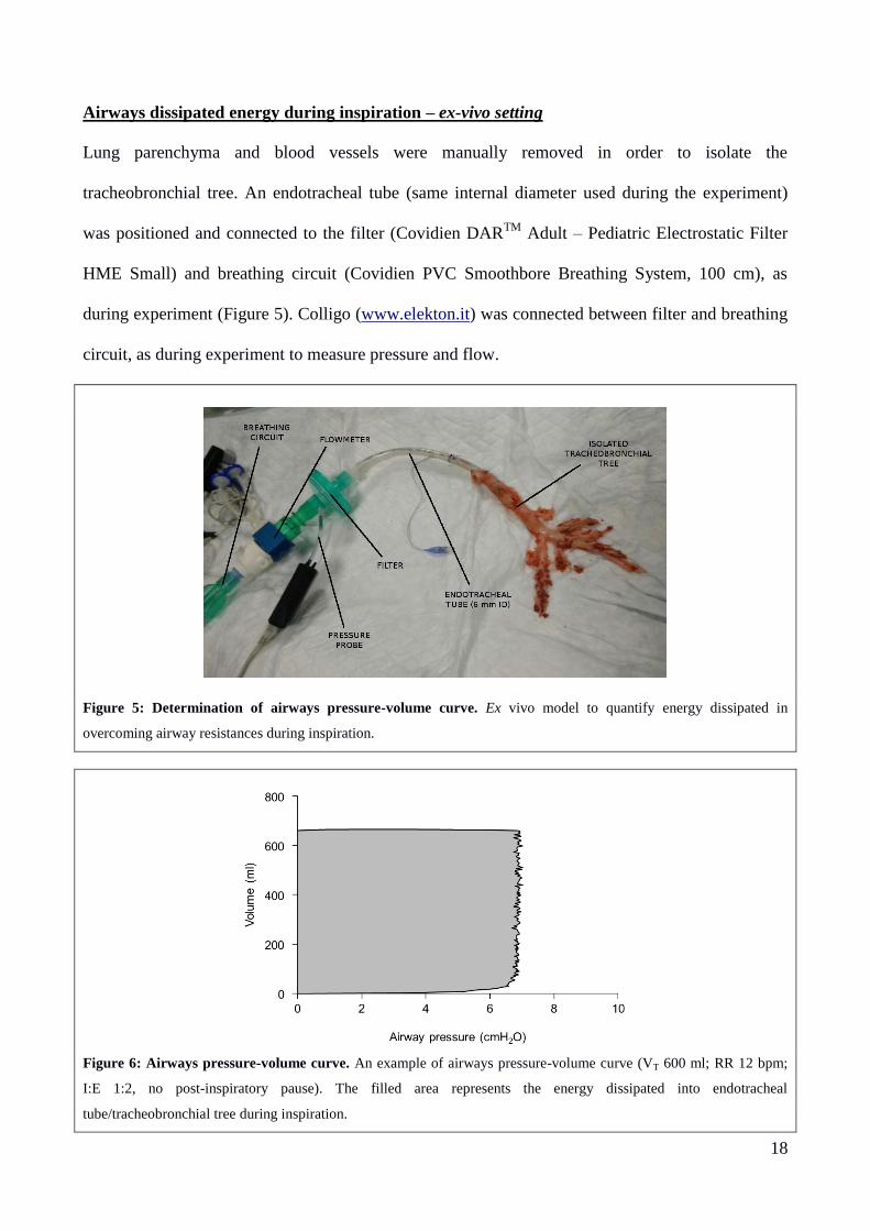
Airways dissipated energy during inspiration – ex-vivo setting

Lung parenchyma and blood vessels were manually removed in order to isolate the

tracheobronchial tree. An endotracheal tube (same internal diameter used during the experiment)

was positioned and connected to the filter (Covidien DARTM

Adult – Pediatric Electrostatic Filter

HME Small) and breathing circuit (Covidien PVC Smoothbore Breathing System, 100 cm), as

during experiment (Figure 5). Colligo (www.elekton.it) was connected between filter and breathing

circuit, as during experiment to measure pressure and flow.

Figure 5: Determination of airways pressure-volume curve. Ex vivo model to quantify energy dissipated in

overcoming airway resistances during inspiration.

Figure 6: Airways pressure-volume curve. An example of airways pressure-volume curve (VT 600 ml; RR 12 bpm;

I:E 1:2, no post-inspiratory pause). The filled area represents the energy dissipated into endotracheal

tube/tracheobronchial tree during inspiration.

http://www.elekton.it/

19


expiration

Energy dissipated in overcoming airway resistances during expiration is function of VT (ml/kg) and

expiratory flow (ml/kg/s). Expiratory flow was computed as average flow:

Expiratory flow (ml/kg/s) = VT (ml/kg) / expiratory time (s)

Actually, expiratory time must be intended as time needed for complete expiration. This does not

necessarily correspond to expiratory time as set on the ventilator (i.e. (60 s / RR) * (1 – I:E)).

Figure 7: Time needed to complete expiration as function of VT. Being expiration a passive process, expiratory time

is only function of VT. Expiratory time (s) = 1.026 + 0.050* VT (ml/kg), r2=0.82, p<0.0001.

Assuming, as an approximation, that airway resistances are similar both during inspiration and

expiration, the effect of expiratory flow on energy dissipation would be similar to that of inspiratory

flow. Therefore, we can derive the energy dissipated into endotracheal tube/tracheobronchial tree

during expiration from the equations of the airways (see Figure 8) considering expiratory flow

instead of inspiratory flow.

Volume (ml/kg)

Expirato

ry T

ime (

s)

10 20 30 40

1.5

2.0

2.5

3.0

20

Energy recoverable at mouth during tidal ventilation

The energy recoverable at mouth during tidal ventilation corresponds to the amount of energy

which is not dissipated into the respiratory system at the end of expiration; this energy,

theoretically, could be recovered at mouth, connecting to the endotracheal tube an appropriate

device to collect energy. This component is specific of our model, and is measurable as the area

between the expiratory limb of the pressure-volume curve and the volume axis (y).

21

Static dissipated energy into the respiratory system

To obtain the static airways pressure-volume curve graph, after pre-oxygenation, inflation and

deflation of the lungs were performed with a supersyringe in steps of 100 ml (last step during

inflation and first step during deflation of 50 ml, if necessary) every ~ 3 seconds. Deflation was

interrupted when resistance was encountered (Figure 8 – dashed curve). Static dissipated energy

into the respiratory system is the hysteresis area of the airways pressure-volume curve.

Figure 8: static and dynamic airways pressure-volume curve. For the same volume (750 ml), dynamic hysteresis

area (solid line), recording during tidal ventilation at respiratory rate 6 breaths/min and I:E = 1:2, is greater that static

hysteresis area (dashed line) because of flow-dependent phenomena (airways dissipation energy and flow dependent

component of dissipated dynamic trans-alveolar energy).

Airway pressure (cmH2O)

Vo

lum

e (

ml)

0 5 10 15 20 25 30 350

200

400

600

800

22

Figure 9: Sequential calculation of dissipated dynamic transalveolar (TA) energy (B), and flow-dependent

component of dissipated dynamic TA energy (C) from the energy delivered to the lung.

We realized this figure subtracting point by point for each piglet:

to obtain Panel B from Panel A, its own energy dissipated in overcoming endotracheal tube/tracheobronchial

resistances + energy recoverable at mouth (matching tidal volume and respiratory rate)

to obtain Panel C from Panel B, its own dissipated static transalveolar energy (matching tidal volume).

Figure 10: relationship between flow dependent component of dissipated dynamic transalveolar energy and

“stress relaxation”. On the x axis we reported the energy resulting from the sequential subtraction previously

described, including the subtraction from the dissipated dynamic transalveolar energy the static component, computed

from the static airways-esophageal pressure-volume curve. On y axis we reported “stress relaxation”, quantified as P1-

P2 (cmH2O) during a 5 seconds end-inspiratory pause on the airways pressure – time graph. As shown, there is a linear

relationship between “stress relaxation” and the flow dependent component of dissipated dynamic transalveolar energy

(r2 = 0.34, p<0.0001): (P1-P2) cmH2O = 3.9 + 17.9 * flow dependent component (J) .

0 10 20 30 40 50 600.0

0.5

1.0

1.5

2.0

2.5

3.0

3.5

05

1015

2025

3035

Volume (ml/kg)

Energ

y D

ELIV

ER

ED

to

the lu

ng

(J)

0 10 20 30 40 50 600.0

0.5

1.0

1.5

2.0

2.5

3.0

3.5

05

1015

2025

3035

Volume (ml/kg)

Tra

ns

alv

eo

lar

dis

sip

ate

dd

yn

am

ice

ne

rgy

(J)

0 10 20 30 40 50 600.0

0.5

1.0

1.5

2.0

2.5

3.0

3.5

05

1015

2025

3035

Volume (ml/kg)

Flo

w-d

ependet

com

ponent

(J)

A B C

ENERGY DISSIPATED IN OVERCOMING

AIRWAYS DURING EXPIRATION

+

ENERGY RECOVERABLE AT MOUTH

DISSIPATED STATIC

TRANSALVEOLAR ENERGY

FLOW –DEPENDENT COMPONENT

OF TRANSALVEOLAR DISSIPATED

DYNAMIC TRANSALVEOLAR ENERGY

TRANSALVEOLAR DISSIPATED

DYNAMIC TRANSALVEOLAR ENERGYENERGY DELIVERED TO THE LUNG

Flow-dependent component (J)

P1

-P2

(cm

H2

O)

0.0 0.1 0.2 0.3 0.4 0.5 0.6

0

5

10

15

23

Figure 11: stress relaxation (P1-P2) as function of delivered transpulmonary energy per breath. Data measured at the

beginning of the study.

Stress relaxation (P1 – P2, cmH2O) = 2.26*( delivered transpulmonary energy per breath, (J)+ 1.73.

Delivered TP energy per Breath (J)

P1-P

2 (

cmH

2O

)

0.5 1.0 1.5

2

3

24

Energy per breath as function of flow and tidal volume

Total delivered energy to the respiratory system

Figure 12: Total delivered energy to the respiratory system at each breath, computed from the dynamic

pressure-volume curves, as function of volume and flow. Total delivered energy, computed on the dynamic pressure-

volume curves, is function of both VT and flow (Panel A). Data points were fit with a two-variables function (i.e. a

surface, shown in Panel B) without intercept and with lower constraint 0, obtaining the following equation (r2=0.92):

(A) Total delivered energy (J) = k1*flow (ml/kg/s)2 + k2* VT (ml/kg)

2 + k3* VT (ml/kg); where:

k1 = 0.0019033

k2 = 0.0005165

k3 = 0.0052903

A

0 10 20 30 40 50 600.0

0.5

1.0

1.5

2.0

2.5

3.0

3.5

05

1015

2025

3035

Volume (ml/kg)

To

tal d

elive

red

en

erg

y to

the

RS

(J)

B

0 10 20 30 40 50 600.0

0.5

1.0

1.5

2.0

2.5

3.0

3.5

05

1015

2025

3035

Volume (ml/kg)T

ota

l de

live

red

en

erg

y to

the

RS

(J)

25

Delivered dynamic transpulmonary energy

Figure 13: delivered dynamic transpulmonary energy at each breath, computed from the dynamic airways-

esophageal pressure-volume curves, as function of volume and flow. Delivered dynamic transpulmonary (TP)

energy, computed on the dynamic pressure-volume curves, is function of both VT and flow (Panel A). Data points were

fit with a two-variables function (i.e. a surface, shown in Panel B) without intercept and with lower constraint 0,

obtaining the following equation (r2=0.87):

(B) Delivered dynamic TP energy (J) = k1*flow (ml/kg/s)2 + k2* VT (ml/kg)

2 + k3* VT (ml/kg); where:

k1 = 0.0017301

k2 = 0.0004441

k3 = 0.0005607

A

0 10 20 30 40 50 600.0

0.5

1.0

1.5

2.0

2.5

3.0

3.5

05

1015

2025

3035

Volume (ml/kg)De

live

red

dyn

am

icT

P e

ne

rgy (J)

B

0 10 20 30 40 50 600.0

0.5

1.0

1.5

2.0

2.5

3.0

3.5

05

1015

2025

3035

Volume (ml/kg)De

live

red

dyn

am

icT

P e

ne

rgy (J)

26


inspiration

Figure 14: Energy dissipated into endotracheal tube/tracheobronchial tree during inspiration. Panel A, energy

dissipated into endotracheal tube/tracheobronchial tree (dissipated AW energy) during inspiration is plotted as function

of flow and VT. Energy (J) dissipated in overcoming airway resistances during inspiration is function of VT (ml/kg) and

inspiratory flow (ml/kg/s). Inspiratory flow was computed as average flow:

- Inspiratory time (s) = (60 s / RR) * I:E

- Inspiratory flow (ml/kg/s) = VT (ml/kg) / inspiratory time (s)

Data points were fit with a two-variables function (i.e. a surface, shown in Panel B) without intercept, obtaining the

following equation (r2=0.88, p<0.0001):

(C) Energy dissipated into endotracheal tube/tracheobronchial tree during inspiration

(J) = k1* flow (ml/kg/s)2 + k2* VT (ml/kg)

2 + k3* flow (ml/kg/s)* VT (ml/kg) + k4* flow (ml/kg/s) + k5* VT (ml/kg);

where:

- k1 = 1.121*10-3

- k2 = -2.754*10-5

- k3 = 2.609*10-4

- k4 = -7.979*10-3

- k5 = 1.947*10-3

- flow = inspiratory flow, as previously computed.

A

0 10 20 30 40 50 60 700.0

0.5

1.0

1.5

2.0

2.5

3.0

3.5

0

10

20

30

40

50

Volume (ml/kg)

Dis

sip

ate

dA

W e

ne

rgy -

insp

ira

tio

n(J

)

B

0 10 20 30 40 50 60 700.0

0.5

1.0

1.5

2.0

2.5

3.0

3.5

0

10

20

30

40

50

Volume (ml/kg)

Dis

sip

ate

dA

We

ne

rgy

-in

sp

ira

tio

n(J

)

27

Energy dissipated in overcoming endotracheal tube/tracheobronchial tree with tube of

diameter of 6 or 8 mm

Figure 15: Airways dissipated energy with endotracheal tubes of different diameter. An endotracheal tube with an

8.0 mm internal diameter (dashed line) dissipates 40-45% energy less than a 6.0 mm tube (solid line). This

measurement was performed on the tracheobronchial tree preparation at the end of the experiment. The figure reports

energy values obtained with a respiratory rate of 15 breaths/min (I:E 1:2).

Volume (ml/kg)

Endotr

acheal tu

be/A

irw

ays

dis

sip

ate

d e

nerg

y (

J)

10 20 30 40 50 60

0.00

0.25

0.50

0.75

1.00

1.25

1.50

1.75

Tube 6.0 mm

Tube 8.0 mm

28

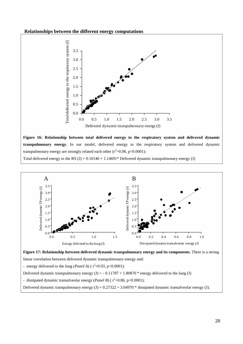
Relationships between the different energy computations

Figure 16: Relationship between total delivered energy to the respiratory system and delivered dynamic

transpulmonary energy. In our model, delivered energy to the respiratory system and delivered dynamic

transpulmonary energy are strongly related each other (r2=0.98, p<0.0001):

Total delivered energy to the RS (J) = 0.10146 + 1.14691* Delivered dynamic transpulmonary energy (J)

Figure 17: Relationship between delivered dynamic transpulmonary energy and its components. There is a strong

linear correlation between delivered dynamic transpulmonary energy and:

- energy delivered to the lung (Panel A) ( r2=0.93, p<0.0001):

Delivered dynamic transpulmonary energy (J) = - 0.11787 + 1.80870 * energy delivered to the lung (J)

- dissipated dynamic transalveolar energy (Panel B) ( r2=0.86, p<0.0001):

Delivered dynamic transpulmonary energy (J) = 0.27322 + 3.04970 * dissipated dynamic transalveolar energy (J).

Delivered dynamic transpulmonary energy (J)

To

tal d

eliv

ere

den

erg

y t

oth

e r

esp

ira

tory

syst

em

(J)

0.0 0.5 1.0 1.5 2.0 2.5 3.0 3.5

0.0

0.5

1.0

1.5

2.0

2.5

3.0

3.5

Dissipated dynamictransalveolar energy (J)

Deli

vere

dd

ynam

icT

P e

nerg

y (

J)

0.0 0.2 0.4 0.6 0.8 1.00.0

0.5

1.0

1.5

2.0

2.5

3.0

3.5

Energy delivered to the lung (J)

Del

iver

ed d

ynam

ic T

P e

ner

gy (

J)

0.0 0.5 1.0 1.50.0

0.5

1.0

1.5

2.0

2.5

3.0

3.5

A B

29

Supplementary data from the main experiments

Equations of linear regressions in Table 1 e Table 2 (main text)

In this paragraph we reported equations of linear regressions presented in Table 1 (main text)

(Figure 18).

Weight (kg) = 21.57 – 0.09 * respiratory rate (breaths/min) r2 = 0.05, p=0.44

Tidal volume (ml) = 796.67 + 0 * respiratory rate (breaths/min) r2 = 0.00, p=1.00

Tidal volume (ml/kg) = 36.90 + 0.17 * respiratory rate (breaths/min) r2 = 0.09, p=0.27

Strain = 3.58 – 0.04 * respiratory rate (breaths/min) r2 = 0.02, p=0.64

Tidal volume/lung tissue (ml/g) = 1.91 + 0.01 * respiratory rate (breaths/min) r2 = 0.05,

p=0.48

Peak pressure (cmH2O) = 26.50 + 0.89 * respiratory rate (breaths/min) r2 = 0.74, p<0.0001

Plateau pressure (cmH2O) = 23.13 + 0.19 * respiratory rate (breaths/min) r2 = 0.21, p=0.09

Transpulmonary pressure (cmH2O) = 16.59 + 0.14* respiratory rate (breaths/min) r2 = 0.06,

p=0.39

PaO2/FiO2 = 505.53 + 0.44 * respiratory rate (breaths/min) r2 = 0.00, p=0.90

pH = 7.33 + 0.03 * respiratory rate (breaths/min) r2 = 0.64, p<0.001

PaCO2 (mmHg) = 55.10 – 2.97 * respiratory rate (breaths/min) r2 = 0.61, p<0.001

Respiratory system elastance (l/cmH2O) = 32.75 + 0.03 * respiratory rate (breaths/min) r2 =

0.00, p=0.95

Lung elastance (l/cmH2O) = 23.04 + 0.15 * respiratory rate (breaths/min) r2 = 0.01, p=0.67

Chest wall elastance (l/cmH2O) = 9.71 – 0.12 * respiratory rate (breaths/min) r2 = 0.02,

p=0.60

30

Mean arterial pressure (mmHg) = 103.67 – 0.89 * respiratory rate (breaths/min) r2 = 0.04,

p=0.47

Heart rate (beats/min) = 95.23 + 2.19 * respiratory rate (breaths/min) r2 = 0.10, p=0.25

Total lung volume (ml) = 605.29 + 7.61 * respiratory rate (breaths/min) r2 = 0.06, p=0.43

Total lung tissue (g) = 415.19 – 2.49 * respiratory rate (breaths/min) r2 = 0.09, p=0.31

Well inflated tissue (%) = 0.04 + 0.02 * respiratory rate (breaths/min) r2 = 0.16, p=0.17

Poorly inflated tissue (%) = 0.87 – 0.02 * respiratory rate (breaths/min) r2 = 0.21, p=0.11

Not inflated tissue (%) = 0.09 – 0.00 * respiratory rate (breaths/min) r2 = 0.00, p=0.96

Lung inhomogeneity extent (%) = 7.95 + 0.01 * respiratory rate (breaths/min) r2 = 0.00,

p=0.94

In this paragraph we reported equations of linear regressions presented in Table 2 (main text)

(Figure 18).

Delivered dynamic transpulmonary energy (per breath) (J)= 0.70 + 0.05 * respiratory rate

(breaths/min) r2 = 0.35, p=0.02

Average inspiratory flow (l/s) = 8.84 + 36.53 * respiratory rate (breaths/min) r2 = 0.93,

p<0.0001

Delivered dynamic transpulmonary energy load (J/min) = -2.69 + 1.51 * respiratory rate

(breaths/min) r2 = 0.90, p<0.0001

31

Respiratory rate (breaths/min)

4 6 8 10 12 14

0.6

0.8

1.0

1.2

1.4

1.6

1.8


Avara

ge

inspirato

ry f

low

(l/s)

4 6 8 10 12 14

0.1

0.2

0.3

0.4

0.5

0.6


Deliv

ere

ddynam

ic

tran

sp

ulm

ona

ry e

ne

rgy loa

d(J

/min

)

4 6 8 10 12 14

5

10

15

20


weig

ht

(Kg)

4 6 8 10 12 14

19

20

21

22

23


Tid

al vo

lum

e (m

l)

4 6 8 10 12 14

700

750

800

850

900

950


Tid

alvolu

me (m

l/K

g)

4 6 8 10 12 14

34

36

38

40

42


Str

ain

4 6 8 10 12 14

2

3

4

5

6


Tid

al volu

me/lung tis

sue (m

l/g)

4 6 8 10 12 14

1.6

1.8

2.0

2.2

2.4


Pea

k p

ressu

re (

cm

H2

O)

4 6 8 10 12 14

30

35

40


Pla

teau p

ressure

(cm

H2O

)

4 6 8 10 12 14

21

22

23

24

25

26

27

De

live

red

dy

na

mic

TP

en

erg

y (

J)

32

Respiratory rate (breaths/min)Tra

ns

pu

lmo

na

ry p

res

su

re (

cm

H2

O)

4 6 8 10 12 14

14

16

18

20

22


PaO

2/F

iO2

4 6 8 10 12 14

400

450

500

550

600


pH

4 6 8 10 12 14

7.3

7.4

7.5

7.6

7.7

7.8

Respiratory rate (breaths/min)P

aC

O2

(m

mH

g)

4 6 8 10 12 14

10

20

30

40

50

60


Re

sp

irato

ry s

yste

m e

lasta

nce

(l/cm

H2

O)

4 6 8 10 12 14

25

30

35

40

45


Lun

g e

lasta

nce

(l/cm

H2O

)

4 6 8 10 12 14

15

20

25

30


Ch

est w

all

ela

sta

nce

(l/cm

H2

O)

4 6 8 10 12 14

4

6

8

10

12

14


Me

an

art

eria

l p

ressu

re (

mm

Hg

)

4 6 8 10 12 14

70

80

90

100

110

120


He

art

rate

(be

ats

/min

)

4 6 8 10 12 14

60

80

100

120

140

160

180


To

tal l

un

g v

olu

me

(m

l)

4 6 8 10 12 14

500

600

700

800

900

33

Figure 18: Linear regressions for Table 1 and Table 2 (main text)


Tota

l lung t

issue (

g)

4 6 8 10 12 14

360

380

400

420

440

460


No

tin

fla

ted tis

sue

(%

)

4 6 8 10 12 14

5

10

15

20

25


Poo

rly

infl

ate

d t

issue (

%)

4 6 8 10 12 14

20304050607080

90


We

ll in

fla

ted

tis

su

e (%

)

4 6 8 10 12 14

0

20

40

60


4 6 8 10 12 14

4

6

8

10

Inh

om

og

en

eit

ye

xte

nt

(%)

34

Regressions for Figure 4 (main text)

Figure 19: Regressions for Figure 4 (main text). Regressions on the entire pool of data to realize figure 4 (main text).

Panel A: ∆ delivered dynamic transpulmonary energy (J) = 0.09 + 0.03*∆ intratidal opening and closing (%), r2=0.23,

p<0.0001. Panel B: ∆ delivered dynamic transpulmonary energy (J) = 0.23 + 0.24*∆ strain, r2=0.14, p<0.0001. Panel C:

∆ delivered dynamic transpulmonary energy (J) = 0.08 + 0.04*∆ lung inhomogeneity extent (%), r2=0.37, p<0.0001.

A

∆ Intratidal opening and closing %

-10 0 10 20

-0.5

0.0

0.5

1.0

1.5

∆ D

eliv

ere

dT

P e

ne

rgy p

er

bre

ath

(J)

B

∆ Strain

-1.0 -0.5 0.0 0.5 1.0 1.5 2.0

-0.5

0.0

0.5

1.0

1.5

C

∆ Inhomogeneity extent %

-5 0 5 10 15 20 25

-0.5

0.0

0.5

1.0

1.5

35

Thresholds calculation

In order to analyze our results, we calculated 3 thresholds of energy load to VILI development

(defined as an increase of at least 10% of the lung weight at last CT scan) (Figure 20):

The first one on total delivered energy load to the respiratory system: 16.7 J/min

The second one on delivered dynamic transpulmonary energy load: 12.1 J/min

The third one on delivered energy load to the lung: 6.9 J/min

Figure 20. ROC analysis for thresholds calculation. Panel A: threshold for total delivered energy load to the

respiratory system for VILI development 16.7 J/min, Specificity 100%, Sensibility 100%. Panel B: threshold for

delivered dynamic transpulmonary energy load for VILI development 12.1 J/min, Specificity 100%, Sensibility 100%.

Panel C: threshold for delivered energy load to the lung for VILI development 6.9 J/min, Specificity 86%, Sensibility

67%.

A

False positive rate

Tru

ep

ositiv

e rate

0.0 0.2 0.4 0.6 0.8 1.0

0.0

0.2

0.4

0.6

0.8

1.0

38.5

14

19.6

25.1

30.6

B

False positive rate

Tru

ep

ositiv

e rate

0.0 0.2 0.4 0.6 0.8 1.0

0.0

0.2

0.4

0.6

0.8

1.0

26.5

11

15.5

19.9

24.4

C

False positive rate

Tru

ep

ositiv

e rate

0.0 0.2 0.4 0.6 0.8 1.0

0.0

0.2

0.4

0.6

0.8

1.0

1.9

3.5

5.2

6.8

8.5

10.1

36

Estimation of delivered dynamic transpulmonary energy load threshold on tidal volume

delivered at respiratory rate of 15 breaths/minute

Previously published data suggest that, in healthy piglets, ventilator-induced lung damage

develops at 54 hours only when a strain greater than 1.5-2 is reached or overcome at a respiratory

rate of 15 breaths/min.1 We estimated the delivered dynamic transpulmonary energy load

corresponding to this “threshold” from the 6 piglets’ equations.

In our 6 piglets, average functional residual capacity was 246 ml and average weight 18.5

Kg. A strain of 1.5 corresponded to a delivered dynamic transpulmonary energy per breath of 0.57

J, corresponding to a delivered dynamic transpulmonary energy load of 8.6 J/min. A strain of 2

corresponded to a delivered dynamic transpulmonary energy per breath of 1.02 J, corresponding to

a delivered dynamic transpulmonary energy load of 15.3 J/min.

37

Table 1. Clinical variables at the end of the study in piglets ventilated with a delivered

dynamic transpulmonary energy load per minute below and above lethal threshold

< 12.1 J/min

n=9 ≥ 12.1 J/min

n=6 P-value

Weight (kg) 21±2 20±2 0.47

VT

(ml) 783±67 817±88 0.46

(ml/kg) 37±2 40±1 0.02

Strain (VT/FRC) 2.99±0.59 10±8.41 0.23

VT/tissue (ml/g) 2.03±0.3 1.41±0.43 0.02

Study duration (hour) 56.2±5.5 29.4±14.2 <0.01

Peak pressure (cmH2O) 40±10 63±12 <0.01

Plateau pressure (cmH2O) 26±7 41±12 0.18

Transpulmonary pressure (cmH2O) 18±5 29±6 <0.01

PaO2/FiO2 470±77 282±182 0.09

pH 7.45±0.09 7.39±0.18 0.53

PaCO2 (mmHg) 36.2±21.9 18.0±8.6 0.15

Respiratory System Elastance (cmH2O/l) 32±11 42±12 0.18

Lung Elastance (cmH2O/l) 25±10 39±10 0.02

Chest Wall Elastance (cmH2O/l) 7±4 5±5 0.52

Mean Arterial Pressure (mmHg) 88±9 67±26 0.04

Heart Rate (bpm) 83±21 118±38 0.11

Lactates (mEq/l) 0.6±0.3 3.4±3.8 0.10

SvO2 (%) 70±12 50±10 0.01

Fluid balance (ml) -897±1284 1441±1233 0.01

Total lung volume (ml) 658±46 810±153 0.10

Total lung tissue (g) 387±31 614±152 <0.01

Well inflated tissue (%) 27±17 14±21 0.10

Poorly inflated tissue (%) 61±14 35±21 0.02

Not-inflated tissue (%) 12±8 51±36 0.07

Recruitment (%) 6±6 39±31 0.05

Inhomogeneity extent (%) 10±3 14±9 0.94

Autoptic lung weight (g) 313±165 496±125 0.02

Wet to dry ratio 5.7±1.4 6.9±1.1 0.18

Data are presented as mean ± standard deviation. The two groups were compared with two-tailed Wilcoxon Signed-

Ranks Test. CT scan was not available in two piglets (both ventilated with a delivered dynamic transpulmonary energy

38

load per minute <16.7 J/min), so CT scan data were computed on 13 piglets. Fluid balance does not include drugs. Wet

to dry ratio was computed in 11 piglets (respectively 6 and 5 in groups ventilated with low and high energy load).

Table 2. Energy load at the end of the study in piglets ventilated with delivered dynamic

transpulmonary energy load below and above the threshold

< 12.1 J/min

n=9 ≥ 12.1 J/min

n=6 P-value

Delivered dynamic TP energy per breath (J)

1.2±0.3 2.5±0.3 <0.001

Average Inspiratory Flow (l/s) 0.25±0.11 0.50±0.10 <0.001

Delivered dynamic TP energy per minute (J/min)

7.6±4.2 33.5±7.7 <0.001

Data are presented as mean ± standard deviation. The two groups were compared with two-tailed Wilcoxon Signed-

Ranks Test.

39

Figure 21: Relationships between increase of stress relaxation (P1-P2 cmH2O) and VILI

development

Delta stress relaxation (P1-P2) (cmH2O)

Delta P

aO

2/F

iO2

0 2 4 6 8 10

-400

-300

-200

-100

0

100

r2

= 0.29, P=<0.01, intercept = -21.84, slope = -24.44

Delta stress relaxation (P1-P2) (cmH2O)

Delta lung w

eig

ht

(g)

0 2 4 6 8 10

-100

0

100

200

300

400

500r2

= 0.44, P=<0.001, intercept = 6.46, slope = 31.47

Delta stress relaxation (P1-P2) (cmH2O)in

hom

ogeneity e

xte

nt

(% o

f lu

ng v

olu

me)

0 2 4 6 8 10

-5

0

5

10

15

20

25

r2

= 0.39, P=<0.01, intercept = 0.99, slope = 1.32

Relationships between increase of stress relaxation (P1-P2 cmH2O) and VILI development

40

Histology

Histological analysis was available in 13 piglets: 9 from the main experiments (3 ventilated at 15

breaths/min, 2 ventilated at 12 breaths/min, 1 ventilated at 9 breaths/min and 3 ventilated at 6

breaths/min) and 4 from the confirmatory experiments (RR 35 breaths/min). For each of the

histological parameters considered we computed a median value in each piglet (8 samples/piglet)

(Table 7 and Figure 22).

Table 7: Histology

No ventilator-induced

lung edema (6 piglets)

Ventilator induced lung

edema (7 piglets)

P-value

Hyaline membranes 0.69 [0.53-0.84] 1.75 [1.28-1.76] 0.03

Ruptured alveoli 0.50 [0.36-0.59] 0.37 [0.11-0.81] 0.89

Interstitial infiltrate 1.94 [1.31-2.09] 1.75 [1.61-2.19] 0.89

Infiltrate intensity 1.60 [1.30-1.75] 1.50 [1.41-1.56] 1.00

Intra-alveolar infiltrate 0.00 [0.00-0.19] 0.50 [0.34-0.77] 0.08

Red blood cells leakage 1.50 [1.22-1.88] 1.00 [0.81-1.00] 0.01

Piglets were divided according to the presence/absence of ventilator-induced lung edema. Data are presented as median

[interquartile range] and compared with Wilcoxon test.

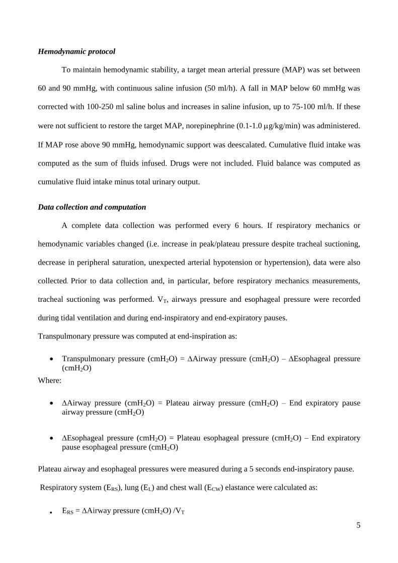
Figure 22: Photomicrographs of lung sections stained with haematoxylin-eosin showing the effect of delivered

dynamic energy load below (A) and above (B, C) the threshold. At high delivered dynamic energy load lung injury

is evident and characterized by hyaline membranes, capillary congestion and hemorrhaging, inter- and intra-alveolar

infiltratum containing red and white blood cells, alveoli thickening and collapse, deposition of basophilic material on

alveoli walls, leading to lung structure disruption. Original magnification: 10x.

Supplemental references

A B C

41

1. Protti A, Cressoni M, Santini A, Langer T, Mietto C, Febres D, Chierichetti M, Coppola S, Conte

G, Gatti S, Leopardi O, Masson S, Lombardi L, Lazzerini M, Rampoldi E, Cadringher P,

Gattinoni L: Lung stress and strain during mechanical ventilation: any safe threshold? Am J

Respir Crit Care Med 2011; 183:1354–62

2. Cressoni M, Chiurazzi C, Gotti M, Amini M, Brioni M, Algieri I, Cammaroto A, Rovati C,

Massari D, Castiglione CB di, Nikolla K, Montaruli C, Lazzerini M, Dondossola D, Colombo A,

Gatti S, Valerio V, Gagliano N, Carlesso E, Gattinoni L: Lung Inhomogeneities and Time Course

of Ventilator-induced Mechanical Injuries. Anesthesiology

2015doi:10.1097/ALN.0000000000000727

3. Weibel ER, Sapoval B, Filoche M: Design of peripheral airways for efficient gas exchange.

Respir. Physiol. Neurobiol. 2005; 148:3–21

4. Cressoni M, Cadringher P, Chiurazzi C, Amini M, Gallazzi E, Marino A, Brioni M, Carlesso E,

Chiumello D, Quintel M, Bugedo G, Gattinoni L: Lung inhomogeneity in patients with acute

respiratory distress syndrome. Am. J. Respir. Crit. Care Med. 2014; 189:149–58

Supplemental Digital Content 1 Mechanical power and the...

Documents

Transcript of Supplemental Digital Content 1 Mechanical power and the...