Suburban Travel Patterns in Burglary

Suburban Travel Patterns in Burglary

Research Report

John Fernandez Joe Clare

Frank Morgan

Crime Research Centre

University of Western Australia

Prepared for the Office of Crime Prevention,

Department of Premier and Cabinet Western Australia

May 2006

i

TABLE OF CONTENTS

PREFACE .................................................................................................................... iii

EXECUTIVE SUMMARY........................................................................................ iv

INTRODUCTION.......................................................................................................1

RESEARCH STRUCTURE........................................................................................2

CHAPTER 1: Distance To Burglary.........................................................................4

Burglary Type.....................................................................................................5

Offender Characteristics ..........................................................................6

Distance Decay ..........................................................................................8

Distances Travelled To and From Suburbs .........................................15

CHAPTER 2: Area by Area Analysis.....................................................................18

District-level Analysis ....................................................................................19

Subdistrict-level Analysis ......................................................................20

Central Metropolitan district................................................................20

East Metropolitan district .....................................................................22

North West Metropolitan district .........................................................24

South East Metropolitan district ..........................................................26

South Metropolitan district ..................................................................28

West Metropolitan district....................................................................30

Suburb-level Analysis for Selected Suburbs.............................................32

CHAPTER 3: Offender Interview Questions ......................................................34

General ..............................................................................................................35

What type of place was burgled?...........................................................35

Had you, or anyone you knew, broken into this place before? ..............36

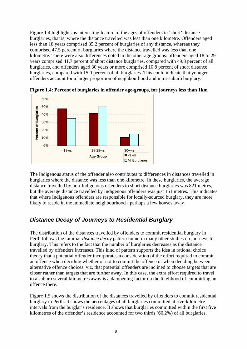
Did you have information about this place before?...............................37

What time of day? .................................................................................38

Why were you in the area?....................................................................39

How did you get to the burglary? .........................................................40

Did you leave the place in the same way that you got there? ...............41

ii

Where did you go after the break-in? ....................................................42

What was taken from the break-in?(Portability) ..................................43

Distance Analysis ............................................................................................44

Distance from home...............................................................................44

Distance from place slept night before ..................................................45

Distance, by mode of transport to burglary ..........................................45

Storage distance from the break-in........................................................46

Distance, by portability of items taken..................................................46

Distance from home, by time of day ......................................................47

Distance from home, by drug use..........................................................47

REFERENCES ............................................................................................................48

APPENDIX A: Caveats on WA Police Data .........................................................49

iii

PREFACE Western Australia has among the highest rates of domestic burglary of any State or Territory in Australia, despite recent encouraging developments. Hence, the reduction of burglary is a priority area for crime prevention in Western Australia. The major goal of this research is to uncover both city-wide and localised issues in offenders’ travel patterns in committing burglary in Perth, with a view to informing crime prevention policy development aimed at reducing the rate of burglary. The research explores patterns in burglary offences with respect to journey to crime in Perth, Western Australia. It includes analyses of distance travelled, offender and suburb characteristics, as well as disposal patterns. Existing burglary reduction and prevention programs offer local knowledge about specific areas and endemic issues. However, this research utilises systematically recorded data about recorded burglaries. Such data, as well as the offender survey information, are of utmost importance and provide compelling motivation for analysis. The research adds to our existing knowledge of burglary and its reduction, in terms of both ‘in the field’ knowledge and in the more formal body of crime prevention literature. The survey of offenders provides invaluable insight into the practical issues and patterns in offenders’ choice of target, disposal routes and methods, and how these relate to offender characteristics, including place of residence. It is hoped that the results presented here will provide existing, and indeed future, programs with reliable knowledge about local patterns – in some contexts confirming local knowledge, and in other contexts challenging and extending that knowledge. The results are intended to be used to inform crime prevention policy, aid crime prevention practitioners and to contribute to criminological theory. This will provide the State with previously unavailable empirical knowledge about offender movements and characteristics, victimisation characteristics, and suburb-by-suburb travel patterns. The research was undertaken by John Fernandez, Frank Morgan and Joe Clare of the Crime Research Centre, University of Western Australia. The authors thank and acknowledge the advice and expertise of Professor Pat Brantingham and Professor Paul Brantingham from Simon Fraser University, British Columbia, Canada. The research was funded by the Office of Crime Prevention.

iv

EXECUTIVE SUMMARY This Executive Summary is designed to highlight important results from each of the four distinct stages of the project. Each of these results is presented as a short ‘grab point’ that can be taken and used as a separate item. However, some results may reveal other important issues when considered together with other results. 1. Distance to Burglary

1.1. Burglaries committed within the first five kilometres of the offender’s residence accounted for two thirds (66.2%) of all burglaries and about half (47.8%) of all burglaries were committed within two kilometres of the offender’s residence.

1.2. About one third (34.9%) of all burglaries were committed within one kilometre of the offender’s residence and about one in seven (13.9%) were committed within 200 metres. This indicates the local nature of burglary, and it is likely that at least half of all burglaries are committed within the offender’s own residential suburb or an adjacent suburb.

1.3. Overall, the average distance to burglary (all types) in Perth was 6.1km. The average distance for residential burglary in Perth was 5.9km, which was less than for commercial burglary (7.1km), but greater than for burglary on other types of premises (5.4km).

1.4. Consideration of points 1 to 3, above, together suggest that even though most burglaries are committed relatively close to the offender’s home, there are also many longer journeys taken by burglars. Care should be taken here: it should not be assumed, since the average distance to residential burglary is 5.9km, that most burglaries are committed within this distance. The vast suburban sprawl of the Perth metropolitan area ensures that this average distance will be inflated, compared with the median distance of about two kilometres.

1.5. Females have a smaller proportion of their offences (30.5%) less than two kilometres from their place of residence, compared with male offenders (50.2%). The average distance travelled to residential burglary for males was 5.6km, which is less than for females (8.2km).

1.6. For offenders under 18 years of age the average distance travelled was 3.9km, which is much less than the average distance travelled for offenders aged between 18 and 29 years (7.1km) and for offenders ages 30 years and older (6.5km).

1.7. Juvenile males travel considerably less (on average) than juvenile females (i.e., 3.4km, compared with 8.4km). For juvenile males, the proportion of burglaries committed within two kilometres of their residence was 65.3 percent and for juvenile females was 32.4 percent.

1.8. Offenders aged less than 18 years comprised 35.2 percent of burglaries of any distance, whereas they comprised 47.5 percent of burglaries where the distance travelled was less than one kilometre.

1.9. Indigenous and non-Indigenous offenders have roughly the same proportions of their offences committed within two kilometres of their residence. However, non-Indigenous juveniles commit 70.2 percent of their offences within two kilometres of their home, compared with Indigenous juveniles (45.3%).

v

1.10. For Indigenous offenders, the average distance travelled was 6.6km, which is slightly greater than for non-Indigenous offenders (5.8km).

1.11. Where Indigenous offenders are responsible for locally-sourced burglary, they are more likely to reside in the immediate neighbourhood – perhaps just a few houses away.

1.12. For burglaries within the first 200 metres of the offender’s home, Indigenous offenders accounted for larger proportions of the burglaries than non-Indigenous offenders.

1.13. When the distribution of distances travelled was examined at 100-metre intervals, it was found that there was no ‘home buffer’ effect - a significant proportion of burglaries are committed by residents in the neighbourhood.

1.14. There is some evidence for a home-buffer effect for juvenile offenders, whereby they tended to avoid offending very close to their place of residence. Juveniles accounted for a smaller proportion of burglaries that occurred within the first 100 metres of their home, even though they accounted for larger proportions of burglaries between 200 to 700 metres away from the their home.

1.15. There was found to be a pattern of increasing distances travelled as the income of the target suburb increased. Thus, the income level of the target suburb was having a influence on how far offenders will travel to commit burglary. This confirms a rational choice argument that the potential for greater rewards may be motivation for exerting greater effort (i.e., travelling further).

1.16. Distances travelled during the day (6am to 6pm) were compared with distances travelled at night (6pm to 6am). There was no significant difference between the distance decay patterns of burglaries occurring during the day and those occurring during the night. This indicates that the pattern of distances travelled by offenders is not influenced by day or night. Even though most burglaries occur during the day, crime prevention interventions aimed at preventing locally sourced offending, should not ‘turn off’ at night, but need to be in place both during the day and the night.

2. Stage Two: Area by Area Analysis

2.1. Of all the metropolitan police districts, the Central Metropolitan district had the lowest proportion of its offences committed by local (resident) offenders (30.5%).

2.2. Of all the metropolitan police districts, the South Metropolitan district had the highest proportion of its offences committed by local (resident) offenders (87.4%).

2.3. Of all the metropolitan police districts, the West Metropolitan district had the lowest proportion of its locally-resident offenders committing burglaries within its own district (53.4%).

2.4. Of all the metropolitan police districts, the South Metropolitan district had the highest proportion of its locally-resident offenders committing burglaries within its own district (85.7%).

2.5. For all offences in the metropolitan area, about two thirds (68.4%) were committed in three of the six districts (South East Metropolitan, 25.9%, South Metropolitan, 21.2% and West Metropolitan, 21.3%).

2.6. Of all offences in the metropolitan area, 4.5 percent occurred in the Central Metropolitan district; however, 9.9 percent of all offenders in the metropolitan area resided in the Central Metropolitan district.

2.7. Of all offences in the metropolitan area, 21.3 percent occurred in the West Metropolitan district; however, only 16.7 percent of all offenders in the metropolitan area resided in the West Metropolitan district.

vi

2.8. Of all offences in the South East Metropolitan district, 37.7 percent were committed by offenders from the Gosnells subdistrict. This is the highest offender contribution to its district offences of any subdistrict across the metropolitan area.

2.9. Of all offenders living in the South East Metropolitan district, 37.0 percent committed their offences in the Gosnells subdistrict. This is the highest offence concentration from its district offenders in any subdistrict across the metropolitan area.

3. Stage Three: Offender Interview Questions

3.1. Older offenders were more likely to burgle places selling alcohol than were younger offenders, while younger offenders were more likely to burgle shops than were older offenders.

3.2. Indigenous offenders were more likely than non-Indigenous offenders to burgle houses instead of other premises.

3.3. The night-time (12am-6am) accounted for almost a third (32.1%) of burglaries. 3.4. Almost half of the offenders (46.9%) were in the area specifically to do a break-in. 3.5. Indigenous offenders were less likely to be in the area to do a break-in than were

non-Indigenous offenders. 3.6. Travelling by car and on foot each accounted for approximately 45 percent of the

burglaries. 3.7. Of the 109 offenders that used a car, almost one third (32.1%) of them used a

stolen car. This means that about one in seven burglaries involved a stolen car. 3.8. Indigenous offenders were much more likely to walk to a burglary than were non-

Indigenous offenders. 3.9. Most offenders (83.1%) used the same mode of transport to leave the break-in as

they used to travel to the break-in. 3.10. Almost 30 percent of burglars went home after the burglary, 23.9 percent went to a

friend’s house and 15.6 percent went to a dealer, fence or pawnbroker. Only 2.5 percent went to do another break-in and only 3.7 percent got caught.

3.11. About two thirds of burglaries involved taking only smaller, portable items. 3.12. Offenders who took large items were more likely to use a car and offenders who

took only small items were more likely to walk. 3.13. 62.6 percent of the burglaries were more than three kilometres away and 15.2

percent were within one kilometre. 3.14. Older offenders were more likely to travel larger distances than were younger

offenders. Indigenous offenders were more likely to travel shorter distances than were non-Indigenous offenders.

3.15. When the offender walked, just over 30 percent of the burglaries were less than one kilometre away, but almost 40 percent were more than three kilometres away.

3.16. Almost two thirds of offenders stored the stolen items more than three kilometres away.

3.17. Portability of stolen items did not show a marked effect on the distance travelled. 3.18. During the morning period distances of less than one kilometre make up a larger

proportion of the burglaries than they do in other time periods, and during the night-time period they make up a smaller proportion.

3.19. Burglars with no frequent and/or no severe drug use travel less distances to burgle than do burglars with frequent and/or severe drug use.

vii

4. Stage Four: Residential Burglary Target Suburb Selection 4.1. Variables included in the models were based on rational choice theory and were

grouped by rewards, risk or effort. 4.2. Target suburb affluence was found to be predictive of burglary victimisation, with

an increase in estimated weekly income increasing the odds of victimisation by a factor of 1.06.

4.3. The odds of burglary victimisation decreased by a factor of 0.83 for every kilometre increase between the burglar’s home suburb and the target suburb.

4.4. The percentage of rental properties in the target suburb increased the odds of victimisation by a factor of 1.26 for every 10 per cent increase in rental properties.

4.5. An increase in ethnic heterogeneity increased the odds of burglary victimisation by a factor of 2.16.

4.6. All offenders were more likely to target suburbs as the percentage of Aboriginal people in the suburb increased.

4.7. For Aboriginal offenders, the odds of offending increased by a factor of 7.23 as the percentage of Aboriginal people in the suburb increased by 10 per cent.

4.8. If there was a train station adjacent to both the offender and the target suburbs, then the odds of offending increased by a factor of 2.44.

4.9. If there was a major river dividing the offender and the target suburbs, then the odds of offending decreased by about a third.

4.10. If there was a major highway dividing the offender and the target suburbs, then the odds of offending decreased by about 60 percent.

4.11. The discrete spatial choice approach to target suburb selection provided scope for analysis of the relationship between target characteristics, such as average weekly household income, and offender demographics, such as age.

4.12. The approach outperformed the capacity of previous attempts to model criminal location choice.

1

INTRODUCTION The incidence of burglary is not evenly distributed and the patterns in offending and victimisation vary among areas, with burglary rates varying widely across metropolitan Perth. These patterns depend on a general opportunity structure for domestic and commercial burglary, influenced by factors including the following:

• the proximity of burglary targets to offender residence; • the attractiveness of targets; • the routine activities of potential offenders and likely offenders; • methods of disposal of stolen goods.

An important aspect of this is our understanding of offenders’ journey to crime; that is, the travel movements offenders choose to take to commit their offence, as well as the journey they take immediately after the burglary. The importance of this is highlighted by questions that are frequently asked about the patterns of offender movements, such as:

• How far do burglars travel to offend? • Which suburbs do offenders come from and which suburbs do they offend in? • How much burglary is committed by non-local offenders? • Which areas are more at risk of intra-suburb offending? • What are the areas that should be targeted for particular interventions? • What transport modes and routes do offenders take to commit burglaries? • How do offenders dispose of the stolen goods? • Does the travel distance vary for offenders of different socio-demographic profiles or

for different areas? • How do offender characteristics affect the level of local offending?

The answers to these types of questions are necessary for implementing timely interventions aimed at particular areas at risk. More formally, however, there is a glaring lack of research on the journeys to and from burglary in Australia, and this project goes some way to filling that void. Furthermore, the already existing research was conducted almost entirely overseas, and was applicable to areas that may not have the same social, economic and cultural conditions as Australia, or indeed Perth. For example, much of the empirical base underpinning predictions of journey to burglary patterns assumes a British or East Coast American high density urban framework, which is clearly in contrast with Perth’s low density sub-urban structure. The Perth results are of great interest empirically and theoretically in comparison with published studies in North America and Europe, as well in direct contemporary comparison with a sister study in Vancouver. Routine activities theory (Cohen and Felson, 1979) and pattern theory (Pat and Paul Brantingham, 1984) would predict that most burglaries are committed by locals, but these predictions are based on British or East Coast American urban structures and neighbourhood patterns. So, Sydney, and to some extent Melbourne, would also fit this pattern. But low density cities, such as Perth, keyed to longer automobile commutes rather than public transit have different neighbouring patterns and different patterns of neighbourhood knowledge that are much more strung out across the face of the city. In low density suburbanised cities people live their lives in networks of family, friends and work acquaintances that are spread

2

out across the face of the city. There are some hints of this in the Home Office journey to burglary study, “The Road to Nowhere” (Wiles and Costello, 2000), and there are stronger hints in the geographic pattern exhibited in the West Midlands Police FFLINTS police information system. In such cities burglars become neighbourhood insiders and have many more local starting places (besides home) because of the way life is lived in low density cities. In the context of local crime prevention in Western Australia, the research has relevant and practical implementation capacity. A starting point here would seem to be the (big) assumption that burglary is committed almost entirely by strangers. Schemes such as Neighbourhood Watch assume that watching activities will be easily able to identify those who are strangers to the area. However, this study throws more light on this issue. It provides a suburb by suburb analysis of the nature of burglary, with respect to offender characteristics and travel patterns, so that interventions can be tailor-made to the crime patterns found for individual Perth suburbs. Offenders’ choice of target and disposal behaviour is put into the context of local Perth suburbs.

RESEARCH STRUCTURE The project examined the journey to burglary for suburbs and police sub-districts in metropolitan Perth from two perspectives – as locations of victims and as locations of offenders. It examines the journey to burglary as recorded in police records of burglary and ‘processed persons’. It also includes a survey of offenders, in which offenders were questioned about aspects of the offence. This important component of this project was included as a part of the interviews conducted within another, but related, research project on the disposal of stolen goods in Perth by Ferrante and Clare (2006). This research was conducted in four stages, each dealing with a different aspect of the journey to crime. Stage 1 This first stage involved the collation of existing geo-coded crime data into a form suitable to the project’s structure. Analyses were undertaken of the distances between offender residences and burglary targets in relation to: - important characteristics of the burglary; - personal attributes of the alleged offender (age, sex, Indigenous status); - spatial proximity of burglary area to crime attractors; and - ‘structural backcloth’ including transport, entertainment, business activities and other area characteristics. Much of the results for Stage 1 are included in Chapter One, while others fed into the statistical analyses undertaken in stage four. Stage 2 The research did similar kinds of analyses as in Stage 1, but instead of focussing on distance, it used local suburbs and police sub-districts and their boundaries as the framework for travel pattern analysis. It can answer some of the more common questions people ask, such as,

3

‘Where do the perpetrators of burglaries in a particular suburb live?’ and ‘Which suburbs are more at risk from offenders within their own suburb?’. A useful product from this stage of the project is the creation of area-based offender-victim tables, showing the suburbs in which offenders reside and the suburbs in which they offend. This can be an invaluable and ongoing resource for future crime prevention strategies and can be updated to help assess and evaluate the effectiveness of prevention programs in any particular area. Stage 3 In response to the Office of Crime Prevention’s suggestion to include an emphasis on the journey to disposal of stolen goods, the researchers conducted a survey of offenders, asking questions related to their choice of target, travel distance and other aspects (including where they start out from and where they go to immediately after the burglary), and how these considerations relate to the disposal of stolen goods. Stage 4 This stage analysed how various characteristics of the offender and of the target suburb affect the offender’s choice of target suburb. It used suburbs as the unit of analysis and examined the ways in which suburb characteristics affect the likelihood of a burglar choosing that suburb in which to commit a burglary, based on the characteristics of the burglar and the characteristics of the burglar’s suburb of residence. The choice of characteristics that were analysed was theoretically motivated and informed by the theories of rational choice (Clarke and Cornish, 1986), routine activities (Cohen and Felson, 1979) and pattern theory (Brantingham and Brantingham, 1984). Compared with the other parts of this project, this stage took a more formal and scholarly approach to the study of this aspect of the journey to burglary. As such, it will be written as an academic paper (Clare, Fernandez and Morgan, forthcoming) and submitted to a well-respected and peer-reviewed international academic journal. However, the main results are included in the Executive Summary of this report.

4

CHAPTER 1

Distance Analysis Stage 1 of the research includes the results of the analyses of the distances travelled by burglars in the course of committing residential burglary in the Perth metropolitan area. The distance travelled is taken to be the distance between the address of the offender’s residence and the address of the residence they burgled. These distances were obtained by geo-coding the addresses recorded on the police offence report. This stage differs from Stage 2, insomuch as Stage 2 uses local suburbs and police subdistricts (and districts) and their boundaries as the framework for the analysis of travel patterns and focuses on the interactions and their characteristics with respect to offenders residence and offence location (including distance). The geo-coding methodology of Stage 1 allows the research to focus on the distances travelled, irrespective of boundaries, and allows for more refined analyses of intra-suburban journeys. The data were obtained from the WA Police Offence Information System (OIS) for the calendar year 1999.1 This year was the most recent year in which offender and offence address information was supplied by WA Police to the Crime Research Centre2. The street addresses for offender residences and offence locations recorded in the data were geo-coded in order to assign latitude and longitude co-ordinates. This was necessary to enable the degree of accuracy needed to perform the kinds of analyses of distances travelled we were interested in under this section of the research. Only cases in which the offender resided in Perth and offended in Perth are included. The analyses necessarily include only burglaries in which a single offender had been identified and recorded in the “Process Persons” table of the OIS. This is because an offence report could include a number of offences as well as a number of offenders, but did not include a means of identifying which offences were committed by which offenders. Note that it is possible the same offender may be present more than once in the data.

1 The data are subject to caveats listed in Appendix A. 2 Since 1999, street addresses have not been included in data provisions from WA Police to the Crime Research Centre for reasons of confidentiality of personal information in the OIS and uncertainty about obligations under relevant parts of WA legislation. This has prevented sub-suburban geographic analysis or intra-suburb research since 1999.

5

Burglary type Of the 1671 burglaries in the data, 1219 were residential, 257 were commercial and 195 occurred on other types of premises. Figure 1.1 shows the distribution of the distances travelled to burglary for all types of burglary. The average distance for residential burglary in Perth was 5.9km, which was less than for commercial burglary (7.1km), but greater than for burglary on other types of premises (5.4km). Overall, the average distance to burglary (all types) in Perth was 6.1km. The suburban sprawl that characterises Perth plays a part in the average distance to burglary. However, the average distances for offenders in different areas of Perth do vary, as do the average distances for offenders of different demographic characteristics. Figure 1.1: Average distance by type of burglary

0

1

2

3

4

5

6

7

8

Commercial Residential Other All Burglary

Dis

tanc

e (k

m)

6

Offender Characteristics Average distances have been calculated for the sex, age group and Indigenous status of offenders. The average distance travelled to residential burglary for males was 5.6km, which is less than for females (8.2km). For offenders under 18 years of age the average distance travelled was 3.9km, which is much less than the average distance travelled for offenders aged between 18 and 29 years (7.1km) and for offenders ages 30 years and older (6.5km). Figure 1.2a shows the average distances travelled by offenders in each age group, by offender sex. Apart from showing that female offenders travel greater distances on average than male offenders, it also highlights the fact that juvenile males travel considerably less (on average) than juvenile females (i.e., 3.4km, compared with 8.4km). Figure 1.2a: Average distance by offender age-group and sex

0123456789

10

<18yrs 18-29yrs 30+yrs All Ages

Age Group

Dis

tanc

e (K

m)

FemaleMale

Figure 1.2b shows that females have a smaller proportion of their offences (30.5%) less than two kilometres from their place of residence, compared with male offenders (50.2%). It also highlights that male offenders travel further as they get older. For juveniles, 62.4 percent of all residential burglaries were within two kilometres of their home. For juvenile males, this proportion is 65.3 percent and for juvenile females is 32.4 percent. Figure 1.2b: Percentage of offences less than 2km away by offender age-group and sex

0

10

20

30

40

50

60

70

Juv 18-29yrs 30+yrs All Ages

Age Group

Perc

enta

ge <

2km

FemaleMale

7

For Indigenous offenders, the average distance travelled was 6.6km, which is greater than for non-Indigenous offenders (5.8km). Figure 1.3a shows the average distances travelled by offenders in each age group, by offender Indigenous status. It shows a shift in the differences between the average distances travelled as offenders move into an older age group. In the youngest age group, Indigenous offenders travel further than non-Indigenous offenders (6.8km, compared with 3.1km), whereas in the oldest age group, non-Indigenous offenders travel further than Indigenous juveniles (6.6km, compared with 3.8km). So, Indigenous offenders travel less to commit residential burglary as they get older and non-Indigenous offenders travelled more. Figure 1.3: Average distance by offender age-group and Indigenous status

0

1

2

3

4

5

6

7

8

<18yrs 18-29yrs 30+yrs All Ages

Age Group

Dis

tanc

e (K

m)

IndigenousNon-Indigenous

Figure 1.3b shows that Indigenous and non-Indigenous offenders have roughly the same proportions of their offences committed within two kilometres of their residence. However, non-Indigenous juveniles commit 70.2 percent of their offences within two kilometres of their home, compared with Indigenous juveniles (45.3%). Figure 1.3b: Percentage of offences less than 2km away by offender age-group and Indigenous status

01020

3040

50

607080

Juv 18-29yrs 30+yrs All Ages

Age Group

Perc

enta

ge <

2km

IndigenousNon-Indigenous

8

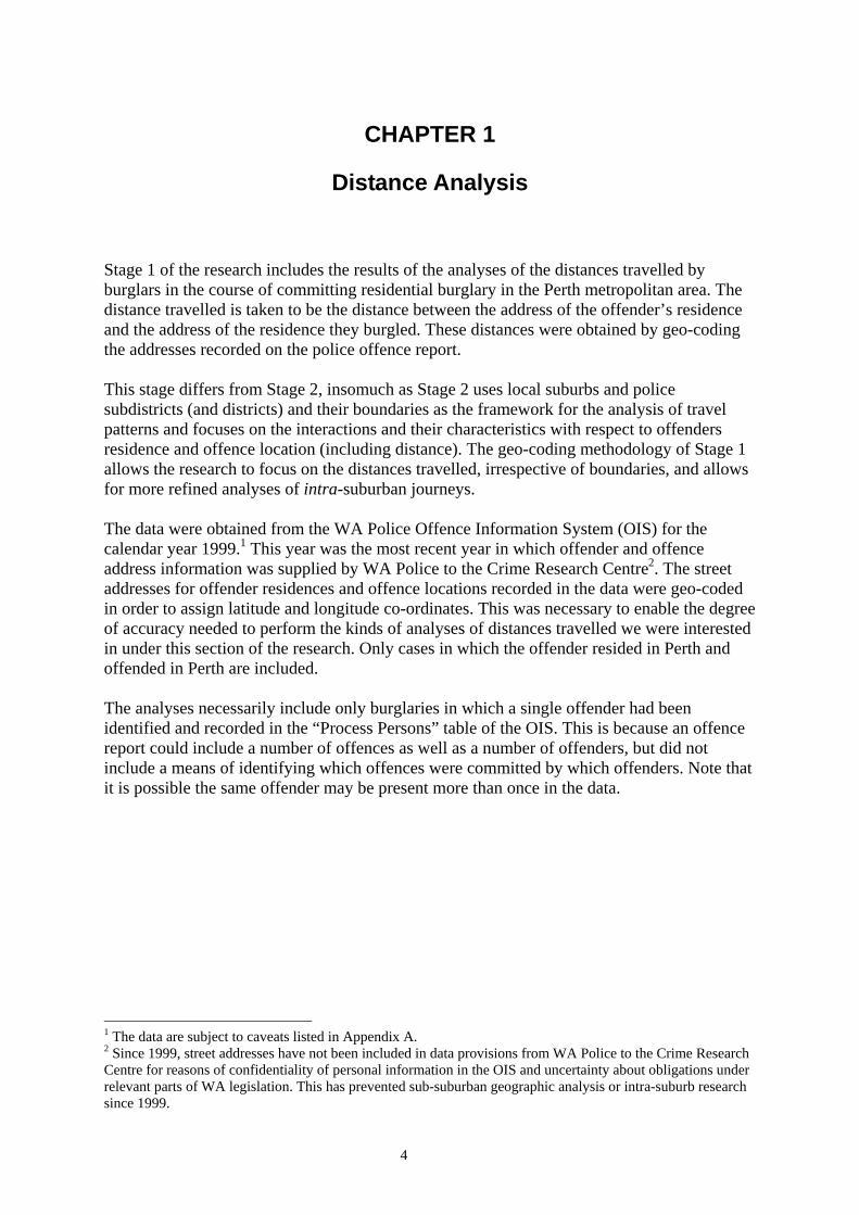
Figure 1.4 highlights as interesting feature of the ages of offenders in ‘short’ distance burglaries, that is, where the distance travelled was less than one kilometre. Offenders aged less than 18 years comprised 35.2 percent of burglaries of any distance, whereas they comprised 47.5 percent of burglaries where the distance travelled was less than one kilometre. There were also differences noted in the other age groups: offenders aged 18 to 29 years comprised 41.7 percent of short distance burglaries, compared with 49.8 percent of all burglaries, and offenders aged 30 years or more comprised 10.8 percent of short distance burglaries, compared with 15.0 percent of all burglaries. This could indicate that younger offenders account for a larger proportion of neighbourhood and intra-suburb burglary. Figure 1.4: Percent of burglaries in offender age-groups, for journeys less than 1km

0%

10%

20%

30%

40%

50%

60%

<18yrs 18-29yrs 30+yrs

Age Group

Perc

ent o

f Bur

glar

ies

<1kmAll Burglaries

The Indigenous status of the offender also contributes to differences in distances travelled in burglaries where the distance was less than one kilometre. In these burglaries, the average distance travelled by non-Indigenous offenders to short distance burglaries was 821 metres, but the average distance travelled by Indigenous offenders was just 151 metres. This indicates that where Indigenous offenders are responsible for locally-sourced burglary, they are more likely to reside in the immediate neighbourhood - perhaps a few houses away.

Distance Decay of Journeys to Residential Burglary The distribution of the distances travelled by offenders to commit residential burglary in Perth follows the familiar distance decay pattern found in many other studies on journeys to burglary. This refers to the fact that the number of burglaries decreases as the distance travelled by offenders increases. This kind of pattern supports the idea in rational choice theory that a potential offender incorporates a consideration of the effort required to commit an offence when deciding whether or not to commit the offence or when deciding between alternative offence choices, viz, that potential offenders are inclined to choose targets that are closer rather than targets that are further away. In this case, the extra effort required to travel to a suburb several kilometres away is a dampening factor on the likelihood of committing an offence there. Figure 1.5 shows the distribution of the distances travelled by offenders to commit residential burglary in Perth. It shows the percentages of all burglaries committed at five-kilometre intervals from the burglar’s residence. It shows that burglaries committed within the first five kilometres of the offender’s residence accounted for two thirds (66.2%) of all burglaries.

9

Figure 1.5: Distribution of distances travelled, for all residential burglary (5km intervals)

0%

20%

40%

60%

80%

100%

5 10 15 20 25 30 35 40 45 50 55 60 65 70

Distance (Km)

Perc

ent o

f Bur

glar

ies

PercentCumulative Percent

Figure 1.6 shows the percentages of all burglaries committed at one-kilometre intervals. It shows that burglaries committed within the first kilometre of the offender’s residence accounted for one third (34.9%) of all burglaries, and about half (47.8%) of all burglaries were committed within two kilometres of the offender’s residence. Figure 1.6: Distribution of distances travelled, for all residential burglary (1km intervals)

0%

20%

40%

60%

80%

100%

0-1 5-6 10-11 15-16 20-21 25-26 30-31 35-36

Distance (Km)

Perc

ent o

f Bur

glar

ies


An interesting phenomenon was found in the distribution of shorter distances to burglary. It was expected that there might be a smaller proportion of burglaries committed very close to the offender’s residence. This stemmed from the notion that burglars might think there are increased chances of being detected and recognised by people in the neighbourhood when committing offences close to home. However, when the distribution of distances travelled was examined at 100-metre intervals, it was found that there was no such ‘home buffer’ effect. As Figure 1.7 shows, the proportions of burglaries that occur within the smallest distance intervals from the offender’s home remain the highest of all proportions in the distribution; specifically, 6.6 percent of these burglaries occurred within 100m of the burglar’s home, and a further 7.3 percent occurred within the next 100 metres. The distance

10

decay pattern is somewhat hidden in Figure 1.6 because the smaller intervals each capture smaller numbers of burglaries, which leads to more natural variability in the percentages; however, as Figures 1.5 and 1.6 show, the distance decay pattern is an inherent trait of the distances offenders travel to commit burglary. There may be some relevance here for crime prevention policy that focuses on neighbourhood strategies. If a significant proportion of burglaries are committed by local residents then this could provide support and justification for the Neighbourhood Watch strategy, because neighbours might have a better chance of recognising potential offenders within their own neighbourhood. The strategy of ‘cocooning’ is also informed by this, viz, if a significant proportion on burglaries are committed by residents in the neighbourhood, it is reasonable to suggest that residences in the immediate surroundings are also likely to be targeted. Figure 1.7: Distribution of distances travelled, for all residential burglary (100m intervals)

0%

10%

20%

30%

40%

50%

0.1 0.4 0.7 1 1.3 1.6 1.9

Distance (Km)

Perc

ent o

f Bur

glar

ies


Even though most burglaries tend to occur relatively close to the offender’s residence, not all are. There may be many reasons why a potential offender would choose to travel greater distances to commit a burglary. For example, the potential for a greater return for the effort expended may entice offenders from relatively distant suburbs to offend in suburbs that are known to have houses that contain more attractive goods or that have goods that are more accessible; for example, a suburb with higher socio-economic status indicator, such as weekly income or number of luxury cars, may have houses that are more likely to contain expensive jewellery (which is a highly prized spoil of burglars because of its monetary value, ease of liquidation and high portability), and so a potential offender may be more attracted to commit a burglary in such a suburb. Furthermore, there may be suburbs that, even though they are not close to an offender’s residence, may be close to the place of their employment or recreation, or perhaps to family or friends’ homes, or that an offender may travel through en route to these destinations. These are the places with which an offender has some familiarity, owing to their daily or weekly routine activities, and, hence, are recalled from their cognitive awareness space when deciding on potential targets for a burglary.

11

In order to highlight how some factors may affect the distance travelled, we will consider the median weekly household income of the target suburb. Figure 1.8 shows the average distances travelled to commit residential burglary by the income group of the target suburb. It reveals a pattern of increasing distances travelled as the income of the target suburb increases. This supports the hypothesis that target affluence has an influence of target choice. Figure 1.8: Target suburb income and distances travelled

0

2

4

6

8

10

12

$300

-$399

$400

-$499

$500

-$599

$600

-$699

$700

-$799

$800

-$999

$1,00

0-$1,1

99

$1,20

0-$1,4

99

$1,50

0-$1,9

99

Median Weekly Household Income of Target Suburb

Ave

rage

Dis

tanc

e (K

m)

Figure 1.9 shows also how the median weekly household income of the target suburb is associated with the distances travelled by the offender. The graph, however, divides all residential burglaries into those that occurred at a distance of less than 10 kilometres and those that occurred at a distance of more than 10 kilometres, and places all suburbs into just three income groups. About two thirds of burglaries in both distance groups occurred in suburbs where the median income was $600-$999. The interesting observation in the graph, however, is how the proportions for the lower and higher income groups change within the two distance groups: for burglaries within 10 kilometres of the offenders residence, lower income suburbs were targeted 18.2 percent of the time, but for burglaries at greater distances, they were targeted only 10.4% of the time. Similarly, for burglaries within 10 kilometres of the offenders residence, higher income suburbs were targeted 12.3 percent of the time, but for burglaries at greater distances, they were targeted 20.2% of the time. A simple statistical procedure, the chi-square test, can indicate the likelihood of obtaining these figures. This test reveals that the probability of obtaining these figures is less than one percent, and so it is very likely that there is some association between the distance travelled and the income of the target suburb.

12

Figure 1.9: Target suburb income and distances travelled

0%

20%

40%

60%

80%

100%

0-10km >10km

Median Weekly Household Income

Perc

ent o

f Bur

glar

ies

$300-$599 $600-$999 $1000-$1999

Figure 1.10 shows the distribution of distances travelled, by the sex of the offender. Male offenders account for a larger proportion of burglaries at distances of less than five kilometres, but female offenders account for larger proportions of burglaries at greater distances. Figure 1.10: Distribution of distances travelled, by offender sex

0%

20%

40%

60%

80%

100%

5 10 15 20 25 30 35 40 45 50

Distance (Km)

Perc

ent o

f Bur

glar

ies

Female Male

13

Figure 1.11 shows the distribution of distances travelled, by the Indigenous status of the offender. It appears that there is not much difference in the distance decay pattern between Indigenous and non-Indigenous offenders. Figure 1.12 zooms in on this same graph to reveal the distribution of distances at smaller distance intervals. It shows that for burglaries within the first 200 metres of the offender’s home, Indigenous offenders account for larger proportions of the burglaries than non-Indigenous offenders. Figure 1.11: Distribution of distances travelled, by offender Indigenous status (5km)

0%

20%

40%

60%

80%

100%

5 10 15 20 25 30 35 40 45 50

Distance (Km)

Perc

ent o

f Bur

glar

ies

Indig. Non-Indig.

Figure 1.12: Distribution of distances travelled, by offender Indigenous status (100m)

0%1%

2%3%

4%5%

6%7%

8%9%

0-0.1 0.5-0.6 1-1.1 1.5-1.6

Distance (Km)

Perc

ent o

f Bur

glar

ies

Indig Non-Indig

14

Figure 1.13 shows the distribution of distances travelled, by the age group of the offender. It shows that offenders aged under 18 years account for a greater proportion of the burglaries at distances of five kilometres or less, and account for smaller proportions at greater distances. Figure 1.14 zooms in on this same graph to reveal the distribution of distances at smaller distance intervals. It shows that, although juvenile offenders account for larger proportions of burglaries between 200 to 700 metres away from the their home, they account for a smaller proportion of burglaries within the first 100 metres of their home. This could indicate a home-buffer effect for juvenile offenders. Figure 1.13: Distribution of distances travelled, by offender age group (5km)

0%

20%

40%

60%

80%

5 10 15 20 25 30 35 40

Distance (Km)

Perc

ent o

f Bur

glar

ies

<18yrs 18-29yrs 30+yrs

Figure 1.14: Distribution of distances travelled, by offender age group (100m)

0%

2%

4%

6%

8%

10%

0-0.1 0.5-0.6 1-1.1

Distance (Km)

Perc

ent o

f Bur

glar

ies Juv 18-29yrs 30+yrs

15

Figure 1.15 shows the distribution of distances travelled, by the time of day that the offence occurred, divided into two groups: day (from 6am to 6pm) and night (from 6pm to 6am).3 It shows that night-time burglaries account for slightly greater proportions of burglaries within the first three kilometres of the offender’s home; overall, however, there is not a significant difference between the distance decay patterns of burglaries occurring during the day and those occurring during the night. Figure 1.15: Distribution of distances travelled, by day and night

0%

5%

10%

15%

20%

25%

30%

35%

40%

0-1 5-6 10-11 15-16

Distance (Km)

Perc

ent o

f Bur

glar

ies

Day Night

Distances Travelled To and From Suburbs Tables 1.1 and 1.2 give a suburb by suburb description of the average distances of journeys to burglary. Table 1.1 shows the average distance travelled to each suburb by offenders, as well as the proportion of its burglaries occurring within two kilometres of the offenders residence. The suburbs in this table are those of the victims, and the distances indicate how far burglars travelled to in order to victimize each of these suburbs. Table 1.2 shows the average distance travelled by burglars, according to where they themselves live, as well as the proportion of burglaries committed within two kilometres of their residence. The suburbs in this table are those of the offenders, and the distances indicate how far burglars from each of these suburbs travelled to victimize other suburbs. The reader should be mindful that there are suburbs that lie on or near the outskirts of the Perth metropolitan area and this fact may partially account for these suburbs ranking highly in one or both of the tables.

3 The specific time of day is not known some burglaries, but the police record the ‘from-time’ and ‘to-time’ of burglaries, where relevant, and this has enabled offences to be grouped into day and night. See Ratcliffe and McCullagh (1998) for techniques for examining this issue.

16

Table 1.1: Average distances (kilometres) travelled by burglars, by victim suburb Suburb Avg

Dist. % less 2km

Alexander Heights

3.3 50.0

Alfred Cove 1.5 50.0 Applecross 3.1 0.0 Armadale 6.1 40.0 Ascot 0.1 100 Ashfield 11.9 0.0 Attadale 3.8 33.3 Balcatta 4.5 71.4 Baldivis 8.7 0.0 Balga 2.4 76.9 Ballajura 2.4 64.7 Bassendean 9.0 40.0 Bayswater 6.0 30.8 Beaconsfield 7.3 33.3 Beckenham 6.6 28.6 Bedford 5.0 50.0 Beechboro 2.3 73.9 Beeliar 1.0 100 Beldon 2.7 33.3 Bellevue 0.9 100 Belmont 6.7 42.9 Bentley 5.2 55.6 Bibra Lake 4.2 50.0 Bicton 1.0 100 Booragoon 9.4 0.0 Brentwood 5.7 0.0 Bull Creek 7.0 33.3 Bullsbrook 51.6 0.0 Burswood 7.6 0.0 Byford 6.4 0.0 Calista 0.1 100 Canning Vale 12.9 33.3 Cannington 1.4 50.0 Carine 2.6 66.7 Carlisle 4.8 0.0 Carramar 1.6 100 Casuarina 22.1 0.0 City Beach 5.7 25.0 Claremont 11.4 0.0 Clarkson 4.0 84.6 Cloverdale 4.8 66.7 Como 9.3 25.0 Connolly 0.2 100 Coolbellup 0.4 100 Coolbinia 9.0 0.0 Cooloongup 4.6 11.1 Cottesloe 12.9 0.0 Craigie 12.3 0.0 Currambine 25.3 0.0 Daglish 9.0 0.0 Dalkeith 9.6 33.3 Darling Downs

23.9 0.0

Darlington 10.7 0.0 Dianella 4.5 18.2

Suburb Avg Dist.

% less 2km

Doubleview 0.8 80.0 Duncraig 3.1 0.0 East Cannington

1.2 100

East Fremantle

8.0 0.0

East Perth 7.9 0.0 East Victoria Park

5.4 21.4

Edgewater 1.1 100 Ellenbrook 0.0 100 Ferndale 23.8 33.3 Floreat 12.9 0.0 Forrestdale 9.3 0.0 Forrestfield 5.1 60.0 Fremantle 4.5 60.0 Girrawheen 2.1 86.7 Glendalough 23.9 0.0 Gooseberry Hill

6.7 40.0

Gosnells 3.9 41.2 Greenwood 2.0 50.0 Guilderton 59.1 0.0 Guildford 4.2 42.9 Gwelup 7.0 0.0 Hamilton Hill 1.9 80.0 Heathridge 6.0 50.0 Helena Valley

0.0 100

Henley Brook 8.0 0.0 High Wycombe

6.0 55.6

Highgate 8.7 33.3 Hillarys 9.8 16.7 Hillman 3.8 0.0 Hilton 1.5 83.3 Hope Valley 0.3 100 Huntingdale 2.9 70.0 Inglewood 6.8 0.0 Innaloo 7.1 50.0 Jandakot 5.4 0.0 Jolimont 4.2 0.0 Joondalup 5.0 72.7 Joondanna 5.1 0.0 Kalamunda 3.7 80.0 Kallaroo 5.7 0.0 Karawara 8.6 0.0 Kardinya 9.6 12.5 Karrinyup 9.7 20.0 Kelmscott 4.3 50.0 Kensington 0.2 100 Kenwick 4.7 33.3 Kewdale 6.0 40.0 Kiara 3.6 50.0 Kingsley 5.1 44.4 Kinross 15.4 0.0 Koondoola 3.6 82.4

Suburb Avg Dist.

% less 2km

Koongamia 6.4 66.7 Lancelin 0.2 100 Langford 5.3 66.7 Lathlain 4.1 0.0 Leda 2.8 0.0 Leederville 11.2 20.0 Leeming 6.8 35.7 Lesmurdie 0.9 81.8 Lockridge 5.3 62.5 Lynwood 0.7 100 Maddington 0.5 98.7 Manning 9.5 0.0 Marangaroo 3.1 0.0 Marmion 2.4 33.3 Martin 4.8 0.0 Maylands 5.6 47.1 Medina 8.0 0.0 Melville 1.3 66.7 Menora 13.2 50.0 Merriwa 12.2 75.0 Middle Swan 5.5 40.0 Midland 2.7 76.9 Midvale 3.8 40.0 Mindarie 6.0 0.0 Mirrabooka 0.9 92.3 Morley 6.1 53.8 Mosman Park 9.2 50.0 Mount Claremont

7.3 50.0

Mount Hawthorn

5.5 33.3

Mount Helena

28.7 0.0

Mount Lawley

5.7 47.4

Mount Pleasant

6.5 0.0

Mullaloo 1.1 100 Mundaring 7.6 0.0 Munster 19.5 0.0 Naval Base 0.0 100 Nedlands 18.6 0.0 Neerabup 15.0 33.3 Nollamara 1.5 71.4 Noranda 5.8 16.7 North Beach 8.5 0.0 North Fremantle

16.0 0.0

North Perth 5.1 44.4 Northbridge 8.2 33.3 Oakford 16.5 0.0 Ocean Reef 9.4 50.0 Orange Grove 0.6 100 Orelia 5.5 83.3 Osborne Park 6.2 37.5 Padbury 9.1 45.5 Palmyra 7.1 66.7

Suburb Avg Dist.

% less 2km

Parkwood 16.5 40.0 Parmelia 0.1 100 Perth 10.8 18.8 Queens Park 1.7 83.3 Quinns Rock 10.0 50.0 Redcliffe 1.9 77.8 Riverton 3.9 40.0 Rivervale 7.2 29.4 Rockingham 9.4 45.0 Roleystone 17.2 0.0 Rossmoyne 15.7 0.0 Rottnest Island

24.7 0.0

Safety Bay 1.9 33.3 Saint James 0.1 100 Salter Point 7.8 0.0 Samson 17.8 0.0 Sawyers Valley

0.8 100

Scarborough 5.9 54.5 Serpentine 20.7 0.0 Shelley 1.7 100 Shenton Park 18.8 0.0 Shoalwater 11.9 25.0 Sorrento 3.4 36.4 South Fremantle

8.2 50.0

South Lake 2.8 35.7 South Perth 12.8 0.0 Spearwood 9.2 0.0 Stirling 1.4 50.0 Stratton 8.9 71.4 Subiaco 14.3 0.0 Success 2.0 50.0 Swan View 9.4 50.0 Swanbourne 19.6 0.0 Thornlie 4.3 36.4 Trigg 4.9 33.3 Tuart Hill 3.7 83.3 Two Rocks 0.0 100 Victoria Park 15.3 0.0 Waikiki 7.9 30.0 Wanneroo 6.6 66.7 Warnbro 18.8 16.7 Warwick 16.9 0.0 Waterman 9.2 0.0 Wattleup 8.3 0.0 Wellard 15.8 0.0 Welshpool 3.3 0.0 Wembley 9.1 20.0 Wembley Downs

2.0 33.3

West Midland 0.6 100

17

Table 1.2: Average distances (kilometres) travelled by burglars, by offender suburb

Suburb Avg Dist.

% less 2km

Alexander Heights

0.4 100

Armadale 10.3 25.8 Ascot 1.9 50.0 Ashfield 7.8 0.0 Attadale 4.0 22.7 Atwell 11.2 0.0 Balcatta 7.9 50.0 Balga 8.4 26.1 Ballajura 3.5 73.3 Bassendean 8.0 42.9 Bayswater 6.4 20.0 Beaconsfield 4.9 50.0 Beckenham 13.3 60.0 Bedford 0.2 100 Beechboro 3.1 73.9 Beeliar 2.8 68.6 Beldon 15.8 0.0 Bellevue 9.3 25.0 Belmont 5.8 30.0 Bentley 3.6 45.5 Bibra Lake 1.7 65.0 Bicton 4.0 0.0 Bull Creek 4.9 66.7 Burswood 1.6 100 Calista 10.0 50.0 Canning Vale 13.7 22.2 Cannington 8.8 33.3 Carine 3.0 0.0 Carlisle 5.2 0.0 Casuarina 35.7 0.0 Caversham 5.3 0.0 Claremont 1.3 100 Clarkson 5.1 85.7 Cloverdale 9.0 15.4 Como 6.1 25.0 Connolly 0.2 100 Coolbellup 4.4 50.0 Cooloongup 13.3 16.7 Cottesloe 9.1 0.0 Craigie 8.5 33.3 Currambine 11.7 0.0 Darlington 26.6 0.0 Dianella 4.0 16.7 Doubleview 4.8 60.0 Duncraig 5.9 25.0 East Cannington

11.5 0.0

East Fremantle

14.5 0.0

East Perth 8.0 0.0 East Victoria Park

3.9 50.0

Eden Hill 0.7 100 Edgewater 3.6 50.0 Ellenbrook 10.5 50.0

Suburb Avg Dist.

% less 2km

Embleton 7.7 0.0 Floreat 1.9 100 Forrestfield 3.3 60.0 Fremantle 12.6 36.4 Girrawheen 6.5 37.5 Glendalough 14.4 0.0 Gooseberry Hill

6.9 50.0

Gosnells 7.2 46.7 Greenwood 6.8 25.0 Guildford 6.8 60.0 Gwelup 3.7 0.0 Hamersley 2.8 0.0 Hamilton Hill 7.2 50.0 Heathridge 4.5 58.3 Helena Valley

10.7 33.3

Herne Hill 3.0 0.0 High Wycombe

0.8 83.3

Highgate 2.5 50.0 Hillarys 0.4 100 Hillman 2.6 0.0 Hilton 4.5 27.3 Hope Valley 0.3 100 Huntingdale 0.3 100 Iluka 23.8 0.0 Inglewood 11.9 0.0 Innaloo 2.3 28.6 Jandakot 10.1 0.0 Joondalup 4.1 88.9 Joondanna 19.3 0.0 Kalamunda 1.1 77.8 Kallaroo 3.5 0.0 Karawara 2.8 0.0 Kardinya 21.6 0.0 Karrinyup 11.4 33.3 Kelmscott 5.4 62.5 Kensington 12.6 12.5 Kenwick 7.2 50.0 Kewdale 4.0 33.3 Kingsley 3.3 50.0 Kinross 2.1 0.0 Koondoola 2.6 74.1 Koongamia 13.4 50.0 Lancelin 0.2 100 Langford 2.1 60.0 Lathlain 13.1 0.0 Leda 21.1 0.0 Leederville 0.0 100 Leeming 2.6 50.0 Lesmurdie 2.3 85.7 Lockridge 3.7 43.8 Lynwood 6.9 40.0 Maddington 2.3 80.9 Maida Vale 9.7 50.0

Suburb Avg Dist.

% less 2km

Manning 9.2 12.5 Marangaroo 11.4 0.0 Marmion 0.8 100 Martin 26.2 0.0 Maylands 9.1 35.9 Medina 10.4 50.0 Melville 0.4 100 Menora 3.3 25.0 Merriwa 7.3 40.0 Middle Swan 7.6 25.0 Midland 5.7 70.6 Midvale 6.1 66.7 Mirrabooka 3.5 52.6 Morley 8.5 33.3 Mosman Park 0.3 100 Mount Claremont

0.8 100

Mount Hawthorn

0.3 100

Mount Helena

7.6 0.0

Mount Lawley

2.8 75.0

Mullaloo 26.2 0.0 Myaree 0.9 100 Naval Base 0.0 100 Nedlands 7.9 0.0 Neerabup 0.9 100 Nollamara 4.3 50.0 Noranda 0.6 100 North Beach 3.6 13.3 North Lake 17.5 0.0 Northbridge 2.6 50.0 Ocean Reef 1.5 100 Orelia 8.5 37.5 Osborne Park 7.7 62.5 Padbury 1.8 57.1 Parkwood 18.8 33.3 Parmelia 9.5 44.4 Perth 3.7 33.3 Port Kennedy 7.2 0.0 Queens Park 0.5 100 Quinns Rock 1.5 71.4 Redcliffe 4.3 70.0 Riverton 0.8 100 Rivervale 14.3 26.7 Rockingham 7.0 84.6 Roleystone 22.1 0.0 Safety Bay 4.1 0.0 Saint James 5.8 22.2 Sawyers Valley

0.8 100

Scarborough 3.7 60.9 Serpentine 36.7 0.0 Shoalwater 2.9 33.3 South Fremantle

9.4 0.0

Suburb Avg Dist.

% less 2km

South Lake 4.4 30.0 South Perth 8.8 0.0 Spearwood 11.9 0.0 Stirling 5.2 50.0 Stratton 2.9 83.3 Swan View 21.1 22.2 Thornlie 7.2 35.7 Trigg 0.0 100 Tuart Hill 7.8 55.6 Two Rocks 42.5 25.0 Waikiki 1.7 33.3 Wandi 20.7 0.0 Wanneroo 6.7 40.0 Warnbro 4.2 20.0 Warwick 19.9 50.0 Wembley 10.2 0.0 Wembley Downs

0.1 100

West Leederville

6.0 0.0

West Perth 13.8 0.0 Westfield 3.0 50.0 Westminster 4.1 66.7 White Gum Valley

18.5 0.0

Willagee 2.6 77.8 Willetton 3.8 71.4 Wilson 1.6 100 Winthrop 0.0 100 Woodlands 21.0 0.0 Woodvale 0.7 100 Yangebup 8.5 42.9 Yokine 4.6 50.0

18

CHAPTER 2

Area by Area Analysis This chapter includes the results of the research that used police subdistricts and districts as the framework for the analysis of travel patterns. The main objective was to gain insights into where offenders come from and where offenders go to offend. It focussed on the matrix of interactions between police subdistricts with respect to offenders residence and offence location. Offences in an area that are committed by offenders who live in that area are call endogenous offences and offences in an area that are committed by offenders who do not live in that area are call exogenous offences. When forming burglary prevention strategies aimed at particular areas, it is important to understand issues related to the source of the burglaries, such as where the offenders who offend in those areas come from, and to where offenders in those areas go to offend. For example, if the strategy is aimed at young offenders in a particular suburb, it may not be very effective at reducing burglary in that suburb if most of the burglaries are committed by offenders who live in other suburbs. In this case other kinds of strategies may be more effective. To this end, this chapter focuses on the interactions between the victim subdistrict and the offender subdistrict. Originally, the analyses used suburbs as the basis for analysis, but it was requested by the Office of Crime Prevention that police subdistrict and district boundaries be used instead. Notwithstanding this, there is one section in which selected suburbs each have listed the ‘source’ suburbs from which offenders travelled to offend in them. The change of focus onto police subdistricts may be beneficial, not just from a presentational perspective but, more importantly, because many of the operational initiatives that could benefit from this intelligence would involve local police and other agencies at the subdistrict level. Further, initiatives from within these geographic levels may not be readily informed as to the source of their burglaries, endogenous or exogenous; and so having this ‘bird’s eye’ view of burglary travel patterns over all metropolitan subdistricts is very useful. The change to police subdistrict boundaries was also fortuitous, as the suburb-by-suburb analysis proved to be too cumbersome to analyse and present, owing to the large number of suburbs involved. The information will be presented mainly in the form of tables that show the interactions of subdistricts and districts and the contributions each makes to the total burglary of others. These tables will be invaluable resources for crime prevention strategies and can be updated to evaluate the effectiveness of prevention programs in any of the areas. The data come from crimes reported to WA Police in 2001 and includes all residential burglary in Perth for which there was exactly one processed person on the police report.

19

District-level Analysis This section helps to inform us about where offenders come from to commit a burglary in an area and where offenders in an area go to, with respect to police districts. Table 2.1a shows, for each police district that offences were committed in, the proportion made by each of the police districts where the offenders came from in order to offend within that district. For example, for burglaries committed in the Central Metropolitan district, the East Metropolitan district contributed 7.8 percent of those burglaries, while the West Metropolitan district contributed 25.1 percent. Of all the districts, the Central Metropolitan district had the lowest rate of endogenous offences, that is, the proportion of its offences committed by local (resident) offenders (30.5%), while the South Metropolitan district had the highest (87.4%). Table 2.1a: Police district of offender residence, by police district of target

District of Offender Residence CEN

TRA

L M

ETR

OPO

LITA

N

EAST

M

ETR

OPO

LITA

N

NO

RTH

WES

T M

ETR

OPO

LITA

N

SOU

TH E

AST

M

ETR

OPO

LITA

N

SOU

TH

MET

RO

POLI

TAN

WES

T M

ETR

OPO

LITA

N

Perth

met

ro.

CENTRAL METROPOLITAN 30.5% 0.5% 1.2% 1.7% 1.1% 3.2% 4.5% EAST METROPOLITAN 7.8% 71.6% 5.3% 3.5% 0.6% 6.1% 12.8% NORTH WEST METROPOLITAN 8.4% 2.3% 72.8% 3.1% 0.3% 11.1% 14.3% SOUTH EAST METROPOLITAN 16.8% 6.4% 3.3% 79.7% 4.9% 10.7% 25.9% SOUTH METROPOLITAN 11.4% 3.2% 0.4% 5.2% 87.4% 0.7% 21.2% WEST METROPOLITAN 25.1% 16.1% 16.9% 6.8% 5.7% 68.2% 21.3% Total 100.0% 100.0% 100.0% 100.0% 100.0% 100.0% 100.0%

Table 2.1b helps to inform us about where locally resident offenders go to. It shows, for each police district that offenders live in, the proportion of their offences committed in each of the police districts. For example, for the burglary offenders living in the Central Metropolitan district, they committed 1.3 percent of all their offences in the East Metropolitan district, while they committed 12.0 percent in the West Metropolitan district. Of all the districts, the West Metropolitan district had the lowest proportion of endogenous offending, that is, offenders committing burglaries within its own district (53.4%), while the South Metropolitan district had the highest (85.7%). Table 2.1b: Police district of burglary locations, by police district of offender residence

District of Offence Location CEN

TRA

L M

ETR

OPO

LITA

N

EAST

M

ETR

OPO

LITA

N

NO

RTH

WES

T M

ETR

OPO

LITA

N

SOU

TH E

AST

M

ETR

OPO

LITA

N

SOU

TH

MET

RO

POLI

TAN

WES

T M

ETR

OPO

LITA

N

Perth

met

ro.

CENTRAL METROPOLITAN 68.0% 6.0% 5.8% 6.4% 5.3% 11.7% 9.9%

EAST METROPOLITAN 1.3% 72.2% 2.1% 3.2% 2.0% 9.8% 13.0%

NORTH WEST METROPOLITAN 4.0% 6.0% 73.4% 1.8% 0.3% 11.5% 14.5%

SOUTH EAST METROPOLITAN 9.3% 6.9% 5.4% 77.7% 6.2% 8.1% 25.2%

SOUTH METROPOLITAN 5.3% 0.9% 0.4% 3.9% 85.7% 5.6% 20.8%

WEST METROPOLITAN 12.0% 7.9% 12.9% 6.9% 0.6% 53.4% 16.7%

Total 100.0% 100.0% 100.0% 100.0% 100.0% 100.0% 100.0%

20

Subdistrict-level Analysis This section helps to inform us about where offenders come from to commit burglary in an area and where offenders in an area go to, with respect to police subdistricts. The subdistricts will be grouped according to the district they fall into, for example, the Subiaco subdistrict falls into the Central Metropolitan district. Each district will be treated separately and for each district two tables will be presented: one for where offenders come from and one for where local offenders go to. Central Metropolitan district Table 2.2a shows, for burglaries committed in the Central Metropolitan police district, the subdistricts of where offenders came from and the proportions of all offences in the Central Metropolitan district they contributed. The subdistrict of Subiaco contributed 9.6 percent of burglaries committed in the Central Metropolitan district. Table 2.2a: Subdistrict of offenders for burglaries committed in the Central Metropolitan district

Subdistrict Contribution to all burglaries in the Central Metropolitan district

SUBIACO 9.6% COTTESLOE 9.0% BAYSWATER 6.6% PERTH 5.4% KENSINGTON 5.4% COCKBURN 5.4% SCARBOROUGH 4.8% BELMONT 4.8% LEEDERVILLE 4.8% INGLEWOOD 4.8% MORLEY 4.2% WARWICK 3.6% MIRRABOOKA 3.6% MIDLAND 3.6% GOSNELLS 3.0% HILLARYS 2.4% BALLAJURA 2.4% WEMBLEY 1.8% CANNINGTON 1.8% FREMANTLE 1.8% ARMADALE 1.8% CLARKSON 1.8% PALMYRA 1.8% HILTON 1.2% KIARA 1.2% STIRLING 1.2% FORRESTFIELD 0.6% MURDOCH 0.6% JOONDALUP 0.6% ROCKINGHAM 0.6%

21

Table 2.2b shows, for all offenders residing in the Central Metropolitan police district, the subdistricts in which they offended and the proportion of the total of their offences each subdistrict contributed. Offenders residing in the Central Metropolitan police district committed 26.9 percent of their burglaries in the Perth subdistrict. Table 2.2b: Subdistrict of burglary locations committed by Central Metropolitan offenders

Subdistrict

Proportion of all burglaries committed by Central Metropolitan district offenders

PERTH 26.9% COTTESLOE 19.2% LEEDERVILLE 11.5% WEMBLEY 5.1% KENSINGTON 5.1% WANNEROO 3.8% BAYSWATER 3.8% FREMANTLE 2.6% MIRRABOOKA 2.6% SUBIACO 2.6% STIRLING 2.6% SCARBOROUGH 2.6% GOSNELLS 1.3% CANNINGTON 1.3% PALMYRA 1.3% MURDOCH 1.3% MUNDARING 1.3% BELMONT 1.3%

22

East Metropolitan district Table 2.3a shows, for burglaries committed in the East Metropolitan police district, the subdistricts of where offenders came from and the proportions of all offences in the East Metropolitan district they contributed. The subdistrict of Midland contributed 27.5 percent of burglaries committed in the East Metropolitan district. Table 2.3a: Subdistrict of offenders for burglaries committed in the East Metropolitan district

Subdistrict Contribution to all burglaries in the East Metropolitan district

MIDLAND 27.5% KIARA 19.7% KALAMUNDA 10.6% MORLEY 9.6% FORRESTFIELD 7.8% BALLAJURA 6.0% BELMONT 2.8% MIRRABOOKA 2.8% BAYSWATER 2.3% WARWICK 1.8% CANNINGTON 1.8% FREMANTLE 1.8% STIRLING 0.9% GOSNELLS 0.9% INGLEWOOD 0.5% ARMADALE 0.5% KENSINGTON 0.5% KWINANA 0.5% PERTH 0.5% ROCKINGHAM 0.5% COCKBURN 0.5% WANNEROO 0.5%

23

Table 2.3b shows, for all offenders residing in the East Metropolitan police district, the subdistricts in which they offended and the proportion of the total of their offences each subdistrict contributed. Offenders residing in the East Metropolitan police district committed 26.9 percent of their burglaries in the Perth subdistrict. Table 2.3b: Subdistrict of burglary locations committed by East Metropolitan offenders

Subdistrict

Proportion of all burglaries committed by East Metropolitan district offenders

MIDLAND 26.8% KIARA 17.3% KALAMUNDA 10.5% FORRESTFIELD 8.2% BALLAJURA 6.4% JOONDALUP 4.1% MORLEY 3.2% BAYSWATER 3.2% PERTH 2.7% KENSINGTON 2.7% MUNDARING 1.8% BELMONT 1.8% WARWICK 1.4% CANNINGTON 1.4% WEMBLEY 0.9% LEEDERVILLE 0.9% COTTESLOE 0.9% GOSNELLS 0.5% INGLEWOOD 0.5% ROCKINGHAM 0.5% SCARBOROUGH 0.5% STIRLING 0.5% SUBIACO 0.5% WANNEROO 0.5% MURDOCH 0.5% ARMADALE 0.5%

24

North West Metropolitan district Table 2.4a shows, for burglaries committed in the North West Metropolitan police district, the subdistricts of where offenders came from and the proportions of all offences in the North West Metropolitan district they contributed. The subdistrict of Warwick contributed 30.5 percent of burglaries committed in the North West Metropolitan district. Table 2.4a: Subdistrict of offenders for burglaries committed in the North West Metro. district

Subdistrict

Contribution to all burglaries in the North West Metropolitan district

WARWICK 30.5% CLARKSON 15.6% JOONDALUP 14.4% SCARBOROUGH 5.8% HILLARYS 5.8% WANNEROO 5.3% MIRRABOOKA 5.3% MIDLAND 4.9% STIRLING 2.5% BAYSWATER 2.5% TWO ROCKS 1.2% GOSNELLS 1.2% LEEDERVILLE 1.2% BELMONT 1.2% BALLAJURA 0.4% MORLEY 0.4% CANNINGTON 0.4% INGLEWOOD 0.4% KENSINGTON 0.4% COCKBURN 0.4%

25

Table 2.4b shows, for all offenders residing in the North West Metropolitan police district, the subdistricts in which they offended and the proportion of the total of their offences each subdistrict contributed. Offenders residing in the North West Metropolitan police district committed 26.9 percent of their burglaries in the Warwick subdistrict. Table 2.4b: Subdistrict of burglary locations committed by North West Metropolitan offenders

Subdistrict

Proportion of all burglaries committed by North West Metropolitan district offenders

WARWICK 27.5% JOONDALUP 15.2% CLARKSON 13.9% HILLARYS 9.8% WANNEROO 5.3% MIRRABOOKA 3.7% MORLEY 3.3% PERTH 2.9% KENSINGTON 2.9% INGLEWOOD 2.9% SUBIACO 1.6% KIARA 1.2% SCARBOROUGH 1.2% CANNINGTON 1.2% BAYSWATER 0.8% COTTESLOE 0.8% TWO ROCKS 0.8% BELMONT 0.8% STIRLING 0.8% MIDLAND 0.4% FORRESTFIELD 0.4% GOSNELLS 0.4% MURDOCH 0.4% WEMBLEY 0.4%

26

South East Metropolitan district Table 2.5a shows, for burglaries committed in the South East Metropolitan police district, the subdistricts of where offenders came from and the proportions of all offences in the South East Metropolitan district they contributed. The subdistrict of Gosnells contributed 37.7 percent of burglaries committed in the South East Metropolitan district. Table 2.5a: Subdistrict of offenders for burglaries committed in the South East Metro. district

Subdistrict

Contribution to all burglaries in the South East Metropolitan district

GOSNELLS 37.7% ARMADALE 14.6% KENSINGTON 10.1% BELMONT 9.4% CANNINGTON 7.8% MIRRABOOKA 3.1% KIARA 1.7% BAYSWATER 1.7% WARWICK 1.4% FORRESTFIELD 1.4% HILTON 1.2% PERTH 1.2% ROCKINGHAM 0.9% PALMYRA 0.9% MORLEY 0.9% WANNEROO 0.7% INGLEWOOD 0.7% KWINANA 0.7% WEMBLEY 0.5% MURDOCH 0.5% COCKBURN 0.5% FREMANTLE 0.5% JOONDALUP 0.5% MIDLAND 0.5% TWO ROCKS 0.5% SCARBOROUGH 0.2% STIRLING 0.2%

27

Table 2.5b shows, for all offenders residing in the South East Metropolitan police district, the subdistricts in which they offended and the proportion of the total of their offences each subdistrict contributed. Offenders residing in the South East Metropolitan police district committed 37.0 percent of their burglaries in the Gosnells subdistrict. Table 2.5b: Subdistrict of burglary locations committed by South East Metropolitan offenders

Subdistrict

Proportion of all burglaries committed by South East Metropolitan district offenders

GOSNELLS 37.0% ARMADALE 14.5% KENSINGTON 9.7% CANNINGTON 8.7% BELMONT 7.8% PERTH 2.3% BAYSWATER 2.1% MURDOCH 1.8% COTTESLOE 1.8% SUBIACO 1.4% STIRLING 1.1% SCARBOROUGH 1.1% MIDLAND 1.1% INGLEWOOD 1.1% WARWICK 0.9% ROCKINGHAM 0.9% FORRESTFIELD 0.9% MORLEY 0.9% WEMBLEY 0.7% KALAMUNDA 0.5% MIRRABOOKA 0.5% COCKBURN 0.5% HILLARYS 0.5% KIARA 0.5% CLARKSON 0.5% LEEDERVILLE 0.2% PALMYRA 0.2% BALLAJURA 0.2% FREMANTLE 0.2% KWINANA 0.2%

28

South Metropolitan district Table 2.6a shows, for burglaries committed in the South Metropolitan police district, the subdistricts of where offenders came from and the proportions of all offences in the South Metropolitan district they contributed. The subdistrict of Cockburn contributed 19.5 percent of burglaries committed in the South Metropolitan district. Table 2.6a: Subdistrict of offenders for burglaries committed in the South Metro. district

Subdistrict Contribution to all burglaries in the South Metropolitan district

COCKBURN 19.5% ROCKINGHAM 17.5% MURDOCH 16.0% KWINANA 10.9% PALMYRA 10.0% HILTON 7.2% FREMANTLE 6.3% BAYSWATER 2.6% BELMONT 1.7% KENSINGTON 1.4% SCARBOROUGH 1.1% STIRLING 0.9% CANNINGTON 0.6% MIDLAND 0.6% MIRRABOOKA 0.6% MORLEY 0.6% GOSNELLS 0.6% ARMADALE 0.6% PERTH 0.6% WARWICK 0.3% COTTESLOE 0.3% LEEDERVILLE 0.3%

29

Table 2.6b shows, for all offenders residing in the South Metropolitan police district, the subdistricts in which they offended and the proportion of the total of their offences each subdistrict contributed. Offenders residing in the South Metropolitan police district committed 19.2 percent of their burglaries in the Rockingham subdistrict. Table 2.6b: Subdistrict of burglary locations committed by South Metropolitan offenders

Subdistrict

Proportion of all burglaries committed by South Metropolitan district offenders

ROCKINGHAM 19.2% MURDOCH 19.0% COCKBURN 14.6% PALMYRA 8.4% FREMANTLE 7.9% KWINANA 7.3% HILTON 6.2% COTTESLOE 3.3% KENSINGTON 2.7% CANNINGTON 1.9% KIARA 1.1% SUBIACO 0.8% ARMADALE 0.8% LEEDERVILLE 0.5% MIDLAND 0.5% PERTH 0.5% BELMONT 0.3% FORRESTFIELD 0.3% BAYSWATER 0.3% SCARBOROUGH 0.3% GOSNELLS 0.3% WARWICK 0.3%

30

West Metropolitan district Table 2.7a shows, for burglaries committed in the West Metropolitan police district, the subdistricts of where offenders came from and the proportions of all offences in the West Metropolitan district they contributed. The subdistrict of Mirrabooka contributed 20.4 percent of burglaries committed in the West Metropolitan district. Table 2.7a: Subdistrict of offenders for burglaries committed in the West Metro. district

Subdistrict Contribution to all burglaries in the West Metropolitan district

MIRRABOOKA 20.4% BAYSWATER 13.9% SCARBOROUGH 11.4% MORLEY 11.4% WARWICK 8.9% STIRLING 8.2% MIDLAND 3.6% KENSINGTON 3.2% INGLEWOOD 2.9% BELMONT 2.1% GOSNELLS 2.1% CANNINGTON 1.8% JOONDALUP 1.8% KIARA 1.8% PERTH 1.4% ARMADALE 1.4% WEMBLEY 0.7% FREMANTLE 0.4% LEEDERVILLE 0.4% KALAMUNDA 0.4% HILLARYS 0.4% HILTON 0.4% FORRESTFIELD 0.4% SUBIACO 0.4% COTTESLOE 0.4%

31

Table 2.7b shows, for all offenders residing in the West Metropolitan police district, the subdistricts in which they offended and the proportion of the total of their offences each subdistrict contributed. Offenders residing in the West Metropolitan police district committed 13.7 percent of their burglaries in the Mirrabooka subdistrict. Table 2.7b: Subdistrict of burglary locations committed by West Metropolitan offenders

Subdistrict

Proportion of all burglaries committed by West Metropolitan district offenders

MIRRABOOKA 13.7% SCARBOROUGH 10.3% MORLEY 8.1% BAYSWATER 7.8% STIRLING 6.7% INGLEWOOD 6.7% KIARA 5.9% LEEDERVILLE 5.3% WARWICK 3.6% JOONDALUP 3.6% PERTH 3.4% HILLARYS 3.4% KENSINGTON 3.1% WEMBLEY 2.2% GOSNELLS 2.0% FREMANTLE 2.0% BELMONT 2.0% HILTON 2.0% MIDLAND 1.7% CANNINGTON 0.8% BALLAJURA 0.8% KALAMUNDA 0.8% COCKBURN 0.8% CLARKSON 0.6% FORRESTFIELD 0.6% COTTESLOE 0.6% PALMYRA 0.3% ARMADALE 0.3% ROCKINGHAM 0.3% SUBIACO 0.3% WANNEROO 0.3% MURDOCH 0.3%

32

Suburb-level Analysis for Selected Suburbs This section helps to inform us about where offenders come from to commit a burglary in each of the following suburbs: Como, Gosnells, Bentley, Rivervale, Manning and Bicton. Owing to the fact that suburbs cover relatively smaller geographical areas than Police sub-districts, the tables listed below contain only the counts of offenders from each source suburb, and often these counts are small. Table 2.8: Suburb of offenders for burglaries committed in the suburb of Como

Source suburb Count BALGA 2 WILLAGEE 1 ATTADALE 1 BEECHBORO 1 CANNINGTON 1 COMO 1 GERALDTON 1 MANNING 1 MAYLANDS 1 QUEENS PARK 1 WEMBLEY 1

Table 2.9: Suburb of offenders for burglaries committed in the suburb of Gosnells

Source suburb Count GOSNELLS 11 MADDINGTON 7 ARMADALE 2 VICTORIA PARK 1 MOUNT LAWLEY 1

Table 2.10: Suburb of offenders for burglaries committed in the suburb of Bentley

Source suburb Count BENTLEY 5 WANDI 1 EAST VICTORIA PARK 1 KARAWARA 1 MAYLANDS 1 SAINT JAMES 1 TUART HILL 1

33

Table 2.11: Suburb of offenders for burglaries committed in the suburb of Rivervale

Source suburb Count RIVERVALE 5 BELLEVUE 2 WANNEROO 1 BALGA 1 BURSWOOD 1 CARLISLE 1 FORRESTFIELD 1 KENSINGTON 1 KEWDALE 1 LOCKRIDGE 1 MANNING 1 MOUNT LAWLEY 1 MULLALOO 1 NORTHBRIDGE 1 PARKWOOD 1 ASCOT 1 SAINT JAMES 1

Table 2.12: Suburb of offenders for burglaries committed in the suburb of Manning

Source suburb Count LYNWOOD 1 BALGA 1 CARLISLE 1

Table 2.13: Suburb of offenders for burglaries committed in the suburb of Bicton

Source suburb Count ATTADALE 3 BIBRA LAKE 1

Table 2.14: Suburb of offenders for burglaries committed in the suburb of Armadale

Source suburb Count ARMADALE 16 WESTFIELD 5 KELMSCOTT 4 BENTLEY 1 FORRESTDALE 1 FREMANTLE 1 GOSNELLS 1 CLOVERDALE 1 MAYLANDS 1

34

CHAPTER 3

Offender Interview Questions This chapter deals with aspects of the burglar’s journey from crime, aspects related the ‘getaway’ after the offence and other relevant information. The information was obtained from the interviews with 241 offenders conducted as part of another, but related, research project on the disposal of stolen goods in Perth for the Office of Crime Prevention. Results from that project can be found in the 2006 report “Known burglars and the stolen goods market in Western Australia” by Anna Ferrante and Joe Clare of the Crime Research Centre. (See that report for information about methodology, interviewee demographic characteristics and other results). The interviews included questions related to the offender’s journey and travel patterns immediately after their most recent burglary. This information is invaluable for uncovering patterns of burglars’ modus operandi and of travel patterns with respect to proximity of place of residence, place of offence and other places relevant to the disposal of stolen goods. The results will be presented one question at a time, with commentary and interpretation inserted, as relevant. Findings for most interview questions will be classified according to the age group of the offender (adults and young offenders) and the Indigenous status of the offender.

35

General What type of place was burgled? This question deals with the type of place burgled. Table 3.1 shows that houses where the target in almost two thirds of cases (63.4%), and offices, factories and places selling alcohol each accounted for less than five percent of cases. Figure 3.1 shows the same information, but broken down by the age group and the Indigenous status of the offender. Older offenders were more likely to burgle places selling alcohol than were younger offenders, while younger offenders were more likely to burgle shops than were older offenders. Indigenous offenders were more likely to burgle houses than were non-Indigenous offenders. Table 3.1: Type of Place burgled

Count Percent Factory 11 4.5% House 154 63.4% Office building 10 4.1% Other - specify 23 9.5% Places selling alcohol 12 4.9% Shop 33 13.6% Total 243 100%

Figure 3.1: Type of place burgled, by age group and Indigenous status (a) Age group (b) Indigenous status

0%

10%

20%

30%

40%

50%

60%

70%

Fact

ory

Hou

se

Offi

ce b

uild

ing

Oth

er -

spec

ify

Pla

ces

sellin

gal

coho

l Shop

% R

espo

nden

ts

Adult offender (21 yrs +) Young offender

0%

10%

20%

30%

40%

50%

60%

70%

80%

Fact

ory

Hou

se

Offi

ce b

uild

ing

Oth

er -

spec

ify

Pla

ces

sellin

gal

coho

l Shop

% R

espo

nden

ts

Indigenous Non-Indigenous

36

Had you, or anyone you knew, broken into this place before? This question deals with whether or not the offender (or anyone they knew) had broken into the place before. Table 3.2 shows that the vast majority (88.9%) of the burglaries asked about were not repeat burglaries. Figure 3.2 shows the same information, but broken down by the age group and the Indigenous status of the offender. Age does not seem to be a factor in repeat burglaries for these offenders. Indigenous offenders were less likely to do a repeat burglary than were non-Indigenous offenders. Table 3.2: Repeat Burglary

Count Percent Yes 26 10.7% No 216 88.9% Not stated 1 0.4% Total 243 100%

Figure 3.2: Repeat Burglary, by age group and Indigenous status (a) Age group (b) Indigenous status

0%

10%

20%

30%

40%

50%

60%

70%

80%

90%

100%

Yes No

Not

sta

ted

% R

espo

nden

ts


0%

10%

20%

30%

40%

50%

60%

70%

80%

90%

100%

Yes No

Not

sta

ted

% R

espo

nden

ts


37

Did you have information about this place before? This question deals with prior information about the target. Table 3.3 shows that almost three quarters of the offenders did not have any prior knowledge before they committed the burglary. Figure 3.3 shows the same information, but broken down by the age group and the Indigenous status of the offender. Older offenders were more likely to have prior knowledge than younger offenders. This could reflect the establishing of informal networks among offenders as they gain more experience in offending. Indigenous offenders were less likely to have prior knowledge than non-Indigenous offenders. Table 3.3: Prior information


Figure 3.3 Prior information, by age group and Indigenous status (a) Age group (b) Indigenous status

0%

10%

20%

30%

40%

50%

60%

70%

80%

90%

100%

Yes No

Not

sta

ted

% R

espo

nden

ts


0%

10%

20%

30%

40%

50%

60%

70%

80%

90%

100%

Yes No

Not

sta

ted

% R

espo

nden

ts


38

What time of day? This question deals with the time period of the day at the time of the burglary. Table 3.4 shows that the night-time (12am-6am) accounts for most burglaries (32.1%). Figure 3.4 shows the same information, but broken down by the age group and the Indigenous status of the offender. Younger offenders were more likely to burgle places during the night-time than were older offenders. Indigenous offenders, also, were more likely to burgle places during the night-time than were non-Indigenous offenders. Table 3.4: Time of day

Count Percent Night-time (12am-6am) 78 32.1% Morning (6am-12pm) 61 25.1% Afternoon (12pm-6pm) 50 20.6% Evening (6pm-12am) 53 21.8% Not stated 1 0.4% Total 243 100%

Figure 3.4: Time of day, by age group and Indigenous status (a) Age group (b) Indigenous status

0%

5%

10%

15%

20%

25%

30%

35%

40%

Nig

ht-ti

me

(12a

m-6

am)

Mor

ning

(6am

-12

pm)

Afte

rnoo

n(1

2pm

-6pm

)

Eve

ning

(6pm

-12

am)

Not

sta

ted

% R

espo

nden

ts


0%

5%

10%

15%

20%

25%

30%

35%

40%

Nig

ht-ti

me

(12a

m-6

am)

Mor

ning

(6am

-12

pm)

Afte

rnoo

n(1

2pm

-6pm

)

Eve

ning

(6pm

-12

am)

Not

sta

ted

% R

espo

nden

ts


39

Why were you in the area? This question deals with the reason the offender was in the area when they offended. Table 3.5 shows that almost half of the offenders (46.9%) were in the area specifically to do a break-in. Figure 3.5 shows the same information, but broken down by the age group and the Indigenous status of the offender. Older offenders were more likely to be in the area to do a break-in than were younger offenders. Indigenous offenders were less likely to be in the area to do a break-in than were non-Indigenous offenders. Table 3.5: Why in area

Count Percent Chance 37 15.2% Leisure/shopping 11 4.5% Near home 23 9.5% Other - specify 36 14.8% To do a breakin 114 46.9% Visiting friends 21 8.6% Not stated 1 0.4% Total 243 100%

Figure 3.5: Why in area, by age group and Indigenous status (a) Age group (b) Indigenous status

0%

10%

20%

30%

40%

50%

60%

Cha

nce

Leis

ure/

shop

ping

Nea

r hom

e

Oth

er -

spec

ify

To d

o a

brea

kin

Vis

iting

frie

nds

Not

sta

ted

% R

espo

nden

ts


0%

10%

20%

30%

40%

50%

60%

70%

Cha

nce

Leis

ure/

shop

ping

Nea

r hom

e

Oth

er -

spec

ify

To d

o a

brea

kin

Vis

iting

frie

nds

Not

sta

ted

% R

espo

nden

ts


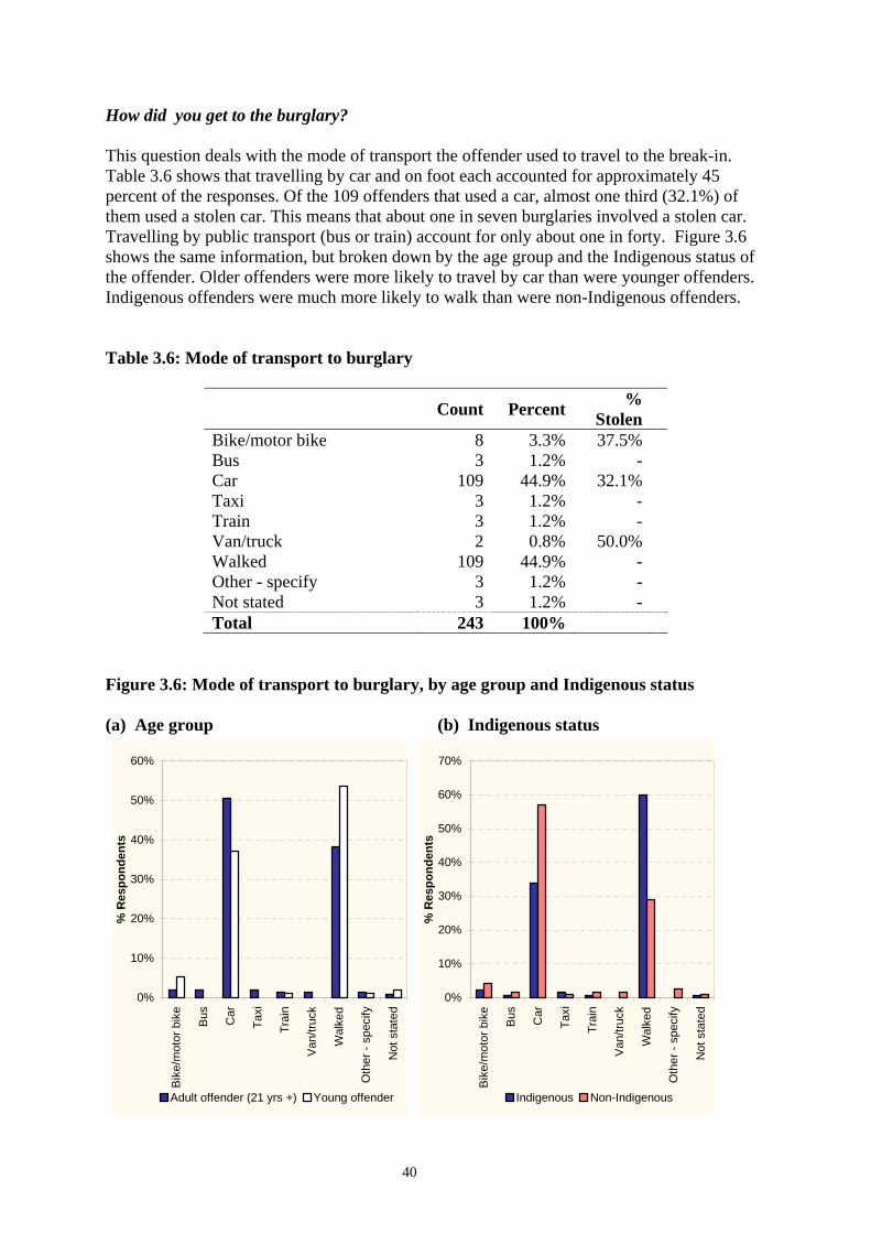
40

How did you get to the burglary? This question deals with the mode of transport the offender used to travel to the break-in. Table 3.6 shows that travelling by car and on foot each accounted for approximately 45 percent of the responses. Of the 109 offenders that used a car, almost one third (32.1%) of them used a stolen car. This means that about one in seven burglaries involved a stolen car. Travelling by public transport (bus or train) account for only about one in forty. Figure 3.6 shows the same information, but broken down by the age group and the Indigenous status of the offender. Older offenders were more likely to travel by car than were younger offenders. Indigenous offenders were much more likely to walk than were non-Indigenous offenders. Table 3.6: Mode of transport to burglary

Count Percent % Stolen

Bike/motor bike 8 3.3% 37.5% Bus 3 1.2% - Car 109 44.9% 32.1% Taxi 3 1.2% - Train 3 1.2% - Van/truck 2 0.8% 50.0% Walked 109 44.9% - Other - specify 3 1.2% - Not stated 3 1.2% - Total 243 100%

Figure 3.6: Mode of transport to burglary, by age group and Indigenous status (a) Age group (b) Indigenous status

0%

10%

20%

30%

40%

50%

60%

Bik

e/m

otor

bik

e

Bus Car

Taxi

Trai

n

Van

/truc

k

Wal

ked

Oth

er -

spec

ify

Not

sta

ted

% R

espo

nden

ts


0%

10%

20%

30%

40%

50%

60%

70%

Bik

e/m

otor

bik

e

Bus Car

Taxi

Trai

n

Van

/truc

k

Wal

ked

Oth

er -

spec

ify

Not

sta

ted

% R

espo

nden

ts


41

Did you leave the place in the same way that you got there? This question deals with whether or not the offender used the same mode of transport to leave the break-in. Table 3.7 shows that most offenders (83.1%) used the same mode of transport. Figure 3.7 shows the same information, but broken down by the age group and the Indigenous status of the offender. Younger offenders were slightly more likely to leave in the same way than older offenders. Indigenous and non-Indigenous offenders were about equally likely to leave in the same way. Table 3.7: Same mode of transport from burglary


Figure 3.7: Same mode of transport from burglary, by age group and Indigenous status (a) Age group (b) Indigenous status

0%

10%

20%

30%

40%

50%

60%

70%

80%

90%

Yes No

Not

sta

ted

% R

espo

nden

ts


0%

10%

20%

30%

40%

50%

60%

70%

80%

90%

Yes No

Not

sta

ted

% R

espo

nden

ts


42

Where did you go after the break-in? This question deals with where the offender went immediately after the break-in. Table 3.8 shows that almost 30 percent went home, 23.9 percent went to a friend’s house and 15.6 percent went to dealer, fence or pawnbroker. Only 2.5 percent went to do another break-in and only 3.7 percent got caught. Figure 3.8 shows the same information, but broken down by the age group and the Indigenous status of the offender. Overall, Figures 3.8a and 3.8b show no marked differences in the percentages of the places offenders went to immediately after the offence, both for age group and by Indigenous status. Table 3.8: Where went after

Count Percent Home 72 29.6% A family member’s house 14 5.8% A friend's house 58 23.9% Got caught 9 3.7% To another break-in 6 2.5% Dealer/fence/pawnbroker 38 15.6% Not stated 17 7.0% Total 243 100%

Figure 3.8: Where went after, by age group and Indigenous status (a) Age group (b) Indigenous status

0%

5%

10%

15%

20%

25%

30%

35%

40%

45%

A fri

end'

sho

use

Hom

e

To a

noth

erbr

eaki

n

Oth

er -

spec

ify

Not

sta

ted

% R

espo

nden

ts


0%

5%

10%

15%

20%

25%

30%

35%

40%

45%

A fri

end'

sho

use

Hom

e

To a

noth

erbr

eaki

n

Oth

er -

spec

ify

Not

sta

ted

% R

espo

nden

ts


43

What was taken from the break-in?(Portability) This question asked the respondent to choose from a list of 15 items any that described what was taken from the break-in. What may be relevant here is how the portability of the items relate to issues, such as the mode of transport chosen and the distance travelled. Therefore, the types of items were classified as large (TV, stereo, VCR, computers) or small (all other item types). Table 3.9 shows that about two thirds of burglaries involved taking only smaller items. Table 3.10 shows the portability, broken down by the transport mode used. Offenders who took large items were more likely to use a car and offenders who took only small items were more likely to walk. Table 3.9: Portability of items taken

Count Percent Large Items 83 34.2% No Large Items 160 65.8% Total 243 100%

Table 3.10: Portability of items taken, by transport mode to burglary

Large Not Large

Bike/motor bike 3.6% 3.1% Bus 2.4% 0.6% Car 50.6% 41.9% Not stated 1.2% 1.3% Other - specify 1.2% 1.3% Taxi 1.2% 1.3% Train 2.4% 0.6% Van/truck 1.2% 0.6% Walked 36.1% 49.4% Total 100% 100%

44

Distance Analysis The next series of results concentrates on the distance aspect of the journey to burglary and the journey from burglary. Distances will be examine with respect to distance from home and from where the offender slept the night before, transport modes, storage, portability of items stolen, time of day and drug use. Distance from home This question deals with the distance from the offender’s home to the break-in site. Table 3.11 shows that 62.6 percent of the burglaries were more than three kilometres away and 15.2 percent were within one kilometre. Figure 3.9 shows the same information, but broken down by the age group and the Indigenous status of the offender. Older offenders were more likely to travel larger distances than were younger offenders. Indigenous offenders were more likely to travel shorter distances than were non-Indigenous offenders. Table 3.11: Distance from home

Count Percent Less than 1km 37 15.2% Between 1 and 2km 28 11.5% Between 2 and 3km 20 8.2% More than 3km 152 62.6% Not stated 6 2.5% Total 243 100%

Figure 3.9: Distance from home, by age group and Indigenous status (a) Age group (b) Indigenous status

0%

10%

20%

30%

40%

50%

60%

70%

Less

than

1km

Bet

wee

n 1

and

2km

Bet

wee

n 2

and

3km

Mor

e th

an 3

km

Not

sta

ted

% R

espo

nden

ts


0%

10%

20%

30%

40%

50%

60%

70%

80%

Less

than

1km

Bet

wee

n 1

and

2km

Bet

wee

n 2

and

3km

Mor

e th

an 3

km

Not

sta

ted

% R

espo

nden

ts


45

Distance from place slept night before This question deals with the distance travelled from the place the offender slept the night before the break-in. Table 3.12 shows that 63.2 percent of burglars travelled more than three kilometres, but only 5.3 percent travelled less than one kilometre. Table 3.12: Distance, by place slept night before


Distance, by mode of transport to burglary Figure 3.10 shows the distance travelled, by mode of transport. When vehicles were used, the burglary was more than three kilometres away in of 80 percent of the burglaries. When the offender walked, just over 30 percent of the burglaries were less than one kilometre away, but almost 40 percent were more than three kilometres away. Figure 3.10: Distance, by mode of transport to burglary

0%10%20%30%40%50%60%70%80%90%

Vehicle Public transport Other/Not stated Walked

% R

espo

nden

ts

Less than 1km Between 1 and 2km Between 2 and 3kmMore than 3km Not stated

46

Storage distance from the break-in These results are based on the question that asked about the distance from the site of the burglary to the site of storage of the items taken, if they were in fact stored. Of the 243 respondents, 42 said they stored items, 186 said they did not and 15 did not state either way. Table 3.13 shows the distances to the storage site for those 42 burglaries. Almost two thirds stored the items more than three kilometres away. Table 3.13: Storage distance


Distance, by portability of items taken Table 3.14 shows how the distance travelled is related to the portability of the items taken. Two thirds (66.3%) of the burglars who took large items travelled more than three kilometres, while slightly less of the burglars who took only small items travelled that far. The portability does not show a marked effect on the distance travelled. Table 3.14: Distance, by portability of items taken

Large Not Large

Less than 1km 15.7% 15.0% Between 1 and 2km 10.8% 11.9% Between 2 and 3km 4.8% 10.0% More than 3km 66.3% 60.6% Not stated 2.4% 2.5% Total 100% 100%

47

Distance from home, by time of day Figure 3.11 shows the distance travelled from the offender’s home to the burglary site, for each time period of the day. During the morning period distances of less than one kilometre make up a larger proportion of the burglaries than they do in other time periods, and during the night-time period they make up a smaller proportion. Distances of over three kilometres make up a larger proportion of the burglaries in the night-time period than they do in other time periods. Comparing ‘day’ (6am to 6pm) with ‘night’ (6pm to 6am) shows similar results: journeys less than one kilometre make up a greater proportion of burglaries in the day and journeys over three kilometres make up a greater proportion of burglaries in the night. Figure 3.11: Distance from home, by time of day

0%

10%

20%

30%

40%

50%

60%

70%

Morning(6am-12pm)

Afternoon(12pm-6pm)

Evening(6pm-12am)

Night-time(12am-6am)

% R

espo

nden

ts

Less than 1km Between 1 and 2km Between 2 and 3km More than 3km Distance from home, by drug use Figure 3.12 shows the distance travelled from the offender’s home to the burglary site, by the frequency and severity of the burglar’s drug use. Burglars with no frequent and/or no severe drug use travel less distances to burgle than do burglars with frequent and/or severe drug use. This supports the idea that a burglar with frequent or severe drug habits would have a more frequent and more urgent need to get drugs. Thus, they may be more willing to exert more effort in travelling to an appropriate target. Figure 3.12: Distance from home, by drug use

0%

10%

20%

30%

40%

50%

60%

70%

Frequent &/or severe illicit drug use No frequent &/or severe illicit drug

% R

espo

nden

ts

Less than 1km Between 1 and 2km Between 2 and 3km More than 3km

48

REFERENCES Brantingham, Paul and Brantingham, Patricia (eds) (1984), Environmental criminology. Prospect Heights: Waveland Press. Brantingham, Paul and Brantingham, Patricia (1984), Patterns in crime. New York: Macmillan. Clare, J., Fernandez, J. and Morgan, F., (forthcoming), Burglary target choice. Clarke, R.V. and Cornish, D.B. (1986), The reasoning criminal. New York: Springer-Verlag. Cohen, L.E. and Felson, M. (1979), ‘Social change and crime rate trends: a routine activities approach’, American Sociological Review, 44: 588-608. Ferrante, A. and Clare, J. (2006), “Known” burglars and the stolen goods market in Western Australia. (Research report to the Office of Crime Prevention, Western Australia.) Ratcliffe, J.H. and McCullagh, M.J. (1998), Aoristic crime analysis. International Journal of Geographic Information Science 12: 751-764. Wiles, P. and Costello, A. (2000), The ‘road to nowhere’: the evidence for travelling criminals. (Home Office Research Study No. 207.) London: Home Office.

49

Appendix A – Caveats on WA Police Data The following caveats relate to the release and use of police data presented in this document, where applicable:

1. The Data/Information was supplied courtesy of the WA Police Service and was sourced from the Service’s Offence Information System / Frontline Incident Management System.

2. The Data/Information is provisional and may be subject to revision.

3. Reported offences are selected offences reported to or becoming known to police, and resulting in the submission of an offence/incident report in the Offence Information System/Frontline Incident Management System. These exclude offences against public order, such as disorderly conduct and offences against the Firearms Act, Liquor Licensing Act and a number of other offences against the statute laws of this State and the Commonwealth.

4. The number of reported offences for a period comprises all offences reported during that period and may include offences committed during earlier periods. Therefore the reporting of historical offences may inflate the number of reported offences for a given period.

5. Offence classifications may alter between or during periods due to changes in legislation, administrative recording practices and system coding. Similarly, locality boundaries may also change. Accordingly, time series may be broken over time.

6. From late 2002, a number of factors have affected victim reporting and police recording of offence and clearance statistics. For example: (a) The offence category of ‘manslaughter’ includes some offences resulting from driving incidents, which have previously been included in the category of ‘driving causing death’; (b) Recording issues associated with the offence category of ‘assault police officer’ have resulted in a number of these offences being recorded in the categories of ‘aggravated assault’ and ‘non aggravated assault’; (c) Policy changes in some sectors of the finance industry and recording issues associated with the offence category of ‘fraud’ have had an impact on the number of reported offences; (d) Recording issues and reporting practices by some Government agencies, local government authorities and private enterprise associated with the offence category of ‘graffiti’ have resulted in a decrease in the number of reported offences; (e) Definitional, coding and processing changes associated with the introduction of the Frontline Incident Management System have had an impact on some data.

Accordingly, caution should be exercised when interpreting and using offence and clearance statistics from late 2002, especially when comparing those statistics with earlier periods. For example, any variation may not necessarily reflect an actual increase or decrease in the incidence of an offence type (or in total offence numbers), but rather variations resulting from reporting and recording changes. The clearance of offences is similarly impacted upon.

7. An offence is deemed to be cleared where a satisfactory result has been achieved or where, for some substantial reason, police investigations cannot be continued. This includes: offender(s) processed by arrest, summons, Juvenile Justice Team referral or juvenile caution; the offender has died; the offender is in another jurisdiction and extradition is not desired or available; there is a statute bar to proceedings where an offender is underage or is subject to diplomatic immunity; admittance to a psychiatric facility; false or mistaken reports; civil action recommended.

8. The number of offences cleared for a period comprises all offences for which the clearance was recorded during that period. Due to the nature and length of investigations, the number of offences cleared during a period may include offences reported prior to that period. Clearances are also attributed according to the locality in which the offence occurred, not the locality at which the offence was cleared.

9. Aboriginality and indigenous status data is derived from the WA Police Service Identity Code field for Ethnic Appearance. This field is completed on the basis of the attending police officer’s subjective assessment of the person’s appearance, and is recorded for operational purposes only. Care should be exercised in the interpretation of these statistics, as a subjective assessment means it is possible that a person attributed to a particular group may not belong to that group.

Suburban Travel Patterns in Burglary

Documents

Transcript of Suburban Travel Patterns in Burglary