Subir Sachdev and T. Senthil- Zero temperature phase transitions in quantum Heisenberg ferromagnets
45
a r X i v : c o n d m a t / 9 6 0 2 0 2 8 6 F e b 9 6 Zero temperature phase transitions in quantum Heisenberg ferromagnets Subir Sachdev and T. Senthil Department of Physics, P.O.Box 208120, Yale University, New Haven, CT 06520-8120 (February 5, 1996) Abstract The purpose of this work is to understand the zero temperature phases, and the phase transitions, of Heisenberg spin systems which can have an extensive, spontaneous magnetic moment; this entails a study of quantum transitions with an order parameter which is also a non -abe lian conse rv ed charge. To this end, we introduce and study a new class of lattice models of quantum rotors. We compute their mean-field phase diagrams, and present continuum, quantum field-theoretic descriptions of their low energy properties in different regimes. We argue that, in spatial dimension d = 1, the phase transitions in itinerant Fermi systems are in the same universality class as the corresponding transitions in certain rotor models. We discuss implications of our results for itineran t fermions systems in highe r d, and for other physical systems. Typeset using REVT E X 1 Annals of Physics 251, 76 (1996)
Transcript of Subir Sachdev and T. Senthil- Zero temperature phase transitions in quantum Heisenberg ferromagnets
8/3/2019 Subir Sachdev and T. Senthil- Zero temperature phase transitions in quantum Heisenberg ferromagnets
http://slidepdf.com/reader/full/subir-sachdev-and-t-senthil-zero-temperature-phase-transitions-in-quantum 1/45
a r X i v : c o n d - m a t / 9 6 0 2 0 2 8
6 F e b 9 6
Zero temperature phase transitions in quantum Heisenberg
ferromagnets
Subir Sachdev and T. Senthil
Department of Physics, P.O.Box 208120, Yale University, New Haven, CT 06520-8120 (February 5, 1996)
Abstract
The purpose of this work is to understand the zero temperature phases, and
the phase transitions, of Heisenberg spin systems which can have an extensive,
spontaneous magnetic moment; this entails a study of quantum transitions
with an order parameter which is also a non-abelian conserved charge. To
this end, we introduce and study a new class of lattice models of quantum
rotors. We compute their mean-field phase diagrams, and present continuum,
quantum field-theoretic descriptions of their low energy properties in different
regimes. We argue that, in spatial dimension d = 1, the phase transitions in
itinerant Fermi systems are in the same universality class as the corresponding
transitions in certain rotor models. We discuss implications of our results for
itinerant fermions systems in higher d, and for other physical systems.
Typeset using REVTEX
1
Annals of Physics 251, 76 (1996)
8/3/2019 Subir Sachdev and T. Senthil- Zero temperature phase transitions in quantum Heisenberg ferromagnets
http://slidepdf.com/reader/full/subir-sachdev-and-t-senthil-zero-temperature-phase-transitions-in-quantum 2/45
I. INTRODUCTION
Despite the great deal of attention lavished recently on magnetic quantum critical phe-nomena, relatively little work has been done on systems in which one of the phases hasan extensive, spatially averaged, magnetic moment. In fact, the simple Stoner mean-field
theory [1] of the zero temperature transition from an unpolarized Fermi liquid to a ferro-magnetic phase is an example of such a study, and is probably also the earliest theory of a quantum phase transition in any system. What makes such phases, and the transitionsbetween them, interesting is that the order parameter is also a conserved charge; in sys-tems with a Heisenberg O(3) symmetry this is expected to lead to strong constraints on thecritical field theories [2]. As we will discuss briefly below, a number of recent experimentshave studied systems in which the quantum fluctuations of a ferromagnetic order parameterappear to play a central role. This emphasizes the need for a more complete theoreticalunderstanding of quantum transitions into such phases. In this paper, we will introducewhat we believe are the simplest theoretical models which display phases and phase transi-tions with these properties. The degrees of freedom of these models are purely bosonic and
consist of quantum rotors on the sites of a lattice. We will also present a fairly completetheory of the universal properties of the phases and phase transitions in these models, atleast in spatial dimensions d > 1. Our quantum rotor models completely neglect chargedand fermionic excitations and can therefore probably be applied directly only to insulatingferromagnets. However, in d = 1, we will argue that the critical behaviors of transitions inmetallic, fermionic systems are identical to those of the corresponding transitions in certainquantum rotor models.
We now describe the theoretical and experimental motivation behind our work:(i ) The Stoner mean field theory of ferromagnetism [1] in electronic systems in fact con-tains two transitions: one from an unpolarized Fermi liquid to a partially polarized itinerant
ferromagnet (which has received some recent experimental attention [3]), and the secondfrom the partially polarized to the saturated ferromagnet. A theory of fluctuations near thefirst critical point has been proposed [4,5] but many basic questions remain unanswered [2],especially on the ordered side [6] (there is no proposed theory for the second transition,although we will outline one in this paper). It seems useful to examine some these issuesin the simpler context of insulating ferromagnets. Indeed, as we have noted, we shall arguebelow that in d = 1, certain insulating and itinerant systems have phase transitions that arein the same universality class.
(ii ) Many of the phases we expect to find in our model also exist in experimental com-pounds that realize the so-called “singlet-triplet” model [7]. These compounds were studied
many years ago [8] with a primary focus on finite temperature, classical phase transitions; wehope that our study will stimulate a re-examination of these systems to search for quantumphase transitions(iii ) All of the phases expected in our model (phases A-D in Section I B below), occur inthe La1−xSrxMnO3 compounds [9]. These, and related compounds, have seen a great dealof recent interest for their technologically important “colossal magnetoresistance”.(iv ) Recent NMR experiments by Barrett et. al. [11] have studied the magnetization of aquantum Hall system as a function of both filling factor, ν , and temperature, T , near ν = 1.
2
8/3/2019 Subir Sachdev and T. Senthil- Zero temperature phase transitions in quantum Heisenberg ferromagnets
http://slidepdf.com/reader/full/subir-sachdev-and-t-senthil-zero-temperature-phase-transitions-in-quantum 3/45
The T = 0 state at ν = 1 is a fully polarized ferromagnet [12–15] and its finite temperatureproperties have been studied from a field-theoretic point of view [16]. More interesting forour purposes here is the physics away from ν = 1: Brey et. al. have proposed a variationalground state consisting of a crystal of “skyrmions”; this state has magnetic order that iscanted [18], i.e. in addition to a ferromagnet moment, the system has magnetic order (with
a vanishing spatially averaged moment) in the plane perpendicular to the average moment.A phase with just this structure will appear in our analysis, along with a quantum-criticalpoint between a ferromagnetic and a canted phase. Although our microscopic models arequite different from those appropriate for the quantum Hall system, we expect the insightsand possibly some universal features of our results to be applicable to the latter.
There has also been some interesting recent work on the effects of randomness on itinerantferromagnets [19]. This paper shall focus exclusively on clean ferromagnets, and the study of the effects of randomness on the models of this paper remains an interesting open problem;we shall make a few remarks on this in Section VII 3
In the following subsection we will introduce one of the models studied in this paper,followed by a brief description of its phases in Section I B. Section I will conclude with an
outline of the remainder of the paper.
A. The Model
We introduce the quantum rotor model which shall be the main focus of the paper;extensions to related models will be considered later in the body of the paper. On each sitei of a regular lattice in d dimensions there is a rotor whose configuration space is the surfaceof a sphere, described by the 3-component unit vector niµ (µ = 1, 2, 3 and
µ n2
iµ = 1); thecaret denotes that it is a quantum operator. The canonically conjugate angular momentaare the Liµ, and these degrees of freedom obey the commutation relations (dropping the site
index as all operators at different sites commute)
[nµ, nν ] = 0 ; [Lµ, Lν ] = iµνλLλ ; [Lµ, nν ] = iµνλnλ (1.1)
As an operator on wavefunctions in the nµ configuration space, Lµ is given by
Lµ = −iµνλnν ∂
∂nλ(1.2)
We will be interested primarily in the properties of the Hamiltonian
H =g
2i
L2iµ + α
L2iµ2−
<ij>
J niµn jµ + K LiµL jµ + M
niµL jµ + n jµLiµ
(1.3)
where there is an implied summation over repeated µ indices, and < ij > is the sum overnearest neighbors, and the couplings g, α, J , K , M are all positive. All previous analysesof quantum rotor models [20–23] have focussed exclusively on the case K = M = 0, and thenovelty of our results arises primarily from nonzero values of the new K, M couplings. Acrucial property of H is that the 3 charges
3
8/3/2019 Subir Sachdev and T. Senthil- Zero temperature phase transitions in quantum Heisenberg ferromagnets
http://slidepdf.com/reader/full/subir-sachdev-and-t-senthil-zero-temperature-phase-transitions-in-quantum 4/45
Qµ =i
Liµ (1.4)
commute with it, and are therefore conserved. Indeed, H is the most general Hamiltonianwith bilinear, nearest neighbor couplings between the nµ and Lµ operators, consistent with
conservation of theˆ
Qµ. We have also included a single quartic term, with coefficient gα,but its role is merely to suppress the contributions of unimportant high energy states.Discrete symmetries of H will also be important in our considerations. Time-reversal
symmetry, T is realized by the transformations
T : Lµ → −Lµ nµ → −nµ (1.5)
Notice that the commutators (1.1) change sign under T , consistent with it being an anti-unitary transformation. All the models considered in this paper will have T as a symmetry.For the special case M = 0, we also have the additional inversion symmetry P :
P : Lµ
→Lµ nµ
→ −nµ (1.6)
The presence of P will make the properties of the M = 0 system somewhat different fromthe M = 0 case. We will see later that P is related to a discrete spatial symmetry of theunderlying spin system that H models.
The utility of H does not lie in the possibility of finding an experimental system whichmay be explicitly modeled by it. Rather, we will find that it provides a particularly simpleand appealing description of quantum phases and phase transitions with a conserved orderparameter in a system with a non-abelian symmetry. Further, we will focus primarily onuniversal properties of H , which are dependent only on global symmetries of the states;these properties are expected to be quite general and should apply also to other modelswith the same symmetries, including those containing ordinary Heisenberg spins.
To help the reader develop some intuition on the possibly unfamiliar degrees of freedom inH , we consider in Appendix A a general double-layer Heisenberg spin model [24] containingboth inter- and intra-layer exchange interactions. We show that, under suitable conditions,there is a fairly explicit mapping of the double layer model to the quantum rotor HamiltonianH . Under this mapping we find that each pair of adjacent spins on the two layers behaveslike a single quantum rotor. In particular Lµ ∼ S aµ + S bµ and nµ ∼ S aµ − S bµ where a, b are
the two layers and the S µ are Heisenberg spins. Notice also that P is a layer-interchangesymmetry.
Before turning to a description of the ground state of H , it is useful to draw a parallel toanother model which has seen a great deal of recent interest—the boson Hubbard model [ 25].
The latter model has a single conserved charge, N b the total boson number, associated withan abelian global U (1) symmetry. In contrast, the quantum rotor model H has the 3 chargesQµ, and a non-abelian global O(3) symmetry. As we will see, the non-abelian symmetry
plays a key role and is primarily responsible for the significant differences between H andthe boson Hubbard model. It is also useful to discuss a term-by-term mapping betweenH and the boson Hubbard model. The terms proportional to g in H are analogous to theon-site Hubbard repulsion in the boson model. The latter model also has an on-site chemicalpotential term which couples linearly to N B, but such a term is prohibited by symmetry in
4
8/3/2019 Subir Sachdev and T. Senthil- Zero temperature phase transitions in quantum Heisenberg ferromagnets
http://slidepdf.com/reader/full/subir-sachdev-and-t-senthil-zero-temperature-phase-transitions-in-quantum 5/45
the non-abelian rotor model. The J term in H has an effect similar to the boson hoppingterm, while the K term is like a nearest-neighbor boson density-density interaction. Thereis no analog of the M term in the boson Hubbard model.
B. Zero temperature phases of H
We show in Fig 1 the zero temperature (T ) phase diagram of H in the K, J plane at fixedg, α, and M . This phase diagram was obtained using a mean-field theory which becomesin exact in the limit of large spatial dimensionality (d); however, the topology and generalfeatures are expected to be valid for all d > 1. The d = 1 case will be discussed separatelylater in the paper; in the following discussion we will assume d > 1. We will also assumebelow that P symmetry is absent, unless otherwise noted. Throughout this paper we willrestrict consideration to parameters for which the ground state of H are translationallyinvariant ground states—this will require that M not be too large.
There are four distinct classes of phases:
(A) Quantum Paramagnet:This is a featureless spin singlet and there is a gap to all excitations. The O(3) symmetry
remains unbroken, as
nµ =
Lµ
= 0. (1.7)
Clearly this phase will always occur when g is much bigger than all the other couplings.(B)Quantized Ferromagnets:
These are ordinary ferromagnets in which the total moment of the ground state is quan-tized in integer multiples of the number of quantum rotors (extensions of H in which thequantization is in half-integral multiples will be considered later in this paper). The fer-
romagnetic order parameter chooses a direction in spin space (say, z), but the symmetryof rotations about this direction remains unbroken. The ground state therefore has theexpectation values
Lz
= integer = 0 ; nz = 0 (1.8)
The value of nz is not quantized and varies continuously as K , J , and M are varied; for thesystem with P symmetry (M = 0) we will have nz = 0 in this phase. If we consider eachquantum rotor as an effective degree of freedom representing a set of underlying Heisenbergspins (as in the double-layer model of Appendix A), then nz determines the manner inwhich the quantized moment is distributed among the constituent spins. The low-lying
excitation of these phases is a gapless, spin-wave mode whose frequency ω ∼ k2 where k isthe wavevector of the excitation.
That these phases occur is seen as follows: First consider the line J = 0, M = 0. For verysmall K , it is clear that the ground state is a quantum paramagnet.As K is increased, it iseasy to convince oneself (by an explicit calculation) that a series of quantized ferromagnet
phases with increasing values of
Lz
= integer get stabilized. Further in this simple limit
the exact ground state in each one of these phases is just a state in which each site is putin the same eigenstate of L2 and Lz. There is a finite energy cost to change the value of
5
8/3/2019 Subir Sachdev and T. Senthil- Zero temperature phase transitions in quantum Heisenberg ferromagnets
http://slidepdf.com/reader/full/subir-sachdev-and-t-senthil-zero-temperature-phase-transitions-in-quantum 6/45
L2 at any site. Now consider moving away from this limit by introducing small non-zerovalues of J and M . These terms vanish in the subspace of states with a constant value of L2
i so we need to consider excitations to states which involve changing the value of L2i at
some site. As mentioned above such states are separated from the ground state by a gap.Consequently, though the new ground state is no longer the same as at J = 0, M = 0, it’s
quantum numbers , in particular the value of Qz =
i Liz, are unchanged.The stability of the quantized ferromagnet phases up to finite values of J and M implies the existence of direct transitions between them which is naturally first order. In general a non-zero valueof M will also lead to a non-zero value of nz.
All of this should remind the reader of the Mott-insulating phases of the boson Hubbardmodel [25]. In the latter, the boson number, nb, is quantized in integers, which is the analogof the conserved angular momentum Lµ of the present model. However, the properties of the Mott phases are quite similar for all values of nb, including nb = 0. In contrast, for
the O(3) rotor model, the case
Lz
= 0 (the quantum paramagnet, which has no broken
symmetry and a gap to all excitations) is quite different from
Lz
= integer = 0 cases
(the quantized ferromagnets, which have a broken symmetry and associated gapless spin-wave excitations). As we argued above and as shown in Fig 1, the lobes of the quantizedferromagnets and the quantum paramagnet are separated by first-order transitions, whilethere were no such transitions in the phase diagram for the boson Hubbard model in Ref [ 25];this is an artifact of the absence of off-site boson attraction terms analogous to the K termin Ref [25], and is not an intrinsic difference between the abelian and non-abelian cases.(C) Neel Ordered Phase:
In this phase we have
nµ = 0, while
Lµ
= 0. (1.9)
This occurs when J is much bigger than all other couplings. We refer to it as the Neel
phase because the spins in the bilayer model are oriented in opposite directions in the twolayers. More generally, this represents any phase in which the spin-ordering is defined by asingle vector field (nµ) and which has no net ferromagnetic moment. There are 2 low-lyingspin-wave modes, but they now have a linear dispersion ω ∼ k [26]. The order parametercondensate nµ does not have a quantized value and varies continuously with changes inthe couplings.
From the perspective of classical statistical mechanics, the existence of this Neel phase israther surprising. Note that there is a linear coupling M Liµniµ in H between the nµ and Lµ
fields. In a classical system, such a coupling would imply that a non-zero condensate of Lµ
must necessarily accompany any condensate in nµ. The presence of a phase here, in which
Lµ
= 0 despite nµ = 0, is a consequence of the quantum mechanics of the conservedfield Lµ.(D) Canted Phase:
Now both fields have a condensate:
nµ = 0 and
Lµ
= 0. (1.10)
The magnitudes of, and relative angle between, the condensates can all take arbitrarilyvalues, which vary continuously as the couplings change; however if P is a symmetry (if
6
8/3/2019 Subir Sachdev and T. Senthil- Zero temperature phase transitions in quantum Heisenberg ferromagnets
http://slidepdf.com/reader/full/subir-sachdev-and-t-senthil-zero-temperature-phase-transitions-in-quantum 7/45
M = 0) then nµ is always orthogonal to
Lµ
. The O(3) symmetry of H is completely
broken as it takes two vectors to specify the orientation of the condensate. In the bilayermodel, the spins in the two layers are oriented in two non-collinear directions, such thatthere is a net ferromagnetic moment. The low lying excitations of this phase consist of 2spin wave modes, one with ω
∼k, while the other has ω
∼k2. This phase is the analog
of the superfluid phase in the boson Hubbard model. In the latter model the conservednumber density has an arbitrary, continuously varying value and there is long range orderin the conjugate phase variable; similarly here the conserved
Lµ
has an arbitrary value
and the conjugate nµ field has a definite orientation.At this point, it is useful to observe a parallel between the phases of the quantum rotor
model and those of a ferromagnet Fermi liquid. This parallel is rather crude for d > 1, but,as we will see in Secs VI and VII, it can be made fairly explicit in d = 1 where we believethat the universality classes of the transitions in the rotor model and the Fermi liquid areidentical. The quantized ferromagnetic phases B are the analogs of the fully polarized phaseof the Fermi liquid in which the spins of all electrons are parallel. The canted phase D hasa continuously varying ground state polarization, as in a partially polarized Fermi liquid.Finally the Neel phase C is similar to an unpolarized Fermi liquid in that both have no netmagnetization and exhibit gapless spin excitations.
Finally, we point out an interesting relationship between phases with a non-quantizedvalue of the average magnetization (as in phase D of the rotor model), and phases withvanishing average magnetization (phases A and C). Notice that, in both the Fermi liquidand the quantum rotor model, it is possible to have a continuous transition between suchphases. However, in both cases, such a transition only occurs when the phase with vanishingmagnetization has gapless spin excitations; in phase C of the rotor model we have the gaplessspin waves associated with the Neel long range order, while in the unpolarized Fermi liquidwe have gapless spin carrying fermionic quasiparticles. Phase A of the rotor model has
no gapless excitations, but notice that there is no continuous transition between it andthe partially polarized canted phase D. We believe this feature to be a general principle:continuous zero temperature transitions in which there is an onset in the mean value of a
non-abelian conserved charge only occur from phases which have gapless excitations.
The outline of the remainder of the paper is as follows. We will begin in Section II bydiscussing the mean field theory which produced the phases described above. In Section IIIwe will perform a small fluctuation analysis of the low-lying excitations of the phases. Wewill turn our attention to the quantum phase transitions in d > 1 in Section IV, focusingmainly on the transition between phases C and D in Section IV A, and that between phasesB and D in Section IV B. In Section V we shall consider an extension of the basic rotor model(1.3): each rotor will have a ‘magnetic monopole’ at the origin of n space, which causes the
angular momentum of each rotor to always be non-zero. We will turn our attention to theimportant and distinct physics in d = 1 in Section VI. We will conclude in Section VII byplacing our results in the context of earlier work and discuss future directions for research.Some ancillary results are in 5 appendices: we note especially Appendix D, which containsnew universal scaling functions of the dilute Bose gas, a model which turns out to play acentral role in our analysis.
7
8/3/2019 Subir Sachdev and T. Senthil- Zero temperature phase transitions in quantum Heisenberg ferromagnets
http://slidepdf.com/reader/full/subir-sachdev-and-t-senthil-zero-temperature-phase-transitions-in-quantum 8/45
II. MEAN FIELD THEORY
In this section we will describe the mean-field theory in which the phase diagram of Fig 1was obtained. The mean-field results become exact in the limit of large spatial dimensional-ity, d. Rather than explicitly discussing the structure of the large d limit, we choose instead
a more physical discussion. We postulate on every site a single-site mean field Hamiltonian
H mf =g
2
L2
µ + α
L2µ
2− N µnµ − hµLµ (2.1)
which is a function of the variational c-number local fields N µ and hµ. These fields are deter-
mined at T = 0 by minimizing the expectation value of H in the ground state wavefunctionof H mf . The mean-field ground state energy of H is
E mf = E 0 − JZ
2nµ20 − KZ
2
Lµ
20− MZ nµ0
Lµ
0
+ N µ nµ0 + hµ
Lµ
0
(2.2)
where E 0 is the ground state energy of the H mf , all expectation values are in the groundstate wavefunction of H mf , and Z is the co-ordination number of the lattice. We now haveto minimize the value of E mf over variations in hµ and N µ. This was carried out numericallyfor a characteristic set of values of the coupling constants. Stability required that the cou-pling M not be too large. Further details may be found in Appendix B. Here we describethe behavior of the local effective fields hµ, N µ in the various phases:(A) Quantum Paramagnet:
This phase has no net effective fields N µ = 0, hµ = 0.(B) Quantized Ferromagnets:
We now have N z = 0 and hz = 0 with all other components zero. The values of N z and hz
both vary continuously as the parameters are changed. Nevertheless, the value of Lz re-
mains pinned at a fixed non-zero integer. This is clearly possible only because Lµ commutes
with H and H mf , and Lz is therefore a good quantum number.(C) Neel Ordered Phase:
Like phase B, this phase has N z = 0 and hz = 0 with all other components zero, andthe values of N z and hz both vary continuously as the parameters are changed. However
Lz
= 0; it is now quantized at an integer value which happens to be zero. As a result,
there is no net ferromagnetic moment in this phase. This unusual relationship between anorder parameter
Lµ
, and its conjugate field hµ, is clearly a special property of the interplay
between quantum mechanics and conservation laws, and cannot exist in classical statisticalmechanics systems.
(D) Canted Phase:Now both hµ and N µ are non-zero, and take smoothly varying values with no special con-
straints, as do their conjugate fields nµ and Lµ. In systems with P a good symmetry(M = 0), we have
µ hµN µ = 0.
8
8/3/2019 Subir Sachdev and T. Senthil- Zero temperature phase transitions in quantum Heisenberg ferromagnets
http://slidepdf.com/reader/full/subir-sachdev-and-t-senthil-zero-temperature-phase-transitions-in-quantum 9/45
III. STRUCTURE OF THE PHASES
The quantum paramagnet A is a featureless singlet phase with all correlations decayingexponentially in both space and imaginary time, and a gap to all excitations. The ferro-magnet phases B and the Neel phase C are conventional magnetically ordered phases and
hardly need further comment here. We describe below the long-wavelength, low energyquantum hydrodynamics of the canted phase D. We are implicitly assuming here, and in theremainder of this section that d > 1.
We will study the phase D by accessing it from the Neel phase C. We will analyzethe properties of D for small values of the uniform ferromagnetic moment; this leads to aconsiderable simplification in the analysis, but the form of the results are quite general andhold over the entire phase D—in a later section (Section IV B), we will also access phase Dfrom one of the quantized ferromagnetic phases B and obtain similar results.
We will use an imaginary time, Lagrangian based functional-integral point of view. Theanalysis begins by decoupling the inter-site interactions in H by the spacetime dependentHubbard Stratonovich fields N µ(x, τ ) and hµ(x, τ ); these fields act as dynamic local fields
similar to those in H mf (Eqn (2.1)). We can then set up the usual Trotter product decompo-sition of the quantum mechanics independently on each site: this yields the following localfunctional integral on each site (we are not displaying the inter-site terms involving the N µand hµ fields, as these will be considered later):
Z L =
Dnµδ(n2µ − 1)exp
− β
0dτ LL
LL =1
2g
∂nµ
∂τ − iµνλhν nλ
2
− nµN µ (3.1)
We have ignored, for simplicity, the contribution of the quartic α term in H. It is not possibleto evaluate Z L exactly; for time-independent source fields hµ, N µ, the evaluation of Z L is of course equivalent to the numerical diagonalization that was carried out in Section II. ForN µ = 0, however, we can obtain the following simple formula for the ground state energyE L = − limβ →∞(1/β )log Z L:
E L = Min [g( + 1)/2 − h] ; ≥ 0 , integer. (3.2)
The minimum is taken over the allowed values of , and we have again ignored the α term.Note that this is a highly non-analytic function of h: these non-analyticities are directly
responsible for the lobes of the quantized ferromagnetic phases B. In this section we willbegin by working in the region of parameters in which E L is minimized by = 0 (phases Aand C); in the vicinity of this region it is permissible to expand in powers of h. Inter-siteeffects will then eventually lead to a phase in which there is a net uniform moment (phaseD)— this moment will not be quantized and there will be appreciable fluctuations in themagnetic moment of each site (this is similar to fluctuations in particle number in a bosonsuperfluid phase). For simplicity we will first present the analysis for the case M = 0. Laterwe will indicate the modifications necessary when M = 0.
9
8/3/2019 Subir Sachdev and T. Senthil- Zero temperature phase transitions in quantum Heisenberg ferromagnets
http://slidepdf.com/reader/full/subir-sachdev-and-t-senthil-zero-temperature-phase-transitions-in-quantum 10/45
A. Model with P symmetry
Recall that P symmetry is present when M = 0.It is convenient to write an effective action functional in terms of the hµ and nµ fields:
the form of this functional can be guessed by symmetry and the usual Landau arguments:
Z =
DnµDhµ exp
−
ddx β
0dτ (L1 + L2)
L1 =K 12
∂nµ
∂τ − iµνλ(hν + H ν )nλ
2
+K 22
(nµ)2 +K 32
(hµ)2
+r12
h2µ +
u1
8(h2
µ)2
L2 =
r2
2 n2
µ + +
u2
8 (n2
µ)2
+
v1
2 (n2
µ)(h2
ν ) +
v2
2 (nµhµ)2
(3.3)
We have temporarily modified nµ from a fixed-length to a “soft- spin” field; this is merely forconvenience in the following discussion and not essential. Here H µ is an external magneticfield whose coupling to the fields is determined by gauge-invariance [2]. The reason forsplitting the Lagrangian into pieces L1, L2 will become clear below.
We can now look for static, spatially uniform, saddle points of L. This gives threedifferent types of solutions, corresponding to the phases A, C, and D (the absence of alength constraint on nµ is necessary to obtain all three saddle-points at tree level). Thevalues of the hµ and nµ fields at these saddle points are identical in form to those discussedfor these phases in Section II (with the reminder that we have temporarily specialized to
M = 0 so that P is a good symmetry). Note that there is no saddle point corresponding tothe B phases: this is clearly a consequence of ignoring the non-analytic behavior of h in Z L.
The low-lying excitation spectrum in the A, C, and D phases can now be determinedby an analysis of Gaussian fluctuations about the saddle points. While simple in principle,such an analysis is quite tedious and involved, especially in phase D. We will therefore notpresent it here; we present instead a more elegant approach in which the answer can beobtained with minimal effort.
Recall that an efficient method of obtaining the properties of the Neel phase is to usea non-linear sigma model in which the constraint n2
µ = 1 is imposed. This eliminates highenergy states from the Hilbert space associated with amplitude fluctuations, but does not
modify the low energy spectrum. We introduce here an extension to a hybrid sigma modelwhich allows also for the existence of the canted phase D. Notice from the mean- fieldsolutions in Sec II that the onset of the canted phase D is signaled by the appearance of an expectation value of hµ in a direction orthogonal to the mean direction of nµ, whilethe component of hµ parallel to nµ is zero in both the C (Neel) and D phases (note: thelast restriction on components of hµ and nµ parallel to each other requires P symmetryand M = 0). This suggests that the important fluctuations are the components of hµ
perpendicular to nµ, while fluctuations which change the dot product nµhµ are high energy
10
8/3/2019 Subir Sachdev and T. Senthil- Zero temperature phase transitions in quantum Heisenberg ferromagnets
http://slidepdf.com/reader/full/subir-sachdev-and-t-senthil-zero-temperature-phase-transitions-in-quantum 11/45
modes. So we define our hybrid sigma model by imposing the two rotationally invariantconstraints
nµnµ = 1 ; nµhµ = 0 (3.4)
With these constraints, the degrees of freedom have been reduced from the original 6 real
fields hµ, nµ to 4. Notice that while amplitude fluctuations of nµ have been eliminated, thosein the components of hµ orthogonal to nµ have not—this is the reason for the nomenclature‘hybrid’ above. As an immediate consequence of (3.4), all the terms in L2 either becomeconstants or modify couplings in L1, and L1 is the Lagrangian of the hybrid sigma model.
The Lagrangian L1 and the constraints (3.4) display, in principle, all three phases A,C, and D. We now move well away from phase A, assuming that nµ has a well developedexpectation value along the z direction. We then parametrize deviations from this state bythe following parametrization of the fields, which explicitly obeys the constraints (3.4):
n =
ψ + ψ∗
√2
,ψ − ψ∗
√2i
, (1 − 2|ψ|2)1/2
h =
φ + φ∗√
2,
φ − φ∗√2i
, − ψ∗φ + φ∗ψ
(1 − 2|ψ|2)1/2
. (3.5)
We have two complex fields ψ, φ, corresponding to the 4 degrees of freedom in the hybridsigma model. The field ψ represents oscillations of the nµ about its mean value: by definition,we will have ψ = 0 in all phases. The field φ measures the amplitude of hµ orthogonal tothe instantaneous value of nµ: we have φ = 0 in the Neel phase C, while φ = 0 in thecanted phase D. We now insert (3.5) into (3.3) and obtain at H = 0 the partition functionZ σ for our hybrid sigma model
Z σ = DφDφ
∗
Dψ
Dψ
∗1 − 2|ψ|2 exp−
d
d
x β
0 dτ (Lσ1 + Lσ2 + · · ·)Lσ1 = K 1
∂ψ
∂τ
2
+ K 1
φ∗
∂ψ
∂τ − φ
∂ψ∗
∂τ
+ K 2|ψ|2 + K 3|φ|2 + r4|φ|2
Lσ2 =u1
2|φ|4 +
K 12
∂ |ψ|2
∂τ
2
+ K 1|ψ|2
φ∗∂ψ
∂τ − φ
∂ψ∗
∂τ
+
K 22
|ψ|2
2
+K 32
|(ψ∗φ + ψφ∗)|2 +r42
(ψ∗φ + ψφ∗)2 (3.6)
where r4 = r1 + v1 − K 1. The Lagrangian Lσ1 (Lσ2) contains terms that are quadratic(quartic) in the fields. Note that, apart from the u1 term, all coupling constants in
Lσ2
are related to those in Lσ1: these constraints on the couplings encapsulate the rotationalinvariance of the underlying physics. The field ψ, which represents fluctuations of N µ aboutits average value has no “mass” term (a term with no gradients) in Lσ1; the constraints onthe couplings ensure that no such mass term is ever generated, and that the fluctuations of ψ remain gapless. This is exactly what is expected as the Neel order parameter is non-zeroin both the C and D phases. Finally, note that although we have only displayed Z σ forH = 0, the form of the coupling to a field H z in the z direction can be easily deduced fromthe gauge invariance arguments of Ref [2].
11
8/3/2019 Subir Sachdev and T. Senthil- Zero temperature phase transitions in quantum Heisenberg ferromagnets
http://slidepdf.com/reader/full/subir-sachdev-and-t-senthil-zero-temperature-phase-transitions-in-quantum 12/45
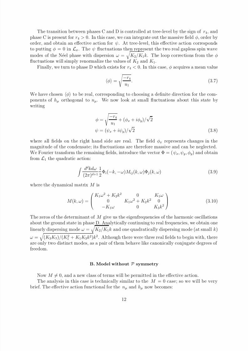
The transition between phases C and D is controlled at tree-level by the sign of r4, andphase C is present for r4 > 0. In this case, we can integrate out the massive field φ, order byorder, and obtain an effective action for ψ. At tree-level, this effective action correspondsto putting φ = 0 in Lσ. The ψ fluctuations then represent the two real gapless spin wave
modes of the Neel phase with dispersion ω = K 2/K 1k. The loop corrections from the φ
fluctuations will simply renormalize the values of K 2 and K 1.Finally, we turn to phase D which exists for r4 < 0. In this case, φ acquires a mean value
φ =
−r4u1
. (3.7)
We have chosen φ to be real, corresponding to choosing a definite direction for the com-ponents of hµ orthogonal to nµ. We now look at small fluctuations about this state bywriting
φ = −r4
u1
+ (φx + iφy)/√
2
ψ = (ψx + iψy)/√
2 (3.8)
where all fields on the right hand side are real. The field φx represents changes in themagnitude of the condensate; its fluctuations are therefore massive and can be neglected.We Fourier transform the remaining fields, introduce the vector Φ = (ψx, ψy, φy) and obtainfrom L1 the quadratic action:
ddkdω
(2π)d+1
1
2Φi(−k, −ω)M ij(k, ω)Φ j(k, ω) (3.9)
where the dynamical matrix M is
M (k, ω) =
K 1ω2 + K 2k2 0 K 1ω
0 K 1ω2 + K 2k2 0−K 1ω 0 K 3k2
(3.10)
The zeros of the determinant of M give us the eigenfrequencies of the harmonic oscillationsabout the ground state in phase D. Analytically continuing to real frequencies, we obtain one
linearly dispersing mode ω =
K 2/K 1k and one quadratically dispersing mode (at small k)
ω =
(K 3K 2)/(K 21 + K 1K 3k2)k2. Although there were three real fields to begin with, thereare only two distinct modes, as a pair of them behave like canonically conjugate degrees of freedom.
B. Model without P symmetry
Now M = 0, and a new class of terms will be permitted in the effective action.The analysis in this case is technically similar to the M = 0 case; so we will be very
brief. The effective action functional for the nµ and hµ now becomes:
12

8/3/2019 Subir Sachdev and T. Senthil- Zero temperature phase transitions in quantum Heisenberg ferromagnets
http://slidepdf.com/reader/full/subir-sachdev-and-t-senthil-zero-temperature-phase-transitions-in-quantum 13/45
Z =
DnµDhµ exp
−
ddx β
0dτ (L1 + L2)
L1 =
K 1
2
∂nµ
∂τ −iµνλ(hν + H ν )nλ
2
+K 2
2
(
nµ)2 +
K 3
2
(
hµ)2
+ K 4(nµ)(hµ) +r12
h2µ +
u1
8(h2
µ)2
L2 =r22
n2µ + r3hµnµ +
u2
8(n2
µ)2 +v12
(n2µ)(h2
ν ) +v22
(nµhµ)2 (3.11)
Note the presence of the additional couplings K 4 and r3; these couplings were forbiddenearlier by the P symmetry.
We can again look for static, spatially uniform, saddle points of L. As before, thisgives three different types of solutions, corresponding to the phases A, C, and D but nonecorresponding to the B phases. The low-lying excitation spectrum can again be found bydefining a hybrid sigma model by imposing the constraints
nµnµ = 1 ; nµhµ = c (3.12)
where c is some constant. Clearly the only difference from the previous section is the non-zero (but constant) value of nµhµ. This is necessary because though the onset of the cantedphase D is still signaled by the appearance of an expectation value of hµ in a directionorthogonal to the mean direction of nµ, the component of hµ parallel to nµ is non-zero inboth the C (Neel) and D phases when M = 0 .
We proceed as before and move well away from phase A, assume that nµ has a welldeveloped expectation value along the z direction, and replace the earlier parametrization(3.5) by the following:
n =
ψ + ψ∗
√2
,ψ − ψ∗
√2i
, (1 − 2|ψ|2)1/2
h = cn +
φ + φ∗√
2,
φ − φ∗√2i
, − ψ∗φ + φ∗ψ
(1 − 2|ψ|2)1/2
. (3.13)
The new feature is the first term in the second equation. From now on the analysis is similarto that in the previous section, so we merely state the results. At the Gaussian level, therenow is a new term in the lagrangian Lσ1 equal to K 5(ψ∗φ + ψφ∗). Both the Neel
and canted phases continue to have the same excitation spectrum as at M = 0, but theconstants of proportionality in the low k dispersion relations are different from their M = 0values, as are the actual eigenvectors corresponding to the normal modes.
IV. QUANTUM PHASE TRANSITIONS
In this section we consider the critical behavior of some of the continuous quantumtransitions among the phases in Fig 1. The transition between the paramagnet A and the
13
8/3/2019 Subir Sachdev and T. Senthil- Zero temperature phase transitions in quantum Heisenberg ferromagnets
http://slidepdf.com/reader/full/subir-sachdev-and-t-senthil-zero-temperature-phase-transitions-in-quantum 14/45
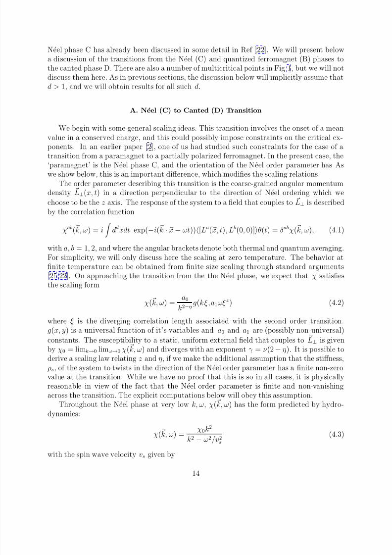
Neel phase C has already been discussed in some detail in Ref [22]. We will present belowa discussion of the transitions from the Neel (C) and quantized ferromagnet (B) phases tothe canted phase D. There are also a number of multicritical points in Fig 1, but we will notdiscuss them here. As in previous sections, the discussion below will implicitly assume thatd > 1, and we will obtain results for all such d.
A. Neel (C) to Canted (D) Transition
We begin with some general scaling ideas. This transition involves the onset of a meanvalue in a conserved charge, and this could possibly impose constraints on the critical ex-ponents. In an earlier paper [2], one of us had studied such constraints for the case of atransition from a paramagnet to a partially polarized ferromagnet. In the present case, the‘paramagnet’ is the Neel phase C, and the orientation of the Neel order parameter has Aswe show below, this is an important difference, which modifies the scaling relations.
The order parameter describing this transition is the coarse-grained angular momentum
density L⊥(x, t) in a direction perpendicular to the direction of Neel ordering which wechoose to be the z axis. The response of the system to a field that couples to L⊥ is describedby the correlation function
χab( k, ω) = i
ddxdt exp(−i( k · x − ωt))[La(x, t), Lb(0, 0)]θ(t) = δabχ( k, ω), (4.1)
with a, b = 1, 2, and where the angular brackets denote both thermal and quantum averaging.For simplicity, we will only discuss here the scaling at zero temperature. The behavior atfinite temperature can be obtained from finite size scaling through standard arguments[25,22]. On approaching the transition from the the Neel phase, we expect that χ satisfiesthe scaling form
χ( k, ω) =a0
k2−ηg(kξ,a1ωξz) (4.2)
where ξ is the diverging correlation length associated with the second order transition.g(x, y) is a universal function of it’s variables and a0 and a1 are (possibly non-universal)
constants. The susceptibility to a static, uniform external field that couples to L⊥ is givenby χ0 = limk→0 limω→0 χ( k, ω) and diverges with an exponent γ = ν (2 − η). It is possible toderive a scaling law relating z and η, if we make the additional assumption that the stiffness,ρs, of the system to twists in the direction of the Neel order parameter has a finite non-zerovalue at the transition. While we have no proof that this is so in all cases, it is physically
reasonable in view of the fact that the Neel order parameter is finite and non-vanishingacross the transition. The explicit computations below will obey this assumption.Throughout the Neel phase at very low k, ω, χ( k, ω) has the form predicted by hydro-
dynamics:
χ( k, ω) =χ0k2
k2 − ω2/v2s(4.3)
with the spin wave velocity vs given by
14
8/3/2019 Subir Sachdev and T. Senthil- Zero temperature phase transitions in quantum Heisenberg ferromagnets
http://slidepdf.com/reader/full/subir-sachdev-and-t-senthil-zero-temperature-phase-transitions-in-quantum 15/45
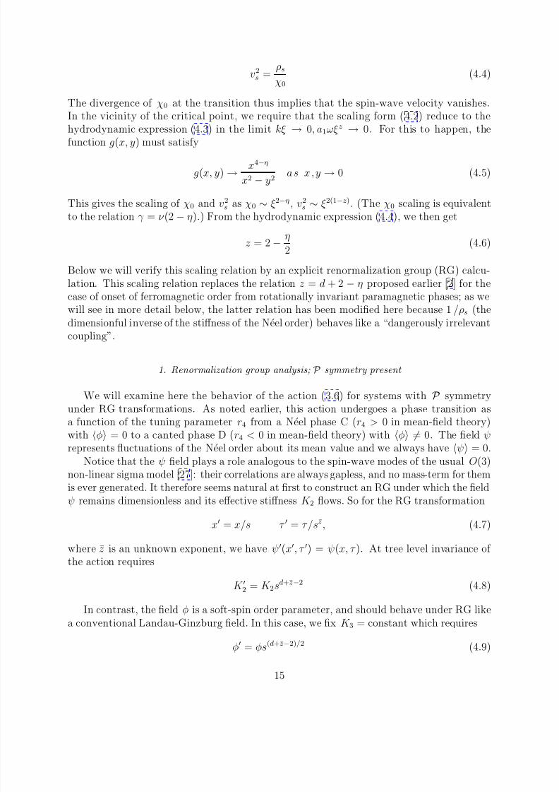
v2s =
ρs
χ0(4.4)
The divergence of χ0 at the transition thus implies that the spin-wave velocity vanishes.In the vicinity of the critical point, we require that the scaling form (4.2) reduce to thehydrodynamic expression (4.3) in the limit kξ
→0, a1ωξz
→0. For this to happen, the
function g(x, y) must satisfy
g(x, y) → x4−η
x2 − y2a s x,y → 0 (4.5)
This gives the scaling of χ0 and v2s as χ0 ∼ ξ2−η , v2
s ∼ ξ2(1−z). (The χ0 scaling is equivalentto the relation γ = ν (2 − η).) From the hydrodynamic expression (4.4), we then get
z = 2 − η
2(4.6)
Below we will verify this scaling relation by an explicit renormalization group (RG) calcu-lation. This scaling relation replaces the relation z = d + 2 − η proposed earlier [2] for thecase of onset of ferromagnetic order from rotationally invariant paramagnetic phases; as wewill see in more detail below, the latter relation has been modified here because 1/ρs (thedimensionful inverse of the stiffness of the Neel order) behaves like a “dangerously irrelevantcoupling”.
1. Renormalization group analysis; P symmetry present
We will examine here the behavior of the action (3.6) for systems with P symmetryunder RG transformations. As noted earlier, this action undergoes a phase transition asa function of the tuning parameter r4 from a Neel phase C (r4 > 0 in mean-field theory)with φ = 0 to a canted phase D (r4 < 0 in mean-field theory) with φ = 0. The field ψrepresents fluctuations of the Neel order about its mean value and we always have ψ = 0.
Notice that the ψ field plays a role analogous to the spin-wave modes of the usual O(3)non-linear sigma model [27]: their correlations are always gapless, and no mass-term for themis ever generated. It therefore seems natural at first to construct an RG under which the fieldψ remains dimensionless and its effective stiffness K 2 flows. So for the RG transformation
x = x/s τ = τ /sz, (4.7)
where z is an unknown exponent, we have ψ(x, τ ) = ψ(x, τ ). At tree level invariance of the action requires
K 2 = K 2sd+z−2 (4.8)
In contrast, the field φ is a soft-spin order parameter, and should behave under RG likea conventional Landau-Ginzburg field. In this case, we fix K 3 = constant which requires
φ = φs(d+z−2)/2 (4.9)
15
8/3/2019 Subir Sachdev and T. Senthil- Zero temperature phase transitions in quantum Heisenberg ferromagnets
http://slidepdf.com/reader/full/subir-sachdev-and-t-senthil-zero-temperature-phase-transitions-in-quantum 16/45
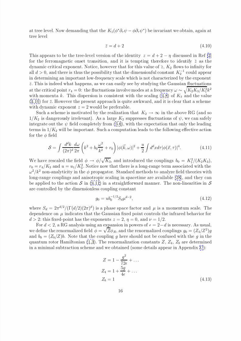
at tree level. Now demanding that the K 1(φ∗∂ τ ψ − φ∂ τ ψ∗) be invariant we obtain, again at
tree level
z = d + 2 (4.10)
This appears to be the tree-level version of the identity z = d + 2
−η discussed in Ref [2]
for the ferromagnetic onset transition, and it is tempting therefore to identify z as thedynamic critical exponent. Notice, however that for this value of z, K 2 flows to infinity forall d > 0, and there is thus the possibility that the dimensionful constant K −12 could appearin determining an important low-frequency scale which is not characterized by the exponentz. This is indeed what happens, as we can easily see by studying the Gaussian fluctuations
at the critical point r4 = 0: the fluctuations involve modes at a frequency ω ∼
K 2K 3/K 21k2
with momenta k. This dispersion is consistent with the scaling (4.8) of K 2 and the value(4.10) for z. However the present approach is quite awkward, and it is clear that a schemewith dynamic exponent z = 2 would be preferable.
Such a scheme is motivated by the realization that K 2 → ∞ in the above RG (and so
1/K 2 is dangerously irrelevant). As a large K 2 suppresses fluctuations of ψ, we can safelyintegrate out the ψ field completely from (3.6), with the expectation that only the leadingterms in 1/K 2 will be important. Such a computation leads to the following effective actionfor the φ field
S =
ddk
(2π)d
dω
2π
k2 + b0
ω2
k2+ r0
|φ( k, ω)|2 +
u
2
ddxdτ |φ(x, τ )|4. (4.11)
We have rescaled the field φ → φ/√
K 3, and introduced the couplings b0 = K 21/(K 2K 3),r0 = r4/K 3 and u = u1/K 23 . Notice now that there is a long-range term associated with theω2/k2 non-analyticity in the φ propagator. Standard methods to analyze field theories with
long-range couplings and anisotropic scaling in spacetime are available [28], and they canbe applied to the action S in (4.11) in a straightforward manner. The non-linearities in S are controlled by the dimensionless coupling constant
g0 = ub−1/20 S dµd−2, (4.12)
where S d = 2πd/2/(Γ(d/2)(2π)d) is a phase space factor and µ is a momentum scale. Thedependence on µ indicates that the Gaussian fixed point controls the infrared behavior ford > 2: this fixed-point has the exponents z = 2, η = 0, and ν = 1/2.
For d < 2, a RG analysis using an expansion in powers of = 2−d is necessary. As usual,we define the renormalized field φ =
√ZφR, and the renormalized couplings g0 = (Z 4/Z 2)g
and b0
= (Z b/Z )b. Note that the coupling g here should not be confused with the g in the
quantum rotor Hamiltonian (1.3). The renormalization constants Z , Z 4, Z b are determinedin a minimal subtraction scheme and we obtained (some details appear in Appendix C):
Z = 1 − g2
72+ . . .
Z 4 = 1 +5g
4+ . . .
Z b = 1 (4.13)
16
8/3/2019 Subir Sachdev and T. Senthil- Zero temperature phase transitions in quantum Heisenberg ferromagnets
http://slidepdf.com/reader/full/subir-sachdev-and-t-senthil-zero-temperature-phase-transitions-in-quantum 17/45
8/3/2019 Subir Sachdev and T. Senthil- Zero temperature phase transitions in quantum Heisenberg ferromagnets
http://slidepdf.com/reader/full/subir-sachdev-and-t-senthil-zero-temperature-phase-transitions-in-quantum 18/45
We define the renormalization of λ by λ0b1/20 = (Z λ/Z )λb1/2. The new values of the
renormalization constants can now be computed to be (Appendix C):
Z = 1 − g2
2
λ2 + 9
(λ2 + 4)(2λ2 + 9)2+ . . .
Z 4 = 1 + g2
λ2 + 20(λ2 + 4)3/2
+ . . .
Z b = 1
Z 2 = 1 +4g
1
(λ2 + 4)3/2+ . . .
Z λ = 1 − g2
2
1
(λ2 + 4)(2λ2 + 9)+ . . . (4.19)
These results require an expansion in powers of g, but the dependence on λ is exact at eachorder. The β functions of g and λ can now be determined
β g = µ∂
∂µg
B
= −g +g2
2
λ2 + 20
(λ2 + 4)3/2
β λ = µ∂
∂µλ
B
= −g2
2
λ(5λ2 + 27)
(λ2 + 4)(2λ2 + 9)2(4.20)
One of the fixed points of (4.20) is the model with P symmetry of Section I V A 1:
λ∗ = 0, g∗ = 4/5. (4.21)
However, this fixed point is unstable in the infrared; the stable fixed point is instead
λ∗ = ∞, (g/λ)∗ = 2; (4.22)
for λ → ∞, the loop corrections become functions of g/λ, which is therefore the appropriatemeasure of the strength of the non-linearities. Near this stable fixed point, the frequencydependence of the propagator is dominated by the iω term and the ω2/k2 term can beneglected. The exponents at this fixed point can be determined as in (4.15) and (4.17) from(4.19) and we find the same exponents as those of the d > 2 Gaussian fixed point:
z = 2 η = 0 ν = 1/2 (4.23)
Although these exponents are the same for d > 2 and for d < 2, it is important to notethat the d < 2 theory is not Gaussian—there is a finite fixed point interaction (g/λ)∗ = 2which will make the scaling functions and finite temperature properties different from thoseof the Gaussian theory. The structure of this non-Gaussian fixed point has been exploredearlier [25,29] in in a different context and more details are provided in Appendix D). Alsonote that the flow of λ to this fixed point is slow, and will lead to logarithmic corrections toscaling.
18
8/3/2019 Subir Sachdev and T. Senthil- Zero temperature phase transitions in quantum Heisenberg ferromagnets
http://slidepdf.com/reader/full/subir-sachdev-and-t-senthil-zero-temperature-phase-transitions-in-quantum 19/45
B. Quantized Ferromagnet (B) to Canted (D) Transition
The ferromagnetic order parameter Lµ is non-zero in both the B and D phase, while
the component of nµ orthogonal to Lµ plays the role of the order parameter. The roles of
nµ and Lµ are therefore reversed from the considerations in Sections III and IV A, and the
analysis here will, in some sense, be dual to the earlier analyses. In the following we willassume that M = 0 and that P is not a good symmetry; the special properties of the M = 0case will be noted as asides.
To begin, we need a rotationally-invariant field theory which describes the dynamics inone of the quantized B phases and across its phase boundary to the D phase. Let us work inthe B0 phase i.e. the phase in which the quantized moment is 0 = 0 per rotor. If we nowproceed with a derivation of the path integral as in Section III, we find that the single sitefunctional integral (3.1) has to be evaluated in a regime in which (3.2) has a minimum at = 0: this is quite difficult to do. We circumvent this difficulty by the following stratagem.We consider a somewhat different model, which nevertheless has a quantized ferromagneticphase (with a moment 0 per site) and a canted phase separated by a second order transition;this model has an enlarged Hilbert space, but the additional states have a finite energy, andwe therefore expect that its transition is in the same universality class as in the originalrotor model. The new model is an ordinary Heisenberg ferromagnet coupled to a quantumrotor model through short-ranged interactions. The Hamiltonian H new = H Heis +H rot +H int
where
H Heis = −∆i,j
S iµS jµ
H rot = g
i
L2iµ − J
i,j
niµn jµ
H int = −(i,j
K i− j S iµLiµ +i,j
M i− j S iµniµ) (4.24)
Here S iµ is an ordinary Heisenberg spin operator acting on a spin 0 representation, and it
commutes with the nµ and Lµ. The K i− j and M i− j are some short-ranged interactions and∆ is a positive constant. (There is an overlap in the symbols for the couplings above withthose used before; this is simply to prevent a proliferation of symbols, and it is understoodthat there is no relationship between the values in the two cases.) The total conservedangular momentum is
i Liµ + S iµ. The Hilbert space on each site consists of the spin 0
states of the Heisenberg spin and the = 0, 1, 2, 3, . . . states of each rotor. Ignoring inter-sitecouplings, the lowest energy states on each site are a multiplet of angular momentum 0,
similar to the B0 phase of the original model.It is now easy to see that H new exhibits a quantized ferromagnetic phase (with a moment
0 per site) and a canted phase for appropriate choices of parameters. First imagine thatall the K i− j ’s and M i− j ’s are zero and that g J . Then naive perturbation theory in J/gtells us that the ground state is a quantized ferromagnet with total angular momentum 0per site. Now imagine introducing non-zero values of the K and M couplings. The rotorvariables then see an effective “magnetic field” that couples to the Liµ, and an effective fieldthat couples to the niµ. The latter has the effect of introducing an expectation value for the
19
8/3/2019 Subir Sachdev and T. Senthil- Zero temperature phase transitions in quantum Heisenberg ferromagnets
http://slidepdf.com/reader/full/subir-sachdev-and-t-senthil-zero-temperature-phase-transitions-in-quantum 20/45
component of nµ parallel to S µ. The “magnetic field” does not introduce an expectationvalue of Lµ if it is weak. As the strength of the “magnetic field” is increased by varying theK i− j ’s, it induces a transition into a phase with a non-zero, non-integer expectation value of
Lµ, and a non-zero expectation value for the component of nµ perpendicular to S µ. Thisis the transition to the canted phase.
The derivation of the path integral of this model is easy; because the Hilbert spacehas now been expanded, we have also have to introduce coherent states of spin 0 at eachtime slice in the Trotter product. The final functional integral will be expressed in termsof the field nµ of the quantum rotor, and a unit vector field sµ (s2µ = 1) representing the
orientation of the spin S µ. Finally, as in Section III, we also impose the constraint nµsµ = cto project out fluctuations which have a local energy cost (this cost is due to the effectivefield, noted above, that acts between the sµ and nµ). Our final form of the modified sigmamodel appropriate for the transition from a quantized ferromagnet B0 to the canted phaseD is
Z = DnµDsµδ
s2
µ − 1
δ (nµsµ − c)exp−
dd
x β
0 dτ L
L = iM 0Aµ(s)∂sµ
∂τ − M 0H µsµ +
K 12
∂nµ
∂τ + iµνλ(ρsν − H ν )nλ
2
+K 22
(nµ)2 +K 32
(sµ)2 + K 4(nµ)(sµ) +r12
n2µ +
u1
8(n2
µ)2 (4.25)
Again there is an overlap in the symbols for the couplings above with those used in Secs IIIand IV B, and it is understood that there is no relationship between the values in the twocases. There is no length constraint on the components of nµ orthogonal to sµ, which actas a soft-spin order parameter for the transition from phase B to phase D. The ρsν term isthe effective internal “magnetic field” (noted above) that the Heisenberg spins impose onthe nµ, with ρ a coupling constant that measures its strength. Note also that
K 4 = c = 0 if P is a symmetry. (4.26)
The coupling M 0 = l0a−d, where ad is the volume per rotor, and, as before, H µ is the externalmagnetic field. The first term in L is the Berry phase associated with quantum fluctuationsof the ferromagnetic moment: Aµ(s) is the vector potential of a unit Dirac monopole at theorigin of s space, and is defined up to gauge transformations by µνλ∂Aλ/∂sν = sµ.
The onset of phase D is signalled by a mean value in nµ orthogonal to the averagedirection of sµ. Using a reasoning similar to that above (3.5), we parametrize the fields of the modified sigma model as
s =
φ + φ∗
2(2 − |φ|2)1/2,
φ − φ∗
2i(2 − |φ|2)1/2, 1 − |φ|2
n = cs +
ψ + ψ∗
√2
,ψ − ψ∗
√2i
, −(ψ∗φ + φ∗ψ)(2 − |φ|2)1/2√2(1 − |φ|2)
. (4.27)
20
8/3/2019 Subir Sachdev and T. Senthil- Zero temperature phase transitions in quantum Heisenberg ferromagnets
http://slidepdf.com/reader/full/subir-sachdev-and-t-senthil-zero-temperature-phase-transitions-in-quantum 21/45
We have chosen a non-standard parametrization of the unit vector field sµ in terms of a complex scalar φ: this choice is a functional integral version of the Holstein-Primakoff decomposition of spin operators, and ensures that the Berry phase term iM 0Aµ(s)(∂sµ/∂τ )is exactly equal to M 0φ∗(∂φ/∂τ ). The parametrization of nµ then follows as in (3.5) andensures that nµsµ = c. The two complex fields ψ, φ, correspond to the 4 degrees of freedom
of the hybrid sigma model. The field φ represents oscillations of the s about its mean value:by definition, we will have φ = 0 in both the B and D phases. The field ψ measuresthe amplitude of nµ orthogonal to the instantaneous value of sµ: we have ψ = 0 in thequantized ferromagnet B, while ψ = 0 in the canted phase D. We now insert ( 4.27) into(4.25) and obtain
Z σ =
DψDψ∗DφDφ∗
1 − |φ|2 exp
−
ddx β
0dτ (Lσ + · · ·)
Lσ = M 0φ∗∂φ
∂τ + K 5ψ∗∂ψ
∂τ + K 6
ψ∗∂φ
∂τ + φ∗
∂ψ
∂τ
+ H z−M 0 + M 0|φ|
2
+ K 5|ψ|2
+ K 6(ψ
∗
φ + ψφ
∗
)
+ K 2|ψ|2 + K 7|φ|2 + K 8(ψ∗φ + ψφ∗)
+ r2
|ψ|2 +
1
2(ψ∗φ + ψφ∗)2
+
u1
2|ψ|4 (4.28)
where K 5 = 2ρK 1, K 6 = cρK 1, K 7 = K 3 + 2cK 4 + c2K 2, K 8 = K 4 + cK 2, r2 = r1 −K 1ρ2 + u1c2/2. Stability of the action requires that K 2 > 0, K 7 > 0, and K 2K 7 > K 28 ; theseconditions will be implicitly assumed below, and are the analog of the requirement in themean-field theory of Section II that M not be too large. Without loss of generality, we canassume that M 0 > 0; however the signs of K 5 and M 0K 5 − K 26 can be arbitrary, and thesewill play an important role in our analysis below. Systems with M = 0, and the symmetry
P , will have K 6 = K 8 = 0. We have explicitly displayed only terms up to quartic order inthe fields. Anticipating the RG analysis below, we have also dropped irrelevant terms withadditional time derivatives. The field H µ = (0, 0, H z) has been assumed to point along thez direction.
Notice that the coupling to H z could have been deduced by the gauge invariance prin-ciple [2] which demands the replacement ∂/∂τ → ∂/∂τ + H z (∂/∂τ → ∂/∂τ − H z) whenacting on the φ, ψ (φ∗, ψ∗) fields. The magnetization density, M is given by
M = − ∂ F ∂H z
, (4.29)
where
F is the free energy density. The gauge invariance of the action ensures that at T = 0,
this magnetization density is exactly M 0, as long as ψ = 0 i.e. we are in phase B.We can easily do a small fluctuation, normal mode, analysis in both phases of ( 4.28). In
the quantized ferromagnetic phase B (r2 > 0) we have the usual ferromagnetic spin waveswith ω = K 7k2/M 0 at small k and also a massive mode with ω ∼ r2/(K 5 − K 26/M 0) (wehave assumed here and in the remainder of the paragraph that H z = 0). The massive modebecomes gapless at r2 = 0, signaling the onset of the canted phase D. In this canted phase,
we have ψ =
−r2/u1. Analysis of fluctuations about this mean value for ψ gives twoeigenfrequencies which vanish as k → 0; the first has a linear dispersion
21
8/3/2019 Subir Sachdev and T. Senthil- Zero temperature phase transitions in quantum Heisenberg ferromagnets
http://slidepdf.com/reader/full/subir-sachdev-and-t-senthil-zero-temperature-phase-transitions-in-quantum 22/45
ω2 =2|r2|W
(M 0K 5 − K 26 )2k2, (4.30)
while the second disperses quadratically
ω
2
=
K 7(K 2K 7
−K 28 )
W k
4
, (4.31)
where W = (M 0√
K 2 − K 6√
K 7)2 + 2K 6M 0(√
K 2K 7 − K 8) > 0. These results for phase Dare in agreement with those obtained earlier using a ‘dual’ approach with the action ( 3.6)in Sections IIIA and IIIB.
It is also useful to compare and contrast the action (3.6) for the transition from C to Dwith the action (4.28) above for the B to D transition. Notice that the roles of the fieldsare exactly reversed–in the former φ was the order parameter for the transition while ψdescribed spectator modes which were required by symmetry to be “massless”; in the latterψ is the order parameter while φ is “massless” spin-wave mode. The two models howeverdiffer significantly in the nature of the time derivative terms in the action. In (4.28) there
are terms linear in time derivatives for both the ψ and φ fields, while there are no suchterms in (3.6) (the time derivative term involving an off-diagonal φ, ψ coupling is presentin both cases, though). As a result the spectator spin-wave φ mode in (4.28) has ω ∼ k2,while the spectator spin-wave ψ mode in (3.6) has ω ∼ k. These differences have significantconsequences for the RG analysis of (4.28), which will be discussed now.
1. Renormalization group analysis
The logic of the analysis is very similar to the ‘dual’ analysis in Sections I V A 1 and I V A 2.We expect the stiffness of the spectator φ modes flows to infinity, and hence it is valid to
simply integrate out the φ fluctuations. This gives us the following effective action for the ψfield (which, recall, measures the value of nµ in the direction orthogonal to the ferromagneticmoment):
S =
ddk
(2π)d
dω
2π
−iK 5ω + K 2k2 − (−iK 6ω + K 8k2)2
−iM 0ω + K 7k2+ r2
|ψ( k, ω)|2
+u1
2
ddxdτ |ψ(x, τ )|4. (4.32)
We have written the action for H z = 0, and the H z dependence can be deduced from themapping −iω → −iω + H z. Simple power-counting arguments do not permit any further
simplifications to be made to this action. Despite the apparent formidable complexity of itsform, the RG properties of (4.32) are quite simple, as we shall now describe.We will consider the cases with and without P symmetry separately.
a. P symmetry present
Now we have K 6 = K 8 = 0. The non-analytic terms in the propagator of (4.32) disappear,and the remaining terms are identical to those in the action of a dilute Bose gas with a
22
8/3/2019 Subir Sachdev and T. Senthil- Zero temperature phase transitions in quantum Heisenberg ferromagnets
http://slidepdf.com/reader/full/subir-sachdev-and-t-senthil-zero-temperature-phase-transitions-in-quantum 23/45
repulsive interaction u1. The order parameter, ψ, and the spectator modes, φ, are essentiallyindependent, with all couplings between them contributing only “irrelevant” corrections tothe leading critical behavior.
The critical theory of the quantum transition in the dilute Bose gas has been studied ear-lier [25,29] (see Appendix D), and also appeared as the fixed point theory in Section I V A 2.
A measure of the strength of the loop corrections is the dimensionless coupling constant g0(the analog here of Eqn (4.12))
g0 = u1K −12 |K 5|−1S dµd−2 (4.33)
(where, as before, µ is a renormalization momentum scale, S d is a phase space factor, andthe symbol g is not to be confused with the coupling g in (1.3)), which determines thescattering amplitude of two pre-existing excitations. This amplitude undergoes a one-looprenormalization due to diagrams associated with repeated scattering of the two excitations,a process which leads to the β function
β g = −g + g
2
2 (4.34)
where = 2−d and we have used the minimal subtraction method to define the renormalizedg (this β function is in fact exact to all orders in g—see Appendix D). The infrared stablefixed point is g∗ = 0 for d > 2, and g∗ = 2 for d < 2. The exponents take the same valuesas in Section I V A 2
z = 2 η = 0 ν = 1/2. (4.35)
for all values of d. It is important to note, however, that the present subsection and Sec-tion I V A 2 have very different interpretations of the order parameter. In Section I V A 2 the
exponent η is associated with the field φ which is proportional to the ferromagnetic moment.Here the η refers to the the field ψ, and the ferromagnetic order parameter scales as |ψ|2 aswe discuss below.
The magnetization density order parameter M(x, τ ), is defined by generalizing (4.29)a space-time dependent external magnetic field H z(x, τ ). In the quantized ferromagneticphase B, clearly M = M 0. Therefore, the deviation M 0 − M can serve as another orderparameter for the B to D transition. Indeed, this order parameter scales as |ψ|2, and we candefine an associated “anomalous” dimension ηM. A simple calculation shows that ηM = d,and so the identity [2]
z = d + 2 − ηM (4.36)is always satisfied. As in Ref [29], we can also compute the behavior of the mean value of this conserved order parameter in the canted phase D. For d < 2, this behavior is universaland is given by
M = M 0 − sgn(K 5)θ(−r2)Cd
|r2|K 2
d/2
, (4.37)
23
8/3/2019 Subir Sachdev and T. Senthil- Zero temperature phase transitions in quantum Heisenberg ferromagnets
http://slidepdf.com/reader/full/subir-sachdev-and-t-senthil-zero-temperature-phase-transitions-in-quantum 24/45
where Cd is a universal number; we compute Cd in an expansion in in Appendix D. Note thatthe magnetization density can increase or decrease into the ferromagnetic phase, dependingupon the sign of K 5; this behavior is consistent with that of the mean field theory inSection II. Note also that (4.37) is independent of the magnitude of K 5. The magnitudeof K 5 however does determine the width of the critical region within which (4.37) is valid.
For |K 5| smaller than √r2, it becomes necessary to include the leading irrelevant frequencydependence in the propagator of (4.32) - a ω2|ψ( k, ω)|2 term. The point K 5 = 0 is a specialmulticritical point at which this new term is important at all values of r2; this multicriticalpoint has z = 1 [25], and has M continue to equal M 0 (to leading order) in phase D.
b. P symmetry absent
The theory without P symmetry is somewhat more involved, and it is convenient to workwith a more compact notation. We rescale ψ( k, ω) → (M 0/
√W K 7)ψ( k, ω), ω → ωK 7, and
manipulate (4.32) into the form
S = ddk
(2π)d
dω
2π
−iλ0M 0ω + k2 − b0
k4
−iM 0ω + k2+ r0
|ψ( k, ω)|2
+u
2
ddxdτ |ψ(x, τ )|4, (4.38)
where r0 = M 20 r2/W , u = u1K 7M 40 /W 2, λ0 = K 7(M 0K 5 − K 26 )/W , and b0 = (K 6K 7 −K 8M 0)2/W K 7. Notice that we have introduced two dimensionless couplings, λ0 and b0,while M 0 has the dimensions of time/(length)2. The stability conditions discussed below(4.28) imply that 0 ≤ b0 < 1.
We now discuss the renormalization of the theory (4.38) as a perturbation theory in the
dimensionless coupling constant
g0 = uS dµd−2/(M 0|λ0|), (4.39)
which is the analog of (4.33). A key property of this perturbation theory, similar to thatnoted in Section I V A 1, is that no terms sensitive to the ratio ω/k2, as ω → 0, k → 0, areever generated. As a result the term multiplying b0 in (4.38) does not undergo any directrenormalization. With this in mind, we define the renormalized field by ψ =
√ZψR, and the
renormalized couplings by λ0 = (Z λ/Z )λ, b0 = (1/Z )b, r0 = (Z 2/Z )r and g0 = (Z 4/Z 2)g. Itremains to compute the renormalization constants Z , Z λ, Z 2, and Z 4.
In the perturbation theory in g, the sign of λ (which is also the sign of M 0K 5
−K 26) plays
a crucial role. The physical interpretation of this sign is the following: when λ > 0, thespin wave quanta, φ, and the order parameter quanta, ψ, carry the same magnetic moment;however for λ < 0 they carry opposite magnetic moments. This was already clear in theK 6 = 0 result (4.37), where the condensation of ψ lead to a decrease or increase in the meanmagnetization density depending upon the sign of K 5. For λ < 0, it is then possible to havea low-lying excitation of a ψ and a φ quantum, which has the same spin as the ground state.For the system without P symmetry, such an excitation will mix with the ground state, andleads to some interesting structure in the renormalization group. In the actual computation,
24
8/3/2019 Subir Sachdev and T. Senthil- Zero temperature phase transitions in quantum Heisenberg ferromagnets
http://slidepdf.com/reader/full/subir-sachdev-and-t-senthil-zero-temperature-phase-transitions-in-quantum 25/45
the sign of λ determines the location of the poles of the propagator of (4.38) in the complexfrequency plane. A simple calculation shows that the propagator has two poles, and bothpoles are in the same half-plane for λ > 0, while for λ < 0 the poles lie on opposite sides of the real frequency axis. We will consider these two cases separately below:λ > 0
For the case where the poles are in the same half-plane, we can close the contour of frequencyintegrals in the other half-plane, and as a result many Feynman diagrams are exactly zero.In particular, all graphs in the expansion of the self energy vanish. As a result, we have
Z = Z λ = Z 2 = 1 (4.40)
There is still a non-trivial contribution to Z 4 (from the ‘particle-particle’ graph):
Z 4 = 1 +g
2
(λ + 1 − b)
(1 − b)(1 + λ)(4.41)
where, as before = 2−
d. These renormalization constants lead to the β functions
β b = 0
β λ = 0
β g = −g +g2
2
(1 + λ − b)
(1 − b)(1 + λ)(4.42)
The vanishing of β b and β λ is expected to hold to all orders in g; as a result, b and λare dimensionless constants which can modify the scaling properties. The exponents arehowever independent of the values of b and λ, and are identical to those of the system withP symmetry, discussed above in Section I V B 1a. The upper critical dimension is 2, and for
d < 2 the magnetization density obeys an equation similar to (4.37)
M = M 0 − θ(−r0)Cd|r0|d/2. (4.43)
The ‘universal’ number Cd now does depend upon b and λ: the leading term in Cd can becomputed by using the gauge-invariance argument to deduce the modification of ( 4.38) ina field, using (4.29) to determine the expression for M [30], determining the fixed point of β g, and then using the method of Ref [29]—this gives
Cd =S d2
1 +
b
λ
(1 − b)(1 + λ)
1 + λ − b(4.44)
This result should be compared with the first term in (D12), which is the value of Cd for theBose gas. Terms higher order in are also expected to be modified by b and λ, but havenot been computed. The results (4.43), (4.44) are not useful for too small a value of λ: thereasons are the same as those discussed below (4.37) but with λ playing the role of K 5.λ < 0The computations for λ < 0 are considerably more involved and are summarized in Ap-pendix E. From (E5), (E6) and (E8) we can deduce the renormalization constants
25
8/3/2019 Subir Sachdev and T. Senthil- Zero temperature phase transitions in quantum Heisenberg ferromagnets
http://slidepdf.com/reader/full/subir-sachdev-and-t-senthil-zero-temperature-phase-transitions-in-quantum 26/45
Z = 1 − g2
2R1(b, λ)
Z λ = 1 − g2
2λR2(b, λ)
Z 4 = 1 +g
2
R3(b, λ)
Z 2 = 1 +g
R4(b, λ), (4.45)
where R1, R2, R3, R4 are functions of b and λ defined in (E7,E9). These now lead to the β functions
β b = g2bR1(b, λ)
β λ = g2(λR1(b, λ) − R2(b, λ))
β g = −g + g2R3(b, λ)/2. (4.46)
It is not difficult to deduce the consequences of these flows by some numerical analysis aidedby asymptotic analytical computations.
For d ≥ 2 ( < 0) we have b(µ) → b∗, λ(µ) → λ∗, g(µ) → 0 in the infrared (µ → 0).Here 0 < b∗ < 1 and λ∗ < 0, but the values of b∗, λ∗ are otherwise arbitrary and determinedby the initial conditions of the flow; they acquire only a finite renormalization from theirinitial vales. The flow to this final state has a power-law dependence on µ for < 0, whileit behaves likes ∼ 1/ log(1/µ) for = 0. The properties of the final state have only minordifferences from λ > 0 case discussed above, and we will not elaborate on them.
The possible behaviors are somewhat richer for > 0. The flow in the infrared is eitherto a fixed line or a fixed point.(i ) The fixed line is 2/3 < b∗ < 1, λ∗ = 0, g∗ = 2; the flow of g to g∗ is a power-law in µ,
while that of b and λ is logarithmic:
λ(µ) = − (1 − b∗)
22b∗(3b∗ − 2) log(1/µ), b(µ) − b∗ =
(1 − b∗)2
42(3b∗ − 2)2 log(1/µ). (4.47)
(ii ) The fixed point is b∗ = 0, λ∗ = −∞, g∗ = 2; again the flow of g to g∗ is a power-law inµ, while that of b and λ is logarithmic:
λ(µ) ∼ −(log(1/µ))1/3 , b(µ) ∼ (log(1/µ))−1/3. (4.48)
The exponents at both the fixed line and the fixed point take the same values as in ( 4.35).
However the flows above will lead to logarithmic corrections which can be computed bystandard methods. The prefactors of the these corrections, and also some amplitude ratios,will vary continuously with the value of b∗ along the fixed line.
V. ROTORS WITH A NON-ZERO MIMIMUM ANGULAR MOMENTUM
We now consider an extension of the rotor model H in which each rotor has a ‘magneticmonopole’ at the origin of n space. Our motivations for doing this are: (i ) It allows for
26
8/3/2019 Subir Sachdev and T. Senthil- Zero temperature phase transitions in quantum Heisenberg ferromagnets
http://slidepdf.com/reader/full/subir-sachdev-and-t-senthil-zero-temperature-phase-transitions-in-quantum 27/45
quantized ferromagnetic states in which the moment is a half-integer times the number of rotor sites. Such phases will occur in cases in which each rotor corresponds to an odd numberof Heisenberg spins in an underlying spin model. (ii ) In d = 1 (to be discussed in Sec VI)such rotor models will lead, by the construction of Ref [31], to Neel phases described by asigma model with a topological theta term.
Following the method of Wu and Yang [32], we generalize the form (1.2) of Lµ to
Liµ = −µνλniν
∂
∂nλ+ qεiAλ(niµ)
− qεiniµ (5.1)
where q is chosen to have one of the values 1/2, 1, 3/2, 2, 5/2, . . . and Aµ(n) is the vectorpotential of a Dirac monopole at the origin of n space which satisfies µνλ∂Aλ/∂nν = nµ (weconsidered this same function in Sec IV B for different reasons). We will work exclusivelyon bipartite lattices and choose εi = 1 (εi = −1) on the first (second) sublattice: we willcomment below on the reason for this choice. It can now be verified that (5.1) continues tosatisfy the commutation relations (1.1) for all q. However the Hilbert space on each site is
restricted to states |, m satisfying L2µ|q,,m = ( + 1)|q,,m with = q, q + 1, q + 2, . . .and m = −, − + 1, . . . , [32]. Notice that there is a minimum value, q, to the allowedangular momentum.
Another consequence of a non-zero q is that it is no longer possible to have P as asymmetry of a rotor Hamiltonian. There is a part of Lµ in (5.1) which is proportional to
nµ, and this constrains Lµ, nµ to have the same signature under discrete transformations:this rules out P as a symmetry, even in models with M = 0.
Our insertion of the εi in (5.1) is also related to the absence of the P symmetry for q > 0.Because Lµ and nµ have the same signature under all allowed symmetries for q > 0, theirexpectation values turn out to be proportional to each other on a given site, with the sign of the proportionality constant determined by εi (we will see this explicitly below). In a q > 0model with εi = 1 on every site, the spatial average of nµ is proportional to that of Lµand therefore to the net ferromagnetic moment; as a result, such models turn out to haveonly quantized ferromagnetic phases. Staggering of εi is a way of inducing a Neel-like orderparameter with no net moment; then a spatially uniform value of nµ represents a staggered
mean value of the angular momentum Lµ, as expected from a Neel order parameter. Thestaggering of εi was also present in the d = 1 analysis of Ref [31], and was crucial there ingenerating the topological theta term.
We present in Fig 2 the mean field phase diagram of the Hamiltonian H (Eqn (1.3))on a bipartite lattice with M = 0, Lµ given by (5.1), and q = 1/2. Because of absence of the P symmetry, a non-zero M will not make a qualitative difference. Other values of the
q are also expected to have a similar phase diagram. The caption describes the non-zerocomponents of Lµ and nµ in the various phases. The expectation values nµ have exactly
the same form as the Lµ in spin space, but the opposite signature in sublattice space (e.g.
a staggered configuration of Lx implies a uniform configuration of nx and vice versa).The phases in Fig 2 are closely related to those in Fig 1. As before we have the quantized
ferromagnetic phases B (albeit, now with half-integral moments), the Neel phase C, and thecanted phase D. The main difference is in the absence of a quantum paramagnetic phaseA: this is clearly due to the minimum allowed value q = 1/2 in the single rotor angular
27
8/3/2019 Subir Sachdev and T. Senthil- Zero temperature phase transitions in quantum Heisenberg ferromagnets
http://slidepdf.com/reader/full/subir-sachdev-and-t-senthil-zero-temperature-phase-transitions-in-quantum 28/45
momentum.It is now possible to undertake an analysis of the low energy properties of the phases,
and of the critical properties of the phase transitions, much like that carried out in Secs IIIand IV for the q = 0 case: such an analysis shows essentially no differences between q = 0and q > 1, at least for d > 1. The excitations of the phases B, C, and D in Fig 2 are
the same as those of the corresponding phases in Fig 1, as are the universality classes of the continuous phase transitions between C and D, and between B and D. One small, butimportant, point has to be kept in mind in this regard. The q > 0 models are not invariantunder the symmetry P even when M = 0, and so the restrictions that the P symmetryimplies for the q = 0 analysis of Secs III and IV must not be imposed now.
In d = 1, there are significant differences between the q = 0 and q = 1/2 cases, and thesewill be discussed in the next section.
VI. QUANTUM ROTORS IN ONE DIMENSION
The general topology of the mean-field phase diagrams Figs 1 and 2 is expected tohold for all d > 1. As we have seen in Sec IV, for d < 2 fluctuations do modify thecritical properties of the continuous transitions, but these modifications are computable ina systematic expansion in 2 − d. In d = 1, fluctuations modify not only the transitions, butalso the stability of the phases: as a result, we expect significant changes in the topology of the phase diagram itself. Further, we also expect a sensitive dependence to the value of themonopole charge q. In the following, we present a mixture of results, educated surmises andspeculation on the nature of the phases and phase transitions in d = 1 for different valuesof q.
A. q = 0
The expected phase diagram is shown in Fig 3. We discuss some of the important fea-tures in turn:(i ) There is no phase with Neel order (the analog of phase C for d > 1); it has been pre-empted mostly by the quantum paramagnet A. Fluctuations in the incipient Neel phasewould be described by a O(3) non-linear sigma model in 1 + 1 dimensions (without a topo-logical term), which is known not to have a phase with long-range order.(ii ) The quantized ferromagnetic phases, B, are stable even in d = 1. They have the usualω ∼ k2 spectrum of spin-wave excitations.(iii ) The canted phase D has been replaced by a novel new phase E - the partially polarized
ferromagnet. The phase E has true long-range order in the ferromagnetic order parameterLz; however the value of Lz is not quantized and varies continuously. The canted phaseD, in d > 1, also had long-range order in n in the x−y plane; in contrast, in phase E (d = 1)this long- range order has been replaced by a quasi-long-range XY order i.e. correlations of n decay algebraically in the x − y plane. The only true broken symmetry is that associatedwith Lz, and the system is invariant with respect to rotations about the z axis (comparewith phase D in which the O(3) symmetry was completely broken and there was no invariantaxis). Note that though there is no LRO in the x − y plane in phase E, the Goldstone mode
28
8/3/2019 Subir Sachdev and T. Senthil- Zero temperature phase transitions in quantum Heisenberg ferromagnets
http://slidepdf.com/reader/full/subir-sachdev-and-t-senthil-zero-temperature-phase-transitions-in-quantum 29/45
of phase D, associated with it’s x−y LRO survives i.e. phase E has not only a gapless modeω ∼ k2 due to ferromagnetic long-range order, but also a gapless mode ω ∼ k due to quasiLRO in the n field. All of these results follow from a straightforward analysis of the actions(4.25) and (4.28) in d = 1.(iv ) A few remarks about the universality class of the phase transition between phases B and
E. The theory (4.28) should continue to apply. The expansion in = 2 − d (Section I V B 1)should be valid all the way down to d = 1 [29], although it may not be quantitatively accu-rate. The theory with P symmetry has critical properties identical to a dilute Bose gas, andwas discussed in Ref [29] and solved there by a fermionization trick. The theory without P symmetry, has non-analytic terms in the action, and is probably not amenable to a simplesolution by fermionization.(v ) The phase transition between phase A and phase E is always expected to be first-order.The quantum paramagnetic phase A has no gapless excitations and a vanishing spin sus-ceptibility. It is then difficult to conceive of a mechanism which could lead to a continuouscondensation of the field hµ in an action like (3.3) and (3.6) (or (3.11) for M = 0): integrat-ing out the N µ fluctuations does not yield a negative contribution to the “mass”, r1, of the
hµ field, as the spin susceptibility is zero.
B. Integers q > 0
The phase diagram is shown in Fig 4. All of the phases are identical to those discussedabove for q = 0. The only difference is in the behavior of the first-order line surroundingphase A: it bends down towards the origin of the J -K plane, as the minimum possible valueof the single site angular momentum always forces in quantized ferromagnetic phases for J small enough.
C. Half-integers q > 0
The phase diagram is shown in Fig 5. The topology is now similar to the positive integercase, as are the phases B and E, and the transitions between them. The primary differenceis that the quantum paramagnet A has been replaced by a critical phase F, which has nobroken symmetries and power-law decay of all observables. Fluctuations in phase F aredescribed by the 1 + 1 dimensional O(3) non-linear sigma model with a topological termwith coefficient θ = π: this mapping follows from the analysis of Ref [31].
Finally, we make a few remarks on the transition between the critical phase F andthe partially polarized ferromagnet E. As F has gapless excitations, this transition can be
continuous. A (strongly-coupled) field theory for this transition is given by the action L1
in (3.11), supplemented by the constraints (3.12) and a topological term at θ = π in theunit-vector N µ field. An alternative, Hamiltonian point-of-view on the same transition is thefollowing. It is known [33] that the critical 1 + 1 dimensional O(3) non-linear sigma modelis equivalent to the SU (2) Wess-Zumino-Witten model [34] at level k = 1. The Hamiltonianof this model is given by
H WZW = α( J 2L + J 2R) (6.1)
29
8/3/2019 Subir Sachdev and T. Senthil- Zero temperature phase transitions in quantum Heisenberg ferromagnets
http://slidepdf.com/reader/full/subir-sachdev-and-t-senthil-zero-temperature-phase-transitions-in-quantum 30/45
where J L,R are the SU (2) currents obeying a Kac-Moody algebra. We now want to inducea ferromagnetic moment into the ground state of this theory. The action (3.11) does this bycoupling in a fluctuating magnetic field hµ. Such a field would couple here to the magneti-
zation J L + J R: integrating out hµ would then induce a coupling −( J L + J R)2 which givesus the Hamiltonian [35]
H F →E = α( J 2L + J 2R) − λ J L · J R. (6.2)
The model H F →E can also be used to describe the onset of ferromagnetism in an itinerantLuttinger liquid. It has in fact been examined earlier by Affleck [36], where he obtained itas an effective model for the spin degrees of freedom in a d = 1 Hubbard model. Affleckexamined the RG flows of λ for small λ and obtained
dλ
d= −λ2 (6.3)
. In the mapping from the repulsive Hubbard model, and also from our rotor model, the
initial sign of λ is positive. From (6.3), Affleck concluded that λ is irrelevant for all positiveλ, and that all such systems flow into the λ = 0 fixed point. We believe this conclusion isincorrect. It is clear from our arguments that for λ large enough, H F →E should undergo aphase transition to ferromagnetic ground state. This suggests that there is a critical valueof λ = λc (with λc > 0 and of order unity) such that only systems with λ < λc flow into theλ = 0 fixed point. Systems with λ > λc are in the ferromagnetic phase E. The nature of the critical point at λ = λc, which controls the transition from phase F to E, is unknown:determining its structure remains an important open problem.
VII. CONCLUSIONS
This paper has introduced and analyzed the simplest model with Heisenberg symmetrywhich exhibits zero temperature phase transitions, and whose phases contain a net averagemagnetic moment. The model contained only bosonic quantum rotor degrees of freedomand offers the simplest realization of a quantum transition with an order parameter whichis also a non-abelian, conserved charge. The analysis focussed primarily on the HamiltonianH in (1.3), although variations were also considered. The results are summarized in thephase diagrams in Figs 1-5.
Some important properties of these phase diagrams deserve reiteration. Notice that ford > 1, there is no phase which is simply a non-quantized ferromagnet, with no other broken
symmetry. Phase D has a non-quantized ferromagnetic moment, but it has an additionallong-range order in the n field in a plane perpendicular to the ferromagnetic moment. Webelieve this is a generic feature of insulating spin systems: ferromagnetic ground states eitherhave an integral or half-integral magnetic moment, or have an additional broken symmetry.Only in d = 1 does a phase like E appear: it has a non-quantized ferromagnetic moment,and is invariant under rotations about the ferromagnetic axis. However, even in d = 1 thereis a remnant of the broken symmetry in the n field perpendicular to the moment: correlatorsof n have a power-law decay in space, and the linearly-dispersing gapless spin-wave mode
30
8/3/2019 Subir Sachdev and T. Senthil- Zero temperature phase transitions in quantum Heisenberg ferromagnets
http://slidepdf.com/reader/full/subir-sachdev-and-t-senthil-zero-temperature-phase-transitions-in-quantum 31/45
is still present (in addition to the usual quadratically dispersing ferromagnetic mode). Itis also interesting to note that metallic, Fermi liquids of course have no trouble formingnon-quantized ferromagnets; this is in keeping with popular wisdom that Fermi liquids are“effectively” one dimensional.
A second interesting property of the phase diagram was pointed out in Section I: contin-
uous zero temperature transitions in which there is an onset in the ferromagnetic momentonly occur from phases which have gapless excitations. Thus there is such an onset fromphase C (which has gapless spin waves) to phase D, but no continuous transition betweenphases A and D.
We also examined the critical properties of the second order phase transitions in themodel. In several cases, the critical theories turned out to be variations on the themeof a simpler quantum phase transition: the onset of density in a Bose gas with repulsiveinteractions as its chemical potential is moved through zero. This quantum transition hadbeen studied earlier [25,29]. Because of its central importance, we obtained some additionalresults on its T = 0 universal properties in Appendix D.
In the remainder of this section, we remark on issues related to those considered in this
paper, but which we have not directly analyzed here.
1. Itinerant ferromagnets
We discuss implications of our results for quantum phase transitions in ferromagneticFermi liquids. As noted in Section I, there are two quantum transitions in this system, andwe will discuss them separately:(i ) Consider first the transition from a fully polarized Fermi liquid to a partially polarizedFermi liquid. This is rather like the transition from phase B to phase D in d > 1, andthe transition from phase B to phase E in d = 1. Let us suppose that all electrons in the
fully polarized state are polarized in the ‘up’ direction. Then an order parameter for thetransition is simply the density of ‘down’ spin electrons. Along the lines of the analysis inthe rotor model, we can derive an effective action for the down spin electrons simply byintegrating out the up electrons. It turns out that the up electrons only mediate irrelevantinteractions between the down electrons: the effective action for the down electrons is simplythat of a dilute gas of free spinless fermions [2,37]. A possible four-point interaction like the|ψ|4 term for the Bose gas is prohibited by Fermi statistics; further a singular term, like thatappearing in the models without P symmetry in Section I V B 1b, appears to be prohibitedhere because the large Fermi momentum of the up electrons inhibits strong mixing withdown electrons via emission of ferromagnetic spin waves. The properties of the free spinless
fermion model are of course trivial, but it is quite useful to re-interpret them in the languageof a quantum phase transition [37]. It is also interesting to note here that the critical theoryof free spinless fermions in d = 1 is identical to that of dilute interacting bosons for theB to E transition in d = 1 [29]. This is in keeping with our assertion that in d = 1, thetransitions in itinerant fermion systems are in the same universality class as those in certainrotor models.(ii ) Consider now the onset of ferromagnetism in an unpolarized Fermi liquid. A theory forthis transition for d > 1 was proposed by Hertz [4]. This transition is similar to the transition
31
8/3/2019 Subir Sachdev and T. Senthil- Zero temperature phase transitions in quantum Heisenberg ferromagnets
http://slidepdf.com/reader/full/subir-sachdev-and-t-senthil-zero-temperature-phase-transitions-in-quantum 32/45
between phases C and D studied in Section IV A. In the end, our analysis used a methodvery close in spirit to that use by Hertz: simply integrate out all gapless modes not directlyrelated to the order parameter. We have provided here some independent justification forsuch an approach in the rotor model, and our results provide support for the correctness of Hertz’s analysis for d > 1. Precisely in d = 1, we have no theory for the transition between
phases F and E, but we have argued that it should be in the same universality class as that of the onset of ferromagnetism in a Luttinger liquid of itinerant electrons. The critical theoryof this transition is the main remaining open problem in the theory of phase transitions inquantum ferromagnets.
2. Finite temperature
Essentially all the analysis of this paper was at T = 0, and it would be interestingto extend it to finite T . The finite T properties of the quantum paramagnetic phase A,the Neel phase C, and the transition between them, have already been studied in some
detail [21,22]. More recently, a field-theoretic analysis of the finite T properties above aquantized ferromagnetic state B has appeared [16]. It remains, therefore, to study thecanted phase D and its phase transitions at finite T . We have shown in this paper thatthe transition between the B and D phase is similar (although not identical) to that in adilute Bose gas [25,29]—the finite T analysis should therefore be related to that in Ref [29].The finite T properties of the phase D itself should also be quite interesting, especially ind = 2 where the long-range order disappears at any finite T . This is also the case of directrelevance to the quantum Hall effect experiments of Ref [11]. The phase D could be modelede.g. by the action (4.25), supplemented by the additional constraint n2
µ = 1, which can beimposed once we are well away from phase B.
3. Effects of randomness
At T = 0, but in the presence of randomness, one might expect that between the quan-tized ferromagnetic (B) and canted phases (D), there occurs a “canted glass” phase with anon-quantized magnetic moment, short-range mean Neel correlations, but a diverging meanNeel susceptibility; this can be seen by arguments analogous to those in Ref [25]. Further,general arguments [38] imply that for arbitrarily weak randomness in d ≤ 2 and for suffi-ciently strong randomness in d > 2, all the first order lines in our phase diagram are replacedby second-order transitions (implying, for instance, the absence of direct transitions betweenthe quantized ferromagnetic phases).
ACKNOWLEDGMENTS
We thank A. Chubukov and N. Read for useful discussions. This research was supportedby NSF Grant No. DMR-92-24290.
32
8/3/2019 Subir Sachdev and T. Senthil- Zero temperature phase transitions in quantum Heisenberg ferromagnets
http://slidepdf.com/reader/full/subir-sachdev-and-t-senthil-zero-temperature-phase-transitions-in-quantum 33/45
APPENDIX A: MAPPING BETWEEN HEISENBERG SPIN AND ROTOR
MODELS
Consider a ‘double layer’ model of spin S Heisenberg spins S iaµ, S ibµ on the sites i of ad dimensional lattice; a, b are two ‘layer’ indices and µ = 1, 2, 3 are vector components. We
study the Hamiltonian
H dl = Gi,µ
S iaµ · S ibµ − <ij>,µ
J aS iaµ · S jaµ + J bS ibµ · S jbµ + J ab
S iaµ · S jbµ + S jaµ · S ibµ
,
(A1)
where < ij > is a sum over nearest-neighbor pairs. We will consider the case where G isantiferromagnetic (G > 0). Then, neglecting the inter-site terms, each site has a tower of states with total angular momentum = 0, 1, 2, . . . 2S . This tower is very similar to that of a single quantum rotor, the main difference being that the latter does not have an upperbound on its allowed angular momentum. For the low energy properties of interest in this
paper, the upper bound is not expected to be important. Further, by constructing an on-siteHamiltonian which is a polynomial in L2
µ (Lµ is the rotor angular momentum), it is possibleto mimic the actual eigenenergies of the tower of states in the Heisenberg system.
Now consider the inter-site terms in H dl. For the on-site tower, the matrix elements of the rotor operators Lµ and nµ are similar to those of S aµ + S bµ and f (S aµ − S bµ) respectively(f is some constant); this correspondence becomes exact in the semiclassical theory. Sowe perform the replacement S aµ = (Lµ + f nµ)/2, S bµ = (Lµ − f nµ)/2 in H dl. This yieldsprecisely the inter-site terms in (1.3) with
K =J a + J b + 2J ab
4; J = f 2
J a + J b − 2J ab
4; M = f
J a − J b4
. (A2)
Note that in systems with a layer interchange symmetry (J a = J b), the coupling M vanishes.Thus this interchange symmetry is equivalent to P .
APPENDIX B: MEAN FIELD THEORY
1. Rotors with q = 0
The Hamiltonian H mf of Section II was diagonalized by determining its matrix elementsin the basis of spherical harmonic states: |, m with , m integers satisfying − ≤ m ≤
and ≥ 0. The matrix elements of the operators in this basis can be expressed in terms of Clebsch-Gordon co-efficients; the non-zero matrix elements are:
, m|Lz|m = m
, m + 1|L+|m = (( + m + 1)( − m))1/2
, m|nz| + 1, m =
( + m + 1)( − m + 1)
(2 + 1)(2 + 3)
1/2
33
8/3/2019 Subir Sachdev and T. Senthil- Zero temperature phase transitions in quantum Heisenberg ferromagnets
http://slidepdf.com/reader/full/subir-sachdev-and-t-senthil-zero-temperature-phase-transitions-in-quantum 34/45
, m + 1|n+| + 1, m =
( − m)( − m + 1)
(2 + 1)(2 + 3)
1/2
, m − 1|n−| + 1, m = −
( + m)( + m + 1)
(2 + 1)(2 + 3)
1/2
, (B1)
and their complex conjugates. Here, as usual, L+ = Lx + iLy and similarly for n+. Allmatrix elements not obtainable by complex conjugation of the above are zero. notice thatnµ only has non-zero matrix elements between states with angular momenta and ± 1.In particular, matrix elements of nµ between states with the same value of vanish; thishappens because nµ is odd under P , and the |, m states have definite P -parity.
The single-site Hilbert space has an infinite number of states, but in practice it wasfound that good accuracy was obtained by truncating the states above a maximum value of ≈ 15. The results of the numerical calculation were discussed in Section I and in Fig 1.
2. Rotors with q = 1/2
The mean-field analysis proceeds in a manner similar to Sec II. We now have to introducetwo distinct mean field Hamiltonians H 1mf , H 2mf for the two sublattices, each with their
own effective fields N 1µ, h1µ and N 2µ, h2µ. The expectation value of H in the ground stateof the mean-field Hamiltonians is then minimized with respect to variations in these foureffective fields. The numerical diagonalization of the mean- field Hamiltonians requires thematrix elements of the operators in the states of rotor with a monopole q. We determinedthese for q = 1/2 from Ref [32] and applications of the Wigner-Eckart theorem. The matrixelements of the Lµ are still given by those in (B1) (i.e. they are independent of q) whilethose of the nµ are
1/2, ,m|niµ|1/2, m = − εi
(2 + 2)1/2, , m|Lµ|1/2, m
1/2, ,m|niz |1/2, + 1, m =εi
2 + 2
( + m + 1)( − m + 1)(2 + 1)
2
1/2
1/2, , m + 1|ni+|1/2, + 1, m =εi
2 + 2
( − m)( − m + 1)(2 + 1)
2
1/2
1/2, ,m − 1|ni−|1/2, + 1, m = − εi
2 + 2
( + m)( + m + 1)(2 + 1)
2
1/2
. (B2)
All matrix elements not obtainable from the above by complex conjugation are zero. Noticethat, unlike (B1), nµ now has non-zero matrix elements between states with the same value
of , and these matrix elements are proportional to those of Lµ; this happens because the|q > 0, ,m states no longer have definite P parity. The results of this calculation werediscussed in Section V.
34
8/3/2019 Subir Sachdev and T. Senthil- Zero temperature phase transitions in quantum Heisenberg ferromagnets
http://slidepdf.com/reader/full/subir-sachdev-and-t-senthil-zero-temperature-phase-transitions-in-quantum 35/45
APPENDIX C: COMPUTATIONS FOR NEEL (C) TO CANTED (D)
TRANSITION
We will discuss the case without P symmetry, described by the action (4.18) in Sec-tion I V A 2. The results with P symmetry in Section I V A 1 follow as the special case
λ0 = 0.At the critical point, the propagator of (4.18) is (dropping the 0 subscripts on the cou-
plings)
G(x, τ ) =
ddk
(2π)d
dω
2π
ei( k· x−ωτ )
k2 + bω2/k2 − iλb1/2ω
=1
(b(λ2 + 4))1/21
(4π|τ |)d/2
e−x2/4λ+τ
λd/2+
θ(τ ) +e−x2/4λ−|τ |
λd/2−
θ(−τ )
(C1)
where
λ± = (λ2 + 4)1/2 λ2b1/2
. (C2)
The order u2 contribution to the self energy is therefore
Σ(k, ω) = 2u2
ddxdτG2(x, τ )G(−x, −τ )e−i( k· x−ωτ ) (C3)
After a lengthy, but straightforward, evaluations of the above integral we find, to leadingorder in = 2 − d:
Σ(k, ω)
−Σ(0, 0) =
−
u2
8π2
b
(2λ2 + 9)(−iλb1/2ω + k2) − λ2k2
(λ2
+ 4)(2λ2
+ 9)2
+ . . . (C4)
The renormalization constants Z , Z b, and Z λ in (4.19) follow immediately from the aboveresult.
Similarly, the four-point vertex is
u − u2
ddxdτG2(x, τ ) − 4u2
ddxdτG(x, τ )G(−x, −τ )
= u − u2
4πb1/2
λ2 + 20
(λ2 + 4)3/2+ . . . , (C5)
which leads to the result for Z 4 in (4.19).
The computation of Z 2 is very similar, and details are omitted.
APPENDIX D: DILUTE BOSE GAS BELOW TWO DIMENSIONS
In this Appendix we will study the Bose gas described by the action
S =
ddxdτ
ψ∗∂ψ
∂τ + |ψ|2 + r|ψ|2 +
u
2|ψ|4
. (D1)
35
8/3/2019 Subir Sachdev and T. Senthil- Zero temperature phase transitions in quantum Heisenberg ferromagnets
http://slidepdf.com/reader/full/subir-sachdev-and-t-senthil-zero-temperature-phase-transitions-in-quantum 36/45
This action undergoes a T = 0 quantum phase transition, at r = 0, which plays an importantrole in the models considered in the main part of this paper. In d < 2, this quantumtransition obeys a no scale-factor universality [29] which we shall study here in greaterdetail. One consequence of this enhanced universality in d < 2 is that the zero temperaturedensity, n = |ψ|2, of this Bose gas obeys
n = Cdθ(−r)|r|d/2, (D2)
with Cd a universal number [29]. Here we shall show how to compute Cd in an expansionin powers of = 2 − d. It is known that the leading term is Cd = 1/(4π), and we shallexplicitly determine the next term. We shall also compute the effective potential of the Bosegas to order .
We characterize the interactions in S by the bare dimensionless coupling g0 defined by
g0 = µ−S du (D3)
where µ is a momentum scale, and recall that S d
= 2πd/2/((2π)2Γ(d/2)). We define arenormalized dimensionless coupling g in a similar manner by replacing u with the value of the exact two-particle scattering amplitude at zero external frequencies and equal incomingmomenta p, with p2 = s2µ2. The dimensionless number s is arbitrary, and no universalquantity should depend upon it; we shall keep track of the s dependence as a check onthe universality of our final results. The two-particle scattering amplitude is given by thesum of a series of ladder diagrams which can be evaluated exactly; this gives us an exactrelationship between g and g0
g = g0
1 +
g0µ
S d
ddk
(2π)d
1
k2 + (k + 2 p)2
−1
≡ g0
1 + g0Ad
−1
(D4)
with
Ad ≡ Γ(d/2)Γ(1 − d/2)
4s=
1
2− ln(s)
2 + O(2) (D5)
We can now deduce the exact β -function of g,
β g = −g + Adg2, (D6)
which has a fixed point at g = g∗ = /Ad.The effective potential Γ(ψ) [39] (this is the generating functional of the one particle
irreducible vertices) can be easily determined from the standard Bogoluibov theory of theground state energy of a dilute Bose gas:
Γ(ψ) = r|ψ|2 +u
2|ψ|4 +
1
2
ddk
(2π)d
(k2 + r + 2u|ψ|2)2 − u2|ψ|4
1/2 − (k2 + r + 2u|ψ|2)
(D7)
36
8/3/2019 Subir Sachdev and T. Senthil- Zero temperature phase transitions in quantum Heisenberg ferromagnets
http://slidepdf.com/reader/full/subir-sachdev-and-t-senthil-zero-temperature-phase-transitions-in-quantum 37/45
in the one-loop approximation. To express this result in a universal form, we have to evaluatethe above integral, express u in terms of the renormalized coupling g using (D3,D4) and,finally, set g at its fixed point value g = g∗. First, we write (D7) in the form
2
S dΓ(ψ) = r
|ψ
|2 +
µg|ψ|4
41 + g g|ψ|2
2µ2−−/2
∞
0
k1−dk (k2 + 2rµ−/(g
|ψ
|2) + 2)2
−1
1/2
− (k2 + 2rµ−/(g|ψ|2) + 2)
+Adg
, (D8)
where ψ = (2/S d)1/2ψ, and we expressed g0 only upto second order in g. The above integralcan be evaluated in powers of ; as expected, the poles in within the curly brackets cancel.Then, set g = g∗ = /Ad and expand the whole expression to order . The µ and the sdependence disappears, and the resulting expression is completely universal. We can writeit in the scaling form
Γ(ψ) = |r|1+d/2
Φ 2
|ψ
|2
S d|r|d/2 sgn(r)
(D9)
where Φ is a universal scaling function, and all exponents are written in their expected exactform. Notice that there are no arbitrary scale factors in (D9)—this is the no scale-factoruniversality of Ref [29]. The scaling function Φ(y) is determined by the above calculationto order :
Φ(y) =S d2
y +
y2
2+
4
y2 log
sgn(y)(1 + 2y) + (1 + 4y + 3y2)1/2
2
−sgn(y)(1 + 2y)(1 + 4y + 3y2)1/2 + 1 + 4y +7y2
2
+ O(2)
(D10)
The condensate ψ0 = ψ is determined by the condition ∂ Γ/∂ψ |ψ=ψ0 = 0, while thetotal density of particles, n, is given by n = ∂ Γ/∂r. Using (D9) this gives us
n = sgn(r)|r|d/2
1 +
d
2
Φ(y0) where y0Φ(y0) = 0 (D11)
This gives a result for the density in the form (D2) with
Cd = S d
1
2− 1 − log2
4+ O()
. (D12)
Finally, we recall that in d = 1, the exact value of Cd is known [29]: C1 = S 1.
APPENDIX E: COMPUTATIONS FOR QUANTIZED FERROMAGNET (B) TO
CANTED (D) TRANSITION
At the critical point, the propagator of (4.38) is (dropping the 0 subscripts on the cou-plings)
37
8/3/2019 Subir Sachdev and T. Senthil- Zero temperature phase transitions in quantum Heisenberg ferromagnets
http://slidepdf.com/reader/full/subir-sachdev-and-t-senthil-zero-temperature-phase-transitions-in-quantum 38/45
G(x, τ ) =
ddk
(2π)d
dω
2π
(−iM 0ω + k2)ei( k· x−ωτ )
−ω2M 20 λ − iM 0ωk2(1 + λ) + k4(1 − b)
=M
(d−2)/20
(4π|τ |)d/2
A+
e−M 0x2/4λ+τ
λd/2+
θ(τ ) − A−e−M 0x
2/4λ−|τ |
λd/2−
θ(−τ )
(E1)
where
λ± =−((1 + λ)2 − 4λ(1 − b))1/2 ± (1 + λ)
2λ, (E2)
and
A± =λ± 1
λ(λ+ + λ−). (E3)
We have assumed above, and in the remainder of this Appendix that λ < 0.The order u2 contribution to the self energy is therefore
Σ(k, ω) = 2u2
dd
xdτG2
(x, τ )G(−x, −τ )e−i( k· x−ωτ )
(E4)
After a lengthy, but straightforward, evaluations of the above integral we find, to leadingorder in = 2 − d:
Σ(k, ω) − Σ(0, 0) = − u2
8π2M 20 λ2(k2R1(b, λ) − iM 0ωR2(b, λ)), (E5)
and, as in (C5), the renormalized four-point vertex
u − u2
4πM 0|λ|R3(b, λ), (E6)
where
R1(b, λ) =bλ2((1 + λ)2 + 3(1 − b)(1 − 2λ))
((1 + λ)2 − 4λ(1 − b))(2λ2 + 9bλ − 5λ + 2)2
R2(b, λ) =bλ2(λ + 3b − 2)
(1 − b)((1 + λ)2 − 4λ(1 − b))(2λ2 + 9bλ − 5λ + 2)
R3(b, λ) =(1 − λ)3 − b(1 + 10λ + 5λ2) + 12b2λ
(1 − b)((1 + λ)2 − 4λ(1 − b))3/2. (E7)
To determine the renormalization of |ψ|2 insertions we need the vertex between a |ψ|2 oper-ator and a ψ and a ψ∗; this is
1 − u2πM 0|λ| R4(b, λ), (E8)
where
R4(b, λ) =−4bλ
((1 + λ)2 − 4λ(1 − b))3/2. (E9)
These results lead immediately to the renormalization constants and β functions in Sec-tion I V B 1b for λ < 0.
38
8/3/2019 Subir Sachdev and T. Senthil- Zero temperature phase transitions in quantum Heisenberg ferromagnets
http://slidepdf.com/reader/full/subir-sachdev-and-t-senthil-zero-temperature-phase-transitions-in-quantum 39/45
REFERENCES
[1] E.C. Stoner, Proc. Roy. Soc. (London) A 154, 656 (1936).[2] S. Sachdev, Z. Phys. B 94, 469 (1994).[3] C. Pfleiderer, G.J. McMullan, and G.G. Lonzarich, Physica B 206 & 207, 847 (1995).
[4] J.A. Hertz, Phys. Rev. B 14, 525 (1976).[5] A.J. Millis, Phys. Rev. B 48, 7183 (1993).[6] S. Sachdev, A.V. Chubukov and A. Sokol, Phys. Rev. B, 51, 14874 (1995).[7] P.C. Hohenberg and J.B. Swift, J. Phys. C 7, 4009 (1974).[8] P. Fulde and I. Peschel, Adv. Phys. 21, 1 (1972); R.J. Birgeneau, J. Als-Nielsen and E.
Bucher, Phys. Rev. Lett. 27, 1530 (1971).[9] S. Jin, T.H. Tiefel, M. McCormack, R.A. Fastnacht, R. Ramesh, and L.H. Chen, Science,
264, 413 (1994).[10] N. Furukawa, J. Phys. Soc. Jpn. 63, 3214 (1994); preprints cond-mat/9505011 and
cond-mat/9505034; A.J. Millis, P.B. Littlewood, and B.I. Shraiman, Phys. Rev. Lett.74, 5144 (1995).
[11] S.E. Barrett et al., Phys. Rev. Lett. 72, 1368 (1994); ibid 74, 5112 (1995); R. Tycko et al., Science 268, 1460 (1995).
[12] D.-H. Lee and C.L. Kane, Phys. Rev. Lett. 64, 1313 (1990).[13] H.A. Fertig, L. Brey, R. Cote, and A.H. MacDonald, Phys. Rev. B 50, 11018 (1994).[14] S.L. Sondhi, A. Karlhede, S.A. Kivelson and E.H. Rezayi, Phys. Rev. B 47, 16419
(1993).[15] M. Kasner and A.H. MacDonald, cond-mat/9510021[16] N. Read and S. Sachdev, Phys. Rev. Lett. 75, 3509 (1995).[17] L. Brey, H.A. Fertig, R. Cote, and A.H. MacDonald, Phys. Rev. Lett. 75, 2562 (1995).[18] N. Read, private communication.
[19] T.R. Kirkpatrick and D. Belitz, cond-mat/9601008.[20] C.J. Hamer, J.B. Kogut, and L. Susskind, Phys. Rev. D 19, 3091 (1979).[21] S. Chakravarty, B.I. Halperin, and D.R. Nelson, Phys. Rev. Lett. 60, 1057 (1988); Phys.
Rev. B 39, 2344 (1989).[22] S. Sachdev and J. Ye, Phys. Rev. Lett. 69, 2411 (1992); A.V. Chubukov and S. Sachdev,
Phys. Rev. Lett. 71, 169 (1993); A.V. Chubukov, S. Sachdev, and J. Ye, Phys. Rev. B49, 11919 (1994).
[23] J. Ye, S. Sachdev, and N. Read, Phys. Rev. Lett. 70, 4011 (1993); N. Read, S. Sachdevand J. Ye, Phys. Rev. B, 52, 384 (1995).
[24] A. J. Millis and H. Monien, Phys. Rev. Lett. 70, 2810 (1993); Phys. Rev. B 50, 16606(1994); J. M. Tranquada, G. Shirane, B. Keimer, S. Shamoto, and M. Sato, Phys. Rev.
B 40, 4503 (1989).; A.W. Sandvik and D.J. Scalapino, Phys. Rev. Lett. 72, 2777 (1994);A.W. Sandvik, A.V. Chubukov and S. Sachdev, Phys. Rev. B, 51, 16483 (1995).
[25] M.P.A. Fisher, P.B. Weichmann, G. Grinstein, and D.S. Fisher, Phys. Rev. B 40, 546(1989).
[26] We could also have studied an analogous “quantum top model” to allow for the pos-sibility of phases in which the spins are non-collinear but have no net ferromagneticmoment—the analog of the Neel phase in that model would have 3 spin-wave modes,all with ω ∼ k. The phases with a ferromagnetic moment in the quantum top model
39
8/3/2019 Subir Sachdev and T. Senthil- Zero temperature phase transitions in quantum Heisenberg ferromagnets
http://slidepdf.com/reader/full/subir-sachdev-and-t-senthil-zero-temperature-phase-transitions-in-quantum 40/45
are quite similar to those being discussed here in the quantum rotor model, and we willtherefore not enter into this complication in this paper.
[27] E. Brezin and J. Zinn-Justin, Phys. Rev. B 14, 3110 (1976). D.R. Nelson and R.A.Pelcovits, Phys. Rev. B 16, 2191 (1977).
[28] See e.g. D. Boyanovsky and J.L. Cardy, Phys. Rev. B 26, 154 (1982).
[29] S. Sachdev, T. Senthil, and R. Shankar, Phys. Rev. B 50, 258 (1994).[30] The limits of momentum and frequency going to zero do not commute in the computa-
tion of the effective coupling of φ to H z; it is necessary to generalize to a momentum-and frequency-dependent field H z(q, Ω) and take the limit Ω → 0 before taking q → 0.
[31] R. Shankar and N. Read, Nucl. Phys. B336, 457 (1990).[32] T.T. Wu and C.N. Yang, Nucl. Phys. B107, 365 (1976).[33] I. Affleck and F.D.M. Haldane, Phys. Rev. B 36, 5291 (1987).[34] E. Witten, Comm. Math. Phys. 92, 455 (1984); V.G. Knizhnik and A.B. Zamalodchikov,
Nucl. Phys. B 247, 83 (1984).[35] Because systems with q > 0 do not have P symmetry, terms which couple the ‘spin’
field Tr(σg) (in the notation of Ref [33]) with the magnetization density J L + J R arealso permitted. It may be necessary to include this term in the most general case.
[36] I. Affleck, in Les Houches XLIX, Fields, Strings and Critical Phenomena , edited by E.Brezin and J. Zinn Justin, pg 562, North Holland, Amsterdam (1990).
[37] S. Sachdev in Proceedings of the 19th IUPAP International Conference on Statisti-
cal Physics, edited by B.-L. Hao, World Scientific, Singapore, to be published; cond-mat/9508080
[38] M. Aizenman and J. Wehr, Phys. Rev. Lett. 62, 2503 (1989); K. Hui and A.N. Berker,ibid 62, 2507 (1989).
[39] E. Brezin, J.C. Le Guillou and J. Zinn-Justin in Phase Transitions and Critical Phe-
nomena vol 6, edited by C. Domb and M.S. Green, Academic Press, London (1976).
40
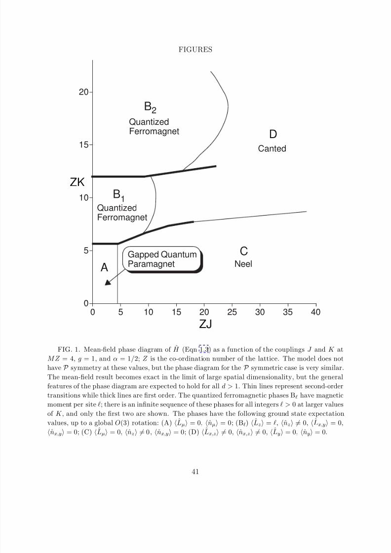
8/3/2019 Subir Sachdev and T. Senthil- Zero temperature phase transitions in quantum Heisenberg ferromagnets
http://slidepdf.com/reader/full/subir-sachdev-and-t-senthil-zero-temperature-phase-transitions-in-quantum 41/45
FIGURES
0
5
10
15
20
0 5 10 15 20 25 30 35 40
ZK
ZJ
B2
B1
QuantizedFerromagnet
QuantizedFerromagnet
A
CNeel
DCanted
Gapped QuantumParamagnet
FIG. 1. Mean-field phase diagram of H (Eqn 1.3) as a function of the couplings J and K at
M Z = 4, g = 1, and α = 1/2; Z is the co-ordination number of the lattice. The model does not
have P symmetry at these values, but the phase diagram for the P symmetric case is very similar.
The mean-field result becomes exact in the limit of large spatial dimensionality, but the general
features of the phase diagram are expected to hold for all d > 1. Thin lines represent second-ordertransitions while thick lines are first order. The quantized ferromagnetic phases B have magnetic
moment per site ; there is an infinite sequence of these phases for all integers > 0 at larger values
of K , and only the first two are shown. The phases have the following ground state expectation
values, up to a global O(3) rotation: (A) Lµ = 0, nµ = 0; (B) Lz = , nz = 0, Lx,y = 0,
nx,y = 0; (C) Lµ = 0, nz = 0, nx,y = 0; (D) Lx,z = 0, nx,z = 0, Ly = 0, ny = 0.
41
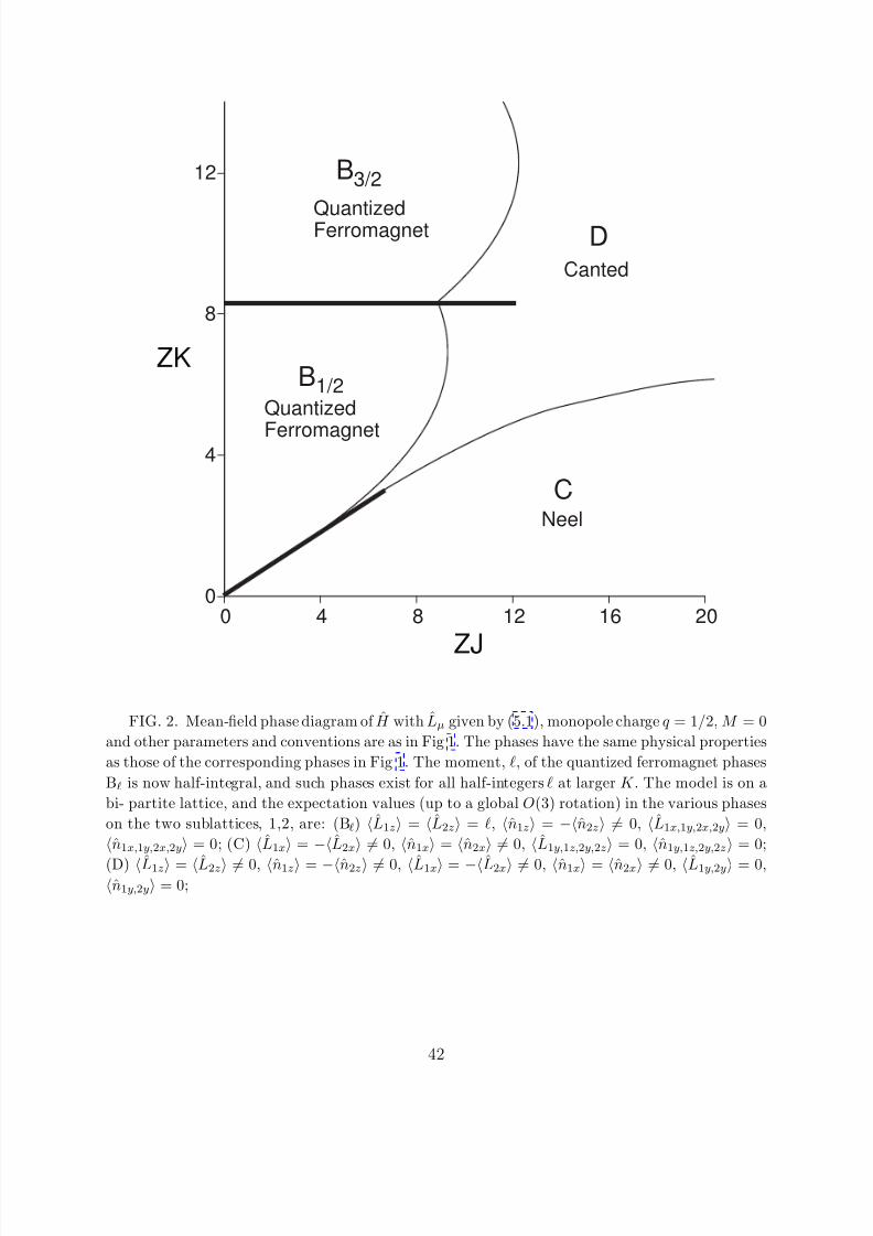
8/3/2019 Subir Sachdev and T. Senthil- Zero temperature phase transitions in quantum Heisenberg ferromagnets
http://slidepdf.com/reader/full/subir-sachdev-and-t-senthil-zero-temperature-phase-transitions-in-quantum 42/45
0
4
8
12
0 4 8 12 16 20
ZK
ZJ
QuantizedFerromagnet
Quantized
Ferromagnet
B1/2
B3/2
CNeel
DCanted
FIG. 2. Mean-field phase diagram of H with Lµ given by (5.1), monopole charge q = 1/2, M = 0
and other parameters and conventions are as in Fig 1. The phases have the same physical properties
as those of the corresponding phases in Fig 1. The moment, , of the quantized ferromagnet phases
B is now half-integral, and such phases exist for all half-integers at larger K . The model is on a
bi- partite lattice, and the expectation values (up to a global O(3) rotation) in the various phases
on the two sublattices, 1,2, are: (B) L1z = L2z = , n1z = −n2z = 0, L1x,1y,2x,2y = 0,
n1x,1y,2x,2y = 0; (C) L1x = −L2x = 0, n1x = n2x = 0, L1y,1z,2y,2z = 0, n1y,1z,2y,2z = 0;
(D) L1z = L2z = 0, n1z = −n2z = 0, L1x = −L2x = 0, n1x = n2x = 0, L1y,2y = 0,n1y,2y = 0;
42
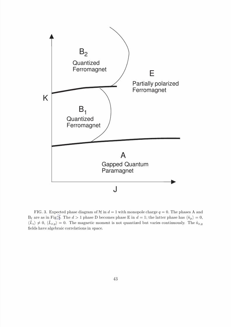
8/3/2019 Subir Sachdev and T. Senthil- Zero temperature phase transitions in quantum Heisenberg ferromagnets
http://slidepdf.com/reader/full/subir-sachdev-and-t-senthil-zero-temperature-phase-transitions-in-quantum 43/45
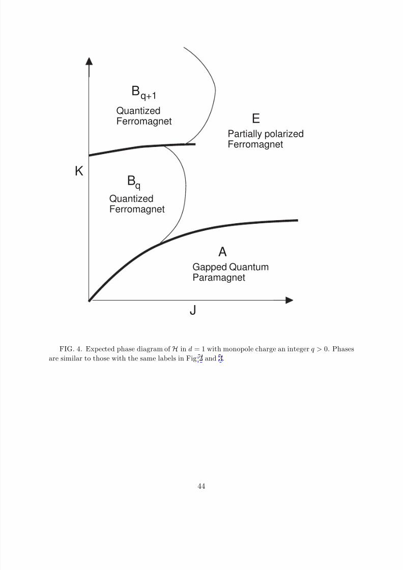
8/3/2019 Subir Sachdev and T. Senthil- Zero temperature phase transitions in quantum Heisenberg ferromagnets
http://slidepdf.com/reader/full/subir-sachdev-and-t-senthil-zero-temperature-phase-transitions-in-quantum 44/45
J
K
AGapped QuantumParamagnet
EPartially polarizedFerromagnet
QuantizedFerromagnet
QuantizedFerromagnet
Bq+1
Bq
FIG. 4. Expected phase diagram of H in d = 1 with monopole charge an integer q > 0. Phases
are similar to those with the same labels in Fig 2 and 3.
44
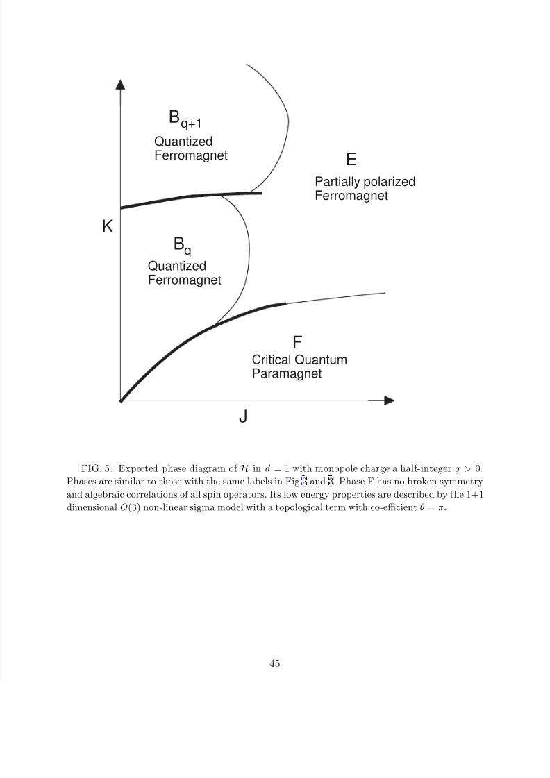
8/3/2019 Subir Sachdev and T. Senthil- Zero temperature phase transitions in quantum Heisenberg ferromagnets
http://slidepdf.com/reader/full/subir-sachdev-and-t-senthil-zero-temperature-phase-transitions-in-quantum 45/45
J
K
FCritical QuantumParamagnet
E
Partially polarizedFerromagnet
QuantizedFerromagnet
QuantizedFerromagnet
Bq
Bq+1
FIG. 5. Expected phase diagram of H in d = 1 with monopole charge a half-integer q > 0.
Phases are similar to those with the same labels in Fig 2 and 3. Phase F has no broken symmetry
and algebraic correlations of all spin operators. Its low energy properties are described by the 1+1
dimensional O(3) non-linear sigma model with a topological term with co-efficient θ = π.