STYLIZED FACTS OF FINANCIAL TIME SERIES: A COMPREHENSIVE ...€¦ · STYLIZED FACTS OF FINANCIAL...

@IJRTER-2017, All Rights Reserved 302

STYLIZED FACTS OF FINANCIAL TIME

SERIES: A COMPREHENSIVE ANALYSIS Mr. Karthik Jillaa Dr. Sarat Chandra Nayakb, Ms. Archana Bathulac

acAssistant Professor bProfessor a,cCMR College of Engineering & Technology, Department of Computer Science and Engineering, Kandlakoya,

Medchal Dist, Hyderabad, India, 501401. bKommuri Pratap Reddy Institute of Technology, Department of Computer Science and Engineering, Ghatkesar,

Medchal Dist, Hyderabad, India, 500088.

Abstract— This article describes a set of stylized

empirical facts emerging from the statistical analysis of

various types of financial time series. The purpose of

this article is to examine some fundamental statistical

behavior of financial time series as well as nonlinearity

associated with them. The knowledge of such facts could

be helpful to establish better empirical models, which is

nonlinear most of the times, in order to produce reliable

forecasts. Also, it illustrates the importance of

stationarity in financial time series analysis and the

concepts behind the most used statistical tests for

checking the stationarity of a series such as Augmented

Dickey – Fuller Test and Phillips-Perron Test, using ten

fast growing stock market indices across the globe.

After observing the principal stylized facts of returns of

a given asset for the empirical financial data, could be in

a more comfortable situation to choose a proper model

for better forecast.

Keywords— financial time series; stylized facts of

financial time series; stationarity; Augmented Dickey –

Fuller Test; Phillips-Perron Test.

I. INTRODUCTION

Financial time series are continually brought the

attention of individual, private and corporate

investors, businessmen, anyone involved in

international trade and the brokers and analysts. Daily

news reports in newspapers, television and radio

inform us for illustration of the latest stock market

index values, currency exchange rates, electricity

prices, and interest rates. It is often desirable to keep

an eye on price behavior frequently and to try to

understand the probable development of the prices in

the future. Many traders deal with the risks associated

with changes in prices. These risks can frequently be

summarized by the variances of future returns,

directly, or by their relationship with relevant co

variances in a portfolio context.

Usually, a time series is defined as a sequence of

values/data points/events separated/occurred by equal

interval of time. A time series can be represented as a

set of discrete values {x1, x2, x3, ⋯ ⋯ , xN} where N

is the total number of observations. A time series

possess both deterministic as well as stochastic

components characterized by noise interference.

However financial time series data is prone to random

fluctuations as compared to ordinary time series. It is

characterized with high nonlinearity, non-stationary

and chaotic in nature. It is often desirable to monitor

price behavior frequently and to try to understand the

probable development of the prices in the future.

The observations or empirical findings common

across a wide range of instruments, markets, and time

periods are called as stylized facts. They can be

obtained by taking a common denominator among the

properties observed in studies of different markets

and instruments [1]. Stylized facts are usually

formulated in terms of qualitative properties of asset

returns and may not be precise enough to distinguish

among different parametric models. The intension

here is not to go the details of stylized facts, rather to

study some of those for the financial time series

considered, which could be helpful to establish better

empirical models by the researchers in this domain.

For more exhaustive study about stylized facts of

financial time series, prospective readers may refer to

the articles in [2-6].

The concept of stationarity has always been essential

to econometric time series analysis, since most

financial time series analysis necessitates that data be

made stationary before any regressions can be

performed. In applied econometric analysis

concerning time series data, the prerequisite of

stationarity is a well-known conception. A stationary

time series is represented by data over time whose

statistical properties remain constant regardless of a

change in the time origin [7]. A financial time series

can be represented by historical stock prices. Earlier

research conducted on financial markets behavior

suggests that financial time series follow a random


walk [8] and the process is inherently non-stationary

because of the presence of a unit root [9]. When a

time series contains a unit root it is essential to

difference the time series to render it stationary [10].

The objective of this study is to examine some

fundamental statistical behavior of financial time

series as well as nonlinearity associated with them.

The knowledge of such facts could be helpful to

establish better empirical models, which is nonlinear

most of the times, to produce reliable forecasts.

Section II discusses some of the stylized facts

exhibited by the financial time series. The importance

of stationarity in financial data is discussed in section

III. Section IV gives the concluding remarks followed

by a list of references.

II. SOME STYLIZED FACTS IN FINANCIAL TIME

SERIES

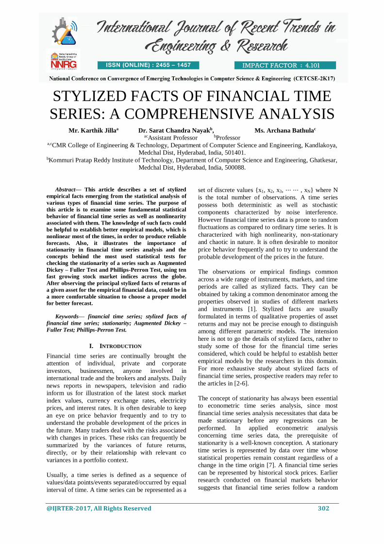
In this article the daily closing prices of ten fast

growing stock markets such as BSE, DJIA,

NASDAQ, FTSE, TAIEX, S&P 500, ASX, LSE,

SSE, and NIKKEI for period of fifteen years (01 Jan.

2000 to 31 Dec. 2014) are used. The daily closing

prices are forming time series, specially called as

financial time series. Figure 1 shows the daily closing

indices of the stock market data used.

Figure 1- Daily observations of closing prices of markets (left)

from top to bottom DJIA, BSE, S&P 500, LSE, NIKKEI and (right)

from top to bottom NASDAQ, FTSE, TAIEX, ASX, and SSE from

January 2000 to December 2014.

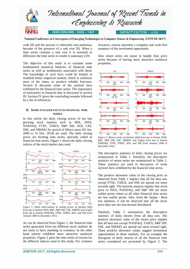
As can be observed from Figure 1, the financial time

series generated from ten different stock markets do

not seem to have anything in common. In the other

hand returns exhibited more attractive statistical

properties. Figure 2 plots the time series of returns for

the different indexes used in this study. For common

investors, returns represent a complete and scale-free

summary of the investment opportunity.

Also return series are easier to handle than price

series because of having more attractive statistical

properties.

Figure 2- Return series of markets (left) from top to bottom DJIA,

BSE, S&P 500, LSE, NIKKEI and (right) from top to bottom

NASDAQ, FTSE, TAIEX, ASX, and SSE from January 2000 to

December 2014.

The descriptive statistics of daily closing prices are

summarized in Table 1. Similarly, the descriptive

statistics of return series are summarized in Table 2.

These statistics are used in discussion of some

stylized facts exhibited by the financial time series.

The positive skewness value of the closing price as

observed from Table 1 implies that all the data sets

except FTSE, TAIEX, and SSE are spread out more

towards right. The kurtosis analysis implies that stock

price of DJIA, NASDAQ, and S&P 500 are more

outlier prone where as all other financial time series

are less outlier prone. Also, from the Jarque - Bera

test statistics, it can be observed that all the stock

price data sets are non-normal distributed.

Similarly Table 2 summarizes the descriptive

statistics of daily returns from all data sets. The

positive skewness value of the return price implies

that all data sets except NASDAQ, TAIEX, S&P 500,

SSE, and NIKKEI are spread out more toward right.

These positive skewness values suggest investment

opportunities in these markets. For an example the

histogram of daily returns of all the financial time

series considered are presented by Figure 3. The


peaks of the histograms are much higher than the

corresponding to the normal distribution and it is

slightly skewed to the right in case of BSE and

slightly skewed to the left in case of NASDAQ stock

data. The kurtosis analysis implies that stock price of

all data sets are more outlier prone than the normal

distribution. Again from the Jarque-Bera test

statistics, it can be observed that all the stock price

data sets are non-normal distributed.

Figure 3 - Histogram of daily returns of all financial time series

against the theoretical normal distribution

Table 1- Descriptive statistics of daily closing prices for ten

different financial time series

Table 2- Descriptive statistics of daily returns for ten different

financial time series

• Gain/Loss Asymmetry

This is a stylized fact in financial time series where

one observes large draw downs in stock index values

but not equally large upward movements. The

skewness of a financial time series is a measure of the

asymmetry of the distribution of the series. It may be

noted that all symmetric distributions including the

normal distribution posses skewnees value equal to

zero. As observed from the return statistics presented

in Table 2, BSE, DJIA, FTSE, LSE, and ASX have

positive skewness values which might point to

possible investment opportunities in these emerging

markets. Positive skewness implies that the right tail

of the distribution is fatter than the left tail which

indicates that positive returns tend to occur more

often than large negative returns. Interested readers

may refer [1, 5].

• Fat tails

The fact that the distribution of stock returns is fat-

tailed has important implications in financial time

series analysis. Since the probability of observing

extreme values is higher for fat-tail distributions

compared to normal distributions, it leads to a gross

underestimation of risk. A random variable is said to

possessing fat tails if it exhibits more extreme

outcomes than a normally distributed random variable

with the same mean and variance [2]. This indicates

that the stock market has more relatively large and

small outcomes than one would expect under the

normal distribution.

The degree of peakedness of a distribution relative to

its tails is measured by its kurtosis value. The normal

distribution has kurtosis value 3. Higher kurtosis

value (leptokurtosis) is a signal of fat tails, means that

most of the variance is due to infrequent extreme

deviations than predicted by the normal distribution.

As observed from Table 2, all the stock data sets have

excess kurtosis which establishes the fact of fat tails

and evidence against normality.

The commonly used graphical method for analyzing

the tails of a distribution is the Quantile - Quantile

(QQ) plot. For an example, the QQ plots for

NASDAQ, BSE, DJIA, and FTSE are presented by

Figure 4. From this it can be observed that returns

have fatter tails to fit the normal distribution.


Figure 4- QQ plot of NASDAQ, BSE, DJIA, and FTSE financial

time series data

• Slow decay of autocorrelation in returns

This fact tells that the autocorrelation function of

absolute returns decays slowly as a function of the

time lag. It is a well-known fact that price movements

in markets do not exhibit any significant linear

autocorrelation

[1]. The autocorrelation function measures how

returns on a given day are correlated with returns on

previous days. If such correlations are statistically

significant, there is strong evidence for predictability.

From Figure 5, it can be clearly seen that the

autocorrelation function for BSE rapidly decays to

zero after a lag.

Figure 5 - Autocorrelation plot of BSE returns, along with a 95%

confidence interval, for the first 20 lags

• Volatility clustering

This is a well-known stylized fact where different

measures of volatility display a positive

autocorrelation over several days, which quantifies

the fact that high-volatility events tend to cluster in

time [1]. This implies that large price variations are

more likely to be followed by large price variations;

hence returns are not random walk.

Figure 6 - Autocorrelation plots of daily BSE returns (top),

absolute returns (middle) and squared Returns (bottom) for first

1000 lags.

Figure 6 shows the autocorrelation function for BSE

return series (top), absolute return (middle), and

Squared returns (bottom). In the top panel most of the

autocorrelations lie within the interval. However in

case of absolute return and squared return the

autocorrelation function is significant even at long

lags which provide the evidence for the predictability.

The lag plots of returns of a day rt against returns of

previous day rt-1is another possible way to

characterize the stylized fact of volatility/return

cluster. For an example, the lag plots corresponding

to returns of DJIA and NASDAQ are shown in the

Figure 7.

A stylized fact that can be observed from such lag

plots is that large returns tend to occur in clusters, i.e.,

it appears that relatively volatile periods characterized

by large returns alternate with more stable periods in

which returns remain small.


Figure 7 - Lag plots of the returns on the DJIA (left) and NASDAQ

(right), on day t, against the return on day t-1

We studied some stylized facts exhibited by ten

different financial time series in the above sub

sections. The following observations can be drawn

from the above analysis.

• We showed that the probability density function

of the return series of these stock indices are skewed

and fat tailed.

• The positive skewness shown by BSE, DJIA,

FTSE, LSE, and ASX return series implying possible

investment opportunities in these markets.

• For all markets, fat tails existed with kurtosis far

in excess of the corresponding to the normal

distribution.

• The linear autocorrelations are insignificant after

a few lags and nonlinear autocorrelations prevailed,

which was evidence for the existence of volatility

clusters.

These preliminary analyses of the stylized facts in

financial time series could be helpful to the

researchers to develop sophisticated and more

accurate model for forecasting stock market behavior.

III. STATIONARITY OF FINANCIAL TIME SERIES

The terms non-stationary and stationary form a

fundamental part of time series econometric analysis.

A stationary time series refers to data whose

statistical properties remain unchanged over time

regardless of the change in time [7].Testing

stationarity in financial time series involves testing

for the order of integration in the time series. It is the

test process to check whether the time series possess

a unit root. There are two principal tests popular

amongst econometricians for testing the null-

hypothesis of a unit root to establish stationarity.

These are the Augmented Dickey-Fuller (ADF) test

for unit roots and the Phillips - Perron(PP) test [11].

There are also several tests for testing stationarity

with stationarity as the null-hypothesis. This article

discusses the outputs from ADF test and PP test

conducted over the ten financial time series.

It is worth mentioning that stationarity of a financial

time series is an important feature which is required

to make statements about the future in order to get

valid forecast. Therefore, the first thing done is to

investigate the time series for the presence of a unit

root to determine whether the analyzed time series is

stationary or not. In case of the standard Dickey-

Fuller test the assumptions to be checked can be

written as follows:

The value of the statistics is calculated and then

compared with the critical values of the ADF test. If

the value of the statistics is less than critical value,

then we reject the null hypothesis, so there is no unit

root and the time series is stationary. An alternative to

the ADF test is Phillips - Perron test (PP test) which

is a non-parametric method and very similar to ADF

test. The only difference between them is that the PP

test allows residues to be auto-correlated by

introducing an automatic correction in the testing

procedure. The mathematical detail of these test are

beyond the scope of this article. We used the ADF

test and PP test available in the Matlab software for

checking the time series stationarity. The outputs

from these tests are summarized in Table-3.

The analysis revealed non - stationarity in levels and

stationarity in first difference for all ten analyzed time

series by applying the Augmented Dickey-Fuller and

Phillips-Perron tests. This may be observed clearly

from the Table-3 presented above. This conclusion is


agreed with the Box –Jenkins approach for modeling

time series stated that financial time series are non-

stationary.

Also, for BSE index prices it can be observed very

high autocorrelations for the first two lags, 1.0000

and 0.9988 respectively. This values decreasing

slowly for the next lags, reaching a value of 0.9602 at

the 30th lag. Also, daily DJIA index prices

correlogram points out very high autocorrelations for

the first two lags, 1.0000 and 0.9985 respectively,

with values decreasing very slowly for the next lags,

reaching a value of 0.9372 at the 30th lag.

Similar observations recorded for NASDAQ, FTSE,

and TAIEX time series. This leads to the conclusion

that the price series of the five stock indices are non-

stationary. On the other hand, high values of Q-Stat

test and zero probability to all lags confirms the

presence of autocorrelation.

Table-3 The output of Augmented Dickey-Fuller test and

Phillips - Perron test for all financial time series data

IV. CONCLUSIONS

This article analyzed some important stylized facts of

ten different financial time series data such as BSE,

JIA, NASDAQ, FTSE, TAIEX, S&P 500, ASX, LSE,

SSE, and NIKKEI for a period of fifteen years. The

description emphasizes properties widespread to a

wide variety of emerging and developing stock

markets across the globe. We observed that, it is

helpful to get aware with the empirical data before

looking for the suitable models. Study of such

stylized facts could be the foundation for nonlinear

modeling of financial assets returns. We discussed the

importance of stationarity as an essential feature

necessary to be achieved before analyzing a financial

time series. The analysis revealed non-stationarity in

levels and stationarity in first difference for all ten

financial time series analyzed. This fact agreed with

the Box – Jenkins approach stated that financial time

series are non - stationary. The knowledge of such

observations could be helpful to establish better

empirical models, which is nonlinear most of the

times, in order to produce reliable forecasts. The

future work may concentrate on developing some

sophisticated nonlinear financial forecasting models.

REFERENCES

[1] R. Cont, (2001),’ Empirical properties of asset returns: stylized facts

and statistical issues’, Quantitative Finance, vol. 1, pp. 223-236.

[2] J. Danielsson, (2011), ‘Financial Risk Forecasting’, Wiley.

[3] M. Sewell, (2011), ‘Characterization of Financial Time Series’,

UCL Department of Computer Science, Research Note.

[4] S. Taylor, (2007), ‘Asset Price Dynamics, Volatility, and Prediction’.

Princeton University Press.

[5] P. Franses, and D. van Dijk, (2000), ‘Non-linear time series models in

empirical finance’, Cambridge University Press.

[6] S. C. Nayak, Misra, B. B., and Behera, H. S. (2017), ‘Efficient

financial time series prediction with evolutionary virtual data position

exploration’, Neural Computing and Applications,

https://doi.org/10.1007/s00521-017-3061-1.

[7] B.D. Fielitz, (1971), ‘Stationarity of random data: Some implications

for the distribution of stock price changes’. Journal of Financial and

Quantitative Analysis, 6(3):1025-1034.

[8] E.F. Fama, (1970), ‘Efficient capital markets: A review

of theory and empirical work’. The Jour-nal of Finance, 25(2):383-

417. May.

[9] S.P. Burke, and J. Hunter, (2005), ‘Modelling non-stationary

economic time series: A multivariate approach’. New York: Palgrave

MacMillan. 253 p.

[10] G.E.P. Box, and G.E.M. Jenkins, (1976), ‘Time series analysis:

Forecasting and control’. San Fran-cisco: Holden Day. 575 p.

[11] D. Asteriou, and S.G. Hall, (2007), ‘Applied econometrics: a modern

approach’. New York: Pal-grave Macmillan. 397 p.

STYLIZED FACTS OF FINANCIAL TIME SERIES: A COMPREHENSIVE ...€¦ · STYLIZED FACTS OF FINANCIAL...

Documents

Transcript of STYLIZED FACTS OF FINANCIAL TIME SERIES: A COMPREHENSIVE ...€¦ · STYLIZED FACTS OF FINANCIAL...