Studyofsoillayeringeﬁectson lateralloadingbehaviorofpilessokocalo.engr.ucdavis.edu/~jeremic/ ·...

in print: ASCE Journal of Geotechnical and Geoenvironmental Engineering.

Study of soil layering effects on

lateral loading behavior of piles

Zhaohui Yang 1 and Boris Jeremic 2

Abstract

This paper presents results of the finite element study on the behavior of a single

pile in elastic–plastic soils. Pile behavior in uniform sand and clay soils as well as cases

with sand layer in clay deposit and clay layer in sand deposit were analyzed using finite

element modeling. Finite element results were used to generate p− y response curves,

which were cross compared to investigate the soil layering effects.

Introduction

The theory of beams on a Winkler-type subgrade (Hartog [1952] ), also known as the p–

y approach, has been widely used to design piles subjected to lateral loading. Based on

that theory, the method models the lateral soil–foundation interaction with empirically de-

rived nonlinear springs (p–y curves). The advancement of computer technology has made

it possible to study this problem using more rigorous elastic–plastic Finite Element Method

(FEM).

Here mentioned are a few representative examples of finite element studies of pile foun-

dations. Muqtadir and Desai [1986] studied the behavior of a pile–group using a three

dimensional (3D) program with nonlinear elastic soil model. An axisymmetric model with

elastic-perfectly plastic soil was used by Pressley and Poulos [1986] to study group effects.

Brown and Shie [1990b], Brown and Shie [1990a], Brown and Shie [1991], and Trochanis

1Department of Civil Engineering, University of Alaska Anchorage, 3211 Providence Drive, Anchorage, AK 99508, Phone:

(907)786-6431, Fax: (907)786-1079, Email: [email protected] of Civil and Environmental Engineering, University of California, One Shields Ave., Davis, CA 95616, Phone:

(530)754-9248, Fax: (530)752-7872, Email: [email protected].

1

et al. [1991] conducted a series of 3D FEM studies on the behavior of a single pile and a pile

group with elastic-plastic soil model. These researchers used interface elements to account

for pile–soil separation and slippage. Moreover, Brown and Shie derived p–y curves from

FEM data, which provide some comparison of the FEM results with the empirical design

procedures in use. Kimura et al. [1995] conducted 3D FEM analysis of the ultimate behavior

of laterally loaded pile groups in layered soil profiles with the soil modeled by Drucker–Prager

model and pile modeled by nonlinear beam elements. A number of model tests of free– or

fixed–headed pile groups under lateral loading in homogeneous soil profiles have been sim-

ulated by Wakai et al. [1999] using 3D elasto-plastic FEM. Pan et al. [2002] studied the

performance of single piles embedded in soft clay under lateral soil movements. A good

correlation between the experiments and the analysis has been observed in these studies.

All these results demonstrated that FEM can capture the essential aspects of the nonlinear

problem.

Information about the lateral behavior of piles in layered soil profiles is very limited.

Some analytical studies have been conducted by Davisson and Gill [1963] and Lee and

Karunaratne [1987] to define the influence of pile length, the thickness of upper layer and

the ratio of stiffness ratio of adjacent layers on the pile response based on the assumption

that the soil is elastic. Reese et al. [1981] conducted small scale laboratory tests on a 25 mm

diameter pile and a field test with 152 mm diameter pile in layered soils and found that there

was a relatively good agreement between deflections measured in the tests and deflections

computed using homogeneous p–y curves at small loads. Georgiadis [1983] proposed an

approach which is currently used in the LPILE program (Reese et al. [2000a,b]). This method

assumes the p–y curves of the first layer are the same as those for homogeneous soils. The

effects of upper layers on the p–y curves of the lower layers are accounted for by the equivalent

depth of the overlying layers based on strength parameters.

To the Authors’ knowledge, there is no literature reporting on FEM study of layering

effects on the behavior of laterally loaded piles in layered profiles. However, it is of great

interest to investigate the layering effects since in practice, most of soil deposits are layered

systems. In a predominantly clay site with a minor sand layer, the sand layer will still be

counted on to provide most of the soil resistance. In this case, the layering effects (probably

reduction of resistance in the sand layer) must be considered. Current practice is to “make

an educated guess to reduce the sand p–y curves to account for the soil layering effects” (Lam

and Law [1996]). Obviously, an educated guess might not result in optimal design. It is very

important to find out how these layers in the layered system affect each other in order to

carry out a more accurate analysis of pile foundation and therefore provide a more effective

2

way for the design of pile foundations in layered soil systems.

This paper describes four 3D finite element models of a laterally loaded pile embedded

in uniform and layered soil profiles, with the dimensions and soil parameters similar to those

used in the centrifuge studies by McVay et al. [1998] and Limin Zhang and Lai [1999]. Visu-

alization tool Joey3D (Yang [2002]) was used to compute the bending moment, shear force and

lateral resistance diagrams along the pile. Model calibration, comparison of finite-element

analysis results with those from centrifuge tests and the LPILE program, and comparison of

finite-element generated p–y curves with traditional p–y curves are summarized in a sepa-

rate paper (Yang and Jeremic [2003]. In this paper, p–y curves from each model were cross

compared to illustrate both the effects of an intermediate soft clay (or sand) layer on the

p–y curves of the sand (or soft clay) layers and the effects of sand (or soft clay) layers on the

intermediate soft clay (or sand) layer. In addition, a limited parametric study was conducted

to further investigate the layering effects in terms of lateral resistance ratios. The OpenSees

OpenSees Development Team (Open Source Project) [1998-2003] finite element framework

was employed for all the computations. Soil modeling was performed using the Template

Elasto–Plastic Framework (Jeremic and Yang [2002]) and solid elements while the piles were

modeled using linear elastic solid elements, all developed by the Authors.

Finite Element Pile Models

Single pile finite element models with the dimensions similar to the prototype model de-

scribed in the above centrifuge tests were developed and a number of static pushover tests

were simulated with 3D FEM using uniform soil and layered soil cases. The models for all

cases were illustrated in Figure 1 (a). There are four main analysis models. Two of them are

dealing with uniform sand and clay deposits, while the other two are featuring layered soil

deposits. In particular, model # 1 has a uniform soft clay deposit, model # 2 includes top

and bottom layers of soft clay with an interlayer of medium dense sand. Model # 3 features

uniform medium dense sand deposit, while model # 4 features top and bottom layers of

medium dense sand with an interlayer of soft clay.

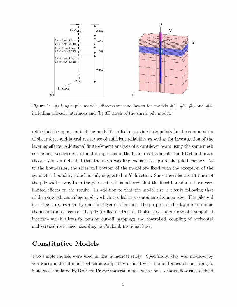
Figure 1 (b) shows the finite element mesh for all four models. Based on symmetry, only

half of the model is meshed. Twenty–node brick elements are used to mesh the soil, pile and

pile–soil interface. The square pile, with a width of 0.429 m and length of 13.7 m1, is divided

into four elastic elements (per cross section) with the properties of aluminum. The mesh is

1All dimensions are from the centrifuge study, prototype scale.

3

a)

��

��

1.72m

1.72m

7.86m

0.429m 2.40m

Interface

Case 3&4: SandCase 1&2: Clay

Case 1&2: ClayCase 3&4: Sand

Case 2&3: SandCase 1&4: Clay

b)

Figure 1: (a) Single pile models, dimensions and layers for models #1, #2, #3 and #4,

including pile-soil interfaces and (b) 3D mesh of the single pile model.

refined at the upper part of the model in order to provide data points for the computation

of shear force and lateral resistance of sufficient reliability as well as for investigation of the

layering effects. Additional finite element analysis of a cantilever beam using the same mesh

as the pile was carried out and comparison of the beam displacement from FEM and beam

theory solution indicated that the mesh was fine enough to capture the pile behavior. As

to the boundaries, the sides and bottom of the model are fixed with the exception of the

symmetric boundary, which is only supported in Y direction. Since the sides are 13 times of

the pile width away from the pile center, it is believed that the fixed boundaries have very

limited effects on the results. In addition to that the model size is closely following that

of the physical, centrifuge model, which resided in a container of similar size. The pile–soil

interface is represented by one thin layer of elements. The purpose of this layer is to mimic

the installation effects on the pile (drilled or driven). It also serves a purpose of a simplified

interface which allows for tension cut-off (gapping) and controlled, coupling of horizontal

and vertical resistance according to Coulomb frictional laws.

Constitutive Models

Two simple models were used in this numerical study. Specifically, clay was modeled by

von Mises material model which is completely defined with the undrained shear strength.

Sand was simulated by Drucker–Prager material model with nonassociated flow rule, defined

4

with the friction and dilation angles. The reason for using such simple models is that

the experimental results used in comparison with simulations did specify only very limited

number of material properties for sands. Furthermore, a small number of model parameters

needed by simple models are convenient for parametric study. In both material models,

the Young’s moduli vary with confining pressure, as shown in Eqn. (1) (cf. Janbu [1963],

Duncan and Chang [1970]):

E = Eo

(

p

pa

)a

(1)

where Eo is Young’s Modulus at atmospheric pressure, p is the effective mean normal stresses,

pa is the atmospheric pressure, and a is constant for a given void ratio. In this work, 0.5 was

used.

The following parameters were used for medium dense sand: friction angle φ = 37.1o,

Shear modulus G at a depth of 13.7 m = 8960 kPa (Eo = 17400 kPa), Poisson’s ratio

ν = 0.35 and unit weight γ = 14.50 kN/m3. These parameters were given by Limin Zhang

and Lai [1999]. A dilation angle of ψ = 0o is used in this work (Brown and Shie [1990b]).

The undrained shear strength, Young’s modulus, Poisson’s ratio and unit weight of clay were

chosen to be Cu = 21.7 kPa, E0 = 11000 kPa, ν = 0.45, γ = 11.8 kN/m3, respectively. The

interface elements were simulated by Drucker–Prager model with a friction angle φ = 25o,

and a dilation angle ψ = 0o. All material properties were summarized in Table 1.

Table 1: Material properties of sand, clay, pile and soil–pile interface used in FEM analysis.

Soil Eo (kPa) ν γ (kN/m3) φ (o) ψ (o) Cu (kPa)

Medium dense sand 17400 0.35 14.5 37.1 0 –

Loose sand 16000 0.35 14.1 34.5 0 –

Clay 11000 0.47 11.8 – – 21.7

Pile 69000000 0.33 26.8 – – –

Soil–pile interface Variable Variable Variable 25 0 –

Comparison of p–y Behavior in Uniform and Layered

Soil Deposits

This section presents representative results related to the behavior of piles in uniform and

layered soil deposits. Specifically the p–y response curves derived for 3D FEM results for

5

homogeneous and layered soil deposits are compared with each other to investigate the

layering effects.

Uniform Clay Deposit and Clay Deposit with an Interlayer of Sand.

The p–y curves of uniform clay deposit and clay deposit with a layer of sand were compared

in Figure 2. It is clearly seen that the p–y curve (Z = −3.75D) close to the interface

(Z = − 4D) is significantly different from that in uniform soil profile.

0 5 100

100

200

300

p (k

N/m

)

Z/D= −0.75

0 5 100

100

200

300Z/D= −1.75

0 5 100

100

200

300Z/D= −2.75

0 5 100

100

200

300

p (k

N/m

)

Z/D= −3.75

0 5 100

100

200

300Z/D= −4.76

0 5 100

100

200

300

y (cm)

Z/D= −5.76

0 5 100

100

200

300

y (cm)

p (k

N/m

)

Z/D= −6.76

0 5 100

100

200

300

y (cm)

Z/D= −8.26

Uniform ClayClay−Sand−Clay

Figure 2: Comparison of p–y curves of uniform clay deposit versus clay deposit with an

interlayer of sand (Sand: φ = 37o; Clay: Cu = 21.7 kPa).

In order to measure the magnitude of the effects of the intermediate sand layer on the

lateral resistance of the soft clay layers and vice versa, the ratios of soil lateral resistances in

the layered (p) and uniform models (phomog. model) at several lateral displacements (i.e. 0.5%,

1.0%, 2.0%, 2.5%, 8.0% and 10.0% of pile width D) were computed and plotted against

vertical coordinate (Z) normalized by pile width D in Figures 3 and 42. In addition, the

2The lateral resistance ratio is only shown for the upper clay layer since the resistance corresponding

to large y is not available at larger depth due to the fact that the pile is loaded at the pile head and the

6

results from two more analyses of the same model with different sands (friction angle φ were

varied from 25o to 30o, while originally, the friction angle was set to 37o) were also included

in these figures.

From Figure 3, it is observed that the lateral resistance ratios are independent of friction

angle φ of sand at small lateral displacements ranging from 0.5% to 1.0% of pile width D.

When the lateral displacement is greater than 1.0%, the variation in φ starts to affect the

lateral resistance ratio, as shown in Figure 4.

0.5 1 1.5−9

−8

−7

−6

−5

−4

−3

−2

−1

0Z

/ D

p/phomog. case

y/D = 0.005

CLAY

γ=11.8kN/m3

SAND

γ=14.5kN/m3

CLAY

γ=11.8kN/m3

φ=25o,Eo=17400kPaφ=30o,Eo=17400kPaφ=37o,Eo=17400kPa

0.5 1 1.5−9

−8

−7

−6

−5

−4

−3

−2

−1

0

p/phomog. case

y/D = 0.010

CLAY

γ=11.8kN/m3

SAND

γ=14.5kN/m3

CLAY

γ=11.8kN/m3


Figure 3: Lateral resistance ratio distributions (Clay:Cu = 21.7 kPa,Eo = 11000 kPa) for

sands with various φ at lateral displacements of 0.5% and 1.0% pile width.

Overall, the effect of the sand layer reduces to less than 10% at about one pile width

above the upper sand interface and the lateral resistance ratio at a quarter pile width above

the upper sand interface is 1.3 at lateral deflection of 0.5% pile width. It may be noted that

the two dashed vertical lines in the lateral resistance plots correspond to lateral resistance

ratios of 0.9 and 1.1, indicating ±10% change in lateral resistance. The 10% change will be

used to judge the extent of influence throughout the rest of the paper. The resistance ratio

below the lower sand interface was not processed since the mesh is becoming coarse and the

results are affected by mesh effects and numerical differentiation, and the pile displacements

are very small.

Besides the effect the sand interlayer has on the clay layer, it is interesting to observe

deflection decreases quickly as depth increases. Also due to the limit of space, plots for 2.0%, 2.5% pile

width are not shown in this paper.

7

1 1.5 2 2.5−4.5

−4

−3.5

−3

−2.5

−2

−1.5

−1

−0.5

0

Z /

D

p/phomog. case

y/D = 0.080

CLAY

γ=11.8kN/m3

SAND

γ=14.5kN/m3


1 1.5 2 2.5−4.5

−4

−3.5

−3

−2.5

−2

−1.5

−1

−0.5

0

p/phomog. case

y/D = 0.100

CLAY

γ=11.8kN/m3

SAND

γ=14.5kN/m3


Figure 4: Lateral resistance ratio distributions in clay layer (Cu = 21.7 kPa,Eo =

11000 kPa) for sands with various φ at lateral displacements of 8% and 10% pile width.

in Figure 3 that the soft clay layers also have significant effect on the lateral resistance of

the intermediate sand layer. The lateral resistance ratios are less than 0.9 throughout the

interlayer of sand. Surprisingly, the effects are not symmetric at lateral deflection of 0.5%.

The resistance ratio is 0.85 at 0.25D below the upper sand interface, while that is 0.72 at

0.25D above the lower sand interface. This non–symmetry is probably due to the non–

symmetric deformation3 mode in the pile. As the pile is loaded laterally at the pile head,

the right–hand–side sand close to the pile below certain depth tends to move downward to

the right, which can be observed in Figure 8 (b). Therefore, the sand close to the upper

interface moves against sand, while that close to the lower interface moves against soft

clay. This type of movement results in the larger reduction in resistance at the lower sand

interface than at the upper sand interface. The decrease in lateral resistance is mainly due

to the lower stiffness in the adjacent soft clay layers. In addition, the smaller unit weight

of the soft clay results in smaller mean effective normal stresses in the sand layer than the

homogeneous model, which will reduce the stiffness of the sand and therefore also contribute

to the reduction in lateral resistance at the intermediate sand layer.

3Non–symmetric with respect to the horizontal plane in between the interfaces (midway through the sand

layer).

8

Uniform Sand Deposit and Sand Deposit with an Interlayer of Soft

Clay.

By comparing the p–y curves of uniform sand deposit and sand deposit with an interlayer of

soft clay, it was found that the effect of soft clay on the lateral resistance of sand propagates

further away from the interface than Clay-Sand-Clay case, as described above in section .

In addition to that, it was found that the heave in front of the pile will affect the lateral

resistance of sand at shallow depth. Therefore, for sand deposit with an interlayer of soft

clay, the thickness of upper sand layer was increased from 1.72 m to 2.36 m (the thickness

of the soft clay layer was kept the same) to investigate the range of layering effects. Three

models were analyzed by only varying the undrained shear strength Cu ( i.e. 13.0, 21.7 and

30.3 kPa ) of the soft clay layer.

Similar to the previous analysis, the p–y curves from the uniform deposit and the re-

configured layered deposit were compared in Figure 5 and the lateral resistance ratios at

several lateral displacements (i.e. 0.5%, 1.0%, 2.0%, 2.5%, 5.0% and 6.5% of pile width D )

for all three models were computed and shown in Figures 6 and 7. It may be observed from

Figure 5 that obvious difference may be observed in several p−−y curves further away from

the interface.From Figure 6, it is noted that the effects of the intermediate soft clay layer are also

independent of its undrained shear strength at small lateral displacements ranging from

0.5% D to 1.0% D. When the lateral displacement is greater than 1.0% D, the change in Cu

starts to affect the lateral resistance ratio, as shown in Figure 7. Similar to the Clay–Sand–

Clay model, the effect of the intermediate soft clay layer reduces to less than 10% at one pile

width above the clay interface. The lateral resistance ratio at 0.25D above the clay interface

is about 0.75. For large lateral displacements ranging from 5.0% D to 6.5% D, the 10%

change in lateral resistance extends to 1.5 D - 2 D, as can be observed in Fig. 7. It may be

noted that, at a lateral displacement of 6.5% D, the lateral resistance ratio at 0.25D above

the clay interface changes from 0.58 to 0.67 when Cu increases from 13.0 kPa to 30.3 kPa.

Figures 8 (a) and (b) show the details of displaced models around the interfaces for

the Sand-Clay-Sand and Clay-Sand-Clay profiles, respectively. The deformed model was

overlapped with undeformed model for comparison. Ground heave can be easily observed in

front of the pile from both figures. It is noted from Figure 8 (a) that the sand crosses the

upper clay interface and moves into the intermediate soft clay layer. The movement slightly

strengthens the soft clay soil and partially causes the slight increase of lateral resistance at

the top of soft clay layer. Most importantly, the movement will soften the sand close to the

9

0 5 100

100

200

300

p (k

N/m

)

Z/D= −0.75

0 5 100

100

200

300Z/D= −1.75

0 5 100

100

200

300Z/D= −2.75

0 5 100

100

200

300

p (k

N/m

)

Z/D= −3.75

0 5 100

100

200

300Z/D= −4.76

0 5 100

100

200

300

y (cm)

Z/D= −5.76

0 5 100

100

200

300

y (cm)

p (k

N/m

)

Z/D= −6.76

0 5 100

100

200

300

y (cm)

Z/D= −8.26

Uniform SandSand−Clay−Sand

Figure 5: Comparison of p–y curves for uniform sand deposit versus sand deposit with an

interlayer of soft clay (Sand: φ = 37o; Clay: Cu = 21.7 kPa).

10

0.5 1 1.5−9

−8

−7

−6

−5

−4

−3

−2

−1

0

Z /

D

p / phomog. case

y/D = 0.005

SAND

γ=14.5kN/m3

CLAY

γ=11.8kN/m3

Cu=13.0kPa,Eo=11000kPaCu=21.7kPa,Eo=11000kPaCu=30.3kPa,Eo=11000kPa

0.5 1 1.5−9

−8

−7

−6

−5

−4

−3

−2

−1

0

p / phomog. case

y/D = 0.010

SAND

γ=14.5kN/m3

CLAY

γ=11.8kN/m3


Figure 6: Lateral resistance ratio distributions (Sand:φ = 37o, Eo = 17400 kPa) for clays

with various Cu at lateral displacements of 0.5% and 1.0% pile width.

0.5 0.6 0.7 0.8 0.9 1−6

−5

−4

−3

−2

−1

0

Z /

D

p / phomog. case

y/D = 0.050

SANDγ=14.5kN/m3

CLAY, γ=11.8kN/m3


0.5 0.6 0.7 0.8 0.9 1−6

−5

−4

−3

−2

−1

0

p / phomog. case

y/D = 0.065

SANDγ=14.5kN/m3

CLAY, γ=11.8kN/m3



with various Cu at lateral displacements of 5.0% and 6.5% pile width.

11

upper layer interface, due to the reduction of confinement to the sand. For the Clay-Sand-

Clay profile, the stronger sand layer penetrates into the softer clay layers at both interfaces.

This penetration softens the sand close to both interface, due to the same reason as above.

(a) (b)

Figure 8: Details of displaced model indicating ground heave and movement of soils across

the layer interfaces at lateral load of 400 kN: (a) sand deposit with an interlayer of soft clay

and (b) clay deposit with an interlayer of medium sand. The pile elements are removed so

that the interface layer in the middle can be seen clearly.

Parametric Study for the Lateral Resistance Ratios in

Terms of Stiffness and Strength Parameters.

To further investigate the effects of soil stiffness on the lateral resistance ratios at small

displacement and/or large displacement, further analyses were carried out for the Clay–

Sand–Clay and Sand–Clay–Sand models by changing both stiffness parameter (i.e. Eo) and

strength parameter ( Cu for clay, or φ for sand) using the same finite element models as

above. The model configurations and intermediate layer soil parameters were summarized

in Tables 2 and 3.

Lateral resistance ratios were plotted in Figures 9 and 10 for the Clay–Sand–Clay model,

and in Figures 11 and 12 for the Sand–Clay–Sand model. By comparing Figures 4 and 10 for

pile displacements of 8% D and 10% D, and Figures 7 and 12 for pile displacements of 5%

D and 6.5% D, it is clear that the lateral resistance ratios are almost the same for the upper

12

Table 2: Summary of model configurations and intermediate sand layer parameters for Clay–

Sand–Clay model in the parametric study.

Case Soil Profile Depth of Interfaces Intermediate Sand Layer

Upper Lower Eo (kPa) φ

1 Clay–Sand–Clay -1.72 m -3.43 m 11500 25o



Table 3: Summary of model configurations and intermediate clay layer parameters for Sand–

Clay–Sand model in the parametric study.

Case Soil Profile Depth of Interfaces Intermediate Clay Layer

Upper Lower Eo (kPa) Cu (kPa)

1 Sand–Clay–Sand -2.36 m -4.08 m 8000 13.0

2 Sand–Clay–Sand -2.36 m -4.08 m 11000 21.7

3 Sand–Clay–Sand -2.36 m -4.08 m 12500 30.3

layer soil even if the stiffness parameter Eo of intermediate layer soil was varied by more than

30%. However, the lateral resistance ratios at small displacement (0.5% D and 1.0% D) were

obviously influenced by the variation of Eo, as can be observed by comparing Figures 3 and

9 for the Clay–Sand–Clay model, and Figures 6 and 11 for the Sand–Clay–Sand model. For

medium pile displacements (e.g. 2% D and 2.5% D), both stiffness and strength parameters

have effects on the lateral resistance ratios.

It will be useful to relate the effects of (a) the relative stiffness which controls the lateral

resistance ratio at small lateral displacements and (b) the relative strength which determines

the lateral resistance ratio at large lateral displacements with the lateral resistance ratio. To

exclude the effects of unit weight, only the results above the upper interface in the Sand–

Clay–Sand model are processed. The ratio of Young’s moduli of clay and sand soils was

used to define the relative stiffness Rstiffness of the two layers. On the other hand, the ratio

of largest lateral resistances of uniform clay and sand4 at the upper interface (-2.36 m) was

4It would be better to use the ultimate lateral resistances for both clay and sand to define the relative

strength but these values are not available from the current numerical results since pile displacement y is

not large enough.

13

0.5 1 1.5−9

−8

−7

−6

−5

−4

−3

−2

−1

0

Z /

D

p/phomog. case

y/D = 0.005

CLAY

γ=11.8kN/m3

SAND

γ=14.5kN/m3

CLAY

γ=11.8kN/m3


0.5 1 1.5−9

−8

−7

−6

−5

−4

−3

−2

−1

0

p/phomog. case

y/D = 0.010

CLAY

γ=11.8kN/m3

SAND

γ=14.5kN/m3

CLAY

γ=11.8kN/m3


Figure 9: Lateral resistance ratio distributions (Clay:Cu = 21.7 kPa,Eo = 11000 kPa) for

sands with various φ and Eo at lateral displacements of 0.5% and 1.0% pile width.

1 1.5 2 2.5−4.5

−4

−3.5

−3

−2.5

−2

−1.5

−1

−0.5

0

Z /

D

p/phomog. case

y/D = 0.080

CLAY

γ=11.8kN/m3

SAND

γ=14.5kN/m3


1 1.5 2 2.5−4.5

−4

−3.5

−3

−2.5

−2

−1.5

−1

−0.5

0

p/phomog. case

y/D = 0.100

CLAY

γ=11.8kN/m3

SAND

γ=14.5kN/m3


Figure 10: Lateral resistance ratio distributions in clay layer (Cu = 21.7 kPa,Eo =

11000 kPa) for sands with various φ and Eo at lateral displacements of 8% and 10% pile

width.

14

0.5 1 1.5−9

−8

−7

−6

−5

−4

−3

−2

−1

0

Z /

D

p / phomog. case

y/D = 0.005

SAND

γ=14.5kN/m3

CLAY

γ=11.8kN/m3


0.5 1 1.5−9

−8

−7

−6

−5

−4

−3

−2

−1

0

p / phomog. case

y/D = 0.010

SAND

γ=14.5kN/m3

CLAY

γ=11.8kN/m3


Figure 11: Lateral resistance ratio distributions (Sand:φ = 37o, Eo = 17400 kPa) for inter-

mediate layer of clays with various Cu and Eo at lateral displacements of 0.5% and 1.0% pile

width.

0.5 0.6 0.7 0.8 0.9 1−6

−5

−4

−3

−2

−1

0

Z /

D

p / phomog. case

y/D = 0.050

SANDγ=14.5kN/m3

CLAY, γ=11.8kN/m3


0.5 0.6 0.7 0.8 0.9 1−6

−5

−4

−3

−2

−1

0

p / phomog. case

y/D = 0.065

SANDγ=14.5kN/m3

CLAY, γ=11.8kN/m3



with various Cu and Eo at lateral displacements of 5.0% and 6.5% pile width.

15

used to define the relative strength Rstrength−FEM , as described in Equations (2) and (3).

Rstiffness =Eo−clay

Eo−sand

(2)

Rstrength−FEM =pclay−FEM

psand−FEM

(3)

The lateral resistance ratios at lateral displacement of 6.5% D were plotted against Cu in

Figure 13. For comparison, the relative stiffness Rstiffness and relative strength Rstrength−FEM

were also included in the same plot.

12 14 16 18 20 22 24 26 28 30 320.2

0.4

0.6

0.8

1

Undrained Shear Strength of Soft Clay Cu (kPa)

p / p

hom

og. c

ase a

t def

lect

ion

of 6

.5%

D

Rstiffness

Rstrength−FEM

Distance = 0.25DDistance = 1.25DDistance = 2.25DDistance = 3.25DDistance = 4.25D

Figure 13: Lateral resistance ratios in the upper sand layer (φ = 37o) at various distances

from the interface for pile displacement of 6.5% pile width.

As can be observed from this plot, the lateral resistance ratio decreases from 0.69 to 0.56

almost proportionally as Cu drops from 30 kPa to 13 kPa at 0.25 D above the upper interface,

and the ratio is greater than the relative strengthRstrength−FEM . Since the ultimate resistance

of uniform sand will be larger than the computed largest value (which is still increasing , as

can be observed from Figure 5 at Z=-3.75D) and that of uniform clay almost will almost

remain the same (refer to Figure 2 at Z=-3.75D), this relative strength value will drop and

the above statement still holds. There is certain correlation between the lateral resistance

ratio close to the upper interface and Rstrength−FEM at 6.5%D pile displacement. As the

distance to the upper interface increases, this correlation diminishes. The relative stiffness

curve intercepts with the lateral resistance ratio curves at 0.25D above the upper interface.

16

This implies that the presence of the clay, which is softer than the sand, somehow caused the

layered system to be softer than either of the homogeneous models. This seems illogical, and

in fact previous discussions and comparisons showed that Rstrength−FEM is more important

than Rstiffness at these large relative displacements.

It is also interesting to examine the relationship between the lateral resistance ratio and

the relative variables (i.e. strength and stiffness) when lateral displacement increases, as

presented in Figures 14 and 15. Figure 14 shows that the lateral resistance ratios at 0.25D

12 14 16 18 20 22 24 26 28 30 320.35

0.4

0.45

0.5

0.55

0.6

0.65

0.7

0.75

0.8

0.85


p / p

hom

og. c

ase a

t 0.2

5D a

bove

the

Inte

rfac

e

Deflection = 6.5% DDeflection = 5.0% DDeflection = 4.0% DR

strength−FEMR

stiffness

Figure 14: Lateral resistance ratio at a quarter pile width above the upper clay interface for

various deflections.

above the interface decreases and come closer to the relative strength Rstrength−FEM curve

as the lateral displacement increases from 4.0%D to 6.5%D. The relative stiffness Rstiffness

was also plotted in Figure 14 and it intercepts with the lateral resistance ratio curve, which

has similar implications as the above discussion for Figure 13 and is illogical. On the other

hand, as the lateral displacement decreases from 1.5%D to 0.5% D, the lateral resistance

ratios keep decreasing and come closer to the relative stiffness ratio Rstiffness, as shown in

Figure 15. There is almost a linear relationship between the lateral resistance ratio and the

relative stiffness at small displacements.

From the above analysis, it is safe to say that the lateral resistance ratio is dominated by

the relative stiffness Rstiffness at small displacement (i.e. ≤ 0.5%D), while that is controlled

by the relative strength Rstrength−FEM at large displacement ( i.e. ≥ 4.0%D). For small

17

12 14 16 18 20 22 24 26 28 30 320.4

0.5

0.6

0.7

0.8

0.9

1

1.1

1.2


p / p

hom

og. c

ase a

t 0.2

5D a

bove

the

Inte

rfac

e

Deflection = 1.5% DDeflection = 1.0% DDeflection = 0.5% DR

stiffness

Figure 15: Lateral resistance ratio at one quarter pile width above the upper clay interface

for clays with various Cu and Eo at small pile displacements ranging from 0.5% to 1.5% pile

width.

displacement, the smaller the displacement is, the closer the lateral resistance ratio is to the

relative stiffness; for large displacement, the larger the displacement, the closer the lateral

resistance ratio is to the relative strength.

Figures 16, 17 and 18 summarize observed lateral resistance ratios in layered profiles.

Figure 16 shows the lateral resistance ratios in the intermediate sand layer corresponding

to various relative stiffness Rstiffness at pile displacement of 0.5%D for the Clay–Sand–Clay

model. Figures 17 and 18 show the lateral resistance ratios corresponding to various relative

stiffness Rstiffness and relative strength Rstrength−FEM at pile displacements of 0.5% D and

6.5% D for the Sand–Clay–Sand model. The effects of the intermediate clay layer on the

upper sand layer reduce to less than 10% at a distance of 0.5 to 1.5 D above the interface

at small pile displacement (e.g. 0.5% D), while that effects reduce to less than 10% at a

distance of 1.25 to 2.0 D above the interface at large pile displacement (e.g. 6.5%D).

One may notice that the lateral resistance ratios corresponding to the relative stiffness

Rstiffness = 0.63 in Figures 16 and 17 are not the same. The ratios close to the lower sand

interface in the Clay–Sand–Clay model is slightly larger than that in the Sand–Clay–Sand

model. This difference is due to the fact that the lateral resistance ratios in the intermediate

sand layer also include the effects of smaller unit weight of upper layer clay.

18

0.5 0.6 0.7 0.8 0.9 1 1.1 1.2 1.3 1.4 1.5−9

−8

−7

−6

−5

−4

−3

−2

−1

0

Z /

D

p/phomog. case

y/D = 0.005

CLAY

γ=11.8kN/m3

SAND

γ=14.5kN/m3

CLAY

γ=11.8kN/m3

Rstiffness

= 0.96R

stiffness = 0.81

Rstiffness

= 0.63

Figure 16: Summary of observed lateral resistance ratios from FEM analysis for the Clay–

Sand–Clay profile at small deflection (y/D=0.5%).

0.5 0.6 0.7 0.8 0.9 1 1.1 1.2 1.3 1.4 1.5

−9

−8

−7

−6

−5

−4

−3

−2

−1

0

SAND

γ=14.5kN/m3

CLAY

γ=11.8kN/m3

y/D=0.005

INTERFACE

Z /

D

p / phomog. case

Rstiffness

= 0.46R

stiffness = 0.63

Rstiffness

= 0.72

Figure 17: Summary of observed lateral resistance ratios from FEM analysis for the Sand–

Clay–Sand profile at small deflection (y/D=0.5%).

19

0.5 0.6 0.7 0.8 0.9 1 1.1 1.2 1.3 1.4 1.5

−9

−8

−7

−6

−5

−4

−3

−2

−1

0

SAND

γ=14.5kN/m3

CLAY

γ=11.8kN/m3

y/D=0.065

INTERFACE

p / phomog. case

Rstrength

= 0.39R

strength = 0.48

Rstrength

= 0.65

Figure 18: Summary of observed lateral resistance ratios from FEM analysis for the Sand–

Clay–Sand profile at large deflection (y/D=6.5%).

Summary

This section summarizes results from finite element analysis on the behavior of a single pile

in elastic–plastic layered soils. Based on the results presented, the following conclusions can

be drawn.

1. The layering effects are two–way. Not only the lower layers are affected by the upper

layers, but the upper layers are also affected by the lower layers. Furthermore, the

layering effects are not symmetric. In the case of pile laterally loaded at the pile head,

the effect of an interface extends further into the layer above the interface than it does

into the layer below the interface at small displacements.

2. In the Clay–Sand–Clay model, the lateral resistance of soft clay increases by as much

as 30% and the effect extends to one pile width above the upper sand interface for

Rstiffness = 0.63 at small pile displacement (0.5%D). Nonetheless, the increase of lateral

resistance in the upper clay layer at large pile displacement (8–10%D) extends only one

finite element above the upper sand interface. On the other hand, the clay layers also

have significant effects on the lateral resistance of sand throughout the intermediate

layer.

20

3. In the Sand–Clay–Sand model, the intermediate clay layer has considerable effects on

the lateral resistance of the upper sand layer, and the sand layers also have significant

effects on the lateral resistance of the intermediate clay layer, causing 10 to 40% increase

in its lateral resistance.

4. The lateral resistance ratio is dominated by the relative stiffness at small displacements

(i.e. ≤ 1.0%D), while that is controlled by the relative strength at large displacements

(i.e. ≥ 5.0%D).

It must be pointed out that the above observed lateral resistance ratios may only be

applied to similar stratigraphies, pile deformation modes, and other conditions considered

in this work. Further analyses are needed to investigate the effects of other stratigraphies,

pile deformation modes, pile diameters, and other factors, in order to draw more general

guidelines. Future studies with a refined mesh around the interface will provide better

resolution of the resistance ratio around the interface. Future studies of the effects of the

interface layer on the layering effects will also be very interesting.

Acknowledgment

The authors are grateful to the reviewers’ constructive comments. This work was primarily

supported by the Earthquake Engineering Research Centers Program of the National Science

Foundation under Award Number EEC-9701568.

References

D. A. Brown and C.-F. Shie. Numerical experiments into group effects on the response of

piles to lateral loading. Computers and Geotechnics, 10:211–230, 1990a.

D. A. Brown and C.-F. Shie. Three dimensional finite element model of laterally loaded

piles. Computers and Geotechnics, 10:59–79, 1990b.

D. A. Brown and C.-F. Shie. Some numerical experiments with a three dimensional finite

element model of a laterally loaded pile. Computers and Geotechnics, 12:149–162, 1991.

21

M. T. Davisson and H. L. Gill. Laterally loaded piles in a layered soil system. Journal of

the Soil Mechanics and Foundations Division, 89(SM3):63–94, May 1963. Paper 3509.

J. M. Duncan and C.-Y. Chang. Nonlinear analysis of stress and strain in soils. Journal of

Soil Mechanics and Foundations Division, 96:1629–1653, 1970.

M. Georgiadis. Development of p-y curves for layered soils. In Geotechnical Practice in

Offshore Engineering, pages 536–545. Americal Society of Civil Engineers, April 1983.

J. P. D. Hartog. Advanced Strength of Materials. Dover Publications, Inc., 1952.

N. Janbu. Soil compressibility as determined by odometer and triaxial tests. In Proceedings of

European Conference on Soil Mechanics and Foundation Engineering, pages 19–25, 1963.

B. Jeremic and Z. Yang. Template elastic–plastic computations in ge-

omechanics. International Journal for Numerical and Analytical Methods

in Geomechanics, 26(14):1407–1427, 2002. available as CGM report at:

http://sokocalo.engr.ucdavis.edu/~jeremic/publications/CGM0102.pdf.

M. Kimura, T. Adachi, H. Kamei, and F. Zhang. 3-D finite element analyses of the ul-

timate behavior of laterally loaded cast-in-place concrete piles. In G. N. Pande and

S. Pietruszczak, editors, Proceedings of the Fifth International Symposium on Numerical

Models in Geomechanics, NUMOG V, pages 589–594. A. A. Balkema, September 1995.

I. P. Lam and H. K. Law. Soil–foundation–structure-interaction analytical considerations by

empirical p–y methods. In The fourth Caltrans Seismic Research Workshop, Sacramento,

CA, July 1996. California Dept. of Transportation, Engineering Service Center.

S. L. Lee and G. P. Karunaratne. Laterally loaded piles in layered soil. Soils and Foundations,

27(4):1–10, Dec. 1987.

M. M. Limin Zhang and P. Lai. Numerical analysis of laterally loaded 3x3 to 7x3 pile groups

22

in sands. Journal of Geotechnical and Geoenvironmental Engineering, 125(11):936–946,

Nov. 1999.

M. McVay, L. Zhang, T. Molnit, and P. Lai. Centrifuge testing of large laterally loaded pile

groups in sands. Journal of Geotechnical and Geoenvironmental Engineering, 124(10):

1016–1026, October 1998.

A. Muqtadir and C. S. Desai. Three dimensional analysis of a pile-group foundation. Inter-

national journal for numerical and analysis methods in geomechanics, 10:41–58, 1986.

OpenSees Development Team (Open Source Project). OpenSees: open system for earthquake

engineering simulations. http://opensees.berkeley.edu/, 1998-2003.

J. L. Pan, A. T. C. Goh, K. S. Wong, and A. R. Selby. Three–dimensional analysis of

single pile response to lateral soil movements. International Journal for Numerical and

Analytical Methods in Geomechanics, 26:747–758, 2002.

J. S. Pressley and H. G. Poulos. Finite element analysis of mechanisms of pile group behavior.

International Journal for Numerical and Analytical Methods in Geomechanics, 10:213–221,

1986.

L. C. Reese, J. D. Allen, and J. Q. Hargrove. Laterally loaded piles in layered soils. In

P. C. of X ICSMFE, editor, Proceedings of the Tenth International Conference on Soil

Mechanics and Foundations Engineering, volume 2, pages 819–822, Stockholm, June 1981.

A. A. Balkema.

L. C. Reese, S. T. Wang, W. M. Isenhower, and J. A. Arrellaga. LPILE plus 4.0 Technical

Manual. ENSOFT, INC., Austin, TX, version 4.0 edition, Oct. 2000a.

L. C. Reese, S. T. Wang, I. W. M., A. J. A., and H. J. LPILE plus 4.0 User Guide. ENSOFT,

INC., Austin, TX, version 4.0 edition, Oct. 2000b.

23

A. M. Trochanis, J. Bielak, and P. Christiano. Three-dimensional nonlinear study of piles.

Journal of Geotechnical Engineering, 117(3):429–447, March 1991.

A. Wakai, S. Gose, and K. Ugai. 3-d elasto-plastic finite element analysis of pile foundations

subjected to lateral loading. Soil and Foundations, 39(1):97–111, Feb. 1999.

Z. Yang. Three Dimensional Nonlinear Finite Element Analysis of Soil–Foundation–

Structure Interaction. PhD thesis, University of California at Davis, Davis, California,

September 2002.

Z. Yang and B. Jeremic. Numerical study of the effective stiffness for

pile groups. International Journal for Numerical and Analytical Methods

in Geomechanics, 27(15):1255–1276, Dec 2003. available in preprint at:

http://sokocalo.engr.ucdavis.edu/~jeremic/publications/Piles02.pdf.

24

List of Figures

1 (a) Single pile models, dimensions and layers for models #1, #2, #3 and #4,

including pile-soil interfaces and (b) 3D mesh of the single pile model. . . . . 4

2 Comparison of p–y curves of uniform clay deposit versus clay deposit with an

interlayer of sand (Sand: φ = 37o; Clay: Cu = 21.7 kPa). . . . . . . . . . . 6

3 Lateral resistance ratio distributions (Clay:Cu = 21.7 kPa,Eo = 11000 kPa)

for sands with various φ at lateral displacements of 0.5% and 1.0% pile width. 7

4 Lateral resistance ratio distributions in clay layer (Cu = 21.7 kPa,Eo =

11000 kPa) for sands with various φ at lateral displacements of 8% and 10%

pile width. . . . . . . . . . . . . . . . . . . . . . . . . . . . . . . . . . . . . . 8

5 Comparison of p–y curves for uniform sand deposit versus sand deposit with

an interlayer of soft clay (Sand: φ = 37o; Clay: Cu = 21.7 kPa). . . . . . . . 10

6 Lateral resistance ratio distributions (Sand:φ = 37o, Eo = 17400 kPa) for

clays with various Cu at lateral displacements of 0.5% and 1.0% pile width. . 11


clays with various Cu at lateral displacements of 5.0% and 6.5% pile width. . 11

8 Details of displaced model indicating ground heave and movement of soils

across the layer interfaces at lateral load of 400 kN: (a) sand deposit with an

interlayer of soft clay and (b) clay deposit with an interlayer of medium sand.

The pile elements are removed so that the interface layer in the middle can

be seen clearly. . . . . . . . . . . . . . . . . . . . . . . . . . . . . . . . . . . 12

25

9 Lateral resistance ratio distributions (Clay:Cu = 21.7 kPa,Eo = 11000 kPa)

for sands with various φ and Eo at lateral displacements of 0.5% and 1.0%

pile width. . . . . . . . . . . . . . . . . . . . . . . . . . . . . . . . . . . . . . 14

10 Lateral resistance ratio distributions in clay layer (Cu = 21.7 kPa,Eo =

11000 kPa) for sands with various φ and Eo at lateral displacements of 8%

and 10% pile width. . . . . . . . . . . . . . . . . . . . . . . . . . . . . . . . . 14


intermediate layer of clays with various Cu and Eo at lateral displacements of

0.5% and 1.0% pile width. . . . . . . . . . . . . . . . . . . . . . . . . . . . . 15


clays with various Cu and Eo at lateral displacements of 5.0% and 6.5% pile

width. . . . . . . . . . . . . . . . . . . . . . . . . . . . . . . . . . . . . . . . 15

13 Lateral resistance ratios in the upper sand layer (φ = 37o) at various distances

from the interface for pile displacement of 6.5% pile width. . . . . . . . . . . 16

14 Lateral resistance ratio at a quarter pile width above the upper clay interface

for various deflections. . . . . . . . . . . . . . . . . . . . . . . . . . . . . . . 17

15 Lateral resistance ratio at one quarter pile width above the upper clay interface

for clays with various Cu and Eo at small pile displacements ranging from 0.5%

to 1.5% pile width. . . . . . . . . . . . . . . . . . . . . . . . . . . . . . . . . 18

16 Summary of observed lateral resistance ratios from FEM analysis for the Clay–

Sand–Clay profile at small deflection (y/D=0.5%). . . . . . . . . . . . . . . . 19

17 Summary of observed lateral resistance ratios from FEM analysis for the

Sand–Clay–Sand profile at small deflection (y/D=0.5%). . . . . . . . . . . . 19

26

18 Summary of observed lateral resistance ratios from FEM analysis for the

Sand–Clay–Sand profile at large deflection (y/D=6.5%). . . . . . . . . . . . 20

27

List of Tables

1 Material properties of sand, clay, pile and soil–pile interface used in FEM

analysis. . . . . . . . . . . . . . . . . . . . . . . . . . . . . . . . . . . . . . . 5

2 Summary of model configurations and intermediate sand layer parameters for

Clay–Sand–Clay model in the parametric study. . . . . . . . . . . . . . . . . 13

3 Summary of model configurations and intermediate clay layer parameters for

Sand–Clay–Sand model in the parametric study. . . . . . . . . . . . . . . . . 13

28

Studyofsoillayeringeﬁectson lateralloadingbehaviorofpilessokocalo.engr.ucdavis.edu/~jeremic/ ·...

Documents

Transcript of Studyofsoillayeringeﬁectson lateralloadingbehaviorofpilessokocalo.engr.ucdavis.edu/~jeremic/ ·...