Structures Lab 1

Cantilever Beam Vibration Test

David Clark

Group 1

MAE 449 – Aerospace Laboratory

2 | P a g e

Abstract

The following exercise observes the lateral modes of vibration of a thin steel cantilever specimen.

Using accurate geometric and material properties, the natural frequency response for the cantilever

beam can be calculated. For the steel beam used in the experiment, the first natural response was

approximately 8.5 Hz. The experimental error experienced at low frequencies was as much as 50%,

however at high frequencies, the error was only 5%.

3 | P a g e

Contents

Abstract .................................................................................................................................................. 2

Introduction and Background ................................................................................................................. 4

Introduction ........................................................................................................................................ 4

Equipment and Procedure ..................................................................................................................... 6

Equipment .......................................................................................................................................... 6

Experiment Setup ............................................................................................................................... 6

Basic Procedure .................................................................................................................................. 6

Data, Calculations, and Analysis ............................................................................................................. 6

Experimental Results and Error .............................................................................................................. 7

Discussion and Conclusions .................................................................................................................... 8

References ............................................................................................................................................ 10

MathCAD Work..................................................................................................................................... 10

4 | P a g e

Introduction and Background

Introduction

The following laboratory procedure outlines a method for observing and measuring several

lateral modes of vibration of a thin steel cantilever specimen.

To study the vibration modes, an imaginary cut can be made through the cross section of a

cantilever beam. At this cutting plane, the reactions can be expressed as a shear force and a bending

moment under a simple point-load configuration. Using simple identities from intermediate mechanics

of materials, the displacement for any lateral section of the beam can be determined. Using calculus to

find the conditions at which these displacements are maximized, the natural frequencies for a specific

geometry with certain properties can be determined. More specifically, the natural frequency is

ultimately a function of the following parameters.

• E : The modulus of elasticity

• I : The moment of inertia perpendicular to the bending axis.

• ρ : A derived parameter representing the mass per unit length of the beam

• l : The length of the beam

For a simply supported beam, the following relation may be derived.

������ − ��� = 0

Equation 1

where the parameter ϐ represents

�� = �� �

Equation 2

Using boundary conditions and knowledge of solving differential equations, the solution can be

expressed using trigonometric expressions.

cosh���� cos���� + 1 = 0

Equation 3

5 | P a g e

This solution can now easily be solved numerically. The graph and table below visualizes the output

of equation 3, as well as solves for the values of ϐl.

Figure 1

�� =������

1.8751038942213284.6940911329741757.85475743823761310.99554073487546714.1371683910464717.278759532088237$%%%%& '(�

Equation 4

Mode angle (βl) angle (βl)2 cosh(βl) cos(βl)

1 1.8751038942E+00 3.5160146141E+00 3.3374178330E+00 -2.9963262857E-01

2 4.6940911330E+00 2.2034491565E+01 5.4654287011E+01 -1.8296826374E-02

3 7.8547574382E+00 6.1697214414E+01 1.2889850544E+03 -7.7580418530E-04

4 1.0995540735E+01 1.2090191605E+02 2.9803870738E+04 -3.3552688870E-05

5 1.4137168391E+01 1.9985953012E+02 6.8970635290E+05 -1.4498923301E-06

6 1.7278759532E+01 2.9855553097E+02 1.5960258579E+07 -6.2655664442E-08

Mode cosh(βl) x cos(βl) cosh(βl) x cos(βl) + 1 ωn/ω1 fn/f1

1 -9.9999927793E-01 7.2206555923E-07 1.0000000000E+00 1.0000000000E+00

2 -1.0000000000E+00 -2.6223467842E-13 6.2668941921E+00 6.2668941921E+00

3 -1.0000000000E+00 3.3504310437E-12 1.7547485203E+01 1.7547485203E+01

4 -1.0000000020E+00 -2.0044048643E-09 3.4386067557E+01 3.4386067557E+01

5 -9.9999995109E-01 4.8913099682E-08 5.6842633507E+01 5.6842633507E+01

6 -1.0000006059E+00 -6.0591884488E-07 8.4913051774E+01 8.4913051774E+01

Table 1

-400

-300

-200

-100

0

100

200

300

400

0 5 10 15 20

Re

sult

ϐl

Equation 3 Graphical Results

6 | P a g e

Equipment and Procedure

Equipment

The following experiment used the following equipment:

• Thin steel beam approximately 9” x 1” x 0.016”

• Piezoelectric material

• Variable electronic function generator

• Calipers / Ruler

• Cantilever fixture

Experiment Setup

The steel beam is secured by the cantilever fixture. The piezoelectric material is mounted on the

beam such that an electrical pulse may cause the beam to flex upon receiving a pulse from the wave

generator.

Basic Procedure

The electronic function generator is adjusted to output varying pulse outputs. The beam is

monitored as the range is adjusted. Upon outputting a natural frequency of the beam, the steel will flex

a noticeable amount at low frequencies. Adjusting the output between small ranges allows for the

discovery of a natural harmonic response. At higher frequencies, the arrival at a natural response will

cause the beam to emit audible noise.

The frequencies at which both phenomena occur are recorded as the experimental natural

frequencies.

Data, Calculations, and Analysis

The dimensions of the beam were measured as follows:

• Length, L = 9.125 inches, or 2.318x10-1

m

• Width, W = 1.206 inches, or 3.063x10-2

m

• Thickness, T = 0.41mm, or 4.1x10-4

m

The modulus of elasticity and density of steel are as follows:

• E = 2.034x1011

Pa

7 | P a g e

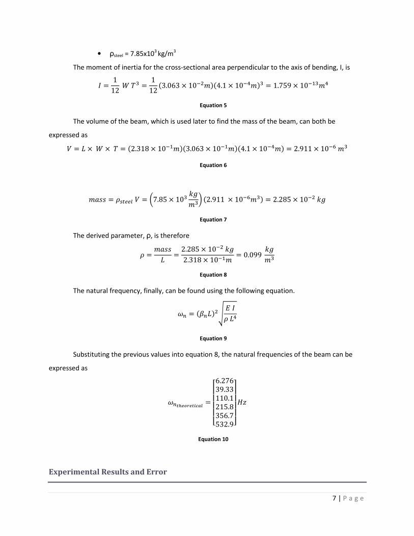
• ρsteel = 7.85x103

kg/m3

The moment of inertia for the cross-sectional area perpendicular to the axis of bending, I, is

� = 112 ) *+ = 112 �3.063 × 10-�.��4.1 × 10-�.�+ = 1.759 × 10-/+.�

Equation 5

The volume of the beam, which is used later to find the mass of the beam, can both be

expressed as

0 = 1 × ) × * = �2.318 × 10-/.��3.063 × 10-/.��4.1 × 10-�.� = 2.911 × 10-2 .+

Equation 6

.(33 = 45667 0 = 87.85 × 10+ 9:.+; �2.911 × 10-2.+� = 2.285 × 10-� 9:

Equation 7

The derived parameter, ρ, is therefore

= .(331 = 2.285 × 10-� 9:2.318 × 10-/. = 0.099 9:.+

Equation 8

The natural frequency, finally, can be found using the following equation.

< = ��<1��= � � 1�

Equation 9

Substituting the previous values into equation 8, the natural frequencies of the beam can be

expressed as

<>?@AB@>CDEF =������6.27639.33110.1215.8356.7532.9$%

%%%& GH

Equation 10

Experimental Results and Error

8 | P a g e

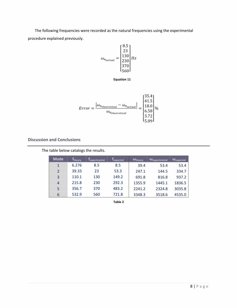
The following frequencies were recorded as the natural frequencies using the experimental

procedure explained previously.

<ED>IEF =������

8.523130230370560$%%%%& GH

Equation 11

�''J' = K<>?@AB@>CDEF − <ED>IEFK<>?@AB@>CDEF=

������35.441.518.06.583.725.09$%

%%%& %

Discussion and Conclusions

The table below catalogs the results.

Mode ftheory fexperimental fexpected ωtheory ωexperimental ωexpected

1 6.276 8.5 8.5 39.4 53.4 53.4

2 39.33 23 53.3 247.1 144.5 334.7

3 110.1 130 149.2 691.8 816.8 937.2

4 215.8 230 292.3 1355.9 1445.1 1836.5

5 356.7 370 483.2 2241.2 2324.8 3035.8

6 532.9 560 721.8 3348.3 3518.6 4535.0

Table 2

9 | P a g e

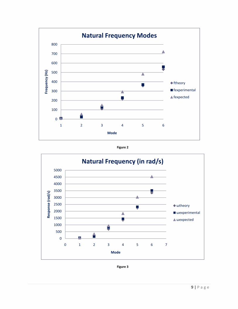
Figure 2

Figure 3

0

100

200

300

400

500

600

700

800

1 2 3 4 5 6

Fre

qu

en

cy (

Hz)

Mode

Natural Frequency Modes

ftheory

fexperimental

fexpected

0

500

1000

1500

2000

2500

3000

3500

4000

4500

5000

0 1 2 3 4 5 6 7

Re

spo

nse

(ra

d/s

)

Mode

Natural Frequency (in rad/s)

ωtheory

ωexperimental

ωexpected

10 | P a g e

References

“Structures Lab 1 – Cantilever Beam Vibration Test.” Handout

MathCAD Work

The length of the beam

L 9.125in 2.31775 101−

× m=:=

W 1.206in 3.0632 102−

× m=:=

T 0.00041m 4.1 104−

× m=:=

Modulus of Elasticity for the beam

E 29.5 106

⋅ psi 2.034 1011

× Pa=:=

Moment of inertia

I1

12W⋅ T

3⋅ 1.759 10

13−× m

4⋅=:=

The density of steel

ρSteel 7.85gm

cm3

7.85 103

×

kg

m3

=:=

The volume of the beam

V L W⋅ T⋅ 2.911 106−

× m3

⋅=:=

The mass of the beam

mass ρSteel V⋅ 2.285 102−

× kg=:=

The parameter, ρ, which is mass per length

ρlengthmass

L0.099

kg

m=:=

11 | P a g e

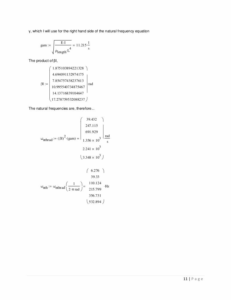
γ, which I wil l use for the right hand side of the natural frequency equation

gamE I⋅

ρlength L4

⋅

11.2151

s=:=

The product of βl,

βl

1.875103894221328

4.694091132974175

7.854757438237613

10.995540734875467

14.13716839104647

17.278759532088237

rad⋅:=

The natural frequencies are, therefore...

ωnthrad βl( )2

gam( )⋅

39.432

247.115

691.929

1.356 103

×

2.241 103

×

3.348 103

×

rad

s⋅=:=

ωnth ωnthrad1

2 π⋅ rad

⋅

6.276

39.33

110.124

215.799

356.731

532.894

Hz⋅=:=

12 | P a g e

ωnexp

8.5

23

130

230

370

560

Hz:=

Errorωnexp ωnth−

ωnth

35.442

41.52−

18.049

6.581

3.72

5.087

%⋅=:=