Chapter 5 Autoregressive Conditional Heteroskedasticity...
22
Chapter 5 Autoregressive Conditional Heteroskedasticity Models 5.1 Modeling Volatility In most econometric models the variance of the disturbance term is assumed to be constant (homoscedasticity). However, there is a number of economics and finance series that exhibit periods of unusual large volatility, followed by periods of relative tranquility. Then, in such cases the assumption of homoscedasticity is not appropri- ate. For example, consider the daily changes in the NYSE International 100 Index, April 5, 2004 - September 20, 2011, shown in Figure 5.1. One easy way to understand volatility is modeling it explicitly, for example in y t +1 = ε t +1 x t (5.1) where y t +1 is the variable of interest, ε t +1 is a white-noise disturbance term with variance σ 2 , and x t is an independent variable that is observed at time t . If x t = x t -1 = x t -2 = ··· = constant, then the {y t } is a familiar white-noise process with a constant variance. However, if they are not constant, the variance of y t +1 conditional on the observable value of x t is var(y t +1 |x t )= x 2 t σ 2 (5.2) If {x t } exhibit positive serial correlation, the conditional variance of the {y t } se- quence will also exhibit positive serial correlation. We can write the model in loga- rithm form and introduce the coefficients a 0 and a 1 to have log(y t )= a 0 + a 1 log(x t -1 )+ e t (5.3) where e t = log(ε t ). 43
Transcript of Chapter 5 Autoregressive Conditional Heteroskedasticity...
Chapter 5
Autoregressive Conditional HeteroskedasticityModels
5.1 Modeling Volatility
In most econometric models the variance of the disturbance term is assumed to be
constant (homoscedasticity). However, there is a number of economics and finance
series that exhibit periods of unusual large volatility, followed by periods of relative
tranquility. Then, in such cases the assumption of homoscedasticity is not appropri-
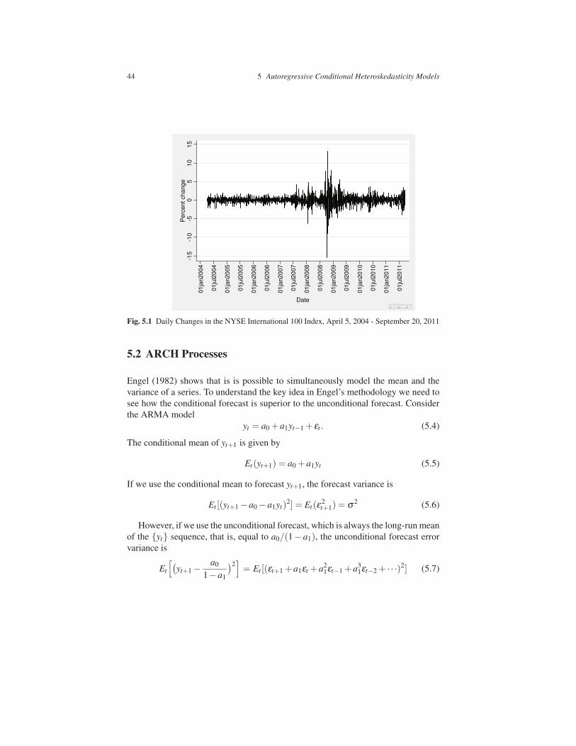
ate. For example, consider the daily changes in the NYSE International 100 Index,
April 5, 2004 - September 20, 2011, shown in Figure 5.1.
One easy way to understand volatility is modeling it explicitly, for example in
yt+1 = εt+1xt (5.1)
where yt+1 is the variable of interest, εt+1 is a white-noise disturbance term with
variance σ2, and xt is an independent variable that is observed at time t.
If xt = xt−1 = xt−2 = · · · = constant, then the {yt} is a familiar white-noise process
with a constant variance. However, if they are not constant, the variance of yt+1
conditional on the observable value of xt is
var(yt+1|xt) = x2t σ2 (5.2)
If {xt} exhibit positive serial correlation, the conditional variance of the {yt} se-
quence will also exhibit positive serial correlation. We can write the model in loga-
rithm form and introduce the coefficients a0 and a1 to have
log(yt) = a0 +a1 log(xt−1)+ et (5.3)
where et = log(εt).
43
44 5 Autoregressive Conditional Heteroskedasticity Models
-15
-10
-50
510
15
Perc
ent change
01ja
n2004
01ju
l2004
01ja
n2005
01ju
l2005
01ja
n2006
01ju
l2006
01ja
n2007
01ju
l2007
01ja
n2008
01ju
l2008
01ja
n2009
01ju
l2009
01ja
n2010
01ju
l2010
01ja
n2011
01ju
l2011
Date
Fig. 5.1 Daily Changes in the NYSE International 100 Index, April 5, 2004 - September 20, 2011
5.2 ARCH Processes
Engel (1982) shows that is is possible to simultaneously model the mean and the
variance of a series. To understand the key idea in Engel’s methodology we need to
see how the conditional forecast is superior to the unconditional forecast. Consider
the ARMA model
yt = a0 +a1yt−1 + εt . (5.4)
The conditional mean of yt+1 is given by
Et(yt+1) = a0 +a1yt (5.5)
If we use the conditional mean to forecast yt+1, the forecast variance is
Et [(yt+1−a0−a1yt)2] = Et(ε
2t+1) = σ2 (5.6)
However, if we use the unconditional forecast, which is always the long-run mean
of the {yt} sequence, that is, equal to a0/(1− a1), the unconditional forecast error
variance is
Et
[
(
yt+1−a0
1−a1
)2]
= Et [(εt+1 +a1εt +a21εt−1 +a3
1εt−2 + · · ·)2] (5.7)

5.2 ARCH Processes 45
=σ2
1−a21
Because 1/(1− a21) > 1, the unconditional forecast has a greater variance than
the conditional forecast. Hence, conditional forecasts are preferable.
In the same way, if the variance of {εt} is not constant, you can estimate any
tendency using an ARMA model. For example, if {ε̂t} are the estimated residuals
of the model yt = a0 +a1yt−1 + εt , the conditional variance of yt+1 is
var(yt+1|yt) = Et [(yt+1−a0−a1yt)2] (5.8)
= Et(εt+1)2
We do not assume that it is constant as in Equation 5.6. Let’s say we can estimate
it using the conditional variance as an AR(q) process using squares of the estimated
residuals
ε̂2t = α0 +α1ε̂2
t−1 +α2ε̂2t−2 + · · ·+αqε̂2
t−q + v (5.9)
where v is a white-noise process. If α1 = α2 = · = αn= 0, the estimated variance
is simply a constant α0 = σ2. Otherwise we can use Equation 5.9 to forecast the
conditional variance at t +1,
Et(ε̂2t+1) = α0 +α1ε̂2
t +α2ε̂2t−1 + · · ·+αqε̂2
t+1−q (5.10)
This is why Equation 5.9 is called an autoregressive conditional heteroscedasticity
ARCH model. The linear specification in 5.9 is actually not the most convenient.
Models for {yt} and the conditional variance can be estimated simultaneously using
maximum likelihood. In most cases v enters in a multiplicative fashion.
Engel (1982) proposed the following multiplicative conditional heteroscedastic-
ity model
εt = vt
√
α0 +α1ε2t−1 (5.11)
where vt is a white-noise process with σ2v = 1, vt and εt−1 are independent of each
other, α0 > 0, and 0≤ α1 ≤ 1.
Consider the properties of εt .
1. The unconditional expectation of εt is zero
E(εt) = E[vt(α0 +α1ε2t−1)
1/2] (5.12)
= E(vt)E[(α0 +α1ε2t−1)
1/2] = 0
2. Because E(vtvt−1),
E(εtεt−1) = 0 i 6= 0 (5.13)
46 5 Autoregressive Conditional Heteroskedasticity Models
3. The unconditional variance of εt is
E(ε2t ) = E[v2
t (α0 +α1ε2t−1)] (5.14)
= E(v2t )E(α0 +α1ε2
t−1)
because σ2v = 1 and the unconditional variance of εt is equal to the unconditional
variance of εt−1, hence
E(ε2t ) =
α0
1−α1(5.15)
4. The conditional mean of εt is zero
E(εt |εt−1,εt−2, . . .) = Et−1(vt)Et−1(α0 +α1ε2t−1)
1/2 = 0 (5.16)
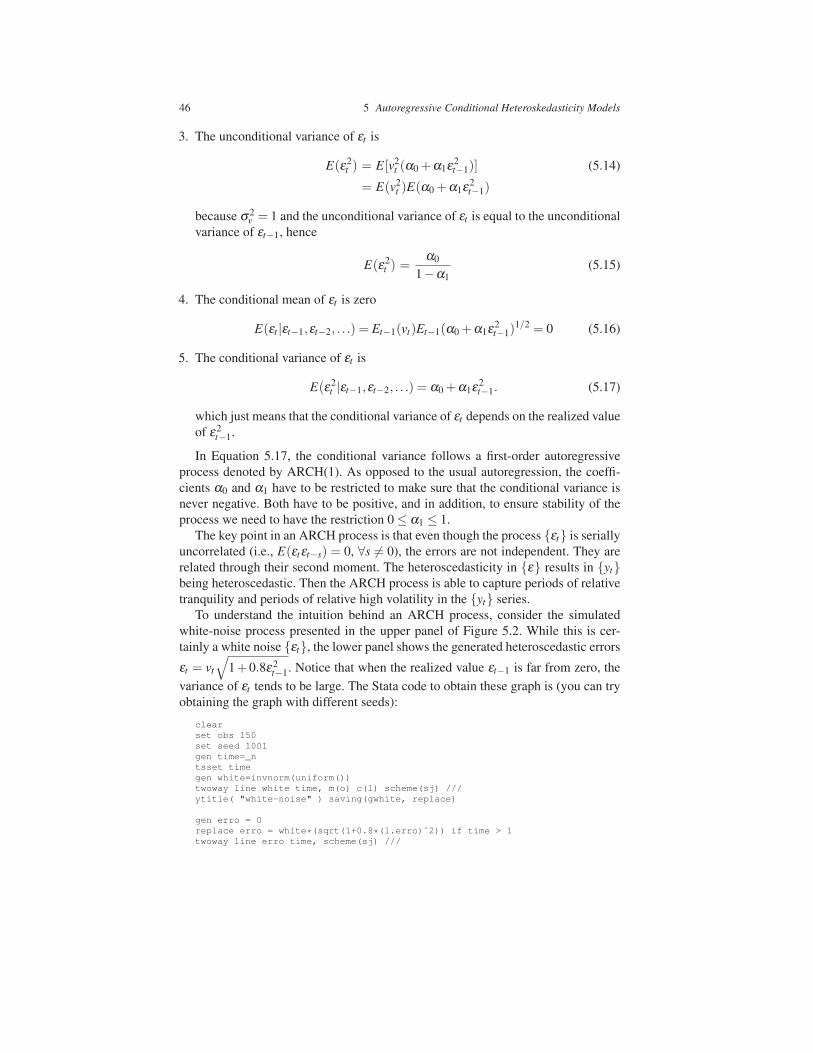
5. The conditional variance of εt is
E(ε2t |εt−1,εt−2, . . .) = α0 +α1ε2
t−1. (5.17)
which just means that the conditional variance of εt depends on the realized value
of ε2t−1.
In Equation 5.17, the conditional variance follows a first-order autoregressive
process denoted by ARCH(1). As opposed to the usual autoregression, the coeffi-
cients α0 and α1 have to be restricted to make sure that the conditional variance is
never negative. Both have to be positive, and in addition, to ensure stability of the
process we need to have the restriction 0≤ α1 ≤ 1.
The key point in an ARCH process is that even though the process {εt} is serially
uncorrelated (i.e., E(εtεt−s) = 0, ∀s 6= 0), the errors are not independent. They are
related through their second moment. The heteroscedasticity in {ε} results in {yt}being heteroscedastic. Then the ARCH process is able to capture periods of relative
tranquility and periods of relative high volatility in the {yt} series.
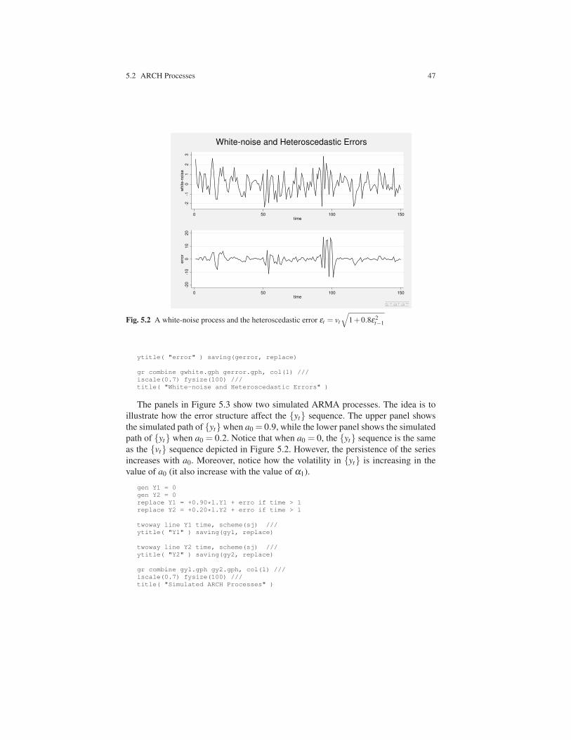
To understand the intuition behind an ARCH process, consider the simulated
white-noise process presented in the upper panel of Figure 5.2. While this is cer-
tainly a white noise {εt}, the lower panel shows the generated heteroscedastic errors
εt = vt
√
1+0.8ε2t−1. Notice that when the realized value εt−1 is far from zero, the
variance of εt tends to be large. The Stata code to obtain these graph is (you can try
obtaining the graph with different seeds):
clear
set obs 150
set seed 1001
gen time=_n
tsset time
gen white=invnorm(uniform())
twoway line white time, m(o) c(l) scheme(sj) ///
ytitle( "white-noise" ) saving(gwhite, replace)
gen erro = 0
replace erro = white*(sqrt(1+0.8*(l.erro)ˆ2)) if time > 1
twoway line erro time, scheme(sj) ///
5.2 ARCH Processes 47
-2-1
01
23
white-n
ois
e
0 50 100 150
time
-20
-10
010
20
err
or
0 50 100 150
time
White-noise and Heteroscedastic Errors
Fig. 5.2 A white-noise process and the heteroscedastic error εt = vt
√
1+0.8ε2t−1
ytitle( "error" ) saving(gerror, replace)
gr combine gwhite.gph gerror.gph, col(1) ///
iscale(0.7) fysize(100) ///
title( "White-noise and Heteroscedastic Errors" )
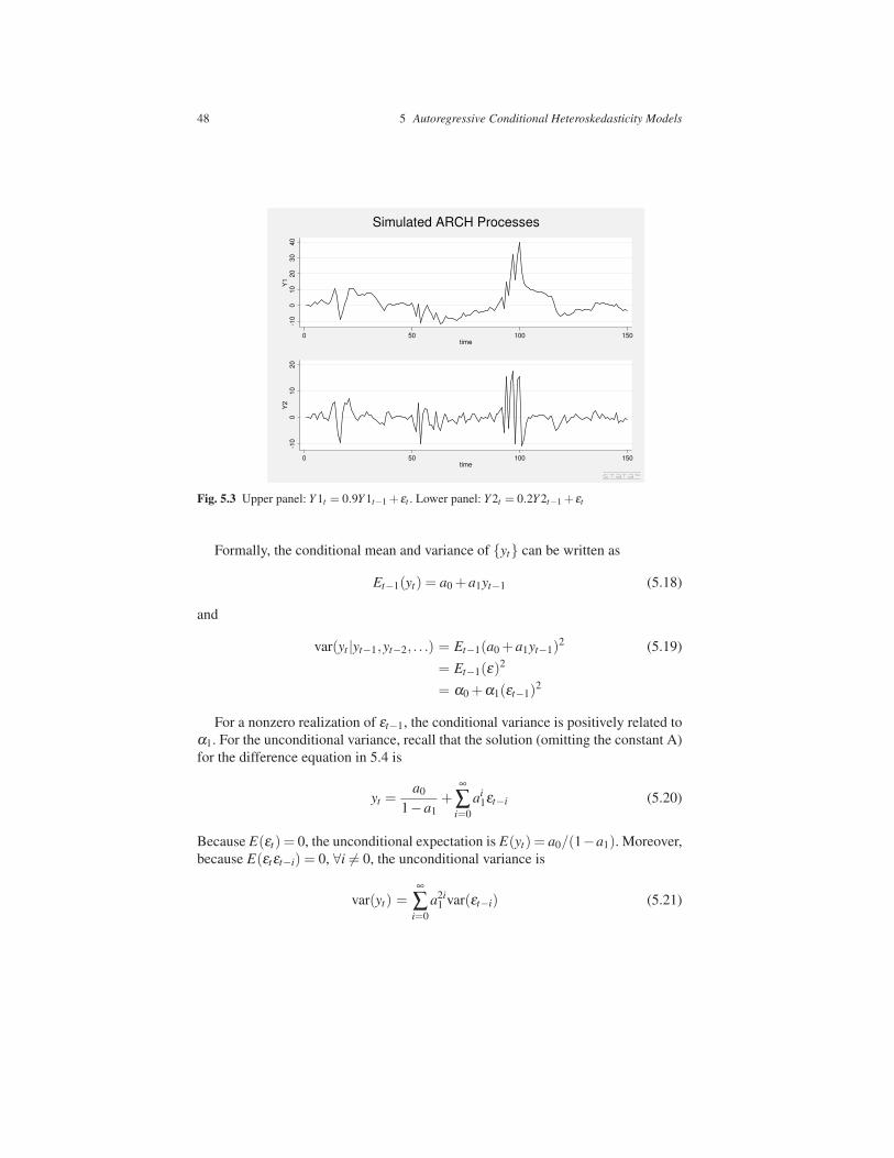
The panels in Figure 5.3 show two simulated ARMA processes. The idea is to
illustrate how the error structure affect the {yt} sequence. The upper panel shows
the simulated path of {yt}when a0 = 0.9, while the lower panel shows the simulated
path of {yt} when a0 = 0.2. Notice that when a0 = 0, the {yt} sequence is the same
as the {vt} sequence depicted in Figure 5.2. However, the persistence of the series
increases with a0. Moreover, notice how the volatility in {yt} is increasing in the
value of a0 (it also increase with the value of α1).
gen Y1 = 0
gen Y2 = 0
replace Y1 = +0.90*l.Y1 + erro if time > 1
replace Y2 = +0.20*l.Y2 + erro if time > 1
twoway line Y1 time, scheme(sj) ///
ytitle( "Y1" ) saving(gy1, replace)
twoway line Y2 time, scheme(sj) ///
ytitle( "Y2" ) saving(gy2, replace)
gr combine gy1.gph gy2.gph, col(1) ///
iscale(0.7) fysize(100) ///
title( "Simulated ARCH Processes" )
48 5 Autoregressive Conditional Heteroskedasticity Models
-10
010
20
30
40
Y1
0 50 100 150
time
-10
010
20
Y2
0 50 100 150
time
Simulated ARCH Processes
Fig. 5.3 Upper panel: Y 1t = 0.9Y 1t−1 + εt . Lower panel: Y 2t = 0.2Y 2t−1 + εt
Formally, the conditional mean and variance of {yt} can be written as
Et−1(yt) = a0 +a1yt−1 (5.18)
and
var(yt |yt−1,yt−2, . . .) = Et−1(a0 +a1yt−1)2 (5.19)
= Et−1(ε)2
= α0 +α1(εt−1)2
For a nonzero realization of εt−1, the conditional variance is positively related to
α1. For the unconditional variance, recall that the solution (omitting the constant A)
for the difference equation in 5.4 is
yt =a0
1−a1+
∞
∑i=0
ai1εt−i (5.20)
Because E(εt) = 0, the unconditional expectation is E(yt) = a0/(1−a1). Moreover,
because E(εtεt−i) = 0, ∀i 6= 0, the unconditional variance is
var(yt) =∞
∑i=0
a2i1 var(εt−i) (5.21)
5.3 GARCH Processes 49
=( α0
1−α1
)( 1
1−a21
)
where the last equality follows from the result in Equation 5.15. It is easy to see that
the unconditional variance in also increasing in α1 (and in the absolute value of a1).
The ARCH process presented in Equation 5.11 can be extended in a number of
ways. The most straight forward is considering the higher-order ARCH(q) process
εt = vt
√
α0 +q
∑i=1
αiε2t−i (5.22)
5.3 GARCH Processes
The ARCH idea was extended in Bollerslev (1986) to allow an ARMA process
embedded in the conditional variance. Let the error process be
εt = vt
√
ht (5.23)
where σ2 = 1, and
ht = α0 +q
∑i=1
αiε2t−1 +
p
∑i=1
βiht−1 (5.24)
The conditional and unconditional means of εt are both zero because {vt} is a
white-noise process. The key point is that the conditional variance of εt is given
by Et−1(ε2t ) = ht , which is the ARMA process given in Equation 5.24.
This heteroscedastic variance that allows autoregressive and moving average
components is called GARCH(p,q), where the G in GARCH denotes generalized.
Notice that a GARCH(0,1) is just the ARCH model in Equation 5.11. The impor-
tant restriction in a GARCH process is that all coefficients in Equation 5.24 must be
positive and must ensure that the variance is finite (i.e., its characteristic roots must
lie inside the unit circle).
A simple procedure to know if a series {yt} follows a GARCH process is to
estimate the best fitting ARMA process and then obtain the fitted errors {ε̂t} and the
squares of the fitted errors {ε̂2t }. White the ACF and the PACF of the fitted errors
should be consistent with a white noise, the squared fitted errors should indicate that
they follow an ARMA process. It is also useful that besides the ACF and PACF, we
use the Ljung-Box Q-statistic.Let’s follow the previous suggested steps in Stata for the previously generated
process Y 1, under the assumption that we know that it follows an ARMA(1,0) pro-cess with no constant (otherwise we need to search for the optimal ARMA(p,q)).
arima Y1, arima(1,0,0) nocons
predict eserro, res
gen eserro2 = eserroˆ2
corrgram eserro2, lags(20)
-1 0 1 -1 0 1
LAG AC PAC Q Prob>Q [Autocorrelation] [Partial Autocor]
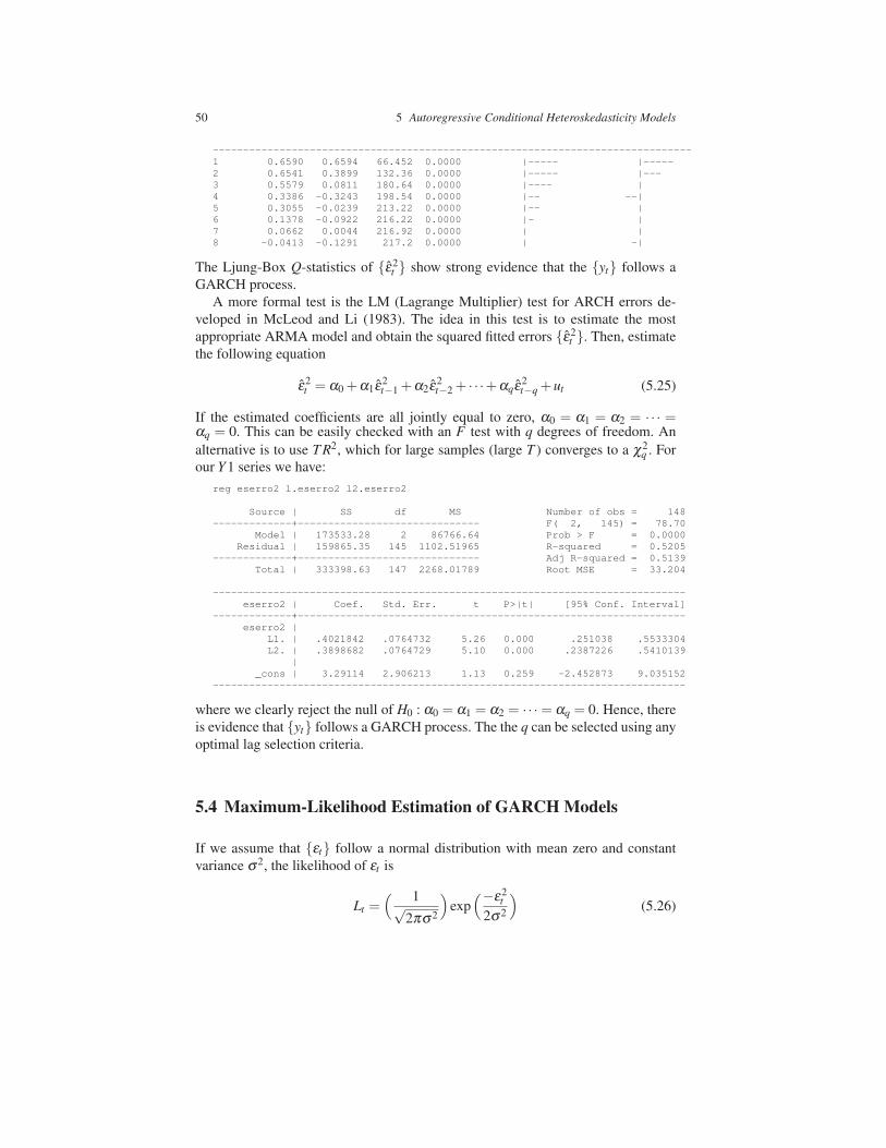
50 5 Autoregressive Conditional Heteroskedasticity Models
-------------------------------------------------------------------------------
1 0.6590 0.6594 66.452 0.0000 |----- |-----
2 0.6541 0.3899 132.36 0.0000 |----- |---
3 0.5579 0.0811 180.64 0.0000 |---- |
4 0.3386 -0.3243 198.54 0.0000 |-- --|
5 0.3055 -0.0239 213.22 0.0000 |-- |
6 0.1378 -0.0922 216.22 0.0000 |- |
7 0.0662 0.0044 216.92 0.0000 | |
8 -0.0413 -0.1291 217.2 0.0000 | -|
The Ljung-Box Q-statistics of {ε̂2t } show strong evidence that the {yt} follows a
GARCH process.
A more formal test is the LM (Lagrange Multiplier) test for ARCH errors de-
veloped in McLeod and Li (1983). The idea in this test is to estimate the most
appropriate ARMA model and obtain the squared fitted errors {ε̂2t }. Then, estimate
the following equation
ε̂2t = α0 +α1ε̂2
t−1 +α2ε̂2t−2 + · · ·+αqε̂2
t−q +ut (5.25)
If the estimated coefficients are all jointly equal to zero, α0 = α1 = α2 = · · · =αq = 0. This can be easily checked with an F test with q degrees of freedom. An
alternative is to use T R2, which for large samples (large T ) converges to a χ2q . For
our Y 1 series we have:
reg eserro2 l.eserro2 l2.eserro2
Source | SS df MS Number of obs = 148
-------------+------------------------------ F( 2, 145) = 78.70
Model | 173533.28 2 86766.64 Prob > F = 0.0000
Residual | 159865.35 145 1102.51965 R-squared = 0.5205
-------------+------------------------------ Adj R-squared = 0.5139
Total | 333398.63 147 2268.01789 Root MSE = 33.204
------------------------------------------------------------------------------
eserro2 | Coef. Std. Err. t P>|t| [95% Conf. Interval]
-------------+----------------------------------------------------------------
eserro2 |
L1. | .4021842 .0764732 5.26 0.000 .251038 .5533304
L2. | .3898682 .0764729 5.10 0.000 .2387226 .5410139
|
_cons | 3.29114 2.906213 1.13 0.259 -2.452873 9.035152
------------------------------------------------------------------------------
where we clearly reject the null of H0 : α0 = α1 = α2 = · · ·= αq = 0. Hence, there
is evidence that {yt} follows a GARCH process. The the q can be selected using any
optimal lag selection criteria.
5.4 Maximum-Likelihood Estimation of GARCH Models
If we assume that {εt} follow a normal distribution with mean zero and constant
variance σ2, the likelihood of εt is
Lt =( 1√
2πσ2
)
exp(−ε2
t
2σ2
)
(5.26)
5.4 Maximum-Likelihood Estimation of GARCH Models 51
Because {εt} are independent, the likelihood function of the of the joint realizations
of ε1,ε2, . . . ,εT is
L =T
∏t=1
( 1√2πσ2
)
exp(−ε2
t
2σ2
)
. (5.27)
Taking the logs we obtain the log-likelihood function
logL =−T
2log(2π)− T
2logσ2− 1
2σ2
T
∑t=1
(εt)2 (5.28)
If we want to estimate the simple model yt = βxt + εt , the maximum log-likelihood
function becomes
logL =−T
2log(2π)− T
2logσ2− 1
2σ2
T
∑t=1
(yt −βxt)2. (5.29)
Then, the maximum likelihood estimates of β and σ2 can be obtained from the
following first-oder conditions
∂ logL
∂σ2= − T
2σ2+
1
2σ4
T
∑t=1
(yt +βxt)2 = 0 (5.30)
∂ logL
∂β=
1
σ2
T
∑t=1
(ytxt +βx2t ) = 0 (5.31)
which yield the familiar OLS results σ̂2 = ∑ε2t /T and β̂ = ∑xtyt/∑x2
t . A close
form solution is possible because the FOC are linear.
How do we introduce heteroscedastic errors in this familiar maximum likelihood
procedure? Let’s assume that yt follows an ARCH(1) process. Hence, εt is
εt = vt
√
ht (5.32)
where the conditional variance of εt is ht . Then the likelihood function becomes
L =T
∏t=1
( 1√2πht
)
exp(−ε2
t
2ht
)
(5.33)
and the log-likelihood function is
logL =−T
2log(2π)− 1
2
T
∑t=1
loght −1
2
2
∑t=1
(ε2t /ht). (5.34)
With εt = yt −βxt and ht = α0 +α1ε2t−1 we have
logL = −T −1
2log(2π)− 1
2
T
∑t=2
log(α0 +α1ε2t−1) (5.35)
52 5 Autoregressive Conditional Heteroskedasticity Models
−1
2
2
∑t=2
[(yt −βxt)2/(α0 +α1ε2
t−1)]
= −T −1
2log(2π)− 1
2
T
∑t=2
log(α0 +α1(yt−1−βxt−1)2)
−1
2
2
∑t=2
[(yt −βxt)2/(α0 +α1(yt−1−βxt−1)
2)],
where the first observation is lost because of the lag. While the FOC yield compli-
cated nonlinear equations that do not have a close-form solution, this log-likelihood
function can be maximized using numerical methods.
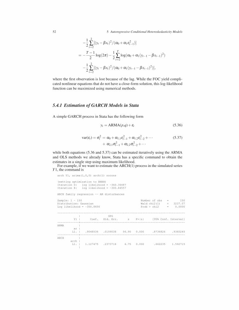
5.4.1 Estimation of GARCH Models in Stata
A simple GARCH process in Stata has the following form
yt = ARMA(p,q)+ εt (5.36)
var(εt ) = σ2t = α0 +α1,1ε2
t−1 +α1,2ε2t−2 + · · · (5.37)
+ α2,1σ2t−1 +α2,2σ2
t−2 + · · ·
while both equations (5.36 and 5.37) can be estimated iteratively using the ARMA
and OLS methods we already know, Stata has a specific command to obtain the
estimates in a single step using maximum likelihood.For example, if we want to estimate the ARCH(1) process in the simulated series
Y 1, the command is
arch Y1, arima(1,0,0) arch(1) nocons
(setting optimization to BHHH)
Iteration 0: log likelihood = -360.36487
Iteration 8: log likelihood = -300.84557
ARCH family regression -- AR disturbances
Sample: 1 - 150 Number of obs = 150
Distribution: Gaussian Wald chi2(1) = 3237.07
Log likelihood = -300.8456 Prob > chi2 = 0.0000
------------------------------------------------------------------------------
| OPG
Y1 | Coef. Std. Err. z P>|z| [95% Conf. Interval]
-------------+----------------------------------------------------------------
ARMA |
ar |
L1. | .9048536 .0159038 56.90 0.000 .8736826 .9360245
-------------+----------------------------------------------------------------
ARCH |
arch |
L1. | 1.127475 .2373718 4.75 0.000 .662235 1.592715
|
5.4 Maximum-Likelihood Estimation of GARCH Models 53
_cons | .6363727 .1757892 3.62 0.000 .2918322 .9809133
------------------------------------------------------------------------------
That can be written as
Y 1t = 0.90Y 1t−1 + εt (5.38)
σ2t = 0.64+1.13ε2
t−1 (5.39)
For an AR(1) with GARCH(1,1) we need
arch Y1, arima(1,0,0) arch(1) garch(1) nocons
(output omitted)
which yields
Y 1t = 0.90Y 1t−1 + εt (5.40)
σ2t = 0.65+1.13ε2
t−1−0.03σ2t−1. (5.41)
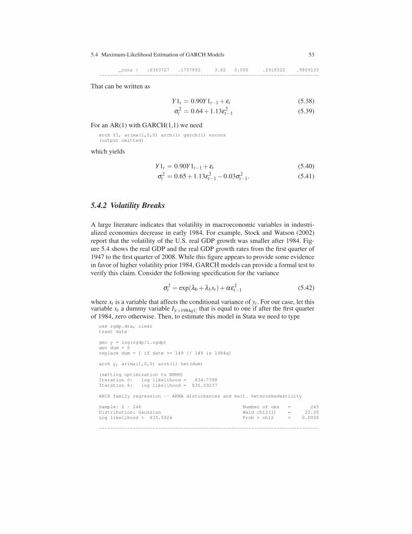
5.4.2 Volatility Breaks
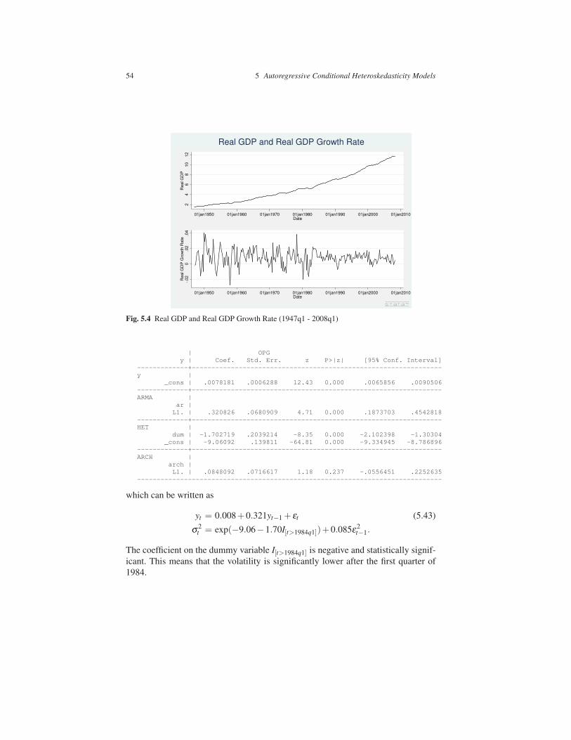
A large literature indicates that volatility in macroeconomic variables in industri-
alized economies decrease in early 1984. For example, Stock and Watson (2002)
report that the volatility of the U.S. real GDP growth was smaller after 1984. Fig-
ure 5.4 shows the real GDP and the real GDP growth rates from the first quarter of
1947 to the first quarter of 2008. While this figure appears to provide some evidence
in favor of higher volatility prior 1984, GARCH models can provide a formal test to
verify this claim. Consider the following specification for the variance
σ2t = exp(λ0 +λ1xt)+αε2
t−1 (5.42)
where xt is a variable that affects the conditional variance of yt . For our case, let thisvariable xt a dummy variable I[t>1984q1] that is equal to one if after the first quarter
of 1984, zero otherwise. Then, to estimate this model in Stata we need to type
use rgdp.dta, clear
tsset date
gen y = log(rgdp/l.rgdp)
gen dum = 0
replace dum = 1 if date >= 149 // 149 is 1984q1
arch y, arima(1,0,0) arch(1) het(dum)
(setting optimization to BHHH)
Iteration 0: log likelihood = 834.7398
Iteration 6: log likelihood = 835.59237
ARCH family regression -- ARMA disturbances and mult. heteroskedasticity
Sample: 2 - 246 Number of obs = 245
Distribution: Gaussian Wald chi2(1) = 22.20
Log likelihood = 835.5924 Prob > chi2 = 0.0000
------------------------------------------------------------------------------
54 5 Autoregressive Conditional Heteroskedasticity Models
24
68
10
12
Real G
DP
01jan1950 01jan1960 01jan1970 01jan1980 01jan1990 01jan2000 01jan2010Date
-.02
0.0
2.0
4R
eal G
DP
Gro
wth
Rate
01jan1950 01jan1960 01jan1970 01jan1980 01jan1990 01jan2000 01jan2010Date
Real GDP and Real GDP Growth Rate
Fig. 5.4 Real GDP and Real GDP Growth Rate (1947q1 - 2008q1)
| OPG
y | Coef. Std. Err. z P>|z| [95% Conf. Interval]
-------------+----------------------------------------------------------------
y |
_cons | .0078181 .0006288 12.43 0.000 .0065856 .0090506
-------------+----------------------------------------------------------------
ARMA |
ar |
L1. | .320826 .0680909 4.71 0.000 .1873703 .4542818
-------------+----------------------------------------------------------------
HET |
dum | -1.702719 .2039214 -8.35 0.000 -2.102398 -1.30304
_cons | -9.06092 .139811 -64.81 0.000 -9.334945 -8.786896
-------------+----------------------------------------------------------------
ARCH |
arch |
L1. | .0848092 .0716617 1.18 0.237 -.0556451 .2252635
------------------------------------------------------------------------------
which can be written as
yt = 0.008+0.321yt−1 + εt (5.43)
σ2t = exp(−9.06−1.70I[t>1984q1])+0.085ε2
t−1.
The coefficient on the dummy variable I[t>1984q1] is negative and statistically signif-
icant. This means that the volatility is significantly lower after the first quarter of
1984.
5.5 ARCH-in-mean Models 55
5.5 ARCH-in-mean Models
The ARCH-in-mean (ARCH-M) models were introduced by Engel, Lilien, and
Robins (1987). The idea is to allow for the mean of a sequence to depend on its
conditional variance. If the riskiness of an asset can be measured by the variance
of its returns, the risk premium will be an increasing function of the conditional
variance of returns. This can be formally modeled with ARCH-M models.
Engel, Lilien, and Robins (1987) write the excess return of holding a risky asset
as
yt = µt + εt (5.44)
where yt is the excess return from holding a long-term asset relative to a one-period
treasury bill, µt is the risk premium necessary to induce the risk-averse agent to hold
the long-term asset rather than the one-period bond, and εt is the unforecastable
shock to the excess return on the long-term asset.
The expected excess return from holding the long-term asset is equal to the risk
premium
Et−1(yt) = µt . (5.45)
We can model the risk premium as a function of the conditional variance of ε . Let ht
be the conditional variance of εt . Then the risk premium can be modeled to depend
on the conditional variance
µt = β +δht , δ > 0 (5.46)
and where the conditional variance ht follows an ARCH(q) process
ht = α0 +q
∑i=1
αiε2t−i (5.47)
Hence, the ARCH-M model is the combination of Equations 5.44, 5.46, and 5.47.
If α1 = α2 = · · · = αq = 0, the ARCH-M models becomes the traditional constant
risk premium model.
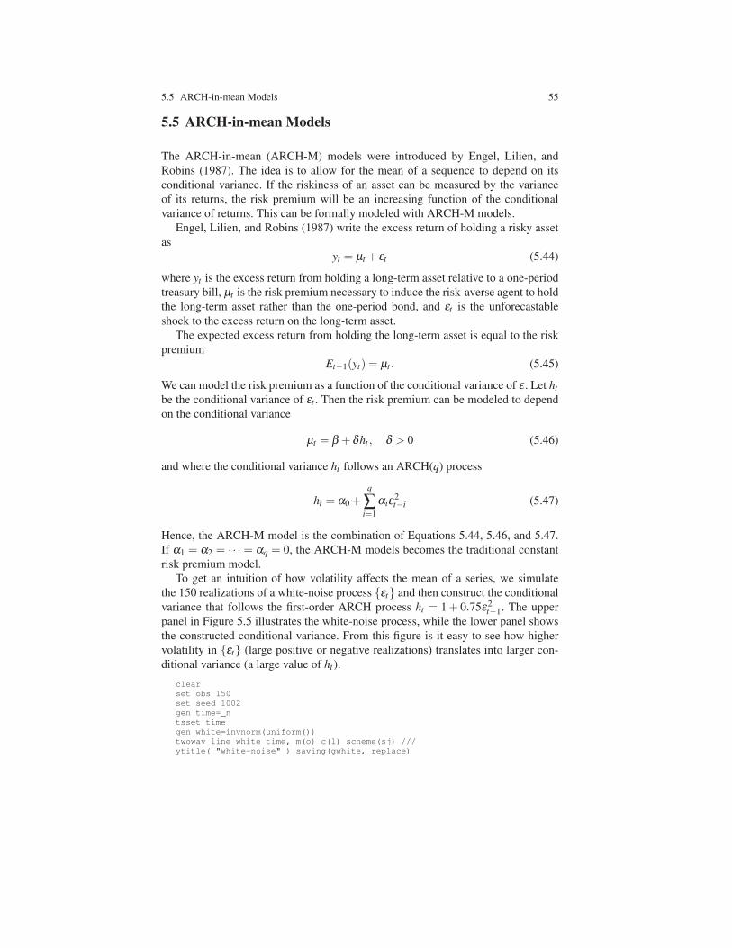
To get an intuition of how volatility affects the mean of a series, we simulate
the 150 realizations of a white-noise process {εt} and then construct the conditional
variance that follows the first-order ARCH process ht = 1+ 0.75ε2t−1. The upper
panel in Figure 5.5 illustrates the white-noise process, while the lower panel shows
the constructed conditional variance. From this figure is it easy to see how higher
volatility in {εt} (large positive or negative realizations) translates into larger con-
ditional variance (a large value of ht ).
clear
set obs 150
set seed 1002
gen time=_n
tsset time
gen white=invnorm(uniform())
twoway line white time, m(o) c(l) scheme(sj) ///
ytitle( "white-noise" ) saving(gwhite, replace)
56 5 Autoregressive Conditional Heteroskedasticity Models
-4-2
02
4
white-n
ois
e
0 50 100 150
time
05
10
15
conditio
nal variance
0 50 100 150
time
White-noise and Conditional Variance
Fig. 5.5 A white-noise process and conditional variance ht = 1+0.65ε2t−1.
gen vari = 0
replace vari = 1 + 0.75*(l.white)ˆ2 if time > 1
twoway line vari time, scheme(sj) ///
ytitle( "conditional variance" ) saving(gvari, replace)
gr combine gwhite.gph gvari.gph, col(1) ///
iscale(0.7) fysize(100) ///
title( "White-noise and Conditional Variance" )
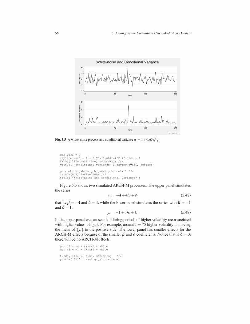
Figure 5.5 shows two simulated ARCH-M processes. The upper panel simulates
the series
yt =−4+4ht + εt (5.48)
that is, β = −4 and δ = 4, while the lower panel simulates the series with β = −1
and δ = 1,
yt =−1+1ht + εt . (5.49)
In the upper panel we can see that during periods of higher volatility are associated
with higher values of {yt}. For example, around t = 75 higher volatility is moving
the mean of {yt} to the positive side. The lower panel has smaller effects for the
ARCH-M effects because of the smaller β and δ coefficients. Notice that if δ = 0,
there will be no ARCH-M effects.
gen Y1 = -4 + 4*vari + white
gen Y2 = -1 + 1*vari + white
twoway line Y1 time, scheme(sj) ///
ytitle( "Y1" ) saving(gy1, replace)
5.5 ARCH-in-mean Models 57
-10
010
20
30
40
Y1
0 50 100 150
time
-50
510
Y2
0 50 100 150
time
Simulated ARCH-M Processes
Fig. 5.6 Upper panel: Y 1t =−4+4ht + εt . Lower panel: Y 2t =−1+1ht + εt .
twoway line Y2 time, scheme(sj) ///
ytitle( "Y2" ) saving(gy2, replace)
gr combine gy1.gph gy2.gph, col(1) ///
iscale(0.7) fysize(100) ///
title( "Simulated ARCH-M Processes" )
The LM test we described before to test for the presence of an ARCH process can
also be used here. However, this test will not help in knowing whether the ARCH
process is an ARCH-M.
The Stata estimation of an ARCH-M process is straight forward. The process for
yt can be extended from Equation 5.36 to include the ARCH-M component
yt = ARMA(p,q)+p
∑i=1
φig(σ2t−i)+ ε (5.50)
and the conditional variance can follow the same form as before
var(εt ) = σ2t = α0 +α1,1ε2
t−1 +α1,2ε2t−2 + · · · (5.51)
+ α2,1σ2t−1 +α2,2σ2
t−2 + · · ·
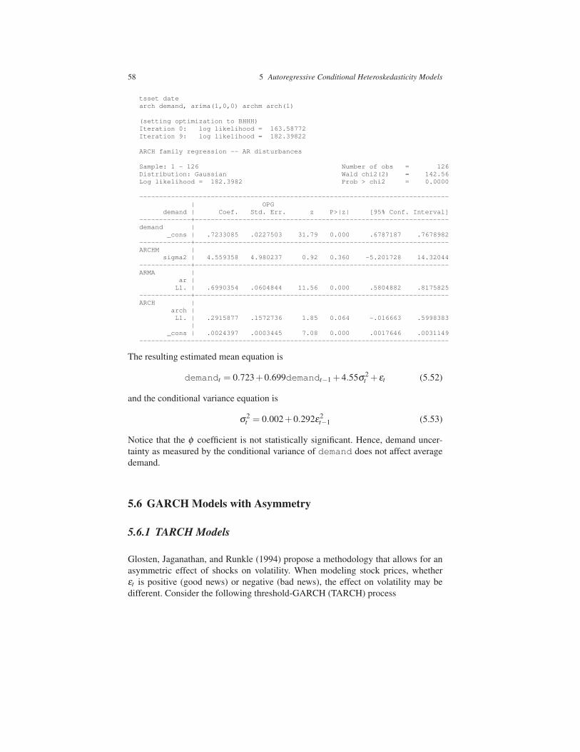
Consider the following example that tests whether demand uncertainty affectsmean demand realizations
use airlines.dta, clear
58 5 Autoregressive Conditional Heteroskedasticity Models
tsset date
arch demand, arima(1,0,0) archm arch(1)
(setting optimization to BHHH)
Iteration 0: log likelihood = 163.58772
Iteration 9: log likelihood = 182.39822
ARCH family regression -- AR disturbances
Sample: 1 - 126 Number of obs = 126
Distribution: Gaussian Wald chi2(2) = 142.56
Log likelihood = 182.3982 Prob > chi2 = 0.0000
------------------------------------------------------------------------------
| OPG
demand | Coef. Std. Err. z P>|z| [95% Conf. Interval]
-------------+----------------------------------------------------------------
demand |
_cons | .7233085 .0227503 31.79 0.000 .6787187 .7678982
-------------+----------------------------------------------------------------
ARCHM |
sigma2 | 4.559358 4.980237 0.92 0.360 -5.201728 14.32044
-------------+----------------------------------------------------------------
ARMA |
ar |
L1. | .6990354 .0604844 11.56 0.000 .5804882 .8175825
-------------+----------------------------------------------------------------
ARCH |
arch |
L1. | .2915877 .1572736 1.85 0.064 -.016663 .5998383
|
_cons | .0024397 .0003445 7.08 0.000 .0017646 .0031149
------------------------------------------------------------------------------
The resulting estimated mean equation is
demandt = 0.723+0.699demandt−1 +4.55σ2t + εt (5.52)
and the conditional variance equation is
σ2t = 0.002+0.292ε2
t−1 (5.53)
Notice that the φ coefficient is not statistically significant. Hence, demand uncer-
tainty as measured by the conditional variance of demand does not affect average
demand.
5.6 GARCH Models with Asymmetry
5.6.1 TARCH Models
Glosten, Jaganathan, and Runkle (1994) propose a methodology that allows for an
asymmetric effect of shocks on volatility. When modeling stock prices, whether
εt is positive (good news) or negative (bad news), the effect on volatility may be
different. Consider the following threshold-GARCH (TARCH) process
5.6 GARCH Models with Asymmetry 59
ht = α0 +α1ε2t−1 +λ1dt−1ε2
t−1 +β1ht−1 (5.54)
where dt−1 is a dummy variable that is equal to one if εt−1 < 0 and it is equal to
zero otherwise.
The intuition in this model is simple. If εt−1 < 0, then dt−1 = 1 and the effect of
the εt−1 shock on volatility ht is given by (α1 +λ1)ε2t−1. On the other hand, if the
shock is positive, then εt−1 ≥ 0 and dt−1 = 0, and the effect of the εt−1 shock on
volatility ht is α1ε2t−1. Hence, if λ1 > 0, negative shocks will have a larger effect on
volatility than positive shocks. The statistical significance of the λ1 coefficient will
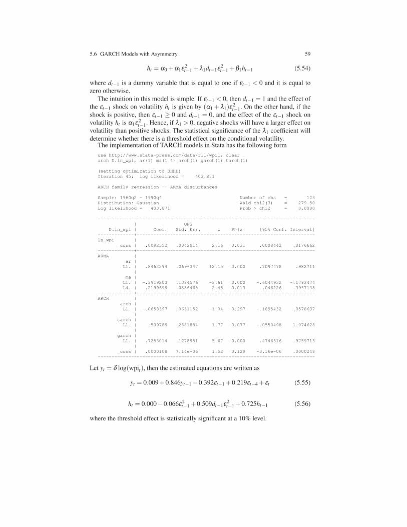
determine whether there is a threshold effect on the conditional volatility.The implementation of TARCH models in Stata has the following form
use http://www.stata-press.com/data/r11/wpi1, clear
arch D.ln_wpi, ar(1) ma(1 4) arch(1) garch(1) tarch(1)
(setting optimization to BHHH)
Iteration 45: log likelihood = 403.871
ARCH family regression -- ARMA disturbances
Sample: 1960q2 - 1990q4 Number of obs = 123
Distribution: Gaussian Wald chi2(3) = 279.50
Log likelihood = 403.871 Prob > chi2 = 0.0000
------------------------------------------------------------------------------
| OPG
D.ln_wpi | Coef. Std. Err. z P>|z| [95% Conf. Interval]
-------------+----------------------------------------------------------------
ln_wpi |
_cons | .0092552 .0042914 2.16 0.031 .0008442 .0176662
-------------+----------------------------------------------------------------
ARMA |
ar |
L1. | .8462294 .0696347 12.15 0.000 .7097478 .982711
|
ma |
L1. | -.3919203 .1084576 -3.61 0.000 -.6044932 -.1793474
L4. | .2199699 .0886465 2.48 0.013 .046226 .3937138
-------------+----------------------------------------------------------------
ARCH |
arch |
L1. | -.0658397 .0631152 -1.04 0.297 -.1895432 .0578637
|
tarch |
L1. | .509789 .2881884 1.77 0.077 -.0550498 1.074628
|
garch |
L1. | .7253014 .1278951 5.67 0.000 .4746316 .9759713
|
_cons | .0000108 7.14e-06 1.52 0.129 -3.16e-06 .0000248
------------------------------------------------------------------------------
Let yt = δ log(wpit), then the estimated equations are written as
yt = 0.009+0.846yt−1−0.392εt−1 +0.219εt−4 + εt (5.55)
ht = 0.000−0.066ε2t−1 +0.509dt−1ε2
t−1 +0.725ht−1 (5.56)
where the threshold effect is statistically significant at a 10% level.
60 5 Autoregressive Conditional Heteroskedasticity Models
5.6.2 EGARCH Models
A second model that allows for asymmetries in the effect of εt is the exponential-
GARCH (EGARCH) model, as proposed in Nelson (1991). One constraint with the
regular GARCH model is that it requires that all estimated coefficients are positive.
The EGARCH specify the conditional variance in the following way
log(ht) = α0 +α1(εt−1/√
ht−1)+λ1|εt−1/√
ht−1|+β1 log(ht−1). (5.57)
There are three features about this specification:
1. Because of the log(ht) form, the implied value of ht can never be negative (re-
gardless of the values of the coefficients).
2. Instead of using εt−1, EGARCH uses a standardized value εt−1/√
ht−1 (which is
a unit free measure).
3. EGARCH allows for leverage effects. If εt−1/√
ht−1 > 0, the effect of the shock
on the log of the conditional variance is α1 +λ1. If εt−1/√
ht−1 < 0, the effect is
−α1 +λ1.
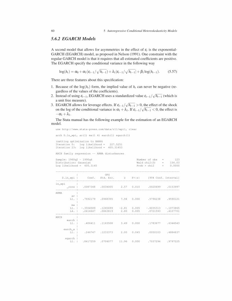
The Stata manual has the following example for the estimation of an EGARCHmodel.
use http://www.stata-press.com/data/r11/wpi1, clear
arch D.ln_wpi, ar(1) ma(1 4) earch(1) egarch(1)
(setting optimization to BHHH)
Iteration 0: log likelihood = 227.5251
Iteration 23: log likelihood = 405.31453
ARCH family regression -- ARMA disturbances
Sample: 1960q2 - 1990q4 Number of obs = 123
Distribution: Gaussian Wald chi2(3) = 156.03
Log likelihood = 405.3145 Prob > chi2 = 0.0000
------------------------------------------------------------------------------
| OPG
D.ln_wpi | Coef. Std. Err. z P>|z| [95% Conf. Interval]
-------------+----------------------------------------------------------------
ln_wpi |
_cons | .0087348 .0034005 2.57 0.010 .0020699 .0153997
-------------+----------------------------------------------------------------
ARMA |
ar |
L1. | .7692179 .0968355 7.94 0.000 .5794238 .9590121
|
ma |
L1. | -.3554589 .1265699 -2.81 0.005 -.6035313 -.1073865
L4. | .2414647 .0863819 2.80 0.005 .0721593 .4107701
-------------+----------------------------------------------------------------
ARCH |
earch |
L1. | .406411 .1163508 3.49 0.000 .1783677 .6344543
|
earch_a |
L1. | .246747 .1233373 2.00 0.045 .0050103 .4884837
|
egarch |
L1. | .8417259 .0704077 11.96 0.000 .7037294 .9797225
5.7 Multivariate GARCH Models 61
|
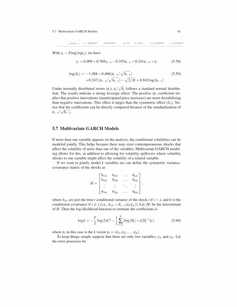
_cons | -1.488427 .6604365 -2.25 0.024 -2.782859 -.1939957
------------------------------------------------------------------------------
With yt = δ log(wpit), we have
yt = 0.009+0.769yt−1−0.355εt−1 +0.241εt−4 + εt (5.58)
log(ht) = −1.488+0.406(εt−1/√
ht−1) (5.59)
+0.247|(εt−1/√
ht−1)−√
2/π|+0.842log(ht−1)
Under normally distributed errors (εt ), εt/√
ht follows a standard normal distribu-
tion. The results indicate a strong leverage effect. The positive α1 coefficient im-
plies that positive innovations (unanticipated price increases) are more destabilizing
than negative innovations. This effect is larger than the symmetric effect (λ1). No-
tice that the coefficients can be directly compared because of the standardization of
εt−1/√
ht−1.
5.7 Multivariate GARCH Models
If more than one variable appears on the analysis, the conditional volatilities can be
modeled jointly. This helps because there may exist contemporaneous shocks that
affect the volatility of more than one of the variables. Multivariate GARCH model-
ing allows for this, in addition to allowing for volatility spillovers where volatility
shocks to one variable might affect the volatility of a related variable.
If we want to jointly model k variables we can define the symmetric variance-
covariance matrix of the shocks as
H =
h11t h21t . . . hk1t
h12t h22t . . . hk2t
......
. . ....
h1kt h2kt . . . hkkt
.
where hi jt are just the time t conditional variance of the shock i if i = j, and it is the
conditional covariance if i 6= j (i.e., hi jt = Et−1(εitε jt)). Let |H| be the determinant
of H. Then the log-likelihood function to estimate the coefficients is
logL =−T
2log(2π)k− 1
2
T
∑t=1
(log |Ht |+ ε ′t H−1t εt), (5.60)
where εt in this case is the k vector εt = (εt1,εt2, . . . ,εtk).To keep things simple suppose that there are only two variables, y1t and y2t . Let
the error processes be
62 5 Autoregressive Conditional Heteroskedasticity Models
ε1t = v1t
√
h11t (5.61)
ε2t = v2t
√
h22t . (5.62)
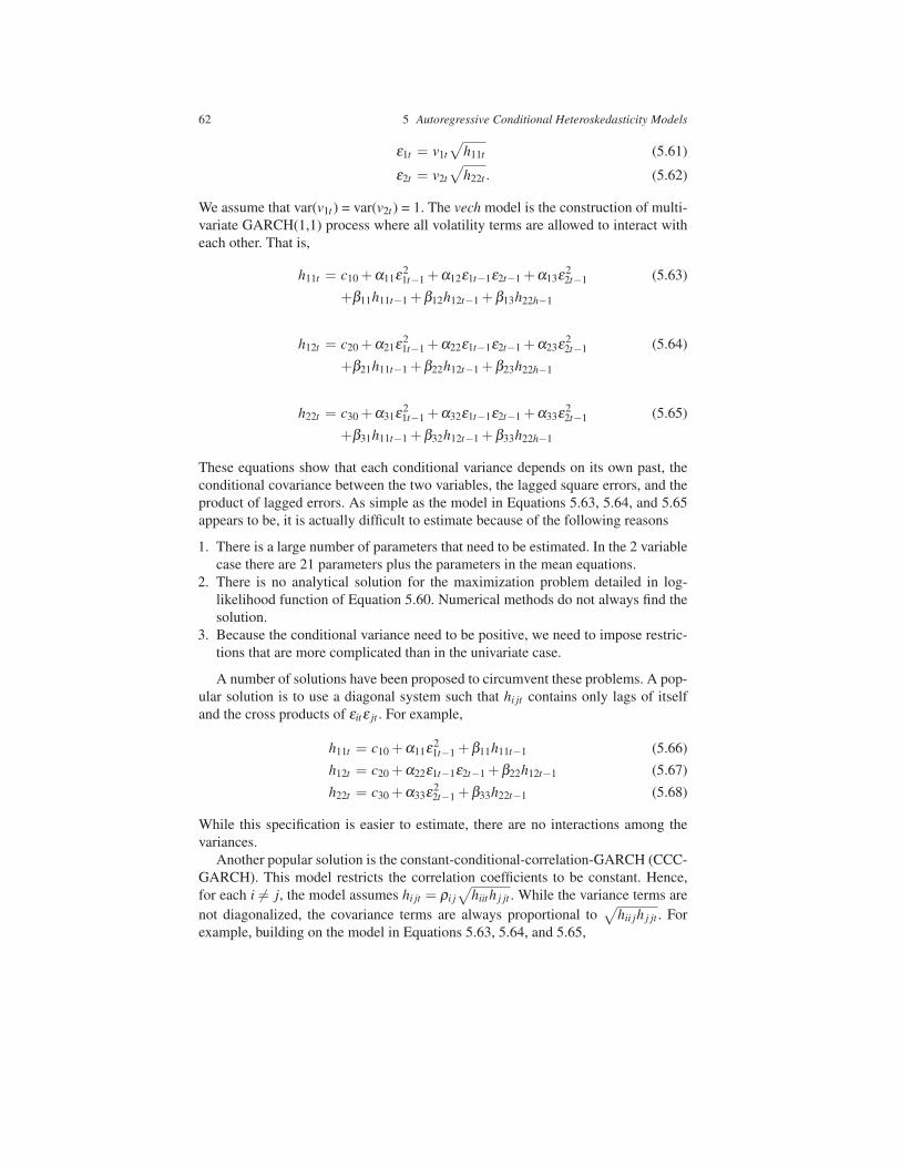
We assume that var(v1t ) = var(v2t ) = 1. The vech model is the construction of multi-
variate GARCH(1,1) process where all volatility terms are allowed to interact with
each other. That is,
h11t = c10 +α11ε21t−1 +α12ε1t−1ε2t−1 +α13ε2
2t−1 (5.63)
+β11h11t−1 +β12h12t−1 +β13h22h−1
h12t = c20 +α21ε21t−1 +α22ε1t−1ε2t−1 +α23ε2
2t−1 (5.64)
+β21h11t−1 +β22h12t−1 +β23h22h−1
h22t = c30 +α31ε21t−1 +α32ε1t−1ε2t−1 +α33ε2
2t−1 (5.65)
+β31h11t−1 +β32h12t−1 +β33h22h−1
These equations show that each conditional variance depends on its own past, the
conditional covariance between the two variables, the lagged square errors, and the
product of lagged errors. As simple as the model in Equations 5.63, 5.64, and 5.65
appears to be, it is actually difficult to estimate because of the following reasons
1. There is a large number of parameters that need to be estimated. In the 2 variable
case there are 21 parameters plus the parameters in the mean equations.
2. There is no analytical solution for the maximization problem detailed in log-
likelihood function of Equation 5.60. Numerical methods do not always find the
solution.
3. Because the conditional variance need to be positive, we need to impose restric-
tions that are more complicated than in the univariate case.
A number of solutions have been proposed to circumvent these problems. A pop-
ular solution is to use a diagonal system such that hi jt contains only lags of itself
and the cross products of εitε jt . For example,
h11t = c10 +α11ε21t−1 +β11h11t−1 (5.66)
h12t = c20 +α22ε1t−1ε2t−1 +β22h12t−1 (5.67)
h22t = c30 +α33ε22t−1 +β33h22t−1 (5.68)
While this specification is easier to estimate, there are no interactions among the
variances.
Another popular solution is the constant-conditional-correlation-GARCH (CCC-
GARCH). This model restricts the correlation coefficients to be constant. Hence,
for each i 6= j, the model assumes hi jt = ρi j
√
hiith j jt . While the variance terms are
not diagonalized, the covariance terms are always proportional to√
hii jh j jt . For
example, building on the model in Equations 5.63, 5.64, and 5.65,
5.7 Multivariate GARCH Models 63
h12t = ρ12
√
h11th22t (5.69)
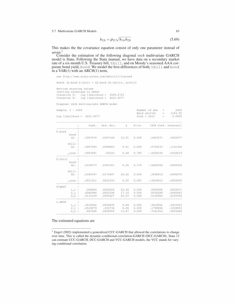
This makes the the covariance equation consist of only one parameter instead of
seven.1
Consider the estimation of the following diagonal vech multivariate GARCHmodel is Stata. Following the Stata manual, we have data on a secondary marketrate of a six-month U.S. Treasury bill, tbill, and on Moody’s seasoned AAA cor-porate bond yield, bond. We model the first-differences of both, tbill and bondin a VAR(1) with an ARCH(1) term,
use http://www.stata-press.com/data/r11/irates4
dvech (D.bond D.tbill = LD.bond LD.tbill), arch(1)
Getting starting values
(setting technique to bhhh)
Iteration 0: log likelihood = 3569.2723
Iteration 8: log likelihood = 4221.6577
Diagonal vech multivariate GARCH model
Sample: 3 - 2456 Number of obs = 2454
Wald chi2(4) = 1183.52
Log likelihood = 4221.6577 Prob > chi2 = 0.0000
------------------------------------------------------------------------------
| Coef. Std. Err. z P>|z| [95% Conf. Interval]
-------------+----------------------------------------------------------------
D.bond |
bond |
LD. | .2967674 .0247149 12.01 0.000 .2483271 .3452077
|
tbill |
LD. | .0947949 .0098683 9.61 0.000 .0754533 .1141364
|
_cons | .0003991 .00143 0.28 0.780 -.0024036 .0032019
-------------+----------------------------------------------------------------
D.tbill |
bond |
LD. | .0108373 .0301501 0.36 0.719 -.0482558 .0699304
|
tbill |
LD. | .4344747 .0176497 24.62 0.000 .3998819 .4690675
|
_cons | .0011611 .0021033 0.55 0.581 -.0029612 .0052835
-------------+----------------------------------------------------------------
Sigma0 |
1_1 | .004894 .0002006 24.40 0.000 .0045008 .0052871
2_1 | .0040986 .0002396 17.10 0.000 .0036289 .0045683
2_2 | .0115149 .0005227 22.03 0.000 .0104904 .0125395
-------------+----------------------------------------------------------------
L.ARCH |
1_1 | .4514942 .0456835 9.88 0.000 .3619562 .5410323
2_1 | .2518879 .036736 6.86 0.000 .1798866 .3238893
2_2 | .843368 .0608055 13.87 0.000 .7241914 .9625446
------------------------------------------------------------------------------
The estimated equations are
1 Engel (2002) implemented a generalized CCC-GARCH that allowed the correlations to change
over time. This is called the dynamic-conditional-correlation-GARCH (DCC-GARCH). Stata 12
can estimate CCC-GARCH, DCC-GARCH and VCC-GARCH models, the VCC stands for vary-
ing conditional correlation.
64 5 Autoregressive Conditional Heteroskedasticity Models
∆bond = 0.0004+0.296∆bondt−1 +0.095∆tbillt−1 + ε1t (5.70)
∆tbill = 0.0011+0.011∆bondt−1 +0.434∆tbillt−1 + ε2t (5.71)
H =
[
0.0048ε21t−1 +0.4515h11t−1 0.0040ε1t−1ε2t−1 +0.2519h21t−1
0.0040ε1t−1ε2t−1 +0.2519h12t−1 0.0115ε22t−1 +0.8434h22t−1
]
.
or
h11t = 0.0048ε21t−1 +0.4515h11t−1 (5.72)
h12t = 0.0040ε1t−1ε2t−1 +0.2519h12t−1 (5.73)
h22t = 0.0115ε22t−1 +0.8434h22t−1 (5.74)
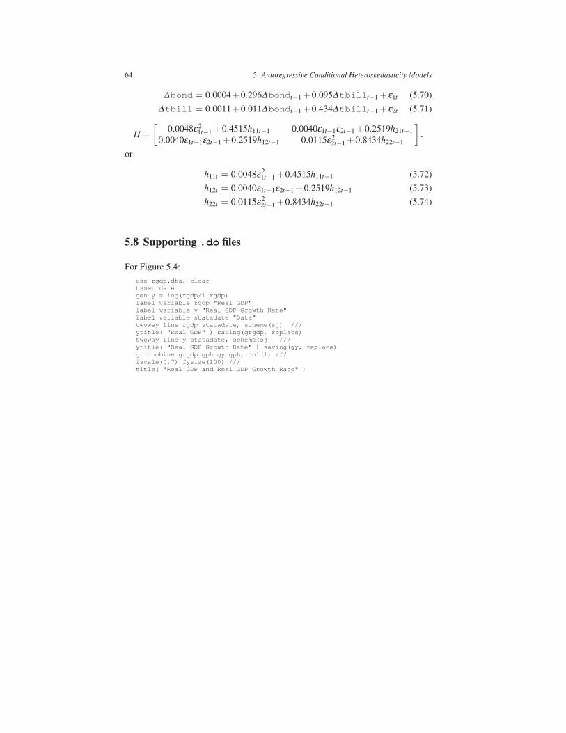
5.8 Supporting .do files
For Figure 5.4:
use rgdp.dta, clear
tsset date
gen y = log(rgdp/l.rgdp)
label variable rgdp "Real GDP"
label variable y "Real GDP Growth Rate"
label variable statadate "Date"
twoway line rgdp statadate, scheme(sj) ///
ytitle( "Real GDP" ) saving(grgdp, replace)
twoway line y statadate, scheme(sj) ///
ytitle( "Real GDP Growth Rate" ) saving(gy, replace)
gr combine grgdp.gph gy.gph, col(1) ///
iscale(0.7) fysize(100) ///
title( "Real GDP and Real GDP Growth Rate" )