STRUCTURAL AND PHYSICAL PROPERTIES OF HIGH REDSHIFT

GALAXIES IN THE HUBBLE ULTRA DEEP FIELD

by

Nimish P. Hathi

A Dissertation Presented in Partial Fulfillmentof the Requirements for the Degree

Doctor of Philosophy

ARIZONA STATE UNIVERSITY

August 2008

c© 2008 Nimish P. HathiAll Rights Reserved

STRUCTURAL AND PHYSICAL PROPERTIES OF HIGH REDSHIFT

GALAXIES IN THE HUBBLE ULTRA DEEP FIELD

by

Nimish P. Hathi

has been approved

May 2008

Graduate Supervisory Committee:

Rogier A. Windhorst, Co-ChairSangeeta Malhotra, Co-Chair

James RhoadsRolf A. JansenRichard Lebed

ACCEPTED BY THE GRADUATE COLLEGE

ABSTRACT

In the past decade, the Hubble Space Telescope has observed large numbers

of distant galaxies. Nonetheless, the process of galaxy assembly and formation at

high redshifts remains poorly constrained. There is presently little information on

structure formation and star-formation processes within these high-redshift galaxies.

This dissertation presents results from three studies in the Hubble Ultra Deep Field

(HUDF), the deepest optical data yet, to understand these distant galaxies.

The first part of this dissertation is a study of faint compact Lyman-break

galaxies (LBGs) at redshift 4 to 6 (about 1 billion years after the Big Bang) in

the HUDF. These LBGs are too faint individually to accurately measure their radial

surface brightness (SB) profiles. The HUDF images of sets of these LBGs, pre-selected

to have nearly identical compact sizes and the roundest shapes, were co-added. From

these composite images, average SB profiles were then computed that show that even

the faintest galaxies at redshift 4 to 6 are resolved and that the inner regions are best

represented by disk-like Sersic profiles.

The second part of this dissertation utilizes the deep GRism ACS Program for

Extragalactic Science (GRAPES) to spectroscopically confirm 47 LBGs at redshift 5

to 6 in the HUDF. These 47 galaxies are less dusty than galaxies at redshift 3, and

their peak star-formation rate (SFR) intensity (i.e., SFR per unit area) does not vary

significantly from that in the local universe. The constancy of this peak intensity

implies that the same physical mechanisms limit starburst intensity at all redshifts

up to 6.

iii

The third part of this dissertation uses the HUDF images and the GRAPES

spectroscopy to explore the stellar population ages of the bulges in late-type galaxies

(i.e., Hubble types Sb-Sd) at redshift one. The results show that these late-type

bulges are younger and less massive than bulges in early-type galaxies at similar

redshifts, and that these late-type bulges are better fit by an exponential than by

de Vaucouleurs SB profile. The overall picture emerging from this analysis is that, in

late-type galaxies at redshift one, bulges form from disk material rather than from a

major-merger event.

iv

This dissertation is dedicated to my wife, Purvi, and to my parents for their

unconditional love and support.

v

ACKNOWLEDGMENTS

The path towards this dissertation, carried out at the Department of Physics at

Arizona State University (ASU), spans several years of work, and many people have

been involved in and have contributed towards the presented work. I acknowledge

my debt to those who have helped along the way.

I would like to express my sincere gratitude to Rogier Windhorst, who has

been my supervisor since the beginning of my study. He provided me with many

helpful suggestions, important advice, financial support and constant encouragement

during the course of this work. He gave me many opportunities to lead proposals and

observations, and he took every possible chance he got to introduce my work to others.

I am also grateful to Sangeeta Malhotra, for her supervision, discussions, financial

support and understanding in various aspects of my research. Her suggestions and

guidance have encouraged me throughout the study. I would also thank Seth Cohen,

who was very helpful with my everyday research. I learned a lot from him and it was

fun working with him. I thank my whole committee for doing their part to make this

process worthwhile. They are Rogier Windhorst, Sangeeta Malhotra, Rolf Jansen,

James Rhoads, and Richard Lebed.

I gratefully thank my fellow graduate students who provided both emotional

support and taught me many of the important skills that I learned along the way.

In no particular order, they are Luis Echevarria, Joseph Baker, Joseph Foy, Jason

Cook, Violet Taylor, Russell Ryan, Kazuyuki Tamura, Amber Straughn, Hwihyun

Kim and Steven Finkelstein. In addition to those already mentioned, I have enjoyed

vi

working with many other excellent astronomers along the way and I thank them for

their collaboration and guidance during these years. They are Steven Odewahn, Rolf

Jansen, Haojing Yan, Michael Corbin, William Keel, James Rhoads, Norbert Pirzkal,

Chun Xu, Ignacio Ferreras, Anna Pasquali, Anton Koekemoer and Norman Grogin.

I would also thank all the rest of the academic and support staff of the De-

partment of Physics, the ASU School of Earth and Space Exploration (SESE) and

the International Student Office (ISO) for their hospitality and help during my many

years through this process.

Financial support during my research at ASU has come from various sources.

First, I thank ASU and the Physics Department for giving me Teaching Assistantship

during my initial years of my graduate studies and secondly, I would like to thank

STScI/NASA for various research grants, whose funding helped me during my thesis

work and those are HST-GO-9066, HST-GO-9780, HST-GO-9793, HST-GO-10530,

HST-AR-10298, HST-AR-11258 & HST-AR-11287 from STScI, which is operated by

AURA under NASA contract NAS5-26555. I would also like to thank the Gradu-

ate Professional Student Association (GPSA) at ASU for their travel grants for my

conference presentations.

Finally but most importantly, I thank my wife and parents, for supporting me

along the way. Your patience, love and encouragement have upheld me particularly

in those days in which I spent more time with my computer than with you. I also

appreciate the support from the rest of my family over the years.

vii

TABLE OF CONTENTS

Page

LIST OF TABLES . . . . . . . . . . . . . . . . . . . . . . . . . . . . . . . . . xi

LIST OF FIGURES . . . . . . . . . . . . . . . . . . . . . . . . . . . . . . . . xii

CHAPTER 1 INTRODUCTION . . . . . . . . . . . . . . . . . . . . . . . . . 1

1.1 Lyman Break Selection (z&3) . . . . . . . . . . . . . . . . . . . . . . 2

1.2 4000 A Break Selection (z≃1) . . . . . . . . . . . . . . . . . . . . . . 6

CHAPTER 2 SURFACE BRIGHTNESS PROFILES AT z≃4−6 . . . . . . 10

2.1 Overview . . . . . . . . . . . . . . . . . . . . . . . . . . . . . . . . . 10

2.2 Introduction . . . . . . . . . . . . . . . . . . . . . . . . . . . . . . . . 10

2.3 Observations and Sample Selection . . . . . . . . . . . . . . . . . . . 14

The z≃4 and z≃5 objects (B-, V -band dropouts) . . . . . . . 15

The z≃6 objects (i′-band dropouts) . . . . . . . . . . . . . . . 18

2.4 The HUDF Sky Surface-Brightness Level . . . . . . . . . . . . . . . . 18

2.5 Composite Surface Brightness Profiles . . . . . . . . . . . . . . . . . . 24

Test of the stacking technique on nearby galaxies . . . . . . . . 29

2.6 Discussion . . . . . . . . . . . . . . . . . . . . . . . . . . . . . . . . . 32

Galaxies with different morphologies . . . . . . . . . . . . . . 32

Central star formation/starburst . . . . . . . . . . . . . . . . 33

Limits to dynamical ages for z≃4, 5, 6 objects . . . . . . . . . 34

2.7 Looking Towards the Future (JWST Science) . . . . . . . . . . . . . . 36

viii

Page

CHAPTER 3 STARBURST INTENSITY LIMIT AT z≃5−6 . . . . . . . . 38

3.1 Overview . . . . . . . . . . . . . . . . . . . . . . . . . . . . . . . . . 38

3.2 Introduction . . . . . . . . . . . . . . . . . . . . . . . . . . . . . . . . 38

3.3 Observations and Sample Selection . . . . . . . . . . . . . . . . . . . 40

3.4 Starburst Intensity Limit (Effective Surface Brightness) . . . . . . . . 46

Magnitudes and color measurements . . . . . . . . . . . . . . 46

The UV spectral slope (β) . . . . . . . . . . . . . . . . . . . . 47

Half-light radius (re) measurements . . . . . . . . . . . . . . . 49

Calculation of surface brightness for starburst galaxies . . . . 50

3.5 Starburst Intensity Limit (Brightest Pixel) . . . . . . . . . . . . . . . 53

3.6 Results and Discussion . . . . . . . . . . . . . . . . . . . . . . . . . . 56

Selection and measurement effects . . . . . . . . . . . . . . . . 56

The starburst intensity limit . . . . . . . . . . . . . . . . . . . 58

Size and luminosity evolution . . . . . . . . . . . . . . . . . . 61

Evolution in UV spectral slope (β) . . . . . . . . . . . . . . . . 62

CHAPTER 4 LATE-TYPE GALAXIES AT z≃1 . . . . . . . . . . . . . . . 64

4.1 Overview . . . . . . . . . . . . . . . . . . . . . . . . . . . . . . . . . 64

4.2 Introduction . . . . . . . . . . . . . . . . . . . . . . . . . . . . . . . . 64

4.3 Observations and Sample Selection . . . . . . . . . . . . . . . . . . . 68

The HST/ACS data . . . . . . . . . . . . . . . . . . . . . . . 68

Sample selection and properties . . . . . . . . . . . . . . . . . 69

ix

Page

Observed color profiles . . . . . . . . . . . . . . . . . . . . . . 75

4.4 Morphological Properties . . . . . . . . . . . . . . . . . . . . . . . . . 77

CAS measurements . . . . . . . . . . . . . . . . . . . . . . . . 78

Two-dimensional (2D) galaxy fitting using GALFIT . . . . . . 78

4.5 Stellar Population Models . . . . . . . . . . . . . . . . . . . . . . . . 83

Star formation histories (SFH) . . . . . . . . . . . . . . . . . 83

Bulge mass estimates . . . . . . . . . . . . . . . . . . . . . . . 91

Disk contamination . . . . . . . . . . . . . . . . . . . . . . . . 92

4.6 Discussion . . . . . . . . . . . . . . . . . . . . . . . . . . . . . . . . . 95

CHAPTER 5 DISCUSSION & CONCLUSIONS . . . . . . . . . . . . . . . . 101

5.1 Overview . . . . . . . . . . . . . . . . . . . . . . . . . . . . . . . . . 101

5.2 Summary of Results . . . . . . . . . . . . . . . . . . . . . . . . . . . 101

Surface brightness profiles at z≃4−6 (chapter 2) . . . . . . . 101

Starburst intensity limit at z≃5−6 (chapter 3) . . . . . . . . 103

Late-type galaxies at z≃1 (chapter 4) . . . . . . . . . . . . . . 104

5.3 Future Work . . . . . . . . . . . . . . . . . . . . . . . . . . . . . . . 104

Starburst activity and stellar population at z≃5−6 . . . . . . 106

Surface brightness (SB) profiles of galaxies at z≃4–6 . . . . . 108

REFERENCES . . . . . . . . . . . . . . . . . . . . . . . . . . . . . . . . . . 111

x

LIST OF TABLES

Table Page

1 Measured Sky Values in HUDF BV i′z′ Filters . . . . . . . . . . . . . 24

2 Measured Sky Surface Brightness in HUDF . . . . . . . . . . . . . . . 25

3 Dynamical Ages for z≃4 − 6 Objects . . . . . . . . . . . . . . . . . . 29

4 Sample of z≃4−6 Galaxies . . . . . . . . . . . . . . . . . . . . . . . 43

5 Sample Properties of z≃1 Galaxies . . . . . . . . . . . . . . . . . . . 72

6 Redshifts for Sample Galaxies at z≃1 . . . . . . . . . . . . . . . . . 73

xi

LIST OF FIGURES

Figure Page

1. Model spectra of a dropout galaxy at z≃6 . . . . . . . . . . . . . . . 5

2. Example of the dropout galaxy at z≃6 . . . . . . . . . . . . . . . . . 5

3. The HUDF number counts for all z≃4, 5, 6 objects . . . . . . . . . . 15

4. Ellipticity, (1 − b/a), versus FWHM, for all z≃4, 5, 6 objects . . . . . 17

5. Distribution of modal sky background (from object stamps) . . . . . 21

6. The actual sky values in BV i′z′ from flat-fielded HUDF exposures . . 22

7. Distribution of modal sky background (from blank stamps) . . . . . . 23

8. Composite surface brightness profiles . . . . . . . . . . . . . . . . . . 26

9. Composite images for z≃4, 5, 6 objects . . . . . . . . . . . . . . . . . 27

10. Mean surface brightness profile for z≃4, 5, 6 objects . . . . . . . . . 28

11. Stacking test on nearby galaxies . . . . . . . . . . . . . . . . . . . . . 31

12. UV spectral slopes (β) vs. redshift relation . . . . . . . . . . . . . . . 48

13. Size vs. redshift relation . . . . . . . . . . . . . . . . . . . . . . . . . 50

14. Bolometric luminosity and effective surface brightness against effective

radii for starburst galaxies . . . . . . . . . . . . . . . . . . . . . . . . 53

15. Bolometric effective surface brightness as a function of redshift . . . . 54

16. Brightest pixel surface brightness as a function of redshift . . . . . . . 55

17. Distribution of amplitude of 4000 A break (D4000) . . . . . . . . . . 71

18. Color composite images of 6 galaxies at z≃1 . . . . . . . . . . . . . . 71

19. Observed (V –z′) colors of 6 galaxies at z≃1 . . . . . . . . . . . . . . 76

xii

Figure Page

20. Observed (V –i′) colors vs. redshift for bulges and spheroids . . . . . . 77

21. Asymmetry and Concentration for selected galaxies at z≃1 . . . . . . 79

22. Distribution of Sersic indices (n) for our galaxies at z≃1 . . . . . . . 82

23. The distribution of bulge metallicities . . . . . . . . . . . . . . . . . . 86

24. Spectral energy distributions of 10 galaxies in our sample . . . . . . . 87

25. The 4000 A break amplitude as a function of stellar age . . . . . . . . 88

26. Ages and metallicities for selected galaxies at z≃1 . . . . . . . . . . . 89

27. Formation redshift (zF ) and the e-folding timescale (τf) from models 91

28. Comparison between aperture colors, B/D ratio and the bulge age . . 94

29. Correlation between measured B/D ratio with bulge ages and masses. 95

30. Comparison between bulges in early-type and late-type galaxies . . . 97

xiii

1. INTRODUCTION

In the past decade, space-based and ground-based observations of high redshift

galaxies have begun to outline the process of galaxy assembly. The details of that

process at high redshifts, however, remain poorly constrained. There are two major

— somewhat contradicting — scenarios of galaxy assembly and formation. Many

observational and theoretical predictions favor a hierarchical picture of galaxy forma-

tion, in which galaxies we observe locally were built-up by a series of mergers from

smaller building blocks (e.g., Yan & Windhorst 2004a; Ferguson et al. 2004; Ryan et

al. 2007), while in an alternate ‘anti’-hierarchical scenario, the most massive galaxies

assemble earlier than their less massive counterparts (e.g., Cowie et al. 1996; Heavens

et al. 2004; Panter et al. 2007). The only way to test these or similar scenarios, and

to constrain their details, is to obtain deep multi-color imaging and study distant

galaxies while they undergo such processes.

In the last decade, major deep high-resolution imaging surveys, such as the

Hubble Deep Fields (HDF; Williams et al. 1996), the Great Observatories Origins

Deep Survey (GOODS; Giavalisco et al. 2004a), the Galaxy Evolution from Mor-

phology and SEDs (GEMS; Rix et al. 2005), the Hubble Ultra Deep Field (HUDF;

Beckwith et al. 2006), the All-wavelength Extended Groth Strip International Sur-

vey (AEGIS; Davis et al. 2007), and the Cosmological Evolution Survey (COSMOS;

Scoville et al. 2007), have increased the availability of deep imaging manifold. It is no

longer possible to obtain ground-based spectroscopic identification for every source

in a field, both due to the huge number of sources in a field and due to the faintness

of these distant sources.

2

Photometric redshift techniques use broad-band photometry obtained through

various band-passes (filters) to estimate (the observed) Spectral Energy Distributions

(SEDs) of each galaxy. These observed SEDs are in a sense very low resolution

spectra that can be compared to theoretical SEDs to estimate the redshifts and the

intrinsic properties of distant galaxies. Therefore, photometric redshifts estimated

from observed fluxes are an important tool for the statistical study of distant galaxies

(e.g., Fernandez-Soto et al. 1999; Benitez 2000; Mobasher et al. 2004, 2007; Ryan

et al. 2007). Details of this technique are described in, e.g., Ryan et al. (2007).

The success of photometric redshift techniques heavily relies on observing either of

the two strongest spectral features (breaks) in the observed galaxy SEDs. These

are the Lyman-break (below rest-frame 1216 A) and the 4000 A break (due to the

combination of the Balmer break at 3646 A, higher order Balmer absorption lines

and absorption by ionized metals especially Ca II H-K). These two spectral breaks

are very useful to identify distant (z & 1) galaxies, because at these redshifts, these

breaks are redshifted into the observed optical/near-infrared band-passes, which are

most observed in major imaging surveys. This dissertation is based on three different

studies of distant (z & 1) galaxies selected by their Lyman and 4000 A breaks as

discussed in following two sections.

1.1. Lyman Break Selection (z&3)

The Lyman-break technique (Steidel & Hamilton 1992; Steidel et al. 1996a)

has been widely used to select galaxies at high redshifts (z &3). This method relies

on multi-band imaging to identify the redshifted, characteristic discontinuity — the

3

Lyman-break — in the SED of high-redshift galaxies, which is largely caused by

the Lyman limit and Lyman-α absorption (λrest . 1216 A) of far-Ultraviolet (UV)

photons by intervening neutral hydrogen along the sight-lines to such galaxies (e.g.,

Madau 1995). This technique requires imaging in at least two passbands, one to the

blue side of the break and the other to the red side. The presence of a Lyman-break

makes high-redshift galaxies much fainter in the blue band than in the red one, or

in other words, it makes them appear to “drop-out” from the blue band. For this

reason, this method is also known as the drop-out selection, and the candidates found

in this way are generally referred to as “dropouts”.

The ‘classical’ Lyman-break technique used by Steidel et al. (1996a) uses three

filters: one redward of rest frame Lyman-α (λrest > 1216 A), a second in the spectral

region between rest frame Lyman-α and the rest frame Lyman limit (912 A), and a

third at λrest < 912 A. At z ≃ 3, the technique relies on the ubiquitous step in the

spectra of the stellar component of galaxies at 912 A. The photons emitted by the

galaxy at wavelengths bluer than the Lyman limit are capable of ionizing neutral hy-

drogen, and thus are quickly absorbed by even a slight amount of intervening neutral

hydrogen in the intergalactic medium (IGM) along the sight-line. This Lyman-break

technique was first applied to galaxies at z≃3. At these redshifts, the strongest drop

in the flux level occurs at/below restframe 912 A, which in the observer’s frame occurs

in UV filters, such as F300W on the Hubble Space Telescope (HST ), or the ground-

based U -band at slightly longer wavelengths (∼3600 A). Because the break occurs

in the U -band, these galaxies are also called U -band dropouts. At higher redshifts

4

(z≃4 and beyond), there are more intervening neutral hydrogen clumps between the

observer and a galaxy, and the Lyman-α absorption forest (between Ly-α and Ly-β)

and the Lyman-β absorption forest (between Ly-β and Lyman limit) — due to thick

intervening neutral hydrogen clouds — becomes so dense that most of the UV contin-

uum blueward of rest-frame 1216 A will be absorbed (see Madau 1995). As we move

to higher redshifts, this break travels into optical bands redwards of the U -band and

therefore, for galaxies at z≃4 (3.5≤ z≤4.4) it occurs in the B-band (F435W). This

galaxy population at z≃ 4 is also called the “B-band dropouts”. Similarly, galaxies

at z≃5 (4.5≤z≤5.4) are referred to as “V -band (F606W) dropouts”.

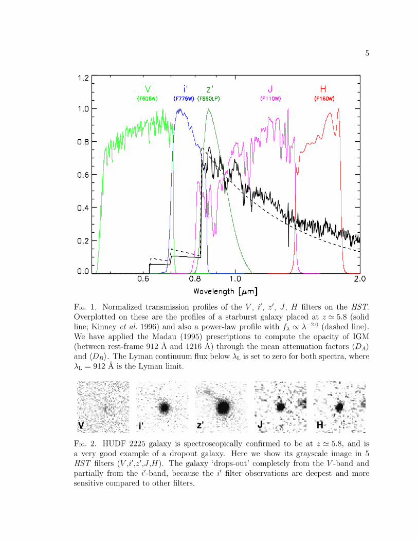
As its first application in the z≃6 regime, Yan et al. (2003, hereafter YWC03)

used this technique in a deep field observed by the Advanced Camera for Surveys

(ACS) in the default pure parallel mode (Sparks et al. 2001) soon after its deployment

on-board the HST. In this redshift range, the Lyman-break occurs at around 8512 A

in the observer’s frame, which is well bracketed by the i′ (F775W) and z′ (F850LP)

filters (as shown in Figure 1), through which this deep parallel field was imaged.

YWC03 found a significant number of i′-band dropouts, and argued that the vast

majority of them were very likely galaxies at z≃6.

Many recent surveys have found a large numbers of these dropouts, which

are candidate galaxies at z & 4. The HUDF, GOODS and deep ACS parallel fields

contain &500 objects (Yan & Windhorst 2004a,b; Beckwith et al. 2006; Bouwens et

al. 2006, 2007) which are B, V , or i′-band dropouts, making them candidates for

galaxies at z≃4, 5, 6, respectively. Figure 2 shows an example of a dropout galaxy at

5

FIG. 1. Normalized transmission profiles of the V , i′, z′, J , H filters on the HST.Overplotted on these are the profiles of a starburst galaxy placed at z ≃ 5.8 (solidline; Kinney et al. 1996) and also a power-law profile with fλ ∝ λ−2.0 (dashed line).We have applied the Madau (1995) prescriptions to compute the opacity of IGM(between rest-frame 912 A and 1216 A) through the mean attenuation factors 〈DA〉and 〈DB〉. The Lyman continuum flux below λL is set to zero for both spectra, whereλL = 912 A is the Lyman limit.

FIG. 2. HUDF 2225 galaxy is spectroscopically confirmed to be at z ≃ 5.8, and isa very good example of a dropout galaxy. Here we show its grayscale image in 5HST filters (V ,i′,z′,J ,H). The galaxy ‘drops-out’ completely from the V -band andpartially from the i′-band, because the i′ filter observations are deepest and moresensitive compared to other filters.

6

z≃5.8 in the HUDF. The majority of the galaxies at z &4 are not spectroscopically

confirmed in these studies, and are selected purely on the basis of their broad-band

colors. This selection can cause the samples to be contaminated by lower redshift,

dusty elliptical galaxies and foreground Galactic stars with similar broad-band colors.

Details regarding some of the possible interlopers in selecting galaxies at z≃5−6 are

discussed in the literature (e.g., YWC03; Ryan et al. 2005; Yan et al. 2008). The

candidate galaxies at z ≃ 5−6 are comparatively fainter than most interlopers, and

most of the major survey fields are located at higher galactic latitudes, where the

surface density of galactic stars is very low. Therefore, we expect only a relatively

small fraction (<10%; Vanzella et al. 2006) of contaminants in the sample of dropouts.

There is presently little information on the dynamical structure/morphology

of faint galaxies at z & 4. It is not clear whether these objects represent isolated

disk systems, or collapsing spheroids, mergers or other dynamically young objects.

In chapter 2 of this dissertation, we investigate faint high-redshift (z≃4−6) dropout

galaxies in the HUDF to understand their structure, morphology and stellar popu-

lations. In chapter 3, we take a sub-sample of these high redshift dropout galaxies

— with spectroscopically confirmed redshifts from the HST/ACS low resolution faint

grism spectroscopy — and compare their intrinsic physical properties with their lower

redshift counterparts.

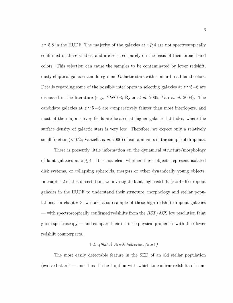
1.2. 4000 A Break Selection (z≃1)

The most easily detectable feature in the SED of an old stellar population

(evolved stars) — and thus the best option with which to confirm redshifts of com-

7

paratively older z≃1 galaxies (e.g., ellipticals, spiral bulges) — is the 4000 A break.

The 4000 A break is due to absorption in the atmospheres of stars and arises because of

an accumulation of absorption lines of mainly ionized metals and higher-order Balmer

lines. As the opacity increases with decreasing stellar temperature, the 4000 A break

gets stronger with older ages. This makes the 4000 A break a powerful diagnostic in

stellar population studies (e.g., Pasquali et al. 2006b; Hathi et al. 2008c).

Bulges in spiral galaxies were historically thought to be elliptical galaxies that

happen to have a disk of stars around them. Recent high resolution images, using

HST, reveal that many bulges have properties that more closely resemble disk galaxies.

It is now thought that there are at least two types of bulges, bulges that are like

elliptical galaxies (classical bulges) and bulges that are like disk galaxies (disky bulges

or pseudo bulges). Detailed discussion on these two classes of bulges is given in the

review by Kormendy & Kennicutt (2004). Based on this differentiation of bulges,

there are currently two alternative scenarios to explain bulge formation in galaxies.

First, semi-analytic models have traditionally proposed early formation from mergers,

generating a scaled-down version of an elliptical galaxy (e.g., Kauffmann et al. 1993).

Second, dynamical instabilities can contribute to the formation of a bulge within

a primordial disk (e.g., Kormendy & Kennicutt 2004). These instabilities can be

triggered either internally or by the accretion of small satellite galaxies (Hernquist

& Mihos 1995), and may result in later stages of star formation (e.g., Kannappan et

al. 2004). Hence, studies of the stellar populations in galaxy bulges provide valuable

constraints to distinguish between these two scenarios.

8

The ability of HST to spatially resolve distant galaxies enabled the study of

bulges in galaxies out to redshift z≃1 (Bouwens et al. 1999; Abraham et al. 1999; Ellis

et al. 2001; Menanteau et al. 2001; Koo et al. 2005; MacArthur et al. 2008). Based

on an analysis of HST data on distant galaxies, Bouwens et al. (1999) specified three

basic bulge formation scenarios: (1) a secular evolution model in which bulges form

after disks and undergo several central starbursts; (2) a primordial collapse model in

which bulges and disks form simultaneously; and (3) an early bulge-formation model

in which bulges form prior to disks. Models 1 and 2 both predict that a large fraction

of distance bulges are luminous and relatively blue, while model 3 predicts mainly

very red bulges. The advantage of the lookback time probed out to z ≃ 1 allows us

to quantify the occurrence of merging vs. secular formation of bulges.

In the sample presented in Chapter 4 of this dissertation, we take advantage of

the superb capabilities of the HST/ACS to extract (slitless) low-resolution spectra of

bulges within late-type galaxies (i.e., Hubble types Sb-Sd) to understand their stellar

population and how these galaxies assemble at z≃1.

This dissertation is organized as follows: the contents of Chapter 2 have ap-

peared as Hathi, N. P., et al. 2008, AJ, 135, 156 (copyrighted and published by the

American Astronomical Society in January 2008 issue of The Astronomical Journal),

while the contents of Chapter 3 have appeared as Hathi, N. P., et al. 2008, ApJ, 673,

686 (copyrighted and published by the American Astronomical Society in March 2008

issue of The Astrophysical Journal). The contents of Chapter 4 have been accepted to

appear as Hathi, N. P., et al. 2008 in the Astrophysical Journal (will be copyrighted

9

and published by the American Astronomical Society). Chapter 5 summarizes im-

portant results of this dissertation and present possible future research directions to

be pursued.

2. SURFACE BRIGHTNESS PROFILES AT z≃4−6

2.1. Overview

The Hubble Ultra Deep Field (HUDF) contains a significant number of B-,

V - and i′-band dropout objects, many of which were recently confirmed to be young

star-forming galaxies at z ≃ 4−6. These galaxies are too faint individually to accu-

rately measure their radial surface brightness profiles. Their average light profiles are

potentially of great interest, since they may contain clues to the time since the onset

of significant galaxy assembly. We separately co-add V , i′- and z′-band HUDF images

of sets of z≃4, 5 and 6 objects, pre-selected to have nearly identical compact sizes and

the roundest shapes. From these stacked images, we are able to study the averaged

radial structure of these objects at much higher signal-to-noise ratio than possible for

an individual faint object. Here we explore the reliability and usefulness of a stacking

technique of compact objects at z ≃ 4−6 in the HUDF. Our results are: (1) image

stacking provides reliable and reproducible average surface brightness profiles; (2) the

shape of the average surface brightness profile shows that even the faintest z≃4−6

objects are resolved at the HST diffraction limit in the red (∼0′′.08 FWHM); and (3)

if late-type galaxies dominate the population of galaxies at z≃4−6, as previous HST

studies have shown for z.4, then limits to dynamical age estimates for these galax-

ies from their profile shapes are comparable with the Spectral Energy Distribution

(SED) ages obtained from the broadband colors. We also present accurate measure-

ments of the sky-background in the HUDF and its associated 1σ uncertainties.

2.2. Introduction

In the last decade, ground and space based observations of high redshift galax-

ies have begun to outline the process of galaxy assembly. The details of that process

11

at high redshifts, however, remain poorly constrained. There is increasing support for

the model of galaxy formation, in which the most massive galaxies assemble earlier

than their less massive counterparts (e.g., Cowie et al. 1996; Guzman et al. 1997; Ko-

dama et al. 2004; McCarthy et al. 2004). A detailed analysis of the ‘fossil record’ of

the current stellar populations in nearby galaxies selected from the Sloan Digital Sky

Survey (SDSS; York et al. 2000) provides strong evidence for this downsizing picture

(Heavens et al. 2004; Panter et al. 2007). The increasing number of luminous galaxies

spectroscopically confirmed to be at z≃6.5 (e.g., Hu et al. 2002; Kodaira et al. 2003;

Kurk et al. 2004; Rhoads et al. 2004; Stern et al. 2005; Taniguchi et al. 2005), or .0.9

Gyr after the Big Bang, also supports this general picture. In an alternate hierar-

chical scenario, arguments have been made that significant number of low luminosity

dwarf galaxies were present at these times, and were the main contributor to finish

the process of reionization of the intergalactic medium (Yan & Windhorst 2004a,b).

However, there is presently little information on the dynamical structure of these or

other galaxies at z ≃ 6. It is not clear whether these objects represent isolated disk

systems, or collapsing spheroids, mergers or other dynamically young objects.

Ravindranath et al. (2006) used deep, multi-wavelength images obtained with

the Hubble Space Telescope (HST ) Advanced Camera for Surveys (ACS) as part of the

Great Observatories Origins Deep Survey (GOODS) to analyze 2-D surface brightness

distributions of the brightest Lyman-break galaxies (LBGs) at 2.5<z<5. They dis-

tinguish various morphologies based on the Sersic index n, which measures the shape

of the azimuthally averaged surface brightness profile (where n=1 for exponential

12

disks and n=4 for a de Vaucouleurs law). Ravindranath et al. (2006) find that 40% of

the LBGs have light profiles close to exponential, as seen for disk galaxies, and only

∼30% have high n, as seen in nearby spheroids. They also find a significant fraction

(∼30%) of galaxies with light profiles shallower than exponential, which appear to

have multiple cores or disturbed morphologies, suggestive of close pairs or on-going

galaxy mergers. Distinction between these possible morphologies and, therefore, a

better estimate of the formation redshifts of the systems observed at z≃4−6 in par-

ticular, is important for testing the galaxy assembly picture, and for the refinement

of galaxy formation models.

One possible technique involves the radial surface brightness profiles of the

most massive objects — those that will likely evolve to become the massive elliptical

galaxies, which we see in place at redshifts z .2 (Driver et al. 1998; van Dokkum et

al. 2003, 2004). This can be analytically understood in the context of the Lynden-

Bell (1967) relaxation formalism and the numerical galaxy formation simulations of

van Albada (1982), which describe collisionless collapse and violent relaxation as the

formation mechanism for elliptical galaxies. As the time-scale for relaxation is shorter

in the inner than in the outer parts of a galaxy, convergence toward a r1/n-profile

will proceed from the inside to progressively larger radii at later times. Moreover,

Kormendy (1977) has shown that tidal perturbations due to neighbors can cause the

radial surface brightness profile to deviate from a pure de Vaucouleurs profile in the

outer parts of a galaxy. This implies that the radius where surface brightness profiles

start to deviate significantly from an r1/n profile might serve as a “virial clock” that

13

traces the time since the onset of the last major merger, accretion events or global

starburst in these objects.

Image stacking methods have been used extensively on X-ray (Brandt et al.

2001; Nandra et al. 2002) and radio (Georgakakis et al. 2003; White et al. 2007) data

to study the mean properties (e.g., flux, luminosity) of well-defined samples of sources

that are otherwise too faint to be detected individually. Pascarelle et al. (1996) applied

such a stacking method to a large number of optically very faint, compact objects at

z=2.39 to trace their “average” structure. This approach was also applied by Zibetti

et al. (2004) to detect the presence of faint stellar halos around disk galaxies selected

from the SDSS. An attempt to apply this technique to high redshift galaxies in the

Hubble Deep Field (HDF; Williams et al. 1996) was not conclusive (H. Ferguson;

private communication) due to the poorer spatial sampling and shallower depth of

the HDF/WFPC2 compared to the HUDF/ACS (Beckwith et al. 2006).

For this project, we use the exceptional depth and fine spatial sampling of

the HUDF to study the potential of this image stacking technique, and will estimate

limits to dynamical ages of faint, young galaxies at z ≃ 4−6. The HUDF reaches

∼1.5 mag deeper than the equivalent HDF exposure in the i′-band, and has better

spatial sampling than the HDF. The HUDF depth also allows us to characterize

the sky background very accurately, which is critical for successfully using a stacking

method to measure the mean surface-brightness profiles for these faint young galaxies.

Throughout this chapter we refer to the HST/ACS F435W, F606W, F775W,

and F850LP filters as the B-, V -, i′-, and z′-bands, respectively. We assume a Wilkin-

14

son Microwave Anisotropy Probe (WMAP) cosmology of Ωm=0.24, ΩΛ=0.76 and

H0=73 km s−1 Mpc−1, in accord with the most recent 3-year WMAP results of

Spergel et al. (2007). This implies a current age for the Universe of 13.7 Gyr. All

magnitudes are given in the AB system (Oke & Gunn 1983).

2.3. Observations and Sample Selection

The HUDF contains &100 objects that are i′-band dropouts, making them

candidates for galaxies at z≃6 (Bouwens et al. 2004a, 2006; Bunker et al. 2004; Yan

& Windhorst 2004b). Similarly, there are larger numbers of objects in the HUDF

that are B-band dropouts (415 in total) or V -band dropouts (265 in total), and

are candidates for galaxies at z ≃ 4 and z ≃ 5, respectively. Beckwith et al. (2006)

and Bouwens et al. (2007) find similar number of B- and V -band dropouts in the

HUDF. A significant fraction of these objects to AB.27 mag have recently been

spectroscopically confirmed to have redshifts z≃ 4−6 through the detection of Lyα

emission or identifying their Lyman break (Malhotra et al. 2005; Dow-Hygelund et al.

2007). We discuss our detailed drop-out selection criteria below. Despite the depth

(AB.29.5 mag) of the HUDF images, however, these objects appear very faint and

with little, if any, discernible structural detail. Visual inspection of all these objects

shows their morphologies to divide into four broad categories: symmetric, compact,

elongated, and amorphous.

We construct three separate catalogs for these z ≃ 4, 5, 6 galaxy candidates,

selecting only the isolated, compact and symmetric galaxies. We exclude objects

with obvious nearby neighbors, to avoid a bias due to dynamically disturbed objects

15

and complications due to chance superpositions. Figure 3 demonstrates that our

completeness limit for z≃4 and z≃5 objects is AB.29.3 mag, and for z≃6 objects

it is AB.29.0 mag. Therefore, all three catalogs are complete to AB.29.0 mag, which

is equivalent to at least a 10σ detection for objects that are nearly point sources. For

each object in our z ≃ 4, 5, 6 samples, we extracted 51×51 pixel postage stamps

(which at 0′′.03 pix−1 span 1′′.53 on a side) from the HUDF V , i′ and z′-band images,

respectively. Each postage stamp was extracted from the full HUDF, such that the

centroid of an object (usually coincident with the brightest pixel) was at the center

of that stamp.

FIG. 3. The HUDF number countsfor all z ≃ 4, 5, 6 objects beforethe sub-selection of compact iso-lated z≃4, 5, 6 objects were made.The vertical dotted line shows themagnitude to which the numbercounts of all these redshifts arecomplete. The area of the HUDFis 3.15×10−3 deg2.

The z ≃ 4 and z ≃ 5 objects (B-, V -band dropouts). — We used the i′-band

selected BV i′z′ HUDF catalog (Beckwith et al. 2006) to select the z ≃ 4 and z ≃ 5

objects. With the HyperZ code (Bolzonella et al. 2000), we computed photometric

redshift estimates, using the magnitudes and associated uncertainties tabulated in

16

the HUDF catalog. All objects with 3.5≤zphot≤4.4 were assigned to the bin of z≃4

candidates, and all objects with 4.5≤zphot≤5.4 to the bin of z≃5 candidates.

We then applied color criteria, similar to those adopted by Giavalisco et al.

(2004b), to select the B(z≃4) and V (z≃5) dropout samples. For B-band dropouts,

we require:

(B − V ) ≥ 1.2 + 1.4 × (V − z′) mag

and (B − V ) ≥ 1.2 mag

and (V − z′) ≤ 1.2 mag

For V -band dropouts, the following color selection was applied:

(V − i′) > 1.5 + 0.9 × (i′ − z′) or (V − i′) > 2.0 mag

and (V − i′) ≥ 1.2 mag

and (i′ − z′) ≤ 1.3 mag

We note, that only objects satisfying both color and photometric redshift criteria

were selected in our samples. Vanzella et al. (2006) using VLT/FORS2 observed

∼100 B-, V - and i′-band dropout objects in the Chandra Deep Field South (CDFS)

selected based on above mentioned color criteria (Giavalisco et al. 2004b). They have

spectroscopically confirmed >90% of their high redshift galaxy candidates. Therefore,

we expect only a small number (<10%) of contaminants in our sample of dropouts.

One or two objects in our final sample could be such contaminants, but because we

have 3 different realizations of 10 objects (3×10), each showing similar profiles, they

do not appear to affect our results.

The z ≃ 4 sample has 415 objects, while the z ≃ 5 sample has 265 objects.

In Figure 4ab, we show the distribution of the full-width half maximum (FWHM)

17

and ellipticity, ǫ = (1− b/a), measured in each of the two samples using SExtractor

(Bertin & Arnouts 1996). We further constrained our samples by imposing limits

on compactness and on roundness of FWHM ≤ 0′′.3 and ǫ ≤ 0.3. Again, this is to

minimize the probability that the z ≃ 4−5 candidates are significantly dynamically

disturbed, and to maximize the probability of selecting physically similar objects.

Our goal is to find the visibly most symmetric, least disturbed systems for the current

study. This sub-selection leaves 204 objects in the z ≃ 4 sample and 102 objects in

the z ≃ 5 sample. Most of these objects are faint, and are only a few pixels across

in size, and, hence, have larger uncertainties in their measurements of FWHM and

ellipticity. Therefore, we also checked our objects visually to eliminate any possibility

of our selected objects being contaminated by unrelated nearby objects, being clearly

extended, or objects with complex morphologies.

FIG. 4. Ellipticity, (1 − b/a), versus object FWHM, for all z ≃ 4 (a), z ≃ 5 (b) andz≃6 (c) objects selected in the HUDF. Measurements were performed in i′-band forz≃4 and z≃5 objects, while we used the z′-band for z≃6 objects. The FWHM ofa stellar image/PSF is ∼3 pixels or 0′′.09, indicated by the leftmost hatched area ineach panel. Objects within the shaded area meet our additional selection criteria onroundness (ǫ ≤ 0.3) and compactness (FWHM ≤ 0′′.3 or 10 pixels).

18

The z ≃ 6 objects (i′-band dropouts). — Yan & Windhorst (2004b) found

108 possible 5.5≤ z ≤6.5 candidates in the HUDF to mAB(z850)=30.0 mag. Bunker

et al. (2004) independently found the brightest 54 of these 108 z ≃ 6 candidates

to AB=28.5 mag. Similarly, deep HST/ACS grism spectra of the HUDF i′-band

dropouts confirm &90% of these objects at AB.27.5 mag to be at z ≃ 6 (Malhotra

et al. 2005; Hathi et al. 2008a). Using the catalog of Yan & Windhorst (2004b), we

extracted 108 postage stamps (51×51 pixels in size), from the HUDF z′-band image.

Like for the z ≃ 4 and z ≃ 5 objects, for each z ≃ 6 object we measured its

z′-band FWHM and ellipticity using SExtractor. Figure 4c shows the measured

ellipticity versus FWHM for all 108 z≃6 candidates. A smaller sample of 67 objects

satisfies our constraints on the FWHM and ellipticity. Further visual inspection, to

make sure that our sample has only isolated, compact and round objects, leaves 30

objects in our z≃6 sample. We therefore imposed a sample size of 30 objects also on

the two lower redshift bins after visual inspection.

The results in this project are therefore based on approximately (30/415)∼7%,

(30/265)∼11%, and (30/108)∼28% of the total z≃4, 5 and 6 galaxy populations.

2.4. The HUDF Sky Surface-Brightness Level

For the present work, it is critical that we accurately characterize the sky-

background, and correctly propagate the true 1σ errors due to the subtraction of this

sky-background. In the following, we will pursue two complimentary approaches to

determine the sky surface-brightness, and compare the results. Here, we discuss the

z′-band measurements in detail.

19

We first measured the sky-background in each of the 415 z≃4 object stamps

(‘local’ sky measurements). The Interactive Data Language (IDL1) procedure SKY2

was used to measure the sky-background. This procedure is adapted from the DAOPHOT

(Stetson 1987) routine of the same name and works as follows. First, the average and

sigma are obtained from the sky pixels. Second, these values are used to eliminate

outliers with a low probability. Third, the values are then recomputed and the process

is repeated up to 20 iterations. If there is a contamination due to an object, then the

contamination is estimated by comparing the mean and median of the remaining sky

pixels to get the true sky value. The output of this procedure is the modal sky-level

in the image.

Figure 5c shows a histogram of the z′-band modal sky values obtained from all

415 object stamps extracted from the drizzled HUDF images. The 1σ uncertainty in

the sky, σsky, determined from a Gaussian fit to the histogram, is 2.19×10−5 electrons

sec−1 in the z′-band. The sky-background level within the HUDF was obtained from

the original flat-fielded ACS images, because the final co-added HUDF data products

are sky-subtracted. The header parameters MDRIZSKY and EXPTIME were used

to obtain the actually observed sky-value. MDRIZSKY is the sky value in electrons

(e−) computed by the MultiDrizzle code (Koekemoer et al. 2002), while EXPTIME

is the total exposure time for the image in seconds, so that the average sky-value in

the HUDF has the units of e− sec−1. Figure 6d shows the histogram of the sky-values

obtained from 288 HUDF z′-band flat-fielded exposures. The average value of the sky

1IDL Website http://www.ittvis.com/index.asp2Part of the IDL Astronomy User’s Library, see: http://idlastro.gsfc.nasa.gov/homepage.html

20

background, Isky, is 0.02051 e− sec−1. That sky-value is measured from the flat-fielded

individual ACS images with pixel sizes of 0′′.050 pix−1 and hence, in the following

calculations, the average sky-value is multiplied by a factor of (0.030/0.05)2=0.602 to

obtain the corresponding average sky-value for the HUDF drizzled pixel size of 0′′.030

pix−1. Using these values, we estimate the relative rms random sky-subtraction error

as follows:

Σss,ran =σsky,ran

Isky=

2.19 × 10−5

2.05 × 10−2 · 0.602= 2.97 × 10−3

The measured average sky background level can then be expressed as the z′-band sky

surface brightness as follows:

µz′ = 24.862 − 2.5 · log

(

0.0205 · 0.602

0.0302

)

= 22.577 ± 0.003 mag arcsec−2

where 24.862 is the ACS/WFC z′-band AB zero-point, and 0′′.030 pixel−1 is the driz-

zled pixel scale. This is consistent with the values obtained by extrapolating the

on-orbit BV I sky surface brightness of Windhorst et al. (1994, 1998) to z′, with the

sky-background estimates from the ACS Instrument Handbook (Gonzaga et al. 2005),

and with the colors obtained by convolving the filter transmission curves with the so-

lar spectrum. Table 1 and Table 2 gives the measured electron detection rate, surface

brightness and colors of the sky background with their corresponding errors for the

HUDF BV i′z′ bands as calculated from Figure 5 and Figure 6. The contribution of

the zodiacal background dominates the total sky-background, which we find to be

only ∼10% redder in (V –i′) and (i′–z′) than the Sun. The z′-band surface brightness

corresponding to the 1σ sky-subtraction uncertainty is therefore:

µz′ − 2.5 · log(Σss,ran) = 22.577 − 2.5 · log(2.97 × 10−3) = 28.895 mag arcsec−2

21

Next, we measure the sky-background from 415 ‘blank ’ sky stamps (51×51

pixel) distributed throughout the HUDF (‘global’ sky measurements). We measure

the sky background using the same IDL algorithm as used above.

FIG. 5. Distribution of the modal sky background level used to estimate the 1σuncertainty in that level, as measured in the 415 z≃4 object stamps extracted fromthe drizzled HUDF images (a) for V -band, (b) for i′-band, and (c) for z′-band. Themean (µ) and the sigma (σ) of the best-fit Gaussian to these distributions are alsoshown in each panel.

Figure 7c shows the histogram of the measured z′-band modal sky values. A

Gaussian distribution was fit to this histogram, giving a sky-sigma of 2.00× 10−5 e−

sec−1. The average value of the sky remains 0.02051 e− sec−1 (Figure 6d). Using these

values, we can estimate a relative rms systematic sky-subtraction error as follows:

Σss,sys =σsky,sys

Isky

=2.00 × 10−5

2.05 × 10−2 · 0.602= 2.71 × 10−3

Since the z′-band sky surface brightness remains 22.577 mag arcsec−2, this gives us

for the surface brightness corresponding to the 1σ sky subtraction uncertainty:

µz′ − 2.5 · log(Σss,sys) = 22.577 − 2.5 · log(2.71 × 10−3) = 28.995 mag arcsec−2

22

FIG. 6. The actual sky values measured using header parameters MDRIZSKY andEXPTIME from flat-fielded HUDF exposures. (a) For B-band using 112 exposures.(b) For V -band using 112 exposures. (c) For i′-band using 288 exposures. (d) Forz′-band using 288 exposures. The mean (µ) and the sigma (σ) of the best-fit Gaussianto these distributions are shown in each panel.

From these two complementary approaches, we can conclude that all surface bright-

ness measurements become unreliable for surface brightness levels fainter than 28.95

± 0.05 mag arcsec−2 in the z′-band. We have also experimented with slightly larger

cutouts (75×75 pixels instead of 51×51 pixels) to estimate the sky-subtraction error.

We find that with the larger cutouts, the surface brightness corresponding to the 1σ

sky-subtraction error is ∼0.1–0.2 mag arcsec−2 fainter. For larger cutouts we expect

this surface brightness to be ∼0.4 mag fainter, but we find about 0.1–0.2 mag fainter.

23

FIG. 7. Distribution of the modal sky background level used to estimate the 1σuncertainty in that level, as measured in 415 ‘blank’ 51×51 pixel sky stamps extractedfrom the drizzled HUDF images (a) for V -band, (b) for i′-band, and (c) for z′-band.The mean (µ) and the sigma (σ) of to the best-fit Gaussian to these distributions areshown in each panel.

This might be because of low-level large scale residual systematic sky-errors in the

HUDF images. Therefore, we are at the limit of accurately measuring this surface

brightness and hence, we will here quote the conservative brighter limit of the surface

brightness corresponding to this 1σ sky-subtraction error. Expected contributions to

this surface brightness due to uncertainties in the bias level determinations, which

correspond to ∼0.001 counts sec−1 for typical HUDF exposures (A. M. Koekemoer;

private communication), are less than 1%.

Figure 7 clearly shows that the distribution of the modal sky-values is not as

symmetric around zero as in Figure 5, and hence, the use of a ‘global’ sky value for

the HUDF is not as reliable as ‘local’ sky measurements. Therefore, for the surface

brightness profiles and the following discussion, we will adopt the local 1σ random

sky-subtraction error for all objects in our study.

24

The average modal sky values and their 1σ errors in the V - and i′-bands were

calculated in exactly the same way as for the z′-band, as shown in Figure 5, 6 and 7.

The resulting BV i′z′ sky values and the sky surface-brightness levels are all given in

Table 1 and Table 2, respectively.

TABLE 1: Measured Sky Values in HUDF BV i′z′ Filters

HUDF Number of Mean Sky Valuea

Filter Exposures (e−/s) and rms errorb

B 112 0.015909 ± 0.000065V 112 0.070276 ± 0.000297i′ 288 0.040075 ± 0.000088z′ 288 0.020511 ± 0.000047

a From Figure 6

b Error is standard deviation of the mean (σ/√

N)

2.5. Composite Surface Brightness Profiles

For each redshift bin (z ≃ 4, 5, 6), we generated three “stacked” composite

images from subsets of 10 postage stamps that were selected as follows. After placing

all 30 image stamps per redshift bin into a 30× (51×51) pixel IDL array, 10 stamps

were randomly drawn without selecting any object more than once. An output image

was generated, in which the values at each pixel are the average of the corresponding

pixels in the 10 selected input stamps. From the remaining 20 stamps, we again

randomly select 10, from which we generated a second composite image, after which

the final 10 images were averaged into the third composite image. The three composite

images per redshift bin are therefore independent of each other. In none of our

realizations did we produce composite images that were essentially unresolved. Even

25

the faintest z ≃ 4−6 galaxies are clearly resolved. The z ≃ 4, 5, 6 objects used to

generate the composite images have an apparent magnitude range of approximately

27.5±1.0 AB mag. Because the magnitude range is relatively small and the S/N per

pixel is low even in their central pixel, we have given all objects equal weight.

TABLE 2: Measured Sky Surface Brightness in HUDF

HUDF Sky SBa Sky Colora 1σ Sky-SubtractionFilter (AB mag arcsec−2) (AB mag) error (AB mag arcsec−2)

B 23.664 ± 0.003 (B − V )sky=0.800 29.85 ± 0.05V 22.864 ± 0.002 (V − i′)sky=0.222 30.15 ± 0.15i′ 22.642 ± 0.002 (i′ − z′)sky=0.065 29.77 ± 0.20z′ 22.577 ± 0.003 (V − z′)sky=0.287 28.95 ± 0.05

a Sky surface brightness values and colors are consistent with the solarcolors in AB mag of (V -i′)=0.19, (V -z′)=0.21 and (i′-z′)=0.01 [exceptfor bluest color (B-V )], and is dominated by the zodiacal background.

To test whether this range in magnitude will affect our stacks and hence, our

profiles, we created 3 stacks depending on the apparent magnitude, i.e., one stack

of the 10 brightest objects in the sample, a second stack of the 10 next brightest

objects in the sample and a third stack of the 10 faintest objects in the sample. This

is summarized in Figure 8d. We found that the profiles were very similar except

that the profiles of the fainter stacks fall-off more quickly at larger radius compared

to the profile of the brightest stack, but the inner profile and the deviation in the

profiles are clearly visible in all 3 stacks. Therefore, we conclude that for our range in

apparent magnitudes, our stacks/profiles are not affected. Perhaps most surprisingly,

Figure 8d shows that re value of all 3 flux ranges (∼26.0–27.0, ∼27.0–28.0 & ∼28.0–

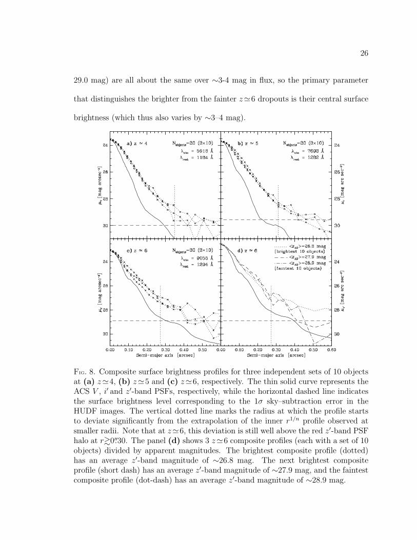
26

29.0 mag) are all about the same over ∼3-4 mag in flux, so the primary parameter

that distinguishes the brighter from the fainter z≃6 dropouts is their central surface

brightness (which thus also varies by ∼3–4 mag).

FIG. 8. Composite surface brightness profiles for three independent sets of 10 objectsat (a) z≃4, (b) z≃5 and (c) z≃6, respectively. The thin solid curve represents theACS V , i′ and z′-band PSFs, respectively, while the horizontal dashed line indicatesthe surface brightness level corresponding to the 1σ sky–subtraction error in theHUDF images. The vertical dotted line marks the radius at which the profile startsto deviate significantly from the extrapolation of the inner r1/n profile observed atsmaller radii. Note that at z≃6, this deviation is still well above the red z′-band PSFhalo at r&0′′.30. The panel (d) shows 3 z≃6 composite profiles (each with a set of 10objects) divided by apparent magnitudes. The brightest composite profile (dotted)has an average z′-band magnitude of ∼26.8 mag. The next brightest compositeprofile (short dash) has an average z′-band magnitude of ∼27.9 mag, and the faintestcomposite profile (dot-dash) has an average z′-band magnitude of ∼28.9 mag.

27

We used the IRAF3 procedure ELLIPSE to fit surface brightness profiles shown

in Figure 8 to each of the three independent composite images per redshift bin. We

also computed a mean surface-brightness profile from the three composite surface

brightness profiles generated from the three independent composite images for each

redshift bin. Figure 9 shows composite images for z≃4, 5, 6 objects. Here each com-

posite image is a stack of 30 objects. Figure 10 shows the average surface brightness

profiles for each of the redshift intervals z≃4, 5, 6. The thin solid curves in Figure 8

and the dot-dash curves in Figure 10 represent the observed ACS V , i′ and z′-band

Point Spread Functions (PSFs), while the horizontal dashed lines indicate the surface

brightness level corresponding to the 1σ sky–subtraction error in each of the HUDF

images. It is important to note that we scaled the ACS PSFs to match the surface

brightness of the central data point in our mean surface-brightness profile, to deter-

mine how extended the mean surface-brightness profile is with respect to the PSFs.

FIG. 9. Composite images for Left z≃4, Center z≃5 and Right z≃6 objects. Hereeach composite image is a stack of 30 objects. Each stamp is 1′′.53 on a side.

3IRAF (http://iraf.net) is distributed by the National Optical Astronomy Observatories, whichare operated by the Association of Universities for Research in Astronomy, Inc., under cooperativeagreement with the National Science Foundation.

28

(a) For z≃4 objects. (b) For z≃5 objects. (c) For z≃6 objects.

FIG. 10. Mean surface brightness profiles with a best fit Sersic profiles for 30 compositeimages at z≃4−6. The thin dot-dash curve represents the ACS V -, i′-, z′-band PSFs,respectively, while the horizontal dashed line indicates the surface brightness levelcorresponding to the 1σ sky–subtraction error in the HUDF images. The verticaldotted line marks the radius at which the profile starts to deviate significantly fromthe extrapolation of the inner r1/n profile observed at smaller radii. The n is the bestfit Sersic index.

In Figure 10, we fitted all possible combinations of the Sersic profiles (convolved

with the ACS PSF) to the observed profiles and using χ2 minimization, found the

best fits for galaxies at z≃ 4, 5, 6. The best fit Sersic index (n) for all three profiles

(z ≃ 4, 5, 6) is n < 2, meaning these galaxies follow mostly exponential disk-type

profiles in their central regions. We find that the observed profiles start to deviate

from the best-fit profiles at r &0′′.27, somewhat depending on the redshift. From

Figure 10, we also see that in each of V (z ≃ 4), i′ (z ≃ 5) and z′ (z ≃ 6), the PSF

declines more rapidly with radius than the composite radial surface brightness profile

for r &0′′.27. It is therefore unlikely that the observed ‘breaks’ result from the halos

and structure of the ACS PSFs. Specifically, at z≃6 the most significant deviations

in the light-profiles are seen at levels 1.5–2.0 mag above the 1σ sky-subtraction error,

and well above the PSF wings. Each of the mean surface brightness profiles display

29

a well-defined break, the radius of which appears to change somewhat with redshift.

These results are tabulated in Table 3. The vertical dotted lines (in Figure 8 and

Figure 10) mark the radius at which the mean surface brightness profiles start to

deviate significantly from the extrapolation of the r1/n profile observed at smaller

radii.

TABLE 3: Dynamical Ages for z≃4 − 6 Objects

Redshift “Break” Radiusa “Break” Radiusb Dynamical Agec

z (arcsec) (kpc) (τdyn)

4 0.35 2.5 0.09–0.29 Gyr5 0.31 2.0 0.07–0.21 Gyr6 0.27 1.6 0.05–0.15 Gyr

a From composite surface brightness profiles (Figure 8 and Figure 10).

b Radius in kpc corresponding to radius in arcsec at given redshift.

c If “break radius” interpreted as indicator of dynamical age.

Test of the stacking technique on nearby galaxies. — To test the general validity

of the stacking technique itself on a local galaxy sample, we used surface photometry

from the Nearby Field Galaxy Survey (NFGS: Jansen et al. 2000a,b). The NFGS

sample contains 196 nearby galaxies, that were objectively selected from the CfA

redshift catalog (CfA I; Davis & Peebles 1983; Huchra et al. 1983) to span the full

range in absolute B magnitude present in the CfA I (−14.7 .MB . −22.7 mag). The

absolute magnitude distribution in the NFGS sample approximates the local galaxy

luminosity function (e.g., Marzke et al. 1994), while the distribution over Hubble type

follows the changing mix of morphological types as a function of luminosity in the local

30

galaxy population. The NFGS sample (as detailed in Jansen et al. 2000a) minimizes

biases, and yields a sample that, with very few caveats, is representative of the local

galaxy population. As part of the NFGS, UBR surface photometry, both integrated

(global) and nuclear spectrophotometry, as well as internal kinematics were obtained

(see Jansen & Kannappan 2001). Here, we will concentrate on the U -band surface

photometry, since it is closest in wavelength to the rest-frame wavelengths observed at

z≃4−6. Although, ideally, we would want a filter further into the UV, Taylor-Mager

et al. (2007) and Windhorst et al. (2002) show that for the majority of late-type

nearby galaxies, the apparent structure of galaxies does not change dramatically once

one observes shortward of the Balmer break. Early-type galaxies, however, are a clear

exception to this, but these are not believed to dominate the galaxy population at

z≃4−6, as discussed before.

Figure 11 shows stacked profiles for relatively luminous early-, spiral-, and

late-type galaxies drawn from the NFGS. Vertical dotted lines indicate the half-light

radii and their intersection with the profiles, the surface brightness at that radius.

Dashed lines indicate exponential fits to the outer portion of each profile. Figure 11

also shows that co-adding profiles for disparate morphological types and for mid-type

spiral galaxies with a range in bulge-to-disk ratios can produce breaks in the composite

profile. No such breaks are seen when the profiles of either early-type galaxies (E,

S0) or late-type galaxies (Sd–Irr) are co-added. This figure shows that, if galaxies at

z≃4−6 had similar morphological types as local galaxies, then it would be possible

to produce a break in the profiles (as shown in Figure 8 and Figure 10), merely by

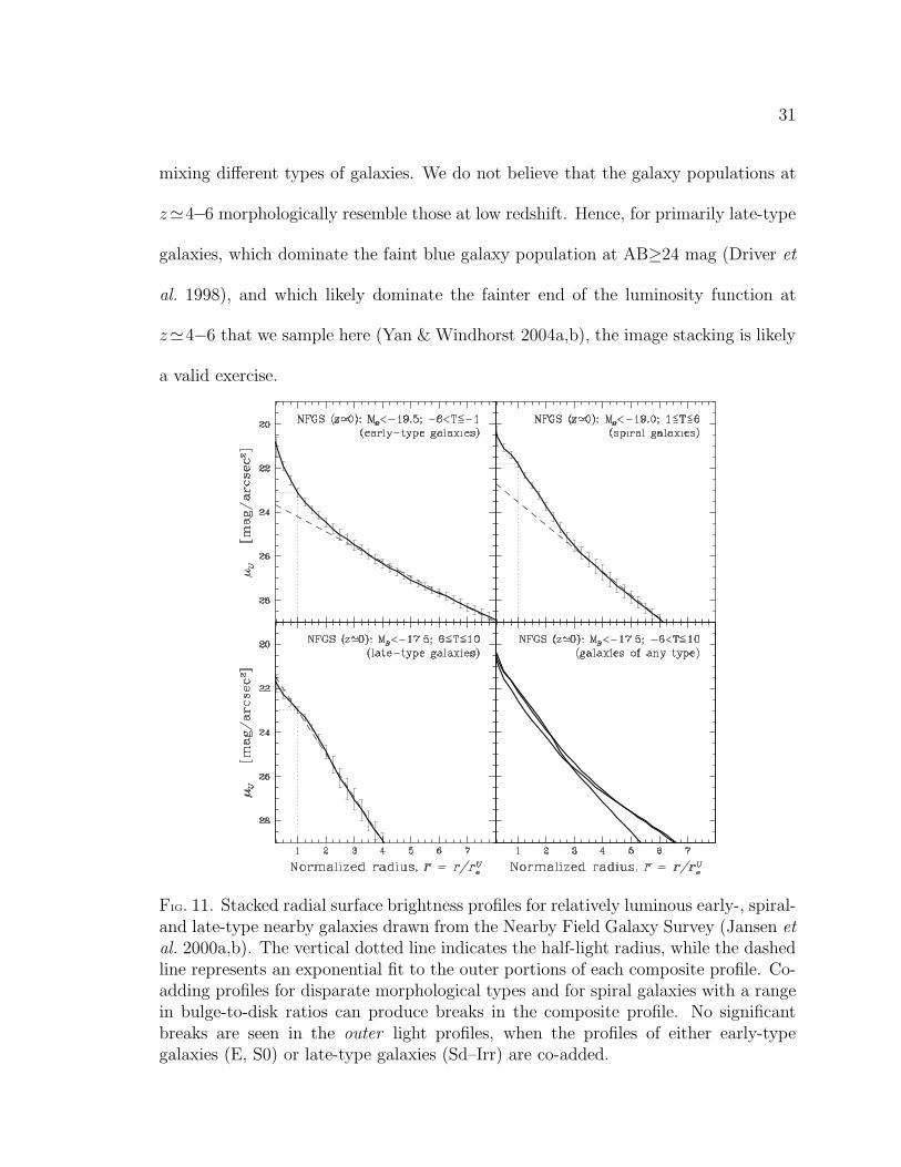
31

mixing different types of galaxies. We do not believe that the galaxy populations at

z≃4−6 morphologically resemble those at low redshift. Hence, for primarily late-type

galaxies, which dominate the faint blue galaxy population at AB≥24 mag (Driver et

al. 1998), and which likely dominate the fainter end of the luminosity function at

z≃4−6 that we sample here (Yan & Windhorst 2004a,b), the image stacking is likely

a valid exercise.

FIG. 11. Stacked radial surface brightness profiles for relatively luminous early-, spiral-and late-type nearby galaxies drawn from the Nearby Field Galaxy Survey (Jansen etal. 2000a,b). The vertical dotted line indicates the half-light radius, while the dashedline represents an exponential fit to the outer portions of each composite profile. Co-adding profiles for disparate morphological types and for spiral galaxies with a rangein bulge-to-disk ratios can produce breaks in the composite profile. No significantbreaks are seen in the outer light profiles, when the profiles of either early-typegalaxies (E, S0) or late-type galaxies (Sd–Irr) are co-added.

32

The primary goal of this section was to show that the profile stacking technique

is valid and can be used to get meaningful surface brightness profiles. We are not

comparing our nearby sample with galaxies at z ≃ 4−6. These nearby galaxies are

unlikely to be local analogues of high redshift galaxies. If we apply surface brightness

dimming to UV light-profiles of these nearby galaxies, they would be mostly invisible

to HST, and in some cases visible to the James Webb Space Telescope (JWST ; see

e.g., Windhorst et al. 2006). This is another way of saying that the z≃4−6 objects

are truly different from z≃0 objects.

2.6. Discussion

Figure 10 shows that the mean surface brightness profiles deviate significantly

from an inner r1/n profile at radii r&0′′.27–0′′.35, depending somewhat on the redshift

bin. These deviations appear real, with the break/point of departure located &1.5–

2 mag above the 1σ sky-subtraction error and above the PSF-wings. In the following,

we discuss several possible explanations for the observed shapes of our composite

surface brightness profiles.

Galaxies with different morphologies. — Our test on nearby galaxies (Fig-

ure 11) shows that, if we stack many galaxies with different morphologies (early-type,

late-type or spiral galaxies), it is possible to get a slope-change (‘break’) in the av-

erage surface brightness profile. Ravindranath et al. (2006) find that 40% of the

brighter LBGs at 2.5<z <5 have light profiles close to exponential, as seen for disk

galaxies, and only ∼30% have high n, as seen in nearby spheroids. They also find a

significant fraction (∼30%) of galaxies with light profiles shallower than exponential,

33

which appear to have multiple cores or disturbed morphologies, suggestive of close

pairs or on-going galaxy mergers. Therefore, if faint galaxies at z≃4−6 have a variety

of morphological types, then the shape of the average surface brightness profile that

we see may be due to the stacking of different types of galaxies. Therefore, we find

that the exponential and the flatter profiles found by Ravindranath et al. (2006) for

galaxies at 2.5<z<5 also apply to higher redshifts (z≥5).

Also, we believe that it is more likely that the high redshift, faint galaxy

population consists primarily of small galaxies with late-type morphologies and with

sub-L∗ luminosities, as seen at z≃2−3 (Driver et al. 1995, 1998). So if the z≃4−6

population consists of such a late-type galaxy population, then the slope-change in

the light profiles is likely not the result of co-adding images of objects with disparate

morphological types.

Central star formation/starburst. — HST optical images of galaxies at z≃4−6

sample their rest-frame UV (∼1200 A), where the contribution from the actively star-

forming regions (young, massive stars) dominates the UV-light. Hathi et al. (2008a)

have shown that galaxies at z≃5−6 are high redshift starbursts with similar starburst

intensity limit as local starbursting galaxies. Therefore, it is possible that galaxies at

z ≃ 4−6 have centrally concentrated star formation or starburst. This possibility is

based on three key assumptions: (1) most of the galaxies at z≃4, 5, 6 are intrinsically

later-type galaxies (Steidel et al. 1999); (2) the SED of these galaxies at z ≃ 4, 5, 6

are dominated by early A- to late O-type stars, respectively; and (3) there are no old

stars with ages at z≃4−6 greater than 2-1 Gyr in WMAP cosmology, respectively.

34

Hunter & Elmegreen (2006) studied azimuthally averaged surface photometry

profiles for large sample of nearby irregular galaxies. They find some galaxies have

double exponentials that are steeper (and bluer) in the inner parts compared to outer

parts of the galaxy. Hunter & Elmegreen (2006) discuss that this type of behavior

is expected in galaxies, where the centrally concentrated star formation or starburst

steepens the surface brightness profiles in the center. If that is the case, then one

might expect a better correlation between the break in the surface brightness profiles

and changes in color profiles. Unfortunately, for our sample of galaxies at z ≃ 4−6,

we don’t have high- resolution restframe UBV color information. The objects are

generally too faint for Spitzer Space Telescope, and hence we cannot confirm or reject

this possibility for the shape of our composite surface brightness profiles.

Limits to dynamical ages for z≃4, 5, 6 objects. — The average compact z≃4−6

galaxy is clearly extended with respect to the ACS PSFs (Figure 10), and is best fit

by an exponential profile (n < 2) out to a radius of about r ≃0′′.35, 0′′.31, and 0′′.27

at z≃4, 5 and 6, respectively. The apparent progression with redshift is noteworthy.

The radius at which the profile starts to deviate from r1/n (in this case at radius

r&0′′.35–0′′.27) may put an important constraint to the dynamical time scale of these

systems. If this argument is valid, then we can estimate limits to the dynamical ages

of z≃4, 5, 6 galaxies as follows.

In WMAP cosmology, a radius of r&0′′.35 at z≃ 4 corresponds to r&2.5 kpc.

The dynamical time scale (e.g., Binney & Tremaine 1987), τdyn, goes as τdyn =

Cr3/2/√

G M , where the constant C = π/2. For a typical dwarf galaxy mass range

35

of ∼ 109−108 M⊙ inside r=2.5 kpc, we infer that the limits to the dynamical age

would be τdyn ≃ 90–290 Myr, which is the lifespan expected for a late-type B-star.

This means that the last major merger that affected this surface brightness profile

and that triggered its associated starburst may have occurred ∼0.20 Gyr before z≃4,

—assuming that the star-formation was not spontaneous, but associated with some

accretion or a merging event.

Table 3 shows the break-radius and inferred limits to dynamical ages for the

z ≃ 4−6 objects. At z ≃ 5, we find that the limits to dynamical age at the break

radius would be τdyn ≃ 70–210 Myr, which is the lifespan expected for a mid B-star,

while at z≃6, τdyn ≃ 50–150 Myr, which is the lifespan expected for a late O–early

B-star. This means that the last major merger that affected these surface brightness

profiles at z≃5 and 6 and that triggered its associated starburst may have occurred

∼0.14 and ∼0.10 Gyr before z≃5 and 6, respectively.

The dynamical time is a lower limit to the actual time available, since it as-

sumes matter starts from rest. Any angular momentum at start will increase the

available time. The best-fit SED age from the GOODS HST and Spitzer photometry

on some of the brighter of these objects — using Bruzual & Charlot (2003) templates

— is in the range of about ∼150–650 Myr (Yan et al. 2005; Eyles et al. 2005, 2007),

the lower end of which is consistent with our limits to their dynamical age estimates,

while the somewhat larger SED ages could also be affected by the onset of the AGB

in the stellar population increasing the observed Spitzer fluxes and hence possibly

overestimating ages (Maraston 2005). Our age estimates for z≃ 4−6 are consistent

36

with the trend of SED ages suggested for z≃7 (Labbe et al. 2006). It is noteworthy

that, given the uncertainties, the two independent age estimates are consistent. If

our limits to dynamical age estimates for the image stacks are thus valid, they are

consistent with the SED ages, and point to a consistent young age for these objects.

Furthermore, the presence of young, massive late O–early B-stars at z≃6 has

implications for the reionization of the universe. From observations of the appearance

of complete Gunn-Peterson troughs in the spectra of z&5.8 quasars (Fan et al. 2006),

we know that the epoch of reionization had ended by z ≃ 6. From the steep (α=–

1.8) faint-end slope of the luminosity function of z ≃ 6 galaxies, Yan & Windhorst

(2004a,b) concluded that dwarf galaxies, and not quasars, likely finished reionization

by z ≃ 6. Should the present interpretation of their light profiles be correct, then

it would appear to add support to this picture, in the sense that such objects are

dominated by B-stars and did not start their most recent major starburst long before

z≃6. It is the same global starburst that would have finished reionization by z≃6.

2.7. Looking Towards the Future (JWST Science)

The results of this project are based on composite images of compact galaxies

in the HUDF at z ≃ 4−6. Composite images were generated to increase signal-to-

noise (S/N) ratio of faint individual galaxies. Such a composite would effectively

correspond to a single galaxy detectable at a much higher S/N ratio, equivalent to

∼4500 HST orbits (∼3000 hrs) on a single such object. It will be very difficult to

improve this analysis using the HST in next few years. The James Webb Space

Telescope (JWST ) will observe very distant galaxies (z&6) in the observed near-mid

37

infrared (IR) wavelengths after its launch in 2013. JWST will be very critical to

understand structure/morphologies of these faint galaxies at z & 4−6. JWST will

accomplish such a high S/N observations for faint galaxies at z≃4−6 in (1/12)th of

the time compared to current capabilities (see e.g., Windhorst et al. 2008). Therefore,

the 6.5 meter JWST will confirm and improve our results at 1 micron in 250 hours

of JWST deep imaging as a single object. JWST will also enable such analysis

on accuracy of sky background and composite images for galaxies at much higher

redshift (z≃7−15). We will be able to characterise JWST measured sky-background

and its uncertainties very carefully, as we have done in this project with the HUDF.

JWST ’s smaller pixel size, darker sky (due to its L2 orbit) and observed near to

mid-infrared wavelengths will help tremendously to make such a structural study for

very first galaxies around z≃10−15. It is very important to understand what type of

morphological structure these galaxies have, what the ages are of their first generation

of stars, how they formed, and how they contributed to the reionization process. It is

therefore critical that JWST be designed and built to allow to do ultra-deep near-mid

IR surveys. For the current purpose, this includes in particular that every reasonable

effort be maintained to keep the scattered light in this open-tubed telescope to a

minimum, so that we will be able to subtract the local JWST sky-background — on

.10 arcsec scales — to very high accuracy (.10−3 of the sky).

3. STARBURST INTENSITY LIMIT AT z≃5−6

3.1. Overview

The peak star formation intensity in starburst galaxies does not vary signifi-

cantly from the local universe to redshift z∼6. We arrive at this conclusion through

new surface brightness measurements of 47 starburst galaxies at z≃5−6, doubling the

redshift range for such observations. These galaxies are spectroscopically confirmed

in the Hubble Ultra Deep Field (HUDF) through the GRism ACS Program for Ex-

tragalactic Science (GRAPES) project. The starburst intensity limit for galaxies at

z≃5−6 agree with those at z≃3−4 and z≃0 to within a factor of a few, after cor-

recting for cosmological surface brightness dimming and for dust. The most natural

interpretation of this constancy over cosmic time is that the same physical mecha-

nisms limit starburst intensity at all redshifts up to z ≃ 6 (be they galactic winds,

gravitational instability, or something else). We do see two trends with redshift: First,

the UV spectral slope (β) of galaxies at z≃5−6 is bluer than that of z≃3 galaxies,

suggesting an increase in dust content over time. Second, the galaxy sizes from z≃3

to z≃6 scale approximately as the Hubble parameter H−1(z). Thus, galaxies at z≃6

are high redshift starbursts, much like their local analogs except for slightly bluer

colors, smaller physical sizes, and correspondingly lower overall luminosities. If we

now assume a constant maximum star formation intensity, the differences in observed

surface brightness between z ≃ 0 and z ≃ 6 are consistent with standard expanding

cosmology and strongly inconsistent with a tired light model.

3.2. Introduction

Star formation on galactic scales is a key ingredient in understanding galaxy

evolution. We cannot compare structure formation calculations to observed galaxy

39

populations without some model for how star formation proceeds. Such models are

based on detailed observations in the nearby universe, combined with physically moti-

vated scaling for differing conditions elsewhere in the universe. To test the validity of

such scaling, it is valuable to directly measure the properties of star formation events

in the distant universe, and see how they compare with their nearby counterparts.

Starbursts are regions of intense massive star formation that can dominate a

galaxy’s integrated spectrum. By comparing the properties of starbursts over a wide

range of redshifts, we can test whether the most intense star formation events look

the same throughout the observable history of the universe. High redshift galaxies

are expected, on average, to be less massive and lower in metal abundance than

their present-day counterparts. Either effect could in principle change the maximum

intensity of star formation that such galaxies can sustain.

Meurer et al. (1997, hereafter M97) measured the effective surface brightness,

i.e., the average surface brightness within an aperture that encompasses half of the

total light, for various samples. They conclude that the maximum effective surface

brightness of starburst galaxies is unchanged to better than an order of magnitude

out to redshifts z ≃ 3. Weedman et al. (1998, hereafter W98) measured observed

surface brightness from the single brightest pixel, and concluded that high-redshift

(2.2. z .3.5) starburst galaxies have intrinsic ultra-violet (UV) surface brightnesses

that are typically 4 times higher than for low-redshift starburst galaxies. Both M97

and W98 measured their surface brightness for spectroscopically confirmed galaxies

in the Hubble Deep Field (HDF; Williams et al. 1996).

40

We have measured the surface brightness of starburst regions at 3 . z . 6,

using photometry from the HUDF images (Beckwith et al. 2006) and redshifts from

the GRAPES project (Pirzkal et al. 2004). We combine these with earlier published

results comparing z ≃ 3 and z ≃ 0 starbursts (M97, W98). The starburst intensity

limit of starburst regions at 5.z.6 sample is consistent with that at z≃3 and z≃0

to within the uncertainties, which are about a factor of three. These high redshift star

forming regions are thus starbursts, with a star formation intensity similar to their

local counterparts, despite any effects of differing metallicity and/or galaxy size. The

starbursts should then be a set of standard surface brightness objects, and can be

used to apply Tolman’s test for expansion of the universe (Tolman 1930, 1934) over

an unprecedented redshift range (0<z.6). Our surface brightness observations fully

support standard expanding universe models. This result is robust to even rather

large systematic errors, thanks to the wide redshift range spanned by the data.

Throughout this chapter we denote the HST/Advanced Camera for Surveys

(ACS) F435W, F606W, F775W and F850LP filters as B, V , i′, z′, and HST/NIC3

F110W and F160W as J and H-bands, respectively. We assume a Wilkinson Mi-

crowave Anisotropy Probe (WMAP) cosmology of Ωm=0.24, ΩΛ=0.76 and H0=73

km s−1 Mpc−1 (Spergel et al. 2007). This implies an age for the Universe of 13.7 Gyr.

Magnitudes are given in the AB system (Oke & Gunn 1983).

3.3. Observations and Sample Selection

The HUDF is a 400 orbit survey of a 3.4′ × 3.4′ field carried out with the ACS

in the B, V , i′ and z′ filters (see Beckwith et al. 2006, for further details). We have

41

carried out deep unbiased slitless spectroscopy of this field with the ACS grism as part

of the GRAPES project, which was awarded 40 HST orbits during Cycle 12 (ID 9793;

PI S. Malhotra). The grism observations were taken at five different orientations in

order to minimize the contamination of the spectra by overlapping nearby sources.

We have extracted useful low resolution (R ≃ 100) spectra from 5900 A to 9500 A

for ∼1500 objects in the HUDF to a limiting magnitude of z′AB≃27.5 mag in the AB

system. Details of the observations, data reduction and final GRAPES catalog are

described in a paper by Pirzkal et al. (2004).

We identify high-redshift galaxies on the basis of their ACS grism spectra. This

identification was based on detecting the Lyman break in the continuum or the Lyα

emission for these sources. With the ACS grism low-resolution spectra, we are able

to determine the redshifts to an accuracy of ∆z≈0.15 even for the faintest detectable

Lyman-break galaxies (LBGs) (z′AB ≃27.5 mag). Details of the selection process are

described in Malhotra et al. (2005). There are 47 star-forming galaxies at z ≃ 5−6

in the GRAPES/HUDF with confirmed spectroscopic redshifts. These redshifts are

sufficiently high that the observed visible/red wavelengths measure the rest-frame UV

flux at wavelengths comparable to those at which M97 and W98 measured the surface

brightness of starburst regions at z . 3. We used the following spectroscopically

confirmed samples for our analysis.

• The z ≃ 3 LBGs from the Hubble Deep Field (HDF, Giavalisco et al. 1996;

Steidel et al. 1996a,b) were used to compare our measurements with M97. This

sample of 10 galaxies at z≃3 forms the subset of UV samples used by M97. We

42

measured the UV spectral slopes (β) using observed (V –I) and (G–R) colors,

and rest-frame UV fluxes were derived from the observed R-band (combined

V and I light) magnitudes (Giavalisco et al. 1996; Steidel et al. 1996a,b). Here

we denote the HST/WFPC2 F606W and F814W filters as V and I-bands,

respectively. The G and R filters are defined in Steidel & Hamilton (1993).

• The z≃4 B-band dropout galaxies were selected from the VLT redshift catalog

of Vanzella et al. (2006). This sample is small (4 galaxies), but is useful for

comparing z≃3−4 and z≃5−6 galaxy samples. We used the observed (i′–z′)

color to estimate β, and rest-frame UV fluxes were derived from the observed

z′-band magnitudes. The observed i′- and z′-band magnitudes for z≃4 galaxies

were obtained from the HUDF/GOODS catalogs of Beckwith et al. (2006).

• We use a sample of 47 z ≃ 5−6 starburst galaxies having GRAPES redshifts

(Malhotra et al. 2005; Rhoads et al. 2008) in the HUDF. Table 4 shows prop-

erties (coordinates, magnitudes, sizes and redshifts) for these 47 galaxies. We

have only 19 galaxies (out of 47) covered by the Thompson et al. (2005) HUDF

NICMOS images and therefore with J and H magnitudes. We estimate β from

the observed (J–H) color. The rest-frame UV fluxes were derived from the

observed J and H-band magnitudes for 19 galaxies, while the average β is used

to predict J and H-band magnitudes for the remaining 28 galaxies for which we

did not have NICMOS coverage.

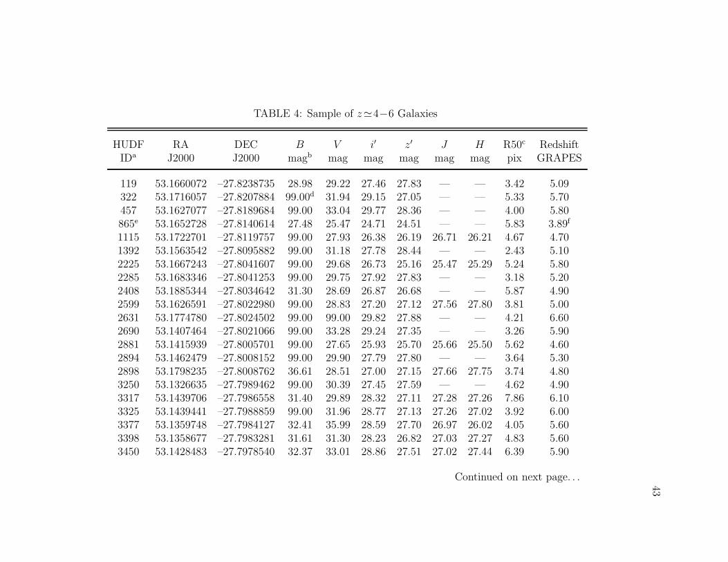
43

TABLE 4: Sample of z≃4−6 Galaxies

HUDF RA DEC B V i′ z′ J H R50c RedshiftIDa J2000 J2000 magb mag mag mag mag mag pix GRAPES

119 53.1660072 –27.8238735 28.98 29.22 27.46 27.83 — — 3.42 5.09322 53.1716057 –27.8207884 99.00d 31.94 29.15 27.05 — — 5.33 5.70457 53.1627077 –27.8189684 99.00 33.04 29.77 28.36 — — 4.00 5.80865e 53.1652728 –27.8140614 27.48 25.47 24.71 24.51 — — 5.83 3.89f

1115 53.1722701 –27.8119757 99.00 27.93 26.38 26.19 26.71 26.21 4.67 4.701392 53.1563542 –27.8095882 99.00 31.18 27.78 28.44 — — 2.43 5.102225 53.1667243 –27.8041607 99.00 29.68 26.73 25.16 25.47 25.29 5.24 5.802285 53.1683346 –27.8041253 99.00 29.75 27.92 27.83 — — 3.18 5.202408 53.1885344 –27.8034642 31.30 28.69 26.87 26.68 — — 5.87 4.902599 53.1626591 –27.8022980 99.00 28.83 27.20 27.12 27.56 27.80 3.81 5.002631 53.1774780 –27.8024502 99.00 99.00 29.82 27.88 — — 4.21 6.602690 53.1407464 –27.8021066 99.00 33.28 29.24 27.35 — — 3.26 5.902881 53.1415939 –27.8005701 99.00 27.65 25.93 25.70 25.66 25.50 5.62 4.602894 53.1462479 –27.8008152 99.00 29.90 27.79 27.80 — — 3.64 5.302898 53.1798235 –27.8008762 36.61 28.51 27.00 27.15 27.66 27.75 3.74 4.803250 53.1326635 –27.7989462 99.00 30.39 27.45 27.59 — — 4.62 4.903317 53.1439706 –27.7986558 31.40 29.89 28.32 27.11 27.28 27.26 7.86 6.103325 53.1439441 –27.7988859 99.00 31.96 28.77 27.13 27.26 27.02 3.92 6.003377 53.1359748 –27.7984127 32.41 35.99 28.59 27.70 26.97 26.02 4.05 5.603398 53.1358677 –27.7983281 31.61 31.30 28.23 26.82 27.03 27.27 4.83 5.603450 53.1428483 –27.7978540 32.37 33.01 28.86 27.51 27.02 27.44 6.39 5.90

Continued on next page. . .

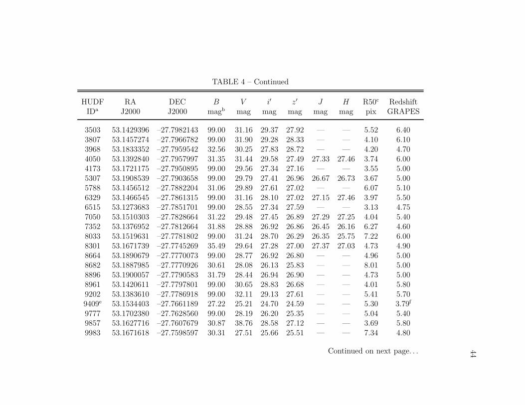
44

TABLE 4 – Continued

HUDF RA DEC B V i′ z′ J H R50c RedshiftIDa J2000 J2000 magb mag mag mag mag mag pix GRAPES

3503 53.1429396 –27.7982143 99.00 31.16 29.37 27.92 — — 5.52 6.403807 53.1457274 –27.7966782 99.00 31.90 29.28 28.33 — — 4.10 6.103968 53.1833352 –27.7959542 32.56 30.25 27.83 28.72 — — 4.20 4.704050 53.1392840 –27.7957997 31.35 31.44 29.58 27.49 27.33 27.46 3.74 6.004173 53.1721175 –27.7950895 99.00 29.56 27.34 27.16 — — 3.55 5.005307 53.1908539 –27.7903658 99.00 29.79 27.41 26.96 26.67 26.73 3.67 5.005788 53.1456512 –27.7882204 31.06 29.89 27.61 27.02 — — 6.07 5.106329 53.1466545 –27.7861315 99.00 31.16 28.10 27.02 27.15 27.46 3.97 5.506515 53.1273683 –27.7851701 99.00 28.55 27.34 27.59 — — 3.13 4.757050 53.1510303 –27.7828664 31.22 29.48 27.45 26.89 27.29 27.25 4.04 5.407352 53.1376952 –27.7812664 31.88 28.88 26.92 26.86 26.45 26.16 6.27 4.608033 53.1519631 –27.7781802 99.00 31.24 28.70 26.29 26.35 25.75 7.22 6.008301 53.1671739 –27.7745269 35.49 29.64 27.28 27.00 27.37 27.03 4.73 4.908664 53.1890679 –27.7770073 99.00 28.77 26.92 26.80 — — 4.96 5.008682 53.1887985 –27.7770926 30.61 28.08 26.13 25.83 — — 8.01 5.008896 53.1900057 –27.7790583 31.79 28.44 26.94 26.90 — — 4.73 5.008961 53.1420611 –27.7797801 99.00 30.65 28.83 26.68 — — 4.01 5.809202 53.1383610 –27.7786918 99.00 32.11 29.13 27.61 — — 5.41 5.709409e 53.1534403 –27.7661189 27.22 25.21 24.70 24.59 — — 5.30 3.79f

9777 53.1702380 –27.7628560 99.00 28.19 26.20 25.35 — — 5.04 5.409857 53.1627716 –27.7607679 30.87 38.76 28.58 27.12 — — 3.69 5.809983 53.1671618 –27.7598597 30.31 27.51 25.66 25.51 — — 7.34 4.80

Continued on next page. . .

45

TABLE 4 – Continued

HUDF RA DEC B V i′ z′ J H R50c RedshiftIDa J2000 J2000 magb mag mag mag mag mag pix GRAPES

20191 53.1725568 –27.8137124 31.23 27.15 25.77 25.67 25.81 25.51 5.79 4.6730591 53.1553196 –27.8151593 33.39 31.37 32.27 27.51 — — 4.99 6.7032042 53.1689736 –27.8007244 99.00 32.72 31.75 28.84 — — 4.00 5.7533003 53.1460653 –27.7944931 99.00 99.00 31.63 28.00 27.47 27.35 4.01 6.4035506 53.1660816 –27.7719653 30.31 32.92 31.06 27.82 — — 5.97 6.2036383 53.1677041 –27.7681044 99.00 99.00 31.07 28.66 — — 5.58 5.80–101e 53.1770656 –27.7643556 26.23 24.52 24.20 24.22 — — 7.50 3.60f

–102e 53.1431467 –27.8155017 27.95 25.10 24.17 24.14 — — 9.70 4.14f

a Identification from the HUDF catalogs of Beckwith et al. (2006),ACS grism spectra from Malhotra et al. (2005).

b All Magnitudes are given in the AB system.

c Half light radius (R50) measured in z′-band.

d A magnitude of 99.00 indicates no detection.

e Objects from Beckwith et al. (2006) B-band dropout catalog.Two objects with negative IDs don’t have published HUDF IDs.

f Redshifts from Vanzella et al. (2006).

46

3.4. Starburst Intensity Limit (M97 Approach)

Magnitudes and color measurements. — All measurements for galaxies at

z ≃ 4−6 were done on the HST/ACS HUDF images (Beckwith et al. 2006) and

HST/NICMOS images (Thompson et al. 2005). The HST/NICMOS images were

reprocessed by L. Eddie Bergeron (private communication). The HST/NICMOS

images cover ∼50% of the HUDF ACS field. Therefore, only half of our galaxies

have J- and H-band imaging. We need J and H magnitudes for galaxies at z≃5−6

to measure the UV spectral slopes and luminosities at ∼2200 A rest-frame. We use

rest-frame ∼2200 A to measure the effective surface brightness for consistency with

M97. All broad-band magnitudes are measured as SExtractor (Bertin & Arnouts

1996) MAG AUTO magnitudes, using dual-image mode to generate aperture-matched

catalogs. We use the z′-band image as the detection image. MAG AUTO apertures are

Kron-like (Kron 1980) flexible apertures, which enclose most of the flux for an object.

These apertures are same in all the filters for a given object. We also measured

SExtractor Petrosian (1976) magnitudes (MAG PETRO), with η=0.2 (Holwerda 2005),

and isophotal magnitudes (MAG ISO). We find that the average difference between

MAG AUTO and MAG PETRO is ∼0.1 mag (i.e., 〈mauto−mpetro〉 = ±0.1), while the average

difference between MAG AUTO and MAG ISO is ∼0.2 mag (i.e., 〈mauto − miso〉 = ±0.2).

The effect of this magnitude uncertainty on the surface brightness measurements

is very small (<0.1 dex). Our method to measure magnitudes is the same for all

galaxies at z≃4−6, and is consistent with the curve-of-growth method used for our

comparison sample of z ≃ 3 galaxies (Giavalisco et al. 1996; Steidel et al. 1996a,b).

47

We use MAG AUTO magnitudes to calculate the UV spectral slope (β) and the effective

surface brightness.

The UV spectral slope (β). — The UV spectral slope (β) is determined from

a power-law fit to the UV continuum spectrum (Calzetti et al. 1994),

fλ ∝ λβ ,

where fλ is the flux density per unit wavelength (ergs s−1 cm−2 A−1). Converting

this into magnitude units yields a linear relationship between β and colors. Figure 12

shows the average values of the UV spectral slopes, β, for galaxies at z ≃ 3−4 and

z≃5−6. The mean values are plotted with error bars indicating the standard deviation

of the mean (i.e., the sample standard deviation (σ) divided by the square root of

the sample size (N)). The UV slopes for 10 galaxies at z≃3 are obtained using the

following two equations (M97) for two slightly different samples:

β = 2.55 · (G − R) − 2 and β = 3.23 · (V − I) − 2 .

Here G and R filters are defined in Steidel & Hamilton (1993). We also plot the

average β measured for 4 galaxies at z≃4, using:

β = 5.65 · (i′ − z′) − 2

where we have used pivot wavelengths for i′- and z′-band, λi=7693 A and λz′=9055 A,

respectively, to obtain the slope of 5.65 in the β–color linear relationship. Figure 12

also shows the average β for 19 galaxies at z≃5−6 obtained using

β = 2.56 · (J − H) − 2

48

where pivot wavelengths for the J- and H-bands are λJ=11200 A and λH=16040 A,

respectively, to obtain the slope of 2.56 in β–color relationship. We do not use (z′–J)

color to estimate β for galaxies at z≃5−6, because the (z′–J) colors can be insensitive

to rest-frame UV colors due to the shorter color baseline, and are also more sensitive

to uncertainties in the optical to infrared zero points (Bouwens et al. 2006). Therefore

for comparison, we also measured β for galaxies at z≃5 using (i′–z′) colors and found

that the average β is –1.53±0.38 compared to –1.65±0.21, the average β at z≃5 using

(J–H) colors. This implies that small variations in the UV rest-frame wavelength and

observed colors do not affect the slope within the quoted uncertainties.

FIG. 12. UV spectral slopes (β)vs. redshift relation. Mean βare plotted with error bars indi-cating the standard deviation ofthe mean (i.e., σ/

√N). We have

plotted the data points at z ≃ 3from Adelberger & Steidel (2000)and at z ≃ 6 from Bouwens et al.(2006) for comparison.

Figure 12 shows that the average β decreases from –1.13±0.17 at z ≃ 3 to

–1.74±0.35 at z ≃ 6. The change in the average slope shows that the galaxies at

z≃5−6 are bluer than those at z≃3, but still somewhat redder than the flat slope

in fν (fλ ∝ λ−2), that would be expected for a dust-free starburst galaxy.

49

Half-light radius (re or R50) measurements. — The half-light radius is defined

as the radius containing 50% of the total flux of an object. The half-light radii for

galaxies at z≃3 are derived by Giavalisco et al. (1996) & Steidel et al. (1996b) and

are measured such that half of the total emission from the starburst is enclosed within

a circular aperture. We used the SExtractor half-light radii (R50, radii enclosing

50% of the flux within a circular aperture) obtained from the HUDF z′-band catalog

(Beckwith et al. 2006) for galaxies at z≃4−6. All radii are converted from arcsecs to

kpc using a WMAP cosmology in the cosmological calculator by Wright (2006). The

half-light radii for galaxies at z ≃ 4−6 are measured at rest-frame UV wavelengths

λ=1500±300 A. The sizes do not change appreciably when measured within this

wavelength range. Figure 13 shows the average values of the half-light radii for 10

starburst galaxies at z≃3, 4 starburst galaxies at z≃4, and 47 starburst galaxies at

z ≃ 5−6. Mean half-light radii are plotted with error bars indicating the standard

deviation of the mean. The solid and dashed curves show the trend if sizes evolve

as H−1(z) or H−2/3(z), respectively, where H(z) is the Hubble parameter at redshift

z. The curves are normalized to the mean size we measure at z≃ 4 (∼0′′.21 or ∼1.5

kpc). Comparison between galaxies at z≃3 and z≃5−6 shows that the galaxy sizes

increase as we go from z≃6 to z≃3.

We independently measured various flavors of SExtractor radii (half-light,

Petrosian (1976), Kron) for galaxies at z ≃ 5−6 to assess the differences in these

measurements. The Petrosian radius is defined as the radius at which the surface

brightness is certain factor (η) of the average surface brightness within this isophote,

50

FIG. 13. Size (half-light radii) andredshift relation. Mean half-lightradii are plotted with error barsindicating the standard deviationof the mean (i.e., σ/

√N). The

solid and dashed curves shows thetrend if sizes evolve as H−1(z)and H−2/3(z), respectively. Bothcurves are normalized to the meansize at z≃4 (∼0′′.21 or ∼1.5 kpc).We have plotted the data points atz ≃ 3 from Ferguson et al. (2004)and at z ≃ 6 from Bouwens et al.(2006) for comparison.

while the Kron radius is defined as the typical size of the flexible aperture computed

from the moments (see SExtractor manual by Holwerda 2005, for further details).

The average difference between the half-light and the other two radii was approxi-

mately ±0′′.04. Therefore, we expect about 30% uncertainty in the measurements of

the half-light radii for galaxies at z≃5−6.

Calculation of surface brightness for starburst galaxies. — We measure the ef-

fective surface brightness for 14 starburst galaxies at z≃3−4 and 47 starburst galaxies

at z ≃ 5−6 by adopting the method used by M97. First, we need to estimate dust

extinction A1600 and k-corrections from the UV spectral slope (β). Dust extinction

is estimated using the linear empirical relation between A1600 and β (Meurer et al.

1999), which is given by following equation:

A1600 = 4.43 + 1.99 · (β)

where A1600 is the net absorption in magnitudes by dust at 1600 A.

51

The next step in correcting apparent flux for corresponding rest-frame UV

flux is to apply, where appropriate, the k-correction. We use following equation to

estimate k-correction (M97):

k =f2320

fλc/1+z

=

[

(1 + z) · 2320 A

λc

]β

where λc corresponds to the central wavelength of the filters used for the observed flux.

Here, we reference all observations to the observations in M97, which use a UV central

wavelength of 2320 A. We apply above mentioned dust and k-corrections to apparent

magnitudes to estimate absolute magnitudes and intrinsic UV luminosities for our

samples of z≃3−6 galaxies. The ratio of intrinsic UV to bolometric luminosity can

be calculated for young starbursts. By using the stellar population models of Bruzual

& Charlot (2003) to convert from intrinsic F220W flux/luminosity to bolometric

luminosity, we find that the ratio of the UV to bolometric luminosity changes due

to variations in the metallicity and the dust attenuation. The luminosity ratio spans

a range from ∼0.2 to ∼0.5. The adopted ratio of the intrinsic UV to bolometric

luminosity is:

L

Lbol

≃ 0.33

We are using this value for the UV to bolometric luminosity ratio for two reasons:

(1) this bolometric correction is very close to the average value we get from our stellar

population models, and

(2) this correction factor is also predicted by the models used by M97.

52

From Lbol and the half-light radii (re), we calculate effective surface brightness

(Se) using following relation:

Se =Lbol

2πr2e

(

L⊙

kpc2

)

.

Here re is measured in kpc and Lbol in solar luminosities (L⊙).

To characterize the Se distribution for all galaxies in our sample we consider

the median and 90th percentiles, which we denote as Se,50 and Se,90, respectively. The

upper limit to the surface brightness (starburst intensity limit) of starbursts is traced

by Se,90. Here we have used average β (from Figure 12) for each sample to estimate

the surface brightness. Figure 14 shows Lbol and Se as a function of re for the z≃0−6

galaxy samples. The z≃0 and z≃0.4 surface brightness measurements are taken from

M97. The z≃0 data point is the median measurement for 11 nearby galaxies (M97).

The Se,50 and Se,90 surface brightness levels of the combined sample are plotted as

dashed and dotted lines respectively.

The top panel of the Figure 14 shows that the bolometric luminosities for

galaxies at z ≃ 5−6 are smaller than the luminosities of galaxies at z ≃ 3. Using a

two-sided K-S test on these luminosity distributions, we reject the hypothesis that

the z ≃ 3 and z ≃ 5−6 luminosities are drawn from the same population at >99%

probability. From the bottom panel of Figure 14, it is apparent that Se shows little

or no dependence on re over about one order of magnitude in size; hence there is no

dependence on Lbol over about two orders of magnitude in luminosity. Figure 15 shows

the effective surface brightness (Se) as a function of redshift. The z ≃ 0 and z ≃ 0.4

surface brightness measurements are taken from M97. From Figure 14 and Figure 15,

53

FIG. 14. Bolometric luminosity (Lbol⊙

) andeffective surface brightness (Lbol

⊙kpc−2)

against effective radii for starburst galax-ies. The filled squares, circles and trian-gles are measurements for galaxies at z≃3,z≃4 and z≃5−6, respectively. The opensquare (z≃0) is the median measurementof 11 nearby galaxies from M97. The openhexagons (z ≃ 0.4) are Se measurementsfrom M97. The dotted and dashed linescorrespond to Se,90 and Se,50 of the com-bine sample. Uncertainties in z≃3−6 sur-face brightness and radii measurements areshown in lower right corner.

Log (Re [pc])

we find that Se,90 of the starbursts remains constant (within the uncertainties) with

redshift over the redshift range z≃0−6.

3.5. Starburst Intensity Limit (W98 Approach)

We also studied the surface brightnesses using the brightest pixel approach

pioneered by Weedman et al. (1998). Weedman et al. (1998) measures observed

surface brightness of the brightest pixel for galaxies at 2.2.z .3.5 in the HDF and

compared with the local starbursts by fading their observed (fλ) surface brightness

by (1+z)−5. We use this approach to compare surface brightnesses of the brightest

pixel for galaxies at z ≃3−6.

A postage stamp (51×51 pixels) for each galaxy at z ≃ 5−6 was excised

from the z′-band HUDF image. Using z′-band segmentation maps, only object pixels

were selected. For each object pixel in the postage stamp, we estimate the apparent

54

FIG. 15. Bolometric effective surfacebrightness (Lbol

⊙kpc−2) as a function of

redshift. The open square (z ≃ 0) isthe median measurement of 11 nearbygalaxies from M97. The filled squares(z ≃ 0.4) are Se measurements fromM97. The filled squares (z ≃ 3) arethe galaxies from the sample of M97for which we measured surface bright-nesses. The circles are the galaxies inour sample (z≃4−6). The dotted anddashed lines correspond to Se,90 andSe,50 of the combined sample. Uncer-tainties in z ≃ 3−6 surface brightness(due to radii and flux uncertainties) isshown in lower left corner.

magnitude. For the brightest pixel in each galaxy, the average UV spectral slope β

was used to predict J-band (for galaxies at z≃5) and H-band (for galaxies at z≃6)

magnitudes from z′-band apparent magnitudes. Using similar approach as discussed

in previous chapter, we calculated the intrinsic UV luminosity (LUV⊙

) for the brightest

pixel in each galaxy at z≃5−6. For surface brightness measurements, we divide the

intrinsic UV luminosity by the area of one pixel in kpc2.

Figure 16 shows surface brightness (LUV⊙

kpc−2) for the brightest pixel in each

of the 47 galaxies at z≃5−6 and 4 galaxies at z≃4. We have also plotted 18 galaxies at

z≃3 from W98. The W98 galaxies has observed surface brightnesses for the brightest

pixels and hence, for proper comparison, we converted observed surface brightnesses

for W98 galaxies to their corresponding rest-frame surface brightnesses. Here we have

used average β for z ≃ 3 galaxies as shown in Figure 12, to estimate extinction and

k-correction. The median (Sbp,50) and 90th percentile (Sbp,90) surface brightness levels

55

of the combined sample are plotted as dashed and dotted lines, respectively. Here,

the starburst intensity limit of starbursts is traced by Sbp,90. The Sbp,90 of galaxies at

z≃3 and z≃5−6 is same to within a factor of ∼0.10 dex.

FIG. 16. Surface Brightness obtainedfrom the brightest pixel of 47 galaxyimages at z≃5−6 and 4 galaxy imagesat z ≃ 4 . The squares are 18 W98galaxies. The W98 galaxies had ob-served surface brightnesses and hence,for proper comparison, we convertedobserved surface brightnesses to cor-responding rest-frame surface bright-nesses. The dotted and dashed linescorrespond to Sbp,90 and Sbp,50 of thecombine sample. Uncertainties in sur-face brightness (due to flux uncertain-ties) is shown in lower right corner.

We cannot properly compare the brightest pixel surface brightnesses between

the W98 sample at z≃0 and galaxies at z≃3−6 for two reasons. First, the aperture

sizes for W98 galaxies at z ≃ 0 are larger than the physical sizes corresponding to

one pixel at z ≃ 3−6, and the sizes for W98 galaxies at z ≃ 0 are also larger than

the effective radii measured by Meurer et al. (1995) for some of these local galaxies.

Second, the discrepancy between the W98 adopted UV spectral slope (β) and β from

Meurer et al. (1995) is large for some of these galaxies, which affects the applied

extinction for their luminosity measurements.

Our analysis of the effective surface brightness (Se) approach of M97 and the

brightest pixel (Sbp) approach of W98 suggests that the starburst intensity limit, as

56

defined by Se,90 or Sbp,90, of the starbursts is unchanged (within uncertainties) from

z≃5−6 to z≃3.

3.6. Results and Discussion

Selection and measurement effects. — In following section, we discuss esti-

mated uncertainties in the starburst intensity limit due to selection and measurement

effects:

Different radii-measurements: The results shown in Figures 13, 14 and 15 use

SExtractor half-light radii derived by Beckwith et al. (2006). Here we discuss the

uncertainty in the surface brightness measurements due to radii measurements. We

use three different flavors of radii measured using SExtractor. We measured the

half-light radii, the Petrosian (1976) radii and the Kron radii for galaxies at z≃5−6.

We found that the average difference between the half-light radius and other two

radii was approximately ±0′′.04. This difference does not affect our conclusion that

z≃5−6 galaxies are smaller compared to z≃3 galaxies. As shown in Figure 13, the

average value of the half-light radii for galaxies at z≃5−6 is 0′′.14 compared to 0′′.32,

which is the average value for galaxies at z ≃ 3. The uncertainty in three different

radii measurements is ±0′′.04. Therefore for a given luminosity, we expect that this

difference in radii measurement will cause ∼0.2 dex difference in Se,90 estimate.

Surface brightness selection: The limiting surface brightness in the HUDF

samples is Se ∼ 5.0 x 109 L⊙ kpc−2 at z ≃ 5−6, which is much fainter than the

observed maximum surface brightness (Se,90 ≃ 2.3 x 1011 L⊙ kpc−2) for all galaxies.

57

At the low surface brightness limit, our sample could be incomplete, but at the

maximum surface brightness level our sample is complete.

Size selection effect: The z≃3 galaxies are spectroscopically confirmed by Keck

observations. The limiting magnitude for Keck spectroscopy is R . 25.3 (Steidel et al.

1996b). Using Se,90 and the limiting magnitude, we estimate the minimum observable

size for this sample as ∼700 pc or ∼0′′.1. Therefore, this sample of galaxies at z≃3 is

not biased against smaller sizes.

Flux uncertainty: Here we discuss three possible sources of uncertainties in the

magnitudes (for a given size) that will affect our surface brightness measurements.

They are as follows: (1) The average SExtractor uncertainties in J and H magnitudes

are ∼0.2 mag. The largest magnitude uncertainties in the sample range up to ∼0.5

mag for three objects. Even this worst case magnitude uncertainty affects Se,90 by

only ∼0.2 dex. The uncertainty in Se,90 due to the average difference between various

magnitudes (MAG AUTO, MAG PETRO and MAG ISO) is very small (<0.1 dex) and hence

the uncertainties in J , H magnitudes dominate the uncertainty in Se,90. (2) The

ratio of the UV to bolometric luminosity for starburst galaxies is based on the stellar

population models. We find that this ratio is affected by the change in metallicity or

dust extinction in the stellar population models. The uncertainty in this ratio can

be as large as a factor of ∼2.0. This uncertainty in the bolometric correction will

change Se,90 estimate by ∼0.3 dex but this is systematic uncertainty and will affect

all starburst galaxies. (3) We have used linear fit to the observed relation between

the FFIR/F1600 and the UV spectral slope (β) to estimate A1600 (Fig.1 in Meurer et

58

al. 1999). The scatter in this plot can cause an uncertainty in A1600 of ∼0.4 mag.

This uncertainty in A1600 will change Se,90 estimate by ∼0.2 dex. This uncertainty

will systematically affect all galaxies in this study.

Therefore, if these logarithmic uncertainties add in quadrature, we would ex-

pect the total uncertainty in Se,90 to be ∼0.5 dex.

The starburst intensity limit. — We measure the effective surface brightness

(Se) and the brightest pixel surface brightness (Sbp) of the spectroscopically confirmed

galaxies at z≃5−6 in the HUDF and compare with the spectroscopically confirmed

galaxies at z ≃ 3 in the HDF. We conclude that to better than a factor of 3, the

starburst intensity limit of starbursts at z≃3 and z≃5−6 are the same. Using the K-S

test on these distributions, the resulting probabilities (&20%) support the hypothesis

that these distributions are drawn from the same population. By combining the

samples at z ≃ 3−4 and z ≃ 5−6, we find a mean Se,90 ≃ 2.3 x 1011 L⊙ kpc−2

(with a factor of 3 or ∼0.5 dex uncertainty). We quantify the scatter in the Se and

Sbp distributions (Figures 15 and 16) by measuring standard deviation (σ) from a

Gaussian fit to these distributions. We find that the scatter in the Se distribution

(σlog(Se) ≃ 0.37) is higher than the scatter in the Sbp distribution (σlog(Sbp) ≃ 0.27).

Therefore, the brightest pixel method could be very useful in estimating the starburst

intensity limit of starburst galaxies.

The approximate constancy of peak starburst intensity can be interpreted as

the evidence that the interstellar medium (ISM) can only support some maximum

pressure. Heckman et al. (1990) used [S II] emission line ratios to determine the

59

ISM pressure (P0) for a sample of galaxies (mostly starbursts) undergoing a strong

galactic wind. The star formation intensity required to produce P0 is Se ≃ 1.7 x 1011

L⊙ kpc−2 (M97). This value agrees closely with our Se,90, but was derived using

different method. The physical process can be explained by assuming that the ISM

pressure provides a “thermostat” for star-formation, such that strong outflows will

result whenever the pressure rises above P0 and shut down further star formation for

a time. This results in a characteristic peak starburst intensity. We convert Se,90 to

an equivalent star formation intensity (M⊙ yr−1 kpc−2) by using conversion factors

between UV luminosity and star-formation rate from Kennicutt (1998) and M97. We

get a star-formation intensity in the range of 30–50 M⊙ yr−1 kpc−2, depending on

the conversion factor. This peak intensity is physically distinct from the minimum

intensity required to produce a galactic wind, which is orders of magnitude lower, at

∼ 0.1 M⊙ yr−1 kpc−2 (Lehnert & Heckman 1996; Heckman 2001). Thus, every galaxy

in our sample is expected to have a galactic wind, as Lehnert et al. (2007) remark for

a similar sample of z&3 LBGs. However, only in galaxies near the starburst intensity

limit does the “thermostat” become active.

While the peak starburst intensity stays constant with redshift, the dust optical

depth that we infer from the observed spectral slope β decreases systematically with

redshift. This suggests that the star formation intensity limit does not depend on

dust content, at least over the range of dust optical depths τdust & 1 probed by

our sample. At yet higher redshifts we might expect that τdust < 1, and that the

starburst radiation field would no longer couple efficiently to the interstellar medium.

60

Whether this would substantially change the starburst intensity limit would depend

on the fraction of starburst wind driving that is due to radiation pressure, rather than

stellar winds and mechanical energy from supernova explosions.

The constancy of maximum star-formation surface intensity with redshift pro-

vides a basis for a strong test of the expanding Universe. Standard cosmologies predict

that the bolometric surface brightness should vary with redshift as (1 + z)−4. Our

results (using standard cosmology) combined with M97 results at low redshifts show

that the maximum star formation intensity remains constant (within uncertainties)

from z ≃ 0 to z ≃ 6. This conclusion depends critically on the use of a standard

cosmology to go from observed flux and radius to inferred star formation intensity.

Thus, if the peak star formation rate per unit area is controlled by some physical

limit that is based on local, redshift-independent physics, our observations essentially

require standard surface brightness dimming. While other evolutionary effects could

become important, we have minimized these by measuring surface brightnesses at

nearly fixed rest wavelength. Had we instead taken a “tired light” model, where

bolometric surface brightness falls of as (1+ z)−1, our observations would require the

true star formation intensity to be dramatically lower at high redshift— by a factor of

order (1 + z)3 ∼ 73 ∼ 300. This factor greatly exceeds the estimated uncertainties in

our analysis. Hence, the wide redshift range of our sample yields a strong application

of Tolman’s test (Tolman 1930, 1934), and we derive strong evidence in favor of the

expanding Universe and against any alternative “tired light” models.

61

Size and luminosity evolution. — An average galaxy at z≃5−6 in our sample

has half-light radii of ∼0.8 kpc or ∼0′′.14, as shown in Figure 13, which is in good

agreement with a number of recent studies (Bouwens et al. 2004b, 2006; Pirzkal et al.

2007; Dow-Hygelund et al. 2007). Ferguson et al. (2004) compares sizes of galaxies at

z≃1–5 within a fixed luminosity range. Our results agree with Ferguson et al. (2004)

for z≃3−4. The UV intrinsic luminosities for our sample of galaxies are brighter or

equal to L∗ (i.e., L&L∗) at respective redshifts, but we do not require any particular

minimum luminosity, while Ferguson et al. (2004) do require a minimum luminosity.

Given that the maximum surface brightness is near-constant, a minimum luminosity

immediately implies some minimum radius for inclusion in the Ferguson et al. (2004)

sample. Figure 13 also shows comparison of our size measurements with the Ferguson

et al. (2004) and the Bouwens et al. (2006) results. The solid and dashed curves in

the Figure 13 show the trend if sizes evolve as H−1(z) or H−2/3(z), respectively,

where H(z) is the Hubble parameter at redshift z. The curves are normalized to the

mean size we measure at z≃4 (∼0′′.21 or ∼1.5 kpc). The galaxy sizes from z≃3 to

z ≃ 6 scale approximately as the Hubble parameter H−1(z), though it is difficult to

conclude with certainty how sizes scale from the measurements of high redshift (z&3)

galaxies only, because two trends diverge significantly at lower redshifts (z<3).

We also find that the bolometric or intrinsic UV luminosity for galaxies at

z≃ 5−6 is lower than for galaxies at z≃ 3−4. The galaxies at z≃ 5−6 are smaller

compared to z≃3 galaxies, while the maximum surface brightness remains

62

approximately constant. Therefore, the luminosity evolution could be due to the

constant upper limit on the surface brightness as a function of redshift.

Evolution in UV spectral slope (β). — Our z ≃ 3−6 sample also allows us

to place constraints on the rest-frame UV slope. We obtained these constraints by

measuring rest-frame UV colors of z ≃ 3−4 and z ≃ 5−6, galaxies as shown in

Figure 12. A comparison of our measured colors with those obtained in two previous

studies (Stanway et al. 2005; Bouwens et al. 2006) show agreement within our 1σ

uncertainties. The mean β inferred from this study for z≃6 galaxies is β=–1.74±0.35,

which is redder than the β=–2.0±0.3 inferred in the Bouwens et al. (2006) or the β=–

2.2±0.2 inferred in the Stanway et al. (2005). We also find that the mean β value

for galaxies at z ≃ 5−6 is bluer than the β=–1.1±0.2 we measure at z ≃ 3, or the

β=–1.5±0.4 observed by the Adelberger & Steidel (2000). Irrespective of the exact

β, the mean rest-frame UV slope observed at z ≃ 5−6 is bluer than that observed

at z ≃ 3. This evolution is consistent with number of recent studies (Stanway et al.

2005; Yan et al. 2005; Bouwens et al. 2006).

To understand the evolution in the β, we use the STARBURST99 stellar synthe-

sis code version 5.1 (Leitherer et al. 1999; Vazquez & Leitherer 2005) to investigate

the variations in β as function of IMF, metallicity and the star formation history.

We assume two different metallicities (Z = 0.004 and 0.02), two different star forma-

tion histories (constant and instantaneous) and two different versions of the Salpeter

(1955) IMFs (α=2.35 with Mup=100 M⊙ and α=2.35 with Mup=30 M⊙). We measure

β for various models by fitting a first-order polynomial to the UV spectra through

63

the wavelength interval 1250–1850 A. We find that the changes in metallicity and

the IMF have much smaller effect on the rest-frame UV slope for young (.20 Myr)

starbursts. Our results agree with the Leitherer et al. (1999) models showing that

the UV spectral slopes are independent of evolution and IMF effects. Leitherer et al.

(1999) shows that for young starbursts, the UV spectral slope (β) at 2500 A also does

not change very much as a function of model parameters (Z and IMF). Therefore the

observed evolution in β from z≃5−6 to z≃3 is more likely due to changes in the dust

content, which reflect the slow build-up of metals in the galaxy’s ISM as the cosmic

SFR ramps up from z&6 to z≃3.

4. LATE-TYPE GALAXIES AT z≃1

4.1. Overview

We take advantage of the exceptional depth of the Hubble Ultra Deep Field

(HUDF) images and the GRism ACS Program for Extragalactic Science (GRAPES)

grism spectroscopy to explore the stellar populations of 34 bulges belonging to late-

type galaxies at 0.8 ≤ z ≤ 1.3. We selected these galaxies based on the presence

of a noticeable Balmer break (at 4000 A) in their GRAPES spectra, and by visual

inspection of the HUDF images. The narrow extraction of these GRAPES spectra

around the galaxy center enables us to study the spectrum of the bulges in these late-

type galaxies. The 4000 A break in the bulges spectra allows us to estimate the bulges

redshifts and stellar ages. We first used the HUDF images to measure bulges color

and Sersic index. Next, we analyze the bulges spectra by fitting stellar population

models. Our results show that, (1) the average age of late-type bulges in our sample

is ∼1.3 Gyr and stellar masses are in the range of 106.5-1010 M⊙, (2) late-type bulges

are younger and less massive compared to bulges in early-type galaxies at similar

redshifts, (3) bulges and inner disks in these late-type galaxies show similar dominant

stellar populations, suggestive of an inside-out formation scenario, and (4) late-type

bulges are better fitted by exponential surface brightness profiles. The overall picture

emerging from the GRAPES data is that, in late-type galaxies at z≃1, bulges form

through secular evolution and disks via an inside-out process.

4.2. Introduction

There are currently two alternative scenarios to explain bulge formation in

galaxies. First, semi-analytic models have traditionally proposed early formation from

mergers, generating a scaled-down version of an elliptical galaxy (e.g., Kauffmann

65

et al. 1993). Second, dynamical instabilities can contribute to the formation of a

bulge in a primordial disk (Kormendy & Kennicutt 2004). These instabilities can be

triggered either internally, or by the accretion of small satellite galaxies (Hernquist

& Mihos 1995), and may result in later stages of star formation. Hence, the stellar

populations in galaxy bulges provide valuable constraints to distinguish between these

two scenarios.

The ability of the Hubble Space Telescope (HST ) to resolve distant galaxies en-

abled the study of bulges in galaxies out to redshift z≃1 (Bouwens et al. 1999; Abra-

ham et al. 1999; Ellis et al. 2001; Menanteau et al. 2001; Koo et al. 2005; MacArthur

et al. 2008). Simple phenomenological models – such as the one presented in Bouwens

et al. (1999) – have, in the past, tried to determine whether bulge formation happens

before or after the formation of the disk. The advantage of the lookback time probed

out to z≃1 allows us to quantify the occurrence of merging vs. secular formation of

bulges. In the sample presented here we take advantage of the superb capabilities of

the Advanced Camera for Surveys (ACS) to extract (slitless) low resolution spectra

of bulges from faint galaxies at these redshifts.

In their detailed review, Kormendy & Kennicutt (2004) discuss two distinct

type of bulges, classical bulges — i.e., merger-built with Sersic index n & 2 — and

pseudo bulges — built out of disk material having Sersic index n < 2. Early-type

galaxies tend to have classical bulges, while late-type galaxies are more likely to host

a pseudo bulge. This scenario states that early- and late-type galaxies generally form

their bulges in different ways. Many studies have been done at low and high redshifts

66

to investigate properties of bulges and their formation histories. Studies on local

galaxies (de Jong 1996; Courteau et al. 1996; Thomas & Davies 2006; Carollo et al.

2007) have shown through colors and surface brightness profiles that towards later-

type galaxies along the Hubble sequence, more bulges are best-fit by an exponential

profile (disk-like) compared to an r1/4 profile. Courteau et al. (1996) and de Jong

(1996) carried out bulge-disk decompositions for &80 galaxies, and found that 60–80%

of late-type galaxies are best-fit by the double exponential profiles. More recently,

Carollo et al. (2007) used HST ACS and the Near Infrared Camera and Multi Object

Spectrometer (NICMOS) multi-band imaging to study the structure and the inner

optical and near-infrared colors of local (z ≃ 0) bulges in a sample of nine late-type

spirals. Their analysis suggests that half of the late-type bulges in their sample must

have developed after the formation of the disk, while for other half, the bulk of

stellar mass was produced at earlier epochs — as is found in early-type spheroids

— and hence must have developed before the formation of the disk. Thomas &

Davies (2006) analysed the central stellar populations of bulges in spiral galaxies

with Hubble types Sa to Sbc by deriving luminosity-weighted ages and metallicities.

They find that bulges are generally younger than early-type galaxies, because of their

smaller masses. They suggest that bulges, like low-mass ellipticals, are rejuvenated,

but not by secular evolution processes involving disk material.

On the theoretical side, semi-analytical and N -body simulations of galaxy for-

mation have been mainly based on two basic assumptions. In the first scenario, all

bulges result from the merging of disk galaxies (e.g., Kauffmann et al. 1993), whereas

67

the second one is based on an inside-out bulge formation scenario (e.g., van den Bosch

1998), in which baryonic matter of a protogalaxy virializes and settles in an inside-out

process. Athanassoula (2008) argues that in order to adequately describe the forma-

tion and evolution of disk-like bulges, simulations should include gas, star formation

and feedback. The author also states the importance of cosmologically-motivated

initial conditions in the simulations, since the properties of pre-existing disks may

influence the properties of the disk-like bulges. When accounting for these effects,

Athanassoula (2008) simulated bulges that show properties similar to the observed

disk-like bulges.

The initial studies of bulges at high redshift (Abraham et al. 1999; Ellis et al.

2001; Menanteau et al. 2001) were done by measuring optical colors in galaxies to

distinguish between bulge and disk colors. Ellis et al. (2001) analyzed the internal

optical colors of early-type and spiral galaxies from the Hubble Deep Fields (HDF,

Williams et al. 1996) for redshifts z . 0.6. They find that bulges are redder than

the surrounding disks, but bluer than pure ellipticals at the same redshifts. In other

work, Menanteau et al. (2001) find strong variations in internal/central colors of more

than 30% of the faint spheroidals in the HDF. They do not find such large variations

in cluster galaxies, and hence estimate that at z≃1, these strong color variations in

field bulges are due to more recent episodes of star-formation. Recent studies (Koo

et al. 2005; MacArthur et al. 2008) have focused on bulge-disk decompositions to

investigate the colors and radial profiles of bulges at z≃1. Koo et al. (2005) present

a candidate sample of luminous high-redshift (0.73 < z < 1.04) bulges (I814 < 23.1

68

mag) within the Groth Strip Survey, and find that majority of luminous bulges at

z ≃ 1 are very red. Their data favors an early bulge-formation scenario in which

bulges and field E-S0’s form prior to disks. MacArthur et al. (2008) study bulges

of spiral galaxies within the redshift range 0.1 < z < 1.2 in the Great Observatories

Origins Deep Survey (GOODS) fields, and find that bulges of similar mass follow

similar evolutionary patterns.

In this chapter, we use the extraordinary imaging depth of the Hubble Ultra

Deep Field (HUDF, Beckwith et al. 2006) and deep slitless grism spectroscopy using

ACS from the GRism ACS Program for Extragalactic Science (GRAPES) project

(PI: S. Malhotra; Pirzkal et al. 2004; Malhotra et al. 2005) to explore the stellar ages

of bulges in late-type galaxies at z≃1. The exceptional angular resolution and depth

of the GRAPES/HUDF data combined with excellent grism sensitivity allows us to

extract spectra of the most central regions of faint galaxies at z≃1.

Throughout this chapter we refer to the HST/ACS F435W, F606W, F775W,

and F850LP filters as the B-, V -, i′-, and z′-bands, respectively. We adopt a Hubble

constant H0=70 km s−1 Mpc−1 and a flat cosmology with Ωm=0.3 and ΩΛ=0.7. At

redshift z ≃ 1, this cosmology yields a scale of 1′′.0 = 8.0 kpc. The lookback time is

7.7 Gyr for a universe that is 13.5 Gyr old. Magnitudes are given in the AB system

(Oke & Gunn 1983).

4.3. Observations and Sample Selection

The HST/ACS data. — The HUDF is a 400 orbit survey of a 3.4′ × 3.4′ field

carried out with the ACS in the B, V , i′ and z′ filters (Beckwith et al. 2006). We have

69

carried out deep slitless spectroscopy of this field with the ACS grism as a part of the

GRAPES project, which was awarded 40 HST orbits during Cycle 12 (ID 9793; PI: S.

Malhotra). The grism observations were taken at five different orientations, in order

to minimize the effects of contamination and overlapping from nearby objects. We

have extracted low resolution spectra (R≃50−1004) from 6000 to 9500 A for objects

in the HUDF to a limiting magnitude of z′AB≃27.5 mag at a net significance N > 5.

Details of the observations, data reduction and final GRAPES catalog are described

in Pirzkal et al. (2004). We used the multi-band high-resolution HUDF images to

study each object at z ≃ 1 in the ACS band closest to the B-band rest-frame, in

order to minimize any effects of the morphological K-correction (e.g., Windhorst et

al. 2002). Colors for our galaxies are in the HST ACS V , i′ and z′ system, bracketing

the 4000 A break and corresponding to rest-frame (U–B) at redshifts z≃1.

Sample selection and properties. — The HST/ACS grism sensitivity peaks at

∼8000 A, and hence the GRAPES spectra are sensitive in identifying galaxies at z≃1

through their 4000 A breaks, and galaxies at z≃ 5−6 through their Lyman breaks.

We selected objects with high signal-to-noise in the one-dimensional (1D) GRAPES

grism spectra (∼1500 in the HUDF) that show continuum breaks. All these spectra

were extracted using narrow extraction windows (5 pixels wide — the pixel-scale in

the grism images is 0′′.05/pixel) around the center of each galaxy. We compared the

running average of flux in 10 data points between neighboring regions on each 1D

spectrum. If the difference between two neighboring, average flux values was greater

4Slitless spectroscopy results in a variable spectral resolution, depending on the size of the object.These details concerning the slitless spectroscopy are described in Pasquali et al. (2006a)

70

than 3σ, we considered that change in flux level as a ‘break’ in the spectrum. A

large (∼150) number of objects were selected using this technique. After this visual

selection procedure, many objects were classified and studied as Lyman break galaxies

at z&4.5 (Malhotra et al. 2005; Hathi et al. 2008a), or as late-type stars (Pirzkal et al.

2005), or as ellipticals at z≃1 (Pasquali et al. 2006b). During this visual classification,

we also found that a number of late-type galaxies (mostly spirals) showed a prominent

4000 A break (at observed ∼8000 A), which is the major spectral feature due to the

presence of an old stellar population. This feature was in general observed in all

grism spectra obtained for each object at different position angles, unless object grism

overlap prevented us from doing so at one particular grism position angle. We selected

34 late-type galaxies (median redshift z≃1), to study the properties of their central

stellar populations. We measure D4000 — the amplitude of the 4000 A break (Balogh

et al. 1999) — as the ratio of the average continuum flux longward and shortward

of the 4000 A break from the 1D grism spectra. Figure 17 shows the distribution of

D4000 for these galaxies at z≃1. The average D4000 (∼1.3) for the selected late-type

galaxies (grey histogram) is smaller than the D4000 observed for a typical elliptical

galaxy (> 1.6, Kauffmann et al. 2003; Padmanabhan et al. 2004). We also show D4000

(hashed histogram) for elliptical galaxies (0.6≤z≤1.1) from Pasquali et al. (2006b).

Figure 18 shows the color-composite images of 6 typical late-type galaxies at z≃1 in

our sample, which clearly demonstrates that all have redder bulges in their centers.

Table 5 shows the optical (BV i′z′) magnitudes, the HUDF IDs, and coordinates

for each selected galaxy, as obtained from the published HUDF catalog (Beckwith

71

FIG. 17. Distribution of amplitudeof 4000 A break (D4000; Baloghet al. 1999) for all galaxies in oursample (grey histogram). D4000was measured as a ratio of averagecontinuum flux redward and blue-ward of the 4000 A break from 1DGRAPES grism spectra. The av-erage value of the D4000 is ∼1.3and for comparison, the ellipti-cals have D4000 > 1.6 (Kauff-mann et al. 2003; Padmanabhanet al. 2004). We have also plot-ted D4000 (hashed histogram) forelliptical galaxies (0.6 ≤ z ≤ 1.1)from Pasquali et al. (2006b).

FIG. 18. Color composite images of a representative sample of late-type spiral galaxiesat z≃1. Axes show size of the stamp in pixels (0′′.03/pixel). Note that all have smallcentral bulges that are (in general) redder than their disks.

72

et al. 2006). The last column of Table 5 gives the observed (V –z′) colors for these

galaxies, corresponding to rest-frame (U–B) colors at z≃1. Table 6 gives all available

redshifts for these galaxies. The first 3 columns in Table 6 show the published HUDF

IDs and coordinates, while the fourth column shows the photometric redshifts from

the GRAPES spectro-photometric redshift catalog (for description, see Ryan et al.

2007) or the GOODS-MUSIC (MUltiwavelength Southern Infrared Catalog) catalog

(Grazian et al. 2006). The fifth column of Table 6 gives the redshifts from GRAPES

SED fitting as described later in this chapter. The last column of Table 6 gives the

spectroscopic redshifts from VLT (Grazian et al. 2006; Vanzella et al. 2008), when

available.

TABLE 5: Sample Properties of z≃1 Galaxies

HUDF RA DEC B V i′ z′ (V –z′)a

ID J2000 J2000 magb mag mag mag color

501 53.1677662 −27.8166951 24.73 24.47 23.94 23.40 1.068521 53.1699372 −27.8178736 26.27 25.98 25.28 24.94 1.041901 53.1681788 −27.8129432 24.44 24.03 23.35 23.06 0.9703048 53.1659121 −27.7997159 26.63 26.21 25.40 25.17 1.0413299 53.1923333 −27.7978741 25.71 25.40 25.00 24.59 0.8173372 53.1761793 −27.7961337 22.90 22.34 21.64 21.25 1.0953373 53.1668679 −27.7976989 24.48 24.43 23.94 23.77 0.6623613 53.1567527 −27.7955981 23.80 23.34 22.63 22.12 1.2194072 53.1278092 −27.7950828 24.66 24.49 24.26 23.73 0.7594084 53.1278372 −27.7947976 24.61 24.44 24.05 23.56 0.8884438 53.1376781 −27.7919373 23.58 23.13 22.44 22.08 1.0494491 53.1675702 −27.7925214 23.93 23.68 23.24 22.89 0.7914591 53.1713278 −27.7929428 25.08 24.83 24.16 23.84 0.9905190 53.1450905 −27.7894219 24.22 24.00 23.70 23.17 0.8275405 53.1606000 −27.7897302 26.09 25.79 25.12 24.64 1.1505417 53.1661791 −27.7875215 23.10 22.61 21.97 21.48 1.135

Continued on next page. . .

73

TABLE 5 – Continued

HUDF RA DEC B V i′ z′ (V –z′)a

ID J2000 J2000 magb mag mag mag color

5658 53.1740361 −27.7880062 24.99 24.61 23.99 23.43 1.1785805 53.1920649 −27.7871824 23.91 23.58 23.04 22.57 1.0115989 53.1609549 −27.7864996 24.81 24.58 24.05 23.55 1.0286079 53.1394080 −27.7867760 25.76 25.35 24.78 24.12 1.2226785 53.1915603 −27.7826687 24.15 23.88 23.57 22.97 0.9076821 53.1782201 −27.7830771 24.13 23.90 23.47 23.04 0.8657036 53.1903447 −27.7820005 24.43 24.29 24.09 23.57 0.7147112 53.1658806 −27.7815379 24.65 24.09 23.41 22.83 1.2587559 53.1587381 −27.7705348 23.93 23.54 22.86 22.48 1.0578125 53.1729989 −27.7778393 23.95 23.85 23.45 23.14 0.7168551 53.1517635 −27.7754183 23.90 23.42 22.71 22.25 1.1738585 53.1479310 −27.7739569 22.42 22.13 21.63 21.15 0.9739018 53.1470806 −27.7784243 24.44 24.32 23.96 23.66 0.6639125 53.1663274 −27.7685923 24.13 23.83 23.36 22.71 1.1219183 53.1601763 −27.7693039 24.86 24.80 24.40 24.18 0.6119341 53.1598624 −27.7668404 24.88 24.68 24.12 23.72 0.9539444 53.1554162 −27.7660748 25.81 24.91 24.04 23.34 1.5729759 53.1596949 −27.7622834 24.76 24.62 24.34 23.82 0.803

a Observed (V –z′) color corresponds to rest-frame (U–B) color at z≃1.

b All magnitudes are in the AB photometric system.

TABLE 6: Redshifts for Sample Galaxies at z≃1

HUDF RA DEC zc zd ze

ID J2000 J2000 phot SED Fit VLT

501 53.1677662 −27.8166951 1.07 1.02 —521 53.1699372 −27.8178736 1.04 0.99 —901 53.1681788 −27.8129432 0.94 0.88 —3048 53.1659121 −27.7997159 0.84 0.85 —3299 53.1923333 −27.7978741 1.06 1.20 1.2213372 53.1761793 −27.7961337 1.04 0.98 0.9963373 53.1668679 −27.7976989 0.89 0.93 —

Continued on next page. . .

74

TABLE 6 – Continued

HUDF RA DEC zc zd ze

ID J2000 J2000 phot SED Fit VLT

3613 53.1567527 −27.7955981 1.07 0.98 1.0974072 53.1278092 −27.7950828 1.27 1.20 1.189f

4084 53.1278372 −27.7947976 1.08 1.06 —4438 53.1376781 −27.7919373 1.04 0.97 0.9984491 53.1675702 −27.7925214 1.05 1.01 —4591 53.1713278 −27.7929428 0.92 0.90 —5190 53.1450905 −27.7894219 1.22 1.18 1.3165405 53.1606000 −27.7897302 1.07 0.90 1.0965417 53.1661791 −27.7875215 1.10 1.03 1.0975658 53.1740361 −27.7880062 1.07 1.05 1.0965805 53.1920649 −27.7871824 1.05 1.02 —5989 53.1609549 −27.7864996 0.95 1.00 1.1356079 53.1394080 −27.7867760 1.16 1.16 1.2986785 53.1915603 −27.7826687 1.14 1.29 —6821 53.1782201 −27.7830771 1.07 1.02 —7036 53.1903447 −27.7820005 1.21 1.16 0.743f

7112 53.1658806 −27.7815379 1.07 1.04 —7559 53.1587381 −27.7705348 0.96 0.93 —8125 53.1729989 −27.7778393 1.05 1.04 —8551 53.1517635 −27.7754183 1.05c 1.05 1.0478585 53.1479310 −27.7739569 0.97 1.05 1.0889018 53.1470806 −27.7784243 0.95 0.99 —9125 53.1663274 −27.7685923 1.20 1.21 1.2959183 53.1601763 −27.7693039 0.94 0.94 —9341 53.1598624 −27.7668404 1.03 1.01 —9444 53.1554162 −27.7660748 1.07 1.02 1.0969759 53.1596949 −27.7622834 1.34 1.22 —

c From GRAPES photometric redshift catalog(Ryan et al. 2007).

d From GRAPES SED/4000 A model fitting.

e From GOODS-MUSIC catalog (Grazian et al. 2006)and Vanzella et al. (2008).

f Quality flag on these spectroscopic redshifts is poor.

75

Observed color profiles. — We used the Interactive Data Language (IDL5)

procedure APER6 to compute aperture photometry using several aperture radii. We

chose our starting aperture radius to be 2.5 ACS pixels (∼0′′.1), because the width of

the narrow extraction window (see Pirzkal et al. 2004, for extraction details) of our

GRAPES spectra is 5 pixels. We measured aperture magnitudes for all galaxies in

our sample in all four (BV i′z′) ACS bands with aperture radii ranging from 2.5 pixels

to 35 pixels. Using these aperture magnitudes, we measured the (V –z′) color profiles

for our galaxies. Figure 19 shows these color profiles for 6 galaxies. This figure show

that the inner-disk in most of these galaxies is red, and dominated by the older stellar

population. Our galaxies show that for all apertures the (V –z′) color is redder than

0.9, with redder colors at smaller aperture sizes (the central bulge region).

Figure 20 shows the observed (V –i′) color as function of redshift for bulges and

spheroids. The black dots correspond to our sample of HUDF/GRAPES bulges. The

crosses are the GOODS/HDF-N spheroids presented by MacArthur et al. (2008), and

the filled triangles are the GOODS/CDF-S early-type galaxies from Ferreras et al.

(2005). The lines represent the expected color evolution for a set of star formation

histories using the population synthesis models of Bruzual & Charlot (2003). The

thick lines track the color evolution for a stellar population with solar metallicity and

an exponentially decaying star-formation rate, starting at zF = 5, with an exponential

decay timescale of 0.5 (solid), 1 (dashed) and 8 Gyr (dotted). The thin solid line

shows the expected color evolution for a decay timescale of 0.5 Gyr and 1/3 of solar

5IDL Website http://www.ittvis.com/index.asp6IDL Astronomy User’s Library Website http://idlastro.gsfc.nasa.gov/homepage.html

76

FIG. 19. Observed (V –z′) colors measured using aperture magnitudes from eightdifferent size apertures. Here we show colors for six sample galaxies. These are thesame six galaxies as shown in Figure 18. Note that with the exception of object ID501, all these galaxies become bluer from the inside outwards.

metallicity. Most of the bulges in early-type galaxies in GOODS/CDF-S (Ferreras

et al. 2005; MacArthur et al. 2008) are consistent with short decay timescales, while

the bulges in our late-type spiral sample agree better with a more extended star

formation history. This figure shows that the bulges explored in this paper belong

to a similar population as the “blue early-types” presented in Ferreras et al. (2005).

This blue population constitutes ∼20% of the total sample of early-type systems

visually selected in GOODS/CDF-S. Because of the excellent photometric depth of

the HUDF, our sample extends the bulge redshift distribution of MacArthur et al.

(2008) to z ≃ 1.3.

77

FIG. 20. (V –i′) vs. redshift. The black dots correspond to our sample of bulges.The crosses are the spheroids presented by MacArthur et al. (2008), and the trianglesare the early-type galaxies from Ferreras et al. (2005). The lines represent the colorevolution of a set of SFHs from models of Bruzual & Charlot (2003). The thicklines track the color evolution of a stellar population with solar metallicity and anexponentially decaying SFR, started at zF = 5, with a decay timescale of 0.5 (solid), 1(dashed) and 8 Gyr (dotted). The thin solid line shows the evolution with a timescaleof 0.5 Gyr at 1/3 of solar metallicity.

4.4. Morphological Properties

We performed a morphological analysis of the sample galaxies in two steps: (a)

a non-parametric analysis of the distribution of the galaxy light, using the measures

of concentration, asymmetry, and clumpiness to confirm our visual inspection; (b) a

two dimensional decomposition performed with GALFIT (Peng et al. 2002), in order

to quantify the galaxy morphology and in particular to extract their Sersic indices.

78

CAS measurements. — We use the classical Concentration (C), Asymmetry

(A) and clumpinesS (or smoothness) — the CAS parameters (Conselice et al. 2000;

Conselice 2003) — to carry out the non-parametric approach to quantify morphol-

ogy. We computed the C and A values for our galaxies following the definitions and

methods as discussed in Conselice et al. (2000). The Concentration index correlates

with the Sersic index and the Bulge-to-Disk (B/D) ratio: high C-values correspond

to early-type morphology, while lower C-values are suggestive of a disk-dominated

or later-type and irregular galaxies. Asymmetry can distinguish irregular galaxies or

perturbed spirals from relaxed systems, such as E/S0 and normal spirals. Clumpiness

quantifies the degree of structure on small scale, and roughly correlates with the rate

of star-formation. We derived the Concentration and Asymmetry indices using the

images taken in the z′-band, which roughly corresponds to the rest-frame B-band

at z ≃ 1. Our measurements of C and A are shown in Figure 21, together with the

mean loci for nearby early-, mid- and late-type galaxies as derived by Bershady et al.

(2000). A few perturbed galaxies show higher asymmetry values. Figure 21 clearly

shows that our sample of galaxies consists of mostly late-type galaxies, and confirms

our visual morphological classification of late-type galaxies with bulges.

Two-dimensional (2D) galaxy fitting using GALFIT. — GALFIT (Peng et

al. 2002) is an automated algorithm to extract structural parameters from galaxy

images by fitting/decomposing these with one or more analytic 2D functions. It offers

different parametric models (the “Nuker” law, the generalized Sersic–de Vaucouleurs

profile, the exponential disk, and Gaussian or Moffat functions), and allows multi-

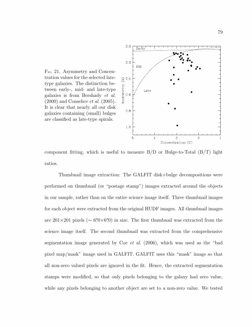
79

FIG. 21. Asymmetry and Concen-tration values for the selected late-type galaxies. The distinction be-tween early-, mid- and late-typegalaxies is from Bershady et al.(2000) and Conselice et al. (2005).It is clear that nearly all our diskgalaxies containing (small) bulgesare classified as late-type spirals.

component fitting, which is useful to measure B/D or Bulge-to-Total (B/T) light

ratios.

Thumbnail image extraction: The GALFIT disk+bulge decompositions were

performed on thumbnail (or “postage stamp”) images extracted around the objects

in our sample, rather than on the entire science image itself. Three thumbnail images

for each object were extracted from the original HUDF images. All thumbnail images

are 201×201 pixels (∼ 6′′.0×6′′.0) in size. The first thumbnail was extracted from the

science image itself. The second thumbnail was extracted from the comprehensive

segmentation image generated by Coe et al. (2006), which was used as the “bad

pixel map/mask” image used in GALFIT. GALFIT uses this “mask” image so that

all non-zero valued pixels are ignored in the fit. Hence, the extracted segmentation

stamps were modified, so that only pixels belonging to the galaxy had zero value,

while any pixels belonging to another object are set to a non-zero value. We tested

80

this GALFIT decomposition with and without bad pixel maps for comparison, and

obtained very similar fitting results. The third thumbnail was extracted from the

drizzle-generated weight image (Koekemoer et al. 2002). These weight images were

modified for GALFIT (C. Peng, private communication) as follows. First, the science

image was smoothed by a few pixels to get rid of some of the random pixel-to-

pixel variations. Second, a variance image S, was calculated using S = (1/wht) +

data/exptime, where, wht is the drizzle-generated weight image, data is the science

image in counts/sec and exptime is the total exposure time of the image. Finally, a

sigma image is generated using σ =√

S. These modified weight images were used as

the input “sigma” image (noise maps) in the GALFIT, which is necessary for proper

error-propagation.

Sky background: The drizzled HUDF images are sky subtracted and therefore,

to understand the effects from the sky-subtraction errors, we used the following pro-

cedure. A careful analysis of the HUDF sky-background and its corresponding uncer-

tainties was performed by Hathi et al. (2008b). We used these sky-background values

from Hathi et al. (2008b), and allowed GALFIT to either vary this sky-level during

the fitting process, or keep it fixed. For comparison, we also used the sky-background

measured from each individual object stamp, and repeated the process. We also

tested our GALFIT decomposition by comparing the results from GALFIT with and

without the addition of the sky-background. We found very consistent and similar

fitting parameters from all these tests. Therefore, we adopted the sky-background

levels measured by Hathi et al. (2008b) in our final GALFIT decomposition.

81

Using GALFIT: GALFIT produces model images of galaxies based on initial

input parameters. These images are convolved with the ACS Point Spread Function

(PSF) image before comparing with the actual galaxy image. Fitting proceeds iter-

atively until convergence is achieved, which normally occurs when the χ2 does not

change by more than 5 parts in 104 for successive five iterations (See Peng et al.

2002). GALFIT requires initial guesses for the fitting parameters. Following Dong &

De Robertis (2006) and Simien & de Vaucouleurs (1986), we used the output param-

eters from the published HUDF SExtractor catalogs (Beckwith et al. 2006) as input

values for the magnitude, the half-light radius, the position angle, and the ellipticity

of each object. The initial value for the Sersic index, n, was taken to be 1.5 (Coe et

al. 2006). Tests based on an adopted initial value of n=4 showed similar results.

All GALFIT measurements were obtained from the V - and z′-band images

(approximately rest-frame U - and B-band, respectively). First, we fitted only an

one-component Sersic profile to our galaxies to improve the initial estimates for the

Sersic index, the axis ratio and the position angle of each galaxy. The distribution

of Sersic indices for our galaxies in the V - and z′-band is shown in Figure 22. Our

measurements of the Sersic index in V - and z′-band are comparable to i′-band values

of the galaxies in Coe et al. (2006). Figure 22 confirms that most of the galaxies in

our sample have a Sersic index n < 2 in both V - and z′-bands, which implies that

our galaxies are disk-dominated, as Figure 18 and Figure 19 clearly suggest.

Next, we simultaneously fitted two components: a Sersic profile plus an expo-

nential disk profile, to get better estimates of the bulge and disk magnitudes, respec-

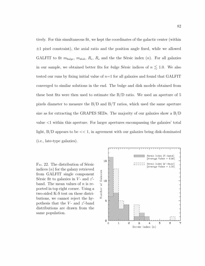
82

tively. For this simultaneous fit, we kept the coordinates of the galactic center (within

±1 pixel constraint), the axial ratio and the position angle fixed, while we allowed

GALFIT to fit mbulge, mdisk, Re, Rs and the the Sersic index (n). For all galaxies

in our sample, we obtained better fits for bulge Sersic indices of n . 1.0. We also

tested our runs by fixing initial value of n=1 for all galaxies and found that GALFIT

converged to similar solutions in the end. The bulge and disk models obtained from

these best fits were then used to estimate the B/D ratio. We used an aperture of 5

pixels diameter to measure the B/D and B/T ratios, which used the same aperture

size as for extracting the GRAPES SEDs. The majority of our galaxies show a B/D

value <1 within this aperture. For larger apertures encompassing the galaxies’ total

light, B/D appears to be << 1, in agreement with our galaxies being disk-dominated

(i.e., late-type galaxies).

FIG. 22. The distribution of Sersicindices (n) for the galaxy retrievedfrom GALFIT single componentSersic fit to galaxies in V - and z′-band. The mean values of n is re-ported in top right corner. Using atwo-sided K-S test on these distri-butions, we cannot reject the hy-pothesis that the V - and z′-banddistributions are drawn from thesame population.

83

4.5. Stellar Population Models

The GRAPES grism spectra were taken at five different position angles (PAs)

to remove any contamination and overlap from nearby objects. We generated one

final spectrum for each galaxy by combining all of the GRAPES spectra obtained at

the 5 different PAs. The combination was performed as a simple averaging operation,

after resampling the spectra onto a common wavelength grid. Portions of spectra

which were contaminated more than 25% (see Pirzkal et al. 2004, for a description)

were not used, unless absolutely necessary. The Poisson errors were propagated, and

the standard deviation of the mean between the 5 individual PAs was computed.

The larger of either the Poisson noise or the standard deviation of the mean was

used in the subsequent analysis. Our goal is to fit stellar population models to the

age-sensitive 4000 A break observed in the GRAPES spectra of these galaxies.

Star formation histories (SFH). — We fit our ACS grism spectra to a grid of

models obtained by combining the simple stellar populations of Bruzual & Charlot

(2003). A standard χ2 method is used. We explore a wide volume of parameter

space in order to infer robust constraints on the possible ages and metallicities of the

stellar populations in the central bulges of these galaxies. This comparison requires a

careful process of degrading the synthetic SED (resolution R ∼ 2000) to the (variable)

resolution of the GRAPES spectra. Special care must be taken with respect to the

change of the Line Spread Function (LSF) with wavelength, which results in both

an effective degradation of the spectral resolution as a function of wavelength, and a

different net spectral resolution with respect to the size of the galaxy. After exploring

84

a range of values R= 30−80, we find that an effective resolution of R = 50 is suitable

for all the spectra in our sample. The ACS grism spectral resolution is not degenerate

with respect to parameters describing the star-formation history, and mostly results

in a global shift of the likelihood.

In order to determine the redshift as accurately as possible, we start with some

guessing values obtained from three sources: a photometric redshift; a VLT spectro-

scopic redshift — where available — and a redshift estimate taken from an automated

method (as discussed in ‘Sample selection’ section) to search for a prominent 4000 A

break in GRAPES data. A small set of templates at the GRAPES resolution were

used to determine the best redshift for each galaxy, using the guessing values de-

scribed above as a starting point, and performing a simple cross-correlation for a

range of redshifts until the best match is found. This method generates the redshifts

used throughout this paper, shown in Table 6 as “SED Fit”.

In order to make a robust assessment of the ages and metallicities of the unre-

solved stellar populations, we use two different sets of models to describe the build up

of the stellar component. The models depend on a reduced set of parameters, which

can characterize a star-formation history in a representative fashion.

Model #1 (EXP): We take a simple exponentially decaying star formation rate,

so that each star-formation history is well parametrized by a formation epoch, which

can be described by a formation epoch (t(zF )); a star-formation timescale (τ⋆ =

0.1 → 4 Gyr); and a metallicity ([m/H ] = −1.5 → +0.3), which is kept fixed at all

times. The numbers in brackets give the range explored in the analysis of the model

85

likelihood. The range in formation epochs is chosen from zF = 10 to t(zF ) = 0.2 Gyr

(this range depends on the observed redshift of the galaxy).

Model #2 (CSP): We follow a consistent chemical enrichment code as described in

Ferreras & Silk (2000). The model allows for gas infall and outflow. The metallicity

evolves according to these parameters, using the stellar yields from Thielemann et

al. (1996) for massive stars (> 10M⊙), and van den Hoek & Groenewegen (1997) for

intermediate mass stars. The free parameters are the formation epoch (same range as

the one chosen for Model #1), the timescale for the infall of gas (τf = 0.1 → 1 Gyr),

and the fraction of gas ejected in outflows (BOUT = 0 → 1). The star-formation

efficiency is kept at a high value CEFF = 20 as expected for early-type populations

(see Ferreras & Silk 2000).

For each of the two sets of models we run a grid of SFHs, convolving simple

stellar populations from the models of Bruzual & Charlot (2003). The grid spans

64 × 64 × 64 SFHs (note that three free parameters are chosen in each set) over a

wide range of values as shown above. Once the best fit is obtained within the grid, we

run a number of models with random values of the parameters with an accept/reject

criterion based on the likelihood – analogous to the Metropolis algorithm, e.g., Saha

(2003). The process ends when 10,000 models are accepted. The total number of

accepted models determine the median and confidence levels of the parameters. The

distribution of reduced χ2 values has an average of χ2=0.74 and RMS σ(χ2) = 0.35.

The χ2 used throughout includes a mild Gaussian prior on the metallicity with average

[m/H]= −0.1 and RMS σ([m/H ]) = 0.5. This prior allows for a relatively wide

86

range of average metallicities, and is compatible with the values commonly found

in these systems (e.g., Carollo et al. 2007). The distribution of bulge metallicities

(log(Z/Z⊙)) estimated from the stellar population models is shown in Figure 23. The

data point shows the average value and rms scatter of the distribution. A mild

Gaussian prior on the metallicity with average [m/H]= −0.1 and RMS σ([m/H ]) =

0.5 is overplotted on the distribution. Figure 23 clearly shows that the metallicity

prior still allows for a wide range of average metallicities. The average metallicities

obtained from our models is comparable with the values obtained at z ≃ 1 from

ground-based spectroscopic observations (e.g., Shapley et al. 2005; Schiavon et al.

2006; Liu et al. 2008), which was our main motivation to include metallicity priors

in first place. Using a flat prior instead yields very similar results.

FIG. 23. The distribution of bulge metal-licities (log(Z/Z⊙)) estimated from thestellar population models. The datapoint shows the average value and rmsscatter of the distribution. We overplot amild Gaussian prior used on the metallic-ity with average [m/H]= −0.1 and RMSσ([m/H ]) = 0.5. It is clearly shownthat this metallicity prior still allows fora wide range of average metallicities, andis compatible with the values obtained atz ≃ 1 from ground-based spectroscopicobservations (e.g., Shapley et al. 2005;Schiavon et al. 2006; Liu et al. 2008).

Figure 24 shows the best fit models and the observed SEDs for 10 galaxies in

our sample. The error bars represent the observations, and the solid line correspond

to the best fits for the CSP model. The wavelength is shown in the observed frame,

87

whereas the wavelength range chosen for all galaxies is 3800–5000 A in the rest-frame.

This choice ensures a consistency in the comparison of the stellar populations in our

sample. The chosen range straddles the age-sensitive 4000 A break.

FIG. 24. Spectral energy distribu-tions of 10 galaxies in our sam-ple (Each one is labeled with theHUDF numbers and model red-shifts). The error bars are the ob-served ACS/G800L data and thelines are the best fits accordingto the CSP models (see text fordetails). The distribution of re-duced χ2 values has an average ofχ2=0.74 and RMS σ(χ2) = 0.35.

Figure 25 shows the 4000 A break amplitude, D4000, as a function of stellar

age. The distribution of bulge ages is overplotted as histogram, which agrees very

well with the range in D4000 (which is 1.2 to 1.5 in general) that we obtain, as shown

in Figure 17. Different curves show three simple stellar population models with three

different metallicities. For metallicity around solar (thick-solid and dashed lines),

which we obtain for our bulges, the variation in D4000 with age is very similar.

For solar metallicity with E(B–V )=0.2 dust reddening (thin-solid line) and for high

metallicity (dotted line), the relation is somewhat steeper. Figure 25 shows that for

the range in D4000 and metallicities of our sample, the effect of metallicity on D4000

small, and D4000 is a good age indicator for this sample.

88

FIG. 25. The D4000 as a function of stellar age. The distribution of bulge ages isoverplotted as histogram, which agrees very well with the range in D4000 (which is1.2 to 1.5) we get as shown in Figure 17. Different curves show three simple stellarpopulation models with three different metallicities. For metallicity around solar(thick-solid and dashed lines), which we are getting for our bulges, the variation inD4000 with age is very similar, and so a slight change in metallicity does not affectD4000. For solar metallicity with 0.2 dust reddening (thin-solid line) and for highmetallicity (dotted line), the relation is little steeper.

Figure 26 shows the ages and metallicities of the best SFHs for each bulge. The

average and RMS scatter for age and metallicity are shown as dots and error bars,

respectively. For the EXP models – which have zero spread in metallicity – the error

bars in metallicity represent the uncertainty estimated from the likelihood. The solid

lines in the lower panels correspond to the age of the Universe as a function of redshift.

89

The dashed lines show the age that a simple stellar population – a population with

a single age – would have if formed at redshifts (from top to bottom) zF = 5, 3, 2.

The median value of the stellar ages of our bulges is 1.3 Gyr. The CSP models

treat chemical enrichment in a more consistent way than the EXP models and should

therefore better reflect the true populations.

FIG. 26. Ages and metallicities corresponding to the best fit according to a simpleexponentially decaying model (EXP; [Left]) or a consistent chemical enrichment code(CSP; [Right]). The filled circles are the average values of age or metallicity andthe error bars represent the RMS of the distribution. The solid lines in the bottompanel track the age of the Universe at a given redshift for a concordance cosmology.The dashed lines – from top to bottom – correspond to formation redshifts of zF =5, 3, 2. The dashed lines correspond to the age of simple stellar populations formedat zF = 5, 3, 2 (i.e., if they had an e-folding timescale τf=0). The triangles are thelower redshift early-type galaxies from Pasquali et al. (2006b), which were analyzedthe same way.

90

We would emphasize here that it is the average stellar age that can be reason-

ably constrained with the data. Therefore, Figure 26 does not imply that all stars in

these bulges are ∼1.3 Gyr but many may be older. To clarify, the formation epoch

(characterized by a formation redshift) is the age when star formation starts in the

model. Figure 27 shows the formation redshift (zF ) and the e-folding timescale (τf )

corresponding to the best fit stellar population models. Here, zF is the epoch at

which the model starts star-formation (as described earlier), and τf is the e-folding

timescale of star-formation, with shorter timescales (.0.5 Gyr) corresponding to a

more elliptical-type old stellar population. We see a large spread in both zF and τf ,

but with a clear indication that most low mass bulges have a more extended star-

formation history (τf & 1 Gyr) and a lower formation redshift (zF . 2.5). Hence,

most of our bulges appear to have an extended SFHs. We also include a characteristic

error bar showing uncertainties in these values.

The best-fit stellar population models show that our bulges have similar ages

independent of redshift. This similarity in ages could be due to two possible reasons.

First, our galaxy sample has a redshift range from z ≃ 0.8 to 1.3, but most of our

galaxies are in much smaller redshift range from z≃0.9 to 1.1. We have applied same

selection criteria to all of our galaxies in a small field so it is possible that we have

selected similar kind of galaxies/bulges with similar bulge ages in this small redshift

range. Secondly, Vanzella et al. (2006) has predicted Large Scale Structure (LSS) in

the CDF-S around z≃1.0 from VLT spectroscopic redshifts. Redshift distribution in

the HUDF (smaller field in the CDF-S) also show a strong peak around z≃ 1.0. So

91

FIG. 27. Formation redshift (zF ) and the e-folding timescale (τf ) corresponding to thebest fit stellar population model. zF is the epoch at which we start star-formation (asdescribed in the text) and τf is the e-folding timescale of star-formation, with shortertimescales corresponding to an elliptical-type old population. There is a large spreadin both zF and τf , but with a clear indication that many low mass bulges may havehad an extended star-formation history (τf & 1 Gyr) and a lower formation redshift(zF . 2.5). We also include a characteristic error bar showing the typical fittinguncertainties in these values.

it is possible that we may be looking at a smaller subset of this LSS at z≃1.0.

Bulge mass estimates. — The photometry from Table 5 can be combined

with the M/L ratios obtained from the best-fit SFH to constrain the stellar mass

(Ms) content of the bulges. This M/L is derived from the composite model obtained

by combining the simple stellar populations from Bruzual & Charlot (2003) using a

Chabrier (2003) Initial Mass Function (IMF). If we change the IMF from Chabrier

(2003) to Salpeter (1955), the stellar mass will increase by ∼0.3 dex in log(Ms), which

within the other errors in data and models, does not change our overall results. The

92

photometry has to be corrected to take into account contamination from the disk.

We use the B/D ratio obtained from the GALFIT to estimate the bulge fraction of

the light in the galaxy. The stellar mass estimates for our bulges are in the range of

6.5≤ log(Ms/M⊙)≤10.0.

Disk contamination. — The best-fit stellar population models to the GRAPES

SEDs suggests that the late-type bulges at z ≃ 1 are young, with an average age of

∼1.3 Gyr. To better understand this result, we first need to quantify the effect of

disk contamination in our measurements. The GRAPES SEDS are extracted from an

aperture of relatively narrow-width aperture (5 pixels in diameter) around the center

of each galaxy. The narrow extraction of the grism spectra is dominated by the bulge

and the inner disk light. The extracted spectra clearly show 4000 A breaks in all

uncontaminated PAs, due to the older stellar population in the central region of the

galaxy. We fit our stellar population models to this break only and hence, we need to

investigate the spectral contamination due to the inner disk in these age estimates.

We perform following photometric tests to understand the effect of the inner disk on

the bulge ages.

(1) We used the disk and bulge light profiles produced by GALFIT and mea-

sured their flux in a strip 5 pixel wide and around their common center, to estimate

the disk and bulge light-fraction within this aperture. We find that the light con-

tributed by the disk to the total flux in this aperture can be as high as 30%. At the

same time, we measured the disk and bulge colors within the same aperture, to find

that the disk and the bulge are similar within the photometric errors, so that the disk

93

contamination in the bulge spectrum is not expected to dominate our estimate of the

bulge age. This can be already be seen in Figure 19, where the bulge is in general

0.3–0.8 mag redder in (V –z′) than the disk.

(2) We compared the bulge age derived from the stellar population models with

the color difference between two apertures. We measure the color difference between

two apertures with 2.5 pixels and 5 pixels radii, equivalent to the narrow and wide

GRAPES spectral extractions, respectively. The top panel of Figure 28 shows the

comparison between the color difference and the bulge age. The points on the plot

are color-coded according to their B/D ratios, measured from GALFIT. Blue color

stands for B/D≤0.5, green means 0.5<B/D≤1 and red represents B/D>1. The top

panel of the Figure 28 does not show any major trends among age, color difference,

and B/D ratio. Secondly, we compared the bulge age to the color difference between

the 2.5 pixels aperture and the annulus defined by the 2.5 and 5 pixels apertures.

The bottom panel of the Figure 28 shows this comparison. The points on the plot are

color-coded according to their B/D ratios, as in the top panel. Like the top panel,

the bottom panel of Figure 28 does not show any major correlation among age, color

difference, and B/D ratio. Finally, we directly compared the B/D ratio with the age

and mass of the bulge. The top panel of Figure 29 shows the comparison between the

B/D ratios obtained from the GALFIT and the bulge age from the stellar population

models for all galaxies in the sample. Figure 29 does not show any correlation between

the age and the B/D ratio. Similarly, the bottom panel of Figure 29 shows at best a

very mild correlation between the bulge stellar mass and the B/D ratio.

94

FIG. 28. Comparison between aperture colors and the best-fit bulge age. [Top] showsthe bulge age as a function of the color difference between the 2.5 pixels apertureand the 5 pixels aperture. [Bottom] shows the bulge age as a function of the colordifference between the 2.5 pixels aperture and the annulus defined by the 2.5 and 5pixels apertures. A blue colored circle stands for B/D≤0.5, green means 0.5<B/D≤1and red represents B/D>1. Here B/D is measured in the i′-band. Both panels doesnot show any correlation among the age, color difference, and B/D ratio.

(3) For a few sample galaxies, we extracted the spectrum of their disk above

and below the bulge aperture used to extract the bulge spectrum, at a distance of

approximately 10 pixels from the galaxy center. Similarly to its bulge, the disk also

exhibits a 4000 A break in the spectrum whose amplitude is only slightly smaller

(within few percents) from that of the bulge. This test shows that both bulges and

inner disks are comparably red/old. We also fitted stellar population models using

both the bulge and disk spectra, and analyzed how the bulge-age and metallicity

95

change as a function of disk contamination, i.e., the fraction of disk light added to

the bulge spectrum. Our simulations show that the determination of the bulge age is

not dominated by disk contamination. Even when disk contamination is completely

ignored – or fully subtracted – the bulge ages do not change much.

FIG. 29. Correlation between measuredB/D ratio from GALFIT and the CSPmodel parameters age and mass. Thetop panel shows that there is no correla-tion between the B/D ratio and the bulgeages for late-type galaxies. The bottompanel shows at best a very mild correla-tion between the B/D ratio and the massof these late-type bulges.

In summary, we do not detect any significant correlation between the bulge

age, B/D ratio and the aperture color difference. We thus conclude that our estimate

of the bulge ages is fairly robust, and that the younger age of the sample bulges is

likely real and not due to disk contamination.

4.6. Discussion

The ages and masses of late-type bulges are estimated by fitting our GRAPES

SEDs with stellar population models. Our analysis shows that bulges in late-type

galaxies at higher redshift (z ≃ 1) appear to be relatively young (average age∼1.3

Gyr) and less massive (6.5 ≤ log(Ms/M⊙) ≤ 10.0) compared to early-type galaxies

at same redshift. This finding appears to be independent of the relative amount of

96

disk-light present, or the color of the underlying disk. Figure 30 shows the stellar

masses of our bulges (filled and open circles) compared with the best-fit ages from

the CSP models. We also include the stellar mass estimates for the elliptical galaxies

from GRAPES/HUDF (grey triangles; Pasquali et al. 2006b), which were analyzed

in a similar way. Their sample of early-type galaxies covers a lower range of redshifts

(0.5 ≤ z ≤ 1.0). Hence, for a proper comparison, we divide our bulges with respect

to redshift: z ≤ 1 (solid circles) and z > 1 (open circles). The bulges in our late-type

spirals span a much lower range of ages, and have lower masses, compared to those

of early-type galaxies.

Elmegreen et al. (2005) have classified ∼900 galaxies (larger than 10 pixels or

0′′.3) in the HUDF according to morphology and their photometric properties. They

find 269 spiral galaxies in the HUDF. Using the Elmegreen et al. (2005) morphological

classifications, and accurate spectro-photometric redshifts from Ryan et al. (2007),

we estimate that the results in this paper represent approximately ∼40–50% of the

total late-type/spirals HUDF galaxy population within the magnitude and redshift

range used in this paper.

Our analysis of the central and the inner disk colors of these galaxies (Figure 19)

and their grism spectra shows that the inner disk and the bulge components have

similar colors, and that the bulge ages are not significantly affected by the light (and

stellar populations) of the underlying disk. This result is consistent with the idea

that the inner disk of galaxies in general has similar colors and age as the bulge (e.g.,

Peletier & Balcells 1996). The effect of dust on these measurements should not be

97

FIG. 30. Comparison between bulges in early-type (grey triangles/dashed lines) andlate-type galaxies (black circles/lines). Measurements for early-type galaxies are dis-cussed in Pasquali et al. (2006b). Inset shows redshift distribution for both thesesamples with ellipticals peaking at z ≃ 0.7. Early-type galaxies are mostly at z < 1,therefore we divide our late-type bulges into z ≤ 1 (filled circles) and z > 1 (opencircles). It is clear that for similar redshifts, bulges in late-type galaxies are youngerand less massive compared to bulges in early-type galaxies.

significant, since our bulge ages are based on the amplitude of the 4000 A observed

in the GRAPES grism spectra, which is sensitive to age rather than to dust. Also,

MacArthur et al. (2004) argue that dust is generally not a significant contributor to

galaxy colors in low-mass/low-luminosity spiral galaxies, but is likely important in

more massive/brighter galaxies. On the other hand, even if dust plays an important

role in this analysis, then inclusion of dust will make our ages still younger, and our

98

result that bulges and inner-disks have similar dominant stellar population with an

average age of ∼1.3 Gyr should then be viewed as an upper limit.

We performed GALFIT decomposition on the sample galaxies by simultane-

ously fitting the bulge to a Sersic profile and the disk to an exponential profile. For all

bulges in our sample, we obtained better fits using Sersic indices of n . 1.0. There-

fore, these bulges are disk-like (Kormendy & Kennicutt 2004; Athanassoula 2005)

and have radial surface brightness profiles similar to disks. Similar analyses for local

spirals by de Jong (1996) and Courteau et al. (1996) have shown that the majority

of bulges in late-type galaxies are better fit by exponential profile. Our results show

that a similar trend also exists at z≃1. The similarities we find in the bulge and the

inner-disk properties (4000 A break, colors and profiles) could imply that these less

massive, younger bulges at z≃1 grow through secular evolution processes (Kormendy

& Kennicutt 2004). At z≃1, it is possible that we are seeing these galaxies still form-

ing, and these “disk-like” bulges might grow from disk material or minor mergers to

become more massive bulges observed at present day. Disk-like pseudo-bulges can

also grow by gas inflow and star-formation. Bars can drive central gas inflows (Sheth

et al. 2005), and therefore, there could be a correlation between these disky bulges

and central bars. Sheth et al. (2008) find that the bar fraction in very massive, lumi-

nous spirals is constant from z ≃ 0 to z ≃ 0.84, whereas for low-mass, blue spirals it

declines significantly with redshift to about ∼20% at z ∼ 0.84, indicating that some

bars do form early enough. Elmegreen et al. (2005) has morphologically classified

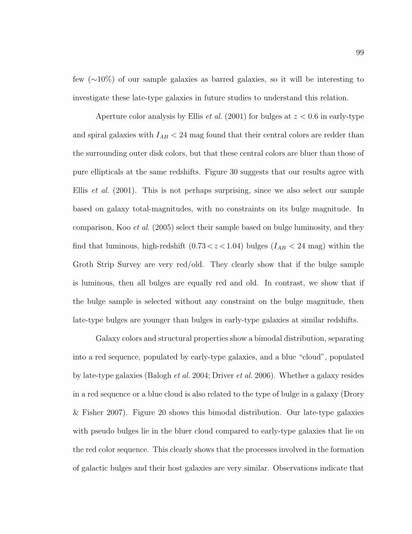
99

few (∼10%) of our sample galaxies as barred galaxies, so it will be interesting to

investigate these late-type galaxies in future studies to understand this relation.

Aperture color analysis by Ellis et al. (2001) for bulges at z < 0.6 in early-type

and spiral galaxies with IAB < 24 mag found that their central colors are redder than

the surrounding outer disk colors, but that these central colors are bluer than those of

pure ellipticals at the same redshifts. Figure 30 suggests that our results agree with

Ellis et al. (2001). This is not perhaps surprising, since we also select our sample

based on galaxy total-magnitudes, with no constraints on its bulge magnitude. In

comparison, Koo et al. (2005) select their sample based on bulge luminosity, and they

find that luminous, high-redshift (0.73<z <1.04) bulges (IAB < 24 mag) within the

Groth Strip Survey are very red/old. They clearly show that if the bulge sample

is luminous, then all bulges are equally red and old. In contrast, we show that if

the bulge sample is selected without any constraint on the bulge magnitude, then

late-type bulges are younger than bulges in early-type galaxies at similar redshifts.

Galaxy colors and structural properties show a bimodal distribution, separating

into a red sequence, populated by early-type galaxies, and a blue “cloud”, populated

by late-type galaxies (Balogh et al. 2004; Driver et al. 2006). Whether a galaxy resides

in a red sequence or a blue cloud is also related to the type of bulge in a galaxy (Drory

& Fisher 2007). Figure 20 shows this bimodal distribution. Our late-type galaxies

with pseudo bulges lie in the bluer cloud compared to early-type galaxies that lie on

the red color sequence. This clearly shows that the processes involved in the formation

of galactic bulges and their host galaxies are very similar. Observations indicate that

100

these formation mechanisms depend strongly on the bulge (as well galaxy) mass, and

that they were active already at z≃1.3. This evidence is strengthened by the results

of Thomas & Davies (2006) and MacArthur et al. (2008), who find that bulges of

similar mass have a similar evolutionary path. Possibly because of cosmic variance,

we do not detect early-type spirals at z≃1 in the HUDF. Comparing our sample of

late-type bulges with the massive early-type galaxies at similar redshifts studied by

Pasquali et al. (2006b), we confirm the existence of different evolutionary tracks for

bulges in early- and late-type galaxies (see Figure 20).

Our analysis of the deepest optical survey, the HUDF, along with the deep

unique ACS grism spectroscopy provides the best spatial resolution at z ≃ 1, and

yields more detailed insight in the process of galaxy formation. Massive and luminous

bulges (e.g., Koo et al. 2005), which mostly reside in early-type galaxies and in earlier-

type spiral galaxies, are old and formed at z&2. The secular evolution suggested by

Kormendy & Kennicutt (2004) does not play any role in their formation. Our ACS

grism study of the HUDF here has shown that lower-mass bulges, which are mostly

associated with later-type galaxies, are younger and form at z.2 possibly via secular

evolution.

5. DISCUSSION & CONCLUSIONS

5.1. Overview

In this final section, a summary of results from three studies investigating

structural and physical properties of high redshift galaxies in the Hubble Ultra Deep

Field (HUDF) is presented. This is followed by a description of the future prospects

for understanding high redshift galaxies using deep ground-based spectroscopy and

new upcoming space-based instruments on the Hubble Space Telescope (HST ) and

the James Webb Space Telescope (JWST ). Deep ground-based spectroscopy from

8m-10m class telescope (e.g., Keck, Very Large Telescope (VLT), Southern African

Large Telescope (SALT), Large Binocular Telescope (LBT)) is necessary to under-

stand physical characteristics of these high redshift galaxies, while upcoming Wide

Field Camera-3 (WFC3) on the HST and Near-Infrared Camera (NIRCam) on the

JWST are necessary to secure multi-wavelength data and morphological information

for many known and yet to be discovered high-redshift galaxies. A preview of what

such observations might show is given by, e.g., Windhorst et al. (2008).

5.2. Summary of Results

Surface brightness profiles at z ≃ 4−6 (chapter 2). — We used the stacked

HUDF images to analyze the average surface brightness profiles of z≃4−6 galaxies

at the HST diffraction limit. Our analysis shows that even the faintest galaxies at

z ≃ 4−6 are resolved. This may have implications for their stellar density and its

relation to the stellar density in present-day galaxies. We also find that the average

surface brightness profiles display “breaks” at a radius that progresses toward lower

redshift from r ≃0′′.27 (1.6 kpc) at z≃6 to r ≃0′′.35 (2.5 kpc) at z≃4.

102

The shape of the radial surface brightness profile that we observe (Figure 10)

could result from a mixture of different morphological types of galaxies, if they existed

at z≃4−6, because we can produce similar breaks in the surface brightness profiles

when we mix different types of nearby galaxies. Alternatively, if these galaxies are

dominated by a central starburst, then they could show such double exponential-

type profiles, as discussed by Hunter & Elmegreen (2006). In a third scenario, if the

galaxies at z≃4 − 6 are truly young and mostly late-type objects, the outer profiles

seen in our mean radial surface-brightness profiles at z ≃ 4 − 6 bear the imprint of

the hierarchical build-up process and are still dominated by in-falling material, which

is not detectable in the individual HUDF images of these faint objects. We have

estimated limits to the dynamical ages from the break radius at z≃4, 5, and 6 very

roughly as ∼0.20, 0.14 and 0.10 Gyr, respectively. These ages are similar to the

Spectral Energy Distribution (SED) ages inferred at z≃4−6 (Yan et al. 2005; Eyles

et al. 2005, 2007), and they are consistent with SED ages suggested for z≃7 (Labbe

et al. 2006). Hence, at z ≃ 4, 5, 6, the last major merger that affected the surface

brightness profiles that we observe, and that triggered the observed star-burst, may

have occurred respectively ∼0.20, 0.14 and 0.10 Gyr earlier, or very approximately at

z ≃ 4.5, 5.5, 6.5. This would be consistent with the hierarchical assembly of galaxies

and with the end of the epoch of reionization, since it would imply that going from

z≃4 to z≃6, the SEDs become progressively more dominated by late-B–late-O stars.

This, in turn, implies that sub-L∗ (i.e., dwarf) galaxies may have produced sufficient

numbers of energetic UV photons to complete the reionization process by z ≃ 6, as

103

Yan & Windhorst (2004a,b) suggested. It will be imperative to study with future

instruments like HST/WFC3 and JWST (Windhorst et al. 2006, 2008) whether the

dominant stellar population indeed changes from late-O–early-B at z≃6 (i.e., capable

of reionizing) to mid- to late-B at z≃4−5 (i.e., capable of maintaining reionization),

and to what extent the intrinsic sizes of these faint objects will ultimately limit deep

JWST surveys.

Starburst intensity limit at z≃5−6 (chapter 3). — We have measured the star-

burst intensity limit for spectroscopically confirmed galaxies at z≃5−6 from Advanced

Camera for Surveys (ACS) grism survey GRism ACS Program for Extragalactic Sci-

ence (GRAPES) in the HUDF. We find that there is little variation in the upper limit

of the surface brightness from z≃3 to z≃6, and that the starburst intensity limit is

within a factor of 3 when compared with the sample of z≃3−4 galaxies (Figure 15).

The constancy of the starburst intensity limit for starburst galaxies at z ≃ 5−6 —

combined with the results obtained by Meurer et al. (1997) for starbursts at z.3 —

implies that the physical processes limiting the starburst intensity at lower redshifts

also apply to these high redshift galaxies. We find that the high redshift starbursts

have a smaller characteristic linear size than their local counterparts, and a corre-

spondingly lower luminosity (since their maximum surface brightnesses are similar

and their sizes smaller). We observe the apparent galaxy size evolution from z≃3 to

z ≃ 6 and find that the sizes scale approximately as the Hubble parameter H−1(z).

Finally, using rest-frame UV colors, we conclude that the evolution in the UV spectral

slope from z≃3 to z≃6 reinforces the evolution of dust, which leads to bluer galaxies

104

at z ≃ 5−6 compared to galaxies at z ≃ 3. This implies that starbursts were less

obscured, when the universe was younger and had lower heavy element abundances.

Any future search for galaxies at higher redshifts (e.g., JWST ; Windhorst et al. 2008)

needs to take into account the size evolution and constancy of the maximum surface

brightness, and therefore the decrease in characteristic luminosity with redshift.

Late-type galaxies at z ≃ 1 (chapter 4). — We have estimated the stellar

ages and masses of 34 bulges of late-type galaxies observed in the HUDF by fitting

stellar population models to the 4000 A break observed in the GRAPES grism spectra

(Figure 26). This study takes advantage of the exceptional angular resolution and

depth of the GRAPES/HUDF data which allow us to identify the bulge component

of the sample galaxies at z ≃ 1 both on the direct HST and on the ACS grism

images, and to extract its corresponding spectrum. We find that bulges in late-type

galaxies at high redshift (z≃1) appear to be predominantly young (with an average

age∼1.3 Gyr) and less massive (6.5≤ log(Ms/M⊙)≤ 10.0) than bulges in early-type

galaxies at the same redshift. This finding is robust against the amount of disk-light

underneath the bulge light. Our results support the scenario where low-mass late-type

bulges formed through secular evolution processes, perhaps driven by minor mergers

or infall.

5.3. Future Work

In the past decade, ground and space-based observations of high redshift galax-

ies have begun to disentangle the process of galaxy assembly. The details of that pro-

cess at high redshifts, however, remain poorly constrained. There is presently little

105

information on the dynamical structure of these or other galaxies at z≃6. It is not

clear whether these objects represent isolated disk systems, or collapsing spheroids,

mergers, and/or other dynamically young objects. Distinction between these possible

morphologies and, therefore, a better estimate of the formation redshifts of the sys-

tems observed at z≃4−6 in particular, is important for testing the galaxy assembly

picture, and for the refinement of galaxy formation models.

We cannot compare structure formation calculations to the observed galaxy

populations without knowledge of their star formation processes. It is therefore

essential to directly measure the properties of star-formation events in the distant

universe, and see how they compare with their nearby counterparts. Projects like

the GRAPES in the HUDF and the Probing Evolution And Reionization Spectro-

scopically (PEARS) in the Great Observatories Origins Deep Survey (GOODS) fields

provide excellent samples of faint spectroscopically confirmed high redshift galaxies

(Malhotra et al. 2005; Hathi et al. 2008a; Malhotra et al. 2008), along with the brighter

Lyman-break galaxies (LBGs)/Lyman-α Emitters (LAEs) confirmed by ground-based

telescopes at z≥4.5.

Future science goals are to characterize the star-formation properties, dust con-

tent, the stellar populations and the rest-frame ultraviolet (UV)/optical morphologies

for large numbers of spectroscopically confirmed LBGs at z ≥ 4.5. To accomplish

these goals, we will use deep WFC3 Near-Infrared (NIR) images from the HST, deep

NIR ground-based spectroscopy (using 8m-10m class telescopes) and mid Infrared

(IR) data from the Spitzer Space Telescope (Spitzer). Future NIR imaging and spec-

106

troscopic instruments such as LBC and/or LUCIFER on 2×8.4m Large Binocular

Telescopes (LBT) will be an additional asset to this proposed research. These goals

are inter-related research areas in which, existing and upcoming instruments will play

major role addressing the issues of star-formation process and structural evolution in

high redshift galaxies.

Starburst activity and stellar population at z≃5−6. — Studies of low redshift

starbursts have established that the UV spectral slope (β) is a good indicator of dust

reddening, and correlates with the far-IR emission from dust (Meurer et al. 1997).

There are many indications that galaxies at z≃5−6 are bluer in the UV than z≃3−4

galaxies (e.g., Stanway et al. 2005; Bouwens et al. 2006). We (Hathi et al. 2008a,

Chapter 3) find that the UV slope of z≃5−6 galaxies (β ≃ −1.70) is bluer than that

of z≃3 galaxies (β ≃ −1.10), although the current sample size remains too small for

definite conclusions. This we intend to improve upon drastically in next few years

with the HST/WFC3.

Estimation of dust extinction is important for measuring the star-formation

rate (SFR) from the UV continuum. Heckman (2005) has proposed that the most

useful parameter to compare local starbursts with physically similar galaxies at high-

z is its ‘intensity’ (i.e., SFR/area). We (Hathi et al. 2008a, Chapter 3) measured an

upper limit to the starburst intensity for LBGs at z≃4−6, and when we combine our

results with those of Meurer et al. (1997) at z≃0−3, we find that this starburst inten-

sity limit does not change much between z≃0 and 6. Does this mean that physical

mechanisms (e.g., galactic winds) limiting this starburst intensity occur similarly for

107

local and high-z starbursts? At the moment, we don’t know. Proposed observations

of high-z galaxies with the HST/WFC3 will help to understand these details.

To identify “old” stellar populations (i.e., stars older than 108 years) or dusty

star formation regions, we need to observe high redshift (z≃5−6) galaxies at their rest-

frame optical wavelengths. NIR and mid IR observations are essential to accurately

determine their SEDs and rest-frame optical properties. At the redshift of these

galaxies, the (H–3.6µm) color constrains the 4000 A break, and thus can accurately

constrain the population of old stars (e.g., Yan et al. 2005). At these redshifts and flux

levels, there is no better way to constrain the presence of old stars than to combine

NIR and mid IR fluxes to measure the 4000 A break before the launch of JWST.

We are presently involved in the HST/ACS PEARS project, which through

low-resolution HST grism spectroscopy in GOODS-S and GOODS-N has identified

and confirmed &100 galaxies at z ≥ 4.5. The rest-frame UV continuum of these

galaxies correspond to the NIR observed-frame. Using deep, high resolution HST J ,

H images, we will obtain very accurate NIR fluxes to measure the UV spectral slope β

(which measures dust) and the corresponding starburst intensity limit for these high-

z galaxies. Low-resolution grism spectra will also be used to confirm the measured

UV slope. We will use deep ground-based spectroscopy to measure a wide variety

of physical parameters for these galaxies: confirm their redshifts, make independent

estimate of β, measure linewidths and/or rotation velocities in many cases, dynamical

masses, equivalent widths of their emission lines, their metallicities and SFRs for

these galaxies. Spitzer/IRAC fluxes will be obtained from the deep archival data

108

in the GOODS (PI: M. Dickinson). Combining HST, Spitzer and grism data, we

can estimate ages and masses of their dominant stellar populations in these galaxies.

If we identify old stellar populations (i.e., age > 3×108 years) in spectroscopically

confirmed L∗ galaxies at z≃5−6, we immediately know that they formed at redshifts

zform & 7−8, and so we can estimate their contribution to the reionizing photon

budget at z > 7 (e.g., Yan & Windhorst 2004a).

Surface brightness (SB) profiles of galaxies at z≃4–6. — The HUDF, GOODS

and deep ACS/WFC parallel fields contain &500 objects (Beckwith et al. 2006;

Bouwens et al. 2006, 2007; Yan & Windhorst 2004a,b) which are B, V , i′-band

dropouts, making them candidates for galaxies at z ≃ 4,5,6, respectively. Despite

the depth (to AB.27–29.5 mag) of these HST fields, however, these objects appear

very faint, with little discernable structural detail.

The similarity in flux and appearance of many of the z≃ 6 candidates in the

HUDF identified by Yan & Windhorst (2004b) suggested that it may be possible to

gain information about their dynamical structure, by creating composite images from

objects that are matched in flux, shape and size. Such a composite would effectively

correspond to a single galaxy detectable at a much higher signal-to-noise (S/N) ratio,

equivalent to ∼4500 HST orbits (∼3000 hrs) on a single such object. At AB≃27–29.5

mag, measuring reliable radial SB profiles is not possible for most individual objects,

but a composite radial profile has much higher S/N and could be meaningful, as long

as the objects are intrinsically similar and at the same redshift.

109

We (Hathi et al. 2008b, Chapter 2) conducted a preliminary study by stacking

a small numbers (30 objects at each redshift bin at z≃4, 5, 6) of compact and isolated

z≃4–6 galaxy candidates in the HUDF to study their average radial SB profiles. Our

results show that image stacking provides reliable, reproducible average SB-profiles.

The shape of the average SB profiles shows that even the faintest z≃4−6 objects are

resolved at the HST diffraction limit. The mean SB profiles shows that the average

compact galaxy at z≃4−6 is clearly extended with respect to the ACS Point Spread

Function (PSF), and can be fitted to a r1/n profile to a radius of r ≃0′′.35–0′′.27.

The radius at which the profile starts to deviate from r1/n (e.g., r ≃0′′.31 for z ≃ 5)

may put an important constraint to the dynamical time scale of the system. The

average profiles and the observed deviations could help us to gain insight into the

stellar population that dominate the inner profiles. This method could provide an

independent way of estimating ages of these stellar populations, and thus far seems

to suggest dynamical ages of 0.2-0.1 Gyr, i.e., similar to their SED ages at these

redshifts.

We can apply this approach on large number of ‘dropouts’ from the HUDF,

GOODS and deep ACS/WFC parallel fields to undertake a much more detailed and

comprehensive analysis, to conclusively establish what is the physical significance

of these composite radial light-profiles of z ≃ 4–6 objects. We can use previously

discussed PEARS/GRAPES projects and deep NIR spectroscopy to confirm many

of these faint ‘dropouts’, and understand any evolution in their rest-frame average

UV SB profiles from z≃6 to z≃4. In future, the 6.5 meter JWST can confirm our

110

results at 1µ in ∼250 hrs. Therefore, we will use this large high-resolution space-

based IR telescope to investigate the morphological structure of individual galaxies

at z≃6. The JWST, to be launched in 2013, will accomplish that in (1/12)th of the

time compared to present capabilities. It is therefore critical that JWST be designed

and built to allow to do ultra-deep near-mid IR surveys, and subtract the sky to a

precision better than 10−3 of the zodiacal foreground.

REFERENCES

Abraham, R. G., Ellis, R. S., Fabian, A. C., et al. 1999, MNRAS, 303, 641

Adelberger, K. L., & Steidel, C. C. 2000, ApJ, 544, 218

Athanassoula, E. 2005, MNRAS, 358, 1477

Athanassoula, E. 2008, IAU Symposium 245 “Galactic bulges”, M. Bureau et al. eds(arXiv:0802.0151)

Balogh, M.L., Morris, S. L., Yee, H. K. C., et al. 1999, ApJ, 527, 54

Balogh, M.L., Baldry, I. K., Nichol, R., et al. 2004, ApJ, 615, L101

Baugh, C. M., Cole, S., & Frenk, C. S. 1996, MNRAS, 283, 1361

Beckwith, S., Stiavelli, M., Koekemoer, A. M., et al. 2006, AJ, 132, 1729

Benitez, N. 2000, ApJ, 536, 571

Bershady, M. A., Jangren, A., & Conselice, C. J. 2000, AJ, 119, 2645

Bertin, E., & Arnouts, S. 1996, A&AS, 117, 393

Binney, J. J., & Tremaine, S. 1987, Galactic Dynamics (Princeton: Princeton Univ.Press)

Bolzonella, M., Miralles, J. M., & Pello, R. 2000, A&A, 363, 476

Bouwens, R., Cayon, L., & Silk, J. 1999, ApJ, 516, 77

Bouwens, R., Illingworth, G. D., Thompson, R. I., et al. 2004a, ApJ, 606, L25

Bouwens, R. J., Illingworth, G. D., Blakeslee, J. P., et al. 2004b, ApJ, 611, 1

Bouwens, R. J., Illingworth, G. D., Blakeslee, J. P., et al. 2006, ApJ, 653, 53

Bouwens, R. J., Illingworth, G. D., Franx, M., et al. 2007, ApJ, 670, 928

Brandt, W. N., Hornschemeier, A. E., Schneider, D. P., et al. 2001, ApJ, 558, L5

Bruzual, G., & Charlot, S. 2003, MNRAS, 344, 1000

Bunker, A. J., Stanway, E. R., Ellis, R. S., et al. 2004, MNRAS, 355, 374

Calzetti, D., Kinney, A. L., & Storchi-Bergmann, T. 1994, ApJ, 429, 582

Carollo, C. M., Scarlata, C., Stiavelli, M., et al. 2007, ApJ, 658, 960

Chabrier, G. 2003, PASP, 115, 763

112

Coe, D., Benitez, N., Sanchez, S. F., et al. 2006, AJ, 132, 926

Conselice, C. J., Bershady, M. A., & Jangren, A. 2000, ApJ, 529, 886

Conselice, C. J. 2003, ApJS, 147, 1

Conselice, C. J., Blackburne, J. A., & Papovich, C. 2005, ApJ, 620, 564

Courteau, S., de Jong, R. S., & Broeils, A. H. 1996, ApJ, 457, L73

Cowie, L. L., Songaila, A., Hu, E. M., et al. 1996, AJ, 112, 839

Davis, M., & Peebles, P. J. M. 1983, ApJ, 267, 465

Davis, M., Guhathakurta, P., Konidaris, N. P., et al. 2007, ApJ, 660, L1

de Jong, R. S. 1996, A&AS, 118, 557

Dong, X. Y. & De Robertis, M. M. 2006, AJ, 131, 1236

Dow-Hygelund, C., Holden, B., Bouwens, R., et al. 2007, ApJ, 660, 47

Driver, S. P., Windhorst, R. A., & Griffiths, R. E. 1995, ApJ, 453, 48

Driver, S. P., Fernandez-Soto, A., Couch, W. J., et al. 1998, ApJ, 496, L93

Driver, S. P., Allen, P. D., Graham, A. W., et al. 2006, MNRAS, 368, 414

Drory, N. & Fisher, D. B. 2007, ApJ, 664, 640

Ellis, R. S., Abraham, R. G., & Dickinson, M. 2001, ApJ, 551, 111

Elmegreen, D. M., Elmegreen, B. G., Rubin, D. S., et al. 2005, ApJ, 631, 85

Eyles, L. P., Bunker, A. J., Stanway, E. R., et al. 2005, MNRAS, 364, 443

Eyles, L. P., Bunker, A. J., Ellis, R. S., et al. 2007, MNRAS, 374, 910

Fan, X., Strauss, M. A., Becker, R. H., et al. 2006, AJ, 132, 117

Ferguson, H. C., Dickinson, M., Giavalisco, M., et al. 2004, ApJ, 600, L107

Fernandez-Soto, A., Lanzetta, K. M., & Yahil, A. 1999, ApJ, 513, 34

Ferreras, I., & Silk, J. 2000, MNRAS, 316, 786

Ferreras, I., Lisker, T., Carollo, C. M., et al. 2005, ApJ, 635, 243

Georgakakis, A., Hopkins, A. M., Sullivan, M., et al. 2003, MNRAS, 345, 939

113

Giavalisco, M., Steidel, C. C., & Macchetto, F. D. 1996, ApJ, 470, 189

Giavalisco, M., Ferguson, H. C., Koekemoer, A. M., et al. 2004a, ApJ, 600, L93

Giavalisco, M., Dickinson, M., Ferguson, H. C., et al. 2004b, ApJ, 600, L103

Gonzaga, S., et al. 2005, “ACS Instrument Handbook”, Version 6.0, (Balti-more:STScI)

Grazian, A., Fontana, A., de Santis, C., et al. 2006, A&A, 449, 951

Guzman, R., Gallego, J., Koo, D. C., et al. 1997 ApJ, 489, 559

Hathi, N. P., Malhotra, S., & Rhoads, J. 2008a, ApJ, 673, 686

Hathi, N. P., Jansen, R. A., Windhorst, R. A., et al. 2008b, AJ, 135, 156

Hathi, N. P., Ferreras, I., Pasquali, A., et al. 2008c, ApJ, accepted (arXiv:0805.0791)

Heavens, A., Panter, B., Jimenez, R., et al. 2004, Nature, 428, 625

Heckman, T. M., Armus, L., & Miley, G. K. 1990, ApJS, 74, 833

Heckman, T. M., Lehnert, M. D., Strickland, D. K., et al. 2000, ApJS, 129, 493

Heckman, T. M. 2001, in ASP Conf. Ser. 240, Gas and Galaxy Evolution, ed. J. E.Hibbard, M. Rupen, & J. H. van Gorkom (San Francisco: ASP), 345

Heckman, T. M. 2005, ASSL, 329, 3

Hernquist, L. & Mihos, J. C. 1995, ApJ, 448, 41

Holwerda, B. W. 2005, (arXiv:0512139)

Hu, E. M., Cowie, L. L., McMahon, R. G., et al. 2002, ApJ, 568, L75

Huchra, J. P., Davis, M., Latham, D., et al. 1983, ApJS, 52, 89

Hunter, D. A., & Elmegreen, B. G. 2006, ApJS, 162, 49

Jansen, R. A. & Kannappan, S. J. 2001, Ap&SS, 276, 1151

Jansen, R. A., Franx, M., Fabricant, D., et al. 2000a, ApJS, 126, 271

Jansen, R. A., Fabricant, D., Franx, M., et al. 2000b, ApJS, 126, 331

Kannappan, S. J., Jansen, R. A., & Barton, E. J. 2004, AJ, 127, 1371

Kauffmann, G., White, S. D. M., & Guiderdoni, B. 1993, MNRAS, 264, 201

114

Kauffmann, G., Heckman, T. M., White, S. D. M., et al. 2003, MNRAS, 341, 33

Kennicutt, R. C., Jr. 1998, ARA&A, 36, 189

Kinney A. L., Calzetti D., Bohlin R. C., et al. 1996, ApJ, 467, 38

Kodaira, K., Taniguchi, Y., Kashikawa, N., et al. 2003, PASJ, 55, L17

Kodama, T., Yamada, T., Akiyama, M., et al. 2004, MNRAS, 350, 1005

Koekemoer, A. M., Fruchter, A. S., Hook, R. N., et al. 2002, The 2002 HST Calibra-tion Workshop, ed. S. Arribas, A. Koekemoer, and B. Whitmore (Baltimore:STScI),337

Koo, D. C., Simard, L., Willmer, C. N. A., et al. 2005, ApJS, 157, 175

Kormendy, J. 1977, ApJ, 218, 333

Kormendy, J. & Kennicutt, R. C. 2004, ARA&A, 42, 603

Kron, R. G. 1980, ApJS, 43, 305

Kurk, J. D., Cimatti, A., di Serego A, S., et al. 2004, A&A, 422, L13

Labbe, I., Bouwens, R., Illingworth, G. D., et al. 2006, ApJ, 649, L67

Lehnert, M. D., & Heckman, T. 1996, ApJ, 472, 546

Lehnert, M. D., Bremer, M., Verma, A., et al. 2007, in ASP Conf. Ser., PathwaysThrough an Eclectic Universe, ed. J. H. Knappen, T. J. Mahoney, & A. Vazedekis(arXiv:0708.3000)

Leitherer, C., Schaerer, D., Goldader, J. D., et al. 1999, ApJS, 123, 3

Liu, X., Shapley, A., Coil, A., et al. 2008, ApJ, 678, 758

Lynden-Bell, D. 1967, MNRAS, 136, 101

MacArthur, L. A., Courteau, S., Bell, E., et al. 2004, ApJS, 152, 175

MacArthur, L. A., Ellis, R. S., Treu, T., et al. 2008, ApJ, 680, 70

Madau, P. 1995, ApJ, 441, 18

Malhotra, S., Rhoads, J. E., Pirzkal, N., et al. 2005, ApJ, 626, 666

Malhotra, S., Pirzkal, N., Rhoads, J., et al. 2008, ApJ, in preparation

Maraston, C. 2005, MNRAS, 362, 799

115

Marzke, R. O., Huchra, J. P. & Geller, M. J. 1994, ApJ, 428, 43

McCarthy, P. J. 2004, BAAS, 36, 1555

Menanteau, F., Abraham, R. G., & Ellis, R. S. 2001, MNRAS, 322, 1

Meurer, G. R., Heckman, T. M., Leitherer, C., et al. 1995, AJ, 110, 2665

Meurer, G. R., Heckman, T. M., Lehnert, M. D., et al. 1997, AJ, 114, 54 (M97)

Meurer, G. R., Heckman, T. M., & Calzetti, D. 1999, ApJ, 521, 64

Mobasher, B., Idzi, R., Benitez, N., et al. 2004, ApJ, 600, L167

Mobasher, B., Capak, P., Scoville, N., et al. 2007, ApJS, 172, 117

Nandra, K., Mushotzky, R. F., Arnaud, K., 2002, ApJ, 576, 625

Oke, J. B., & Gunn, J. E. 1983, ApJ, 266, 713

Padmanabhan, N., Seljak, U., Strauss, M. A., et al. 2004, New Astronomy, 9, 329

Panter, B., Jimenez, R., Heavens, A. F., et al. 2007, MNRAS, 378, 1550

Pascarelle, S. M., Windhorst, R. A., Keel, W. C., et al. 1996, Nature, 383, 45

Pasquali, A., Pirzkal, N., Larsen, S., et al. 2006a, PASP, 118, 270

Pasquali, A., Ferreras, I., Panagia, N., et al. 2006b, ApJ, 636, 115

Peletier, R. F. & Balcells, M. 1996, AJ, 111, 2238

Peng, C. Y., Ho, L. C., Impey, C. D., et al. 2002, AJ, 124, 266

Petrosian, V. 1976, ApJ, 209, L1

Pirzkal, N., Xu, C., Malhotra, S., et al. 2004, ApJS, 154, 501

Pirzkal, N., Sahu, K. C., Burgasser, A., et al. 2005, ApJ, 622, 319

Pirzkal, N., Malhotra, S., Rhoads, J., et al. 2007, ApJ, 667, 49

Ravindranath, S., Giavalisco, M., Ferguson, H. C., et al. 2006, ApJ, 652, 963

Rhoads, J. E., Xu, C., Dawson, S., et al. 2004, ApJ, 611, 59

Rhoads, J. E., Malhotra, S., Pirzkal, N., et al. 2008, ApJ, submitted (arXiv:0805.1056)

Rix, H-W., Barden, M., Beckwith, S., et al. 2004, ApJS, 152, 163

116

Ryan, R. E., Jr., Hathi, N. P., Cohen, S. H., et al. 2005, ApJ, 631, L159

Ryan, R. E., Jr., Hathi, N. P.; Cohen, S. H., et al. 2007, ApJ, 668, 839

Sersic, J. L. 1968, Atlas de galaxias australes

Saha, P. 2003, Principles of Data Analysis, Cappella Archive.

Salpeter, E. E. 1955, ApJ, 121, 161

Schiavon, R., Faber, S. M., Konidaris, N., et al. 2006, ApJ, 651, L93

Scoville, N., Abraham, R. G., Aussel, H., et al. 2007, ApJS, 172, 150

Shapley, A. E., Coil, A., Ma, C-P., et al. 2005, ApJ, 635, 1006

Sheth, K., Vogel, S. N., Regan, M. W., et al. 2005, ApJ, 632, 217

Sheth, K., Elmegreen, D. M., Elmegreen, B. G., et al. 2008, ApJ, 675, 1141

Simien, F., & de Vaucouleurs, G. 1986, ApJ, 302, 564

Sparks, W. B., et al. 2001, ACS Default (Archival) Pure Parallel Program (ISR01-06)

Spergel, D. N., Bean, R., Dore, O., et al. 2007, ApJS, 170, 377

Stanway, E. R., McMahon, R. G., & Bunker, A. J. 2005, MNRAS, 359, 1184

Steidel, C. C. & Hamilton, D. 1992, AJ, 104, 941

Steidel, C. C., & Hamilton, D. 1993, AJ, 105, 2017

Steidel, C. C., Giavalisco, M., Pettini, M., et al. 1996a, ApJ, 462, L17

Steidel, C. C., Giavalisco, M., Dickinson, M., et al. 1996b, AJ, 112, 352

Steidel, C. C., Adelberger, K. L., Giavalisco, M., et al. 1999, ApJ, 519, 1

Stern, D., Yost, S. A., Eckart, M. E., et al. 2005, ApJ, 619, 12

Stetson, P. B. 1987, PASP, 99, 191

Taniguchi, Y., Ajiki, M., Nagao, T., et al. 2005, PASJ, 57, 165

Taylor-Mager, V. A., Conselice, C. J., Windhorst, R. A., et al. 2007, ApJ, 659, 162

Thielemann, F-K., Nomoto, K., & Hashimoto, M. 1996, ApJ, 460, 408

Thomas, D., & Davies, R. L. 2006, MNRAS, 366, 510

117

Thompson, R. I., Illingworth, G., Bouwens, R., et al. 2005, AJ, 130, 1

Tolman, R. C. 1930, PNAS, 16, 511

Tolman, R. C. 1934, Relativity, Thermodynamics, & Cosmology, (Oxford: OxfordUniv. Press), 467

van Albada, T. S. 1982, MNRAS, 201, 939

van den Bosch, F. C. 1998, ApJ, 507, 601

van den Hoek, L. B., & Groenewegen, M. A. T. 1997, A&AS, 123, 305

van Dokkum, P. G., Forster, S., Natascha, M., et al. 2003, ApJ, 587, L83

van Dokkum, P. G., Franx, M., Forster, S., et al. 2004, ApJ, 611, 703

Vanzella, E., Cristiani, S., Dickinson, M., et al. 2006, A&A, 454, 423

Vanzella, E., Cristiani, S., Dickinson, M., et al. 2008, A&A, 478, 83

Vazquez, G. A., & Leitherer, C. 2005, ApJ, 621, 695

Weedman, D. W., Wolovitz, J. B., Bershady, M. A., et al. 1998, AJ, 116, 1643 (W98)

White, R. L., Helfand, D. J., Becker, R. H., et al. 2007, ApJ, 654, 99

Williams, R. E., Blacker, B., Dickinson, M., et al. 1996, AJ, 112, 1335

Windhorst, R. A., Gordon, J. M., Pascarelle, S. M., et al. 1994, ApJ, 435, 577

Windhorst, R. A., Keel, W. C., & Pascarelle, S. M. 1998, ApJ, 494, 27

Windhorst, R. A., Taylor, V. A., Jansen, R. A., et al. 2002, ApJS, 143, 113

Windhorst, R. A., Cohen, S. H., Jansen, R. A., et al. 2006, NewAR, 50, 113

Windhorst, R. A., Hathi, N. P., Cohen, S. H., et al. 2008, Advances in Space Research,41, 1965

Wright, E. L. 2006, PASP, 118, 1711

Yan, H., Windhorst, R. & Cohen, S. 2003, ApJ, 585, L93

Yan, H. & Windhorst, R. 2004a, ApJ, 600, L1

Yan, H. & Windhorst, R. 2004b, ApJ, 612, L93

Yan, H., Dickinson, M., Stern, D., et al. 2005, ApJ, 634, 109

118

Yan, H., Hathi, N. P., & Windhorst, R. A. 2008, ApJ, 675, 136

York, D. G., Adelman, J., Anderson, J. E., Jr., et al. 2000, AJ, 120, 1579

Zibetti, S., White, S. D. M., & Brinkmann, J. 2004, MNRAS, 347, 556