STRATEGY - Miami

STRATEGY

Strategy deals with managerial decisions when other firms (or persons) change their

behavior in response to your behavior. The key question is: how will other firms

react to my decisions?” We would like to:

• Predict how other firms react to our decisions.

• Make decisions accounting for the reaction of others.

For example, in the last section we learned that demand for a firm’s product depends on

what competitors charge. But the competitor’s price was held fixed. We did not consider

that, if we change our price, competitors may match our price change. In order to really

assess the value of, say, cutting prices, we need to consider what others will do in response

to our actions.

You must always ask yourself: “suppose I do x, how will my competitors react?” To

answer this question we will use game theory.

I Framework: Two Player Games, Simultaneous Move

We start with a game with one other player. The other player could be another firm or

another person.

A Payoff matrix

Definition 31 The payoff matrix lists all rewards that each player gets as a function of

decisions made by all players.

For example, consider a price war game. Apple and Samsung are the dominant firms in

the cell phone industry. Because of antitrust laws, Apple and Samsung are forbidden from

colluding to raise prices or even from discussing prices.

• If Apple cuts prices and Samsung does not, Apple can take the majority of the market

share and make a large profit, say $6 million, while Samsung loses $1 million.

• If Samsung cuts prices and Apple do not, then Samsung gains market share and makes

$4 million. However, Apple still makes $1 million, as it has some loyal customers that

will not be attracted to Samsung’s low price.

67

• If both firms cut prices, profits are zero for both firms.

• If both firms do not cut prices, the market is split between the two firms, but the

relatively high prices allows each firm to make a profit of $3 million.

Samsung

Hold prices Cut prices

Apple Hold prices 3,3 1,4

Cut prices 6,-1 0,0

Table 16: Payoff matrix for the price war game.

• Notice that the first number is always the payoff of the firm listed on the left (rows),

• the second number is the payoff of the firm listed on top (columns).

The payoffs depend on the other players actions. If Apple holds prices, the payoff to Apple

depends on what Samsung does.

B Dominant Strategy

If your best action is independent of what the other player does, then the decision is easy.

Definition 32 A Dominant Strategy is an action that is at least as good as all other

actions regardless what the opposing player chooses.

For example in the price war game (table 16),

• Suppose Samsung elects to hold prices. Apple should cut prices and steal Samsung’s

customers, since $6 million is greater than $3 million in the payoff matrix (first column

of table 16).

• Suppose Samsung cuts prices. Then Apple should hold prices, since $1 million is

greater than $0 (second column of table 16).

Thus Apple does not have a dominant strategy: the optimal decision depends on what

Samsung does. Samsung does have a dominant strategy, however:

• If Apple holds prices, Samsung should cut prices and steal business away from Apple

($4 million is greater than $3 million, first row of table 16).

68

• If Apple cuts prices, then Samsung does better by cutting prices (second row, $0>$-1),

splitting the market and making no profit is better than losing $1 million.

So the dominant strategy of cutting prices generates the highest possible profits for Samsung

regardless of the actions of Apple. Apple should then predict Samsung will cut prices.

However, we still do not have a prediction for what Apple will do.

C Nash Equilibrium

We would like to compute the optimal strategy when no dominant strategy exists for at least

one of the players. The trick is to predict the behavior of the other firm. In the the price

war game with payoff matrix given in table 16:

• Apple should predict that Samsung will cut prices. After all, cutting prices is the

dominant strategy for Samsung, regardless of what Apple does.

• Given that Samsung will cut prices, Apple should hold prices.

• The last step is to check if the prediction is accurate: if Apple holds prices then

Samsung will certainly do better by cutting prices, so our prediction that Samsung

will cut prices is correct.

Therefore the optimal strategy for Apple is to hold prices and the optimal strategy for

Samsung is to cut prices. Together, these strategies are a Nash equilibrium and what we

expect to see.

Now let us show that in equilibrium Apple does not cut prices.

• Apple predicts Samsung will hold prices (this is the only prediction that induces Apple

to cut prices).

• Therefore, Apple cuts prices.

• Then Samsung responds by cutting prices.

• But then Apple’s prediction is not correct. Apple in fact prefers to hold prices here.

Apple made the wrong decision because their prediction was not accurate.

So cutting prices is not a Nash equilibrium strategy for Apple, since the prediction is incor-

rect. The incorrect prediction leads Apple to make the wrong decision.

69

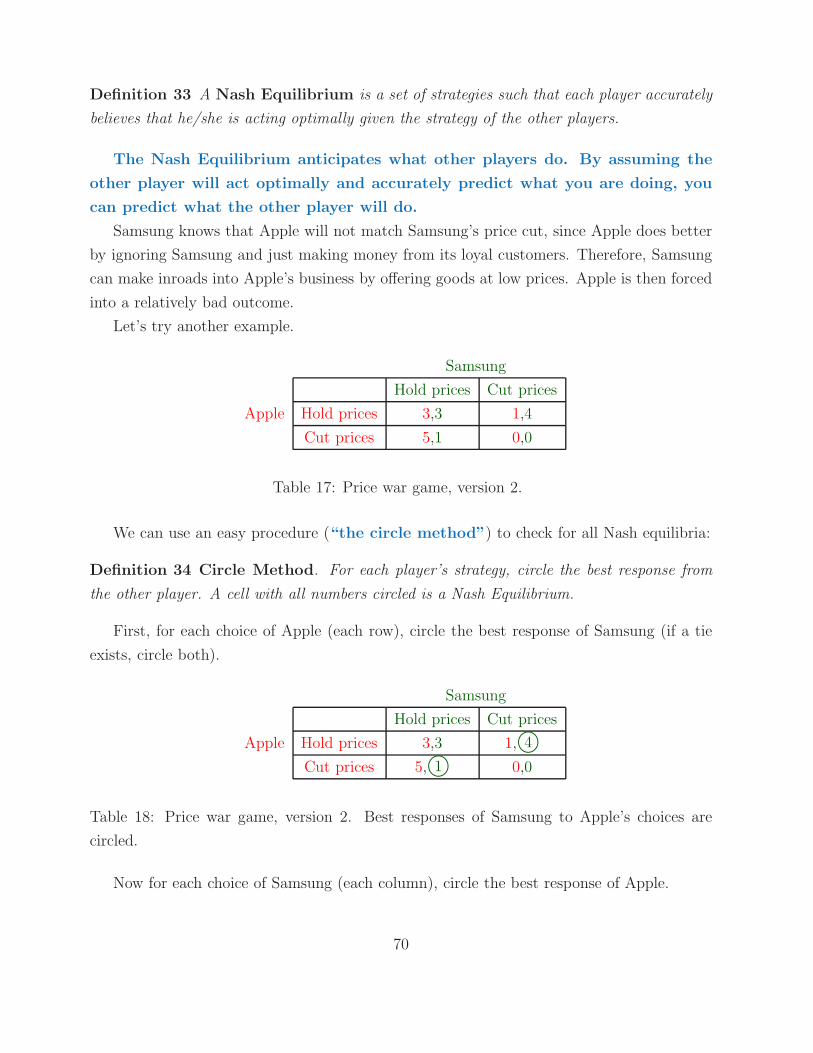
Definition 33 A Nash Equilibrium is a set of strategies such that each player accurately

believes that he/she is acting optimally given the strategy of the other players.

The Nash Equilibrium anticipates what other players do. By assuming the

other player will act optimally and accurately predict what you are doing, you

can predict what the other player will do.

Samsung knows that Apple will not match Samsung’s price cut, since Apple does better

by ignoring Samsung and just making money from its loyal customers. Therefore, Samsung

can make inroads into Apple’s business by offering goods at low prices. Apple is then forced

into a relatively bad outcome.

Let’s try another example.

Samsung


Apple Hold prices 3,3 1,4

Cut prices 5,1 0,0

Table 17: Price war game, version 2.

We can use an easy procedure (“the circle method”) to check for all Nash equilibria:

Definition 34 Circle Method. For each player’s strategy, circle the best response from

the other player. A cell with all numbers circled is a Nash Equilibrium.

First, for each choice of Apple (each row), circle the best response of Samsung (if a tie

exists, circle both).

Samsung


Apple Hold prices 3,3 1, 4©Cut prices 5, 1© 0,0

Table 18: Price war game, version 2. Best responses of Samsung to Apple’s choices are

circled.

Now for each choice of Samsung (each column), circle the best response of Apple.

70

Samsung


Apple Hold prices 3,3 1©, 4©Cut prices 5©, 1© 0,0

Table 19: Price war game, version 2. Best responses of both firms to each other’s choices

are circled.

The Nash equilibria are then the cells where both numbers are circled. In these cells,

each player’s action is a best response to the other players action. Here, two Nash equilibria

exist. The previous Nash equilibrium continues to hold:

• If Samsung predicts Apple holds,

• the Samsung does better by cutting,

• in which case Apple should hold. Since the prediction that A would hold is correct,

we have a Nash equilibrium. The Nash equilibrium is Apple holds and Samsung cuts.

But another Nash equilibrium exists:

• Suppose Samsung predicts Apple cuts.

• Then Samsung does at better by holding,

• in which case Apple should cut. Since the prediction is correct, we have a Nash

equilibrium.

Therefore the set of strategies “Apple cuts and Samsung holds” is also a Nash Equilibrium.

Often more than one Nash equilibrium exists, in which case the behavior gets harder to

predict.

Consider the “coordination” game of which side of the road to drive on.

Car B

B’s Left Side B’s Right Side

Car A A’s Left Side 10,10 -5,-5

A’s Right Side -5,-5 10,10

Table 20: Typical coordination game.

71

Circle the best responses to get the Nash equilibria:

Car B

B’s Left Side B’s Right Side

Car A A’s Left Side 10©, 10© -5,-5

A’s Right Side -5,-5 10©, 10©

Table 21: Typical coordination game.

If both drivers drive on the opposite sides of the road (from their own perspective), it

is a disaster for both players. But it does not matter if both players drive on their right or

left. Therefore, two Nash equilibria exist, and we should be able to observe that in some

countries people drive on the left and in other countries on the right.

II Some Simple Games

A Anti-Coordination Games: Avoiding Competition

“You should learn from your competitor, but never copy. Copy and you die.”

–Jack Ma (Alibaba founder)

Suppose firms need to decide which segment of the markets to target. Harley-Davidson

can build cruiser or sport motorcycles, and the same for Buell (another motorcycle man-

ufacturer). If both firms invest in the same business, competition will be fierce and each

company will price close to marginal cost, which is a problem especially given the fixed costs

of setting up the factory. However, if each focuses on a different market segment, both can

charge more and increase profits.

Buell

Sport Bikes Cruisers

Harley Sport Bikes 0,0 2,5

Cruisers 5,2 0,0

Table 22: Anti-coordination game.

Two Nash equilibria exist:

72

Buell

Sport Bikes Cruisers

Harley Sport Bikes 0,0 2©, 5©Cruisers 5©, 2© 0,0


In one Nash equilibrium, Harley specializing in cruisers and Buell sport bikes, and the

opposite in the second equilibrium. Notice that whoever gets the cruiser business is better

off since the cruiser business makes profits equal to 5. This can make the outcome somewhat

uneasy: both firms, deciding simultaneously, may choose cruisers and then hope the other

firm chooses sport bikes. Or if the game is not perfectly simultaneous, both firms may rush

into the cruiser business in the hopes that competitors will be deterred from doing so.

B Coordination Games

Firms sometimes play location coordination games. For example, firms that sell complemen-

tary goods, such as clothing and shoe stores, have incentives to locate together.

C Mixed Coordination and Anti-Coordination

Let’s try a tougher one of store location.

Target

Uptown Center City East Side West Side

Macy’s Uptown 30,40 50,95 55,95 55,120

Center City 115,40 100,100 130,85 120,95

East Side 125,45 95,65 60,40 115,120

West Side 105,50 75,75 95,95 35,55

Table 24: Location game. Coordinate or not?

The Nash equilibrium is found via:

73

Target

Uptown Center City East Side West Side

Macy’s Uptown 30,40 50,95 55,95 55,120©Center City 115,40 100©,100© 130©,85 120©,95

East Side 125©,45 95,65 60,40 115,120©West Side 105,50 75,75 95, 95© 35,55

Table 25: Location game. Coordinate or not?

In table 25, East Side and Center City are relatively affluent areas. Therefore, Macy’s

generally does better in these locations (all of the red circles are in rows 2 or 3). Target

does better in less affluent places (for example, two of Target’s circles are on the West

Side). However, if Target locates near Macy’s, then Target could draw more customers by

establishing the area as a place to shop (for example, when Macy’s locates at Center City,

target does best by also locating at Center City). Thus incentives exist to both coordinate

and anti-coordinate.

The Nash equilibrium is for both stores to locate at Center City (coordinate) and compete.

Restate the Nash equilibrium:

• Suppose Target forecasts that Macy’s locates at Center City.

• From the second row of table 24, the best response of Target is to locate at Center

City (100 beats all other payoffs).

• Check the forecast: if Target locates at Center City, Macy’s best response is to locate

at Center City (100 beats all alternatives in the second column). The forecast is correct

and so we have a Nash equilibrium.

Notice that the outcome could be better for both firms: Target could get $120 on the

West Side, but only if Macy’s locates Uptown or East Side. However, Macy’s will locate in

Center City if Target locates on the West Side. Macy’s does best by locating at Center City

and Target locates on the East Side. However, if Macy’s locates at Center City, Target will

follow.

Advantages of coordinating or not coordinating.

1. Coordinate by locating near competitors to draw shoppers to the area.

74

2. Coordinate by locating near competitors if demand in the area is better than

other areas (even with a competitor in the better area versus no competitor in the

worse area).

3. Coordinate if differentiating your product and being wrong about customer prefer-

ences yields more losses than the gains from sharing the market, but producing an

identical product.

4. Coordinate only if incumbent firms will not react forcefully to your entry.

D Prisoner’s Dilemmas

1 Example

Suppose a symmetric version of the price war game:

Firm B


Firm A Hold prices 3,3 0,5

Cut prices 5,0 1,1

Table 26: Prisoner’s dilemma game.

Firm B


Firm A Hold prices 3,3 0, 5©Cut prices 5©,0 1©, 1©

Table 27: Prisoner’s dilemma game.

So here a unique Nash Equilibrium exists where both firms cut prices (a price war ensues).

Notice a peculiar feature of this game: the outcome is relatively poor for both firms.

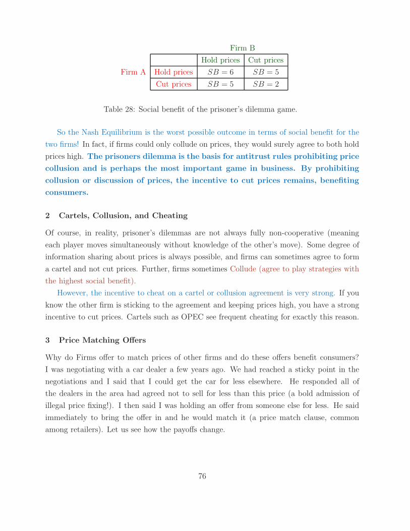
Definition 35 The Social Benefit is the sum of player payoffs, and the social benefit of the

game is the sum of player payoffs when both players play their Nash equilibrium strategies.

The social benefit is defined with respect to players only and not third parties like consumers.

So the upper left corner has a social benefit (SB) to the two firms (obviously not to the

consumers) of SB = 3 + 3 = 6. Similarly:

75

Firm B


Firm A Hold prices SB = 6 SB = 5

Cut prices SB = 5 SB = 2

Table 28: Social benefit of the prisoner’s dilemma game.

So the Nash Equilibrium is the worst possible outcome in terms of social benefit for the

two firms! In fact, if firms could only collude on prices, they would surely agree to both hold

prices high. The prisoners dilemma is the basis for antitrust rules prohibiting price

collusion and is perhaps the most important game in business. By prohibiting

collusion or discussion of prices, the incentive to cut prices remains, benefiting

consumers.

2 Cartels, Collusion, and Cheating

Of course, in reality, prisoner’s dilemmas are not always fully non-cooperative (meaning

each player moves simultaneously without knowledge of the other’s move). Some degree of

information sharing about prices is always possible, and firms can sometimes agree to form

a cartel and not cut prices. Further, firms sometimes Collude (agree to play strategies with

the highest social benefit).

However, the incentive to cheat on a cartel or collusion agreement is very strong. If you

know the other firm is sticking to the agreement and keeping prices high, you have a strong

incentive to cut prices. Cartels such as OPEC see frequent cheating for exactly this reason.

3 Price Matching Offers

Why do Firms offer to match prices of other firms and do these offers benefit consumers?

I was negotiating with a car dealer a few years ago. We had reached a sticky point in the

negotiations and I said that I could get the car for less elsewhere. He responded all of

the dealers in the area had agreed not to sell for less than this price (a bold admission of

illegal price fixing!). I then said I was holding an offer from someone else for less. He said

immediately to bring the offer in and he would match it (a price match clause, common

among retailers). Let us see how the payoffs change.

76

Firm B

Hold and match prices Cut prices

Firm A Hold and match prices 3,3 1,1

Cut prices 1,1 1,1

Table 29: Price matching game.

Now if one firm cuts prices, the other firm automatically matches and the gain from

cheating is erased. Two Nash Equilibria exist, one in which the cartel continues to hold and

the other which has both firms cutting prices.

Firm B

Hold and match prices Cut prices

Firm A Hold and match prices 3©, 3© 1©, 1

Cut prices 1, 1© 1©, 1©

Table 30: Price matching game.

However, the Nash equilibrium where both players hold and match is much more likely

to be observed, since hold and match is a dominant strategy for both firms.

If multiple Nash equilibria exist and players have a dominant strategy, then

we predict the dominant strategy equilibrium outcome.

So here both players have a dominant strategy to hold and match, so we predict both

players hold and match.

A price matching agreement does not suffer from cheating, like a cartel does. Thus price-

matching agreements are known to be instruments of price fixing, rather than benefiting

consumers.

E Example with 3 Players

A takeover specialist wishes to acquire a firm that has 3 major shareholders (Jack, April,

and Alec). The stock price is currently trading at $48. The specialist makes the following

offer: if one shareholder sells, she receives $65. If two shareholders sell, they each receive

$50. If all three sell, they each receive $45. The takeover succeeds if 2 or more shareholders

sell. If the takeover succeeds, then the specialist will dilute the shares so that the value of

77

any shares not sold is $40. If the takeover does not succeed, the payoff to those not selling

is $48, which is the original stock price. The payoffs are therefore:

Alec Sells

April

Sells Holds out

Jack Sells 45,45,45 50,40,50

Holds Out 40,50,50 48,48,65

Alec Holds Out

April

Sells Holds Out

Jack Sells 50,50,40 65,48,48

Holds Out 48,65,48 48,48,48

Table 31: Takeover game.

Pick any two player’s strategies, and circle the best response for the third player. For

example, if Alec picks Sell and Jack picks Sell, then comparing the two boxes comprising

the first row of the top table, we see that April should choose Sell because 45 > 40 (use the

second number in both boxes). If everyone else is selling, then the takeover will succeed, so

April must sell to prevent her shares from being diluted.

Analogously, suppose Jack and April both hold out. Comparing the bottom right corner

box in the top and bottom table, we see that Alec should sell since 65 > 48 (last number

in both boxes). In this case, Alec knows he is the only seller, and can therefore get the big

payoff from the takeover specialist.

For the rest:

78

Alec Sells

April

Sells Holds Out

Jack Sells 45©, 45©, 45© 50©,40, 50©Holds Out 40, 50©, 50© 48,48, 65©

Alec Holds Out

April

Sells Holds Out

Jack Sells 50©, 50©,40 65©,48,48

Holds Out 48, 65©,48 48,48,48

Table 32: Takeover game solution.

So the Nash equilibrium is that everyone sells and receives a price of $45, which is less

than the original value of the stock ($48)! The game is a prisoner’s dilemma in that everyone

would be better off everyone held out. But the specialist cleverly designed the payoffs to

give each shareholder a strong incentive to cheat on any agreement not to sell (if one or two

cheat, the payoffs are $65 and $50). Further, if two are selling, than the third must sell to

avoid dilution.3

III Mixed Strategies

When a player has an interest in disguising their actions, it is often optimal to choose a

random or mixed strategy.

Definition 36 A Mixed Strategy Nash Equilibrium is a Nash Equilibrium where the strategy

of at least one player assigns a random probability to choosing each strategy.

Definition 37 A Pure Strategy Nash Equilibrium is a Nash Equilibrium where the strategy

of each player is chosen with probability one.

We have previously only considered pure strategies, but will now look at mixed strategies.

3This example combines some actual cases. Decreasing the sale price if more shareholders sell has been

used in the takeover of Federated Department Stores in 1998. Dilution or otherwise penalizing hold outs is a

common strategy. See for example, the Facebook movie, or the treatment of hold out creditors by Argentina.

79

A Using Mixed Strategies to Prevent Opponents From Reacting

Sellers sometimes offer sales at random times. The classic example is the “Blue Light Special”

where at random times a sale is announced over the retailer’s PA system. The seller wants

to get rid of excess inventory. But if the seller announces a sale on a specific date, then all

customers would shop on that date only, including those who would have bought the product

at the high price. What would be ideal is if non price sensitive customers did not change

their behavior in response to when the sale was.

Customer

Shop today Shop tomorrow

Firm Sale today 4,12 8,6

Sale Tomorrow 12,8 6,10

Table 33: Blue light special game.

The customer (lets say this customer would buy at full price) is better off shopping on

the day when the sale is. The firm is better off if this customer comes on a day when there

is no sale. The firm wants to anti-coordinate and the shopper wants to coordinate.

No Pure Strategy Nash Equilibrium exists in this game. Suppose the firm predicts

customers will shop today. Then the firm chooses to have the sale tomorrow. But then after

announcing the sale, customers will shop tomorrow, so customers shopping today is not a

Nash Equilibrium. Similarly, if the firm predicts shoppers will shop tomorrow and announces

a sale for today, then customers react by shopping today and the firm regrets the decision

to have a sale today.

But an equilibrium exists in which consumers and firms assign probabilities to strategies

(the Blue Light Special). Suppose the firm offers a sale today with probability q. Then the

customer who shops today gets 12 with probability q and 8 with probability 1− q for a total

of 12q + 8 (1− q). The payoff for shopping tomorrow is 6q + 10 (1− q). The seller must

equalize the two average payoffs. If the average payoffs are different, the shopper will

always shop on one day, but then the firm will want to have the sale on the other day, and

the prediction that the seller randomizes is not correct. So the equilibrium breaks down if

the the average payoffs are not equal.

So we have:

12q + 8 (1− q) = 6q + 10 (1− q) (170)

80

4q = 1 → q =1

4(171)

So having a sale one quarter of the time today, and 3/4 of the time tomorrow is the best

the firm can do. Notice that consumer overall prefers to shop today (adding the columns,

12 + 8 > 6 + 10). Therefore, the seller must have a higher probability of a sale tomorrow.

If the probabilities of a sale were equal on the two days, the shopper would definitely shop

today and the equilibrium would break down. Only by making a sale less likely today can

the seller make the buyer indifferent.

Similarly, the consumer does not want to give away to the firm which day they will be

shopping, so they also randomize. Let p be the probability that a consumer shops today.

The payoff to the firm of a sale today is then 4p+8 (1− p) and the payoff of a sale tomorrow

is 12p+ 6 (1− p). Equalizing these two gives:

4p+ 8 (1− p) = 12p+ 6 (1− p) (172)

1− p = 4p → p =1

5(173)

So the shopper sets p to equalize the average payoffs to the seller. If the payoffs to seller

are not equal, the seller always holds the sale on one day, but then the shopper does not

randomize, and the equilibrium breaks down. So the mixed strategy Nash Equilibrium is to

shop today with probability 1/5 and to have a sale today with probability 1/4.

In mixed strategies, each player deters other players from playing their favorite strategy.

Without this deterrence players would play their favorite strategy all the time, but then

we would be back to using pure strategies with no equilibrium. We can find each player’s

favorite strategy by supposing the other player chooses a probability of 1/2. Since the

strategies are weighted equally, the opposing player might as well just play their favorite

strategy. If the firm chooses sale today with probability 1/2, the customer’s payoffs are

0.5 (12 + 8) > 0.5 (6 + 10). Hence the customer’s favorite strategy is to shop today. The

firm has a sale more often tomorrow to deter the customer from shopping today all the time.

It is important to understand what the Nash Equilibrium is:

• The shopper predicts the firm will have a sale today with probability 1/4. The shop-

per does not predict an outcome. The shopper only predicts a strategy (a probability).

• The firm predicts the shopper will shop today with probability 1/5. The firm also does

not know the outcome, but only predicts a probability.

81

• Given the predictions, the shopper does at least as well shopping today with probability

1/5 as shopping today with any other probability. So the shopper plays this strategy

and the prediction (of a probability, not an outcome) is correct. The same reasoning

holds for the firm.

Other examples of games of this type include Rock, paper, scissors; baseball (fastball or

curve); penalty kicks (left or right side); and tennis (serve inside or outside). Studies have

found that humans are not great randomizers. Two common pitfalls:

1. Players switch too often. For example, studies of tennis players show they switch

too often between serving inside and outside. A smart opponent can therefore gain an

advantage by guessing the serve will go to the opposite side as the previous serve.

2. Players try too hard to ensure all possible strategies occur. In the TV show

“Numbers” a serial killer appears to be killing in random neighborhoods. However, the

police are able to catch the killer by predicting he will strike in a previously untouched

neighborhood, rather than striking a second time in another neighborhood.

B Using Mixed Strategies to Avoid Coordination

Consider two firms, Macy’s and TJ Maxx. Macy’s is a high priced retailer that carries

a variety of clothes in all sizes (and thus higher inventory costs and higher prices) and TJ

Maxx is a retailer who charges low prices, but carries whatever surplus clothes manufacturers

happen to have, usually in odd sizes. Customers can shop at Macy’s, putting up with high

prices but knowing they will find what they want, or they can go to TJ Maxx, paying lower

prices if TJ Maxx happens to have what they want. Further, the more customers go to TJ

Maxx, the more likely they are to be out of something. So the payoffs are:

Jack

Shop TJ Maxx Shop Macy’s

April Shop TJ Maxx 4,4 10,7

Shop Macy’s 7,10 5,5


Here two Nash Equilibria exist, corresponding to the customers shopping at different

stores.

82

• If Jack predicts April will shop at Macy’s, then Jack knows TJ Maxx likely has Jack’s

size and will have lower prices. But then April will shop at Macy’s and we have a Nash

equilibrium.

• The game is symmetric (Jack and April are identical in terms of payoffs), so April

shops at TJ Maxx and Jack shops at Macy’s is also an equilibrium.

Now compute a mixed strategy.

• Suppose Jack predicts April will shop at TJ Maxx with probability q.

• Then Jack’s payoff is 4q + 10 (1− q) if Jack shops at TJ Maxx and 7q + 5 (1− q) if

Jack shops at Macy’s. Payoffs are equal if q = 5

8.

• The game is symmetric, so a mixed strategy exists in which each customer shops at

the discount retailer with probability 5/8.

Notice that the mixed strategy is not very efficient. With probability 5

8· 58= 25

64the customers

“bump into each other” at the discount store, which does not lead to a high payoff for either

player. The social benefit of either pure strategy Nash equilibria is 7 + 10 = 17. The social

benefit of the mixed strategy is the sum of the social benefits times the probability of end

up in each box:

5

8·5

8· (4 + 4) +

5

8·3

8· (10 + 7) +

3

8·5

8· (7 + 10) +

3

8·3

8· (5 + 5) = 13.5, (174)

which is less than the social benefit of the pure strategy Nash. Nonetheless, the mixed Nash

may be more realistic, because both players prefer the discount store, so both players have

an incentive to pick TJ Maxx.

By the way, this game was featured in the movie about John Nash: “A Beautiful Mind.”

However, the movie inexplicably states that the Nash Equilibrium is for all consumers to

shop at the high priced retailer. Nash proved in his dissertation that every game has at least

one mixed or pure strategy equilibrium.

IV Dynamic Sequential Games

Two versions of games played over time exist: games as above but repeated, and sequential

games in which one player moves before the other. We will look at only the sequential games.

83

A Extensive Form

It is easiest to represent sequential games in extensive form. In the extensive form, player

strategies are represented as branches on a tree.

Consider an anti-coordination game where one player now moves first. Apple, the first

mover, can either expand capacity in the tablet market or not expand capacity. Then

Samsung has the same choice. As in the anti-coordination game, if both firms expand in the

tablet market, the competition will be fierce and profits are low for both firms. If one firm

expands and the other firm does not, profits will be high for the firm that expands. The

firm that does not enter makes more money than the case where both firms expand into the

tablet market, but less than if the firm entered and the other firm did not.

Samsung

Don’t Expand

Expand

Expand

Don’t Expand

Expand

Don’t Expand

Apple: $50 Million

Samsung: $50 Million

Apple: $150 Million


Apple: $60 Million


Apple: $80 Million


Samsung

Apple

Figure 10: Anti-coordination game in sequential form.

To solve this problem, work backwards. If Apple expands, Samsung does better by ceding

Apple the market and focusing resources elsewhere. If Apple does not expand, Samsung

does better by expanding into the tablet business. Knowing this, Apple can either expand,

knowing Samsung will not expand, and make $150 Million, or not expand, knowing Samsung

84

will expand, and make $60 million. Thus Apple will expand. The equilibrium, which we will

call Sub-Game Perfect, is for Apple to Expand and Samsung not to Expand. Apple makes

$150 Million and Samsung makes $60 Million.

Apple earns$60 here

Apple earns$150 here


Apple

Samsung

Samsung

Sub−game perfect

Don’t Expand

Expand

Expand

Don’t Expand

Expand

Don’t Expand

Apple: $50 Million


Apple: $150 Million


Apple: $60 Million


Apple: $80 Million

Equilibrium

Path

Nash eq.


Definition 38 A Sub-Game Perfect Equilibrium requires each sub-tree to be a Nash

Equilibrium.

Sub-game perfect requires beliefs to be correct, even off the equilibrium path. The

equilibrium path is the sequence of decisions players actually make during the game. In

Figure (11), Apple Expands, and then Samsung does not is on the equilibrium path. The

situation where Apple does not expand and Samsung does expand never occurs and is thus off

the equilibrium path. Sub-game perfect requires beliefs to be correct even off the equilibrium

path: Apple must correctly believe Samsung will expand if Apple doesn’t, even though we

never actually see this part of the game.

Consider an alternative equilibrium definition:

Definition 39 A Nash Equilibrium (not sub-game perfect) requires only that beliefs

85

are correct along the equilibrium path. That is, only the sub-games actually observed must

be Nash equilibria.

In the above example, a Nash equilibrium which is not sub-game perfect exists. Suppose

Samsung threatens to expand if Apple expands. If Apple believes this threat, then Apple

does best by not expanding. If Apple does not expand, then Apple’s belief that Samsung will

expand if Apple expands is never put to the test. So the equilibrium satisfies the definition

of a Nash equilibrium since all beliefs are correct along the equilibrium path.


Expand

Expand

Don’t Expand

Expand

Don’t Expand

Apple: $50 Million


Apple: $150 Million


Apple: $60 Million


Apple: $80 Million

Apple

Samsung

Samsung

Sub−game perfect

Apple earns$60 here

Don’t Expand

Apple earns $50

Beliefs must be correct

along equilibrium path only

Nash (not subgame

perfect)

Non-credible

If Apple believes

here

Nash eq.

Threat

Equilibrium

path


However, the Nash equilibrium which is not sub-game perfect is less realistic in that the

threat is not credible (Apple should call Samsung’s bluff here).

In the simultaneous game, two Nash Equilibria exist and both players prefer a different

equilibria.

86

Samsung

Expand Don’t Expand

Apple Expand 50,50 150,60

Don’t Expand 60,120 80,80

Table 35: Simultaneous first mover game.

Apple prefers the Nash equilibrium in the upper right corner of table 35, whereas Samsung

prefers the Nash equilibrium in the lower left corner. The first mover gets an advantage which

results in the selection of the first mover’s preferred Nash Equilibrium. That is, the preferred

Nash equilibrium of the first mover in the simultaneous game is sub-game perfect.

Definition 40 First Mover Advantage: Advantage to the first mover in sequential games

when the simultaneous game has multiple Nash Equilibria.

We see in this example that sub-game perfect equilibria are more stringent than Nash

Equilibria (only 1 equilibrium exists, not two).

B Preemption and Deterrence

“Success breeds complacency. Complacency breeds failure. Only the paranoid

survive.” –Andy Groves

An important strategy for the market leader in an industry is to deter entry by potential

rivals. Suppose Intel dominates in terms of market share the market for computer memory

chips. Intel knows a number of other makers of electronic parts could enter the market at

any time, for example AMD. The payoff matrix is:

87

Don’t Cut Prices

Intel

Intel

Don’t Cut Prices

Cut Prices

Cut Prices

Enter

Don’t Enter

AMD

AMD: $6 Million

Intel: $3 Million

AMD: $12 Million

Intel: $4 Million

AMD: $9 Million

AMD: $9 Million

Intel: $13 Million

Intel: $8 Million

Figure 13: Entry game.

AMD moves first, by deciding whether or not to enter. Then Intel decides whether to

respond by cutting prices and expanding output, or ignoring AMD and sharing the market.

We solve the problem by working backward. First, if AMD enters, then an ensuing price war

would mean that Intel’s profits are lower than if it instead kept prices high, making money

from the most loyal customers, while ceding some of the market to AMD. If AMD does not

enter, than Intel of course does much better holding prices high. So AMD has the choice of

entering, knowing that Intel will not cut prices or not entering. Thus AMD enters.

88

AMD $9

Intel

Intel

Don’t Cut Prices

Cut Prices

Cut Prices

Enter

Don’t Enter

AMD

AMD: $6 Million

Intel: $3 Million

AMD: $12 Million

Intel: $4 Million

AMD: $9 Million

AMD: $9 Million

Intel: $13 Million

Intel: $8 Million

Don’t Cut Prices

AMD; $12


Intel can threaten to cut prices, but AMD knows the threat is not credible and enters.

Sub-game perfection requires threats to be credible while the Nash Equilibrium does not. To

see this, suppose AMD predicts Intel will cut prices if AMD enters. Then AMD should not

enter. Then Nash Equilibria requires us to check whether or not our prediction is correct.

But in this case the prediction does not matter, because AMD has decided not to enter. So

we can say the prediction is correct.

Next suppose we add another move for Intel. Intel can add capacity or not add capacity

before AMD decides whether or not to enter. If Intel adds capacity, then Intel can efficiently

produce a large volume of chips if AMD enters. However, the expansion results in $2 million

of extra fixed costs if the factory is not used. The payoff matrix then changes as shown

below, and AMD decides not to enter. Building capacity is one way to make threats more

credible and deter entry. Building excess capacity is of course costly, however.

89

Intel: $11 Million

Intel: $3 Million

AMD: $6 Million

Intel: $3 Million

AMD: $12 Million

Intel: $4 Million

AMD: $9 Million

Intel: $8 Million

AMD: $9 Million

Intel: $13 Million

Enter

Don’t Enter

Intel

Intel

Cut Prices

Don’t Cut Prices

Cut Prices

Don’t Cut Prices

Enter

Don’t Enter

Intel

Intel

Cut Prices

Don’t Cut Prices

Cut Prices

Don’t Cut Prices

AMD

AMD

Intel

Don’t Expand

ExpandAMD: $12 Million

Intel: $2 Million

AMD: $9 Million

Intel: $6 Million

AMD: $9 Million

AMD: $6 Million


90

AMD $9

Intel: $3 Million

AMD: $6 Million

Intel: $3 Million

AMD: $12 Million

Intel: $4 Million

AMD: $9 Million

Intel: $8 Million

AMD: $9 Million

Intel: $13 Million

Enter

Don’t Enter

Intel

Intel

Cut Prices

Don’t Cut Prices

Cut Prices

Don’t Cut Prices

Enter

Don’t Enter

Intel

Intel

Cut Prices

Don’t Cut Prices

Cut Prices

Don’t Cut Prices

AMD

AMD

Intel

Don’t Expand

ExpandAMD: $12 Million

Intel: $2 Million

AMD: $9 Million

Intel: $6 Million

AMD: $9 Million

Intel: $11 Million

Intel $4

Intel $11

AMD: $12

AMD: $9

AMD $6

AMD: $6 Million

Figure 16: Entry game with capacity decision.

The excess capacity means it is more profitable for Intel to cut prices if AMD enters.

Therefore, the expansion by Intel deters entry by AMD. Intel takes a preemptive action, to

deter AMD from entering. Examples of entry deterrence:

1. DuPont in 1979 invests $0.33 billion in titanium dioxide plants to deter rivals with

older plants from updating to newer, more competitive plants.

2. Walmart’s strategy is to build large stores in smaller towns first in order to deter others

from building similar stores, since each town can support at most one store.

Definition 41 Preemption is an action taken to deter later actions by other players.

91

• Preemption allows the firm to gain a first mover advantage.

• The preemptive action must be permanent (irreversible) action. It is not a threat.

• Rule from game theory: it is better to anticipate and preempt than to react.

It is easy for a market leader to become complacent and not take action until after a

rival has entered. This is often too late.

V Summary: Lessons from Eco 685!

To summarize, I would like to leave you with a few takeaway lessons from the class.

1. Incentives matter. When structuring pay, you get what you measure and reward.

2. Be on the lookout for better opportunities. Avoid committing time and resources

to low-profit endeavors.

3. Think marginally. Think: is this hire going to bring in more revenue that his/her

salary? Think: is this client going to bring in more revenue than the cost of servicing

the client? Avoid thinking in terms of averages. These tell you only what has happened

in the past.

4. Ignore sunk costs. It is sometimes painful, but one has to sometimes ignore the

sunk costs and move on. Hanging on too long because of past investments can cause

more pain later.

5. Work hard to get to the right scale. Many firms (especially small firms) can lower

costs by scaling up. Find a way (merge/expand) to get to an ideal size. Conversely,

for large firms think about if your scale is too large.

6. Embrace competition. Everyone has competitors. Profitable businesses can expect

new competitors will arrive soon. Realize competition exists and use it to improve

your product/business.

7. Use advanced pricing tricks. Profits are not easy to come by. Getting some extra

profits by charging different prices to different groups (price discrimination and/or

upcharging) is one of the few easy ways to increase profits.

8. Predict: how will competitors react to my plan? Try to anticipate the reaction

of other firms and coworkers to your plans.

92

9. Remember: other firms and consumers will eventually react to your deci-

sions. Avoid decisions which are easy to react to, such as having a sale at the end of

every month. Consumers will catch on quickly.

10. Segment markets. Avoid head-to-head competition. In general, it is better to

segment a market by producing a version of a product which is of interest only to a

subset of the consumers, than to compete head on with an established firm.

11. Preempt, do not react. Acting preemptively is always cheaper and more decisive

than reacting to moves by other firms.

93

STRATEGY - Miami

Documents

Transcript of STRATEGY - Miami